deformed (nilsson) shell model - gsiwolle/telekolleg/kern/... · deformed (nilsson) shell model...
TRANSCRIPT
Deformed (Nilsson) shell model
Introduction to Nuclear Science
Simon Fraser UniversitySpring 2011
NUCS 342 — January 31, 2011
NUCS 342 (Lecture 9) January 31, 2011 1 / 35

Outline
1 Infinitely deep potential well in three dimensions
1 Spherical infinitely deep potential well in three dimensions
2 Axial infinitely deep potential well in three dimensions
3 The Nilsson model
NUCS 342 (Lecture 9) January 31, 2011 2 / 35
Outline
1 Infinitely deep potential well in three dimensions
1 Spherical infinitely deep potential well in three dimensions
2 Axial infinitely deep potential well in three dimensions
3 The Nilsson model
NUCS 342 (Lecture 9) January 31, 2011 2 / 35
Outline
1 Infinitely deep potential well in three dimensions
1 Spherical infinitely deep potential well in three dimensions
2 Axial infinitely deep potential well in three dimensions
3 The Nilsson model
NUCS 342 (Lecture 9) January 31, 2011 2 / 35
Outline
1 Infinitely deep potential well in three dimensions
1 Spherical infinitely deep potential well in three dimensions
2 Axial infinitely deep potential well in three dimensions
3 The Nilsson model
NUCS 342 (Lecture 9) January 31, 2011 2 / 35
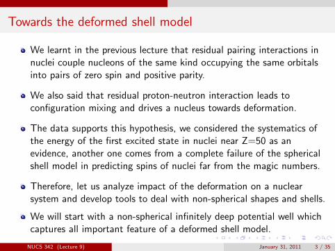
Towards the deformed shell model
We learnt in the previous lecture that residual pairing interactions innuclei couple nucleons of the same kind occupying the same orbitalsinto pairs of zero spin and positive parity.
We also said that residual proton-neutron interaction leads toconfiguration mixing and drives a nucleus towards deformation.
The data supports this hypothesis, we considered the systematics ofthe energy of the first excited state in nuclei near Z=50 as anevidence, another one comes from a complete failure of the sphericalshell model in predicting spins of nuclei far from the magic numbers.
Therefore, let us analyze impact of the deformation on a nuclearsystem and develop tools to deal with non-spherical shapes and shells.
We will start with a non-spherical infinitely deep potential well whichcaptures all important feature of a deformed shell model.
NUCS 342 (Lecture 9) January 31, 2011 3 / 35

Infinitely deep potential well in one dimension
If the well is infinitely deep the Schrodinger equation requires that thewave function vanishes on the boundaries.
NUCS 342 (Lecture 9) January 31, 2011 4 / 35

Infinitely deep potential well in one dimension
For the well on the graph
ψ(0) = 0 ψ(L) = 0 =⇒ ψ(x) = A sin(nπ
Lx)
But at the same time
ψ(x) = A sin(kx) ~k =√
2mE
This leads to
k =1
~√
2mE =nπ
Lor
E = n2 π2~2
2mL2= n2E1 E1 =
h2
8mL2
Note that the wave function for the ground state is symmetric withrespect to the middle of the well (has positive parity), for the nextstate the wave function is asymmetric (has negative parity) etc.
NUCS 342 (Lecture 9) January 31, 2011 5 / 35
Infinitely deep potential well in three dimensions
In a Cartesian space the coordinates x , y and z are independent ofeach other.
Therefore we can think about a three-dimensional infinitely deeppotential well as about three independent wells constraining particlemotion along each of the independent coordinate.
A consequence of that fact is separation of variables in theSchrodinger equation, the three-dimensional equation can be splitinto three one-dimensional equations.
The wave function is a product of three one-dimensional wavefunction, each being a solution for the one-dimensional equation foreach of the coordinates.
The energy is the sum of three energies corresponding to the solutionfor the one-dimensional equation for each of the coordinates.
NUCS 342 (Lecture 9) January 31, 2011 6 / 35

Separation of variables
For the potential
V (x , y , z) = V (x) + V (y) + V (z) (1)
For the wave function
Ψ(x , y , z) = Ψ(x)Ψ(y)Ψ(z) (2)
For the equation
EΨ(x , y , x) =
− ~2
2m
(∂2
∂x2+
∂2
∂y2+
∂2
∂z2
)+ V (x , y , z)
Ψ(x , y , z) =
= Ψ(y)Ψ(z)
(− ~2
2m
d2
dx2+ V (x)
)Ψ(x) +
Ψ(x)Ψ(z)
(− ~2
2m
d2
dy2+ V (y)
)Ψ(y) +
Ψ(x)Ψ(y)
(− ~2
2m
d2
dz2+ V (z)
)Ψ(z) (3)
NUCS 342 (Lecture 9) January 31, 2011 7 / 35
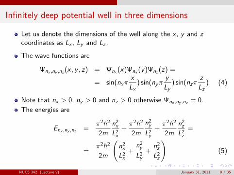
Infinitely deep potential well in three dimensions
Let us denote the dimensions of the well along the x , y and zcoordinates as Lx , Ly and Lz .
The wave functions are
Ψnx ,ny ,nz (x , y , z) = Ψnx (x)Ψny (y)Ψnz (z) =
= sin(nxπx
Lx) sin(nyπ
y
Ly) sin(nzπ
z
Lz) (4)
Note that nx > 0, ny > 0 and nz > 0 otherwise Ψnx ,ny ,nz = 0.
The energies are
Enx ,ny ,nz =π2~2
2m
n2x
L2x
+π2~2
2m
n2y
L2y
+π2~2
2m
n2z
L2z
=
=π2~2
2m
(n2x
L2x
+n2y
L2y
+n2z
L2z
)(5)
NUCS 342 (Lecture 9) January 31, 2011 8 / 35
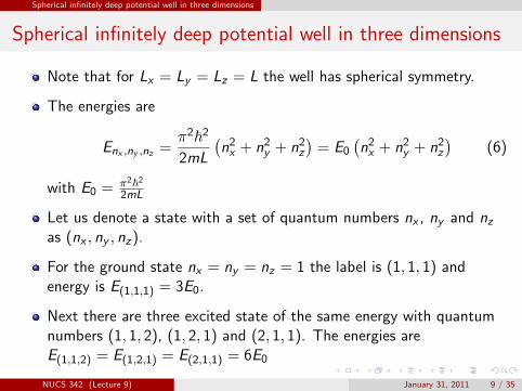
Spherical infinitely deep potential well in three dimensions
Spherical infinitely deep potential well in three dimensions
Note that for Lx = Ly = Lz = L the well has spherical symmetry.
The energies are
Enx ,ny ,nz =π2~2
2mL
(n2x + n2
y + n2z
)= E0
(n2x + n2
y + n2z
)(6)
with E0 = π2~2
2mL
Let us denote a state with a set of quantum numbers nx , ny and nzas (nx , ny , nz).
For the ground state nx = ny = nz = 1 the label is (1, 1, 1) andenergy is E(1,1,1) = 3E0.
Next there are three excited state of the same energy with quantumnumbers (1, 1, 2), (1, 2, 1) and (2, 1, 1). The energies areE(1,1,2) = E(1,2,1) = E(2,1,1) = 6E0
NUCS 342 (Lecture 9) January 31, 2011 9 / 35

Spherical infinitely deep potential well in three dimensions
Degenerate states
Let us have a closer look at the three states at energy E = 6E0.
The quantum numbers (1, 1, 2), (1, 2, 1) and (2, 1, 1) indicate thatthey have a different quantum numbers, thus, they have differentwave functions.
Different wave functions indicate different states. But forLx = Ly = Lz = L the energy E = E0(n2
x + n2y + n2
z) is the same forall three states. States of different wave function but the same energyare called degenerate states.
The level of degeneracy is the number of states at a given energy. Forstates at the energy E = 6E0 the level of degeneracy is three.
Note that the next level is also degenerate with the level ofdegeneracy of three, quantum numbers (2, 2, 1), (2, 1, 2) and (1, 2, 2)and energy E = 9E0.
NUCS 342 (Lecture 9) January 31, 2011 10 / 35

Spherical infinitely deep potential well in three dimensions
Spherical infinitely deep potential well in three dimensions
Here are the parameters of low-energy states in spherical infinitelydeep potential well in three dimensions
Energy Degeneracy Quantum numbers
3E0 1 (1, 1, 1)6E0 3 (1, 1, 2), (1, 2, 1), (2, 1, 1)9E0 3 (2, 2, 1), (2, 1, 2), (1, 2, 2)
11E0 3 (1, 1, 3), (1, 3, 1), (3, 1, 1)12E0 1 (2, 2, 2)
In this model the energies are the energies of the major shells, thedegeneracy defines the number of particles or occupancy of the shell.
The most important consequence of the deformation is a change inenergy and the level of degeneracy of shells.
The deformation destroys spherical shell gaps and open new gaps anddifferent magic numbers.
NUCS 342 (Lecture 9) January 31, 2011 11 / 35

Axial infinitely deep potential well in three dimensions
Deformed shapes
The simplest deviation from spherical symmetry is for one dimensionof the well to be different of the other two, with the other two beingequal.
This corresponds to axially symmetric potential well with thenon-equal dimension being along the symmetry axis, and the othertwo dimension being perpendicular to the symmetry axis.
Traditionally, the symmetry axis is taken as the z axis of thecoordinate frame Lz 6= Lx = Ly .
We can distinguish two cases of axial deformation, prolateLz > Lx = Ly and oblate Lz < Lx = Ly .
These are the cases we are going to analyze. There is also the triaxialcase Lz 6= Ly 6= Lx which is absolutely legitimate, but we have notime to analyze it.
NUCS 342 (Lecture 9) January 31, 2011 12 / 35
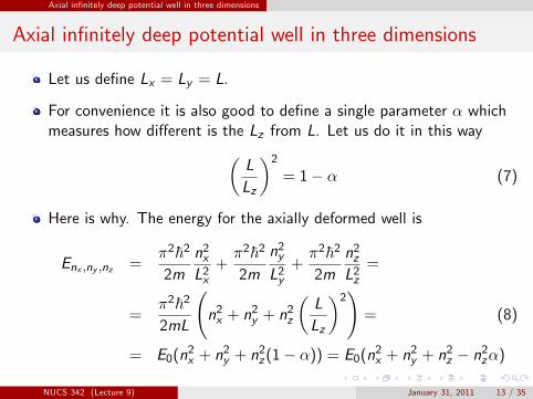
Axial infinitely deep potential well in three dimensions
Axial infinitely deep potential well in three dimensions
Let us define Lx = Ly = L.
For convenience it is also good to define a single parameter α whichmeasures how different is the Lz from L. Let us do it in this way(
L
Lz
)2
= 1− α (7)
Here is why. The energy for the axially deformed well is
Enx ,ny ,nz =π2~2
2m
n2x
L2x
+π2~2
2m
n2y
L2y
+π2~2
2m
n2z
L2z
=
=π2~2
2mL
(n2x + n2
y + n2z
(L
Lz
)2)
= (8)
= E0(n2x + n2
y + n2z(1− α)) = E0(n2
x + n2y + n2
z − n2zα)
NUCS 342 (Lecture 9) January 31, 2011 13 / 35
Axial infinitely deep potential well in three dimensions
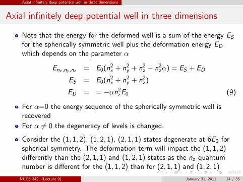
Axial infinitely deep potential well in three dimensions
Note that the energy for the deformed well is a sum of the energy ES
for the spherically symmetric well plus the deformation energy ED
which depends on the parameter α
Enx ,ny ,nz = E0(n2x + n2
y + n2z − n2
zα) = ES + ED
ES = E0(n2x + n2
y + n2z)
ED = = −αn2zE0 (9)
For α=0 the energy sequence of the spherically symmetric well isrecovered
For α 6= 0 the degeneracy of levels is changed.
Consider the (1, 1, 2), (1, 2, 1), (2, 1, 1) states degenerate at 6E0 forspherical symmetry. The deformation term will impact the (1, 1, 2)differently than the (2, 1, 1) and (1, 2, 1) states as the nz quantumnumber is different for the (1, 1, 2) than for (2, 1, 1) and (1, 2, 1)
NUCS 342 (Lecture 9) January 31, 2011 14 / 35

Axial infinitely deep potential well in three dimensions
Axial infinitely deep potential well in three dimensions
0
2
4
6
8
10
12
14
16
-0.6 -0.4 -0.2 0 0.2 0.4 0.6
E/E
0
α
(1,1,1)
(2,1,1)
(1,2,1)
(2,2,1)(1,3,1)
(3,1,1)
(1,1,2)
(1,2,2)(2,1,2)
(2,2,2) (1,1,3)
NUCS 342 (Lecture 9) January 31, 2011 15 / 35

Axial infinitely deep potential well in three dimensions
Why does the energy change?
Recall that the energy is directly proportional to the frequency of thewave function or inversely proportional to the wave length.
The wave function has nodes at the boundaries of the well, thus thewave length is define by the size of the well.
If the well gets larger the wave length of the wave function increases,the frequency decreases and energy is reduced.
In a contrary, if the well size decreases the wave length decreases, thefrequency increases and the energy increases.
Recall that
Lz = L1√
1− α≈ L(1 +
1
2α) (10)
thus for positive α the well becomes prolate, the Lz increases andenergy decreases, while for the negative α Lz decreases and energyincreases.
NUCS 342 (Lecture 9) January 31, 2011 16 / 35

Axial infinitely deep potential well in three dimensions
Why atoms do not deform?
If deformation reduces energy of a system why atoms do not deform?Indeed, all atoms are found to be spherical, but the deformed shellmodel features we investigated are generic. Should they be applicableto atoms as well?
The answer is in the central role and tiny size of a nucleus.
Since the force bounding atom comes from the nucleus and this forcedominates any other forces, if this force has spherical symmetry thewhole atom does.
Object of any shape when looked from afar looks point-like. A pointhas the same symmetry as a sphere.
This is the case for nucleus in atoms. Even if deformed it is separatedby electrons by a large distance, so the impact of the nucleardeformation on the shape of an atom is minimal. However, there is animpact on the structure of the atomic levels (hyperfine structure).
NUCS 342 (Lecture 9) January 31, 2011 17 / 35

Axial infinitely deep potential well in three dimensions
Why atoms do not deform?
The size of the atom is ∼0.1 [nm] the size of a nucleus∼1 [fm]=10−4 [nm]. Thus electrons are separated from a nucleus bya distance which is ∼10000 times larger than the nucleus.
Nuclear deformation is not larger than the size of a nucleus.
On average for an electron to see a nucleus deformed it is similar for ahuman being to see a deformation of a soccer ball (1 foot indiameter) from a plane being 10000 feet above the ground.
Good luck.
NUCS 342 (Lecture 9) January 31, 2011 18 / 35
Axial infinitely deep potential well in three dimensions
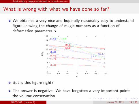
What is wrong with what we have done so far?
We obtained a very nice and hopefully reasonably easy to understandfigure showing the change of magic numbers as a function ofdeformation parameter α.
0
2
4
6
8
10
12
14
16
-0.6 -0.4 -0.2 0 0.2 0.4 0.6
E/E
0
α
(1,1,1)
(2,1,1)
(1,2,1)
(2,2,1)(1,3,1)
(3,1,1)
(1,1,2)
(1,2,2)(2,1,2)
(2,2,2) (1,1,3)
But is this figure right?
The answer is negative. We have forgotten a very important point:the volume conservation.
NUCS 342 (Lecture 9) January 31, 2011 19 / 35
Axial infinitely deep potential well in three dimensions
Volume conservation
In previous lectures we discussed incompressibility of nuclear matter.
This implies that nuclear deformation has to conserve volume.
The deformation we considered so far made one of the dimensions ofthe well longer or shorter while keeping the other two together.
This deformation does not conserve the volume.
To conserve the volume when axially deforming the well we need tomake the dimensions perpendicular to the symmetry axis shorter whenthe dimension along the axis gets longer, or the other way around.
This implies that all three axes need to change the length whiledeformation occurs.
Change of the axes length has a direct impact on state energies.
NUCS 342 (Lecture 9) January 31, 2011 20 / 35
Axial infinitely deep potential well in three dimensions
Volume conservation
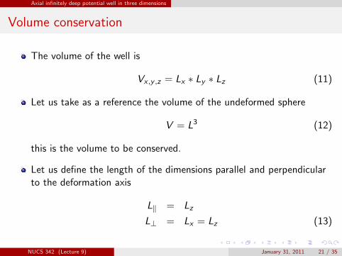
The volume of the well is
Vx ,y ,z = Lx ∗ Ly ∗ Lz (11)
Let us take as a reference the volume of the undeformed sphere
V = L3 (12)
this is the volume to be conserved.
Let us define the length of the dimensions parallel and perpendicularto the deformation axis
L‖ = Lz
L⊥ = Lx = Lz (13)
NUCS 342 (Lecture 9) January 31, 2011 21 / 35
Axial infinitely deep potential well in three dimensions
Volume conservation
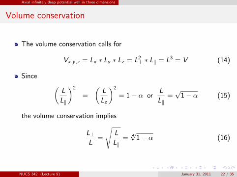
The volume conservation calls for
Vx ,y ,z = Lx ∗ Ly ∗ Lz = L2⊥ ∗ L‖ = L3 = V (14)
Since (L
L‖
)2
=
(L
Lz
)2
= 1− α orL
L‖=√
1− α (15)
the volume conservation implies
L⊥L
=
√L
L‖= 4√
1− α (16)
NUCS 342 (Lecture 9) January 31, 2011 22 / 35

Axial infinitely deep potential well in three dimensions
Volume conservation
The energies including volume conservation conditions are
Enx ,ny ,nz =π2~2
2m
n2x
L2x
+π2~2
2m
n2y
L2y
+π2~2
2m
n2z
L2z
=
=π2~2
2mL
(n2x
(L
L⊥
)2
+ n2y
(L
L⊥
)2
+ n2z
(L
L‖
)2)
=
= E0
((n2
x + n2y )
1√1− α
+ n2z(1− α)
)(17)
Volume conservation changes the diagram, in particular, the energiesas a function of deformation are not linear any more.
Things get complicated, but for a reason.
NUCS 342 (Lecture 9) January 31, 2011 23 / 35
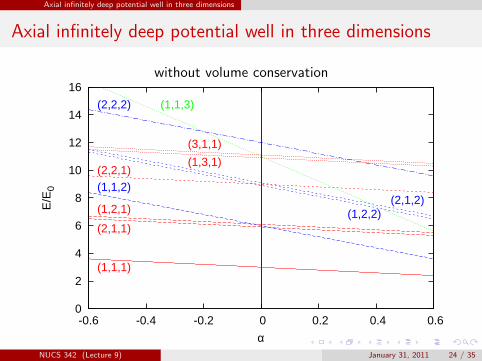
Axial infinitely deep potential well in three dimensions
Axial infinitely deep potential well in three dimensions
without volume conservation
0
2
4
6
8
10
12
14
16
-0.6 -0.4 -0.2 0 0.2 0.4 0.6
E/E
0
α
(1,1,1)
(2,1,1)
(1,2,1)
(2,2,1)(1,3,1)
(3,1,1)
(1,1,2)
(1,2,2)(2,1,2)
(2,2,2) (1,1,3)
NUCS 342 (Lecture 9) January 31, 2011 24 / 35
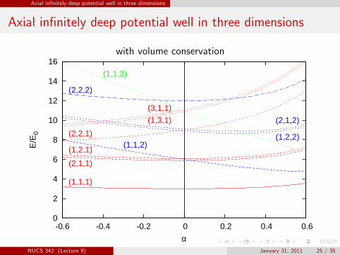
Axial infinitely deep potential well in three dimensions
Axial infinitely deep potential well in three dimensions
with volume conservation
0
2
4
6
8
10
12
14
16
-0.6 -0.4 -0.2 0 0.2 0.4 0.6
E/E
0
α
(1,1,1)
(2,1,1)
(1,2,1)
(2,2,1)
(1,3,1)
(3,1,1)
(1,1,2)(1,2,2)
(2,1,2)
(2,2,2)
(1,1,3)
NUCS 342 (Lecture 9) January 31, 2011 25 / 35
Axial infinitely deep potential well in three dimensions
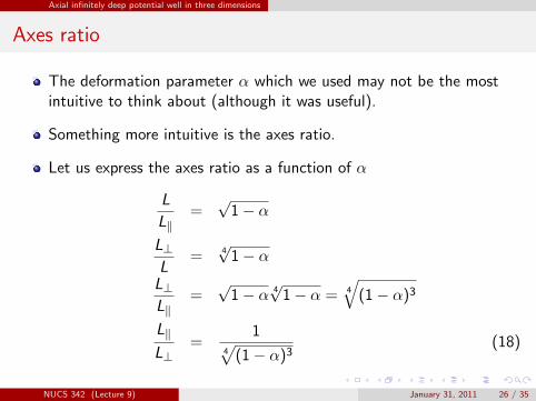
Axes ratio
The deformation parameter α which we used may not be the mostintuitive to think about (although it was useful).
Something more intuitive is the axes ratio.
Let us express the axes ratio as a function of α
L
L‖=√
1− α
L⊥L
= 4√
1− α
L⊥L‖
=√
1− α 4√
1− α = 4
√(1− α)3
L‖L⊥
=1
4√
(1− α)3(18)
NUCS 342 (Lecture 9) January 31, 2011 26 / 35
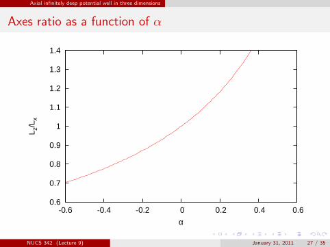
Axial infinitely deep potential well in three dimensions
Axes ratio as a function of α
0.6
0.7
0.8
0.9
1
1.1
1.2
1.3
1.4
-0.6 -0.4 -0.2 0 0.2 0.4 0.6
L z/L
x
α
NUCS 342 (Lecture 9) January 31, 2011 27 / 35
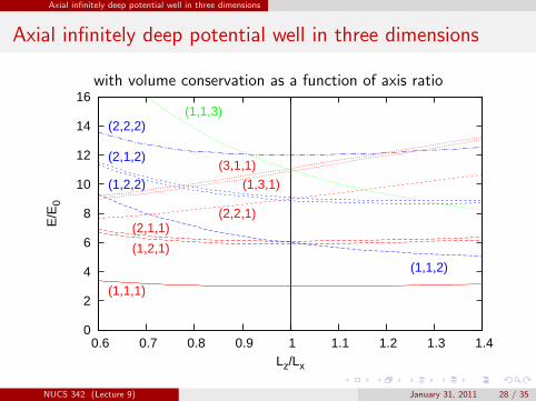
Axial infinitely deep potential well in three dimensions
Axial infinitely deep potential well in three dimensions
with volume conservation as a function of axis ratio
0
2
4
6
8
10
12
14
16
0.6 0.7 0.8 0.9 1 1.1 1.2 1.3 1.4
E/E
0
Lz/Lx
(1,1,1)
(2,1,1)
(1,2,1)
(2,2,1)
(1,3,1)
(3,1,1)
(1,1,2)
(1,2,2)
(2,1,2)
(2,2,2)(1,1,3)
NUCS 342 (Lecture 9) January 31, 2011 28 / 35
The Nilsson model
The Nilsson model
What we have done for the three dimensional potential well has beendone with a great success for nuclear harmonic oscillator potential in3 dimensions including the flat bottom correction and spin-orbit termsto model deformed nuclear potential
The deformed shell model he developed is often referred to as theNilsson model.
As for the three dimensional potential well the Nilsson model predictsthat shells and shell gaps are modified by the deformation.
The main achievement of the Nilsson model is correct explanation ofground state spins and parities of a large number of nuclei, as well itsability to be expanded into a model for rotation of deformedodd-mass nuclei (later this week).
NUCS 342 (Lecture 9) January 31, 2011 29 / 35
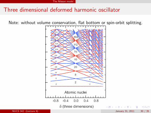
The Nilsson model
Three dimensional deformed harmonic oscillator
Note: without volume conservation, flat bottom or spin-orbit splitting.
NUCS 342 (Lecture 9) January 31, 2011 30 / 35
The Nilsson model
The total angular momentum in Nilsson model
One of the consequence of deformation is configuration mixing. Forexample the d5/2 and the d3/2 states which are separate for thespherical shell model mix in the Nilsson model.
As a consequence of mixing the total angular momentum does nothave a well defined value in a deformed shell model, for example for amixture of d5/2 and the d3/2 states the total angular momentum is a
mixture of j = 52 and j = 3
2
However, in the axially-symmetric Nilsson model deformation theprojection of the total angular momentum on the symmetry axis(analogues to the magnetic m-quantum number) has a well definedhalf-integer value.
This quantum number in the Nilsson model is referred to as Ω.
NUCS 342 (Lecture 9) January 31, 2011 31 / 35
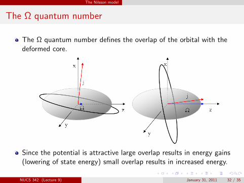
The Nilsson model
The Ω quantum number
The Ω quantum number defines the overlap of the orbital with thedeformed core.
Since the potential is attractive large overlap results in energy gains(lowering of state energy) small overlap results in increased energy.
NUCS 342 (Lecture 9) January 31, 2011 32 / 35
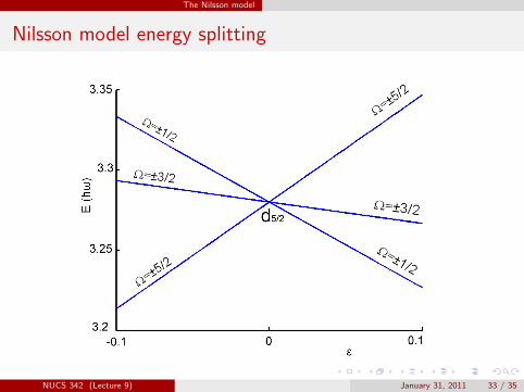
The Nilsson model
Nilsson model energy splitting
NUCS 342 (Lecture 9) January 31, 2011 33 / 35
The Nilsson model
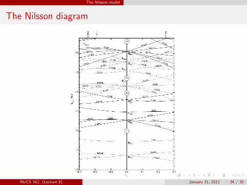
The Nilsson diagram
NUCS 342 (Lecture 9) January 31, 2011 34 / 35
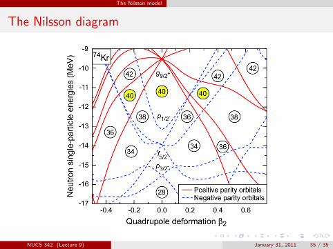
The Nilsson model
The Nilsson diagram
NUCS 342 (Lecture 9) January 31, 2011 35 / 35