defra / environment agency flood and coastal defence r&d ... · defra / environment agency...
TRANSCRIPT
Defra / Environment AgencyFlood and Coastal Defence R&D Programme
Reducing uncertainty in river flood conveyance, Phase 2
Conveyance Manual
Project Record W5A-057/PR/1
Defra / Environment AgencyFlood and Coastal Defence R&D Programme
REDUCING UNCERTAINTY IN RIVER FLOODCONVEYANCE, PHASE 2
Conveyance Manual
Project Record W5A-057/PR/1
Research Contractor: HR Wallingford
R&D OUTPUTS: CONVEYANCE USER MANUAL- ii -
Publishing organisationEnvironment Agency, Rio House, Waterside Drive, Aztec West, Bristol BS32 4UDTel: +44 (0)1454 624400 Fax: +44 (0)1454 624409 Web: www.environment-agency.gov.uk© Environment Agency September 2004 Product Code: SCHO0904BIHR-E-EISBN: 1844323048
The Environment Agency will waive its normal copyright restrictions, and allow this document(or other item), excluding the logo to be reproduced free of licence or royalty charges in anyform, provided that it is reproduced unaltered in its entirety and its source acknowledged asEnvironment Agency copyright.
This waiver is limited to this document (or other item) and is not applicable to any otherEnvironment Agency copyright material, unless specifically stated. The Environment Agencyaccepts no responsibility whatever for the appropriateness of any intended usage of thedocument, or for any conclusions formed as a result of its amalgamation or association with anyother material.
The views expressed in this document are not necessarily those of Defra or the EnvironmentAgency. Its officers, servants or agents accept no liability whatsoever for any loss or damagearising from the interpretation or use of the information, or reliance on views contained herein.
Dissemination StatusInternal: Released to Regions and AreasExternal: Released to Public Domain
Statement of useThis document provides support and training for users of the Conveyance Estimation Systemsoftware, the core output for R&D Project W5A-057.
KeywordsConveyance principles, river flow, numerical model, software training, worked examples
Contract DetailsThe lead funder for this collaborative project was the Defra / EA Joint Flood and CoastalDefence R&D Programme. Scottish Executive, Rivers Agency – Northern Ireland, and theNatural Environment Research Council also contributed funding. Wallingford Softwaresupported the development of new software.
Research ContractorThis document was produced under R&D Project W5A-057 byHR Wallingford Ltd, Howbery Park, Wallingford, Oxon OX10 8BA, supported by an expertadvisory group (Professors Garry Pender, Alan Ervine and Donald Knight plus Dr ChrisWhitlow).
Tel: +44 (0)1491 835381 Fax: +44 (0) 1491 832233 Web: www.hrwallingford.co.uk.Contractor’s Project Manager: Manuela Escarameia
Environment Agency's Project ManagerThe Environment Agency's Project Manager: Dr Mervyn Bramley, Engineering Theme Leader
This report is only available in electronic form over the Defra / Environment Agencywebpages for the Joint Flood and Coastal Erosion Risk Management R&D Programme.
R&D OUTPUTS: CONVEYANCE USER MANUAL- iii -
ABBREVIATIONS
CES Conveyance Estimation System
CG Conveyance Generator
DCM Divided Channel Method
DEFRA Department for Environment, Food and Rural Affairs
EA Environment Agency
FCF Flood Channel Facility
IDB Internal Drainage Boards
LiDar Airborne scanning Laser Altimetry
MDSF Modelling and Decision Support Framework
OS Ordnance Survey
RA Roughness Advisor
RANS Reynolds-Averaged Navier-Stokes
RASP Risk Assessment of Flood and Coastal Defence Systems for StrategicPlanning
RHS River Habitat Survey
SAR Sonar Acoustique Remorque
SP Strategic Programme
TP Targeted Programme
UE Uncertainty Estimator
UK United Kingdom
1D One Dimensional

R&D OUTPUTS: CONVEYANCE USER MANUAL- iv -
R&D OUTPUTS: CONVEYANCE USER MANUAL- v -
SYMBOLS
Latin Alphabet
C Chezy coefficient (m0.5.s-1)Cuv coefficient for sinuosityDr relative depth = h/Hmax (m.m-1)E specific energy (m)f local boundary friction factor based on the local substrate/vegetation roughnessg gravitational acceleration (m.s-2)H local water depth normal to the bed (m)Hmax maximum depth for a given channel section (m)h water surface level (m)�hc uncertainty in water level due to calibration�hq uncertainty in water level due to hydrology�hr uncertainty in water level due to roughness�hs uncertainty in water level due to survey data�hu total uncertainty in water level�h�x uncertainty in water level due to numerical considerations e.g. grid resolutionK cross-sectional channel conveyance (m3.s-1)k unit conveyance (m2.s-1)ks absolute roughness height (m)n Manning’s roughness coefficient (s.m-1/3)ne engineering ‘n’ which is all encompassing (s.m-1/3)nirr unit roughness component due to irregularities (s.m-1/3)nl local ‘n’ includes local boundary friction losses only (s.m-1/3)nsur unit roughness component due to surface material (s.m-1/3)nveg unit roughness component due to vegetation (s.m-1/3)Q total cross-section discharge (m3.s-1)q unit flow rate (m2.s-1)S common uniform gradientSf streamwise friction or ‘specific energy’ gradientSo reach-averaged longitudinal bed slopeT fluid temperature (�C)u streamwise point velocity (m.s-1)U section average velocity (m.s-1) in Section 2.3.1Ud depth-averaged streamwise velocity (m.s-1) (RANS approach)U* shear velocity (m.s-1)U streamwise velocity component at a given depth (m.s-1)Vd depth-averaged lateral velocity (m.s-1) (RANS approach)V lateral velocity component at a given depth (m.s-1))x streamwise direction parallel to the bed (m)y lateral distance across section (m) (RANS approach)z measured perpendicular to the channel bed (m)
Greek alphabet
� coefficient for the influence of lateral and longitudinal bed slope on the bedshear stress

R&D OUTPUTS: CONVEYANCE USER MANUAL- vi -
� secondary flow term for straight prismatic channels�fp secondary flow term for floodplain flows�mci secondary flow term for main channel inbank flows�mco secondary flow term for main channel out-of-bank flows� dimensionless eddy viscosity�mc main channel dimensionless eddy viscosity� kinematic viscosity of the fluid (m2.s-1)� sinuosity - thalweg length over the valley length (m.m-1)� fluid density (kg.m-3)�b bed shear stress (N.m-2) relaxation factor
R&D OUTPUTS: CONVEYANCE USER MANUAL- vii -
GLOSSARY OF TERMS
Accuracy: Accuracy has two facets. It deals with the precision to whichmeasurement or calculation is carried out (i.e. the maximumdeviation of the measurement or calculation from the “true”amount) and with the number of digits of precision which arecarried through a calculation (whether or not these aremeaningful). Potentially, accuracy can be improved bybetter technology.
Backwater: Backwater effects occur when sub-critical flow is controlledby the downstream conditions e.g. presence of an outfall,bridge constriction, dam etc.
Bankfull: The maximum channel discharge capacity; further dischargespreads onto the floodplains.
Berms: (i) The space left between the upper edge of a cut and toe ofan embankment to break the continuity of an otherwise longslope.(ii) The sharp definitive edge of a dredged channel such as ina rock cut.(iii) Natural levee where river deposits sediment
Braided channel: A channel that is divided into two or more channels e.g. flowaround an island.
Conveyance: Channel conveyance is a measure of the discharge carrying
capacity of a channel K m3/s, defined as K2
1
fS
Q�
Eddy viscosity: Parameter representing the momentum exchange, (m2/s),defined in the CES methodology (DEFRA/EA, 2003a) as
DU*�� which relates viscosity to the bed shear stresses.
Dimensionless eddyviscosity:
Calibration coefficient to account for lateral shear �
Discharge: The volume of water that passes through a channel sectionper unit time.
Error: Errors are mistaken calculations or measurements withquantifiable and predictable differences from the actualvalue.
Flow: A general term for the movement of volumes of water at aspeed.
Flow zone: Area in a channel cross-section within which the flowcharacteristics represent a particular flow mechanism or
R&D OUTPUTS: CONVEYANCE USER MANUAL- viii -
selection of mechanisms e.g. secondary flow, shearing flowetc. (This is different to a roughness zone.)
Irregularity: Channel irregularities represent variations in roughness fromobstructions such as exposed boulders, trash, groynes etc orchannel shape e.g. pools and riffles.
Manning’s ne: An empirical coefficient ne that lumps together all losses i.e.losses due to local friction, secondary flows, form losses andlateral shear stresses (Chow, 1959). Derived for use inmedium to large non-vegetated rivers with fully developedflow profiles.
Manning’s pure nl: A coefficient that approximates the local friction losses dueto bed features only i.e. surface material, vegetation and / orirregularities.
Maximum depth: The vertical distance of the lowest point of a channel sectionfrom the free water surface
Morpho-types: See “vegetation morpho-types”
Multi-thread channel: A channel that is divided into two or more channels e.g. flowaround an island.
Offset: Distance measured laterally across the channel, taken fromthe left-hand side when looking downstream.
RANS: The Navier-Stokes equations are derived from the governingequations of fluid flow. These equations are termed“Reynolds Averaged” as the instantaneous turbulentfluctuations of the velocity and pressure components havebeen averaged over small time-scales i.e. small comparedwith variations in the bulk flow that are of any practicalimportance, but large compared with inter-particle collisions.The “Reynolds Averaged” Navier-Stokes equations are100% based on modelling of the physical properties.
Resistance: As for roughness but defined as flow-, form-, frictional orturbulent etc
Reynolds Number: The Reynolds Number describes the ratio of the inertiaforces to the viscous forces (Re = 4Rv/� and R is thehydraulic radius). In open channel flow, for Re < 500laminar flow occurs, Re > 1000, turbulent flow occurs andfor 500 < Re < 1000 transitional flow occurs, i.e. the flow ischaracterised by both laminar and turbulent effects.
Riffle: A point at which the stream is relatively energetic due to aconstriction or steep gradient (the counterpart of pool).
R&D OUTPUTS: CONVEYANCE USER MANUAL- ix -
Roughness: The effect of impeding the normal water flow of a channelby the presence of a natural or artificial body or bodies,biotic e.g. vegetation; abiotic / mineral e.g. bank, bedsubstrate.
Roughnesscomponents:
A roughness component is a category of unit roughness thatmay be vegetation, surface material or irregularity. All unitroughness values fall into one of these three components.
Roughness types: The roughness type refers to the portion of the cross-sectionwhere a particular surface cover is likely to be found e.g.crops on the floodplain. There are three roughness types:bed, bank and floodplain.
Roughness zones: A roughness zone is a plan area in the river/floodplainsystem that is characterised by similar roughness e.g. a field,bank vegetation, crops with clay below etc. A roughnesszone can only be comprised of three roughness components.
Sinuosity: A measure of a channel’s tendency to meander defined in theCES as thalweg length over valley length.
Stage: The vertical distance of the free surface from an arbitrary ordefined datum
Study reach: The length of a study reach OR a section under investigation/measurement
Substrate: A generic term for a substance that underlies another; soil isthe substrate for plants, while bedrock is the substrate forsoil.
Surface material: Surface material encompasses the substrate on the bed, bankand floodplains. The roughness due to surface materialincludes for e.g. sand, gravel, peat, rock etc.
Thalweg: A line connecting the deepest points along a channel length
Top-of-bank bendmarkers:
The top-of-bank bend markers are top-of-bank markers formeandering channels. They are used to determine theorientation of the bend through specifying them as inside oroutside of bend.
Top-of-bank markers: Top-of-bank markers are used to incorporate the changes insecondary flow mechanisms at bankfull into the conveyancecalculation. These are placed on the cross-section at theintersection between the main channel and floodplain.
Turbulence: Turbulent flow occurs at high Reynolds Number (Re > 1000for open channel flow) when the flow incorporates an
R&D OUTPUTS: CONVEYANCE USER MANUAL- x -
eddying or mixing action, and the inertia forces dominate theviscous forces. A chaotic and random state of motiondevelops in which the velocity and pressure changescontinuously with time, within substantial regions of flow.The fluid particles are therefore continuously interchangingand it follows that the fluid properties may be exchanged.The crucial difference between visualisations of laminar andturbulent flows is the appearance of eddies on a wide rangeof length scales in the turbulent flows.
Uncertainty: Uncertainty comprises (i) natural variability and (ii)knowledge uncertainty. It arises principally from lack ofknowledge or that of ability to measure or to calculate whichgives rise to potential differences between assessment ofsome factor and its “true” value.
Unit conveyance: Conveyance per metre width of channel k (m2/s), defined as
k2
1
fS
q� .
Unit discharge: Flow rate per metre width of channel section q (m2/s),
defined as q dzuH
��
0
.
Unit roughness: Roughness due to an identifiable segment of boundaryfriction per unit length of channel.
Vegetation Morpho-types:
These are aquatic and marginal plant species of similar formor function in the riparian corridor. These are not vegetationtypes with similar morphological character.
R&D OUTPUTS: CONVEYANCE USER MANUAL- xi -
SUMMARY
Under their joint R&D programme for Flood and Coastal Defence, Defra/EnvironmentAgency have funded a Targeted Programme of research aimed at obtaining betterpredictions of flood water levels. In order to achieve this, advances in knowledge andunderstanding made over the past three or four decades in the estimation of riverconveyance are being introduced into engineering practice.
The project relates particularly to water level estimation, leading to a reduction in theuncertainty in the prediction of flood levels and hence in flood risk, and consequentlyfacilitating better targeting of expenditure. The project will equally benefit the targetingof maintenance by providing better estimates of the effects of vegetation and itsmanagement. It is expected that the application of this knowledge from UK engineeringresearch will have an international impact through improving the methods available toconsultants.
The above objectives will be achieved through three core components of the newConveyance Estimation System (CES): the Conveyance Generator, the RoughnessAdvisor and the Uncertainty Estimator. A Backwater Module is also available. TheCES is designed so that new knowledge from a parallel Strategic Programme ofresearch can be integrated into the CES in due course.
The Conveyance Manual provides a guide for the Conveyance Estimation Systemsoftware, covering the technical background, user application and providing workedexamples. The Manual is intended to assist the user in the hands-on application of thesoftware, providing advice where subjective decisions are required and assisting ininterpretation of results. It includes an additional section on the advanced user optionsand the Backwater Module.

R&D OUTPUTS: CONVEYANCE USER MANUAL- xii -

R&D OUTPUTS: CONVEYANCE USER MANUAL- xiii -
CONTENTS
ABBREVIATIONS iiiSYMBOLS vGLOSSARY OF TERMS viiSUMMARY iii
1. Introduction 11.1 Why do we need a new conveyance system? 1
1.2 What is the CES? 1
1.3 Why Provide a Conveyance Manual? 2
1.4 How do I use the Conveyance Manual effectively? 2
2. Technical Background 32.1 Overview 3
2.1.1 What are legacy practices in conveyance estimation? 32.1.2 What changes are expected after the CES is recognised as the
industry norm? 32.1.3 What will I do that I did not do in legacy practices? 42.1.4 What will the CES do? 42.1.5 What new opportunities are provided by the CES? 4
2.2 Roughness 52.2.1 Why do we need to worry about roughness? 52.2.2 Why is there a need for a new approach to estimating roughness? 52.2.3 How is the roughness represented? 62.2.4 What is a unit roughness nl-value? 62.2.5 Why was the decision taken to express roughness in terms of ‘n’? 62.2.6 What is a roughness component? 62.2.7 How are the component roughness values combined? 6
2.3 Conveyance 72.3.1 What is conveyance? 72.3.2 Why do we need to know about channel conveyance? 82.3.3 Why is there a new approach for estimating channel conveyance? 82.3.4 Do I need to have a strong mathematical background to use the CES? 92.3.5 What are the different energy loss mechanisms? 92.3.6 What is the selected approach in the CES for calculating conveyance? 112.3.7 Why was the RANS approach selected? 152.3.8 What are the limitations of this method? 162.3.9 How are the RANS equations solved? 172.3.10 How is my cross-section discretised? 172.3.11 Has this approach been tested? 17
2.4 Uncertainty 182.4.1 What is uncertainty? 182.4.2 Why do I need to account for uncertainty? 182.4.3 What factors contribute to the uncertainty in conveyance? 192.4.4 What approaches for estimating uncertainty were considered? 20

R&D OUTPUTS: CONVEYANCE USER MANUAL- xiv -
2.4.5 How is uncertainty represented in the CES? 232.4.6 How is the uncertainty calculated in the CES? 252.4.7 What are the dominant factors that are considered? 262.4.8 Why was this approach selected? 262.4.9 What is the effect of calibration? 27
2.5 Backwater 272.5.1 What is a backwater profile? 272.5.2 Why do I need to know about backwater effects? 272.5.3 How is the backwater calculated? 282.5.4 What are the Backwater method restrictions? 29
3. Using the CES 313.1 Roughness advisor 31
3.1.1 What is the Roughness Advisor? 313.1.2 What will the Roughness Advisor provide? 313.1.3 What is a roughness zone type? 313.1.4 What is a roughness zone? 313.1.5 Why do I specify roughness zones? 323.1.6 How do I get the roughness values in the Roughness Advisor? 323.1.7 Can I put my own roughness values in? 323.1.8 Are there minimum and maximum allowable unit roughness values? 333.1.9 What are the seasonal variations in vegetation? 333.1.10 How are the cutting regimes used? 33
3.2 Conveyance Generator 333.2.1 How do I describe the cross-section geometry? 333.2.2 How do I represent the roughness zones in my cross-section
geometry? 343.2.3 Does the channel cross-section represent the start or mid-point of the
channel reach? 353.2.4 What are the top-of-bank markers used for? 353.2.5 Do I have to use top-of-bank markers? 363.2.6 Where should top-of-bank markers be positioned? 363.2.7 How do I model meandering channels? 383.2.8 How do I label top-of-bank bend markers on skewed channels? 393.2.9 How do I calculate the channel sinuosity? 403.2.10 What are typical UK channel sinuosities? 403.2.11 How do I model braided channels? 423.2.12 How do I model braided channels with different sinuosity values? 433.2.13 How do I model non-conveyance storage zones i.e. zones with re-
circulation or stationary water? 443.2.14 What is the range of depths for which the conveyance is calculated? 443.2.15 Are there any special survey requirements for application of the
CES? 443.2.16 What slope do I use? 45
3.3 Uncertainty Estimator 453.3.1 How is uncertainty represented in the CES? 453.3.2 How should this uncertainty information be interpreted? 453.3.3 How should this uncertainty information be used? 463.3.4 How ‘certain’ is the uncertainty calculation? 47
R&D OUTPUTS: CONVEYANCE USER MANUAL- xv -
3.3.5 How do I ensure the uncertainty is calculated? 47
3.4 Calibration and interpretation of results 483.4.1 How do I calibrate my model and what do I change when the data
does not fit? 483.4.2 Why do I get jumps in the conveyance curve at sudden geometry
changes e.g. bankfull? 483.4.3 Why do I sometimes get large jumps at bankfull depth for high
sinuosities? 493.4.4 Why are the uncertainty curves not symmetrical about the expected
value? 503.4.5 Why is the uncertainty greater at small depths? 50
3.5 Advanced Options 503.5.1 Do I need to alter the advanced options? 503.5.2 What effect will increasing the number of depths have? 513.5.3 What effect will increasing the number of lateral divisions have? 513.5.4 What happens if I change the dimensionless eddy viscosity? 523.5.5 What happens if I change the straight secondary flow coefficients? 523.5.6 What happens if I alter the temperature? 523.5.7 What happens if I alter the relaxation parameter? 523.5.8 If I alter an advanced parameter, does the change apply to that cross-
section only? 533.5.9 What happens if I set the minimum depth? 533.5.10 Why would I set the minimum depth? 533.5.11 What does the wall height multiplier do? 533.5.12 What happens if I alter the maximum number of iterations? 533.5.13 What does the experimental flume option change? 533.5.14 What does the convergence tolerance change? 53
3.6 Backwater Module 543.6.1 How is the backwater module used? 543.6.2 What Backwater options are available? 543.6.3 What is the advantage of using the backwater module compared to a
complete 1D modelling software such as iSIS or MIKE 11? 54
4. Worked examples 554.1 Worked example of the River Main, Northern Ireland 55
4.1.1 Available user information 55
4.2 Using the Roughness Advisor to generate roughness zones 574.2.1 Using the Conveyance Generator to generate a rating curve 634.2.2 Calibrating process (depends on data availability) 694.2.3 Final result and interpretation of uncertainty 69
4.3 Worked example of the River Blackwater 694.3.1 Available user information 694.3.2 Using the Roughness Advisor to generate roughness zones 724.3.3 Using the Conveyance Generator to generate a rating curve 764.3.4 Calibrating process (depends on data availability) 804.3.5 Final result and interpretation of uncertainty 80
4.4 Worked example of River Dane 81
R&D OUTPUTS: CONVEYANCE USER MANUAL- xvi -
4.4.1 Available user information 814.4.2 Using the Roughness Advisor to generate roughness zones 834.4.3 Using the Conveyance Generator to generate a rating curve 874.4.4 Calibrating process (depends on data availability) 894.4.5 Final result and interpretation of uncertainty 90
5. References 91
TablesTable 2.1 Potential consequences of uncertainty in flood conveyance 19
Table 2.2 Summary of Uncertainty users and their needs 24
Table 2.3 Backwater lengths for some UK Rivers (Samuels, 1989) 28
Table 3.1 Use of uncertainty information for different user groups 46
Table 3.2 Allowable ranges for the advanced options 51
Table 4.1 River Main cross-section 14 geometry 56
Table 4.2 Final Roughness Advisor (.rad file) output for the River Main 63
Table 4.3 River Blackwater cross-section geometry 71
Table 4.4 Final Roughness Advisor (.rad file) output for the River Blackwater 76
Table 4.5 River Dane cross-section 30 Geometry 83
FiguresFigure 2.1 Example of components for substrate and vegetation contributing to
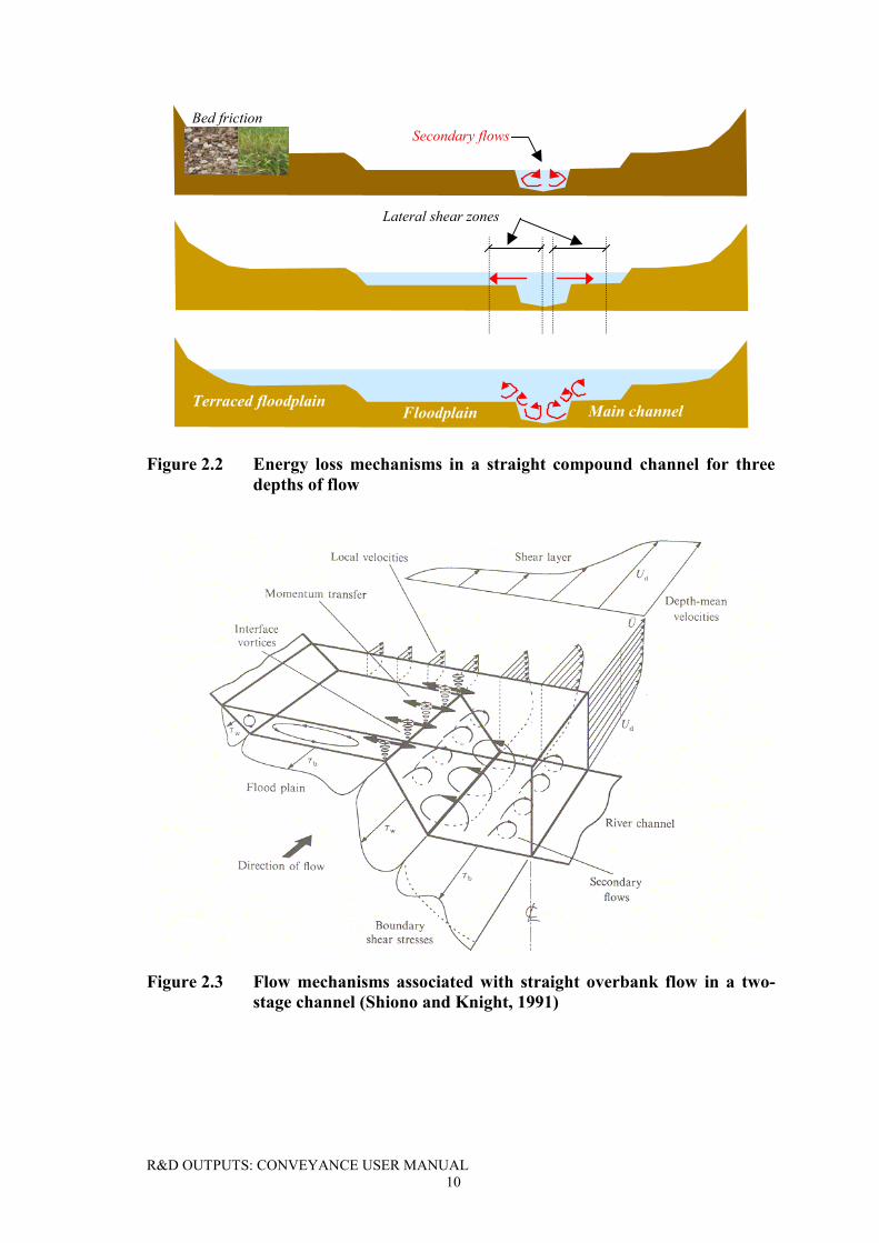
local boundary friction 7Figure 2.2 Energy loss mechanisms in a straight compound channel for three
depths of flow 10
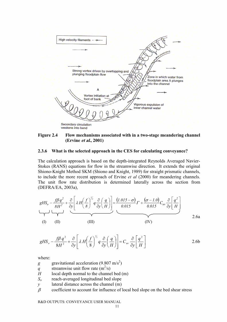
Figure 2.3 Flow mechanisms associated with straight overbank flow in a two-stagechannel (Shiono and Knight, 1991) 10
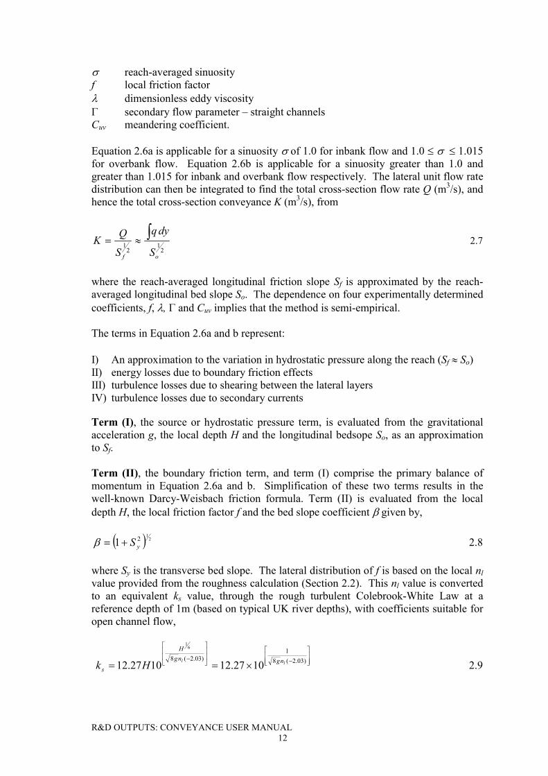
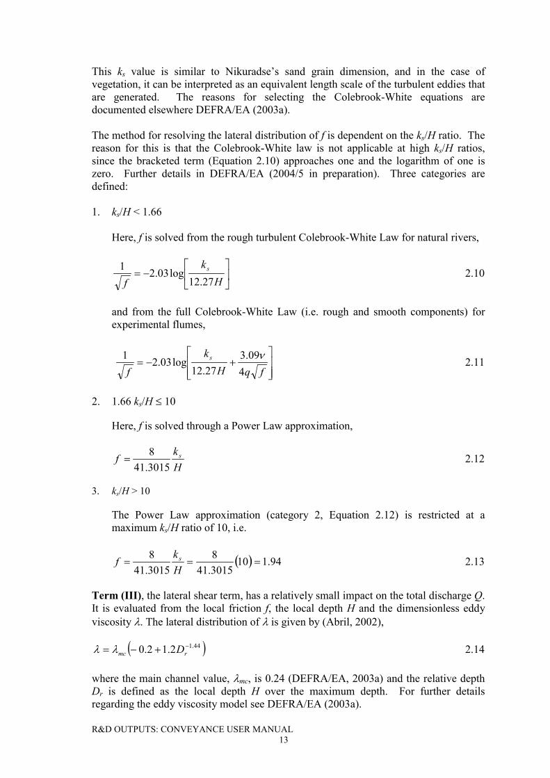
Figure 2.4 Flow mechanisms associated with in a two-stage meandering channel(Ervine et al., 2001) 11
Figure 2.5 Contributions from the secondary flow terms with increasing sinuosity 14
Figure 2.6 Lateral distribution of calibration parameters for a typical two-stagechannel 15
Figure 2.7 Cross-section discretisation 17
Figure 2.8 Upper and lower uncertainty bands in the RASP analysis 21
Figure 2.9 The Monte Carlo approach 23
Figure 2.10 Representation of uncertainty for a rating curve 25
Figure 2.11 Effect of calibration 27
Figure 2.12 Backwater calculation method from cross-section 1 to 3 29
R&D OUTPUTS: CONVEYANCE USER MANUAL- xvii -
Figure 3.1 Plan view of roughness zones 32
Figure 3.2 Example of cross-sections that cannot be modelled within theConveyance Generator 34
Figure 3.3 Setting extreme / edge co-ordinates with maximum values as afunction of maximum depth 34
Figure 3.4 Cross-sections with the lateral distribution of roughness zones 35
Figure 3.5 Variation of secondary flow term for straight channels 35
Figure 3.6 Variation of secondary flow term for floodplains with differentelevations 36
Figure 3.7 Positioning of top-of-bank markers for single channels and isolatedfloodplains 36
Figure 3.8 Positioning of top-of-bank markers for asymmetric channels 37
Figure 3.9 Positioning of top-of-bank markers for channels with berms 37
Figure 3.10 Top-of-bank markers for low elevation floodplains 38
Figure 3.11 Typical observed depth-averaged velocity profiles in meanderingchannels and top-of bank bend marker positions 39
Figure 3.12 Top-of-bank markers for skewed channels 40
Figure 3.13 Definition sketch for sinuosity 40
Figure 3.14a Sinuosity values for (a) the Flood Channel Facility at HR Wallingford,(b) the Glasgow University small-scale flume, (c) the River Dane inCheshire, (d) Kleinschmidt Creek (Photo courtesy of Land and WaterConsulting), (e) incised meanders, Utah and (b) Wood River, SouthernNebraska 41
Figure 3.14b Plan view of channels with increasing sinuosity 42
Figure 3.15 Addition of flow in braided channels (DEFRA/EA, 2003a) 42
Figure 3.16 Top-of-bank markers for a braided channel 42
Figure 3.17 Top-of-bank marker positions for deep flow in a braided channel 43
Figure 3.18 Top-of-bank bend markers for multi-thread channels with differentsinuosities 43
Figure 3.19 Top-of-bank bend and straight markers for multi-thread channels withdifferent sinuosities 43
Figure 3.20 Non-conveyance zone specification – single units only 44
Figure 3.21 Unusual ‘jumps’ in stage-discharge curves reflect observed data e.g.River Severn, Montford 49
Figure 3.22 Discontinuity in stage-discharge curves in meandering channels reflectthe observed data e.g. Flood channel Facility Phase B20/21 observations50
Figure 4.1 River Main in County Antrim, Northern Ireland (a) the side-banks withrip-rap and (b) a gentle meander 55
Figure 4.2 Plan view of the River Main indicating the selected cross-section 14 56
R&D OUTPUTS: CONVEYANCE USER MANUAL- xviii -
Figure 4.3 River Main cross-section 14 geometry 57
Figure 4.4 Create a new roughness file 57
Figure 4.5 Create three roughness zones: bed cover, bank cover and floodplaincover 58
Figure 4.6 Providing roughness zone description: Coarse gravel 58
Figure 4.7 Three roughness component options 59
Figure 4.8 Bed material component with gravel selected 59
Figure 4.9 Bed material component now populated 60
Figure 4.10 Providing roughness zone description: Rip-rap 60
Figure 4.11 Bank material component with rip-rap selected 61
Figure 4.12 Providing roughness zone description: Heavy weed growth 61
Figure 4.13 Floodplain ground material component with height varying grassselected 62
Figure 4.14 Floodplain ground material component with sand selected 62
Figure 4.15 Create a new conveyance file 63
Figure 4.16 Select River Main roughness file 63
Figure 4.17 Cross-section description 64
Figure 4.18 Select ‘properties’ for the now populated first cross-section 64
Figure 4.19 Cross-section data for cross-section 14 65
Figure 4.20 Roughness zone allocation 66
Figure 4.21 The River Main rating curve for Section 14 67
Figure 4.22 Comparison of the CES stage-discharge prediction to the measured data 67
Figure 4.23 Alter the number of calculation depths in the Advanced Options 68
Figure 4.24 Improved CES prediction from increasing the number of depths inAdvanced Options 68
Figure 4.25 Upper and lower uncertainty bands for the conveyance calculation 69
Figure 4.26 Vegetation on the River Blackwater (Hampshire, UK) in (a) May 1996downstream from Colebrook Bridge (b) March 1995 downstream fromColebrook Bridge and (c) May 1996 upstream from the footbridge 70
Figure 4.27 Plan view of the River Blackwater indicating Gauge site 3 71
Figure 4.28 River Blackwater cross-section geometry – Gauge site 3 72
Figure 4.29 Roughness zones and descriptions for the River Blackwater 72
Figure 4.30 Select time series for the submerged fine-leaved plants 73
Figure 4.31 Expected time series for the submerged fine-leaved plants (0.6-1.2mdepth) 74
Figure 4.32 Bed cover zone unit roughness values 74
Figure 4.33 Emergent reeds characteristic of the bank vegetation 75
R&D OUTPUTS: CONVEYANCE USER MANUAL- xix -
Figure 4.34 Roughness zones for the River Blackwater 75
Figure 4.35 Cross-section details for Gauge site 3 on the River Blackwater 76
Figure 4.36 River Blackwater cross-section at Gauge site 3 illustrating the leftinside of bend top-of-bank marker 77
Figure 4.37 River Blackwater roughness zone allocation 78
Figure 4.38 Select the date for the CES conveyance prediction 78
Figure 4.39 Comparison of the CES predicted conveyance to the measured data forFebruary 1995 79
Figure 4.40 Comparison of the CES predicted conveyance to the measured data forJune 1995 79
Figure 4.41 Comparison of the CES predicted conveyance to the measured data forDecember 1999 80
Figure 4.42 The conveyance predictions for Gauge site 3 on the River Blackwaterwith the uncertainty bands shown 81
Figure 4.44 River Dane vegetation 81
Figure 4.43 The 6km reach of the River Dane with cross-section 30 identified 82
Figure 4.45 River Dane cross-section 30 geometry 83
Figure 4.46 Roughness zone definition and description 84
Figure 4.47 Select the Time series for emergent reeds 85
Figure 4.48 Emergent reed time series for a given year 85
Figure 4.49 Manually overwrite the suggested roughness based on availableinformation 86
Figure 4.50 Final roughness zone value in the .rad file 86
Figure 4.51 River Dane channel description 87
Figure 4.52 River Dane cross-section with straight top-of-bank markers 87
Figure 4.53 River Dane roughness zone allocation 88
Figure 4.54 River Dane CES rating curve prediction compared to the measured data 89
Figure 4.55 The River Dane stage-discharge curve after calibration 90
Figure 4.56 Final stage-discharge curve for the River Dane 90

R&D OUTPUTS: CONVEYANCE USER MANUAL- xx -
R&D OUTPUTS: CONVEYANCE USER MANUAL1
1. INTRODUCTION
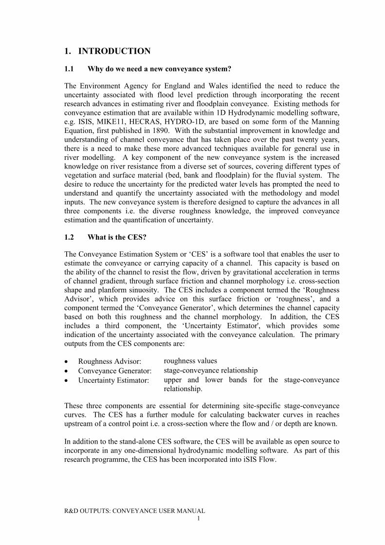
1.1 Why do we need a new conveyance system?
The Environment Agency for England and Wales identified the need to reduce theuncertainty associated with flood level prediction through incorporating the recentresearch advances in estimating river and floodplain conveyance. Existing methods forconveyance estimation that are available within 1D Hydrodynamic modelling software,e.g. ISIS, MIKE11, HECRAS, HYDRO-1D, are based on some form of the ManningEquation, first published in 1890. With the substantial improvement in knowledge andunderstanding of channel conveyance that has taken place over the past twenty years,there is a need to make these more advanced techniques available for general use inriver modelling. A key component of the new conveyance system is the increasedknowledge on river resistance from a diverse set of sources, covering different types ofvegetation and surface material (bed, bank and floodplain) for the fluvial system. Thedesire to reduce the uncertainty for the predicted water levels has prompted the need tounderstand and quantify the uncertainty associated with the methodology and modelinputs. The new conveyance system is therefore designed to capture the advances in allthree components i.e. the diverse roughness knowledge, the improved conveyanceestimation and the quantification of uncertainty.
1.2 What is the CES?
The Conveyance Estimation System or ‘CES’ is a software tool that enables the user toestimate the conveyance or carrying capacity of a channel. This capacity is based onthe ability of the channel to resist the flow, driven by gravitational acceleration in termsof channel gradient, through surface friction and channel morphology i.e. cross-sectionshape and planform sinuosity. The CES includes a component termed the ‘RoughnessAdvisor’, which provides advice on this surface friction or ‘roughness’, and acomponent termed the ‘Conveyance Generator’, which determines the channel capacitybased on both this roughness and the channel morphology. In addition, the CESincludes a third component, the ‘Uncertainty Estimator', which provides someindication of the uncertainty associated with the conveyance calculation. The primaryoutputs from the CES components are:
� Roughness Advisor: roughness values� Conveyance Generator: stage-conveyance relationship� Uncertainty Estimator: upper and lower bands for the stage-conveyance
relationship.
These three components are essential for determining site-specific stage-conveyancecurves. The CES has a further module for calculating backwater curves in reachesupstream of a control point i.e. a cross-section where the flow and / or depth are known.
In addition to the stand-alone CES software, the CES will be available as open source toincorporate in any one-dimensional hydrodynamic modelling software. As part of thisresearch programme, the CES has been incorporated into iSIS Flow.
R&D OUTPUTS: CONVEYANCE USER MANUAL2
1.3 Why Provide a Conveyance Manual?
The Conveyance Manual Provides background knowledge and advice, enabling the userto obtain the maximum benefit from the CES modelling tool and supplements its ‘Help’menu.
The Conveyance Manual describes the three key components of the ConveyanceEstimation System (CES): the Roughness Advisor, the Conveyance Generator and theUncertainty Estimator. It gives an overview of the hydraulic equations and fundamentalchannel flow processes, with emphasis on their relevance to successful modelapplication and usage. It provides advice on the complete CES modelling process suchthat users can:
� optimise the use of interdisciplinary knowledge on channel resistance that isavailable through the Roughness Advisor
� describe the channel and floodplain system such that all flow processes / energylosses are ‘captured’, thus optimising the Conveyance Generator predictions
� make informed decisions based on sound hydraulic knowledge and understanding� understand and interpret information provided by the Uncertainty Estimator� work through examples of the complete modelling process within the CES.
1.4 How do I use the Conveyance Manual effectively?
The Conveyance Manual is structured through a Question and Answer approach and allquestions are listed in the contents for ease of use. The Conveyance Manual comprisesfour sections:
� Section 1 provides a brief introduction to the Conveyance Manual� Section 2 provides a technical description of the complete conveyance
methodology, including background; the selected approaches for estimatingroughness, conveyance, uncertainty and backwater profiles; the key equations andtheir range of applicability and the method limitations
� Section 3 describes the use of the CES software at component level, providingadvice on how best to describe the channel-floodplain system to achieve desiredresults. This does not include a software ‘button-clicking’ guide, which is availablewithin the online Help
� Section 4 provides worked examples of the complete conveyance methodology fortypical channel sections.
Thus to effectively use the Conveyance Manual, it is necessary to identify the requiredtask. First time users of the CES should read the technical background and calculationdetails [Section 2]. Section 3, in conjunction with the online help facility, is essentialfor the hands-on application of the CES software and Section 4 is useful as trainingmaterial.
R&D OUTPUTS: CONVEYANCE USER MANUAL3
2. TECHNICAL BACKGROUND
This section provides the technical background to the roughness approach, theconveyance calculation and the method for estimating uncertainty.
2.1 Overview
2.1.1 What are legacy practices in conveyance estimation?
When building an open-channel model, the modeller schematises the real system into aseries of analogous objects of hydraulic units and then builds a preliminary model bypooling together these units with their appropriate data. These units interconnected inthe modelling dataset are an analogous image of the real system. Legacy conveyanceestimation is embedded in this modelling procedure (not an independent modellingactivity) through tasks carried out (a) externally by modellers and (b) internally by openchannel modelling software tools. The modeller’s tasks are in two steps:
1. The modeller transforms the real system into a series of cross-sections representedin terms of x and y co-ordinates, where x co-ordinates are referred to as offsets and yco-ordinates to spot-heights or elevations.
2. Each offset is associated with further assigned information, where the modellerdecides the role that the particular strip of cross-section between two consecutiveoffsets plays in the make-up of conveyance. This is in the form of: (i) assigningparticular roughness values; (ii) schematising the cross-section into panels andidentifying them by an appropriate labels; (iii) identifying dead-storage zones; and(iv) assigning pre-calculated relative path lengths. Either the assigned roughnessvalues are obtained through calibration exercises or they are selected usingpublished homologous data.
The model built in the above fashion is normally embedded within the 1Dhydrodynamic model without any provision to treat this task as an independent activity.Thus, conveyance is estimated according to the particular conveyance estimationmethod, such as the Manning equation, which is embedded in the 1D-hydrodynamicsoftware tool. These tools do not encourage the modeller to study conveyanceindependently, yet this process provides a great deal of insight.
2.1.2 What changes are expected after the CES is recognised as the industrynorm?
Legacy conveyance estimation (Section 2.1.1) is bound to change following the uptakeof the CES, starting with changes in schematisation. The envisaged schematisationprocedure is as follows:
� Schematise the whole system into reaches and schematise each reach into planform areas termed “roughness zones” (Section 3.1.3).
� Abstract data by assigning appropriate unit roughness values to each zone throughapplication of the Roughness Adviser software tool (Section 3.1), and estimatingsinuosity (Section 3.2.13) along the thalweg of the channel. The outcome isassigning three different roughness unit values to each roughness zone and asinuosity value to each portion of the modelled reach where the sinuosity is
R&D OUTPUTS: CONVEYANCE USER MANUAL4
unchanging. Areas of static storage or re-circulation zones are defined as non-conveyance zones (Section 3.2.9).
� A cross-section framework is then incorporated to define the cross-section shapethrough the offset and elevation. Top-of-bank markers (Section 3.2.4) are assignedwhich are subtly different to previously used “panel markers”. Here, where thecross-section passes through plan form roughness, sinuosity or non-conveyancezones, these values are assigned to that portion of the cross-section.
� Run the model and obtain results using the CES. This is a new culture, which willenable the modeller to gain an insight to the role played by the conveyance of thechannels in the overall hydraulic performance of the system. This is particularlyuseful in design and flood forecasting and a new ground in maintenance andnavigation.
� Monitor and improve the performance of the model. This is a new culture andit is important to realise the CES models do not represent absolute truth and in factthere is no such thing as perfect modelling results. The modellers have tocontinually assess the performance of the model and feedback the insight gainedinto the model performance to peer user groups to facilitate knowledge retention.Improving model must be a continual process.
2.1.3 What will I do that I did not do in legacy practices?
The conveyance estimation tasks using the CES are not embedded in the model buildingactivities anymore. This task is now modularised and mimics the model buildingactivities through the procedure outlined above. The modellers are provided with aflexible interactive tool with a great deal of freedom. Their results become dependentof their assumptions and therefore it becomes an important task to keep a record of allof their assumptions. As a result of this new freedom, defensibility of the resultsbecomes a more important issue than before. Owing to this defensibility issuesensitivity tests gain a new meaning and precisely for this reason, uncertainty estimationis provided as the integral component of the CES (Section 2.4). The key difference toprevious modelling is that an insight is gained into the role of conveyance in the overallhydraulic performance of the system, in an uncertain background.
2.1.4 What will the CES do?
The CES transforms research findings of the last 2-3 decades into working tools in amodular form encouraging a new culture in modelling open-channel hydraulics.Provided that the modeller schematises the system as above, assigns the unit roughnessvalues, allocates top-of-bank markers and inputs sinuosity values, all the other activitieswill be carried out internally by the CES.
2.1.5 What new opportunities are provided by the CES?
� Treating the conveyance estimation as a modelling activity mimicking 1D-hydrodynamic modelling
� The ability to gain an insight into the role of conveyance in the overall systemperformance
� The modellers will gain new freedoms and open up the doors for a range of uses
R&D OUTPUTS: CONVEYANCE USER MANUAL5
� Defensibility of the CES modelling will become an issue and to this end bothquality assurance and understanding inherent uncertainties will be of newsignificance
� The CES will be used in new ways by designers and flood forecasters and the CESwill cultivate a new breed by becoming tools of navigation and channelmaintenance.
2.2 Roughness
2.2.1 Why do we need to worry about roughness?
Channel roughness provides the primary resistance to the pressure imbalance or force,which effects the fluid flow. Understanding and describing the nature of this resistiveforce is therefore essential in determining the water level, since a greater resistance willresult in a slower flow and higher water level. The channel roughness is the resistancedue to the local boundary friction only and is therefore best quantified throughinterpretation of the surface roughness [e.g. substrate, vegetation, irregularities] into anassociated energy loss.
2.2.2 Why is there a need for a new approach to estimating roughness?
Existing methods for describing roughness are based on semi-empirical formulae [e.g.Chezy (1768), Manning (1890)] which are not based on rigorous physics and includeroughness coefficients that are increased to account for channel losses due to shapeeffects. Chow (1959) provides the most thorough set of roughness values for varioussurface materials to date. Other substantial contributions include Hicks and Mason(1993, 1998) and Barnes (1967), which cover roughness values, descriptions andphotographs specific to New Zealand and America.
The new approach to estimating conveyance (See Section 2.3) provides a methodwhereby the energy “loss”1 mechanisms e.g. lateral shear, transverse currents andboundary friction are treated individually. The channel section is divided into a numberof elements, through vertical slicing, and the contributions to the total conveyance aredetermined within each slice. To this end, it is necessary to express the roughness interms of a unit roughness value, which may vary laterally across the section, and is onlydependent on the local boundary friction.
In recent years, much research and data has provided the basis for a thorough review ofriver roughness. This Roughness Review (DEFRA/EA, 2003b) includes over 700references and draws upon data for natural and man-made materials, obstructions,floodplain cover and aquatic vegetation. This review has sourced all unit roughnessvalues that are in a format that is appropriate to the conveyance calculation, togetherwith descriptive advice and a substantial photographic database. In addition,information on vegetation morpho-types derived from the national data set obtainedthrough the national survey of river habitats (River Habitat Survey, Raven et al 1998) isincluded.
1 The term energy “loss” is used here to describe the transfer between energy states, rather than actual physical losses,since energy within a closed system is conserved. This loss may be interpreted as a loss to the overall energycontributing to the streamwise cross-sectional conveyance through e.g. the development of transverse vorticity.
R&D OUTPUTS: CONVEYANCE USER MANUAL6
In short, the new approach to estimating roughness is necessary to make full use of thisincreased interdisciplinary knowledge on channel roughness and aquatic vegetation, andthe unit roughness is essential to the conveyance calculation approach.
2.2.3 How is the roughness represented?
The roughness is represented in terms of the local unit roughness nl.
2.2.4 What is a unit roughness nl-value?
A unit roughness nl represents the roughness due to an identifiable segment of boundaryfriction within the channel section. This is different to Manning’s n, which is applied towhole regions of the cross-section. The roughness magnitude is equivalent to aManning’s n that has been stripped of all the energy losses due to lateral shear,secondary flows and sinuosity, and is hence based entirely on the local boundaryfriction. All the remaining energy losses are incorporated through the other parameters[See Section 2.3].
2.2.5 Why was the decision taken to express roughness in terms of ‘n’?
The use of the Manning n is widespread and to date, most resistance advice,photographs and summation approaches in the literature are expressed in terms of ‘n’(Barnes, 1967; Chow, 1959; Cowan, 1956; Hicks and Mason, 1993 and 1998). TheRoughness Advisor is therefore based on an n rather than a Darcy f or Chezy C, tomaintain this user familiarity and confidence. This was a critical decision made by theProject User Consultative Group and Expert Advisory Board to receive wider useracceptance.
2.2.6 What is a roughness component?
The local unit roughness values (nl ) in the Roughness Advisor can be composed ofthree component roughness values. These include boundary friction due to:
� bed, bank or floodplain surface material (e.g. sand, clay, bedrock)� vegetation (e.g. grass, reeds, water lillies)� irregularities (e.g. groynes, urban trash, pools and riffles).
2.2.7 How are the component roughness values combined?
The unit roughness at a point in the channel section can comprise up to three roughnesscomponents. These are combined to get the total unit roughness at a point in the sectionthrough,
� � 21222
irrvegsurl nnnn ��� 2.1
where nsur, nveg and nirr are the unit roughness values due to surface material, vegetationand irregularity respectively. These are associated with a depth of 1m, which wasselected as a representative depth of flow for UK rivers. Other methods (e.g. Cowan,1956) of combining individual roughness values were considered, but the “root sum ofthe squares” approach was adopted since:
R&D OUTPUTS: CONVEYANCE USER MANUAL7
� it highlights the contribution of the largest roughness component� the roughness is squared before being combined since the energy loss is related to
the square of the local velocity� more complex methods would not be backed-up by sufficient data.
This approach assumes that the resistance “loss” mechanisms are mutually independentand hence the total resistance can be expressed as the sum of the individual resistances.Previous experimental work (Einstein and Banks, 1950) supports this theory.
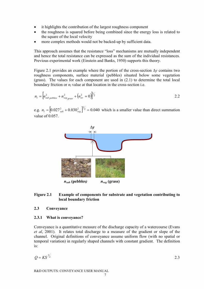
Figure 2.1 provides an example where the portion of the cross-section �y contains tworoughness components, surface material (pebbles) situated below some vegetation(grass). The values for each component are used in (2.1) to determine the total localboundary friction or nl value at that location in the cross-section i.e.
� �� � 21222 0���� irrgrassvegpebblessubl nnnn 2.2
e.g. � � 040.0030.0027.0 2122
��� vegsubln which is a smaller value than direct summationvalue of 0.057.
�y
nsub (pebbles) nveg (grass)
Figure 2.1 Example of components for substrate and vegetation contributing tolocal boundary friction
2.3 Conveyance
2.3.1 What is conveyance?
Conveyance is a quantitative measure of the discharge capacity of a watercourse (Evanset al, 2001). It relates total discharge to a measure of the gradient or slope of thechannel. Original definitions of conveyance assume uniform flow (with no spatial ortemporal variation) in regularly shaped channels with constant gradient. The definitionis:
21
KSQ � 2.3
R&D OUTPUTS: CONVEYANCE USER MANUAL8
where K (m3/s) is the conveyance, Q (m3/s) is the discharge and S is the commonuniform gradient. In idealisation there is no ambiguity about this slope since the watersurface slope, the bed slope and the so-called “energy” or “friction” slope all coincide.For non-uniform geometry, local variations in the section shape influence the watervelocity and therefore the balance between the potential and kinetic energy of the flow,the specific energy, E (m) of the flow is commonly defined by:
gUhE2
2
�� 2.4
where g (m2/s) is the acceleration due to gravity, h (m) is the water surface level of theflow and U (m/s) is the section average velocity. In this case, the slope to be used in thedefinition of conveyance is the magnitude of the gradient, Sf, in the downstream (x-)direction of the specific energy
dxdES f �� 2.5
2.3.2 Why do we need to know about channel conveyance?
The ability of a channel to convey water directly influences the water levels. Resistanceto flow results in smaller velocities and greater depths. Water level prediction isessential for flood management tasks such as flood-forecast warning and flood riskmapping. Flood management practice relies on reliable water level predictions to makeinformed decisions regarding infrastructure design and operation, and more importantly,emergency evacuation planning. Flood levels are also necessary for strategic planningi.e. evaluating and comparing options against criteria, hydrometric users and channelmaintenance i.e. timing, scheduling and prioritisation of dredging and vegetationcutting.
2.3.3 Why is there a new approach for estimating channel conveyance?
Existing methods for estimating conveyance in 1D hydrodynamic models are based onthe Manning equation. This empirically derived equation, first published in 1890, is notbased on rigorous physics and provides unreliable results for sudden changes in area orwetted perimeter with depth, when shape effects are ignored. When applied as aDivided Channel Method i.e. the flow rate calculated separately for the floodplain andmain channel zones and subsequently summed; the lateral shearing and consequentmomentum transfer between the vertical divisions or ‘slices’ is ignored. The Manningequation thus represents all the energy losses though the well-known ‘n’ value (Chow,1959), lumping all the physical flow processes such as shearing and momentum transferinto one ‘catch-all’ parameter, with little understanding and interpretation of theindependent energy “loss” mechanisms.
More recently, there have been advances in the understanding and modelling of thevarious flow processes and the associated energy losses. Research into the exact natureof these mechanisms such as local friction, turbulence due to lateral shearing and thepresence of secondary flows, together with an ever increasing database of observed flowparameters, has provided the facility for testing and validating these new approaches.Significant contributions include those of Chang (1983, 1984), Ervine and Ellis (1987),
R&D OUTPUTS: CONVEYANCE USER MANUAL9
Shiono and Knight (1989), Ackers (1992, 1993), Bousmar and Zech (1999) and Ervineet al (2000). For further details see Evans et al (2001) and DEFRA/EA (2003a).
2.3.4 Do I need to have a strong mathematical background to use the CES?
No. The equations described in this section are all coded within the CES and theyrequire no user manipulation. The section is provided to enable better understandingand description of the conveyance inputs (see Section 3.2) such that the use of the CESis optimised.
2.3.5 What are the different energy loss mechanisms?
The energy “losses” arise through the development of vortex structures on a variety oflength scales. Once vorticity is created, its rotational energy cascades down in lengthscale into increased turbulence intensity, until it dissipates as heat through viscosity.The streamwise translational kinetic energy is thus transferred in part to rotationalkinetic energy, which no longer contributes to the streamwise channel conveyancecapacity. It is possible to identify situations in which the vorticity is increased e.g. thesevortex structures may arise from:
� Boundary friction caused by the resistance due to surface roughness� Turbulence due to lateral shearing in regions with steep velocity gradients e.g.
adjacent to a flow boundary layer; and at the floodplain main channel interface,where the water is flowing faster in the main channel than on the floodplains
� Transverse currents developing in regions of steep velocity gradients. Thesesecondary currents vary with relative depth i.e. they change their orientation as theflow moves from in-bank to out-of-bank flow; and sinuosity i.e. the secondaryflows expand into the bend in a helical-type shape and then gradually dissipatebeyond the bend
� Water moving from the floodplain region into the main channel, which is alsosubject to expansion losses. The velocity i.e. both magnitude and direction of theflow is important here, as high velocity results in a greater shear as the floodplainflow passes over the main channel flow, driving the vorticity structures. Inmeandering channels, this direction may retard or enhance the main streamrotations. Contraction losses may occur as water passes from the main channel intothe floodplain region.
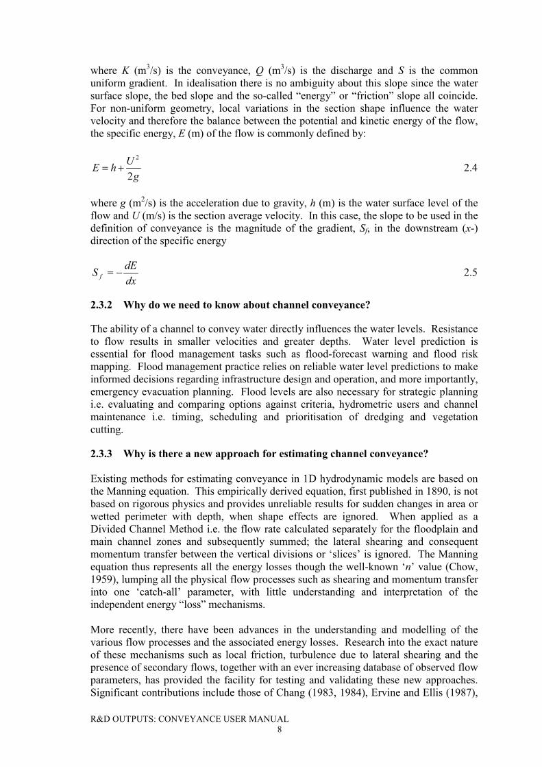
Additional “losses” may arise due to changes in form in non-prismatic channels i.e.channels characterised by rapid changes in channel section over short reaches. Figures2.2-2.4 illustrate these vortex structures and the region where they are likely to occur.
R&D OUTPUTS: CONVEYANCE USER MANUAL10
Lateral shear zones
Secondary flowsBed friction
FloodplainTerraced floodplain Main channel
Figure 2.2 Energy loss mechanisms in a straight compound channel for threedepths of flow
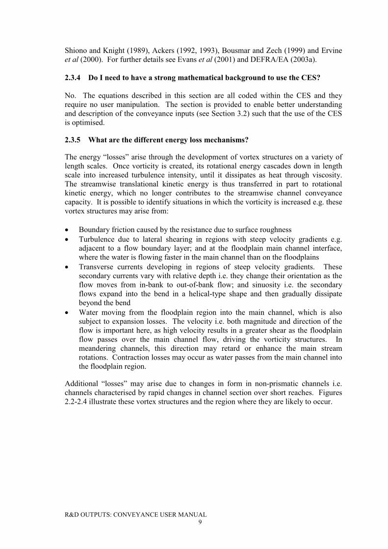
Figure 2.3 Flow mechanisms associated with straight overbank flow in a two-stage channel (Shiono and Knight, 1991)
R&D OUTPUTS: CONVEYANCE USER MANUAL11
Figure 2.4 Flow mechanisms associated with in a two-stage meandering channel(Ervine et al., 2001)
2.3.6 What is the selected approach in the CES for calculating conveyance?
The calculation approach is based on the depth-integrated Reynolds Averaged Navier-Stokes (RANS) equations for flow in the streamwise direction. It extends the originalShiono-Knight Method SKM (Shiono and Knight, 1989) for straight prismatic channels,to include the more recent approach of Ervine et al (2000) for meandering channels.The unit flow rate distribution is determined laterally across the section from(DEFRA/EA, 2003a),
� � � �
���
�
���
�
�
��
�
��
�
�
��
�
���
��
�
�
���
��
�
�
��
Hq
yC
015.00.1
015.0015.1
Hq
yq
8fH
yH8qfgHS
2
uv2
2
o
21
��
��
�
2.6a (I) (II) (III) (IV)
��
���
�
�
��
���
�
���
�
��
�
�
�
��
�
�
���
Hq
yC
Hq
yqfH
yHqf
gHS uvo
2
2
2 21
88�
�2.6b
where:g gravitational acceleration (9.807 m/s2)q streamwise unit flow rate (m2/s)H local depth normal to the channel bed (m)So reach-averaged longitudinal bed slopey lateral distance across the channel (m)� coefficient to account for influence of local bed slope on the bed shear stress
R&D OUTPUTS: CONVEYANCE USER MANUAL12
� reach-averaged sinuosityf local friction factor� dimensionless eddy viscosity� secondary flow parameter – straight channelsCuv meandering coefficient.
Equation 2.6a is applicable for a sinuosity � of 1.0 for inbank flow and 1.0 � � � 1.015for overbank flow. Equation 2.6b is applicable for a sinuosity greater than 1.0 andgreater than 1.015 for inbank and overbank flow respectively. The lateral unit flow ratedistribution can then be integrated to find the total cross-section flow rate Q (m3/s), andhence the total cross-section conveyance K (m3/s), from
21
21
of S
dyq
S
QK ��� 2.7
where the reach-averaged longitudinal friction slope Sf is approximated by the reach-averaged longitudinal bed slope So. The dependence on four experimentally determinedcoefficients, f, �, � and Cuv implies that the method is semi-empirical.
The terms in Equation 2.6a and b represent:
I) An approximation to the variation in hydrostatic pressure along the reach (Sf � So)II) energy losses due to boundary friction effectsIII) turbulence losses due to shearing between the lateral layersIV) turbulence losses due to secondary currents
Term (I), the source or hydrostatic pressure term, is evaluated from the gravitationalacceleration g, the local depth H and the longitudinal bedsope So, as an approximationto Sf.
Term (II), the boundary friction term, and term (I) comprise the primary balance ofmomentum in Equation 2.6a and b. Simplification of these two terms results in thewell-known Darcy-Weisbach friction formula. Term (II) is evaluated from the localdepth H, the local friction factor f and the bed slope coefficient � given by,
� � 2121 yS��� 2.8
where Sy is the transverse bed slope. The lateral distribution of f is based on the local nlvalue provided from the roughness calculation (Section 2.2). This nl value is convertedto an equivalent ks value, through the rough turbulent Colebrook-White Law at areference depth of 1m (based on typical UK river depths), with coefficients suitable foropen channel flow,
���
�
���
�
���
�
�
��
�
�
�
���)03.2(8
1)03.2(8
1027.121027.12
61
ll ngngH
s Hk 2.9
R&D OUTPUTS: CONVEYANCE USER MANUAL13
This ks value is similar to Nikuradse’s sand grain dimension, and in the case ofvegetation, it can be interpreted as an equivalent length scale of the turbulent eddies thatare generated. The reasons for selecting the Colebrook-White equations aredocumented elsewhere DEFRA/EA (2003a).
The method for resolving the lateral distribution of f is dependent on the ks/H ratio. Thereason for this is that the Colebrook-White law is not applicable at high ks/H ratios,since the bracketed term (Equation 2.10) approaches one and the logarithm of one iszero. Further details in DEFRA/EA (2004/5 in preparation). Three categories aredefined:
1. ks/H < 1.66
Here, f is solved from the rough turbulent Colebrook-White Law for natural rivers,
��
���
��
Hk
fs
27.12log03.21 2.10
and from the full Colebrook-White Law (i.e. rough and smooth components) forexperimental flumes,
���
�
���
���
fqHk
fs
409.3
27.12log03.21 � 2.11
2. 1.66 ks/H � 10
Here, f is solved through a Power Law approximation,
Hk
f s
3015.418
� 2.12
3. ks/H > 10
The Power Law approximation (category 2, Equation 2.12) is restricted at amaximum ks/H ratio of 10, i.e.
� � 94.1103015.418
3015.418
���
Hk
f s 2.13
Term (III), the lateral shear term, has a relatively small impact on the total discharge Q.It is evaluated from the local friction f, the local depth H and the dimensionless eddyviscosity �. The lateral distribution of � is given by (Abril, 2002),
� �44.12.12.0 �
��� rmc D�� 2.14
where the main channel value, �mc, is 0.24 (DEFRA/EA, 2003a) and the relative depthDr is defined as the local depth H over the maximum depth. For further detailsregarding the eddy viscosity model see DEFRA/EA (2003a).
R&D OUTPUTS: CONVEYANCE USER MANUAL14
Term (IV), the secondary flow term, changes between Equation 2.6a and b, since thenature of the secondary flow varies with relative depth and planform sinuosity.Equations 2.6a and b are solved for the unit flow rate q rather than the depth-averagedvelocity Ud. This is due to the strong continuity properties of q (Samuels, 1989).Expressing the complete secondary flow term (right hand side of 2.3a and b) in terms ofthe depth-averaged velocities gives,
� �y
UVH d
2.15
where U and V are the streamwise and lateral velocity components respectively, and thesuffix ‘d’ represents depth-averaging. Since the lateral velocity is an additionalunknown, the Conveyance Generator provides a “closure” for this term based on twoprevious approaches: that of Shiono and Knight (1989) for straight prismatic channels,where a secondary flow term � is defined as
� �� �dUVHy
�
�� 2.16
and that of Ervine et al (2000) for meandering channels,
2duvUCUV � 2.17
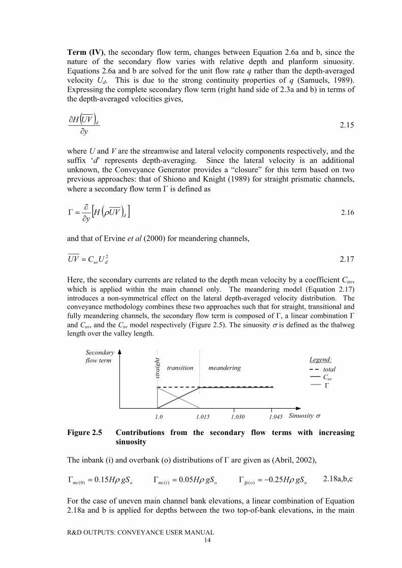
Here, the secondary currents are related to the depth mean velocity by a coefficient Cuv,which is applied within the main channel only. The meandering model (Equation 2.17)introduces a non-symmetrical effect on the lateral depth-averaged velocity distribution. Theconveyance methodology combines these two approaches such that for straight, transitional andfully meandering channels, the secondary flow term is composed of �, a linear combination �and Cuv, and the Cuv model respectively (Figure 2.5). The sinuosity � is defined as the thalweglength over the valley length.
Legend: total Cuv
�
1.0 1.015 1.030 1.045
Secondaryflow term
Sinuosity �
transition meandering
stra
ight
Figure 2.5 Contributions from the secondary flow terms with increasingsinuosity
The inbank (i) and overbank (o) distributions of � are given as (Abril, 2002),
omc gSH�15.0)0( �� oimc gSH�05.0)( �� oofp gSH�25.0)( ��� 2.18a,b,c
For the case of uneven main channel bank elevations, a linear combination of Equation2.18a and b is applied for depths between the two top-of-bank elevations, in the main
R&D OUTPUTS: CONVEYANCE USER MANUAL15
channel region. Equation 2.18a,bandc are only applied in the shear layer i.e. regions ofmixing between the flood plain and main channel. In practice, these typically extendacross the entire main channel region (Samuels, 1988) and over a portion of the floodplain. The flood plain extent is approximated based on the lesser of the main channelwidth and ten times the bankfull depth. For straight channels Cuv = 0. For inbank flowin channels of sinuosity greater than 1.0, Cuv is given by (DEFRA/EA, 2003a),
5395.38669.73274.4 2��� ��uvC [1.0 < � � 2.5 i.e. 0% < Cuv � 11%] 2.19
For overbank flow in channels of sinuosity between 1.0 and 1.015 the secondary flowterm is a linear combination of � and Cuv. For overbank flows in channels of sinuositygreater than 1.015 the secondary flow term Cuv is given by (DEFRA/EA, 2003a),
6257.61659.7 �� �uvC [1.015 < � � 2.500 i.e. 0.6% < Cuv � 11%] 2.20
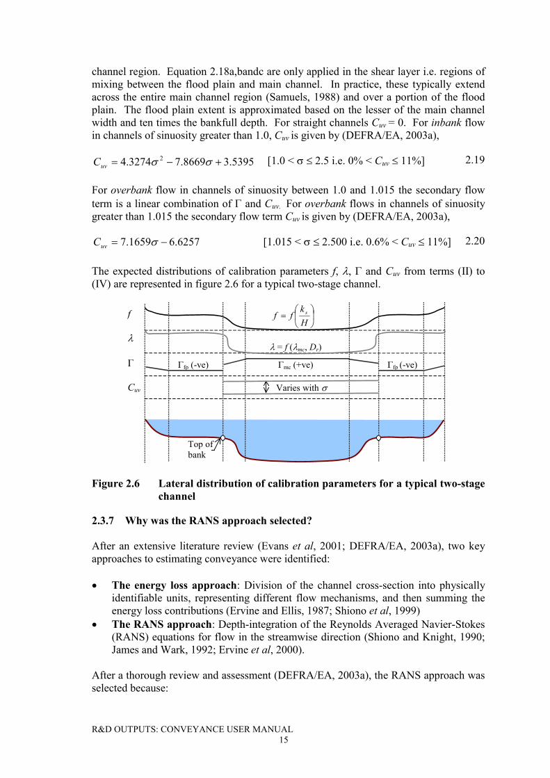
The expected distributions of calibration parameters f, �, � and Cuv from terms (II) to(IV) are represented in figure 2.6 for a typical two-stage channel.
f
�
�
Cuv
�fp (-ve) �mc (+ve) �fp (-ve)
� = f (�mc, Dr)
Varies with �
Top ofbank
��
���
��
Hk
ff s
Figure 2.6 Lateral distribution of calibration parameters for a typical two-stagechannel
2.3.7 Why was the RANS approach selected?
After an extensive literature review (Evans et al, 2001; DEFRA/EA, 2003a), two keyapproaches to estimating conveyance were identified:
� The energy loss approach: Division of the channel cross-section into physicallyidentifiable units, representing different flow mechanisms, and then summing theenergy loss contributions (Ervine and Ellis, 1987; Shiono et al, 1999)
� The RANS approach: Depth-integration of the Reynolds Averaged Navier-Stokes(RANS) equations for flow in the streamwise direction (Shiono and Knight, 1990;James and Wark, 1992; Ervine et al, 2000).
After a thorough review and assessment (DEFRA/EA, 2003a), the RANS approach wasselected because:

R&D OUTPUTS: CONVEYANCE USER MANUAL16
� The RANS approach has a sound physical basis as it is derived from the originalNavier-Stokes equations for fluid flow
� This approach incorporates most of the energy losses outlined in Section 2.3.5. Itincludes boundary friction, lateral shearing and momentum exchange i.e. secondaryflows and expansion / contraction of flow between the main channel andfloodplains. However, form losses are not considered. These can be represented ina one-dimensional hydrodynamic model through discrete energy “losses” e.g. theBernoulli loss unit in ISIS
� The energy loss hierarchy is considered. The lateral distributions of f, � and � varywith depth of flow, and the meandering coefficient Cuv varies with both depth offlow and sinuosity. The result is that the contributions of the different energy lossterms are weighted according to when the relevant loss mechanism is likely tooccur
� Despite having four calibration parameters, f, �, � and Cuv, there are existingmodels that can be adapted to represent the lateral distributions of these terms
� The method can be applied to any river cross-section or planform geometry,including multi-thread meandering two-stage channels. Although an analytical ornumerical solution is required, the implementation is feasible within computercode, without requiring detailed knowledge by the user
� The method allows for changes in local roughness values across the section,enabling representation of localised bed features such as trees, boulders, artificiallining etc.
� The method is applied within a cross-section framework and is thus readilyinterpreted for use within existing 1D hydrodynamic modelling software
� The primary output is the conveyance and flow rate for a given water level. Inaddition, the lateral distribution of the unit flow rate, depth-averaged velocity, bedshear stress and shear velocity is provided. The velocity and bed shear stresses areuseful for vegetation maintenance and sediment transport respectively
� The method has been widely tested against both experimental and real riverobservations, with encouraging results.
The Project Expert Advisory Panel reviewed and approved the scientific basis andapplication of this method.
2.3.8 What are the limitations of this method?
� The conveyance equations are based on the depth-integration of the RANS equationfor flow in the streamwise direction. These equations are inappropriate at highsinuosities, where the main channel velocity vector changes direction abovebankfull depth, such that it is aligned with the mean floodplain direction. The useof depth-averaging is inappropriate in this instance
� Energy losses due to form change are not considered i.e. rapid changes in cross-section between consecutive river sections. In 1D-river models, these losses can berepresented through discrete energy “losses” e.g. the Bernoulli loss unit in ISIS
� There are four calibration parameters, f, �, � and Cuv, which may providedifficulties. E.g. Which parameter is not performing adequately? Which parametershould be altered to achieve calibration? Are the parameters mutually independent?Are the parameters accurately depicting the energy loss mechanisms for which theyare prescribed?
R&D OUTPUTS: CONVEYANCE USER MANUAL17
� The method will take longer computationally than the previous ‘Manning’equation, as an iterative solution is required for each depth of flow. The solution ofEquation 2.6a and b has been designed to converge nearly quadratically, thusreducing the number of iterations to less than 7
� The method is difficult for the ‘casual’ user to understand in detail.
2.3.9 How are the RANS equations solved?
Equations 2.3a and b are non-linear, elliptic, second order partial differential equations.These are approximated numerically, using linear finite elements; a method well suitedto the solution of elliptic equations. The cross-sectional area of flow represents thesolution domain, which is discretised laterally into a number of elements, and thevariable q is replaced with piecewise linear approximations. The solution to theresulting system of discrete equations is generated through an iterative procedure,linearised in the correction term �qn, to update unit flow rate qn+1
from the known qn
value from the previous iteration. The fixed boundary condition, q = 0, is prescribed atthe boundary nodes at the edges of the flow domain. The iteration procedure isdesigned to converge nearly quadratically. For further details regarding the numericalscheme, see DEFRA/EA (2003a).
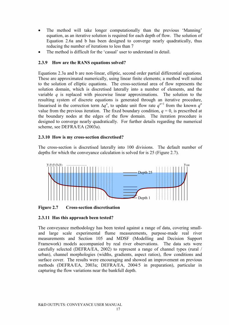
2.3.10 How is my cross-section discretised?
The cross-section is discretised laterally into 100 divisions. The default number ofdepths for which the conveyance calculation is solved for is 25 (Figure 2.7).
y1y2y3y4y5 ……………. y100
Depth 25
Depth 1
Figure 2.7 Cross-section discretisation
2.3.11 Has this approach been tested?
The conveyance methodology has been tested against a range of data, covering small-and large scale experimental flume measurements, purpose-made real rivermeasurements and Section 105 and MDSF (Modelling and Decision SupportFramework) models accompanied by real river observations. The data sets werecarefully selected (DEFRA/EA, 2002) to represent a range of channel types (rural /urban), channel morphologies (widths, gradients, aspect ratios), flow conditions andsurface cover. The results were encouraging and showed an improvement on previousmethods (DEFRA/EA, 2003a; DEFRA/EA, 2004/5 in preparation), particular incapturing the flow variations near the bankfull depth.
R&D OUTPUTS: CONVEYANCE USER MANUAL18
2.4 Uncertainty
2.4.1 What is uncertainty?
One definition of uncertainty is as follows:
“Uncertainty is a general concept that reflects our lack of sureness about something orsomeone, ranging from just short of complete sureness to an almost complete lack ofconviction about an outcome”
Uncertainty arises principally from lack of knowledge or of ability to measure or tocalculate and gives rise to potential differences between assessment of some factor andits “true” value. Understanding this uncertainty within our predictions and decisions isat the heart of understanding risk. Within uncertainty we are able to identify:
� knowledge uncertainty arising from our lack of knowledge of the behaviour of thephysical world
� natural variability arising from the inherent variability of the real world� decision uncertainty which reflects the complexity of our social and organisational
values and objectives.
However, this classification is not rigid or unique. For example, uncertainty on weatheror climate will be taken as “natural variability” within flood risk management but as“knowledge uncertainty” in the context of climate simulation. It is helpful also toconsider the differences between accuracy, error and uncertainty. Accuracy and errordiffer from uncertainty as defined above but limitations in accuracy or the possibility forhuman error will contribute to the overall uncertainty.
� Accuracy has two facets. It deals with the precision to which measurement orcalculation is carried out (i.e. the maximum deviation of the measurement orcalculation from the “true” amount) and with the number of digits of precisionwhich are carried through a calculation (whether or not these are meaningful).Potentially, accuracy can be improved by better technology.
� Errors are mistaken calculations or measurements with quantifiable andpredictable differences from the actual value.
2.4.2 Why do I need to account for uncertainty?
Consideration of uncertainty within the decision process attempts to provide bounds toour lack of sureness and thereby provides the decision-maker with a better context inwhich to take a decision. Through investigation of the sources of uncertainty, this typeof analysis enables the engineer or decision-maker to identify the uncertainties that mostinfluence the final outcome and focus resources efficiently. By understanding thesources and importance of uncertainty within our decisions, we should be able to makebetter and more informed choices.
The effects of uncertainty in the estimation of conveyance differ with the variousprocess undertaken by the Agency. The potential consequences of uncertainty andtypical current methods of mitigation for the uncertainty in conveyance are listed inTable 2.1 below. The sensitivity of project decisions to uncertainty in conveyanceestimation needs to be established as strategic decisions made early in the project life

R&D OUTPUTS: CONVEYANCE USER MANUAL19
cycle can have far reaching consequences but it is at this early stage that uncertainties ininformation and data are greatest.
Table 2.1 Potential consequences of uncertainty in flood conveyance
AgencyActivity Catchment-wide consequence of uncertainty Typical mitigation
strategyStrategicPlanning
Inadequate framework for long-term view of flood risk at acatchment scale, leading to sub-optimal or inadequatestrategies and solutions. Potential unexpected long-termincrease in flood impacts on people and properties.
Undertake sensitivitytesting to bound theexpected results
Flood defencedesign
Under capacity of defences leading to potential failure belowthe design standard or over capacity potentially leading tomorphological problems or lower economic return thanplanned; over estimation of capacity of defences leading tolack of implementation of schemes due to excessive cost.
Undertake sensitivityanalyses and add afreeboard to allow forunder capacity
Maintenance Inadequate or excessive maintenance activities, possiblyunnecessary disruption to aquatic and riparian habitats orinsufficient capacity of the watercourse leading to increasedflood risk.
Maintain to a definedprogramme
Real timeforecasting
Inaccuracies in the threshold trigger levels, under- (over-)estimation of lead times, inexact inundation extent, andincorrect retention times of floods.
Implement real-timeupdating procedures
Hydrometry -Rating curveextension
Incorrect discharges with potentially large errors, influencesflood forecasting and statistical estimation of flood flows fordesign, impacts upon cost-benefit assessment and decisionsto promote flood defence schemes.
Undertake sensitivityanalyses
Regulation Indicative Flood Mapping (IFM) in error – inadequate toolfor planning and information on possible flood risk,inadequate (or over necessary) development control, loss ofprofessional and public confidence in the Agency’s technicalabilities.
Give “health warnings”on use of IFM
There is a close relationship between uncertainty and risk in that the greater theuncertainty the greater the potential of the project or maintenance activity of notachieving its objective. This is linked to the confidence on the performance of thescheme or process to meet its intended objectives. Thus, optimisation of performanceand the confidence with which performance can be achieved is linked inexorably withunderstanding and controlling uncertainty.
2.4.3 What factors contribute to the uncertainty in conveyance?
The uncertainties in conveyance estimation are principally due to natural variability andknowledge uncertainty. Two contributions are normally recognised in knowledge uncertainty;these are:
� Process model uncertainty in any deterministic approach used in the assessment� Statistical uncertainty arising from the selection and fitting of statistical
distributions and parameters from data within the assessment.
In the Conveyance Estimation System no use is made of statistical modelling and soissues of statistical uncertainty do not arise. However, in the overall estimation of floodrisk there will be an important component of statistical uncertainty arising from anyhydrological estimation procedures for flood flow.
R&D OUTPUTS: CONVEYANCE USER MANUAL20
There are several important components of process model uncertainty in the estimationof river and flood plain conveyance.
� process model uncertainty arising from the selection and approximation ofphysical processes and from parameterisation made in the definition ofconveyance
� representation of topography through the density of discrete survey points andinterpolation rules between them, i.e. the difference between the profile of the riverand of the physical features on the flood plain as represented in the calculations andthe river in “real” life
� uncertainty related to data accuracy from the limitations of the survey methodsused
� uncertainties arising from parameter estimation – particularly the experience andexpertise of the modellers who set up and calibrate computational models of riverflows
� uncertainties from the model calculation methods, approximations and rules; theseare the domain of traditional numerical analysis.
The contributions to uncertainty from natural variability include:
� seasonality of plant growth from variation in temperature, light and nutrients (andhence resistance of vegetation in channels)
� “memory” in the system e.g. arising from vegetation or river bed conditions beingdifferent after a high flow from the conditions before the event or through episodicinput of sediments into the river system washed off the land surface
� secondary influences of temperature on water viscosity and hence Reynolds’number and flow and sediment transport capacity of channels.
2.4.4 What approaches for estimating uncertainty were considered?
There are several approaches to the assessment of uncertainty, depending upon the typeand extent of information available and the type of decision to be made.
The Italian Flag concept
This involves a decision process where the results are given a green light for reliableresults, a white light for some uncertainty or a red light for poor results. Each parameteris given a colour rating and the overall colour is then assessed. This method is limitedas it is based on subjective decisions, cannot be quantified and within the white area, thelevel of uncertainty cannot be determined, e.g. closer to green or red.
Scenario Assessment and Climate Impact Analysis
The Intergovernmental Panel on Climate Change (IPCC) is overseeing the internationalresearch effort on assessment of potential climate change, its environmental and socialimpacts and policy responses. This is an area where complex interactions abound andthere is significant uncertainty inherent in the “predictions”. The IPCC has issuedguidance on the treatment and interpretation of uncertainty in the context of climatemodelling, impact analysis and consequent decisions (IPCC, 2001). Climate changeimpact analysis is conducted in terms of “scenarios” which set as inputs atmospheric
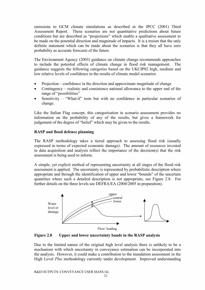
R&D OUTPUTS: CONVEYANCE USER MANUAL21
emissions to GCM climate simulations as described in the IPCC (2001) ThirdAssessment Report. These scenarios are not quantitative predictions about futureconditions but are described as “projections” which enable a qualitative assessment tobe made on the potential direction and magnitude of impacts. It is a truism that the onlydefinite statement which can be made about the scenarios is that they all have zeroprobability as accurate forecasts of the future.
The Environment Agency (2003) guidance on climate change recommends approachesto include the potential effects of climate change in flood risk management. Theguidance suggests the following categories based on the UKCIP02 high, medium andlow relative levels of confidence in the results of climate model scenarios
� Projection – confidence in the direction and approximate magnitude of change� Contingency – realistic and consistence national allowance to the upper end of the
range of “possibilities”� Sensitivity – “What-if” tests but with no confidence in particular scenarios of
change.
Like the Italian Flag concept, this categorisation in scenario assessment provides noinformation on the probability of any of the results, but gives a framework forjudgement of the degree of “belief” which may be given to the results.
RASP and flood defence planning
The RASP methodology takes a tiered approach to assessing flood risk (usuallyexpressed in terms of expected economic damage). The amount of resources investedin data acquisition and analysis reflect the importance of the decision(s) that the riskassessment is being used to inform.
A simple, yet explicit method of representing uncertainty at all stages of the flood riskassessment is applied. The uncertainty is represented by probabilistic description whereappropriate and through the identification of upper and lower “bounds” of the uncertainquantities where such a detailed description is not appropriate, see Figure 2.8. Forfurther details on the three levels see DEFRA/EA (2004/2005 in preparation).
uppercentral lower
Waterlevel ordamage
Flow/ loading
Figure 2.8 Upper and lower uncertainty bands in the RASP analysis
Due to the limited nature of the original high level analysis there is unlikely to be amechanism with which uncertainty in conveyance estimation can be incorporated intothe analysis. However, it could make a contribution to the inundation assessment in theHigh Level Plus methodology currently under development. Improved understanding
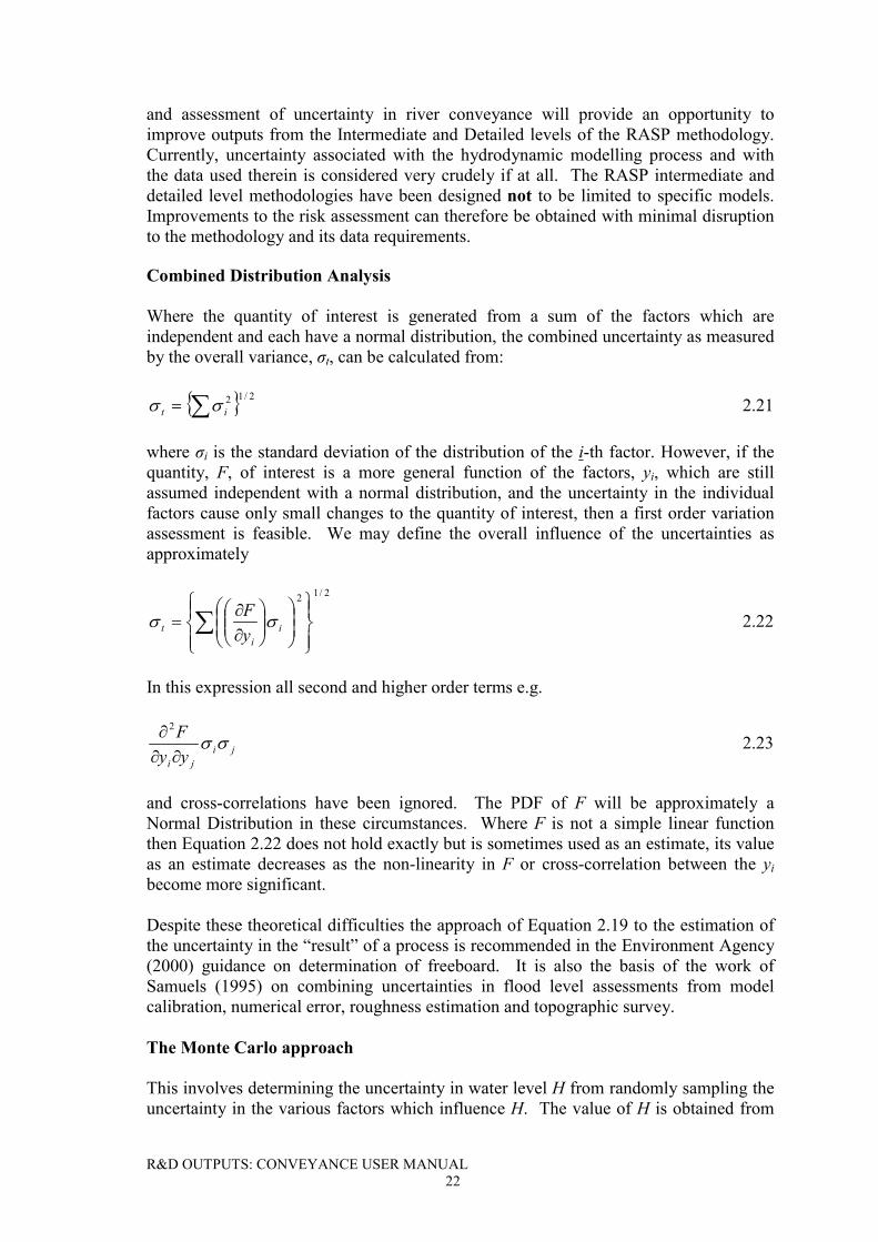
R&D OUTPUTS: CONVEYANCE USER MANUAL22
and assessment of uncertainty in river conveyance will provide an opportunity toimprove outputs from the Intermediate and Detailed levels of the RASP methodology.Currently, uncertainty associated with the hydrodynamic modelling process and withthe data used therein is considered very crudely if at all. The RASP intermediate anddetailed level methodologies have been designed not to be limited to specific models.Improvements to the risk assessment can therefore be obtained with minimal disruptionto the methodology and its data requirements.
Combined Distribution Analysis
Where the quantity of interest is generated from a sum of the factors which areindependent and each have a normal distribution, the combined uncertainty as measuredby the overall variance, σt, can be calculated from:
� � 2/12�� it �� 2.21
where σi is the standard deviation of the distribution of the i-th factor. However, if thequantity, F, of interest is a more general function of the factors, yi, which are stillassumed independent with a normal distribution, and the uncertainty in the individualfactors cause only small changes to the quantity of interest, then a first order variationassessment is feasible. We may define the overall influence of the uncertainties asapproximately
2/12
��
���
��
���
��
��
�
��
���
�
�� � i
it y
F�� 2.22
In this expression all second and higher order terms e.g.
jiji yy
F��
��
�2
2.23
and cross-correlations have been ignored. The PDF of F will be approximately aNormal Distribution in these circumstances. Where F is not a simple linear functionthen Equation 2.22 does not hold exactly but is sometimes used as an estimate, its valueas an estimate decreases as the non-linearity in F or cross-correlation between the yibecome more significant.
Despite these theoretical difficulties the approach of Equation 2.19 to the estimation ofthe uncertainty in the “result” of a process is recommended in the Environment Agency(2000) guidance on determination of freeboard. It is also the basis of the work ofSamuels (1995) on combining uncertainties in flood level assessments from modelcalibration, numerical error, roughness estimation and topographic survey.
The Monte Carlo approach
This involves determining the uncertainty in water level H from randomly sampling theuncertainty in the various factors which influence H. The value of H is obtained from
R&D OUTPUTS: CONVEYANCE USER MANUAL23
taking sample values of each of the parameters that influence it e.g. channel and floodplain Manning’s n (or each component to the unit Manning’s n), bed level, yi, at eachpoint across the section (if sediment processes are important) etc. The variability ofeach parameter is described through an associated probability distribution function(PDF) and possibly with cross-correlation relationships. The output H is obtained for alarge number (potentially thousands) of randomly selected samples from eachdistribution using cross-correlation to obtain conditional probabilities if the factors arenot independent. The frequency distribution for H is then compiled from therealisations obtained and possible a new PDF fitted. See Figure 2.9 below.
,...),( ifc ynnFH �
PDF for nc PDF for nf PDF for yi
Combine many samples togenerate output PDF
Random sampleof each PDF
PDF for H
Figure 2.9 The Monte Carlo approach
The advantage of this method is that an uncertainty distribution is obtained based on thesum effect of the individual PDFs and the method can be extended to add in theinfluence of more factors, such as the variability in the flood flows from hydrologicalassessment. The method is rigorous if the PDF is known for each of the inputparameters, and can be used to estimate the variability of the results from assumptionsabout the input PDFs where these are not known.
However, the approach is computationally intensive where there are many parameters totest and if the method is used to assess the variability of the result to assumptions onunknown distribution. If the approach is set within a larger analysis (such as acomputational river model and incorporating hydrological PDFs) then the method mynot be feasible for practical use.
2.4.5 How is uncertainty represented in the CES?
A key decision in developing advice and estimates of uncertainty was on how theinformation should be presented. Several approaches are possible as described abovebut some require considerable additional information and analysis to generate theresults. Thus an appropriate starting point was to consider the users of the CES andhow they might incorporate information on uncertainty into their decisions. This led tosome requirements of the method in practice, it should:
R&D OUTPUTS: CONVEYANCE USER MANUAL24
� express uncertainty in water level� link to and inform other Environment Agency - Defra risk approaches� be understandable to the user to facilitate better, more informed decisions in the
situations they are responsible for� be as simple as possible in presentation� not require significant computational resources� ideally not require any additional input data� be credible by being based on existing scientific methods for uncertainty where
possible.
The potential direct and indirect users of the CES information have different needs forinformation on uncertainty in the decisions and plans they need to make. The projectteam’s review of needs of different users identified the potential use, importance andform of presentation of information on uncertainty as shown in Table 2.2 below.
Table 2.2 Summary of Uncertainty users and their needs
User community Use of uncertainty Importance Suitable presentation ofuncertainty
Strategic Planning Evaluating / comparing optionsagainst criteria such aseffectiveness, efficiency,robustness, performance
High Upper and lower estimates
Scheme Design Change in water level for givenflow rate (moving towardsprobabilistic optimisation fordescribing uncertainty)
Medium to high Upper and lower estimatesPotentially probabilisticinformation for a full risk-based design appraisal of amajor scheme
Maintenance Timing, scheduling andprioritisation of vegetationcutting and dredging
Low to medium Upper and lower estimates ornothing
Flood Forecastingand Warning
Minimise false alarm andmissed opportunitiesAid operational decisions
Low in currentpractices
Possibly an upper estimate offlood level (and earlyestimate of arrival time)
Hydrometry Flow rate for a given depth(influences other stakeholders)
Medium (butshould be high)
Upper/lower estimatesProbabilistic
Regulation,insurance
Water levels, flood outlines,indicative flood risk mapping,
High Upper/lower estimates
There is a need for quantitative information on uncertainty so that the “Italian Flag”representation cannot be used in isolation. The approach finally adopted to respond tothe user requirements combined elements of the other approaches described in Section2.4.4 above. In terms of presenting quantitative information on uncertainty theimportant choices are whether to:
� recommend the use of Monte-Carlo testing based� assign probabilities to the information given on uncertainty.
It was decided not to recommend either of these because:
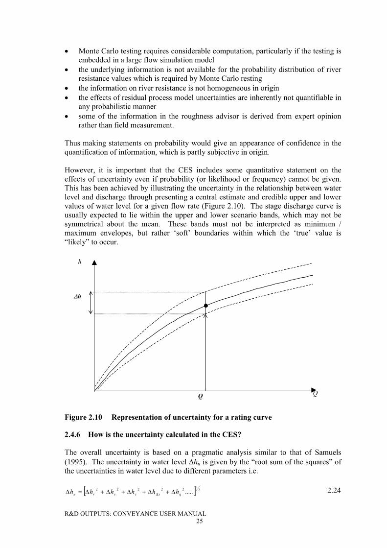
R&D OUTPUTS: CONVEYANCE USER MANUAL25
� Monte Carlo testing requires considerable computation, particularly if the testing isembedded in a large flow simulation model
� the underlying information is not available for the probability distribution of riverresistance values which is required by Monte Carlo resting
� the information on river resistance is not homogeneous in origin� the effects of residual process model uncertainties are inherently not quantifiable in
any probabilistic manner� some of the information in the roughness advisor is derived from expert opinion
rather than field measurement.
Thus making statements on probability would give an appearance of confidence in thequantification of information, which is partly subjective in origin.
However, it is important that the CES includes some quantitative statement on theeffects of uncertainty even if probability (or likelihood or frequency) cannot be given.This has been achieved by illustrating the uncertainty in the relationship between waterlevel and discharge through presenting a central estimate and credible upper and lowervalues of water level for a given flow rate (Figure 2.10). The stage discharge curve isusually expected to lie within the upper and lower scenario bands, which may not besymmetrical about the mean. These bands must not be interpreted as minimum /maximum envelopes, but rather ‘soft’ boundaries within which the ‘true’ value is“likely” to occur.
�h
h
Q Q
Figure 2.10 Representation of uncertainty for a rating curve
2.4.6 How is the uncertainty calculated in the CES?
The overall uncertainty is based on a pragmatic analysis similar to that of Samuels(1995). The uncertainty in water level �hu is given by the “root sum of the squares” ofthe uncertainties in water level due to different parameters i.e.
� � 2122222 .....qxcsru hhhhhh �����������
� 2.24
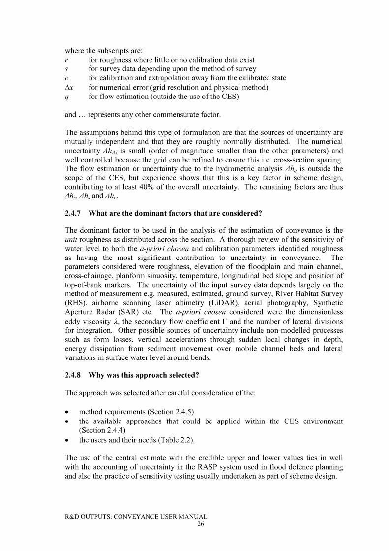
R&D OUTPUTS: CONVEYANCE USER MANUAL26
where the subscripts are:r for roughness where little or no calibration data exists for survey data depending upon the method of surveyc for calibration and extrapolation away from the calibrated state�x for numerical error (grid resolution and physical method)q for flow estimation (outside the use of the CES)
and … represents any other commensurate factor.
The assumptions behind this type of formulation are that the sources of uncertainty aremutually independent and that they are roughly normally distributed. The numericaluncertainty ∆h∆x is small (order of magnitude smaller than the other parameters) andwell controlled because the grid can be refined to ensure this i.e. cross-section spacing.The flow estimation or uncertainty due to the hydrometric analysis ∆hq is outside thescope of the CES, but experience shows that this is a key factor in scheme design,contributing to at least 40% of the overall uncertainty. The remaining factors are thus∆hr, ∆hs and ∆hc.
2.4.7 What are the dominant factors that are considered?
The dominant factor to be used in the analysis of the estimation of conveyance is theunit roughness as distributed across the section. A thorough review of the sensitivity ofwater level to both the a-priori chosen and calibration parameters identified roughnessas having the most significant contribution to uncertainty in conveyance. Theparameters considered were roughness, elevation of the floodplain and main channel,cross-chainage, planform sinuosity, temperature, longitudinal bed slope and position oftop-of-bank markers. The uncertainty of the input survey data depends largely on themethod of measurement e.g. measured, estimated, ground survey, River Habitat Survey(RHS), airborne scanning laser altimetry (LiDAR), aerial photography, SyntheticAperture Radar (SAR) etc. The a-priori chosen considered were the dimensionlesseddy viscosity �, the secondary flow coefficient � and the number of lateral divisionsfor integration. Other possible sources of uncertainty include non-modelled processessuch as form losses, vertical accelerations through sudden local changes in depth,energy dissipation from sediment movement over mobile channel beds and lateralvariations in surface water level around bends.
2.4.8 Why was this approach selected?
The approach was selected after careful consideration of the:
� method requirements (Section 2.4.5)� the available approaches that could be applied within the CES environment
(Section 2.4.4)� the users and their needs (Table 2.2).
The use of the central estimate with the credible upper and lower values ties in wellwith the accounting of uncertainty in the RASP system used in flood defence planningand also the practice of sensitivity testing usually undertaken as part of scheme design.
R&D OUTPUTS: CONVEYANCE USER MANUAL27
The concentration of the scenarios on the influence of uncertainty in river roughness(Section 2.4.7) is justified in terms of the sensitivity analysis undertaken in the testingphase of the CES research (See DEFRA/EA, 2004/2005 in preparation).
2.4.9 What is the effect of calibration?
Calibration of the flow resistance alters the uncertainty in the estimation of conveyance.Calibration data for flow resistance should supersede the generic, non-site specificinformation in the Roughness Advisor. Calibration may result in a different value forthe central estimate of water level for the calibration flow rate and there is no guaranteethat a single roughness value will achieve a perfect calibration for water levels and flowrates observed on different occasions (due to natural variability). However, once themodel has been calibrated, ∆hr and ∆hs are likely to decrease, narrowing the range ofuncertainty, see Figure 2.11 but the exact PDFs for the calibrated and uncalibrated caseswill be difficult to determine.
E(h)calibrated E(h)uncalibrated
Reduced uncertainty due tocalibration
Water Level, h
Calibrated
Uncalibrated
Figure 2.11 Effect of calibration
2.5 Backwater
2.5.1 What is a backwater profile?
A backwater profile is present where there is a disturbance to the normal depth of flow.The effect of the disturbance is felt upstream and the backwater length is the distanceupstream before normal depth is re-established. Typically backwater profiles occurupstream of structures such as reservoirs, weirs and bridges.
2.5.2 Why do I need to know about backwater effects?
� For determining the upstream influence of works in a river channel. The backwaterlength may extend far upstream, potentially causing inundation in areas farupstream of the study reach. Table 2.3 provides some typical UK backwaterlengths
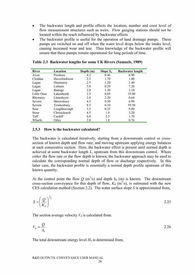
R&D OUTPUTS: CONVEYANCE USER MANUAL28
� The backwater length and profile effects the location, number and crest level offlow measurement structures such as weirs. Flow gauging stations should not belocated within the reach influenced by backwater effects
� The backwater profile is useful for the operation of land drainage pumps. Thesepumps are switched on and off when the water level drops below the intake level,causing increased wear and tear. Thus knowledge of the backwater profile willensure that these pumps remain operational for long periods of time.
Table 2.3 Backwater lengths for some UK Rivers (Samuels, 1989)
River Location Depth (m) Slope So Backwater lengthAvon Pershore 4.2 0.46 6.90Cleddau Haverfordwest 2.5 1.70 1.00Lagan Dunmurry 2.5 1.20 1.40Lagan Lisburn 3.0 0.29 7.20Lagan Banoge 2.0 1.30 1.10Little Ouse Lakenheath 2.5 0.05 35.00Rhymney Llanedeyrn 2.0 2.20 0.64Severn Shrewsbury 4.5 0.50 6.90Severn Tewkesbury 8.5 0.10 59.50Soar Loughborough 3.5 0.25 9.80Stour Christchurch 4.5 1.0 3.20Taff Cardiff 6.0 2.5 1.70Wharfe Otley 2.0 1.8 0.76
2.5.3 How is the backwater calculated?
The backwater is calculated iteratively, starting from a downstream control or cross-section of known depth and flow rate; and moving upstream applying energy balancesat each consecutive section. Here, the backwater effect is present until normal depth isachieved at some backwater length L, upstream from this downstream control. Whereeither the flow rate or the flow depth is known, the backwater approach may be used tocalculate the corresponding normal depth of flow or discharge respectively. In thislatter case, the backwater profile is essentially a normal depth profile upstream of thisknown quantity.
At the control point the flow Q (m3/s) and depth h0 (m) is known. The downstreamcross-section conveyance for this depth of flow, K0 (m3/s), is estimated with the newCES calculation method (Section 2.2). The water surface slope S is approximated from,
21
0���
����
��
KQS 2.25
The section average velocity V0 is calculated from.
00 A
QV � 2.26
The total downstream energy level H0 is determined from,
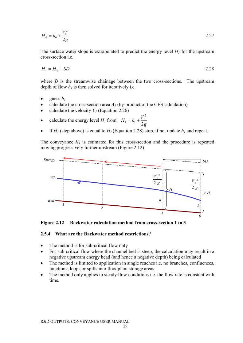
R&D OUTPUTS: CONVEYANCE USER MANUAL29
gV
hH2
20
00 �� 2.27
The surface water slope is extrapolated to predict the energy level H1 for the upstreamcross-section i.e.
SDHH �� 01 2.28
where D is the streamwise chainage between the two cross-sections. The upstreamdepth of flow h1 is then solved for iteratively i.e.
� guess h1� calculate the cross-section area A1 (by-product of the CES calculation)� calculate the velocity V1 (Equation 2.26)
� calculate the energy level H1 from g
VhH2
21
11 ��
� if H1 (step above) is equal to H1 (Equation 2.28) stop, if not update h1 and repeat.
The conveyance K1 is estimated for this cross-section and the procedure is repeatedmoving progressively further upstream (Figure 2.12).
Ho
H1
01
23 h
gV o
2
2g
V2
21
h
SD
Bed
WL
Energy
Figure 2.12 Backwater calculation method from cross-section 1 to 3
2.5.4 What are the Backwater method restrictions?
� The method is for sub-critical flow only� For sub-critical flow where the channel bed is steep, the calculation may result in a
negative upstream energy head (and hence a negative depth) being calculated� The method is limited to application in single reaches i.e. no branches, confluences,
junctions, loops or spills into floodplain storage areas� The method only applies to steady flow conditions i.e. the flow rate is constant with
time.

R&D OUTPUTS: CONVEYANCE USER MANUAL30
R&D OUTPUTS: CONVEYANCE USER MANUAL31
3. USING THE CES
This section provides modelling advice for the three core components of the CES: theRoughness Advisor, the Conveyance Generator and the Uncertainty Estimator, as wellas the use of advanced options, advice on model calibration and interpretation ofconveyance curves with unusual characteristics.
3.1 Roughness advisor
3.1.1 What is the Roughness Advisor?
The Roughness Advisor is a component of the CES software, which provides roughnessadvice based on channel descriptions, photographs and grid references. The roughnessvalues are based on the findings of an extensive literature review (DEFRA/EA, 2003b).Information is included on surface materials [e.g. natural: bedrock, cobbles, gravel,sand, silt, clay, peat, earth, firm soil and manmade: sheet piling, stone block, hazelhurdles, gabion, concrete, rip-rap, wood piling etc], vegetation morpho-types,vegetation categories due to human intervention [e.g. grass, hedges, trees, shrubs andcrops: wheat, sorghum, sunflower, corn, cotton etc] and irregularities [urban trash,groynes, pools and riffles, obstructions]. For the vegetation, the expected seasonalvariations are available.
3.1.2 What will the Roughness Advisor provide?
The Roughness Advisor provides total unit roughness values, comprised of up to threecomponent roughness values: surface material, vegetation and irregularities (Sections2.1.6 and 2.1.7). Mid, upper and lower total unit roughness values are provided, basedon the mid, upper and lower unit roughness values for each component. This range ofroughness values reflects what is expected within these natural systems. Each total unitroughness value is assigned to a zone (Section 3.1.4), since cross-sections passingthrough plan areas or ‘zones’ with similar roughness characteristics will use the sametotal unit roughness value.
3.1.3 What is a roughness zone type?
Each roughness zone has a type. Three roughness zone types have been establishedwithin the Roughness Advisor: bed, bank and floodplain. These are designed toencourage user awareness of the different roughness components that are typicallyfound in these regions e.g. crops are more likely to occur on the floodplains than on thechannel banks or bed. These zone types have no influence on the calculation processand are purely descriptive.
3.1.4 What is a roughness zone?
A roughness zone is a plan area depicting a region of similar roughness characteristicsi.e. similar total unit roughness values. Figure 3.1 shows a plan view of a meanderingchannel situated in a reach with straight floodplains. The plan area has been dividedinto roughness zones e.g. on the floodplain there are areas with reeds and sand; bushesand coarse sand; crops and grass which each represent a roughness zone. Similarly, themain channel can be divided up into however many sections are required to describe thelocal roughness properties.
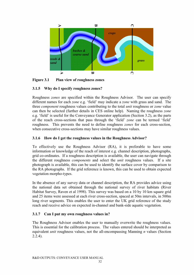
R&D OUTPUTS: CONVEYANCE USER MANUAL32
CBA
CBA
bushes &coarse sand
crops
grassreeds &sand
Figure 3.1 Plan view of roughness zones
3.1.5 Why do I specify roughness zones?
Roughness zones are specified within the Roughness Advisor. The user can specifydifferent names for each zone e.g. ‘field’ may indicate a zone with grass and sand. Thethree component roughness values contributing to the total unit roughness or zone valuecan then be selected (further details in CES online help). Naming the roughness zonee.g. ‘field’ is useful for the Conveyance Generator application (Section 3.2), as the partsof the reach cross-sections that pass through the ‘field’ zone can be termed ‘field’roughness. This prevents the need to define roughness zones for each cross-section,when consecutive cross-sections may have similar roughness values.
3.1.6 How do I get the roughness values in the Roughness Advisor?
To effectively use the Roughness Advisor (RA), it is preferable to have someinformation or knowledge of the reach of interest e.g. channel description, photographs,grid co-ordinates. If a roughness description is available, the user can navigate throughthe different roughness components and select the unit roughness values. If a sitephotograph is available, this can be used to identify the surface cover by comparison tothe RA photographs. If the grid reference is known, this can be used to obtain expectedvegetation morpho-types.
In the absence of any survey data or channel description, the RA provides advice usingthe national data set obtained through the national survey of river habitats (RiverHabitat Survey, Raven et al 1998). This survey was based on a 10 by 10 km square gridand 25 items were assessed at each river cross-section, spaced at 50m intervals, in 500mlong river segments. This enables the user to enter the UK grid reference of the studyreach and receive advice on expected in-channel and bank-side aquatic vegetation.
3.1.7 Can I put my own roughness values in?
The Roughness Advisor enables the user to manually overwrite the roughness values.This is essential for the calibration process. The values entered should be interpreted asequivalent unit roughness values, not the all-encompassing Manning n values (Section2.2.4).

R&D OUTPUTS: CONVEYANCE USER MANUAL33
3.1.8 Are there minimum and maximum allowable unit roughness values?
The CES allows a minimum total unit roughness of 0.0109. This corresponds to anequivalent roughness size ks of 0.1 mm. Roughness values which are smaller than thisminimum value are outside the range of practical application in river engineering.Although the user may overwrite the individual unit roughness values such that thecombined zone value falls below 0.0109, this value will be altered within the CESsoftware to the minimum value of 0.0109.
There is no upper limit on the unit roughness, however the conversion of the total unitor zone roughness nl to the roughness size ks (Section 2.3.6) restricts ks to an upper limitof 12.27m. This large roughness size, which in most instances is greater than the waterdepth, can be interpreted as the size of the horizontal eddies generated from largeobstructions e.g. boulders, tree stumps. This large value is extremely unlikely to bereached in any practical engineering applications.
3.1.9 What are the seasonal variations in vegetation?
The Roughness Advisor provides seasonal variations in the unit roughness for thevegetation morpho-types (where there is available data). This enables the user to enterthe exact date for which they want the roughness predictions, and receive expert adviceon the expected biomass, percentage cover and roughness values for that date.
3.1.10 How are the cutting regimes used?
The Roughness Advisor provides the facility to implement cutting regimes e.g. thepercentage vegetation cutback and the associated date. It will then advise on theexpected post-cutting growth pattern. This enables the user to consider different cuttingregimes (timing, amount) and their effect on the total conveyance.
3.2 Conveyance Generator
3.2.1 How do I describe the cross-section geometry?
The cross-section geometry is described in terms of the offset distance y (m) from theleft bank and elevation z (mAOD). The offset distance should increase from aminimum value on the left bank to a maximum value on the opposite (right) bank. E.g.the cross-sections in Figure 3.2 cannot be solved for within the Conveyance Generator.
The prescribed elevations need not have maximum values at the extreme ends i.e. thechannel banks. The Conveyance Generator introduces two additional co-ordinates ateach end, with identical offsets to the extreme / channel edge values and elevations setat 1.5 times the maximum elevation relative to the bed level within the cross-section(Figure 3.3).
For the case of cross-sections with rapidly rising banks on the floodplain edges, wherethe maximum bank elevation is far greater than the expected maximum flood level, thismaximum calculation depth may be unreasonably high. This will result in theconveyance being calculated at high depths, beyond the range of expected water levels,and fewer conveyance calculation depths in the area of interest e.g. main channel / lowoverbank flows. There are three available for improved predictions:
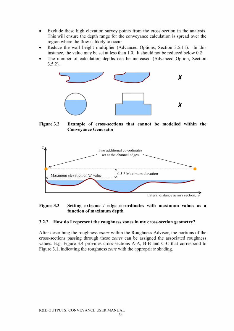
R&D OUTPUTS: CONVEYANCE USER MANUAL34
� Exclude these high elevation survey points from the cross-section in the analysis.This will ensure the depth range for the conveyance calculation is spread over theregion where the flow is likely to occur
� Reduce the wall height multiplier (Advanced Options, Section 3.5.11). In thisinstance, the value may be set at less than 1.0. It should not be reduced below 0.2
� The number of calculation depths can be increased (Advanced Option, Section3.5.2).
�
�
Figure 3.2 Example of cross-sections that cannot be modelled within theConveyance Generator
z
Lateral distance across section, y
Maximum elevation or ‘z’ value 0.5 * Maximum elevation
Two additional co-ordinatesset at the channel edges
Figure 3.3 Setting extreme / edge co-ordinates with maximum values as afunction of maximum depth
3.2.2 How do I represent the roughness zones in my cross-section geometry?
After describing the roughness zones within the Roughness Advisor, the portions of thecross-sections passing through these zones can be assigned the associated roughnessvalues. E.g. Figure 3.4 provides cross-sections A-A, B-B and C-C that correspond toFigure 3.1, indicating the roughness zone with the appropriate shading.
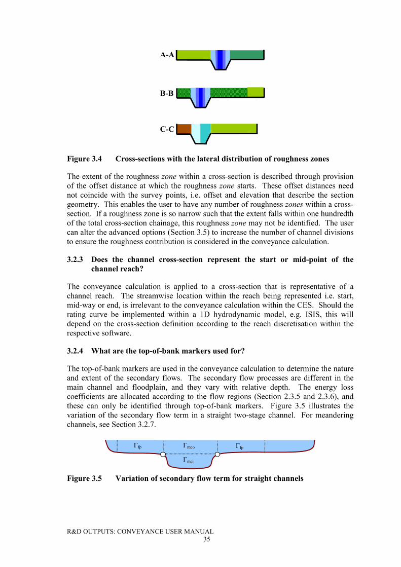
R&D OUTPUTS: CONVEYANCE USER MANUAL35
A-A
B-B
C-C
Figure 3.4 Cross-sections with the lateral distribution of roughness zones
The extent of the roughness zone within a cross-section is described through provisionof the offset distance at which the roughness zone starts. These offset distances neednot coincide with the survey points, i.e. offset and elevation that describe the sectiongeometry. This enables the user to have any number of roughness zones within a cross-section. If a roughness zone is so narrow such that the extent falls within one hundredthof the total cross-section chainage, this roughness zone may not be identified. The usercan alter the advanced options (Section 3.5) to increase the number of channel divisionsto ensure the roughness contribution is considered in the conveyance calculation.
3.2.3 Does the channel cross-section represent the start or mid-point of thechannel reach?
The conveyance calculation is applied to a cross-section that is representative of achannel reach. The streamwise location within the reach being represented i.e. start,mid-way or end, is irrelevant to the conveyance calculation within the CES. Should therating curve be implemented within a 1D hydrodynamic model, e.g. ISIS, this willdepend on the cross-section definition according to the reach discretisation within therespective software.
3.2.4 What are the top-of-bank markers used for?
The top-of-bank markers are used in the conveyance calculation to determine the natureand extent of the secondary flows. The secondary flow processes are different in themain channel and floodplain, and they vary with relative depth. The energy losscoefficients are allocated according to the flow regions (Section 2.3.5 and 2.3.6), andthese can only be identified through top-of-bank markers. Figure 3.5 illustrates thevariation of the secondary flow term in a straight two-stage channel. For meanderingchannels, see Section 3.2.7.
�mco
�mci
�fp �fp
Figure 3.5 Variation of secondary flow term for straight channels
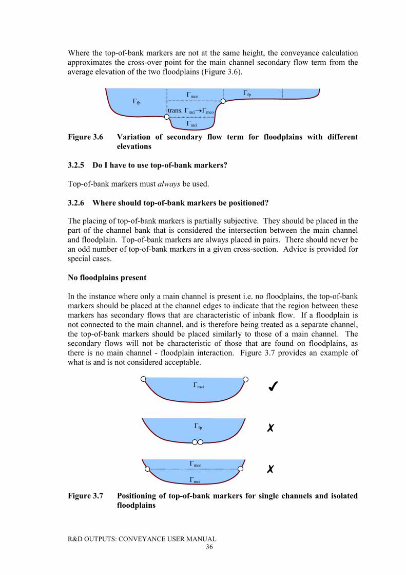
R&D OUTPUTS: CONVEYANCE USER MANUAL36
Where the top-of-bank markers are not at the same height, the conveyance calculationapproximates the cross-over point for the main channel secondary flow term from theaverage elevation of the two floodplains (Figure 3.6).
�fp
�mco
�mci
�fp
trans. �mci��mco
Figure 3.6 Variation of secondary flow term for floodplains with differentelevations
3.2.5 Do I have to use top-of-bank markers?
Top-of-bank markers must always be used.
3.2.6 Where should top-of-bank markers be positioned?
The placing of top-of-bank markers is partially subjective. They should be placed in thepart of the channel bank that is considered the intersection between the main channeland floodplain. Top-of-bank markers are always placed in pairs. There should never bean odd number of top-of-bank markers in a given cross-section. Advice is provided forspecial cases.
No floodplains present
In the instance where only a main channel is present i.e. no floodplains, the top-of-bankmarkers should be placed at the channel edges to indicate that the region between thesemarkers has secondary flows that are characteristic of inbank flow. If a floodplain isnot connected to the main channel, and is therefore being treated as a separate channel,the top-of-bank markers should be placed similarly to those of a main channel. Thesecondary flows will not be characteristic of those that are found on floodplains, asthere is no main channel - floodplain interaction. Figure 3.7 provides an example ofwhat is and is not considered acceptable.
�mci �
�fp �
�mco
�mci
�
Figure 3.7 Positioning of top-of-bank markers for single channels and isolatedfloodplains
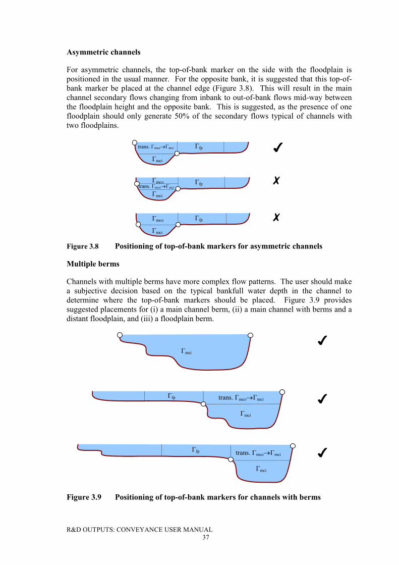
R&D OUTPUTS: CONVEYANCE USER MANUAL37
Asymmetric channels
For asymmetric channels, the top-of-bank marker on the side with the floodplain ispositioned in the usual manner. For the opposite bank, it is suggested that this top-of-bank marker be placed at the channel edge (Figure 3.8). This will result in the mainchannel secondary flows changing from inbank to out-of-bank flows mid-way betweenthe floodplain height and the opposite bank. This is suggested, as the presence of onefloodplain should only generate 50% of the secondary flows typical of channels withtwo floodplains.
�mci
�mco
�mci
�mco
�mci
�
�
�
�fp
�fp
�fp
trans. �mco��mci
trans. �mco��mci
Figure 3.8 Positioning of top-of-bank markers for asymmetric channels
Multiple berms
Channels with multiple berms have more complex flow patterns. The user should makea subjective decision based on the typical bankfull water depth in the channel todetermine where the top-of-bank markers should be placed. Figure 3.9 providessuggested placements for (i) a main channel berm, (ii) a main channel with berms and adistant floodplain, and (iii) a floodplain berm.
�mci
�
�
�trans. �mco��mci
�mci
�fp
trans. �mco��mci
�mci
�fp
Figure 3.9 Positioning of top-of-bank markers for channels with berms
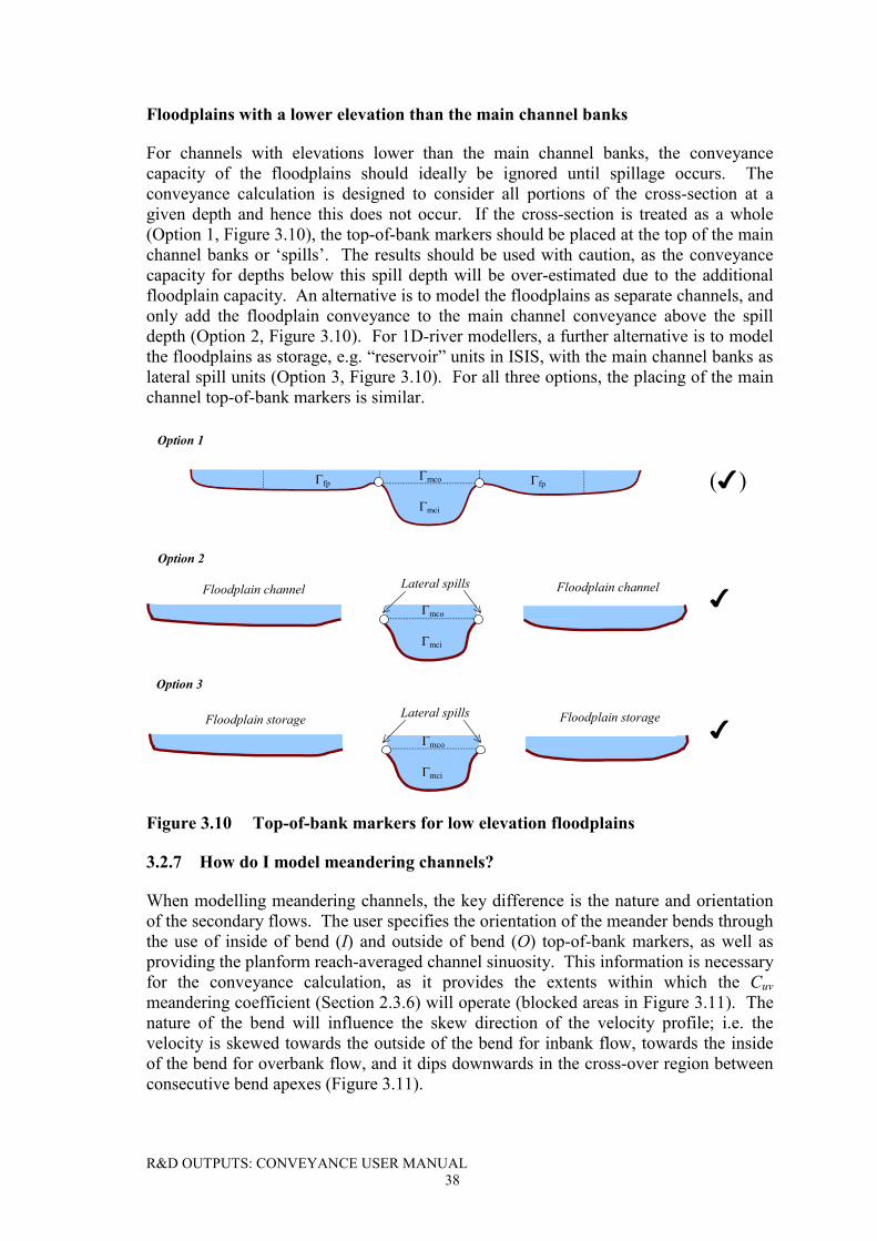
R&D OUTPUTS: CONVEYANCE USER MANUAL38
Floodplains with a lower elevation than the main channel banks
For channels with elevations lower than the main channel banks, the conveyancecapacity of the floodplains should ideally be ignored until spillage occurs. Theconveyance calculation is designed to consider all portions of the cross-section at agiven depth and hence this does not occur. If the cross-section is treated as a whole(Option 1, Figure 3.10), the top-of-bank markers should be placed at the top of the mainchannel banks or ‘spills’. The results should be used with caution, as the conveyancecapacity for depths below this spill depth will be over-estimated due to the additionalfloodplain capacity. An alternative is to model the floodplains as separate channels, andonly add the floodplain conveyance to the main channel conveyance above the spilldepth (Option 2, Figure 3.10). For 1D-river modellers, a further alternative is to modelthe floodplains as storage, e.g. “reservoir” units in ISIS, with the main channel banks aslateral spill units (Option 3, Figure 3.10). For all three options, the placing of the mainchannel top-of-bank markers is similar.
(�)
�
�
�mco
�mci
Floodplain storage Floodplain storage
�mco
�mci
Lateral spills
�mco
�mci
Lateral spillsFloodplain channel Floodplain channel
Option 3
Option 2
Option 1
�fp�fp
Figure 3.10 Top-of-bank markers for low elevation floodplains
3.2.7 How do I model meandering channels?
When modelling meandering channels, the key difference is the nature and orientationof the secondary flows. The user specifies the orientation of the meander bends throughthe use of inside of bend (I) and outside of bend (O) top-of-bank markers, as well asproviding the planform reach-averaged channel sinuosity. This information is necessaryfor the conveyance calculation, as it provides the extents within which the Cuvmeandering coefficient (Section 2.3.6) will operate (blocked areas in Figure 3.11). Thenature of the bend will influence the skew direction of the velocity profile; i.e. thevelocity is skewed towards the outside of the bend for inbank flow, towards the insideof the bend for overbank flow, and it dips downwards in the cross-over region betweenconsecutive bend apexes (Figure 3.11).
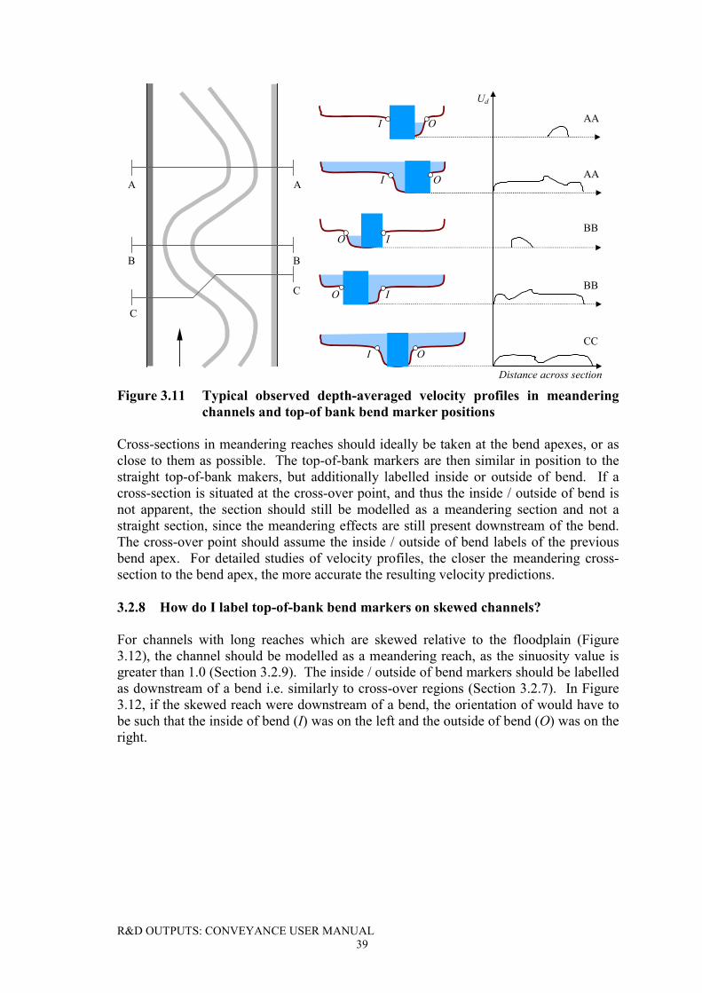
R&D OUTPUTS: CONVEYANCE USER MANUAL39
C
C
A A
B B
Ud
Distance across section
AA
BB
AA
BB
CC
I O
O I
O I
I O
I O
Figure 3.11 Typical observed depth-averaged velocity profiles in meanderingchannels and top-of bank bend marker positions
Cross-sections in meandering reaches should ideally be taken at the bend apexes, or asclose to them as possible. The top-of-bank markers are then similar in position to thestraight top-of-bank makers, but additionally labelled inside or outside of bend. If across-section is situated at the cross-over point, and thus the inside / outside of bend isnot apparent, the section should still be modelled as a meandering section and not astraight section, since the meandering effects are still present downstream of the bend.The cross-over point should assume the inside / outside of bend labels of the previousbend apex. For detailed studies of velocity profiles, the closer the meandering cross-section to the bend apex, the more accurate the resulting velocity predictions.
3.2.8 How do I label top-of-bank bend markers on skewed channels?
For channels with long reaches which are skewed relative to the floodplain (Figure3.12), the channel should be modelled as a meandering reach, as the sinuosity value isgreater than 1.0 (Section 3.2.9). The inside / outside of bend markers should be labelledas downstream of a bend i.e. similarly to cross-over regions (Section 3.2.7). In Figure3.12, if the skewed reach were downstream of a bend, the orientation of would have tobe such that the inside of bend (I) was on the left and the outside of bend (O) was on theright.
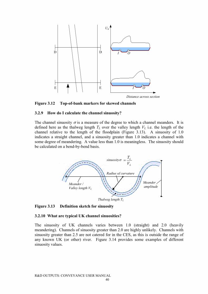
R&D OUTPUTS: CONVEYANCE USER MANUAL40
Distance across section
Ud
D D
E E
I O
I O
Figure 3.12 Top-of-bank markers for skewed channels
3.2.9 How do I calculate the channel sinuosity?
The channel sinuosity � is a measure of the degree to which a channel meanders. It isdefined here as the thalweg length TL over the valley length VL i.e. the length of thechannel relative to the length of the floodplain (Figure 3.13). A sinuosity of 1.0indicates a straight channel, and a sinuosity greater than 1.0 indicates a channel withsome degree of meandering. A value less than 1.0 is meaningless. The sinuosity shouldbe calculated on a bend-by-bend basis.
L
L
VT
�sinuosity�
Meander /Valley length VL
Thalweg length TL
Radius of curvature
Meander amplitude
Figure 3.13 Definition sketch for sinuosity
3.2.10 What are typical UK channel sinuosities?
The sinuosity of UK channels varies between 1.0 (straight) and 2.0 (heavilymeandering). Channels of sinuosity greater than 2.0 are highly unlikely. Channels withsinuosity greater than 2.5 are not catered for in the CES, as this is outside the range ofany known UK (or other) river. Figure 3.14 provides some examples of differentsinuosity values.
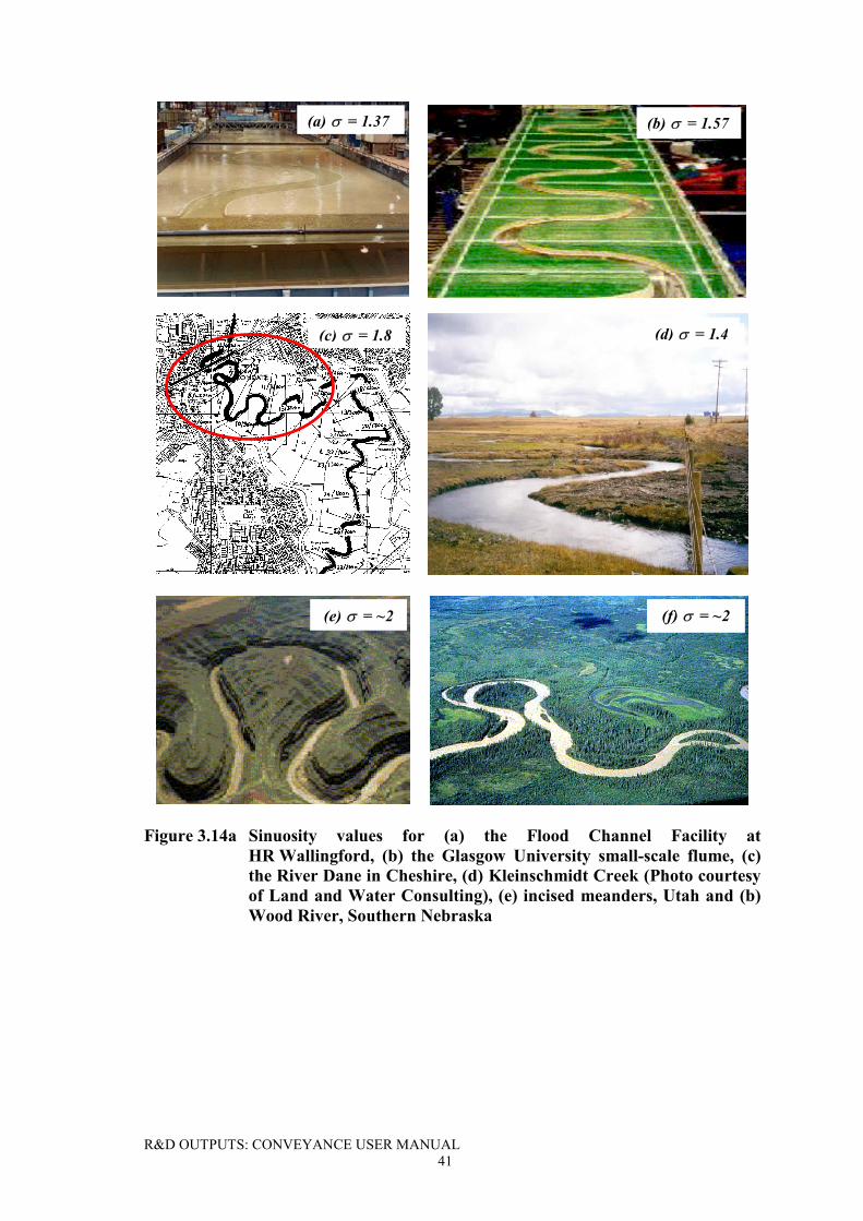
R&D OUTPUTS: CONVEYANCE USER MANUAL41
(a) � = 1.37 (b) � = 1.57
(c) � = 1.8 (d) � = 1.4
(f) � = ~2(e) � = ~2
Figure 3.14a Sinuosity values for (a) the Flood Channel Facility atHR Wallingford, (b) the Glasgow University small-scale flume, (c)the River Dane in Cheshire, (d) Kleinschmidt Creek (Photo courtesyof Land and Water Consulting), (e) incised meanders, Utah and (b)Wood River, Southern Nebraska
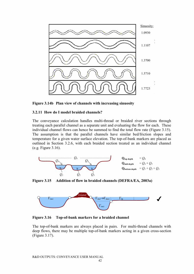
R&D OUTPUTS: CONVEYANCE USER MANUAL42
Sinuosity:
1.0930
1.1107
1.3700
1.5710
1.7723
Figure 3.14b Plan view of channels with increasing sinuosity
3.2.11 How do I model braided channels?
The conveyance calculation handles multi-thread or braided river sections throughtreating each parallel channel as a separate unit and evaluating the flow for each. Theseindividual channel flows can hence be summed to find the total flow rate (Figure 3.15).The assumption is that the parallel channels have similar bed/friction slopes andtemperature for a given water surface elevation. The top-of-bank markers are placed asoutlined in Section 3.2.6, with each braided section treated as an individual channel(e.g. Figure 3.16).
Qtop depth = Q6
Qmid-depth = Q4 + Q5
Qbottom depth = Q1 + Q2 + Q3
Q4 Q5
Q6
Q1 Q2 Q3
Figure 3.15 Addition of flow in braided channels (DEFRA/EA, 2003a)
�mci �mci��mco �fp
�mci
Island�
Figure 3.16 Top-of-bank markers for a braided channel
The top-of-bank markers are always placed in pairs. For multi-thread channels withdeep flows, there may be multiple top-of-bank markers acting in a given cross-section(Figure 3.17).
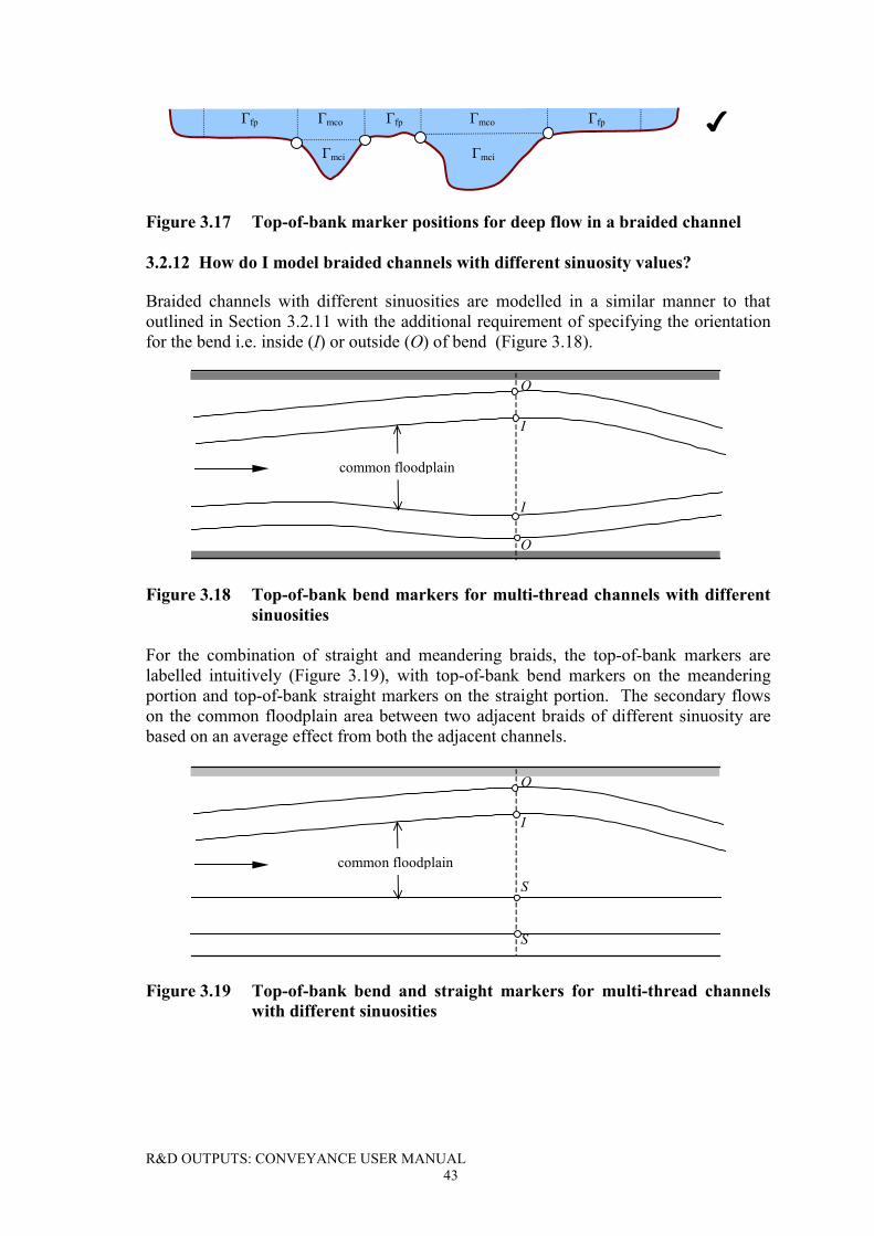
R&D OUTPUTS: CONVEYANCE USER MANUAL43
�fp �mco �fp �mco �fp
�mci �mci
�
Figure 3.17 Top-of-bank marker positions for deep flow in a braided channel
3.2.12 How do I model braided channels with different sinuosity values?
Braided channels with different sinuosities are modelled in a similar manner to thatoutlined in Section 3.2.11 with the additional requirement of specifying the orientationfor the bend i.e. inside (I) or outside (O) of bend (Figure 3.18).
O
I
I
O
common floodplain
Figure 3.18 Top-of-bank bend markers for multi-thread channels with differentsinuosities
For the combination of straight and meandering braids, the top-of-bank markers arelabelled intuitively (Figure 3.19), with top-of-bank bend markers on the meanderingportion and top-of-bank straight markers on the straight portion. The secondary flowson the common floodplain area between two adjacent braids of different sinuosity arebased on an average effect from both the adjacent channels.
common floodplain
O
I
S
S
Figure 3.19 Top-of-bank bend and straight markers for multi-thread channelswith different sinuosities
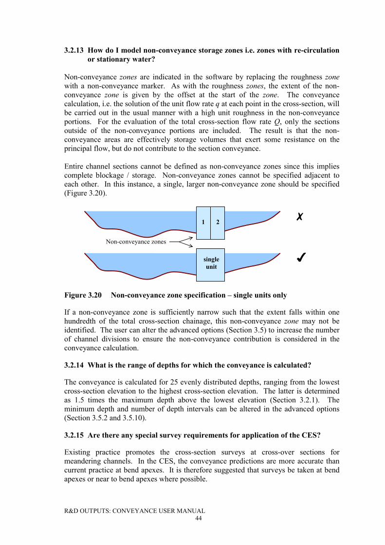
R&D OUTPUTS: CONVEYANCE USER MANUAL44
3.2.13 How do I model non-conveyance storage zones i.e. zones with re-circulationor stationary water?
Non-conveyance zones are indicated in the software by replacing the roughness zonewith a non-conveyance marker. As with the roughness zones, the extent of the non-conveyance zone is given by the offset at the start of the zone. The conveyancecalculation, i.e. the solution of the unit flow rate q at each point in the cross-section, willbe carried out in the usual manner with a high unit roughness in the non-conveyanceportions. For the evaluation of the total cross-section flow rate Q, only the sectionsoutside of the non-conveyance portions are included. The result is that the non-conveyance areas are effectively storage volumes that exert some resistance on theprincipal flow, but do not contribute to the section conveyance.
Entire channel sections cannot be defined as non-conveyance zones since this impliescomplete blockage / storage. Non-conveyance zones cannot be specified adjacent toeach other. In this instance, a single, larger non-conveyance zone should be specified(Figure 3.20).
�
�
Non-conveyance zones
1 2
singleunit
Figure 3.20 Non-conveyance zone specification – single units only
If a non-conveyance zone is sufficiently narrow such that the extent falls within onehundredth of the total cross-section chainage, this non-conveyance zone may not beidentified. The user can alter the advanced options (Section 3.5) to increase the numberof channel divisions to ensure the non-conveyance contribution is considered in theconveyance calculation.
3.2.14 What is the range of depths for which the conveyance is calculated?
The conveyance is calculated for 25 evenly distributed depths, ranging from the lowestcross-section elevation to the highest cross-section elevation. The latter is determinedas 1.5 times the maximum depth above the lowest elevation (Section 3.2.1). Theminimum depth and number of depth intervals can be altered in the advanced options(Section 3.5.2 and 3.5.10).
3.2.15 Are there any special survey requirements for application of the CES?
Existing practice promotes the cross-section surveys at cross-over sections formeandering channels. In the CES, the conveyance predictions are more accurate thancurrent practice at bend apexes. It is therefore suggested that surveys be taken at bendapexes or near to bend apexes where possible.
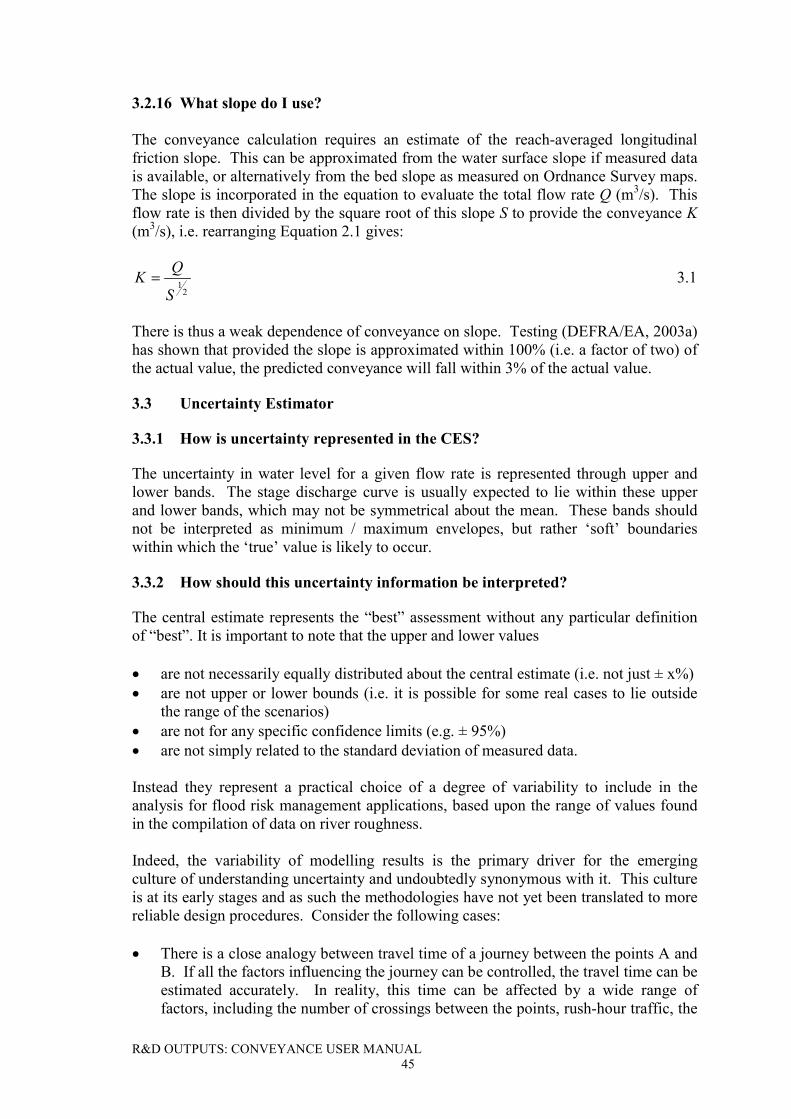
R&D OUTPUTS: CONVEYANCE USER MANUAL45
3.2.16 What slope do I use?
The conveyance calculation requires an estimate of the reach-averaged longitudinalfriction slope. This can be approximated from the water surface slope if measured datais available, or alternatively from the bed slope as measured on Ordnance Survey maps.The slope is incorporated in the equation to evaluate the total flow rate Q (m3/s). Thisflow rate is then divided by the square root of this slope S to provide the conveyance K(m3/s), i.e. rearranging Equation 2.1 gives:
21
S
QK � 3.1
There is thus a weak dependence of conveyance on slope. Testing (DEFRA/EA, 2003a)has shown that provided the slope is approximated within 100% (i.e. a factor of two) ofthe actual value, the predicted conveyance will fall within 3% of the actual value.
3.3 Uncertainty Estimator
3.3.1 How is uncertainty represented in the CES?
The uncertainty in water level for a given flow rate is represented through upper andlower bands. The stage discharge curve is usually expected to lie within these upperand lower bands, which may not be symmetrical about the mean. These bands shouldnot be interpreted as minimum / maximum envelopes, but rather ‘soft’ boundarieswithin which the ‘true’ value is likely to occur.
3.3.2 How should this uncertainty information be interpreted?
The central estimate represents the “best” assessment without any particular definitionof “best”. It is important to note that the upper and lower values
� are not necessarily equally distributed about the central estimate (i.e. not just ± x%)� are not upper or lower bounds (i.e. it is possible for some real cases to lie outside
the range of the scenarios)� are not for any specific confidence limits (e.g. ± 95%)� are not simply related to the standard deviation of measured data.
Instead they represent a practical choice of a degree of variability to include in theanalysis for flood risk management applications, based upon the range of values foundin the compilation of data on river roughness.
Indeed, the variability of modelling results is the primary driver for the emergingculture of understanding uncertainty and undoubtedly synonymous with it. This cultureis at its early stages and as such the methodologies have not yet been translated to morereliable design procedures. Consider the following cases:
� There is a close analogy between travel time of a journey between the points A andB. If all the factors influencing the journey can be controlled, the travel time can beestimated accurately. In reality, this time can be affected by a wide range offactors, including the number of crossings between the points, rush-hour traffic, the
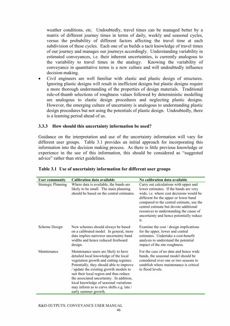
R&D OUTPUTS: CONVEYANCE USER MANUAL46
weather conditions, etc. Undoubtedly, travel times can be managed better by amatrix of different journey times in terms of daily, weekly and seasonal cycles,versus the probability of different factors affecting the travel time at eachsubdivision of these cycles. Each one of us builds a tacit knowledge of travel timesof our journey and manages our journeys accordingly. Understanding variability inestimated conveyances, i.e. their inherent uncertainties, is currently analogous tothe variability to travel times in the analogy. Knowing the variability ofconveyance in quantitative terms is a new culture and will undoubtedly influencedecision-making.
� Civil engineers are well familiar with elastic and plastic design of structures.Ignoring plastic designs will result in inefficient designs but plastic designs requirea more thorough understanding of the properties of design materials. Traditionalrule-of-thumb selections of roughness values followed by deterministic modellingare analogous to elastic design procedures and neglecting plastic designs.However, the emerging culture of uncertainty is analogous to understanding plasticdesign procedures but not using the potentials of plastic design. Undoubtedly, thereis a learning period ahead of us.
3.3.3 How should this uncertainty information be used?
Guidance on the interpretation and use of the uncertainty information will vary fordifferent user groups. Table 3.1 provides an initial approach for incorporating thisinformation into the decision making process. As there is little previous knowledge orexperience in the use of this information, this should be considered as “suggestedadvice” rather than strict guidelines.
Table 3.1 Use of uncertainty information for different user groups
User community Calibration data available No calibration data availableStrategic Planning Where data is available, the bands are
likely to be small. The main planningshould be based on the central estimates.
Carry out calculations with upper andlower estimates. If the bands are verywide, i.e. where cost decisions would bedifferent for the upper or lower bandcompared to the central estimate, use thecentral estimate but devote additionalresources to understanding the cause ofuncertainty and hence potentially reduceit.
Scheme Design New schemes should always be basedon a calibrated model. In general, moredata implies narrower uncertainty bandwidths and hence reduced freeboarddesign.
Examine the cost / design implicationsfor the upper, lower and centralestimates. Undertake a cost-benefitanalysis to understand the potentialimpact of the site roughness.
Maintenance Maintenance users are likely to havedetailed local knowledge of the localvegetation growth and cutting regimes.Potentially, they should able to improve/ update the existing growth models tosuit their local region and thus reducethe associated uncertainty. In addition,local knowledge of seasonal variationsmay inform as to curve shifts e.g. late /early summer growth.
For the case of no data and hence widebands, the seasonal model should beconsidered over one or two seasons toestablish where maintenance is criticalto flood levels.
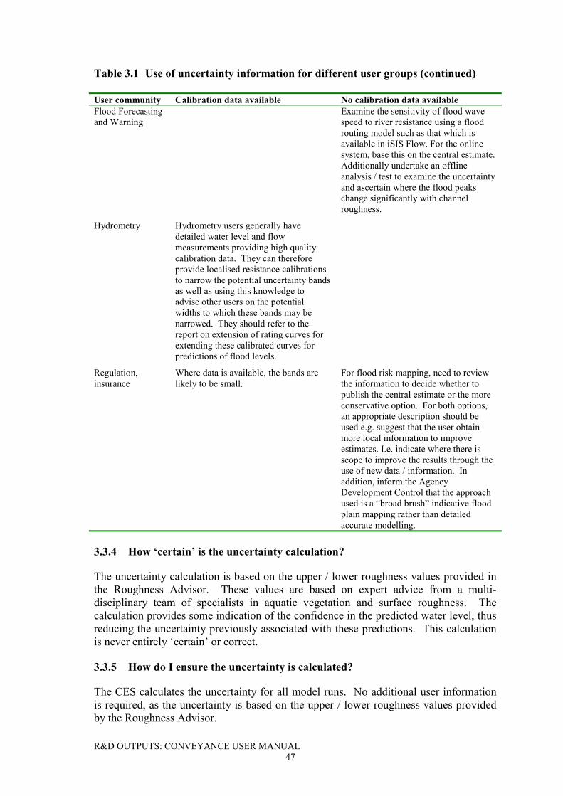
R&D OUTPUTS: CONVEYANCE USER MANUAL47
Table 3.1 Use of uncertainty information for different user groups (continued)
User community Calibration data available No calibration data availableFlood Forecastingand Warning
Examine the sensitivity of flood wavespeed to river resistance using a floodrouting model such as that which isavailable in iSIS Flow. For the onlinesystem, base this on the central estimate.Additionally undertake an offlineanalysis / test to examine the uncertaintyand ascertain where the flood peakschange significantly with channelroughness.
Hydrometry Hydrometry users generally havedetailed water level and flowmeasurements providing high qualitycalibration data. They can thereforeprovide localised resistance calibrationsto narrow the potential uncertainty bandsas well as using this knowledge toadvise other users on the potentialwidths to which these bands may benarrowed. They should refer to thereport on extension of rating curves forextending these calibrated curves forpredictions of flood levels.
Regulation,insurance
Where data is available, the bands arelikely to be small.
For flood risk mapping, need to reviewthe information to decide whether topublish the central estimate or the moreconservative option. For both options,an appropriate description should beused e.g. suggest that the user obtainmore local information to improveestimates. I.e. indicate where there isscope to improve the results through theuse of new data / information. Inaddition, inform the AgencyDevelopment Control that the approachused is a “broad brush” indicative floodplain mapping rather than detailedaccurate modelling.
3.3.4 How ‘certain’ is the uncertainty calculation?
The uncertainty calculation is based on the upper / lower roughness values provided inthe Roughness Advisor. These values are based on expert advice from a multi-disciplinary team of specialists in aquatic vegetation and surface roughness. Thecalculation provides some indication of the confidence in the predicted water level, thusreducing the uncertainty previously associated with these predictions. This calculationis never entirely ‘certain’ or correct.
3.3.5 How do I ensure the uncertainty is calculated?
The CES calculates the uncertainty for all model runs. No additional user informationis required, as the uncertainty is based on the upper / lower roughness values providedby the Roughness Advisor.
R&D OUTPUTS: CONVEYANCE USER MANUAL48
3.4 Calibration and interpretation of results
3.4.1 How do I calibrate my model and what do I change when the data does notfit?
Model calibration is fairly subjective. It depends on the channel characteristics (simple/ compound, straight / meandering), the available information, the quality of the data,availability of stage-flow calibration data and the influence of backwater effects.
For calibration within the CES environment, it is suggested that the internal modelparameters such as the dimensionless eddy viscosity � and the secondary flowparameters �mci, �mco and �fp are not altered. These parameters have been subjected torigorous testing and are set at the optimum performance values.
The calibration in straight channels is therefore based on altering the roughness zonesi.e. roughness magnitudes and extents; and altering the positioning of the top-of-bankmarkers to best capture the bankfull secondary flow transition characteristics. Inmeandering channels, in addition to the above, the magnitude of the sinuosity can bealtered within a reasonable range for the site concerned.
The water levels should be most sensitive to variations in roughness, while the top-of-bank markers and sinuosity magnitude effect the bankfull depths and main channel flowrespectively.
If calibration is not achieved, other alternatives include re-evaluating and checking theinput data e.g. longitudinal reach-averaged bed slope and survey data.
3.4.2 Why do I get jumps in the conveyance curve at sudden geometry changese.g. bankfull?
At bankfull, the secondary flow model changes from representing the secondarycirculations characteristic of inbank flow, to those characteristic of out-of-bank flow(Section 2.3.6). The energy transfer mechanisms change and in some instances thisresults in a ‘jump’ in the stage-discharge curve at bankfull (e.g. Figure 3.21). Thisphysical phenomenon can be observed in real channels e.g. River Severn at MontfordBridge (DEFRA/EA, 2003a). Varying the top-of-bank marker positions can alter the‘jump’ level.
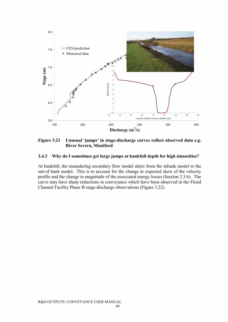
R&D OUTPUTS: CONVEYANCE USER MANUAL49
5.5
6.0
6.5
7.0
7.5
8.0
150 200 250 300 350 400
Discharge (m3/s)
Stag
e (m
)CES predictionMeasured data
0
1
2
3
4
5
6
7
8
9
10
-10 10 30 50 70 90 110 130 150
Lateral distance across channel (m)
Bed
leve
l (m
)
Figure 3.21 Unusual ‘jumps’ in stage-discharge curves reflect observed data e.g.River Severn, Montford
3.4.3 Why do I sometimes get large jumps at bankfull depth for high sinuosities?
At bankfull, the meandering secondary flow model alters from the inbank model to theout-of bank model. This is to account for the change in expected skew of the velocityprofile and the change in magnitude of the associated energy losses (Section 2.3.6). Thecurve may have sharp reductions in conveyance which have been observed in the FloodChannel Facility Phase B stage-discharge observations (Figure 3.22).
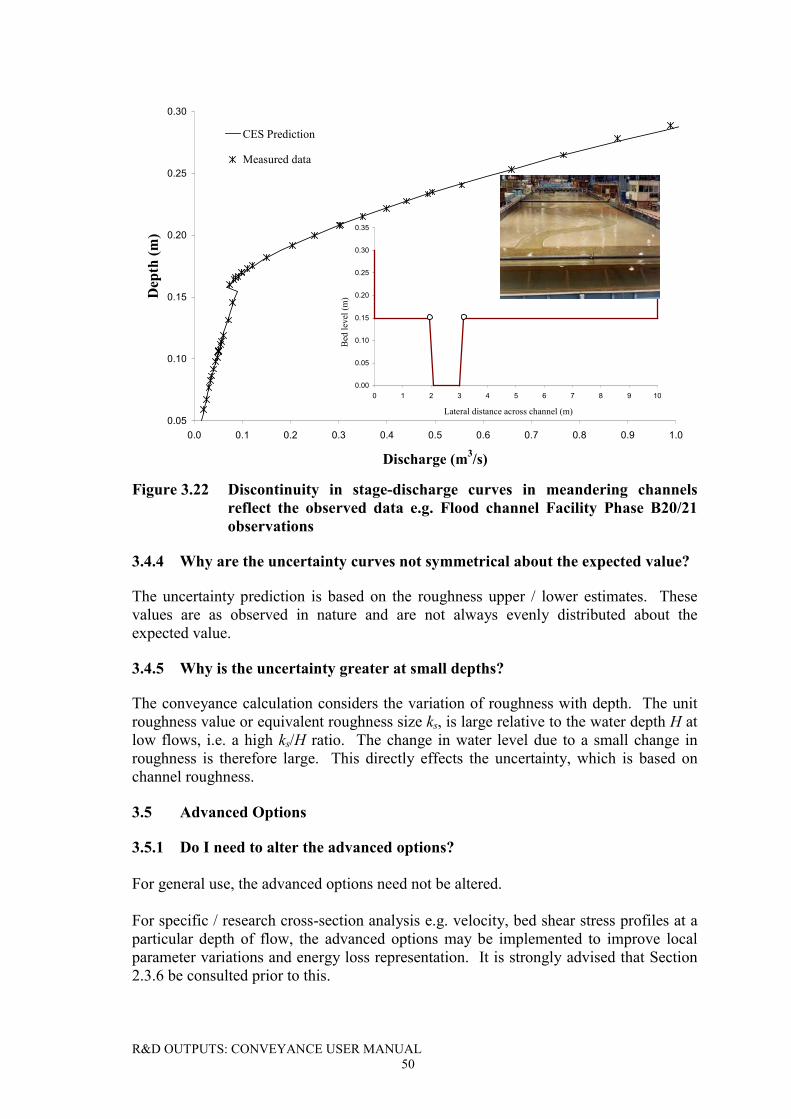
R&D OUTPUTS: CONVEYANCE USER MANUAL50
0.05
0.10
0.15
0.20
0.25
0.30
0.0 0.1 0.2 0.3 0.4 0.5 0.6 0.7 0.8 0.9 1.0
Discharge (m3/s)
Dep
th (m
)CES Prediction
Measured data
0.00
0.05
0.10
0.15
0.20
0.25
0.30
0.35
0 1 2 3 4 5 6 7 8 9 10
Lateral distance across channel (m)
Bed
leve
l (m
)
Figure 3.22 Discontinuity in stage-discharge curves in meandering channelsreflect the observed data e.g. Flood channel Facility Phase B20/21observations
3.4.4 Why are the uncertainty curves not symmetrical about the expected value?
The uncertainty prediction is based on the roughness upper / lower estimates. Thesevalues are as observed in nature and are not always evenly distributed about theexpected value.
3.4.5 Why is the uncertainty greater at small depths?
The conveyance calculation considers the variation of roughness with depth. The unitroughness value or equivalent roughness size ks, is large relative to the water depth H atlow flows, i.e. a high ks/H ratio. The change in water level due to a small change inroughness is therefore large. This directly effects the uncertainty, which is based onchannel roughness.
3.5 Advanced Options
3.5.1 Do I need to alter the advanced options?
For general use, the advanced options need not be altered.
For specific / research cross-section analysis e.g. velocity, bed shear stress profiles at aparticular depth of flow, the advanced options may be implemented to improve localparameter variations and energy loss representation. It is strongly advised that Section2.3.6 be consulted prior to this.
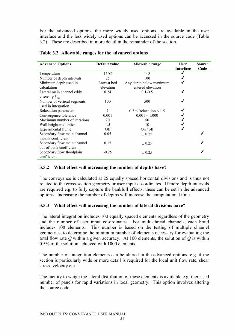
R&D OUTPUTS: CONVEYANCE USER MANUAL51
For the advanced options, the more widely used options are available in the userinterface and the less widely used options can be accessed in the source code (Table3.2). These are described in more detail in the remainder of the section.
Table 3.2 Allowable ranges for the advanced options
Advanced Options Default value Allowable range UserInterface
SourceCode
Temperature 15�C > 0 �
Number of depth intervals 25 100 �
Minimum depth used incalculation
Lowest bedelevation
Any depth below maximumentered elevation
�
Lateral main channel eddyviscosity �mc
0.24 0.1-0.5 �
Number of vertical segmentsused in integration
100 500 �
Relaxation parameter 1 0.5 � Relaxation � 1.5 �
Convergence tolerance 0.001 0.001 – 1.000 �
Maximum number of iterations 20 50 �
Wall height multiplier 1.5 10 �
Experimental flume Off On / off �
Secondary flow main channelinbank coefficient
0.05 � 0.25 �
Secondary flow main channelout-of-bank coefficient
0.15 � 0.25 �
Secondary flow floodplaincoefficient
-0.25 � 0.25 �
3.5.2 What effect will increasing the number of depths have?
The conveyance is calculated at 25 equally spaced horizontal divisions and is thus notrelated to the cross-section geometry or user input co-ordinates. If more depth intervalsare required e.g. to fully capture the bankfull effects, these can be set in the advancedoptions. Increasing the number of depths will increase the computational time.
3.5.3 What effect will increasing the number of lateral divisions have?
The lateral integration includes 100 equally spaced elements regardless of the geometryand the number of user input co-ordinates. For multi-thread channels, each braidincludes 100 elements. This number is based on the testing of multiple channelgeometries, to determine the minimum number of elements necessary for evaluating thetotal flow rate Q within a given accuracy. At 100 elements, the solution of Q is within0.5% of the solution achieved with 1000 elements.
The number of integration elements can be altered in the advanced options, e.g. if thesection is particularly wide or more detail is required for the local unit flow rate, shearstress, velocity etc.
The facility to weigh the lateral distribution of these elements is available e.g. increasednumber of panels for rapid variations in local geometry. This option involves alteringthe source code.
R&D OUTPUTS: CONVEYANCE USER MANUAL52
3.5.4 What happens if I change the dimensionless eddy viscosity?
The dimensionless eddy viscosity � represents the amount of lateral spread due toboundary or shear layer effects. In the literature (Knight and Shiono, 1990; Knight andShiono 1991; James and Wark, 1992), values are typically in the range 0.07(experimental facilities) to 0.5 (natural channels). The model is based on the mainchannel value, �mc, which can be altered from the default 0.24 in the advanced options.Values less than 0.1 may cause convergence difficulties. Values greater than 0.5represent a large amount of lateral momentum exchange, and are highly unlikely.
It is advised that this parameter is not altered other than for academic purposes.
3.5.5 What happens if I change the straight secondary flow coefficients?
Altering the straight secondary flow coefficients, �mci, �mco and �fp (Section 2.3.6)requires access to the source code. The default values are 0.05, 0.15 and –0.25. Thesecan be altered within the range �0.25. The effect is to uniformly increase / decrease theenergy losses in the appropriate flow region (Section 3.2.4).
3.5.6 What happens if I alter the temperature?
Altering the temperature from the default 15 �C will have little impact. For naturalcross-sections, the CES analysis does not use the temperature. For experimental flumes,the temperature is used to determine viscosity � for the Colebrook-White equation, i.e.(Raudkivi, 1998),
62 10)T00066.0T0499.0741.1( �
����� 3.2
3.5.7 What happens if I alter the relaxation parameter?
The default relaxation parameter � is set at 1.0. This value may be varied between 0.5<� �1.5, and always less than 2.0. The relaxation is used to update the correctionparameter �q in the iteration process,
nnn qqq ����
�1 3.3
where n is the iteration number i.e. it affects the value of successive approximations tothe actual solution. The relaxation should never be zero, as this will eliminate theiterative procedure i.e. successive q guesses will be identical (qn = qn+1). A negativerelaxation is not advised, as this eliminates the sign of the suggested correction from theprevious iteration e.g. if �q = –0.001m2/s, and the relaxation is –1, this implies acorrection of +0.001m2/s, which will not support convergence. Altering the relaxationwill affect the number of iterations taken to reach the solution. The relaxation does notaffect the results i.e. the actual water level predictions.
The relaxation is altered internally for the rare case where �qn < 0 and |�qn| qn , toensure that the updated qn+1 is positive. This is critical for numerical stability, as theunit flow rate appears within the log function in the Colebrook-White friction law. It isalso physically meaningless as it implies upstream flow.
R&D OUTPUTS: CONVEYANCE USER MANUAL53
3.5.8 If I alter an advanced parameter, does the change apply to that cross-section only?
Yes. The software is designed such that the advanced parameters for each cross-sectioncan be described and applied individually.
3.5.9 What happens if I set the minimum depth?
The minimum depth enables the user to enter a specific depth for the first and lowest ofthe 25 depths that are solved for. The range of calculation depths will extend from thisminimum depth to the maximum depth (defined Section 3.2.1).
3.5.10 Why would I set the minimum depth?
This is a useful tool if the user is interested in the flow parameters for a specific depth.The default calculation always provides the results for 25 equally spaced depths thatmay not coincide with the depth of interest.
3.5.11 What does the wall height multiplier do?
The wall height multiplier represents the amount that the maximum cross-section depthis multiplied by to determine the maximum depth for calculation (Section 3.2.1). Thedefault value is 1.5. This can be altered to any number greater than 1.0. A value greaterthan 1.5 would imply that very large flows and depths are anticipated. If both low andvery high flows are of interest, then both wall height multiplier and the number of depthintervals should be increased.
3.5.12 What happens if I alter the maximum number of iterations?
The default maximum number of iterations is 20. This represents the maximumallowable iterations of Equation 2.6a and b to solve q within the required tolerance of0.001m2/s. The solution is designed to converge nearly quadratically, and is thereforeunlikely to take more than 5-7 iterations. In rare instances, e.g. sections with rapidlyvarying local roughness, the solution may take longer to converge. Increasing thenumber of iterations to 25 or 30 may marginally improve the results.
3.5.13 What does the experimental flume option change?
For modelling experimental flumes, this option should be selected. The ConveyanceGenerator will then use the full Colebrook-White equation (Section 2.3.6), i.e. bothsmooth and rough laws, for determining the lateral distribution of f. The distribution off is thus dependent on both the roughness size and the localised velocity, as is expectedfor laboratory flume flow.
3.5.14 What does the convergence tolerance change?
The convergence tolerance is used in the iterative calculation for determining how closethe approximation to the unit flow rate q (m2/s) is to the previous iteration. Once therequired tolerance is achieved (default 0.001 m2/s), the solution is assumed to haveconverged. In rare cases where the river is extremely wide, this tolerance may never beachieved. It is thus possible to increase the tolerance up to a value of 1.0 to ensure a
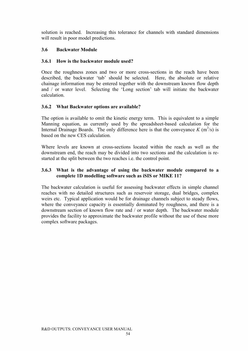
R&D OUTPUTS: CONVEYANCE USER MANUAL54
solution is reached. Increasing this tolerance for channels with standard dimensionswill result in poor model predictions.
3.6 Backwater Module
3.6.1 How is the backwater module used?
Once the roughness zones and two or more cross-sections in the reach have beendescribed, the backwater ‘tab’ should be selected. Here, the absolute or relativechainage information may be entered together with the downstream known flow depthand / or water level. Selecting the ‘Long section’ tab will initiate the backwatercalculation.
3.6.2 What Backwater options are available?
The option is available to omit the kinetic energy term. This is equivalent to a simpleManning equation, as currently used by the spreadsheet-based calculation for theInternal Drainage Boards. The only difference here is that the conveyance K (m3/s) isbased on the new CES calculation.
Where levels are known at cross-sections located within the reach as well as thedownstream end, the reach may be divided into two sections and the calculation is re-started at the split between the two reaches i.e. the control point.
3.6.3 What is the advantage of using the backwater module compared to acomplete 1D modelling software such as iSIS or MIKE 11?
The backwater calculation is useful for assessing backwater effects in simple channelreaches with no detailed structures such as reservoir storage, dual bridges, complexweirs etc. Typical application would be for drainage channels subject to steady flows,where the conveyance capacity is essentially dominated by roughness, and there is adownstream section of known flow rate and / or water depth. The backwater moduleprovides the facility to approximate the backwater profile without the use of these morecomplex software packages.
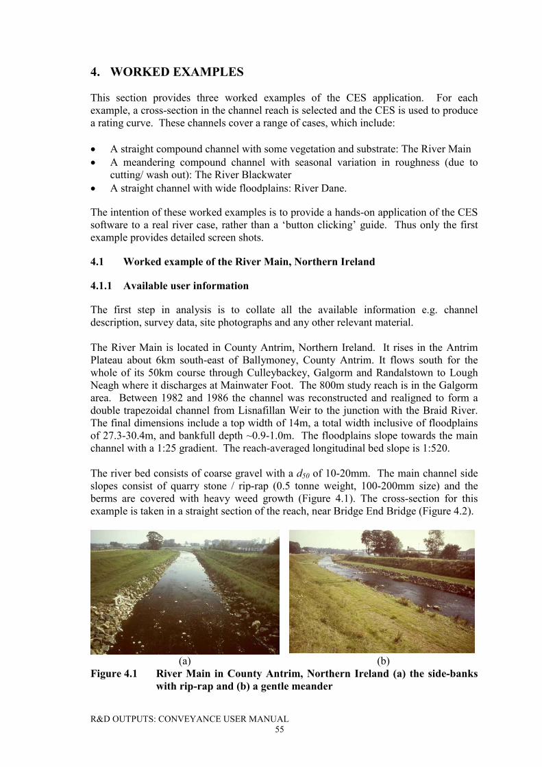
R&D OUTPUTS: CONVEYANCE USER MANUAL55
4. WORKED EXAMPLES
This section provides three worked examples of the CES application. For eachexample, a cross-section in the channel reach is selected and the CES is used to producea rating curve. These channels cover a range of cases, which include:
� A straight compound channel with some vegetation and substrate: The River Main� A meandering compound channel with seasonal variation in roughness (due to
cutting/ wash out): The River Blackwater� A straight channel with wide floodplains: River Dane.
The intention of these worked examples is to provide a hands-on application of the CESsoftware to a real river case, rather than a ‘button clicking’ guide. Thus only the firstexample provides detailed screen shots.
4.1 Worked example of the River Main, Northern Ireland
4.1.1 Available user information
The first step in analysis is to collate all the available information e.g. channeldescription, survey data, site photographs and any other relevant material.
The River Main is located in County Antrim, Northern Ireland. It rises in the AntrimPlateau about 6km south-east of Ballymoney, County Antrim. It flows south for thewhole of its 50km course through Culleybackey, Galgorm and Randalstown to LoughNeagh where it discharges at Mainwater Foot. The 800m study reach is in the Galgormarea. Between 1982 and 1986 the channel was reconstructed and realigned to form adouble trapezoidal channel from Lisnafillan Weir to the junction with the Braid River.The final dimensions include a top width of 14m, a total width inclusive of floodplainsof 27.3-30.4m, and bankfull depth ~0.9-1.0m. The floodplains slope towards the mainchannel with a 1:25 gradient. The reach-averaged longitudinal bed slope is 1:520.
The river bed consists of coarse gravel with a d50 of 10-20mm. The main channel sideslopes consist of quarry stone / rip-rap (0.5 tonne weight, 100-200mm size) and theberms are covered with heavy weed growth (Figure 4.1). The cross-section for thisexample is taken in a straight section of the reach, near Bridge End Bridge (Figure 4.2).
(a) (b)Figure 4.1 River Main in County Antrim, Northern Ireland (a) the side-banks
with rip-rap and (b) a gentle meander
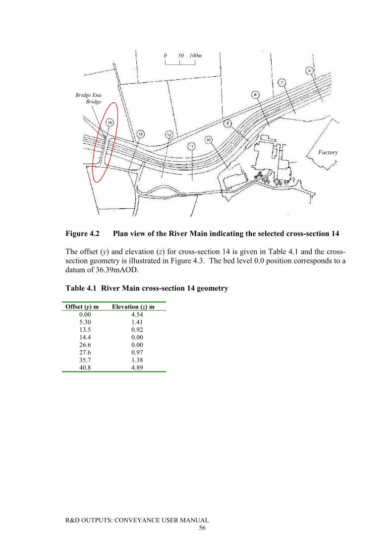
R&D OUTPUTS: CONVEYANCE USER MANUAL56
Bridge EndBridge
0 50 100m
Factory
Figure 4.2 Plan view of the River Main indicating the selected cross-section 14
The offset (y) and elevation (z) for cross-section 14 is given in Table 4.1 and the cross-section geometry is illustrated in Figure 4.3. The bed level 0.0 position corresponds to adatum of 36.39mAOD.
Table 4.1 River Main cross-section 14 geometry
Offset (y) m Elevation (z) m0.00 4.545.30 1.4113.5 0.9214.4 0.0026.6 0.0027.6 0.9735.7 1.3840.8 4.89
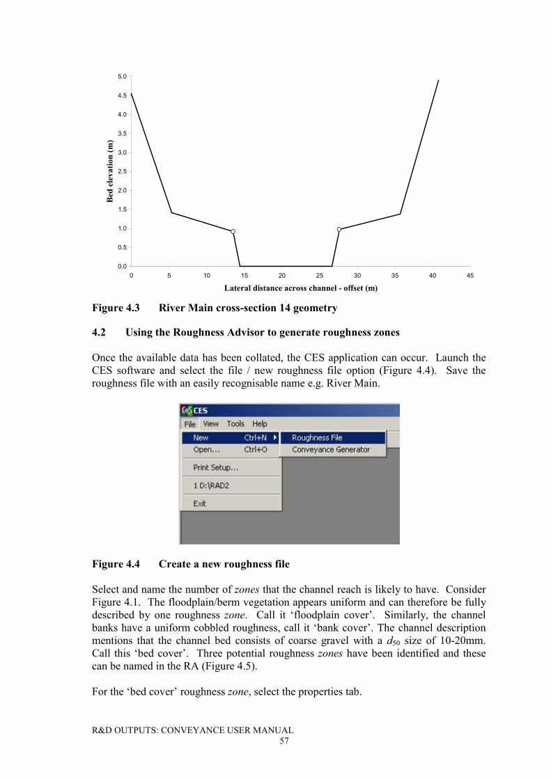
R&D OUTPUTS: CONVEYANCE USER MANUAL57
0.0
0.5
1.0
1.5
2.0
2.5
3.0
3.5
4.0
4.5
5.0
0 5 10 15 20 25 30 35 40 45
Lateral distance across channel - offset (m)
Bed
ele
vatio
n (m
)
Figure 4.3 River Main cross-section 14 geometry
4.2 Using the Roughness Advisor to generate roughness zones
Once the available data has been collated, the CES application can occur. Launch theCES software and select the file / new roughness file option (Figure 4.4). Save theroughness file with an easily recognisable name e.g. River Main.
Figure 4.4 Create a new roughness file
Select and name the number of zones that the channel reach is likely to have. ConsiderFigure 4.1. The floodplain/berm vegetation appears uniform and can therefore be fullydescribed by one roughness zone. Call it ‘floodplain cover’. Similarly, the channelbanks have a uniform cobbled roughness, call it ‘bank cover’. The channel descriptionmentions that the channel bed consists of coarse gravel with a d50 size of 10-20mm.Call this ‘bed cover’. Three potential roughness zones have been identified and thesecan be named in the RA (Figure 4.5).
For the ‘bed cover’ roughness zone, select the properties tab.
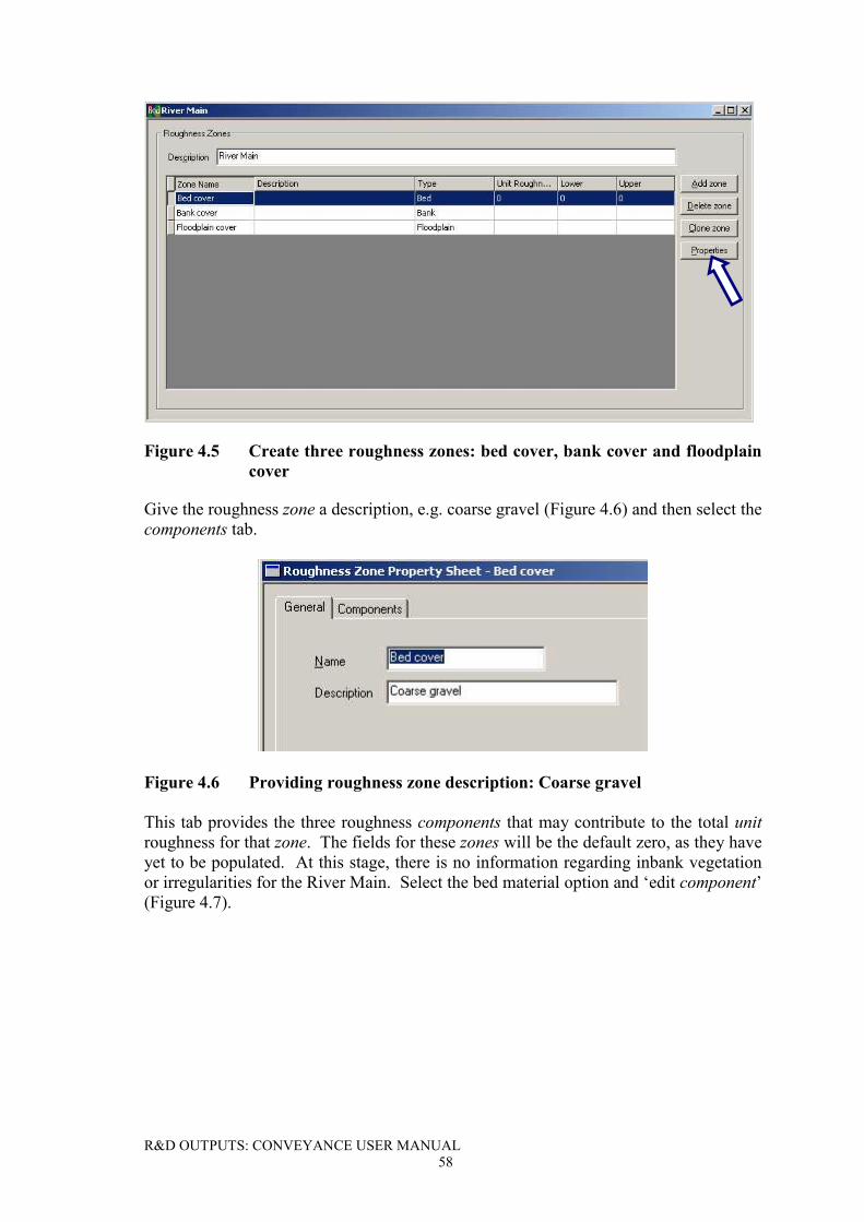
R&D OUTPUTS: CONVEYANCE USER MANUAL58
Figure 4.5 Create three roughness zones: bed cover, bank cover and floodplaincover
Give the roughness zone a description, e.g. coarse gravel (Figure 4.6) and then select thecomponents tab.
Figure 4.6 Providing roughness zone description: Coarse gravel
This tab provides the three roughness components that may contribute to the total unitroughness for that zone. The fields for these zones will be the default zero, as they haveyet to be populated. At this stage, there is no information regarding inbank vegetationor irregularities for the River Main. Select the bed material option and ‘edit component’(Figure 4.7).
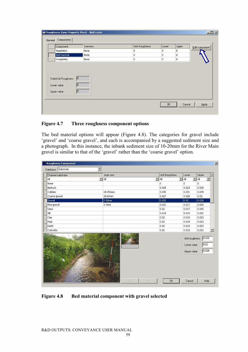
R&D OUTPUTS: CONVEYANCE USER MANUAL59
Figure 4.7 Three roughness component options
The bed material options will appear (Figure 4.8). The categories for gravel include‘gravel’ and ‘coarse gravel’, and each is accompanied by a suggested sediment size anda photograph. In this instance, the inbank sediment size of 10-20mm for the River Maingravel is similar to that of the ‘gravel’ rather than the ‘coarse gravel’ option.
Figure 4.8 Bed material component with gravel selected
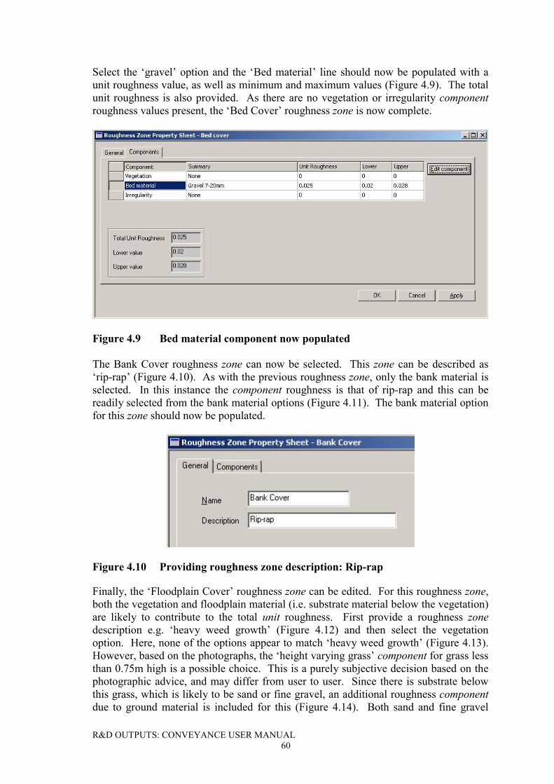
R&D OUTPUTS: CONVEYANCE USER MANUAL60
Select the ‘gravel’ option and the ‘Bed material’ line should now be populated with aunit roughness value, as well as minimum and maximum values (Figure 4.9). The totalunit roughness is also provided. As there are no vegetation or irregularity componentroughness values present, the ‘Bed Cover’ roughness zone is now complete.
Figure 4.9 Bed material component now populated
The Bank Cover roughness zone can now be selected. This zone can be described as‘rip-rap’ (Figure 4.10). As with the previous roughness zone, only the bank material isselected. In this instance the component roughness is that of rip-rap and this can bereadily selected from the bank material options (Figure 4.11). The bank material optionfor this zone should now be populated.
Figure 4.10 Providing roughness zone description: Rip-rap
Finally, the ‘Floodplain Cover’ roughness zone can be edited. For this roughness zone,both the vegetation and floodplain material (i.e. substrate material below the vegetation)are likely to contribute to the total unit roughness. First provide a roughness zonedescription e.g. ‘heavy weed growth’ (Figure 4.12) and then select the vegetationoption. Here, none of the options appear to match ‘heavy weed growth’ (Figure 4.13).However, based on the photographs, the ‘height varying grass’ component for grass lessthan 0.75m high is a possible choice. This is a purely subjective decision based on thephotographic advice, and may differ from user to user. Since there is substrate belowthis grass, which is likely to be sand or fine gravel, an additional roughness componentdue to ground material is included for this (Figure 4.14). Both sand and fine gravel
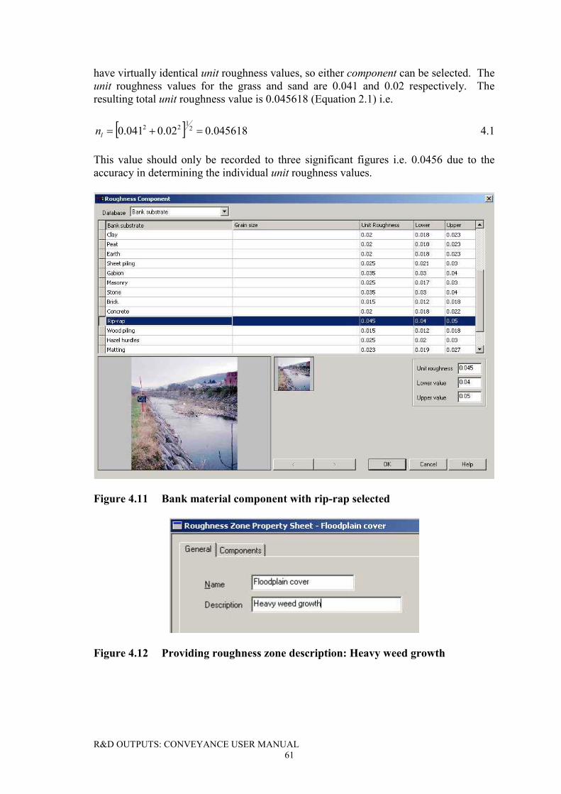
R&D OUTPUTS: CONVEYANCE USER MANUAL61
have virtually identical unit roughness values, so either component can be selected. Theunit roughness values for the grass and sand are 0.041 and 0.02 respectively. Theresulting total unit roughness value is 0.045618 (Equation 2.1) i.e.
� � 045618.002.0041.0 2122���ln 4.1
This value should only be recorded to three significant figures i.e. 0.0456 due to theaccuracy in determining the individual unit roughness values.
Figure 4.11 Bank material component with rip-rap selected
Figure 4.12 Providing roughness zone description: Heavy weed growth
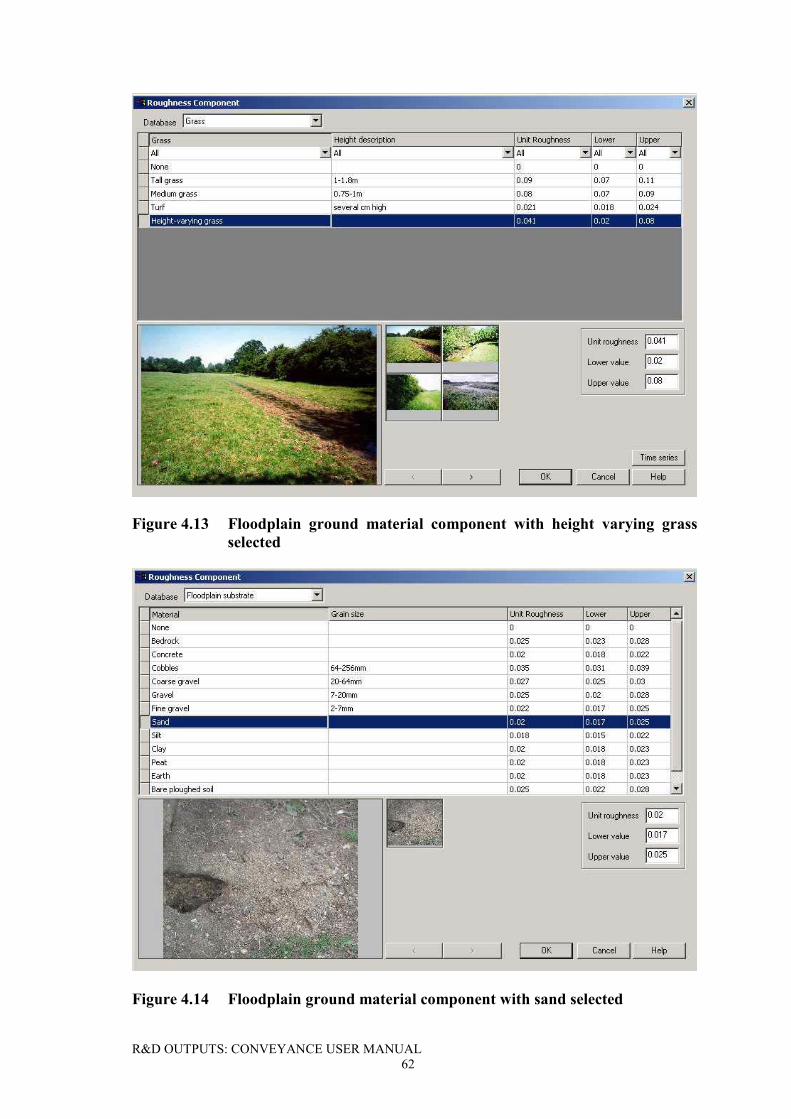
R&D OUTPUTS: CONVEYANCE USER MANUAL62
Figure 4.13 Floodplain ground material component with height varying grassselected
Figure 4.14 Floodplain ground material component with sand selected
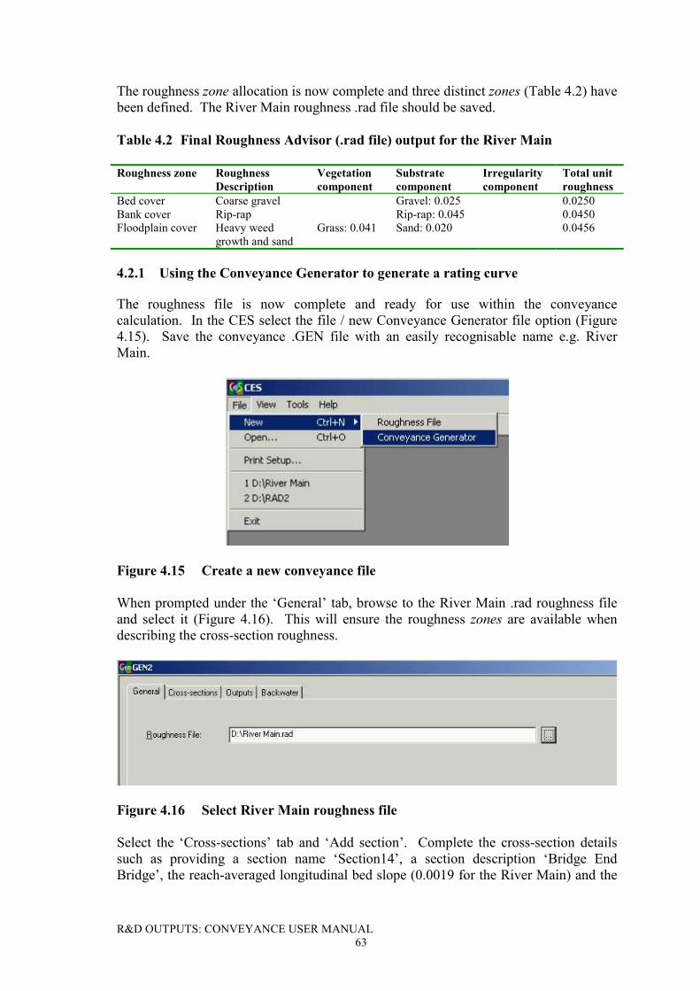
R&D OUTPUTS: CONVEYANCE USER MANUAL63
The roughness zone allocation is now complete and three distinct zones (Table 4.2) havebeen defined. The River Main roughness .rad file should be saved.
Table 4.2 Final Roughness Advisor (.rad file) output for the River Main
Roughness zone RoughnessDescription
Vegetationcomponent
Substratecomponent
Irregularitycomponent
Total unitroughness
Bed cover Coarse gravel Gravel: 0.025 0.0250Bank cover Rip-rap Rip-rap: 0.045 0.0450Floodplain cover Heavy weed
growth and sandGrass: 0.041 Sand: 0.020 0.0456
4.2.1 Using the Conveyance Generator to generate a rating curve
The roughness file is now complete and ready for use within the conveyancecalculation. In the CES select the file / new Conveyance Generator file option (Figure4.15). Save the conveyance .GEN file with an easily recognisable name e.g. RiverMain.
Figure 4.15 Create a new conveyance file
When prompted under the ‘General’ tab, browse to the River Main .rad roughness fileand select it (Figure 4.16). This will ensure the roughness zones are available whendescribing the cross-section roughness.
Figure 4.16 Select River Main roughness file
Select the ‘Cross-sections’ tab and ‘Add section’. Complete the cross-section detailssuch as providing a section name ‘Section14’, a section description ‘Bridge EndBridge’, the reach-averaged longitudinal bed slope (0.0019 for the River Main) and the
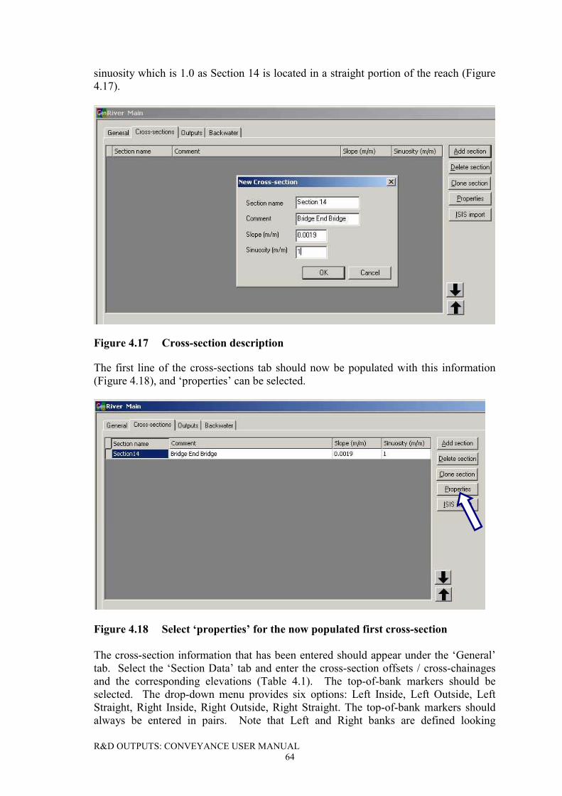
R&D OUTPUTS: CONVEYANCE USER MANUAL64
sinuosity which is 1.0 as Section 14 is located in a straight portion of the reach (Figure4.17).
Figure 4.17 Cross-section description
The first line of the cross-sections tab should now be populated with this information(Figure 4.18), and ‘properties’ can be selected.
Figure 4.18 Select ‘properties’ for the now populated first cross-section
The cross-section information that has been entered should appear under the ‘General’tab. Select the ‘Section Data’ tab and enter the cross-section offsets / cross-chainagesand the corresponding elevations (Table 4.1). The top-of-bank markers should beselected. The drop-down menu provides six options: Left Inside, Left Outside, LeftStraight, Right Inside, Right Outside, Right Straight. The top-of-bank markers shouldalways be entered in pairs. Note that Left and Right banks are defined looking
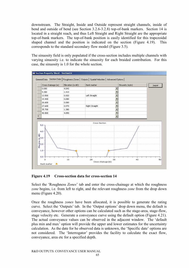
R&D OUTPUTS: CONVEYANCE USER MANUAL65
downstream. The Straight, Inside and Outside represent straight channels, inside ofbend and outside of bend (see Section 3.2.6-3.2.8) top-of-bank markers. Section 14 islocated in a straight reach, and thus Left Straight and Right Straight are the appropriatetop-of-bank markers. The top-of-bank position is easily identified for this trapezoidalshaped channel and the position is indicated on the section (Figure 4.19). Thiscorresponds to the standard secondary flow model (Figure 3.5).
The sinuosity field is only populated if the cross-section includes multiple channels withvarying sinuosity i.e. to indicate the sinuosity for each braided contribution. For thiscase, the sinuosity is 1.0 for the whole section.
Figure 4.19 Cross-section data for cross-section 14
Select the ‘Roughness Zones’ tab and enter the cross-chainage at which the roughnesszone begins, i.e. from left to right, and the relevant roughness zone from the drop downmenu (Figure 4.20).
Once the roughness zones have been allocated, it is possible to generate the ratingcurve. Select the ‘Outputs’ tab. In the ‘Output options’ drop down menu, the default isconveyance, however other options can be calculated such as the stage-area, stage-flow,stage velocity etc. Generate a conveyance curve using the default option (Figure 4.21).The actual conveyance values can be observed in the adjacent window. The ‘defaultplus min and max’ option will provide the upper and lower estimates for the uncertaintycalculation. As the date for he observed data is unknown, the ‘Specific date’ options arenot considered. The ‘Interrogator’ provides the facility to calculate the exact flow,conveyance, area etc for a specified depth.
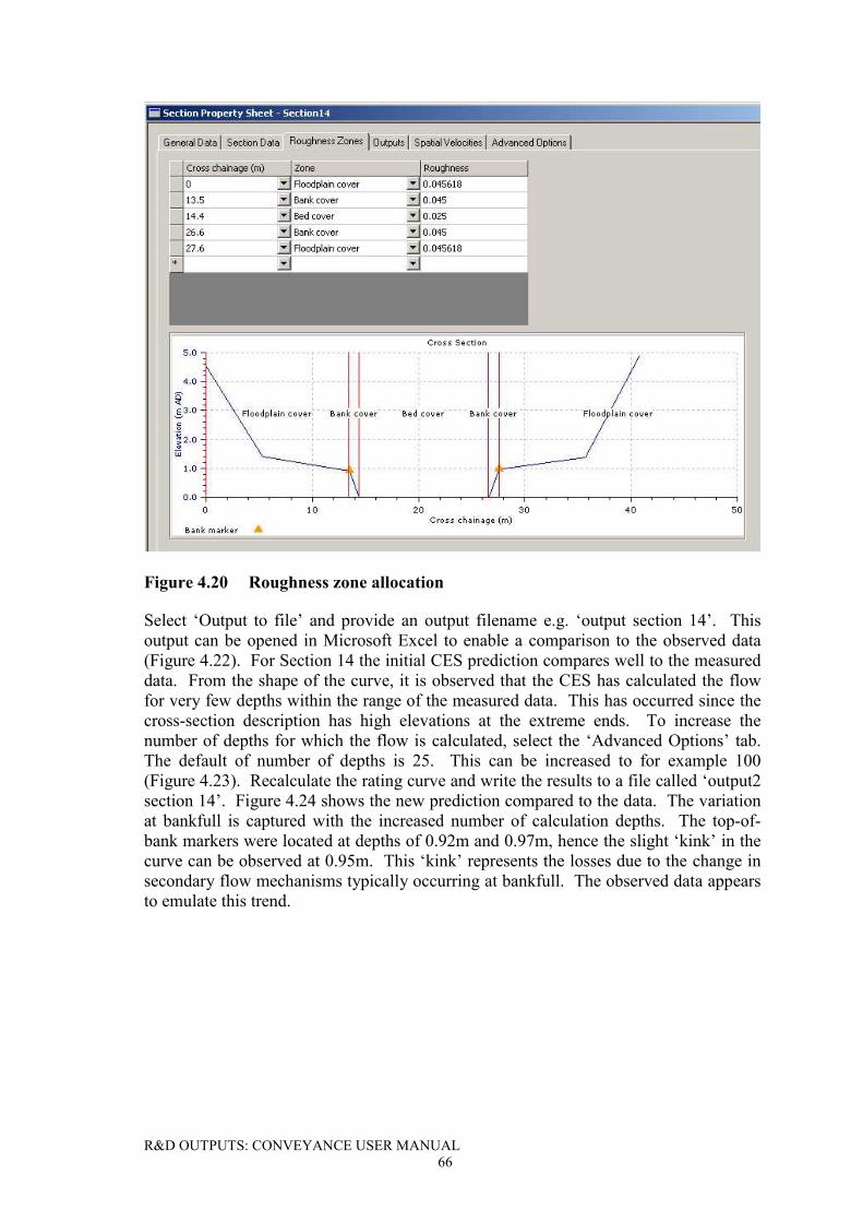
R&D OUTPUTS: CONVEYANCE USER MANUAL66
Figure 4.20 Roughness zone allocation
Select ‘Output to file’ and provide an output filename e.g. ‘output section 14’. Thisoutput can be opened in Microsoft Excel to enable a comparison to the observed data(Figure 4.22). For Section 14 the initial CES prediction compares well to the measureddata. From the shape of the curve, it is observed that the CES has calculated the flowfor very few depths within the range of the measured data. This has occurred since thecross-section description has high elevations at the extreme ends. To increase thenumber of depths for which the flow is calculated, select the ‘Advanced Options’ tab.The default of number of depths is 25. This can be increased to for example 100(Figure 4.23). Recalculate the rating curve and write the results to a file called ‘output2section 14’. Figure 4.24 shows the new prediction compared to the data. The variationat bankfull is captured with the increased number of calculation depths. The top-of-bank markers were located at depths of 0.92m and 0.97m, hence the slight ‘kink’ in thecurve can be observed at 0.95m. This ‘kink’ represents the losses due to the change insecondary flow mechanisms typically occurring at bankfull. The observed data appearsto emulate this trend.
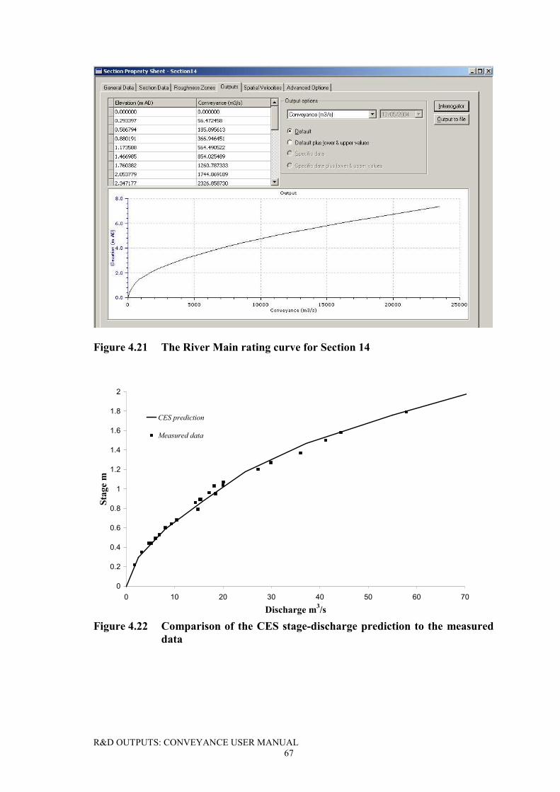
R&D OUTPUTS: CONVEYANCE USER MANUAL67
Figure 4.21 The River Main rating curve for Section 14
0
0.2
0.4
0.6
0.8
1
1.2
1.4
1.6
1.8
2
0 10 20 30 40 50 60 70
Discharge m3/s
Stag
e m
CES prediction
Measured data
Figure 4.22 Comparison of the CES stage-discharge prediction to the measureddata
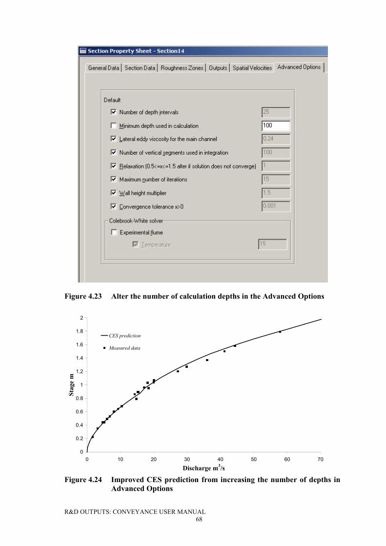
R&D OUTPUTS: CONVEYANCE USER MANUAL68
Figure 4.23 Alter the number of calculation depths in the Advanced Options
0
0.2
0.4
0.6
0.8
1
1.2
1.4
1.6
1.8
2
0 10 20 30 40 50 60 70
Discharge m3/s
Stag
e m
CES prediction
Measured data
Figure 4.24 Improved CES prediction from increasing the number of depths inAdvanced Options
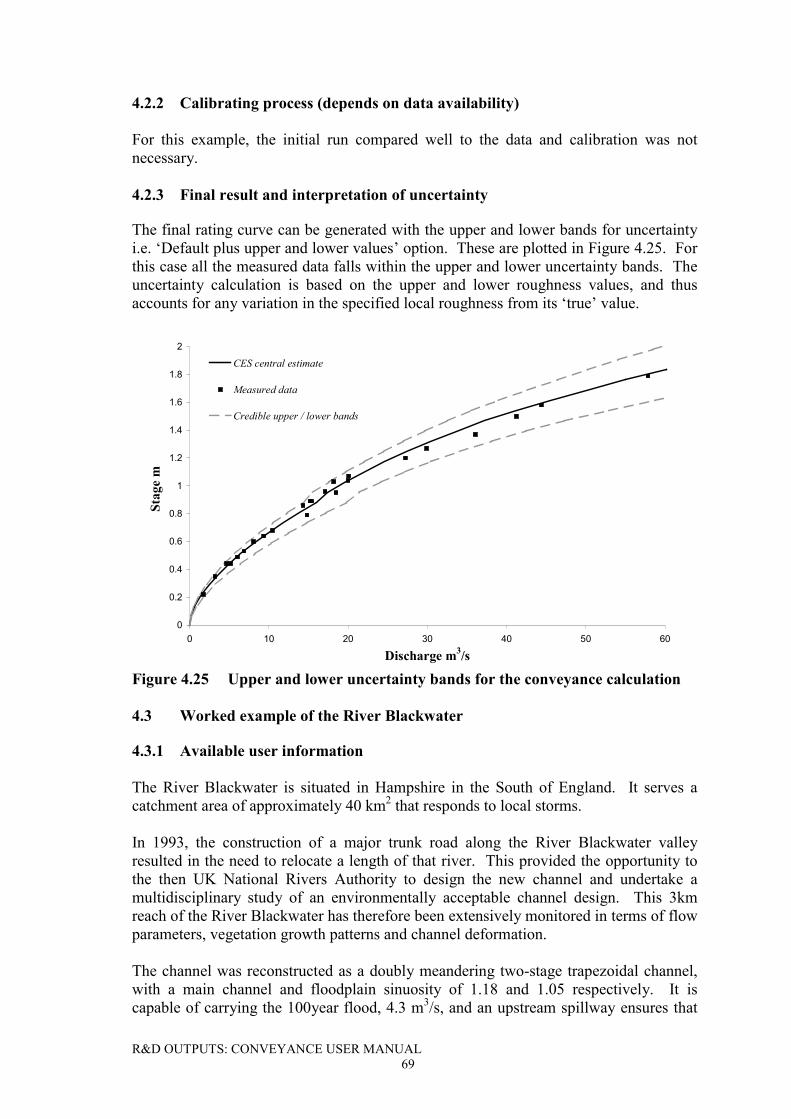
R&D OUTPUTS: CONVEYANCE USER MANUAL69
4.2.2 Calibrating process (depends on data availability)
For this example, the initial run compared well to the data and calibration was notnecessary.
4.2.3 Final result and interpretation of uncertainty
The final rating curve can be generated with the upper and lower bands for uncertaintyi.e. ‘Default plus upper and lower values’ option. These are plotted in Figure 4.25. Forthis case all the measured data falls within the upper and lower uncertainty bands. Theuncertainty calculation is based on the upper and lower roughness values, and thusaccounts for any variation in the specified local roughness from its ‘true’ value.
0
0.2
0.4
0.6
0.8
1
1.2
1.4
1.6
1.8
2
0 10 20 30 40 50 60
Discharge m3/s
Stag
e m
CES central estimate
Measured data
Credible upper / lower bands
Figure 4.25 Upper and lower uncertainty bands for the conveyance calculation
4.3 Worked example of the River Blackwater
4.3.1 Available user information
The River Blackwater is situated in Hampshire in the South of England. It serves acatchment area of approximately 40 km2 that responds to local storms.
In 1993, the construction of a major trunk road along the River Blackwater valleyresulted in the need to relocate a length of that river. This provided the opportunity tothe then UK National Rivers Authority to design the new channel and undertake amultidisciplinary study of an environmentally acceptable channel design. This 3kmreach of the River Blackwater has therefore been extensively monitored in terms of flowparameters, vegetation growth patterns and channel deformation.
The channel was reconstructed as a doubly meandering two-stage trapezoidal channel,with a main channel and floodplain sinuosity of 1.18 and 1.05 respectively. It iscapable of carrying the 100year flood, 4.3 m3/s, and an upstream spillway ensures that
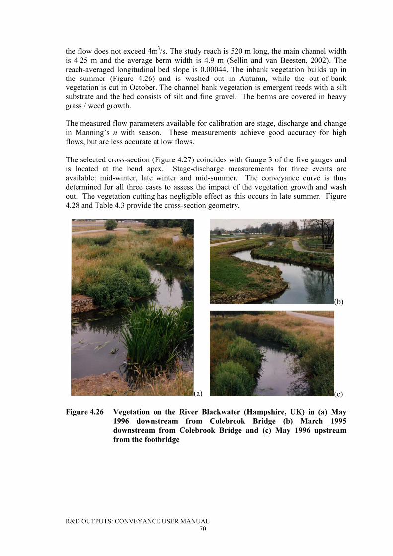
R&D OUTPUTS: CONVEYANCE USER MANUAL70
the flow does not exceed 4m3/s. The study reach is 520 m long, the main channel widthis 4.25 m and the average berm width is 4.9 m (Sellin and van Beesten, 2002). Thereach-averaged longitudinal bed slope is 0.00044. The inbank vegetation builds up inthe summer (Figure 4.26) and is washed out in Autumn, while the out-of-bankvegetation is cut in October. The channel bank vegetation is emergent reeds with a siltsubstrate and the bed consists of silt and fine gravel. The berms are covered in heavygrass / weed growth.
The measured flow parameters available for calibration are stage, discharge and changein Manning’s n with season. These measurements achieve good accuracy for highflows, but are less accurate at low flows.
The selected cross-section (Figure 4.27) coincides with Gauge 3 of the five gauges andis located at the bend apex. Stage-discharge measurements for three events areavailable: mid-winter, late winter and mid-summer. The conveyance curve is thusdetermined for all three cases to assess the impact of the vegetation growth and washout. The vegetation cutting has negligible effect as this occurs in late summer. Figure4.28 and Table 4.3 provide the cross-section geometry.
(b)
(a) (c)
Figure 4.26 Vegetation on the River Blackwater (Hampshire, UK) in (a) May1996 downstream from Colebrook Bridge (b) March 1995downstream from Colebrook Bridge and (c) May 1996 upstreamfrom the footbridge
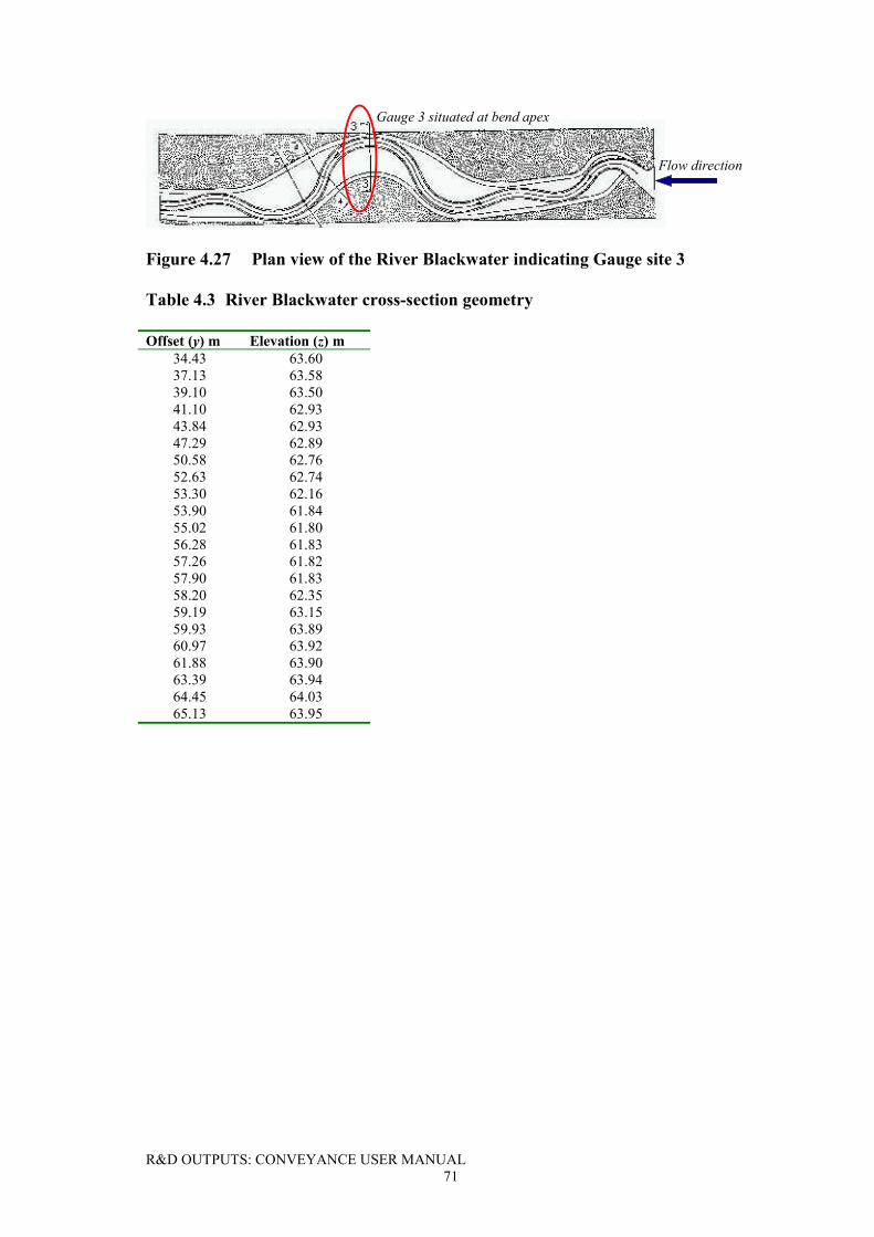
R&D OUTPUTS: CONVEYANCE USER MANUAL71
Flow direction
Gauge 3 situated at bend apex
Figure 4.27 Plan view of the River Blackwater indicating Gauge site 3
Table 4.3 River Blackwater cross-section geometry
Offset (y) m Elevation (z) m34.43 63.6037.13 63.5839.10 63.5041.10 62.9343.84 62.9347.29 62.8950.58 62.7652.63 62.7453.30 62.1653.90 61.8455.02 61.8056.28 61.8357.26 61.8257.90 61.8358.20 62.3559.19 63.1559.93 63.8960.97 63.9261.88 63.9063.39 63.9464.45 64.0365.13 63.95
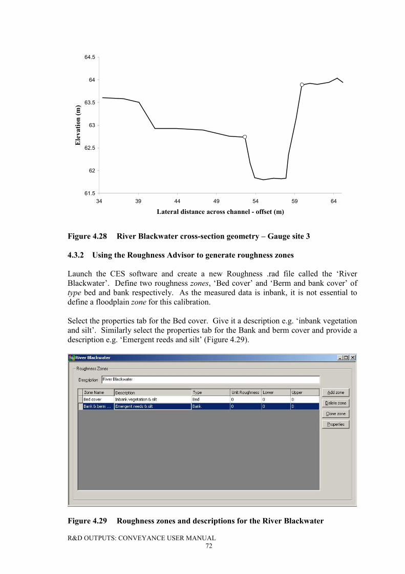
R&D OUTPUTS: CONVEYANCE USER MANUAL72
61.5
62
62.5
63
63.5
64
64.5
34 39 44 49 54 59 64
Lateral distance across channel - offset (m)
Ele
vatio
n (m
)
Figure 4.28 River Blackwater cross-section geometry – Gauge site 3
4.3.2 Using the Roughness Advisor to generate roughness zones
Launch the CES software and create a new Roughness .rad file called the ‘RiverBlackwater’. Define two roughness zones, ‘Bed cover’ and ‘Berm and bank cover’ oftype bed and bank respectively. As the measured data is inbank, it is not essential todefine a floodplain zone for this calibration.
Select the properties tab for the Bed cover. Give it a description e.g. ‘inbank vegetationand silt’. Similarly select the properties tab for the Bank and berm cover and provide adescription e.g. ‘Emergent reeds and silt’ (Figure 4.29).
Figure 4.29 Roughness zones and descriptions for the River Blackwater
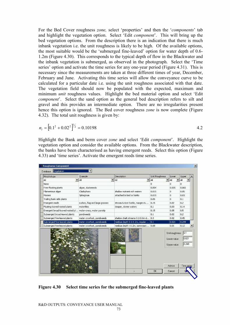
R&D OUTPUTS: CONVEYANCE USER MANUAL73
For the Bed Cover roughness zone, select ‘properties’ and then the ‘components’ taband highlight the vegetation option. Select ‘Edit component’. This will bring up thebed vegetation options. From the description there is an indication that there is muchinbank vegetation i.e. the unit roughness is likely to be high. Of the available options,the most suitable would be the ‘submerged fine-leaved’ option for water depth of 0.6-1.2m (Figure 4.30). This corresponds to the typical depth of flow in the Blackwater andthe inbank vegetation is submerged, as observed in the photograph. Select the ‘Timeseries’ option and activate the time series for any one-year period (Figure 4.31). This isnecessary since the measurements are taken at three different times of year, December,February and June. Activating this time series will allow the conveyance curve to becalculated for a particular date i.e. using the unit roughness associated with that date.The vegetation field should now be populated with the expected, maximum andminimum unit roughness values. Highlight the bed material option and select ‘Editcomponent’. Select the sand option as the general bed description refers to silt andgravel and this provides an intermediate option. There are no irregularities presenthence this option is ignored. The Bed cover roughness zone is now complete (Figure4.32). The total unit roughness is given by:
� � 10198.002.01.0 2122
���ln 4.2
Highlight the Bank and berm cover zone and select ‘Edit component’. Highlight thevegetation option and consider the available options. From the Blackwater description,the banks have been characterised as having emergent reeds. Select this option (Figure4.33) and ‘time series’. Activate the emergent reeds time series.
Figure 4.30 Select time series for the submerged fine-leaved plants
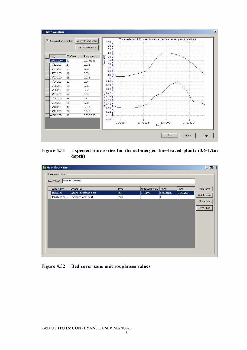
R&D OUTPUTS: CONVEYANCE USER MANUAL74
Figure 4.31 Expected time series for the submerged fine-leaved plants (0.6-1.2mdepth)
Figure 4.32 Bed cover zone unit roughness values
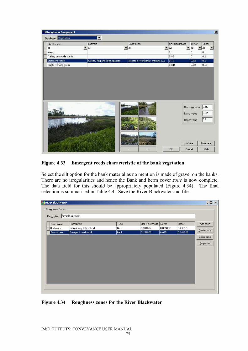
R&D OUTPUTS: CONVEYANCE USER MANUAL75
Figure 4.33 Emergent reeds characteristic of the bank vegetation
Select the silt option for the bank material as no mention is made of gravel on the banks.There are no irregularities and hence the Bank and berm cover zone is now complete.The data field for this should be appropriately populated (Figure 4.34). The finalselection is summarised in Table 4.4. Save the River Blackwater .rad file.
Figure 4.34 Roughness zones for the River Blackwater
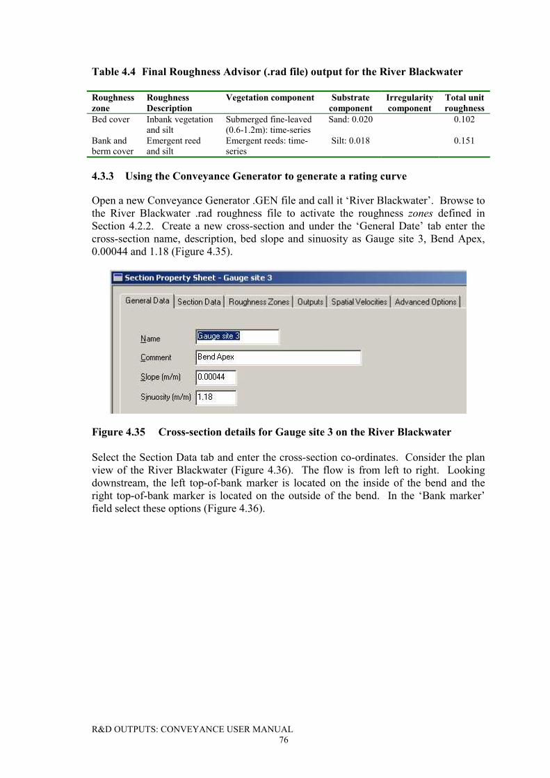
R&D OUTPUTS: CONVEYANCE USER MANUAL76
Table 4.4 Final Roughness Advisor (.rad file) output for the River Blackwater
Roughnesszone
RoughnessDescription
Vegetation component Substratecomponent
Irregularitycomponent
Total unitroughness
Bed cover Inbank vegetationand silt
Submerged fine-leaved(0.6-1.2m): time-series
Sand: 0.020 0.102
Bank andberm cover
Emergent reedand silt
Emergent reeds: time-series
Silt: 0.018 0.151
4.3.3 Using the Conveyance Generator to generate a rating curve
Open a new Conveyance Generator .GEN file and call it ‘River Blackwater’. Browse tothe River Blackwater .rad roughness file to activate the roughness zones defined inSection 4.2.2. Create a new cross-section and under the ‘General Date’ tab enter thecross-section name, description, bed slope and sinuosity as Gauge site 3, Bend Apex,0.00044 and 1.18 (Figure 4.35).
Figure 4.35 Cross-section details for Gauge site 3 on the River Blackwater
Select the Section Data tab and enter the cross-section co-ordinates. Consider the planview of the River Blackwater (Figure 4.36). The flow is from left to right. Lookingdownstream, the left top-of-bank marker is located on the inside of the bend and theright top-of-bank marker is located on the outside of the bend. In the ‘Bank marker’field select these options (Figure 4.36).
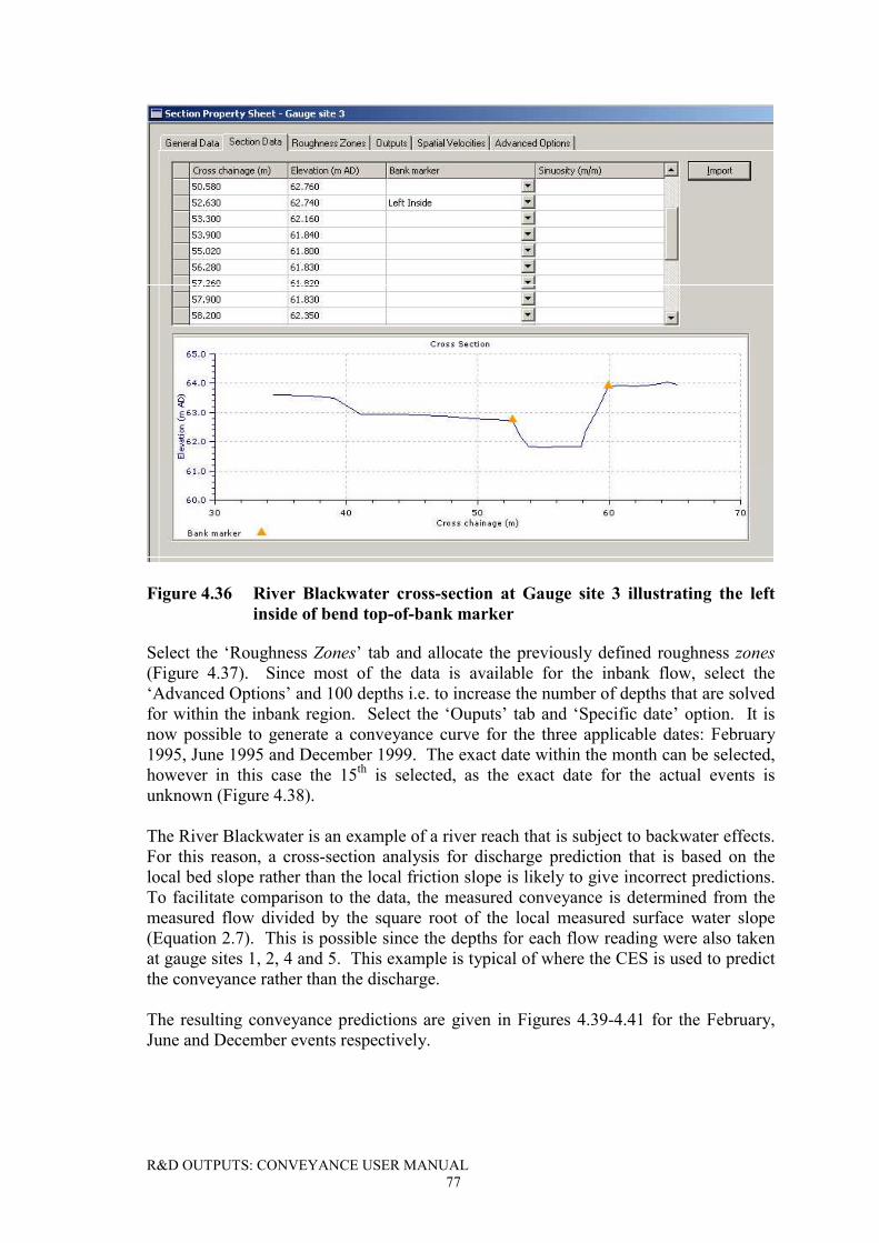
R&D OUTPUTS: CONVEYANCE USER MANUAL77
Figure 4.36 River Blackwater cross-section at Gauge site 3 illustrating the leftinside of bend top-of-bank marker
Select the ‘Roughness Zones’ tab and allocate the previously defined roughness zones(Figure 4.37). Since most of the data is available for the inbank flow, select the‘Advanced Options’ and 100 depths i.e. to increase the number of depths that are solvedfor within the inbank region. Select the ‘Ouputs’ tab and ‘Specific date’ option. It isnow possible to generate a conveyance curve for the three applicable dates: February1995, June 1995 and December 1999. The exact date within the month can be selected,however in this case the 15th is selected, as the exact date for the actual events isunknown (Figure 4.38).
The River Blackwater is an example of a river reach that is subject to backwater effects.For this reason, a cross-section analysis for discharge prediction that is based on thelocal bed slope rather than the local friction slope is likely to give incorrect predictions.To facilitate comparison to the data, the measured conveyance is determined from themeasured flow divided by the square root of the local measured surface water slope(Equation 2.7). This is possible since the depths for each flow reading were also takenat gauge sites 1, 2, 4 and 5. This example is typical of where the CES is used to predictthe conveyance rather than the discharge.
The resulting conveyance predictions are given in Figures 4.39-4.41 for the February,June and December events respectively.
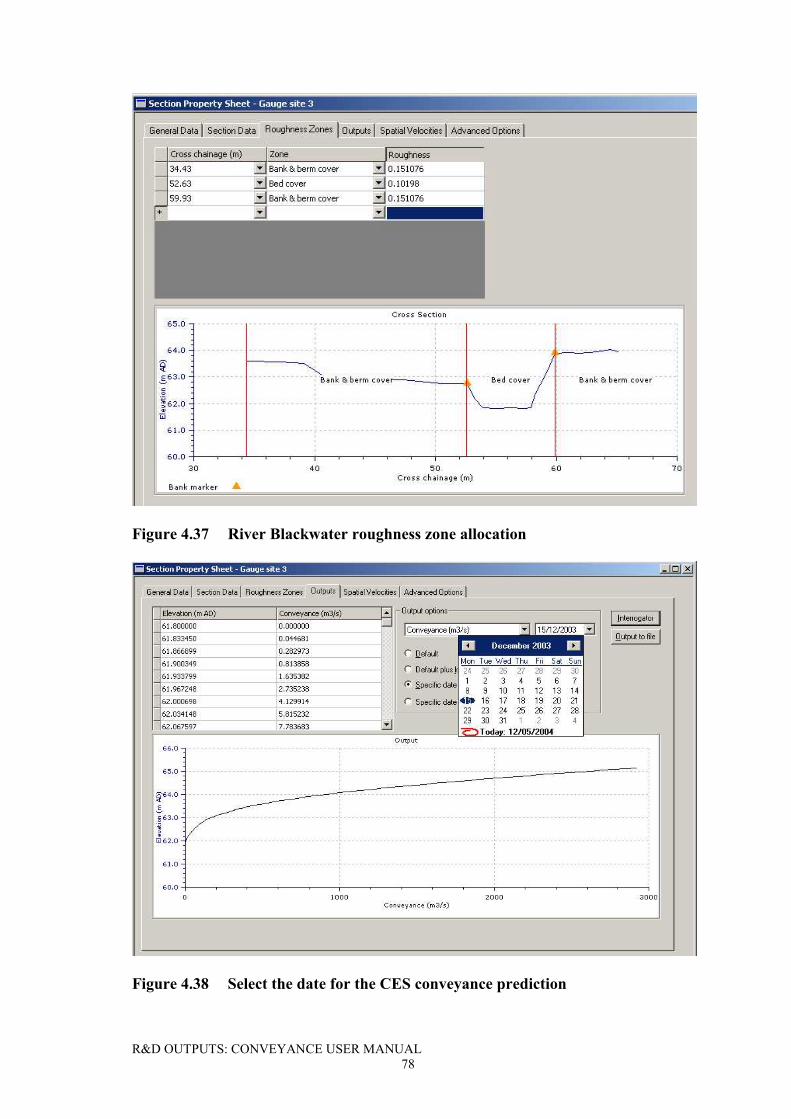
R&D OUTPUTS: CONVEYANCE USER MANUAL78
Figure 4.37 River Blackwater roughness zone allocation
Figure 4.38 Select the date for the CES conveyance prediction
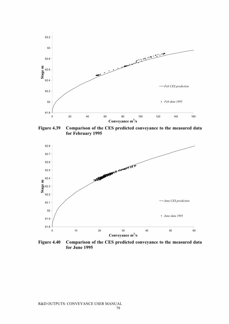
R&D OUTPUTS: CONVEYANCE USER MANUAL79
61.8
62
62.2
62.4
62.6
62.8
63
63.2
0 20 40 60 80 100 120 140 160
Conveyance m3/s
Stag
e m
Feb CES prediction
Feb data 1995
Figure 4.39 Comparison of the CES predicted conveyance to the measured datafor February 1995
61.8
61.9
62
62.1
62.2
62.3
62.4
62.5
62.6
62.7
62.8
0 10 20 30 40 50 60
Conveyance m3/s
Stag
e m
June CES prediction
June data 1995
Figure 4.40 Comparison of the CES predicted conveyance to the measured datafor June 1995
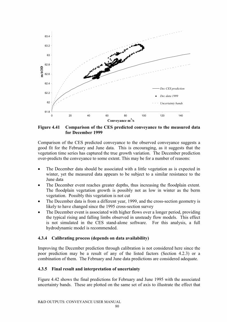
R&D OUTPUTS: CONVEYANCE USER MANUAL80
61.8
62
62.2
62.4
62.6
62.8
63
63.2
63.4
0 20 40 60 80 100 120 140
Conveyance m3/s
mA
OD
Dec CES prediction
Dec data 1999
Uncertainty bands
Figure 4.41 Comparison of the CES predicted conveyance to the measured datafor December 1999
Comparison of the CES predicted conveyance to the observed conveyance suggests agood fit for the February and June data. This is encouraging, as it suggests that thevegetation time series has captured the true growth variation. The December predictionover-predicts the conveyance to some extent. This may be for a number of reasons:
� The December data should be associated with a little vegetation as is expected inwinter, yet the measured data appears to be subject to a similar resistance to theJune data
� The December event reaches greater depths, thus increasing the floodplain extent.The floodplain vegetation growth is possibly not as low in winter as the bermvegetation. Possibly this vegetation is not cut
� The December data is from a different year, 1999, and the cross-section geometry islikely to have changed since the 1995 cross-section survey
� The December event is associated with higher flows over a longer period, providingthe typical rising and falling limbs observed in unsteady flow models. This effectis not simulated in the CES stand-alone software. For this analysis, a fullhydrodynamic model is recommended.
4.3.4 Calibrating process (depends on data availability)
Improving the December prediction through calibration is not considered here since thepoor prediction may be a result of any of the listed factors (Section 4.2.3) or acombination of them. The February and June data predictions are considered adequate.
4.3.5 Final result and interpretation of uncertainty
Figure 4.42 shows the final predictions for February and June 1995 with the associateduncertainty bands. These are plotted on the same set of axis to illustrate the effect that
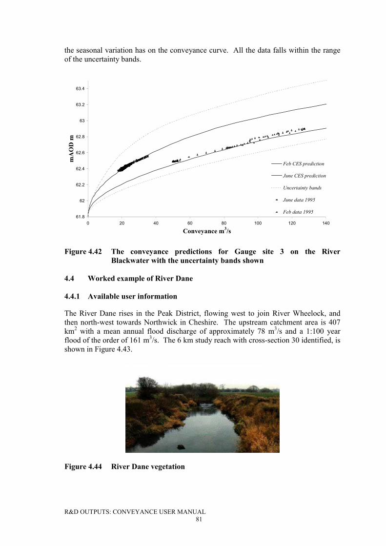
R&D OUTPUTS: CONVEYANCE USER MANUAL81
the seasonal variation has on the conveyance curve. All the data falls within the rangeof the uncertainty bands.
61.8
62
62.2
62.4
62.6
62.8
63
63.2
63.4
0 20 40 60 80 100 120 140
Conveyance m3/s
mA
OD
m
Feb CES prediction
June CES prediction
Uncertainty bands
June data 1995
Feb data 1995
Figure 4.42 The conveyance predictions for Gauge site 3 on the RiverBlackwater with the uncertainty bands shown
4.4 Worked example of River Dane
4.4.1 Available user information
The River Dane rises in the Peak District, flowing west to join River Wheelock, andthen north-west towards Northwick in Cheshire. The upstream catchment area is 407km2 with a mean annual flood discharge of approximately 78 m3/s and a 1:100 yearflood of the order of 161 m3/s. The 6 km study reach with cross-section 30 identified, isshown in Figure 4.43.
Figure 4.44 River Dane vegetation
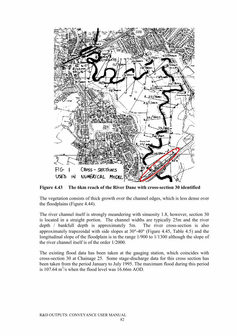
R&D OUTPUTS: CONVEYANCE USER MANUAL82
Figure 4.43 The 6km reach of the River Dane with cross-section 30 identified
The vegetation consists of thick growth over the channel edges, which is less dense overthe floodplains (Figure 4.44).
The river channel itself is strongly meandering with sinuosity 1.8, however, section 30is located in a straight portion. The channel widths are typically 25m and the riverdepth / bankfull depth is approximately 5m. The river cross-section is alsoapproximately trapezoidal with side slopes at 30�-40� (Figure 4.45, Table 4.5) and thelongitudinal slope of the floodplain is in the range 1/900 to 1/1300 although the slope ofthe river channel itself is of the order 1/2000.
The existing flood data has been taken at the gauging station, which coincides withcross-section 30 at Chainage 25. Some stage-discharge data for this cross section hasbeen taken from the period January to July 1995. The maximum flood during this periodis 107.64 m3/s when the flood level was 16.66m AOD.
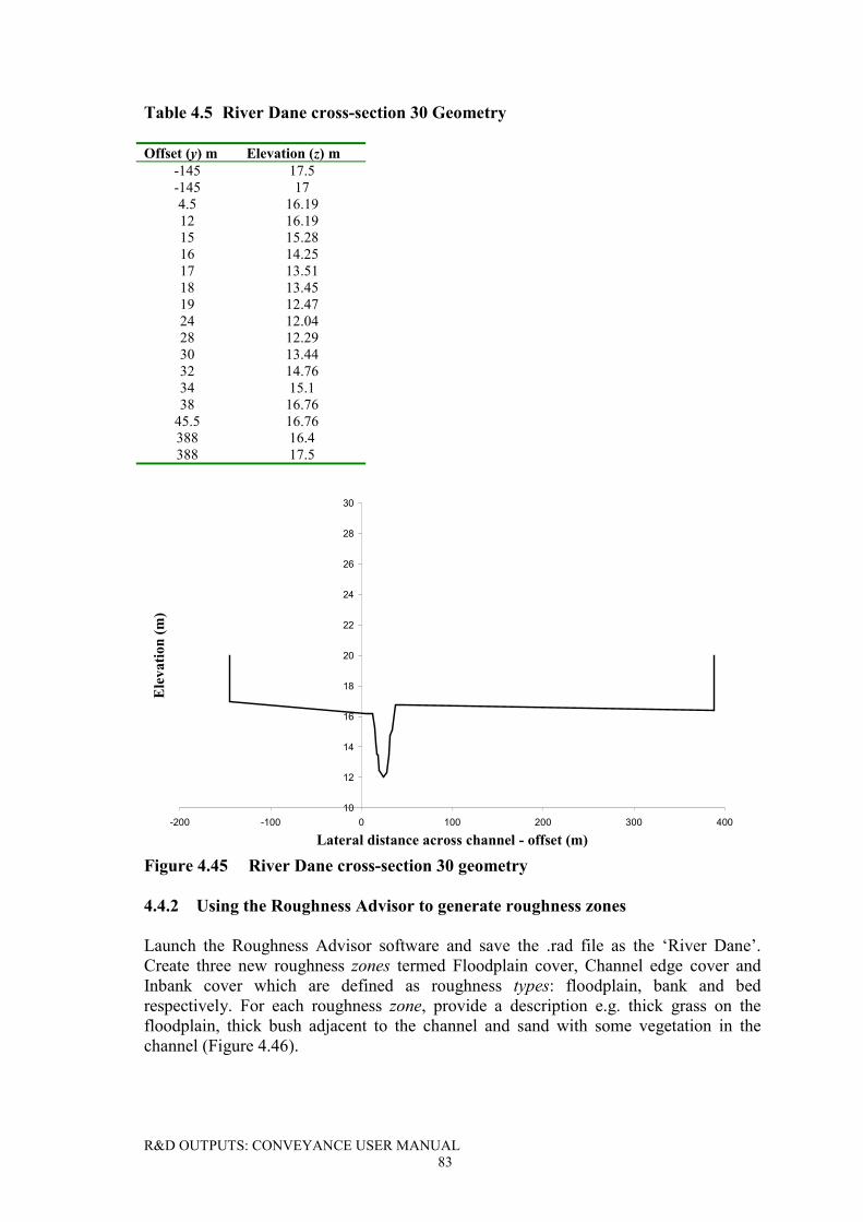
R&D OUTPUTS: CONVEYANCE USER MANUAL83
Table 4.5 River Dane cross-section 30 Geometry
Offset (y) m Elevation (z) m-145 17.5-145 174.5 16.1912 16.1915 15.2816 14.2517 13.5118 13.4519 12.4724 12.0428 12.2930 13.4432 14.7634 15.138 16.76
45.5 16.76388 16.4388 17.5
10
12
14
16
18
20
22
24
26
28
30
-200 -100 0 100 200 300 400
Lateral distance across channel - offset (m)
Ele
vatio
n (m
)
Figure 4.45 River Dane cross-section 30 geometry
4.4.2 Using the Roughness Advisor to generate roughness zones
Launch the Roughness Advisor software and save the .rad file as the ‘River Dane’.Create three new roughness zones termed Floodplain cover, Channel edge cover andInbank cover which are defined as roughness types: floodplain, bank and bedrespectively. For each roughness zone, provide a description e.g. thick grass on thefloodplain, thick bush adjacent to the channel and sand with some vegetation in thechannel (Figure 4.46).
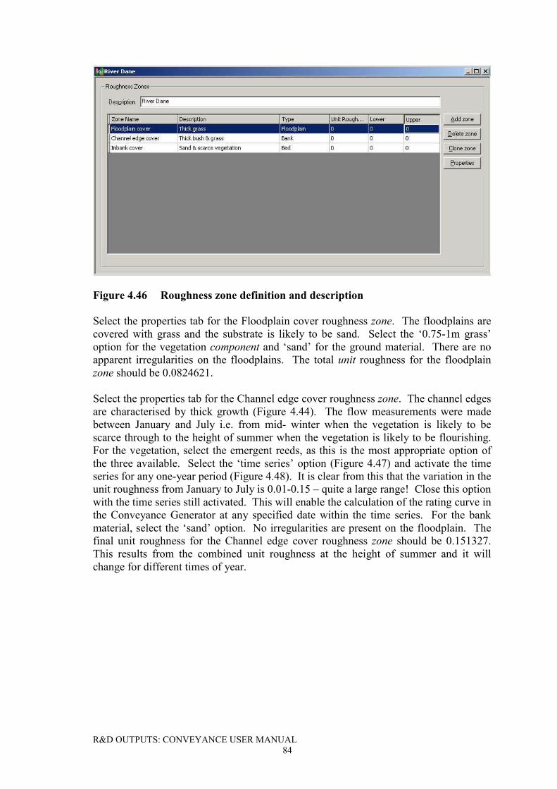
R&D OUTPUTS: CONVEYANCE USER MANUAL84
Figure 4.46 Roughness zone definition and description
Select the properties tab for the Floodplain cover roughness zone. The floodplains arecovered with grass and the substrate is likely to be sand. Select the ‘0.75-1m grass’option for the vegetation component and ‘sand’ for the ground material. There are noapparent irregularities on the floodplains. The total unit roughness for the floodplainzone should be 0.0824621.
Select the properties tab for the Channel edge cover roughness zone. The channel edgesare characterised by thick growth (Figure 4.44). The flow measurements were madebetween January and July i.e. from mid- winter when the vegetation is likely to bescarce through to the height of summer when the vegetation is likely to be flourishing.For the vegetation, select the emergent reeds, as this is the most appropriate option ofthe three available. Select the ‘time series’ option (Figure 4.47) and activate the timeseries for any one-year period (Figure 4.48). It is clear from this that the variation in theunit roughness from January to July is 0.01-0.15 – quite a large range! Close this optionwith the time series still activated. This will enable the calculation of the rating curve inthe Conveyance Generator at any specified date within the time series. For the bankmaterial, select the ‘sand’ option. No irregularities are present on the floodplain. Thefinal unit roughness for the Channel edge cover roughness zone should be 0.151327.This results from the combined unit roughness at the height of summer and it willchange for different times of year.
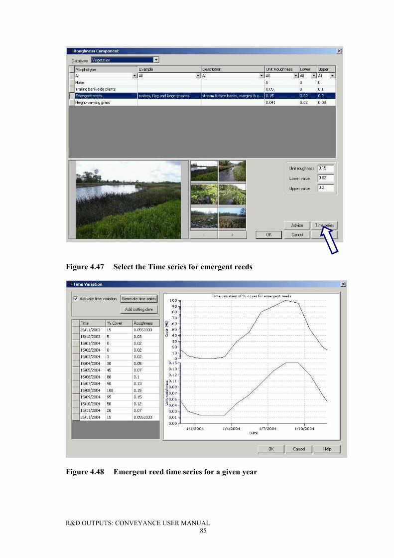
R&D OUTPUTS: CONVEYANCE USER MANUAL85
Figure 4.47 Select the Time series for emergent reeds
Figure 4.48 Emergent reed time series for a given year
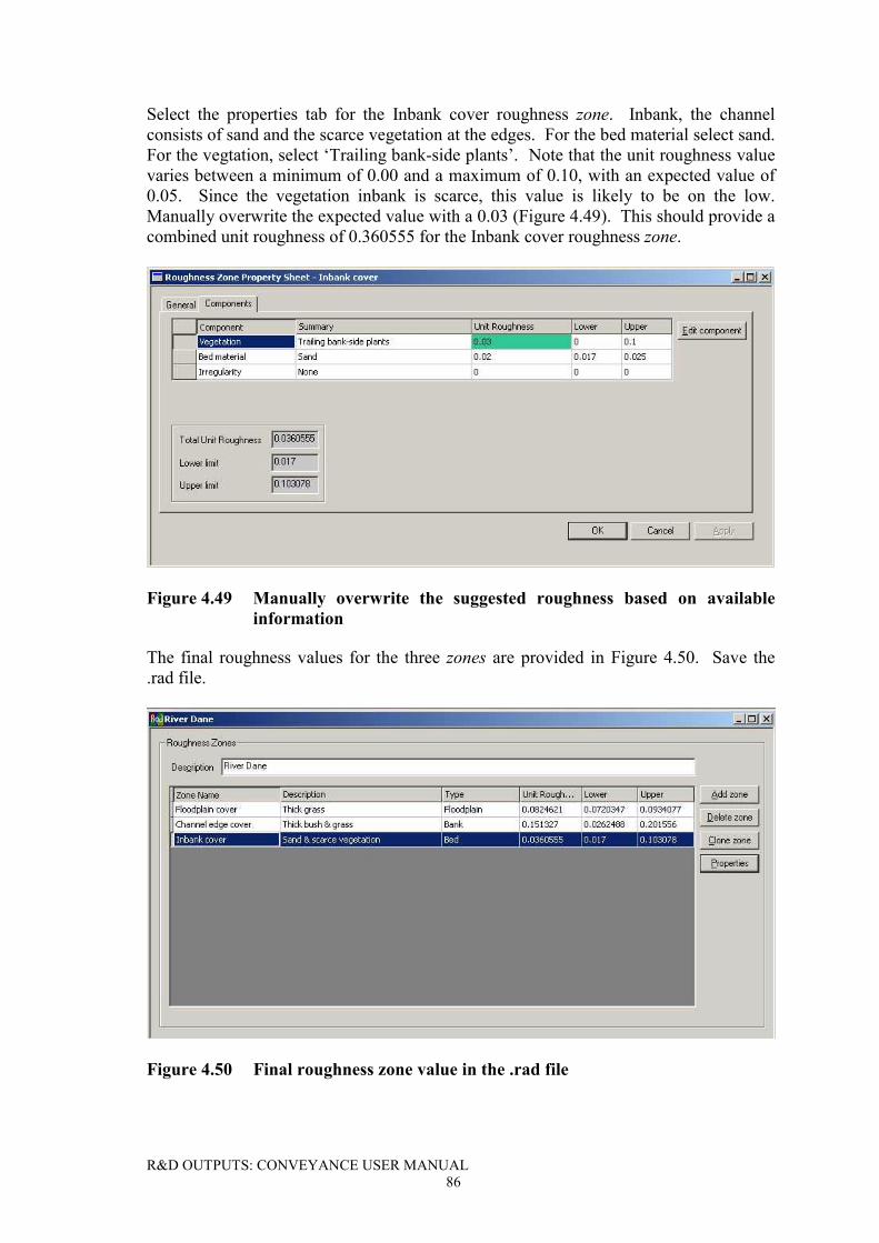
R&D OUTPUTS: CONVEYANCE USER MANUAL86
Select the properties tab for the Inbank cover roughness zone. Inbank, the channelconsists of sand and the scarce vegetation at the edges. For the bed material select sand.For the vegtation, select ‘Trailing bank-side plants’. Note that the unit roughness valuevaries between a minimum of 0.00 and a maximum of 0.10, with an expected value of0.05. Since the vegetation inbank is scarce, this value is likely to be on the low.Manually overwrite the expected value with a 0.03 (Figure 4.49). This should provide acombined unit roughness of 0.360555 for the Inbank cover roughness zone.
Figure 4.49 Manually overwrite the suggested roughness based on availableinformation
The final roughness values for the three zones are provided in Figure 4.50. Save the.rad file.
Figure 4.50 Final roughness zone value in the .rad file
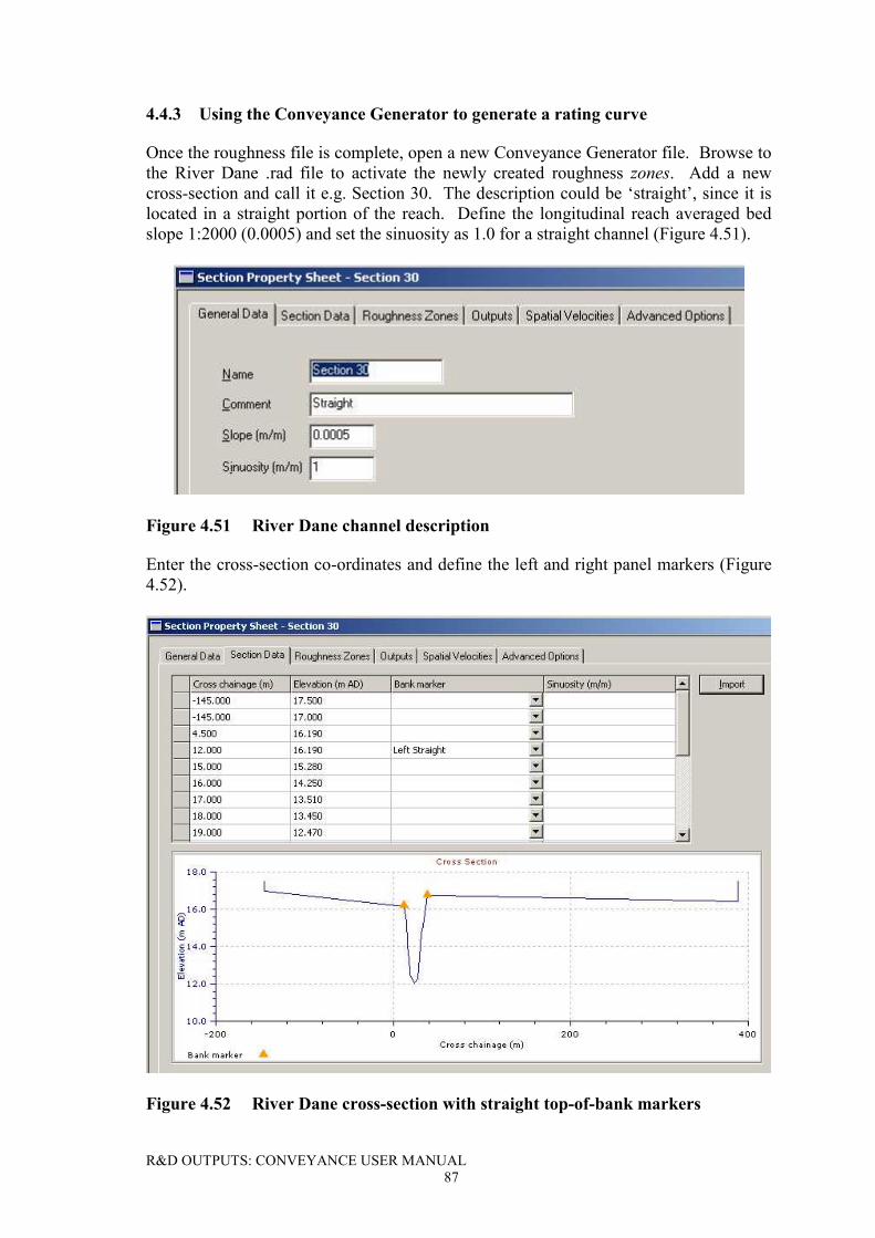
R&D OUTPUTS: CONVEYANCE USER MANUAL87
4.4.3 Using the Conveyance Generator to generate a rating curve
Once the roughness file is complete, open a new Conveyance Generator file. Browse tothe River Dane .rad file to activate the newly created roughness zones. Add a newcross-section and call it e.g. Section 30. The description could be ‘straight’, since it islocated in a straight portion of the reach. Define the longitudinal reach averaged bedslope 1:2000 (0.0005) and set the sinuosity as 1.0 for a straight channel (Figure 4.51).
Figure 4.51 River Dane channel description
Enter the cross-section co-ordinates and define the left and right panel markers (Figure4.52).
Figure 4.52 River Dane cross-section with straight top-of-bank markers
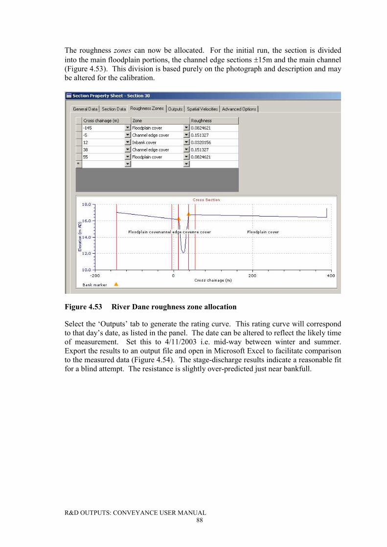
R&D OUTPUTS: CONVEYANCE USER MANUAL88
The roughness zones can now be allocated. For the initial run, the section is dividedinto the main floodplain portions, the channel edge sections �15m and the main channel(Figure 4.53). This division is based purely on the photograph and description and maybe altered for the calibration.
Figure 4.53 River Dane roughness zone allocation
Select the ‘Outputs’ tab to generate the rating curve. This rating curve will correspondto that day’s date, as listed in the panel. The date can be altered to reflect the likely timeof measurement. Set this to 4/11/2003 i.e. mid-way between winter and summer.Export the results to an output file and open in Microsoft Excel to facilitate comparisonto the measured data (Figure 4.54). The stage-discharge results indicate a reasonable fitfor a blind attempt. The resistance is slightly over-predicted just near bankfull.
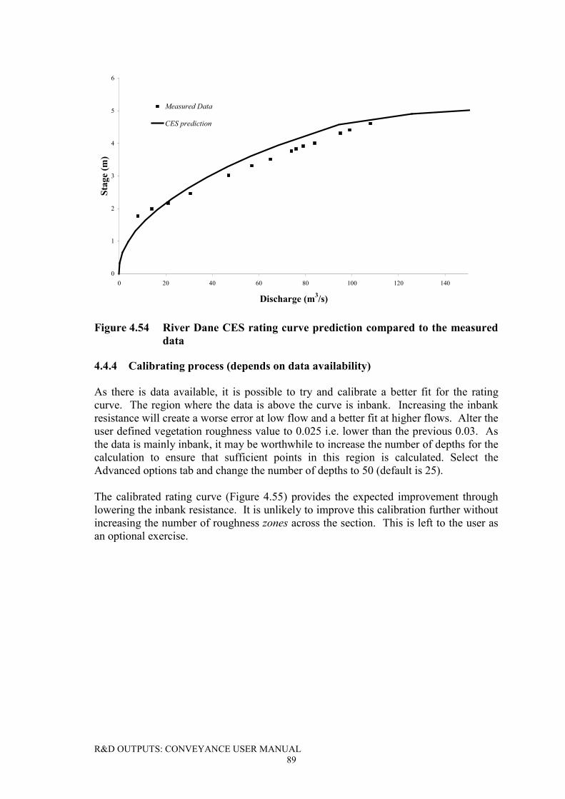
R&D OUTPUTS: CONVEYANCE USER MANUAL89
0
1
2
3
4
5
6
0 20 40 60 80 100 120 140
Discharge (m3/s)
Stag
e (m
)Measured Data
CES prediction
Figure 4.54 River Dane CES rating curve prediction compared to the measureddata
4.4.4 Calibrating process (depends on data availability)
As there is data available, it is possible to try and calibrate a better fit for the ratingcurve. The region where the data is above the curve is inbank. Increasing the inbankresistance will create a worse error at low flow and a better fit at higher flows. Alter theuser defined vegetation roughness value to 0.025 i.e. lower than the previous 0.03. Asthe data is mainly inbank, it may be worthwhile to increase the number of depths for thecalculation to ensure that sufficient points in this region is calculated. Select theAdvanced options tab and change the number of depths to 50 (default is 25).
The calibrated rating curve (Figure 4.55) provides the expected improvement throughlowering the inbank resistance. It is unlikely to improve this calibration further withoutincreasing the number of roughness zones across the section. This is left to the user asan optional exercise.
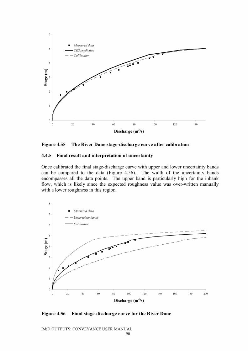
R&D OUTPUTS: CONVEYANCE USER MANUAL90
0
1
2
3
4
5
6
0 20 40 60 80 100 120 140
Discharge (m3/s)
Stag
e (m
)Measured dataCES predictionCalibration
Figure 4.55 The River Dane stage-discharge curve after calibration
4.4.5 Final result and interpretation of uncertainty
Once calibrated the final stage-discharge curve with upper and lower uncertainty bandscan be compared to the data (Figure 4.56). The width of the uncertainty bandsencompasses all the data points. The upper band is particularly high for the inbankflow, which is likely since the expected roughness value was over-written manuallywith a lower roughness in this region.
0
1
2
3
4
5
6
7
8
0 20 40 60 80 100 120 140 160 180 200
Discharge (m3/s)
Stag
e (m
)
Measured data
Uncertainty bands
Calibrated
Figure 4.56 Final stage-discharge curve for the River Dane
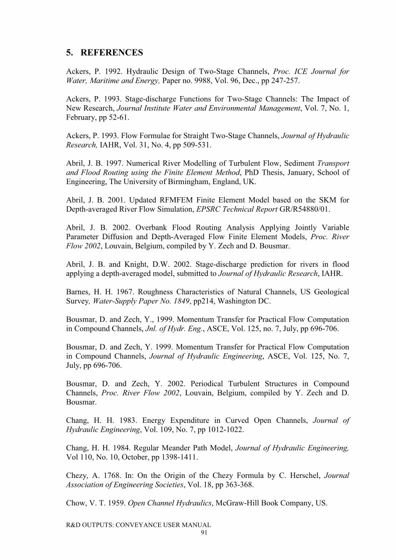
R&D OUTPUTS: CONVEYANCE USER MANUAL91
5. REFERENCES
Ackers, P. 1992. Hydraulic Design of Two-Stage Channels, Proc. ICE Journal forWater, Maritime and Energy, Paper no. 9988, Vol. 96, Dec., pp 247-257.
Ackers, P. 1993. Stage-discharge Functions for Two-Stage Channels: The Impact ofNew Research, Journal Institute Water and Environmental Management, Vol. 7, No. 1,February, pp 52-61.
Ackers, P. 1993. Flow Formulae for Straight Two-Stage Channels, Journal of HydraulicResearch, IAHR, Vol. 31, No. 4, pp 509-531.
Abril, J. B. 1997. Numerical River Modelling of Turbulent Flow, Sediment Transportand Flood Routing using the Finite Element Method, PhD Thesis, January, School ofEngineering, The University of Birmingham, England, UK.
Abril, J. B. 2001. Updated RFMFEM Finite Element Model based on the SKM forDepth-averaged River Flow Simulation, EPSRC Technical Report GR/R54880/01.
Abril, J. B. 2002. Overbank Flood Routing Analysis Applying Jointly VariableParameter Diffusion and Depth-Averaged Flow Finite Element Models, Proc. RiverFlow 2002, Louvain, Belgium, compiled by Y. Zech and D. Bousmar.
Abril, J. B. and Knight, D.W. 2002. Stage-discharge prediction for rivers in floodapplying a depth-averaged model, submitted to Journal of Hydraulic Research, IAHR.
Barnes, H. H. 1967. Roughness Characteristics of Natural Channels, US GeologicalSurvey, Water-Supply Paper No. 1849, pp214, Washington DC.
Bousmar, D. and Zech, Y., 1999. Momentum Transfer for Practical Flow Computationin Compound Channels, Jnl. of Hydr. Eng., ASCE, Vol. 125, no. 7, July, pp 696-706.
Bousmar, D. and Zech, Y. 1999. Momentum Transfer for Practical Flow Computationin Compound Channels, Journal of Hydraulic Engineering, ASCE, Vol. 125, No. 7,July, pp 696-706.
Bousmar, D. and Zech, Y. 2002. Periodical Turbulent Structures in CompoundChannels, Proc. River Flow 2002, Louvain, Belgium, compiled by Y. Zech and D.Bousmar.
Chang, H. H. 1983. Energy Expenditure in Curved Open Channels, Journal ofHydraulic Engineering, Vol. 109, No. 7, pp 1012-1022.
Chang, H. H. 1984. Regular Meander Path Model, Journal of Hydraulic Engineering,Vol 110, No. 10, October, pp 1398-1411.
Chezy, A. 1768. In: On the Origin of the Chezy Formula by C. Herschel, JournalAssociation of Engineering Societies, Vol. 18, pp 363-368.
Chow, V. T. 1959. Open Channel Hydraulics, McGraw-Hill Book Company, US.
R&D OUTPUTS: CONVEYANCE USER MANUAL92
Colebrook, C. F. and White, C. M. 1937. Experiments with Fluid Friction in RoughenedPipes, Proc. of the Royal Society, A161, pp 367-379.
Cowan, W. L. 1956. Estimating Hydraulic Roughness Coefficients, AgriculturalEngineering, Vol. 37, pp 473-475.
DEFRA/EA, 2002. Reducing Uncertainty in River Flood Conveyance, Interim Report 1:Data Mining, Project W5A- 057, HR Wallingford Ltd., United Kingdom.
DEFRA/EA, 2003a. Reducing Uncertainty in River Flood Conveyance, Interim Report2: Review of Methods for Estimating Conveyance, Project W5A- 057, HR WallingfordLtd., United Kingdom.
DEFRA/EA, 2003b. Reducing Uncertainty in River Flood Conveyance, RoughnessReview, Project W5A- 057, HR Wallingford Ltd., United Kingdom.
DEFRA/EA, 2004/5. Reducing Uncertainty in River Flood Conveyance, Interim Report3: Testing of Conveyance Methods in 1D River Models, Project W5A- 057,HR Wallingford Ltd., United Kingdom.
Einstein, H. A. and Banks, R. B. 1950. Fluid Resistance of Composite Roughness,Transactions of the American Geophysical Union, Volume 31, No. 4, pp 603-610.
Evans, E. P., Pender, G., Samuels, P. G. and Escarameia, M. 2001. ReducingUncertainty in River Flood Conveyance: Scoping Study, R&D Technical Report toDEFRA / Environment Agency, Project W5A- 057, HR Wallingford Ltd., UnitedKingdom.
Ervine, D. A. and Ellis, J. 1987. Experimental and Computational Aspects of OverbankFloodplain Flow, Trans. Royal Society of Edinburgh: Earth Sciences, Vol. 78, pp 315–475.
Ervine, D. A., Babaeyan-Koopaei, K. and Sellin, H.J. 2000. Two-dimensional Solutionfor Straight and Meandering Overbank Flows, Journal of Hydraulic Engineering,ASCE, Vol. 126, no. 9, September, pp 653-669.
Hicks, D. M. and Mason, P. D. 1998. Roughness Characteristics of New ZealandRivers, NIWA, Christchurch, 329pp.
HR Wallingford, 2002. Risk Performance and Uncertainty in Flood and CoastalDefence - A Review. Report SR 587 (Second Draft). HR Wallingford.
Intergovernmental Panel on Climate Change (2001). Climate Change 2001, Impacts,Adaptation and Vulnerability, Cambridge University Press.
James, C. S. and Wark, J. B. 1992. Conveyance Estimation for Meandering Channels,HR Wallingford Ltd. Report SR 329, pp 1-91.
R&D OUTPUTS: CONVEYANCE USER MANUAL93
Knight, D. W., 1981. Some field measurements concerned with the behaviour ofresistance coefficients in a tidal channel, Estuarine, Coastal and Shelf Science, Vol. 12,pp 303-322.
Knight, D. W. and Abril, B. J. 1996. Refined Calibration of a Depth-Averaged Modelfor Turbulent Flow in a Compound Channel, Proc. Inst. of Civil Engineers Water,Maritime and Energy, Paper 11017, Vol. 118, Sept., pp 151-159.
Manning, R. 1890. On the Flow of Water in Open Channels and Pipes, Transactions ofthe Institute of Civil Engineers of Ireland, Vol. 20, pp 161-207.
National Research Council (NRC). 2000. Risk Analysis and Uncertainty in FloodDamage Reduction Studies. Washington, D.C.: National Academy Press.
Nikuradse, J. 1933. Translates to: Laws of Flow in Rough Pipes, Verein deutscherIngenieure, Forschubgsheft, No. 361, Berlin.
Raven, P. J., Holmes, H. T. H., Dawson, F.H., Fox, P. J. A., Everard, M., Fozzard, I.and Rouen K. J. 1998. River Habitat Quality The Physical Character of Rivers andStreams in the UK and the Isle of Man, River Habitat Report No. 2, EnvironmentAgency, pp 90.
Raudkivi, A. J. 1998. Loose Boundary Hydraulics, A.A. Balkema, Rotterdam,Netherlands.
Samuels, P. G. 1985. Modelling of River and Flood Plain Flow using the Finite ElementMethod, PhD Thesis, Department of Mathematics, University of Reading, HydraulicsResearch Report no. SR61, November.
Samuels, P. G. 1988. Lateral Shear Layers in Compound Channels, InternationalConference on Fluvial Hydraulics.
Samuels, P. G. 1989. The hydraulics of Two-stage Channels – Review of CurrentKnowledge, Conference of River Engineers, University of Loughborough, HRPublished Paper no. 45.
Samuels, P. G. 1989. Some Analytical Aspects of Depth Averaged Flow Models, Intnl.Conf. Hydraulic and Environmental Modelling of Coastal, Estuarine and River Waters,Bradford, England, 19-21 September.
Samuels, P. G. 1989. Backwater lengths in rivers, Proc. Inst. of Civil Engineers, Part 2,Vol. 87, pp 571-582.
Samuels, P. G. 1995. Uncertainty in Flood Level Prediction, XXVI Biannual Congressof the IAHR, HYDRA2000, London, Sept 1995, Volume 1 of Proceedings published byThomas Telford.
Samuels, P. G., Bramley, M. E. and Evans, E. P. 2002. Reducing Uncertainty inConveyance Estimation, Paper presented at River Flow 2002, Université CatholiqueLouvain, September 2002, Papers published by Balkema & Sons.
R&D OUTPUTS: CONVEYANCE USER MANUAL94
Sellin, R. H. J. and van Beesten, D. P. 2002. Berm Vegetation and its Effect on FlowResistance in a Two-Stage River Channel: An Analysis of Field Data, Proceedings ofthe River Flow 2002 Conference, Belgium, Zwets and Zeitlinger, Lisse, ISBN 90 5809509 6, Volume 1, pp 319-327.
Shiono, K. and Knight, D. W. 1989. Two-Dimensional Analytical Solution forCompound Channel, Proc. 3rd Intl. Symposium on Refined Flow Modelling andTurbulence Measurements, Universal Academy Press, pp 591-599.
Shiono, K. and Knight, D. W. 1991. Turbulent Open-channel flows with Variable Depthacross the Section, Journal of Fluid Mechanics, Vol. 222, pp 617-646.
Shiono, K. and Knight, D. W. 1990. Mathematical Models of Flow in Two or MultiStage Straight Channels, International Conference on River Flood Hydraulics, (Ed.W.R.White), Wiley and sons Ltd., Paper G1, pp229-238.
Shiono, K. and Muto, Y. 1998. Complex Flow Mechanisms in Compound MeanderingChannels with Overbank Flow, Journal of Fluid Mechanics, Vol 376, pp 221-261.
Shiono, K., Muto, Y., Knight, D. W. and Hyde, A. F. L. 1999. Energy Losses due toSecondary Flow and Turbulence in Meandering Channels with Overbank Flow, Journalof Hydraulic Research, IAHR, Vol. 37, No. 5, pp 641-664.