Loughborough UniversityInstitutional Repository

Degradation mechanisms ofbioresorbable polyesters.Part 1, Effects of randomscission, end scission and

autocatalysis

This item was submitted to Loughborough University's Institutional Repositoryby the/an author.

Citation: GLEADALL, A. ... et al., 2014. Degradation mechanisms of biore-sorbable polyesters. Part 1, Effects of random scission, end scission and auto-catalysis. Acta Biomaterialia, 10 (5), pp.2223-2232.

Metadata Record: https://dspace.lboro.ac.uk/2134/26775

Version: Accepted for publication

Publisher: Elsevier ( c© Acta Materialia Inc.)

Rights: This work is made available according to the conditions of the Cre-ative Commons Attribution-NonCommercial-NoDerivatives 4.0 International(CC BY-NC-ND 4.0) licence. Full details of this licence are available at:https://creativecommons.org/licenses/by-nc-nd/4.0/

Please cite the published version.

1

Degradation mechanisms of bioresorbable polyesters. Part 1. Effects of

random scission, end scission and autocatalysis

Andrew Gleadalla, Jingzhe Pan*a, and Marc-Anton Kruftb

a Department of Engineering, University of Leicester, Leicester, LE1 7RH, UK

b Purac Biomaterials, P.O. Box 21, 4200 AA Gorinchem, The Netherlands

* Corresponding author. Tel: +44 (0)116 223 1092; Fax: +44 (0)116 252 2525; E-mail:

jp165@le.ac.uk;

The final publication is available at Elsevier via http://dx.doi.org/10.1016/j.actbio.2013.12.039

ABSTRACT: A mathematical model was developed to relate the degradation trend of

bioresorbable polymers to different underlying hydrolysis mechanisms including noncatalytic

random scission, autocatalytic random scission, noncatalytic end scission or autocatalytic end

scission. The effect of each mechanism on molecular weight degradation and potential mass

loss was analysed. A simple scheme was developed to identify the most likely hydrolysis

mechanism based on experimental data. The scheme was firstly demonstrated using case

studies and then used to evaluate data collected from 31 publications in the literature to identify

the dominant hydrolysis mechanisms for typical biodegradable polymers. The analysis showed

that most of the experimental data indicates autocatalytic hydrolysis as expected. However the

study shows that the existing understanding on whether random or end scission controls

degradation is inappropriate. It was revealed that pure end scission cannot explain the observed

trend in molecular weight reduction because it would be too slow for end scission to reduce the

average molecular weight. On the other hand pure random scission cannot explain the observed

trend in mass loss because too few oligomers would be available to diffuse out of a device. It

is concluded that the chain ends are more susceptible to cleavage which produces most of the

oligomers leading to mass loss. However it is random scission that dominates the reduction in

molecular weight.

Key words: Biodegradable polymers, biodegradation, random scission, end scission,

modelling.

2

1. Introduction

A large number of experiments have been conducted to understand the degradation of

bioresorbable polymers such as polylactic acid (PLA), polyglycolic acid (PGA) and

polycaprolactone (PCL) [1-31] which are used for various medical applications. A

phenomenological mathematical model has been developed by Pan and his co-workers to

predict the degradation rate of the biodegradable polymers [32-35]. It was demonstrated that

the model is able to fit a wide range of experimental data for changes in molecular weight,

mass and crystallinity as functions of degradation time. The purpose of this paper is to present

a more detailed model that can be used to relate degradation behaviour to the underlying

hydrolysis mechanisms. The mathematical model is used in order to understand the

fundamental effects of each hydrolysis mechanism. It is not proposed to be able to predict

degradation characteristics from initial material properties because the effects of many factors

are not currently understood in enough detail.

The hydrolysis mechanisms being considered include random scission, end scission,

noncatalytic hydrolysis and autocatalytic hydrolysis. In noncatalytic degradation, the ester

bonds are cleaved in the presence of water whereas for autocatalytic degradation the hydrolysis

reaction are catalysed by the carboxylic acid chain ends of water-soluble oligomers and

monomers [1]. In random scission it is assumed that each ester bond in the polymer has an

equal chance of chain cleavage whereas end scission assumes that only ester bonds at the end

of polymer chains are cleaved. Experimental evidence for which hydrolysis mechanisms are

dominant is conflicting due to the number of factors that affect degradation and inconsistency

between experiments. Shih [36] suggested that end scission is dominant with approximately 10

times the rate of random scission. However for a high molecular weight sample, a single

random scission has a greater impact on molecular weight than 1000 end scissions so their

experiment actually indicates that random scission controls the molecular weight reduction.

The experiment by Schliecker et al. [13] supports the theory of noncatalytic hydrolysis because

it was found that the addition of oligomers does not accelerate degradation. Other experiments

support the theory of autocatalytic hydrolysis [2, 37]. It has been widely observed that

degradation occurs faster at the core of large samples compared to the surface because

oligomers and monomers, which act as catalysts, diffuse out of the polymer near the surface

[22]. Currently, there is no simple method of interpreting experimental data to identify the

underlying hydrolysis mechanisms.

It has been suggested that a linear relationship between (1/Mn) and time indicates noncatalytic

hydrolysis [38] and a linear relationship between (1/Mn)0.5 and time indicates autocatalytic

3

hydrolysis [1, 37]. However, there is considerable experimental data in that literature that

demonstrates a delay before the reduction of molecular weight [10, 22-29], and therefore does

not fit either trend. The experiments of Antheunis et al. [27] demonstrate a delay trend when

initial polymer chains do not possess carboxylic acid end groups but no delay when they do.

The model here considers hydrolysis to only be catalysed by the acid chain ends of water

soluble oligomers and monomers, not the chain ends of long chains which may be unable to

catalyse hydrolysis due to lack of mobility or may initially not possess carboxylic acid end

groups. One purpose of the current paper is to provide a wider interpretation of autocatalytic

hydrolysis.

It is not fully understood which hydrolysis mechanisms are generally most prevalent in

degradation experiments. In this paper, an analysis scheme is developed that can quickly

identify which hydrolysis mechanisms are likely to be dominant based on experimental data

for molecular weight and/or mass loss. The trends of molecular weight degradation and mass

loss predicted by the mathematical model for various combinations of

noncatalytic/autocatalytic hydrolysis and random/end scission are analysed and translated into

the simple analysis scheme. Case studies demonstrate the use of the scheme and a large set of

experimental data from the literature is evaluated to identify the dominant hydrolysis

mechanisms. The particular focus of this study is predominantly on poly(lactide) and

poly(glycolide) polymers in order to draw unambiguous conclusions regarding their

degradation. However, the qualitative analysis scheme is not constrained to just poly(lactide)

and poly(glycolide). The effects of initial molecular weight and residual monomer in relation

to the hydrolysis mechanism are the subject of a separate paper [39].

2. The mathematical model

The phenomenological model developed by Pan and co-workers [32-34] is modified to separate

the different hydrolysis mechanisms including noncatalytic random scission, autocatalytic

random scission, noncatalytic end scission and autocatalytic end scission. The polymer is

assumed to consist of amorphous polymer chains, oligomers, monomers and a crystalline

phase. It is assumed that the crystalline phase, characterised by the degree of crystallinity Xc

(no units) strongly resists hydrolysis such that only the amorphous polymer chains suffer from

hydrolysis chain scission. The rate of chain scission is determined by the concentrations of the

reactants and catalyst. For random scission, the reactant is the ester bonds in amorphous chains

which are characterised by the concentration Ce (mol m-3). For end scission the reactant is the

amorphous chain ends characterised by Cend (mol m-3). It is assumed that water is always

4

abundant [40] and its concentration does not affect the hydrolysis rate. The hydrolysis reaction

can be catalysed by H+ disassociated from the carboxylic acid end groups. Using Cacid (mol m-

3) to represent the concentration of the carboxylic end groups, the concentration of H+ can be

calculated as [34] where Ka is the acid disassociation constant and n (no units)

is taken to be 0.5 as suggested by Siparsky et al. [37] indicating equilibrium condition for acid

disassociation. We use Rrs (mol m-3) and Res (mol m-3) to represent the molar concentrations

for random and end scissions respectively. Following Han et al. [34] the rate of random scission

is given by

(1)

and the rate of end scission is given by

.

(2)

Here kr1 and ke1 (day-1) are the noncatalytic reaction constants and kr2 and ke2 ([mol-1m3]0.5day-

1) are the autocatalytic reaction constants where subscripts r and e indicate random and end

scission respectively. The acid disassociation constant Ka has been merged into kr2 and ke2. The

single rate equation for chain scission proposed by Han et al. [34] has been split into two

equations so that the random and end scissions can be evaluated separately. The total scission

concentration Rs (mol m-3) is then given by

. (3)

In end scission a monomer is produced by each scission and the production of monomers per

unit volume Rm (mol m-3) is simply given by

Rm = Res . (4)

In random scission an oligomer may be produced by chance if an ester bond near a chain end

is cleaved. Following the statistical analysis by Flory [41] the production of ester units of

oligomers per unit volume, Rol (mol m-3), can be related to the concentration of random

scissions Rrs through

(5)

in which Ce0 (mol m-3) is the concentration of ester bonds in all phases at time t = 0. The values

α = 28 (no units) and β = 2 (no units) apply if the oligomers are defined as short chains of less

than 8 units [38] as assumed in this work.

nacidaHCKC

n

c

aciderer

rs

X

CCkCk

dt

dR

121

n

c

acidendeende

es

X

CCkCk

dt

dR

121

esrss RRR

00 e

rs

e

ol

C

R

C

R

5

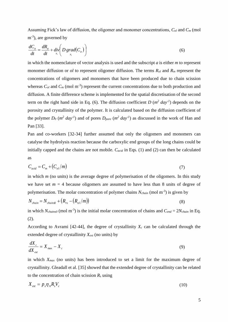
Assuming Fick’s law of diffusion, the oligomer and monomer concentrations, Col and Cm (mol

m-3), are governed by

(6)

in which the nomenclature of vector analysis is used and the subscript a is either m to represent

monomer diffusion or ol to represent oligomer diffusion. The terms Rol and Rm represent the

concentrations of oligomers and monomers that have been produced due to chain scission

whereas Col and Cm (mol m-3) represent the current concentrations due to both production and

diffusion. A finite difference scheme is implemented for the spatial discretisation of the second

term on the right hand side in Eq. (6). The diffusion coefficient D (m2 day-1) depends on the

porosity and crystallinity of the polymer. It is calculated based on the diffusion coefficient of

the polymer D0 (m2 day-1) and of pores Dpore (m

2 day-1) as discussed in the work of Han and

Pan [33].

Pan and co-workers [32-34] further assumed that only the oligomers and monomers can

catalyse the hydrolysis reaction because the carboxylic end groups of the long chains could be

initially capped and the chains are not mobile. Cacid in Eqs. (1) and (2) can then be calculated

as

(7)

in which m (no units) is the average degree of polymerisation of the oligomers. In this study

we have set m = 4 because oligomers are assumed to have less than 8 units of degree of

polymerisation. The molar concentration of polymer chains Nchain (mol m-3) is given by

(8)

in which Nchains0 (mol m-3) is the initial molar concentration of chains and Cend = 2Nchain in Eq.

(2).

According to Avrami [42-44], the degree of crystallinity Xc can be calculated through the

extended degree of crystallinity Xext (no units) by

(9)

in which Xmax (no units) has been introduced to set a limit for the maximum degree of

crystallinity. Gleadall et al. [35] showed that the extended degree of crystallinity can be related

to the concentration of chain scission Rs using

(10)

a

xx

aa CgradDdivdt

dR

dt

dC

ii

mCCC olmacid

mRRNN olrschainschain 0

c

ext

c XXdX

dX max

csAxext VRpX

6

in which px (no units) is the probability of crystallisation of a cleaved chain, ηA is Avogadro’s

constant (mol-1), Vc (m3) is the volume of a single polymer crystallite. During biodegradation

amorphous polymer chains are consumed by oligomer production, monomer production and

crystallisation which leads to

(11)

where ω (no units) is the inverse molar volume of crystalline phase.

The number-averaged molecular weight, Mn (g mol-1), can be calculated as

(12)

in which M0 (g mol-1) is the molar mass of each polymer repeat unit. In the molecular weight

calculation, oligomers and monomers are excluded because they are too small to be detected

by typical measuring techniques such as gel permeation chromatography. Each random

scission increases the chain number by one but has a probability to produce Rol / m number of

oligomers. For end scission, Nchain remains constant and Mn reduces due to the reduction of

amorphous ester units Ce. In contrast, for random scission, the main factor for Mn reduction is

the increase in the number of chains.

Eqs. (1 – 12) are numerically integrated using the direct Euler scheme giving the molecular

weight, degree of crystallinity, and concentrations of oligomers and monomers as functions of

degradation time. Although there are a large number of parameters in the model, several are

directly related to each other, and many are not adjusted between simulations. The values of α

and β are calculated according to Flory’s most probably distribution in all simulations, as

derived in previous work [34], and therefore only depend on the value of m. The terms px and

Vc for crystallisation combine into a single parameter and are only kept separate to preserve

their physical meanings. The terms Ce0 and ω are always equal and the chosen value represents

an assumption that the densities of poly lactic acid amorphous and crystalline phases are both

1250 kg/m3.

The parameters that have the greatest effect on the degradation are kr1, kr2, ke1, ke2, and n. They

affect the rate of chain scission which in turn affects molecular weight, crystallinity, and mass

loss. Increasing the reaction rates increases the rate of chain scission for each hydrolysis

mechanism. Increasing n has the effect of accelerating autocatalytic hydrolysis. The values of

Xmax, px, and Vc control crystallinity and do not significantly affect other aspects of degradation.

The values of m, D0 and Dpore affect the size and diffusion of small chains and therefore affect

mass loss and the rate of autocatalytic hydrolysis. The parameters that are typically adjusted in

cmolee XRRCC 0

chain

cen

N

MωXCM 0

7

order to fit experimental data for molecular weight are kr1, kr2, ke1, and ke2. If crystallinity data

is also being fitted, the parameters Xmax and px are also adjusted to fit the data. And when fitting

mass loss data, the parameters D0 and Dpore are adjusted for the best fitting too.

3. Degradation trends by different hydrolysis mechanisms

The change in molecular weight and accumulation of oligomers and monomers as functions of

time are computed using the mathematical model for different combinations of random or end

scission with autocatalytic or noncatalytic hydrolysis. For simplicity we focused on amorphous

polymer in this section and use a typical set of data for PLA of M0 = 72 g mol-1, Nchain0 = 4.35

mol m-3 and Ce0 = 17300 mol m-3 which represents an initial molecular weight of Mn = 286,000

g mol-1. When presenting the data, the molecular weight is normalised by its initial value and

the degradation time is normalised by a characteristic time tc which is the time taken for the

molecular weight to reduce to 10% of its initial value. Consequently the absolute values of the

reaction constants do not have an effect on the presented results and only their relative values

are important. Also, if the rate of Mn reduction accelerates with time, the curve will appear to

have a slower initial rate of Mn reduction but such an interpretation is invalid because the curve

is constrained to pass through the point of 10% Mn at normalised time = 1. For molecular weight

- time curves, only the shapes of curves should be compared. The oligomers and monomers are

water soluble and may diffuse out of a device. The diffusion of these water soluble chains is

not considered in this section because its effect on degradation was fully studied by Wang et

al. [32]. The accumulation of oligomers and monomers together is referred to as small chains

and used as an indication for potential mass loss. In the current paper the initial concentrations

of oligomers and monomers are set to be an extremely small value of 10-10 Ce0, which is just

10-8 weight percentage. Such a small value is used in order to generate curves that clearly

highlight the trends from autocatalytic to noncatalytic in this section. The effect of this initial

value on the degradation behaviour is the topic of the accompanying paper [39] so is not

discussed here. However, the reader should be aware that some experiments may have residual

monomer contents as high as several per cent, which would result in the curves shifting by

some degree from autocatalytic to noncatalytic in appearance. The experimental data fittings

presented in the next section can still be achieved if a high initial monomer content is used.

8

3.1. Random scission and the effect of autocatalytic strength

Fig. 1 shows the transition from noncatalytic to autocatalytic hydrolysis assuming only random

scission occurs (by setting ke1=ke2=0 in the model). The ratio of kr2/kr1, which reflects the

relative strength of autocatalysis to non-autocatalysis, is set at 0, 5, 20, 100, 500 and infinity.

It can be observed from the figure that a strong autocatalytic hydrolysis is characterised by a

delay in the reduction of the molecular weight while a weak autocatalytic hydrolysis is

characterised by an initially sharp reduction in the molecular weight. This is because for a

strong autocatalytic hydrolysis, the rate of chain scission accelerates greatly as small chains

build up while noncatalytic chain scission does not accelerate during degradation. The pure

noncatalytic random scission curve (A) is the only curve which gives a linear line on a plot of

(1/Mn) versus time.

Another important observation from the figure is that the accumulation of oligomers and

monomers as a percentage of total ester units is insignificant until the molecular weight reaches

a very small value. They do however affect the degradation rate. The number of carboxylic end

groups of these small and water soluble chains are sufficient enough to significantly alter the

behaviour in the molecular weight reduction. However any measurable mass loss would not be

expected before the polymer breaks apart if its degradation occurs entirely by random scission.

This is because random scission is very inefficient to produce oligomers but quite efficient to

reduce the molecular weight. Autocatalytic hydrolysis is associated with relatively early

oligomer production (measurable at normalised time ≈ 1.5) while very few oligomers are

produced in noncatalytic hydrolysis (negligible even at normalised time = 10). This simply

reflects the fact that molecular weight reduces at a greater rate in the latter stages of degradation

for autocatalytic hydrolysis. For random scission, the small chain fraction depends mainly on

the absolute value of molecular weight. For a purely random scission model setup (ke1=ke2=0),

oligomers account for 1% of the total polymer when Mn has reduced to approximately 5000 g

mol-1. A simple Monte Carlo random chain scission simulation also gives similar results.

9

Fig. 1. Random scission simulations with variable degrees of autocatalysis. Normalised Mn

(solid lines) and the sum weight fraction of oligomers plus monomers (dashed lines) are shown

versus normalised time. The autocatalytic:noncatalytic rate ratios (kr2/kr1) are 0 (A), 5 (B), 20

(C), 100 (D), 500 (E), and infinity (F).

3.2 End scission and the effect of autocatalytic strength

Fig. 2 shows the transition from noncatalytic to autocatalytic degradation assuming only end

scission occurs (kr1=kr2=0). The ratio of ke2/ke1 is set as 0, 0.02 and infinity. Similar to random

scission, strong autocatalytic hydrolysis is characterised by an initial delay in the molecular

weight reduction. However no sharp initial reduction in molecular weight can be observed in

any of the cases. This is because each end scissions has the same effect on molecular weight

throughout degradation whereas the effect of each random scission reduces as the number of

chains increases, which is discussed in detail in part 2 [39].

In strong contrast to random scission, the accumulation of oligomers and monomers occurs

very early. This means significant mass loss could be expected if the degradation is controlled

by end scission. It can also be observed that stronger autocatalytic hydrolysis delays the

production of small chains. Both the reduction in molecular weight and production of short

chains are delayed in strong autocatalytic hydrolysis due to lack of the catalyst (short chains)

at the start of degradation. Noncatalytic hydrolysis does not require the short chains as a catalyst

so does not demonstrate a delay.

0

0.1

0.2

0.3

0.4

0.5

0.6

0.7

0.8

0.9

1

0

0.1

0.2

0.3

0.4

0.5

0.6

0.7

0.8

0.9

1

0 0.2 0.4 0.6 0.8 1 1.2 1.4 1.6 1.8 2

Sm

all

ch

ain

fra

cti

on

No

rma

lis

ed

Mn

Normalised time

AB

C

D

E

F MOREAUTOCATALYTIC

FE

D

C

MOREAUTOCATALYTIC

MOLECULAR WEIGHT

SMALL CHAINS

A,B

MORENONCATALYTIC

10

Fig. 2. End scission simulations with variable degrees of autocatalysis. Normalised Mn (solid

lines) and the sum weight fraction of oligomers plus monomers (dashed lines) are shown versus

normalised time. The autocatalytic:noncatalytic rate ratios (ke2/ke1) are 0 (A), 0.02 (B), and

infinity (C).

3.3. Autocatalytic hydrolysis and the transition from random to end scission

Fig. 3 shows the transition from random to end scission assuming autocatalytic hydrolysis

(kr1=ke1=0). The ratio of ke2/kr2, which reflects relative strength of end scission to random

scission, is set as 102, 103, 104, 5x105 and infinity. The case for pure random scission is already

shown in Fig. 1 and omitted here for clarity.

It can be observed from Fig. 3 that random scission is characterised by a deceleration (the

concave section on the curve) in the reduction rate of molecular weight at some stage of the

degradation, which can also be clearly observed in Fig. 1. No such deceleration can be observed

for the end scission cases (Figs. 2 and 3). It is also interesting to focus on cases A, B and C in

Fig. 3. A difference of two orders of magnitude in the ratio of ke2/kr2 has very little effect on

the molecular weight behaviour but greatly affects the production of oligomers and monomers

and hence potential mass loss. This once again highlights that the effect of the underlying

hydrolysis mechanisms may be significant on one aspect of the degradation behaviour but

undetectable on a different aspect. The fraction of acidic chain ends present in oligomers as

opposed to monomers is negligible even for low levels of end scission. An interesting

observation is therefore that the rate of autocatalytic random scission is most likely determined

0

0.1

0.2

0.3

0.4

0.5

0.6

0.7

0.8

0.9

1

0

0.1

0.2

0.3

0.4

0.5

0.6

0.7

0.8

0.9

1

0 0.2 0.4 0.6 0.8 1 1.2

Sm

all

ch

ain

fra

cti

on

No

rma

lis

ed

Mn

Normalised time

MORE NON-CATALYTIC

A

A

BC

BC

MOLECULAR WEIGHT

SMALL CHAINS

MORE AUTO-CATALYTIC

MORE AUTO-CATALYTIC

11

by monomers so although molecular weight reduction is due to random scissions, the rate of

reduction is controlled by end scission.

Fig. 3. Autocatalytic hydrolysis simulations with variable ratios of end scission to random

scission reaction rates. Normalised Mn (solid lines) and the sum weight fraction of oligomers

plus monomers (dashed lines) are shown versus normalised time. The end:random scission rate

ratios (ke2/kr2) are 102 (A), 103 (B), 104 (C), 5x105 (D), and infinity (E).

3.4. Noncatalytic hydrolysis and the transition from random to end scission

Fig. 4 shows the transition from random to end scission assuming noncatalytic hydrolysis

(kr2=ke2=0). The ratio of ke1/kr1, which reflects the relative strength of end scission to random

scission, is set as 0, 1x104, 5x104, 1x105, 5x105 and infinity. A threshold for the end scission

rate can also be observed from cases A and B for the molecular weight behaviour but not for

the accumulation of the small chains. Examining the small chain accumulation as a function

of time and comparing Figs. 3 and 4, it can be observed that autocatalytic hydrolysis is

characterised by a delay in the accumulation of the small chains hence a delay in mass loss

while noncatalytic hydrolysis is characterised by almost linear increase in the amount of

oligomers and monomers.

4. A qualitative scheme to identify dominant hydrolysis mechanisms and case studies

When analysing experimental data, a set of values for parameters in the mathematical model

can be found that provide the best fit between the model prediction and the data. This set of

parameters can then be used to identify the underlying hydrolysis mechanism, for example, a

0

0.1

0.2

0.3

0.4

0.5

0.6

0.7

0.8

0.9

1

0

0.1

0.2

0.3

0.4

0.5

0.6

0.7

0.8

0.9

1

0 0.2 0.4 0.6 0.8 1 1.2 1.4 1.6 1.8 2

Sm

all c

hain

fra

cti

on

No

rma

lis

ed

Mn

Normalised time

C

B

D

E

A

MORE END SCISSION

A,B,C

D

E

MOLECULAR WEIGHT

SMALL CHAINS

MORE RANDOM SCISSION

12

Fig. 4. Noncatalytic hydrolysis simulations with variable ratios of end scission to random

scission reaction rates. Normalised Mn (solid lines) and sum weight fraction of oligomers plus

monomers (dashed lines) are shown versus normalised time. The end:random scission rate

ratios (ke1/kr1) are 0 (A), 1x104 (B), 5x104 (C), 1x105 (D), 5x105 (E), and infinity (F).

large ratio of ke2/kr2 would indicate end scission dominates. However the analysis presented in

section 3 provides a quick and qualitative analysis to identify the dominant hydrolysis

mechanism. In this section both approaches are used to analyse two sets of experimental data

obtained from the literature. This serves two purposes: (a) validation of the mathematical model

and (b) a demonstration of the analysis scheme.

The analysis in section 3 can be briefly summarised as

i. A deceleration (concave section) on the molecular weight - time curve indicates random

scission. Lack of the deceleration indicates end scission.

ii. A linear relationship between (1/Mn) and time indicates noncatalytic random scission

without autocatalytic random scission. A nonlinear relationship indicates autocatalytic

hydrolysis. An initial delay in the reduction of the molecular weight indicates a greater

contribution from autocatalytic hydrolysis.

iii. Significant mass loss while Mn > 5000 g mol-1 indicates end scission.

iv. A linear increase in mass loss with time indicates noncatalytic end scission.

Because mass loss also requires the small chains to diffuse out of the specimen, a lack of mass

loss does not necessarily indicate that end scissions do not occur. Similarly, a delay in mass

loss does not prove autocatalysis. Points (i)-(iv) can be used as a simple and quick scheme to

0

0.1

0.2

0.3

0.4

0.5

0.6

0.7

0.8

0.9

1

0

0.1

0.2

0.3

0.4

0.5

0.6

0.7

0.8

0.9

1

0 0.2 0.4 0.6 0.8 1 1.2 1.4 1.6 1.8 2

Sm

all

ch

ain

fra

cti

on

No

rma

lis

ed

Mn

Normalised Time

A,B,C

E

F

MORE END SCISSION

FE

D

C

A

D

B

MOLECULAR WEIGHT

SMALL CHAINS

MORE RANDOM SCISSION

13

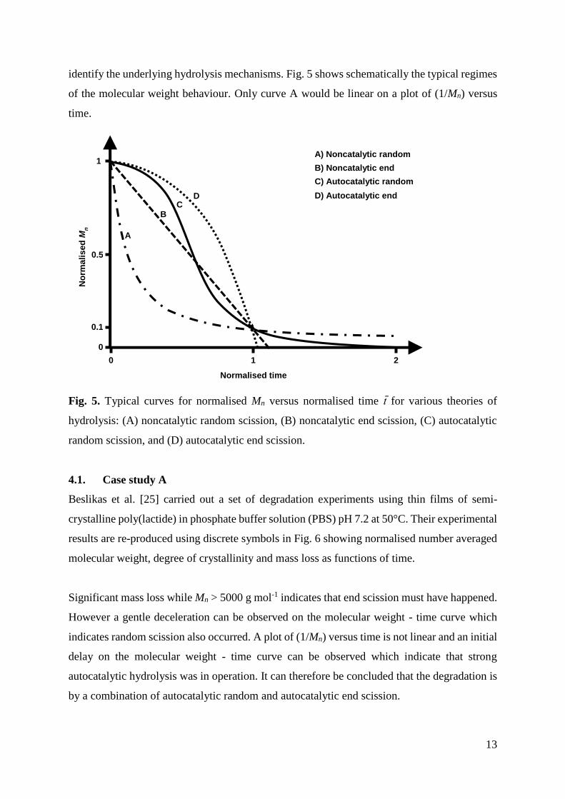
identify the underlying hydrolysis mechanisms. Fig. 5 shows schematically the typical regimes

of the molecular weight behaviour. Only curve A would be linear on a plot of (1/Mn) versus

time.

Fig. 5. Typical curves for normalised Mn versus normalised time t̄ for various theories of

hydrolysis: (A) noncatalytic random scission, (B) noncatalytic end scission, (C) autocatalytic

random scission, and (D) autocatalytic end scission.

4.1. Case study A

Beslikas et al. [25] carried out a set of degradation experiments using thin films of semi-

crystalline poly(lactide) in phosphate buffer solution (PBS) pH 7.2 at 50°C. Their experimental

results are re-produced using discrete symbols in Fig. 6 showing normalised number averaged

molecular weight, degree of crystallinity and mass loss as functions of time.

Significant mass loss while Mn > 5000 g mol-1 indicates that end scission must have happened.

However a gentle deceleration can be observed on the molecular weight - time curve which

indicates random scission also occurred. A plot of (1/Mn) versus time is not linear and an initial

delay on the molecular weight - time curve can be observed which indicate that strong

autocatalytic hydrolysis was in operation. It can therefore be concluded that the degradation is

by a combination of autocatalytic random and autocatalytic end scission.

Normalised time

1

0.5

1 2

0.1

A

B C

D

0

0

A) Noncatalytic random

B) Noncatalytic end

C) Autocatalytic random

D) Autocatalytic end

No

rma

lis

ed

Mn

14

The best fitting between the mathematical model and the data is shown in Fig. 6 using solid

lines. The fitting parameters are provided in Table 1. It is not possible to achieve an equally

good fitting with a different set of hydrolysis mechanisms. Both crystallisation and diffusion

of small chains are included in the numerical model. Crystallite size Vc is estimated from the

literature [45]. It can be observed that the mathematical model can fit the data very well for the

average molecular weight and degree of crystallinity and quite well for mass loss. The best fit

is achieved by kr1 = ke1 = 0, which indicates that the hydrolysis is fully autocatalytic, and

supports the qualitative analysis. The reaction rate ratio of ke2/ kr2 = 7500 indicates that end

scission occurs much faster than random scission. The high rate of end scission is necessary to

produce the level of mass loss observed in the experiment. However it is very important to

point out that the relatively small but finite random scission rate has a major effect on the

molecular weight reduction. The dashed line in Fig. 6 shows the model prediction using

identical set of parameters except that kr2 was set as zero. It can be observed that the small

amount of random scission has a large effect on both molecular weight reduction and mass

loss. A fitting to mass loss may be achieved without random scission by increasing ke2, but a

fitting of molecular weight is not possible. Similarly, a fitting to mass loss is only possible if

end scission is included. Both random and end scission are required to fit the data.

Fig. 6. A model fitting of molecular weight, crystallinity, and mass loss for combined

autocatalytic random scission and autocatalytic end scission as suggested by the qualitative

analysis (solid black lines). For comparison, a fitting without random scission also included

(dashed grey lines). Discrete symbols indicate experimental data [25].

0

2

4

6

8

10

12

14

16

18

20

0

0.1

0.2

0.3

0.4

0.5

0.6

0.7

0.8

0.9

1

0 10 20 30 40 50 60 70

Ma

ss

lo

ss (

%)

No

rma

lis

ed

Mn

/ c

rys

tall

init

y

Time (days)

Best fitting

No random scission

Molecular weight

Crystallinity

Mass loss

15

4.2 Case study B

Batycky et al. [26] carried out degradation experiments of drug-encapsulating microspheres

made of poly(DL-lactide-co-glycolide) 50:50. The samples are amorphous throughout. Their

data are reproduced in Fig. 7 showing normalised number averaged molecular weight and mass

loss as functions of time. From the figure it can be observed that there is clear deceleration on

the molecular weight - time curve indicating random scission. There is an initial delay in the

molecular weight reduction and therefore a plot of (1/Mn) versus time is not linear which

indicates autocatalytic random scission. However, the delay is less significant compared to case

A, perhaps suggesting a noncatalytic hydrolysis contribution. The mass loss is significant while

Mn > 5000 g mol-1 indicating a large end scission rate. The degradation is therefore through a

combination of autocatalytic random and noncatalytic end scission. Batycky et al. [26] also

used a mathematical model to determine whether end or random scission was dominant and

concluded that a combination of both mechanisms was required to fit their data.

The solid lines in Fig. 7 show the best fitting of the model. All the parameters used in the fitting

are provided in Table 1. Again it can be observed that the model is able to fit the experimental

data very well. The best fit was obtained by setting kr1 = ke2 = 0 which indicates noncatalytic

hydrolysis and ke1 / kr2 = 1.26 x105 which indicates end scission occurs much faster than random

scission. Similar to Case A, the large end scission rate is necessary for the observed mass loss

and a similar fitting cannot be achieved by using a different combination of hydrolysis

mechanisms. However the small but finite rate of random scission is critical to the molecular

weight reduction. The dashed lines in Fig. 7 show the model prediction using an identical set

of parameters except that kr1 was set to zero. As with Case A, it can be observed that the small

amount of random scission effects both molecular weight reduction and mass loss. Random

scission is again required to achieve a fitting to the experimental data for molecular weight and

end scission is required for mass loss. The values of diffusion coefficients D0 and Dpore are

chosen to give the best model fitting. They give an indication of the polymer diffusion

coefficients. Significant variation is to be expected between different setups since many factors

affect diffusion. For example, the experiments of Yoon et al. [46] found diffusion coefficients

to be 3 orders of magnitude greater for water molecules in poly(lactide) than poly(glycolide).

16

Fig. 7. A model fitting using a combination of autocatalytic random scission and noncatalytic

end scission (solid black lines) as suggested by the qualitative analysis. A fitting without

random scission is included for reference (dashed grey lines). Experimental data [26] for

molecular weight and mass loss are discrete symbols.

Table 1. Values of the model parameters used in the fittings

Model parameters units Case study A Case study B

M0 g mol-1 72 65 (a)

kr1 day-1 0 0

kr2 [mol-1m3]0.5day-1 3.0 x10-6 8.5 x10-6

ke1 day-1 0 1.26 x105*kr1

ke2 [mol-1m3]0.5day-1 7500*kr2 0

Nchains0 mol m-3 10.4 55

D0 m2 day-1 2.5 x10-11 1.6 x10-15

Dpore m2 day-1 2.5 x10-7 1.6 x10-11

Initial porosity no units 0 0

Ce0 mol-1m3 17,300 17,300

ω mol-1m3 17,300 17,300

Xmax no units 0.655 0

px no units 0.004 0

Vc m3 4.19 x10-24 0

Initial Mn g mol-1 120000 20500

Initial Xc no units 0.5645 0

Film thickness or microsphere radius μm 50 (b) 10

(a) Molar mass is taken as the average of poly(lactide) and poly(glycolide)

(b) Film thickness is not given in the publication so estimated at 50μm.

0

10

20

30

40

50

60

70

80

90

100

0

0.2

0.4

0.6

0.8

1

0 5 10 15 20 25 30

Ma

ss

lo

ss (

%)

No

rma

lis

ed

mo

lecu

lar

we

igh

t

Time (days)

Best fitting

No random scission

Molecular weight

Mass loss

17

5. Review of hydrolysis mechanisms for experimental data available in the literature

The qualitative analysis was applied to experimental data in 31 publications that we could

obtain from the literature [1-31]. Detailed fitting with the mathematical model was also

performed for typical cases. Table 2 lists the identified hydrolysis mechanisms for each

individual paper. Experimental details such as polymer type, initial molecular weight and

minimum dimension of the samples are also provided. The following conclusions can be drawn

from the analysis:

A combination of random and end scission is identified for almost all the data.

Significant molecular weight reduction is always due to random scission.

Mass loss is due to end scission except for thick samples (1.4-2.6mm) for which random

scission may contribute.

Autocatalytic random scission is required for molecular weight reduction in almost all

publications.

Table 2 identifies the hydrolysis mechanisms that are required in order for a fitting to be

achieved. Naturally, the best fitting will be achieved by allowing the model the flexibility to

include all hydrolysis mechanisms to a greater or lesser extent. An important finding is that a

good fitting cannot be achieved without autocatalytic random scission in most cases. Since the

analysis found a mixture of autocatalytic and noncatalytic hydrolysis, it is likely that both types

of hydrolysis mechanism occur depending of the setup of a particular experiment. There have

been several experimental publications that suggest autocatalytic hydrolysis plays a significant

role in degradation under specific conditions. In particular, heterogeneous degradation of large

samples has been attributed to autocatalysis [14, 15, 22, 27, 47, 48], as has the accelerated

degradation of samples with high residual monomer [18, 23], along with the accelerated

degradation of polymers with carboxylic acid end groups versus benzyl alcohol end groups

[27]. However, the findings of the analysis in Table 2 suggest that autocatalytic hydrolysis has

a more important role than noncatalytic hydrolysis over a very broad range of conditions. The

experiments considered in the analysis vary greatly in factors such as sample size and shape,

initial molecular weight, polymer or copolymer type, buffer solution type and temperature,

crystallinity, and the rate of degradation. But the model almost always suggests that

autocatalytic hydrolysis occurs. It is important to note that since end scission is expected, the

monomers that result from end scission control the rate of autocatalytic random scission, and

therefore the rate of Mn reduction. This is due to the fact that the number of monomers is

significantly greater than oligomers, as discussed in Section 3. Since end scission has little or

18

no effect on molecular weight, models that derive the acid catalyst concentration from the value

of molecular weight do not consider the expected situation that end scission controls the

concentration of acid catalyst. Also, an alternative interpretation of the findings of Antheunis

et al. [27] that carboxylic acid end groups accelerate degradation versus benzyl alcohol end

groups could be that the benzyl alcohol end groups are more resistant to end scission so the

initial production of monomers, and therefore catalyst, is retarded.

In the most practical polymers, the initial molecular weight is too large for random scission to

produce enough oligomers by chance in order to give the observed mass loss. However random

scission is crucial in order to give the observed molecular weight reduction. Considering the

experimental data for mass loss presented in Figs. 6 and 7 [25, 26], for the molecular weight to

reduce by 67% only two random scissions per chain are required. It is impossible for this

number of random scissions to produce 3% and 15% mass of oligomers by chance to give the

observed mass loss given that the initial chains contain 1667 and 315 polymer units

respectively. If there is no end scission, the observed mass loss would require that the polymer

chains become water soluble at Mn≈14000 and Mn≈2600 g mol-1 respectively. These values are

much larger than those typically found in the literature which may be in the region of <1000 g

mol-1 [27, 49, 50]. Random scission is only predicted to contribute significantly to mass loss in

publications that used thick samples. This may suggest that random scission is more susceptible

to autocatalysis than end scission because there is likely to be a higher concentration of

oligomers and monomers in the centre of large samples than at the surface or than in smaller

samples where they can more easily diffuse out of the polymer.

It can be generally concluded that ester bonds towards the end of polymer chains are more

susceptible to hydrolysis than those in the middle. If end scission is due to the acidic chain end

folding back on itself, it may be the case that a number of bonds near the chain end can be

cleaved. Experimental measurements of lactic acid monomers would not identify oligomers

produced by this type of end scission so may falsely be interpreted as evidence for random

scission.

19

Table 2. The model is used on a number of degradation experiments to determine the dominant

hydrolysis mechanisms

Ref Polymer type

Initial Mn

(kg mol-1)

Minimum

size (mm)

Scission type

Random scission End scission

Auto-

catalytic

Non-

catalytic

Auto-

catalytic

Non-

catalytic

[1] PLA 70L:30L,D 290 1 YES ONE OF THESE TWO

[2] PLA - L, D, or L/D 500 0.1 YES MAYBE MAYBE MAYBE

[3] PLGA 50DL:50G 10.5 N/A YES YES

[4] PLGA 33 0.05 YES YES

[5] PLLA 550 0.05 YES ONE OF THESE TWO

[6] PLLA 155 0.8 YES YES

[7] PLLA 166 0.8 YES ONE OF THESE TWO

[8] PLLA 100,150 1.5-3 YES ONE OF THESE TWO

PDLLA 27-177 1.5-3 YES MAYBE MAYBE MAYBE

[9] PLA - L, D, or L/D 90 0.05 YES YES

[10] PLA - L, D, or L/D 450 0.05 YES YES

[11] PLLA 45 0.033 YES YES

[12] PLA 50L:50D 450 0.05 YES ONE OF THESE TWO

[13] PLGA - 50DL:50G 14 0.2 YES YES

[14] PDLLA 85 1.5 YES YES

[15] PLLA 72 2 YES YES

[16] PLGA 53 0.2 YES ONE OF THESE TWO

[17] PLLA 550 0.05 YES YES

[18] PLGA 85:15 IV = 1.4dl/g 1.6-3.4 YES ONE OF THESE TWO

[19] PLA 96L:4D 37 2.6 YES ONE OF THESE TWO

[20] PLA 70L:30DL ≈20 2 YES ONE OF THESE TWO

[21] 90PLA:10PCL 28 0.4 YES YES

[22] PDLLA 20-34 2 YES ONE OF THESE TWO

[23] PDLLA 10 0.5 YES YES

[24] PLGA 50:50 28 0.0005-0.022 YES ONE OF THESE TWO

[25] PLLA 120 thin film YES YES

[26] PLGA 50:50 20 microsphere YES YES

[27, 28] PLA, PLGA, PCL 10 1.4-2.3 YES

[29] PLGA 40 0.05 YES

[30] PDLA 100 0.1 YES ONE OF THESE TWO

[31] PLLA 160 2 MAYBE YES MAYBE MAYBE

6. Conclusions

The revised mathematical model was developed to consider degradation by the individual

hydrolysis mechanisms noncatalytic random scission, autocatalytic random scission,

noncatalytic end scission and autocatalytic end scission. The model was able to fit all

experimental degradation data at hand. Simple qualitative trends in the degradation of

molecular weight and mass loss were found to relate to the underlying hydrolysis mechanisms.

These trends are that: 1) a deceleration of molecular weight reduction versus time indicates

random scission whereas a lack of the deceleration indicates end scission; 2) noncatalytic

hydrolysis is indicated by a linear relationship between (1/Mn) and time whereas a nonlinear

relationship indicates autocatalytic hydrolysis; 3) mass loss while the polymer is still medium

to high molecular weight indicates end scission; and 4) a linear increase in mass loss with time

indicates noncatalytic end scission.

20

The experimental degradation data from 31 publications was analysed to identify the most

likely hydrolysis mechanisms using either the qualitative analysis mentioned above or detailed

model fittings. The analysis found that: 1) a combination of random and end scission is almost

always predicted to occur; 2) molecular weight reduction is always due to random scission; 3)

mass loss is due to end scission except for thick samples for which random scission may

contribute; and 4) autocatalytic hydrolysis is expected more often than noncatalytic hydrolysis.

The effects of initial molecular weight and residual monomer are important but are not

investigated in this paper to maintain simplicity. They are analysed in detail in part 2 [39] of

this series of publications.

7. Acknowledgements

Andrew Gleadall acknowledges an EPSRC PhD studentship.

8. References

[1] Lyu, Schley J, Loy B, Lind D, Hobot C, Sparer R, et al. Kinetics and Time-Temperature

Equivalence of Polymer Degradation. Biomacromolecules 2007;8:2301-10.

[2] Tsuji H. Autocatalytic hydrolysis of amorphous-made polylactides: effects of L-lactide

content, tacticity, and enantiomeric polymer blending. Polymer 2002;43:1789-96.

[3] Schliecker G, Schmidt C, Fuchs S, Kissel T. Characterization and in vitro degradation of

poly(2,3-(1,4-diethyl tartrate)-co-2,3-isopropyliden tartrate). Journal of Controlled Release

2004;98:11-23.

[4] Tan HY, Widjaja E, Boey F, Loo SCJ. Spectroscopy techniques for analyzing the hydrolysis

of PLGA and PLLA. Journal of Biomedical Materials Research Part B: Applied Biomaterials

2009;91B:433-40.

[5] Tsuji H, Mizuno A, Ikada Y. Properties and morphology of poly(L-lactide). III. Effects of

initial crystallinity on long-term in vitro hydrolysis of high molecular weight poly(L-lactide)

film in phosphate-buffered solution. Journal of Applied Polymer Science 2000;77:1452-64.

[6] Weir N, Buchanan F, Orr J, Dickson G. Degradation of poly-L-lactide. Part 1: in vitro and

in vivo physiological temperature degradation. Proceedings of the Institution of Mechanical

Engineers, Part H: Journal of Engineering in Medicine 2004;218:307-19.

[7] Weir N, Buchanan F, Orr J, Farrar D, Dickson G. Degradation of poly-L-lactide. Part 2:

increased temperature accelerated degradation. Proceedings of the Institution of Mechanical

Engineers, Part H: Journal of Engineering in Medicine 2004;218:321-30.

21

[8] Migliaresi C, Fambri L, Cohn D. A study on the in vitro degradation of poly(lactic acid).

Journal of Biomaterials Science, Polymer Edition 1994;5:591-606.

[9] Tsuji H. In vitro hydrolysis of blends from enantiomeric poly(lactide)s. Part 1. Well-stereo-

complexed blend and non-blended films. Polymer 2000;41:3621-30.

[10] Tsuji H. In vitro hydrolysis of blends from enantiomeric poly(lactide)s. Part 4: well-homo-

crystallized blend and nonblended films. Biomaterials 2003;24:537-47.

[11] Lam KH, Nieuwenhuis P, Molenaar I, Esselbrugge H, Feijen J, Dijkstra PJ, et al.

Biodegradation of porous versus non-porous poly(L-lactic acid) films. Journal of Materials

Science: Materials in Medicine 1994;5:181-9.

[12] Tsuji H, Del Carpio CA. In Vitro Hydrolysis of Blends from Enantiomeric Poly(lactide)s.

3. Homocrystallized and Amorphous Blend Films. Biomacromolecules 2002;4:7-11.

[13] Schliecker G, Schmidt C, Fuchs S, Wombacher R, Kissel T. Hydrolytic degradation of

poly(lactide-co-glycolide) films: effect of oligomers on degradation rate and crystallinity.

International Journal of Pharmaceutics 2003;266:39-49.

[14] Li S, McCarthy S. Further investigations on the hydrolytic degradation of poly (DL-

lactide). Biomaterials 1999;20:35-44.

[15] Li SM, Garreau H, Vert M. Structure-property relationships in the case of the degradation

of massive poly(α-hydroxy acids) in aqueous media. Journal of Materials Science: Materials

in Medicine 1990;1:198-206.

[16] Cai Q, Shi G, Bei J, Wang S. Enzymatic degradation behavior and mechanism of

Poly(lactide-co-glycolide) foams by trypsin. Biomaterials 2003;24:629-38.

[17] Tsuji H, Ikada Y. Properties and morphology of poly(L-lactide) 4. Effects of structural

parameters on long-term hydrolysis of poly(L-lactide) in phosphate-buffered solution. Polymer

Degradation and Stability 2000;67:179-89.

[18] Paakinaho K, Heino H, Väisänen J, Törmälä P, Kellomäki M. Effects of lactide monomer

on the hydrolytic degradation of poly(lactide-co-glycolide) 85L/15G. Journal of the

Mechanical Behavior of Biomedical Materials 2011;4:1283-90.

[19] Niemelä T. Effect of β-tricalcium phosphate addition on the in vitro degradation of self-

reinforced poly-l,d-lactide. Polymer Degradation and Stability 2005;89:492-500.

[20] Niiranen H, Pyhältö T, Rokkanen P, Kellomäki M, Törmälä P. In vitro and in vivo

behavior of self-reinforced bioabsorbable polymer and self-reinforced bioabsorbable

polymer/bioactive glass composites. Journal of Biomedical Materials Research Part A

2004;69A:699-708.

22

[21] Vieira AC, Vieira JC, Ferra JM, Magalhães FD, Guedes RM, Marques AT. Mechanical

study of PLA–PCL fibers during in vitro degradation. Journal of the Mechanical Behavior of

Biomedical Materials 2011;4:451-60.

[22] Grizzi I, Garreau H, Li S, Vert M. Hydrolytic degradation of devices based on poly(dl-

lactic acid) size-dependence. Biomaterials 1995;16:305-11.

[23] Hyon SH, Jamshidi K, Ikada Y. Effects of residual monomer on the degradation of DL-

lactide polymer. Polymer International 1998;46:196-202.

[24] Dunne M, Corrigan OI, Ramtoola Z. Influence of particle size and dissolution conditions

on the degradation properties of polylactide-co-glycolide particles. Biomaterials

2000;21:1659-68.

[25] Beslikas T, Gigis I, Goulios V, Christoforides J, Papageorgiou GZ, Bikiaris DN.

Crystallization Study and Comparative in Vitro-in Vivo Hydrolysis of PLA Reinforcement

Ligament. International journal of molecular sciences 2011;12:6597-618.

[26] Batycky RP, Hanes J, Langer R, Edwards DA. A theoretical model of erosion and

macromolecular drug release from biodegrading microspheres. Journal of Pharmaceutical

Sciences 1997;86:1464-77.

[27] Antheunis H, van der Meer J-C, de Geus M, Kingma W, Koning CE. Improved

Mathematical Model for the Hydrolytic Degradation of Aliphatic Polyesters. Macromolecules

2009;42:2462-71.

[28] Antheunis H, van der Meer J-C, de Geus M, Heise A, Koning CE. Autocatalytic Equation

Describing the Change in Molecular Weight during Hydrolytic Degradation of Aliphatic

Polyesters. Biomacromolecules 2010;11:1118-24.

[29] Raman C, Berkland C, Kim K, Pack DW. Modeling small-molecule release from PLG

microspheres: effects of polymer degradation and nonuniform drug distribution. Journal of

Controlled Release 2005;103:149-58.

[30] Pitt GG, Gratzl MM, Kimmel GL, Surles J, Sohindler A. Aliphatic polyesters II. The

degradation of poly (DL-lactide), poly (ε-caprolactone), and their copolymers in vivo.

Biomaterials 1981;2:215-20.

[31] Pistner H, Bendi DR, Mühling J, Reuther JF. Poly (l-lactide): a long-term degradation

study in vivo: Part III. Analytical characterization. Biomaterials 1993;14:291-8.

[32] Wang Y, Pan J, Han X, Sinka C, Ding L. A phenomenological model for the degradation

of biodegradable polymers. Biomaterials 2008;29:3393-401.

[33] Han X, Pan J. A model for simultaneous crystallisation and biodegradation of

biodegradable polymers. Biomaterials 2009;30:423-30.

23

[34] Han X, Pan J, Buchanan F, Weir N, Farrar D. Analysis of degradation data of poly(l-

lactide-co-l,d-lactide) and poly(l-lactide) obtained at elevated and physiological temperatures

using mathematical models. Acta Biomaterialia 2010;6:3882-9.

[35] Gleadall A, Pan J, Atkinson H. A simplified theory of crystallisation induced by polymer

chain scissions for biodegradable polyesters. Polymer Degradation and Stability 2012;97:1616-

20.

[36] Shih C. Chain-end scission in acid catalyzed hydrolysis of poly (D,L-lactide) in solution.

Journal of Controlled Release 1995;34:9-15.

[37] Siparsky GL, Voorhees KJ, Miao F. Hydrolysis of polylactic acid (PLA) and

polycaprolactone (PCL) in aqueous acetonitrile solutions: Autocatalysis. Journal of

Environmental Polymer Degradation 1998;6:31-41.

[38] Buchanan FJ. Degradation rate of bioresorbable materials: Prediction and evaluation.

Cambridge, England/Boca Raton [FL]: Woodhead Publishing/CRC Press; 2008.

[39] Gleadall A, Pan J, Kruft M-A. Degradation mechanisms of bioresorbable polyesters, part

2: effects of initial molecular weight and residual monomer. Acta Biomaterialia.

[40] Wiggins JS, Hassan MK, Mauritz KA, Storey RF. Hydrolytic degradation of poly(d,l-

lactide) as a function of end group: Carboxylic acid vs. hydroxyl. Polymer 2006;47:1960-9.

[41] Flory PJ. Principles of Polymer Chemistry. Ithaca, NY: Cornell University Press; 1955.

[42] Avrami M. Kinetics of phase change. I General theory. The Journal of Chemical Physics

1939;7:1103-12.

[43] Avrami M. Kinetics of phase change. II Transformation-time relations for random

distribution of nuclei. The Journal of Chemical Physics 1940;8:212-24.

[44] Avrami M. Granulation, phase change, and microstructure kinetics of phase change. III.

The Journal of Chemical Physics 1941;9:177-84.

[45] Zong X-H, Wang Z-G, Hsiao BS, Chu B, Zhou JJ, Jamiolkowski DD, et al. Structure and

morphology changes in absorbable poly(glycolide) and poly(glycolide-co-lactide) during in

vitro degradation. Macromolecules 1999;32:8107-14.

[46] Yoon J-S, Jung H-W, Kim M-N, Park E-S. Diffusion coefficient and equilibrium solubility

of water molecules in biodegradable polymers. Journal of Applied Polymer Science

2000;77:1716-22.

[47] Li SM, Garreau H, Vert M. Structure-property relationships in the case of the degradation

of massive aliphatic poly-(α-hydroxy acids) in aqueous media. Journal of Materials Science:

Materials in Medicine 1990;1:123-30.

24

[48] Li SM, Garreau H, Vert M. Structure-property relationships in the case of the degradation

of massive poly(α-hydroxy acids) in aqueous media. Journal of Materials Science: Materials

in Medicine 1990;1:131-9.

[49] Vey E, Roger C, Meehan L, Booth J, Claybourn M, Miller AF, et al. Degradation

mechanism of poly(lactic-co-glycolic) acid block copolymer cast films in phosphate buffer

solution. Polymer Degradation and Stability 2008;93:1869-76.

[50] Schliecker G, Schmidt C, Fuchs S, Kissel T. Characterization of a homologous series of

d,l-lactic acid oligomers; a mechanistic study on the degradation kinetics in vitro. Biomaterials

2003;24:3835-44.