degree centrality closeness centrality betweenness ...€¦ · conks @networksvox measures of...
TRANSCRIPT
CoNKs@networksvoxMeasures ofcentrality
Background
CentralitymeasuresDegree centralityCloseness centralityBetweennessEigenvalue centralityHubs and Authorities
References
What’sC
theStory?s
KNo
Really,
..........
.....
.1 of 28
Measures of centralityComplex Networks | @networksvox
CSYS/MATH 303, Spring, 2014 | #SpringCoNKs2014
Prof. Peter Dodds | @peterdodds
Dept. of Mathematics & Statistics | Vermont Complex Systems CenterVermont Advanced Computing Core | University of Vermont
What’sC
theStory?s
KNo
Really,
Licensed under the Creative Commons Attribution-NonCommercial-ShareAlike 3.0 License.

CoNKs@networksvoxMeasures ofcentrality
Background
CentralitymeasuresDegree centralityCloseness centralityBetweennessEigenvalue centralityHubs and Authorities
References
What’sC
theStory?s
KNo
Really,
..........
.....
.2 of 28
These slides are brought to you by:
CoNKs@networksvoxMeasures ofcentrality
Background
CentralitymeasuresDegree centralityCloseness centralityBetweennessEigenvalue centralityHubs and Authorities
References
What’sC
theStory?s
KNo
Really,
..........
.....
.3 of 28
Outline
Background
Centrality measuresDegree centralityCloseness centralityBetweennessEigenvalue centralityHubs and Authorities
References
CoNKs@networksvoxMeasures ofcentrality
Background
CentralitymeasuresDegree centralityCloseness centralityBetweennessEigenvalue centralityHubs and Authorities
References
What’sC
theStory?s
KNo
Really,
..........
.....
.4 of 28
How big is my node?
▶ Basic question: how ‘important’ are specific nodes andedges in a network?
▶ An important node or edge might:1. handle a relatively large amount of the network’s traffic
(e.g., cars, information);2. bridge two or more distinct groups (e.g., liason,
interpreter);3. be a source of important ideas, knowledge, or
judgments (e.g., supreme court decisions, an employeewho ‘knows where everything is’).
▶ So how do we quantify such a slippery concept asimportance?
▶ We generate ad hoc, reasonable measures, and examinetheir utility...
CoNKs@networksvoxMeasures ofcentrality
Background
CentralitymeasuresDegree centralityCloseness centralityBetweennessEigenvalue centralityHubs and Authorities
References
What’sC
theStory?s
KNo
Really,
..........
.....
.5 of 28
Centrality
▶ One possible reflection of importance is centrality.▶ Presumption is that nodes or edges that are (in some
sense) in the middle of a network are important for thenetwork’s function.
▶ Idea of centrality comes from social networksliterature [7].
▶ Many flavors of centrality...1. Many are topological and quasi-dynamical;2. Some are based on dynamics (e.g., traffic).
▶ We will define and examine a few...▶ (Later: see centrality useful in identifying communities
in networks.)
CoNKs@networksvoxMeasures ofcentrality
Background
CentralitymeasuresDegree centralityCloseness centralityBetweennessEigenvalue centralityHubs and Authorities
References
What’sC
theStory?s
KNo
Really,
..........
.....
.7 of 28
Centrality
.Degree centrality..
.
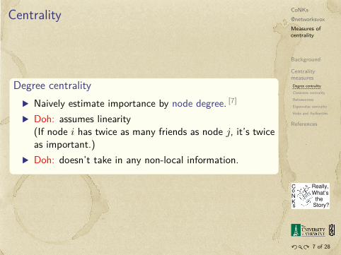
▶ Naively estimate importance by node degree. [7]
▶ Doh: assumes linearity(If node 𝑖 has twice as many friends as node 𝑗, it’s twiceas important.)
▶ Doh: doesn’t take in any non-local information.
CoNKs@networksvoxMeasures ofcentrality
Background
CentralitymeasuresDegree centralityCloseness centralityBetweennessEigenvalue centralityHubs and Authorities
References
What’sC
theStory?s
KNo
Really,
..........
.....
.9 of 28
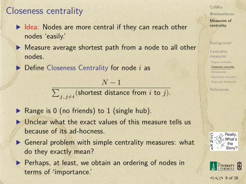
Closeness centrality▶ Idea: Nodes are more central if they can reach other
nodes ‘easily.’▶ Measure average shortest path from a node to all other
nodes.▶ Define Closeness Centrality for node 𝑖 as
𝑁 − 1∑𝑗,𝑗≠𝑖(shortest distance from 𝑖 to 𝑗).
▶ Range is 0 (no friends) to 1 (single hub).▶ Unclear what the exact values of this measure tells us
because of its ad-hocness.▶ General problem with simple centrality measures: what
do they exactly mean?▶ Perhaps, at least, we obtain an ordering of nodes in
terms of ‘importance.’
CoNKs@networksvoxMeasures ofcentrality
Background
CentralitymeasuresDegree centralityCloseness centralityBetweennessEigenvalue centralityHubs and Authorities
References
What’sC
theStory?s
KNo
Really,
..........
.....
.11 of 28
Betweenness centrality
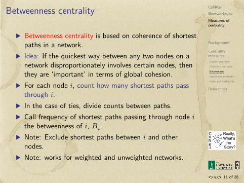
▶ Betweenness centrality is based on coherence of shortestpaths in a network.
▶ Idea: If the quickest way between any two nodes on anetwork disproportionately involves certain nodes, thenthey are ‘important’ in terms of global cohesion.
▶ For each node 𝑖, count how many shortest paths passthrough 𝑖.
▶ In the case of ties, divide counts between paths.▶ Call frequency of shortest paths passing through node 𝑖
the betweenness of 𝑖, 𝐵𝑖.▶ Note: Exclude shortest paths between 𝑖 and other
nodes.▶ Note: works for weighted and unweighted networks.
CoNKs@networksvoxMeasures ofcentrality
Background
CentralitymeasuresDegree centralityCloseness centralityBetweennessEigenvalue centralityHubs and Authorities
References
What’sC
theStory?s
KNo
Really,
..........
.....
.12 of 28
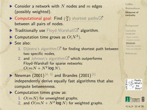
▶ Consider a network with 𝑁 nodes and 𝑚 edges(possibly weighted).
▶ Computational goal: Find (𝑁2 ) shortest pathsbetween all pairs of nodes.
▶ Traditionally use Floyd-Warshall algorithm.▶ Computation time grows as 𝑂(𝑁3).▶ See also:
1. Dijkstra’s algorithm for finding shortest path betweentwo specific nodes,
2. and Johnson’s algorithm which outperformsFloyd-Warshall for sparse networks:𝑂(𝑚𝑁 + 𝑁2 log𝑁).
▶ Newman (2001) [4, 5] and Brandes (2001) [1]
independently derive equally fast algorithms that alsocompute betweenness.
▶ Computation times grow as:1. 𝑂(𝑚𝑁) for unweighted graphs;2. and 𝑂(𝑚𝑁 + 𝑁2 log𝑁) for weighted graphs.
CoNKs@networksvoxMeasures ofcentrality
Background
CentralitymeasuresDegree centralityCloseness centralityBetweennessEigenvalue centralityHubs and Authorities
References
What’sC
theStory?s
KNo
Really,
..........
.....
.13 of 28
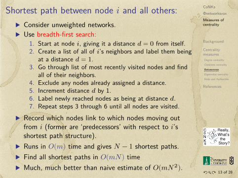
Shortest path between node 𝑖 and all others:▶ Consider unweighted networks.▶ Use breadth-first search:
1. Start at node 𝑖, giving it a distance 𝑑 = 0 from itself.2. Create a list of all of 𝑖’s neighbors and label them being
at a distance 𝑑 = 1.3. Go through list of most recently visited nodes and find
all of their neighbors.4. Exclude any nodes already assigned a distance.5. Increment distance 𝑑 by 1.6. Label newly reached nodes as being at distance 𝑑.7. Repeat steps 3 through 6 until all nodes are visited.
▶ Record which nodes link to which nodes moving outfrom 𝑖 (former are ‘predecessors’ with respect to 𝑖’sshortest path structure).
▶ Runs in 𝑂(𝑚) time and gives 𝑁 − 1 shortest paths.▶ Find all shortest paths in 𝑂(𝑚𝑁) time▶ Much, much better than naive estimate of 𝑂(𝑚𝑁2).

CoNKs@networksvoxMeasures ofcentrality
Background
CentralitymeasuresDegree centralityCloseness centralityBetweennessEigenvalue centralityHubs and Authorities
References
What’sC
theStory?s
KNo
Really,
..........
.....
.14 of 28
Newman’s Betweenness algorithm: [4]
pears not to influence the results highly. The recalculation
step, on the other hand, is absolutely crucial to the operation
of our methods. This step was missing from previous at-
tempts at solving the clustering problem using divisive algo-
rithms, and yet without it the results are very poor indeed,
failing to find known community structure even in the sim-
plest of cases. In Sec. VB we give an example comparing
the performance of the algorithm on a particular network
with and without the recalculation step.
In the following sections, we discuss implementation and
give examples of our algorithms for finding community
structure. For the reader who merely wants to know what
algorithm they should use for their own problem, let us give
an immediate answer: for most problems, we recommend the
algorithm with betweenness scores calculated using the
shortest-path betweenness measure !i" above. This measureappears to work well and is the quickest to calculate—as
described in Sec. III A, it can be calculated for all edges in
time O(mn), where m is the number of edges in the graph
and n is the number of vertices #48$. This is the only versionof the algorithm that we discussed in Ref. #25$. The otherversions we discuss, while being of some pedagogical inter-
est, make greater computational demands, and in practice
seem to give results no better than the shortest-path method.
III. IMPLEMENTATION
In theory, the descriptions of the preceding section com-
pletely define the methods we consider in this paper, but in
practice there are a number of subtleties to their implemen-
tation that are important for turning the description into a
workable computer algorithm.
Essentially all of the work in the algorithm is in the cal-
culation of the betweenness scores for the edges; the job of
finding and removing the highest-scoring edge is trivial and
not computationally demanding. Let us tackle our three sug-
gested betweenness measures in turn.
A. Shortest-path betweenness
At first sight, it appears that calculating the edge between-
ness measure based on geodesic paths for all edges will take
O(mn2) operations on a graph with m edges and n vertices:
calculating the shortest path between a particular pair of ver-
tices can be done using breadth-first search in time O(m)
#28,29$, and there are O(n2) vertex pairs. Recently, however,new algorithms have been proposed by Newman #30$ andindependently by Brandes #31$ that can perform the calcula-
tion faster than this, finding all betweennesses in O(mn)
time. Both Newman and Brandes gave algorithms for the
standard Freeman vertex betweenness, but it is trivial to
adapt their algorithms for edge betweenness. We describe the
resulting method here for the algorithm of Newman.
Breadth-first search can find shortest paths from a single
vertex s to all others in time O(m). In the simplest case,
when there is only a single shortest path from the source
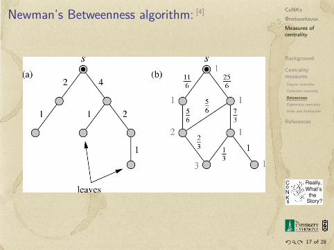
vertex to any other !we will consider other cases in a mo-ment", the resulting set of paths forms a shortest-path tree—see Fig. 4!a". We can use this tree to calculate the contribu-
tion to betweenness for each edge from this set of paths as
follows. We find first the ‘‘leaves’’ of the tree, i.e., those
nodes such that no shortest paths to other nodes pass through
them, and we assign a score of 1 to the single edge that
connects each to the rest of the tree, as shown in the figure.
Then, starting with those edges that are farthest from the
source vertex on the tree, i.e., lowest in Fig. 4!a", we workupwards, assigning a score to each edge that is 1 plus the
sum of the scores on the neighboring edges immediately be-
low it !i.e., those edges with which it shares a common ver-tex". When we have gone though all edges in the tree, theresulting scores are the betweenness counts for the paths
from vertex s. Repeating the process for all possible vertices
s and summing the scores, we arrive at the full betweenness
scores for shortest paths between all pairs. The breadth-first
search and the process of working up through the tree both
take worst-case time O(m) and there are n vertices total, so
the entire calculation takes time O(mn) as claimed.
This simple case serves to illustrate the basic principle
behind the algorithm. In general, however, it is not the case
that there is only a single shortest path between any pair of
vertices. Most networks have at least some vertex pairs be-
tween which there are two or more geodesic paths of equal
length. Figure 4!b" shows a simple example of a shortestpath ‘‘tree’’ for a network with this property. The resulting
structure is in fact no longer a tree, and in such cases an extra
step is required in the algorithm to calculate the betweenness
correctly.
In the traditional definition of vertex betweenness #27$,multiple shortest paths between a pair of vertices are given
equal weights summing to 1. For example, if there are three
shortest paths, each will be given weight 13. We adopt the
same definition for our edge betweenness !as did Anthonissein his original work #26$, although other definitions are pos-
FIG. 4. Calculation of shortest-path betweenness: !a" Whenthere is only a single shortest path from a source vertex s !top" to allother reachable vertices, those paths necessarily form a tree, which
makes the calculation of the contribution to betweenness from this
set of paths particularly simple, as described in the text. !b" Forcases in which there is more than one shortest path to some vertices,
the calculation is more complex. First we must calculate the number
of distinct paths from the source s to each vertex !numbers onvertices", and then these are used to weight the path counts asdescribed in the text. In either case, we can check the results by
confirming that the sum of the betweennesses of the edges con-
nected to the source vertex is equal to the total number of reachable
vertices—six in each of the cases illustrated here.
M. E. J. NEWMAN AND M. GIRVAN PHYSICAL REVIEW E 69, 026113 !2004"
026113-4
CoNKs@networksvoxMeasures ofcentrality
Background
CentralitymeasuresDegree centralityCloseness centralityBetweennessEigenvalue centralityHubs and Authorities
References
What’sC
theStory?s
KNo
Really,
..........
.....
.15 of 28
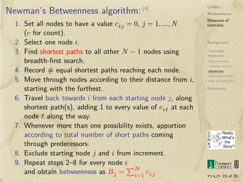
Newman’s Betweenness algorithm: [4]
1. Set all nodes to have a value 𝑐𝑖𝑗 = 0, 𝑗 = 1, ..., 𝑁(𝑐 for count).
2. Select one node 𝑖.3. Find shortest paths to all other 𝑁 − 1 nodes using
breadth-first search.4. Record # equal shortest paths reaching each node.5. Move through nodes according to their distance from 𝑖,
starting with the furthest.6. Travel back towards 𝑖 from each starting node 𝑗, along
shortest path(s), adding 1 to every value of 𝑐𝑖ℓ at eachnode ℓ along the way.
7. Whenever more than one possibility exists, apportionaccording to total number of short paths comingthrough predecessors.
8. Exclude starting node 𝑗 and 𝑖 from increment.9. Repeat steps 2–8 for every node 𝑖
and obtain betweenness as 𝐵𝑗 = ∑𝑁𝑖=1 𝑐𝑖𝑗.
CoNKs@networksvoxMeasures ofcentrality
Background
CentralitymeasuresDegree centralityCloseness centralityBetweennessEigenvalue centralityHubs and Authorities
References
What’sC
theStory?s
KNo
Really,
..........
.....
.16 of 28
Newman’s Betweenness algorithm: [4]
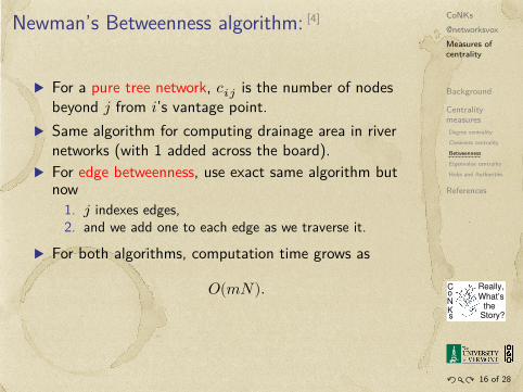
▶ For a pure tree network, 𝑐𝑖𝑗 is the number of nodesbeyond 𝑗 from 𝑖’s vantage point.
▶ Same algorithm for computing drainage area in rivernetworks (with 1 added across the board).
▶ For edge betweenness, use exact same algorithm butnow
1. 𝑗 indexes edges,2. and we add one to each edge as we traverse it.
▶ For both algorithms, computation time grows as
𝑂(𝑚𝑁).
CoNKs@networksvoxMeasures ofcentrality
Background
CentralitymeasuresDegree centralityCloseness centralityBetweennessEigenvalue centralityHubs and Authorities
References
What’sC
theStory?s
KNo
Really,
..........
.....
.17 of 28
Newman’s Betweenness algorithm: [4]
pears not to influence the results highly. The recalculation
step, on the other hand, is absolutely crucial to the operation
of our methods. This step was missing from previous at-
tempts at solving the clustering problem using divisive algo-
rithms, and yet without it the results are very poor indeed,
failing to find known community structure even in the sim-
plest of cases. In Sec. VB we give an example comparing
the performance of the algorithm on a particular network
with and without the recalculation step.
In the following sections, we discuss implementation and
give examples of our algorithms for finding community
structure. For the reader who merely wants to know what
algorithm they should use for their own problem, let us give
an immediate answer: for most problems, we recommend the
algorithm with betweenness scores calculated using the
shortest-path betweenness measure !i" above. This measureappears to work well and is the quickest to calculate—as
described in Sec. III A, it can be calculated for all edges in
time O(mn), where m is the number of edges in the graph
and n is the number of vertices #48$. This is the only versionof the algorithm that we discussed in Ref. #25$. The otherversions we discuss, while being of some pedagogical inter-
est, make greater computational demands, and in practice
seem to give results no better than the shortest-path method.
III. IMPLEMENTATION
In theory, the descriptions of the preceding section com-
pletely define the methods we consider in this paper, but in
practice there are a number of subtleties to their implemen-
tation that are important for turning the description into a
workable computer algorithm.
Essentially all of the work in the algorithm is in the cal-
culation of the betweenness scores for the edges; the job of
finding and removing the highest-scoring edge is trivial and
not computationally demanding. Let us tackle our three sug-
gested betweenness measures in turn.
A. Shortest-path betweenness
At first sight, it appears that calculating the edge between-
ness measure based on geodesic paths for all edges will take
O(mn2) operations on a graph with m edges and n vertices:
calculating the shortest path between a particular pair of ver-
tices can be done using breadth-first search in time O(m)
#28,29$, and there are O(n2) vertex pairs. Recently, however,new algorithms have been proposed by Newman #30$ andindependently by Brandes #31$ that can perform the calcula-
tion faster than this, finding all betweennesses in O(mn)
time. Both Newman and Brandes gave algorithms for the
standard Freeman vertex betweenness, but it is trivial to
adapt their algorithms for edge betweenness. We describe the
resulting method here for the algorithm of Newman.
Breadth-first search can find shortest paths from a single
vertex s to all others in time O(m). In the simplest case,
when there is only a single shortest path from the source
vertex to any other !we will consider other cases in a mo-ment", the resulting set of paths forms a shortest-path tree—see Fig. 4!a". We can use this tree to calculate the contribu-
tion to betweenness for each edge from this set of paths as
follows. We find first the ‘‘leaves’’ of the tree, i.e., those
nodes such that no shortest paths to other nodes pass through
them, and we assign a score of 1 to the single edge that
connects each to the rest of the tree, as shown in the figure.
Then, starting with those edges that are farthest from the
source vertex on the tree, i.e., lowest in Fig. 4!a", we workupwards, assigning a score to each edge that is 1 plus the
sum of the scores on the neighboring edges immediately be-
low it !i.e., those edges with which it shares a common ver-tex". When we have gone though all edges in the tree, theresulting scores are the betweenness counts for the paths
from vertex s. Repeating the process for all possible vertices
s and summing the scores, we arrive at the full betweenness
scores for shortest paths between all pairs. The breadth-first
search and the process of working up through the tree both
take worst-case time O(m) and there are n vertices total, so
the entire calculation takes time O(mn) as claimed.
This simple case serves to illustrate the basic principle
behind the algorithm. In general, however, it is not the case
that there is only a single shortest path between any pair of
vertices. Most networks have at least some vertex pairs be-
tween which there are two or more geodesic paths of equal
length. Figure 4!b" shows a simple example of a shortestpath ‘‘tree’’ for a network with this property. The resulting
structure is in fact no longer a tree, and in such cases an extra
step is required in the algorithm to calculate the betweenness
correctly.
In the traditional definition of vertex betweenness #27$,multiple shortest paths between a pair of vertices are given
equal weights summing to 1. For example, if there are three
shortest paths, each will be given weight 13. We adopt the
same definition for our edge betweenness !as did Anthonissein his original work #26$, although other definitions are pos-
FIG. 4. Calculation of shortest-path betweenness: !a" Whenthere is only a single shortest path from a source vertex s !top" to allother reachable vertices, those paths necessarily form a tree, which
makes the calculation of the contribution to betweenness from this
set of paths particularly simple, as described in the text. !b" Forcases in which there is more than one shortest path to some vertices,
the calculation is more complex. First we must calculate the number
of distinct paths from the source s to each vertex !numbers onvertices", and then these are used to weight the path counts asdescribed in the text. In either case, we can check the results by
confirming that the sum of the betweennesses of the edges con-
nected to the source vertex is equal to the total number of reachable
vertices—six in each of the cases illustrated here.
M. E. J. NEWMAN AND M. GIRVAN PHYSICAL REVIEW E 69, 026113 !2004"
026113-4
CoNKs@networksvoxMeasures ofcentrality
Background
CentralitymeasuresDegree centralityCloseness centralityBetweennessEigenvalue centralityHubs and Authorities
References
What’sC
theStory?s
KNo
Really,
..........
.....
.19 of 28
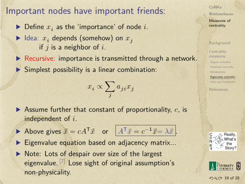
Important nodes have important friends:▶ Define 𝑥𝑖 as the ‘importance’ of node 𝑖.▶ Idea: 𝑥𝑖 depends (somehow) on 𝑥𝑗
if 𝑗 is a neighbor of 𝑖.▶ Recursive: importance is transmitted through a network.▶ Simplest possibility is a linear combination:
𝑥𝑖 ∝ ∑𝑗
𝑎𝑗𝑖𝑥𝑗
▶ Assume further that constant of proportionality, 𝑐, isindependent of 𝑖.
▶ Above gives 𝑥 = 𝑐𝐴T 𝑥 or 𝐴T 𝑥 = 𝑐−1 𝑥= 𝜆 𝑥 .▶ Eigenvalue equation based on adjacency matrix...▶ Note: Lots of despair over size of the largest
eigenvalue. [7] Lose sight of original assumption’snon-physicality.
CoNKs@networksvoxMeasures ofcentrality
Background
CentralitymeasuresDegree centralityCloseness centralityBetweennessEigenvalue centralityHubs and Authorities
References
What’sC
theStory?s
KNo
Really,
..........
.....
.20 of 28
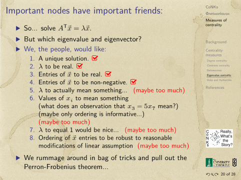
Important nodes have important friends:▶ So... solve 𝐴T 𝑥 = 𝜆 𝑥.▶ But which eigenvalue and eigenvector?▶ We, the people, would like:
1. A unique solution. 2. 𝜆 to be real. 3. Entries of �� to be real. 4. Entries of �� to be non-negative. 5. 𝜆 to actually mean something... (maybe too much)6. Values of 𝑥𝑖 to mean something
(what does an observation that 𝑥3 = 5𝑥7 mean?)(maybe only ordering is informative...)(maybe too much)
7. 𝜆 to equal 1 would be nice... (maybe too much)8. Ordering of �� entries to be robust to reasonable
modifications of linear assumption (maybe too much)▶ We rummage around in bag of tricks and pull out the
Perron-Frobenius theorem...
CoNKs@networksvoxMeasures ofcentrality
Background
CentralitymeasuresDegree centralityCloseness centralityBetweennessEigenvalue centralityHubs and Authorities
References
What’sC
theStory?s
KNo
Really,
..........
.....
.21 of 28
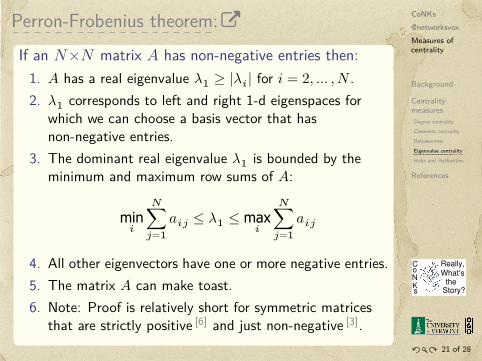
Perron-Frobenius theorem:.If an 𝑁×𝑁 matrix 𝐴 has non-negative entries then:..
.
1. 𝐴 has a real eigenvalue 𝜆1 ≥ |𝜆𝑖| for 𝑖 = 2, … , 𝑁 .2. 𝜆1 corresponds to left and right 1-d eigenspaces for
which we can choose a basis vector that hasnon-negative entries.
3. The dominant real eigenvalue 𝜆1 is bounded by theminimum and maximum row sums of 𝐴:
min𝑖
𝑁∑𝑗=1
𝑎𝑖𝑗 ≤ 𝜆1 ≤ max𝑖
𝑁∑𝑗=1
𝑎𝑖𝑗
4. All other eigenvectors have one or more negative entries.5. The matrix 𝐴 can make toast.6. Note: Proof is relatively short for symmetric matrices
that are strictly positive [6] and just non-negative [3].
CoNKs@networksvoxMeasures ofcentrality
Background
CentralitymeasuresDegree centralityCloseness centralityBetweennessEigenvalue centralityHubs and Authorities
References
What’sC
theStory?s
KNo
Really,
..........
.....
.22 of 28
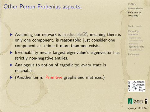
Other Perron-Frobenius aspects:
▶ Assuming our network is irreducible, meaning there isonly one component, is reasonable: just consider onecomponent at a time if more than one exists.
▶ Irreducibility means largest eigenvalue’s eigenvector hasstrictly non-negative entries.
▶ Analogous to notion of ergodicity: every state isreachable.
▶ (Another term: Primitive graphs and matrices.)
CoNKs@networksvoxMeasures ofcentrality
Background
CentralitymeasuresDegree centralityCloseness centralityBetweennessEigenvalue centralityHubs and Authorities
References
What’sC
theStory?s
KNo
Really,
..........
.....
.24 of 28
Hubs and Authorities
▶ Generalize eigenvalue centrality to allow nodes to havetwo attributes:
1. Authority: how much knowledge, information, etc., heldby a node on a topic.
2. Hubness (or Hubosity or Hubbishness or Hubtasticness):how well a node ‘knows’ where to find information on agiven topic.
▶ Original work due to the legendary Jon Kleinberg. [2]
▶ Best hubs point to best authorities.▶ Recursive: Hubs authoritatively link to hubs, authorities
hubbishly link to other authorities.▶ More: look for dense links between sets of ‘good’ hubs
pointing to sets of ‘good’ authorities.▶ Known as the HITS algorithm
(Hyperlink-Induced Topics Search).
CoNKs@networksvoxMeasures ofcentrality
Background
CentralitymeasuresDegree centralityCloseness centralityBetweennessEigenvalue centralityHubs and Authorities
References
What’sC
theStory?s
KNo
Really,
..........
.....
.25 of 28
Hubs and Authorities▶ Give each node two scores:
1. 𝑥𝑖 = authority score for node 𝑖2. 𝑦𝑖 = hubtasticness score for node 𝑖
▶ As for eigenvector centrality, we connect the scores ofneighboring nodes.
▶ New story I: a good authority is linked to by good hubs.▶ Means 𝑥𝑖 should increase as ∑𝑁
𝑗=1 𝑎𝑗𝑖𝑦𝑗 increases.▶ Note: indices are 𝑗𝑖 meaning 𝑗 has a directed link to 𝑖.▶ New story II: good hubs point to good authorities.▶ Means 𝑦𝑖 should increase as ∑𝑁
𝑗=1 𝑎𝑖𝑗𝑥𝑗 increases.▶ Linearity assumption:
𝑥 ∝ 𝐴𝑇 𝑦 and 𝑦 ∝ 𝐴 𝑥
CoNKs@networksvoxMeasures ofcentrality
Background
CentralitymeasuresDegree centralityCloseness centralityBetweennessEigenvalue centralityHubs and Authorities
References
What’sC
theStory?s
KNo
Really,
..........
.....
.26 of 28
Hubs and Authorities
▶ So let’s say we have
𝑥 = 𝑐1𝐴𝑇 𝑦 and 𝑦 = 𝑐2𝐴 𝑥
where 𝑐1 and 𝑐2 must be positive.▶ Above equations combine to give
𝑥 = 𝑐1𝐴𝑇 𝑐2𝐴 𝑥 = 𝜆𝐴𝑇 𝐴 𝑥.
where 𝜆 = 𝑐1𝑐2 > 0.▶ It’s all good: we have the heart of singular value
decomposition before us...
CoNKs@networksvoxMeasures ofcentrality
Background
CentralitymeasuresDegree centralityCloseness centralityBetweennessEigenvalue centralityHubs and Authorities
References
What’sC
theStory?s
KNo
Really,
..........
.....
.27 of 28
We can do this:
▶ 𝐴𝑇 𝐴 is symmetric.▶ 𝐴𝑇 𝐴 is semi-positive definite so its eigenvalues are all
≥ 0.▶ 𝐴𝑇 𝐴’s eigenvalues are the square of 𝐴’s singular values.▶ 𝐴𝑇 𝐴’s eigenvectors form a joyful orthogonal basis.▶ Perron-Frobenius tells us that only the dominant
eigenvalue’s eigenvector can be chosen to havenon-negative entries.
▶ So: linear assumption leads to a solvable system.▶ What would be very good: find networks where we have
independent measures of node ‘importance’ and seehow importance is actually distributed.
CoNKs@networksvoxMeasures ofcentrality
Background
CentralitymeasuresDegree centralityCloseness centralityBetweennessEigenvalue centralityHubs and Authorities
References
What’sC
theStory?s
KNo
Really,
..........
.....
.28 of 28
References I[1] U. Brandes.
A faster algorithm for betweenness centrality.J. Math. Sociol., 25:163–177, 2001. pdf
[2] J. M. Kleinberg.Authoritative sources in a hyperlinked environment.Proc. 9th ACM-SIAM Symposium on DiscreteAlgorithms, 1998. pdf
[3] K. Y. Lin.An elementary proof of the perron-frobenius theorem fornon-negative symmetric matrices.Chinese Journal of Physics, 15:283–285, 1977. pdf
[4] M. E. J. Newman.Scientific collaboration networks. II. Shortest paths,weighted networks, and centrality.Phys. Rev. E, 64(1):016132, 2001. pdf
CoNKs@networksvoxMeasures ofcentrality
Background
CentralitymeasuresDegree centralityCloseness centralityBetweennessEigenvalue centralityHubs and Authorities
References
What’sC
theStory?s
KNo
Really,
..........
.....
.29 of 28
References II
[5] M. E. J. Newman and M. Girvan.Finding and evaluating community structure in networks.Phys. Rev. E, 69(2):026113, 2004. pdf
[6] F. Ninio.A simple proof of the Perron-Frobenius theorem forpositive symmetric matrices.J. Phys. A.: Math. Gen., 9:1281–1282, 1976. pdf
[7] S. Wasserman and K. Faust.Social Network Analysis: Methods and Applications.Cambridge University Press, Cambridge, UK, 1994.