delay analysis of large-scale wireless sensor networks jun yin, dominican university, river forest,...
TRANSCRIPT

1
Delay Analysis of Large-scale Wireless Sensor Networks
Jun Yin, Dominican University, River Forest, IL, USA,
Yun Wang, Southern Illinois University Edwardsville, USA
Xiaodong Wang, Qualcomm Inc. San Diego, CA, USA

Outline
IntroductionDelay analysis
– Hop count analysis One –dimensional Two –dimensional
– Source – destination delay analysis Random source –destination Delay from multi-source to sink
– Flat architecture– Two-tier architecture
Conclusion

1-3
“Cool” internet appliances
World’s smallest web serverhttp://www-ccs.cs.umass.edu/~shri/iPic.html
IP picture framehttp://www.ceiva.com/
Web-enabled toaster +weather forecasterhttp://news.bbc.co.uk/2/low/science/nature/1264205.stm
Internet phones

Wireless Sensor network : The next big thing after Internet
Recent technical advances have enabled the large-scale deployment and applications of wireless sensor nodes.
These small in size, low cost, low power sensor nodes is capable of forming a network without underlying infrastructure support.
WSN is emerging as a key tool for various applications including home automation, traffic control, search and rescue, and disaster relief.
Wireless Sensor Network (WSN)
WSN is a network consisting of hundreds or thousands of wireless sensor nodes, which are spread over a geographic area.
WSN has been an emerging research topic– VLSI Small in size, processing capability– Wireless Communication capability– Networking Self-configurable, and coordination

WSN organization
Flat vs. hierarchical Homogenous vs. Heterogeneous
7
Delay is important for WSN
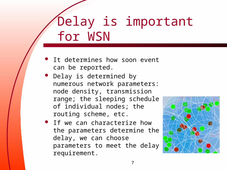
It determines how soon event can be reported.
Delay is determined by numerous network parameters: node density, transmission range; the sleeping schedule of individual nodes; the routing scheme, etc.
If we can characterize how the parameters determine the delay, we can choose parameters to meet the delay requirement.

Outline
IntroductionDelay analysis
– Hop count analysis One –dimensional Two –dimensional
– Source – destination delay analysis Random source –destination Delay from multi-source to sink
– Flat architecture– Two-tier architecture
Conclusion

Our approach
Firstly, we try to characterize how network parameters such as node density, transmission range determine the hop count;
Then we consider typical traffic patterns in WSN, and then characterize the delay.
Random source to random destinationData aggregation in two-tier clustering architecture

Outline
IntroductionDelay analysis
– Hop count analysis One –dimensional Two –dimensional
– Source – destination delay analysis Random source –destination Delay from multi-source to sink
– Flat architecture– Two-tier architecture
Conclusion
Modeling
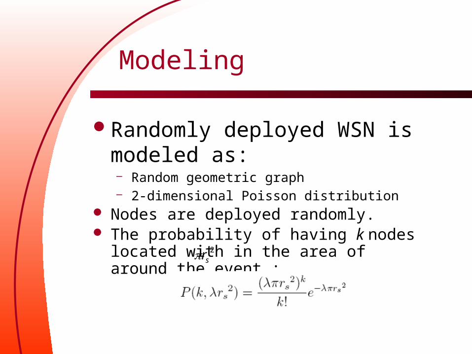
Randomly deployed WSN is modeled as:– Random geometric graph– 2-dimensional Poisson distribution
Nodes are deployed randomly. The probability of having k nodes located with in
the area of around the event :2sr
12
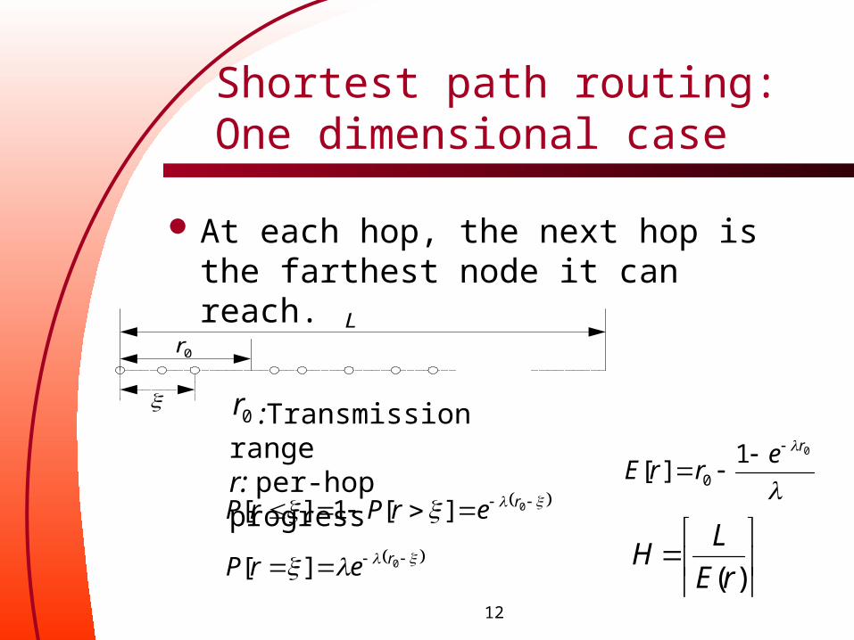
Shortest path routing: One dimensional case
At each hop, the next hop is the farthest node it can reach.
0rL
0][1][ rerPrP
0][ rerP
01][ 0
rerrE
:Transmission ranger: per-hop progress
)(rE
LH
0r

Two-dimensional case
Per-hop progress
0r
1r
1
2
2r

14/50
Average per-hop progress in 2-D case
220][1][ rePP
2202][ reP
0 0
0
cos][
][
r
ddrP
rE
Average per-hop progress as node density increases

15
Numeric and simulation results
Hop count between fixed S/D distance under various transmission rangeIt shows that our
analysis can provide a better approximation on hop count than .
0r

Hop count simulations
Hop count between various S/D distanceIt shows that our analysis can provide a better approximation on hop count than .
r

Outline
IntroductionDelay analysis
– Hop count analysis One –dimensional Two –dimensional
– Source – destination delay analysis Random source –destination Delay from multi-source to sink
– Flat architecture– Two-tier architecture
Conclusion

Per-hop delay and H hop delay
In un-coordinated WSN, per-hop delay is a random variable between 0 and the sleeping interval (Ts).
Per-hop delay is denoted by d:
2)( sT
dE
sT
s
s
Tds
TdEsd
0
22
12
1)]([)(

19
Random source/dest traffic
Hop count between random S/D pairs
22
2
4)(
22
4/
LLL
P DS
Distance distribution between random S/D pairs in a square area of L*L:

Heterogeneous WSN
Sensor nodes might have different capabilities in sensing and wireless transmission.
http://intel-research.net/berkeley/features/tiny_db.asp

21
Random deployment of heterogeneous WSN
N1 = 100N2 = 300L = 1000m
22/50
Modeling
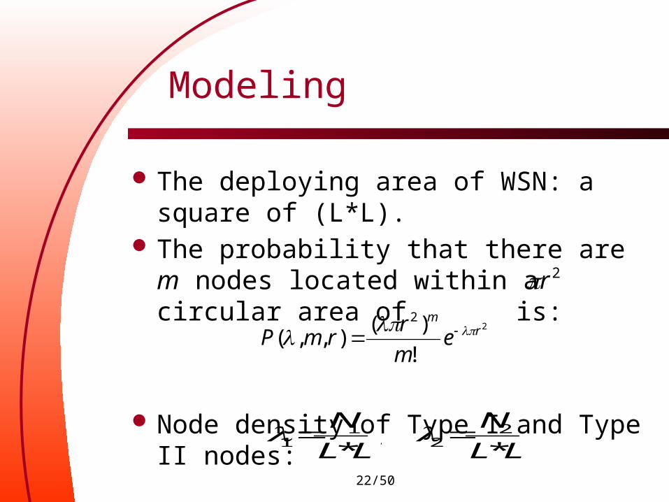
The deploying area of WSN: a square of (L*L).
The probability that there are m nodes located within a circular area of is:
Node density of Type I and Type II nodes:
,*
11 LL
N
LL
N
*2
2
2
!
)(),,(
2r
m
em
rrmP
2r
23
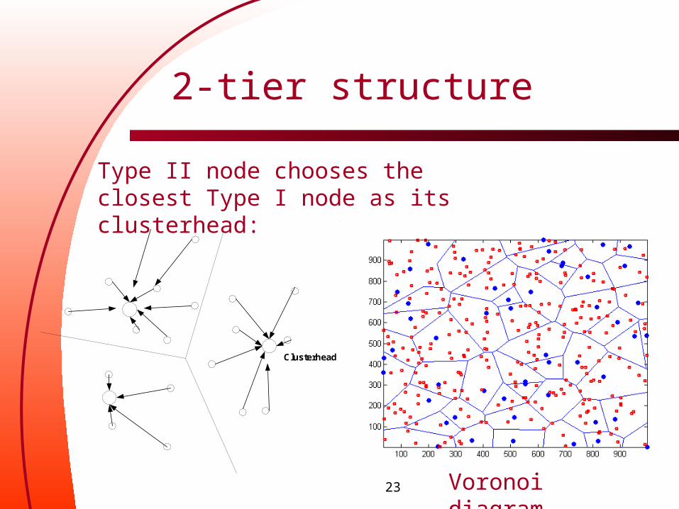
2-tier structure
Clusterhead
Type II node chooses the closest Type I node as its clusterhead:
Voronoi diagram

24/50
Distance distribution
PDF of the distance to from Type II sensor node to its clusterhead
21
12)( evP
Distance distribution between a Type II sensor node to its closest Type I sensor node:
1
2)(
vE
Average distance:

25
Average delay in 2-tier WSN
120
2
0 20
),,(
),,()(
2
|)(
rF
T
dvrF
vvP
T
hHdEEDE
s
Ls
Average delay:
Per-hop progress

26/50
Summary on delay analysis
The relationship between node density, transmission range and hop count is obtained.
Per-hop delay is modeled as a random variable.
Delay properties are obtained for both flat and clustering architecture.
27/50
Conclusion
Analysis delay property in WSN;It covers typical traffic patterns in
WSN;The work can provide insights on
WSN design.
28
Thanks.
Questions?

29
Random source to central sink node
Laptop computer

30
Incremental aggregation tree

31
Hop count analysis (Key assumptions)