delay modeling and long-range predictive control of
TRANSCRIPT

University of Central Florida University of Central Florida
STARS STARS
Electronic Theses and Dissertations, 2004-2019
2009
Delay Modeling And Long-range Predictive Control Of Czochralski Delay Modeling And Long-range Predictive Control Of Czochralski
Growth Process Growth Process
Dhaval Shah University of Central Florida
Part of the Electrical and Electronics Commons
Find similar works at: https://stars.library.ucf.edu/etd
University of Central Florida Libraries http://library.ucf.edu
This Doctoral Dissertation (Open Access) is brought to you for free and open access by STARS. It has been accepted
for inclusion in Electronic Theses and Dissertations, 2004-2019 by an authorized administrator of STARS. For more
information, please contact [email protected].
STARS Citation STARS Citation Shah, Dhaval, "Delay Modeling And Long-range Predictive Control Of Czochralski Growth Process" (2009). Electronic Theses and Dissertations, 2004-2019. 4012. https://stars.library.ucf.edu/etd/4012

DELAY MODELING AND LONG-RANGE PREDICTIVE CONTROL OF CZOCHRALSKI GROWTH PROCESS
by
DHAVAL SURESH SHAH B.S. Maharaja Sayajirao University of Baroda, India, 1998
M.S. University of Central Florida, 2003
A dissertation submitted in partial fulfillment of the requirements
for the degree of Doctor of Philosophy in the School of Electrical Engineering and Computer Science
in the College of Engineering and Computer Science at the University of Central Florida
Orlando, Florida
Spring Term 2009
Major Professor: Christine Klemenz

© 2009 Dhaval Suresh Shah
ii
ABSTRACT
This work presents the Czochralski growth dynamics as time-varying delay based
model, applied to the growth of La3Ga5.5Ta0.5O14 (LGT) piezoelectric crystals.
The growth of high-quality large-diameter oxides by Czochralski technique
requires the theoretical understanding and optimization of all relevant process
parameters, growth conditions, and melts chemistry. Presently, proportional-integral-
derivative (PID) type controllers are widely accepted for constant-diameter crystal
growth by Czochralski. Such control systems, however, do not account for aspects such
as the transportation delay of the heat from crucible wall to the crystal solidification
front, heat radiated from the crucible wall above the melt surface, and varying melt level.
During crystal growth, these time delays play a dominant role, and pose a significant
challenge to the control design.
In this study, a time varying linear delay model was applied to the identification
of nonlinearities of the growth dynamics. Initial results reveled the benefits of this model
with actual growth results. These results were used to develop a long-range model
predictive control system design. Two different control techniques using long range
prediction are studied for the comparative study. Development and testing of the new
control system on real time growth system are discussed in detail. The results are
promising and suggest future work in this direction.
Other discussion about the problems during the crystal growth, optimization of
crystal growth parameters are also studied along with the control system design.
iii

To my parents, Suresh Shah and Kokilaben Shah, who have taught me the values of hard
work, discipline and sacrifices.
iv

ACKNOWLEDGMENTS
I would like to express my gratitude to all those who gave me the possibility to
complete this work.
First, I would like to thank the Department of Electrical Engineering and
Computer Sciences (EECS) of the University of Central Florida (UCF) for providing me
support throughout my studies. Then, I would like to express my thanks to Dr. C.
Klemenz, whose continuous encouragements and support have allowed me to perform
and complete this work. During my studies, I have learned many important lessons not
only in the area crystal growth but also for life from her. In particular, I can mention
simplicity, hard work and optimistic attitude. I am glad that I could work in a field where
I could really apply my understanding of the area of controls, and at the same time learn
and contribute to advances in a field, crystal growth, so important for technological
applications.
In addition, I would like to thank Dr. Malocha, Dr. Haralambous, Dr. Dhere and
Dr. Schoenfeld, who served on my thesis committee and provided their support. Their
comments were very helpful to the performance and improvement of this study.
I cannot thank enough to my parents, my brother and my wife, whose
encouragements and sacrifices kept me focused during my study.
v

TABLE OF CONTENTS
LIST OF FIGURES ............................................................................................................ x
LIST OF TABLES........................................................................................................... xiv
CHAPTER 1: INTRODUCTION....................................................................................... 1
1.1 Problem statement and objective .............................................................................. 1
1.2 Time delay system introduction................................................................................ 4
1.3 Long range predictive control................................................................................... 9
1.4 General outline.......................................................................................................... 9
CHAPTER 2: CZOCHRALSKI GROWTH FUNDAMENTALS................................... 11
2.1 Introduction to Czochralski growth process ........................................................... 11
2.2 Crystal structure ...................................................................................................... 14
2.3 Linear dynamics of the Czochralski growth ........................................................... 17
2.3.1 Meniscus dynamics.......................................................................................... 19
2.3.2 Effect of base temperature to the crystal radius............................................... 20
2.3.3 Effect of power on the base temperature ......................................................... 22
2.3.4 Dynamic relation of radius to weight............................................................... 23
2.3.5 Time delay model ............................................................................................ 25
2.4 Literature review: crystal growth process............................................................... 26
2.5 Cascade controller structure.................................................................................... 29
2.6 Parameter measurement .......................................................................................... 31
CHAPTER 3: LONG-RANGE PREDICTIVE CONTROL............................................. 33
3.1 General introduction to long range prediction control............................................ 33
3.2 The recursive least square technique ...................................................................... 34
vi

3.2.1 Process model identification fundamentals ..................................................... 34
3.2.2 Recursive least square error technique ............................................................ 36
3.3 Introduction to long range predictive control ......................................................... 37
3.3.1 Long range predictive control technique ......................................................... 37
3.3.2 Design parameter for LRPC technique ............................................................ 43
3.3.3 Constraints ....................................................................................................... 44
CHAPTER 4: SYSTEM STRUCTURE AND MOTIVATION....................................... 46
4.1 System structure and control parameter.................................................................. 46
4.1.1 Furnace structure and instrumentation............................................................. 46
4.1.2 Present control system of Czochralski growth................................................. 48
4.1.3 Calculation of growth rate from weight signal ................................................ 49
4.1.4 Growth rate set point for cone and cylindrical part ......................................... 50
4.2 Time delay modeling of Czochralski growth process............................................. 53
4.2.1 Experimental setup........................................................................................... 54
4.2.2 Crystal growth at constant power .................................................................... 57
4.2.3 Impulse test and step test for Crystal-1............................................................ 59
4.2.4 Step test for Crystal-1 ...................................................................................... 61
4.2.5 Sinusoidal test for Crystal-2 and Crystal-3...................................................... 63
4.2.6 Offline model identification based on ARMA model...................................... 68
4.3 Initial results and motivation .................................................................................. 70
CHAPTER 5: DEVELOPMENT OF CONTORL SYSTEM........................................... 72
5.1 New controller structure ......................................................................................... 72
5.1.1 Specifications and assumptions ....................................................................... 72
vii

5.1.2 New model of the controller ............................................................................ 74
5.1.3 Flow chart of the control software ................................................................... 76
5.1.4 Operation modes .............................................................................................. 79
5.1.5 Process parameters for measurement, control and calculation ........................ 82
5.1.6 Development of the graphical user interface and LabVIEW software ............ 85
5.1.7 Method of operation for the operator............................................................... 87
5.2 Initial parameters for new controller....................................................................... 89
5.2.1 Common problems during crystal growth ....................................................... 89
5.2.2 Input-output and set point calculations for control .......................................... 93
5.2.3 Process model for identification and prediction .............................................. 96
5.2.4 Data accumulation for model identification .................................................. 100
5.2.5 Calculating set point trajectory ...................................................................... 102
5.2.6 Process simulation and offline tuning............................................................ 104
5.3 Instability and model identification ...................................................................... 106
5.3.1 Results and analysis for Crystal-4 and Crystal-5........................................... 109
5.3.2 Predefined model for long range predictive control ...................................... 113
CHAPTER 6: IMPLEMENTATION OF LRPC CONTROL ........................................ 117
6.1 Modified control model ........................................................................................ 117
6.2 Long range predictive PID control and crystal growth......................................... 120
6.2.1 Introduction of PID control............................................................................ 120
6.2.2 Crystal-6 growth by LRPC-PID..................................................................... 121
6.2.3 Crystal-7 growth by LRPC-PID..................................................................... 125
6.2.4 Crystal-8 growth by LRPC-PID..................................................................... 129
viii
6.3 Long range predictive MPC control and crystal growth....................................... 134
6.3.1 Crystal-9 growth by LRPC-MPC................................................................... 134
6.3.2 Crystal-10 growth by LRPC-MPC ................................................................ 138
6.3.3 Crystal-11 growth by LRPC-MPC ................................................................ 143
6.3.4 Crystal-12 growth by LRPC-MPC ................................................................ 146
CHAPTER 7: CONCLUSION ....................................................................................... 154
7.1 Conclusion ............................................................................................................ 154
7.2 Future work........................................................................................................... 156
APPENDIX-A: ELECTRICAL AND INSTRUMENTATION DETAILS ................... 159
APPENDIX-B: ALGORITHEM FOR LRPC MPC TECHNIQUE ............................... 163
REFRENCES.................................................................................................................. 165
ix

LIST OF FIGURES
Figure 1-1: Matlab-Simulink model for transport delay..................................................... 6
Figure 1-2: Models output for simulink models ................................................................. 7
Figure 2-1: Typical crystal growth chamber at CGEL lab ............................................... 12
Figure 2-2: Complete Czochralski growth process........................................................... 13
Figure 2-3: Abnormality during seeding........................................................................... 15
Figure 2-4: Crystal geometry ............................................................................................ 16
Figure 2-5: Typical heat transfer during the Czochralski growth..................................... 17
Figure 2-6: Schematic representation of meniscus at the growth interface ...................... 20
Figure 2-7: Cascade control structure ............................................................................... 30
Figure 3-1: Comparison between STC and LRPC technique ........................................... 34
Figure 3-2: The structure of LRPC technique................................................................... 38
Figure 4-1: Control and Instrumentation diagram ............................................................ 47
Figure 4-2: Model reference adaptive control in cascade structure.................................. 49
Figure 4-3: Effect of sudden cooling on the melt ............................................................. 51
Figure 4-4: Set point of radius for cone growth................................................................ 52
Figure 4-5: Interface shape for LGT crystals.................................................................... 55
Figure 4-6: A: Impulse response; B: Step response; C: Sinusoidal response ................... 56
Figure 4-7: Effect of melt level drop on power requirement ........................................... 58
Figure 4-8: Diameter vs. melt level for constant power growth ....................................... 58
Figure 4-9: Impulse test on Crystal-1 ............................................................................... 60
Figure 4-10: Step test on Crystal-1 ................................................................................... 62

Figure 4-11: Sinusoidal response for Crystal-2 ................................................................ 63
Figure 4-12: Sinusoidal response for Crystal-3 ................................................................ 64
Figure 4-13: Time delay for Crystal-2 at 4th peak ............................................................ 65
Figure 4-14: Time delay for Crystal-2 at 5th zero ............................................................. 66
Figure 4-15: Time delay vs. % melt drop and % crystal size ........................................... 68
Figure 5-1: Proposed controller structure ......................................................................... 74
Figure 5-2: Flow chart for control program and user interface ........................................ 77
Figure 5-3: Input data: for starting the program, heating cycle and automatic growth .... 83
Figure 5-4: Various measurements, calculations and control parameters ........................ 84
Figure 5-5: Graphical user interface of LabVIEW control program ................................ 86
Figure 5-6: Generator set point calculation from the growth control feedback................ 87
Figure 5-7: Result of power failure during the growth ..................................................... 91
Figure 5-8: Cooling water and chilled water temperature fluctuations ............................ 92
Figure 5-9: Diameter error due to weighing system noise................................................ 93
Figure 5-10: Unit-less input-output of the model and set point........................................ 95
Figure 5-11: Calculation of for LRPC control ...................................................... 95 ( )u k∆
Figure 5-12: Order of delay and model for crystal growth............................................... 96
Figure 5-13: Gain scheduling for multiple model LRPC technique ................................. 99
Figure 5-14: Calculation of trajectory from the set point ............................................... 103
Figure 5-15: Block diagram of the crystal growth model for simulation ....................... 105
Figure 5-16: Crystal-4 grown with model identification ................................................ 107
Figure 5-17: Crystal-5 grown with model identification ................................................ 108
Figure 5-18: Diameter and power change graph for Crystal-4 ....................................... 109
xi

Figure 5-19: Instability in diameter and power change graph for Crystal-4................... 110
Figure 5-20: Diameter and power change graph for Crystal-5 ....................................... 112
Figure 5-21: Instability in diameter and power change graph for Crystal-5................... 112
Figure 5-22: Step response of stable model.................................................................... 114
Figure 5-23: Time response parametric data for the model ............................................ 115
Figure 5-24: Magnitude: bode plot for the derived model.............................................. 115
Figure 5-25: Phase: bode plot for the derived model...................................................... 116
Figure 6-1: Gain and delay mapping and controller parameter ...................................... 118
Figure 6-2: Crystal-6 growth by LRPC-PID................................................................... 122
Figure 6-3: Diameter and power change graph for Crystal-6 ......................................... 124
Figure 6-4: Crystal length and melt level graph for Crystal-6........................................ 124
Figure 6-5: Crystal-7 growth by LRPC-PID................................................................... 125
Figure 6-6: Diameter and power change graph for Crystal-7 ......................................... 128
Figure 6-7: Crystal length and melt level graph for Crystal-7........................................ 128
Figure 6-8: Crystal-8 growth by LRPC-PID................................................................... 129
Figure 6-9: Diameter and power change graph for Crystal-8 ......................................... 132
Figure 6-10: Crystal length and melt level graph for Crystal-8...................................... 132
Figure 6-11: Effect of weighing mechanism error on the control system ...................... 133
Figure 6-12: Crystal-9 growth by LRPC-MPC............................................................... 135
Figure 6-13: Diameter and power change graph for Crystal-9 ....................................... 137
Figure 6-14: Crystal length and melt level graph for Crystal-9...................................... 138
Figure 6-15: Crystal-10 growth by LRPC-MPC............................................................. 140
Figure 6-16: Diameter and power change graph for Crystal-10 ..................................... 142
xii
Figure 6-17: Crystal length and melt level graph for Crystal-10.................................... 142
Figure 6-18: Crystal-11 growth by LRPC-MPC............................................................. 144
Figure 6-19: Diameter and power change graph for Crystal-11 ..................................... 145
Figure 6-20: Crystal length and melt level graph for Crystal-11.................................... 146
Figure 6-21: Crystal-12 growth by LRPC-MPC............................................................. 148
Figure 6-22: Diameter and power change graph for Crystal-12 ..................................... 151
Figure 6-23: Diameter and power change graph for Crystal-12 at t=3750 min.............. 152
Figure 6-24: Crystal length and melt level graph for Crystal-12.................................... 152
xiii

LIST OF TABLES
Table 4-1: Time delay, melt level and crystal size Crystal-2 ........................................... 67
Table 4-2: Stability of the ARMA model identification................................................... 69
Table 5-1: Computation time for different model............................................................. 97
Table 5-2: Growth parameter for Crystal-4 .................................................................... 107
Table 5-3: Growth parameter for Crystal-5 .................................................................... 108
Table 6-1: Process parameter for Crystal-6 .................................................................... 122
Table 6-2: Process parameter for Crystal-7 .................................................................... 126
Table 6-3: Process parameter for Crystal-8 .................................................................... 130
Table 6-4: Process parameter for Crystal-9 .................................................................... 135
Table 6-5: Process parameter for Crystal-10 .................................................................. 140
Table 6-6: Process parameter for Crystal-11 .................................................................. 145
Table 6-7: Process parameter for Crystal-12 .................................................................. 149
xiv
CHAPTER 1: INTRODUCTION
In this chapter, the main objective and problem statement are first discussed.
Then, an introduction to the time delay system and predictive control is presented. The
detailed description is presented later, in the respective chapters. An outline of the
dissertation is given at the end of this chapter.
1.1 Problem statement and objective
The growth of crystals from the melt by Czochralski technique is a widely
accepted and economic method to produce bulk single crystals. In this technique, the
crystals are pulled from the melt using a seed crystal [1]. The temperature of the melt is
kept close to the melting temperature of the material [2], and the driving force for growth
is provided by the temperature gradients that exist at the growing interface. The heat from
the growing interface is removed through the crystal. The efficiency of this heat removal
process is governed by the thermal conductivity of the crystal material. The thermal
conductivity of oxides is much lower than Si or other semiconductors. Therefore, oxides
have to be pulled at a much lower rate, and this is very challenging in terms of process
control. During the growth, the crystal is rotated, which produces a very complex
hydrodynamic pattern in the melt and at the growing interface. This rotation also ensures
a more homogeneous distribution of the temperature gradient, but at the same time, it
produces localized variations of the growth rate that can lead to crystal defects such as
transverse growth bands. Only a few aspects are discussed herein, but from this already,
1

one can easily understand that the Czochralski growth process is extremely complex and
implies knowledge in a variety of fields.
The basic objective in Czochralski growth is to stabilize the growth process
thermodynamically, to produce a low defect crystal with the constant diameter. This can
be achieved by measuring the crystal weight as an output signal of the growth process,
which is then used as a feedback to control the heating power as an input signal. Among
others, the crystal quality depends on the growth stability, on the chemicals used, on the
design of the furnace, on the temperature gradients in the melt and crystal-melt interface,
and on the composition of the growth atmosphere [[3], [4], [5], [6]].
Presently, proportional-integral-derivative (PID) controllers in the double loop
cascade structure are the most implemented industrial method to control the Czochralski
growth process [[8], [9], [10], [11]]. Generally, such controllers are tuned based on the
lumped-parameter linear models of the system that neglects delayed effect and
nonlinearities. During the growth of oxide crystals, there is a time delay between the
applied input power and the output response (growth rate or diameter). The time delay is
mainly caused by the slower growth rate and the lower heat conductivity of the oxide
materials compared to the semiconductor materials [4]. This time delay, if not considered
during the control system design, can destabilize the process or create oscillations during
the crystal growth, even for small perturbations [7].
The Czochralski process is a nonlinear process, where all the process variables
and parameters are interrelated and have different time scales [1]. Therefore, there is no
true steady state as the parameters keep varying during the growth. The most common
variables that affect the growth process are the melt level and the crystal size. These are
2

continuously changing during the growth. To control such complex process, the tuning
parameters need to be adjusted during the growth by some technique. For this, the gain
scheduling algorithm is a better alternative, compared to PID controllers, because it
considers the time-varying process parameters for the tuning. However, because of the
dependence of the crystal quality on the stability of all process parameters, still a better
model of the process is needed. In particular, such model needs to be able to simulate the
time delay, and not just the time scales. This is required for the indirect control system
design.
Although the growth process is nonlinear, the nonlinear models, described by
partial differential equations, may not be applicable to real-time control systems. Finite
element method can be used to solve such equations, but it is too slow to execute for the
real-time control [3]. Nonlinear models are nevertheless helpful for the understanding of
the crystal growth process, but they have significant limitations because various
properties of the material must be known. Hence, lower order models, or reduced order
models, were also proposed [[8], [9], [10], [11]]. However, once again, such models do
not consider the time delay, which is a particularly critical parameter for the growth of
crystals that require a very slow growth rate. In order to achieve the sufficient crystal
quality (low density of defects), many oxide crystals require to be grown at very slow
pull rates, typically less than 1.5mm/h. The slower the growth rate (or pull rate), the more
challenging it becomes for the control system to provide the required stability.
When the growth rate is slow, the time delay in the heat and mass transport lead
to poor process control. This delay can be of the order of few minutes, at the early stages
of growth, and continuously changes as the growth proceeds. Besides the delay in heat
3

and mass transfer, the time delay is also introduced because of the way the growth rate is
measured.
The objective of this research was to design a versatile computer control system
that includes non-linearity and time-varying time delay, and that is optimized for the
growth of oxide crystals at very slow growth rates. An adaptive Long Range Predictive
Control (LRPC) of time-varying unknown time delay system is considered for the control
design. The Long Range Predictive Control by model predictive technique and PID were
studied for comparison. A modeling of the system drawn from the recursive root mean
square (RLS) is preferred to predict the system performance in the finite horizon with
varying time delay and gain.
1.2 Time delay system introduction
Time delay (TD) systems and their control systems are vast and active fields in
the mathematical and control research. Some of the research and review can be found in
[14]. The detailed study of the TD systems analysis, control and optimization is presented
by various authors. Here, the general significance of time delay system and representation
are given.
By definition, the time-delay (TD) systems are the systems in which time delays
exist between the inputs (control signals) to the systems and their resulting effects
(outputs) on them. This time-delay can be due to transport or measurement delays. Time-
delay occurs often in various engineering fields for example electronic, mechanical,
biological and chemical processes. In general, it represents the transport time or
4

calculation time. The mathematical representations of such processes can lead to delay-
differential equation or functional differential equations [14].
Time delay systems are a compromise between the lumped parameter systems
(described by the ordinary differential equations) and the distributed parameter systems
(described by the partial differential equations with initial, boundary conditions and
unknown parameters). Often the delay for fast acting processes can be neglected without
any considerable effect, like in the motor vehicle engine. On the other hand, some slow
processes cannot be modeled and realized without time delay, like crystal growth of
oxides. These kinds of processes are generally distributed parameter system. Identifying
exact models of these processes can be much more complicated for computational
realization in real-time control system.
For such distributed parameter system, each mass or energy storage element
provides the first order element in the model for simplicity [15]. Therefore, one can
consider a process having N first order elements in series, each having time constant
/ Nτ . The resulting transfer function can be represented as:
( )1( )
1 NN
G ss τ
=+
(1-1)
Here, s is the Laplace operator. For the distributed parameter system, such as
crystal growth, the value of N can be considered as infinite because each atom behaves
like an individual system. The simplification can be represented as a first order (or a
second order) system with pure dead time dτ and time constantτ . This system can be
described by the following equation, which is a first order time delay system.
5
( )( )
1dsKG s e
sτ
τ− ⋅=
+
(1-2)
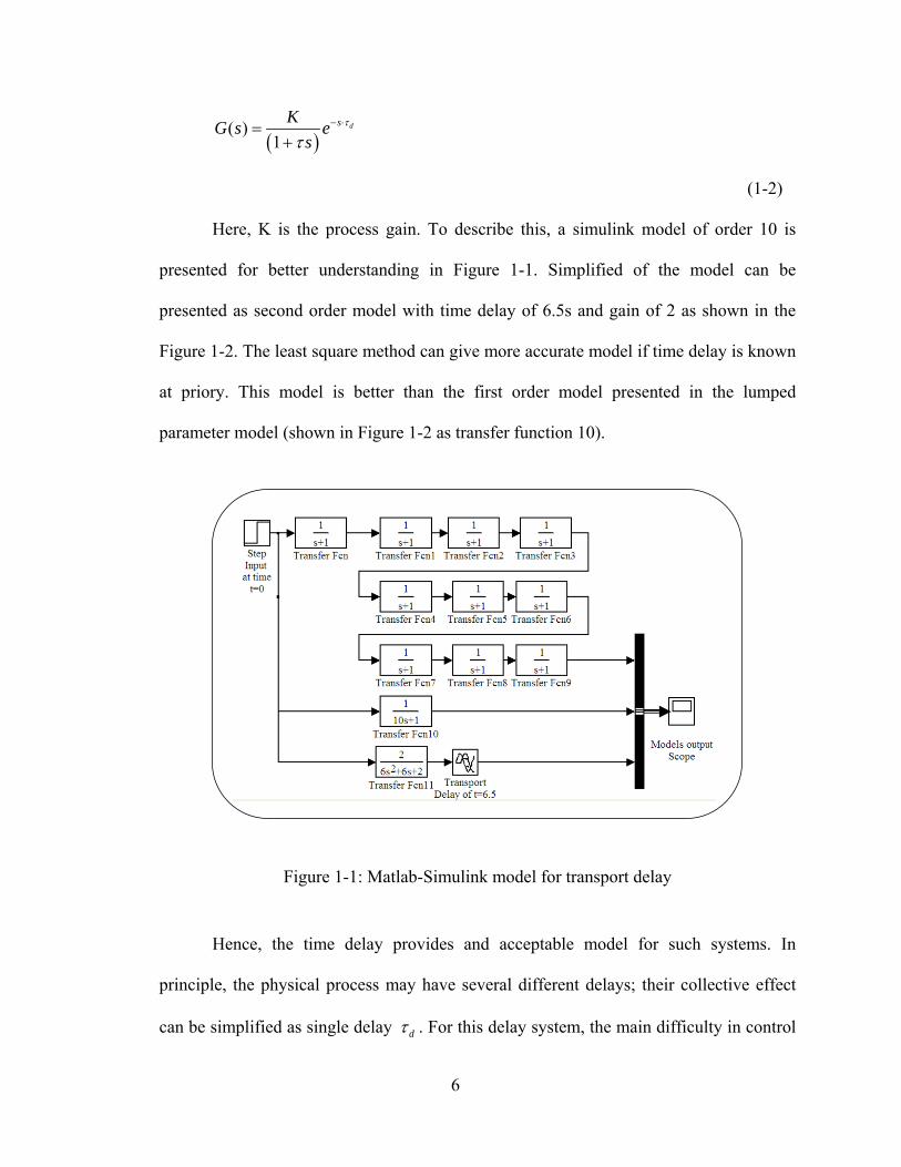
Here, K is the process gain. To describe this, a simulink model of order 10 is
presented for better understanding in Figure 1-1. Simplified of the model can be
presented as second order model with time delay of 6.5s and gain of 2 as shown in the
Figure 1-2. The least square method can give more accurate model if time delay is known
at priory. This model is better than the first order model presented in the lumped
parameter model (shown in Figure 1-2 as transfer function 10).
Figure 1-1: Matlab-Simulink model for transport delay
Hence, the time delay provides and acceptable model for such systems. In
principle, the physical process may have several different delays; their collective effect
can be simplified as single delay dτ . For this delay system, the main difficulty in control
6
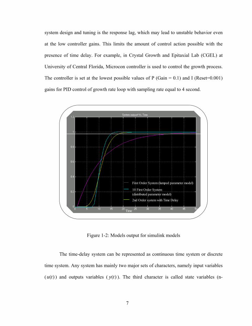
system design and tuning is the response lag, which may lead to unstable behavior even
at the low controller gains. This limits the amount of control action possible with the
presence of time delay. For example, in Crystal Growth and Epitaxial Lab (CGEL) at
University of Central Florida, Microcon controller is used to control the growth process.
The controller is set at the lowest possible values of P (Gain = 0.1) and I (Reset=0.001)
gains for PID control of growth rate loop with sampling rate equal to 4 second.
First Order System (lumped parameter model)
10 First Order System (distributed parameter model)
2nd Order system with Time Delay
Time
Figure 1-2: Models output for simulink models
The time-delay system can be represented as continuous time system or discrete
time system. Any system has mainly two major sets of characters, namely input variables
( ) and outputs variables ( ). The third character is called state variables (n-( )u t ( )y t
7

dimensional vectors at instant of time ), which represents information of the
system at time.
( )x t t
For continuous-time time delay system, the state at any time t is defined over an
interval , where depends on the delay present in the system. In other words, the
state space of continuous-time time delay system is Banach space of continuous functions
over a time-interval of length
[ , ]t t′ t′
dτ . Here, dτ is the largest time delay in the system,
mapping interval [ ,dt ]tτ− into nR . For continuous-time time delay systems, the state and
output equations in the general form can be represented as follows:
1 1( ) ( ( ), ( ), ... , ( ), ( ), ( ), ... , ( ), )d dN u uRx t f x t x t t x t t u t u t t u t t t= − − − −&
1 1( ) ( ( ), ( ), ... , ( ), ( ), ( ), ... , ( ), )d dN u uy t g x t x t t x t t u t u t t u t t t= − − − − R
(1-3)
Here, f and are nonlinear vector valued functions. Time delay periods
and represent the state and control delays in
the system, respectively. For the discrete-time time delay system, with constant sampling
period it can be represented as follows. Here, the delay is assumed to be multiple of
sampling period.
g
0, 1, 2, ... , ;dit i> = N R0, 1, 2, ... ,ujt j> =
( 1) ( ( ), ( 1), ... , ( ), ( ), ( 1), ... , ( ), )x k f x k x k x k N u k u k u t R t+ = − − − −
( 1) ( ( ), ( 1), ... , ( ), ( ), ( 1), ... , ( ), )y k g x k x k x k N u k u k u t R t+ = − − − −
(1-4)
Here, the linear discrete time time-varying delay system is considered for the
crystal growth process.
8

1.3 Long range predictive control
The model predictive control (MPC) strategy is one of the most common control
strategies is used in process industry after PID [[16], [17]]. The basic idea is to introduce
the known characteristics of the process by building a suitable model [18]. The next step
is designing a control system to minimize the required objective function by using the
error between the prediction from this model and the actual system in the predictive
horizon. The PID control action depends on past performance, but MPC control action
depends on the predictive future performance [[19], [20]].
There are many advantages of the Model predictive control over the other
methods. For example, it can be used to control various processes like long delay times,
unstable systems, non-minimum phase systems other complex processes and for the batch
process even though the process model is always varying [[16], [21]]. The predicative
control performs better for the process which has a significant delay because the future
dynamics and output of the system can be well-defined [[22], [23], [24]]. In self-tuning
control, the control signal is calculated based on the difference of the output to the
reference set point at a particular time in the future [[17], [24], [25], [26]]. However, the
Long Range Predictive Control (LRPC) is intended to control the output at set point over
a defined range of time in future. The detailed study of MPC is discussed in Chapter 3.
1.4 General outline
The first chapter was an introduction presenting the main objective of this study
and the problem statement.
9

Chapter 2 is a literature review on Czochralski crystal growth using the crystal
weighing technique. All aspects of the growth method, including the structure of the
process control system and the measurement of various parameters are presented.
Chapter 3 relates to the Long Range Predictive Control (LRPC) technique. The
general recursive least square (RLS) technique, which can be applied to identify the real-
time model of the system, is discussed. The mathematical derivation of LRPC technique
with the real-time implementation and parameter selection are also discussed. Identifying
the time delay during the real-time is left for future work.
Chapter 4 presents the work carried out in this study to model the Czochralski
crystal growth as a time delay system. The general control structure for the Czochralski
growth with the LRPC technique is presented. Results are evaluated.
Chapter 5 represents the new controller structure developed during this study. It
will discuss the software developed with LabVIEW. Real-time application related issues
are also discussed.
In Chapter 6 the result of growth experiments, carried out by using these new
control programs, are presented.
Chapter 7 is a discussion on future work, and the conclusion.
10

CHAPTER 2: CZOCHRALSKI GROWTH FUNDAMENTALS
In this chapter, a literature review of the Czochralski crystal growth process
controlled by crystal weighing technique is presented. The growth method, control
structure, and measurement of various parameters are discussed.
2.1 Introduction to Czochralski growth process
The Czochralski growth method is one of the most important melt growth
techniques used to pull single crystals from their melt [1]. The technique is widely
employed to grow single crystals of a variety of materials in different sizes ranging from
small crystal diameters of a few mm, up to crystals with very large diameters for
commercial purposes (silicon). This technique can be used for the growth of crystals over
a wide range of temperature, from low-melting compounds to very high-melting
temperature (yttrium silicate, for example) [[27], [28], [29], [30]]. The upper temperature
limit is usually set by the melting temperature of the crucible material that is used for the
growth, which is 2,400 degree Celsius for iridium. Hence, it is generally considered
relatively safe to grow (oxide) crystals up to about 2,100 degree Celsius.
The basic principle of the growth technique appears to be simple, in a first
approach, and the procedure is quite intuitive. The required amounts of chemicals are
mixed and molten in a crucible of suitable size. The crucible is placed in proper thermal
environment (insulation) in the furnace. Resistive heating or inductive heating is applied,
depending on the melting temperature of the crystal to be grown. For oxides, RF heating
is usually used. The crystals are grown from their congruent melt composition, which can
11

be different from the stoichiometric composition. The chemical preparation method may
vary with different materials and growth experiments. The size of the crucible depends on
the required crystal diameter and its length. For oxides, the crucible is made up of heavy
metal, Iridium for high-melting oxides, or platinum if a lower growth temperature can be
applied. In a typical growth experiment, the crucible containing the chemicals is heated
above the melting point of the material. The chemicals are kept molten for a while until
chemical and thermal stability are reached. Before the seeding, the temperature is reduced
progressively and manually near the melting temperature of the crystal, ideally just above
of its melting point.
Iridium Crucible
Quartz Tube
Zirconium Tube
Alumina Tube + cover
N2 gas
Zirconium Bubbles
R.F. InductionCoil
ZirconiumCeramic
N2 gas
Top Cover
Figure 2-1: Typical crystal growth chamber at CGEL lab
12

The seed is prepared with required crystal orientation, polished and etched
according to the desired growth orientation of the crystal. Normally, the seed is made up
of the same crystal grown earlier. If it not available, platinum wire or other seed can also
be used to pull a first crystal that will then be used to prepare seeds. Proper rotation rate
is adjusted for seed holding mechanism to support the meniscus at the solid-liquid
boundary. The seed is lowered and dipped vertically into the center of the melt, which is
the coldest part of the melt surface. Once the thermal stabilization is reached, the seed is
pulled out with the suitable pulling speed according to the crystal specification. Preferred
pulling speed can be different for different crystal and crystal size. Crystal growth is then
continued till required length of the crystal is achieved. Once it is pulled out the melt, the
crystal is cooled down slowly to the atmospheric temperature to avoid thermal stress.
R.F. Generator
Weighing Mechanism
Rotation Mechanism
R.F. Heating CoilPulling Mechanism
Crucible containingMelt material
Crystal
Pulling Rod
Figure 2-2: Complete Czochralski growth process
13

The heat conduction from melt to solid supports the crystallization front near the
melt-solid boundary. The temperature of the crucible and melt, thus the temperature of
the interface base, is controlled to grow the crystal of required diameter. For high
temperature growth (above 1000 degree Celsius), an RF (Radio Frequency) heating
system is used to heat up the crucible. The growth atmosphere is controlled depending on
the crystal growth under consideration. The schematic presentation of the typical crystal
growth process in the CGEL lab at UCF is shown in the Figure 2-1 and Figure 2-2.
2.2 Crystal structure
Based on the geometry of the crystal, there are mainly four crystal parts as shown
in the Figure 2-4.
• In neck growth, the diameter of the crystal is reduced. For example, seed diameter
reduced to 3mm diameter from initial 4.8 mm diameter. This early decrease helps to
lower impurity and defects propagation from the seed to the crystal [6]. This growth
is an important and difficult part of the growth. The growth process is sensitive for
any perturbation. Slight change in melt temperature can lead to seed melt (disconnect
from the melt) or sudden abnormal growth because of rapid crystallization. Therefore,
the melt temperature during the seeding has to be suitable to support the meniscus
between the melt and the crystal. During neck growth, the growth rate is in the range
of the tolerance of the weighing mechanism about ± 0.1 g/sample. For example, the
growth rate of oxide crystals is 0.1 g/h for 3 mm seed diameter. Therefore, applying
automatic control is a challenge. Generally, the operator closely observers growth
process during neck growth, which is very often done manually.
14

• During the cone growth, the crystal diameter is increased from the initial diameter to
the final required diameter. The growth rate increment depends on the half cone
angle, which represents the maximum allowable growth rate increment for the
particular crystal [30]. The power of the generator is controlled in such a way to
increase the crystal diameter. Initially, the growth rate is increased slowly. During the
middle section, the growth rate is increased rapidly. Again, at the end of the cone
growth, the growth is slowly increased for the smooth transfer to the cylinder phase.
Sharp edge near this transfer is to be avoided, as this would deteriorate the crystal
quality.
Seed MeltingAbnormal growth
Figure 2-3: Abnormality during seeding
• From application point of view, the most important phase is the cylindrical phase.
The crystal growth process runs for several days in this phase. During this phase, the
diameter of the crystal is constant and is maintained until the crystal has reached its
desired length. Also, during this phase, the thermal and fluid dynamics of the process
vary because the height of the crystal increases while the melt level decreases [[31],
[32]]. Thus, in this phase the process can be dynamically described as time-varying
15

model. The automatic control system should be adaptive with these changes [[33],
[34], [35], [36]].
Seed
Neck growth
Cone growth
Cylinder growth
End cone growth
Strong Facet
Figure 2-4: Crystal geometry
The last phase of the growth, after the crystal has reached its final length, is the
end cone growth. An end cone is required in order to avoid crystal defects that would be
generated if the crystal would be directly pulled out with its full diameter. Such defects
could then lead to the cracking of the whole crystal through their propagation from the
bottom of the crystal into its cylindrical area.
16

2.3 Linear dynamics of the Czochralski growth
The dynamics of the Czochralski growth process has been studied by various
researchers [[1], [3], [8], [11], [31]]. The growth process can be described as a time-
varying process. Nonlinear and partial differential equation based models have been
presented by various researchers, but they are only applicable to the particular crystal and
growth process used by the authors [[24], [25]]. The model developed in this work is
independent on the crystal material, and can be used, in principle, for any Czochralski
growth equipment.
To ambientqconductive
To chamber qconductive
To chamberqradiative
To ambientqradiative
To meltqconductive
To meltqconvection
To crystalqconductive
To chamber qradiative
To ambient qradiative
To ambient qconductive
To crucible qradiative
To Melt qradiative
To crystal qradiative
To crucible qradiative
To ambient qradiative + conductive
To ambientqradiativeq + conductive
To crystalqradiative
To Meltqradiative
Figure 2-5: Typical heat transfer during the Czochralski growth
17

Here, a brief review of the linear model and the stability analysis based on
perturbation analysis up to the first order is presented for further reference. A detailed
discussion on the linear model can be found in [[1], [3]].
For the high temperature crystal growth like oxide crystals, the main power input
of the process is R.F. heating source, which is controlled by suitable controller. A
crucible’s cylindrical outer surface is heated by R.F. induction from an induction coil
surrounding the growth chamber. The heat transfer during the crystal growth is mainly
driven by radiation and conduction between different parts of the chamber [3]. A typical
heat transfer mechanism from various bodies during the growth is presented in the Figure
2-5. The complete heat and mass transfer during the growth can be presented as parabolic
partial differential equation with time-varying boundary conditions and initial conditions
[[3], [34], [35]]. The simulation from these equations gives a good insight of the process
but that is not useful when applied for controlling the real-time process because of
complex computations. In addition, this simulation requires some assumptions to simplify
the simulation like infinite length of the crystal, axi-symmetry of the system and the
shape of the crystallization front. Therefore, the linear model is generally preferred to
design the automatic control system [[33], [34], [35]] for constant diameter.
During the heat transfer, heat from the crucible is transported from the crucible
walls to the crystallization interface, by conduction, radiation and convection in the melt.
At the growth interface, the heat conduction in the crystal is equal to the latent heat
generation due to crystallization of material plus heat conduction from melt to crystal [1].
This heat transfer mechanism decides the base temperature of the growth interface. The
base temperature of the interface decides the contact angle and the height of the
18

meniscus, which in turn decides the crystal diameter. Thus, this heat conduction at the
growth interface defines the meniscus dynamics. However, crystal size and diameter also
affects the interface temperature. The temperature of the crystallization base cannot be
measured during the growth. Hence, in the weighing technique, the diameter of the
crystal is estimated using the load cell or weighing mechanism [[12], [27], [28], [30]].
2.3.1 Meniscus dynamics
The crystal radius is a function of the meniscus height , contact angle ( ) cr ( )h
( )Lθ between solid-liquid and the base temperature at the solid-liquid interface .
Figure 2-6 represents a general schematic of the meniscus supported by a growing
crystal. Suppose that some perturbation in the thermal stability leads to increase in the
height of the meniscus. This leads to decrease the contact angle so that the radius of the
crystal also decreases [1]. This decrease in the radius helps to increase height further.
Thus, crystal pulling is inherently unstable process. The same is true if perturbation leads
to decrease in meniscus height. However, there is a unique meniscus height,
corresponding to a unique input power for which the crystal grows at required radius at
particular pulling speed. The material properties play an important role for deciding the
contact angle and the height of the meniscus for the particular radius. The relationship
between meniscus height, contacting angle and crystal radius can be presented as
Laplace-Young equation [1]. The detail study of the thermal and the fluid dynamics of
the process can be found in [3]. However, only the first order perturbation model is
enough to describe the model as explained in [1]. In other words, radius is not only the
( )BT
19

parameter that changes with the base temperature. Base temperature changes heat and
mass transfer at the crystallization interface.
r
0Iθ 0
Lθh
Crystal
Meniscus(growth interface)
Melt level
Figure 2-6: Schematic representation of meniscus at the growth interface
2.3.2 Effect of base temperature to the crystal radius
Using approximation of the Laplace-young model, perturbation theory,
eliminating meniscus height change and contact angle change, the effect of the base
temperature to the crystal radius can be represented by the second order transfer function
as follows:
2
0 20 0
2 00 0
0 00 0
00 0 0
002 00
( )( ) ( )
2 cos
(1 sin )cos 2
2 (1 sin )cos
c
B
L L
L
S S L L L
L
L L
L
r s CT s s As B
k G v hAh L r
v k G h k GBLr h r
k vCh L
β θ
θθ
0
β
θθ
= −+ +
= −
⎛ −= −⎜ ⎟⎜ ⎟
⎝ ⎠−
=
⎞
20

, Thermal conductivities of liquid and solid respectivelyL Sk k =
0 0, Axial temperatue gradient in liquid and solid respectivelyL SG G =
0 Axial growth rate or actual pulling speedv =
0 Initial meniscus heighth =
0 Initial radius of the crystalr =
Laplace constantβ =
0 Characterisitc material conatact angleLθ =
(2-1)
In above equation, the negative sign is due the fact that any increases in the base
temperature cause the crystal diameter to decrease eventually and vice versa.
In addition, the actual pulling speed should include the rate of change of the melt
level . ( )mh
0 p mv v h= − &
These equations are drawn according to linear perturbation theory with the
assumptions of semi-infinite crystal cylinder and the interface temperature equals to
melting temperature of the material. mT
In actual crystal growth process, change in the base temperature does not change
the radius immediately. Due to the heat conduction inside the crystal and the shape of
present interface, it takes some time (time delay) to change the radius effectively. This
time delay depends not only on crystal diameter and temperature change but also on the
length of the crystal, the crystal position in the melt, the shape of the interface and the
surrounding environment [3]. Therefore, the process can be represented as time delay, or
21

so called second order lag plus delay, in the above equation. The final radius is reached
when the heat transfer across the interface becomes stable.
2.3.3 Effect of power on the base temperature
As described earlier, the input to the process is the power supplied to the crucible
outer wall by R.F. induction coil surrounding the growth chamber. The power change
delivered to the crucible changes the melt temperature gradient, which is difficult to
measure and quantify at real-time. Generally, the melt temperature is assumed constant
and equal to the base temperature of the interface . In addition, for high temperature
growth process, the radiation is the main source of the heat transfer.
BT
From energy transfer balance equation in the melt, the transfer function of the
power supplied to the base temperature can be presented as follows:
( ) 1( ) ( )
B
h h L L
T sP s m C m C s α
=+ +
0
0
4Where, ( )h h L L
Pm C m C T
α =+
, Mass of heater (in this case it is crucible) and melt respectivelyh Lm m =
, Specific heat of the heater (crucible) and the melt respectivelyh LC C =
0 Steady state input powerP =
0 Steady state melt temperatureT =
(2-2)
Again, this equation is drawn by applying linear perturbation theory approximated
up to the first order. As the crystal grows, the melt level changes due to the mass of melt
22

Lm decreases. As a result, the process parameters keep varying. In other words, the melt
level change not only causes the melt and crucible temperature to vary, but also causes
the Eigen-structure of the model to change with time [1]. In actual process, the transport
delay of heat from crucible to the base of the meniscus has to be considered, specifically
for the oxide crystals growth, due to the large thermal capacitances within the system. In
perturbation analysis up to the first order, this delay is neglected by ignoring thermal
gradient in to the melt.
However, this delay can destabilize the process and process may oscillate if the
tight control is provided. To avoid this, the tuning parameter can be reduced by
compromising performance, which becomes sluggish. Although, this analysis is valid, in
general, up to certain temporal frequencies as described in [1] but for the oxide crystal,
unlike silicon crystal, the low thermal diffusivity can create large delay. This delay is not
negligible. This time delay depends on the melt level and flow pattern in the melt [3]. The
flow pattern can be different for the different crystal and the rotation rate. Hence, the
complete model of the crystal growth process is described as time-varying time-delay
model instead of linear time-varying system. In this study, the effect of this time delay is
considered to design proper controller structure.
The overall transfer function of the process is obtained by combining two-transfer
function equations: (2-1) and (2-2). The transfer function has three time-varying poles.
The total delay can be considered as combined delay.
2.3.4 Dynamic relation of radius to weight
Several techniques for measuring the crystal radius during the growth are
proposed and are in application today but one of the most widely accepted is the crystal
23

weighing technique or the differential weight mode technique. In this method, the weight
change of the growing crystal is measured as a measure of radius. However, the
relationship between the weight signal and the radius is little complicated and can be
drawn by force on the load cell. The force experienced by the load cell on which the pull
rod and the crystal are suspended, is comprised of four units.
The static weight of the pull-rod ( )0m g , the crystal already grown
, contribution due to the vertically resolved unit of surface tension force 2
0
t
S g r vdtρ π⎛ ⎞⎜⎝ ⎠∫ ⎟
( )γ exerted along the length of the three-phase boundary ( 02 ( )Sr θπ γ γ θ− ) and the
weight of the supported meniscus ( ). The measured force by weighing
mechanism is thus:
2Lr gπ ρ h
S2 2
0 00
( ) 2 ( )t
S p LF t m g g r v dt r gh r θρ π π ρ π γ γ= + + + − Θ∫
0 Mass of the pull rode and the crystal at instance t = 0m =
0 , = Component of the surface tension force at the three phase boudary θγ γ
, Desnsity of the solid and the melt respectivelyS Lρ ρ =
(2-3)
Again, after applying the linear perturbation theory, the transfer function for the
radius to the weight change (W , growth rate in g/h) can be presented as follows: &
2( ) 1( )
W s s sr s
η λ= + −&
( )0 0Where, 2 / ( ) / 2L c S L ah r g h 0Svη ρ γ ρ ρ ρ= + − −⎡ ⎤⎣ ⎦
24
[ ] 202 / ( ) / 2c S L Sr g h vθ θλ γ ρ ρ ρ= − −
(2-4)
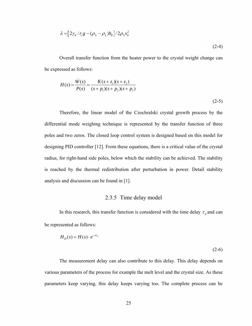
Overall transfer function from the heater power to the crystal weight change can
be expressed as follows:
1 2
1 2
( )( )( )( )( ) ( )( )( )
K s z s zW sH sP s s p s p s p
+ += =
+ + +
&
3
(2-5)
Therefore, the linear model of the Czochralski crystal growth process by the
differential mode weighing technique is represented by the transfer function of three
poles and two zeros. The closed loop control system is designed based on this model for
designing PID controller [12]. From these equations, there is a critical value of the crystal
radius, for right-hand side poles, below which the stability can be achieved. The stability
is reached by the thermal redistribution after perturbation in power. Detail stability
analysis and discussion can be found in [1].
2.3.5 Time delay model
In this research, this transfer function is considered with the time delay dτ and can
be represented as follows:
( ) ( ) dsDH s H s e τ−= ⋅
(2-6)
The measurement delay can also contribute to this delay. This delay depends on
various parameters of the process for example the melt level and the crystal size. As these
parameters keep varying, this delay keeps varying too. The complete process can be
25

described as the time-varying delay system. Therefore, the real-time identification of
such a model has to include the continuous identification of this time delay at every step
of the control action.
2.4 Literature review: crystal growth process
From literature review, it is obvious that the Czochralski growth has various
nonlinearity and uncertainties that should be considered during the control system design.
The most general and important characteristics are described as follows:
• The crystal growth process is nonlinear [[1], [3]]. In other words, altering one of the
process parameter can have both direct and indirect effect on other process
parameters as well as future parameters like the pulling speed and the rotation rate.
The simple example is a change of the heater power, which affects not only the
temperature at the base of the interface but also temperature gradient in melt, crystal
and growth environment. All these parameters contribute to decide the quality of the
crystal by defect and distribution of impurities [7].
• The crystal shape including the interface shape changes with the time [[37], [38]].
This effect is due to the changing heat transfer in the melt, crystal and changing
temperature field across the interface. The interface shape can also influence the
weight signal, which normally assumes a flat interface.
• The growth interface shape can be flat, concave or convex. There is an ideal rotation
rate for particular crystal to have flat growth interface [[15], [39], [40]]. The induced
forced convection, caused by the crystal rotation, in the melt can be a dominant effect
on the heat transfer. However, with the melt level changes this rotation rate can
26

destabilize the growth. Therefore, the rotation rate is kept well under the limit of the
ideal rotation rate for flat interface. This low rotation causes the convex shape of the
interface. In other words, crystal grows like an iceberg floating on the melt. However,
this can lead to slower measurement response due to buoyancy effect on the crystal.
In this condition, the diameter calculated from the weight change, or growth rate, is
larger than the actual diameter of the growing crystal. In oxide crystals growth, the
calculated diameter can be about 20% bigger than actual diameter.
• The power required for the constant diameter crystal growth varies with the change in
dynamics [1]. It is presented that initial power requirement is high compared to
midsection. However, at the end again, the power requirement is high, mainly due to
decreased melt to crucible contact area.
• The required power for similar diameter crystal changes with each growth due to the
change in crucible, crystal, crucible position, crystal size, growth process design and
time [[5], [6], [34]]. In other words, no two growth processes are identical even for
the same material.
• The design of the crystal growth furnace is carried out before the real growth.
Furnace structure and related parameters, like temperature gradient inside the
chamber, play a dominant role for the quality and the stability of the growth process
[[41], [42]].
• Many oxide crystals grown form the melt have low growth rates [[7], [42]]. The
longtime of stabilization of the growth parameters makes them sensitive to any
perturbation. Therefore, for the controller to be applicable for a single class of
27
crystals, it should have a structure to compensate or consider this long lag typical to
each crystal growth.
• The controller should be able to keep up with several phases of the crystal growth
process including proper cooling and heating stage. The manual to automatic change
over is necessary for control signal [36].
• The second derivative of the weight signal can be analyzed for a proper control
action. This can help to reduce the time delay or help to find out the suitable direction
for prediction of the system output [[1], [43]].
• The crucible, melt and crystal time constants are coupled with one another [9].
• Some unknown and unpredictable perturbations may arise during the growth, for
example the generation of facet plane at the interface or parallel to the growth
direction [44]. Such effects can influence the predictive value of the output. Facet
formation can sometime be controlled by adjusting the rotation rate of the crystal,
specifically in oxide crystal. Additive or dopant can also affect facet formation.
• The thermal stress on the crystal during the growth is presented as a main source of
dislocation formation and multiplication [[4], [6]]. The mathematical representation
of such a mechanism is not available to predict the generation of higher dislocation
density. However, it is obvious that the lesser the thermal stress is, the lower the
dislocation density will be. Dislocations can also propagate from the seed region into
the crystal and continue to propagate along the entire crystal length.
• The starting melt composition and the seed orientation can also influence the
Czochralski growth [5].
28
• The large size crystals are more sensitive to any perturbation than small size crystals.
Extra care has to be taken during the control design of such crystal growth [7].
• The ratio of the melt depth to the crucible height is presented as a most pronounced
effect on the thermal oscillation in the melt and the crystal [[3], [29]]. This can
change the heat transfer time from the crucible to the melt interface. The change of
the input power required for constant diameter can be related to this ratio. Other
parameters like the cooling water, the grid voltage and the frequency and the growth
atmosphere can also affect the crystal growth [[36], [43]].
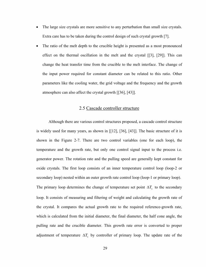
2.5 Cascade controller structure
Although there are various control structures proposed, a cascade control structure
is widely used for many years, as shown in [[12], [36], [43]]. The basic structure of it is
shown in the Figure 2-7. There are two control variables (one for each loop), the
temperature and the growth rate, but only one control signal input to the process i.e.
generator power. The rotation rate and the pulling speed are generally kept constant for
oxide crystals. The first loop consists of an inner temperature control loop (loop-2 or
secondary loop) nested within an outer growth rate control loop (loop-1 or primary loop).
The primary loop determines the change of temperature set point sT∆ to the secondary
loop. It consists of measuring and filtering of weight and calculating the growth rate of
the crystal. It compares the actual growth rate to the required reference-growth rate,
which is calculated from the initial diameter, the final diameter, the half cone angle, the
pulling rate and the crucible diameter. This growth rate error is converted to proper
adjustment of temperature sT∆ by controller of primary loop. The update rate of the
29
growth rate cycle depends on the controller structure, diameter (range of temperature
change for diameter change) and material.
Growth RateSet Point
Error = G- Gset
Weight Signal & CalculatingGrowth Rate
Crystal Growth Station
SystemTemperature
Controller( Furnace power)
Controller( Calculate Ts)
RF PowerUnit
Error = T- Ts
SecondaryLoop
PrimaryLoop
GT
Ts
Figure 2-7: Cascade control structure
Loop-2, secondary loop, mainly works for controlling the required temperature. It
measures the present temperature of the process . This temperature is compared to the
required temperature based on the loop-1 temperature adjustment and the initial
temperature . This error signal is used to create proper control signal u for the heating
unit (in this case R.F. Generator) by the controller. The generator adjusts the power based
on the control signal. Therefore, the heating of the crucible changes to adjust the required
temperature for required growth.
T
iT
The secondary loop can be fast, the control signal updates every few ms, where as
for the primary loop, control signal updates every few seconds [43]. This structure is also
good for manual to automatic changeover if manual interruption is needed [[10], [43],
30

[45]]. For example, during the initial stage of the seeding and the small diameter growth,
an operator is needed to make the manual temperature changes. During this time only
secondary loop (loop-2) is in action. In other words, Loop-1 is not adjusting any
temperature and it is open and operator changes temperature manually. This
flexibility is important for the practical implementation of the growth with out any
perturbation. However, for our growth system, we do not measure the temperature of the
growth system but we measure the power output of the R.F. generator. The current
transformer on the outgoing bus heats up the resistance depending on the current supplied
to the induction furnace. The temperature of this resistance is measured as a signal of the
output of the generator.
0sT∆ =
2.6 Parameter measurement
This section shows the basic equations for various variables, which are used to
calculate the radius, height of the crystal and growth rate of the crystal [[1], [27], [28],
[36]].
Let tδ be the time for which small amount of crystal, volume Vδ , is grown during
the cylindrical portion. Here, it is assumed that during this time the radius of the crystal
( ) and the pulling rate ( ) are constant. In addition, it is assumed that the density of
the solid is equal to the density of the liquid (
cr pv
LS ρρ = ) for simplicity of the calculation.
It is assumed that material is homogeneous and there is not enough material loss because
of vaporization during the crystal growth process. Hence, the volume gained by the
31

crystal due to pulling is 21 PV r v tδ π δ= and the volume gained by the crystal gains due to
melt drop hδ is 22 V r hδ π δ= . In addition, one can write from material balance equation:
21 2( )S LM V V R hδ ρ δ δ ρ π δ= + =
(2-7)
Where, Crucible RadiusR =
Simplifying, these three equations by removing hδ gives the change of weight in
time, i.e. growth rate for cylindrical growth is represented.
2 2 2 2
2 2 2S L P c c
PL S c
W v r R rW vt R r R
δ πρ ρ πρδ ρ ρ
= = =− −
&2
c
Rr
.
(2-8)
This equation is presented in [1].
From this, the approximate present radius of the crystal can be represented as: cr
2
2icP
W RrW v Rπρ
⋅=
+
&
&
The total height change of the crystal (or actual pulling speed) is (pulling speed +
melt level drop mH& ) as follows:
02
ti P m P
L
H H WH v H vt Rδ π−
= = + = +&
& &ρ
The present crystal size and the melt level can be obtained by integrating the
above two equations with growth time.
The above equation is for both cylindrical and cone growth for slowly growing
crystals because the effect of melt level drop due to the cone is very small compared to
melt level drop due to the crystal.
32

CHAPTER 3: LONG-RANGE PREDICTIVE CONTROL
Here, literature review of Long Range Predictive Control (LRPC) strategy is
presented. The recursive least square model identification is introduced to calculate the
model at real-time. Various parameters selection and implementation for the LRPC are
also discussed.
3.1 General introduction to long range prediction control
As described earlier in chapter 1, the LRPC technique is two steps process. First
step is to identify the process model followed by multistep cost function minimization to
identify proper control action. Here, step refers to time steps over which the cost function
is minimized as shown in following Figure 3-1. The cost function for predictive can be
single step or multistep function. Single step cost function model predictive control
(MPC) is called self-tuning control (STC). Whereas, the multistep cost functions MPC is
known as Long-range predictive controllers (LRPC) [16]. Here, the predictive horizon is
being extended over multiple steps into the future. STC can provide stable control
provided some prior assumptions about the process are satisfied. However, improper
choice of the model order and time-delay can destabilize STC [[46], [47]]. Although, the
performance of these LRPC depends on the design parameters, LRPC can provide
satisfactory control under these conditions. There are various classes of LRPC depending
on the model like pulse response, step response and generalized predictive control (GPC)
[24]. Here, GPC is considered for modeling.
33

Process ParameterEstimation
Past dataand Parameters
(delay and order)
d-step ahead
Pridiction
(Constrains on predictions)
Comutationof
control law
Single stagecost function
Future setpointw(k+d)
Control signalu(k)
O utputMeasurement
y(k)
Self -tuning control
N1 to N1+Nu
step aheadPridiction
Future setpointsw(k+N1) to w(k+N1+Nu)
LRPC control
Process ParameterEstimation
Past dataand Parameters
(delay and order)
(Constrains on predictions)
Comutationof
control law
Single stagecost function
Control signalu(k)
O utputMeasurement
y(k)
Figure 3-1: Comparison between STC and LRPC technique
3.2 The recursive least square technique
The recursive least square (RLS) model identification technique is described in
this section.
3.2.1 Process model identification fundamentals
Predicting the system performance requires mathematical modeling of the
process. Later, this prediction can be used to predict the process output, which is
compared with the required output in designing model predictive control. Steps for
identification of such model include selection of the model, calculation and validation of
the model [18]. The prior information and knowledge about the process is helpful for
34
selecting the model and model order. For real-life application, the selected model has to
incorporate noise, disturbance and error due to measurement and unidentified dynamics.
In addition, such model has to be designed to adapt with the process parameter changes
with the time.
However, the complete and exact representation of real-life process is not possible
due to many reasons. Mainly, the measured data may not be rich enough to model
required characteristics of the process. Also, the order of the input and output model for
the given process may not be known or identified; and the transport delay between input
and output may not be constant or known for modeling [[47], [48], [49]].
There are various kinds of discrete (for sampled data system) model available to
represent the process depending on the properties of the process [[50], [51]]. Widely
accepted, autoregressive integrated moving average with exogenous input (also called
controlled ARIMA (CARIMA)) model for the system with time varying delay and
parameters can be described as follows:
1 1 1( ) ( ) ( ) ( )) ( ) ( ) /(1 )1A z y k B z u k d C z e k z− − −= − + − −
1 11( ) 1 ( ) ...... ( ) a
a
nnA z a k z a k z−− −= − − −
1 10 1( ) ( ) ( ) ...... ( ) b
b
nnB z b k b k z b k z−− −= + + +
1 10 1( ) ( ) ( ) ...... ( ) c
c
nnC z c k c k z c k z−− −= + + +
(3-1)
Here, is a descrete time delay operator (z-transform operator).z
is a sampling instance.k
1 0 0Here, ( ),... ( ), ( ),... ( ), ( ),... ( ) are system parameters.a b cn n na k a k b k b k c k c k
35
( ), ( ), ( ) are controlled input, process output and noise, respectively.u k y k e k
is the minimum time delay in input and can be varying with time.d
This model can also be represented in matrix form as follows:
( ) ( ) ( ) ( )Ty k h k k e kθ= +
1 2 1 2Where, ( ) ( ) ( ) ... ( ) ( ) ( ) ... ( ) anda bn nk a k a k a k b k b k b kθ ⎡ ⎤= ⎣ ⎦
[ ] ( ) ( 1) ( 2) ... - ( ) ( ) ( 1) ... ( ) Ta bh k y k y k y k n u k d u k d u k d n= − − − − − − − − − −
(3-2)
This model is also called multiple liner regression models because the input and
the output parameters are linear [[16], [49]].
3.2.2 Recursive least square error technique
If the measurements are available from 1k m− + to sample (for last m data
sets) then CARIMA model can be represented as a linear multiple regression model.
k
( ) ( ) ( ) ( )TY k H k k kθ ξ= +
( )( ) ( )( 1) ( 1)( 1)
( ): ::
( 1) (( 1)
T
T
T
h ky k e ky k e kh k
k
y k m e k mh k m
θ
⎡ ⎤⎡ ⎤ ⎡⎢ ⎥⎢ ⎥ ⎢− −−⎢ ⎥⎢ ⎥ ⎢= +⎢ ⎥⎢ ⎥ ⎢⎢ ⎥⎢ ⎥ ⎢− + − +⎢ − + ⎥⎣ ⎦ ⎣⎣ ⎦ 1)
⎤⎥⎥⎥⎥⎦
(3-3)
The main objective of the least square technique is to select data sets to minimize
the cost function at instant. IJ thk
36

[ ] [1
2
0
1 1( , ) ( ( ) ( ) ( ))2 2
mTT
Ii
J k y k i h k i k i Y H Y H ]θ θ ξ ξ θ−
=
= − − − − = = − −∑ θ
(3-4)
The minimum value of with respect to leads to following control law :J θ
( )ˆ ˆ ˆ( 1) ( ) ( 1) ( 1) ( 1) ( )Tk k K k y k h kθ θ θ+ = + + + − + k
2
( ) ( 1)( 1)( 1) ( ) ( 1)T T
P k h kK kh k P k h kσ
++ =
⎡ ⎤+ + +⎣ ⎦
2( 1) ( ) ( 1) (TP k I K k h k P kσ⎡ ⎤+ = − +⎣ ⎦ )
) )
)
(3-5)
Here, is called the Kalman estimator gain matrix and is called
the covariance matrix represented as follows:
( 1K k + ( 1P k +
( 1) ( ) ( 1K k P k h k+ = + +
1 2( ) ( ) ( )TP k H k H k σ−
⎡ ⎤= ⎣ ⎦
3.3 Introduction to long range predictive control
Among other LRPC techniques, the Generalized Model Predictive control (GPC)
based technique considers an input output model with noise and delay [[24], [25]].
Therefore, it is suitable for real-time processes.
3.3.1 Long range predictive control technique
Most single input and output processes with noise can be explained by CARIMA
model as discussed before:
1 1 1( ) ( ) ( ) ( ) ( ) ( ) /(1 )1A z y k B z u k d C z e k z− − −= − + − −
37
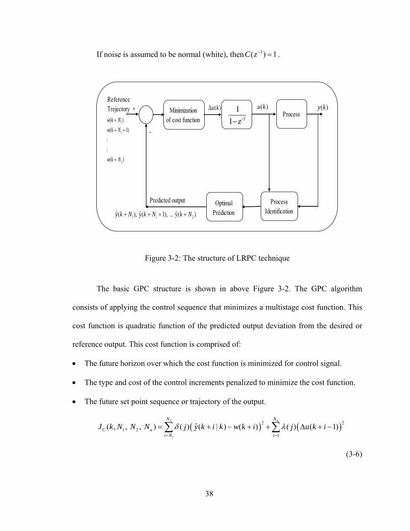
If noise is assumed to be normal (white), then 1( ) 1C z− = .
Minimization of cost function1
1
2
( )( 1)
::
( )
w k Nw k N
w k N
++ +
+
( )u k∆ ( )u kProcess
ProcessIdentification
Optimal Prediction
Reference Trejectory
1 1 2ˆ ˆ ˆ( ), y( 1), ... y( )y k N k N k N+ + + +
Predicted output
-
+ ( )y k1
11 z−−
Figure 3-2: The structure of LRPC technique
The basic GPC structure is shown in above Figure 3-2. The GPC algorithm
consists of applying the control sequence that minimizes a multistage cost function. This
cost function is quadratic function of the predicted output deviation from the desired or
reference output. This cost function is comprised of:
• The future horizon over which the cost function is minimized for control signal.
• The type and cost of the control increments penalized to minimize the cost function.
• The future set point sequence or trajectory of the output.
( ) (2
1
2 21 2
1
ˆ( , , , ) ( ) ( | ) ( ) ( ) ( 1)uNN
C ui N i
J k N N N j y k i k w k i j u k iδ λ= =
= + − + + ∆ +∑ ∑ )−
(3-6)
38

Here, is an optimum i -step ahead prediction of the system output from
the data measured up to sample . Integers are the minimum and maximum
costing horizons. Here,
ˆ( |y k i k+ )
2k 1 and N N
( ) and ( )j jδ λ
u k +
are weighting sequences for the performance.
is the future reference trajectory. The choice of this performance criterion
influences largely on the quality of the control. The control criterion can be modeled as
per required closed loop criterion of the system.
( )w k i+
The objective is to calculate the future control sequence
to drive the plant future output( ),u k ( 1), ... ( )uu k N+ 1( )y k N+ , …
to the corresponding reference trajectory
1y( 1)k N+ +
2y( )k N+ 1( )w k N+ , , …
by minimizing the control cost function . The Diophantine
equation is useful to calculate the output prediction. It is presented as:
1w( 1)k N+ +
2w( )k N+ 1 2( , , , )CJ k N N Nu
11 1 1 1 11 ( ) ( ) ( ) with ( ) ( ) and 1ii iE z A z z F z A z A z z− − − − − −= + = ∆ ∆ =% % −−
11
1 1
1 (( )( ) ( )
ii
i)z F zE z
A z A z
− −−
− −⇒ = +% %
(3-7)
The equation (3-1) is multiplied by 1( ) iiE z z−∆ , using the above equation and
simplifying; the output the prediction ˆ( ( )) y k i+ can be written as:
1 1 1 1ˆ( ) ( ) ( ) ( ) ( ) ( 1) ( ) ( )i i iy k i F z y k E z B z u k i d E z e k i− − − −+ = + ∆ + − − + +
Canceling the white noise, the best prediction of (y k i)+ can be represented as:
1 1ˆ( ) ( ) ( 1) ( ) ( ) i iy k i G z u k i d F z y k− −+ = ∆ + − − +
1 1with ( ) ( ) ( )i iG z E z B z− −= 1−
(3-8)
39

Here, the Diophantine polynomials 1( ) and ( )i i1E z F z− −
are obtained by one
divided by 1( )A z−% until the remainder of the division can be factorized as : 1( )iiz F z− −
1 1,0 ,1 ,( ) ... + a
a
ni i i i nF z f f z f z−− −= + +
1 1,0 ,1 , 1( ) ... +e i
i i i i iE z e e z z− −−= + + ( 1)− −
Similarly, for i+1:
1 11 1,0 1,1 1,( ) ... + a
a
ni i i i nF z f f z f z−− −+ + + += + +
1, , 1 ,0 1with for 0 ... 1i j i j i j af f f a j n+ + += − = −%
(3-9)
1 11 1,( ) ( ) with i
i i i i i i iE z E z e z e f− − −+ += + =1, ,0+
With above equations, 1( )iG z− can be calculated recursively:
( )1 1 1 1 1 11 1 1, ,( ) ( ) ( ) ( ) ( ) ( ) ( )i i
i i i i i i i oG z E z B z E z e z B z G z f z B z− − − − − − − −+ + += = + = + 1−
n
1
(3-10)
I.e. the first coefficient of are identical with and the
remaining coefficient is given by
j 11( )iG z−
+1( )iG z−
1 11, 1 , 1 ,( ) ( ) with 0 ... i j i j i o j bg z g z f b j− −
+ + += + =
Here, because of the dead time of sampling period, the output of the system
can only be influenced by the input signal after sampling period . Therefore, the
most suitable values of horizons can be defined by
d
d +
1 21, uN d N d N and N N= + = + = .
With this, the set of optimal output predictions can be represented by:
40
11 1
12 2
1
ˆ( 1| ) ( )( ) ( )
ˆ( 2 | ) ( 1)( ) ( )
:
ˆ( | ) ( 1)( )
d d
d d
d N d N
y k d k G u k z F y k
y k d k G u k z F y k
y k d N k G u k N z F y k
−+ +
−+ +
−+ +
+ + = ∆ +
+ + = ∆ + +
+ + = ∆ + − + ( )
Further simplification in the matrix form can lead to:
1 1( ) ( ) '( ) ( 1)Y GU F z y k G z u k GU ζ− −= + + ∆ − = +
( )( )
( )
1 00
1 21 0 01 0
1 (1 2 0 1 0 0 1
0 .. 0.. 0
and ': : : 0 :
.. ...
d
d
N NN N d N
G g zgG g g z zg g
G G
g g g G g g z g z z
+
−+
− − −− − + −
−
1)
⎡ ⎤⎡ ⎤ ⎢ ⎥⎢ ⎥ − −⎢ ⎥⎢ ⎥= = ⎢ ⎥⎢ ⎥ ⎢ ⎥⎢ ⎥ ⎢ ⎥⎣ ⎦ − − − −⎣ ⎦
11
11 2
1
( )ˆ( 1| ) ( )ˆ( 2 | ) ( 1) ( )
, , ( ): : :ˆ( | ) ( 1) ( )
d
d
d N
F zy k d k u ky k d k u k F z
Y U F z
y k d N k u k N F z
−+
−− +
−+
⎡ ⎤+ + ∆⎡ ⎤ ⎡ ⎤⎢ ⎥⎢ ⎥ ⎢ ⎥+ + ∆ + ⎢ ⎥⎢ ⎥ ⎢ ⎥= = = ⎢ ⎥⎢ ⎥ ⎢ ⎥⎢ ⎥⎢ ⎥ ⎢ ⎥+ + ∆ + − ⎢ ⎥⎣ ⎦ ⎣ ⎦ ⎣ ⎦
If all the initial conditions are zero ( ( ) 0, ( 1) 0)y k u k= ∆ − = , the free response
function ζ is also zero. If the unit step is applied at time 1k = then the free response can
be calculated recursively as
1 11 (1 ( )) ( ) ( )i iz A z B z u k d iζ ζ− −
+ = − + ∆ − +%
0with ( ) and ( ) 0 for i 0y k u k iζ = ∆ + = ≥
The objective function from the equation (3-6) can be expressed as follows:
( ) ( )T TCJ GU W GU W U Uζ ζ= + − + − + λ
[ ]( 1) ( 2) .... ( ) TW w k d w k d w k d N= + + + + + +
41

In another form:
012
T TCJ U HU U ζ= + Β +
Where, 2( )TH G G Iλ= +
2( )T W GζΒ = −
0 ( ) ( )TW Wζ ζ ζ= − −
Making the gradient of for the minimum value of (without any constraints
on the control signal) leads to the required control sequence or control vector.
CJ CJ
1 1( ) (TU H GG I G W )λ ζ− −= − Β = + −
However, the control signal required to send the process is only the first element
of vector .U
1( ) ( ) with ( ) Tu k K W K GG I Gζ λ −∆ = − = +
And the optimal control law becomes ( ) ( 1) ( )u k u k u k= − + ∆
(3-11)
In other words, if there is no error in predicted output, no further control change is
necessary. The solution of GPC involves the inversion of N N× matrix , which could
be numerically difficult to compute in real-time. For simplicity, noise considered here is
white. If noise is colored, the pre-filter can also be included in the system model.
K
Stability analysis and closed loop relationship are presented in the paper [53]. The
stability can be guaranteed if the tuning parameters ( ( ) and ( ))j jλ δ are correctly chosen.
However, it is difficult to prove the clear dependencies of these parameters on stability.
The pre-filter for input and output measurement is suggested to improve the stability at
high frequency. It also helps to improve robust stability. High frequency disturbances can
42

occur mainly because of the modeling error and immeasurable high frequency
disturbances. This filter can be modeled to make the complete control system open loop
stable.
3.3.2 Design parameter for LRPC technique
Some of the important design considerations or parameters for this control
technique are as follows [[16], [24], [25]]:
• Starting horizon , also called minimum cost horizon, should be equal to the
maximum time-delay between the input and the output. In other words, the error
before this horizon has no importance. The underestimated time delay leads
to the nonminimum-phase response of the system. Therefore, the overestimated is
always preferred but there is no reason for to be less than the time-delay.
For , the value of
1 ( )N
1(N d> )
1N
1 N d< λ has to be such that the matrix ( ) GG Iλ+ is invertible
because first rows till 1N d= of the matrix G are zero.
• Length of the horizon 2 1(N N N ) = − should be long enough to include the rise time
of the process. For the non-minimum phase system, it has to be longer until the
process output gives positive response with the control signal.
• Length of the control horizon defines the region where the process should reach
required output. After this region the control action is zero, i.e.
uN
( 1) 0 for .uu k j j N∆ + − = >
• Generally , so that the matrix G has full rank and the inverse of uN N=
(GG I ) λ+ exists.
43

• The weighting coefficients ( ) and ( )j jδ λ are sequences that consider future
behavior. These values can be constant or exponential along the horizon. These
values can be used to tune control for particular process.
• The reference trajectory or set point sequence is used for some systems. In the
crystal growth process, the reference trajectory can be represented the required
diameter of the crystal. However, the reference trajectory does not necessarily have to
be the real reference
( ) w k
(r k i)+ . It is normally the smoothed or the low-passed filtered
set point.
( ) ( 1) (1 ) ( ) >0w k i w k i r k iα α α+ = + − + − +
• In other words, auxiliary output can be derived from the set point, which is equivalent
to placing the closed loop pole by selecting the proper function 1 ( )z−Ψ .
1( ) ( ) ( )k z y kψ −= Ψ
3.3.3 Constraints
The real-time process has some range for measurement and output. The controller
discussed above has unlimited range, which is not possible for actual process. Sensors
and actuators have limited ranges and slew rates (sometime have dead time).
Economically, also, there are some constraints that have to be considered during the
design of control, like range and speed, for the product is quality. For example, similar to
other batch processes in crystal growth, most of the quality of the crystal requires some of
the variables, like rate of change of temperature and diameter, to be under specified
limits. Violating this may cause crystal meltdown or defects generation. Control systems,
44

especially Long Range Predictive Control, used for longtime delay system, are more
prone for constraints violations and proper correction has to be considered.
Application and optimization of these constraints depends on the process that will
be attended to during the actual control system design [[16], [22], [23], [51]].
Some of the most common constraints are explained here.
• Band limited constraints: The controlled parameters have to follow the required
output within some band and can be represented as ( ) ( ) ( )y k y k y k≤ ≤ .
• Input constraints: The input or control signals have magnitude limits and can be
expressed as ( ) ( ) ( )U k u k U k≤ ≤ .
• Slew rate constraints: The control signal can only increase or decrease with certain
speed due to mechanical or other limitations and can be represented as
( ) ( ) ( 1) ( )u k u k u k u k≤ − − ≤
• There can be other constraints on the process like overshoot constraints, monotonic
behavior, nonminimum phase, actuator nonlinearities.
Handling such constrains during the control system design is complicated and
computationally challenging. The main challenge introducing these constraints in control
action and find out the control signal that can also minimizes the cost function.
In this work, these constraints and their application for the crystal growth process is
considered for control. The main challenge is real-time implementation of such
constraints on the control signal. Constraint reduction, feasibility and management also
have to be studied to further improve the control system.
45

CHAPTER 4: SYSTEM STRUCTURE AND MOTIVATION
This chapter is divided into two sections. First is system parameter, which
represents the present control related structure. The second part presents the initial
research and results carried out with this structure to study the time delay and model
identification of Czochralski growth process.
4.1 System structure and control parameter
This section is mainly focused on the present growth system structure and growth
parameters.
4.1.1 Furnace structure and instrumentation
The complete furnace structure is typical and includes power unit, growth
chamber, motors and controller units as shown in Figure 2-2.
• A 10 KHz, 50KW AC power generator provides controlled induction heating to the
crucible. The controller unit controls the generator power. The generator power
output is measured by a thermocouple, which measures the temperature of a load
resister. The current transformer, connected at generator output side, powers this
resistance. In other words, the thermocouple temperature is a measure of the power
delivered to the furnace.
• The rotation motor and pulling motors are adjusted according to the required
specification before the growth starts. Both motors are servomotors and powered by
servo controllers.
46

• A digital scale measures the weight of the growing crystal. The digital weight signal
is transferred by a serial link to the computer. The maximum weight limit for this unit
is 5 Kg with the tolerance of ± 0.1 g.
Computer
ISA Bus
AT-MIO-16E-2
AIAODIDO68 Pin Connector
AIAODIDO68 Pin Connector
AI
SCXI-1180SCXI-130250-pin Connector
SCXI-11214 thermocouple and one tyristor
SCXI-1328
AO
DI
DO
GeneratorControl
Spare
Thermocouples
Tyristor
Spare
Figure 4-1: Control and Instrumentation diagram
Presently, there are two control systems used during the crystal growth in the
Laboratory. The first one has a Quick Basic program that computes growth rate from last
300-filtered weight signals. The corresponding growth signal is converted to analog
signal. The MicRicon controller reads this signal and compares to the set point,
programmed as per requirement. Double loop cascade PID control algorithm is used to
control the generator output as discussed earlier. There are mainly two drawbacks of this
control structure. The gain and reset of the PI controllers are set at the lowest possible
47

values and tuning these PI values is not possible during the growth. Therefore, the
controller response is sluggish against disturbances.
The other system is having similar control structure. However, model reference
adaptive controller (MRAC) is designed to control the growth system instead of PID. The
reference models for the controllers are optimized during the controller design. The
exponential decaying is used for controlling crystal growth loop to compensate the
delayed effect. The complete control structure is described in [45]. LABVIEW program
with various National Instrument cards are used to design the controller unit. Control and
instrumentation diagram for this system is presented in Figure 4-1. The complete
electrical and instrumentation details are presented in APPENDIX-A. This second control
system was used to carry out initial test for modeling crystal growth system.
4.1.2 Present control system of Czochralski growth
Figure 4-2 represents present control system that was used to test the Czochralski
growth later discussed in this chapter. Typical two loop cascade structure as discussed in
Section-2.5 is controlled by Model reference adaptive control (MRAC) technique.
Every two seconds, the weight signal was measured and filtered for the growth
rate calculation. Because of the slow growth rate, the last 300 weight signals were used to
calculate the effective growth rate of the crystal and to reduce the signal to noise ratio
(which increases due to the weight differentiation) in the loop-1. The loop-1 controller
calculates the change in power at every four seconds from the error between this
measured growth rate and the required growth rate. The required growth rate is being
calculated from output of the reference crystal growth model. The loop-2 controller
controls the RF generator according to the change in power from the loop-1 feedback of
48
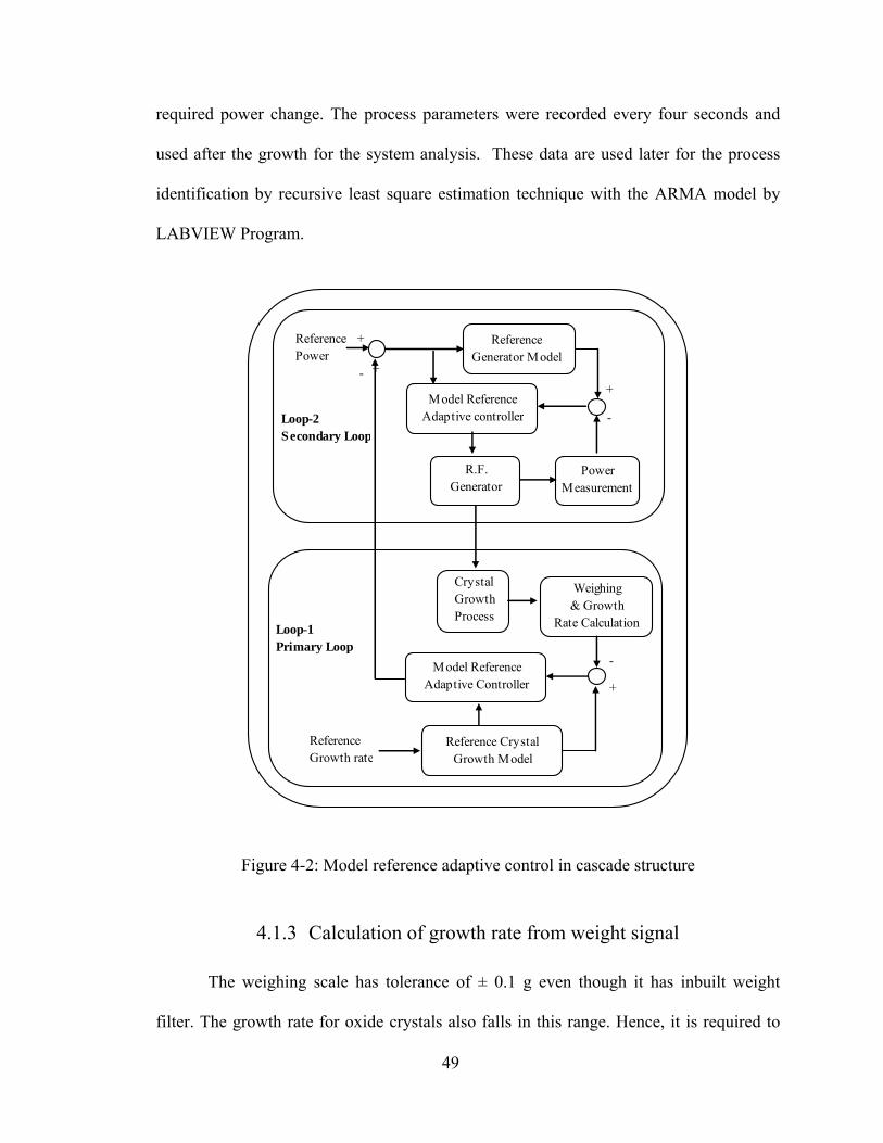
required power change. The process parameters were recorded every four seconds and
used after the growth for the system analysis. These data are used later for the process
identification by recursive least square estimation technique with the ARMA model by
LABVIEW Program.
PowerMeasurement
ReferenceGenerator Model
Loop-2 Secondary Loop
+
-
R.F.Generator
CrystalGrowthProcess
Weighing& Growth
Rate Calculation
ReferencePower
Loop-1 Primary Loop
Model Reference Adaptive controller
Reference Crystal Growth Model
Model Reference Adaptive Controller +
-
ReferenceGrowth rate
+
+-
Figure 4-2: Model reference adaptive control in cascade structure
4.1.3 Calculation of growth rate from weight signal
The weighing scale has tolerance of ± 0.1 g even though it has inbuilt weight
filter. The growth rate for oxide crystals also falls in this range. Hence, it is required to
49

filter out this noise and calculate the effective growth rate. Following digital filter reduces
the noise to ± 0.01 g.
0.5 1
1( )1
H ze z− −=
−
(4-1)
The effective growth rate is calculated from last 300 weight ( ) samples
( ) by following formula. The weight of the crystal was measured at every 4
second. In other words, the growth rate is calculated from measurements of last 20
minutes.
iW
300N =
11
6 3600. . ( 2 1)( 1)
N
N ii s
G R N i WN N N T− +
=
⎡ ⎤= ⋅ − ⋅ + ⋅ ×⎢ ⎥+ ⋅⎣ ⎦
∑
(4-2)
4.1.4 Growth rate set point for cone and cylindrical part
During cylindrical growth, required diameter of the crystal is constant. The set
point growth rate from this diameter can be calculated from Equation (2-8). To find the
ratio of the densities, we cooled down the LGT melt in the crucible by shutting off the
generator power. It created a void in the center with a small entrance on the top of the
melt surface because the melt solidified quickly near the crucible and at melt surface as
shown in following Figure 4-3. The volume of this void was measured and compared to
the melt volume. The estimated density of the melt was found to be 5.63 g/cm3. The
density of the solid material is 6.15 g/cm3. In other words, the density of the melt is about
8.5% lower than solid. These densities will be considered with Equation (2-8) to calculate
the growth rate during the cylindrical crystal growth. This is very crucial to accurately
50
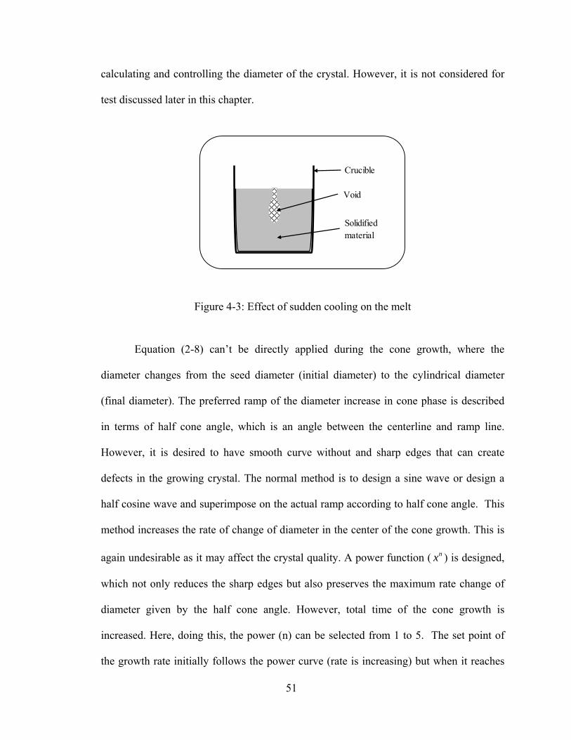
calculating and controlling the diameter of the crystal. However, it is not considered for
test discussed later in this chapter.
Void
Solidifiedmaterial
Crucible
Figure 4-3: Effect of sudden cooling on the melt
Equation (2-8) can’t be directly applied during the cone growth, where the
diameter changes from the seed diameter (initial diameter) to the cylindrical diameter
(final diameter). The preferred ramp of the diameter increase in cone phase is described
in terms of half cone angle, which is an angle between the centerline and ramp line.
However, it is desired to have smooth curve without and sharp edges that can create
defects in the growing crystal. The normal method is to design a sine wave or design a
half cosine wave and superimpose on the actual ramp according to half cone angle. This
method increases the rate of change of diameter in the center of the cone growth. This is
again undesirable as it may affect the crystal quality. A power function ( ) is designed,
which not only reduces the sharp edges but also preserves the maximum rate change of
diameter given by the half cone angle. However, total time of the cone growth is
increased. Here, doing this, the power (n) can be selected from 1 to 5. The set point of
the growth rate initially follows the power curve (rate is increasing) but when it reaches
nx
51

the maximum ramp, it will follow the straight line according to cone half angle until the
end curve (rate is decreasing). At this point, it starts following the end curve.
The calculation is carried out in three steps for the set point diameter during cone
growth as follows.
Cone Growth Calculation
0.00
0.20
0.40
0.60
0.80
1.00
1.20
1.40
0.00 5.00 10.00 15.00 20.00 25.00 30.00 35.00 40.00
Time(Hr.)
Rad
ius(
cm)
Diameter Series8
Figure 4-4: Set point of radius for cone growth
• First step is to calculate all parameters for straight-line effective radius change, slope
of the straight line, total time for the straight line and set point radius for line curve.
Effective radius change: ( er Cylindrical diamter Seed diamter) / 2= −
Slope of the straight line: ( ) tan( er pulling speed half cone angle)= ⋅&
Total time for the straight line: /line e eT r r= &
Set point of the crystal radius at time t: ( )l er t r t= ⋅&
52

• Second step is to find out the power function and related parameters.
Power function representation: ( )( ) nc liner t t T re= ⋅
Time when the power function reaches maximum slope 1nSlope linet T −= n
Total time for the cone growth: ( )11 11 2
nn n
power lineT T n n−−
− −⎡ ⎤= + −⎢ ⎥⎣ ⎦
Power function radius at Slopet t= is 1( )n
nc Slope er t r n
−−= ⋅
Line function radius at Slopet t= : 1
1( ) nl Slope er t r n
−−= ⋅
• Set point of the radius derived from above equations
For : Slopet t≤ ( ) ( ) sp cr t r t seed radius= +
For is power Slope SlopeT t t t− ≥ ≥ ( ) ( ) ( ) ( ) sp l l Slope c Sloper t r t r t r t seed radius= − + +
For : power power SlopeT t T t≥ ≥ − ( ) 1 n
powersp e
line
T tr t r seed radius
T
⎛ ⎞−⎛ ⎞⎜ ⎟= − +⎜ ⎟⎜ ⎟⎝ ⎠⎝ ⎠
For : powert T≥ ( ) spr t Cylindrical radius=
The growth rate set point is then calculated from this radius according to Equation
(2-8).
4.2 Time delay modeling of Czochralski growth process
In this study, the approach considered to model the growth process is different
from what has been commonly applied. Our approach includes the effect of system
parameters variation, and the time delay. Here, a time delay based time varying linear
model is used to model the Czochralski growth of oxide crystals at low growth rates (≤
2mm/h). This model considers the heat and mass transport delay in the process. In other
53

words, the time delay is considered as time-varying parameter as the growth advances.
The effect of the system parameters on the time delay was studied. Initially, a direct
model reference adaptive controller was employed as discussed in earlier section.
In this study, impulse perturbation and step perturbation were first applied to the
input power during the growth. Results showed a time delay between the input power
change and the output growth rate change. From these results, we derived a suitable cycle
time (reciprocal frequency) and amplitude of sinusoidal perturbations that were then
applied to the power. Results were analyzed to study the relation between the time delay
and the melt level drop. Such time delay represents not only the process delay because of
heat-mass transfer from crucible wall to the crystal interface. It also represents the phase
lag because of the weight signal and differential of the weight signal. In other words,
when the weight signal is differentiated, the controller needs a sample of hundreds of
measurements (typ. value for low growth rates) for calculating the effective growth rate.
This causes the delay due to measurement lag. Both, the process time delay and the
measurement lag, can’t be identified independently from the crystal weight change
measurements. Therefore the effective time delay observed represents the combination
both effects. Above results, not only revealed the time delay, they were also used to
identify constrains of the control, to preserve the quality of the crystal during the growth.
In particular, the tolerable limits (bounds) of the control signal and its rate of change were
determined.
4.2.1 Experimental setup
For all experiments, the crystal pulling rate and rotation rate were set at 2 mm/h,
and 32 rpm, respectively. The required diameter of the cylindrical part of the crystal was
54

33 mm. An iridium crucible of 51mm height and internal diameter was used. The
crystals were grown in nitrogen atmosphere. Various crystal growth experiments were
carried out with different rotation rate in order to achieve the optimum rotation rate for
the flat interface as shown in following figure.
Convex growthInterface withRotation rateof 40 rpm
Concave growthInterface withRotation rateof 25 rpm
Flat growthInterface withRotation rateof 32 rpm
Figure 4-5: Interface shape for LGT crystals
In all growth experiments, the crystals were first grown with automatic control up
to their cylindrical diameter. Once stable growth of a given cylindrical height was
achieved, loop-1 was stopped. From that moment on, the generator output power (Figure
4-2) was only controlled by loop-2. The first test was carried out to measure the effect of
constant power to the crystal diameter as growth proceeds and melt level drops discussed
in next section. After that, the controlled perturbations in the form of impulse, step or
55

sinusoidal were applied on the output power. Impulse test and a step response test were
carried out during the growth of Crystal-1. The sinusoidal response tests were carried out
during the growth of Crystal-2 and Crystal-3 (Figure 4-6).
A
B
C
C
Figure 4-6: A: Impulse response; B: Step response; C: Sinusoidal response
The input power supplied during seeding was used as arbitrary choice to
normalize the power change and express it in percentage. To express growth process as a
positive response system, the percentage change in power was inverted (multiplied by (-
1)). By doing this, the positive percentage of power change leads to a positive percentage
56
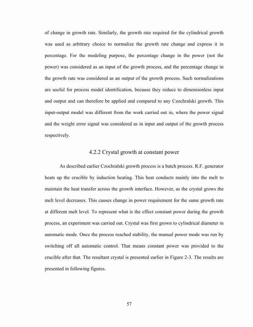
of change in growth rate. Similarly, the growth rate required for the cylindrical growth
was used as arbitrary choice to normalize the growth rate change and express it in
percentage. For the modeling purpose, the percentage change in the power (not the
power) was considered as an input of the growth process, and the percentage change in
the growth rate was considered as an output of the growth process. Such normalizations
are useful for process model identification, because they reduce to dimensionless input
and output and can therefore be applied and compared to any Czochralski growth. This
input-output model was different from the work carried out in, where the power signal
and the weight error signal was considered as in input and output of the growth process
respectively.
4.2.2 Crystal growth at constant power
As described earlier Czochralski growth process is a batch process. R.F. generator
heats up the crucible by induction heating. This heat conducts mainly into the melt to
maintain the heat transfer across the growth interface. However, as the crystal grows the
melt level decreases. This causes change in power requirement for the same growth rate
at different melt level. To represent what is the effect constant power during the growth
process, an experiment was carried out. Crystal was first grown to cylindrical diameter in
automatic mode. Once the process reached stability, the manual power mode was run by
switching off all automatic control. That means constant power was provided to the
crucible after that. The resultant crystal is presented earlier in Figure 2-3. The results are
presented in following figures.
57

Constant power response of Crystal-6
-0.6
-0.4
-0.2
0
0.2
800 1000 1200 1400 1600 1800 2000 2200
Time (minute)
% P
ower
cha
nge
-90
-60
-30
0
30
% G
row
th r
ate
chan
ge
% Temp change % Grow th rate change
Figure 4-7: Effect of melt level drop on power requirement
Constant power response of Crystal-6
30
40
50
60
70
80
90
100
5257626772778287% Melt level
% D
iam
eter
Figure 4-8: Diameter vs. melt level for constant power growth
58

From above figure, one can see that initially the diameter increases from 87%
melt level to 75% of the melt level. However, after 70% melt level, the diameter keeps
decreasing. At around 57% of the melt level crystal growth becomes unstable and
diameter decreases rapidly. From this result, one can say that initially power required for
same diameter increases but once the critical melt level reaches the power required for
same diameter growth decreases rapidly. The control structure should have adaptation as
growth proceeds.
4.2.3 Impulse test and step test for Crystal-1
The impulse test represents the relation of the output ( , the percentage
change in growth rate) with the input impulse (
( )y k
( )kδ , the percentage change in power)
applied at time in the time domain. The relation of the output to the input can be
represented as time-domain convolution integral. In discrete time domain, it is a
convolution summation and represented as follows with as the impulse transfer
function:
( )h k
( ) ( ) ( )S I
I
T T
i T
y k h k k iδ+
=
= −∑
For the non-delayed system, the initial response time is zero and the output
response of the system appears as soon as the system is exited with the input. However,
for time delayed system is not zero. In other words, the output response of the system
appears after some time. This delay is called the time delay of the system. Here, after
settling time , the input has no affect on the output and output settles at its original
value.
IT
IT
ST
59

Impulse response of Crystal-1
-2.4
-2
-1.6
-1.2
-0.8
-0.4
0
1285 1295 1305 1315 1325 1335
Time (minute)
% P
ower
cha
nge
-48
-40
-32
-24
-16
-8
0
% G
row
th ra
te c
hang
e
% Power change % Growth rate change
Figure 4-9: Impulse test on Crystal-1
In Figure 4-9, the result of the impulse response test is presented. It represents the
significant amount of time delay in the crystal growth process. Although the value of the
time delay depends on the amplitude of the impulse applied during the growth, for the
limited input power change, the time delay in the output remains bounded in some range.
Here, only 2.2% of power change was applied from 1285.87t = minute to
minute. The growth rate was decreased to about 25%. The growth rate came back to
initial state after about 50 minutes (Figure 4-6 A). The time delay and settling time was
observed to be about 6 minutes and 44 minutes respectively. These results are important
for the control system design.
1291.87t =
60

4.2.4 Step test for Crystal-1
Similarly, the step test was carried out on the Crystal-1 as shown in Figure 4-6 B
and Figure 4-10. The step response test is the first time integral of a unit impulse
occurring at the same time. In other words, in time-domain representation, a step change
in input is similar to the train of impulse occurring at each sampling time.
Therefore, the system never converges to its original state but settles to a new output
value (new growth rate). The relation of the input and the output can be described with
transfer function as follows.
( )u k
( )S k
( ) ( ) ( )Ii T
y k S k u k i∞
=
= −∑
In Figure 4-10, the result of the step response test is presented. Here, only 1% of
power change was applied at time 1538.20t = minute. The system had time delay of
about 4-minute whereas the settling time with new growth rate was about 150 minutes.
The time delay was less compared to the impulse response test because the energy
supplied (power x time) to the furnace is higher than impulse response test. Here, only
1% power change was enough to change the measured growth rate to about 75%. It
represents the importance of advanced adaptive control system during for the growth
process. Such large power change should be avoided during the actual growth. Hence, the
maximum percentage change in power has to be considered as constrain on the control to
preserve the growth stability. Also, from the Figure 4-6 B, one could see that this change
had led the generation of the defects and deterioration of crystal quality.
61

Step response of Crystal-1
-1.2
-1
-0.8
-0.6
-0.4
-0.2
0
0.2
1530 1570 1610 1650 1690
Time (minute)
% P
ower
cha
nge
-120
-100
-80
-60
-40
-20
0
20
% G
row
th ra
te c
hang
e
% Power change % Growth rate change
Figure 4-10: Step test on Crystal-1
This can also be seen in the Figure 4-10 as an abnormal increase in growth rate.
To preserve the crystal quality during the growth, the rate of change control signal (or
skew rate) during the certain period of time has to be considered as constrain on the
control signal. The value of this constraint depends on the type of crystal growth. As an
example, for LGT crystals, if grown with the similar specification, the maximum
percentage change should be less than 1% and the maximum skew rate should be as per
the half cone angle set during the cone growth. The effectiveness of such control system
will be studied later.
62

4.2.5 Sinusoidal test for Crystal-2 and Crystal-3.
The sinusoidal tests were carried out to identify the effects of system parameters,
especially the melt level and the crystal size, on the time delay during the growth of
Crystal-2 and Crystal-3. The sinusoidal perturbation in the input power was applied after
the stable cylindrical growth is reached. The sinusoidal signal had the time-varying
amplitude and the cycle time. The amplitude and the cycle time for both the sinusoidal
tests were linearly decreasing from maximum to minimum values as Figure 4-11 and
Figure 4-12. The choice of the maximum and minimum values of the amplitude and the
cycle time depend largely on the expertise of the operator and should be drawn such that
the crystal growth remains stable during the perturbation.
Sinusoidal response of Crystal-2
-0.8
-0.6
-0.4
-0.2
0
0.2
0.4
0.6
0.8
400 600 800 1000 1200 1400 1600 1800
Time (minute)
% P
ower
cha
nge
-80
-60
-40
-20
0
20
40
60
80
% G
row
th ra
te c
hang
e
Figure 4-11: Sinusoidal response for Crystal-2
63
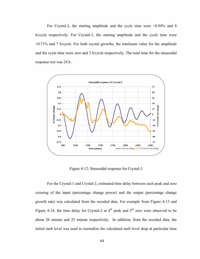
For Crystal-2, the starting amplitude and the cycle time were +0.94% and 8
h/cycle respectively. For Crystal-3, the starting amplitude and the cycle time were
+0.71% and 7 h/cycle. For both crystal growths, the minimum value for the amplitude
and the cycle time were zero and 3 h/cycle respectively. The total time for the sinusoidal
response test was 24 h.
Sinusoidal response of Crystal-3
-0.75
-0.6
-0.45
-0.3
-0.15
0
0.15
0.3
0.45
0.6
0.75
900 1100 1300 1500 1700 1900 2100 2300Time (minute)
% P
ower
cha
nge
-75
-60
-45
-30
-15
0
15
30
45
60
75
% G
row
th r
ate
chan
ge
% Power change % Growth rate change
Figure 4-12: Sinusoidal response for Crystal-3
For the Crystal-1 and Crystal-2, estimated time delay between each peak and zero
crossing of the input (percentage change power) and the output (percentage change
growth rate) was calculated from the recoded data. For example from Figure 4-13 and
Figure 4-14, the time delay for Crystal-2 at 4th peak and 5th zero were observed to be
about 26 minute and 25 minute respectively. In addition, from the recoded data, the
initial melt level was used to normalize the calculated melt level drop at particular time
64

and express it in percentage. Similarly, the final length of the crystal was used to
normalize the calculated crystal size at particular time and express it in percentage. In
Table 4-1, the percentage melt level drop, the percentage crystal size and the
corresponding time delay for each event is presented.
Sinusoidal response of Crystal-2
0.1
0.2
0.3
0.4
0.5
0.6
950 960 970 980 990 1000 1010 1020
Time (minute)
% P
ower
cha
nge
10
20
30
40
50
60
% G
row
th r
ate
chan
ge
Figure 4-13: Time delay for Crystal-2 at 4th peak
It was observed that the Crystal-2 was unstable after 6th peak and crystal diameter
was rapidly decreasing (Figure 4-11 and Figure 4-12). Therefore, data after, this peak has
not been considered for time delay analysis. The melt level drop was only from 22% to
51% during this time. For Crystal-3, due to the early disturbance during the neck growth
the crystal growth was unstable after 4th peak time. From Figure 4-12 for Crystal-3, the
time delay up to the 4th peak can be observed but due to the noise and disturbances these
data couldn’t be analyzed for the time delay.
65

Sinusoidal response of Crystal-2
-0.2
-0.1
0
0.1
0.2
1120 1130 1140 1150 1160 1170
Time (minute)
% P
ower
cha
nge
-20
-10
0
10
20
% G
row
th r
ate
chan
ge
% Power change % Growth rate change
Figure 4-14: Time delay for Crystal-2 at 5th zero
Further tests are required to observe the effect on time delay during the entire
crystal growth process. However, from Table 4-1, it is clear that the time delay varies as
the crystal growth advances. The time delay increases as the melt level drops (and crystal
size increases). In Figure 4-15, the relations are also presented by exponential trend lines.
Therefore, the time delay can be considered as a function of melt level drop for the
modeling purpose. In other words, the suitable model of Czochralski is time-varying
delay model.
66

Table 4-1: Time delay, melt level and crystal size Crystal-2
Event Melt drop Crystal size Time(%) Size (%) delay (min)
1st zero 21.98 26.24 11.731st peak 24.75 30.69 13.712nd zero 27.54 35.05 14.342 nd peak 32.01 39.87 16.063rd zero 36.32 44.58 17.273rd peak 38.47 48.05 19.974th zero 40.45 51.48 22.264th peak 43.14 55.00 26.135th zero 45.87 58.42 25.005th peak 47.70 61.33 28.486th zero 49.50 64.21 32.546th peak 51.49 66.94 32.40
The measurment of time delay for Crystal-2
Heat-mass transfer can explain such increase in time delay. As the melt level
drops, the contact area of the crucible and the melt decreases. Hence, the effective power
delivered to the melt (so to the growth interface) decreases. This effect causes the
increase in time delay. In addition, as the crystal size increases the heat conduction inside
the crystal increases. In addition, the upper part of the crystal is increasingly at a lower
temperature due to the configuration of the thermal insulation around and above the
crucible. In other words, the heat loss increases with the crystal size. Hence, the change
in power required for the appropriate change in the growth interface temperature-gradient
increases. The time required to reach stability also increases. The crystal growth response
becomes sluggish. Thus, the time delay increases because of both the melt level and
crystal size. However, any one of the parameter is enough to describe the effect on time
67

delay, as they (the melt level and the crystal size) are interrelated. One can also consider
multiplying the both parameters to model the time delay. These results are important in
designing the control system.
Crystal-2 : Time delay Vs. % Melt drop and % Crystal size
10
14
18
22
26
30
34
20 30 40 50 60 70% Melt drop and % Crystal size
Tim
e de
lay
(min
ute)
.
Time delay vs. % Melt drop Time delay vs. % Crystal size
Expon. ( Time delay vs. % Melt drop) Expon. ( Time delay vs. % Crystal size)
Figure 4-15: Time delay vs. % melt drop and % crystal size
4.2.6 Offline model identification based on ARMA model
We have presented earlier that the crystal growth process can be modeled as a
time-varying time delay system. For the advanced adaptive control system, real-time
model identification is necessary for such time-varying system. Auto regressive moving
average (ARMA) model (as shown in equation (3-1)) was considered for this
identification. Once the model parameter converges during the identification, for the
optimal control action, the objective cost function can be minimized with constrains.
Such controller is obviously advantageous compared to the conventional PID controller.
68

Here, only the stability of such process identification with higher orders model and time
delay has been checked. The main reason of considering the higher order model is that
such time varying time delay can be approximated by pade-approximation as the higher
order model with constant time delay model. The change in time delay will be
approximated by the change in parameters of higher order model during the
identification. However, the stability of such high order model needs to be studied.
Table 4-2: Stability of the ARMA model identification
Minute Model delay (d) Order 3 Order 10 Order 20 Order 30 Order 40 Order 500.00 0 0.02658 0.03026 0.05815 0.66386 17.23808 15.702022.00 30 0.03390 0.01753 0.01616 0.01494 0.02237 0.030264.00 60 0.03843 0.01759 0.01713 0.01493 0.01594 0.015496.00 90 0.04276 0.01756 0.01739 0.01493 0.01587 0.015738.00 120 0.04344 0.01755 0.01780 0.01492 0.01592 0.01557
10.00 150 0.04085 0.01761 0.01922 0.01499 0.01603 0.0155212.00 180 0.04423 0.01760 0.02115 0.01504 0.01622 0.0155914.00 210 0.06353 0.01757 0.02568 0.01504 0.01624 0.0155616.00 240 0.09364 0.01757 0.04321 0.01509 0.01624 0.0156818.00 270 0.04078 0.01752 0.09585 0.01506 0.01638 0.0157619.50 300 0.02452 0.01751 0.19463 0.01494 0.01642 0.01580
Order of the model (=A=B)Delay
For the model identification, the order of input and output were assumed to be
identical . The delay is assumed to be the multiple of sampling time. The
process model identification was carried out from the sinusoidal test results of Crystal-2
for various delays time and presented in Table 4-2. From the Table 4-2 one can see that
for and for delay range 8 minute to 18 minute, the prediction errors were
consistently lower than other models. In the other hand, for the lower order
( a bn n= ) d
30a bn n= =
69

model , the prediction errors were consistently higher. The higher order
models are better choice for model identification and prediction. According to Table 4-2,
the higher order model identification is stable in terms of predictive error,
as it remains bounded. Here, the only one step-ahead prediction error is checked.
However, during the actual control system design the prediction horizon can be extended
to cover the range of time delay, as the model is stable.
a bn n= = 3
10)( a bn n= >
4.3 Initial results and motivation
The melt level and crystal size were observed changing not only the Eigen
structure but also the time delay between the input and output during the crystal growth.
The effect is very apparent for slow growing crystals and cannot be neglected for control
system design.
The growth system considered for developing the control system is presented in
section 4.1 . Initially, the growth interface was adjusted to be flat by adjusting the rotation
rate. The instability or growth interface change occurs with the present system at around
40 to 42 rpm for LGT crystal growth. The optimum rotation rate was set to 35 rpm. The
second test was carried out to approximate the density of the melt. The fast cooling of the
melt created a void in the center of the solid material. The density of the melt was 5.63
g/cm3 calculated from the volume of the void. The density of the solid material is 6.15
g/cm3. In other words, the density of the melt is about 8.5% less. This difference will be
used during the calculation of the growth rate.
To study how the requirement of power varies for the constant diameter as growth
proceeds, a constant power test was carried out once the cylindrical diameter is achieved.
70

The result reveals that initially requirement of power increases and, as the melt level
drops below 57%, it starts decreasing. Controller has to adjust to new set point with melt
level.
Impulse test, step test and sinusoidal were also carried out to reveal the time delay and
how it changes with decreasing melt level. The results indicated an exponential relation
between melt level and time delay. The controller has to be designed to consider this time
varying delay. The constraints on the power inputs are also identified to preserve the
quality of the crystal during the growth. The real-time identification of the crystal growth
process is necessary for the predictive controller. Higher order model were proposed, as
they can be more adaptive with the time-varying delay. Stability of such model during the
off-line identification was carried out. For 30th order model, the prediction errors were
consistently lower than for the other models. However, for the lower order model the
prediction error was higher, which makes them unreliable for control. This indicates that
the higher order models were stable.
The results extracted from these experiments were useful to the design of the
controller structure discussed in the next section. The long range model predictive control
strategy along with constrain and time-delay model identification was chosen to further
design an advance controller for such slow growing crystals.
71

CHAPTER 5: DEVELOPMENT OF CONTORL SYSTEM
The objective of this study is to develop a new control system that can consider a
time- varying parameter delay and constraints. In this chapter, the new control system’s
design and development are discussed. Based on the specification, assumption and
growth requirement, the LabVIEW control program was developed. A detailed flow chart
and an operation method have been developed for the real-time growth using this
program. Initially, simulations were applied to rectify programming error, modify and
tune the program before adapting to the real-time crystal growth. Later, difficulties
related to the process model identification during real-time growth were observed. These
challenges were investigated, and suitable options to address them are presented.
5.1 New controller structure
In this section, a new controller structure is presented. At first, assumptions and
specifications for the proposed controller are briefly discussed followed by the controller
structure and the operation method.
5.1.1 Specifications and assumptions
• As shown in Equation (2-5), the continuous time transfer function of the Czochralski
crystal growth process has three poles and two zeros. However, the discrete time
function with the similar structure is not a good choice due to existence of the
unknown time delay for the slow growing crystals. The higher order model is
preferred in this work.
72

• The continuous time presentation of the time-delayed model can be presented as
follows. Here, the characteristic time delay, dτ , is total delay and can be considered
as a combined delay due to the delayed dynamics of the system and the measurement
delay.
( ) ( ) dsDH s H s e τ−= ⋅
• For simplicity, in a discrete time representation of the growth system, the time delay
is assumed as a multiple of the sampling time. Here, the order of time delay is much
greater (≥ 8 min.) than the sampling time (4 sec).
• As presented earlier, the time delay varies as the melt level or the crystal size
changes. The complete system dynamic is considered as a time varying time delay
system. However, the time delay is mainly studied here for the control system design.
• The R.F. generator transfer function is not included in the crystal growth model. In
the cascade controller structure, there is an independent controller for it. The R.F.
generator has some nonlinearities and uncertainties due to its dependence on the grid
supply. E.g., the controller should take proper action, like pulling out the crystal if
power or generator fails, in such an event.
• Generally, the output of the growth system is taken as the growth rate, which is
square function of the crystal radius. However, for the slow growing crystals, the
squared error produced by this growth rate can cause unnecessary perturbation
because of over controlled action. Instead, the calculated diameter, from this growth
rate, is considered as an output to control the growth system.
• The unit-less conversion of the power change and the diameter (input-output) should
be helpful for the model identification and the control system implementation for
73
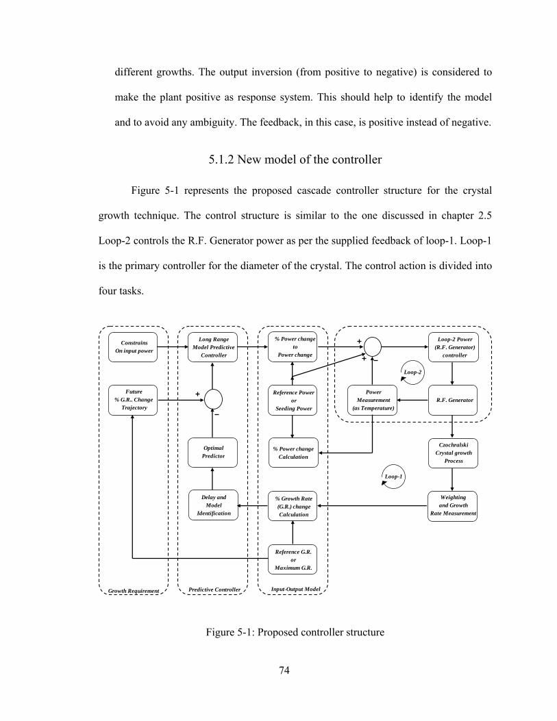
different growths. The output inversion (from positive to negative) is considered to
make the plant positive as response system. This should help to identify the model
and to avoid any ambiguity. The feedback, in this case, is positive instead of negative.
5.1.2 New model of the controller
Figure 5-1 represents the proposed cascade controller structure for the crystal
growth technique. The control structure is similar to the one discussed in chapter 2.5
Loop-2 controls the R.F. Generator power as per the supplied feedback of loop-1. Loop-1
is the primary controller for the diameter of the crystal. The control action is divided into
four tasks.
Loop-2 Power(R.F. Generator)
controller
R.F. Generator
CzochralskiCrystal growth
Process
Weighting and Growth
Rate Measurement
% Power changeto
Power change
% Power changeCalculation
% Growth Rate (G.R.) changeCalculation
Reference Poweror
Seeding Power
Power Measurement
(as Temperature)
Reference G.R.or
Maximum G.R.
Delay andModel
Identification
Long RangeModel Predictive
Controller
Future% G.R.. Change
Trajectory
Constrains On input power
Optimal Predictor
Loop-2
Loop-1
Input-Output ModelPredictive ControllerGrowth Requirement
Figure 5-1: Proposed controller structure
74

• First is a measurement task. The computer communicates with the weighing
mechanism and measures the weight of the growing crystal. The signal is then filtered
and converted into approximate growth rate and diameter of the crystal as discussed
in chapter 4.1.3. The computer control system also measures and filters the power
output of the generator in the form of the thermocouple temperature as discussed in
chapter 4.1.1.
• The second task is converting both the measurement (input of the model) and control
signal (output of the model) in percentage change form as discussed in 4.2.1. The
Calculated growth rate or the diameter will be converted in percentage growth rate or
percentage diameter change respectively. The control signal is derived from the
controller output in the percentage power change form. This control signal is a
feedback to loop-2. Here, this feedback will be positive because of the inversion in
the modeling as shown in the Figure 5-1.
• The third task involves identification of the model and deriving a control signal. Here,
the identified model is used to predict the output of the process for the control horizon
based on the delay. This predicted output is compared with the required output
(trajectory) of the growth system. The proper controller action is derived using a long
range predictive control technique.
• The forth task is to define the growth requirement (or trajectory) and future
percentage diameter change (growth rate change) trajectory. Constraints on the set
point and control signal are defined in this block.
75

5.1.3 Flow chart of the control software
Based on the new controller structure, the LABVIEW software was used in order
to develop the controller program. Figure 5-2 shows the general flow chart of the
complete control software. The program consists of not only the controller structure as
described above but also the graphical user interface (GUI), where the operator can adjust
and select various growth related parameters.
There are mainly three parts of the control program. These parts were derived based on
the operation of the control program.
• Initialization: The program is required to do the following jobs:
a Clear all history parameters including the measurements, indicators and
charts.
b Initialize all sub-programs and set default values for all parameters for
measurement, control and other computational variables.
c Define initial parameters for the new control system like model, tuning
parameter, control signal, and trajectory.
d Get the initial growth parameters from the operator before starting the
program. These data are important for calculating diameter and set point.
e Start the measurement and control with default values. Wait for the
measurement to be stable.
f Start the main program with no control signal and allow the operator to set
the other process parameters. Let the program run in constant power mode
to achieve stability after the seeding, before starting the automatic growth.
76

Figure 5-2: Flow chart for control program and user interface
START
Set Default values forProgramming + inputs &
OP mode 2 : Wait for Stop button then
default all values, save everything close all programs
outputs + Control mode
Get process parameters (input)
Start Growth program inOP mode 1 until press stop
Start all programs and wait for measurements
+ Recording
Stop op mode 2 andSelect Op
mode ?
2
Op mode 3 till heating/cooling cycle ends
Operation (Op) modes1. Manual generator mode 2. Constant power control3. Automatic power control 4. Automatic growth control
Initial Model for crystal growth+ generator model
+ control parameters OP mode 4 Automatic growth control
Go to Op mode 2 (smooth transfer) and press start
3
Automatic control1. Calculate control2. Calculate temperature adjustment3. Calculate generator control
Check Required length is reached
No
Pull out the crystal OP mode 2 for cooling
OP mode 3 till cooling cycle ends
END
Yes
1
4
Get heating\cooling Parameter and Start Op mode 3
Get neck and cylindrical growth parameter and Start Op mode 4
77

• Heating or cooling cycle: Once the program starts, the operator needs to heat crucible
to melt the chemicals. Similarly, when growth ends, after the crystal has been pulled
out of the melt, the operator needs to cool down the growth system. The program is
required to do the following jobs during these processes:
a Reset the time and power (temperature) arrays (or profile).
b Get the new time and power arrays from the operator.
c Calculate the set point and remaining time for the control program based
on these arrays.
d Run the generator control program only to control the power. Start the
profile from the present power reading and end at the final set point of the
profile for the smooth operation.
• Automatic crystal growth: Once the melt is ready and the seeding is successful, the
operator can start the automatic crystal growth process. Then, the program is required
to do the following jobs:
a Calculate growth rate and diameter.
b Get various growth parameters for the cone and cylindrical growth part.
Calculate the initial parameters for the cone and cylindrical growth for the
operator to adjust and select the other growth parameters.
c Select the control program, set tuning parameters and start the automatic
growth mode.
d Calculate the required trajectory, from the set point, for the program based
on growth parameters and constrain.
78

e Calculate the control signals for the power adjustment and the generator
power from the control software.
Based on this flow chart and the growth requirements, the control program was
divided in four operation modes.
5.1.4 Operation modes
These four operation modes also facilitate operator to take the emergency action
other than various growth related activities like seeding, heating or cooling, cone growth
and cylindrical growth. The following is the description of each mode.
• Manual generator mode: This mode facilitates the operator to take emergency
decision in case of a failure of the control or measurement program. The operator can
directly give a manual control signal to the generator. The detail description and
specification for this mode is discussed below.
a During this mode, both control programs, diameter control program and
generator control program, are stopped. However, all measurement and
indicators are working. This mode can also be used to reset all calculation
of the control program.
b The program starts at this mode initially with zero control signals. Once
all measurements and indicators are working normally and all required
parameters are set, the operator can then switch to the control mode.
c Transfer between manual mode to any other and vice versa has to be
smooth (with out any interruption). This transfer could take some time to
adjust the control signal due to control iterations. A start or stop button is
needed to facilitate this transfer.
79

d This mode can also be used to switch the generator control from the
generator control panel to the computer. This method is necessary to
rectify error or modify the program or the hardware during the growth run
without a major interruption.
e The operator can reset calculations like the calculated diameter, length and
tare scale in this mode. Again, the crystal length is not calculated in this
mode but growth rate measurement and diameter calculation are
performed.
• Constant power mode: This mode is primarily for controlling the generator power by
the control program. The operator can set power set point based on the process
requirement. It is also helpful to manually adjust the power during seeding. The detail
description and specification for this mode is discussed below:
a During this mode, the generator control program is working but the
growth control program is not working. Here, control parameters for the
generator control program are pre-tuned.
b When the manual mode is stopped after the program initialization, the
program transfers to this mode. This mode serves as a default mode for all
other modes. In other words, when any other operation mode ends
(including the automatic growth and the automatic power) or is stopped by
the operator, the control program automatically transfers to this mode.
This mode can be used to reset any growth or control parameter that has
been entered in automatic mode. The operator can transfer to another
mode without any perturbation from this mode.
80
c Like in the manual power mode, the operator can reset calculations like
the calculated diameter, length and tare scale in this mode. Again, the
crystal length is not calculated in this mode but the growth rate
measurement and diameter calculation are calculated.
• Automatic power mode: This mode is used to automatically heat or cool the growth
system. The operator can start this mode from the constant power mode. It can also be
used to slowly adjust the power (temperature), if needed during the growth or seeding
process.
a Again, similar to constant power mode, only the generator control
program is working but the growth control is not working.
b The operator needs to define the heating or cooling profiles (time and
temperature array) before starting the program.
c Smooth transfer from the constant power mode is required in this mode.
d Once it ends, program goes to the constant power mode again with smooth
transfer and stays there for further action from the operator.
• Automatic growth mode: This mode is used to grow the crystal in automatic control
for both the cone and cylindrical growth.
a The operator enters the required cone growth parameters like cylindrical
diameter and height. He also selects the growth control method and
control parameters before starting the automatic growth.
b The program should start from the present diameter as a set point and
grow to the desired diameter during the cone growth. This mode can also
81

be helpful to adjust the crystal diameter if something goes wrong and
program needs to be restarted.
c Once the cone growth ends, it transfers to the cylindrical growth.
d The program remains in this mode either the required length of the crystal
cylindrical part is reached or the operator stops it. Once it ends, the
program goes to the constant power mode with smooth transfer and stays
there for further action from the operator. All control and growth
parameters resets at the end.
e Even during the control mode, the operator can adjust the power change,
which is to be added to set point power of the generator control loop. This
facilitates to fine tune the growth and adjust the power, if some abrupt
interruption occurs during the growth.
5.1.5 Process parameters for measurement, control and calculation
This section describes the data or parameters required by the program in order to
work as desired. It also describes the measurements and calculation that the program
needs to present to the operator in order to take proper action.
Initially, the operator needs to enter various process parameters that are required
by the control program to measure, calculate and control the process. Figure 5-3 shows
the data required (a) before starting the program (b) before the automatic power mode (c)
before the automatic growth (i.e. starting the crystal growth). Similarly, the operator can
also reset the crystal length, diameter (or growth rate), tare scale, and charts before
starting the growth or during the constant power mode.
82
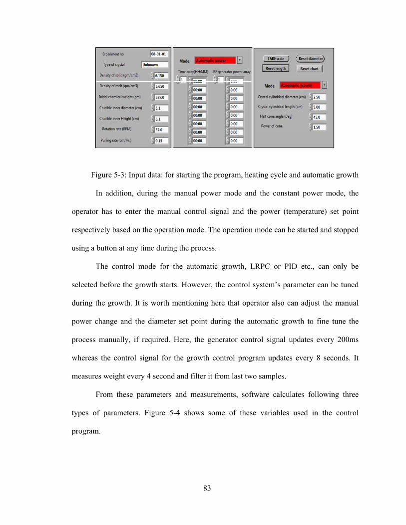
Figure 5-3: Input data: for starting the program, heating cycle and automatic growth
In addition, during the manual power mode and the constant power mode, the
operator has to enter the manual control signal and the power (temperature) set point
respectively based on the operation mode. The operation mode can be started and stopped
using a button at any time during the process.
The control mode for the automatic growth, LRPC or PID etc., can only be
selected before the growth starts. However, the control system’s parameter can be tuned
during the growth. It is worth mentioning here that operator also can adjust the manual
power change and the diameter set point during the automatic growth to fine tune the
process manually, if required. Here, the generator control signal updates every 200ms
whereas the control signal for the growth control program updates every 8 seconds. It
measures weight every 4 second and filter it from last two samples.
From these parameters and measurements, software calculates following three
types of parameters. Figure 5-4 shows some of these variables used in the control
program.
83

Figure 5-4: Various measurements, calculations and control parameters
General: crystal growth rate, crystal diameter, crystal calculated length, power
change (temperature), present output (i.e. control signal), remaining weight, remaining
time for heating or cooling cycle.
2
2
2
3
1
p conetotal cylindrical cone s cylindrical cylindrical
cylindrical cylindricaltotal cone cylindrical cone
p crucible
v tW W W r Lenth
Length rTime t t t
v R
π ρ⋅⎛ ⎞
= + = ⋅ ⋅ ⋅ +⎜ ⎟⎝ ⎠
⎛ ⎞= + = + ⋅ −⎜ ⎟⎜ ⎟
⎝ ⎠
(5-1)
• Set point or trajectory program: diameter set point, temperature set point.
• Growth parameters: time remaining during cone growth, calculated growth rate for
cylindrical part, present time for cone growth, total growth time, total weight and
84

percentage weight used. Approximate total growth time and total weight are
calculated before starting the growth, to help the operator, using the equation (5-1).
5.1.6 Development of the graphical user interface and LabVIEW software
LabVIEW software is preferred in order to develop the control program.
LabVIEW software using virtual instruments (VI) is more user friendly than the present
MicRicon controller is. It also has some advantage over other programming language like
C++. LabVIEW provides customizable controls and indicators in various formats e.g.
buttons, charts, values and characters that could easily adopted with the control software.
It has a benefit of running independent sequences or VI based on the requirement of the
program. The development of the LabVIEW program for the crystal growth control was
divided in various parts, or independent VI files, based on the objective. There are mainly
five independent VIs in this project.
• Global variables and graphical user interface (GUI): GUI is a center of the program
that enables the operator to use the control program effectively. GUI also allows the
operator to change the operation mode, control mode and process parameters. It
calculates set points for both the control programs, depending on the operation mode
of the process. It connects and calls all other VIs and uses global variable VI to share
various controls and indicators between them. Figure 5-5 shows GUI interface of the
program before starting the program.
85

Figure 5-5: Graphical user interface of LabVIEW control program
• Input and output: This VI measures required variables, power and weight, and
calculates growth rate, crystal diameter and crystal length. For simulation purposes,
the process model VI is developed in place of this program.
• Generator control VI: This program calculates the generator control signal based on
the error between a set point and the actual values, depending on the control mode
selected by the operator. The program also adds up positive feedback, calculated form
the growth control program, and present set point to calculate the new set point for
the generator control as shown in Figure 5-6. High limit and low limit of the power
adjustment are the constraints on the power control for crystal growth. They prevent
the crucible and the growth system from overheating, if the control program does not
86

work normally. As shown in the figure, diameter multiplier variable works like a flag
for auto (=1) and manual (=0) control program.
Figure 5-6: Generator set point calculation from the growth control feedback
• Growth control VI: This program calculates the control signal (or change of power)
required to change the diameter of the crystal. APPENDIX-B shows the algorithm
developed to calculate the control signal based on LRPC – MPC method discussed in
Chapter 3.3 .
• Data recording VI: This program records all the data in a text file in a suitable format.
This data can be used for later analysis.
5.1.7 Method of operation for the operator
This section describes the operation steps for the operator to grow a crystal, using
the developed control program. They are divided into four tasks.
• Start the process: Open GUI program and press the run button in LabVIEW to start
the program. The operator enters all initial growth parameters, as described above, on
the right side of the screen and then presses the start program button. Initially, the
87
program starts in the manual mode and will remain there for 30 seconds to reset all
the parameters, call all VIs and start measurements. At this time, the manual control
signal can be used to start the generator.
• Once the "STOP Operation Mode" button enables, the operator then can transfer from
manual mode to constant power mode. This process takes some time because the
control program runs until the control signal reaches the manual power set point for a
smooth transfer. In addition, any operation mode can be applied from the drop down
control and pressing “START Operation Mode” button respectively.
• Heating or cooling process: Once in automatic power mode, the operator enters the
temperature and time profile in the form of array and then presses the start button to
run the profile. When the process ends, it goes back to the constant power mode. The
operator can also stop the process at any time and the process will go back to the
constant power mode.
• Growth process: To start the growth process, the first job is the seeding process. The
operator can adjust temperature in the constant power mode. Once the seeding is
successful and stable, the process is ready for the automatic crystal growth. The
operator goes to automatic growth mode and enters the parameters that are needed for
the cone and cylindrical growth as discussed earlier. The control mode, LRPC or PID,
and initial gain parameters can also be selected before starting automatic growth. To
facilitate the proper parameter selection, the operator can see various calculated
growth parameters during these, as shown in Figure 5-4. The automatic growth
control can be started, after this. The process starts from the cone growth and ends
when the required crystal growth length of the cylindrical part is reached. During the
88

process, the operator can fine-tune the control system by changing the control
parameters. Even during the automatic mode, the operator can adjust manual power
change and diameter change without stopping the automatic control. At the end, the
crystal is pulled and the automatic growth mode is stopped. The crystal is then cooled
by using the automatic power mode and selecting the proper cooling profile.
However, the program can be interrupted at any time during the growth and the
process can be controlled from any other mode. This flexibility is good for any
immediate action, if needed, during the growth.
5.2 Initial parameters for new controller
In this section, some common problems that can affect crystal growth are
discussed. Later, the trajectory mapping and unit-less transformation of the control model
is presented. In addition, during the initial growth new controller had some problem to
control and model identification. After analyzing the data, the solution of this problem is
proposed here.
5.2.1 Common problems during crystal growth
The crystal growth process is inherently unstable. In fact, some time a very stable
crystal growth response can be an indication of a polycrystalline crystal rather than a
single crystal. The crystal growth process is a time consuming process that makes it more
vulnerable to the numerous instabilities that are uncontrollable. A slight change in any of
the process parameters can create an unstable growth. In my experience in the crystal
growth lab at University of Central Florida, I have faced many of these instabilities but
some of them have more profound effect on the control system than the others. Here,
89
some of these uncontrollable uncertainties are presented to explain the effect not only on
the crystal but also on the whole process.
• Power instability and the crystal growth loss: If the power fails during the crystal
growth process, the molten chemical solidifies at the surface. This causes the grown
crystal to be stuck with the solidified chemical in the crucible. However, due to the
rotation mechanism, the grown crystal keeps rotating. In this condition, the crystal
can brake from the seed. The seed holder can also be damaged. Figure 5-7 shows the
crucible with the solidified crystal and the seed holder because of the power failure
during the actual growth. Here, the crystal was broken from the seed holder. In
another case, instead of power failure, if the power dip is observed for just few
seconds then the diameter of the crystal can become unstable, which later on needs to
be controlled by the controller minimizing any abrupt power correction. In addition,
the power supply parameter like voltage and frequency keeps changing during the
entire growth and has profound effect on the crystal quality and growth stability.
• Cooling water instability: in crystal growth laboratory, the UCF physical plant
supplies chilled water. This water is used to cool the cooling water system by a heat
exchanger. The temperature change of this cooling water has a very significant effect
on the crystal growth. Especially, during the seeding when the temperature needs to
be adjusted very carefully and maintained precisely for long time. Any changes in the
chilled water temperature changes the temperature of the melt and creates instability
in the growth as discussed below.
90
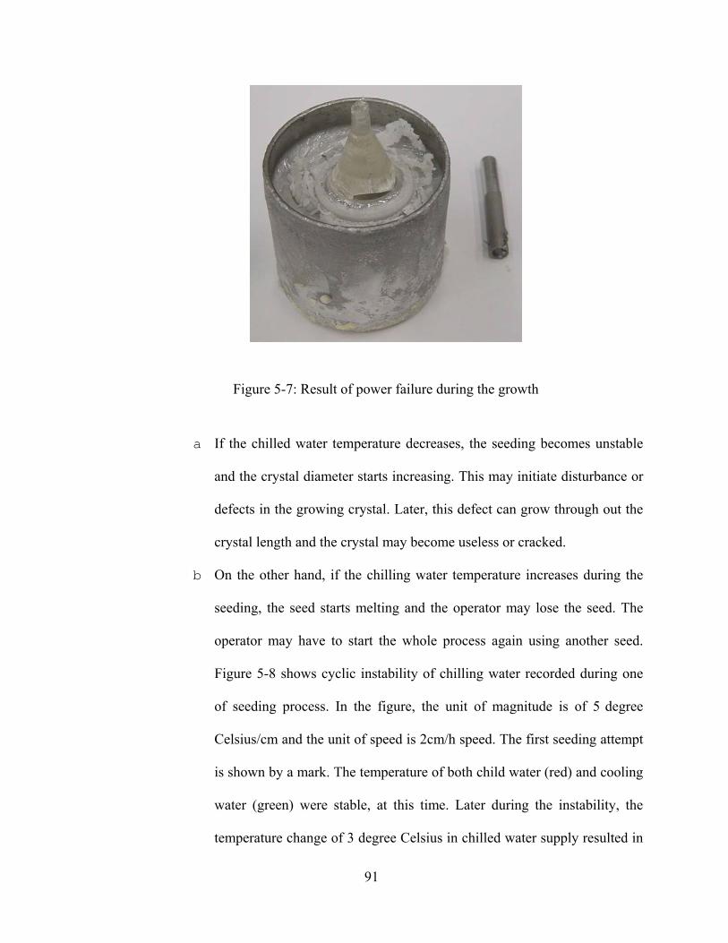
Figure 5-7: Result of power failure during the growth
a If the chilled water temperature decreases, the seeding becomes unstable
and the crystal diameter starts increasing. This may initiate disturbance or
defects in the growing crystal. Later, this defect can grow through out the
crystal length and the crystal may become useless or cracked.
b On the other hand, if the chilling water temperature increases during the
seeding, the seed starts melting and the operator may lose the seed. The
operator may have to start the whole process again using another seed.
Figure 5-8 shows cyclic instability of chilling water recorded during one
of seeding process. In the figure, the unit of magnitude is of 5 degree
Celsius/cm and the unit of speed is 2cm/h speed. The first seeding attempt
is shown by a mark. The temperature of both child water (red) and cooling
water (green) were stable, at this time. Later during the instability, the
temperature change of 3 degree Celsius in chilled water supply resulted in
91

about 6 degree Celsius temperature change in cooling water supply to the
growth chamber and heating coil. Multiple seeding attempts failed due to
the large temperature fluctuations. In the end, the seed was lost due to
melting. A new seed was installed and temperature was again adjusted for
seeding. The successful seeding took about 12 h.
Figure 5-8: Cooling water and chilled water temperature fluctuations
• Weighing error and effect on the controller: The weighing mechanism used for the
growth process has the tolerance of +/- 0.1 g. During the initial phase of the growth,
this could create problem in calculating growth rate. Figure 5-9 shows the growth rate
(g/h) calculated during the ideal or no growth condition for about 3 h. The calculate
diameter error from this weight noise could match the approximate diameter or the
growth rate required during the seeding (about 4 to 5 mm). The operator needs to
keep watching the seed growth until it stabilizes at a later part of the cone growth.
92

Hence, the automatic growth can only be started effectively once the diameter reaches
about 10 mm and growth is stabilized.
Figure 5-9: Diameter error due to weighing system noise
5.2.2 Input-output and set point calculations for control
Before presenting the result of the new control system, it is important to present a
few design parameters like the future prediction, order of the model and delay. The detail
description of different options and selections are presented here.
As discussed in earlier, the input-output model of the growth process was presented as a
unit-less model. Here, the feedback is positive as the process is already inverted. This
strategy helped to design the positive model of the process for control design. The input
of the model is the power change or unit-less actualP∆ . Equation (5-2) was applied to
ormalize the input. Here, the operator can define maximum and minimum from the
power required during seeding,
P∆
seedingP , by using variable . The power required during x
93
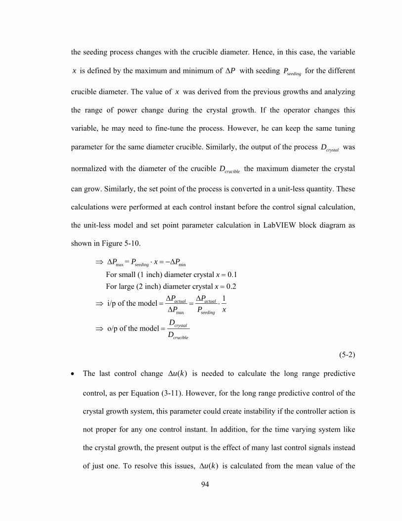
the seeding process changes with the crucible diameter. Hence, in this case, the variable
is defined by the maximum and minimum ofx P∆ with seeding seedingP for the different
crucible diameter. The value of was derived from the previous growths and analyzing
the range of power change during the crystal growth. If the operator changes this
variable, he may need to fine-tune the process. However, he can keep the same tuning
parameter for the same diameter crucible. Similarly, the output of the process was
normalized with the diameter of the crucible the maximum diameter the crystal
can grow. Similarly, the set point of the process is converted in a unit-less quantity. These
calculations were performed at each control instant before the control signal calculation,
the unit-less model and set point parameter calculation in LabVIEW block diagram as
shown in Figure 5-10.
x
crystalD
crucibleD
max min
max
=
For small (1 inch) diameter crystal 0.1 For large (2 inch) diameter crystal 0.2
1 i/p of the model
o/p of the model
seeding
actual actual
seeding
crystal
c
P P x P
xx
P PP P x
DD
⇒ ∆ ⋅ = −∆
==
∆ ∆⇒ = =
∆
⇒ =
⋅
rucible
(5-2)
• The last control change ( )u k∆ is needed to calculate the long range predictive
control, as per Equation (3-11). However, for the long range predictive control of the
crystal growth system, this parameter could create instability if the controller action is
not proper for any one control instant. In addition, for the time varying system like
the crystal growth, the present output is the effect of many last control signals instead
of just one. To resolve this issues, ( )u k∆ is calculated from the mean value of the
94
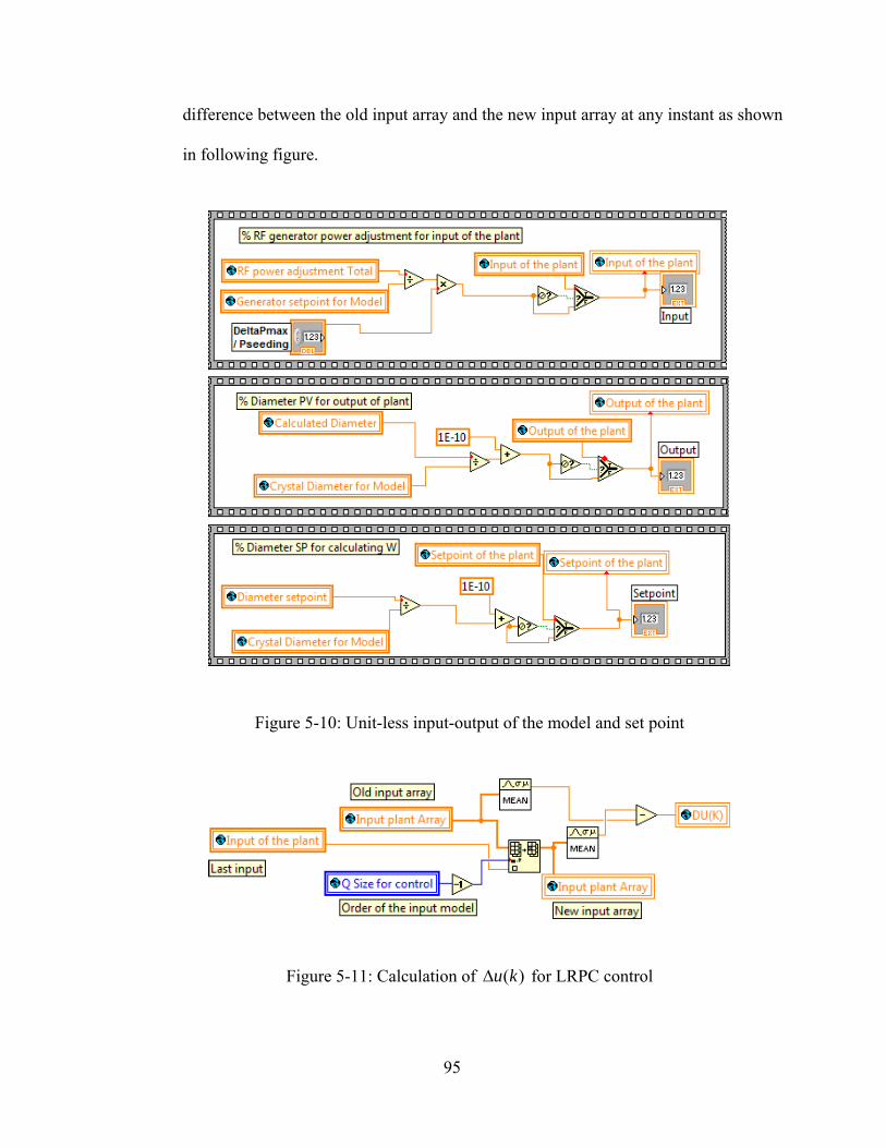
difference between the old input array and the new input array at any instant as shown
in following figure.
Figure 5-10: Unit-less input-output of the model and set point
( )u k∆Figure 5-11: Calculation of for LRPC control
95
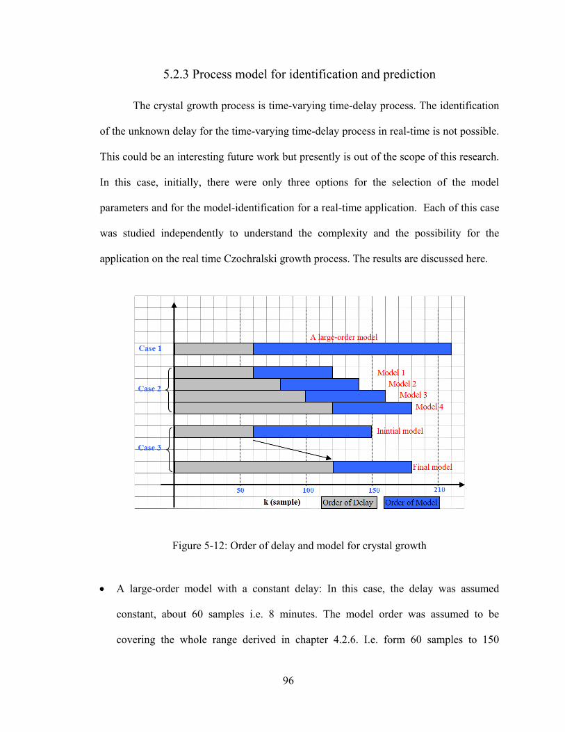
5.2.3 Process model for identification and prediction
The crystal growth process is time-varying time-delay process. The identification
of the unknown delay for the time-varying time-delay process in real-time is not possible.
This could be an interesting future work but presently is out of the scope of this research.
In this case, initially, there were only three options for the selection of the model
parameters and for the model-identification for a real-time application. Each of this case
was studied independently to understand the complexity and the possibility for the
application on the real time Czochralski growth process. The results are discussed here.
Figure 5-12: Order of delay and model for crystal growth
• A large-order model with a constant delay: In this case, the delay was assumed
constant, about 60 samples i.e. 8 minutes. The model order was assumed to be
covering the whole range derived in chapter 4.2.6. I.e. form 60 samples to 150
96

samples (from 10 to 20 minutes) as shown in the Figure 5-12. In this case, both the
identification process and LRPC program needs to solve the matrix inversion and the
recursive calculation to calculate the prediction and control signal. During the
development of the control program, it was observed that once the order of the model
is higher than 60 samples, the computational time for the complete control sequence
(i.e. identification + LRPC program) increases rapidly. Table 5-1 shows the average
computational time for each option measured on the actual control computer. In
addition, as the order of the model increases, the total calculation error increases. This
could affect the stability of the control system. Hence, this option was not a preferred
choice for the real-time control system of the crystal growth process. In the future,
when the computational power of computer and accuracy increases, this option could
be a better and simpler choice than the other choice described here.
Table 5-1: Computation time for different model
Option Order of Delay Order of model Computational time
1 60 80 5 second
60 100 6.5 second
60 120 8.5 second
60 150 11 second
2 60 , 80, 100, 120 60 6 second3 60 60 4 second
• Multiple models with the same order but different delay: In this case, four models
were considered with the same order (i.e. 60 samples = 8 minutes) for the whole
control range. The order of the delay for each one was considered different (i.e. from
97

60, 80, 100, 120 samples). Thus, the predictive horizon can be covered completely.
Here, the lower order models are preferred to reduce computational time to less than
8 sec for real-time application. The gain scheduling for each model was carried out
based on the relation between the delay and the length of the crystal described in
chapter 4.2 . The length of the crystal was divided into three parts from initial length
to final length. Figure 5-13 is a graphical representation of the gain scheduling for
each model as the growth progresses. This kind of gain scheduling gives a smooth
transfer to the delay-based control from one model to another. The problems related
to this case are discussed here.
a In this case, the identification and LRPC program have too many variables
(about 4 times than normal). The total no of calculations for control
increases (four times than the earlier case at each stage of LRPC program).
It increases complexity during designing and rectifying errors of the
control program.
b In addition, the software shares some of the same standard subroutine Vis.
This sharing could lead to confusion and control signal error.
c The operator needs to change all of the models parameters with different
types of crystal growths. This could be a complicated task. Any wrong
parameter selection can create a problem during real-time growth.
d If any of the identification process or the LRPC calculation becomes
unstable at any stage of the growth, the error or the wrong control signal
( ) propagates to all models and their control programs. ( )u k∆
98

e Crystal 4 and Crystal 5 were grown using this technique. Few simulations
were also run based on this case, but they were either found to be too
complex or too cumbersome for real-time operation. In the future, if one
can check stability of both the program and model by some means during
real-time growth then this case could become a possibility.
Gain 1
Gain 2
Gain 3
Gain 4
Part 1 Part 2 Part 3
LI LT
Figure 5-13: Gain scheduling for multiple model LRPC technique
• One model with the time varying predictive horizon based on the delay: The last
option was to consider only one model and reduce the complexity. This model can be
configured with the time varying delay. In other words, the control horizon is
changing as the time delay changes with the crystal length. The control program uses
a prediction based on this model to compare with the calculated trajectory. Here, the
order of the model is 60 samples (8 minutes). The delay range changes as the growth
99

progress (function of crystal length) from 60 to 120 samples (about 8 to 20 minutes)
as presented in chapter 4.2 and Figure 5-12. The model will adopt slowly with the
identification process as the growth progress and delay changes. In this case, the
complexity of the calculation decreases substantially. With this delay mapping, this
option of one model with time-varying predictive horizon seems more suitable at
present. Crystal 6 to Crystal 12 were grown from this method. The other two options
need further improvement in the hardware and the program that are beyond the scope
of the study at this time.
5.2.4 Data accumulation for model identification
Once the model parameter for the model identification is defined, the next step is
to establish the stable model identification method. For any model identification process,
some initial input-output data are required to initialize the model. For real-time model
identification, these data are gathered online. The time it takes to gather this data
depends upon the validation of the data, the order of input-output model and the time
delay. Once the suitable data are available, the model identification process starts.
Initially, the recursive model identification is not accurate. It takes a lot of iteration
before the derived model is stabilized. The model is then useful for further control system
calculations. All this time for gathering data and initializing iterations, the process has to
be running in automatic control mode. In addition, for the crystal growth process, the
input-output data seems meaningful for identification once the diameter reaches about 1
cm. For less than 1 cm diameter, the control signal and its effect on the growths is almost
negligible due to weighing mechanism error. Hence, data gathered during the diameter
less than 1 cm is not reliable for modeling. During this time the MRAC technique,
100
discussed in chapter 4.1.2, was applied for controlling the process. In other words, when
the operator starts the automatic control mode, the process is controlled by MRAC
technique. Once the diameter reaches 1 cm, the model identification process starts
gathering the initial data and prepares the input and output arrays. The total number of the
samples for data gathering and initial model identification was selected as 300 (about two
times of the order of the model plus delay), which is equals to 40 minutes with 8 second
per sample rate.
max
max max
1. 60 Order of the model2. Starting point: = 5 300; Ending point: 15 9003. if 300 LRPC gain 0; MRAC gai
actual
flagflag flag
flag
= =
⋅ = = ⋅ =<
⇒ = n = 1- LRPC gain
max
max
4. if 300 900 5 LRPC gain = ; MRAC gain = 1- LRPC gain
(15 5)3. if 900 LRPC gain 1; MRAC gain =
actual
actual
actual
flagflag flag
flagflag
≤ <− ⋅
⇒− ⋅
≤⇒ = 1- LRPC gain
(5-3)
Once the data are available and LRPC program is ready to control the process, the
software needs to transfer the control from the MRAC to LRPC smoothly. This transfer
cannot be achieved in one-step. The control is transferred from the MRAC to LRPC
program slowly and linearly (from 0% to 100%) as crystal grows. To achieve this goal,
the gains of MRAC and LRPC were developed by applying gain scheduling. The control
program takes another 600 samples (about 80 minutes) to transfer control from MRAC to
LRPC technique. The time (in form of no of samples) it takes to change control from the
MRAC to LRPC could be adjusted, if required, based on the type of crystal, pulling speed
101

and growth rate instead of 600 samples. At present, a variable named flag was created
to track the sample number and calculates gains as shown in Equation (5-3).
5.2.5 Calculating set point trajectory
For the LRPC technique, the set point trajectory is required to calculate the total
error for the control program. The starting point for this trajectory mapping is the order of
time delay for the crystal growth process. The initial point ( 1w k )+ of the trajectory was
considered to be the present output (percentage crystal diameter) of the process. The
length (or order) of the trajectory is the length of the control horizon considered for
LRPC design. The modeling data for the trajectory is presented in Equation (5-4).
1 min
2
Starting horizon 1Ending horizonOrder of trajectory = 1u a
N dN d N
N N n
= = += = +
= = +
(5-4)
The process set point was calculated from the growth data, selected by the
operator. Here, the maximum rate of diameter change for the trajectory was defined by
the half cone angle as shown in Equation (5-5) to calculate the ending point,
. This rate is a constrained on the trajectory mapping and can be adjusted
by the operator. The exponential factor
max( aw k d N+ + )
α was adjusted to 0.98.
Figure 5-14 shows two graphs. One graph shows the trajectory ( ) from the
present output (0.482) to the set point (0.499). Here, 160 samples is the order (length) of
the trajectory. The other graph with two pointers shows both a prediction (purple line,
calculated from the model) and a trajectory (yellow line, calculated from the set point)
used for the control signal calculation for 15 minutes. One can see that at one point the
1wNW ×
102
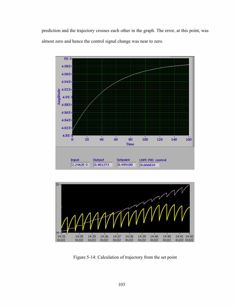
prediction and the trajectory crosses each other in the graph. The error, at this point, was
almost zero and hence the control signal change was near to zero.
Figure 5-14: Calculation of trajectory from the set point
103
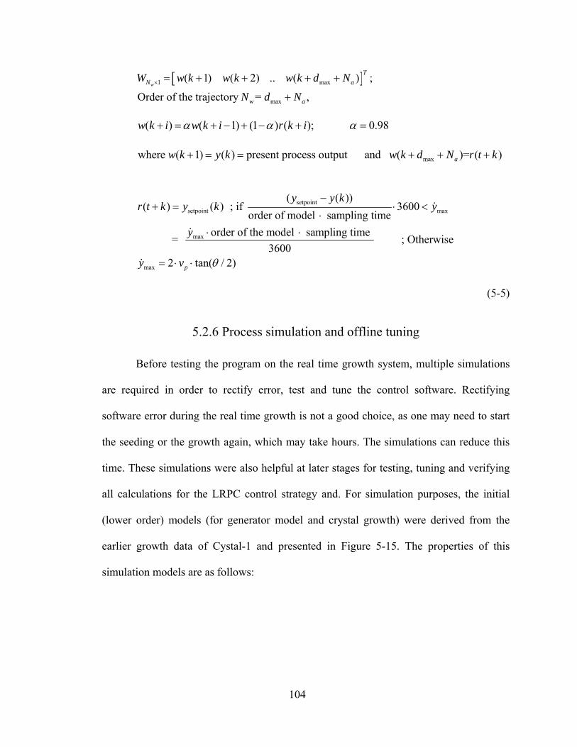
[ ]1 m
max
( 1) ( 2) .. ( )
Order of the trajectory = ,w
TN a
w a
W w k w k w k d N
N d N× = + + + +
+ax ;
( ) ( 1) (1 ) ( ); 0.98 w k i w k i r k iα α α+ = + − + − + =
maxwhere ( 1) ( ) present process output and ( )= ( ) aw k y k w k d N r t k+ = = + + +
setpointsetpoint max
max
max
( ( ))( ) ( ) ; if 3600
order of model sampling timeorder of the model sampling time = ; Otherwise
36002 tan( / 2)p
y y kr t k y k y
y
y v θ
−+ = ⋅ <
⋅⋅ ⋅
= ⋅ ⋅
&
&
&
(5-5)
5.2.6 Process simulation and offline tuning
Before testing the program on the real time growth system, multiple simulations
are required in order to rectify error, test and tune the control software. Rectifying
software error during the real time growth is not a good choice, as one may need to start
the seeding or the growth again, which may take hours. The simulations can reduce this
time. These simulations were also helpful at later stages for testing, tuning and verifying
all calculations for the LRPC control strategy and. For simulation purposes, the initial
(lower order) models (for generator model and crystal growth) were derived from the
earlier growth data of Cystal-1 and presented in Figure 5-15. The properties of this
simulation models are as follows:
104

Figure 5-15: Block diagram of the crystal growth model for simulation
• The output of the generator model is considered as an input of the growth model. The
growth model calculates the new weight change of simulated growth.
• This weight change is integrated with the old weight to calculate present crystal
weight. This weight is passed through the normal measurement cycle for filtering and
calculating the growth rate and diameter.
• Based on this calculated diameter and the set point diameter, the control program
calculates the control signal P∆ . Using this P∆ and present set point, the generator
control program calculates the control signal for the generator. This control signal
becomes the input of the generator model. This completes the simulation.
105

• Some non-linearities were added to the growth model based on the experimental
results discussed earlier to check the robustness of the program. First, adjustable
white noise function with standard deviation and mean is added to weighing signal. In
addition, the effect of power change as the melt level goes down is added in form a
linear function.
5.3 Instability and model identification
After selecting the control mode and the model parameters for the identification
and predication, the control program was initially tested and tuned with the simulation.
The initial gain parameters for the LRPC MPC programs were tuned. These results were
later tested to grow Crystal-4 and Crystal-5, as shown in Figure 5-16 and Figure 5-17
respectively, with online model identification. However, the growth system was not
stable after a while. The structure of the growth system inside the furnace along with the
crucible and other parameters were kept similar to the earlier growth described in Chapter
4.1.1. The set point diameter for the cylindrical portion was 33 mm. The diameter of the
crucible was 55 mm and the rotation rate was kept at an optimal level of 32 rpm for the
flat interface. The half cone angle for both crystals was kept constant also. The growth
parameters for these crystals are shown in Table 5-2 and Table 5-3.
106

CGEL
Crystal Growth & Epitaxy LaboratoryAMPAC/UCF
Figure 5-16: Crystal-4 grown with model identification
Table 5-2: Growth parameter for Crystal-4
Material LGT Growth rate for cylindrical part 19.33 g/hCrucible internal diameter 5.1 mm Total cone growth time 9.2 hInitial weight 515 g Total growth time 22.6 hInitial melt level 41.2 mm Total weight 295 gCrystal diameter 33 mm % Chemical used 57%Pulling speed 2 mm/ h Total calculated length of crystal 54 mmRotation speed 32 rpm
Half cone angle 45o Crystal final weight 149.55 gPower of cone 1.2 Actual Crystal length 60 mmCylindrical crystal length 50 mm Actual growth time 23 h
P I 1/For MRAC 1 0.3 1000LRPC-MPC Initial gain --- --- ---LRPC-MPC After tuning --- --- --
Controller gains
Calculated parameter before growthInitial parameter
After growth parameter
Gain
Growth parameters for Crystal- 4
107
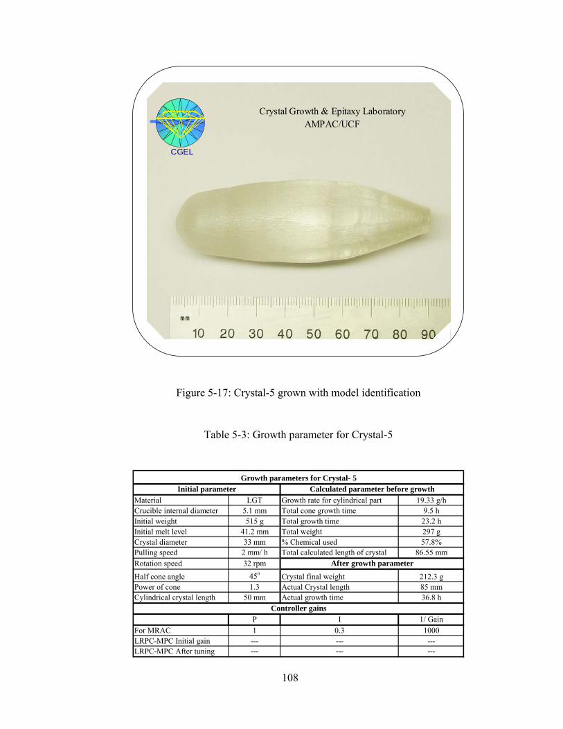
CGEL
Crystal Growth & Epitaxy LaboratoryAMPAC/UCF
Figure 5-17: Crystal-5 grown with model identification
Table 5-3: Growth parameter for Crystal-5
Material LGT Growth rate for cylindrical part 19.33 g/hCrucible internal diameter 5.1 mm Total cone growth time 9.5 hInitial weight 515 g Total growth time 23.2 hInitial melt level 41.2 mm Total weight 297 gCrystal diameter 33 mm % Chemical used 57.8%Pulling speed 2 mm/ h Total calculated length of crystal 86.55 mmRotation speed 32 rpm
Half cone angle 45o Crystal final weight 212.3 gPower of cone 1.3 Actual Crystal length 85 mmCylindrical crystal length 50 mm Actual growth time 36.8 h
P I 1/ GainFor MRAC 1 0.3 1000LRPC-MPC Initial gain --- --- ---LRPC-MPC After tuning --- --- ---
Controller gains
Calculated parameter before growthInitial parameterGrowth parameters for Crystal- 5
After growth parameter
108

5.3.1 Results and analysis for Crystal-4 and Crystal-5
Crystal 4 was grown with the multiple model identification with multiple delay
(case 2) as discussed in chapter 5.2.3. This was the first crystal that was grown using the
long range predictive control method. Initially, the model reference adaptive controller
controlled the crystal growth. Once the model was identified for prediction, the control
was transferred to long range predictive controller, as discussed in chapter 5.2.4. As
shown in Figure 5-18 , during the cone growth part, the growth was stable. During this
time, the control strategy was being transferred from the MRAC to LRPC technique. The
control program was able to transfer smoothly from the MRAC to LRPC before the cone
growth reached about 60% of the final diameter.
Growth of Crystal-4
0
1
2
3
4
0 200 400 600 800 1000 1200 1400
Time (minute)
% P
ower
cha
nge
0
20
40
60
80
% D
iam
eter
% Pow er change % Diameter % Diameter SP
Figure 5-18: Diameter and power change graph for Crystal-4
109
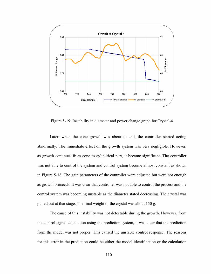
Growth of Crystal-4
2.65
2.75
2.85
2.95
700 720 740 760 780 800 820 840 860
Time (minute)
% P
ower
cha
nge
63
66
69
72
% D
iam
eter
% Pow er change % Diameter % Diameter SP
Figure 5-19: Instability in diameter and power change graph for Crystal-4
Later, when the cone growth was about to end, the controller started acting
abnormally. The immediate effect on the growth system was very negligible. However,
as growth continues from cone to cylindrical part, it became significant. The controller
was not able to control the system and control system become almost constant as shown
in Figure 5-18. The gain parameters of the controller were adjusted but were not enough
as growth proceeds. It was clear that controller was not able to control the process and the
control system was becoming unstable as the diameter stated decreasing. The crystal was
pulled out at that stage. The final weight of the crystal was about 150 g.
The cause of this instability was not detectable during the growth. However, from
the control signal calculation using the prediction system, it was clear that the prediction
from the model was not proper. This caused the unstable control response. The reasons
for this error in the prediction could be either the model identification or the calculation
110

of the control system. Using a known stable model, the simulation was run to test the
calculation. The control signal calculations were normal and the control was able to
transfer smoothly from the MRAC to LRPC technique. Hence, the model identification
process was the main problem for the instability.
During the growth, it was not possible to study the identified model for stability.
Later, the growth data gathered during the growth process was analyzed. Offline model
identification was run to check the prediction and the model stability. To test the stability
of the model during the model identification, a step response method was designed which
can be introduced at any time during the identification. It gives the step response of the
present identified model whenever interrupted during the process. The stability of the
model was tested for the entire length of the grown crystal. From this analysis, the
identified model was found stable initially, during the initial part of the cone growth.
Near the end of the cone growth and beginning of the cylindrical growth, there were
some unexpected peaks (variations) in the diameter measurement as shown in Figure
5-19. For the long-range model identification, it could cause unstable model
identification.
Once the model becomes unstable, the prediction error propagates not only to the
control system but also to the next identification process. The identification process was
not able to derive a stable model again even though the growth was stable later. This led
to control structure failure. In control system terminology, this is explained by a
bifurcation theory when the process becomes unstable to stable or vice verse. Many
researchers have studied the control system design for such systems. However, the model
identification of the unstable process with bifurcation is yet to be explored.
111

Growth of Crystal-5
-0.5
0
0.5
1
1.5
170 470 770 1070 1370 1670 1970
Time (minute)
% P
ower
cha
nge
-25
0
25
50
75
% D
iam
eter
% Pow er change % Diameter % Diameter SP
Manual power adjustment
Figure 5-20: Diameter and power change graph for Crystal-5
Growth of Crystal-5
0.18
0.21
0.24
0.27
0.3
700 750 800 850 900 950
Time (minute)
% P
ower
cha
nge
53
56
59
62
65
% D
iam
eter
% Pow er change % Diameter % Diameter SP
Manual power adjustment
Figure 5-21: Instability in diameter and power change graph for Crystal-5
112

To test this hypothesis, Crystal-5 was grown with the similar growth parameters
as shown in Figure 5-17. The power of cone was changed to 1.3 as shown in Table 5-3 to
increase the cone growth time and achieve a stable transfer from the cone to cylindrical
part. However, similar results were achieved during the growth as shown in Figure 5-20.
The control was unstable near the same area as shown in the Figure 5-21. The data was
gathered and analyzed for stability as discussed above. It was clear that this identification
method was not able to derived stable model in case any instability in the process. For
this reason, a study of partial model identification and design control system could be a
better option e.g. by filtering the diameter for unstable frequency or partially defined (or
bounded) model parameter. However, it is the beyond the scope of this study. The idea of
real time model identification process with ability to check model stability parameter is
left for future work.
5.3.2 Predefined model for long range predictive control
The main objective of this study was to incorporate the delay in the control
system and predictive horizon. The time delay variation during the growth is more
important factor than the model itself. For prediction, one can apply a predefined model
that is derived from the old growth. In fact, multiple models, derived from different
crystal region, could be an option but not preferable. At this point only one stable growth
model, derived from comparing previous growth data with the stable model of the filter,
was used to define the control process. (i.e. indirect control instead of direct control).
The step response parameters for the actual growth like rise-time and settling time were
compared with derived model for stability. Figure 5-22 and Figure 5-23 shows the step
response of the derived model and parameter for the time response. Figure 5-24 and
113
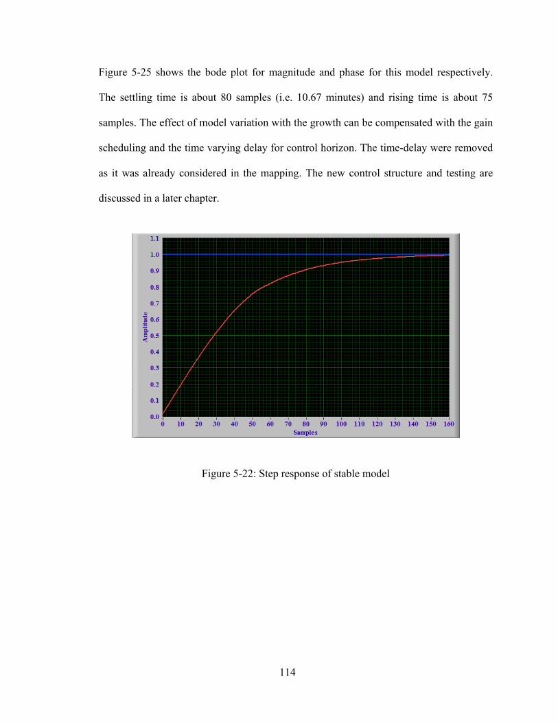
Figure 5-25 shows the bode plot for magnitude and phase for this model respectively.
The settling time is about 80 samples (i.e. 10.67 minutes) and rising time is about 75
samples. The effect of model variation with the growth can be compensated with the gain
scheduling and the time varying delay for control horizon. The time-delay were removed
as it was already considered in the mapping. The new control structure and testing are
discussed in a later chapter.
Figure 5-22: Step response of stable model
114

Figure 5-23: Time response parametric data for the model
Figure 5-24: Magnitude: bode plot for the derived model
115

Figure 5-25: Phase: bode plot for the derived model
116

CHAPTER 6: IMPLEMENTATION OF LRPC CONTROL
In the last chapter, the initial result for the LRPC control system with the online
model identification was discussed. The problem of the unstable model identification
during the growth, if there is any disturbance in the growth, made the proposed control
strategy unsuitable for the real time crystal growth. The other alternative was to apply a
pre-derived stable model of the crystal growth for the control system. In other words, an
indirect control strategy was adopted instead of an earlier proposed direct control
strategy.
In this chapter, this indirect control strategy with a new control model is
presented. Later, an another control strategy named LRPC PID, other than LRPC MPC
discussed in Chapter 3, was also considered for the study. The LRPC PID is similar to
LRPC MPC. However, it calculates a control signal using PID instead of MPC technique
from the error between the prediction (done by the model) and trajectory (calculated from
the set point).
6.1 Modified control model
The assumptions for the new control system remain the same as presented earlier
in section 5.1.2. Following are the main differences in a new controller structure.
• The third task has been changed. Instead of the model identification, a predefined
model is used to calculate the prediction based on the LRPC technique.
• Automatic changeover of the main control technique from the MRAC to LRPC is
discussed in the last chapter needs to be tested again. However, as the model is
already pre-derived, there is no need to use MRAC initially and later transfer to
117

LRPC slowly during the cone growth. If this transfer is not needed, it cab be removed
from the control structure.
• To compensate the effect of using only one model instead of the time-varying model
of crystal growth, the time varying delay mapping and gain mapping are considered
for prediction. These mappings were divided in ten parts depending on the length of
the crystal grown as shown in following Figure 6-1. These mapping were derived
from the earlier experimental results of crystal 1 to 3.
• The control parameters for the model and delay and the trajectory mapping are
similar discussed in chapter 5.3 . The control horizon for trajectory was 240 samples
(or control instants). Figure 6-1 also shows the other controller parameter like a and
along with the order of the denominator and numerator . These values were
tuned during simulation and real-time growth.
l aN bN
Figure 6-1: Gain and delay mapping and controller parameter
118

• Here, the delay increases as the melt level decreases or the crystal length increases.
As the crystal length changes, software considers new delay and gain based on above
mapping. The software uses this delay to compare the difference between the
trajectory and prediction.
• The gain mapping is to adjust the controller gain as the crystal growth progress and
the melt level goes down. Generally, the gain does not change much during the initial
part of the growth. However, when the melt level goes down, the controller needs to
adjust the power change faster than usual, even though the delay is increasing. The
gain was slowly decreasing during the initial part of cylindrical growth. At 50% of
the cylindrical length, the gain becomes constant. When the length reaches about
70%, the gain starts increases because of very low melt level. Fine-tuning for these
parameters was done during the actual growth.
At this point, the complete control structure was known. The simulation and
tuning were carried out before testing on the actual growth. Other process parameters for
the growth, like optimum rotation, pulling speed and cylindrical diameter, still need to be
adjusted in terms of stability. The effect of instabilities also needs to be tested during the
growth to check the stability of the control system. For that reason, a total six crystals
were grown (three for each control technique). The growth parameters, results and
observations are discussed for each crystal growth in the next sections. At the end, a
large-diameter crystal was grown to check the final control system.
119
6.2 Long range predictive PID control and crystal growth
Traditionally, the PID controllers have been in use for many processes. However,
the application to the time delayed process has not been studied extensively. Here, the
sake of comparison, a long range predictive PID control system is also considered for the
crystal growth process. The controller structure and other specification are similar to the
LRPC-MPC based controller.
6.2.1 Introduction of PID control
In this section, a long range predictive PID control (LRPC- PID) is presented. It is
similar to the long range model predictive control (MPC). The only difference is in the
control signal calculation for the prediction horizon. It calculates control signal using PID
technique, which consists of three basic terms, P (proportional), I (integral), and D
(derivative). However, instead of using the present error term only, this control considers
the error between the trajectory and the predicted output of the system for the prediction
horizon. That means each prediction point has an independent error and a controller with
it. The benefit of such control strategy is that it can incorporate the delay of the system
irrespective of the order of the system. The optimal tuning of PID gains can be achieved
during the actual growth or by comparing them with the MPC control technique. Detailed
description and explanation is discussed in [16]. In general, the control signal ( ( )u k∆ )
can be calculated from the following equation, which is analogues to the equation (3-11).
1
1
( ) ( ) ( ) ( ( ) ( 1)
ˆ( ) ( ( ) ( | ))
= Total error between predicted output and trajectory over the control horizon
k
p i di
k
i
u k k e k k e k k e k e k
e k w k i y k i k
=
=
= ⋅ + ⋅ + ⋅ − −
= + − +
∑
∑
120
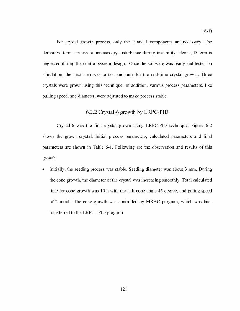
(6-1)
For crystal growth process, only the P and I components are necessary. The
derivative term can create unnecessary disturbance during instability. Hence, D term is
neglected during the control system design. Once the software was ready and tested on
simulation, the next step was to test and tune for the real-time crystal growth. Three
crystals were grown using this technique. In addition, various process parameters, like
pulling speed, and diameter, were adjusted to make process stable.
6.2.2 Crystal-6 growth by LRPC-PID
Crystal-6 was the first crystal grown using LRPC-PID technique. Figure 6-2
shows the grown crystal. Initial process parameters, calculated parameters and final
parameters are shown in Table 6-1. Following are the observation and results of this
growth.
• Initially, the seeding process was stable. Seeding diameter was about 3 mm. During
the cone growth, the diameter of the crystal was increasing smoothly. Total calculated
time for cone growth was 10 h with the half cone angle 45 degree, and puling speed
of 2 mm/h. The cone growth was controlled by MRAC program, which was later
transferred to the LRPC –PID program.
121
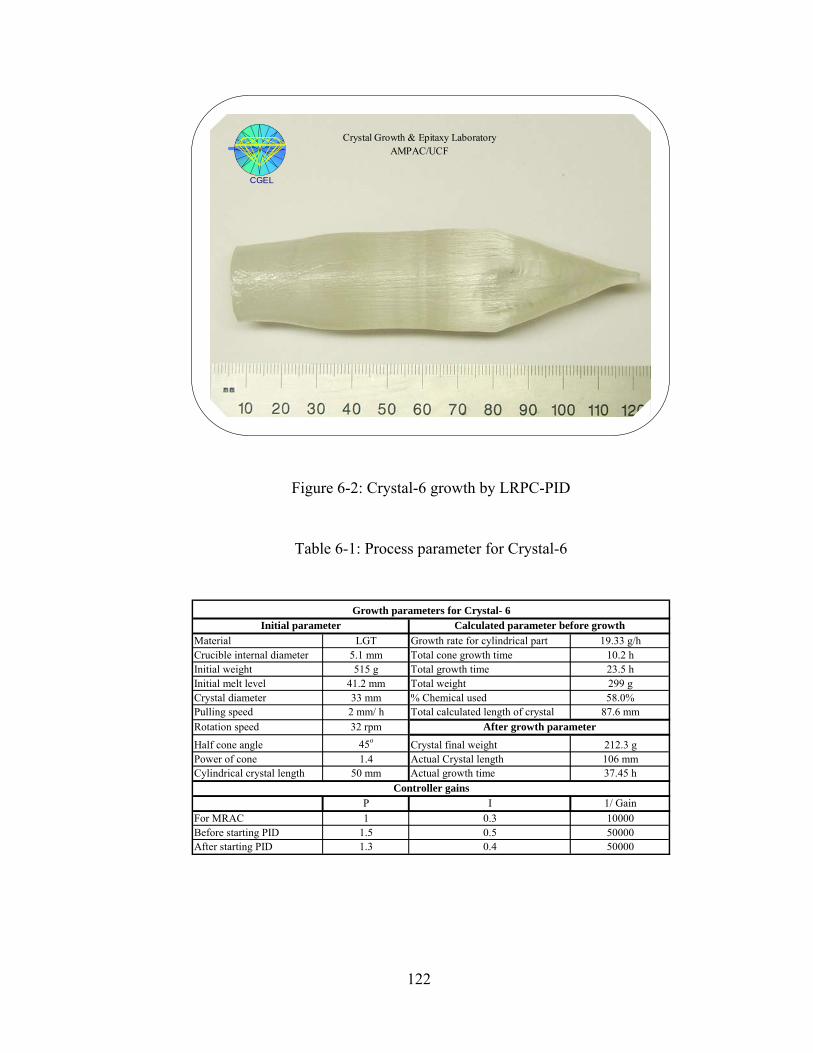
CGEL
Crystal Growth & Epitaxy LaboratoryAMPAC/UCF
Figure 6-2: Crystal-6 growth by LRPC-PID
Table 6-1: Process parameter for Crystal-6
Material LGT Growth rate for cylindrical part 19.33 g/hCrucible internal diameter 5.1 mm Total cone growth time 10.2 hInitial weight 515 g Total growth time 23.5 hInitial melt level 41.2 mm Total weight 299 gCrystal diameter 33 mm % Chemical used 58.0%Pulling speed 2 mm/ h Total calculated length of crystal 87.6 mmRotation speed 32 rpm
Half cone angle 45o Crystal final weight 212.3 gPower of cone 1.4 Actual Crystal length 106 mmCylindrical crystal length 50 mm Actual growth time 37.45 h
P I 1/For MRAC 1 0.3 10000Before starting PID 1.5 0.5 50000After starting PID 1.3 0.4 50000
Controller gains
Calculated parameter before growthInitial parameter
After growth parameter
Gain
Growth parameters for Crystal- 6
122

• The cone growth took around 15 h to reach the cylindrical diameter that is
approximately 30 degree cone angle. The cone growth was stable until the crystal
diameter reached to cylindrical diameter (33 mm). At the end of the cone growth,
there was some uncertainty and diameter increased rapidly. From the grown crystal,
near end of the cone growth, the crystal developed crack internally. It could be due to
the unstable flat interface. The diameter set point could have been slightly too high
for the present rotation rate (32 rpm).
• The crystal growth was stable after the cone growth. However, the crystal diameter
decreased at around 75% of the melt level (about 20 h). Some inclusions/voids were
visible inside the grown crystal.
• Once the growth interface and growth became unstable, the control software could
not stabilize the crystal diameter by adjusting the generator power. As shown in the
graph, percentage power change was about 3%. The normal power change should be
around 1%.
• At 50% of the melt level, the diameter decreased again and decreased continuously.
The growth was completely unstable even though the total power change was about
6%. This could be due to polycrystalline growth or the set point of the crystal
diameter was high, which resulted in unstable growth interface.
• After about 38 h, the crystal growth was aborted. It took about 14 h more time than
calculated.
123

Growth of Crystal-6
0
1.5
3
4.5
6
0 400 800 1200 1600 2000 2400
Time (minute)
% P
ower
cha
nge
0
20
40
60
80
% D
iam
eter
% Pow er change % Diameter % Diameter SP
Figure 6-3: Diameter and power change graph for Crystal-6
Growth of Crystal-6
44
58
72
86
100
0 400 800 1200 1600 2000 2400
Time (minute)
% M
elt l
evel
0
25
50
75
100
% C
ryst
al le
ngth
% Melt level % Crystal length
Figure 6-4: Crystal length and melt level graph for Crystal-6
124

6.2.3 Crystal-7 growth by LRPC-PID
Crystal-7 was again grown using LRPC-PID technique. Figure 6-5 shows the
grown crystal. From the results of the last growth, diameter set point for the crystal was
reduced to 28 mm from 32 mm. The power of the cone was also increased to make the
cone to cylinder transfer smoother. The total time of cone growth was reduced to 9 h This
reduced the total calculated weight also. Other growth parameters, calculated parameters
and final parameters are shown in Table 6-2. Following are the observation and results of
this growth.
CGEL
Crystal Growth & Epitaxy LaboratoryAMPAC/UCF
Figure 6-5: Crystal-7 growth by LRPC-PID
125

Table 6-2: Process parameter for Crystal-7
Material LGT Growth rate for cylindrical part 11.27 g/hCrucible internal diameter 5.1 mm Total cone growth time 9 hInitial weight 515 g Total growth time 25.5 hInitial melt level 41.2 mm Total weight 212.2 gCrystal diameter 28 mm % Chemical used 41.0%Pulling speed 2 mm/ h Total calculated length of crystal 62 mmRotation speed 32 rpm
Half cone angle 45o Crystal final weight 188.65 gPower of cone 1.5 Actual Crystal length 80 mmCylindrical crystal length 50 mm Actual growth time 27.1 h
P I 1/LRPC-MPC Initial gain 1 0.4 50000LRPC-MPC After tuning 1 0.35 50000
Controller gains
Calculated parameter before growthInitial parameter
After growth parameter
Gain
Growth parameters for Crystal- 7
• The growth model for the prediction was already derived before the growth. Hence,
LRPC –PID control system can be applied during initial growth without MRAC, if it
is pre-tuned. Here during the actual growth, MRAC program was controlling the
growth during the initial part of the growth. However, in this growth, instead of a
smooth transfer from the MRAC to LRPC-PID technique, an instant transfer (one-
step transfer) was opted during the growth (at time t= 175 minute). This instant
transfer caused a jump in control signal (power change) but had nominal effect on the
crystal diameter.
• After the seeding, the calculated seeding diameter was about 6 mm (20% of final
diameter). This indicates that the seeding was not proper as can be seen by Figure
6-5. However, the starting point of the set point for crystal diameter was kept at the
actual diameter. During the cone growth, crystal growth was stable and crystal grew
at a 30 degree half cone angle. It took about 10 h to reach at the cylindrical diameter.
126

• Near the end of the cone growth, the diameter overshoot was observed, similar to the
last growth. The controller adjusted the control signal. At one point, the control signal
became negative and remained negative for about 5 h In other words, the crystal was
growing at the same power as of seeding, which is unusual but indicates the controller
was working normally. The crystal diameter remained high for about 9 h. The defects
were clearly visible inside the crystal in this region. The growth interface was not
stable. To stabilize it, the crystal diameter of the rotation rate had to be adjusted.
• Again, in the actual crystal, a crack was developed during the end of the cone growth,
similar to the last growth. The reason could be due the diameter jump and seeding
problem or higher value of the crystal diameter for the rotation rate.
• Later at 75% of the melt level, the crystal diameter decreased and kept decreasing for
the remaining growth. Due to this instability, the crystal was pulled out earlier than
calculated. The final melt level was 60%; where as the weight of the crystal was
about 189 g.
• The gain tuning for PID controller was carried out online. It was clear from the error
and control signal calculations that the controller was working properly.
127

Growth of Crystal-7
-0.5
0
0.5
1
1.5
2
0 400 800 1200 1600
Time (minute)
% P
ower
cha
nge
0
15
30
45
60
75
% D
iam
eter
% Pow er change % Diameter % Diameter SP
Figure 6-6: Diameter and power change graph for Crystal-7
Growth of Crystal-7
60
70
80
90
100
0 400 800 1200 1600
Time (minute)
% M
elt l
evel
0
25
50
75
100
% C
ryst
al le
ngth
% Melt level % Crystal length
Figure 6-7: Crystal length and melt level graph for Crystal-7
128

6.2.4 Crystal-8 growth by LRPC-PID
During the last crystal growth, the crystal diameter was adjusted to reduce
instability and eliminate cracks but still there were instability and cracks. This time,
instead of crystal diameter, the rotation rate was decreased to 25 rpm from 32 rpm. This
could help to stabilize the interface shape by making it convex instead of flat. Crystal-8
was grown using LRPC-PID technique. Figure 6-8 shows the grown crystal. Other
growth parameters, calculated parameters and final parameters are shown in Table 6-3.
• For this growth, only LRPC-PID control was considered. The MRAC control is not
needed when the model identification process was not applied for real time growth.
CGEL
Crystal Growth & Epitaxy LaboratoryAMPAC/UCF
Figure 6-8: Crystal-8 growth by LRPC-PID
129
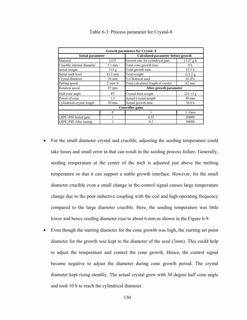
Table 6-3: Process parameter for Crystal-8
Material LGT Growth rate for cylindrical part 11.27 g/hCrucible internal diameter 5.1 mm Total cone growth time 9 hInitial weight 515 g Total growth time 25.5 hInitial melt level 41.2 mm Total weight 212.2 gCrystal diameter 28 mm % Chemical used 41.0%Pulling speed 2 mm/ h Total calculated length of crystal 62 mmRotation speed 25 rpm
Half cone angle 45o Crystal final weight 225.13 gPower of cone 1.5 Actual Crystal length 90 mmCylindrical crystal length 50 mm Actual growth time 30.6 h
P I 1LRPC-PID Initial gain 1 0.35 50000LRPC-PID After tuning 1 0.3 50000
Controller gains
Calculated parameter before growthInitial parameter
After growth parameter
/ Gain
Growth parameters for Crystal- 8
• For the small diameter crystal and crucible, adjusting the seeding temperature could
take hours and small error in that can result in the seeding process failure. Generally,
seeding temperature at the center of the melt is adjusted just above the melting
temperature so that it can support a stable growth interface. However, for the small
diameter crucible even a small change in the control signal causes large temperature
change due to the poor inductive coupling with the coil and high operating frequency
compared to the large diameter crucible. Here, the seeding temperature was little
lower and hence seeding diameter rose to about 6 mm as shown in the Figure 6-9.
• Even though the starting diameter for the cone growth was high, the starting set point
diameter for the growth was kept to the diameter of the seed (3mm). This could help
to adjust the temperature and control the cone growth. Hence, the control signal
became negative to adjust the diameter during cone growth period. The crystal
diameter kept rising steadily. The actual crystal grew with 30 degree half cone angle
and took 10 h to reach the cylindrical diameter.
130

• The cone growth was too stable, a sign of polycrystalline growth. Some abnormality
was observed at the seeding point, which created a polycrystalline growth. The cracks
could be due to some impurities during seeding process or due to not properly etched
seed. The crystal is useless and had some abnormality during the cone growth as
shown in the Figure 6-8.
• All though the crystal was polycrystalline, the crystal diameter increased more than
the cylindrical diameter set point. It remained higher for about 6 h. The control signal
swing back to negative after a small positive cycle.
• To check how control system behaves, when there is any abnormality in weighing
mechanism, a manual perturbation was applied at time t= 1280 minute. This kind of
problem can happen during the actual growth due to unsymmetrical crystal growth or
problem in seeding, pulling or rotation mechanism. The control should not cool down
or heat up the furnace rapidly and destroy the grown crystal. At t= 1280 minute, the
diameter measurement was interrupted for about 20 minutes as shown in the Figure
6-11. Due to the long range predictive programming and constrain on the trajectory,
the control system was stable and there was no abnormal cooling.
• At last, the crystal growth became unstable. The polycrystalline growth was visible
from the observation window. It was pulled out after about 30.6 h.
• Total power change for the diameter control was about 1%. This indicates that the
control system performance was satisfactory.
• Due to the low rotation rate, the convex shape of the growth interface is visible at the
end of the crystal. However, the shape is not enough convex for the stable growth
interface.
131

Growth of Crystal-8
-1
-0.5
0
0.5
1
0 400 800 1200 1600
Time (minute)
% P
ower
cha
nge
0
20
40
60
80
% D
iam
eter
% Pow er change % Diameter % Diameter SP
Figure 6-9: Diameter and power change graph for Crystal-8
Growth of Crystal-8
52
64
76
88
100
0 400 800 1200 1600
Time (minute)
% M
elt l
evel
0
25
50
75
100
% C
ryst
al le
ngth
% Melt level % Crystal length
Figure 6-10: Crystal length and melt level graph for Crystal-8
132

Growth of Crystal-8
-1
-0.5
0
0.5
1
1250 1270 1290 1310 1330 1350
Time (minute)
% P
ower
cha
nge
0
20
40
60
80
% D
iam
eter
% Pow er change % Diameter % Diameter SP
Figure 6-11: Effect of weighing mechanism error on the control system
After, analyzing these three-crystal growths and studding the response of the
control system for different conditions, it is clear that long range predictive control with
PID technique was satisfactory and better than conventional PID control. There were still
few process parameters to be adjusted. The ratio of the crystal cylindrical diameter with
crucible diameter is an important for the stability of cylindrical growth. The ratio is called
ballpark number. This ratio depends upon the heat transfer for the growth system. In
addition, the multiplication factor of the cylindrical diameter and rotation rate is
important for the stability of the interface and crystal quality. The factor depends upon
material’s maximum stable crystallization rate at particular rotation rate. The next step
was to test LRPC-MPC control system.
133

6.3 Long range predictive MPC control and crystal growth
Once the development, testing and tuning of the LRPC-MPC completed, it was
applied for the real time growth system. Total three crystals were grown using this
technique. Again, various parameters, like pulling speed, diameters, were also required to
fine-tune to make process stable. Here, each crystal growth process is explained
independently with process parameter, growth and results.
6.3.1 Crystal-9 growth by LRPC-MPC
Crystal-9 was the first crystal grown using LRPC-MPC technique. Figure 6-12
shows the grown crystal. Initial process parameters, calculated parameters and final
parameters are shown in Table 6-4.
• During the last crystal growth, the crystal rotation rate was reduced to prevent
cracking and to stabilize the growth interface. To optimize the interface shape further,
the cylindrical diameter of the crystal was reduced to 26 mm. In addition, the power
of the cone growth was increased to about 1.6. These reduced the total time of the
cone growth to 8.4 h.
• The seeding process was difficult and the seeding diameter was about 6 mm once the
seeding stabilized. The set point of stating of the cone growth was kept at 3 mm.
Hence, the control signal during the initial part becomes negative. The cone growth
continued for another 10 h. The actual cone growth angle was about 30 degree. This
indicates that the growth parameters were still not optimized for the growth. The
pulling speed also affects the maximum cone growth angle.
134

CGEL
Crystal Growth & Epitaxy LaboratoryAMPAC/UCF
Figure 6-12: Crystal-9 growth by LRPC-MPC
Table 6-4: Process parameter for Crystal-9
Material LGT Growth rate for cylindrical part 9.11 g/hCrucible internal diameter 5.1 mm Total cone growth time 8.42 hInitial weight 515 g Total growth time 26.38 hInitial melt level 41.2 mm Total weight 182.23 gCrystal diameter 26 mm % Chemical used 35.4%Pulling speed 2 mm/ h Total calculated length of crystal 69 mmRotation speed 25 rpm
Half cone angle 45o Crystal final weight 209.24 gPower of cone 1.6 Actual Crystal length 93 mmCylindrical crystal length 50 mm Actual growth time 30.13 h
P I 1LRPC-MPC Initial gain -- -- 900LRPC-MPC After tuning -- -- 800
Controller gains
Calculated parameter before growthInitial parameter
After growth parameter
/ Gain
Growth parameters for Crystal- 9
135
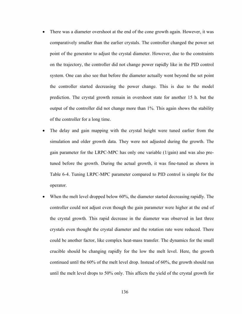
• There was a diameter overshoot at the end of the cone growth again. However, it was
comparatively smaller than the earlier crystals. The controller changed the power set
point of the generator to adjust the crystal diameter. However, due to the constraints
on the trajectory, the controller did not change power rapidly like in the PID control
system. One can also see that before the diameter actually went beyond the set point
the controller started decreasing the power change. This is due to the model
prediction. The crystal growth remain in overshoot state for another 15 h. but the
output of the controller did not change more than 1%. This again shows the stability
of the controller for a long time.
• The delay and gain mapping with the crystal height were tuned earlier from the
simulation and older growth data. They were not adjusted during the growth. The
gain parameter for the LRPC-MPC has only one variable (1/gain) and was also pre-
tuned before the growth. During the actual growth, it was fine-tuned as shown in
Table 6-4. Tuning LRPC-MPC parameter compared to PID control is simple for the
operator.
• When the melt level dropped below 60%, the diameter started decreasing rapidly. The
controller could not adjust even though the gain parameter were higher at the end of
the crystal growth. This rapid decrease in the diameter was observed in last three
crystals even thought the crystal diameter and the rotation rate were reduced. There
could be another factor, like complex heat-mass transfer. The dynamics for the small
crucible should be changing rapidly for the low the melt level. Here, the growth
continued until the 60% of the melt level drop. Instead of 60%, the growth should run
until the melt level drops to 50% only. This affects the yield of the crystal growth for
136

the small diameter crucible. This yield factor should be considered not only during
the required crystal parameter but also during the design of crucible.
• The crystal was pulled out after 30 h growth time. The total weight of the crystal was
210 g. From the grown crystal, the convex shape of the growth interface is can be
observed, which is desirable for the stability of the crystal growth. There was no
crack near the end of the cone growth. In addition, defects were not visible
throughout the crystal length. However, there was a crack in the crystal that was
developed during the cooling cycle of the crystal.
Growth of Crystal-9
-1
-0.5
0
0.5
1
0 300 600 900 1200 1500 1800
Time (minute)
% P
ower
cha
nge
0
15
30
45
60
% D
iam
eter
% Pow er change % Diameter % Diameter SP
Figure 6-13: Diameter and power change graph for Crystal-9
137
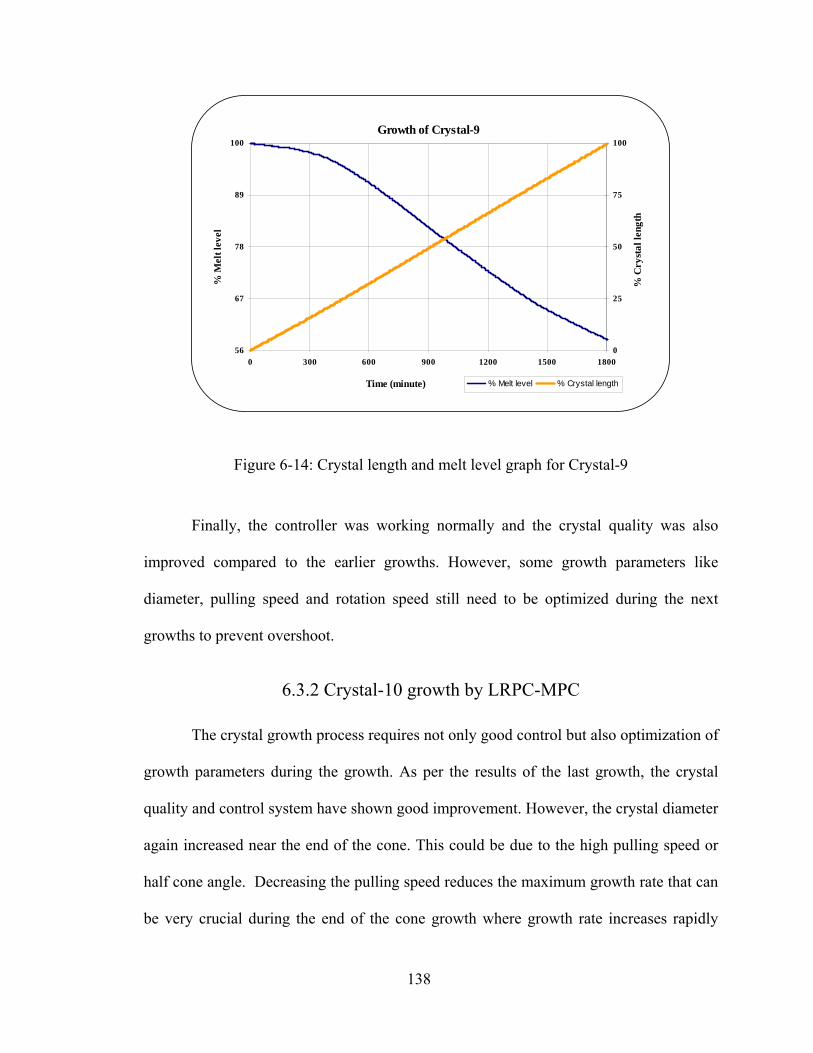
Growth of Crystal-9
56
67
78
89
100
0 300 600 900 1200 1500 1800
Time (minute)
% M
elt l
evel
0
25
50
75
100
% C
ryst
al le
ngth
% Melt level % Crystal length
Figure 6-14: Crystal length and melt level graph for Crystal-9
Finally, the controller was working normally and the crystal quality was also
improved compared to the earlier growths. However, some growth parameters like
diameter, pulling speed and rotation speed still need to be optimized during the next
growths to prevent overshoot.
6.3.2 Crystal-10 growth by LRPC-MPC
The crystal growth process requires not only good control but also optimization of
growth parameters during the growth. As per the results of the last growth, the crystal
quality and control system have shown good improvement. However, the crystal diameter
again increased near the end of the cone. This could be due to the high pulling speed or
half cone angle. Decreasing the pulling speed reduces the maximum growth rate that can
be very crucial during the end of the cone growth where growth rate increases rapidly
138

(exponentially if diameter increases linearly). Decreasing pulling speed also makes the
growth process slower. The total growth time for crystal growth increases. In other
words, controller also gets more time to control process. The higher crystal rotation rate
and crystal cylindrical diameter set point could also be the problem as they define not
only the growth interface but also the heat transfer in the melt and the crystal. Reducing
both should decrease the convection pattern in the melt and could improve the crystal
quality. The stable convection pattern may also help to stabilize the growth even at the
low melt level. In control point of view, varying any of these parameters, including the
pulling speed, does not change the model derived. Hence, the operator does not need to
define the model again. However, fine-tuning may be required.
Figure 6-15 shows Crystal-10 grown using LRPC-MPC technique. Initial process
parameters, calculated parameters and final parameters are shown in Table 6-5. The
pulling speed was decreased to 1.5 mm/h. The power of the cone was increased to 1.6, to
compensate the effect of low pulling speed. The total time for the cone growth was
increased to 10.47 h. with a maximum growth rate of about 6.13 g/h. The total percentage
chemical used dropped to 32.5% as the set point diameter for the cylindrical part was
reduced to 25 mm. The rotation rate was adjusted to 16 rpm.
• The seeding was better than last two times. The seeding diameter was about 4.5 cm.
The length of the seed crystal decreased with every growth. Here, the remaining seed
crystal is kept attached to the original crystal.
139

CGEL
Crystal Growth & Epitaxy LaboratoryAMPAC/UCF
Figure 6-15: Crystal-10 growth by LRPC-MPC
Table 6-5: Process parameter for Crystal-10
Material LGT Growth rate for cylindrical part 6.13 g/hCrucible internal diameter 5.1 mm Total cone growth time 10.47 hInitial weight 515 g Total growth time 35.24 hInitial melt level 41.2 mm Total weight 167.23 gCrystal diameter 25 mm % Chemical used 32.5%Pulling speed 1.5 mm/ h Total calculated length of crystal 72.3 mmRotation speed 16 rpm
Half cone angle 45o Crystal final weight 203 gPower of cone 1.5 Actual Crystal length 110 mmCylindrical crystal length 50 mm Actual growth time 42.4 h
P I 1/LRPC-MPC Initial gain --- --- 800LRPC-MPC After tuning --- --- 700
Controller gains
Calculated parameter before growthInitial parameter
After growth parameter
Gain
Growth parameters for Crystal- 10
140

• The cone growth took about 13 h to end with the final diameter reaching about 8%
higher than set point diameter. The controller was adjusting control signal to change
the power of the generator. Unlike, last experiment, the crystal diameter started
decreasing with the control signal. This indicates that growth parameters were
adjusted near to the optimum values. The overshoot in the diameter may be due to the
half cone angle. Analyzing the last several growths, the cone growth was actually
growing with about 30 degree half cone angle instead of 45 degree. This can be
adjusted during the next growth.
• After 8 h, the controller was able to adjust the crystal diameter near the set point
diameter. The slow response of the controller is mainly due to the two constraints that
were designed in the controller structure. First during the trajectory mapping, a
constraint was put on the maximum rate of change for the diameter. The second
constraint is applied on the rate of change of control signal during the growth. This
helps to protect the control signal going out off bound and having an abnormal jump.
These two constraints also help to conserve the quality of the crystal.
• The crystal was allowed to grow more than the predefined length to see how the
controller behaves with the melt level drop. With the reduced rotation rate, crystal
diameter and pulling speed, the controller was able to maintain the diameter set point
even at low melting level. Unlike earlier growths, diameter did not decreased at the
end of the growth. The growth continued for about 42 h with 40% melt level drop.
• The growth interface was more convex than the last crystal mainly due to the
decrease in rotation rate.
141

Growth of Crystal-10
-1.5
-1
-0.5
0
0.5
375 875 1375 1875 2375 2875
Time (minute)
% P
ower
cha
nge
0
20
40
60
80
% D
iam
eter
% Pow er change % Diameter % Diameter SP
Figure 6-16: Diameter and power change graph for Crystal-10
Growth of Crystal-10
60
74
88
375 875 1375 1875 2375 2875
Time (minute)
% M
elt l
evel
0
25
50
75
100
% C
ryst
al le
ngth
% Melt level % Crystal length
Figure 6-17: Crystal length and melt level graph for Crystal-10
142

From this growth experiment, the optimum growth parameters mainly rotation
rate, diameter set point and pulling speed were achieved. However, to reduce the
diameter overshoot near the cone growth, the half cone angle has to be optimized.
6.3.3 Crystal-11 growth by LRPC-MPC
Figure 6-18 shows Crystal-11 crystal grown using LRPC-MPC technique. Initial
process parameters, calculated parameters and final parameters are shown in Table 6-6.
The half cone angle was reduced to 30 degree to slow the cone growth. The power of the
cone was reduced to 1.4 to compensate the slower cone growth. The total calculated time
for the cone growth was increased to 17.57 h with the maximum growth rate of about
6.13 g/h. The total percentage Chemical used increased to 35% as the cone growth was
extended for about 7 h.
• Again, the seeding was not the idle one. The cone growth continued for about 18 h,
which matched calculated time. i.e. the actual half cone angle was also 30 degree.
• A diameter overshoot was again visible near the end of the cone growth. It decreased
significantly compared to last growths and lasted for only 5 h. This is a significant
improvement. The controller was able to adjust the diameter back to the normal set
point.
• The crystal growth remained stable after the diameter reached back to the set point.
No striation or crack or growth abnormality is visible on the grown crystal.
• The maximum power change was about 0.75% of the seeding power, which is very
small and indicates stable control performance.
143

• The crystal was grown 5 h more than previously calculated, to see how the melt level
drop affects the crystal growth. A small crack on the outside the crystal was observed
due to some impurities in the melt. However, it did not propagate through the crystal.
After all these growth, the performance of the LRPC-MPC controller was
satisfactory. Other crystal growth parameters were also optimized to grow stable small
diameter single crystal.
CGEL
Crystal Growth & Epitaxy LaboratoryAMPAC/UCF
Figure 6-18: Crystal-11 growth by LRPC-MPC
144
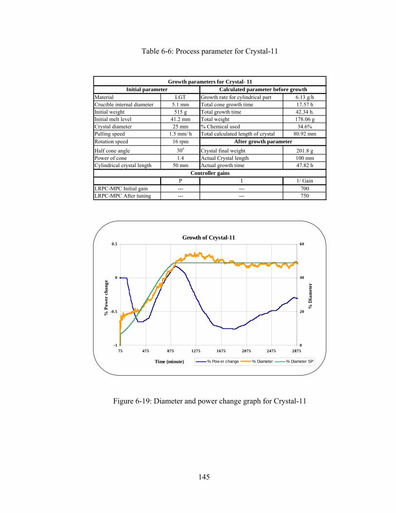
Table 6-6: Process parameter for Crystal-11
Material LGT Growth rate for cylindrical part 6.13 g/hCrucible internal diameter 5.1 mm Total cone growth time 17.57 hInitial weight 515 g Total growth time 42.34 h.Initial melt level 41.2 mm Total weight 178.06 gCrystal diameter 25 mm % Chemical used 34.6%Pulling speed 1.5 mm/ h Total calculated length of crystal 80.92 mmRotation speed 16 rpm
Half cone angle 30o Crystal final weight 201.8 gPower of cone 1.4 Actual Crystal length 100 mmCylindrical crystal length 50 mm Actual growth time 47.82 h
P I 1LRPC-MPC Initial gain --- --- 700LRPC-MPC After tuning --- --- 750
Controller gains
Calculated parameter before growthInitial parameter
After growth parameter
/ Gain
Growth parameters for Crystal- 11
Growth of Crystal-11
-1
-0.5
0
0.5
75 475 875 1275 1675 2075 2475 2875
Time (minute)
% P
ower
cha
nge
0
20
40
60
% D
iam
eter
% Pow er change % Diameter % Diameter SP
Figure 6-19: Diameter and power change graph for Crystal-11
145

Growth of Crystal-11
60
74
88
75 475 875 1275 1675 2075 2475 2875
Time (minute)
% M
elt l
evel
0
25
50
75
100
% C
ryst
al le
ngth
% Melt level % Crystal length
Figure 6-20: Crystal length and melt level graph for Crystal-11
6.3.4 Crystal-12 growth by LRPC-MPC
Once all testing and tuning for the small crystal was over and control system was
satisfactorily stable, it was time to test it for the large diameter (5.1 mm) growth. Figure
6-21 shows Crystal-12 grown using LRPC-MPC technique. The initial process
parameters, calculated parameters and final parameters are shown in Table 6-7.
• The growth parameters like the pulling speed, rotation rate, and half cone angle were
all pre-optimized during earlier growths using the Micricon controller. The
optimization work for large diameter crystal was not related to this study. The
optimum half cone angle is 45 degree. The optimum pulling speed is about 1 mm/h.
The total cylindrical crystal length is 10 cm. The maximum growth rate for the 5.1
mm diameter crystal was 19.31 g/h. The percentage chemical use for large diameter
crystal was about 65% with the approximate weight of 1298 g.
146
• The seeding process for a large diameter crystal is comparatively easier than the small
diameter. This is mainly due to the low convection pattern in the melt and higher
surface area of the melt, which causes a high temperature gradient. Also for the large
diameter crucible, the magnetic coupling frequency for the same temperature is much
lower due the higher crucible surface area for conduction. This makes the power
adjustment easier to control and tune. In addition, the visibility during the seeding is
better than the small diameter crystal. One can see the bright ring around the seed
after the seeding and adjust power before actually pulling the crystal. Here, the
seeding process was like an ideal one and was very stable. The seeding diameter was
around 4 mm.
• The cone growth took about 55 h with about 45 degree half-cone angle. Here, the
crystal was actually following the set point curve throughout the cone growth. In fact,
there was no diameter jump at the end of the cone growth like for the small crystal
growth. It is worth mentioning that the control system, along with cone growth
mapping discussed earlier helped, to reduce the facet formation during the cone
growth and cone was comparatively smoother than the crystal of Figure 2-4.
• The crystal kept growing until at one point a small diameter variation was observed
(at time t=3750 min). The percentage power change (or control signal) was
continuously increasing from cone growth to this moment (time t=3750 min). It also
represents that time delay is changing with the melt level changes.
147

Figure 6-21: Crystal-12 growth by LRPC-MPC
148
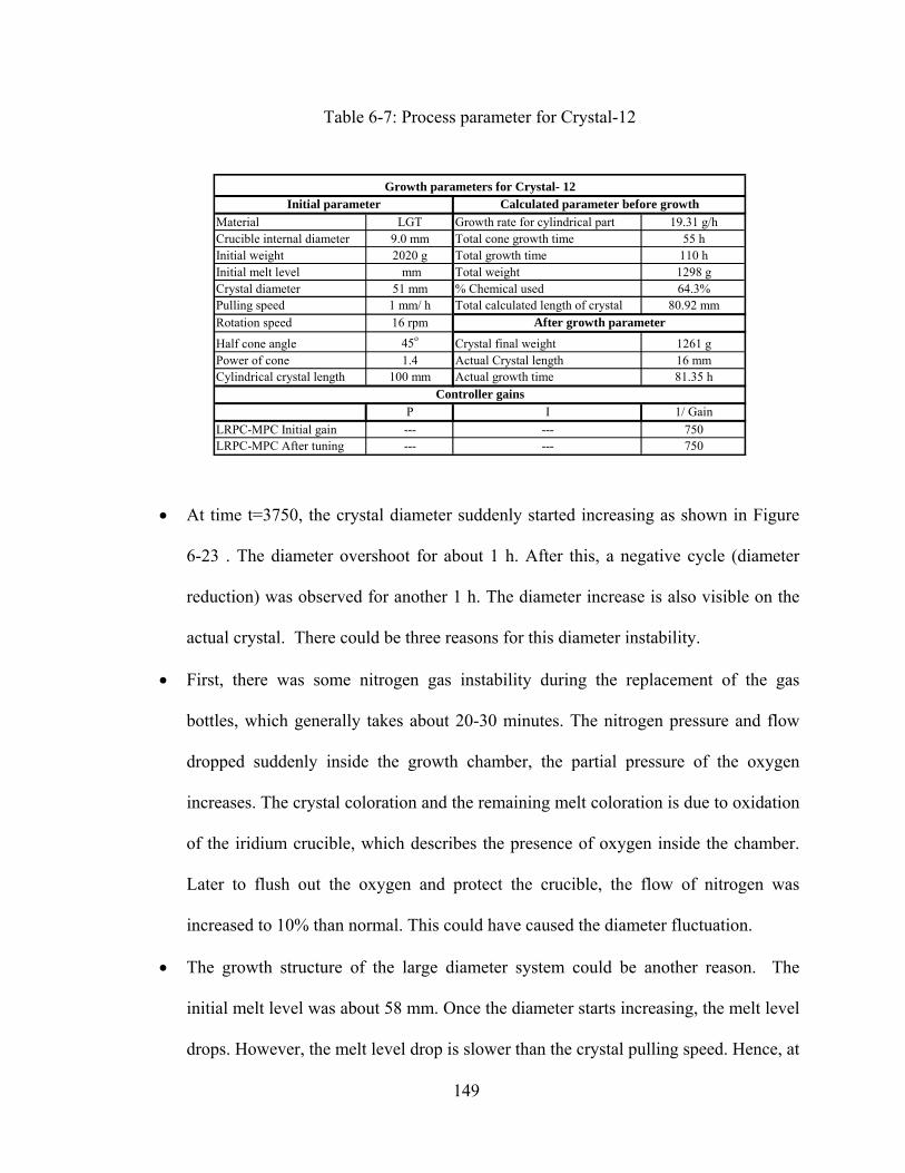
Table 6-7: Process parameter for Crystal-12
Material LGT Growth rate for cylindrical part 19.31 g/hCrucible internal diameter 9.0 mm Total cone growth time 55 hInitial weight 2020 g Total growth time 110 hInitial melt level mm Total weight 1298 gCrystal diameter 51 mm % Chemical used 64.3%Pulling speed 1 mm/ h Total calculated length of crystal 80.92 mmRotation speed 16 rpm
Half cone angle 45o Crystal final weight 1261 gPower of cone 1.4 Actual Crystal length 16 mmCylindrical crystal length 100 mm Actual growth time 81.35 h
P I 1/LRPC-MPC Initial gain --- --- 750LRPC-MPC After tuning --- --- 750
Controller gains
Calculated parameter before growthInitial parameter
After growth parameter
Gain
Growth parameters for Crystal- 12
• At time t=3750, the crystal diameter suddenly started increasing as shown in Figure
6-23 . The diameter overshoot for about 1 h. After this, a negative cycle (diameter
reduction) was observed for another 1 h. The diameter increase is also visible on the
actual crystal. There could be three reasons for this diameter instability.
• First, there was some nitrogen gas instability during the replacement of the gas
bottles, which generally takes about 20-30 minutes. The nitrogen pressure and flow
dropped suddenly inside the growth chamber, the partial pressure of the oxygen
increases. The crystal coloration and the remaining melt coloration is due to oxidation
of the iridium crucible, which describes the presence of oxygen inside the chamber.
Later to flush out the oxygen and protect the crucible, the flow of nitrogen was
increased to 10% than normal. This could have caused the diameter fluctuation.
• The growth structure of the large diameter system could be another reason. The
initial melt level was about 58 mm. Once the diameter starts increasing, the melt level
drops. However, the melt level drop is slower than the crystal pulling speed. Hence, at
149

one point, the crystal starts coming out of the crystal. When it does, the heat transfer
and mass transfer changes dramatically. The heat conduction inside the crystal
increases whereas heat loss from the melt decreases. This could create diameter
instability. Here, when the crystal length was about 75% and the melt level dropped
to about 50%, the grown crystal was actually coming out of the crucible.
• Also, as the melt level drops, total heat conduction from the crucible to melt
decreases. This causes melt to cool down little bit. Generally, the control system
keeps cooling down the crucible to sustain constant diameter for the initial part of the
growth. However, as the melt-level drops and the melt starts cooling down, the
control system starts heating up the generator again at one point. This causes the
change of direction of the control signal as can be seen in the Figure 6-23. At this
point overall control system and growth system is very sensitive to any perturbation.
The melt level at that time was about 50%.
• The controller was able to overcome the diameter instability observed at t=3750
minute. The growth was again stable after that. The crystal was pulled out after 81 h
of growth time.
• There are some cracks at the end of the crystal due to the stresses. Near the end of the
growth, the crystal growth interface was touching at the bottom of the crucible. The
total chemical of 63% was used during the growth. Hence, the remaining melt level
was about 18 mm, which is almost equal to the height of the convex growth interface.
• For the control point of view, the model for prediction, the gain and delay mapping
and the controller gain were kept similar to the last small diameter crystal. The only
parameter changed was as per the Equation (5-2). This is the advantage of x
150

normalizing all parameters insider the control system. In practice, one can grow small
crystal to tune and identify the model of the crystal and apply it to the large diameter
crystal. This could reduce tuning time, the cost of chemical and increase the large
diameter crucible effective life. It is worth mentioning that all of the small crystals
were grown from the old left over chemicals and old polycrystalline crystals. The
large diameter crystal was grown with new chemical.
Growth of Crystal-12
-1
0
1
2
3
4
5
20 820 1620 2420 3220 4020 4820
Time (minute)
% P
ower
cha
nge
0
25
50
75
% D
iam
eter
% Pow er change % Diameter % Diameter SP
Figure 6-22: Diameter and power change graph for Crystal-12
151

Growth of Crystal-12
2.25
2.5
2.75
3
3.25
3350 3550 3750 3950 4150 4350
Time (minute)
% P
ower
cha
nge
52
54.5
57
59.5
62
% D
iam
eter
% Pow er change % Diameter % Diameter SP
Figure 6-23: Diameter and power change graph for Crystal-12 at t=3750 min
Growth of Crystal-12
36
52
68
84
100
20 820 1620 2420 3220 4020 4820
Time (minute)
% M
elt l
evel
0
25
50
75
100
% C
ryst
al le
ngth
% Melt level % Crystal length
Figure 6-24: Crystal length and melt level graph for Crystal-12
152

After, analyzing these three crystals and growing a large diameter crystal using
LRPC-PID, it was clear that the LRPC-MPC technique was better than the conventional
PID control. For the small diameter crystal growth, various growth parameters were
adjusted such that the growth becomes controllable. This is the first time a crystal growth
dynamics was defined as a time varying delayed process. The results are promising and
can lead to further optimization and design of a better control system to improve the
crystal property and the growth performance.
153

CHAPTER 7: CONCLUSION
7.1 Conclusion
The crystal growth by Czochralski growth is a batch process. The process
parameters change as the crystal grows. This is due to the change in heat and mass
transfer dynamics of the growth system as the melt level decreases (or crystal length
increases). These dynamics govern the growth stability and the thermal conditions at the
growth interface, which in turn affects the crystal quality. The optimizations of the
process parameters for such changes are very important for the repeatability and yield of
the crystal.
For slow growing crystals, like LGT studied here, the delay between the system
response and the control signal change is large and cannot be neglected. Conventional
PID control does not consider this delay and creates sluggish response, which is not
suitable for the growth of high-quality oxides. The objective of this work was first to
identify the time delay and then study how this time delay changes as the melt level
decreases and the crystal length increases during the growth. Once this has been
identified, the variable time delay can be incorporated inside the control system by model
prediction technique. Another aspect of the crystal control is to identify the model and
model parameters that can be used for the prediction. Once these parameters are
established, the long range model predictive control system can be designed to grow the
crystals.
This work was divided in three parts:
154

• A few crystals were first grown to study the time delay throughout the crystal growth.
It was found that as the crystal grows and the melt level decreases, the time-delay
between the control signal change and the significant growth response, was
increasing. Hence, the process model can be described as time-varying time delay
model. The effective time delay was found between 8 to 20 minutes, which was later
considered for the control design.
• The data gathered during the growth experiments, were analyzed for order of the
model and the prediction accuracy. The large order model that covers the response
was more accurate than small order model. However, during the real time model
identification, the identification process was unstable for any small perturbation.
Later, only pre-derived model with the suitable order was considered for control
system design.
• The new control systems, LRPC-PID and LRPC-MPC, based on long-range
predictive techniques, were developed and tested in real-time crystal growth. Both
control systems performed satisfactorily after tuning them with delay and gain
mapping. The constraints on the control signal and predictive horizon were also
adjusted for crystal growth stability. At the end, a large diameter crystal was grown
with the same control system to prove its effectiveness for any crystal growth.
It is important to mention that it is the first time that the delay factor was
considered in the control system design for Czochralski crystal growth. In addition, it is
the first time that different control models were compared in a single study and by using
one crystalline material. This did allow to gain extensive knowledge on how and when
the different models can (or cannot) be used. From our experiments, we could
155
demonstrate that the delay in response is a function of time, e.g. time-varying delay. In
the following, the main aspects studied during this work, and main recognitions/results
are summarized:
• The crystal growth was presented as the time-varying time delay process
• The time delay was shown as a function of the melt level or crystal height.
• The order of the process model for the prediction was defined.
• Failure of the real-time model identification process was studied. A pre-derived stable
model was derived from the old growth data for the long range prediction.
• A unit less representation of the process model was derived so that the same control
system could be applied to other diameter crystal growths of the similar material.
• The prediction horizon and mapping of the trajectory for the complete control horizon
were designed. The time delay mapping and gain mapping with respect to crystal
height was also adopted for control system.
• The constraints on the trajectory and control system were applied for stability.
• The lower order model was developed for simulation and pre-tuning of the process.
• The long range model predictive control system was developed using LRPC-PID and
LRPC-MPC technique with time-varying horizon as time delay changes.
• Real-time implementation of the control system for testing and tuning of process
parameter and control parameter was carried out.
7.2 Future work
This work was an initial work towards developing an advanced multiple models,
parameters and constraints based predictive control. For the crystal growth, such
156
controller can not only control the growth process but also helps the operator to optimize
the control to preserve the crystal quality in case of disturbance. The future work topics
are divided in two parts as discussed here:
• Real-time model-identification and control:
a Instead of deriving a complete model during the real-time model
identification, a suitable partial model identification method would be a
better choice to derive a stable model. The model can be bounded in terms
of settling time, stability, gain and other transient response parameters.
These bounds can be calculated from the experiments. These bounds can
change as the melt level changes during the growth and not the whole
model. A recursive estimation of such higher order model with above
bounds would be helpful in many real-time applications other than just a
crystal growth process.
b Such process model can also be represented as a Fuzzy model. The
identification of fuzzy model on real time process would also be a good
area for further research. A fuzzy controller for the long range prediction
and application to crystal growth can also be studied.
c Identification of unknown delay for time-varying delayed process would
also be another topic of research. It has wide a range of applications and
benefits to the control system and modeling area.
• Hysteresis and multiple model, parameter and constraints based predictive control:
a Hysteresis modeling: The crystal growth is a time delayed process. The
heat generation dynamics and the heat loss dynamics creates hysteresis
157

loop in the response. This hysteresis not only changes with the melt level
but also with the input (control signal) of the system. In other words, for
larger input (control signal) the hysterias loop is small where as for small
input, the process has higher hysterias region (wide). The multiple models
of hysteresis for the different melt level and the input could be very
helpful to control the process. Currently, the study of hysteresis system
and control technique is an emerging research area in the control system.
Applying this theory would be beneficial to improve the crystal growth
control.
b Multiple parameters: Instead of presenting growth process as a single
input and single output (SISO) model, other process parameters can be
considered to develop a multi-input and multi-output control system. E.g.
the pulling speed, rotation rate, crucible and crystal temperature, crystal
and crucible position, magnetic field and atmospheric condition. The
multi-input multi-output control system design can be different from the
linear-cascade structure considered in this study.
c Multiple Constraints: The relation of the defect generation and the change
in the temperature could help to develop various constraints that can
minimize these defects. This time only two constraints were tested. The
first one was on the controller speed by the controlling trajectory and the
other one was on the limit of the control system output. Identification of
the other constraints for preserving the quality of the crystal during the
growth would be very important.
158

APPENDIX-A: ELECTRICAL AND INSTRUMENTATION DETAILS
159

The Controller unit is presented in Figure 4-1. Here, the description and setting of
each component of this unit is discussed for the reference. There are mainly for
components of this unit that are two National Instruments card for analog and digital
input and output, motor controller and weight measurement system.
• NI multifunction card: AT-MIO-16E
This E Series device is a configured for an SCXI chassis (DAQ Card), which
houses two other SCXI cards as shown in following figures. The first is SCXI-1121 with
controller block SCXI-1328 for measuring thermocouple temperatures of R.F. Generator
(Device 2, Channel 0) and cooling water system (Device 2, Channel 4) in differential
mode. It also filters out the noise and amplifies the signals as per the preset notches inside
the card.
SCXI-1328
Ch 0
Ch 1
Ch 2
C32+A32-
C26+A26-
C20+A20-
CJC -ThermistorsSetting -Dtemp
Control Temperature
Water Temperature
Spare
SCXI-1121
Ch 0
Ch 1
Ch 2
Ch 4
Gain=100Filter=4MHz
Gain=1000Filter=4MHz
Gain=1000Filter=4MHz
ATMIO-16E-2
MCH0
MCH1
MCH2
MCH4
Device 2Analog input0 to 10 V diff.Channel 0 to 4
SCXI-1181
50 Pin To65 Pin External connector
The E Series device also has two channels of Analog Output (AO) voltage with
selectable reference and range using software. In present configuration, it is used to
control Generator power (Device 2, Channel 1). The control signal is unipolar (0V to
+10V).
• Motor control circuit
160
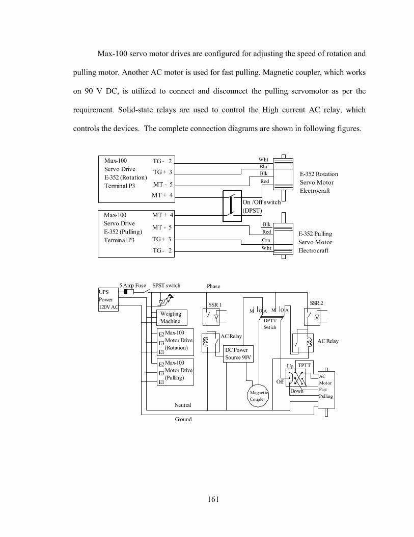
Max-100 servo motor drives are configured for adjusting the speed of rotation and
pulling motor. Another AC motor is used for fast pulling. Magnetic coupler, which works
on 90 V DC, is utilized to connect and disconnect the pulling servomotor as per the
requirement. Solid-state relays are used to control the High current AC relay, which
controls the devices. The complete connection diagrams are shown in following figures.
Max-100Servo DriveE-352 (Rotation)Terminal P3
TG + 3
TG - 2
MT + 4
MT - 5
Max-100Servo DriveE-352 (Pulling)Terminal P3 TG + 3
TG - 2
MT + 4
MT - 5
On /Off switch(DPST)
E-352 RotationServo MotorElectrocraft
E-352 PullingServo MotorElectrocraft
WhtBluBlkRed
BlkRedGrnWht
Up
M O A M O AWeigting Machine
UPS Power120V AC
Max-100 Motor Drive(Rotation)
E1
E2E3
Max-100 Motor Drive(Pulling)
E1
E2E3
DC PowerSource 90V
MagneticCoupler
DPTTSwtich
AC MotorFastPulling
SSR 1 SSR 2
DownOff
TPTT
AC RelayAC Relay
5 Amp Fuse Phase
Neutral
Ground
SPST switch
161

• Connector diagram weighing machine
Digital weight scale is used to measure the weight of crystal. This scale is
connected to computer using RS-232 serial port (No. 0) as shown in the figure with
following configuration. Baud Rate: 1200; Data bits: 7; Stop bits: 0; Parity: 1
Weighing Machine
25 pinserial connector 1
2
3
4
20
7
9 PinSerial Connector(RS-232)Port 0
Computer
8
3
2
20
6
7
Tare command( Symbol/ASCII)ESC T CR LF24 84 13 10
Weight Measurecommand( Symbol/ASCII)ESC P CR LF24 80 13 10
162

APPENDIX-B: ALGORITHEM FOR LRPC MPC TECHNIQUE
163

1 0
,
1. Calculate matraix
for 0 to = Vector
for 0 0
2. Calculate and matraix First row of 0
i i
a i j i j jj j
i
d i
i j
G
i n g a g b
i g
F Gf i
−= =
+
→ = ⇒ = − ⋅ +
→ ∀ < ⇒ =
′
→ ⇒ =
∑ ∑
0, 1
0,
,
for 0 to 1
for
First row of 1 to 1
a a
a j j j
a n n
i j a
j n f a a
j n f a
f i n
+= − ⇒ = −
= ⇒ =
→ ⇒ = −
, 1, 1 1,0
, 1,0 0,
for 0 to 1 ( )
for ( )
3. Calculate matraix
a a
a i j i j
a i n i
d i
0,i j
n
j n f f f
j n f f f
G
− + −
−
+
= − ⇒ = + ⋅
= ⇒ = ⋅
′
→
1,0
for 0
for 1 to b
b
d n
a d n i
i G b
i n G b f −
′= ⇒ =
′→ = ⇒ = ⋅
f
( )
1
10
1 1 1
4. Calcualate matrix: [ ] initialize ( ) ( ) ; ( ) ( )
1 ( ) ( )
for 1,..., with ( 1)
1
a a
T
n j n j
a j
Tj j j j
P P G G Ij j
P k I P k Ij n h k r
P P P h h P h
δ λ
δ α λ λ α
λ λδ
−
− −
−
− − −
= +
→ = =
→ = ⇒ =
→ = + =
→ = − ⋅ ⋅ + ⋅ ⋅
[ ]
1
1
1 1 .. 1 [ ] a
T
⋅
j
Tn
h P
P G G Iδ λ
−
−
−
⋅ ⋅
→ = +
0
5. Calculate matrix : First row of matrix
for 1,...,
a
Tn
i
i j i j aj
K K P
K P g i n−=
G⎡ ⎤= ⎣ ⎦
→ = ⋅ =∑
1 1 1 1
6. Calculating control signal ( ) ( )
( ) ( 1) ( ) a aN Nu k K W f
u k u k u k
δ× ×→ ∆ = −
→ = − + ∆×
164
REFRENCES
[1] DTJ. Hurle, “Crystal Pulling From the Melt”, Springer-Verlay, 1993.
[2] DTJ. Hurle, “Control of Diameter in Czochralski and Related Crystal Growth
Techniques”, Journal of Crystal Growth 42, 1977, Page 473-482.
[3] N. Kobayashi, “Heat Transfer in Czochralski Crystal Growth”. In Preparation and
Properties of Solid State Materials, Ed. WR Wilcox, Dekker, New York, 1981.
[4] B. Chai, J. L. Leafucheur, Y.Y. Ji and H. Qiu, “Growth and Evaluation of Large Size
LGS (La3Ga3SiO14), LGN (La3Ga5.5Nb0.5O14) & LGT (La3Ga5.5Ta0.5O14) Single
Crystal”, IEED International Frequency Control Symposium, 1998, Page 748-760.
[5] Hyoung Jung, Jung Min Ko, Kwang Bo Shim, Tsuguo Fukudu and Keun Ho Auh,
“Influence of Starting Melt Composition on La3(TaxGa1-x)Ga5O15 Crystal Grown by
Czochralski Method”, Journal of Crystal Growth 200, 2000, Page 275-280.
[6] S.V. Tsivinsky, “Dislocation Density in Pure Crystal Grown from Melts”, Kristall
und Technik 10, 1975, Page 5-35.
[7] C.D. Brandle, “Czochralski Growth of Oxides”, Journal of Crystal Growth 264, 2004,
Page 593-604.
[8] M.A. Gevelber and G. Stephanopoulos, “Dynamics and Control of the Czochralski
Process-І”, Journal of crystal growth 84, 1987, 647-668.
[9] M.A. Gevelber, G. Stephanopoulos and M.J.Wargo, “Dynamics and Control of the
Czochralski Process-ІІ”, Journal of crystal growth 91, 1988, 199-217.
[10] M.A. Gevelber, M.J. Wargo and G. Stephanopoulos, “Advanced Control Design
Considerations for the Czochralski Process”, Journal of crystal growth 85, 1987, 256-
263.
165

[11] DTJ Hurle, “Dynamics, Stability and Control of Czochralski Growth”, Journal of
Crystal Growth 128, 1993, Page 15-25.
[12] J.P. Wilde, Lamberturs Hesselink and Robert S. Feigelson, “Diameter Stabilization of
Czochralski-grown Sr0.61Ba0.39Nb2O6 (SBN) Crystals Using Real-time Computer
Control”, Journal of Crystal Growth 113, 1991, Page 337-359.
[13] M.D. Aggarwal, R. Metzl, W.S Wang and J. Choi, “A Versatile Czochralski Crystal
Growth System with Automatic Diameter Control”, Review of Scientific Instruments
66, n 7, July 1995, Page 3939-3942.
[14] M. Malek-Zavarei and M. Jamshidi, “Time-Delay Systems: Analysis, optimization
and applications”, North-Holland Systems and Control series – 9, Elsevier Science
publishing, Netherland, 1987.
[15] P.B. Deshpande and R.H. Ash, “Elements of Computer Process Control”, ISA, 1981.
[16] E.F. Camacho and C. Bordons, “Model Predictive Control in the Process”, Springer-
verlay, 1995.
[17] K.J. Åström, and B. Wittenmark, “Adaptive Control”, Addison - Wesley,
Massachusetts, 1989.
[18] L. Ljung, “System Identification: Theory for the User”, Printice-Hall, Englwood
cliffs, N.J., 1987.
[19] G. Favier, D. Dubois and C. Rougerie, “A Review of k-step ahead Predictors”, IFAC
Proceeding on System Identification Parameters Estimation 2, 1988, Page 887-893.
[20] D.W. Clarke, C. Mohtadi and P.S. Tuffs, “Generalized Predictive Control Part 1 and
2”, Automatica 23-2, 1987, Page 137-160.
166

[21] D.W. Clarke, “Advances in Model-based Predictive Control”, Oxford University
Press, Oxford, 1994.
[22] J.R. Gossner, B. Kouvaritakis and J.A. Rossiter, “Stable Generalized Predictive
Control with Constraints and Bounded disturbances”, Automatica 33, 1997, Page
681-700.
[23] T. Alvarez and C. Panda, “Handling Infeasibility in Predictive control”, Computers
and Chemical engineering 21, 1997, Page 577-582.
[24] R.M.C De Keyser, Ph. G.A. Van de Velde and F.G.A Dumortier, “A Comparative
Study of Self-adaptive Long Range Predictive Control Methods”, Automatica 24-2,
1988, Page 149-163.
[25] R.M.C. De Keyser and A. Van Cauwenberghe, “Extended Prediction Self-adaptive
Control”, IFAC Symposium on Identification and System Parameter Estimation”,
1985, Page 1255-1260.
[26] D.W. Clarke and L. Zhang, “Long-range Predictive Control using Weighting-
sequence Model”, Proceeding IEE – 134, Pt-D, 1987, Page 187-195.
[27] W. Bardsley, G.W. Green, C.J. Holliday and DTJ Hurle, “The Weighing Method of
Automatic Czochralski Crystal Growth-I”, Journal of Crystal Growth 40, 1977, Page
13-20.
[28] W. Bardsley, G.W. Green, C.J. Holliday and DTJ Hurle, “The Weighing Method of
Automatic Czochralski Crystal Growth-II”, Journal of Crystal Growth 401, 1977,
Page 21-28.
167
[29] G.C. Joyce, DTJ Hurle and Q.A.E. Vaughan, “Novel Development of the Weighting
Method for Automatic Czochralski Crystal Growth of Semiconductors”, Journal of
Crystal Growth 100, 1990, Page 11-25.
[30] Nikolai V. Abrosimov, Vladimir. N. Kurlov and Sergei. Rossolenko, “Automated
Control of Czochralski and Shaped Crystal Growth Process using Weighing
Techniques”, Progress in Crystal Growth and Characterization of Materials, 2003,
Page 1-57.
[31] DTJ Hurle, G.C. Joyce, M. Ghassempoory, A.B. Crowely and E.J. Stern, “The
Dynamics of Czochralski Growth”, Journal of Crystal Growth 100, 1990, Page 11-25.
[32] J.J. Derby and R.A. Brown, “On the Dynamics of the Czochralski Crystal Growth”,
Journal of Crystal Growth 83, 1987, Page 137-151.
[33] Roberto Irizarry-Rivera and Warren Seider, “Model-predictive Control of the
Czochralski Crystallization Process”, Journal of Crystal Growth 178, 1997, Page 593-
633.
[34] Michael Gevelber, Danielle Wilson and Ning Duanmu, “Modeling Requirements for
Development of an Advanced Czochralski Control System”, Journal of Crystal
Growth 230, 2001, Page 217-223.
[35] Antonios Armaou and Panagiotis Christofides, “Crystal Temperature Control in the
Czochralski Crystal Growth Process”, Process System Engineering, AIChE Journal
47, n-1, January 2001, Page 79-106.
[36] Haihong Qiu, “Development of a Computer Control System with Self-tuning Growth
Rate Control for the Czochralski Crystal Growth Process”, PhD Thesis, University of
Central Florida, 1997.
168

[37] J.J. Derby and R.A. Brown, “Thermal-Capillary Analysis of Czochralski and Liquid
Encapsulated Czochralski Crystal Growth”, Journal of Crystal Growth 75, 1986, Page
227-240.
[38] K. Rieding, “Autonomous Liquid Encapsulated Czochralski Growth of Single Crystal
GaAs by Intelligent Digital Control”, Journal of Crystal Growth 89, 1988, Page 435-
446.
[39] Peter Sveshtarov and Marvin Gospodinov, “The Effect of the Interface Shape on
Automatic Czochralski Weight Diameter Control System Performance”, Journal of
Crystal Growth 113, 1991, Page 186-208.
[40] S.H. Lee, V.J. Kim, S.H. Cho and E.P. Yoon, “The Influence of the Czochralski
Growth Parameters on the Growth of Lithium Niobate Single Crystals”, Journal of
Crystal Growth 125, 1992, Page 175-180.
[41] Christine Klemenz, Jun Luo and Dhaval Shah, In: 29th International Conference on
Advanced Ceramics and Composites, Cocoa Beach FL, 2005.
[42] J. Luo, D. Shah, C.F. Klemenz, M. Dudley, H. Chen, Journal of Crystal Growth 287
(2006) p. 300-304.
[43] Dhaval S. Shah and Christine F.Klemenz, In: IEEE International Frequency Control
Symposium (2006) p. 196-200.
[44] H. Stao, M. Kumatoriya and T. Fujii, “Control of the Facet Plane Formation on Solid-
Liquid Interface of LGS”, Journal of Crystal Growth 242, 2002, Page 177-182.
[45] Dhaval S. Shah, “Application of Model Reference Adaptive Control for Czochralski
Crystal Growth Technique”, MS Thesis, University of Central Florida, 2004.
169
[46] M.S. Grewal and A.P. Andrews, “Kalman Filtering: Theory and Practice”, Printice
Hall, Englwood Chiffs, NJ, 1993.
[47] H. Akaike, “A New Look at Statistical Model Identification”, IEEE Transaction on
Automatic Control 19, no 6, 1974, Page 716-723.
[48] G. Schwarz, “Estimating the Dimension of a Model”, Analytical Statistics 6, no-2,
1978, Page 461-464.
[49] Sarkar, P.P. Kanjilal, “On a Method of Identification of Best Subset Model from Full
AR Model”. Communications in Statistics –Theory and Methods – 24, No-6, Page
1551-1567.
[50] P. Young, “Recursive Estimation and Time Series Analysis, an Introduction”,
Springer-verlag, Berlin, 1984.
[51] R.R. Hocking, “Development in Linear Regression Methodology 1959-1982”,
Technomatrics-25, no 3, 1983, Page 219-249.
[52] S. Boyd, L El Ghaouni, E. Feron and V. Balakrishnan, “Linear Matrix Inequalities in
Systems and Control Theory”, SIAM books, 1994.
[53] G.J. Bierman, “Factorization Method for Discrete Sequential Estimation”, Academic
Press, New York, 1977.
[54] Wai Gao, Miao Lei Zhou, Yuan Chun Li and Tao Zhang, “An Adaptive Generalized
Predictive Control of Time-Varying Delay System”, Proceeding of the Third
International Conference on Machine learning and Cybernetics, Shanghai, 26-29,
August 2004, Page 878-881.
[55] Zheng and Feng, “Identification of Stochastic Time Lag Systems in the Presence of
Colored Noise”, Automatica 26, 1990, Page 769-779.
170