1

Delineating Lake Drainage Basins in GIS Prepared by Thomas J. Ballatore, Ph.D. Director, Lake Basin Action Network (LBAN) Affiliated Scientist, Center for Ecological Research, Kyoto University Visiting Researcher, International Lake Environment Committee (ILEC) Foundation Please send questions and comments to ballatore@lakebasin.org

Purpose This tutorial provides a step-by-step guide for delineating lake drainage basins using geographic information system (GIS) software. It uses the Lake Biwa drainage basin as an example but the techniques presented here are fully applicable to lakes in any country you might be working on.

Advice Using GIS software is much easier than it was in the past. Also, the burden of collecting, scanning and otherwise processing data for use in GIS has been greatly reduced by the many fine and free global data sets that have become available in recent years. Nevertheless, delineating a drainage basin of interest to you will not be an easy task. I have tried to make this tutorial as simple yet complete as possible but, in general, using GIS software requires good computer skills and a lot of patience. The software we will use (ArcGIS) is not bug free and crashes often. Make sure to save your data often. Once you complete this tutorial, I encourage you to try the same for a drainage basin you are working on. Feel free to contact me by e-mail anytime. I am quick to respond and enjoy learning about new cases all the time!

What you need

• ArcGIS (version 9.0 and above; ArcView license level is fine) with the Spatial Analyst Extension installed and running on your computer. Six-month trail versions are available with many of the ESRI ArcGIS guidebooks including titles such as “GIS Tutorial: Workbook for ArcView 9, Third Edition”, ISBN 9781589482050. The list price is $79.95 but new copies are available at Amazon.com for around $50. You may also contact ESRI at www.esri.com directly for a trial version.

• Note that a newer version of ArcGIS software (currently 10.1) is available but the interface is significantly different from the version used here (9.3). Please send me an e-mail if you are using 10.0 or 10.1 and cannot find tools described here.

• Internet access (for downloading files and for optionally using Google Earth). • All of the data used in this tutorial are available free of charge from their respective

sources. Links are given at the appropriate places below.

2

Preliminaries

Step 1. Establishing a File System for your GIS Work You will be downloading many files and producing even more. A good file management structure is crucial to keep track of everything. There are many possible structures for this, but I recommend the following one and will use it in this tutorial. Later on, feel free to devise a different structure if you like but always remember to give sensible file names to your products and to delete the temp files regularly.

1. On the C: drive, make a folder called GIS, i.e., C:\GIS 2. Inside the GIS folder, make three folders called Basins, Data, and Temp, i.e.,

C:\GIS\Basins, C:\GIS\Data, C:\GIS\Temp 3. Within Basins, create a folder called Biwa, i.e. C:\GIS\Basins\Biwa 4. Within Biwa, make a folders called SWBD and SRTM3, i.e.

C:\GIS\Basins\Biwa\SWBD, and so on. 5. Within Data, make three folders called SWBD and SRTM3, i.e. C:\GIS\Data\SWBD,

and so on. Some notes:

• You do not have to use the root C: drive but we will for this tutorial. I find that processing is faster if done on the C:, in particular if the files of interest are not buried in too many folders.

• It is good practice to NOT use spaces in your folder names. The latest ArcGIS versions seem to have no problem with spaces but older versions did. To be safe, no spaces! Same with file names.

Step 2. Starting ArcMap and Making Basic Settings The software we are using is called ArcGIS and is made by a company called ESRI. There are three important distinctions to understand about ArcGIS:

1. License level. The tools available within ArcGIS depend on the license level. Basic is called ArcView, Intermediate is called ArcEditor, and Advanced is called ArcInfo. Our trial versions are for the ArcView license level, and although you may instinctually want to have the complete ArcInfo version, it is very rare that you’ll actually make use of the extra tools it contains. For our purposes, ArcView is more than enough.

2. Extensions. In addition to the license level distinction, ArcGIS also comes with a choice of extensions which extend the functionality of the basic program. For example for work, we need tools that are contained in the Spatial Analyst extension. Other extensions include 3D Analyst, Geostatistical Analyst, Maplex and so on. Fortunately, the trial version comes with all extensions including the required Spatial Analyst.

3. ArcMap vs. ArcCatalog. Within all license levels of ArcGIS, you will find two separate programs. ArcMap is the main program we use for analysis and mapping. ArcCatalog is used for file management. It is similar to Windows Explorer but is

3

optimized for geographic data. Both contain the ArcToolbox. As you can see, the names get a little confusing but with some experience, you will have no problems.

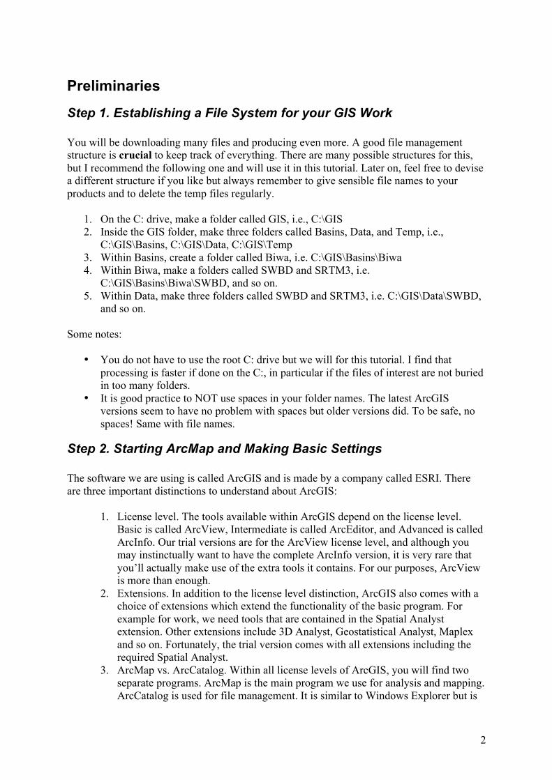
Start ArcMap. You can do this by clicking on Windows Start Menu | All Programs | ArcGIS | ArcMap. After the startup splash screen finishes, you will see something like the following:

If you do not see some of the tool bars, just right click on the Menu bar (the one that contains the words “File” etc. and toggle on Spatial Analyst, Tools and whatever others you wish you use. If ArcToolbox is not showing by default in ArcMap, either click the ArcToolbox icon on the main menu toolbar, or choose Window | ArcToolbox on the very top menu to make it appear. Let’s immediately do two things. First, click File | Save As and save the map as “Biwa.mxd” to the C:\GIS\Basins\Biwa folder. I will not mention it again, but save the document regularly! Next, click File | Document Properties and click on the Document Source Properties button. You get the following dialog:

4

Choose “Store relative path names to data sources” and make this your default. This option allows you to move your GIS folder to a differently named hard disk without breaking the links to your data. This illustrates an important point about ArcMap; namely, the ArcMap document (Biwa.mxd in this case) does not contain the actual data but rather it contains information about how to display data that exist on your hard drive (or on a server or anywhere except in the .mxd file which cannot contain the actual data). This point will become clear by the end of the tutorial, but you need to remember that you cannot give just give someone the .mxd file and expect them to get the map you have made because the data will be in a different place (in this case, in the folder C:\GIS\Basins\Biwa).

Step 3. Deciding what data are necessary, i.e. Where is your basin? There are many ways you could delineate a given lake’s drainage basin. You could:

1. Use a printed topo map and judge from the contours where water is likely to flow; 2. Roughly sketch the same by looking at a remotely sensed image; or 3. Use digital elevation data in a GIS.

The last one is the technique we will use and is by far the easiest and most replicable. You can think of options (1) and (2) like writing an essay by hand and (3) like using a word processor. Figuring out the extent you need to cover (the range of data in lat/long), however, is tricky because you need to obviously have enough to cover the whole drainage basin but you don’t want to have too much extra because that slows processing time. In other words, you need to have a rough idea where your drainage basin is before you actually delineate it with precision!

5

You might already have drainage basin maps that give you a good idea, or you might simply have first-hand knowledge that allows you to make a sensible guess. One technique that I often use when working with drainage basins I am not very familiar with is to:

1. Open Google Earth (available for free at http://www.google.com/earth/index.html) 2. Make sure the Latitude/Longitude grid is turned on (usually Cntl+L) 3. Zoom to the area of interest and look at the topography and rivers and make an

estimate of the North-South-East-West extents that would enclose the basin comfortably.

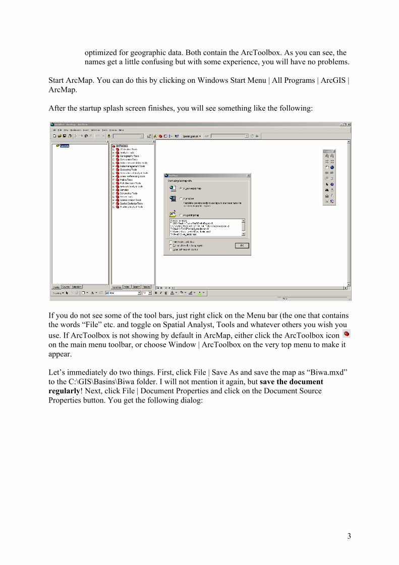
4. You might want to use the Add Polygon or Add Path tool to leave a record of your tracing. An example for the Lake Biwa basin is given below.

I made that by just looking at mountains and rivers and roughly estimating the limits of the drainage basin. (I’ve zoomed out so you can see the lat/long better but naturally zoomed in when tracing it.) In terms of latitude and longitude, the basin is probably completely within by a polygon from E135~E137 and N34~N36.

Working with Features/Vectors There are two major types of data that are used in a GIS: features and rasters. Features, sometimes called vectors, are like the fonts on your computer screen: no matter how much you zoom in, they are always “crisp”. This is because they are drawn based on mathematical rule governing their shape. On the other hand, rasters are like a photograph: they are made up of individual pixels. If you zoom in, you will see a “jagged” look. Their resolution depends on your camera and on the way you might have processed the image.

6

They have complementary strengths and are ubiquitous in modern GIS analysis like the kind in this tutorial. It is possible to convert one to the other and back, and sometimes we will do that, but in general we let features be features and rasters be rasters.

Step 4. Downloading Waterbody Features Before we start working with the elevation data, it is nice to have a view of the waterbody locations in our target area. One of the best global-scale data sets for waterbodies is NASA’s Shuttle Radar Topography Mission (SRTM) Water Body Dataset, known as SWBD, which shows the location of water bodies during a February 2000 Shuttle mission that were greater than approximately 600m in height and 183m in width. You can download this data from: http://dds.cr.usgs.gov/srtm/version2_1/SWBD/ The files we want are in the SWBD_east folder. The files contain data on 1x1 degree tiles and area named based on the coordinates of their lower left corner (southwest). For the Lake Biwa basin, let’s use the following 4 tiles: e135n34e.zip e135n35e.zip e136n34e.zip e136n35e.zip These correspond to the nine tiles we identified in the Google Earth exercise above. Note that the “e” before .zip represents “Eurasia” for these tiles. For other regions of the world, the letter used is different (e.g. “s” for South America”). Make a new folder called C:\GIS\Data\SWBD and save these 4 files there. Then, make a new folder called C:\GIS\Basins\Biwa\SWBD and unzip them there. You should end up with something that looks like this depending on your Windows version and display preferences:

7

Notice that each file when unzipped becomes 3 distinct files: .dbf file, .shp file and .shx file. This set forms what is called a shapefile (a feature/vertor file) and illustrates one of the difficult parts of working with GIS as compared with other programs such as, say, Microsoft Excel. Let’s say you want to share the e135n34e shapefile with a colleague. If you copy only e135n34e.shp and forget e135n34e.dbx and e135n34e.shx, the file will not be readable. You need to be either very careful about this, or use an application called ArcCatalog (part of ArcGIS).

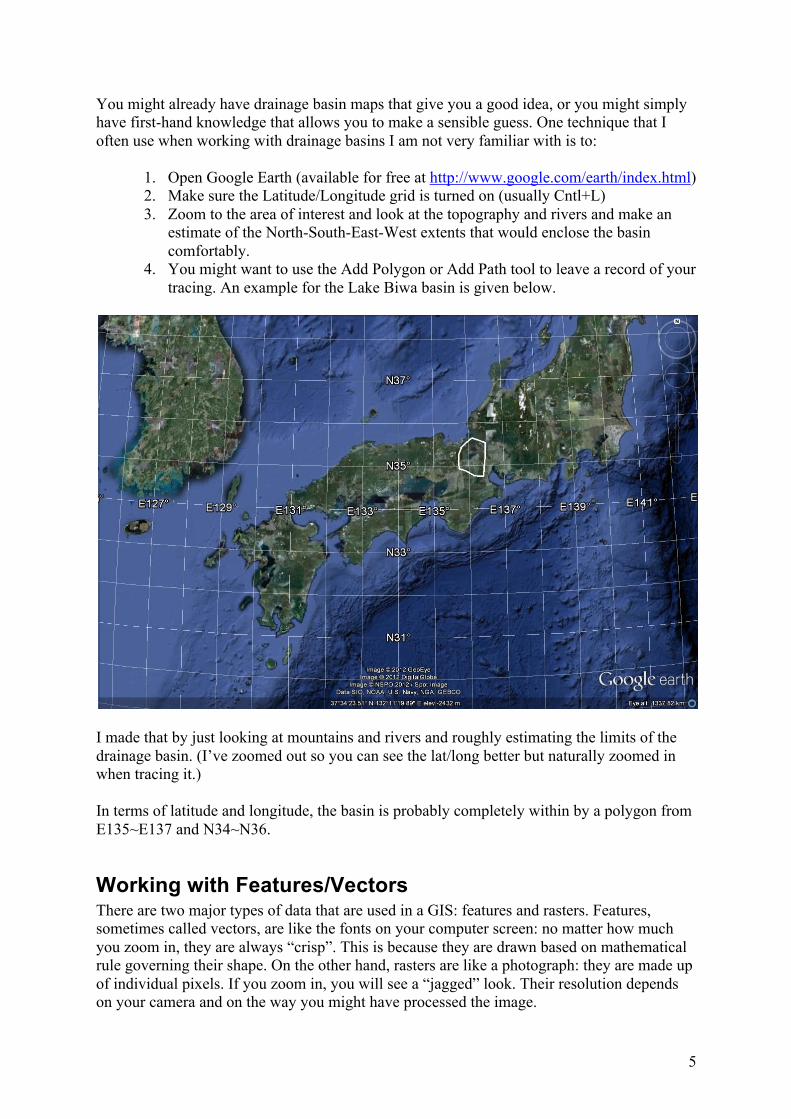
Step 5. Adding and Manipulating SWBD shapefiles in ArcMap 5.1 Define Coordinate System. Before we can add the SWBD waterbody files we unzipped above, we need to define the coordinate system they are using. From the SWBD readme file, we know that the data is in the Geographic Coordinate System (GCS) with the datum (shape of the earth) WGS_1984. We will use a tool in the ArcToolbox to do this. In ArcToolbox, go to Samples | Data Management | Projections and double click Batch Define Coordinate System. In the dialog opens, click on icon, navigate to C:\GIS\Basins\Biwa\SWBD and add the 4 files (note that ArcMap displays only the 4 “set of three” files and not the total 12 individual ones that you see in Windows Explorer). Next, click the icon. You will get the following dialog. Click on Select, and navigate to Geographic Coordinate Systems | World | WGS_1984 (see figure) and click Add, then OK.

You should see the following:

8

Select OK. The tool runs. You will see the following dialog (which may close automatically if you have selected that option).

The tool executed successfully but nothing “happened” in the ArcMap window. However, if you use Windows Explorer to look in C:\GIS\Basins\Biwa\SWBD, you’ll see that some new files have been created, namely a .prj (projection) file for each of the 9 shapefiles as well as some .xml files. The .prj file can be opened in Notepad. The contents look like this:

These are the parameters we specified in the Batch Define Coordinate System tool. The SWBD files are not ready to add to ArcMap. (Note that because we had 4 files, we used the Batch Define Coordinate System tool. Alternatively, we could have gone in the ArcToolBox to Data Management Tools | Projections and Transformations | Define Projection, and achieved the same result, albeit requiring us to run the tool 4 times. Also, we could have simply made the .prj files in notepad! This highlights a key aspect of using GIS well: you should be able to think of several ways of accomplishing the same task---just in case one of the methods doesn’t work.)

9

5.2 Add SWBD files. Next, click the Add Data icon and navigate to the SWBD files. Select all as follows:

then click Add. You will now see something like the following:

Lake Biwa is clearly visible, as are Ise Bay (southeast), Osaka Bay (southwest) and the Sea of Japan (northwest). Note that when shapefiles are added to ArcMap, they are given a random color from the default pastel palette; therefore, the colors you see will likely be slightly different. 5.3 Merge the files. Right now, we have 4 separate files. Lake Biwa itself is divided among four of them. Ideally, we’d like to have each waterbody as an independent “record” within a single shapefile. This is a several-step process. First, in ArcToolBox, go to Data Management Tools | General | Merge and open the tool. Add the four SWBD shapefiles, and make the output file name SWBD_Merge.shp. It should look like this:

10

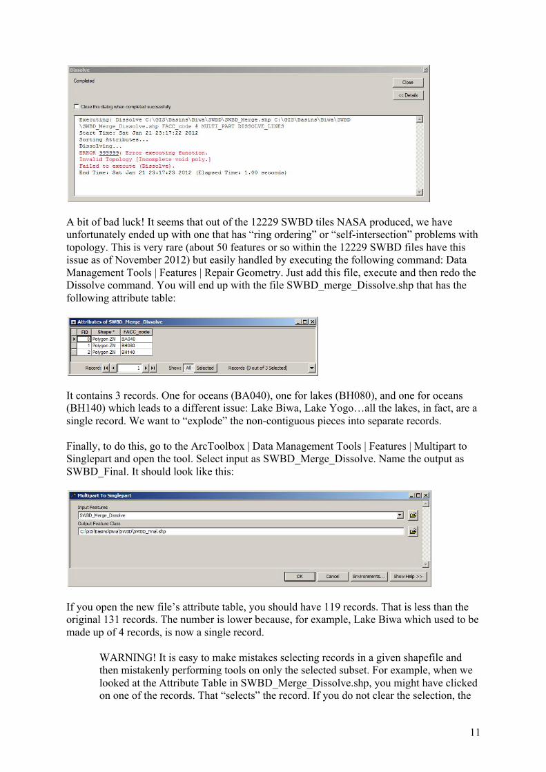
Click OK. A new shapefile is added to the map. It contains all the records from the other four shapefiles in a single file and the colors are the same now. However, Lake Biwa (as well as many other waterbodies) is still split over multiple records. You can see this if you right click on the new shapefile’s layer and choose Attribute table. There are a total of 131 records in this file. Each is a polygon that you could select in the map. Some, like Lake Biwa’s four polygons, area contiguous but not yet connected into one. Next, let’s “merge” all the independent records together. Go to Data Management Tools | Generalization | Dissolve. Add SWBD_Merge.shp. Name the new file as SWBD_Merge_Dissolve. Make sure that you select FACC_CODE in the Dissolve Fields box. This ensures that the three waterbody types in this feature (rivers, lakes and oceans) are dissolved with similar types. It should look like this:

Click OK and get an…ERROR! At least I get an error on my version. The following dialog appears:

11

A bit of bad luck! It seems that out of the 12229 SWBD tiles NASA produced, we have unfortunately ended up with one that has “ring ordering” or “self-intersection” problems with topology. This is very rare (about 50 features or so within the 12229 SWBD files have this issue as of November 2012) but easily handled by executing the following command: Data Management Tools | Features | Repair Geometry. Just add this file, execute and then redo the Dissolve command. You will end up with the file SWBD_merge_Dissolve.shp that has the following attribute table:

It contains 3 records. One for oceans (BA040), one for lakes (BH080), and one for oceans (BH140) which leads to a different issue: Lake Biwa, Lake Yogo…all the lakes, in fact, are a single record. We want to “explode” the non-contiguous pieces into separate records. Finally, to do this, go to the ArcToolbox | Data Management Tools | Features | Multipart to Singlepart and open the tool. Select input as SWBD_Merge_Dissolve. Name the output as SWBD_Final. It should look like this:

If you open the new file’s attribute table, you should have 119 records. That is less than the original 131 records. The number is lower because, for example, Lake Biwa which used to be made up of 4 records, is now a single record.

WARNING! It is easy to make mistakes selecting records in a given shapefile and then mistakenly performing tools on only the selected subset. For example, when we looked at the Attribute Table in SWBD_Merge_Dissolve.shp, you might have clicked on one of the records. That “selects” the record. If you do not clear the selection, the

12

following tool will only operate on the selected records. I make this mistake all the time! To select and unselect, you can use the following icons in the Tools toolbar, and , respectively.

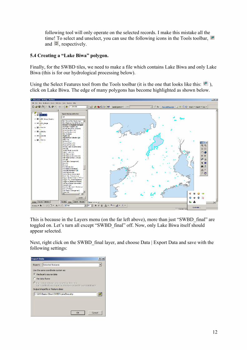
5.4 Creating a “Lake Biwa” polygon. Finally, for the SWBD tiles, we need to make a file which contains Lake Biwa and only Lake Biwa (this is for our hydrological processing below). Using the Select Features tool from the Tools toolbar (it is the one that looks like this: ), click on Lake Biwa. The edge of many polygons has become highlighted as shown below.

This is because in the Layers menu (on the far left above), more than just “SWBD_final” are toggled on. Let’s turn all except “SWBD_final” off. Now, only Lake Biwa itself should appear selected. Next, right click on the SWBD_final layer, and choose Data | Export Data and save with the following settings:

13

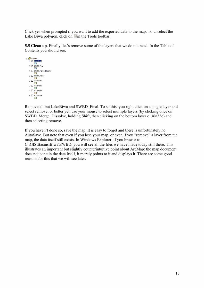
Click yes when prompted if you want to add the exported data to the map. To unselect the Lake Biwa polygon, click on in the Tools toolbar. 5.5 Clean up. Finally, let’s remove some of the layers that we do not need. In the Table of Contents you should see:

Remove all but LakeBiwa and SWBD_Final. To so this, you right click on a single layer and select remove, or better yet, use your mouse to select multiple layers (by clicking once on SWBD_Merge_Dissolve, holding Shift, then clicking on the bottom layer e136n35e) and then selecting remove. If you haven’t done so, save the map. It is easy to forget and there is unfortunately no AutoSave. But note that even if you lose your map, or even if you “remove” a layer from the map, the data itself still exists. In Windows Explorer, if you browse to C:\GIS\Basins\Biwa\SWBD, you will see all the files we have made today still there. This illustrates an important but slightly counterintuitive point about ArcMap: the map document does not contain the data itself, it merely points to it and displays it. There are some good reasons for this that we will see later.

14

Working with Rasters Now that we have (1) some experience with ArcMap and working with features like shapefiles and (2) confirmed that our estimate of the Lake Biwa basin is reasonable (the 4 SWBD tiles appear to be sufficient), we will add elevation data to the map and delineate the drainage basin. Elevation data may be in the form of features such as contours, but we will use a raster. This is a compact format for this data type and it allows us to use the ArcGIS hydrology tools for delineation.

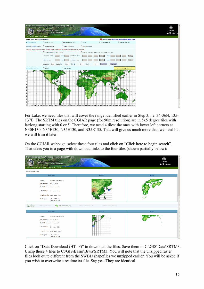
Step 6. Downloading Elevation Data In this example, we use the 3-arc second Shuttle Radar Topography Mission (SRTM3) Digital Elevation Model (DEM) data collected in February 2000 by NASA. This is currently the highest-quality, highest-resolution, global-coverage (60°N-56°S) DEM available (for free, too!). At the equator, the resolution is approximately 90m which is sufficient for our purpose. A general description of the data is at: http://www2.jpl.nasa.gov/srtm/cbanddataproducts.html If you like you can download individual 1x1 degree tiles at http://dds.cr.usgs.gov/srtm/version2_1/SRTM3/ but while the tiles available there are very useful (and the ones I usually use for my own work), they need some special processing (creating of header files, interpolation of nodata areas, etc.) that make them difficult for GIS beginners to use. Therefore, in this tutorial, we will use an SRTM-based dataset that has already been processed and put into convenient 5x5 degree tiles. These are available at: http://srtm.csi.cgiar.org/SELECTION/inputCoord.asp (You can find a description of the data as well as elevation available at lower resolutions such as 250m, 500m, and 1km at http://srtm.csi.cgiar.org/) The data selection page is below. In my experience, choosing the “Harvest Choice” server has led to faster downloads. Also, you have a choice of downloading the data as “GeoTiff” or “ArcInfo ASCII”. The GeoTiff files are easier to use for our work so please select that button. To select the actual tiles, just click on the map with your mouse. I find that the selection (at least on my computer) has a slight bug…to select a given tile, click on the tile BELOW the one you want.

15

For Lake, we need tiles that will cover the range identified earlier in Step 3, i.e. 34-36N, 135-137E. The SRTM tiles on the CGIAR page (for 90m resolution) are in 5x5 degree tiles with lat/long starting with 0 or 5. Therefore, we need 4 tiles: the ones with lower left corners at N30E130, N35E130, N35E130, and N35E135. That will give us much more than we need but we will trim it later. On the CGIAR webpage, select these four tiles and click on “Click here to begin search”. That takes you to a page with download links to the four tiles (shown partially below):

Click on “Data Download (HTTP)” to download the files. Save them in C:\GIS\Data\SRTM3. Unzip those 4 files to C:\GIS\Basin\Biwa\SRTM3. You will note that the unzipped raster files look quite different from the SWBD shapefiles we unzipped earlier. You will be asked if you wish to overwrite a readme.txt file. Say yes. They are identical.

16

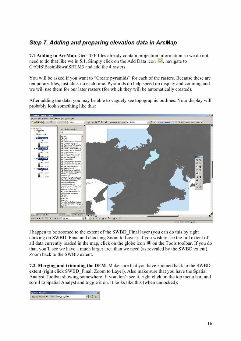
Step 7. Adding and preparing elevation data in ArcMap 7.1 Adding to ArcMap. GeoTIFF files already contain projection information so we do not need to do that like we in 5.1. Simply click on the Add Data icon , navigate to C:\GIS\Basin\Biwa\SRTM3 and add the 4 rasters. You will be asked if you want to “Create pyramids” for each of the rasters. Because these are temporary files, just click no each time. Pyramids do help speed up display and zooming and we will use them for our later rasters (for which they will be automatically created). After adding the data, you may be able to vaguely see topographic outlines. Your display will probably look something like this:

I happen to be zoomed to the extent of the SWBD_Final layer (you can do this by right clicking on SWBD_Final and choosing Zoom to Layer). If you wish to see the full extent of all data currently loaded in the map, click on the globe icon on the Tools toolbar. If you do that, you’ll see we have a much larger area than we need (as revealed by the SWBD extent). Zoom back to the SWBD extent. 7.2. Merging and trimming the DEM. Make sure that you have zoomed back to the SWBD extent (right click SWBD_Final, Zoom to Layer). Also make sure that you have the Spatial Analyst Toolbar showing somewhere. If you don’t see it, right click on the top menu bar, and scroll to Spatial Analyst and toggle it on. It looks like this (when undocked):

17

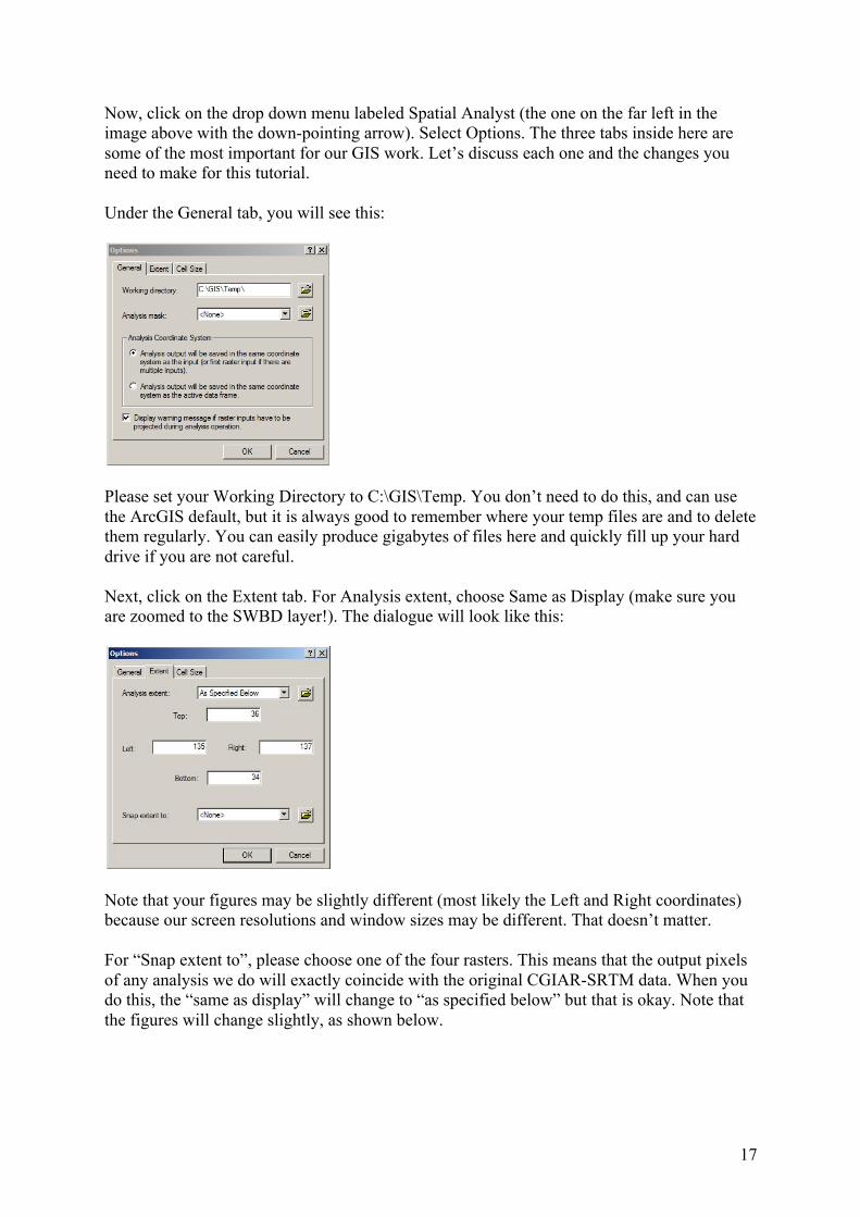
Now, click on the drop down menu labeled Spatial Analyst (the one on the far left in the image above with the down-pointing arrow). Select Options. The three tabs inside here are some of the most important for our GIS work. Let’s discuss each one and the changes you need to make for this tutorial. Under the General tab, you will see this:

Please set your Working Directory to C:\GIS\Temp. You don’t need to do this, and can use the ArcGIS default, but it is always good to remember where your temp files are and to delete them regularly. You can easily produce gigabytes of files here and quickly fill up your hard drive if you are not careful. Next, click on the Extent tab. For Analysis extent, choose Same as Display (make sure you are zoomed to the SWBD layer!). The dialogue will look like this:

Note that your figures may be slightly different (most likely the Left and Right coordinates) because our screen resolutions and window sizes may be different. That doesn’t matter. For “Snap extent to”, please choose one of the four rasters. This means that the output pixels of any analysis we do will exactly coincide with the original CGIAR-SRTM data. When you do this, the “same as display” will change to “as specified below” but that is okay. Note that the figures will change slightly, as shown below.

18

Next, on the Cell Size tab, for Analysis Cell Size, please select any one of the 4 CGIAR-SRTM rasters. You’ll see something like the following:

Select OK. Now we are ready to start doing some calculations with the rasters. In the Spatial Analyst toolbar, open the Raster Calculator. It will look like this:

The Raster Calculator is a great tool. It’s similar to a regular calculator but is able to operate on each individual pixel in a raster. The window on the bottom left (that is currently blank) is the area in which we will perform various calculations on the rasters.

19

Also note that whatever calculations we do here will only be done for the Analysis Extent we set before. Also the output rasters that we make will have a cell size the same as what we set. First, we’d like to merge the four rasters into a single raster, at the same time trimming the extent to something smaller (the “same as display” extent). To do this, enter the following in the Raster Calculator: merge([srtm_63_05.tif],[srtm_63_06.tif],[srtm_64_05.tif],[srtm_64_06.tif]) which appears as:

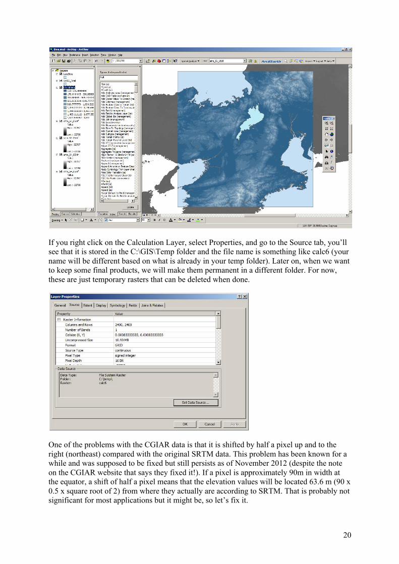
Note that the Raster Calculator is sensitive to context and if you have an extra space or missing comma, etc. the command will return an error. The best policy is to enter as much as possible using the mouse (by clicking the Layers, etc.) and do as little as possible with the keyboard. Click Evaluate. After some processing time, a new raster is added to the map. It looks different but the change in extent may not obvious depending on how you are zoomed in or not. Click on the zoom out icon once to see how the new raster has a smaller extent than the original. Then click the zoom in icon to return to the previous extent. The new raster is shown below. In the Table of Contents, you can see it is called “Calculation” and has a range of values from -38 to 1,892m (again, your values maybe slightly different if the extent is different). Also, if you right click on the Calculation Layer, select Properties, and go to the Source tab, you’ll see that it is stored in the C:\GIS\Temp folder and the file name is something like calc18 (your name will be different based on what is already in your temp folder).

20

If you right click on the Calculation Layer, select Properties, and go to the Source tab, you’ll see that it is stored in the C:\GIS\Temp folder and the file name is something like calc6 (your name will be different based on what is already in your temp folder). Later on, when we want to keep some final products, we will make them permanent in a different folder. For now, these are just temporary rasters that can be deleted when done.

One of the problems with the CGIAR data is that it is shifted by half a pixel up and to the right (northeast) compared with the original SRTM data. This problem has been known for a while and was supposed to be fixed but still persists as of November 2012 (despite the note on the CGIAR website that says they fixed it!). If a pixel is approximately 90m in width at the equator, a shift of half a pixel means that the elevation values will be located 63.6 m (90 x 0.5 x square root of 2) from where they actually are according to SRTM. That is probably not significant for most applications but it might be, so let’s fix it.

21

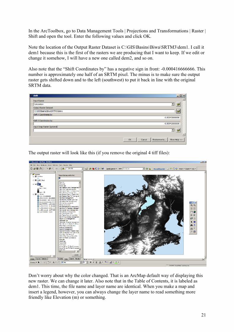
In the ArcToolbox, go to Data Management Tools | Projections and Transformations | Raster | Shift and open the tool. Enter the following values and click OK. Note the location of the Output Raster Dataset is C:\GIS\Basins\Biwa\SRTM3\dem1. I call it dem1 because this is the first of the rasters we are producing that I want to keep. If we edit or change it somehow, I will have a new one called dem2, and so on. Also note that the “Shift Coordinates by” has a negative sign in front: -0.000416666666. This number is approximately one half of an SRTM pixel. The minus is to make sure the output raster gets shifted down and to the left (southwest) to put it back in line with the original SRTM data.

The output raster will look like this (if you remove the original 4 tiff files):

Don’t worry about why the color changed. That is an ArcMap default way of displaying this new raster. We can change it later. Also note that in the Table of Contents, it is labeled as dem1. This time, the file name and layer name are identical. When you make a map and insert a legend, however, you can always change the layer name to read something more friendly like Elevation (m) or something.

22

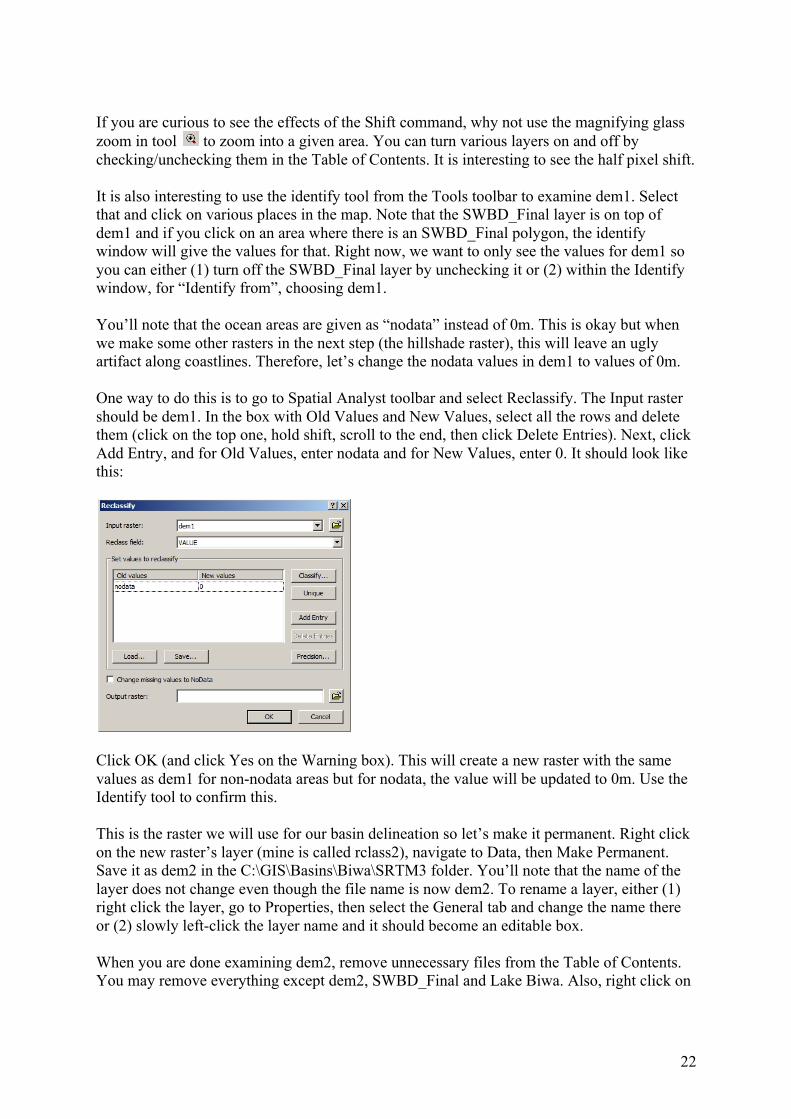
If you are curious to see the effects of the Shift command, why not use the magnifying glass zoom in tool to zoom into a given area. You can turn various layers on and off by checking/unchecking them in the Table of Contents. It is interesting to see the half pixel shift. It is also interesting to use the identify tool from the Tools toolbar to examine dem1. Select that and click on various places in the map. Note that the SWBD_Final layer is on top of dem1 and if you click on an area where there is an SWBD_Final polygon, the identify window will give the values for that. Right now, we want to only see the values for dem1 so you can either (1) turn off the SWBD_Final layer by unchecking it or (2) within the Identify window, for “Identify from”, choosing dem1. You’ll note that the ocean areas are given as “nodata” instead of 0m. This is okay but when we make some other rasters in the next step (the hillshade raster), this will leave an ugly artifact along coastlines. Therefore, let’s change the nodata values in dem1 to values of 0m. One way to do this is to go to Spatial Analyst toolbar and select Reclassify. The Input raster should be dem1. In the box with Old Values and New Values, select all the rows and delete them (click on the top one, hold shift, scroll to the end, then click Delete Entries). Next, click Add Entry, and for Old Values, enter nodata and for New Values, enter 0. It should look like this:

Click OK (and click Yes on the Warning box). This will create a new raster with the same values as dem1 for non-nodata areas but for nodata, the value will be updated to 0m. Use the Identify tool to confirm this. This is the raster we will use for our basin delineation so let’s make it permanent. Right click on the new raster’s layer (mine is called rclass2), navigate to Data, then Make Permanent. Save it as dem2 in the C:\GIS\Basins\Biwa\SRTM3 folder. You’ll note that the name of the layer does not change even though the file name is now dem2. To rename a layer, either (1) right click the layer, go to Properties, then select the General tab and change the name there or (2) slowly left-click the layer name and it should become an editable box. When you are done examining dem2, remove unnecessary files from the Table of Contents. You may remove everything except dem2, SWBD_Final and Lake Biwa. Also, right click on

23

dem2 and select Zoom to Layer. Also, don’t forget to save if you haven’t already been regularly doing that.

Step 8. Changing the Appearance of the elevation data Before beginning the basin delineation, it will be instructive to learn how to make the elevation raster appear more like a professional topographic map. 8.1. Changing the Color Ramp. The colors assigned by default to the elevation data are arbitrary. It sometimes is instructive to use colors that are more representative of what people expect to see in elevations. Open dem2’s Layer Properties and select the Symbology tab. By default, it is probably “Classified” (not “Stretched”) and under “Classification” it will be 9 classes at Equal Intervals. For now, we can just keep these settings. But let’s change the color. Right click on the colored part of the Color Ramp button and uncheck Graphic View. Select “Surface” and click OK. You should see something like this:

The colors here are not necessarily representative of the colors you’d expect in Japan at the given elevations but nevertheless, with that warning in mind, they do somewhat appear closer to what one might expect, i.e. the highest mountains are white, the lowest areas are green. Obviously, in arid areas with no high elevations, this would look silly. Other color ramps would be more appropriate.

24

8.2 Making a Hillshade. One clear way of making the terrain “pop” out to the human eye is to create artificial shadows called a hillshade. Go to the Spatial Analyst toolbar, go to Surface Analysis, then choose Hillshade. Your input should look like this:

The Z factor is set as 0.000011 for this latitude. This is because our data is in a Geographic Coordinate System and requires this correction to make a decent hillshade. Please see the informative article at http://blogs.esri.com/Support/blogs/mappingcenter/archive/2007/06/12/setting-the-z-factor-parameter-correctly.aspx The best way to handle this issue is to make a hillshade while in a Projected Coordinate System but we are not going to discuss that frankly confusing topic yet. Right click on the hillshade raster and make it permanent with the name hshade2 in C:\GIS\Basins\Biwa\SRTM3. Be sure to rename the layer hshade2 (noting you could name it whatever you like but “2” reminds me that the “hshade” comes from dem2). The result should look like this:

At this scale, the hillshade is a little dense. Zoom in a bit, let’s say on the Lake Biwa area. Here you will see the terrain much more clearly as in:

25

8.3 Making a layer semi-transparent. One of the powerful things about GIS software is the ability to drape layers on top of each other and perform analysis based on geographic location. Related to this, we can make one layer semi-transparent so that it “blends” with a layer below it. Let’s do that for the hshade2 so that we can see the dem2 colors a bit. In hshade2’s Layer Properties, go to the Display tab, set Transparency to 50% and click OK. You will now see something like this depending on where you have zoomed to:

26

Delineating the Drainage Basin Once we have the elevation data prepared, we are ready to delineate the drainage basin. This is a 4-step process using the following tools in the Spatial Analyst Toolbox: Fill, Flow Direction, Flow Accumulation, and Watershed. These are discussed in order.

Step 9: The Fill command Making a basin map in ArcGIS requires two things: elevation data and the assumption that water flows downhill. In a natural landscape, including the one described by the SRTM Digital Elevation Model), there are natural depressions which lie lower than the surrounding land. Usually, these are no more than a few meters lower than the surrounding lowest points. Water that enters these depressions may enter the groundwater and drain downhill, it may stagnate and evaporate, or it may fill in with water and pour out. Lake Biwa is an example of the last type: a depression which is filled with water and continuously pouring (“spilling”) out through the Seta River all the way down to Osaka Bay. For our analysis, however, these sort of depressions cannot exist because the ArcGIS program is not able to calculate an exiting flow direction (next step). Therefore, the first step now is to create a DEM without depressions. This is done by the Fill command. (Note: For truly endorheic lake basins---usually containing a salt lake---we need to maintain the depression although I do not discuss the technique here. For the ocean, it doesn’t matter because the flow will always go to the edge of the raster which is a nodata area and “fall off”.) Go to the ArcToolbox and navigate to Spatial Analyst Tools | Hydrology | Fill, and select the tool. Select dem2 as the input raster and name the output as fil2 as per:

This new raster is added to the map but does reveal much information by simple visual inspection. What we would like to see are only the areas that were filled? To do this, go to Raster Calculator and enter the following command:

27

The output raster is called Calculation by default (assuming you deleted the other layers called Calculation from the map!). It does not look very informative with the default display settings. Right click this new layer and Make Permanent as fil2-dem2 (that is a hyphen in between but it looks like a minus sign which makes it easy to remember that we are subtracting dem2 from fil2) in C:\GIS\Basins\Biwa\SRTM3. Also, rename the layer as fil2-dem2. Double click on the layer. Click on Classify, then on Exclusion and exclude values of 0 (we only want to see the areas that were filled…those that were not will be zero because their elevation has not changed). It looks like this:

Click OK. Then, in Classification, choose Quantile, click OK. Then OK again and we get this (turn off the SWBD_Final and LakeBiwa layers to see it better.

28

If you click on the Identify tool , and then use that tool to click on the Lake Biwa area, you’ll get a report like this:

Which shows that Lake Biwa needed to be filled in an incredible 27 m just to pour out to the sea. This is NOT true in reality: the lake naturally drains with no barriers. However, downstream of the lake’s outlet, there is a very narrow valley. The SRTM resolution is approximate 90m and it is not able to fully resolve the outflowing river from the surrounding steep terrain. You can think of the surrounding mountains as influencing the elevation data in the river area. For now, let’s just ignore this (later on, we will “burn” a river into the elevation data to ensure it flows out without Biwa getting filled).

Step 10. The Flow Direction command Assuming for now that fil2 is a “hydrologically-correct” DEM (i.e. there are no depressions remaining), we can use it in the next step which is to calculate the direction of flow from each cell. This will allow us to show the areas where flow accumulates (likely to be rivers) and to show what land is upstream of a given point (the drainage basin).

29

Go to the ArcToolbox, navigate to Spatial Analysis Tools | Hydrology | Flow Direction. Click on it. Select fil2 as the input raster and name the output as dir2 as follows:

The resulting raster looks like this:

This certainly looks strange but it is correct. The direction out of a given cell is assigned one of 8 possible directions represented by the 8 numbers (1,2,4,8,16,32,64,128).

Step 11. The Flow Accumulation Command The next step is to use the Flow Accumulation command. This is not essential for delineating the drainage basin, but is quite helpful, especially if you wish to create a river network (Something we will do later on). The Flow Accumulation tool allows us to determine which cells flow into which cells, i.e. where flow accumulates. Go to the ArcToolbox, navigate to Spatial Analysis Tools | Hydrology | Flow Accumulation. Click on it. Select dir1 as the Input Flow Direction Raster and name the output as acc1 as per:

30

Be sure to set the Output data type to INTEGER and not FLOAT. Turning the SWBD_Final layer back on, and zooming in a bit towards Biwa, the result looks like the following:

This is okay for the downstream as well as for portions of the rivers flowing into Biwa, but it is very wrong for the main part around the lake itself. This is because the lake got filled by 27m in the Fill command. If the lake was indeed 27m higher, rivers would enter the lake where they appear to in the above figure, but this is naturally not the case. After we delineate the basin in the next step, we will remedy this problem.

31

Step 12. The Watershed command Earlier, we made a shapefile called LakeBiwa.shp. We are now going to use that file to determine which land areas flow into Lake Biwa. In other words, we will use the LakeBiwa.shp information as a “pour point”. But to do that, we must first convert the LakeBiwa.shp into a raster. Go to the Spatial Analyst toolbar, select Options. Click the Cell Size tab. Choose Same as Layer “dem2” for the Analysis cell size as per:

Click OK. Then, go to the Extent tab. Choose Same as Layer “dem2” as the Analysis extent (as above). Click OK. Go to the Spatial Analyst toolbar again, choose Feature to Raster from within the Convert item. Choose the following settings:

This will give you a raster with the value of 1 with the same coverage as the Lake_Biwa.shp. (You will get the same result if you choose “ORIG_FID” in the Field option.). Note that you cannot “see” this raster when it is added to the map because ArcMap draws rasters underneath features, by default. If you turn off the SWBD_Final and LakeBiwa shapefile layers, you will see the raster. Now, we are ready to run the Watershed command in the ArcToolbox | Spatial Analysis Tools | Hydrology section. Click Watershed. Execute the command with the following settings:

32

The result looks like this (again, depending on how you zoom in or out):

This is wrong, at least in the sense of Lake Biwa’s real basin, the southern third of which is completely missing. However, considering flaws in the SRTM DEM, this is not surprising.

Step 13. Burning Rivers What we need to do now is edit the SRTM DEM so that the lake pours out naturally through its outflowing river. There are many ways of getting information about the location of the actual outlet but one simple method is to go to Google Earth and tract a path from the exit area of the lake, downstream far enough to get past the bottleneck point. Open Google Earth. Click on the “Add Path” tool as follows:

33

Trace the river down as far as it takes to get to a flat urban area. After a bit of practice, you will get good at zooming in and out and panning around the scene to achieve the best settings for tracing the river on screen. Click OK in the dialog box. Then, in the Layers bar on the lefthand side in Google Earth, right click the file you just made and choose “Save Place As” Biwa_out1.kml in C:GIS\Basins\Biwa\SRTM3 In ArcGIS, click the Add Data icon ( ) and select this file. ArcGIS9.3 can import KML files but it tends to bring in a lot of extraneous layers as per:

Delete all of those except Placemark Line (later on, if you use the Add Polygon tool in Google Earth to trace a polygon like a lake, you will want to keep “Placemark Polygon”

34

instead). Then, right click on Placemark Line, choose Data, then Export Data and save it as Biwa_out1.shp:

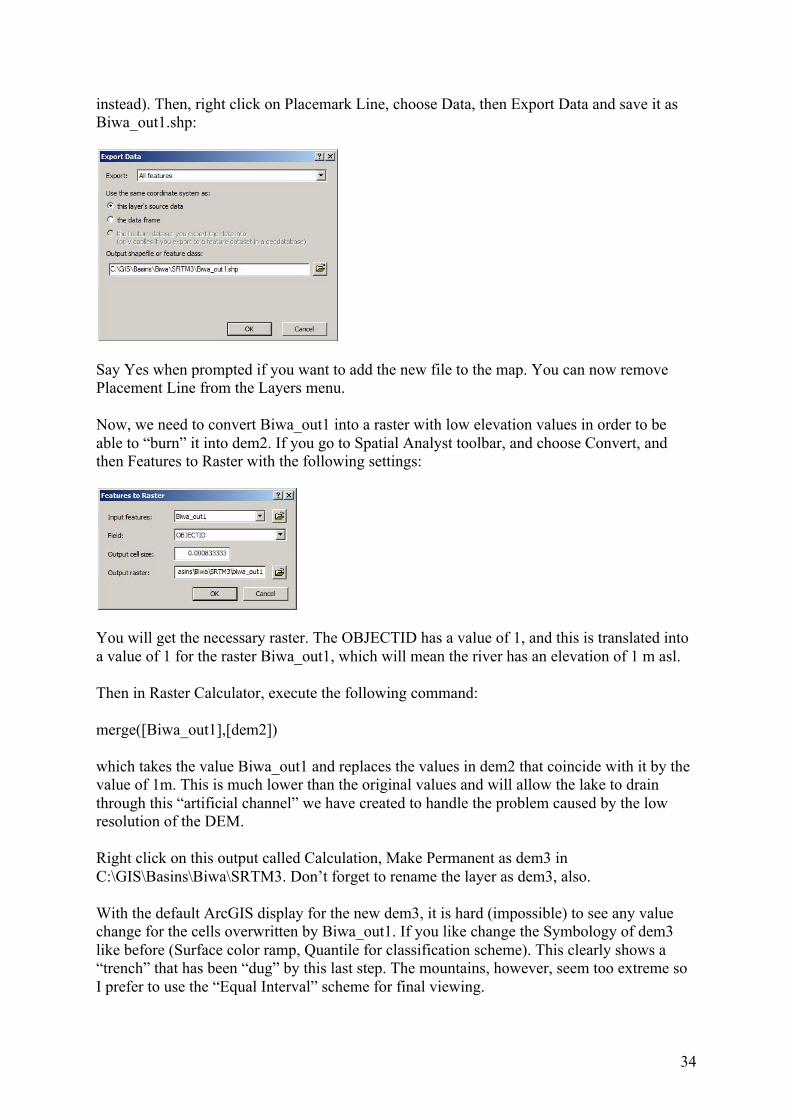
Say Yes when prompted if you want to add the new file to the map. You can now remove Placement Line from the Layers menu. Now, we need to convert Biwa_out1 into a raster with low elevation values in order to be able to “burn” it into dem2. If you go to Spatial Analyst toolbar, and choose Convert, and then Features to Raster with the following settings:

You will get the necessary raster. The OBJECTID has a value of 1, and this is translated into a value of 1 for the raster Biwa_out1, which will mean the river has an elevation of 1 m asl. Then in Raster Calculator, execute the following command: merge([Biwa_out1],[dem2]) which takes the value Biwa_out1 and replaces the values in dem2 that coincide with it by the value of 1m. This is much lower than the original values and will allow the lake to drain through this “artificial channel” we have created to handle the problem caused by the low resolution of the DEM. Right click on this output called Calculation, Make Permanent as dem3 in C:\GIS\Basins\Biwa\SRTM3. Don’t forget to rename the layer as dem3, also. With the default ArcGIS display for the new dem3, it is hard (impossible) to see any value change for the cells overwritten by Biwa_out1. If you like change the Symbology of dem3 like before (Surface color ramp, Quantile for classification scheme). This clearly shows a “trench” that has been “dug” by this last step. The mountains, however, seem too extreme so I prefer to use the “Equal Interval” scheme for final viewing.

35

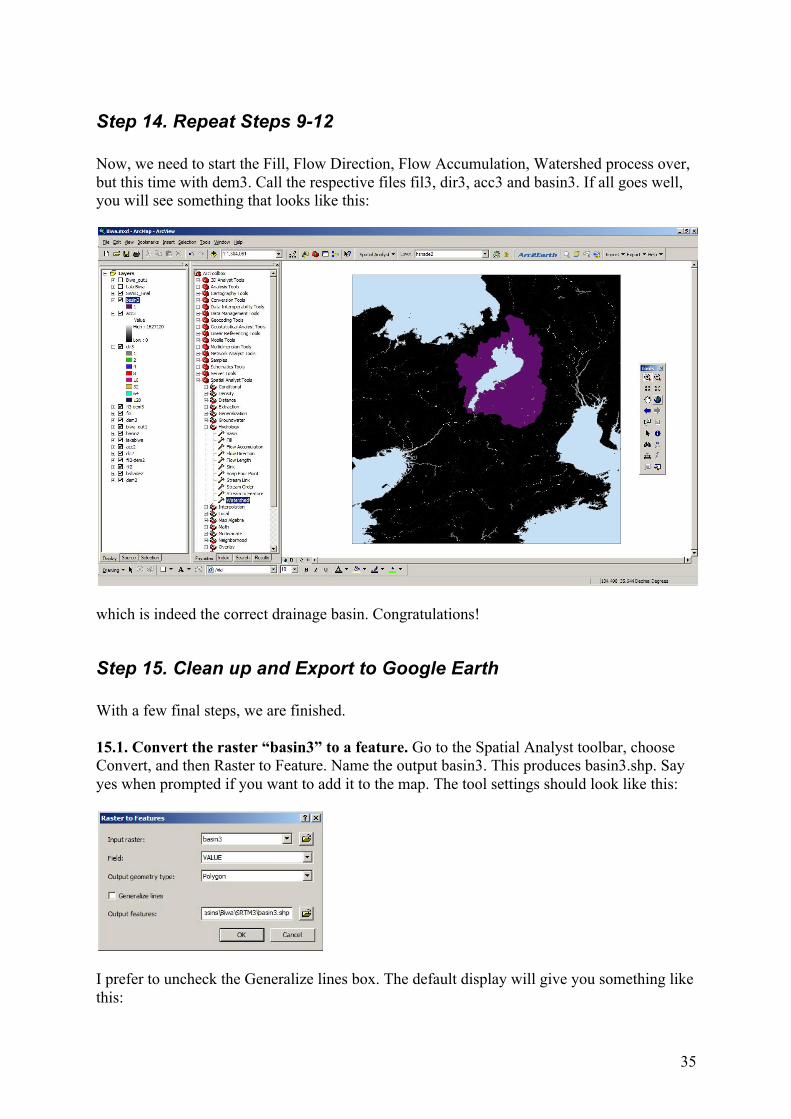
Step 14. Repeat Steps 9-12 Now, we need to start the Fill, Flow Direction, Flow Accumulation, Watershed process over, but this time with dem3. Call the respective files fil3, dir3, acc3 and basin3. If all goes well, you will see something that looks like this:

which is indeed the correct drainage basin. Congratulations!

Step 15. Clean up and Export to Google Earth With a few final steps, we are finished. 15.1. Convert the raster “basin3” to a feature. Go to the Spatial Analyst toolbar, choose Convert, and then Raster to Feature. Name the output basin3. This produces basin3.shp. Say yes when prompted if you want to add it to the map. The tool settings should look like this:

I prefer to uncheck the Generalize lines box. The default display will give you something like this:

36

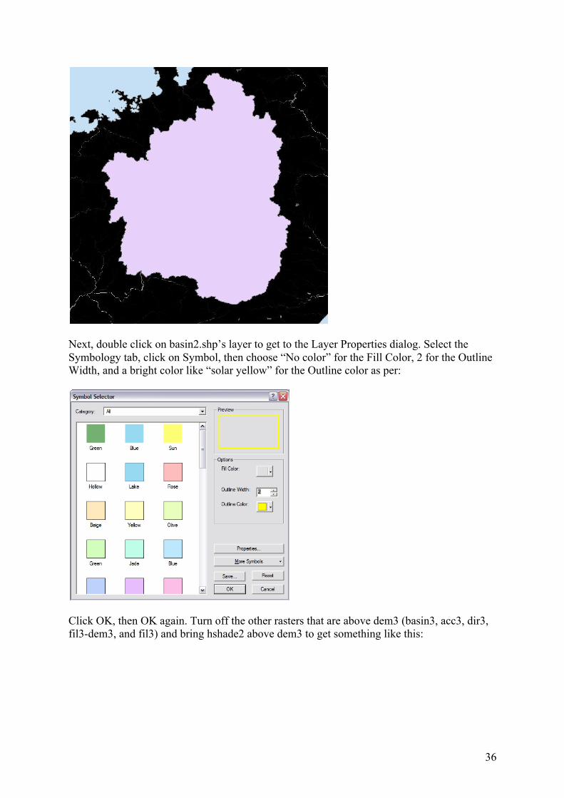
Next, double click on basin2.shp’s layer to get to the Layer Properties dialog. Select the Symbology tab, click on Symbol, then choose “No color” for the Fill Color, 2 for the Outline Width, and a bright color like “solar yellow” for the Outline color as per:

Click OK, then OK again. Turn off the other rasters that are above dem3 (basin3, acc3, dir3, fil3-dem3, and fil3) and bring hshade2 above dem3 to get something like this:

37

15.2 Export to Google Earth. Next, if you like, you can export the basin2.shp to Google Earth to see how it looks on top of satellite images (In the tutorial on “Classifying Land Cover”, we discuss how to do this in GIS with a Landsat image). Go to ArcToolbox | Conversion Tools | To KML | Layer to KML and execute the tool with the following settings:

Note that if you try to save the file as basin3 inside the SRTM3 folder, there is a bug in the current 9.3 version that redirects you to the folder SRTM3\basin2. I just add “GE” to the file name to avoid this issue. Open Google Earth, and from the main menu, select Open and navigate to the basin3_GE.kmz file. You should see something like this, with the basin outline in yellow:

38

15.3 Clean up. Finally, you should clean up the map by removing unnecessary layers. After 6 hours or so of work (typical time it takes to do this task for a beginner), you will end up with something like this:

Good job!

39

Further Work As you can imagine, there are many other tasks you could perform:

• For one, you’d like to calculate the area of the Lake Biwa basin and perhaps the area of lake itself.

• You’d probably like to add some other layers such as Population and calculate the population of the drainage basin.

• You could add political boundaries and calculate what percentage of the basin is in each jurisdiction.

• Using the Flow Accumulation raster, you could make a River Network. • You could add existing Land Use/Land Cover data or add a Landsat image and

classify it yourself. • You could design a professional looking map with scale bars, legends, etc. • And so on…

As you’ve seen, GIS can be challenging to use but patience and effort has its rewards. You now have the power to do your own drainage basin delineation: the key first step in using geospatial technologies for lake basin management! Please contact me if you need any assistance in your future work or questions about this tutorial.