deliverable d3.2 channel and ... - ict-terranova.eu€¦ · terranova project page 2 of 63...
TRANSCRIPT
D3.2 – Channel and Propagation Modelling and Characterization
TERRANOVA Project Page 1 of 63
This project has received funding from Horizon 2020, European Union’s
Framework Programme for Research and Innovation, under grant agreement
No. 761794
Deliverable D3.2 Channel and Propagation Modelling
and Characterization Work Package 3 - THz Wireless Link Design
TERRANOVA Project
Grant Agreement No. 761794
Call: H2020-ICT-2016-2
Topic: ICT-09-2017 - Networking research beyond 5G
Start date of the project: 1 July 2017
Duration of the project: 30 months

D3.2 – Channel and Propagation Modelling and Characterization
TERRANOVA Project Page 2 of 63
Disclaimer This document contains material, which is the copyright of certain TERRANOVA contractors, and
may not be reproduced or copied without permission. All TERRANOVA consortium partners
have agreed to the full publication of this document. The commercial use of any information
contained in this document may require a license from the proprietor of that information. The
reproduction of this document or of parts of it requires an agreement with the proprietor of
that information. The document must be referenced if used in a publication.
The TERRANOVA consortium consists of the following partners.
No. Name Short Name Country
1
(Coordinator)
University of Piraeus Research Center UPRC Greece
2 Fraunhofer Gesellschaft (FhG-HHI & FhG-IAF) FhG Germany
3 Intracom Telecom ICOM Greece
4 University of Oulu UOULU Finland
5 JCP-Connect JCP-C France
6 Altice Labs ALB Portugal
7 PICAdvanced PIC Portugal

D3.2 – Channel and Propagation Modelling and Characterization
TERRANOVA Project Page 3 of 63
Document Information
Project short name and number TERRANOVA (761794)
Work package WP3
Number D3.2
Title Channel and propagation modelling and
characterization
Version V1.0
Responsible unit UOULU
Involved units UOULU, UPRC, ICOM
Type1 R
Dissemination level2 PU
Contractual date of delivery 31.08.2018
Last update 31.08.2018
1 Types. R: Document, report (excluding the periodic and final reports); DEM: Demonstrator, pilot,
prototype, plan designs; DEC: Websites, patents filing, press & media actions, videos, etc.; OTHER:
Software, technical diagram, etc. 2 Dissemination levels. PU: Public, fully open, e.g. web; CO: Confidential, restricted under conditions set
out in Model Grant Agreement; CI: Classified, information as referred to in Commission Decision
2001/844/EC.

D3.2 – Channel and Propagation Modelling and Characterization
TERRANOVA Project Page 4 of 63
Document History
Version Date Status Authors, Reviewers Description
v0.01 08.08.2018 Draft Joonas Kokkoniemi
(UOULU)
Initial version (v0.01)
v0.02 20.08.2018 Draft Alexandros-Apostolos A.
Boulogeorgos (UPRC)
Corrections to the previous
version.
v0.03 22.08.2018 Draft Janne Lehtomäki
(UOULU)
Raytracing simulation model.
v0.04 23.08.2018 Draft Alexandros-Apostolos A.
Boulogeorgos (UPRC)
Fading literature review.
v0.05 24.08.2018 Draft Joonas Kokkoniemi
(UOULU)
Corrections to the previous
version and Geometrical
simulation model.
v0.06 29.08.2018 Draft Georgia Ntouni (ICOM) Corrections to the previous
version.
v1.0 31.08.2018 Final Markku Juntti (UOULU)
Janne Lehtomäki
(UOULU)
Joonas Kokkoniemi
(UOULU)
Angeliki Alexiou (UPRC)
Final Editorial Corrections
D3.2 – Channel and Propagation Modelling and Characterization
TERRANOVA Project Page 5 of 63
Acronyms and Abbreviations
Acronym/Abbreviation Description
BEP Bit error probability
BPSK Binary phase shift keying
EM Electromagnetic
FSPL Free space path loss
GEO Geostationary orbit
GPU Graphics processing unit
HITRAN High-resolution transmission molecular
absorption database
LEO Low Earth orbit
LOS Line-of-sight
MAC Medium access control
MDF Medium density fibreboard
NLOS Non-line-of-sight
PHY Physical layer
QAM Quadrature amplitude modulation
Rx Receiver
SINR Signal-to-interference-plus-noise ratio
SNR Signal-to-noise ratio
Tx Transmitter
UTD Uniform theory of diffraction

D3.2 – Channel and Propagation Modelling and Characterization
TERRANOVA Project Page 6 of 63
Contents
1. Introduction ............................................................................................................................... 11
2. THz band LOS channels ............................................................................................................ 12
2.1 Molecular absorption ..................................................................................................... 12
2.2 Path loss ......................................................................................................................... 12
2.3 Numerical results for the LOS paths ............................................................................. 13
2.4 Rain and fog attenuation ................................................................................................ 20
3. Generalized channel model ....................................................................................................... 22
4. Simplified channel models for 200 – 450 GHz band ................................................................ 32
4.1 Model for 200 – 400 GHz band ..................................................................................... 32
4.2 Model for 200 – 450 GHz band ..................................................................................... 35
5. Transmission windows below one terahertz .............................................................................. 38
5.1 Transmission windows in the 0.275 – 1 THz band ....................................................... 38
5.2 Simplified estimate for 200 – 400 GHz band ................................................................ 41
6. The channel measurements ........................................................................................................ 44
6.1 The Measurement setup ................................................................................................. 44
6.2 Theoretical reflection loss ............................................................................................. 46
6.3 Theoretical scattering loss ............................................................................................. 48
7. Noise in the THz band ............................................................................................................... 50
8. Fading in THz band ................................................................................................................... 52
9. Simulation for studying fading, interference, and multipath propagation ................................. 53
9.1 Ray-tracing approach..................................................................................................... 53
9.2 Geometric simulation model ......................................................................................... 56
10. Future work ............................................................................................................................. 59
11. Conclusions ............................................................................................................................. 60
References ..................................................................................................................................... 61

D3.2 – Channel and Propagation Modelling and Characterization
TERRANOVA Project Page 7 of 63
List of Figures
Fig. 1. Molecular absorption loss in the THz band. ...................................................................... 14 Fig. 2. Molecular absorption loss around the 300 GHz band. ....................................................... 14 Fig. 3. Losses as a function of frequency per 1 km link distance. ................................................. 15 Fig. 4. Total path loss in the THz band as a function of distance and frequency up to 100 meters.
....................................................................................................................................................... 16 Fig. 5. Total path loss around the 300 GHz as a function of distance and frequency up to 1 km. 16 Fig. 6. The distance after which the molecular absorption loss becomes the dominant loss
mechanism. .................................................................................................................................... 18 Fig. 7. The distance after which the molecular absorption loss becomes the dominant loss
mechanism around the 300 GHz band. .......................................................................................... 19 Fig. 8. Comparison of the molecular absorption loss and free space path loss as a function of the
distance and the frequency up to 10 km distance. ......................................................................... 19 Fig. 9. Comparison of the molecular absorption loss and free space path loss as a function of the
distance and the frequency up to 1 km distance. ........................................................................... 20 Fig. 10. Rain attenuation (dB/km) as a function of frequency for different precipitation levels... 21 Fig. 11. One possible terrestrial scenario for the generalized channel model. .............................. 22 Fig. 12. A path through the atmosphere where the plane parallel assumption fall short on properly
explaining the structure of the atmosphere (picture of the Earth from Nasa: NASA/NOAA/GOES
Project). ......................................................................................................................................... 24 Fig. 13. Geometry of a general path through the atmosphere (picture of the Earth from Nasa:
NASA/NOAA/GOES Project)......................................................................................................... 25 Fig. 14. Predicted distance through the atmosphere for the plane parallel approximation and for
the proposed model. ...................................................................................................................... 26 Fig. 15. Average water vapor mixing ratio and distribution on global scale, and the mean altitude
(m) of the corresponding value on the left-hand figure. ................................................................ 26 Fig. 16. Mean pressure and temperature of the atmosphere as a function of altitude (data from
1976 US Standard atmosphere [11]). ............................................................................................ 27 Fig. 17. Per-kilometer losses for different altitudes. ..................................................................... 29 Fig. 19. Path loss as a function of altitude and frequency for a 100 meter link. ........................... 30 Fig. 20. Path loss from ground to air as a function of frequency. ................................................. 31 Fig. 21. SNR bounds for BPSK and 64-QAM for BEP= . .................................................. 31
Fig. 22. Performance of the proposed simplified molecular absorption loss model. .................... 33 Fig. 23. Performance of the proposed simplified molecular absorption loss model compared to
other models. ................................................................................................................................. 34 Fig. 24. Close-up of Fig. 23 at 300 – 400 GHz band..................................................................... 35 Fig. 25. Absorption loss according to the extended simplified model detailed above. ................. 37 Fig. 26. Close up of Fig. 25 to better illustrate the error made in the absorption loss estimate by
the simplified model versus the fully accurate model. .................................................................. 37 Fig. 27. Path loss and transmission windows at 10 meter. ............................................................ 39 Fig. 28. Path loss and transmission windows at 100 meter. .......................................................... 39 Fig. 29. Available bandwidths at 10 meter. ................................................................................... 40 Fig. 30. Available bandwidths at 100 meter. ................................................................................. 40

D3.2 – Channel and Propagation Modelling and Characterization
TERRANOVA Project Page 8 of 63
Fig. 31. The predicted available bandwidths for three different distances and two different relative
humidity values at the transmission centre frequency 342 GHz. .................................................. 42 Fig. 32. Available bandwidth progression for two different relative humidity values at the
transmission centre frequency 342 GHz. ....................................................................................... 42 Fig. 33. Minimum bandwidth as a function of frequency and relative humidity at the transmission
centre frequency 342 GHz. ............................................................................................................ 43 Fig. 34. Maximum bandwidth as a function of frequency and relative humidity at the transmission
centre frequency 342 GHz. ............................................................................................................ 43 Fig. 35: TeraView TeraPulse measurement setup. ........................................................................ 45 Fig. 36: Measured materials. ......................................................................................................... 45 Fig. 37: Measured and fitted reflection loss for laminated medium density fibreboard (MDF) at
300 GHz. Red line represents an equivalent reflection loss for circularly polarized light with the
given refractive index. ................................................................................................................... 47 Fig. 38: Measured and theoretical scattering and reflection loss for plaster at 300 GHz at 45
degree incidence angle. ................................................................................................................. 49 Fig 39. Antenna brightness temperature as a function of frequency. ............................................ 51 Fig. 40. Flow of data in ray tracing calculations. .......................................................................... 53 Fig. 41. Office room (adapted from [30]) with four transmitters (in the corners close to roof) and
35 possible locations for a receiver. Different colours indicate different materials (concrete, glass,
painted wood, rubber floor, laminated MDF)................................................................................ 54 Fig. 42. Scatter points in the office room. ..................................................................................... 55 Fig. 43. Delay spread as a function of beam angle for receivers 1, 15, and 30. Center frequency is
equal to 300 GHz. .......................................................................................................................... 55 Fig. 44. An illustration of the simulation model with the desired and other users, and reflected and
random paths. ................................................................................................................................ 57
Fig. 45. Simulated average SINR and SINR thresholds for 16-QAM and BPSK for BEP.
....................................................................................................................................................... 57 Fig. 46. Simulated signal and interference powers and the noise power. ...................................... 58

D3.2 – Channel and Propagation Modelling and Characterization
TERRANOVA Project Page 9 of 63
List of Tables
Table 1. Tabled values for the LOS losses per 1 km link from 100 GHz to 880 GHz. ................. 17 Table 2: Fitted refractive indices to the measured reflection losses. ............................................. 47 Table 3: Parameters for the scattering loss of the measured materials. ......................................... 48

D3.2 – Channel and Propagation Modelling and Characterization
TERRANOVA Project Page 10 of 63
Executive Summary
This Deliverable, D3.2 – Channel and propagation modelling and characterization, focuses on the
channel modelling for the THz links. The knowledge of the channels is very important when
considering application and use case –specific communication solutions and most importantly,
when considering link budgets and theoretical capacities. The work consists of theoretical
channel models for arbitrary length line-of-sight (LOS) links, as well as measurement-based non-
line-of-sight (NLOS) link modelling. The derived models cover the needs of the TERRANOVA
communication scenarios. Based on the derived models, the TERRANOVA scenarios defined in
WP1 can be tested and analysed. The derived models are also useful beyond TERRANOVA in
generic THz research on arbitrary scale communication systems.

D3.2 – Channel and Propagation Modelling and Characterization
TERRANOVA Project Page 11 of 63
1. INTRODUCTION
The terahertz band (0.1 – 10 THz) communications systems have been under dense research
during the past few years. The obvious reasons are the vast frequency resources making it
possible to achieve very high data rates and/or enhance the spectrum sharing opportunities
among large numbers of users and devices. Due to challenges in implementation of the THz
capable transceivers, the utilization of the full THz band is demanding. A first step is to conquer
the below 1 THz frequencies, which is one of the fundamental objectives of the TERRANOVA
project.
Regardless of the application or the use-case of any frequency band, the knowledge of the
channel(s) is in focal point for understanding the signal behaviour in the medium. By proper
channel knowledge, an investigation of the potential communication solutions becomes
possible. Each frequency band has its own peculiarities and fading characteristics that have an
impact on the utilizable bandwidths, modulations, coding, etc. For this reason, great effort has
been put to studying and modelling the different THz bands. Intense channel investigation is
particularly important in these relatively poorly explored frequencies. Most of the existing
channel models focus on Beer-Lambert’s law with fixed absorption coefficient. This is a good
baseline model and also the starting point of the channel research for TERRANOVA. New
channel models are required because the TERRANOVA use cases vary from TERRANOVA
backhaul, i.e., a long distance (~1 km) backhaul for base station-to-base station links, to short
indoor communication links with other users and non-line-of-sight (NLOS) links. Off the shelf
models for all the TERRANOVA use cases do not exist, and thus, the channel modelling herein is
utilized to extend existing models and derive new ones to realistically model the propagation
environments.
In order to address the signal propagation in the various TERRANOVA scenarios and use cases,
the work in T3.1 of WP3 has been focusing on modelling the channel propagation characteristics
in various scales of communication. The main focus is on the below 1 THz frequency bands, but
since the channel models derived herein are valid over the entire THz band, some results are
given on the full 0.1 to 10 THz band. This document, Deliverable D3.2, describes the derived
channel models. Those include theoretical line-of-sight (LOS) models as well as NLOS modelling
via measurements. All the models herein are derived in a generic way, so that they can be
utilized and scaled based on the application, or use case in hand. The presented models have
been utilized in few publications during the TERRANOVA project [1] [2] [3] [4].
The work in this document is organized as follows. First the background on LOS channel
modelling is introduced, after which, the general and simplified LOS channel models are
reported. The measurements on NLOS paths are gone through next, followed by a short
discussion on the noise processes in the THz band. Finally, we discuss about fading on the THz
frequencies as well as simulation models utilized to study multipath and multiuser propagation
and fading.

D3.2 – Channel and Propagation Modelling and Characterization
TERRANOVA Project Page 12 of 63
2. THZ BAND LOS CHANNELS
The THz band signals experience fading even in the full LOS path because of the discrete
molecular absorption loss. The free space path loss, on the other hand, is always present due to
natural expansion of the electromagnetic waves in the medium. These phenomena are briefly
looked in this section serving as a background for most of the research done for TERRANOVA.
2.1 Molecular absorption
Molecular absorption is usually modelled by transmittance, i.e., the fraction of the energy
capable of propagating through the channel. It is calculated by Beer-Lambert’s law [5] [6] as
where is the frequency, is the distance from transmitter (Tx) to receiver (Rx), and
are transmitted and received power, respectively, is the absorption coefficient of
th absorbing species (molecule or its isotopologue) at frequency , and is the angle of
incident wave (not valid in homogenous spherically symmetric space). The absorption
coefficient is defined as
where is the number density of the molecules and is the absorption cross section of a
single molecule. The latter term is further defined by spectral line intensity and line shape
as
and thus, the molecular absorption coefficient depends on temperature , pressure , and
molecular composition of the channel. Further details on the absorption coefficient can be
found in the references herein and in the upcoming sections of this document, where the
detailed derivations of various propagation models are given.
2.2 Path loss
If we only consider LOS channel, molecular absorption loss and free space path loss (FSPL) are
the main loss mechanisms. Increased loss may be introduced by rain or fog discussed later, and

D3.2 – Channel and Propagation Modelling and Characterization
TERRANOVA Project Page 13 of 63
possibly scattering on impurities of the air [7]. However, in the general case we only have the
FSPL and the molecular absorption loss. The FSPL is defined as
where and are Rx and Tx antenna gains, and is the speed of light. The molecular
absorption loss is given as an inverse of (1). Therefore, the LOS path loss becomes (path gain in
the below form)
The numerical examples for the total loss below were calculated by using this expression, or its
inverse for path loss figures and are shown in the next section.
2.3 Numerical results for the LOS paths
Some numerical results for the molecular absorption loss and the FSPL are given below. Most of
them are calculated assuming isotropic antennas unless otherwise stated. As a consequence,
path losses are relatively high for long distance links. Molecular absorption loss values are
calculated at 296 K temperature, 101325 Pa pressure, and 50% relative humidity.
Fig. 1 shows the molecular absorption loss for the full THz band for one and five meter
distances. This figure shows the biggest problem in the higher THz band on long distance links: if
signals are not killed by the free space loss, then they are killed by the molecular absorption
loss, or the combination of both. Therefore, the full THz band is mainly useful for very short
distance links. It should be noticed that transmittance is usually given in linear scale (like below).
Thus, the total losses in Fig. 1 are not as severe as they appear. Regardless of this, the molecular
absorption loss increases exponentially and becomes an intense problem as the link distance
increases. This will be better shown below when free space loss is compared to the molecular
absorption loss.
Fig. 2 shows the transmittance for the 300 GHz region considering a variety of distances from 1
m to 2 km. It becomes obvious that the losses are considerably lower in the lower THz band, but
at the same time there are some deeply faded frequencies. Still, the distances are already very
reasonable for long distance communications compared with the full THz band. In particular,
frequencies around 300 GHz are modestly attenuated and most of the attenuation will come
from other sources, such the free space path loss.

D3.2 – Channel and Propagation Modelling and Characterization
TERRANOVA Project Page 14 of 63
Fig. 1. Molecular absorption loss in the THz band.
Fig. 2. Molecular absorption loss around the 300 GHz band.
D3.2 – Channel and Propagation Modelling and Characterization
TERRANOVA Project Page 15 of 63
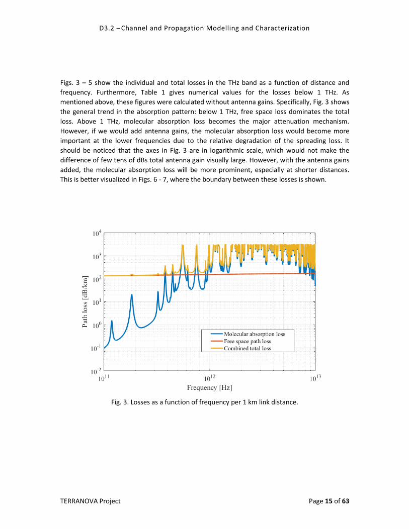
Figs. 3 – 5 show the individual and total losses in the THz band as a function of distance and
frequency. Furthermore, Table 1 gives numerical values for the losses below 1 THz. As
mentioned above, these figures were calculated without antenna gains. Specifically, Fig. 3 shows
the general trend in the absorption pattern: below 1 THz, free space loss dominates the total
loss. Above 1 THz, molecular absorption loss becomes the major attenuation mechanism.
However, if we would add antenna gains, the molecular absorption loss would become more
important at the lower frequencies due to the relative degradation of the spreading loss. It
should be noticed that the axes in Fig. 3 are in logarithmic scale, which would not make the
difference of few tens of dBs total antenna gain visually large. However, with the antenna gains
added, the molecular absorption loss will be more prominent, especially at shorter distances.
This is better visualized in Figs. 6 - 7, where the boundary between these losses is shown.
Fig. 3. Losses as a function of frequency per 1 km link distance.

D3.2 – Channel and Propagation Modelling and Characterization
TERRANOVA Project Page 16 of 63
Fig. 4. Total path loss in the THz band as a function of distance and frequency up to 100 meters.
Fig. 5. Total path loss around the 300 GHz as a function of distance and frequency up to 1 km.

D3.2 – Channel and Propagation Modelling and Characterization
TERRANOVA Project Page 17 of 63
Table 1. Tabled values for the LOS losses per 1 km link from 100 GHz to 880 GHz.
Frequency (GHz)
100 120 140 160 180 200 220 240 260 280
Absorption loss (dB)
0.1 1.1 0.2 0.5 9.8 1.3 0.8 0.8 1.0 1.2
Free space loss (dB)
132.4 134.0 135.4 136.5 137.6 138.5 139.3 140.1 140.7 141.4
Total loss (dB)
132.5 135.1 135.6 137.0 147.3 139.8 140.0 140.8 141.7 142.6
Frequency (GHz)
300 320 340 360 380 400 420 440 460 480
Absorption loss (dB)
1.8 9.1 4.2 7.6 231.0 11.2 10.5 65.5 29.1 31.5
Free space loss (dB)
142.0 142.6 143.1 143.6 144.0 144.5 144.9 145.3 145.7 146.1
Total loss (dB)
143.8 151.7 147.3 151.1 375.0 155.7 155.4 210.8 174.8 177.6
Frequency (GHz)
500 520 540 560 580 600 620 640 660 680
Absorption loss (dB)
41.1 95.5 444.6 N/A /INF
313.9 102.1 230.2 41.5 39.9 35.0
Free space loss (dB)
146.4 146.8 147.1 147.4 147.7 148.0 148.3 148.6 148.8 149.1
Total loss (dB)
187.5 242.3 591.7 N/A /INF
461.7 250.1 378.5 190.1 188.7 184.0
Frequency (GHz)
700 720 740 760 780 800 820 840 860 880
Absorption loss (dB)
47.4 98.7 595.2 1450 147.6 63.5 42.0 35.6 38.4 36.3
Free space loss (dB)
149.3 149.6 149.8 150.1 150.3 150.5 150.7 150.9 151.1 151.3
Total loss (dB)
196.8 248.3 745.0 1600 297.9 214 192.7 186.5 189.5 187.6

D3.2 – Channel and Propagation Modelling and Characterization
TERRANOVA Project Page 18 of 63
Figs. 6 and 7 show the boundary distance after which the molecular absorption becomes the
dominant loss, or putting it the other way, below which the free space loss is the dominant loss
mechanism. The antenna gain herein refers to the total combined gain, i.e. from Rx and Tx.
Furthermore, the maximum distance was set equal to 10 km because the molecular absorption
gain tends towards zero, as the distance tends to infinity. It is obvious that at frequencies above
1 THz the molecular absorption loss takes over quite fast, only after few meters to some tens of
meters, in general. Especially, in Fig. 7, we can observe that the molecular absorption becomes
the dominant loss at lower distance as the antenna gains increase. This is simply because the
molecular absorption loss only depends on distance and not on the angles.
Figs. 8 and 9 give some further comparisons of the molecular absorption loss to the FSPL around
the 300 GHz frequency band and up to 1 and 10 km, respectively. Indeed, in this band, the free
space loss is the most important loss, but depending on the target frequencies and bandwidths,
and ultimately, the target distances as seen in Figs. 6 and 7. In some bands, the FSPL is enough
to predict the total loss, whereas in other bands, or over very wide bandwidths, the molecular
absorption needs to be taken into account.
Fig. 6. The distance after which the molecular absorption loss becomes the dominant loss mechanism.

D3.2 – Channel and Propagation Modelling and Characterization
TERRANOVA Project Page 19 of 63
Fig. 7. The distance after which the molecular absorption loss becomes the dominant loss mechanism around the 300 GHz band.
Fig. 8. Comparison of the molecular absorption loss and free space path loss as a function of the distance and the frequency up to 10 km distance.

D3.2 – Channel and Propagation Modelling and Characterization
TERRANOVA Project Page 20 of 63
Fig. 9. Comparison of the molecular absorption loss and free space path loss as a function of the distance and the frequency up to 1 km distance.
2.4 Rain and fog attenuation
Other aspects of the outdoor propagation that should be considered are the rain and fog/mist
attenuations. These may become an issue in cases where long distance backhaul links are
studied. The rain attenuations for various precipitation rates are given in Fig. 10 in dB/km. The
attenuation curves in Fig. 10 are based on the ITU-R report P.838-3 [8]. Those are calculated for
a circular polarization, although, the vertical and the horizontal polarizations have nearly
identical attenuation curves as a function of frequency. More information on exact calculation
of the rain attenuation can be found in [8].
We can see that the rain attenuations for different precipitation levels below 1 THz frequencies
are rather modest. This is the case especially in northern countries. For instance, in Oulu,
Finland, average rainfall during the summer months is roughly speaking between 50 – 100 mm
per month. Of course, the situation changes quite a lot when moving south, where heavier rains
are more common. Furthermore, instantaneous rainfall can be very high, even if the monthly
means are low.
ITU-R also gives attenuation models for fog and clouds up to 1 THz frequency [9]. However, it
should be noted that both the fog and the rain attenuation models have some uncertainty. For
instance, in ITU-R recommendation P.838-2, they mention that the attenuation numbers are
tested and accurate up to 55 GHz. In P.838-3, this clause is missing and that particular document
does not justify the models very accurately. Regardless of this uncertainty, these models can be
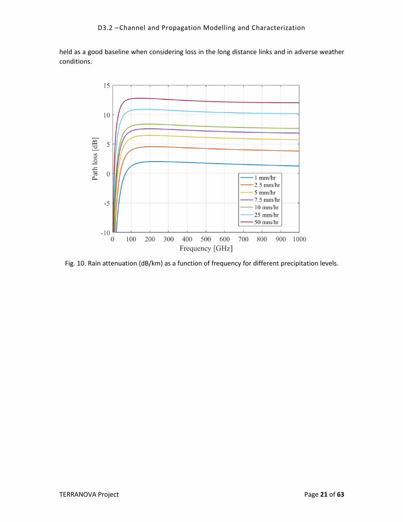
D3.2 – Channel and Propagation Modelling and Characterization
TERRANOVA Project Page 21 of 63
held as a good baseline when considering loss in the long distance links and in adverse weather
conditions.
Fig. 10. Rain attenuation (dB/km) as a function of frequency for different precipitation levels.
D3.2 – Channel and Propagation Modelling and Characterization
TERRANOVA Project Page 22 of 63
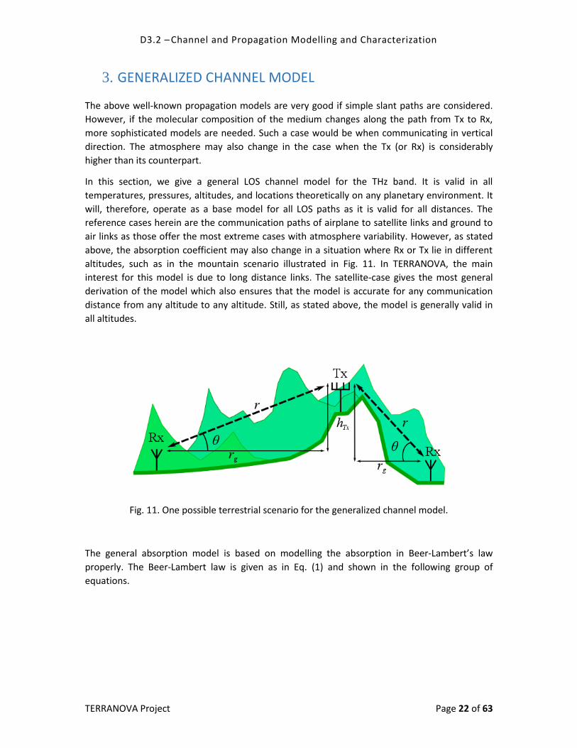
3. GENERALIZED CHANNEL MODEL
The above well-known propagation models are very good if simple slant paths are considered.
However, if the molecular composition of the medium changes along the path from Tx to Rx,
more sophisticated models are needed. Such a case would be when communicating in vertical
direction. The atmosphere may also change in the case when the Tx (or Rx) is considerably
higher than its counterpart.
In this section, we give a general LOS channel model for the THz band. It is valid in all
temperatures, pressures, altitudes, and locations theoretically on any planetary environment. It
will, therefore, operate as a base model for all LOS paths as it is valid for all distances. The
reference cases herein are the communication paths of airplane to satellite links and ground to
air links as those offer the most extreme cases with atmosphere variability. However, as stated
above, the absorption coefficient may also change in a situation where Rx or Tx lie in different
altitudes, such as in the mountain scenario illustrated in Fig. 11. In TERRANOVA, the main
interest for this model is due to long distance links. The satellite-case gives the most general
derivation of the model which also ensures that the model is accurate for any communication
distance from any altitude to any altitude. Still, as stated above, the model is generally valid in
all altitudes.
Fig. 11. One possible terrestrial scenario for the generalized channel model.
The general absorption model is based on modelling the absorption in Beer-Lambert’s law
properly. The Beer-Lambert law is given as in Eq. (1) and shown in the following group of
equations.
D3.2 – Channel and Propagation Modelling and Characterization
TERRANOVA Project Page 23 of 63
The absorption coefficient depends on various parameters, such as pressure , temperature ,
molecular composition of the channel, line intensity , and line shape . Transmittance in plane
parallel atmosphere, i.e., assuming planar atmosphere with distance dependent absorption
coefficient (between points and ), is simply given by
The plane parallel atmosphere is a very good approximation up to certain limits, e.g., when
considering perfectly vertical paths, or perfectly horizontal paths in which the absorption
coefficient remains constant either locally or completely. Furthermore, the horizontal case
requires removal of the secant-term. However, longer links in arbitrary elevation angle require
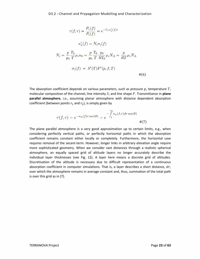
more sophisticated geometry. When we consider vast distances through a realistic spherical
atmosphere, an equally spaced grid of altitude layers no longer accurately describe the
individual layer thicknesses (see Fig. 12). A layer here means a discrete grid of altitudes.
Discretisation of the altitude is necessary due to difficult representation of a continuous
absorption coefficient in computer simulations. That is, a layer describes a short distance,
over which the atmosphere remains in average constant and, thus, summation of the total path
is over this grid as in (7).
D3.2 – Channel and Propagation Modelling and Characterization
TERRANOVA Project Page 24 of 63
Fig. 12. A path through the atmosphere where the plane parallel assumption fall short on properly explaining the structure of the atmosphere (picture of the Earth from Nasa:
NASA/NOAA/GOES Project).
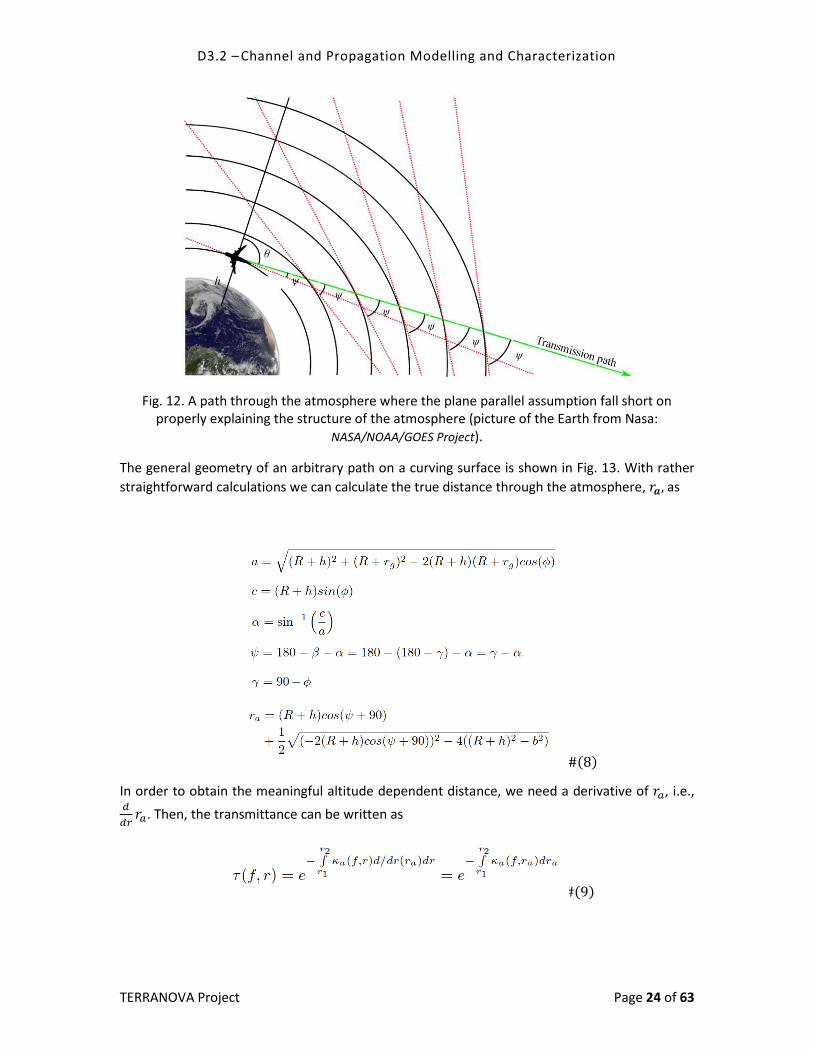
The general geometry of an arbitrary path on a curving surface is shown in Fig. 13. With rather
straightforward calculations we can calculate the true distance through the atmosphere, as
In order to obtain the meaningful altitude dependent distance, we need a derivative of , i.e.,
. Then, the transmittance can be written as
D3.2 – Channel and Propagation Modelling and Characterization
TERRANOVA Project Page 25 of 63
Fig. 13. Geometry of a general path through the atmosphere (picture of the Earth from Nasa: NASA/NOAA/GOES Project).
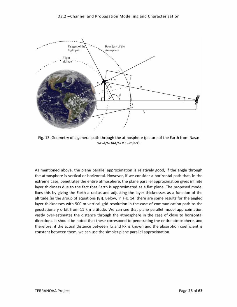
As mentioned above, the plane parallel approximation is relatively good, if the angle through
the atmosphere is vertical or horizontal. However, if we consider a horizontal path that, in the
extreme case, penetrates the entire atmosphere, the plane parallel approximation gives infinite
layer thickness due to the fact that Earth is approximated as a flat plane. The proposed model
fixes this by giving the Earth a radius and adjusting the layer thicknesses as a function of the
altitude (in the group of equations (8)). Below, in Fig. 14, there are some results for the angled
layer thicknesses with 500 m vertical grid resolution in the case of communication path to the
geostationary orbit from 11 km altitude. We can see that plane parallel model approximation
vastly over-estimates the distance through the atmosphere in the case of close to horizontal
directions. It should be noted that these correspond to penetrating the entire atmosphere, and
therefore, if the actual distance between Tx and Rx is known and the absorption coefficient is
constant between them, we can use the simpler plane parallel approximation.

D3.2 – Channel and Propagation Modelling and Characterization
TERRANOVA Project Page 26 of 63
Fig. 14. Predicted distance through the atmosphere for the plane parallel approximation and for the proposed model.
There is more to this general channel model than just geometrical issues on extremely long
distance links. Short and long distance links are all subject to atmospheric conditions that tend
to change, not only as a function of altitude, but they are also dependent on the location on
Earth. Remember that water vapor is the main cause of absorption loss in the THz band. The
amount of it varies globally due to temperature and altitude. The left-hand figure in Fig. 15 is
the mean water vapor mixing ratio and the right-hand figure is the corresponding altitude (data
from [10]).
Fig. 15. Average water vapor mixing ratio and distribution on global scale, and the mean altitude (m) of the corresponding value on the left-hand figure.
The amount of water vapor depends on the altitude via temperature, pressure, molecular
composition of the medium, all of which vary with altitude. The atmosphere is a dynamic
D3.2 – Channel and Propagation Modelling and Characterization
TERRANOVA Project Page 27 of 63
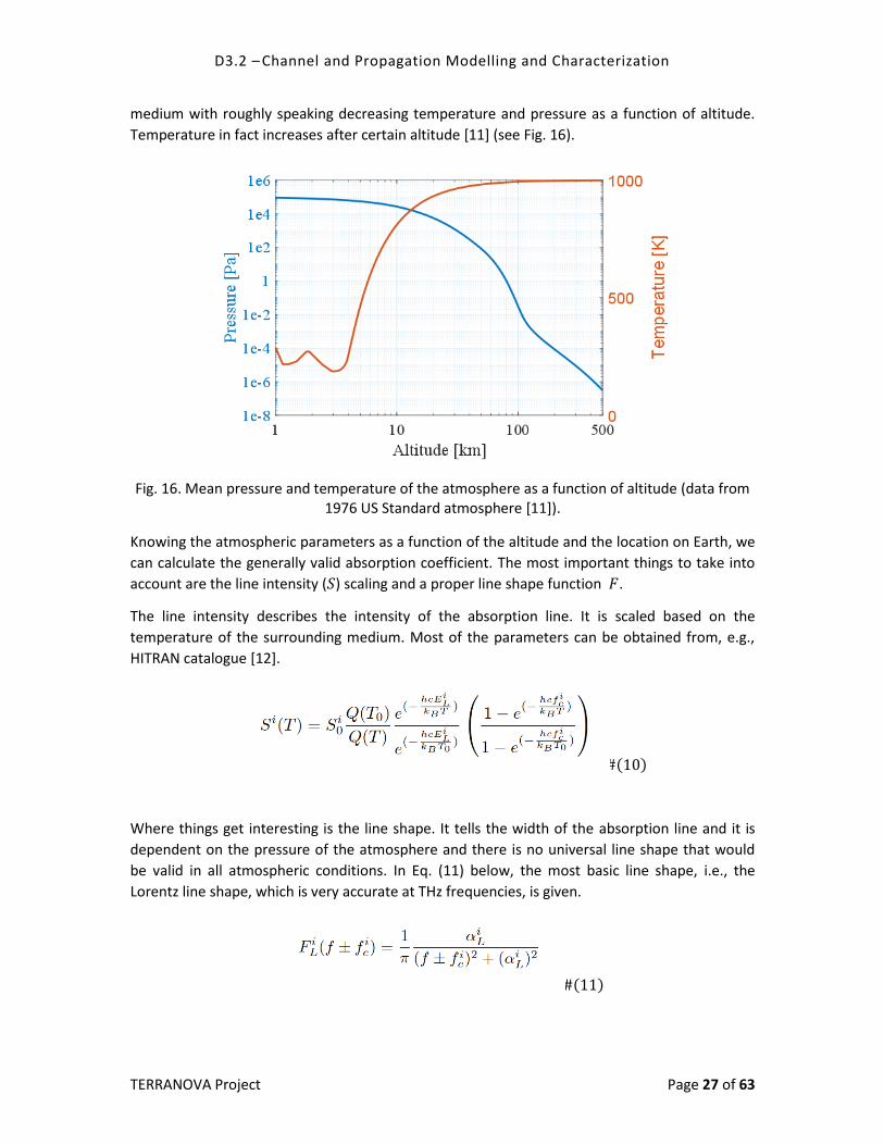
medium with roughly speaking decreasing temperature and pressure as a function of altitude.
Temperature in fact increases after certain altitude [11] (see Fig. 16).
Fig. 16. Mean pressure and temperature of the atmosphere as a function of altitude (data from 1976 US Standard atmosphere [11]).
Knowing the atmospheric parameters as a function of the altitude and the location on Earth, we
can calculate the generally valid absorption coefficient. The most important things to take into
account are the line intensity ( ) scaling and a proper line shape function .
The line intensity describes the intensity of the absorption line. It is scaled based on the
temperature of the surrounding medium. Most of the parameters can be obtained from, e.g.,
HITRAN catalogue [12].
Where things get interesting is the line shape. It tells the width of the absorption line and it is
dependent on the pressure of the atmosphere and there is no universal line shape that would
be valid in all atmospheric conditions. In Eq. (11) below, the most basic line shape, i.e., the
Lorentz line shape, which is very accurate at THz frequencies, is given.
D3.2 – Channel and Propagation Modelling and Characterization
TERRANOVA Project Page 28 of 63
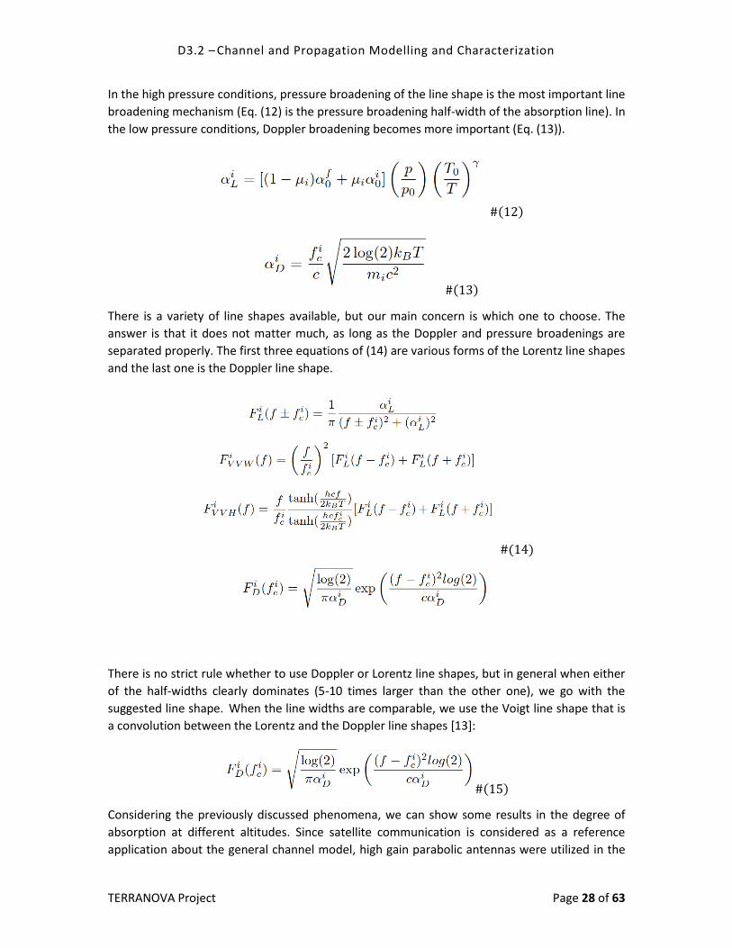
In the high pressure conditions, pressure broadening of the line shape is the most important line
broadening mechanism (Eq. (12) is the pressure broadening half-width of the absorption line). In
the low pressure conditions, Doppler broadening becomes more important (Eq. (13)).
There is a variety of line shapes available, but our main concern is which one to choose. The
answer is that it does not matter much, as long as the Doppler and pressure broadenings are
separated properly. The first three equations of (14) are various forms of the Lorentz line shapes
and the last one is the Doppler line shape.
There is no strict rule whether to use Doppler or Lorentz line shapes, but in general when either
of the half-widths clearly dominates (5-10 times larger than the other one), we go with the
suggested line shape. When the line widths are comparable, we use the Voigt line shape that is
a convolution between the Lorentz and the Doppler line shapes [13]:
Considering the previously discussed phenomena, we can show some results in the degree of
absorption at different altitudes. Since satellite communication is considered as a reference
application about the general channel model, high gain parabolic antennas were utilized in the

D3.2 – Channel and Propagation Modelling and Characterization
TERRANOVA Project Page 29 of 63
following. Fig. 17 shows per kilometer losses for fixed absorption coefficients at the given
altitude. The path losses in this equation were calculated by (16) and the antenna gains by (17).
We can see that the absorption is considerably decreased in the case of the thinner atmosphere
as one could expect.
Fig. 17. Per-kilometer losses for different altitudes.
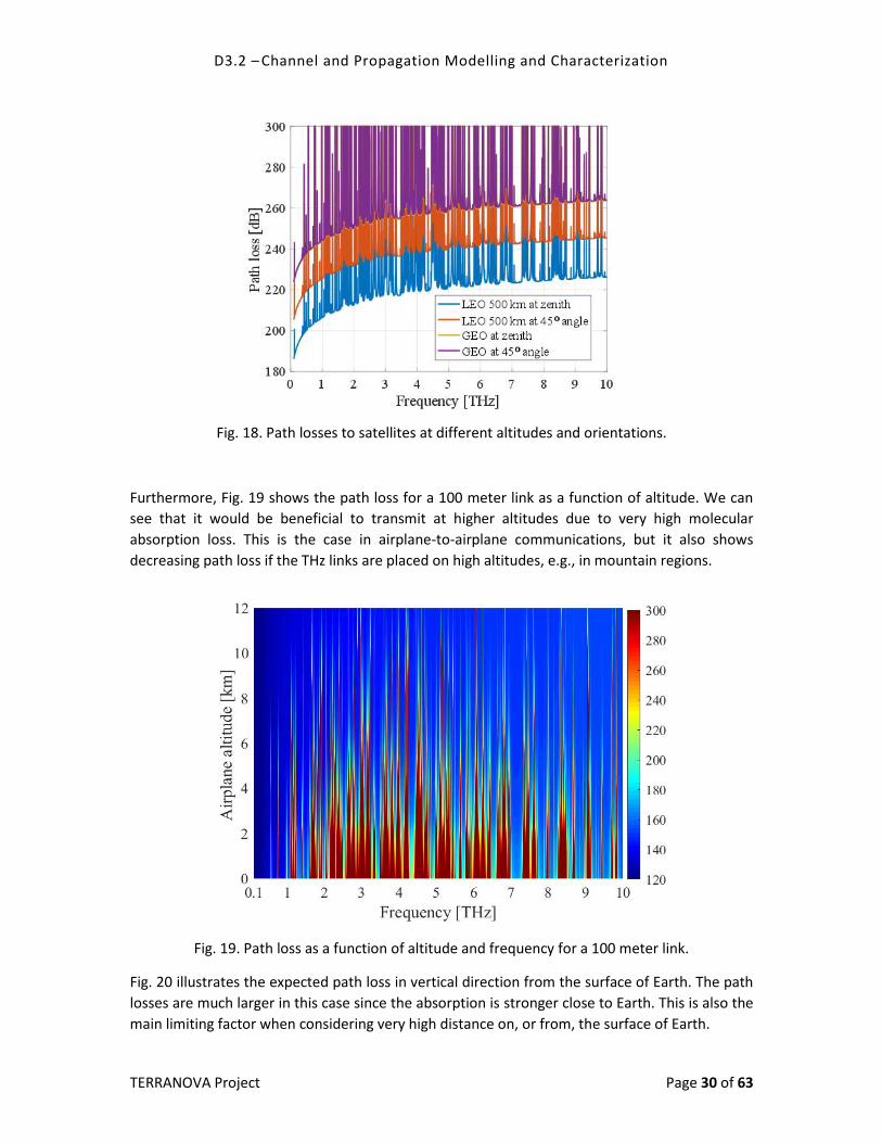
Fig. 18 shows the extreme cases of path loss through the entire atmosphere considering a path
from an airplane to satellite. Path losses become very large at long distances. However, the
numbers are decreased by the fact that airplane-to-satellite communication is considered in
contrast to the on Earth communications. The airplane altitude is 11 km. Antennas are parabolic
antennas with aperture efficiency 70%, and 1 m and 0.5 m diameter at the satellite and at the
airplane, respectively. GEO is 36,000 km away from earth, and thus, the angle is not so
important to the total distance or to the molecular absorption.
D3.2 – Channel and Propagation Modelling and Characterization
TERRANOVA Project Page 30 of 63
Fig. 18. Path losses to satellites at different altitudes and orientations.
Furthermore, Fig. 19 shows the path loss for a 100 meter link as a function of altitude. We can
see that it would be beneficial to transmit at higher altitudes due to very high molecular
absorption loss. This is the case in airplane-to-airplane communications, but it also shows
decreasing path loss if the THz links are placed on high altitudes, e.g., in mountain regions.
Fig. 19. Path loss as a function of altitude and frequency for a 100 meter link.
Fig. 20 illustrates the expected path loss in vertical direction from the surface of Earth. The path
losses are much larger in this case since the absorption is stronger close to Earth. This is also the
main limiting factor when considering very high distance on, or from, the surface of Earth.

D3.2 – Channel and Propagation Modelling and Characterization
TERRANOVA Project Page 31 of 63
Fig. 20. Path loss from ground to air as a function of frequency.
In the end, the THz band does theoretically support multigigabit-per-second links even at very
long links. Fig. 21 shows the SNRs for 500 km LEO satellite from 11 km altitude at 10 GHz with
10 mW total transmit power and target bit error probability (BEP) of . 64 QAM and BPSK
correspond to 60 and 10 Gbps (PHY). Note the high ideal antenna gains increase as a function of
frequency due to fixed physical aperture.
Fig. 21. SNR bounds for BPSK and 64-QAM for BEP= .

D3.2 – Channel and Propagation Modelling and Characterization
TERRANOVA Project Page 32 of 63
4. SIMPLIFIED CHANNEL MODELS FOR 200 – 450 GHZ BAND
The above absorption loss models give very accurate absorption estimates given any scale of
communications. However, implementing them is rather difficult and time consuming because
of the large numbers of tabulated values required from spectroscopic databases, such as
HITRAN. To address this problem, we developed a simplified molecular absorption loss model
that only requires straightforward polynomials to estimate the absorption loss, and therefore,
the path loss. The first version of the model covered the frequency range of 200 – 400 GHz and
is further detailed in [3]. The second version of the model is more complicated, but covers the
frequency range of 200 – 450 GHz, thus, completely covers the to-be-allocated frequency range
275 – 450 GHz at World Radio Conference in 2019 (WRC2019).
4.1 Model for 200 – 400 GHz band
As it was mentioned above, we have published a paper detailing the below simplified model. In
that paper, we give a simplified molecular absorption loss model for the frequency band 275 –
400 GHz. This model, however, is valid from about 200 GHz to 400 GHz. The model is given by an
exponential loss model as [3]
where
and is the distance, is the frequency, is the water vapor mixing ratio given by
in terms of the atmospheric pressure , relative humidity , and saturated water vapor partial
pressure given by [14]
D3.2 – Channel and Propagation Modelling and Characterization
TERRANOVA Project Page 33 of 63
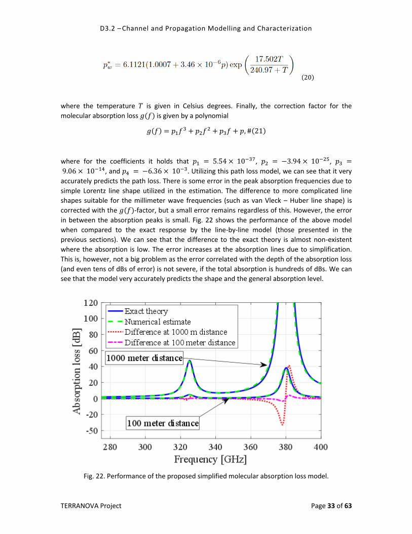
where the temperature is given in Celsius degrees. Finally, the correction factor for the
molecular absorption loss is given by a polynomial
where for the coefficients it holds that , ,
, and . Utilizing this path loss model, we can see that it very
accurately predicts the path loss. There is some error in the peak absorption frequencies due to
simple Lorentz line shape utilized in the estimation. The difference to more complicated line
shapes suitable for the millimeter wave frequencies (such as van Vleck – Huber line shape) is
corrected with the -factor, but a small error remains regardless of this. However, the error
in between the absorption peaks is small. Fig. 22 shows the performance of the above model
when compared to the exact response by the line-by-line model (those presented in the
previous sections). We can see that the difference to the exact theory is almost non-existent
where the absorption is low. The error increases at the absorption lines due to simplification.
This is, however, not a big problem as the error correlated with the depth of the absorption loss
(and even tens of dBs of error) is not severe, if the total absorption is hundreds of dBs. We can
see that the model very accurately predicts the shape and the general absorption level.
Fig. 22. Performance of the proposed simplified molecular absorption loss model.

D3.2 – Channel and Propagation Modelling and Characterization
TERRANOVA Project Page 34 of 63
ITU-R has also presented simplified channel models for the millimeter wave frequencies [15].
However, those are not as accurate as the one presented here. They are also much more
complex, as they require at minimum 9 polynomials in comparison to the three in our model.
One of the reasons for poor accuracy of the ITU-models is the assumption of the (modified) full
Lorentz line shape that is not absolutely correct for the millimeter frequencies. Figs. 23 and 24
show the difference between different ITU models and our model, as well as to the exact model
presented by our HITRAN database –based line-by-line model. We can see that the proposed
model is very close to the actual response given by ‘Theoretical van Vleck – Weisskopf’ and, for
water, by ‘Theoretical VVH – water’. In fact, the ITU model fails in the so called transmission
windows (i.e., low loss windows between the absorption lines) by over-estimating the loss. This
is particularly important in the case of long distance links. More information about the
differences between the models is given in [3].
Fig. 23. Performance of the proposed simplified molecular absorption loss model compared to other models.

D3.2 – Channel and Propagation Modelling and Characterization
TERRANOVA Project Page 35 of 63
Fig. 24. Close-up of Fig. 23 at 300 – 400 GHz band.
4.2 Model for 200 – 450 GHz band
The above model was further enhanced to cover the frequency range of 200 – 450 GHz. This
required more polynomials. Thus, it is easier to use the model of Section 4.1, if frequencies
below 400 GHz are considered. Above 400 GHz, the number of absorption lines increases fast.
Above 450 GHz, it is already simpler to use database-based approaches rather than any
polynomial-based solutions.
The LOS path loss can be given as
where is the transmittance, is the frequency, is the distance, is the water vapor
mixing ratio, is the speed of light, and are the antenna gains. Transmittance can be
estimated based on the simplified model:
D3.2 – Channel and Propagation Modelling and Characterization
TERRANOVA Project Page 36 of 63
where ) is the absorption coefficient of the th absorption line in the simplified model,
and is the fitting function for the simplified model. The absorption coefficients are as
follows:
where
and 1/cm, 1/cm, 1/cm, 1/cm,
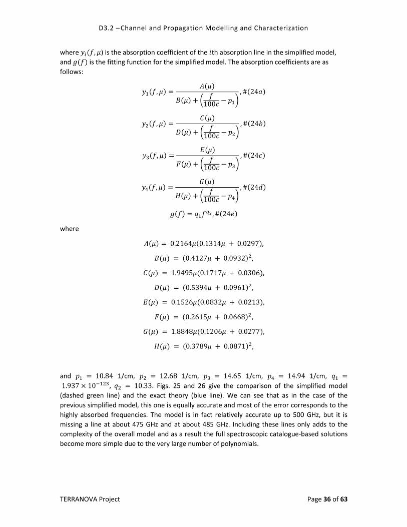
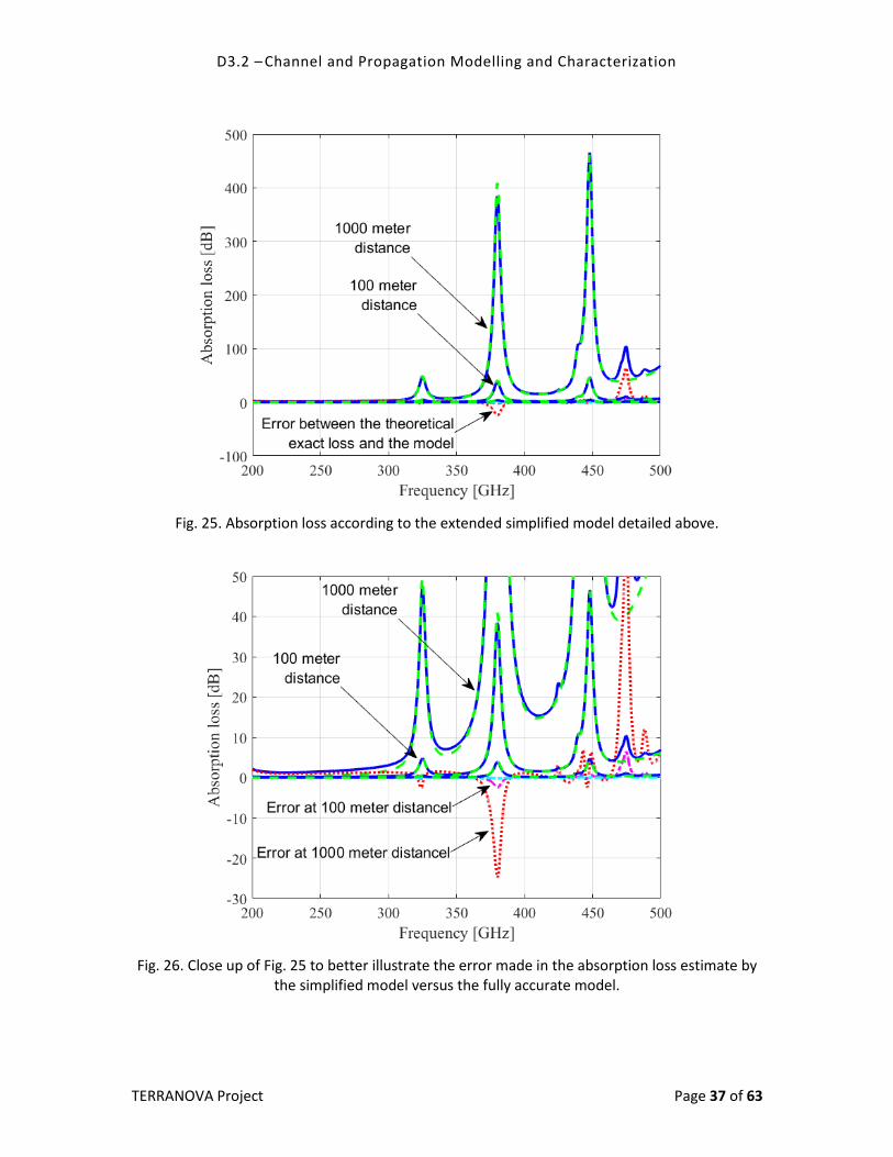
, . Figs. 25 and 26 give the comparison of the simplified model
(dashed green line) and the exact theory (blue line). We can see that as in the case of the
previous simplified model, this one is equally accurate and most of the error corresponds to the
highly absorbed frequencies. The model is in fact relatively accurate up to 500 GHz, but it is
missing a line at about 475 GHz and at about 485 GHz. Including these lines only adds to the
complexity of the overall model and as a result the full spectroscopic catalogue-based solutions
become more simple due to the very large number of polynomials.
D3.2 – Channel and Propagation Modelling and Characterization
TERRANOVA Project Page 37 of 63
Fig. 25. Absorption loss according to the extended simplified model detailed above.
Fig. 26. Close up of Fig. 25 to better illustrate the error made in the absorption loss estimate by the simplified model versus the fully accurate model.

D3.2 – Channel and Propagation Modelling and Characterization
TERRANOVA Project Page 38 of 63
5. TRANSMISSION WINDOWS BELOW ONE TERAHERTZ
As shown in the previous section, the molecular absorption coefficient causes strong signal loss
in certain deterministic frequencies. The low loss areas between the absorption lines are often
referred to as transmission windows. The molecular absorption loss increases as a function of
distance that causes these windows to shrink as the distance increases. This section considers
the available bands below one terahertz frequency. Furthermore, a model to estimate the
windows at the frequency band 200 – 400 GHz is given.
5.1 Transmission windows in the 0.275 – 1 THz band
The major transmission window centre frequencies in the 0.275 – 1 THz band are 290, 342, 410,
464, 482, 492, 651, 671, 850, and 870 GHz. However, it should be noted that due to the variable
strength of the molecular absorption loss, the specific bands may be chosen differently. The
particular centre frequencies are also subject to the considered application. The ones listed
above give a general view of the available bands in the 0.275 – 1 THz band.
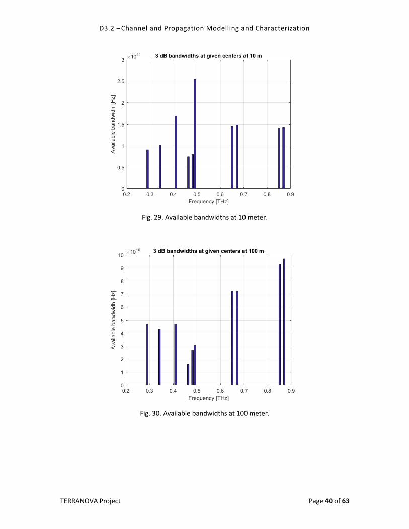
Figs. 27 and 28 show the overall LOS path loss and illustrate the possible occupied bands with
given centre frequencies. Figs. 29 and 30 further give the actual available 3 dB bandwidths
(maximum loss deviation with respect to the loss at the center frequency). The figures are given
for 10 and 100 meter distances that show the impact of the molecular absorption to the
available band very well. As the distance increases, the available spectrum becomes more and
more scarce.
As stated above, the application specific centre frequencies and target link distances, as well as
the capabilities of the utilized transceivers, play a major role in band selection. Short distance
links do not require as much planning as long distance applications, such as backhaul links. As
the distance increases, the path loss increases vastly with the following decrease of utilizable
bandwidths. This introduces some limits on the link budgets depending on the requirements of
the system. In the next section, the bandwidth estimates are looked more closely for the
frequency band of 200 – 400 GHz.
D3.2 – Channel and Propagation Modelling and Characterization
TERRANOVA Project Page 39 of 63
Fig. 27. Path loss and transmission windows at 10 meter.
Fig. 28. Path loss and transmission windows at 100 meter.
D3.2 – Channel and Propagation Modelling and Characterization
TERRANOVA Project Page 40 of 63
Fig. 29. Available bandwidths at 10 meter.
Fig. 30. Available bandwidths at 100 meter.

D3.2 – Channel and Propagation Modelling and Characterization
TERRANOVA Project Page 41 of 63
5.2 Simplified estimate for 200 – 400 GHz band
In [3], we presented a simplified model to estimate the bandwidths within the transmission
windows between the peak absorption lines. These transmission windows refer to the low loss
spectrum between the strong absorption lines. The derived model is given in terms of the
frequency deviations from the peak absorption frequencies given certain path loss threshold ,
i.e., given a maximum tolerable loss with respect to the center frequency , we can
calculate the bandwidth based on the following model
In this model, and represent the frequency deviations from 325 and 380 GHz absorption
lines for the given loss threshold . Given the above frequency deviations, we can calculate the
available bandwidths as
where is the center frequency of the higher absorption line at 380 GHz,
is the center
frequency of the lower absorption line at 325 GHz.Moreover, gives the minimum
bandwidth when the loss is limited from a single side, i.e., the bandwidth is limited by the higher
wing loss with respect to the center frequency (note that the line center in hand depends on
) and gives the maximum available bandwidth given that the band is limited from
both sides, i.e., this gives the maximum bandwidth between two absorption lines. Detailed
description of the model can be found in [3].
Figs. 31 – 34 give some results for the available bandwidths assuming a transmit center
frequency of 342 GHz. This center frequency was chosen for these examples, because it lies
between the two absorption lines in the given band (275 – 400 GHz) and this particular
frequency gives the minimum loss between these lines. Fig. 31 gives the estimated bandwidths
for three different distances and two relative humidity values. Fig. 32 gives the bandwidth
progression as a function of the distance. We can see that as the distance increases, the
exponentially increasing path loss decreases the bandwidth that can be utilized. Furthermore,
the amount of water vapor in the atmosphere also has an impact on the progression; the more
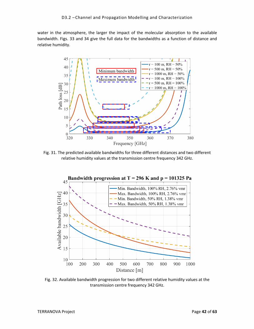
D3.2 – Channel and Propagation Modelling and Characterization
TERRANOVA Project Page 42 of 63
water in the atmosphere, the larger the impact of the molecular absorption to the available
bandwidth. Figs. 33 and 34 give the full data for the bandwidths as a function of distance and
relative humidity.
Fig. 31. The predicted available bandwidths for three different distances and two different relative humidity values at the transmission centre frequency 342 GHz.
Fig. 32. Available bandwidth progression for two different relative humidity values at the transmission centre frequency 342 GHz.

D3.2 – Channel and Propagation Modelling and Characterization
TERRANOVA Project Page 43 of 63
Fig. 33. Minimum bandwidth as a function of frequency and relative humidity at the transmission centre frequency 342 GHz.
Fig. 34. Maximum bandwidth as a function of frequency and relative humidity at the transmission centre frequency 342 GHz.

D3.2 – Channel and Propagation Modelling and Characterization
TERRANOVA Project Page 44 of 63
6. THE CHANNEL MEASUREMENTS
The channel measurements in TERRANOVA were focused on the material characterisation,
namely, on reflection and scattering properties of various common indoor materials. The
measured values were fitted to Fresnel equations [16] and scattering theories presented by
Degli-Esposti [17]. The refractive indices below have been reported in a conference paper to be
presented in September 2018 [18].
The reflection properties of different materials are important with respect to multipath
propagation modelling. It has been shown in the past that the reflections are the most potential
and utilizable NLOS communication paths in THz frequencies [19]. Therefore, the reflected paths
can enable communications even if the LOS path is blocked. The scattered paths, on the other
hand, have far more severe path loss that reduces their usability in communications. However,
given large numbers of scattering points, they may introduce additional interference. Therefore,
they are also forth to study even if the expectedly highly direction antennas will reduce the
number of unpredicted paths.
6.1 The Measurement setup
The measurements were conducted with the TeraView TeraPulse 4000 time domain
spectroscopy platform. The measurement setup is shown in Fig. 35. This measurement device is
capable of measuring frequencies from 0.1 to 4.5 THz. However, in NLOS measurements, the
maximum measureable frequencies are around 2 THz due to usually increasing path loss as a
function of frequency. More information on the measurement setup can be found in [18].
The measured materials can be seen Fig. 36 and have been also listed in Tables 2 and 3. Those
include common materials found in indoor locations, such as different wood materials with
different surfaces (painted, laminated, non-finished). Based on the given materials, indoor
simulation models are possible as these (or similar materials) give quite a good overview of the
signal behaviour on reflected and scattered paths. More information on the materials can be
found in [18].

D3.2 – Channel and Propagation Modelling and Characterization
TERRANOVA Project Page 45 of 63
Fig. 35: TeraView TeraPulse measurement setup.
Fig. 36: Measured materials.

D3.2 – Channel and Propagation Modelling and Characterization
TERRANOVA Project Page 46 of 63
6.2 Theoretical reflection loss
The theoretical reflection loss on smooth surface is given by the Fresnel equations [16]. The
Fresnel equations can be found in [16] [18] and they depend on the refractive indices of the
surface material and the angle of incidence of the incoming radiation.
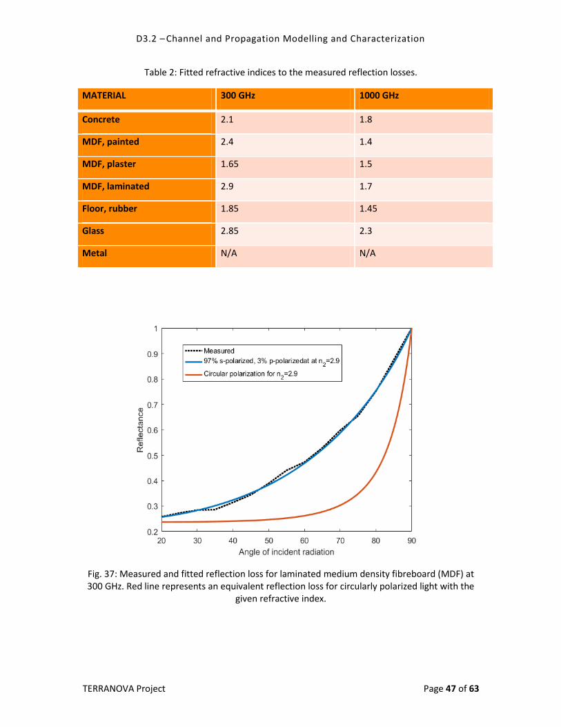
The measured reflection losses were fitted to those given by the Fresnel equations to find the
refractive indices of the materials. Those are listed in Table 2 for 300 and 1000 GHz frequencies.
An example of the fitting process is given in Fig. 37 for laminated medium density fibreboard at
300 GHz frequency. The measurement device quite strongly polarized the radiation. The best fit
was found weighting the Fresnel equations by 97% s-polarized and 3% p-polarized. Fig. 37 shows
a perfect fit between the measured and theoretical reflection loss. The red curve in the figure is
plotted in order to show the equivalent reflection loss of a circularly polarized source.
We were unable to fit the aluminium sample to the Fresnel equations due to very large reflected
power. Metals are almost like mirrors in the THz band, reflecting most of the incoming power.
Therefore, metals can be assumed to have very low reflection loss with most of the power
disappearing due to scattering on the surface imperfections.
D3.2 – Channel and Propagation Modelling and Characterization
TERRANOVA Project Page 47 of 63
Table 2: Fitted refractive indices to the measured reflection losses.
MATERIAL 300 GHz 1000 GHz
Concrete 2.1 1.8
MDF, painted 2.4 1.4
MDF, plaster 1.65 1.5
MDF, laminated 2.9 1.7
Floor, rubber 1.85 1.45
Glass 2.85 2.3
Metal N/A N/A
Fig. 37: Measured and fitted reflection loss for laminated medium density fibreboard (MDF) at 300 GHz. Red line represents an equivalent reflection loss for circularly polarized light with the
given refractive index.

D3.2 – Channel and Propagation Modelling and Characterization
TERRANOVA Project Page 48 of 63
6.3 Theoretical scattering loss
The theoretical scattering loss was modelled by the scattering model given by Degli-Esposti in
[17]. This model depends on the angle of incident radiation and the surface properties, such as
surface roughness and directivity of the outgoing radiation . Those are listed in Table 3
following the models in [17].
Fig. 38 shows an example of the scattering on plaster at 300 GHz at 45 degree angle of
incidence. It can be seen that the calculated values provide very accurate estimate of the
scattering power. It should be noted that the main lobe is wider in the measurements due to the
transmitted beam width that has been manipulated by mirrors. This causes the LOS paths to
exist at a few degrees offset between the transmitter and receiver. The theory, on the other
hand, assumed a small surface element that is evenly illuminated. As a consequence, the main
lobe appears narrower in the theoretical approach. It can be seen that the scattered power is
significantly lower than the reflected power (at minimum 30 dB). This causes the measured
scattering to be partly corrupted by thermal noise, which also shows that the scattering is not as
much a significant source of power as the reflected paths. However, the large number of
scattered rays, e.g., in the vicinity of the reflected path, may possibly cause some interference
due to the random phase of the scattering field. The corresponding equations for the considered
and fitted variables can be found in [17].
Table 3: Parameters for the scattering loss of the measured materials.
MATERIAL [cm]
Concrete 0.008 50
MDF, painted 0.004 40
MDF, plaster 0.008 50
MDF, laminated 0.001 40
Floor, rubber 0.002 40
Glass 0.002 170
Metal 0.002 170
D3.2 – Channel and Propagation Modelling and Characterization
TERRANOVA Project Page 49 of 63
Fig. 38: Measured and theoretical scattering and reflection loss for plaster at 300 GHz at 45 degree incidence angle.
D3.2 – Channel and Propagation Modelling and Characterization
TERRANOVA Project Page 50 of 63
7. NOISE IN THE THZ BAND
The noise present in the THz band is mostly due to the thermal noise of the receiver equipment.
However, theoretically, there is also increased noise due to the antenna brightness temperature
and re-radiation of the absorbed energy from own transmissions (self-induced noise). The
former is explained below in more detail. The self-induced noise has been predicted to cause
significant noise in the THz frequencies. However, we wrote a paper earlier analysing this noise
and concluded that it is most likely unmeasurable because it is so weak that regular thermal
noise dominates [20]. We have also tried to measure this type of noise, but the conclusions in
[20] seem to be correct and we have been unable to capture anything apart from the thermal
noise itself. For these reasons, we can safely utilize the regular thermal noise in estimating the
overall noise level in THz systems.
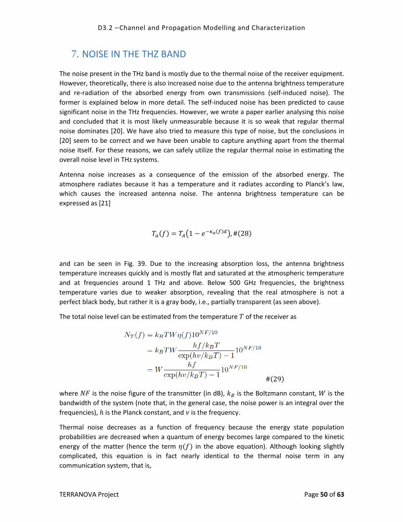
Antenna noise increases as a consequence of the emission of the absorbed energy. The
atmosphere radiates because it has a temperature and it radiates according to Planck’s law,
which causes the increased antenna noise. The antenna brightness temperature can be
expressed as [21]
and can be seen in Fig. 39. Due to the increasing absorption loss, the antenna brightness
temperature increases quickly and is mostly flat and saturated at the atmospheric temperature
and at frequencies around 1 THz and above. Below 500 GHz frequencies, the brightness
temperature varies due to weaker absorption, revealing that the real atmosphere is not a
perfect black body, but rather it is a gray body, i.e., partially transparent (as seen above).
The total noise level can be estimated from the temperature of the receiver as
where is the noise figure of the transmitter (in dB), is the Boltzmann constant, is the
bandwidth of the system (note that, in the general case, the noise power is an integral over the
frequencies), is the Planck constant, and is the frequency.
Thermal noise decreases as a function of frequency because the energy state population
probabilities are decreased when a quantum of energy becomes large compared to the kinetic
energy of the matter (hence the term in the above equation). Although looking slightly
complicated, this equation is in fact nearly identical to the thermal noise term in any
communication system, that is,

D3.2 – Channel and Propagation Modelling and Characterization
TERRANOVA Project Page 51 of 63
Fig 39. Antenna brightness temperature as a function of frequency.

D3.2 – Channel and Propagation Modelling and Characterization
TERRANOVA Project Page 52 of 63
8. FADING IN THZ BAND
The fading characteristics and models for the THz band will be investigated in TERRANOVA
project. The main work on those will be conducted by the simulation models, while the fading
will be investigated in future work. The utilized simulation models are discussed in the next
section and a short literature review will be given below.
The LOS and NLOS channel models were discussed above. All the channel effects can be
considered as part of the large and small scale fading. Especially, the molecular absorption loss
can be viewed as a deterministic fading process dependent on the distance. In general, the THz
channel particularities have been investigated in several works. In more detail, in [6], the
authors presented a deterministic propagation model for electromagnetic nanoscale
communications in the THz band, based on radiative transfer theory. In addition, in [3], a
simplified path-loss model for the 275-400 GHz band was introduced, which was employed in [4]
in order to evaluate the THz link performance in terms of average signal-to-noise ratio (SNR) and
capacity. Furthermore, in [1], a multi-ray THz propagation model was presented, whereas, in
[22], the authors reported a path-loss model for nano-sensor networks operating in the THz
band for plant foliage applications. In [23], a propagation model for intra-body nano-scale
communications was provided and in [24], a multi-ray THz propagation model was presented.
Although all the above mentioned contributions revealed the particularities of the THz medium,
they neglected the impact of fading. In [25], [26] and [27], the authors presented suitable
stochastic models that are able to accommodate the multipath fading effect in the THz band. In
particular, in [25], the authors introduced a multi-path THz channel model where the
attenuation factor was modelled as a Rayleigh or Nakagami-m distribution under the non-line-
of- sight condition and as a Rician or Nakagami-m distribution in LOS conditions. Moreover, in
[26] and [27], the authors proposed a two dimensional geometrical propagation model for
indoor THz communications. Based on this model, they developed a parametric reference model
for a THz multi-path Rician fading channel. In [28], the influence of antenna directivities on the
THz indoor channels for various antenna types was investigated assuming Rician fading,
whereas, in [29], the authors used a log-distance shadowing path-loss model for THz nano-
sensor networks communications in vegetation.
None of these models give definite answers on the nature of fading, and especially on the small
scale fading characteristics of the THz band. Therefore, the fading research is part of the
TERRANOVA project. As mentioned above, the fading is studied with the simulation models
presented in the next section, where also some very preliminary results on the received
multipath signals are given.
D3.2 – Channel and Propagation Modelling and Characterization
TERRANOVA Project Page 53 of 63
9. SIMULATION FOR STUDYING FADING, INTERFERENCE, AND
MULTIPATH PROPAGATION
The simulation models assist the study of mathematically difficult multipath and multiuser
models. In TERRANOVA project, two simulation approaches have been developed, a ray-tracing
model presented in Section 9.1 and a geometrical approach presented in Section 9.2. These
models incorporate the LOS and NLOS models presented in this document. Those include the
reflection and scattering models parameterized by the empirical measurements, the theoretical
LOS model, and the noise. Although the simulation models help understand the channel
behavior and limits placed by the large number of multipath signals from many Txs, they also
make it possible to study fading. An example on this is given in Section 9.2.
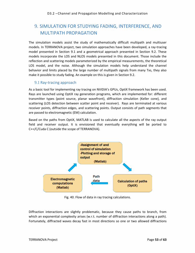
9.1 Ray-tracing approach
As a basic tool for implementing ray tracing on NVIDIA’s GPUs, OptiX framework has been used.
Rays are launched using OptiX ray generation programs, which are implemented for: different
transmitter types (point source, planar wavefront), diffraction simulation (Keller cone), and
scattering (LOS detection between scatter point and receiver). Rays are terminated at various
receiver points, diffraction edges, and scattering points. Output consists of path segments that
are passed to electromagnetic (EM) calculation.
Based on the paths from OptiX, MATLAB is used to calculate all the aspects of the ray output
field and receiver output. It is envisioned that eventually everything will be ported to
C++/C/Cuda C (outside the scope of TERRANOVA).
Fig. 40. Flow of data in ray tracing calculations.
Diffraction interactions are slightly problematic, because they cause paths to branch, from
which an exponential complexity arises (w.r.t. number of diffraction interactions along a path).
Fortunately, diffracted waves decay fast in most directions so one or two allowed diffractions

D3.2 – Channel and Propagation Modelling and Characterization
TERRANOVA Project Page 54 of 63
along a path are enough. The uniform theory of diffraction (UTD) is used for all the diffraction
field evaluations and classical Fresnel equations used for reflections.
Earlier solution from UOULU was developed further in TERRANOVA including support for diffuse
scatter simulation and improved geometry / material handling. Regarding scattering, the last
interaction point of a ray path before it hits a receiver will be considered as a significant
scattering interaction. The path may experience multiple reflections and/or some diffractions
before this scattering point. Scattering is modelled by Degli-Esposti’s model [17]. In
TERRANOVA, measurements were done to obtain the scattering model parameters for various
materials found in a typical office room.
Fig. 41. Office room (adapted from [30]) with four transmitters (in the corners close to roof) and 35 possible locations for a receiver. Different colours indicate different materials (concrete,
glass, painted wood, rubber floor, laminated MDF).

D3.2 – Channel and Propagation Modelling and Characterization
TERRANOVA Project Page 55 of 63
Fig. 42. Scatter points in the office room.
Fig. 43. Delay spread as a function of beam angle for receivers 1, 15, and 30. Center frequency is equal to 300 GHz.

D3.2 – Channel and Propagation Modelling and Characterization
TERRANOVA Project Page 56 of 63
Fig. 43 shows the delay spread as a function of beam angle for receivers in three different
positions. It can be seen that when beam angles are less than 20 degrees, channel is essentially
LOS. In this calculation, the best transmitter (out of the 4 possible in the room corners) and the
best beam pointing direction have been found for each receiver (not necessarily LOS direction
although almost always it was like this). It is emphasized that the results in Fig. 43 are based on
universally valid theories utilizing actual measured parameters for different materials at THz
frequencies.
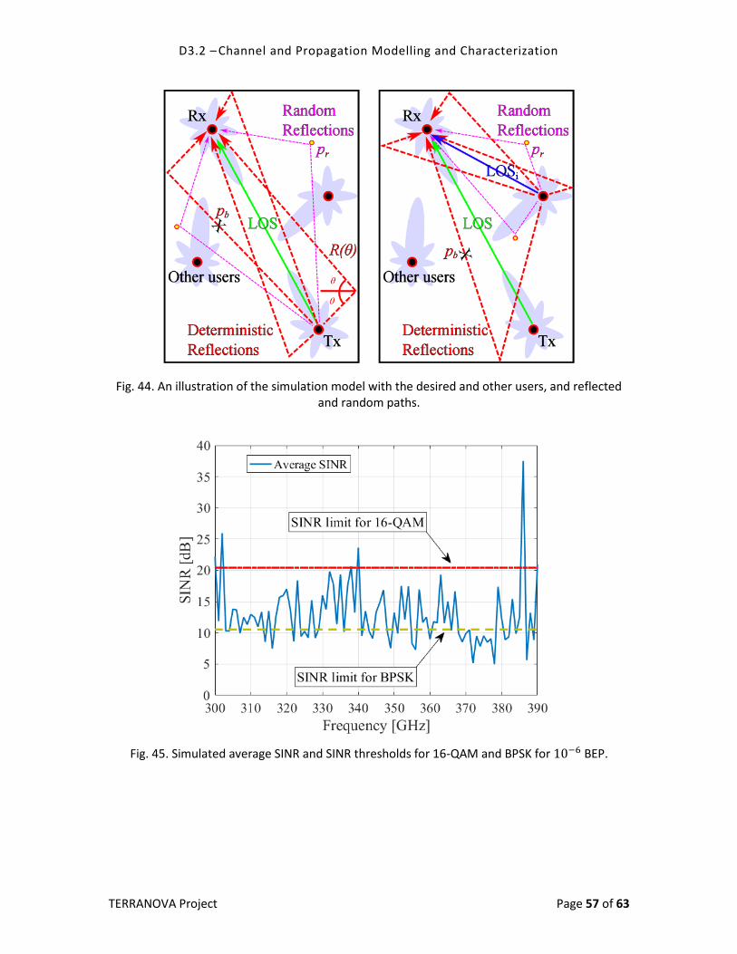
9.2 Geometric simulation model
The geometric simulation model is based on modelling the environment as a set of deterministic
and random objects. In the early phase, the deterministic objects are walls, floor, and ceiling.
The random objects are furniture and other objects of the environment (coffee mugs, screens,
surface irregularities, etc.). The random objects and their locations are randomized on every
drop, as are the other users. The deterministic signal paths are calculated from the reflections
on the walls, floor, and ceiling, and the random objects operate as reflectors or scatterers. The
possible signal paths are shown in Fig. 44 for the desired user (left-hand figure) and for the other
users (right-hand figure). Furthermore, all the paths are subject to certain blocking probability as
it is unlikely that all the deterministic paths are available due to possible furniture or humans
blocking the signals.
The idea of the geometric simulator is similar to ray tracing, but the difference is due to the
random paths. They are different for all the drops of the simulation (one drop is one network
realization for which the channels are calculated). This gives variability to the received signals
due to movement of the user. The next step of the development is to determine the time
domain, which gives an opportunity to study, for instance, fading and medium access control
(MAC) solutions. The simulator has been developed to be as generic as possible, so that fixed
objects, channel models, antennas, etc. can easily be incorporated.
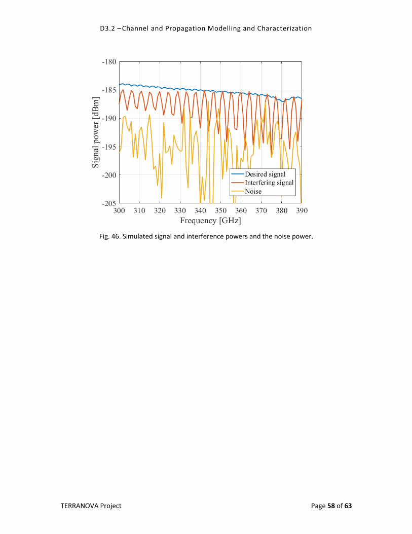
Figs. 45 and 46 give an example of simulation results for a situation similar to Fig. 44. This
simulation was run and averaged over 10 drops with 50 other users and 50 random objects
(both Poisson distributed) in a 10-by-10-by-3 room, ALOHA MAC with 50% transmit
probability, 50% blocking probability, and 45 degree wide conical shaped antenna patterns for
the Txs and Rxs (random directions). The test case is a very dense network, but it also shows the
impact of the interference very well. The fading over frequencies becomes large enough to
prevent the usage of even simple modulations with BPSK performance already struggling with
BEP target. This kind of results are required when estimating the fading (small and large
scale) in multipath and multiuser channels. However, as stated above, this simulator is still a
work in progress and will be documented and utilized in the future work.
D3.2 – Channel and Propagation Modelling and Characterization
TERRANOVA Project Page 57 of 63
Fig. 44. An illustration of the simulation model with the desired and other users, and reflected and random paths.
Fig. 45. Simulated average SINR and SINR thresholds for 16-QAM and BPSK for BEP.
D3.2 – Channel and Propagation Modelling and Characterization
TERRANOVA Project Page 58 of 63
Fig. 46. Simulated signal and interference powers and the noise power.

D3.2 – Channel and Propagation Modelling and Characterization
TERRANOVA Project Page 59 of 63
10. FUTURE WORK
Work on the WP3 T3.1 is scheduled to continue until the end of the 2018 (M18 of TERRANOVA
project). This deliverable is due in the end of August 2018 (M14). Therefore, the work on the
channel model continues beyond this document. The remaining four months of work will
include finalizing the derived channel models and gathering more data by measurements.
The main works to be concluded by the end of M18 are as follows:
Finalizing and submitting a journal article on the general LOS channel model presented
in Section 3.
Writing and submitting a journal article on the simplified channel model for the 200 –
450 GHz band presented in Section 4.2.
Measurements on the reflection and scattering coefficient for more materials in order
to form a more comprehensive database of material characteristics.
Develop the simulation tools to study and develop fading models for the THz band.
Further study on the noise processes and trying to capture the behaviour of the
molecular absorption noise by measurements.
On top of these tasks, the remaining time allows to study propagation and channel
characteristics identified by this or other work packages before the end of M18.

D3.2 – Channel and Propagation Modelling and Characterization
TERRANOVA Project Page 60 of 63
11. CONCLUSIONS
The main task of T3.1 has been to produce new and novel channel models to be utilized in the
TERRANOVA project. Those were presented in the document and include general theoretical
full-band LOS channel models as well as simplified LOS models for confined frequency bands.
The presented NLOS models, namely reflection and scattering coefficients for various materials,
can be utilized in multipath and NLOS propagation studies. By combining different models
presented herein, modelling of very complex propagation environments, such as indoor
locations, can be achieved. The backhaul links are easier, because they only require LOS channel
models along with possible rain and fog attenuation models. The average loss on LOS channels
can be estimated based on the location and altitude on Earth. The indoor locations usually have
many possible paths from Tx to Rx. These paths can be easily estimated by considering the
summation of multiple unique paths via reflection, scattering, and/or diffraction.
The interesting part of the THz communications is directional antennas. They are required due
to large path loss, but they also limit the number of possible paths from Tx to Rx. Therefore,
even closely related scenarios may have completely different propagation characteristics. For
example, indoor communication with LOS path is the most efficient. However, if it is blocked for
any reason, the NLOS paths become a viable option for communications. In any case, the
channels for all the paths can be constructed based on the channel models propagation
characteristics presented in this document.

D3.2 – Channel and Propagation Modelling and Characterization
TERRANOVA Project Page 61 of 63
REFERENCES
[1] E. N. Papasotiriou, Kokkoniemi, J., A.-A. A. Boulogeorgos, J. Lehtomäki, A. Alexiou and M.
Juntti, “A New Look to 275 to 400 GHz Band Channel Model and Performance Evaluation,”
in IEEE International Symposium on Personal, Indoor and Mobile Radio Communications,
Bologna, Italy, 2018.
[2] V. Petrov, J. Kokkoniemi, D. Moltchanov, J. Lehtomaki, Y. Koucheryavy and M. Juntti, “Last
Meter Indoor Terahertz Wireless Access: Performance Insights and Implementation
Roadmap,” [accepted] IEEE Commun. Magazine, 2018.
[3] J. Kokkoniemi, J. Lehtomäki and M. Juntti, “Simplified Molecular Absorption Loss Model for
275 - 400 Gigahertz Frequency Band,” in 12th European Conference on Antennas and
Propagation, London, 2018.
[4] A.-A. A. Boulogeorgos, E. N. Papasotiriou, J. Kokkoniemi, J. Lehtomaki, A. Alexiou and M.
Juntti, “Performance Evaluation of THz Wireless Systems Operating in 275-400 GHz Band,”
in IEEE 87th Vehicular Technology Conference: VTC2018-Spring, Porto, Portugal, 2018.
[5] S. Paine, “The am atmospheric model; SMA technical memo #152, version 9.2,”
Smithsonian Astrophysical Observatory, 2017.
[6] J. M. Jornet and I. F. Akyildiz, “Channel Modeling and Capacity Analysis for Electromagnetic
Nanonetworks in the Terahertz Band,” in IEEE Trans. Wireless Commun., vol. 10, Oct. 2011,
pp. 3211 - 3221.
[7] J. Kokkoniemi, J. Lehtomäki and M. Juntti, “Frequency and time domain channel models for
nanonetworks in terahertz band,” in IEEE Trans. Antennas Propag., vol. 63, 2015, pp. 678 -
691.
[8] “ITU-R Recommendation P.838-3, Specific attenuation model for rain for use in prediction
methods,” International Telecommunication Union Radiocommunication Sector, 2005.
[9] “ITU-R Recommendation P.840-7, Attenuation due to clouds and fog,” International
Telecommunication Union Radiocommunication Sector, 2017.
[10] “MERRA-2 instM_3d_ana_Np: 3d, Monthly mean, Instantaneous, Pressure-Level, Analysis,
Analyzed Meteorological Fields V5.12.4,” Global Modeling and Assimilation Office (GMAO),
Goddard Earth Sciences Data and Information Services Center (GES DISC), 2015.
[11] “U.S. standard atmosphere, 1976,” National Aeronatics and Space Administration,
D3.2 – Channel and Propagation Modelling and Characterization
TERRANOVA Project Page 62 of 63
Washington D.C., 1976.
[12] I. E. Gordon, L. S. Rothman, C. Hill and e. al., “The HITRAN2016 Molecular Spectroscopic
Database,” J Quant. Spectrosc. Radiat. Transfer, vol. 203, no. December 2017, pp. 3 - 69,
2017.
[13] X. Huang and Y. L. Yung, “A common misunderstanding about the Voigt line profile,” J.
Atmos. Sci., vol. 61, pp. 1630 - 1632, 2004.
[14] O. A. Alduchov and R. E. Eskridge, “Improved magnus form approximation of saturation
vapor pressure,” J. Appl. Meteor., vol. 35, no. 4, pp. 601 - 609, 1996.
[15] “ITU-R Recommendation P-676-8: Attenuation by atmospheric gases,” International
Telecommunication Union Radiocommunication Sector, 2009.
[16] A. I. Lvovsky, “Fresnel Equations,” in Encyclopedia of Optical Engineering, New York, Taylor
and Francis, 2013, pp. 1-6.
[17] V. Degli-Esposti, F. Fuschini, E. M. Vitucci and G. Falciasecca, “Measurement and Modelling
of Scattering From Buildings,” IEEE Transactions on Antennas and Propagation, vol. 55, no.
1, pp. 143-153, 2007.
[18] J. Kokkoniemi, J. Lehtomäki and M. Juntti, “Reflection Coefficients for Common Indoor
Materials in the Terahertz Band,” in [accepted] ACM NanoCom, Reykjavik, Iceland., 2018.
[19] J. Kokkoniemi, V. Petrov, D. Moltchanov, J. Lehtomäki, Y. Koucheryavy and M. Juntti,
“Wideband Terahertz Band Reflection and Diffuse Scattering Measurements for Beyond 5G
Indoor Wireless Networks,” in European Wireless, Oulu, 2016.
[20] J. Kokkoniemi, J. Lehtomäki and M. Juntti, “A discussion on molecular absorption noise in
the terahertz band,” vol. 8, no. June 2016, pp. 35 - 45, 2016.
[21] “ITU-R Recommendation P.372-13, Radio noise,” International Telecommunication Union
Radiocommunication Sector, 2016.
[22] A. Afsharinejad, A. Davy, B. Jennings and C. Brennan, “An initial path-loss model within
vegetation in the THz band,” in 9th European Conference on Antennas and Propagation,
Lisbon, Portugal, 2015.
[23] H. Elayan, R. M. Shubair, J. M. Jornet and P. Johari, “Terahertz channel model and link
budget analysis for intrabody nanoscale communication,” IEEE Trans. Nanobioscience, vol.
16, no. 6, pp. 491-503, Sep. 2017.
[24] C. Han, A. O. Bicen and I. F. Akyildiz, “Multi-raychannelmodelingand wideband
characterization for wireless communications in the terahertz band,” IEEE Trans. Wireless
Commun., vol. 14, no. 5, pp. 2402-2412, May 2015.

D3.2 – Channel and Propagation Modelling and Characterization
TERRANOVA Project Page 63 of 63
[25] A. R. Ekti, A. Boyaci and A. Alparslan et al., “Statistical modeling of propagation channels for
terahertz band,” in IEEE Conference on Standards for Communications and Networking,
Helsinki, Finland, 2017.
[26] S. Kim and A. Zajic, “Statistical modeling of THz scatter channels,” in European Conference
on Antennas and Propagation, Lisbon, Portugal, 2015.
[27] S. Kim. and A. Zajic, “Statistical modeling and simulation of short-range device-to-device
communication channels at sub-THz frequencies,” IEEE Trans. Wireless Commun., vol. 15,
no. 9, pp. 6423-6433, Sep. 2016.
[28] S. Priebe, M. Jacob and T. Kürner, “The impact of antenna directivities on THz indoor
channel characteristics,” in European Conference on Antennas and Propagation, Prague,
Czech Republic, 2012.
[29] A. Afsharinejad, A. Davy, B. Jennings, S. Rasmann and C. Brennan, “A path-loss model
incorporating shadowing for THz band propagation in vegetation,” in IEEE Global
Communications Conference, San Diego, CA, USA, 2015.
[30] Z.-Y. Liu, L.-X. Guo and X. Meng, “Efficient three-dimensional ray-tracing model for
electromagnetic propagation prediction in complex indoor environments,” J. Opt. Soc. Am.,
vol. A30, pp. 1654-1660, 2013.