deloitte marketpoint. analysis of economic impact of lng

Deloitte MarketPoint.

Analysis of Economic Impact of LNG Exports

from the United States

i

Contents

Executive summary 1

Overview of Deloitte MarketPoint Reference Case 5

Potential impact of LNG exports 10

Comparison of results to other studies 18

Appendix A: Price Impact Charts for other Export Cases 20

Appendix B: DMP’s World Gas Model and data 24

Executive summary

1

Executive summary

Deloitte MarketPoint LLC (“DMP”) has been

engaged by Excelerate Energy L.P.

("Excelerate") to provide an independent and

objective assessment of the potential economic

impacts of LNG exports from the United States.

We analyzed the impact of exports from

Excelerate’s Lavaca Bay terminal, located along

the Gulf coast of Texas, by itself and also in

combination with varying levels of LNG exports

from other locations.

A fundamental question regarding LNG exports

is: Are there sufficient domestic natural gas

supplies for both domestic consumption and

LNG exports. That is, does the U.S. need the

gas for its own consumption or does the U.S.

possess sufficiently abundant gas resources to

supply both domestic consumption and exports?

A more difficult question is: How much will U.S.

natural gas prices increase as a result of LNG

exports? To understand the possible answers to

these questions, one must consider the full

gamut of natural gas supply and demand in the

U.S. and the rest of the world and how they are

dynamically connected.

In our view, simple comparisons of total

available domestic resources to projected future

consumption are insufficient to adequately

analyze the economic impact of LNG exports.

The real issue is not one of volume, but of price

impact. In a free market economy, price is one of

the best measures of scarcity, and if price is not

significantly affected, then scarcity and shortage

of supply typically do not occur. In this report, we

demonstrate that the magnitude of domestic

price increase that results from exports of

natural gas in the form of LNG is projected to be

quite small.

However, other projections, including those

developed by the DOE’s Energy Information

Administration (EIA), estimate substantially

larger price impacts from LNG exports than

derived from our analysis. We shall compare

different projections and provide our assessment

as to why the projections differ. A key

determinant to the estimated price impact is the

supply response to increased demand including

LNG exports. To a large degree, North American

gas producers’ ability to increase productive

capacity in anticipation of LNG export volumes

will determine the price impact. After all, there is

widespread agreement of the vast size of the

North American natural gas resource base

among the various studies and yet estimated

price impacts vary widely. If one assumes that

producers will fail to keep pace with demand

growth, including LNG exports, then the price

impact of LNG exports, especially in early years

of operations, will be far greater than if they

anticipate demand and make supplies available

as they are needed. Hence, a proper model of

market supply-demand dynamics is required to

more accurately project price impacts.

DMP applied its integrated North American and

World Gas Model (WGM or Model) to analyze

the price and quantity impacts of LNG exports

on the U.S. gas market.1 The WGM projects

1 This report w as prepared for Excelerate Energy

L.P. ("Client") and should not be disclosed to, used or relied upon by any other person or entity. Deloitte

Marketpoint LLC shall not be responsible for any loss

sustained by any such use or reliance. Please note

that the analysis set forth in this report is based on the

application of economic logic and specif ic

Executive summary

2

monthly prices and quantities over a 30 year

time horizon based on demonstrated economic

theories. It includes disaggregated

representations of North America, Europe, and

other major global markets. The WGM solves for

prices and quantities simultaneously across

multiple markets and across multiple time points.

Unlike many other models which compute prices

and quantities assuming all parties work

together to achieve a single global objective,

WGM applies fundamental economic theories to

represent self-interested decisions made by

each market “agent” along each stage of the

supply chain. It rigorously adheres to accepted

microeconomic theory to solve for supply and

demand using an “agent based” approach. More

information about WGM is included in the

Appendix.

Vital to this analysis, the WGM represents

fundamental natural gas producer decisions

regarding when and how much reserves to

develop given the producer’s resource

endowments and anticipated forward prices.

This supply-demand dynamic is particularly

important in analyzing the impact of demand

changes (e.g., LNG exports) because without it,

the answer will likely greatly overestimate the

price impact. Indeed, producers will anticipate

the export volumes and make production

decisions accordingly. LNG exporters might

back up their multi-billion dollar projects with

long-term supply contracts, but even if they do

not, producers will anticipate future prices and

demand growth in their production decisions.

Missing this supply-demand dynamic is

tantamount to assuming the market will be

surprised and unprepared for the volume of

exports and have to ration fixed supplies to meet

assumptions and the results are not intended to be

predictions of events or future outcomes.

Notw ithstanding the foregoing, Client may submit this report to the U.S. Department of Energy and the

Federal Energy Regulatory Commission in support of

Client’s liquef ied natural gas “(LNG”) export

application.

the required volumes. Static models assume a

fixed supply volume (i.e., productive capacity)

during each time period and therefore are prone

to over-estimate the price impact of a demand

change. Typically, users have to override this

assumption by manually adjusting supply to

meet demand. If insufficient supply volumes are

added to meet the incremental demand, prices

could shoot up until enough supply volumes are

added to eventually catch up with demand.

Instead of a static approach, the WGM uses

sophisticated depletable resource modeling to

represent producer decisions. The model uses a

“rational expectations” approach, which

assumes that today’s drilling decisions affect

tomorrow’s price and tomorrow’s price affects

today’s drilling decisions. It captures the market

dynamics between suppliers and consumers.

It is well documented that shale gas production

has grown tremendously over the past several

years. According to the EIA, shale gas

production climbed to over 35% of the total U.S.

production in January of 20122. By comparison,

shale gas production was only about 5% of the

total U.S. production in 2006, when

improvements in shale gas production

technologies (e.g., hydraulic fracturing combined

with horizontal drilling) were starting to

significantly reduce production costs. However,

there is considerable debate as to how long this

trend will continue and how much will be

produced out of each shale gas basin. Rather

than simply extrapolating past trends, WGM

projects production based resource volumes and

costs, future gas demand, particularly for power

generation, and competition among various

sources in each market area. It computes

incremental sources to meet a change in

demand and the resulting impact on price.

2 Computed from the EIA’s Natural Gas Weekly Update for

week ending June 27, 2012.

Executive summary

3

Based on our existing model and assumptions,

which we will call the “Reference Case”, we

developed five cases with different LNG export

volumes to assess the impact of LNG exports.

The five LNG export scenarios and their

assumed export volumes by location are shown

in Figure 1. Other Gulf in the figure refers to all

other Gulf of Mexico terminals in Texas and

Louisiana besides Lavaca Bay.

All cases are identical except for the assumed

volume of LNG exports. The 1.33 Bcfd case

assumed only exports from Lavaca Bay so that

we could isolate the impact of the terminal. In

the other LNG export cases, we assumed the

Lavaca Bay terminal plus volumes from other

locations so that the total exports volume

equaled 3, 6, 9, and 12 Bcfd. The export

volumes were assumed to be constant for

twenty years from 2018 through 2037.

We represented LNG exports in the model as

demands at various model locations generally

corresponding to the locations of proposed

export terminals (e.g., Gulf Texas, Gulf

Louisiana, and Cove Point) that have applied for

a DOE export license. The cases are not

intended as forecasts of which export terminals

will be built, but rather to test the potential

impact given alternative levels of LNG exports.

Furthermore, the export volumes are assumed

to be constant over the entire 20 year period.

Since our existing model already represented

these import LNG terminals, we only had to

represent exports by adding demands near each

of the terminals. Comparing results of the five

LNG export cases to the Reference Case, we

projected how much the various levels of LNG

exports could increase domestic prices and

affect production and flows.

Given the model’s assumptions and economic

logic, the WGM projects prices and volumes for

over 200 market hubs and represents every

state in the United States. We can examine the

impact at each location and also compute a

volume-weighted average U.S. “citygate” price

by weighting price impact by state using the

state’s demand. Impact on the U.S. prices

increase along with the volume of exports.

As shown in Figure 2, the WGM’s projected

Figure 1: LNG export scenarios

Export Case

Terminal 1.33 Bcfd 3 Bcfd 6 Bcfd 9 Bcfd 12 Bcfd

Lavaca Bay 1.33 1.33 1.33 1.33 1.33

Other Gulf 1.67 4.67 6.67 9.67

Cove Point (MD)

1.0 1.0

Total 1.33 3.0 6.0 9.0 12.0

Figure 2: Potential Impact of LNG export on U.S. prices (Average 2018-37)

Export Case Average US

Citygate Henry Hub New York

1.33 Bcfd 0.4% 0.4% 0.3%

3 Bcfd 1.0% 1.7% 0.9%

6 Bcfd 2.2% 4.0% 1.9%

9 Bcfd 3.2% 5.5% 3.2%

12 Bcfd 4.3% 7.7% 4.1%

Executive summary

4

impact on average U.S. citygate prices for the

assumed years of operation (2018 to 2037)

ranged from well under 1% in the 1.33 Bcfd

(Lavaca Bay only) case to 4.3% in the 12 Bcfd

case. However, the impacts vary significantly by

location. Figure 2 shows the percentage change

relative to the Reference Case to the projected

average U.S. citygate price and at the Henry

Hub and New York prices under various LNG

export volumes.

As Figure 2 shows, the price impact is highly

dependent on location. The impact on the price

at Henry Hub, the world’s most widely used

benchmark for natural gas prices, is significantly

higher than the national average. The reason is

that the Henry Hub, located in Louisiana, is in

close proximity to the prospective export

terminals, which are primarily located in the U.S.

Gulf of Mexico region. Since there are several

cases analyzed, we will primarily describe

results of the 6 Bcfd export case since it is the

middle case. The impacts are roughly

proportional to the export volumes. In the 6 Bcfd

export case, the impact on the Henry Hub price

is an increase of 4.0% over the Reference Case.

Generally, the price impact in markets

diminishes with distance away from export

terminals as other supply basins besides those

used to feed LNG exports are used to supply

those markets. Distant market areas, such as

New York and Chicago, experience only about

half the price impact as at the Henry Hub.

Focusing solely on the Henry Hub or regional

prices around the export terminals will greatly

overstate the total estimated impact on the U.S.

consumers.

The results show that if exports can be

anticipated, and clearly they can with the public

application process and long lead time required

to construct a LNG liquefaction plant, then

producers, midstream players, and consumers

can act to mitigate the price impact. Producers

will bring more supplies online, flows will be

adjusted, and consumers will react to price

change resulting from LNG exports.

According to our projections, 12 Bcfd of LNG

exports are projected to increase the average

U.S. citygate gas price by 4.3% and Henry Hub

price by 7.7% on average over a twenty year

period (2018-37). This indicates that the

projected level of exports is not likely to induce

scarcity on domestic markets. The domestic

resource base is expected to be large enough to

absorb the incremental volumes required by

LNG exports without a significant increase to

future production costs. If the U.S. natural gas

industry can make the supplies available by the

time LNG export terminals are ready for

operation, then the price impact will likely reflect

the minimal change in production cost. As the

industry has shown in the past several years, it

is capable of responding to market signals and

developing supplies as needed. Furthermore,

the North American energy market is highly

interconnected so any change in prices due to

LNG exports from the U.S. will cause the entire

market to re-equilibrate, including gas fuel burn

for power generation and net imports from

Canada and Mexico. Hence, the entire North

American energy market would be expected to

in effect work in tandem to mitigate the price

impact of LNG exports from the U.S.

Overview of Deloitte MarketPoint Reference Case

5


The WGM Reference Case assumes a

“business as usual” scenario including no LNG

exports from the United States. U.S. gas

demand growth rates for all sectors except for

electricity were based on EIA’s recently released

Annual Energy Outlook (AEO) 2012 projection,

which shows a significantly higher US gas

demand than in the previous year’s projection.

Our gas demand for power generation is based

on projections from DMP’s electricity model,

which is integrated with our WGM. (There is no

intended advocacy or prediction of these events

one way or the other. Rather, we use these

assumptions as a frame of reference. The

impact of LNG exports could easily be tested

against other scenarios, but the overall

conclusion would be rather similar.)

In the WGM Reference Case, natural gas prices

are projected to rebound from current levels and

continue to strengthen over the next two

decades, although nominal prices do not return

to the peak levels of the mid-to-late 2000s until

after 2020. In real terms (i.e., constant 2012

dollars), benchmark U.S. Henry Hub spot prices

are projected by the WGM to increase from

currently depressed levels to $5.34 per MMBtu

in 2020, before rising to $6.88 per MMBtu in

Figure 3: Projected Henry Hub prices from the WGM compared to Nymex futures prices


6

2030 in the Reference Case scenario.

The WGM Reference Case projection of Henry

Hub prices is compared to the Nymex futures

prices in Figure 3. (The Nymex prices, which are

the dollars of the day, were deflated by 2.0%3

per year to compare to our projections, which

are in real 2012 dollars.) Our Henry Hub price

projection is similar to the Nymex prices in the

near-term but rises above it in the longer term.

Bear in mind that our Reference Case by design

assumes no LNG exports whereas there is

possible there is some expectation of LNG

exports from the U.S. built into the Nymex

prices. Under similar assumptions, the difference

between our price projection and Nymex likely

would be even higher. Hence, our Reference

Case would represent a fairly high price

projection even without LNG exports.

One possible reason why our price projection in

the longer term is higher than market

expectation, as reflected by the Nymex futures

prices, is because of our projected rapid

increase in gas demand for power generation.

Based on our electricity model projections, we

forecast natural gas consumption for electricity

generation to drive North American natural gas

demand higher during the next two decades.

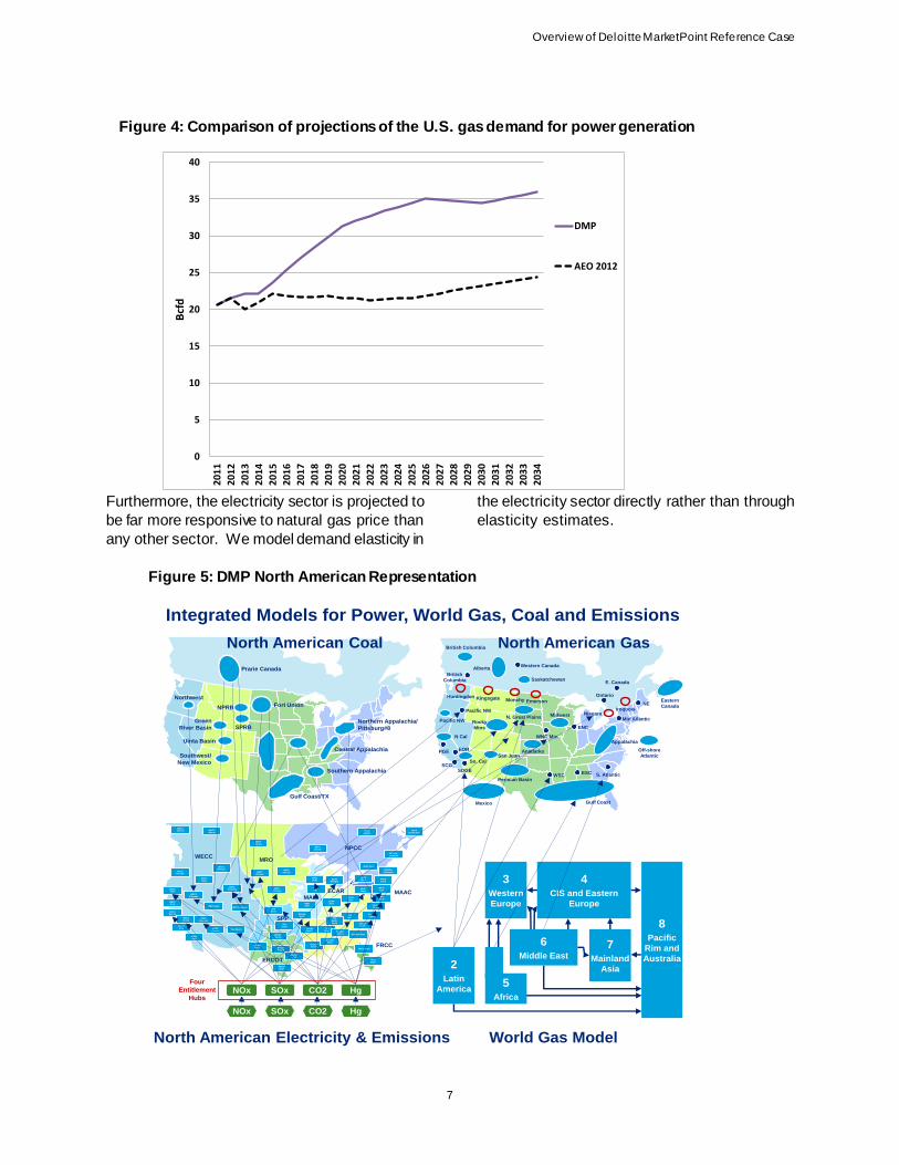
As shown in Figure 4, the DMP projected gas

demand for U.S. power generation gas is far

greater than the demand predicted by EIA’s

AEO 2012, which forecasts fairly flat demand for

power generation. In the U.S., the power sector,

which accounts for nearly all of the projected

future growth, is projected to increase by about

50% (approximately 11 Bcfd) over the next

decade. Our integrated electricity model projects

that natural gas will become the fuel of choice

for power generation due to a variety of reasons,

including: tightening application of existing

3 Approximately the average consumer price index over the

past 5 years according to the Bureau of Labor Statistics.

environmental regulations for mercury, NOx, and

SOx; expectations of ample domestic gas supply

at competitive gas prices; coal plant retirements;

and the need to back up intermittent renewable

sources such as wind and solar to ensure

reliability. Like the EIA’s AEO 2012 forecast, our

Reference Case projection does not assume any

new carbon legislation.

Our electricity model, fully integrated with our

gas (WGM) and coal models, contains a detailed

representation of the North American electricity

system including environmental emissions for

key pollutants (CO2, SOx, NOx, and mercury).

The integrated structure of these models is

shown in Figure 5. The electricity model projects

electric generation capacity addition, dispatch

and fuel burn based on competition among

different types of power generators given a

number of factors, including plant capacities, fuel

prices, heat rates, variable costs, and

environmental emissions costs. The model

integration of North American natural gas with

the rest of the world and the North American

electricity market captures the global linkages

and also the inter-commodity linkages.

Integrating gas and electricity is vitally important

because U.S. natural gas demand growth is

expected to be driven almost entirely by the

electricity sector, which is predicted to grow at

substantial rates.


7

Furthermore, the electricity sector is projected to

be far more responsive to natural gas price than

any other sector. We model demand elasticity in

the electricity sector directly rather than through

elasticity estimates.

Figure 4: Comparison of projections of the U.S. gas demand for power generation

0

5

10

15

20

25

30

35

40

20

11

20

12

20

13

20

14

20

15

20

16

20

17

20

18

20

19

20

20

20

21

20

22

20

23

20

24

20

25

20

26

20

27

20

28

20

29

20

30

20

31

20

32

20

33

20

34

Bcf

d

DMP

AEO 2012

Figure 5: DMP North American Representation

Northwest

Green

River Basin

Uinta Basin

Southwest/

New Mexico

Northern Appalachia/

Pittsburg#8

Central Appalachia

Southern Appalachia

Gulf Coast/TX

Prarie Canada

NPRB Fort Union

SPRB

WECC

Brit Col WECC

Alberta

WECC

Pac NW

WECC

Montana

MAPP

Canada

WECC

Idaho

WECC

COB

WECC

N Nevada

WECC

N CA

WECC

Bay CA

WECC

Ctrl CA

WECC

S CA

WECC

S Nevada

WECC

CMB

WECC

ArizonaNew Mexico

WECC ColoradoWECC Utah

WECC

Wyoming

MAPP

US-West

MAPP

US-East

MAPP

US-South

SPP

North

SPP

South

ERCOT

Nortla

ERCOT

West ERCOT

Central

ERCOT

Gulf

ERCOT

South

NPCC

Quebec

NPCC

Ontario

MAIN

WUMECAR

Michigan

MAIN

SOM

Entergy

North

ECAR

West

ECAR

East

Entergy

Central

TVA

West

TVA

East

MAAC

West

NVPP

West

Entergy

South

Southern

West

Southern

Central

NEPCOL

Northeast

NVPP North

NEPOOL

Southwest

NVPP

South

MAAC

East

MAAC

South

VACAR

North

VACAR

Central

VACAR

South

Southern East

FRCC North

FRCC

South

NPCC

Canada East

TVA

North/

South

WECCMRO

NPCC

MAAC

FRCC

MAIN

SPP

ERCOT

ECARMAIN

NIL

British Columbia

British

Columbia

Huntingdon

Pacific NW

N Cal

PGE EOR

SCGSDGE

So. CalSan Juan

Mexico

Kingsgate

AlbertaWestern Canada

Saskatchewan

Monchy Emerson

Rocky

Mtns

N. Great Plains

WNC Mtn

Anadarko

Permian BasinWSC

Midwest

ENC

ESC

Gulf Coast

Ontario

Niagara

E. Canada

Iroquois

Mid Atlantic

Appalachia

S. Atlantic

Off-shore

Atlantic

Eastern

CanadaPacific NW

NE

3Western

Europe

4CIS and Eastern

Europe

8Pacific

Rim and

Australia2

Latin

America5

Africa

6Middle East

7Mainland

Asia

NOx SOx CO2 Hg

NOx SOx CO2 Hg

Four

Entitlement

Hubs

North American Coal

North American Electricity & Emissions World Gas Model

North American Gas

Integrated Models for Power, World Gas, Coal and Emissions


8

Hence, the WGM projections include the impact

of increased natural gas demand for electricity

generation, which vies with LNG exports for

domestic supplies. From the demand

perspective, this is a conservative case in that

the WGM would project a larger impact of LNG

export than if we had assumed a lower US gas

demand, which would likely make more supply

available for LNG export and tend to lessen the

price impact. Higher gas demand would tend to

increase the projected prices impacts of LNG

export. However, the real issue is not the

absolute price of exported gas, but rather the

price impact resulting from the LNG exports.

The absolute price of natural gas will be

determined by a number of supply and demand

factors in addition to the volume of LNG exports.

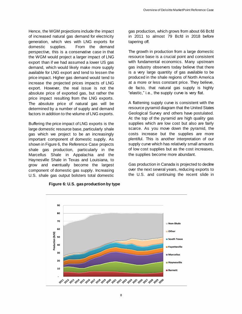
Buffering the price impact of LNG exports is the

large domestic resource base, particularly shale

gas which we project to be an increasingly

important component of domestic supply. As

shown in Figure 6, the Reference Case projects

shale gas production, particularly in the

Marcellus Shale in Appalachia and the

Haynesville Shale in Texas and Louisiana, to

grow and eventually become the largest

component of domestic gas supply. Increasing

U.S. shale gas output bolsters total domestic

gas production, which grows from about 66 Bcfd

in 2011 to almost 79 Bcfd in 2018 before

tapering off.

The growth in production from a large domestic

resource base is a crucial point and consistent

with fundamental economics. Many upstream

gas industry observers today believe that there

is a very large quantity of gas available to be

produced in the shale regions of North America

at a more or less constant price. They believe,

de facto, that natural gas supply is highly

“elastic,” i.e., the supply curve is very flat.

A flattening supply curve is consistent with the

resource pyramid diagram that the United States

Geological Survey and others have postulated.

At the top of the pyramid are high quality gas

supplies which are low cost but also are fairly

scarce. As you move down the pyramid, the

costs increase but the supplies are more

plentiful. This is another interpretation of our

supply curve which has relatively small amounts

of low cost supplies but as the cost increases,

the supplies become more abundant.

Gas production in Canada is projected to decline

over the next several years, reducing exports to

the U.S. and continuing the recent slide in

Figure 6: U.S. gas production by type


9

production out of the Western Canadian

Sedimentary Basin. However, Canadian

production is projected to ramp up in the later

part of this decade with increased production out

of the Horn River and Montney shale gas plays

in Western Canada. Further into the future, the

Mackenzie Delta pipeline may begin making

available supplies from Northern Canada.

Increased Canadian production makes more gas

available for export to the U.S.

Rather than basing our production projections

solely on the physical decline rates of producing

fields, the WGM considers economic

displacement as new, lower cost supplies force

their way into the market. The North American

natural gas system is highly integrated so

Canadian supplies can easily access U.S.

markets when economic.

Increasing production from major shale gas

plays, many of which are not located in

traditional gas-producing areas, has already

started to transform historical basis relationships

(the difference in prices between two markets)

and the trend is projected to continue during the

next two decades. Varying rates of regional gas

demand growth, the advent of new natural gas

infrastructure, and evolving gas flows may also

contribute to changes in regional basis, although

to a lesser degree.

Most notably, gas prices in the Eastern U.S.,

historically the highest priced region in North

America, could be dampened by incremental

shale gas production within the region. Eastern

bases to Henry Hub are projected to sink under

the weight of surging gas production from the

Marcellus Shale. Indeed, the flattening of

Eastern bases is already becoming evident. The

Marcellus Shale is projected to dominate the

Mid-Atlantic natural gas market, including New

York, New Jersey, and Pennsylvania, meeting

most of the regional demand and pushing gas

through to New England and even to South

Atlantic markets. Gas production from Marcellus

Shale will help shield the Mid-Atlantic region

from supply and demand changes in the Gulf

region. Pipelines built to transport gas supplies

from distant producing regions — such as the

Rockies and the Gulf Coast — to Northeastern

U.S. gas markets may face stiff competition. The

result could be displacement of volumes from

the Gulf which would depress prices in the Gulf

region. Combined with the growing shale

production out of Haynesville and Eagle Ford,

the Gulf region is projected to continue to have

plentiful production and remain one of the lowest

cost regions in North America.

Understanding the dynamic nature of the natural

gas market is paramount to understanding the

impact of LNG exports. If LNG is exported from

any particular location, the entire North

American natural gas system will potentially

reorient production, affecting basis differentials

and flows. Basis differentials are not fixed and

invariant to LNG exports or any other supply and

demand changes. On the contrary, LNG exports

will likely alter basis differentials, which lead to

redirection of gas flows to highest value markets

from each source given available capacity.

Potential impact of LNG exports

10


Impact on natural gas prices

We analyzed five LNG export cases within this

report: one case with Lavaca Bay only (1.33

Bcfd) and four other cases with varying levels of

total U.S. LNG export volumes (3 Bcfd, 6 Bcfd, 9

Bcfd and 12 Bcfd exports). Each case was run

with the DMP’s Integrated North American

Power and Gas Models in order to capture the

dynamic interactions across commodities.

For ease of reporting, we will focus on the

results with 6 Bcfd of LNG exports, our middle

case, without any implication that it is more likely

than any other case. Given the model’s

assumptions, the WGM projects 6 Bcfd of LNG

exports will result in a weighted-average price

impact of $0.15/MMBtu on the average U.S.

citygate price from 2018 to 2037. The

$0.15/MMBtu increase represents a 2.2%

increase in the projected average U.S. citygate

gas price of $6.96/MMBtu over this time period.

The projected increase in Henry Hub gas price is

$0.26/MMBtu during this period. It is important to

note the variation in price impact by location.

The impact at the Henry Hub will be much

greater than the impact in other markets more

distant from export terminals.

For all five export cases considered, the

projected natural gas price impacts at the Henry

Hub, New York, and average US citygate from

2018 through 2037 are shown in Figure 7.

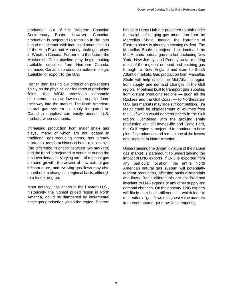
To put the impact in perspective, Figure 8 shows

the price impact of the midpoint 6 Bcfd case

compared to projected Reference Case U.S.

average citygate prices over a twenty year

period. The height of the bars represents the

projected price with LNG exports.

The small incremental price impact may not

appear intuitive or expected to those familiar

with market traded fluctuations in natural gas

prices. For example, even a 1 Bcfd increase in

demand due to sudden weather changes can

cause near term traded gas prices to surge

because in the short term, both supply and

demand are highly inelastic (i.e., fixed

quantities). However, in the long-term,

producers can develop more reserves in

anticipation of demand growth, e.g. due to LNG

exports. Indeed, LNG export projects will likely

be linked in the origination market to long-term

supply contracts, as well as long-term contracts

with LNG buyers. There will be ample notice and

Figure 7: Price impact by scenario for 2018-37 ($/MMBtu)

Export Case Average US

Citygate Henry Hub New York

1.33 Bcfd $ 0.03 $ 0.03 $ 0.02

3 Bcfd $ 0.07 $ 0.11 $ 0.06

6 Bcfd $ 0.15 $ 0.26 $ 0.14

9 Bcfd $ 0.22 $ 0.36 $ 0.23

12 Bcfd $ 0.30 $ 0.50 $ 0.29


11

time in advance of the LNG exports for suppliers

to be able to develop supplies so that they are

available by the time export terminals come into

operation. Therefore, under our long-term

equilibrium modeling assumptions, long-term

changes to demand may be anticipated and

incorporated into supply decisions. The built-in

market expectations allows for projected prices

to come into equilibrium smoothly over time.

Hence, our projected price impact primarily

reflects the estimated change in the production

cost of the marginal gas producing field with the

assumed export volumes.

As previously stated, the model projected price

impact varies by location as shown in Figure 9.

As previously described, the price impact

diminishes with distance from export terminals.

For all cases the impact is greatest at Henry

Hub, situated near most export terminals. For

the midpoint case of 6 Bcfd, the impact at the

Houston Ship Channel is nearly as much as

Henry Hub, at $0.26/MMBtu on average from

2018 to 2037. As distance from export terminals

increases (i.e., distance to downstream markets

such as Chicago, California and New York) the

price impact is generally only about $0.12 to

$0.14/MMBtu on average from 2018 to 2037.

Similarly, Figures 8 and 9 corresponding to the

other export cases (1.33, 3.0, 9.0 and 12.0 Bcfd)

are shown in the Appendix.

Figure 8: Projected Impact of LNG exports on average U.S. Citygate gas prices (Real 2012 $)


12

Impact on electricity prices

The projected impact on electricity prices is even

smaller than the projected impact on gas prices.

DMP’s integrated power and gas model allows

us to estimate incremental impact on electricity

prices resulting from LNG export assumptions,

as natural gas is also a fuel used for generating

electricity. Since our integrated model

represents the geographic linkages between the

electricity and natural gas systems, we can

compute the potential impact of LNG exports in

local markets (local to LNG exports) where the

impact would be the largest.

A similar comparison for electricity shows that

the projected average (2018-2037) electricity

prices increase by 0.8% in ERCOT (the Electric

Reliability Council of Texas), under the 6 Bcfd

export case. The impact on electricity prices is

much less than the 4.0% Henry Hub gas price

impact. For power markets in other regions, the

electricity price impact is much lower, because

the gas price impact is much lower.

A key reason why the price impact for electricity

is less than that of gas is that electricity prices

will only be directly affected by an increase in

gas prices when gas-fired generation is the

marginal source of power generation. That is,

gas price only affects power price if it changes

the marginal unit (i.e., the last unit in the

generation stack needed to service the final

amount of electricity load). When gas-fired

generation is lower cost than the marginal

source, then a small increase in gas price will

only impact electricity price if it is sufficient to

drive gas-fired generation to be the marginal

source of generation. If gas-fired generation is

already more expensive than the marginal

source of generation, then an increase in gas

price will not impact electricity price, since gas-

fired generation is not being utilized because

there is sufficient capacity from units with lower

generation costs.

If gas-fired generation is the marginal source,

then electricity price will increase with gas price,

but only up to the point that some other source

can displace it as marginal source. Every power

region has numerous competing power

generation plants burning different fuel types,

Figure 9: Price impact varies by location in 6 Bcfd export case (average 2018-37)


13

which will mitigate the price impact of an

increase in any one fuel type. Moreover, within

DPM’s integrated power and gas model, fuel

switching among coal, nuclear, gas, hydro, wind

and oil units is directly represented as part of the

modeling.

Figure 10 shows the power supply curve for

ERCOT. The curve plots the variable cost of

generation and capacity by fuel type. Depending

on where the demand curve intersects the

supply curve, a generating unit with a particular

fuel type will set the electricity price. During

extremely low demand periods, hydro, nuclear or

coal plants will likely set the price. An increase in

gas price during these periods would not impact

electricity price in this region because gas-fired

plants are typically not utilized. Since the

marginal source sets the price, a change in gas

price under these conditions would not affect

power prices.

Figure 10: Power supply curve for ERCOT region


14

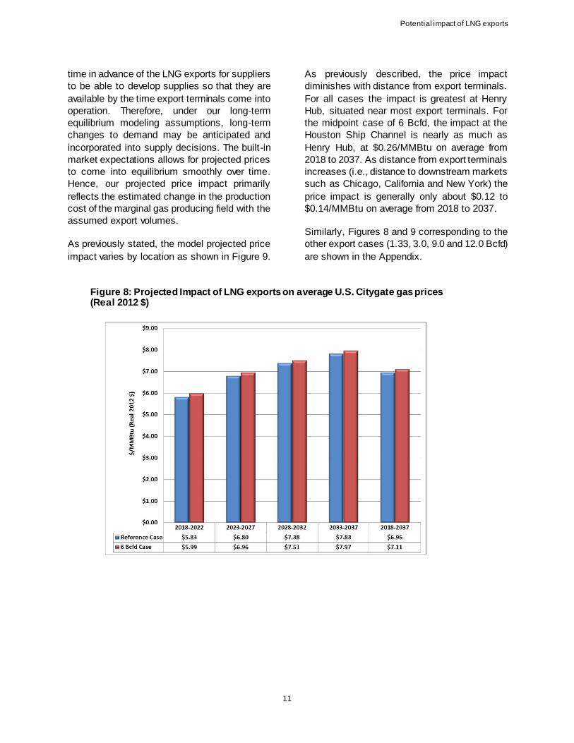
Incremental production impact in Texas from Lavaca Bay export

All of the gas used as feedstock for 1.33 Bcfd of

LNG exports from Lavaca Bay is projected to

come from Texas production. About one-third of

the gas is incremental supplies from Texas

production with the remaining two-thirds coming

from Texas gas that would have otherwise been

exported out of the state but instead is diverted

to the terminal. The diverted volumes stimulate

production in other supply basins outside Texas.

Figure 11 shows the projected increase in

production volume on average from 2018-2037.

The shale gas basins that are entirely or at least

partially located in Texas are separated to

highlight the impact on the State. One might

expect South Texas, which includes Eagle Ford

shales, to have a larger incremental impact.

However, the region is rich in liquids and is

projected to grow strongly even without boost

from LNG exports. The incremental supplies

indicate the marginal regions which would be

stimulated with incremental demand.

Barnett, 105

South Texas, 89

Haynesville, 149

Marcellus, 123

Fayetteville, 21

Other Shale Gas, 180

Non-Shale, 188

Figure 11: Average incremental production with Lavaca Bay export, 2018-37 (MMcfd)


15

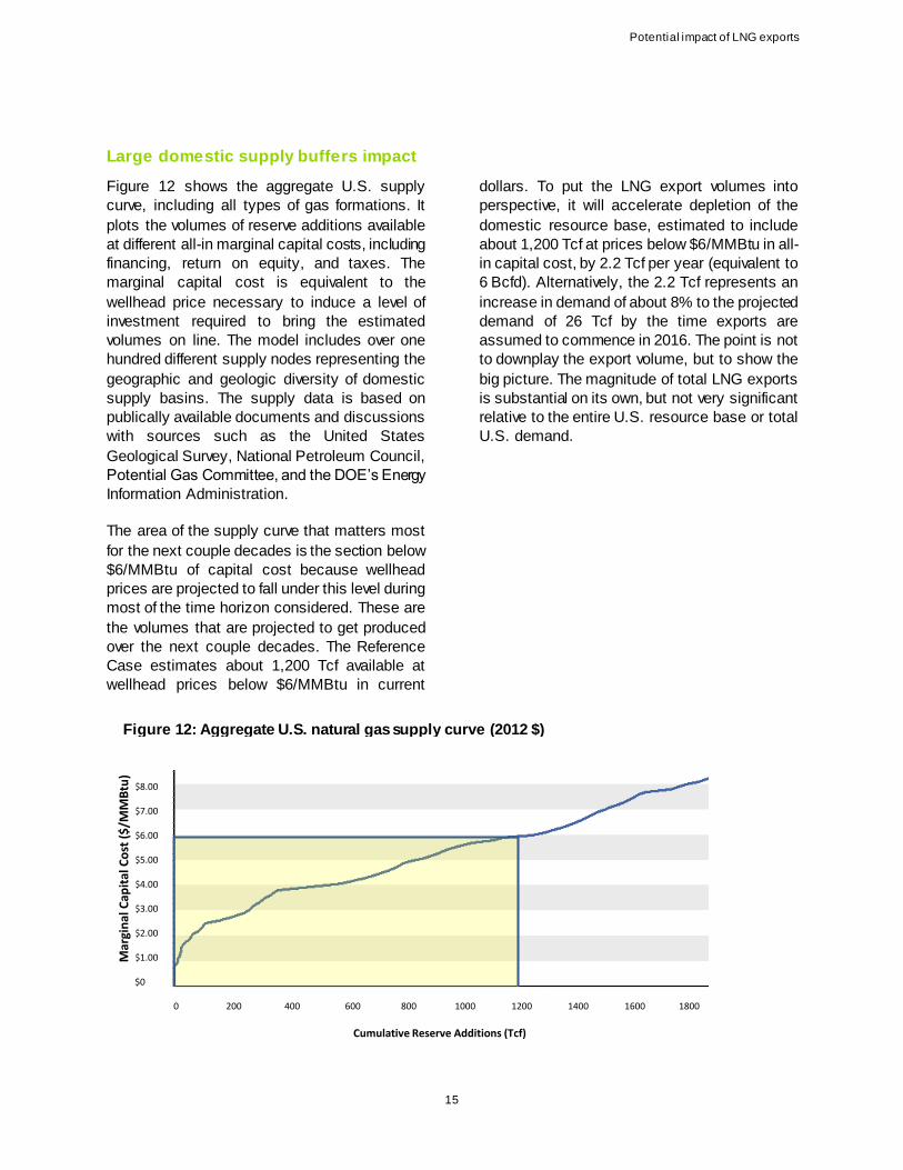
Large domestic supply buffers impact

Figure 12 shows the aggregate U.S. supply

curve, including all types of gas formations. It

plots the volumes of reserve additions available

at different all-in marginal capital costs, including

financing, return on equity, and taxes. The

marginal capital cost is equivalent to the

wellhead price necessary to induce a level of

investment required to bring the estimated

volumes on line. The model includes over one

hundred different supply nodes representing the

geographic and geologic diversity of domestic

supply basins. The supply data is based on

publically available documents and discussions

with sources such as the United States

Geological Survey, National Petroleum Council,

Potential Gas Committee, and the DOE’s Energy

Information Administration.

The area of the supply curve that matters most

for the next couple decades is the section below

$6/MMBtu of capital cost because wellhead

prices are projected to fall under this level during

most of the time horizon considered. These are

the volumes that are projected to get produced

over the next couple decades. The Reference

Case estimates about 1,200 Tcf available at

wellhead prices below $6/MMBtu in current

dollars. To put the LNG export volumes into

perspective, it will accelerate depletion of the

domestic resource base, estimated to include

about 1,200 Tcf at prices below $6/MMBtu in all-

in capital cost, by 2.2 Tcf per year (equivalent to

6 Bcfd). Alternatively, the 2.2 Tcf represents an

increase in demand of about 8% to the projected

demand of 26 Tcf by the time exports are

assumed to commence in 2016. The point is not

to downplay the export volume, but to show the

big picture. The magnitude of total LNG exports

is substantial on its own, but not very significant

relative to the entire U.S. resource base or total

U.S. demand.

Figure 12: Aggregate U.S. natural gas supply curve (2012 $)

Cumulative Reserve Additions0 200 400 600 800 1000 1200 1400 1600 1800

Cumulative Reserve Additions (Tcf)

$8.00

$7.00

$6.00

$5.00

$4.00

$3.00

$2.00

$1.00

$0

Mar

gin

al C

apit

al C

ost

($

/MM

Btu

)


16

With regards to the potential impact of LNG

exports, the absolute price is not the driving

factor but rather the shape of the aggregate

supply curve which determines the price impact.

Figure 13 depicts how demand increase affects

price. Incremental demand pushes out the

demand curve, causing it to intersect the supply

curve at a higher point. Since the supply curve is

fairly flat in the area of demand, the price impact

is fairly small. The massive shale gas resources

have flattened the U.S. supply curve. It is the

shape of the aggregate supply curve that really

matters. Hence, leftward and rightward

movements in the demand curve (where such

leftward and rightward movements would be

volumes of LNG export) cut through the supply

curve at pretty much the same price. Flat, elastic

supply means that the price of domestic natural

gas is increasingly and continually determined

by supply issues (e.g., production cost). Given

that there is a significant quantity of domestic

gas available at modest production costs, the

export of 6 Bcfd of LNG would not increase the

price of domestic gas very much because it

would not increase the production cost of

domestic gas very much.

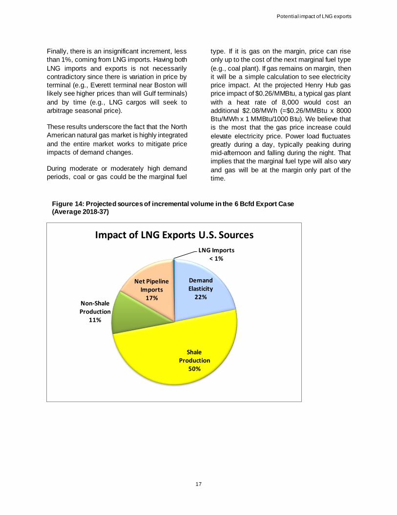
The projected sources of incremental volumes

used to meet the assumed export volumes come

from multiple sources, including domestic

resources (both shale gas and non-shale gas),

import volumes, and demand elasticity. Figure

14 shows the sources of incremental volumes in

the 6 Bcfd LNG export case on average from

2018 to 2037, the assumed years of LNG

exports. (The source fractions are similar for

other LNG export cases so we only show the 6

Bcfd case.) The bulk of the incremental volumes

come from shale gas production. Including non-

shale gas production, the domestic production

contributes 63% of the total incremental volume.

Net pipeline imports, comprised mostly of

imports from Canada, contribute another 18%.

Higher U.S. prices induce greater Canadian

production, primarily from Horn River and

Montney shale gas resources, making gas

available for export to the U.S. The net exports

to Mexico declines slightly as higher cost of U.S.

supplies will likely prompt more Mexican

production and would reduce the need for U.S.

exports to Mexico. Higher gas prices are also

projected to trigger demand elasticity so less gas

is consumed, representing about 19% of the

incremental volume. Most of the reduction in gas

consumption comes from the power sector as

higher gas prices incentivize greater utilization of

generators burning other types of fuels.

Figure 13: Impact of higher demand on price (illustrative)

Cumulative Reserve Additions

Increased Demand

Price Impact

0 200 400 600 800 1000 1200 1400 1600 1800

Cumulative Reserve Additions (Tcf)

$8.00

$7.00

$6.00

$5.00

$4.00

$3.00

$2.00

$1.00

$0

Mar

gin

al C

apit

al C

ost

($

/MM

Btu

)


17

Finally, there is an insignificant increment, less

than 1%, coming from LNG imports. Having both

LNG imports and exports is not necessarily

contradictory since there is variation in price by

terminal (e.g., Everett terminal near Boston will

likely see higher prices than will Gulf terminals)

and by time (e.g., LNG cargos will seek to

arbitrage seasonal price).

These results underscore the fact that the North

American natural gas market is highly integrated

and the entire market works to mitigate price

impacts of demand changes.

During moderate or moderately high demand

periods, coal or gas could be the marginal fuel

type. If it is gas on the margin, price can rise

only up to the cost of the next marginal fuel type

(e.g., coal plant). If gas remains on margin, then

it will be a simple calculation to see electricity

price impact. At the projected Henry Hub gas

price impact of $0.26/MMBtu, a typical gas plant

with a heat rate of 8,000 would cost an

additional $2.08/MWh (=$0.26/MMBtu x 8000

Btu/MWh x 1 MMBtu/1000 Btu). We believe that

is the most that the gas price increase could

elevate electricity price. Power load fluctuates

greatly during a day, typically peaking during

mid-afternoon and falling during the night. That

implies that the marginal fuel type will also vary

and gas will be at the margin only part of the

time.

Demand Elasticity

22%

Shale Production

50%

Non-Shale Production

11%

Net Pipeline Imports

17%

LNG Imports < 1%

Impact of LNG Exports U.S. Sources

Figure 14: Projected sources of incremental volume in the 6 Bcfd Export Case (Average 2018-37)

Comparison of results to other studies

18


A number of studies, including others submitted

to the DOE in association with LNG export

applications, have estimated impacts of LNG

exports from the U.S. The EIA also performed a

study4 at the request of the DOE. The various

studies used different models and assumptions,

but a comparison of their results might shed

some light on the key factors and range of

possible outcomes.

Figure 15 compares projections of estimated

Henry Hub price impact from 2015 to 2035 with

6 Bcfd of LNG exports. The price impact ranges

from 4% to 11%, with this study being on the low

end and the ICF International being on the high

end. The first observation is that, although the

percentage differences are large on a relative

basis, the range of estimated impacts is not so

large. These studies consistently show that the

price impact will not be that large relative to the

change in demand. Bear in mind that 6 Bcfd is a

fairly large incremental demand. In fact, it

exceeds the combined gas demands in New

4 “Effect of Increased Natural Gas Exports on Domestic

Energy Markets,” Howard Gruenspecht, EIA, January 2012.

York (3.3 Bcfd) and Pennsylvania (2.4 Bcfd) in

2011. These studies indicate that adding a

sizeable incremental gas load on the U.S.

energy system might result in a gas price

increase of 11% or less.

Although we have limited data relating to specific

assumptions and detailed output from the other

studies, we can infer why the impacts differ so

much. By most accounts, the resource base in

the United States is plentiful, perhaps sufficient

to last some 100 years at current production

levels. All of the studies listed, including our

own, had estimated natural gas resource

volumes, including proved reserves and

undiscovered gas of all types, of over 2,000 Tcf.

Why then would the LNG export impacts vary as

much as they do?

An important distinction between our analysis

and the other studies is the representation of

market dynamics, particularly for supply

response to demand changes. That is, how do

the studies represent how producers will

respond to demand changes? The World Gas

Model has a dynamic supply representation in

which producers are assumed to anticipate

demand and price changes. Producers do more

than just respond to price that they see, but

Figure 15: Comparison of projected price impact from 2015-35 at the Henry Hub with 6 Bcfd of LNG exports

Study

Price without

Exports ($/MMBtu)

Price with Exports

($/MMBtu)

Average Price

Increase (%)

EIA 5.28$ 5.78$ 9%

Navigant (2010) 4.75$ 5.10$ 7%

Navigant (2012) 5.67$ 6.01$ 6%

ICF International 5.81$ 6.45$ 11%

Deloitte MarketPoint 6.11$ 6.37$ 4%

Source: Brookings Institute for all estimates besides Deloitte MarketPoint’s


19

rather anticipate events. Accordingly, prices will

rise to induce producers to develop supplies in

time to meet future demand.

Other models, primarily based on linear

programming (LP)5 or similar approaches, use

static representation of supply in that supply

does not anticipate price or demand growth.

These static supply models require the user to

input estimates of productive capacities in each

future time period. The Brookings Institution

completed a study assessing the impact of LNG

exports and analyzing different economic

approaches.6 . As the Brookings study states:

“… static supply model, which, unlike dynamic

supply models, does not fully take account of the

effect that higher prices have on spurring

additional production.”

Since the supply volumes available in each time

period is an input into LP models, the user must

input how supply will respond to demand. In the

case of LNG exports, the user must input how

much supplies will increase and how quickly

given the export volumes. Hence, the price

impact is largely determined by how the user

changes these inputs.

The purpose of this discussion is not to assert

which approach is best, but rather to understand

the differences so that the projections can be

understood in their proper context. Assuming

little or no price anticipation will tend to elevate

the projected price impact while assuming price

anticipation will tend to mitigate the projected

price impact. Depending on the issue being

analyzed, one approach may be more

5 Linear programming (“LP”) is a mathematical technique for

solving a global objective function subject to a series of

l inear constraints

6 “Liquid Markets: Assessing the Case for U.S. Exports of

Liquefied Natural Gas,” Brookings Institution (2012).

appropriate than the other. In the case of LNG

export terminals, our belief is that the

assumption of dynamic supply demand balance

is appropriate. Given the long lead time,

expected to be at least five years, required to

permit, site, and construct an LNG export

terminal, producers will have both ample time

and plenty of notice to prepare for the export

volumes. It would be a different matter if exports

were to begin with little advanced notice.

The importance of timing is evident in EIA’s

projections. The projected price impact is highly

dependent on how quickly export volumes are

assumed to ramp up. Furthermore, in all cases,

the impacts are the greatest in the early years of

exports. The impacts dissipate over time as

supplies are assumed to eventually catch up

with the demand growth.

Natural gas producers are highly sophisticated

companies with analytical teams monitoring and

forecasting market conditions. Producers, well

aware of the potential LNG export projects, are

looking forward to the opportunity to supply

these projects.

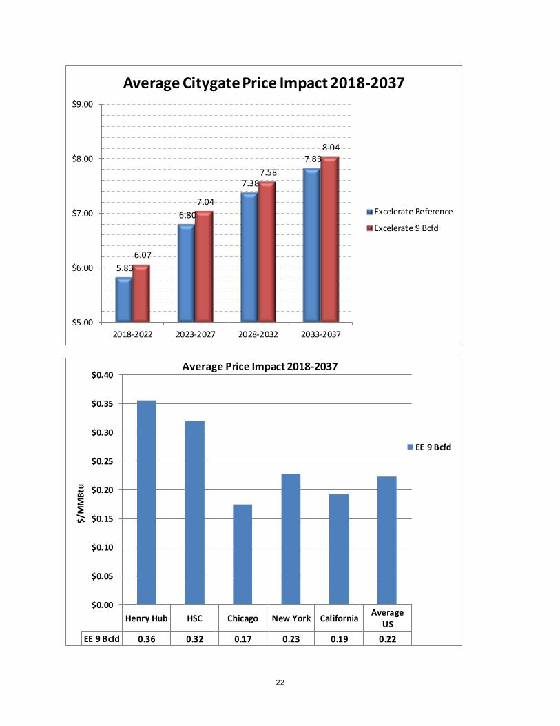
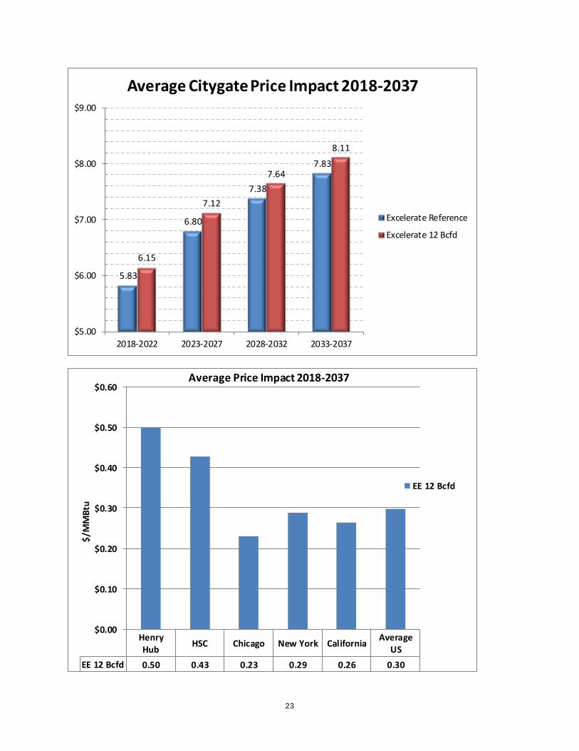
20

Appendix A: Price Impact Charts for other Export Cases

5.83

6.80

7.38

7.83

5.85

6.83

7.41

7.85

$5.00

$6.00

$7.00

$8.00

2018-2022 2023-2027 2028-2032 2033-2037

Average Citygate Price Impact 2018-2037

Excelerate Reference

Excelerate Lavaca Bay

Henry Hub HSC Chicago New York California Average US

EE Lavaca Bay 0.03 0.06 0.02 0.02 0.03 0.03

$0.00

$0.01

$0.02

$0.03

$0.04

$0.05

$0.06

$0.07

$/M

MB

tu

Average Price Impact 2018-2037

EE Lavaca Bay

21

5.83

6.80

7.38

7.83

5.90

6.88

7.44

7.89

$5.00

$6.00

$7.00

$8.00

$9.00

2018-2022 2023-2027 2028-2032 2033-2037



Excelerate 3 Bcfd

Henry Hub HSC Chicago New York California Average US

EE 3 Bcfd 0.11 0.09 0.06 0.06 0.06 0.07

$0.00

$0.02

$0.04

$0.06

$0.08

$0.10

$0.12

$/M

MB

tu


EE 3 Bcfd

22

5.83

6.80

7.38

7.83

6.07

7.04

7.58

8.04

$5.00

$6.00

$7.00

$8.00

$9.00

2018-2022 2023-2027 2028-2032 2033-2037



Excelerate 9 Bcfd

Henry Hub HSC Chicago New York CaliforniaAverage

US

EE 9 Bcfd 0.36 0.32 0.17 0.23 0.19 0.22

$0.00

$0.05

$0.10

$0.15

$0.20

$0.25

$0.30

$0.35

$0.40

$/M

MB

tu


EE 9 Bcfd

23

5.83

6.80

7.38

7.83

6.15

7.12

7.64

8.11

$5.00

$6.00

$7.00

$8.00

$9.00

2018-2022 2023-2027 2028-2032 2033-2037



Excelerate 12 Bcfd

HenryHub

HSC Chicago New York CaliforniaAverage

US

EE 12 Bcfd 0.50 0.43 0.23 0.29 0.26 0.30

$0.00

$0.10

$0.20

$0.30

$0.40

$0.50

$0.60

$/M

MB

tu


EE 12 Bcfd

24

Appendix B: DMP’s World Gas Model and data

To help understand the complexities and

dynamics of global natural gas markets, DMP

uses its World Gas Model (“WGM”) developed in

our proprietary MarketBuilder software. The

WGM, based on sound economic theories and

detailed representations of global gas demand,

supply basins, and infrastructure, projects

market clearing prices and quantities over a long

time horizon on a monthly basis. The projections

are based on market fundamentals rather than

historical trends or statistical extrapolations.

WGM represents fundamental producer

decisions regarding the timing and quantity of

reserves to develop given the producer’s

resource endowments and anticipated forward

prices. This supply-demand dynamic is

particularly important in analyzing the market

value of gas supply in remote parts of the world.

The WGM uses sophisticated depletable

resource logic in which today’s drilling decisions

affect tomorrow’s price and tomorrow’s price

affects today’s drilling decisions. It captures the

market dynamics between suppliers and

consumers.

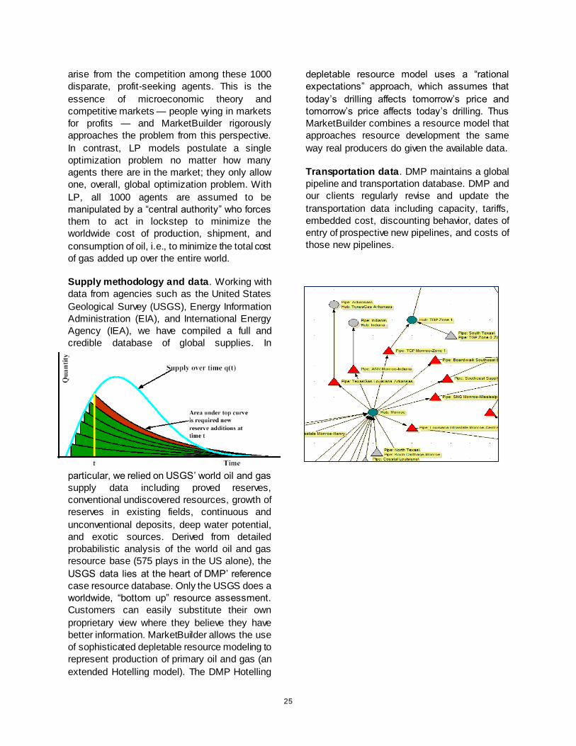
WGM simulates how regional interactions

among supply, transportation, and demand

interact to determine market clearing prices,

flowing volumes, reserve additions, and pipeline

entry and exit through 2046. The WGM divides

the world into major geographic regions that are

connected by marine freight. Within each major

region are very detailed representations of many

market elements: production, liquefaction,

transportation, market hubs, regasification and

demand by country or sub area. All known

significant existing and prospective trade routes,

LNG liquefaction plants, LNG regasification

plants and LNG terminals are represented.

Competition with oil and coal is modeled in each

region. The capability to model the related

markets for emission credits and how these may

impact LNG markets is included. The model

includes detailed representation of LNG

liquefaction, shipping, and regasification;

pipelines; supply basins; and demand by sector.

Each regional diagram describes how market

elements interact internally and with other

regions.

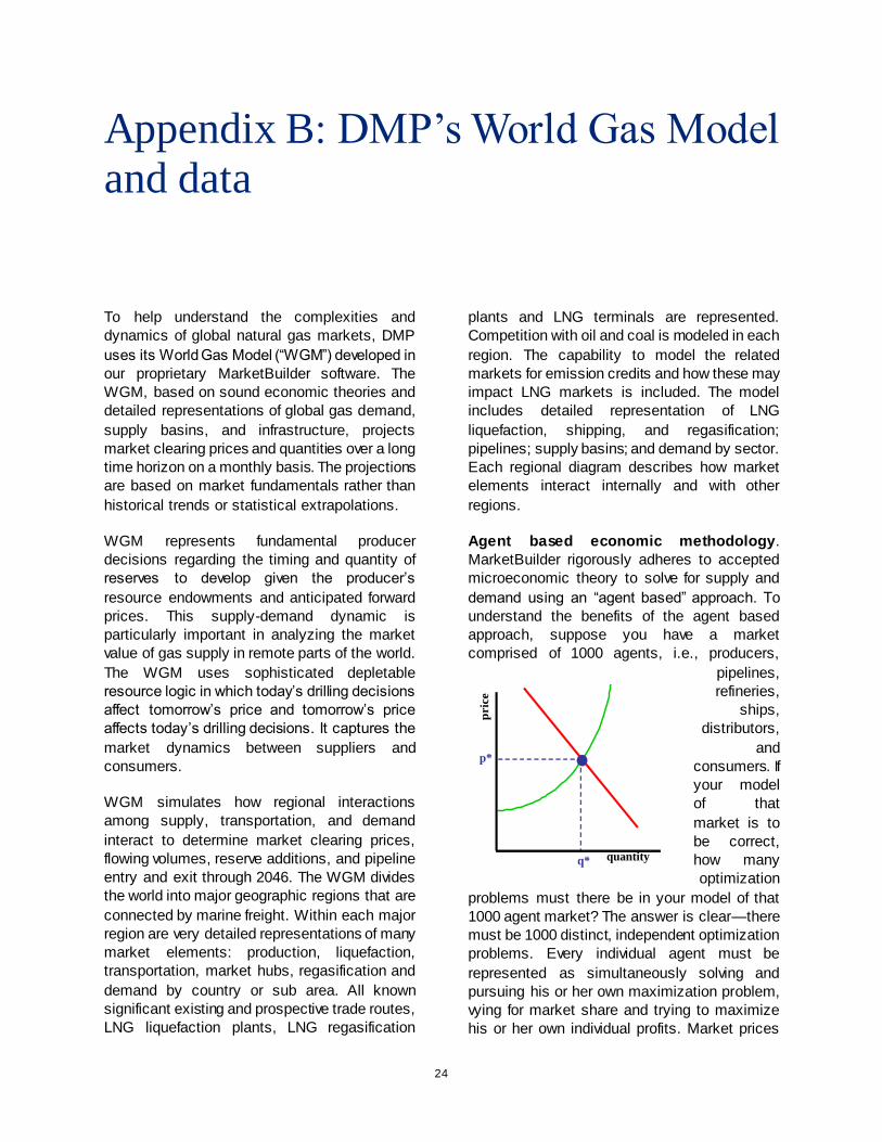
Agent based economic methodology.

MarketBuilder rigorously adheres to accepted

microeconomic theory to solve for supply and

demand using an “agent based” approach. To

understand the benefits of the agent based

approach, suppose you have a market

comprised of 1000 agents, i.e., producers,

pipelines,

refineries,

ships,

distributors,

and

consumers. If

your model

of that

market is to

be correct,

how many

optimization

problems must there be in your model of that

1000 agent market? The answer is clear—there

must be 1000 distinct, independent optimization

problems. Every individual agent must be

represented as simultaneously solving and

pursuing his or her own maximization problem,

vying for market share and trying to maximize

his or her own individual profits. Market prices

p*

q* quantity

pric

e

25

arise from the competition among these 1000

disparate, profit-seeking agents. This is the

essence of microeconomic theory and

competitive markets — people vying in markets

for profits — and MarketBuilder rigorously

approaches the problem from this perspective.

In contrast, LP models postulate a single

optimization problem no matter how many

agents there are in the market; they only allow

one, overall, global optimization problem. With

LP, all 1000 agents are assumed to be

manipulated by a “central authority” who forces

them to act in lockstep to minimize the

worldwide cost of production, shipment, and

consumption of oil, i.e., to minimize the total cost

of gas added up over the entire world.

Supply methodology and data. Working with

data from agencies such as the United States

Geological Survey (USGS), Energy Information

Administration (EIA), and International Energy

Agency (IEA), we have compiled a full and

credible database of global supplies. In

particular, we relied on USGS’ world oil and gas

supply data including proved reserves,

conventional undiscovered resources, growth of

reserves in existing fields, continuous and

unconventional deposits, deep water potential,

and exotic sources. Derived from detailed

probabilistic analysis of the world oil and gas

resource base (575 plays in the US alone), the

USGS data lies at the heart of DMP’ reference

case resource database. Only the USGS does a

worldwide, “bottom up” resource assessment.

Customers can easily substitute their own

proprietary view where they believe they have

better information. MarketBuilder allows the use

of sophisticated depletable resource modeling to

represent production of primary oil and gas (an

extended Hotelling model). The DMP Hotelling

depletable resource model uses a “rational

expectations” approach, which assumes that

today’s drilling affects tomorrow’s price and

tomorrow’s price affects today’s drilling. Thus

MarketBuilder combines a resource model that

approaches resource development the same

way real producers do given the available data.

Transportation data. DMP maintains a global

pipeline and transportation database. DMP and

our clients regularly revise and update the

transportation data including capacity, tariffs,

embedded cost, discounting behavior, dates of

entry of prospective new pipelines, and costs of

those new pipelines.

26

Non-linear demand methodology.

MarketBuilder allows the use of multi-variate

nonlinear representations of demand by sector,

without limit on the number of demand sectors.

DMP is skilled at performing regression analyses

on historical data to evaluate the effect of price,

weather, GNP, etc. on demand. Using our

methodology, DMP systematically models the

impact of price change on demand (demand

price feedback) to provide realistic results.

deloitte marketpoint. analysis of economic impact of lng

Documents