demand elasticity, risk classification and loss … · ticity in an insurance market where risk...

DEMAND ELASTICITY, RISK CLASSIFICATION AND LOSS COVERAGE:WHEN CAN COMMUNITY RATING WORK?

BY

R. GUY THOMAS

ABSTRACT

This paper investigates the effects of high or low fair-premium demand elas-ticity in an insurance market where risk classification is restricted. The effectsare represented by the equilibrium premium, and the risk-weighted insurancedemand or “loss coverage”. High fair-premium demand elasticity leads to acollapse in loss coverage, with an equilibrium premium close to the risk of thehigher-risk population. Low fair-premium demand elasticity leads to anequilibrium premium close to the risk of the lower-risk population, and highloss coverage – possibly higher than under more complete risk classification.The demand elasticity parameters which are required to generate a collapse incoverage in the model in this paper appear higher than the values for demandelasticity which have been estimated in several empirical studies of variousinsurance markets. This offers a possible explanation of why some insurancemarkets appear to operate reasonably well under community rating, withoutthe collapse in coverage which insurance folklore suggests.

KEYWORDS

Adverse selection, loss coverage, risk classification, demand elasticity, com-munity rating.

1. INTRODUCTION

Conventional wisdom or “insurance folklore” suggests that the absence of riskclassification in an insurance market is likely to lead to an adverse selectionspiral, which may progress until the market largely disappears. A succinct artic-ulation of this concept is provided by the policy document Insurance & Super-annuation Risk Classification Policy published by the Institute of Actuaries ofAustralia (IAA, 1994), which explains:

“In the absence of a system that allows for distinguishing by price betweenindividuals with different risk profiles, insurers would provide an insurance orannuity product at a subsidy to some while overcharging others. In an open

Astin Bulletin 39(2), 403-428. doi: 10.2143/AST.39.2.2044641 © 2009 by Astin Bulletin. All rights reserved.

market, basic economics dictates that individuals with low risk relative to pricewould conclude that the product is overpriced and thus reduce or possiblyforgo their insurance. Those individuals with a high level of risk relative toprice would view the price as attractive and therefore retain or increase theirinsurance. As a result the average cost of the insurance would increase, thuspushing prices up. Then, individuals with lower loss potential would continueto leave the marketplace, contributing to a further price spiral. Eventuallythe majority of consumers, or the majority of providers of insurance, wouldwithdraw from the marketplace and the remaining products would becomefinancially unsound”.

However, the concept that restrictions on risk classification lead inevitably tomarket collapse is difficult to reconcile with the operation of many extant insur-ance markets. In particular, there are various markets in which regulators imposesome restrictions on risk classification, or even mandate “community rating”,whereby little or no classification of risk is permitted. Examples of restrictionswhich stop short of pure community rating include the prohibition of ratingby gender, race or genetic test results in a number of insurance markets. Exam-ples of community rating in voluntary health insurance include schemes inIreland, Australia, Switzerland and South Africa, and US states including NewYork, New Jersey, and Vermont1. These schemes generally include some pro-vision for risk equalization payments between insurers, or stop-loss state rein-surance (but not always, and the relevant provisions are not always actuallyused). However the prevalence and persistence of various community ratingschemes or partial restrictions on rating factors does not seem consistent withthe notion that regulatory limitations on risk classification lead inevitably tomarket collapse.

This paper uses a simple model of an insurance market with two riskgroups, one lower-risk and one higher-risk. Insurance market outcomes in theabsence of risk classification are characterized by the pooled premium chargedto all policyholders, and the risk-weighted insurance demand or “loss cover-age”. It is shown that insurance market outcome in the absence of riskclassification depends on a parameter for the elasticity of demand for insur-ance at an actuarially fair premium, that is the “fair-premium demand elas-ticity”. High fair-premium demand elasticity leads to an equilibrium premiumclose to the risk of the higher-risk population, and a low loss coverage. Butfor sufficiently low fair-premium demand elasticity, this market collapse doesnot occur; instead, the market stabilizes with a relatively low premium, andrelatively high loss coverage – possibly higher than under more complete riskclassification. The ranges for the demand elasticity parameter characterizedas “high” and “low” are separated by a threshold range for the parameterwhich leads to an unstable market outcome – either multiple equilibria (that

404 R.G. THOMAS

1 A number of other US states apply varying degrees of restrictions on risk classification in healthinsurance, such as maximum premium relativities, or allowing some rating factors but not others.Gale (2007) gives further details.

is, more than one pooled premium is capable of equilibrating insurers’ revenueand claims), or near-equilibria for an extended range of premium values. Gen-erally, the threshold range of values for the demand elasticity parameter abovewhich a collapse in coverage occurs in the model in this paper appears higherthan the values for demand elasticity which have been estimated in empiricalstudies of various insurance markets. The high demand elasticity conditionswhich correspond to the threshold for a large fall in coverage in the model inthis paper may explain why some insurance markets appear to operate rea-sonably well under community rating, without the collapse in coverage whichinsurance folklore suggests.

A number of previous authors have suggested that insurance folklore accountsof adverse selection spirals might sometimes be overblown. Siegelman (2004)surveys the use of rhetoric about adverse selection in legal judgments andpublic policy advocacy, drawing a contrast with the limited and sometimescontradictory evidence from empirical studies. Buchmueller & DiNardio (2002)note that “Whilst the notion that community rating leads to adverse selectiondeath spirals appears to have passed into the “conventional wisdom”, at leastamongst industry analysts and policy experts, this is not a result which arisesnaturally from the simplest economic models of insurance”. These authorsfound no evidence for an adverse selection spiral after the State of New Yorkintroduced pure community rating for health insurance in 1993. From a prac-tical perspective, some actuaries may feel that their experience of communityrating is more negative. One careful study did report evidence of an adverseselection spiral in health insurance (Cutler & Reber, 1998)2; but their examplewas essentially a case of selection against one insurer amongst many in a sce-nario where different health insurance plans offered differing benefit structuresand premiums. However, this is not the same as the selection against the wholemarket which it is often said will lead to collapse of the market under manda-tory community rating. Intuitively, in the scenario of multiple health plans,the various choices are reasonably close substitutes, and so demand elasticityfor any one plan may be high; but in the scenario of mandatory community rat-ing, remaining uninsured is often not a close substitute for being insured, and sodemand elasticity for insurance from all providers could be lower. The model inthis paper allows the effects of different demand elasticities to be explored ingreater depth.

There are a number of approaches to modeling adverse selection in recentactuarial literature. One approach uses Markov models with an assumed highdegree of adverse selection, in the sense that a small proportion of the population

WHEN CAN COMMUNITY RATING WORK? 405

2 Cutler & Reber (1998) report that Harvard University offered employees a choice between differenthealth insurance plans with different benefits, originally with an employer contribution as a fixedpercentage of the premiums. The employer contribution was then changed to the same flat contribu-tion irrespective of which plan the employee chose. This led to a rapid migration of younger, healthieremployees from the more expensive plan with better benefits to the cheaper plan with lower benefits.The more expensive plan suffered reducing enrolments and progressively increasing per capita costs,leading to its withdrawal three years after the change in employer contributions.

acquires private information (eg a genetic test result) indicating much higherrisk, and this leads to much higher transition intensity into the insured state,or a tendency to buy much larger amounts of insurance; the effect of thisadverse selection is measured by the increase in the pooled insurance price,compared with the price if the private information did not exist. In thisapproach, it is sufficient to use exogenous and very high assumptions for thetransition intensities, because the rarity of the private information consideredmeans that even extreme assumptions lead to negligible increases in the pooledpremium (Macdonald, 1997, 1999, 2003). However if the private informationconsidered is more common and indicative of only moderately higher risk,extreme assumptions may be neither plausible nor sufficient. In these cir-cumstances a second approach is to postulate utility functions for insureds,and that adverse selection arises only if lower risks achieve lower expectedutility by insuring at the pooled price than by not insuring (Macdonald &Tapadar, 2007). A third approach is to model insurance demand from lowerand higher-risk groups as a function of the pooled price, with a demand elas-ticity parameter, and investigate insurance market outcome under differentdemand elasticities (De Jong & Ferris, 2006). The present paper follows thisthird approach.

Some previous economics literature has drawn attention to the possibilityof multiple equilibria in markets with adverse selection, in particular Wilson(1979, 1980). However these papers focus on the markets for goods of varyingquality – where the quality is known to sellers, but unobservable by buyers –rather than on insurance markets. Rose (1993) showed that although multipleequilibria in markets for goods of varying quality are theoretically possible, theyare extremely unlikely, provided that the quality distribution of the goods fol-lows any of a range of plausible probability distributions. The present paperprovides some insight into why multiple equilibria may also be unlikely,although not impossible, in models of insurance markets.

The rest of this paper is structured as follows. Section 2 outlines the insur-ance market model, and characterizes the possible equilibria according towhether loss coverage is higher or lower than under full risk classification.Section 3 investigates conditions for multiple equilibria in the model, consid-ering the relative sizes of the higher and lower-risk populations, their relativerisks, and demand elasticity. Conclusions are given in Section 4.

2. THE MODEL

We assume that potential insureds can in principle be divided into two groups,which we refer to as populations. Members of population 1 are lower-risk, andmembers of population 2 are higher-risk. We assume that regulation requiresall insurers to use community rating, that is a single common insurance pricemust apply irrespective of whether an individual risk belongs to the higher orlower-risk population; competition in risk classification of a “cream-skimming”

406 R.G. THOMAS

FIGURE 1: Insurance demand function for specimen values of fair-premium elasticity l.

nature is not possible. We also assume that the probability of a loss is inde-pendent of insurance purchase, that is moral hazard is ignored. Equilibriumin the insurance market occurs when total premiums equal total claims, thatis insurers make zero profits in equilibrium.

The demand for insurance from population i at a premium of p is specifiedalong the lines suggested by de Jong & Ferris (2006):

di(p) = Pi e1 – (p /mi)

lii = 1,2 (1)

where

– Pi is the number of members of the population of risk class i who buy insur-ance at an actuarially fair premium, that is when p = mi

– mi is the risk (expectation of claim) for population i

– li is an elasticity parameter for insurance demand of population i.

The specification of Pi as the number of members of population i who buyinsurance at an actuarially fair premium assumes that all insurance is for unitsum assured, that is every agent either buys one unit of insurance or none.This simplification is convenient for exposition, but it is not necessary: Pi couldalternatively be regarded as the fair-premium money demand for insurancefrom population i (as in de Jong & Ferris, 2006).

The formula can be interpreted as follows: when p is very small relative tomi demand from population i will be high. As the “premium loading” p /mi

increases, demand from population i declines along an inverse exponentialcurve towards zero; this reflects the fact that if the premium loading p /mi is highenough, almost no-one would buy insurance. This specification allows a rangeof plausible demand curves to be specified for the relevant range of m1 < p ≤ m2.This is illustrated in Figure 1.


The parameter li specifies the responsiveness of demand from population i tochanges in the premium p. The price elasticity of demand di with respect to pis defined as

i

i

ddp

pp

$2

2 ] g

where we have taken absolute values to obviate the usual negative sign of theelasticity. This is equivalent to

i l/lnln d

pp

l p mi ii

2

2=

]^

gh

6 @(2)

Fair-premium demand elasticity

Note that the parameter li represents the price elasticity of demand for insur-ance from population i when p = mi, that is when the premium is equal to thetrue risk for population i. Hence we refer to li as the “fair-premium demandelasticity”. The actual elasticity of demand from population i at any otherpremium p is given by Equation (2) above. It can be seen that demand is moreelastic at higher premiums, and less elastic at lower premiums; this accordswith the usual economic intuition.

Specifying an equilibrium

The total premium income from the two populations when a single rate ofpooled premium p is charged will be

p(d1(p) + d2(p)) (3)

The total claims cost (total insured losses) from these policies will be

d1(p)m1 + d2(p)m2 (4)

and the insurers’ expected profit (loss, if negative) when charging this pooledpremium is total income less total claims, that is (3) – (4).

An equilibrium pooled premium p* is a value of p for which the expectedprofit is zero.

The existence of a premium for which expected profit is zero can be demon-strated as follows. Clearly setting p = m1 will lead to negative expected profits,because at least some higher risks will buy insurance at this cheap price.Setting p = m2 leads to either zero expected profits, or (provided at least somelower risks participate at this high price) strictly positive expected profits. Theexpected profit in our model is a continuous function of p. Thus there is at leastone solution p = p* in the interval ( m1, m2] such that expected profit is zero.

408 R.G. THOMAS

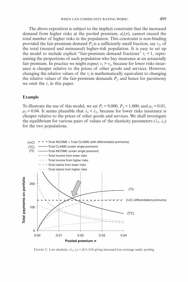
FIGURE 2: Low elasticity: (l1,l2) = (0.5, 0.9) giving increased loss coverage under pooling.

The above exposition is subject to the implicit constraint that the increaseddemand from higher risks at the pooled premium, d2(p), cannot exceed thetotal number of higher risks in the population. This constraint is non-bindingprovided the fair-premium demand P2 is a sufficiently small fraction, say t2, ofthe total (insured and uninsured) higher-risk population. It is easy to set upthe model to include explicit “fair-premium demand fractions” ti < 1, repre-senting the proportions of each population who buy insurance at an actuariallyfair premium. In practice we might expect t1 > t2, because for lower risks insur-ance is cheaper relative to the prices of other goods and services. However,changing the relative values of the ti is mathematically equivalent to changingthe relative values of the fair-premium demands Pi, and hence for parsimonywe omit the ti in this paper.

Example

To illustrate the use of this model, we set P1 = 9,000, P2 = 1,000; and m1 = 0.01,m2 = 0.04. It seems plausible that l1 < l2, because for lower risks insurance ischeaper relative to the prices of other goods and services. We shall investigatethe equilibrium for various pairs of values of the elasticity parameters (l1, l2)for the two populations.


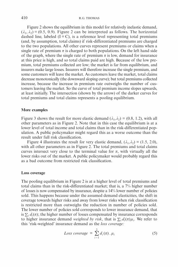
Figure 2 shows the equilibrium in this model for relatively inelastic demand,(l1, l2) = (0.5, 0.9). Figure 2 can be interpreted as follows. The horizontaldashed line, labeled (I = C), is a reference level representing total premiums(and, by assumption, total claims) if risk-differentiated premiums are chargedto the two populations. All other curves represent premiums or claims when asingle rate of premium p is charged to both populations. On the left hand sideof the graph, where the single rate of premium p is low, demand for insuranceat this price is high, and so total claims paid are high. Because of the low pre-mium, total premiums collected are low; the market is far from equilibrium, andinsurers make large losses. Insurers will therefore increase the single premium, andsome customers will leave the market. As customers leave the market, total claimsdecrease monotonically (the downward sloping curve); but total premiums collectedincrease, because the increase in premium rate outweighs the number of cus-tomers leaving the market. So the curve of total premium income slopes upwards,at least initially. The intersection (shown by the arrow) of the darker curves fortotal premiums and total claims represents a pooling equilibrium.

More examples

Figure 3 shows the result for more elastic demand (l1,l2) = (0.8, 1.2), with allother parameters as in Figure 2. Note that in this case the equilibrium is at alower level of total income and total claims than in the risk-differentiated pop-ulation. A public policymaker might regard this as a worse outcome than theresult under full risk classification.

Figure 4 illustrates the result for very elastic demand, (l1,l2) = (1.5, 2.0),with all other parameters as in Figure 2. The total premiums and total claimscurves intersect very close to the terminal value for p, with virtually all thelower risks out of the market. A public policymaker would probably regard thisas a bad outcome from restricted risk classification.

Loss coverage

The pooling equilibrium in Figure 2 is at a higher level of total premiums andtotal claims than in the risk-differentiated market; that is, a 7% higher numberof losses is now compensated by insurance, despite a 14% lower number of policiessold. This happens because under the assumed demand elasticities, the shift incoverage towards higher risks and away from lower risks when risk classificationis restricted more than outweighs the reduction in number of policies sold.The lower number of policies sold corresponds to lower insurance demand, thatis !i di(p); the higher number of losses compensated by insurance correspondsto higher insurance demand weighted by risk, that is !i di(p)mi. We refer tothis ‘risk-weighted’ insurance demand as the loss coverage:

Loss coverage = idi 1

2

=

! (p) . mi (5)

410 R.G. THOMAS

FIGURE 3: High elasticity: (l1,l2) = (0.8, 1.2) giving reduced loss coverage under pooling.

FIGURE 4: Very high elasticity: (l1,l2) = (1.5, 2.0), greatly reduced loss coverage under pooling.


0

100

200

0.00 0.01 0.02 0.03 0.04

Single premium π

Tota

l pay

men

ts o

n p

ort

folio

Total INCOME = Total CLAIMS (under differentiated premiums)

Total CLAIMS (under single premium)

Total INCOME (under single premium)

Total income from lower risks

Total income from higher risks

Total claims from lower risks

Total claims from higher risks

(I=C)

I = C (differentiated premiums)

(TC)(TI)

(TI)

(TC)

From a public policy perspective, loss coverage may be a better metric thannumber of policies sold for comparing the effects of alternative risk classifi-cation schemes. This is because loss coverage focuses on the expected lossescompensated by insurance (risk-weighted insurance demand), which seems abetter indicator of the social efficacy or benefit of insurance to the wholepopulation than number of policies sold (un-weighted insurance demand). Theloss coverage metric implies that the public policymaker places higher priorityon higher-risk individuals being insured: for example, insurance of one higher-risk individual is worth the same to the policymaker as insurance of two lower-risk individuals, if the probability of loss for each higher risk is twice that ofeach lower risk. In other words, insurances held by higher and lower-risk indi-viduals are regarded as equally desirable by the policymaker ex post, when alluncertainty about who will suffer a loss has been resolved; but insurances heldby higher-risk individuals are regarded as (risk-proportionately) more desirableby the policymaker ex ante.

For a public policymaker who uses the loss coverage metric, adverse selectionis not necessarily adverse. Sufficiently low demand elasticities are consistent witha moderate level of adverse selection, which may reduce insurance demand butincrease loss coverage (as shown in Figure 2). However, higher demand elas-ticities are consistent with “too much” adverse selection, which reduces bothinsurance demand and loss coverage (as shown in Figure 3, or in a more extrememanner in Figure 4). Under the loss coverage criterion, public policy on riskclassification can be seen as a question of degree: given the demand elasticitiesin a particular market, what restrictions on risk classification (if any) arerequired to induce the optimal degree of adverse selection, which maximisesthe loss coverage? Applications, extensions and limitations of the loss coverageconcept are discussed in greater detail in Thomas (2008).

When comparing alternative risk classification schemes, it is often conve-nient to define loss coverage in some normalized form. For example, later inthis paper we will use the ratio of expected losses covered under communityrating to expected losses covered under risk-differentiated premiums, sothat loss coverage is normalized to be 1 under risk-differentiated premiums.Alternatively, loss coverage could be normalized to be 1 under compulsoryinsurance of the whole population.

Generalizing for more than two risk groups

We can generalize the above to any distribution of risks in the population,rather than just higher and lower-risk groups, as follows. Let g be a risk para-meter, let mg be the expected loss for a risk with parameter g, let fg be the den-sity of the risks in the whole population, and let rg be the demand from riskswith risk parameter g. The expected demand for insurance from the wholepopulation is

E[rg] = gr# fg dg. (6)

412 R.G. THOMAS

FIGURE 5: Determination of pooled premium: a well-defined single equilibrium.

The loss coverage is

E[rg mg] = gr# mg fg dg. (7)

The expected claim per contract is

g

g

g

g

r

r

r f dg

r f dg

E

E

g

g g g=

m m

#

#8

8

B

B

(8)

and for an equilibrium in the presence of adverse selection, the pooled premiumneeds to be equal to this.

Graphically, an equilibrium premium is determined where the expected claimsper contract crosses the 45-degree line representing the premium, as shown atthe arrow in Figure 5. Note that if the actual premium increases above theequilibrium level, insurers make progressively increasing profits; if the pre-mium decreases, insurers make progressively increasing losses. The monotonicnature of the profit function implies that the equilibrium shown is stable andwell-defined.


3. POSSIBILITY OF MULTIPLE EQUILIBRIA

To generate multiple equilibria, the expected claims per contract must cross the45-degree single premium line more than once. Whether this is possible undersuitable elasticity conditions depends on the relative sizes of the higher andlower-risk populations, and their relative risks. Figure 6 shows the multiple

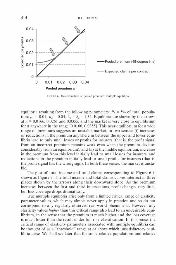
FIGURE 6: Determination of pooled premium: multiple equilibria.

equilibria resulting from the following parameters: P2 = 5% of total popula-tion; m1 = 0.01, m2 = 0.04; l1 = l2 = 1.35. Equilibria are shown by the arrowsat p = 0.0166, 0.0261 and 0.0355, and the market is very close to equilibriumfor p anywhere in the range [0.0166, 0.0355]. This near-equilibrium for a widerange of premiums suggests an unstable market, in two senses: (i) increasesor reductions in the premium anywhere in between the upper and lower equi-libria lead to only small losses or profits for insurers (that is, the profit signalfrom an incorrect premium remains weak even when the premium deviatesconsiderably from an equilibrium); and (ii) at the middle equilibrium, increasesin the premium from this level initially lead to small losses for insurers, andreductions in the premium initially lead to small profits for insurers (that is,the profit signal has the wrong sign). In both these senses, the market is unsta-ble.

The plot of total income and total claims corresponding to Figure 6 isshown as Figure 7. The total income and total claims curves intersect in threeplaces shown by the arrows along their downward slope. As the premiumincreases between the first and third intersections, profit changes very little,but loss coverage drops dramatically.

True multiple equilibria arise only from a limited critical range of elasticityparameter values, which may almost never apply in practice, and so do notcorrespond to any regularly observed real-world phenomena. However, anyelasticity values higher than this critical range also lead to an undesirable equi-librium, in the sense that the premium is much higher and the loss coverageis much lower than the result under full risk classification. In this sense, thecritical range of elasticity parameters associated with multiple equilibria canbe thought of as a “threshold” range at or above which unsatisfactory equi-libria arise. We shall see later that for some relative populations and relative

414 R.G. THOMAS

FIGURE 7: Multiple equilibria for l1 = l2 = 1.35.


risks, true multiple equilibria can never arise; but in such cases there may stillbe a critical range of elasticity values which lead to “near-equilibrium” overan extended range of values for the premium. Again, any elasticity valueshigher than this threshold range lead to an undesirable equilibrium, withmuch higher premium and much lower loss coverage than under full riskclassification.

Specifying the conditions for multiple equilibria

The conditions for multiple equilibria which were represented graphically inFigure 6 can be specified as follows. First note that when the premium is zero,average cost per claim exceeds the premium. When the premium is m2, averagecost per claim must be less than or equal to the premium. Hence if the aver-age cost per claim curve is to cross the premium line more than once, it mustat some point cross the premium line from below. This gives us two necessary

and sufficient conditions which must be satisfied simultaneously to give a“middle” equilibrium, which is one of at least three possible equilibria3:

>r

r

E

Ep 1

g

g g

22 mJ

L

KK

N

P

OO

8

8

B

B

(9)

and

r

r

E

Ep

g

g g=

m

8

8

B

B

(10)

In words, we can interpret these conditions as follows. As the premium pincreases, higher risks are attracted and lower risks drop out of the market; theaverage cost per claim increases, but generally at a lower rate than the (unit)increase in premium. For multiple equilibria to arise, the average cost per claimof the risks attracted by the pooled premium needs to increase faster than theunit increase in premium, over some interval of the feasible range for p; andsimultaneously, the average cost per claim needs to be equal to the premium p.Alternatively, we can think of the rate of increase of the average cost per claimas the price elasticity of the average risk attracted by the pooled premium.For multiple equilibria, this price elasticity needs to exceed 1, over some inter-val of the feasible range for p; and simultaneously, the average cost per claimneeds to be equal to the premium p.

We can investigate this further using the two-populations model specifiedearlier. l1 and l2 were previously both regarded as free parameters, but a flexiblealternative (with obvious extensions for more than two risk groups) is to spec-ify a “base” elasticity, say l, for the larger, lower-risk population 1 and then set

l mm

la

21

2= d n (11)

where a is an index for the variation of the fair-premium demand elasticity asthe fair premium itself changes. This specification is convenient for expositorypurposes because it allows us to plot equilibrium premiums and loss coveragesagainst the single elasticity parameter l. There are no absolute theoretical lim-its on the value of a, but it can be seen that 0 ≤ a ≤ 1 may be a reasonablerange –

– if a = 0, fair-premium demand elasticity is the same for both risk groups;– if a < 0, fair-premium demand elasticity is inversely related to the fair pre-

mium; this seems unlikely, because it implies a negative income effect fromthe higher-risk fair premium representing a larger part of the consumer’s totalbudget constraint;

416 R.G. THOMAS

3 With the form of insurance demand used in this paper, it does not appear to be possible to gener-ate an average cost per claim curve which crosses the premium line more than three times; but moreidiosyncratic demand specifications may be capable of doing so.

– if a > 1, fair-premium demand elasticity increases more than proportion-ately with the fair premium; this is possible, if the fair premium for higherrisks represents a large part of their total budget constraint; but for the typ-ical case where insurance is a small part of the consumer’s total budget con-straint, it seems unlikely.

We will show figures in tables for a = 0, 1/3 and 2/3. It turns out that the qual-itative pattern of results is similar for all these values, and so for brevity allgraphs are based on a = 1/3 only. This seems a reasonable value, in that itallows for fair-premium demand elasticity in the higher-risk population to bemoderately higher than in the lower-risk population, as is expected from theincome effect (ie the higher-risk fair premium represents a larger part of theconsumer’s total budget constraint). There is no specific empirical evidence ortheoretical argument to support a = 1/3, but the qualitatively similar patternof results obtained from other values in the range 0 ≤ a ≤ 1 suggests that thisis not critical to our results.

We set P1 : P2 = 95:5, rather than 90:10 as in section 2 above4, and hereafterdenote this by the phrase “5% higher-risk population fraction”. Recall thatfor multiple equilibria, the average cost per claim needs to cross the 45-degreepremium line from below; that is, the average cost per claim for the risksattracted by the pooled premium needs to increase faster than the unit increase inthe premium, over some part of the feasible range for the premium. Intuitively,this could occur either because the risk difference between the two popula-tions is high, or because fair-premium demand elasticity is high; and the higherthe risk difference, the smaller the fair-premium demand elasticity required toproduce multiple equilibria. This intuition is confirmed in Table 1, which showsthe critical ranges of fair-premium demand elasticities l which generate mul-tiple equilibria, for various relative risks.

What happens if the fair-premium demand elasticity is near, but not within,the critical range which generates multiple equilibria? If the elasticity is slightlyhigher, the equilibrium premium will be slightly higher than the highest of themultiple equilibria; and if the elasticity is slightly lower, the equilibrium pre-mium will be slightly lower than the lowest of the multiple equilibria. In effect,the multiple equilibria correspond to a “jump” in the plot of equilibrium pre-mium or loss coverage against the fair-premium demand elasticity l. This“jump” effect is illustrated in Figure 8, which shows equilibrium premium andcorresponding loss coverage as a function of fair-premium demand elasticity lfor the case m2 /m1 = 4 and a = 1/3 (i.e. the central cell of Table 1). The dashedhorizontal line in the left panel in Figure 8 represents the population-weightedaverage of the risk-differentiated premiums. The dashed horizontal line in theright panel represents the loss coverage if risk-differentiated premiums are


4 The reason for starting our investigations with a population ratio of 95:5 rather than 90:10 asbefore is that we shall see later that given the reasonable constraint l2 ≥ l1, a 90:10 population rationever produces multiple equilibria (Table 4 later in the paper gives details).

charged; this is normalized to a value of 1. The gaps left in the premium andloss coverage curves for 1.33 < l < 1.40 correspond to the region where anyvalue of l generates three equilibria, which are located between the upper andlower limits indicated by the ends of the curves on either side of the gaps.The three crosses show the multiple solutions generated for the specimen valuel = 1.35; an analogous triad of solutions arises for any l in the range 1.33 <l < 1.40.

The characteristic sigmoid pattern of the graphs shown in Figure 8, witha jump in the premium and loss coverage around the region of multiple solutions,provides a basis for distinguishing between an archetypal adverse selectionspiral, with a large increase in premium and reduction in loss coverage com-pared to the result under risk-differentiated premiums, and other scenarioswhere the insurance system stabilizes after only a modest rise in premiums.If fair-premium demand elasticity is at or above the threshold range whichgenerates multiple solutions, we have an archetypal adverse selection spiral.But if fair-premium demand elasticity is below the threshold range, the equi-librium premium is only slightly above the population-weighted average of therisk-differentiated premiums.

From a public policy viewpoint, any equilibrium for l > 1.33 in Figure 8might be regarded as a bad outcome from restricted risk classification, becauseloss coverage is drastically reduced as compared with the result if risk-differ-entiated premiums are charged. For lower values of l, say l < 1, the reductionin loss coverage is much smaller; a public policymaker might in some casesregard this as a “price worth paying” to satisfy other policy objectives such associal solidarity. For l < 0.71, loss coverage actually increases slightly underrestricted risk classification as compared with risk-differentiated premiums.In such cases, the adverse selection resulting from restricted risk classification

418 R.G. THOMAS

TABLE 1

FAIR-PREMIUM DEMAND ELASTICITIES l WHICH GENERATE MULTIPLE EQUILIBRIA, FOR VARIOUS

RELATIVE RISKS (5% HIGHER-RISK POPULATION FRACTION)

Relative risk Ranges for fair-premium demand elasticity lm2 / m1 which generate multiple equilibria

(eg “2.76 – 3.26” denotes 2.76 < l < 3.26)

a = 0 a = 1/3 a = 2/3

2 2.76 – 3.26 2.74 – 3.15 2.72 – 3.05 3 1.70 – 1.87 1.68 – 1.78 1.65 – 1.704 1.33 – 1.40 1.30 – 1.32 ≈ 1.27†5 1.13 – 1.16 ≈ 1.15† ≈ 1.06†6 1.002 – 1.012 ≈ 1.0† ≈ 0.95†

† There are no true multiple equilibria for these combinations of a and relative risks. The values shownare those corresponding to “near multiple equilibria”.

FIGURE 8: Equilibrium premium and loss coverage as a function of l for 5% higher-risk populationfraction; crosses show specimen multiple solutions for l = 1.35.

is arguably not “adverse” at all; a public policymaker might regard the increasedloss coverage as a good outcome.5

What if the higher-risk fraction of the population differs from the 5%assumed in Table 1? If the higher-risk fraction is smaller, for example a higher-risk fraction of 2†% of the total population, the demand elasticity parameterswhich generate multiple equilibria increase, as shown in Table 2. In onesense, this makes multiple equilibria less plausible: some of the required demand


5 The increase in loss coverage for l < 0.71 is very small in Figure 8, but larger increases can be gen-erated if the higher-risk population is a larger fraction of the total population, or if the difference infair-premium demand elasticities between the two populations is larger; for example, see Figure 10 inthis paper.

TABLE 2

FAIR-PREMIUM DEMAND ELASTICITIES l WHICH GENERATE MULTIPLE EQUILIBRIA, FOR VARIOUS

RELATIVE RISKS (2†% HIGHER-RISK POPULATION FRACTION)

Relative risk Ranges for fair-premium demand elasticity lm2 / m1 which generate multiple equilibria

(eg “2.98 – 4.94” denotes 2.98 < l < 4.94)

a = 0 a = 1/3 a = 2/3

2 2.98 – 4.94 2.95 – 4.83 2.93 – 4.763 1.83 – 2.71 1.82 – 2.60 1.81 – 2.544 1.44 – 1.96 1.42 – 1.85 1.40 – 1.795 1.23 – 1.58 1.21 – 1.47 1.19 – 1.426 1.09 – 1.35 1.08 – 1.25 1.05 – 1.20

FIGURE 9: Equilibrium premium and loss coverage as a function of l for 2†% higher-risk populationfraction; crosses show specimen multiple solutions for l = 1.70.

elasticity parameters are now very high. But in a different sense, the smallerhigher-risk fraction makes it easier to generate multiple equilibria: as shown inTable 2, multiple equilibria are generated by l in wider ranges than in Table 1.

Figure 9 shows equilibrium premium and corresponding loss coverage asa function of fair-premium demand elasticity for the case m2 /m1 = 4 and a = 1/3(ie the central cell of Table 2). The heavy dashed horizontal lines represent thepopulation-weighted average of the risk-differentiated premiums (in the leftpanel), and the loss coverage if risk-differentiated premiums are charged (in theright panel). The gaps left in the plots for 1.42 < l < 1.85 correspond to theregion where any value of l generates three equilibria, which are locatedbetween the between the upper and lower limits indicated by the ends of thecurves on either side of the gap. The three crosses show the multiple solutionsgenerated by l = 1.70; an analogous triad of solutions arises for any l in therange 1.42 < l < 1.85. It can be seen that for any l ≤ 1.42, the equilibriumpooled premium is only very slightly higher than the population-weightedaverage of the risk-differentiated premiums (the horizontal dashed line at p =0.01075). Loss coverage is generally slightly lower than under risk-differenti-ated premiums, unless l < 0.73, where it becomes very slightly higher. For anyl ≥ 1.85, the equilibrium pooled premium is far above the population-weightedaverage premium, and loss coverage is drastically reduced.

What happens if the higher-risk fraction of the population is more than 5%?If the higher-risk fraction is say 10%, then to generate multiple equilibria, l2

substantially less than l1 is required, as shown in Table 3. However l2 sub-stantially less than l1 is often rather implausible. The higher price of insurancefor higher risks, relative to the price of other goods and services, lead us toexpect that l2 would generally be higher than l1. Given the reasonable con-straint l2 ≥ l1, we can specify a critical fraction for the higher-risk population

420 R.G. THOMAS

which ensures that no multiple equilibria arise. This critical fraction is shownfor various population relative risks in Table 4.

When the higher-risk population fraction only modestly exceeds the frac-tion required to ensure no multiple equilibria, there is still a region of “nearmultiple equilibria”, where the equilibrium premium and the corresponding losscoverage change rapidly with changes in l. This effect is illustrated in the upperpanels of Figure 10, which show the plots for a 10% higher-risk populationfraction, with m2 /m1 = 4 and a = 1/3. The region of “near multiple equilibria”is centred around l ≈ 1.23; it can be seen that the equilibrium premium and losscoverage plots against l display sigmoid and reverse sigmoid patterns respectively,with their highest rates of change centred around l ≈ 1.23. As the higher-risk pop-ulation fraction is increased further, the sigmoid and reverse sigmoid patternsgradually flatten out. This effect is illustrated in the lower panels in Figure 10,which show the plots for a 20% higher-risk population fraction, still with m2 /m1

= 4 and a = 1/3. The less skewed population (80:20 instead of 90:10) leads toa less steep “jump” between the low-premium and high-premium regions.


TABLE 3

APPROXIMATE FAIR-PREMIUM DEMAND ELASTICITIES l1 AND l2 REQUIRED TO PRODUCE MULTIPLE EQUILIBRIA,FOR VARIOUS RELATIVE RISKS (10% HIGHER-RISK POPULATION FRACTION)

Relative risk Approximate fair-premium demand elasticity li

m2 / m1 required to produce multiple equilibria

l1 l2

2 ≈2.60 <1.443 ≈1.60 <0.524 ≈1.23 <0.285 ≈1.05 <0.11

≥ 6 Cannot generate multiple equilibria

TABLE 4

THRESHOLD HIGHER RISK POPULATION (AS FRACTION OF TOTAL POPULATION) REQUIRED TO ENSURE NO

MULTIPLE EQUILIBRIA, GIVEN l2 ≥ l1

Relative risk Threshold higher risk population P2

m2 / m1 (as fraction of total population) required toensure no multiple equilibria, given l2 ≥ l1

2 > 9.0%3 > 7.3%4 > 6.2%5 > 5.6%6 > 5.1%

FIGURE 10: Equilibrium premium and loss coverage as a function of fair-premium demand elasticity,m2 /m1 = 4.

To summarize the numerical results in Tables 1 to 4 and Figure 10, we makethe following observations.

– Variations in the parameter a have only a small effect on the demand elas-ticity parameter required to generate multiple equilibria. This can be under-stood as follows. The parameter a indexes the demand elasticity “premium”or “margin” for the higher-risk population over that of the lower-risk popu-lation. The much larger size of the lower-risk population means that at mostequilibria, most of the income and claims relate to the lower-risk population.Hence the results are driven mainly by the “base” demand elasticity parameter,with only a small effect from the demand elasticity “premium” or “margin”for the higher-risk population.

422 R.G. THOMAS

– As relative risk (m2 /m1) increases, the demand elasticity parameter requiredto generate multiple equilibria decreases. This can be understood as follows.Recall that multiple equilibria require the average cost per claim for risksattracted by the pooled premium to be increasing faster over some range thanthe unit increase in the premium. This can happen either because the demandresponse to the premium increase is high, or because the difference in therisks is high.

– As relative risk (m2 /m1) increases, the range of demand elasticity parameterswhich generate multiple equilibria becomes narrower. This can be understoodby reference to Figure 6, as follows. As the demand elasticity parameterincreases through the critical range, the scenario of three intersectionsbetween average claim costs and premium shown in Figure 6 moves towardsa single intersection at a premium above the highest of the three inter-sections. For the multiple equilibria to disappear, the average cost per claimcurve in Figure 6 must move upwards sufficiently so as to eliminate its inter-sections with the 45-degree premium line at lower premiums. If the relativerisk ( m2 /m1) is low, the average cost per claim changes only slowly as theelasticity parameter (and hence insurance demand) changes; and hence themultiple intersections in Figure 6 persist for a wider range of demand elas-ticity parameters.

– As the higher-risk fraction of the population increases, the demand elastic-ity parameter required to generate multiple equilibria decreases. However,if the higher-risk fraction of the population exceeds a threshold, multipleequilibria cannot arise, given the reasonable constraint l2 ≥ l1. This can beunderstood as follows. With a larger higher-risk fraction, the higher-riskpopulation makes a material contribution to the average cost per claim overthe full range ( m1, m2] of feasible premium levels. As p is increased, lower riskshave a higher propensity to leave the market than higher risks; but the mate-rial weighting of the higher risks, at all premium levels, means that the higherrate of exit of lower risks never raises the rate of change of the average costper claim above 1, with the average cost per claim also simultaneously equalto the premium. In effect, the material weighting of higher risks in the aver-age cost per claim over the full range ( m1, m2] of feasible premium levels actsas a “drag” on the rate of change of the average cost per claim. This “drag”on the rate of change of the average cost per claim from the weighting ofhigher risks also increases with the relative risk ( m2 /m1). The latter pointexplains the last line in Table 3: for high relative risk, m2 /m1 ≥ 6, even verylow l2, much less than l1, cannot generate multiple equilibria6.


6 For further insight into this “drag” from a larger higher-risk population fraction, consider a casewhere the skew is reversed, so that the higher-risk population forms the larger part of the total pop-ulation, say P2 = 90%. In this case, it is obvious that over the full range ( m1, m2] of feasible premiumlevels, the lower risks will always contribute very little to the average cost per claim. The averagecost per claim will always be close to the risk level for the higher-risk population, and will changeonly slightly as p changes.

Conditions which preclude multiple equilibria irrespective of relative populationsand risks

It is also possible to specify broad regions of the parameter space for (l1, l2)where multiple equilibria can never arise, irrespective of the higher-risk popu-lation fraction and the relative risk. First note that the total claims curve inFigures 2, 3, 4 and 7 must always slope downwards over the full feasible range( m1, m2 ]. Multiple equilibria arise if the total income curve intersects the totalclaims curve more than once in the range ( m1, m2]. This cannot happen if thetotal income curve slopes upwards over the full range ( m1, m2]. The total incomecurve is the sum of the income from populations 1 and 2. So if the total incomecurve for each population slopes upwards over the full range – that is, there isno maximum in the premium income curve below m2 – then multiple equilibriacannot occur.

The condition for a maximum in total premium income from population i,say Fi, is

i l./

dp

p pl p m0 1i i

i&2

2= =

]^^

ghh (12)

For population 1, note that p /m1 ≤ m2 /m1 and hence

l1( m2 /m1)l1 ≤ 1 (13)

is a sufficient condition for the absence of a maximum in the premium incomecurve F1 below m2. But m2 /m1 > 1, and hence the condition (13) for absence ofa maximum in F1 below m2 requires l1 ≤ 1. For any given relative risk ( m2 /m1),the maximum value of l1 which admits a maximum in F1 below m2 can thenbe found as the unique solution for l1 of

mm

l / l

2

111= 1d n (14)

Moving on to population 2, and applying equation (12) above, note thatp /m2 ≤ 1. Hence l2 < 1 is a sufficient condition for the absence of a maximumin F2 below m2.

The above conditions lead to Table 5, which shows for a range of relativerisks ( m2 /m1) the regions of the (l1, l2) parameter space in which multiple equi-libria can never occur, irrespective of the relative sizes and fair-premium take-ups of the two populations.

The conditions in Table 5 are sufficient to ensure that multiple equilibriacannot occur, irrespective of the higher-risk population fraction; but they arenot necessary conditions. They can be thought of as conditions to give a graphof total premiums and total claims of the type characterized by Figure 2: thetotal income curve slopes upwards over the entire range ( m1, m2 ]. But even ifthe total income curve slopes downwards towards the upper end of the range

424 R.G. THOMAS

( m1, m2 ], it may intersect the total claims curve only once: that is, a graph ofthe type characterized by Figure 3 or Figure 4. Therefore the li can be higherthan the values in Table 5 and still be “safe” in the sense of not produce mul-tiple equilibria. Multiple equilibria arise only when the graph is of the typecharacterized by Figure 7.

Comparison with empirical demand elasticities

The fair-premium demand elasticity parameters in Tables 1 to 5 can be comparedwith empirical estimates of demand elasticity for various classes of insurance.We defined demand elasticity using absolute values for convenience in thispaper, but the estimates in empirical papers are generally given with the neg-ative sign, and so we quote them in that form. For example, for yearly renewableterm insurance in the US, an estimate of –0.4 to –0.5 has been reported (Paulyet al, 2003). A questionnaire survey about life insurance purchasing decisionsproduced an estimate of –0.66 (Viswanathan et al, 2007). For private healthinsurance in the US, several studies estimate demand elasticities in the rangeof 0 to –0.2 (Chernew et al., 1997; Blumberg et al., 2001; Buchmueller and Ohri,2006). For private health insurance in Australia, Butler (1999) estimates demandelasticities in the range –0.36 to –0.50 (higher than in the US, perhaps becauseAustralia’s universal Medicare is a better substitute for private insurance thanis available to most people in the US). These magnitudes are significantly lowerthan the threshold values of fair-premium demand elasticity required to gen-erate multiple equilibria (or above the threshold, low-coverage equilibria) inour model. Demand elasticity for some types of insurance might be higher,particularly where there is a good substitute for the insurance. However,actual demand elasticitity magnitudes significantly lower than the thresholdvalues which lead to multiple equilibria (or above the threshold, low-coverageequilibria) in our model may explain why some insurance markets appear to


TABLE 5

REGIONS OF PARAMETER SPACE FOR (l1, l2) WHERE MULTIPLE EQUILIBRIA CANNOT OCCUR,IRRESPECTIVE OF POPULATION FRACTIONS (P1, P2)

Relative risk Absence of multiple equilibria is assuredm2 / m1 for the following parameter pairs:

l1 l2

2 <0.641 <13 <0.548 <14 <0.500 <15 <0.469 <16 <0.448 <1

operate reasonably well under community rating, without the collapse in cov-erage which insurance folklore suggests.

The remarks in the preceding paragraph are made in the context that allinsurers are required to operate the same risk classification regime, as wasassumed when setting up the model in section 2 of the paper. The remarkswill probably not apply where different insurers are permitted to compete byoffering different risk classification regimes. In this scenario, where differentinsurers’ products are close substitutes offered on different underwriting terms,it seems plausible that the demand elasticity for insurance from a particularinsurer might be much higher than demand elasticity for insurance from anyinsurer. The “adverse selection spiral” may then be a good description of thefate of one insurer which does not classify risks adequately in a setting whereothers insurers do7. But this does not necessarily mean that it is a good descrip-tion of the fate of a market where no insurers classify risk.

4. CONCLUSION

This paper has used a simple model with two populations, one higher-risk andone lower-risk, to investigate insurance market outcomes when insurers arenot permitted to differentiate premiums by risk level. Market outcomes werecharacterized by the equilibrium pooled premium when risk classificationwas restricted, and the corresponding risk-weighted insurance demand or “losscoverage.” It was suggested that from a public policy perspective, loss coverage(risk-weighted insurance demand) might be a better metric from a public policyperspective than number of policies sold (un-weighted insurance demand),because loss coverage focuses on the expected losses actually compensated byinsurance.

For the model in this paper, the main results are as follows. Insurance mar-ket outcome in the absence of risk classification can be related to a parameterfor the elasticity of demand for insurance at an actuarially fair premium, thatis the “fair-premium demand elasticity.” High fair-premium demand elasticityleads to an equilibrium premium close to the risk of the higher-risk popula-tion, and a much lower loss coverage than under risk-differentiated premiums.This can be thought of as the conclusion of an archetypal adverse selectionspiral. From a public policy perspective, it might be considered a bad outcomefrom community rating. But for sufficiently low fair-premium demand elas-ticity, this collapse in coverage does not occur; instead, the market stabilizeswith a premium only slightly higher than the population-weighted average ofrisk-differentiated premiums, and relatively high loss coverage – possibly higherthan under more complete risk classification. From a public policy perspective,this might be considered a good outcome from community rating.

426 R.G. THOMAS

7 Footnote 2 summarises an example, as reported in Cutler & Reber (1998).

The ranges for the demand elasticity parameter characterized above as“high” and “low” are separated by a threshold range for the parameter whichleads to an unstable market outcome – either multiple equilibria (that is, morethan one pooled premium is capable of equilibrating insurers’ revenue andclaims), or near-equilibria for an extended range of premium values. Generally,the threshold range for the fair-premium demand elasticity parameter at orabove which an unsatisfactory outcome arises in the model in this paper appearshigher than the demand elasticity values which have been estimated in empir-ical studies of a number of insurance markets. The high demand elasticitywhich is required to generate an unsatisfactory outcome offers a possible expla-nation of why some insurance markets appear to operate reasonably well undercommunity rating, without the collapse in coverage which insurance folkloresuggests. Finally, it is emphasized that these conclusions are based on a specificmodel, which may require some generalization before the results are widelyapplied.

REFERENCES

BLUMBERG, L., NICHOLS, L. and BANTHIN, J. (2001) ‘Worker decisions to purchase health insur-ance’. International Journal of Health Care Finance and Economics, 1: 305-325.

BUCHMUELLER, T. and DINARDO, J. (2002) ‘Did community rating induce an adverse selectiondeath spiral? Evidence from New York, Pennsylvania and Connecticut’. American EconomicReview, 92: 280-294.

BUCHMUELLER, T.C. and OHRI, S. (2006) ‘Health insurance take-up by the near-elderly’. HealthServices Research, 41: 2054-2073.

BUTLER, J.R. (2002) ‘Policy change and private health insurance: Did the cheapest policy do thetrick?’. Australian Health Review, 25(6): 33-41.

CHERNEW, M., FRICK, K. and MCLAUGHLIN, C. (1997) ‘The demand for health insurance coverageby low-income workers: Can reduced premiums achieve full coverage?’. Health ServicesResearch, 32: 453-470.

CUTLER, D. and REBER, S. (1998) ‘Paying for health insurance: the trade-off between competi-tion and adverse selection’. Quarterly Journal of Economics, 113: 433-466.

DE JONG, P. and FERRIS, S. (2006) ‘Adverse selection spirals’, ASTIN Bulletin, 36: 589-628.GALE, A.P. (2007) One price fits all. Paper presented to the Institute of Actuaries Australian

Biennial Convention, 2007.Institute of Actuaries Australia (1994) Insurance & superannuation risk classification policy. IAA,

Sydney. 16 pages.MACDONALD, A.S. (1997) ‘How will improved forecasts of individual lifetimes affect underwrit-

ing?’ Philosophical Transactions of the Royal Society B, 352: 1067-1075, and (with discussion)British Actuarial Journal, 3; 1009-1025 and 1044-1058.

MACDONALD, A.S. (1999) ‘Modeling the impact of genetics on insurance’. North American Actu-arial Journal, 3(1): 83-101.

MACDONALD, A.S. (2003) ‘Moratoria on the Use of Genetic Tests and Family History for Mort-gage-Related Life Insurance’. British Actuarial Journal 9: 217-237.

MACDONALD, A.S. and TAPADAR, P. (2007) ‘Multifactorial disorders and adverse selection: epi-demiology meets economics’. Forthcoming in Journal of Risk and Insurance, 2010.

PAULY, M.V., WITHERS, K.H., VISWANATHAN, K.S., LEMAIRE, J., HERSHEY, J.C., ARMSTRONG, K.and ASCH, D.A. (2003) ‘Price elasticity of demand for term life insurance and adverse selec-tion’, NBER Working Paper, 9925.

ROSE, C. (1993) ‘Equilibrium and adverse selection’. RAND Journal of Economics, 24: 559-569.


SIEGELMAN, P. (2004) ‘Adverse selection in insurance markets: an exaggerated threat’, Yale LawJournal 113: 1225-1271.

VISWANATHAN, K.S., LEMAIRE, J., WITHERS, K., ARMSTRONG, K., BAUMRITTER, A., HERSHEY, J.,PAULY, M. and ASCH, D.A. (2006) ‘Adverse selection in term life insurance purchasing dueto the BRCA 1/2 Genetic Test and elastic demand’. Journal of Risk and Insurance, 74: 65-86.

THOMAS, R.G. (2008) ‘Loss coverage as a public policy objective for risk classification schemes’.Journal of Risk & Insurance 75: 997-1018.

WILSON, C.A. (1979) ‘Equilibrium and adverse selection’. American Economic Review, 69: 313-317.

WILSON, C.A. (1980) ‘The nature of equilibrium in markets with adverse selection’. Bell Journalof Economics, 11: 108-130.

R. GUY THOMAS

School of Mathematics, Statistics & Actuarial ScienceUniversity of KentCanterbury CT2 7NFUnited KingdomE-mail: [email protected]

428 R.G. THOMAS

demand elasticity, risk classification and loss … · ticity in an insurance market where risk...

Documents