Demand Systems for Empirical Work in IO∗

John Asker, Allan Collard-Wexler

October 5, 2007

Overview

Demand systems often form the bedrock upon which empirical work in in-dustrial organization rest. The next 2.5 lectures aim to introduce you to thedifferent ways empirical researchers have approached the issue of demand es-timation in the applied contexts that we typical confront as IO economists.

I start by talking about the different instances in which demand estima-tion arises and the core problems we face when estimating demand. Afterreviewing standard data forms, I will then go on to talk about the standardapproaches to demand estimation and their advantages and disadvantages.All these approaches try to deal with the problem of estimating demand whenwe are in a market with many, differentiated goods. Specific papers will beused to illustrate the techniques once they have been discussed.

I will expect you to remember your basic econometrics, particularly thestandard endogeniety problem of estimating demand (see Working 1927 orthe treatment in standard econometrics texts e.g. Hayashi 2000 in Ch 3).

There has been an explosion in the sophistication of technique used indemand estimation the last decade, due to a combination of advances ineconometric technique, computation and data availability.

∗These notes draw from a variety of sources, in particular Ariel Pakes’ lecture notesfrom when I was a grad student. I have rewritten large amounts so any mistakes are mine.

1

Why spend time on Demand Systems?

• In IO we usually care about care about comparative statics of one formor another. Usually demand is important to this: Think about pre andpost merger pricing, tax incidence, monopoly vs duopoly pricing, effectof predative pricing policies etc.

• Also care about welfare impacts: need a well specified demand systemfor welfare calculations

• In IO and Marketing there is considerable work on advertising whichusually involves some demand estimation. This about policy questionsof direct-to-consumer drug adverts or advertising as a barrier to entry.

• Understanding the cross-price elasticities of good is often crucial to“preliminary” issues in policy work, such as market definition in an-titrust cases. We will talk about the antitrust applications of demandmodels in the third lecture. Note that this is the largest consumer ofPh.D’s in Empirical I.O. by a long shot!

• Determinants of Market Power: should we allow two firms to merge?Is there collusion going on in this industry (unusually large markups)?

• Determinants of Innovation: once you have markups you know whichproducts a firm will want to produce (SUV’s, cancer drugs instead ofmalaria treatments).

• Value of Innovation: compute consumer surplus from the introductionof a new good (minivans and CAT scan).

• The tools used in demand estimation are starting to be applied in avariety of other contexts to confront empirical issues, of there is likelyto be some intellectual arbitrage for your future research.

Data...

The data that we should have in mind when discussing demand estimationtends to look as follows:

2

• The unit of observation will be quantity of product purchased (say 12oz Bud Light beer) together with a price for a given time period (saya week) at a location (Store, ZIP, MSA...).

• There is now a large amount of consumer-level purchase data collectedby marketing firms (for instance the ERIM panel used by AckerbergRAND 1997 to look at the effects of TV ads on yogurt purchases).However, the vast majority of demand data is aggregated at some level.

• Note that you have a lot of information here: You can get many char-acteristics of the good (Alcohol by volume, calories, etc) from the man-ufacturer or industry publications or packaging since you know thebrand. The location means we can merge the demand observation withcensus data to get information on consumer characteristics. The datemeans we can look at see what the spot prices of likely inputs were atthe time (say gas, electricity etc).

• So can fill in a lot of blanks

• Typical data sources: industry organizations, marketing and surveyfirms (e.g. AC Nielson), proprietary data from manufacturer, market-ing departments have some scanner data online (e.g. Chicago GSB).

• The survey of consumer expenditures also has some information onperson-level consumption on product groups like cars or soft-drinks.

Example: Autos

Bresnahan 1987: Competition and Collusion in 1950s Auto MarketWanted to examine the hypothesis that the dramatic decrease in the

price of Autos in 1955 was due to the temporary breakdown of a collusiveagreement. His idea was to assume that marginal costs were not varying andthen ask whether the relationship between pricing and demand elasticitieschanged in a manner consistent with a shift from collusion to oligopolisticpricing.

He exploits data on P and Q for different makes of Auto. He has about85 models over 3 years.

The “magic” in these approaches is using demand data to back outmarginal costs, without any cost data.

3

Question: What are the empirical modelling issues here?

Approaches to demand estimation

Approaches breakdown along the following lines:

• single vs multi-products

• representative agent vs heterogenous agent

• within multi-product: whether you use a product space or characteristicspace approach

Revision: Single Product Demand Estimation

• Start with one homogenous product.

• Assume an isolelastic demand curve for product j in market t:

ln(qjt) = αjpjt +Xjtβ + ξjt (1)

Note that price elasticity ηjjt = αjpjt.

• Xjt could just be an intercept for now (constant term).

• ξjt are unobserved components of demand (often called unobservedproduct quality).

Let’s go to the supply side for a second since the firm selling product j ispresumably allowed to choose it’s price (if we are in an unregulated market).

Firms get to choose prices. The pricing rule of a monopolist is to maximizeprofits:

πjt = (pjt − cjt)qjt (2)

(assuming constant marginal costs for now)

4

The F.O.C. for this problem is:

∂πjt

∂pjt

= qjt + (pjt − cjt)∂qjt∂pjt

pjt = cjt − qjt∂pjt

∂qjt

pjt = cjt − pjt1

ηjj

pjt =cjt

1 + 1ηjj

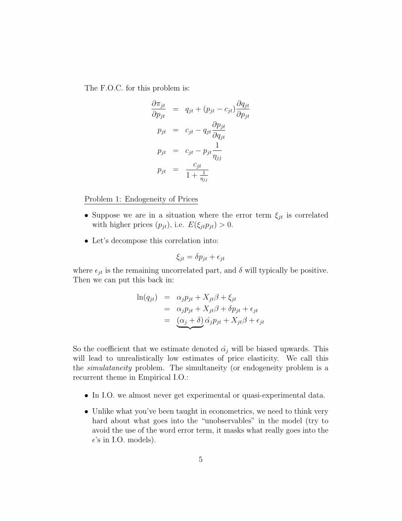
Problem 1: Endogeneity of Prices

• Suppose we are in a situation where the error term ξjt is correlatedwith higher prices (pjt), i.e. E(ξjtpjt) > 0.

• Let’s decompose this correlation into:

ξjt = δpjt + εjt

where εjt is the remaining uncorrelated part, and δ will typically be positive.Then we can put this back in:

ln(qjt) = αjpjt +Xjtβ + ξjt

= αjpjt +Xjtβ + δpjt + εjt

= (αj + δ)︸ ︷︷ ︸ αjpjt +Xjtβ + εjt

So the coefficient that we estimate denoted αj will be biased upwards. Thiswill lead to unrealistically low estimates of price elasticity. We call thisthe simulataneity problem. The simultaneity (or endogeneity problem is arecurrent theme in Empirical I.O.:

• In I.O. we almost never get experimental or quasi-experimental data.

• Unlike what you’ve been taught in econometrics, we need to think veryhard about what goes into the “unobservables” in the model (try toavoid the use of the word error term, it masks what really goes into theε’s in I.O. models).

5

• Finally, it is a very strong assumption to think that the firm does notreact to the unobservable because it does not see it (if I don’t have thedata, why should a firm have this data)!

• Remember that these guys spend their lives thinking about pricing.

• Moreover, won’t firms react if they see higher than expected demandyesterday?

• Note: From here on, when you are reading the papers, think hard about“is there an endogeneity problem that could be generating erroneousconclusions, and how do the authors deal with this problem”.

Review: What is an instrument

The broadest definition of an instrument is as follows, a variable Z such thatfor all possible values of Z:

Pr[Z|ξ] = Pr[Z|ξ′]

But for certain values of X we have

Pr[X|Z] = Pr[X|Z ′]

So the intuition is the Z is not affected by ξ, but has some effect on X.The usual way to express these conditions is that an instrument is such that:E[Zξ] = 0 and E[XZ] 6= 0.

This is a representative agent model to make it a heterogenous agentmodel we would have to build a micro model to make sure everything aggre-gated nicely, and then end up estimating something that looked somethinglike

qj =

∫γig (dγ) +

∫αipjf (dα) + βxj + εj (3)

Where αi ∼ F (α|θ) and γi ∼ G (α|τ) with θ and τ to be estimated. Thisis called a random coefficient model. Identification of the random coefficientparameters comes from differences in the sensitivity of demand to movementsin price, as the price level changes. (Think about whether the model wouldbe identified if the demand intercept were constant across all consumers)

6

Multi-product Systems

Now let’s think of a multiproduct demand system to capture the fact thatmost products have substitutes for each other.

ln q1 =∑j∈J

γ1jp1t + βx1t + ξ1t

...

ln qJ =∑j∈J

γJjpJt + βxJt + ξJt

Product vs Characteristic Space

We can think of products as being:

• a single fully integrated entity (a lexus SUV); or

• a collection of various characteristics (a 1500 hp engine, four wheelsand the colour blue).

It follows that we can model consumers as having preferences overproducts, or over characteristics.

The first approach embodies the product space conception of goods, whilethe second embodies the characteristic space approach.

Product Space: disadvantages for estimation

[Note that disadvantages of one approach tend to correspond to the advan-tages of the other]

• Dimensionality: if there are J products then we have in the order of J2

parameters to estimate to get the cross-price effects alone.

– Can get around this to some extent by imposing more structure inthe form of functional form assumptions on utility: this leads to”grouping” or ”nesting” approaches whereby we group productstogether and consider substitution across and within groups asseparate things - means that ex ante assumptions need to bemade that do not always make sense.

7

• hard to handle the introduction of new goods prior to their introduction(consider how this may hinder the counterfactual exercise of workingout welfare if a product had been introduced earlier - see Hausman onCell Phones in Brookings Papers 1997 - or working out the profits toentry in successive stages of an entry game...)

Characteristic Space: disadvantages for estimation

• getting data on the relevant characteristics may be very hard and deal-ing with situations where many characteristics are relevant

• this leads to the need for unobserved characteristics and various com-putational issues in dealing with them

• dealing with new goods when new goods have new dimensions is hard(consider the introduction of the laptop into the personal computingmarket)

• dealing with multiple choices and complements is a area of ongoingresearch, currently a limitation although work advances slowly eachyear.

We will explore product space approaches and then spend a fair amountof time on the characteristic space approach to demand. Most recent workin methodology has tended to use a characteristics approach and this alsotends to be the more involved of the two approaches.

8

Product Space Approaches: AIDS Models

I will spend more than an average amount of time on AIDS (Almost IdealDemand System, which was published in 1980 by Deaton and Mueller AERand wins the prize for worst acronym in all of economics) models, whichremain the state of the art for product space approaches. Moreover, AIDSmodels are still the dominant choice for applied work in things like mergeranalysis and can be coded up and estimated in a manner of days (ratherthan weeks for characteristics based approaches). Moreover, the AIDS modelshows you just how far you can get with a “reduced-form” model, and theseless structural models often fit the data much better than more structuralmodels.

The main disadvantage with AIDS approaches, is that when anythingchanges in the model (more consumers, adding new products, imperfectavailability in some markets), it is difficult to modify the AIDS approachto account for this type of problem.

• Starting point for dealing with multiple goods in product space:

ln qj = αpj + βpK + γxj + εj

• What is in the unobservable (εj)?

– anything that shifts quantity demanded about that is not in theset of regressors

– Think about the pricing problem of the firm ... depending onthe pricing assumption and possibly the shape of the cost func-tion (e.g. if constant cost and perfect comp, versus differentiatedbertrand etc) then prices will almost certainly be endogenous. Inparticular, all prices will be endogenous.

– This calls for a very demanding IV strategy, at the very least

• Also, as the number of products increases the number of parametersto be estimated will get very large, very fast: in particular, there willbe J2 price terms to estimate and J constant terms, so if there are 9products in a market we need at least 90 periods of data!

9

The last point is the one to be dealt with first, then, given the specificationwe can think about the usual endogeniety problems. The way to reduce thedimensionality of the estimation problem is to put more structure on thechoice problem being faced by consumers. This is done by thinking aboutspecific forms of the underlying utility functions that generate empriciallyconvenient properties. (Note that we will also use helpful functional formsin the characteristics approach, although for somewhat different reasons)

The usual empirical approach is to use a model of multi-level budgeting:

• The idea is to impose something akin to a “utility tree”

– steps:

1. group your products together is some sensible fashion (makesure you are happy to be grilled on the pros and cons of what-ever approach you use). In Hausmann et al, the segmentsare Premium, Light and Standard.

2. allocate expenditures to these groups [part of the estimationprocedure].

3. allocate expenditures within the groups [again, part of theestimation procedure]: Molson, Coors, Budweiser and etc...

Dealing with each step in reverse order:3. When allocating expenditures within groups it is assumed that the

division of expenditure within one group is independent of that within any

10

other group. That is, the effect of a price change for a good in anothergroup is only felt via the change in expenditures at the group level. If theexpenditure on a group does not change (even if the division of expenditureswithin it does) then there will be no effect on goods outside that group.

2. To be allocate expenditures across groups you have to be able tocome up with a price index which can be calculated without knowing whatis chosen within the group.

These two requirements lead to restrictive utility specifications, the mostcommonly used being the Almost Ideal Demand System (AIDS) of Deatonand Muellbauer (1980 AER).

AIDS This comes out of the work on aggregation of preferences in the1970s and before. (Recall Chapter 5 of Mas-Colell, Whinston and Green)

Starting at the within-group level: expenditure functions look like

log (e(w, p)) = a (p) + wb (p)

where w is just a weight between zero and one, a is a quadratic function inp, and b is a power function in p. Using Shepards Lemma we can get sharesof expenditure within groups as:

wi = αi +∑

j

θij log (pj) + βi log( xP

)where x is expenditure on the group, P is a price index for the group andeverything else should be self explanatory. Dealing with the price index canbe a pain. There are two ways that are used. One is the ”proper” specification

log (P ) = α0 +∑

k

αk log (pk) +1

2

∑j

∑k

γkj log (pk) log (pj)

which is used in the Goldberg paper, or a linear approximation (as in Stone1954) used by most of the empirical litterature:

log (P ) =∑

k

wk log (pk)

Deaton and Muellbauer go through all the micro-foundations in their AERpaper.

For the allocation of expenditures across groups you just treat the groupsas individual goods, with prices being the price indexes for each group.

Again, note how much depends on the initial choice about how groupingworks.

11

Example: Hausman on Beer This is Hausman, Leonard & Zona (1994)Competitive Analysis with Differentiated Products, Annales d’Econ. et Stat.

Here the authors want to estimate a demand system so as to be able todo merger analysis and also to discuss how you might test what model ofcompetition best applies. The industry that they consider is the Americandomestic beer industry.

Note, that this is a well known paper due to the types of instrumentsused to control for endogeniety at the individual product level.

They use a three-stage budgeting approach: the top level captures thedemand for the product, the next level the demand for the various groupsand the last level the demand for individual products with the groups.

The bottom level uses the AIDS specification:

wi = αi +∑

j

θij log (pj) + βi log( xP

)+ ε

[note the paper makes the point that the exact form of the price index is notusually that important for the results]

The next level uses a log-log demand system

log qm = βm log yB +∑

k

σk log (πk) + αm + ε

where qm is the segment quantity purchased, yB is total expenditure on beer,π are segment price indices and α is a constant. [Does it make sense to switchfrom revenue shares at the bottom level, to quantities at the middle level?]The top level just estimates at similar equation as the middle level, butlooking at the choice to buy beer overall. Again it is a log-log formulation.

log ut(Beer Spending) = β0+β1 log yt(Income)+β2 logPB(Price Index for Beer)+Ztδ+ε

Identification of price coefficients:

• recall that, as usual, price is likely to be correlated with the unobserv-able (nothing in the complexity that has been introduced gets us awayfrom this problem)

• what instruments are available, especially at the individual brand level?

12

– The authors propose using the prices in one city to instrumentfor prices in another. This works under the assumption that thepricing rule looks like:

log(pjnt) = δj log(cjt) + αjn + ωjnt

Here they are claiming that city demand shocks ωjnt are uncor-rellated. This allows us to use prices in other markets for thesame product in the same time period as instruments (if youhave a market fixed effect). This has been criticized for ignoringthe phenomena of nation-wide ad campaigns. Still, it is a prettycool idea and has been used in different ways in several differentstudies.

• Often people use factor price instruments, such as wages, the price ofmalt or sugar as variables that shift marginal costs (and hence prices),but don’t affect the ξ’s.

• You can also use instruments if there is a large price change in oneperiod for some external reason (like a strategic shift in all the compa-nies’s pricing decisions). Then the instrument is just an indicator forthe pricing shift having occurred or not.

Substitution Patterns

The AIDS model makes some assumptions about the substitution patternsbetween products. You can’t get rid of estimating J2 coefficients withoutsome assumptions!

• Top level: Coors and another product (chips). If the price of Coorsgoes up, then the price index of beer PB increases.

• Medium level: Coors and Old Style, two beers in separate segements.Increase in the price of Coors raises πP , which raises the quantity oflight beer sold (and hence increases the sales of Old Style in particular).

• Bottom level: Coors and Budweiser, two beers in the same segment.Increase in the price of Coors affects Budweiser through γcb.

So the AIDS model restricts subsitution patterns to be the same betweentwo products any two products in different segments. Is this a reasonableassumption?

13

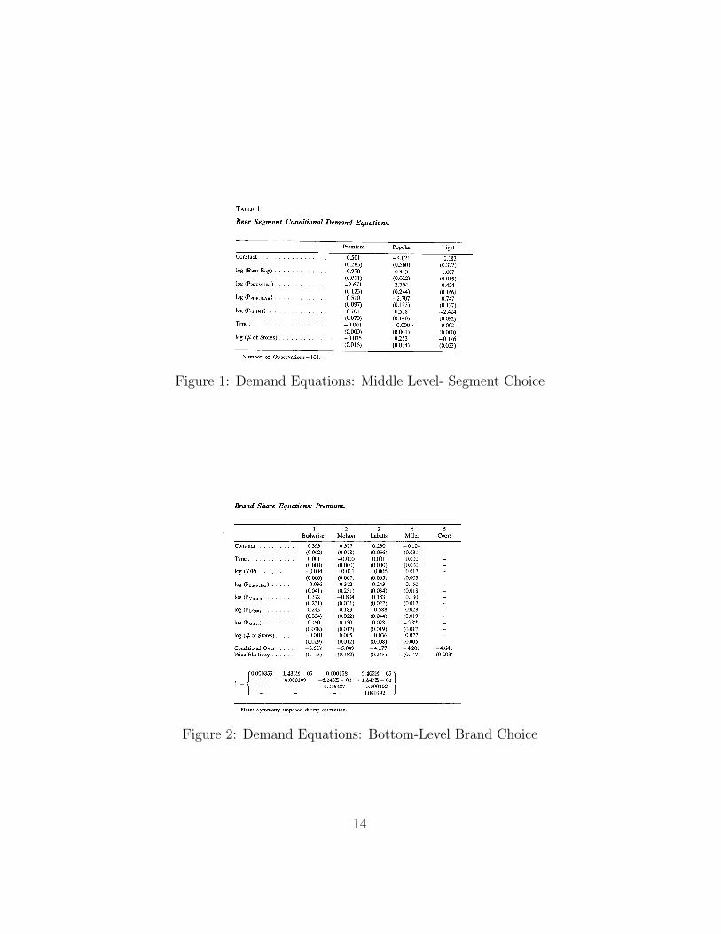
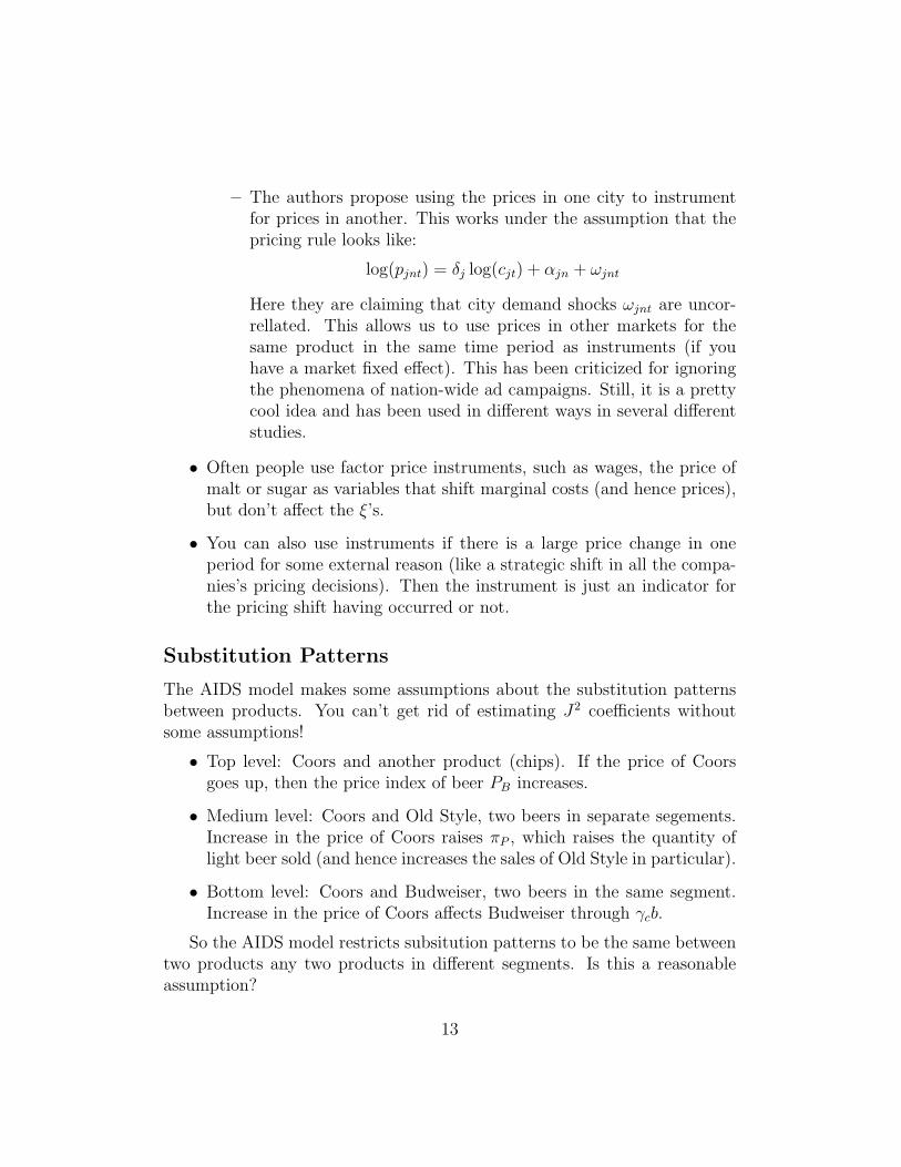
Figure 1: Demand Equations: Middle Level- Segment Choice

Figure 2: Demand Equations: Bottom-Level Brand Choice

14

Figure 3: Segment Elasticities

Figure 4: Overall Elasticities

15

Chaudhuri, Goldberg and Jia Paper

Question: The WTO has imposed rules on patent protection (both durationand enforcement) on member countries. There is a large debate on should weallow foreign multinationals to extent their drugs patents in poor countriessuch as India, which would raise prices considerably.

• Increase in IP rights raises the profits of patented drug firms, givingthem greater incentives to innovate and create new drugs (or formula-tions such as long shelf life which could be quite usefull in a countrylike India).

• Lower consumer surplus dues to generic drugs being taken off the mar-ket.

To understand the tradeoff inherent in patent protection, we need toestimate the magnitude of these two effects. This is what CGJ do.

Market

• Indian Market for antibiotics.

• Foreign and Domestic, Licensed and Non-Licensed producers.

• Different types of Antibiotics, in particular CGJ look at a particularclass: Quinolones.

• Different brands, packages, dosages etc...

• Question: What would prices and quantities look like if there were nounlicensed firms selling this product in the market? 1

Data

• The Data come from a market research firm. This is often the casefor demand data since the firms in this market are willing to pay largeamounts of money to track how well they are doing with respect to

1One of the reasons I.O. economists use structural models is that there is often noexperiment in the data, i.e. a case where some markets have this regulation and othersdon’t.

16

their competitors. However, prying data from these guys when theysell it for 10 000 a month to firms in the industry involves a lot of workand emailing.

• Monthly sales data for 4 regions, by product (down to the SKU level)and prices.

• The data come from audits of pharmacies, i.e. people go to a sampleof pharmacies and collect the data.

• Problem for the AIDS model: Over 300 different products, i.e. 90 000cross product interaction terms to estimate! CGJ need to do someserious aggregating of products to get rid of this problem: they willaggregate products by therapeutic class into 4 of these, interacted withthe nationality of the producer (not if they are licensed or not!).

• Some products enter and exit the sample. How can the AIDS modeldeal with this?

• Some products have different dosages than others. How does one con-struct quantity for this market.

Results

• CGJ estimate the AIDS specification with the aggregation of differentbrands to product level.

• You can get upper and lower bounds on marginal costs by assumingeither that firms are perfect competitors within the segment (i.e. p =mc) or by assuming that firms are operating a cartel which can price atthe monopoly level (i.e. p = mc

1+1/ηjj. This is very smart: you just get

a worse case scenario and show that even in the case with the highestpossible producer profits, these profits are small compared to the lossin consumer surplus. Often it is better to bound the bias from someestimates rather than attempt to solve the problem.

• Use estimated demand system to compute the prices of domestic pro-ducers of unlicensed products that make expenditures on these products0 (this is what “virtual prices” mean).

17

• Figure out what producer profits would be in the world without unli-censed firms (just (p− c)q in this setup).

• Compute the change in consumer surplus (think of integrating underthe demand curve).

18

antiinfectives segment ranks second in India,whereas in the world market it is fifth and has ashare of only 9.0 percent. Hence, antiinfectivesare important in India not only from a health

and public policy point of view, but also as asource of firm revenue.

With this in mind, we focus on one partic-ular subsegment of antiinfectives, namely the

TABLE 3—SUMMARY STATISTICS FOR THE QUINOLONES SUBSEGMENT: 1999–2000

North East West South

Annual quinolones expenditure per household (Rs.) 31.25 19.75 27.64 23.59(3.66) (3.67) (4.07) (2.86)

Annual antibiotics expenditure per household (Rs.) 119.88 84.24 110.52 96.24(12.24) (12.24) (9.60) (9.96)

No. of SKUsForeign ciprofloxacin 12.38 11.29 13.08 12.46

(1.50) (1.90) (1.02) (1.06)Foreign norfloxacin 1.83 1.71 2.00 1.58

(0.70) (0.75) (0.88) (0.83)Foreign ofloxacin 3.04 2.96 2.96 3.00

(0.86) (0.86) (0.91) (0.88)Domestic ciprofloxacin 106.21 97.63 103.42 105.50

(5.99) (4.34) (7.22) (4.51)Domestic norfloxacin 38.96 34.96 36.17 39.42

(2.71) (2.68) (2.51) (3.79)Domestic ofloxacin 18.46 16.00 17.25 17.25

(6.80) (6.34) (5.86) (6.35)Domestic sparfloxacin 29.83 28.29 31.21 29.29

(5.57) (6.38) (6.88) (6.57)Price per-unit API* (Rs.)

Foreign ciprofloxacin 9.58 10.90 10.85 10.07(1.28) (0.66) (0.71) (0.58)

Foreign norfloxacin 5.63 5.09 6.05 4.35(0.77) (1.33) (1.39) (1.47)

Foreign ofloxacin 109.46 109.43 108.86 106.12(6.20) (6.64) (7.00) (11.40)

Domestic ciprofloxacin 11.43 10.67 11.31 11.52(0.16) (0.15) (0.17) (0.13)

Domestic norfloxacin 9.51 9.07 8.88 8.73(0.24) (0.35) (0.37) (0.20)

Domestic ofloxacin 91.63 89.64 85.65 93.41(16.15) (15.65) (14.22) (14.07)

Domestic sparfloxacin 79.72 78.49 76.88 80.28(9.76) (10.14) (11.85) (10.37)

Annual sales (Rs. mill)Foreign ciprofloxacin 41.79 24.31 45.20 29.47

(15.34) (8.16) (12.73) (6.48)Foreign norfloxacin 1.28 1.00 0.58 0.73

(1.01) (0.82) (0.44) (0.57)Foreign ofloxacin 54.46 31.84 35.22 31.11

(13.99) (9.33) (9.06) (7.03)Domestic ciprofloxacin 962.29 585.91 678.74 703.81

(106.26) (130.26) (122.26) (87.40)Domestic norfloxacin 222.55 119.71 149.18 158.29

(38.84) (19.45) (26.91) (16.26)Domestic ofloxacin 125.02 96.21 149.36 112.05

(44.34) (30.11) (52.82) (42.59)Domestic sparfloxacin 156.17 121.75 161.30 98.11

(31.41) (25.76) (46.74) (34.20)

Note: Standard deviations in parentheses.* API: Active pharmaceutical ingredient.

1483VOL. 96 NO. 5 CHAUDHURI ET AL.: GLOBAL PATENT PROTECTION IN PHARMACEUTICALS

Figure 5: Summary Statistics

19

foreign product is in stock), in aggregate datawe would expect to find precisely the substitu-tion patterns that we report in Table 6.

Whether the particular explanation we provideabove is the correct one, the high degree of sub-stitutability between domestic product groupsturns out to have important implications for thewelfare calculations. We discuss these in moredetail below when we present the results of thecounterfactual welfare analysis. Another elasticitywith important implications for the counterfactu-als is the price elasticity for the quinolone subseg-ment as a whole, which indicates how likelyconsumers are to switch to other antibioticsgroups, when faced with a price increase for quin-olones. This elasticity is computed on the basis ofthe results in Table A3, and it is at 1.11 (stan-dard error: 0.24); this is large in magnitude,but—as expected—smaller in absolute value thanthe own-price elasticities of the product groupswithin the quinolone subsegment.

The results in Tables 6A and 6B are based onour preferred specification discussed in SectionII. In Tables A4 to A6 in the Appendix, weexperiment with some alternative specifications.Tables A4(a)–A4(c) correspond to a specificationthat includes, in addition to product-group-specificregional fixed effects, product-group-specific (andfor the upper level antibiotics-segment-specific)seasonal effects. We distinguish among three sea-sons—the summer, monsoon, and winter—andreport the unconditional demand elasticities for

the northern region for each of these seasons. Asevident from the tables in the Appendix, our elas-ticity estimates are robust to the inclusion of sea-sonal effects. The demand elasticities in Table A5are based on estimation of the demand system byOLS. Compared to the elasticities obtained by IV,the OLS elasticities are smaller in absolute value,implying that welfare calculations based on theOLS estimates would produce larger welfare lossestimates. Nevertheless, some of the patterns re-garding the cross-price elasticities discussed ear-lier are also evident in the OLS results; inparticular, the cross-price elasticities between dif-ferent domestic product groups are all positive,large, and significant, and in most instances largerthan the cross-price elasticities between drugs thatcontain the same molecule but are produced byfirms of different domestic/foreign status. Theclose substitutability of domestic products indi-cated by both the OLS and IV estimates seems tobe one of the most robust findings of the paper.

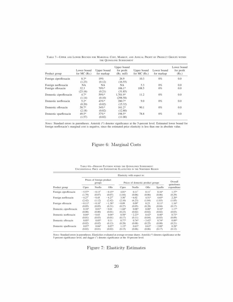
B. Cost and Markup Estimates

Table 7 displays the marginal costs, markups,and profits implied by the price elasticity esti-mates of Tables 6A and 6B for each of the sevenproduct groups. Given that our regional effectsimply different price elasticities for each region,our marginal cost and markup estimates alsodiffer by region. Given, however, that based on

TABLE 7—UPPER AND LOWER BOUNDS FOR MARGINAL COST, MARKUP, AND ANNUAL PROFIT BY PRODUCT GROUPS WITHIN

THE QUINOLONE SUBSEGMENT

Product groupLower boundfor MC (Rs.)

Upper boundfor markup

Upper boundfor profit(Rs. mill)

Upper boundfor MC (Rs.)

Lower boundfor markup

Lower boundfor profit

(Rs.)

Foreign ciprofloxacin 8.3* 19% 26.9 10.3 0% 0.0(1.23) (0.12) (16.55)

Foreign norfloxacin NA NA NA 5.3 0% 0.0Foreign ofloxacin 32.3 70%* 106.1* 108.5 0% 0.0

(23.16) (0.21) (31.85)Domestic ciprofloxacin 4.7* 59%* 1,701.9* 11.2 0% 0.0

(1.14) (0.10) (298.58)Domestic norfloxacin 5.2* 43%* 280.7* 9.0 0% 0.0

(0.20) (0.02) (15.32)Domestic ofloxacin 58.7* 34%* 161.2* 90.1 0% 0.0

(2.18) (0.02) (12.80)Domestic sparfloxacin 49.5* 37%* 198.5* 78.8 0% 0.0

(1.57) (0.02) (11.00)

Notes: Standard errors in parentheses. Asterisk (*) denotes significance at the 5-percent level. Estimated lower bound forforeign norfloxacin’s marginal cost is negative, since the estimated price elasticity is less than one in absolute value.

1500 THE AMERICAN ECONOMIC REVIEW DECEMBER 2006

Figure 6: Marginal Costs

not impose it through any of our assumptionsregarding the demand function. The questionthat naturally arises, then, is what might explainthis finding. While we cannot formally addressthis question, anecdotal accounts in various in-dustry studies suggest that the explanation maylie in the differences between domestic andforeign firms in the structure and coverage ofretail distribution networks.

Distribution networks for pharmaceuticals inIndia are typically organized in a hierarchicalfashion. Pharmaceutical companies deal mainlywith carrying and forwarding (C&F) agents, inmany instances regionally based, who each sup-ply a network of stockists (wholesalers). Thesestockists, in turn, deal with the retail pharma-cists through whom retail sales ultimately oc-cur.35 The market share enjoyed by a particularpharmaceutical product therefore depends inpart on the number of retail pharmacists who

stock the product. And it is here that thereappears to be a distinction between domesticfirms and multinational subsidiaries. In particu-lar, the retail reach of domestic firms, as agroup, tends to be much more comprehensivethan that of multinational subsidiaries (IndianCredit Rating Agency (ICRA), 1999).36

There appear to be two reasons for this. Thefirst is that many of the larger Indian firms,because they have a much larger portfolio ofproducts over which to spread the associatedfixed costs, typically have more extensive net-works of medical representatives. The second issimply that there are many more domestic firms(and products) on the market. At the retail level,this would imply that local pharmacists mightbe more likely to stock domestic products con-taining two different molecules, say ciprofloxa-cin and norfloxacin, than they would domesticand foreign versions of the same molecule. Tothe extent that patients (or their doctors) arewilling to substitute across molecules in order tosave on transport or search costs (e.g., going toanother pharmacy to check whether a particular

35 There are estimated to be some 300,000 retail pharma-cists in India. On average, stockists deal with about 75 retailers(ICRA, 1999). There are naturally variations in this structure,and a host of specific exclusive dealing and other arrangementsexists in practice. Pharmaceutical firms also maintain networksof medical representatives whose main function is to marketthe company’s products to doctors who do the actual prescrib-ing of drugs. In some instances, firms do sell directly to thedoctors who then become the “retailer” as far as patients areconcerned, but these are relatively rare.

36 These differences were also highlighted in conversa-tions one of the authors had with CEOs and managingdirectors of several pharmaceutical firms, as part of a sep-arate study.

TABLE 6A—DEMAND PATTERNS WITHIN THE QUINOLONES SUBSEGMENT:UNCONDITIONAL PRICE AND EXPENDITURE ELASTICITIES IN THE NORTHERN REGION

Product group

Elasticity with respect to:

Prices of foreign productgroups Prices of domestic product groups Overall

quinolonesexpenditureCipro Norflo Oflo Cipro Norflo Oflo Sparflo

Foreign ciprofloxacin 5.57* 0.13† 0.15* 4.01* 0.11† 0.11† 0.16* 1.37*(1.79) (0.07) (0.07) (1.84) (0.06) (0.06) (0.06) (0.29)

Foreign norfloxacin 4.27† 0.45 4.27† 3.50† 6.02 4.51* 4.65* 2.20*(2.42) (1.12) (2.42) (2.10) (6.23) (1.84) (1.83) (1.05)

Foreign ofloxacin 0.11* 0.10† 1.38* 0.09 0.09† 0.23 0.11* 1.16*(0.05) (0.05) (0.31) (0.27) (0.05) (0.28) (0.04) (0.17)

Domestic ciprofloxacin 0.18* 0.01* 0.01 1.68* 0.08* 0.08* 0.10* 1.17*(0.08) (0.00) (0.01) (0.23) (0.02) (0.02) (0.02) (0.03)

Domestic norfloxacin 0.04* 0.03 0.04* 0.58* 2.23* 0.42* 0.40* 0.73*(0.01) (0.03) (0.01) (0.17) (0.11) (0.04) (0.03) (0.09)

Domestic ofloxacin 0.05* 0.05* 0.11 0.77* 0.74* 3.42* 0.74* 0.89*(0.02) (0.02) (0.13) (0.28) (0.08) (0.25) (0.08) (0.21)

Domestic sparfloxacin 0.07* 0.04* 0.07* 1.15* 0.63* 0.63* 2.88* 0.28*(0.02) (0.01) (0.02) (0.15) (0.06) (0.06) (0.17) (0.12)

Notes: Standard errors in parentheses. Elasticities evaluated at average revenue shares. Asterisk (*) denotes significance at the5-percent significance level, and dagger (†) denotes significance at the 10-percent level.

1498 THE AMERICAN ECONOMIC REVIEW DECEMBER 2006

Figure 7: Elasticity Estimates

20

Characteristic Space Approaches to Demand

Estimation

Basic approach:

• Consider products as bundles of characteristics

• Define consumer preferences over characteristics

• Let each consumer choose that bundle which maximizes their utility.We restrict the consumer to choosing only one bundle. You will see whywe do this as we develop the formal model, multiple purchases are easyto incorporate conceptually but incur a big computational cost andrequire more detailed data than we usually have. Working on elegantways around this problem is an open area for research.

• Since we normally have aggregate demand data we get the aggregatedemand implied by the model by summing over the consumers.

Formal Treatment

• Utility of the individual:

Uij = U (xj, pj, vi; θ)

for j = 0, 1, 2, 3, ..., J .

• Good 0 is generally referred to as the outside good. It represents the op-tion chosen when none of the observed goods are chosen. A maintainedassumption is that the pricing of the outside good is set exogenously.

• J is the number of goods in the industry

• xj are non-price characteristics of good j

• pj is the price

• vi are characteristics of the consumer i

• θ are the parameters of the model

21

• Note that the product characteristics do not vary over consumers, thismost commonly a problem when the choice sets of consumers are dif-ferent and we do not observe the differences in the choice sets.

• Consumer i chooses good j when

Uij > Uik ∀k [note that all preference relations are assumed to be strict](4)

• This means that the set of consumers that choose good j is given by

Sj (θ) = v|Uij > Uik ∀k

and given a distribution over the v’s, f (v) , we can recover the shareof good j as

sj (x,p|θ) =

∫ν∈Sj(θ)

f (dν)

Obviously, if we let the market size be M then the total demand issj (x,p|θ) .

• This is the formal analog of the basic approach outlined above. The restof our discussion of the characteristic space approach to demand willconsider the steps involved in making this operational for the purposesof estimation.

Aside on utility functions

• Recall from basic micro that ordinal rankings of choices are invari-ant to affine transformations of the underlying utility function. Morespecifically, choices are invariant to multiplication of U (·) by a positivenumber and the addition of any constant.

• This means that in modelling utility we need to make some normaliza-tions - that is we need to bolt down a zero to measure things against.Normally we do the following:

1. Normalize the mean utility of the outside good to zero.

2. Normalize the coefficient on the idiosyncratic error term to 1.

This allows us the interpret our coefficients and do estimation.

22

Examples

Anderson, de Palma and Thisse go through many of these in very closedetail...

Horozontally Differentiated vs Vertically Differentiated - Horo-zontally differentiated means that, setting aside price, people dissagree overwhich product is best. Vertically differentiated means that, price aside, ev-eryone agrees on which good is best, they just differ in how much they valueadditional quality.

1. Pure Horizontal Model

• – This is the Hotelling model (n icecream sellers on the beach,with consumers distributed along the beach)

– Utility for a consumer at some point captured by νi is

Uij = u− pj + θ (δj − νi)2

where the (δj − νi)2 term captures a quadratic ”transporta-

tion cost”.

– It is a standard workhorse for theory models exploring ideasto do with product location.

2. Pure Vertical Model

• – Used by, Shaked and Sutton, Mussa-Rosen (monopoly pric-ing, slightly different), Bresnahan (demand for autos) andmany others

– Utility given byUij = u− νipj + δj

– This model is used most commonly in screening problemssuch a Mussa-Rosen where the problem is to set (p, q) tu-ples that induce high value and low value customers to self-select (2nd degree price discrimination). The model has alsobeen used to consider product development issues, notablyin computational work.

23

3. Logit

• – This model assumes everyone has the same taste for qualitybut have different idiosyncratic taste for the product. Utilityis given by

Uij = δj + εij

– εijiid∼ extreme value type II [F (ε) = e− e−ε]. This is a very

helpful assumption as it allows for the aggregate shares tohave an analytical form.

– This ease in aggregation comes at a cost, the embedded as-sumption on the distribution on tastes creates more struc-ture than we would like on the aggregate substitution ma-trix.

– See McFadden 1972 for details on the construction.

4. Nested Logit

• As in the AIDS Model, we need to make some “ex-ante” classifi-cation of goods into different segments, so each good j ∈ S(j).

• Probabilities are given by:

F (·) = exp(−S∑

s=1

(∑

j∈S(j)

e−εnj/λk)λk)

For two different goods in different segments, the relative choiceprobabilities are:

Pni

Pnm

=eVni λk(

∑j∈Sk(i) e

Vnj λkλk−1

eVnm λl(∑

j∈Sl(m) eVnj λlλl−1

• The best example of using Nested-Logit for an IO application isGolberg (1995) Econometrica (in the same issue as BLP on thesame industry!).

• One can classify goods into a hierarchy of nests (car or truck,foreign or domestic, nissan or toyota, camry or corrola).

24

5. “Generalized Extreme Value Models”: Bresnahan, Trajtenberg andStern (RAND 1997) have looked at extensions of nested logit whichallow for overlapping nests: foreign or domestic computer maker in onenest and high-end or standard performance level. The advantage ofthis approach is that there is no nead to choose which nest comes first.

6. Ken Train (2002) discusses many different models of discrete choice.This is a great reference to get into the details of how to do theseprocedures. Moreover we will focus on cases where we have aggregatedata, but having individual level data can help you A LOT.

7. ”Ideal Type” (ADT) or ”Pure Characteristic” (Berry & Pakes)

• – Utility given by

Uij = f (νi, pj) +∑

k

∑r

g (xjk, νir, θkr)

This nests the pure horizontal and pure vertical models (onceyou make a few function form assumptions and some nor-malizations.

8. BLP (1996)

• – This is a parameterized version of the above case, with thelogit error term tacked on. It is probably the most com-monly used demand model in the empirical literature, whendifferentiated goods are being dealt with.

Uij = f (νi, pj) +∑

k

∑r

xjkνirθkr + εij

Estimation from Product Level Aggregate Data

• The data typically are shares, prices and characteristics

• That is: (sj, pj, xj)Jj=1

• We will start by looking at the simpler cases (the vertical model andthe logit) and then move onto an examination of BLP.

• Remember that all the standard problems, like price being endogenousand wider issues of identification, will continue to be a problem here.So don’t lose sight of this in all the fancy modelling!

25

Illustrative Case: Vertical Model

Note that this is what Bresnahan estimates when he looks at the possibilityof collusion explaining the relative dip in auto prices in 1955.

1. In the vertical model people agree on the relative quality of products,hence there is a clear ranking of products in terms of quality

2. The only difference between people is that some have less willingnessto pay for quality than others

3. Hence (recall) utility will look like

Uij = u− νipj + δj

4. To gain the shares predicted by the model we need to

5. Order the goods by increasing p. Note that this requires the orderingto also be increasing in δ if the goods in the sample all have non-zeroshare. (A good with higher p and lower δ will not be purchased byanyone.)

6. The lowest good is the outside good (good 0) - we normalise this tozero (u = 0)

7. Choose 0 if

0 > maxj≥1

(δj − νipj)

this implies νi >δ1p1

8. Hence S0 =ν∣∣∣ν > δ1

p1

. Thus if ν is distributed lognormally, ν =

exp (σx+ µ) where x is distributed standard normal, then choose 0 if

exp (σx+ µ) ≥ δ1p1

or ν ≥ ψ0 (θ)

where ψ0 (θ) ≡ σ−1[log(

δ1p1

)− µ

], that is our model has s0 = F (ψ0 (θ)) ,

where F is standard normal

26

9. Similarly, choose good 1 iff 0 < δ1 − νp1 and δ1 − νp1 ≥ δ2 − νp2, or:

s1 (θ) = F (ψ1 (θ))− F (ψ0 (θ))

more generally

sj (θ) = F (ψj (θ))− F (ψj−1 (θ))

for j = 1, ...J .

10. Question: What parameters are identified in θ? What are the sourcesof identification for each parameter?

Estimation To complete estimation we need to specify a data generat-ing process. We assume we observe the choices of a random sample of sizen. Each individual chooses one from a finite number of cells; Choices aremutually exclusive and exhaustive.This suggests a multinomial distribution of outcomes

Lj ∝ Πjsj (θ)nj

Hence, choose θ to maximise the log-likelihood

maxθ

n∑

j

s0j log [sj (θ)]

Where nj is the count of individuals choosing the object.

Another Example: Logit

sj =exp [δj − pj]

1 +∑

q≥1 exp [δq − pq]

s0 =1

1 +∑

q≥1 exp [δq − pq]

Here the utility isUij = δj + εij

1. • – εijiid∼ extreme value type II [F (ε) = e− e−ε].

27

Identification:

Identification is the key issue, always. Here we have to get all the identi-fication off the shares. Since s0 = 1 −

∑j≥1 sj we have J shares to use to

identify J+2 parameters (if we let θ = δ1, ..., δJ , µ, σ). (you should be ableto explain this with a simple diagram) Thus hit the dimensionality problem.To solve this we need more structure. Typically we reduce the dimensionalityby ”projecting” product quality down onto characteristics, so that:

δj =∑

k

βkxkj

This makes life a lot easier and we can now estimate via MLE.An alternative approach would have been to use data from different re-

gions or time periods which would help with this curse of dimensionality.Note that we are still in much better shape that the AIDS model since thereare only J + 2 parameters to estimate versus J2 + J of them.

Problems with Estimates from Simple Models:

Each model has its own problems and they share one problem in common:

• Vertical Model:

1. Cross-price elasticities are only with respect to neighbouring goods- highly constrained substitution matrix.

2. Own-price elasticities are often not smaller for high priced goods,even though we might think this makes more sense (higher income→ less price sensitivity).

• Logit Model:

1. Own price derivative is ∂s∂p

= −s (1− s) . That is, the own pricederivative only depends on shares, which in turn means that if wesee two products with the same share, they must have the samemark-up, under most pricing models.

28

2. Cross-price elasticities are sjsk. This means that the substitutionmatrix is solely a function of shares and not relative proximity ofproducts in characteristic space. This is a bit crazy for productslike cars. This is a function of the IIA assumption.

– Note: if you run logit, and your results do not generate theseresults you have bad code. This is a helpful diagnostic for pro-gramming.

• Simultaneity: No way to control for endogeniety via simultaneity. Thisleads to the same economically stupid results that we see in single prod-uct demand estimation that ignores endogeniety (like upward slopingdemand etc).

Dealing with Simultaneity

The problem formally is that the regressors are correlated with an unob-servable (we can’t separate variation due to cost shocks from variationdueto demand shocks), so to deal with this we need to have an unobservablecomponent in the model.Let product quality be

δj =∑

k

βkxkj − αp+ ξj

Where the elements of ξ are unobserved product characteristics

Estimation Strategy

1. Assume n large

2. So soj = sj (ξ1, ..., ξJ |θ)

3. For each θ there exists a ξ such that the model shares and observedshares are equal.

4. Thus we invert the model to find ξ as a function of the parameters.

5. This allows us to construct moments to drive estimation (we are goingto run everything using GMM)

• Note: sometimes inversion is easy, sometimes it is a real pain.

29

Example: The Logit Model Logit is the easiest inversion to do, since

ln [sj]− ln [s0] = δj =∑

k

βkxkj − αp+ ξj

ξj = ln [sj]− ln [s0]−

(∑k

βkxkj − αp+ ξj

)• – Note that as far as estimation goes, we now are in a linear world

where we can run things in the same way as we run OLS or IVor whatever. The precise routine to run will depend, as always,on what we think are the properties of ξ.

– Further simple examples in Berry 1994

More on Estimation

• Regardless of the model we now have to choose the moment restrictionwe are going to use for estimation.

• This is where we can now properly deal with simultaneity in our model.

• Since consumers know ξj we should probably assume the firms do aswell. Thus in standard pricing models you will have

pj = p (xj, ξj, x−j, ξ−j)

• Since p is a function of the unobservable, ξ, we should not use a momentrestriction which interacts p and ξ. This is the standard endogenietyproblem in demand estimation.

• It implies we need some instruments.

• There is nothing special about p in this context, if E (ξx) 6= 0, then weneed an instruments for x as well.

Some assumptions used for identification in literature:

1. E (ξ|x,w) = 0 x contains the vector of characteristics other than priceand w contains cost side variables. Note that they are all valid instru-ments for price so long as the structure of the model implies they arecorrelated with pj.

Question: how do the vertical and logit models differ in this regard?

30

2. Multiple markets: here assume something like

ξjr = ξj + ujr

and put assumptions on ujr. Essentially treat the problem as a paneldata problem, with the panel across region not time.

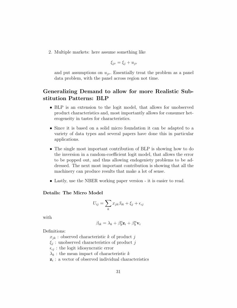
Generalizing Demand to allow for more Realistic Sub-stitution Patterns: BLP

• BLP is an extension to the logit model, that allows for unobservedproduct characteristics and, most importantly allows for consumer het-erogeneity in tastes for characteristics.

• Since it is based on a solid micro foundation it can be adapted to avariety of data types and several papers have done this in particularapplications.

• The single most important contribution of BLP is showing how to dothe inversion in a random-coefficient logit model, that allows the errorto be popped out, and thus allowing endogeniety problems to be ad-dressed. The next most important contribution is showing that all themachinery can produce results that make a lot of sense.

• Lastly, use the NBER working paper version - it is easier to read.

Details: The Micro Model

Uij =∑

k

xjkβik + ξj + ειj

withβik = λk + βo

kzi + βukvi

Definitions:xjk : observed characteristic k of product jξj : unobserved characteristics of product jειj : the logit idiosyncratic errorλk : the mean impact of characteristic kzi : a vector of observed individual characteristics

31

βok : a vector of coefficients determining the impact of the elements of zi

on the taste for characteristic xjk

vi : a vector of unobserved individual characteristicsβu

k : a vector of coefficients determining the impact of the elements of vi

on the taste for characteristic xjk

• Substituting the definition of βik into the utility function you get

Uij =∑

k

xjkλk +∑

k

xjkβokzi +

∑k

xjkβukvi + ξj + ειj

or, as is usually the way this is written (and also the way you end upthinking about things when you code up the resulting estimator)

Uij = δj +∑

k

xjkβokzi +

∑k

xjkβukvi + ειj

whereδj =

∑k

xjkλk + ξj

• Note that this model has two different types of interactions betweenconsumer characteristics and product characteristics:

1. (a) i. Interactions between observed consumer characteristics zi

and product characteristics xjk’s; and

ii. Interactions between unobserved consumer characteristics vi

and product characteristics xjk’s

• These interactions are the key things in terms of why this model isdifferent and preferred to the logit model. These interactions kill theIIA problem and mean that the aggregate substitution patterns arenow far more reasonable (which is to say they are not constrained tohave the logit form).

– Question: Are the substitution patterns at the individual levelany different from the logit model?

The intuition for why things are better now runs as follows:

32

Figure 1: The Reliant Regal

• Thus they will substitute to cars that are close to the BMW in characteristic space

(say a Lexus, and not a Reliant Regal (a three wheeled engineering horror story still

sometimes seen in the UK)

• Also, price effects will be different for different products. Products with high prices,but low shares, will be bought by people who don’t respond much to price and so they

will likely have higher markup than a cheap product with the same share.

• This model also means that products can be either strategic complements or substitutesin the pricing game. (in Logit they are strategic complements).

• Usually, we only have product level data at the aggregate level so the source of consumerinformation is the distribution of zi from the census. That is, we are usually working

with the vi part of the model. However, a few studies have used micro data of one

form or another, notably MicroBLP (JPE 2004).

• With micro data you need to think about whether the individual specific data you haveis enough to capture the richness of choices. If not, then you need to also include the

unobserved part of the model as well.

20

Figure 8: The Reliant Regal

• If the price of product j (say a BMW 7 series) increases, very specificcustomers will leave the car - those customers who have a preferencefor the car’s characteristics and consequently will like cars close to itin the characteristic space that the empirical researcher is using.

• Thus they will substitute to cars that are close to the BMW in charac-teristic space (say a Lexus, and not a Reliant Regal (a three wheeledengineering horror story still sometimes seen in the UK)

• Also, price effects will be different for different products. Products withhigh prices, but low shares, will be bought by people who don’t respondmuch to price and so they will likely have higher markup than a cheapproduct with the same share.

• This model also means that products can be either strategic comple-

33

ments or substitutes in the pricing game. (in Logit they are strategiccomplements).

• Usually, we only have product level data at the aggregate level so thesource of consumer information is the distribution of zi from the census.That is, we are usually working with the vi part of the model. However,a few studies have used micro data of one form or another, notablyMicroBLP (JPE 2004).

• With micro data you need to think about whether the individual spe-cific data you have is enough to capture the richness of choices. Ifnot,then you need to also include the unobserved part of the model aswell.

Estimation: Step by step overview

We consider product level data (so there are no observed consumer charac-teristics). Thus we only have to deal with the v’sStep 1: Work out the aggregate shares conditional on (δ, β)

• After integrating out the ειj (recall that these are familiar logit errors)the equation for the share is

sj (δ, β) =

∫exp [δj +

∑k xjkviβk]

1 +∑

q≥1 exp [δq +∑

k xqkviβk]f (v) dv

• This integral is not able to be solved analytically. (compare to thelogit case). However, for the purposes of estimation we can handlethis via simulation methods. That is, we can evaluate the integral usecomputational methods to implement an estimator...

• Take ns simulation draws from f (v). This gives you the simulatedanalog

snsj (δ, β) =

∑r

exp [δj +∑

k xjkvirβk]

1 +∑

q≥1 exp [δq +∑

k xqkvirβk]

Note the following points:

• The logit error is very useful as it allows use to gain some precision insimulation at low cost.

34

• If the distribution of a characteristic is known from Census data thenwe can draw from that distribution (BLP fits a Lognormal to censusincome data and draws from that)

• By using simulation you introduce a new source of error into the es-timation routine (which goes away if you have “enough” simulationsdraws...). Working out what is enough is able to be evaluated (seeBLP). The moments that you construct from the simulation will ac-count for the simulation error without doing special tricks so this ismainly a point for interpreting standard errors.

• The are lots of ways to use simulation to evaluate integrals, some ofthem are quite involved. Depending on the computational demands ofyour problem it could be worth investing some time in learning someof these methods. (Ken Judd has a book in computation methods ineconomics that is a good starting point, Ali can also talk to you aboutusing an extension of Halton Draws, called the Latin Cube to performthis task)

Step 2: Recover the ξ from the shares.Remember from basic econometrics that when we want to estimate using

GMM we want to exploit the orthogonality conditions that we impose on thedata. To do this we need to be able to compute the unobservable, so as toevaluate the sample moments.

[Quickly review OLS as reminder]Recall that

δj =∑

k

xjkλk + ξj

so, once we know δj we can run this regression as OLS or IV or whateverand get the ξj. Then we can construct the moments for the estimator.

So how to do this? This is the bit where BLP does something very cool.

• BLP point out that iterating on the system

δkj (β) = δk−1

j (β) + ln[so

j

]− ln

[sns

j

(δk−1, β

)]has a unique solution (the system is a contraction mapping with mod-ulus less than one and so has a fixed point to which it converges mono-tonically at a geometric rate). Neither, Nevo or BLP point this out,

35

although both exploit it, but the following is also a contraction

exp[δkj (β)

]= exp

[δk−1j (β)

] soj

snsj (δk−1, β)

This is what people actually use in the programming of the estimator.

• So given we have δ (β, so, P ns) we have an analytical form for λ andξ (which we be determined by the exact indentifying assumptions youare using). In other words

ξ (β, so, P ns) = δ (β, so, P ns)−∑

k

xkλk

• The implication is that you should only be doing a nonlinear searchover the elements of β.

Step 3: Construct the MomentsWe want to interact ξ (β, so, P ns) with the instruments which will be the

exogenous elements of x and our instrumental variables w (recall that we willbe instrumenting for price etc).

You need to make sure that you have enough moment restrictions toidentify the parameters of interest.

In evaluating the moment restrictions we impose a norm which will usu-ally be the L2 norm. ie

‖GJ,ns‖2 =

√∑j

[ξjfj (x,w)]2

Step 4: Iterate until have reached a minimum

• Recall that we want to estimate (λ, β) . Given the β the λ have analyticform, we only need to search over the β that minimize our objectivefunction for minimizing the moment restrictions.

• Look back at the expression for the share and you will realize that theβ is the only thing in there that we need to determine to do the restof these steps. However, since it enters nonlinearly we need to do anonlinear search to recover the values of β that minimize our objectivefunction over the moments restrictions. Nevo uses the difference be-tween linear and non-linear parameters to estimate brand fixed-effects(and I’ve done brand/market fixed effects too).

36

• You will need to decide on a stopping point.

• Some things to note about this:

– This means that estimation is computationally intensive.

– You will need to use Matlab, Fortran, C, Guass etc to code it up.I like Matlab, personally.

– There are different ways to numerically search for minimums:always prefer use a simplex search algorithm over derivative basedmethods, simplex searches take a little longer but are more robustto poorly behaved functions. Also start you code from severaldifferent places before believing a given set of results. [in matlabfminsearch is a good tool].

– Alternatively, and even better thing to do is to use a program thatcan search for global minima so that you don’t have to worry toomuch about starting values. These can take about 10-20 timeslonger, but at least you can trust your estimates. My favoriteminimizers are Differential Evolution and Simulated Annealing.You can get these in MATLAB, C or FORTRAN off the web.

– Aviv Nevo has sample code posted on the web and this is a veryuseful place to look to see the various tricks in programming thisestimator.

– Due to the non-linear nature of the estimator, the computationof the standard errors can be a arduous process, particularly ifthe data structure is complex.

– Taking numerical derivatives will often help you out in the com-putation of standard errors.

– For more details on how to construct simulation estimators andthe standard errors for nonlinear estimators, look to you econo-metrics classes...

37

Identification in these models

The sources of identification in the standard set up are going be:

1. differences in choice sets across time or markets (i.e. changes in char-acteristics like price, and the other x’s)

2. differences in underlying preferences (and hence choices) over time oracross markets

3. observed differences in the distribution of consumer characteristics (likeincome) across markets

4. the functional form will play a role (although this is common to anymodel, and it is not overly strong here)

• so if you are especially interesting in recovering the entire distributionof preferences from aggregate data you may be able to do it with suf-ficiently rich data, but it will likely be tough without some additionalinformation or structure.

• additional sources of help can be:

– adding a pricing equation (this is what BLP does)

– add data, like micro data on consumer characteristics, impose ad-ditional moments from other data sources to help identify effectsof consumer characteristics (see Petrin on the introduction of theminivan), survey data on who purchases what (MicroBLP).

Nevo

• Nevo is trying to understand why there are such high markups in theReady-to-Eat Cereal Industry, and where does market power come fromin this industry.

• Part of the story comes from the production side: there are only 13plants in the U.S. that manufacture RTE cereal. Nevo will focus onthe demand side.

38

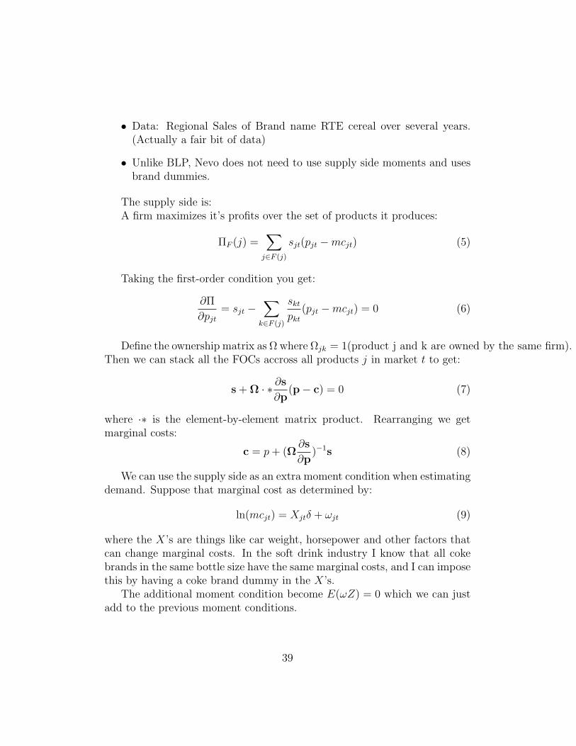
• Data: Regional Sales of Brand name RTE cereal over several years.(Actually a fair bit of data)

• Unlike BLP, Nevo does not need to use supply side moments and usesbrand dummies.

The supply side is:A firm maximizes it’s profits over the set of products it produces:

ΠF (j) =∑

j∈F (j)

sjt(pjt −mcjt) (5)

Taking the first-order condition you get:

∂Π

∂pjt

= sjt −∑

k∈F (j)

skt

pkt

(pjt −mcjt) = 0 (6)

Define the ownership matrix as Ω where Ωjk = 1(product j and k are owned by the same firm).Then we can stack all the FOCs accross all products j in market t to get:

s + Ω · ∗ ∂s∂p

(p− c) = 0 (7)

where ·∗ is the element-by-element matrix product. Rearranging we getmarginal costs:

c = p+ (Ω∂s

∂p)−1s (8)

We can use the supply side as an extra moment condition when estimatingdemand. Suppose that marginal cost as determined by:

ln(mcjt) = Xjtδ + ωjt (9)

where the X’s are things like car weight, horsepower and other factors thatcan change marginal costs. In the soft drink industry I know that all cokebrands in the same bottle size have the same marginal costs, and I can imposethis by having a coke brand dummy in the X’s.

The additional moment condition become E(ωZ) = 0 which we can justadd to the previous moment conditions.

39

AVIV NEVO

TABLE I11

DETAILED OF PRODUC~IONESTIMATES COSTS

% of Mfr % of Retail Item $/lb Price Price

Manufacturer Price Manufacturing Cost:

Grain Other Ingredients Packaging Labor Manufacturing Costs (net of capital costs)"

Gross Margin Marketing Expenses:

Advertising Consumer Promo (mfr coupons) Trade Promo (retail in-store)

Operating Profits

"apital costs were computed from ASM data. Soirrcr: Cotterill (1996) reporting from estimates in CS First Boston Reports "Kellogg Company."

New York, October 25, 1994.

(SIC 20). The gross price-average variable cost margin for the RTE cereal industry is 64.4%, compared to 26.5% for the aggregate food s e ~ t o r . ~ Accounting estimates of price-marginal cost margins taken from Cotterill (1996), presented in Table 111, are close to those above. Here the estimated gross margin is 7 percentage points lower than before, which can be attributed to the fact that these are marginal versus average costs. The last column of the table presents the retail margins.

3. THE EMPIRICAL FRAMEWORK

My general strategy is to consider different models of supply conduct. For each model of supply, the pricing decision depends on brand-level demand, which is modeled as a function of product characteristics and consumer prefer- ences. Demand parameters are estimated and used to compute the PCM implied by different models of conduct. I use additional information on costs to compute observed PCM and choose the conduct model that best fits these margins.

"he margins for the aggregate food sector are given only as support to the claim previously made that the margins of RTE cereal are "high." At this point no attempt has been made to explain these differences. As was pointed out in the Introduction, several explanations are possible. One of the goals of the analysis below will be to separate these possible explanations.

Figure 9: Costs and Back of the envellope markups in the RTE Cereal In-dustry.

40

327 MEASURING MARKET POWER

TABLE VI

RESULTSFROM THE FULLMODEL^

Standard Interaction? with Demographic Variables Means Deviations

Variablc ( p ' s ) (v 's) Incume Illcomc Sq Age Child

Price

Advertising

Constant

Cal from Fat

Sugar

Mushy

Fiber

All-family

Kids

Adults

GMM Objective (degrees of freedom) MD X 2

% of Price Coefficients > 0

"Based on 27,862 obrervations. Except where noted, parameters are GMM estimates. All regrersionr include brand and time dummy variables. Arymptotically robust rtandard errors are given in parentherer.

"stimater from a minimum-dirtance procedure.

regional prices in all quarters and the cost proxies discussed in the previous section. The results from the preferred specification are presented in Table VI. This specification does not include city fixed effects. I also examined a specifica- tion, equivalent to that presented in Table V column (x), which includes city specific intercepts. The point estimates are close to those of the preferred specification but the standard errors are very large, which is not surprising given that demographics are approximately constant during the sample period. Essen- tially the more elaborate manner in which the full model incorporates demo- graphics seems to fully control for city specific effects. Additional specifications are discussed and presented in Appendix B.

The means of the distribution of marginal utilities, P's, are estimated by a minimum-distance procedure described above and presented in the first column. All coefficients are statistically significant and basically of the expected sign. The ability of the observed characteristics to fit the coefficients of the brand dummy variables is measured by using the chi-squared test, described in Section 4.4, which is presented at the bottom of Table VI. Since the brand dummy variables

Figure 10: Estimated BLP Model.

41

MEASURING MARKET POWER

Figure 11: Estimated Cross-Price Elasticities.42

Overview of BLP

BLP estimates this system for the US car market using data on essentiallyall car makes from 1971-1990. The characteristics are:

• cylinders

• # doors

• weight

• engine displacement

• horsepower

• length

• width

• wheelbase

• EPA miles per gallon

• dummies for automatic, front wheel drive, power steering and air con-ditioning as standard features.

• price (which is the list price) all in 1983 dollars

year/model is an observation = 2217 obs

Petrin

I will just spend a short time talking about Amil Petrin’s paper.

• We often want to quantify the benifits of innovation.

• You need a demand curve to do this since we want to know what peoplewould be willing to pay above the market price.

• Petrin quantifies the social benifit of the minivan: Increases total wel-fare by about 2.9 billion dollars from 1984-88, most of which is consumersurplus not profits which are captured by firms.

43

S. BERRY, J. LEVINSOHN, AND A. PAKES

T A B L E IV ESTIMATED AND PRICING EQUATIONS: PARAMETERSOF THE DEMAND

B L P SPECIFICATION, 2217 OBSERVATIONS

Parameter Standard Parameter Standard Demand Side Parameters Variable Estimate Error Estimate Error

M e a n s ( p's) Constant HP/ Weigh t Air MP$ Size

Std. Deviations (rrp's) Constant HP/ Weight Air MP$ Size

T e r m o n Pr ice (a) l n ( y - p )

Cos t Side Pa rame te r s Constant In (HP/ Weight) Air In (MPG) In (Size) Trend I n k )

cients that are approximately the sum of the effect of the characteristic on marginal cost and the coefficient obtained from the auxiliary regression of the percentage markup on the characteristics. Comparing the cost side parameters in Table IV with the hedonic regression in Table I11 we find that the only two coefficients that seem to differ a great deal between tables are the constant term and the coefficient on size. The fall in these two coefficients tells us that there is a positive average percentage markup, and that this markup tends to increase in size.

The coefficients on MPG and size may be a result of our constant returns to scale assumption. Note that, due to data limitations, neither sales nor produc- tion enter the cost function. Almost all domestic production is sold in the U.S., hence domestic sales is an excellent proxy for production. The same is not true for foreign production, and we do not have data on model-level production for foreign automobiles. The negative coefficient on MPG may result because the best selling cars are also those that have high MPG.By imposing constant returns to scale, we may force these cars to have a smaller marginal cost than they actually do. Due, to the positive correlation between both MPG and size and sales, conditional on other attributes, the coefficients on MPG and size are driven down. We can attempt to investigate the accuracy of this story by including ln(sa1es) in the cost function, keeping in mind that for foreign cars this is not necessarily well measured. (Note, though, in Table I that about 80%

Figure 12: BLP Model Estimates.

One important innovation is the use of ”Micro-Moments”. Moment con-ditions coming from micro-data. So for example, one might have data comingfrom the CEX on the average amount of money spend on soft drinks by peo-ple who earn less than $ 10 000 a year, which I call st|I < 10000. The model’sprediction is:

st|I < 10000, θ =∑j>0

1

1(Ik < 10000)

∑k

(sijt(θ)1(Ik < 10000)) (10)

So we can build an error into the model which is ζt = st|I < 10000− st|I <10000, θ and treat it like all our other moment conditions.

The second important point in Petrin is how to look at the benifit of anew product. Consumer Surplus in the logit model is given by:

ujt = Xjtβ − αpjt + ξjt + εijt(11)

44

TABLE VI A SAMPLE OWN- SEM~-ELASTIC~T~ES:FROM 1990OF ESTIMATED AND CROSS-PRICE

BASEDON TABLEIV (CRTS) ESTIMATES r m

Mazda Nissan Ford Chevy Honda Ford Buick Nissan Acura Lincoln Cadillac Lems BMW m 323 Sentra Escort Cavalier Accord Taurus Century Maxima Legend TownCar Seville LS400 7351

2323 -125.933 1.518 8.954 9.680 2.185 0.852 0.485 0.056 0.009 0.012 0.002 0.002 0.000 -Sentra 0.705 -115.319 8.024 8.435 2.473 0.909 0.516 0.093 0.015 0.019 0.003 0.003 0.000 Escort 0.713 1.375 -106.497 7.570 2.298 0.708 0.445 0.082 0.015 0.015 0.003 0.003 0.000 m Cavalier 0.754 1.414 7.406 -110.972 2.291 1.083 0.646 0.087 0.015 0.023 0.004 0.003 0.000 Accord 0.120 0.293 1.590 1.621 -51.637 1.532 0.463 0.310 0.095 0.169 0.034 0.030 0.005 Taurus 0.063 0.144 0.653 1.020 2.041 -43.634 0.335 0.245 0.091 0.291 0.045 0.024 0.006 3 Century 0.099 0.228 1.146 1.700 1.722 0.937 -66.635 0.773 0.152 0.278 0.039 0.029 0.005 3 Maxima 0.013 0.046 0.236 0.256 1.293 0.768 0.866 -35.378 0.271 0.579 0.116 0.115 0.020 Legend 0.004 0.014 0.083 0.084 0.736 0.532 0.318 0.506 -21.820 0.775 0.183 0.210 0.043 i2 TownCar 0.002 0.006 0.029 0.046 0.475 0.614 0.210 0.389 0.280 -20.175 0.226 0.168 0.048 Seville 0.001 0.005 0.026 0.035 0.425 0.420 0.131 0.351 0.296 1.011 -16.313 0.263 0.068 ' LS400 0.001 0.003 0.018 0.019 0.302 0.185 0.079 0.280 0.274 0.606 0.212 -11.199 0.086 7353 0.000 0.002 0.009 0.012 0.203 0.176 0.050 0.190 0.223 0.685 0.215 0.336 -9.376

cn

Note: Cell entries r , ] , where i indexes row and j wlumn, give the percentage change in market share of i with a $1000 change in the price of j.

Figure 13: Elasticities from the BLP Model.

Given estimates of the value of characteristics, and some assumption on wherethe ξ’s are coming from we can compute the utility of the new good and thenew set of prices in the market. We also need an estimate of marginal costof the new product which could come from our supply side moment. Buthow do we compare consumer surplus before and after the introduction ofthe new product, since there is now some extra εijt on the table that did notexist before.

The formula for consumer surplus in the logit model is given by (whichdepends on the value of εijt given that I choose a specific product, i.e.E(εijt|uijt > uikt∀k)):

CS =1

α

∑j

ln(∑

j

exp(δjt)) + C (12)

where δjt is good old mean utility term. So the change in consumer surpluswould be:

∆CS =1

α[∑

j

ln(∑

j

exp(δjt))−∑

j

ln(∑

j

exp(δjt))] (13)

Note that there are two effects here. The first pertains to the change in δ’swhen the new product is introduced. The second has to do with a changein the number of products over which you take this sum. Note that if Idouble the number of products by relabeling them I can get a big increasein consumer welfare!

45

Question Where is this effect coming from that relabeling products makesyou better off. It has to do with E(εijt|uijt > uikt∀k)) and correlation...benefits of new products 719

TABLE 5Random Coefficient Parameter Estimates

Variable

Random Coefficients (g’s)

Uses No Microdata(1)

Uses CEX Microdata(2)

Constant 1.46(.87)*

3.23(.72)**

Horsepower/weight .10(14.15)

4.43(1.60)**

Size .14(8.60)

.46(1.07)

Air conditioning standard .95(.55)*

.01(.78)

Miles/dollar .04(1.22)

2.58(.14)**

Front wheel drive 1.61(.78)**

4.42(.79)**

gmi .97(2.62)

.57(.10)**

gsw 3.43(5.39)

.28(.09)**

gsu .59(2.84)

.31(.09)**

gpv 4.24(32.23)

.42(.21)**

Note.—The OLS and instrumental variable models assume that these random coefficients are zero. Standarderrors are in parentheses. A quadratic time trend is included in all specifications. The subscript mi stands for minivan,sw for station wagon, su for sport-utility, and pv for full-size passenger van.

* Z-statistic 11.** Z-statistic 12.

cients with instrumental variable correction and the CEX data. Esti-mated sensitivity to price almost doubles when one moves from OLS toinstrumental variables (similarly to Berry et al.’s finding), suggestingthat instrumenting will be important in any final specification. The OLSand instrumental variables restrict the random coefficients in table 5 tobe zero. As many of these estimates are significantly different from zero,they lead Wald tests to reject OLS and instrumental variables in favorof the more flexible frameworks.

Column 3 of table 4 and column 1 of table 5 contain the completeset of random coefficient demand estimates obtained using just themarket-level data. Only six of 24 demand-side parameter estimates haveZ-statistics that are greater than one, and none of the eight coefficientsthat relate to the family vehicles has a Z-statistic that is greater than one.

The final columns in both tables present results for the random co-efficients model estimated using the micro moments. Twenty-one of the24 parameter estimates now have Z-statistics greater than one. The pa-rameters most closely related to the additional information show thebiggest increase in precision, since all 11 coefficients related to familyvehicles and income effects have Z-statistics greater than three. Thus

Figure 14: Random-Coefficients for Petrin paper, with and without micro-moments.

Merger Analysis

I will spend a short time on the mechanics of merger predictions, which arediscussed in Nevo’s RAND paper and Hausman, Leonard and Zona’s AESpaper.

46

Remember from the supply side that the FOC implies:

c = p + (Ω · ∗ ∂s∂p

)−1s (14)

What happens when two firms decide to merge? They start caring aboutthe effect of the price of one firm on the market share of the other firm’sproducts. Formally, the ownership matrix Ω now has to account for the newpattern in the industry, which we now call Ω∗ .

We need to find a new set of prices pt = (1t, ...,Jt ) which satisfies theFOC of the firms:

pt = ct − (Ω∗ · ∗ ∂s∂p

(pt))−1s(pt) (15)

So we need to find the root of a system of equations with J elements.Note that we can either get the expressions for s(pt) and ∂s

∂p(pt) from the

logit, BLP or AIDS models to do merger analysis.An important question here is how well are these merger models fitting

the data. One way to examine this problem is to look at mergers that occuredand see how closely the realized price changes match the predictions of theModel. Peters (2006) and Whinston (2006) have some pretty depressingresults on this stuff.

47

TABLE 6Parameter Estimates for the Cost Side

Dependent Variable: Estimated (Log of) Marginal Cost

Variable (t’s) Parameter Estimate Standard Error

Constant 1.50 .08ln(horse power/weight) .84 .03ln(weight) 1.28 .04ln(MPG) .23 .04Air conditioning standard .24 .01Front wheel drive .01 .01Trend .01 .01Japan .12 .01Japan#trend .01 .01Europe .47 .03Europe#trend .01 .01ln(q) .05 .01

TABLE 7Equilibrium Prices with and without the Minivan, 1984:

1982–84 CPI-Adjusted Dollars

Price

DPrice%

DPriceWith Minivan Without Minivan

A. Largest Price Decreases on Entry

GM Oldsmobile Toronado (largesedan) 15,502 15,643 141 .90

GM Buick Riviera (large sedan) 15,379 15,519 139 .89GM Buick Electra (large sedan) 12,843 12,978 135 1.04GM Chevrolet Celebrity (station

wagon) 8,304 8,431 127 1.51Ford Cadillac Eldorado (large

sedan) 19,578 19,704 126 .64Ford Cadillac Seville (large sedan) 21,625 21,749 125 .57GM Pontiac 6000 (station wagon) 9,273 9,397 123 1.31GM Oldsmobile Ciera (station

wagon) 9,591 9,714 123 1.27GM Buick Century (station wagon) 8,935 9,056 121 1.34GM Oldsmobile Firenza (station

wagon) 7,595 7,699 104 1.35

B. Largest Price Increases on Entry

Chrysler LeBaron (station wagon) 9,869 9,572 297 3.10Volkswagen Quattro (station wagon) 13,263 13,079 184 1.41Chrysler (Dodge) Aries K (station

wagon) 7,829 7,659 170 2.22AMC Eagle (station wagon) 10,178 10,069 109 1.08

Note.—Equilibrium prices without minivans are estimated using the model with microdata and Bertrand-Nash first-order conditions. Bertrand-Nash pricing with random coefficients does not a priori determine signs of firm-specificprice changes.

Figure 15: Prices before and after introduction of Minivan.

48

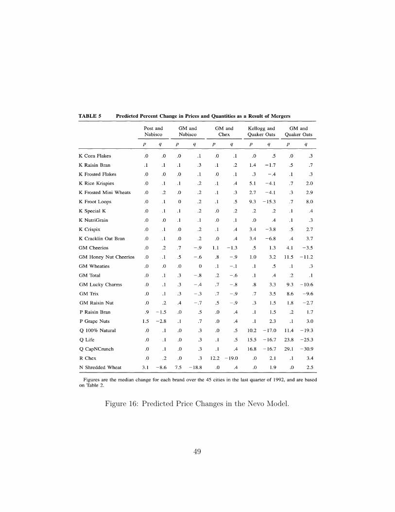
412 / THE RAND JOURNAL OF ECONOMICS

TABLE 5 Predicted Percent Change in Prices and Quantities as a Result of Mergers

Post and GM and GM and Kellogg and GM and Nabisco Nabisco Chex Quaker Oats Quaker Oats

K Corn Flakes

K Raisin Bran

K Frosted Flakes

K Rice Krispies

K Frosted Mini Wheats

K Froot Loops

K Special K

K NutriGrain

K Crispix

K Cracklin Oat Bran

GM Cheerios

GM Honey Nut Cheerios

GM Wheaties

GM Total

GM Lucky Charms

GM Trix

GM Raisin Nut

P Raisin Bran

P Grape Nuts

Q 100% Natural

Q Life

Q CapNCrunch

R Chex

N Shredded Wheat

Figures are the median change for each brand over the 45 cities in the last quarter of 1992, and are based on Table 2.

95% confidence interval of between 4.0 and 13.1). A 5% cost reduction is no longer enough to offset the effects of the merger. As seen in the second column of Table 6, the cost reduction to Shredded Wheat would need to be greater than 10% (with a 95% confidence interval of between 5.1 and 21.4) in order to reach the same equilibrium outcome.

In August 1996 General Mills purchased from Ralston the Chex cereal line. This merger was examined by the federal authorities and not challenged. The increase in price is presented in the third column of Table 5.18 The predicted price increases and

The results presented here take the premerger state as prior to the Post-Nabisco merger. I also tried to simulate these mergers sequentially, i.e., take into account that Post acquired the Nabisco cereal line when computing the premerger stats. The results were essentially the same.

Figure 16: Predicted Price Changes in the Nevo Model.

49