demonstrati on of advanced biomass …€¦ · · 2016-05-02final project report . demonstrati on...

E n e r g y R e s e a r c h a n d D e v e l o p m e n t D i v i s i o n F I N A L P R O J E C T R E P O R T

DEMONSTRATION OF ADVANCED BIOMASS COMBINED HEAT AND POWER SYSTEMS IN THE AGRICULTURAL PROCESSING SECTOR

Prepared for: California Energy Commission Prepared by: West Biofuels, LLC

JUNE 2015 CE C-500-2016-035

PREPARED BY: Primary Author(s): Matthew Summers – West Biofuels Chang-hsien Liao – West Biofuels Matthew Hart – West Biofuels Robert Cattolica – UC San Diego Reinhard Seiser – UC San Diego Bryan Jenkins – UC Davis Paul Vergnani - Cha Corporation Christopher Weaver – EF & EE West Biofuels, LLC Woodland Biomass Research Center 14958 County Road 100B Woodland, CA 95776 Phone: 530-207-5996 http://www.westbiofuels.com Contract Number: PIR-11-008 Prepared for: California Energy Commission Cecelia S. Golden Contract Manager Virginia Lew Office Manager Energy Efficiency Research Office Laurie ten Hope Deputy Director ENERGY RESEARCH AND DEVELOPMENT DIVISION Robert P. Oglesby Executive Director

DISCLAIMER This report was prepared as the result of work sponsored by the California Energy Commission. It does not necessarily represent the views of the Energy Commission, its employees or the State of California. The Energy Commission, the State of California, its employees, contractors and subcontractors make no warranty, express or implied, and assume no legal liability for the information in this report; nor does any party represent that the uses of this information will not infringe upon privately owned rights. This report has not been approved or disapproved by the California Energy Commission nor has the California Energy Commission passed upon the accuracy or adequacy of the information in this report.

ACKNOWLEDGEMENTS

The authors would like to acknowledge the contributions of the following individuals and their organizations that contributed to the success of this project and the content of this report. This work could not have been completed without the hard work of these dedicated professionals:

West Biofuels – Woodland: Brandon Bruning, Andrew Ramirez, George Loveday, and Anthony Roca

West Biofuels/Headlands - San Rafael: Peter Paul, Kristen Decker, Lisa Jones. Cary Amman

University of California, San Diego: Jesse Littlefield, Dr. Ashish Bambel, Dr. Tinku Biadya, Dr. Kevin Mandich, Dr. Hui Liu, Dr. Ulrich Niemann, Prof. Richard Herz, and Prof. Kal Seshadri

Colorado State University: Dr. Dan Wise, and Dr. Dan Olsen

University of California, Davis: Kevin Copely, Patrick Fitzgerald, Michael Long, Zach McCaffrey, Brian Emmeneger, and Rob Williams

Vienna Technical University: Dr. Reinhard Rauch, Prof. Herman Hofbauer,

Güssing Renewable Energy: Reinhard Koch, Graeme Bethell, Michael Dichand, and Alexander Nunner

Consulectra, GmbH: Uwe Gayh and Dr. Stephan Weber

i

PREFACE

The California Energy Commission Energy Research and Development Division supports public interest energy research and development that will help improve the quality of life in California by bringing environmentally safe, affordable, and reliable energy services and products to the marketplace.

The Energy Research and Development Division conducts public interest research, development, and demonstration (RD&D) projects to benefit California.

The Energy Research and Development Division strives to conduct the most promising public interest energy research by partnering with RD&D entities, including individuals, businesses, utilities, and public or private research institutions.

Energy Research and Development Division funding efforts are focused on the following RD&D program areas:

• Buildings End-Use Energy Efficiency

• Energy Innovations Small Grants

• Energy-Related Environmental Research

• Energy Systems Integration

• Environmentally Preferred Advanced Generation

• Industrial/Agricultural/Water End-Use Energy Efficiency

• Renewable Energy Technologies

• Transportation

Demonstration of Advanced Biomass Combined Heat and Power Systems in the Agricultural Processing Sector is the final report for the project (contract number PIR-11-008) conducted by West Biofuels, LLC. The information from this project contributes to Energy Research and Development Division’s Industrial/Agricultural/Water End-Use Energy Efficiency Program.

For more information about the Energy Research and Development Division, please visit the Energy Commission’s website at www.energy.ca.gov/research/or contact the Energy Commission at 916-327-1551.

ii

ABSTRACT

Each year, California’s almond industry produces approximately 1,000,000 bone-dry tons of recoverable woody biomass residues such as almond shells and orchard removals and prunings. To address this under-utilized resource, the research team successfully designed and constructed a pilot-scale biomass combined heat and power system in Woodland, California that can be commercially deployed in the agricultural processing sector. The pilot-scale system is capable of processing up to six tons of biomass into 250 kilowatts of electricity and 625 kilowatts of heat for industrial use and demonstrated 65 percent cold gas efficiency. The pilot-scale facility, using a fast internally circulating fluidized bed gasifier, successfully demonstrated that a synthetic bed material could produce a catalytic tar reduction similar to that of natural sand bed material (the primary heat transfer mechanism within the gasification system) while eliminating the transfer of chromium to the ash byproduct. Catalytic tar reduction is important for high-quality gas production and the elimination of chromium allows the ash byproduct to become a valuable soil amendment. Also, the research team was able to substantially reduce emissions from the pilot-scale system by 75 to 95 percent by using activated carbon for gas filtration and selective catalytic reduction for engine emission control. Using computer modeling, they determined that commercial-scale facilities would cost less than $4,000 per kilowatt to build and would operate with 28 percent electrical efficiency and 80 percent combined heat and power efficiency. Based on the modeled parameters, a commercial-scale facility would be economically viable with a power contract of $124 per megawatt-hour with available grants and tax credits, or $165 per megawatt-hour without them. The team estimates that commercial-scale biomass combined heat and power system can reduce global warming potential by up to 70 percent when compared to California’s current electricity portfolio.

Keywords: biomass, gasification, circulating fluidized bed, agricultural residues, producer gas, syngas, tars, wood ash, lean-burn engine, selective catalytic reduction, activated carbon, NOx emissions, life-cycle analysis

Please use the following citation for this report:

Summers, Matthew; Liao, Chang-hsien; Cattolica, Robert; Seiser, Reinhard; Jenkins, Bryan; Vergnani, Paul; Weaver, Christopher; Hart, Matthew. 2015. Demonstration of Advanced Biomass Combined Heat and Power Systems in the Agricultural Processing Sector. California Energy Commission. Publication number: CEC-500-2016-035.

iii

TABLE OF CONTENTS

Acknowledgements ................................................................................................................................... i

PREFACE ................................................................................................................................................... ii

ABSTRACT .............................................................................................................................................. iii

TABLE OF CONTENTS ......................................................................................................................... iv

Introduction ........................................................................................................................................ 1

Project Purpose ................................................................................................................................... 1

Project Results ..................................................................................................................................... 2

Project Benefits ................................................................................................................................... 3

CHAPTER 1: Project Description .......................................................................................................... 5

1.1 Introduction ................................................................................................................................ 5

1.2 BCHP Technology Description ................................................................................................ 8

1.3 Project Goal ............................................................................................................................... 12

1.4 Project Objectives ..................................................................................................................... 12

CHAPTER 2: Design and Installation of the BCHP System .......................................................... 13

2.1 BCHP Process Description ...................................................................................................... 13

2.2 Operating Procedures .............................................................................................................. 17

2.3 Expected Performance Characteristics .................................................................................. 20

2.4 Fabrication and Installation of the BCHP System ............................................................... 26

CHAPTER 3: Qualification of Biomass Feedstock for BCHP Operations .................................. 37

3.1 BCHP Siting Assessment ........................................................................................................ 37

3.1.1 Biomass Tonnages Available .......................................................................................... 37

3.1.2 Geographic Location of Facilities ................................................................................... 37

3.1.3 Spatial Mapping ............................................................................................................... 38

3.1.4 Results and Analysis ........................................................................................................ 39

3.2 Biomass Thermochemical Properties .................................................................................... 41

3.2.1 Experimental Design ....................................................................................................... 41

3.2.2 Laboratory Methods ........................................................................................................ 42


3.3 Biomass Gasification Properties ............................................................................................. 46



iv


3.4 BCHP Process ........................................................................................................................... 56

3.5 Materials and Methods ............................................................................................................ 57

3.6 Results and Analysis ................................................................................................................ 66

CHAPTER 4: Emission Control Systems Performance ................................................................... 73

4.1 Flue Gas Adsorber System with Microwave Regeneration ............................................... 73

4.1.1 Background ....................................................................................................................... 73

4.1.2 Materials and Methods .................................................................................................... 74


4.2 Compact Selective Catalytic Reduction System .................................................................. 82

4.2.1 Background ....................................................................................................................... 82

4.2.2 Materials and Methods .................................................................................................... 84


4.2.4 Meeting California Emission Limits .............................................................................. 93

CHAPTER 5: Synthetic Bed Material and Ash Recovery ............................................................... 95

5.1 Flow Reactor Study of Synthetic Bed Material .................................................................... 95




5.1.4 Catalyst Characterizations ............................................................................................ 104

5.1.5 Conclusions ..................................................................................................................... 108

5.2 Fixed Bed Reactor Study of Synthetic Bed Material .......................................................... 109

5.2.1 Experimental Design ..................................................................................................... 109

5.2.2 Laboratory Methods ...................................................................................................... 111

5.2.3 Results and Analysis ...................................................................................................... 113

5.3 Laboratory Gasifier Reactor Study of Synthetic Bed Material ......................................... 118

5.3.1 Experimental Design ..................................................................................................... 118

5.3.2 Laboratory Methods ...................................................................................................... 119

5.3.3 Results and Analysis ...................................................................................................... 120

CHAPTER 6 Technical and Economic Analysis for BCHP Commercialization ................. 123

6.1 BCHP Process Model ............................................................................................................. 123

6.1.1 Model Basis ..................................................................................................................... 123

v

6.1.2 Model Description.......................................................................................................... 125

6.1.3 Model Performance ........................................................................................................ 128

6.1.4 Evaluation of Commercial Scale BCHP Systems ....................................................... 129

6.1.5 Advanced System Modeling ........................................................................................ 131

6.1.6 Results .............................................................................................................................. 135

6.1.7 Analysis of Model .......................................................................................................... 141

6.8 BCHP Life Cycle Model ........................................................................................................ 142



6.9 BCHP Economic Model ......................................................................................................... 144

6.9.1 Model Basis ..................................................................................................................... 144


6.9.3 Economic Analysis ......................................................................................................... 148

6.9.4 No Incentives Scenario: ................................................................................................. 149


6.9.6 Conclusions: .................................................................................................................... 158

6.9.7 Evaluation of Commercial Scale BCHP Systems ....................................................... 158

CHAPTER 7: Production Readiness of the BCHP System ........................................................... 161

7.1 Production Requirements ..................................................................................................... 162

7.1.1. Manufacturing Facilities ............................................................................................... 166

7.1.2 Investment Requirements ............................................................................................. 166

7.1.3 Implementation Plan ..................................................................................................... 168

7.2 Conclusions ............................................................................................................................. 170

7.2.1 Technical Feasibility of BCHP ...................................................................................... 170

7.2.2 Environmental Feasibility of BCHP ............................................................................ 171

7.2.3 Economic Feasibility of BCHP...................................................................................... 171

7.3 Project Benefits ....................................................................................................................... 172

7.4 Recommendations .................................................................................................................. 172

Glossary .................................................................................................................................................. 173

REFERENCES ........................................................................................................................................ 177

APPENDIX A: BCHP Installation Plan and Details of BCHP Plant Design ............................... A

BCHP INSTALLATION PLAN ........................................................................................................ A-1

vi

APPENDIX B: BCHP System Test Plan and Details of BCHP Plant Performance ...................... B

BCHP System Test Plan..................................................................................................................... B-1

APPENDIX C: Technology Transfer Plan and Activities ................................................................ C

Technology Transfer Plan ................................................................................................................. C-1

Conference Presentations .................................................................................................................. C-2

LIST OF FIGURES

Figure 1.1: Biomass Resources in California from Various Sectors Including Technical Potential and Gross Resources .................................................................................................................................. 6

Figure 1.2: Steps in the Biomass Combined Heat and Power System Using a Gasifier ................... 9

Figure 1.3: Schematic of (a) Güssing FICFB Gasifier and (b) West Biofuels’ DFB Gasifier ........... 10

Figure 1.4. Gasifier and Engine Availability History for Güssing BCHP Operations 2002-2011 . 10

Figure 2.1: Dual Fluidized Bed Gasification System at Woodland Biomass Research Center Prior to the Installation of FICFB ..................................................................................................................... 13

Figure 2.2: Biomass Combined Heat and Power Plant in Güssing, Austria .................................... 14

Figure 2.3: Güssing BCHP Plant Layout ............................................................................................... 14

Figure 2.4: Process Flow Diagram for Woodland BCHP Plant ......................................................... 16

Figure 2.5: Woodland BCHP Plant Design Represented with 3D CAD Model .............................. 17

Figure 2.6: Woodland BCHP Plant Mass and Energy Flow Diagram – Gasifier Side .................... 21

Figure 2.7: Woodland BCHP Plant Mass and Energy Flow Diagram – Combustor Side .............. 22

Figure 2.8: Biomass Feeder System ........................................................................................................ 28

Figure 2.9: Gasifier System ..................................................................................................................... 29

Figure 2.10: Combustor System ............................................................................................................. 29

Figure 2.11: Cyclone and Loop Seal System ......................................................................................... 30

Figure 2.12: Gas Cooler and Heat Recovery System ........................................................................... 31

Figure 2.13: Steam Generation System .................................................................................................. 32

Figure 2.14: Product Gas Filter System ................................................................................................. 33

Figure 2.15: Product Gas Scrubber System ........................................................................................... 34

Figure 2.16: Flue Gas Filter and Exhaust System ................................................................................. 35

Figure 2.17: Engine and Flare System ................................................................................................... 36

vii

Figure 3.1: Location of Proxy Locations for BCHP Facilities ............................................................. 38

Figure 3.2: Location of Almond Orchards in California ..................................................................... 39

Figure 3.3: Locations for Potential Development of BCHP Technology .......................................... 40

Figure 3.4: Removal of Crucibles From Furnace During Determination of Volatiles .................... 43

Figure 3.5: Solvent Recirculation Isokinetic Tar Sampling Nozzle ................................................... 48

Figure 3.6: X-ray Diffraction Patterns Determined on Finely-Powdered Ashes using Cu Kα Radiation ................................................................................................................................................... 49

Figure 3.7: X-ray Diffraction Patterns of Bed Materials ...................................................................... 50

Figure 3.8: SEM BSE Image of Used Bed Material .............................................................................. 51

Figure 3.9: Higher-Resolution SEM BSE Image of Bed Material ....................................................... 52

Figure 3.10: SEM BSE Image of Bed Material for Detailed Analysis ................................................ 53

Figure 3.11: X-ray Kα Density Maps ..................................................................................................... 54

Figure 3.12: Pictures of Sampling Nozzle ............................................................................................. 55

Figure 4.1: Motor Drive Systems (left) and SCADA Operator Interface (right) in BCHP Control Room .......................................................................................................................................................... 57

Figure 4.2: Various Sensor Systems Utilized to Monitor and Control the BCHP Process ............. 57

Figure 4.3: SCADA System Architecture Based on PLC Input/Output Modules Connected to Operator Computer System .................................................................................................................... 58

Figure 4.4: SCADA System PLC Panels on the BCHP Plant .............................................................. 59

Figure 4.5: SCADA System Front Panel ................................................................................................ 59

Figure 4.6: Locations of Sensors on FICFB Reactors ........................................................................... 62

Figure 4.7: Locations of Sensors on Heat Recovery System ............................................................... 63

Figure 4.8: Locations of Sensors on Steam Generator System ........................................................... 63

Figure 4.9: Locations of Sensors on Product Gas Filter System ......................................................... 64

Figure 4.10: Locations of Sensors on Product Gas Scrubber System ................................................ 64

Figure 4.11: Location of Sensors on Product Gas Handling System ................................................. 65

Figure 4.12: Locations of Sensors on Flue Gas Handling System...................................................... 65

Figure 4.13: Gasifier Bed Temperature During Plant Start-Up ......................................................... 66

Figure 4.14: Differential Pressure Across the Gasifier Bed during Start-Up ................................... 67

viii

Figure 4.15: External Fuel Metering During Plant Start-Up .............................................................. 68

Figure 4.16: Operating Conditions From Woodland FICFB (top) and Güssing FICFB (bottom) . 70

Figure 5.1: Adsorption Process Flow Diagram .................................................................................... 74

Figure 5.2: Exhaust Gas Heat Exchanger .............................................................................................. 75

Figure 5.3: Carbon Adsorber .................................................................................................................. 76

Figure 5.4: Microwave Regeneration Process Flow Diagram ............................................................ 77

Figure 5.5: Trailer-Mounted Carbon Regeneration Unit .................................................................... 78

Figure 5.6: Microwave Destruction Reactor Skid ................................................................................ 79

Figure 5.7: Contaminant Concentration from Gasifier Run 3/9/15 ................................................... 81

Figure 5.8: Test-Engine Emissions as a Function of Air-fuel Equivalence Ratio, Lambda ............ 83

Figure 5.9: Schematic of Engine Control System ................................................................................. 85

Figure 5.10: Performance of Engine Control System .......................................................................... 87

Figure 5.11: Diagram of the Developmental Exhaust Emission Control System ............................ 88

Figure 5.12: Photograph of the Developmental Exhaust Emission Control System ...................... 89

Figure 5.13: Diagram of the Final Exhaust Emission Control System .............................................. 90

Figure 6.1: Schematic Representation of the Steam Reforming Unit with a Fixed-Bed Reactor ... 96

Figure 6.2: Tar Removal Efficiency in Ni vs. Ni-Fe (a) and Ni-Fe vs. Ni-Fe-CaO (b) Catalysts .. 100

Figure 6.3: Tar Removal Activity with Variation of Temperature Over Ni-Fe-CaO Catalysts ... 101

Figure 6.4: Time-on-Stream & Regeneration Study over 1% (Ni65Fe35), 1.6% (Ni45Fe15Ca40) and 1.6% (Ni40Fe20Ca40) Catalysts for Tar Removal from Producer Gas .................................... 103

Figure 6.5: XRD Patterns of (a) 1%Ca, (b) 1.6%(Ni60Ca40), (c) 1.6%(Ni45Fe15Ca40), (d) 1.6%(Ni35Fe25Ca40), (e) 1.6%(Ni20Fe40Ca40), (f) 1%(Fe60Ca40) and (g) Spent Catalyst of 1.6%(Ni40Fe20Ca40) .............................................................................................................................. 105

Figure 6.6: TPR Profiles of (a) Carbo HSP, (b) 1.6%(Ni60Ca40), (c) 1.6%(Ni45Fe15Ca40), (d) 1.6%(Ni35Fe25Ca40), (e) 1.6%(Ni20Fe40Ca40), (f) 1%(Fe60Ca40) and (g) 1%(Ni50Fe50) ........... 106

Figure 6.7: SEM Images of Freshly Reduced and Spent Catalysts of 1.6% (Ni45Fe15Ca40) (a,b), 1.6% (Ni40Fe20Ca40) (c,d) and 1% (Ni65Fe35) (e,f), Respectively .................................................. 107

Figure 6.8: TEM Images of Freshly Reduced (a, d) and Spent Catalysts of 1.6%(Ni40Fe20Ca40) (b, c) and 1%(Ni65Fe35) (e, f) Respectively ........................................................................................ 108

Figure 6.9: Schematic of Portable Tar Reformer ................................................................................ 110

ix

Figure 6.10: Photograph of Fixed-Bed Tar Reformer ........................................................................ 111

Figure 6.11: Catalyst in Reactor Tube (a) and After Removal (b) .................................................... 114

Figure 6.12: Deactivation of Nickel Catalyst Depending on Tar Type ........................................... 115

Figure 6.13: Deactivation of Nickel Catalyst Depending on Catalyst Loading ............................. 115

Figure 6.14: Deactivation of Nickel Catalyst Depending on Temperature .................................... 116

Figure 6.15: Operation of Tar Reformer on Producer Gas ............................................................... 117

Figure 6.16: Schematic of the Fluidized Bed Gasifier ........................................................................ 120

Figure 6.17: Bed Pressure of the CarboHSP Material (left), and 20-pt Average of the Bed Pressure (right) ....................................................................................................................................... 121

Figure 6.18: Bed pressure of the NARCO Investocast 60 bed material (left), and 20-pt average of the bed pressure (right) ......................................................................................................................... 121

Figure 7.1: Screenshot of the Flow Diagram in Aspen’s User Interface ......................................... 123

Figure 7.2: Rendering of the Reactor with Streams Labeled Similar to the Aspen Flowsheet .... 124

Figure 7.3: Process Boundaries for the Gasifier Vessel ..................................................................... 125

Figure 7.4: (a) Dual Fluidized-Bed System and (b) Model Setup .................................................... 133

Figure 7.5: Locations of Temperature Sensors ................................................................................... 134

Figure 7.6: Particle Circulation in the Dual Fluidized-Bed System ................................................. 136

Figure 7.7: Section View of Solid Volume Fractions ......................................................................... 136

Figure 7.8: CO (Top), H2O (Middle), and H2 (Bottom) Distributions ............................................ 138

Figure 7.9: (a) O2 Gas Concentration Distribution and (B) Temperature Distribution................ 139

Figure 7.10: Producer Gas Composition Comparison (Dry Basis) .................................................. 140

Figure 7.11: Gasifier Temperature Comparison ................................................................................ 140

Figure 7.12: Combustor Temperature Comparison .......................................................................... 141

Figure 7.13: New Market Tax Credit Financial Structure ................................................................. 146

Figure 8.1: Cover Page and Contents of a Typical Bid Lot for a BCHP Plant ............................... 165

Figure 8.2 Physical Plant Costs for BCHP Project as a Function of Project Size in Mwe ............. 167

Figure 8.3: Physical Plant Costs For BCHP Project as a Function of Project Size in $/Mwe ........ 168

Figure 8.4: Project Development Process Phases For A BCHP Project ........................................... 169

Figure 8.5: Potential Implementation Schedule for a BCHP Project ............................................... 170

x

LIST OF TABLES

Table 1.1: Natural Gas and Power Requirements for the Almond Agricultural Sector in California. .................................................................................................................................................... 7

Table 1.2: Current Utilization and Potential Net Power, Natural Gas Replacement, and Economic Value. ......................................................................................................................................... 8

Table 1.3: Producer Gas Properties from West Biofuels’ Dual Fluidized Bed Gasifier and From the Güssing FICFB Gasifier..................................................................................................................... 11

Table 2.1: Syngas Composition for FICFB ............................................................................................ 15

Table 2.2: Gasifier Stream Characteristics of the Woodland BCHP Plant Design .......................... 23

Table 2.3: Engineering Bid Packages for the Woodland BCHP Plant ............................................... 27

Table 3.1: Almond Biomass Resource Estimate ................................................................................... 37

Table 3.2: Overview of Thermochemical Properties ........................................................................... 41

Table 3.3: Overview of Experimental Tests .......................................................................................... 42

Table 3.4: Standard Methods and Analytical Procedures .................................................................. 44

Table 3.5: Results of Thermochemical Properties ................................................................................ 45

Table 3.6: Results of Feedstock Mineral Analysis ................................................................................ 46

Table 3.7: Composition of Bed and Rims .............................................................................................. 54

Table 3.8: Gravimetric Tar Analysis Results ........................................................................................ 55

Table 4.1: Sensors Used in SCADA System to Monitor the BCHP Operation and Performance . 60

Table 4.2: External Fuel Consumption for Start-Up of BCHP Plant ................................................. 68

Table 4.3: Operating Conditions for Agricultural Biomass Test Runs in Woodland BCHP ......... 69

Table 4.4: Product Gas Composition From Woodland FICFB in Comparison With Güssing FICFB ......................................................................................................................................................... 71

Table 4.5: Energy Flows of Process Units During Gas Production Runs of Woodland BCHP ..... 72

Table 5.1: Summary of Adsorber Contaminant Removal .................................................................. 81

Table 5.2: Summary of Weights From Regeneration .......................................................................... 82

Table 5.3: Engine Configuration ............................................................................................................ 85

Table 5.4: Engine Operation on a Propane/Nitrogen Mixture ........................................................... 86

Table 5.5: Engine Operation on Producer Gas at Low Load .............................................................. 92

xi

Table 5.6: Engine Operation on Producer Gas at Intermediate Load ............................................... 93

Table 5.7: Projected Emissions for Gasification Plant ......................................................................... 94

Table 6.1: Calculated Ni-, Fe-, and CaO-based Composite Catalyst Loading on Carbo HSP ....... 98

Table 6.2: C7H8, C2H4, and CH4 Conversion Efficiency, H2 Conc., COx Selectivity, and H2/CO Ratio over Ni-Fe-CaO/Carbo Catalysts (750°C) ................................................................................. 102

Table 6.3: Overview of Target Test Composition .............................................................................. 112

Table 6.4: Tar Reformer Outlet Composition ..................................................................................... 118

Table 6.5: Composition and properties of Investocast 60 and CarboHSP bed materials. Source: NARCO, Carbo Ceramics, and Chase (1998). .................................................................................... 119

Table 6.6: Heat Capacities of Bed Material Components ................................................................. 119

Table 6.7: Bed Pressures for Investocast and Carbohsp Bed Materials .......................................... 122

Table 7.1: Components Defined in Simulation .................................................................................. 126

Table 7.2: Material Input to the Reactor .............................................................................................. 127

Table 7.3: Process Flow Rates for the Model ...................................................................................... 127

Table 7.4: Bed Material Composition .................................................................................................. 128

Table 7.5: Computed Mass-Flow Rates from the Model .................................................................. 128

Table 7.6: Gas Composition in Mole Fractions .................................................................................. 129

Table 7.7: Process Flow Rates for the Model ...................................................................................... 130

Table 7.8: Computed Mass-Flow Rates from the Model .................................................................. 130

Table 7.9: Gas Composition in Mole Fractions .................................................................................. 130

Table 7.10: Biomass Gasification and Combution Heterogeneous and Homogenous Reactions. .................................................................................................................................................................. 132

Table 7.11: Biomass Properties ............................................................................................................. 135

Table 7.12: Model Settings .................................................................................................................... 135

Table 7.13: California Grid Mix ............................................................................................................ 143

Table 7.14: Summary of Greenhouse Gases and Criteria Air Pollutant Emissions for Almond Biomass BCHP ........................................................................................................................................ 144

Table 7.15: Base Case Economic Assumptions ................................................................................... 148

Table 7.16: Comparison of the LCOE for BCHP Production with Various Credit and Investment Scenarios .................................................................................................................................................. 149

xii

Table 7.17: Comparison of LCOE from Black and Veatch Model to Base Case Model ................ 151

Table 7.18: Sensitivity Analysis of Capital Cost – LCOE Summary ............................................... 152

Table 7.19: Sensitivity Analysis of Heat Price – LCOE Summary ................................................... 153

Table 7.20: Sensitivity Analysis of Fuel Costs – LCOE Summary ................................................... 154

Table 7.21: Sensitivity Analysis of Interest Rate – LCOE Summary ............................................... 155

Table 7.22: Sensitivity Analysis of Return on Investment – LCOE Summary ............................... 156

Table 7.23: WACC on ROE and Debt Interest Rate (80% Financing) ............................................. 157

Table 7.24: Sensitivity Analysis of WACC – LCOE Summary......................................................... 157

Table 7.25: Schedule of Potential SB 1122 Contract Acceptance Prices .......................................... 159

Table 7.26: Projected NPV for the Four BCHP Financing Scenarios and SB 1122 Contract Price .................................................................................................................................................................. 160

Table 8.1: BCHP Projects Based on the FICFB Gasifier Technology Developed Worldwide ...... 161

Table 8.2: Projected Physical Plant Costs for Components of 3mwe BCHP Project ..................... 167

xiii

EXECUTIVE SUMMARY

Introduction California adopted the Renewable Portfolio Standard requiring the state’s utilities to procure 33 percent of their electricity demands from eligible renewable resources by 2020. This goal will require developing and installing renewable power systems including solar, wind and biomass. Solar and wind energy resources are currently widely deployed in California and supported by a variety of incentive programs. Biomass resources, however, have not been developed to a similar extent because of economic and technological issues related to costs and environmental compliance.

This project demonstrates a robust, efficient, community-scale and environmentally sound Biomass Combined Heat and Power (BCHP) system in Woodland, California that can be commercially used in California’s agricultural processing sector. There is a massive potential to deploy BCHP facilities in California that has not been realized due to barriers this project addresses:

• Technological: While biomass gasifiers and combustors have been around for many years, there have been insufficient demonstrations of reliable, integrated BCHP systems.

• Market: Consumer knowledge about BCHP has been limited due to lack of demonstrated market viable systems. In addition, the major incentive programs of the utilities like Self-Generation Incentive Program have not considered BCHP for incentives.

• Institutional and Environmental: Ability to achieve very restrictive emissions control standards in the California air districts is required for deployment of the BCHP technology. In addition, any residues from the BCHP process have to be able to be recycled to the land and not become a disposal issue.

Project Purpose The project fulfilled the following objectives to demonstrate that BCHP can be a commercially viable source of renewable energy for the agricultural processing sector:

• Qualify the use of processing biomass feedstock for BCHP operations.

• Demonstrate emission controls for BCHP technologies that can meet California Air Resources Board and Regional Air District Standards.

• Demonstrate an ash byproduct suitable for recycling as fertilizer back to agriculture.

• Demonstrate electrical efficiency and heat recovery guidelines for BCHP that can be used by the California utilities to develop incentive and interconnection programs for BCHP technologies in the agricultural and food processing sector.

• Develop a techno/economic model for commercialization of BCHP to include a carbon and material life cycle analysis.

1

Project Results The project designed, constructed, and operated a commercial pilot of the BCHP and tested its performance with agricultural biomass. This pilot testing, and a host of supporting laboratory and modeling activities, established the following project results:

• The total sustainable resource of agricultural biomass from the almond production sector is 1,002,360 tons per year. This resource is distributed through 22 California counties and can result in a total power production of 165 megawatts (MWe) of electrical energy and 85 megawatts of thermal energy (MWth) from small-scale BCHP facilities.

• The emissions from BCHP plants can be controlled such that air quality standards can be met by using a combination of extended-lean burn combustion of product gas, oxidation catalyst, and selective catalytic reduction (SCR) emissions controls. The project demonstrated 74-92% oxides of nitrogen (NOx) emissions reductions and achieved single digit parts per million (ppm) levels needed to meet the most stringent standards. The carbon monoxide (CO) emissions were reduced to below 400 ppm using the system but an optimized oxidation catalyst was needed to achieve lower levels required in certain air districts.

• The use of synthetic bed material in a BCHP is feasible and can produce catalytic tar-reduction results similar to natural olivine bed material used in Europe. This inert bed material reduces any risk of transfer of chromium to ash via bed-material attrition and eliminates the contamination of ash with chromium. Ash composition is dictated by the composition of the agricultural biomass feedstock which was shown to be compatible with standards for recycling to land.

• The cold gas efficiency of the pilot BCHP system was 65% when including supplemental fuel and 81% with supplemental fuel eliminated in a commercial sized system. This demonstrates that an overall electrical efficiency of 28.4% and a CHP efficiency greater than 80% are achievable using a lean-burn engine generator in a commercial system.

• The production of commercial BCHP facilities for a cost of less than $4,000 per kilowatt of electricity produced (kWe) was shown to be feasible and production ready. Commercial projects using BCHP technology with a power contract of $124 per megawatt hour (MWh) were shown to be economically feasible assuming 20% return on investment for projects that can successfully utilize grant funding and available tax credits. Price increases in the California Senate Bill 1122 (2012, Rubio, Ch. 612) price mechanism would be required for projects that cannot take full advantage of these grant and tax opportunities.

• The carbon dioxide (CO2) emissions of a BCHP facility were shown to be 65% lower than conventional power production on the California-grid.

2

Project Benefits The project successfully met the objectives and has demonstrated a cost-effective biomass-to- renewable energy solution for agricultural wood waste. Benefits to California investor-owned utility (IOU) ratepayers include:

• Up to 165 MWe of electrical power production valued at $188.4 million and 85 MWth of thermal energy from renewable sources offsetting fossil fuel use;

• Reduced greenhouse gas emissions from transportation and disposal of agricultural wood wastes;

• Improved air quality from greatly reduced CO2, NOx and CO emissions; and

• Rural business development and investment in clean jobs.

3

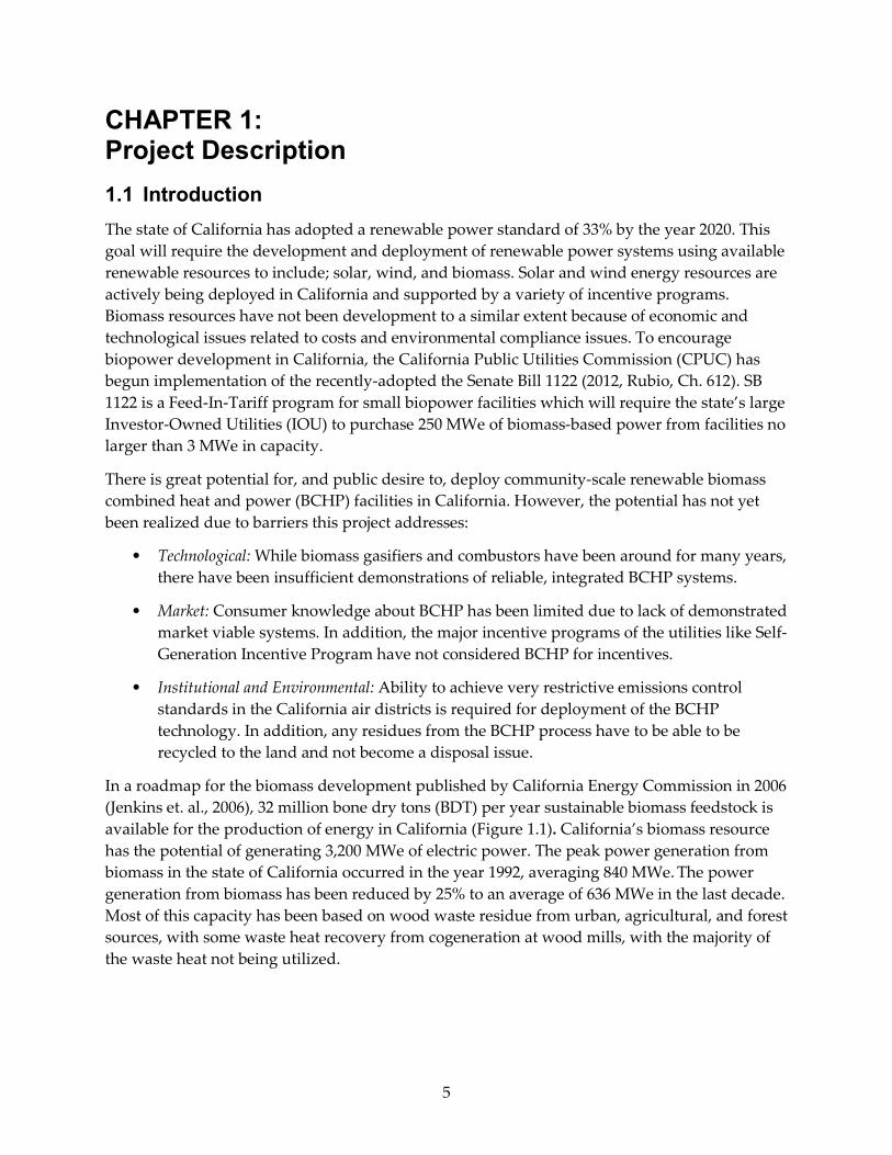
CHAPTER 1: Project Description 1.1 Introduction The state of California has adopted a renewable power standard of 33% by the year 2020. This goal will require the development and deployment of renewable power systems using available renewable resources to include; solar, wind, and biomass. Solar and wind energy resources are actively being deployed in California and supported by a variety of incentive programs. Biomass resources have not been development to a similar extent because of economic and technological issues related to costs and environmental compliance issues. To encourage biopower development in California, the California Public Utilities Commission (CPUC) has begun implementation of the recently-adopted the Senate Bill 1122 (2012, Rubio, Ch. 612). SB 1122 is a Feed-In-Tariff program for small biopower facilities which will require the state’s large Investor-Owned Utilities (IOU) to purchase 250 MWe of biomass-based power from facilities no larger than 3 MWe in capacity.

There is great potential for, and public desire to, deploy community-scale renewable biomass combined heat and power (BCHP) facilities in California. However, the potential has not yet been realized due to barriers this project addresses:

• Technological: While biomass gasifiers and combustors have been around for many years, there have been insufficient demonstrations of reliable, integrated BCHP systems.

• Market: Consumer knowledge about BCHP has been limited due to lack of demonstrated market viable systems. In addition, the major incentive programs of the utilities like Self-Generation Incentive Program have not considered BCHP for incentives.

• Institutional and Environmental: Ability to achieve very restrictive emissions control standards in the California air districts is required for deployment of the BCHP technology. In addition, any residues from the BCHP process have to be able to be recycled to the land and not become a disposal issue.

In a roadmap for the biomass development published by California Energy Commission in 2006 (Jenkins et. al., 2006), 32 million bone dry tons (BDT) per year sustainable biomass feedstock is available for the production of energy in California (Figure 1.1). California’s biomass resource has the potential of generating 3,200 MWe of electric power. The peak power generation from biomass in the state of California occurred in the year 1992, averaging 840 MWe. The power generation from biomass has been reduced by 25% to an average of 636 MWe in the last decade. Most of this capacity has been based on wood waste residue from urban, agricultural, and forest sources, with some waste heat recovery from cogeneration at wood mills, with the majority of the waste heat not being utilized.

5

Figure 1.1: Biomass Resources in California from Various Sectors Including Technical Potential and Gross Resources

The proposed demonstration project broadly targets the byproduct biomass from agricultural processing for combined heat and power production. With an estimated 8 million BDT per year of sustainable byproduct biomass from agriculture processing, the proposed BCHP technology has the potential to provide as much as 800 MWe of renewable power production distributed on California grid, more than doubling the existing capacity. An additional 800 MWe would also provide up to 1,600 MWth of waste heat recovery for industrial processes. The 800 MWe of renewable power from California’s agricultural biomass is equivalent to replacing 125 billion cubic feet (ft3) of natural gas and carbon dioxide (CO2) emissions of 7.9 million tons per year. If waste heat recovery is incorporated as a replacement for natural gas utilization the savings in natural gas and CO2 emission savings triples.

The almond agricultural sector is chosen as the primary base case for this demonstration project since it has sufficient biomass resources to become self-sustaining in energy as a sector and thus has an economic incentive to implement the proposed technology. The California almond industry has an under-utilized biomass resource that has the potential of benefiting the IOU ratepayers in California by providing 165 MWe of distributed power supplying the entire estimated power requirement for almond production and processing (85 MWe), and reducing natural gas utilization by 24 billion ft3 and CO2 emissions by 1.5 million tons annually. With waste heat recovery using the proposed BCHP technology natural gas replacement and CO2 emission savings triples. The energy efficiency of the proposed BCHP technology has been demonstrated at the Güssing Renewable Energy power production facility in Güssing, Austria for the past ten years (Weber et. al., 2013). Reliable power production at 25% efficiency and waste heat recovery (primarily for district heating) above 55% has been demonstrated for an overall efficiency greater than 80%. This high energy-efficiency and reliability, combined with

6

environmental compliance technologies provided by West Biofuels and collaborators, provides a high-quality power production system that can be demonstrated to be both economically and environmental successful in California. The dual fluidized bed (DFB) gasification process produces a high-quality synthetic gas (syngas) with a high heating value that can be used in internal combustion (IC) engines and can be operated to minimize emissions. In addition, the syngas that is produced has been reformed into synthetic natural gas (98% methane) at demonstration scale and has been used to produce synthetic Fischer-Tropsch diesel fuel at the laboratory scale at the Güssing facility. The proposed demonstration project which emphasizes biomass feedstock quality and environmental compliance for power and waste heat recovery also has the unique feature that it can be used in the future for testing both synthetic natural gas and synthetic liquid fuel production technologies.

California produces 876,195 acres of almonds (NASS, 2014) producing an estimated 480,000 BDT per year of shell and at least 520,000 tons per year of technically available orchard residue. The energy utilization associated with the almond production is summarized in Table 1.1.

Table 1.1: Natural Gas and Power Requirements for the Almond Agricultural Sector in California.

Energy Utilization In-field Processing Total Natural Gas (ft3/ton) 17,746 403 18,149 Electrical (kWh/ton) 896 6.7 902

Source: (Chancellor, 1981)

From this data, natural gas utilization is 14.9 billion cubic feet, and power utilizations are 744 GWh or an average of 85 MWe. This is be compared to the potential power generation from the almond biomass (shell and residues) using the BCHP technology of 156 MWe. In Table 5.2 the net power and natural gas production is presented along with the relevant economic values.

The gross income from the development of commercial BCHP plants for the almond agricultural sector (Table 1.2) would be $188.4 million in power with a cost based on an average retail price of $0.16 per kWh and a feed in tariff of $0.11 per kWh for the net production. For natural gas, the gross income using BCHP waste heat to replace natural gas purchased at $8.00 per thousand cubic feet (ft3) and the net sold for half the commercial price for other agricultural or industrial processing would be $245 million. The gross income to the almond agricultural sector could be as much as $433 million. The estimated cost of the installation of the proposed BCHP plant at the 2 to 10 MWe scale should be in the range of $5 million per MWe requiring a capital investment of $624 million for an installed capacity of 156 MWe.

7

Table 1.2: Current Utilization and Potential Net Power, Natural Gas Replacement, and Economic Value.

Current Utilization BCHP Production Net Power (GWh) 744 1366 622 Power Value -$120 M @ $0.16/kWh $68.4M @ $0.11/kWh Natural Gas (million ft3) 14.9 49 34.1

Gas Value -$119 M @ $8/1,000 ft3 $136 M @ $4/1,000 ft3

The proposed BCHP system, based on the fast internally circulation fluidized bed (FICFB) design with environmental compliance provided by West Biofuels and its collaborator, is self-sufficient in energy utilization requiring no net energy input after startup and requires no net input of water. The system generates water from the 15 to 25% water content of the biomass feedstock. The water is used to generate steam for system operation with the net production leaving the system as clean water vapor in the combustion exhaust of the gasifier. The replacement of power generated with fossil fuel by the BCHP system and the replacement of natural gas with waste recovery is substantial. The 156 MWe of power production from the almond sector biomass will replace 15.7 billion ft3 of natural gas and 0.986 million tons of CO2 per year. The waste heat utilization can replace 49 billion ft3 of natural gas and 3.08 million tons of CO2 per year.

Based on the proposed technology demonstration project, providing the economic, technical, and environmental validation for commercialization in the almond agricultural sector, it is expected that at least 5 to 10% of potential power production market could be developed with 2 to 3 plants under construction. In Europe (Austria and Germany), there are a total of 4 follow-up plants constructed based on the Güssing FICFB design with an installed capacity of 8 MWth of input wood feedstock that have been constructed over the past 5 years.

1.2 BCHP Technology Description The thermochemical conversion of biomass to energy in the form of heat and power in this project is based on a four step process: (1) Feedstock handling, (2) Reforming in a DFBG, (3) Gas Conditioning, and (4) Energy Generation. These steps are illustrated in Figure 1.2.

8

Figure 1.2: Steps in the Biomass Combined Heat and Power System Using a Gasifier

The production of syngas (primarily hydrogen [H2 ], methane [CH4], CO, and CO2) using indirect heating of the biomass in a DFB gasification process is illustrated in two configurations in Figure 1.3. Biomass is fed to a high temperature (850 degrees Centigrade [°C]) reactor containing sand-like material that is fluidized with steam to convert the volatile carbon (~70%) in the biomass into gas. The gasifier bed material is transported along with the fixed carbon (~30%) from the biomass to a second reactor where combustion raises the temperature of the bed material (950°C) and recycles it back to the gasifier. This process produces a high-quality gas with minimal nitrogen that is suitable for power production or for the synthesis of liquid fuels.

In Austria, Vienna Technical University has developed and operated a DFB design (shown in Figure 1.3a) at commercial demonstration scale (65 tons/day, 2 MWe) using a FICFB gasifier operating on forest wood over the past 10 years with high reliability and safety, with as much as 7,000 hours per year power production (80% availability) as shown in Figure 1.4. The system produces 2 MWe from a biomass thermal input of 8 MWth for an electrical efficiency of 25%. With the inclusion of waste heat recovery of 5 MWth for district heating, an overall energy efficiency of 80% is obtained with the Güssing design. The Güssing fluidized bed gasifier operates on olivine bed material, a naturally occurring mineral composed of magnesium (Mg), iron (Fe), and silicon dioxide (SiO2). Olivine in natural formations includes trace amounts of chromium. Through attrition, chromium will appear in the ash eliminating the possibility of recycling the ash.

9

Figure 1.3: Schematic of (a) Güssing FICFB Gasifier and (b) West Biofuels’ DFB Gasifier

(a) (b)

For application to California agricultural biomass, this is a significant environmental issue. The potential fertilizer would also bring in additional revenue if it were sold. The FICFB system is being deployed in Europe at a 2-3 MWe scale with wood feedstock. This technology, however, cannot be deployed for either wood or agricultural biomass in California because of more restrictive emission standards than in Europe and the necessity of disposal of the ash from the gasification process which cannot be recycled back to agriculture.

Figure 1.4. Gasifier and Engine Availability History for Güssing BCHP Operations 2002-2011

10

West Biofuels, a California Corporation, in collaboration with the University of California (UC) (San Diego, Davis, and Berkeley) has developed a BCHP system using a DFB gasifier (5 ton/day, wood feedstock, 140 kWe power) at an industrial-agriculture research facility in Woodland, California, within the service area of the Pacific Gas & Electric Company. This facility has been operated over the last two years to evaluate gasification of biomass feedstock, develop gasifier bed materials, and develop emission controls for power production to meet California Air Resources Board (CARB) standards. A schematic of the West Biofuels DFB gasifier is presented in Figure 1.3(b).

A comparison of the measured gas composition produced from the two DFB gasifier designs is presented in Table 1.3. The Güssing design produces gas with a 20% higher heating value with higher H2 and lower CO and also has lower tars than the West Biofuels design. However, using three-way-catalyst emission control, the West Biofuels system has much lower engine emissions of NOx and CO than the Güssing system. The Güssing system has an oxidation catalyst producing a 90% reduction of CO (300 ppm) and no control of the NOx (354 ppm) both far in excess of CARB standards.

Table 1.3: Producer Gas Properties from West Biofuels’ Dual Fluidized Bed Gasifier and From the Güssing FICFB Gasifier.

Gas Composition West Biofuels DFB Gasifier

Güssing Renewable Energy – FICFB Gasifier

H2 21.6% 35% - 45% CH4 9.9 % 9% - 11% CO 30.2 % 19% - 23% CO2 26.0 % 20% - 25% N2 10.2% < 2% Tars (mg/m3) 2000 25 H2/CO Ratio 0.72 1.8 HHV (MJ/Nm3) 10.5 12.1 NOX (ppm) 7.3 (three-way catalyst) 354 (no control) CO (ppm) 7.7 (three-way catalyst) 300 (with oxidation catalyst)

West Biofuels has demonstrated the production of clean ash using an inert bed material, based on an engineered ceramic 300-400 micron particle, which can be used to replace the olivine bed material in the Güssing gasification process shown in Figure 1.3a. In addition, West Biofuels, in collaboration with the University of California, has demonstrated as indicated in Table 1.3, superior emissions control that can meet CARB standards using the DFB design in Figure 1.3b.

The proposed BCHP project combines technologies developed by West Biofuels (bed material producing clean ash and emission controls) and Güssing Renewable Energy America (superior gas quality, reliability, and safety) to provide BCHP operational performance, environmental compliance, and techno/economic analysis with the goal of demonstrating a robust, efficient, and an environmentally sound BCHP system that can be commercially deployed in the agricultural processing sector in California.

11

1.3 Project Goal The goal of this project is to demonstrate a robust, efficient, and environmentally sound BCHP system that can be commercially deployed in the agricultural processing sector in California.

1.4 Project Objectives In order to address the above goal of demonstrating BCHP in California, the following objectives and numerical targets were developed for the project:

• Qualify the use of almond biomass feedstock for BCHP operations (Target: Establish that the amount of 1.5 million tons of available almond biomass is feasible for gasification including shells, tree removal, and pruning wood)

• Demonstrate emission controls for BCHP technologies that can meet CARB and Regional Air District Standards (Targets: NOx emissions below 0.07 lbs/MWh; CO emissions below 0.10 lbs/MWh; volatile organic compounds (VOC) emissions below 0.02 lbs/MWh).

• Demonstrate an ash byproduct suitable for recycling as fertilizer back to agriculture (Targets: chromium composition in ash byproduct is less than 500 milligrams per kilogram (mg/kg); composition of other compounds below California non-hazardous ash standards)

• Demonstrate electrical efficiency and heat recovery guidelines for BCHP that can be used by the California utilities to develop incentive and interconnection programs for BCHP technologies in the agricultural and food processing sector (Targets: Overall electrical efficiency of 22%; combined heat and power efficiency of 65%)

Develop a techno/economic model for commercialization of BCHP to include a carbon and material life cycle analysis (Targets: Installed cost for commercial system less than $4,000 per kWe; Minimum acceptable rate of return of 12% for potential commercial projects; Carbon emissions that are 70% less than conventional power and heating at an agricultural processing facility).

12

CHAPTER 2: Design and Installation of the BCHP System The first activity for this project was to design and install the gasification technology so that the performance testing on agricultural feedstock could take place. The West Biofuels facility had an existing DFB gasifier system (Figure 2.1) that was extensively modified with the FICFB gasifier to complete a 250 kWe BCHP system on-site. The gasifier system was designed by the project team, with the support of collaborators in Europe (Austria and Germany), to be fabricated and installed at the Woodland Biomass Research Center.

Figure 2.1: Dual Fluidized Bed Gasification System at Woodland Biomass Research Center Prior to the Installation of FICFB

2.1 BCHP Process Description The BCHP system designed for the Woodland Biomass Research Center is an FICFB gasification system with 1 MWth or a biomass feed-rate of up to 6 tons per day in order to generate gas for up to 250 kW of electrical production with an (IC) engine generator. The FICFB gasification system is the minimum scale necessary to model the thermochemical conversion of biomass in a FICFB gasifier using refractory insulation and employing real-world operating conditions. The West Biofuels pilot FICFB system is designed based on the original commercial FICFB plant in Güssing, Austria (Figure 2.2). The Güssing plant (8 MWth, 2 MWe, 50 ton per day) is 8 times the scale of the plant designed for Woodland.

13

Figure 2.2: Biomass Combined Heat and Power Plant in Güssing, Austria

The West Biofuels pilot FICFB was designed to improve upon the original design using data collected from 12-years of commercial operations in Europe and the experience and knowledge of the operators. The project team spent several weeks and multiple trips to Austria to refine a design that captured the best available knowledge about the technology and improved several of the problem areas that were identified.

Figure 2.3: Güssing BCHP Plant Layout

14

The layout of the Güssing BCHP plant was largely imitated for the Woodland plant. The Güssing plant layout is shown in Figure 2.3 and shows the major components of the process including reactors, gas handling, and gas utilization. The main difference in Woodland is that the gas that does not go to the engine is sent to a flare instead of a boiler unit, but all other process units are similar. The boiler is required in Güssing because district heating is still required even when the engine system is being serviced so this is always a backup to the CHP system.

Table 2.1 shows the syngas composition from the commercial-scale gasifier in Güssing, Austria. The objective was to get a similar or better gas composition and quality for the Woodland BCHP facility.

Table 2.1: Syngas Composition for FICFB

Gas Composition (molar percent)

Güssing FICFB (Weber, 2013)

Hydrogen 35% - 45% Oxygen < 0.1% Nitrogen < 2% Methane 9% - 11% Carbon Monoxide 19% - 23% Carbon Dioxide 20% - 25% Ethylene 2% - 3% Ethane ~ 0.5% Ammonia (ppm) 500 - 1500

The project team developed a detailed process flow diagram for the Woodland plant (Figure 2.4) with all process flows and operating requirements specified. The team also developed a three-dimensional Computer Aided Design (CAD) model of the plant (Figure 2.5) in order to insure that the equipment would fit into the existing footprint of the facility being modified. These design activities lead to detailed design specifications for the Woodland plant that were divided into various bid packages for components of the plant.

15

Figure 2.4: Process Flow Diagram for Woodland BCHP Plant

16

Figure 2.5: Woodland BCHP Plant Design Represented with 3D CAD Model

2.2 Operating Procedures Below is a summary description of the startup, shutdown, and operation procedures for the Woodland BCHP plant. More extensive procedures are used by the plant operators and there are special procedures developed for various alarm scenarios that are not discussed here.

Normal Startup Procedure: (18-24 hours)

• Pre-fill bed material to desired level in reactor system

• Set proportional-integral-derivative (PID) constants and make current values to be default

• Bleed air out of intermediate water loop

• Fill steam generator with water

• Start water circulation, confirm pressures

• Start nitrogen and air flows to purge pressure transducers (~1 standard liter per minute [slpm])

• Start nitrogen at screw seal

• Start combustor side:

o Insure that combustor exhaust valve is open

o Start exhaust blower on combustor side

17

o Start start-up burner (first air and then propane).

o Start combustor air at third level to give additional flow.

o Start cooling water of screw

o Increase combustor start-up burner temperature in increments of 25 °C every 30 minutes to heat refractory of combustor side

o Start steam generation when temperatures rise above 105 °C in steam generator. Steam should be diverted outside until ready for bed circulation.

• At 500 °C in upper combustor with steam being produced, bed circulation can be initiated

o Biodiesel circulation must be started.

o Combination of gas recirculation and steam should be used to fluidize gasifier

o Confirm that bed circulation has been achieved with temperatures and pressure readings in the gasifier

o Continue to heat system to operating temperature of 850 °C in gasifier bed and 750 °C in gasifier freeboard

o Gas recycle can be reduced as steam increases from steam generator

• At 850 °C in gasifier and 750 °C in gasifier freeboard, biomass feeding can be initiated

o Insure that flare ignitor is on and sparking

o Slowly open valve to flare as gas recycle is reduced

o With flare valve fully open and gas recycle blower off, shut valve to gas recycle loop. Gasifier is now only fluidized with steam.

o Begin biomass feeding, at ½ rate for first five minutes

o Insure that fluidization is occurring by pressure traces and that temperatures are stable

o Once gas is detected at flare, increase to full biomass feeding rate of 5-6 tons per hour (as calibrated for feedstock)

o Once gas production is stable at flare, engine generator can be started

Normal Shutdown Procedure: (8-12 hours)

• Turn off any propane burners

• Turn off the oil heater at Switch 3 (“Burner Propane”). This will keep circulating the oil and keep the exhaust fan on).

18

• Stop feeder bin and turn off, after filling bin

• Stop bucket elevator

• Stop Komar screw and, after 10 seconds, close biomass gate valve.

• Allow for biomass and char burnout (oxygen [O2] level on combustor side should rise to 20%).

• Check that flare has stopped burning gas.

• Reduce blowers by about 10 hertz (Hz). Never decrease the gasifier flow rate without decreasing the combustor to prevent overheating of heat exchangers.

• Turn of “propane – heater” within oil heater

• Close the knife gate valve to the flare before shutting off steam to prevent air from entering. Purge gas system with extra nitrogen during the transition.

• Replace steam with nitrogen:

- Stop steam (hand valve)

- Open steam valve to outside

- Increase nitrogen flow rate into baghouse

- Increase piston compressor slightly

• Turn propane off everywhere, and last on the outside (main valve)

• Increase nitrogen into baghouse by half a turn (from 0.5 turns to 1 turns, ~1.5->~3 pounds per square inch [psi])

• Make the current values default in all control procedures once they are not called anymore by the main control program.

Normal Idling Procedure:

• If non-emergency issue needs to be addressed during operation, plant idling is the preferred method to address issue so that plant maintains operating conditions

• Stop biomass feeding and shut biomass gate valve to bin

• Reduce or stop propane burner and secondary propane if temperature needs to be reduced

• Make sure plate-heat exchanger valve is at least half-way open to insure cooling and reduce steam

• Reduce flows on combustor side by at least 10 Hz

• Close knife-gate valve to flare slightly (not all the way)

19

• Consider purging with extra nitrogen during the transition.

• Increase flow of nitrogen into baghouse

• Close knife-gate valve to flare

• Reduce combustor flow and vent steam to the outside

• Combustor set-point pressure should be -5 mbar

• Turn of “propane – heater” on oil heater

• Stop steam using hand valve)

• Open steam valve to outside

2.3 Expected Performance Characteristics The expected performance of the plant was developed using the existing performance of the FICFB systems in Austria along with the use of chemical engineering methods to balance mass and energy flows in this chemical reactor system. Table 2.2, Figure 2.6 and Figure 2.7 show the performance characteristics of the designed system using a mass and energy balance for the system. The figure shows the layout of the system process units with various streams identified flowing between these units. The specific mass and energy characteristics of the gas and solids streams are shown in the table.

20

Figure 2.6: Woodland BCHP Plant Mass and Energy Flow Diagram – Gasifier Side

21

Figure 2.7: Woodland BCHP Plant Mass and Energy Flow Diagram – Combustor Side

22

Table 2.2: Gasifier Stream Characteristics of the Woodland BCHP Plant Design

Stream G1 Temp Cp (kJ/kg.K) Stream C1 Temp Cp (kJ/kg.K)

out of gasifier 850.0 C 2.223 kj/kg.K 916.0 C 1.195 kj/kg.K

vol mass vol mass

gas flow rate 29.35 m3/min 6.26 kg/min gas flow rate 2234 m3/min 22.90 kg/min

wet vol% wet wt% wet vol% wet wt%

H2O(g) 48.00% 43.95% H2O(g) 2.92% 1.79%

H2 19.76% 2.01% Ar 0.93% 0.57%

CO 9.88% 14.07% CO 0.08% 0.07%

CO2 13.52% 30.26% CO2 7.57% 11.38%

CH4 4.84% 3.94% N2 76.93% 73.54%

C2H4 1.56% 2.22% NO 0.02% 0.02%

C2H6 0.16% 0.24% NO2 0.00% 0.00%

C3H8 0.00% 0.00% O2 11.56% 12.63%

N2 2.08% 2.96% tot 100.00% 100.00%

O2 0.21% 0.34% 513.05 Nm3/min

solid flow solid flow 14.44 g/min

Internal E (LHV)

sensible heat Internal E (LHV)

sensible heat

Energy flow 729 kW 260.5 kW Energy flow 0 kW 542.4 kW

Stream G2 temp Cp (kJ/kg.K) Stream C2 temp Cp (kJ/kg.K)

after HE 150.0 C 1.764 kj/kg.K 851.7 C 1.185 kj/kg.K

vol mass vol mass



H2O(g) 48.00% 43.95% H2O(g) 2.92% 1.79%

H2 19.76% 2.01% Ar 0.93% 0.57%

CO 9.88% 14.07% CO 0.08% 0.07%

CO2 13.52% 30.26% CO2 7.57% 11.38%

23


CH4 4.84% 3.94% N2 76.93% 73.54%

C2H4 1.56% 2.22% NO 0.02% 0.02%

C2H6 0.16% 0.24% NO2 0.00% 0.00%

C3H8 0.00% 0.00% O2 11.56% 12.63%

N2 2.08% 2.96% tot 100.00% 100.00%

O2 0.21% 0.34% 513.05 Nm3/min


Internal E (LHV)


sensible heat



after bag house

140.0 C 1.757 kj/kg.K 615.7 C 1.138 kj/kg.K

vol mass vol mass



H2O(g) 48.00% 43.95% H2O(g) 2.92% 1.79%

H2 19.76% 2.01% Ar 0.93% 0.57%

CO 9.88% 14.07% CO 0.08% 0.07%

CO2 13.52% 30.26% CO2 7.57% 11.38%

CH4 4.84% 3.94% N2 76.93% 73.54%

C2H4 1.56% 2.22% NO 0.02% 0.02%

C2H6 0.16% 0.24% NO2 0.00% 0.00%

C3H8 0.00% 0.00% O2 11.56% 12.63%

N2 2.08% 2.96% tot 100.00% 100.00%

O2 0.21% 0.34% 513.05 Nm3/min


Internal E sensible heat Internal E sensible heat

24


(LHV) (LHV)



after scrubber 40.0 C 1.554 kj/kg.K 160.0 C 1.020 kj/kg.K

vol mass vol mass



H2O(g) 7.00% 6.01% H2O(g) 2.92% 1.79%

H2 35.34% 3.37% Ar 0.93% 0.57%

CO 17.67% 23.60% CO 0.08% 0.07%

CO2 24.18% 50.75% CO2 7.57% 11.38%

CH4 8.65% 6.60% N2 76.93% 73.54%

C2H4 2.79% 3.73% NO 0.02% 0.02%

C2H6 0.28% 0.40% NO2 0.00% 0.00%

C3H8 0.00% 0.00% O2 11.56% 12.63%

N2 3.72% 4.97% tot 100.00% 100.00%

O2 0.37% 0.57% 513.05 Nm3/min


Internal E (LHV)


sensible heat

Energy flow 729 kW Energy flow 0 kW 168.5 kW

Stream S1 temp mass flow rt Stream C5 temp Cp (kJ/kg.K)

Bed Material 850.0 C 230.94 kg/min

150.0 C 1.017 kj/kg.K

Char 0.51 kg/min vol mass

LHV flow rate 254.0 kW gas flow rate 795 m3/min 22.90 kg/min

wet vol% wet wt%

25


H2O(g) 2.92% 1.79%

Ar 0.93% 0.57%

CO 0.08% 0.07%

CO2 7.57% 11.38%

N2 76.93% 73.54%

NO 0.02% 0.02%

NO2 0.00% 0.00%

O2 11.56% 12.63%

tot 100.00% 100.00%

513.05 Nm3/min

solid flow 0.00 g/min

Internal E (LHV)

sensible heat

Energy flow 0 kW 164.3 kW

2.4 Fabrication and Installation of the BCHP System In order to fabricate the Woodland BCHP plant, the fabrication of a number of custom-specified components needed to be completed. The components involved different vendor expertise from metal pressure vessel welding to high-temperature refractory molding to advanced controls. The project team took the engineering specifications and divided them into multiple bid packages (16). These bid packages were then sent to multiple vendors to determine the best fit for the requirements of the project and best overall cost. The bid packages are described in Table 2.3. The development of these bid packages has the benefit that they are a complete engineering description of the BCHP process and can be readily sent to multiple vendors to generate accurate bids for future commercial scale projects with only slight modification to account for scale. This streamlines the process of project development in a significant way.

26

Table 2.3: Engineering Bid Packages for the Woodland BCHP Plant

BID PACKAGE DESCRIPTION Product Gas Scrubber Media Structured media for the scrubber

Product Gas Scrubber Components Scrubber shell, phase separator, biodiesel pump, heat exchanger

Product Gas Filter Particulate filter for the product gas Flue Gas Particulate Filter Particulate filter for the combustor flue gas

Flue Gas Adsorber Media adsorber for removing pollutants from flue gas

Product Gas Cooler Two step heat exchanger to cool product gas from 850°C to 160°C.

Flue Gas Cooler/ Air and Steam Preheaters

Three step heat exchanger to cool flue gas from 950°C to 160°C and preheat air and steam.

Steam Generator Waste heat steam boiler for gasifier steam

Heat Recovery Fluid Loop Pressurized water system for heat recovery from gas coolers to steam generator

Main Reactor – Metal Components Metal shell, tower, and internal fluidization nozzles

Main Reactor – Refractory Lining Wear resistant and insulating refractory of reactor system

Main Reactor – Biomass Feeder & Bin

Biomass bin, feed system, and seal system for delivering biomass to gasifier reactor

Reactor Support Structure Structure that contains the main reactor and major gas handling support systems

Gasifier System Controls Complete PLC based control system for the process

Engine Generator System Skid that contains the gas engine, exhaust emissions controls, generator, electrical switchgear, and heat recovery systems

Emergency Flare An emergency flare is always needed for cases where the engine system is disabled

After sending bid packages to vendors, the bids were reviewed by the project team and the best-fit vendor was selected for fabrication of the components in the bid. Often there was an exchange between the technical team and the vendor and some specifications were modified to improve the performance, fit, or cost of the bid package. The process of fabricating all of the bid components took up-to six months to complete but onsite installation was able to proceed on some components while others were still being fabricated. Figure 2.8 through Figure 2.17 show the process flow diagrams and actual fabrications for some of the major plant components.

27

Figure 2.8: Biomass Feeder System

28

Figure 2.9: Gasifier System

Figure 2.10: Combustor System

29

Figure 2.11: Cyclone and Loop Seal System

30

Figure 2.12: Gas Cooler and Heat Recovery System

31

Figure 2.13: Steam Generation System

32

Figure 2.14: Product Gas Filter System

33

Figure 2.15: Product Gas Scrubber System

34

Figure 2.16: Flue Gas Filter and Exhaust System

35

Figure 2.17: Engine and Flare System

36

CHAPTER 3: Qualification of Biomass Feedstock for BCHP Operations Agricultural byproduct biomass is qualified as a feedstock suitable for thermochemical conversion to power and heat for agricultural processing. Almond byproduct biomass (shell, pruning, and wood) is the primary test resource. Qualifications include: determination of geographical availability, thermochemical properties, and gasification characteristics.

3.1 BCHP Siting Assessment The BCHP siting assessment can help optimize resource utilization from the geographical distribution of almond byproduct biomass in California. The Geospatial Bioenergy Systems Model (GBSM) was used to assess potential for utilizing BCHP on almond biomass resources in California. GBSM locates optimal locations for siting BCHP technology based on spatially resolved resource estimates, characterization of the technology and transportation costs. The optimal locations are determined by minimizing the cost of production through choice of technology location and allocation of resources to those technology locations. For more information on GBSM, see Parker, 2010 and Tittmann, 2010.

3.1.1 Biomass Tonnages Available Almond biomass is estimated using residue factors (BDT per acre) for almonds from the California Biomass Collaborative Resource Assessment (Williams, 2014). The estimates have been modified by adding processing residues to the orchard residues. The processing residues are based on product yield in the Energy Commission resource report (i.e.,0.6 lbs almond shells per lb almond meat). These factors were converted to per acre values by dividing statewide processing residue by the number of acres of almond crop.

Table 3.1: Almond Biomass Resource Estimate

Orchard pruning and removals

Almond shells

(BDT/ac)

Tech. Residue

(BDT) Acres

Gross Dry Basis

Conversion Factor

(BDT/ac)

Tech. Recovery

Factor

Tech. Biomass (BDT/ac)

Almonds 876,195 0.84 0.70 0.591 0.553 1,002,360

3.1.2 Geographic Location of Facilities Processors are commonly located near the orchards. The average haul distance for almonds is 26.7 kilometers (km). A set of potential locations of facilities that have been developed for high-resolution biomass facility siting in the state of California was used to determine this distance. While these facilities are not the exact locations of almond processing facilities, the combination of minimizing the hauling cost from the orchard sources of almond biomass and the high

37

resolution of the set of potential locations gives a good approximation of the best locations for these facilities and can inform the search for processing facilities in the areas around the chosen locations.

Figure 3.1: Location of Proxy Locations for BCHP Facilities

\

3.1.3 Spatial Mapping Almond biomass originates from the almond orchards found throughout the Central Valley. The locations for almond orchards were mapped at a section (roughly 1 square mile) resolution using the Pesticide Use Reporting (PUR) database. The area under almond production identified using the PUR database does not agree with the area reported by the California Department of Food and Agriculture (CDFA) at county-level resolution. CDFA values for counties were used and the values were then scaled to match section data. Biomass resource availability in each section is found by multiplying the technical residue factors in Table 3.1 with the scaled area estimates.

38

Figure 3.2: Location of Almond Orchards in California

3.1.4 Results and Analysis The analysis found 41 locations in the Central Valley (Figure 3.3) that are capable of supporting a minimum of 3 MWe of BCHP technology at each site. For locations that can support the technology, the analysis finds little difference between them in terms of cost of production (less than $0.01/kWh difference across all sites). Site specific factors not considered in this analysis, like the owner experience, local heat demands, configuration of the processing facility and

39

supplemental feedstock, will play a larger factor in the adoption of the technology than geographic resource distribution. This is to be expected with the small scale technology.

Figure 3.3: Locations for Potential Development of BCHP Technology

83% of the production potential is located in the San Joaquin Valley, which makes air quality compliance an important factor in the successful development of these projects. The remaining 17% are located in the northern parts of the Sacramento Valley and would be less constrained by air quality concerns.

40

3.2 Biomass Thermochemical Properties This section describes the testing that was conducted to determine the thermochemical properties of almond biomass types that have the potential to be used for gasification.

3.2.1 Experimental Design The experiments to determine thermochemical properties were conducted both onsite as well as at outside laboratories. Table 3.2 shows a list of thermochemical properties considered in the current project. The moisture is measured and reported on an "as received" (a.r.) basis, i.e. wet basis. Most other results are reported on a dry basis, hence the amount of drying does not affect those values. Table 3.3 summarizes the experimental tests that were conducted. The majority of analyses were performed on seven different feedstocks. Besides almond and walnut shells, woody residues from a sawmill and an urban wood collection site were analyzed.

Table 3.2: Overview of Thermochemical Properties

Property Analysis Units Relevance of Result

Moisture

Proximate analysis

wt% (a.r., as received)

High moisture increases transportation costs, lowers thermal efficiency

Ash wt% (dry) High ash content can reduce ash-melting temperature

Volatiles, fixed carbon

wt% (dry) High volatiles increase gas and tar yield

Calorific value

MJ/kg (dry, higher heating value)

Low calorific value increases transportation costs, lowers thermal efficiency

Carbon, hydrogen, nitrogen, sulfur, oxygen

Ultimate analysis wt% (dry)

High nitrogen/sulfur content can increase NH3/H2S in gas, respectively

Arsenic, mercury, selenium

Volatile metals wt% (dry)

Volatile metals may be released into product gas or exhaust gas

Ash-melting temperature

Softening point °C

Low ash-melting temperatures cause agglomeration of bed material

Ash composition

Elemental Analysis wt% (of ash) High amount of toxins may

prevent use as byproduct Source: University of California San Diego

41

Table 3.3: Overview of Experimental Tests

Alm

ond

Shel

ls

Alm

ond

Prun

ings

Alm

ond

Hul

ls

Alm

ond

Stic

ks

Wal

nut S

hells

Red

woo

d M

ill R

esid

ue

Red

woo

d B

ark

Urb

an W

ood

Was

te (F

ines

)

Urb

an W

ood

Was

te (H

ogw

ood)

Property Analysis Analyzed

Moisture

Proximate analysis

X X X X X X X X X

Ash X X X X X X X X X

Volatiles, fixed carbon X X X X X X X X X

Calorific value X X X X X X X X X

Carbon, hydrogen, nitrogen, sulfur, oxygen

Ultimate analysis X X X X X X X X X

Arsenic, mercury, selenium

Volatile metals X X

Ash-melting temperature

Softening point X X X X X X X X X

Ash composition Elemental Analysis X X X X

Source: University of California San Diego

3.2.2 Laboratory Methods Table 3.4 shows a summary of methods and procedures used for determining thermochemical properties of the fuel. Several of the tests were conducted in-house. One of them is the determination of volatile carbon by the American Society for the Testing of Materials (ASTM) Standard E872-82. In this method, the dried sample is first heated to 600°C in one furnace and then to 950°C in a second furnace. Each test is performed in triplicate in Nichrome crucibles. Figure 3.4 shows a photograph of several test crucibles as they are removed from the high-temperature furnace.

42

Figure 3.4: Removal of Crucibles From Furnace During Determination of Volatiles

Photo Credit: University of California San Diego

Other tests were conducted at outside laboratories. The ultimate analysis, calorific value, elemental and trace elements in the ash, volatile metals, and ash melting were conducted at Hazen Research Inc.

43

Table 3.4: Standard Methods and Analytical Procedures

Property Standard Method

Proximate Analysis

Moisture ASTM D3173-03, D4442-07 (2007), E871-82 (2006)

Ash ASTM D3174-04, E1755-01 (2007), E830-87 (2004)

Volatiles ASTM E872-82 (2006)

Fixed carbon By difference

Calorimetry (higher heating value at constant volume) ASTM D5865-07 (2011), E711-87

Ultimate Analysis for crude and ash samples

C, H, N, and S ASTM D5373-08 (2008) (combustion aka Dumas method), Sulfur ASTM D4239-08

O By difference

Ash fusibility ASTM D1857-04, Jenkins et al. (1996a, b) (Fuel pellet test)

Trace elements in ash ASTM D3683-04, D6357-00

Trace elements in biomass Mercury: ASTM D6414-01, Arsenic: SW846-7062, Selenium: SW846-7742

Major and minor elements in ash ASTM D2795-86, D3682-01, and D5016-08

3.2.3 Results and Analysis Table 3.5 shows the results of thermochemical properties for different feedstocks. Moisture of the samples range from 6.4% to 55% (weight %, wet basis) and is strongly influenced by time of year and storage conditions. A moisture content of up to 25% is ideal for the FICBF gasifier. The moisture is transformed to additional steam during the process serves to increase the internal steam-to-biomass ratio. This can increase hydrogen yield and lower tar concentrations. A higher moisture content will lower the gasification temperature and could lower power output and thermal efficiency. For this reason, feedstocks with more than 25% moisture (mill residue and bark) should be dried externally (with waste heat or during extended storage in dry climate). Ash content is very low (0.2%) in the Redwood mill residue. All other samples show the ash, which also includes soil or dust if present, to be between 0.9% and 8.6%. A larger amount of ash lowers the heating value of the biomass, but for operational performance in a fluidized-bed, the ash melting point is even more important than the amount of ash. This is reported further below and in section 3.3 Biomass Gasification Properties. Most of the thermochemical values are in a range for typical biomass. Almond shells and prunings show higher sulfur content than the other feedstocks. While those levels are an order of magnitude lower than that of low sulfur-coal, higher amounts of sulfur will increase the amount of hydrogen sulfide (H2S) in the product gas which in turn will form sulfur dioxide (SO2) in the exhaust. Product gas and

44

exhaust gas measurements are reported in other chapters of this report. The elemental analysis of the ash shows that the major minerals (parts per million by weight [ppmw]) in almond shells and hulls are potassium (K), aluminum (Al), and silicon (Si), while in almond prunings and sticks, they are calcum (Ca), K, and Si. When in combination, K and Si can lead to very low melting points which in turn lead to agglomeration of the bed material in a fluidized bed gasifier. Further, in a FICFB gasifier, ash may melt in the combustor and deposit along the wall of the cyclone.

Table 3.5: Results of Thermochemical Properties

Property Units Alm

ond

Shel

ls

Alm

ond

Prun

ings

Alm

ond

Hul

ls

Alm

ond

Stic

ks

Wal

nut S

hells

Red

woo

d M

ill

Res

idue

Red

woo

d B

ark

Urb

an W

ood

Was

te

(Fin

es)

Urb

an W

ood

Was

te

(Hog

woo

d)

Moisture wt% (a.r.) 6.4 9.4 12.2 9.1 8.0 32.0 55.0 10.0 13.7 Ash wt% (dry) 4.0 2.2 8.6 4.6 1.3 0.2 2.5 3.9 0.9 Volatiles wt% (dry) 74.5 76.5 71.2 75.0 77.0 80.5 68.9 77.8 79.3 Fixed carbon wt% (dry) 21.5 21.3 20.2 20.4 22.0 19.3 28.6 18.3 19.9 Calorific Value

MJ/kg (dry, HHV) 17.8 18.6 17.7 19.4 20.1 19.4 19.3 18.9 19.2

Carbon wt% (dry) 48.1 50.0 45.2 48.6 51.9 53.0 52.9 50.3 51.3 Hydrogen wt% (dry) 5.8 5.8 5.5 5.6 5.9 6.0 5.5 5.9 6.0 Nitrogen wt% (dry) 0.87 0.47 0.99 0.90 0.27 0.05 0.17 0.79 0.19 Sulfur wt% (dry) 0.027 0.029 0.020 <0.01 0.011 0.018 <0.01 Oxygen wt% (dry) 40.2 41.8 40.2 40.7 40.0 38.7 41.5 Arsenic ppmw (dry) 0.85 1.53 Mercury ppmw (dry) <0.01 0.02 Selenium ppmw (dry) <0.05 <0.05 Ash-Melting Temperature °C 9002 13181 9002 9002 7801 12021 11851 11141 10711

Description of the items marked with footnotes: 1Ash fusion determined by ASTM D1857-04. The lower "Initial Temperature" of reducing or oxidizing atmosphere is shown 2Ash fusibility determined by fuel pellet test (Jenkins et al., 1996a, b). The temperature at which light sintering is detected is shown


45

Table 3.6: Results of Feedstock Mineral Analysis

Quantity Measured Units A

lmon

d Sh

ells

Alm

ond

Prun

ings

Alm

ond

Hul

ls

Alm

ond

Stic

ks

SiO2 wt% (of ash) 8.27 9.93 9.04 8.43 Al2O3 wt% (of ash) 16.14 2.91 2.06 2.40 TiO2 wt% (of ash) 0.15 0.16 0.08 0.11 Fe2O3 wt% (of ash) 0.89 1.61 0.58 1.04 CaO wt% (of ash) 5.38 27.70 3.77 38.36 MgO wt% (of ash) 1.34 3.42 1.96 3.71 Na2O wt% (of ash) 1.72 5.78 0.93 1.07 K2O wt% (of ash) 45.90 10.40 43.79 8.41 P2O5 wt% (of ash) 3.11 6.00 2.46 2.93 SO3 wt% (of ash) 0.40 1.46 Cl wt% (of ash) 0.51 4.62 0.39 0.05 CO2 wt% (of ash) 15.49 11.19 0.00 5.32 Ba ppmw (of ash) 648 270 78 388 Cd ppmw (of ash) 4 9 <0.1 0.4 Cr ppmw (of ash) 21.7 281 14.4 44.2 Pb ppmw (of ash) <10 33 15 5 Ag ppmw (of ash) 17 36 <1 <1

Source: University of California San Diego and University of California Davis

3.3 Biomass Gasification Properties Laboratory gasification studies of almond byproduct biomass were used to determine gasification characteristics.

3.3.1 Experimental Design The overall objective of this study was to characterize the gasification of various California sourced almond biomass in the presence of different gasifying agents (air or steam). This work was performed in conjunction with the previously reported “Increasing Renewable Energy by Almond Shell Gasification” experiments (Cattolica, 2014). Gasification of thoroughly characterized almond biomass feedstock was first investigated under both air and steam conditions for a total of 16 individual experimental runs. Following the gasification runs, gasifier operating conditions, char and ash production and composition, product gas yield and composition, as well as tar production and composition were all determined through analysis of collected data and further analysis on collected samples (Cattolica, 2014). Further investigation of agglomeration potential and properties of almond biomass was then performed. Recognizing

46

the need for a more detailed understanding of biomass gasification tar production, development of a gravimetric tar protocol was introduced into the experimental plan.

3.3.1.1 Design of Agglomeration Study To further understand agglomeration relationships in almond biomass, ashed feedstock, fresh bed material, and spent bed material from air and steam gasification runs, were investigated for mineral structure and composition. Previously characterized (Cattolica, 2014) almond biomass was ashed by firing at 575°C for composite almond (S3), and separated hull (S3H) and shell (S3S) and were investigated using X-ray diffraction. Fresh and spent bed materials were investigated under both X-ray diffraction and scanning electron microscope (SEM) imaging.

3.3.1.2 Design of Gravimetric Tar Study A gravimetric tar method was implemented to better understand gasifier performance while running on almond biomass. Tars are considered to be the major contaminant in producer gas; consequently their minimization and removal is of imperative interest to thermochemical developments. However, their unstable nature, vague definition, and desire to condense dictate a complexity in accurate measurement which is only compounded by the lack of a well-developed method. The European Union (EU) Standard CEN/TS 15439 has been developed to address the issue of tar measurement and is commonly considered the default measurement method. Being such, this gravimetric method was introduced to the laboratory scale gasification experiments allowing for confirmation of the current solid phase absorption (SPA) tar sampling method. Producer gas was sampled during gasification of almond biomass in three different experiments; analysis results were then compared to expected tar concentrations for similar type gasifiers as well as SPA tar measurement results for samples taken concurrently to the gravimetric sampling.

3.3.2 Laboratory Methods 3.3.2.1 Agglomeration Study Materials and Methods Almond biomass samples were ground to a fine powder using a laboratory mill. X-ray diffraction patterns of biomass and bed materials were then determined for the finely powdered ash using an INEL XRG 3000 powder diffractometer equipped with a CPS 120 detector. Theashes were then subjected to copper-potassium alpha (Cu Kα) radiation at a DC potential of 30 thousand volts (kV) and current of 30 milliamps (mA) for a collection time of 1,000 seconds. Peak identification was done with the JADE software package (MDI, Livermore, CA) and PDF diffraction database (ICDD, Swarthmore, PA). Scanning Electron Microscope (SEM), backscattered electron (BSE) was used to analyze spent bed material from the gasifier.

A CAMECA SX-100 scanning electron microscope was used for analysis of fresh and spent bed materials. The precision of the electron microprobe analyses is generally within 1–3% for major elements and 5% or above for minor elements. Natural and synthetic minerals were used as standards (sodium [Na], jadeite; Mg, forsterite; Al, anorthite; Si, augite; phosphorous [P], apatite; K, orthoclase, Ca, wollastonite; titamium [Ti], titanium dioxide [TiO2]; manganese [Mn], rhodonite; iron [Fe], fayalite). The microprobe was operated with a voltage of 15 kV DC and a beam current regulated at 10 nanoamps (nA) during back-scattering inspection of products. Bed samples were epoxy mounted, sectioned, and surfaces polished, before examination. To avoid

47

volatilization of alkali during X-ray analyses, the beam current was reduced to 5 nanoamperes (nA) and the size was increased to 10 or 20 micrometers (µm). Counting times were 10 seconds on peaks and 5 seconds on backgrounds with K being analyzed first.

3.3.2.2 Gravimetric Tar Study Materials and Method Tars were sample from the fluidized bed reactor system after gas stream particulate clean up, just before the tar scrubber (see Figure 3.5). The laboratory fluidized bed reactor has been previously described in another report (Cattolica, 2014). Gravimetric tar sampling was accomplished following a modification to the CEN/TS 15439 method. A sampling nozzle was fabricated from ½ inch (outer diameter) stainless steel tubing to allow for isokinetic sampling of gas stream. Calculations for sampling velocity were completed base on an averaged gas flow volume of 200 normal liters per minute (Nlpm) as calculated from reactor gas composition data. Being that one concern with tar sampling is tar collection and plugging at the nozzle, the fabricated nozzle included an internal recirculated solvent injection spray, so as to allow for continuous cleaning of the nozzle (see Figure 3.5). As a result of in nozzle recirculation of solvent a heated particulate filter as described in the CEN/TS 15439 method was no longer required. The sampled gas stream would travel into the nozzle and then mix with recirculated solvent before being dropped into a series of 6 isopropanol filled 500 milliliters (ml) glass impingers. Cleaned sample stream was then pulled through a pump before being push through a rotameter followed by a Rockwell S-110 dry test meter for measurement of total sampled flow volume.

Figure 3.5: Solvent Recirculation Isokinetic Tar Sampling Nozzle

Source: University of California Davis

Tar-containing solvent from the impingers was collected and refrigerated in dark amber glass bottles until analysis could be performed. A 100ml sample of well mixed collected solvent was analyzed following the CEN/TS 15439 method via use of a rotovap device under vacuum and,

48

at times, N2 purge. After evaporation, the sample was left to assimilate for 2 hours in a desiccator before recording a final mass of the tar containing evaporation flask. To investigate repeatability of the analysis method, collected solvent from 4/3/15 was analyzed in triplicate. SPA samples were taken from the reactor in triplicate.

3.3.3 Results and Analysis 3.3.3.1 Agglomeration Study Results The results are shown in Figure 3.6 as intensity counts as a function of diffraction angle, 2θ, between about 10 and 90 degrees. The principal minerals detected are potassium bicarbonate (KHCO3), potassium hydroxide (KOH), and potassium calcium carbonate (K2Ca(CO3)2). A lump in the background between 2θ of 20 and 40 degree reflects significant amounts of amorphous material, but little difference are observed between the shell and hull materials. We interpret the mineralogical mixtures as reflecting firing (carbonate) and cooling to ambient temperature of the highly hydroscopic ashes.

Figure 3.6: X-ray Diffraction Patterns Determined on Finely-Powdered Ashes using Cu Kα Radiation


The temperature conditions in the reactor reach and locally may exceeds 1,000°C, much higher than used for the standard ashing (Figure 3.6). Representative finely ground pristine bed material as well as used bed materials were examined using X-ray diffraction as shown in Figure 3.7 in order to identify the reactions causing the observed agglomeration.

49

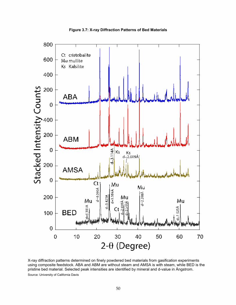
Figure 3.7: X-ray Diffraction Patterns of Bed Materials

X-ray diffraction patterns determined on finely powdered bed materials from gasification experiments using composite feedstock. ABA and ABM are without steam and AMSA is with steam, while BED is the pristine bed material. Selected peak intensities are identified by mineral and d-value in Ångstrom. Source: University of California Davis

50

The unused bed material is composed mainly of a mixture of cristobalite and mullite in addition to small amounts of rutile. The used bed materials are likewise as expected dominantly composed of cristobalite and mullite, which do not suffer any detectable transformations and reactions during firing, irrespective of the addition of a water steam to the reactor. Only for the firing with an addition of water steam does reactions occur in sufficient amounts to de clearly detected. This is seen for the AMSA steamed bed where kalsilite result from a reaction between mullite and the potassium laden flue gas. The dry firing results in much less kalsilite at or below the detection limits for the X-ray diffraction method (ABM and ABS).

SEM imaging was conducted on used bed materials from after air gasification runs. Figure 3.8 and Figure 3.9 display typical images of used bed material after a reaction run under air gasification conditions with almond biomass as the feedstock. Some light corrosion was seen along the edges of most typical bed particles. Corrosion zone was determined to be composted of a mixture of kalsilite and mullite.

Figure 3.8: SEM BSE Image of Used Bed Material

SEM BSE image of typical used bed material exposed to air gasification of almond biomass. The light rims of corroded bed particles are observed around most sand particle. The grey scale reflects the mean atomic density of mainly Si, Al, and K and the scale bar is 500 μm. Source: University of California Davis

51

Figure 3.9: Higher-Resolution SEM BSE Image of Bed Material

SEM BSE image of typical used bed material exposed to air gasification of almond biomass. The light corroded zone occupies most of the bed particle made up of a mixture of kalsilite and mullite. The grain is 100 μm. Source: University of California Davis

X-ray Kα density maps for Si, Al, Ti, and K have been developed as seen in Figure 3.10 and Figure 3.11. Potassium containing elements were found to collect on the surface of bed materials. Titanium was also found in concentrated regions inside the bed particles. Elemental composition of spent bed material is given in Table 3.7.

52

Figure 3.10: SEM BSE Image of Bed Material for Detailed Analysis

SEM BSE image of typical used bed material exposed to air gasification of almond biomass. The center grains are illustrated in Figure 3.11. The grain is 500 μm. Source: University of California Davis

53

Figure 3.11: X-ray Kα Density Maps

X-ray Kα density maps for Si, Al, Ti, and K. top left: topography; top center: BSE mean atomic density; top right: Si, bottom left: Al, bottom center: Ti, and bottom right: K. The scale bar is 200 μm.


Table 3.7: Composition of Bed and Rims


54

3.3.3.2 Gravimetric Tar Study Results Investigation of tar sampling nozzle after sampling indicated proper performance of the recirculation system. Continuous solvent recirculation resulted in a very clean inner surface in contrast with the tar covered exterior of the nozzle (Figure 3.12).

Figure 3.12: Pictures of Sampling Nozzle

Photo Credit: University of California Davis

Comparison of resulting tar concentrations between the two methods (Gravimetric and SPA) indicate almond biomass derived producer gas contains contaminate tars near the expected concentration; though some disagreement exists between methods (see Table 3.8).

Table 3.8: Gravimetric Tar Analysis Results

Sampling Date

Gravimetric Sampling Results [g/Nm3]

Solid Phase Adsorption (SPA) Results [g/Nm3]*

Standard Results [g/Nm3]**

3/17/15 12.08 15.20 ± 1.05 7-10 4/3/15 7.93 ± 0.27*** 16.69 ± 0.54 7-10 4/10/15 12.67 10.79 ± 2.98 7-10 *SPA samples taken in triplicate; results given as μ±2σ **Source: Milne, 1998 ***Analysis was run in triplicate; results given as μ±2σ Source: University of California Davis

55

Triplicate analysis of gravimetric method solvent, though time consuming, does indicate repeatability of the gravimetric analysis method. Further investigation into tar and tar sampling method is currently underway.

After completion of the commercial pilot-scale BCHP system construction and commissioning, a number of test runs were conducted over a period of months to collect data on the performance of the system. This chapter discusses these tests. The performance of the BCHP system in conversion of the agricultural biomass feedstock to combustible gas for power production and heat utilization was demonstrated relative to the stated efficiency and other performance objectives.

3.4 BCHP Process As described in detail in Chapter 2: Design and Installation of the BCHP System, the BCHP process is based on gas production via gasification in an FICFB reactor system. The FICFB reactor system generates product gas from biomass via an indirect-heated bubbling-bed gasifier that is fluidized with steam and heated with hot bed material that is continuously circulating from an integrated fast-fluidized combustion reactor. Char that consists of fixed carbon from the biomass is circulated from the gasifier to the combustion reactor where it is oxidized and provides heat for the process. Supplemental fuel can also be supplied, if required, to the combustion zone to increase the heat to the gasifier. The FICFB process generates a product gas and flue gas stream that are additionally processed for heat recovery and cleanup. This processing includes a heat recovery loop including multiple heat exchangers that recover heat to the input air and steam and can provide excess heat for utilization. The product gas is filtered and scrubbed in order to prepare it for utilization in an engine generator system. The filtered particulate matter and condensate from the scrubber system are recovered to the process. The flue gas is also filtered for removal of ash particles and run through an adsorber bed for trace gas filtration before being vented via a stack.

The complete FICFB system is controlled by an advanced supervisory control and data acquisition system (SCADA) system that monitors the multiple components of the system during operation and controls the operation of the equipment using variable control valves and variable frequency drives. Figure 4.1 shows some views of the control room with the panel of drives that control all of the process equipment and the operator panels that show the SCADA interface used by the operator to monitor the process. There are a number of types of sensors used by this system including thermocouples, pressure transducers, gas and water flowmeters, electronic scale systems, level sensors, gas analyzers, and others. Several of these sensors are shown on the plant in Figure 4.2. The location of the sensors is included in the following section that describes the monitoring systems used during the test runs to monitor the performance of the BCHP system.

56

Figure 4.1: Motor Drive Systems (left) and SCADA Operator Interface (right) in BCHP Control Room

Figure 4.2: Various Sensor Systems Utilized to Monitor and Control the BCHP Process

3.5 Materials and Methods In order to monitor the process during the test runs on agricultural biomass, the data from the SCADA system which includes all of the sensors and all of the equipment set-points (valves and motor drives) was recorded on a continuous basis. The SCADA system monitors thermocouples, pressure transducers, oxygen sensors, flow meters, and ultrasonic level sensors at each subsystem. The SCADA system also controls pneumatic valves are used to set the flowrate of super-heat steam, air and compressed hot water of the system. A total of 18 variable

57

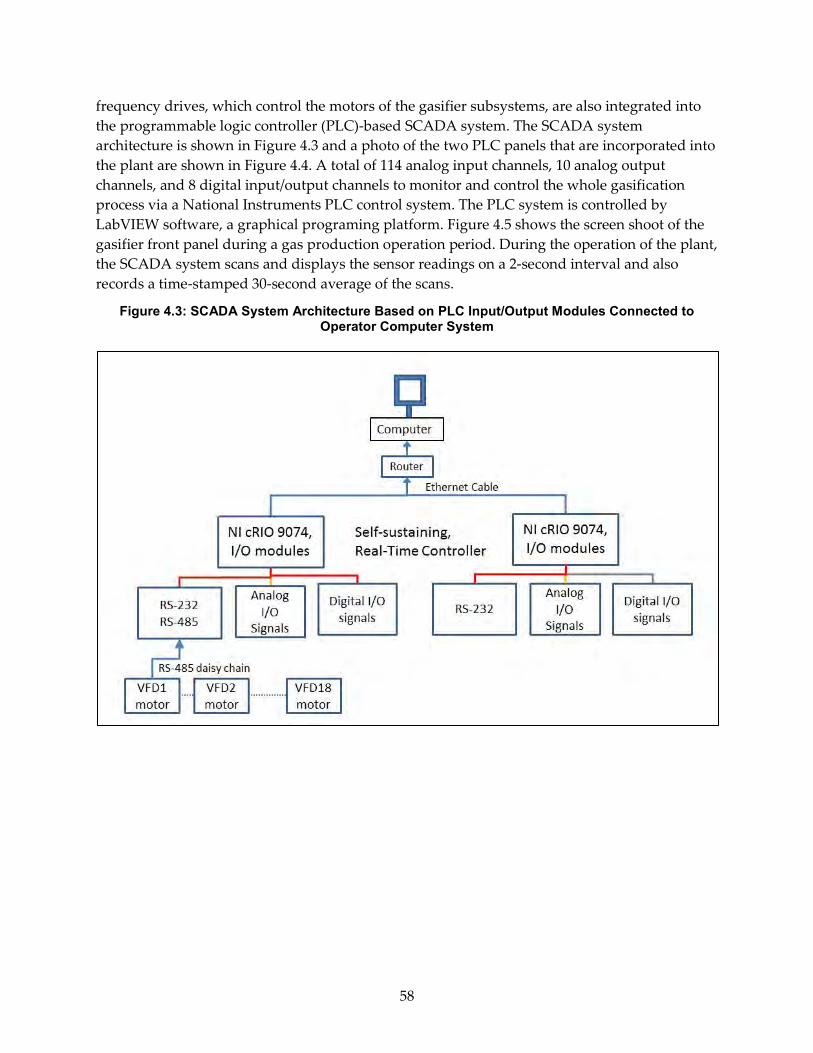
frequency drives, which control the motors of the gasifier subsystems, are also integrated into the programmable logic controller (PLC)-based SCADA system. The SCADA system architecture is shown in Figure 4.3 and a photo of the two PLC panels that are incorporated into the plant are shown in Figure 4.4. A total of 114 analog input channels, 10 analog output channels, and 8 digital input/output channels to monitor and control the whole gasification process via a National Instruments PLC control system. The PLC system is controlled by LabVIEW software, a graphical programing platform. Figure 4.5 shows the screen shoot of the gasifier front panel during a gas production operation period. During the operation of the plant, the SCADA system scans and displays the sensor readings on a 2-second interval and also records a time-stamped 30-second average of the scans.

Figure 4.3: SCADA System Architecture Based on PLC Input/Output Modules Connected to Operator Computer System

58

Figure 4.4: SCADA System PLC Panels on the BCHP Plant

Figure 4.5: SCADA System Front Panel

The types of sensors utilized in the plant and recorded by the SCADA system are described in Table 4.1. The locations of the various sensors are shown in Figure 4.6 through Figure 4.12 with the label “T” showing locations of thermocouples, “P” showing locations of pressure transducers, “F” showing locations of flowmeters, and “L” showing the location of level sensors. A more complete description and detailed listing for each sensor is included in Appendix A. The manufacturer operating, maintenance, and calibration procedures were followed for these sensors.

59

Table 4.1: Sensors Used in SCADA System to Monitor the BCHP Operation and Performance

Sample/Measurement Method Location/Details 5 Gasifier temperature (°C) 10 Combustor temperature (°C) 12 Clean-up system temperature (°C) 25 Heat recovery system temperature (°C)

K-type thermocouple continuously monitored by LabView DAQ system

Various locations on gasifier Various locations on combustor Various locations on clean-up stream Various locations on heat recovery system

Gasifier/Combustor pressure (millibars [mBar], gage) Reactor cross-bed differential pressure (DP) (mBar, differential) Filter housing DP (inches water column [“WC], differential) Scrubber DP (“WC, differential) Hot water pressure (pounds per square inch, gage [psig]) Steam and hot air pressure (pounds per square inch, absolute [psia])

Gage pressure transducer, monitored by LabView DAQ system Differential pressure transducer, monitored by LabView DAQ system Differential pressure transducer, monitored by LabView DAQ system Gage pressure transducer Absolute pressure transducer

Various locations on gasifier and combustor sides Locations above and below the bed on gasifier and combustor Gasifier and Combustor filter housings’ inlet to filter housings’ outlet, DP Scrubber inlet to scrubber outlet, DP Recovery heat system hot water lines Various locations on steam and hot air lines

60

Sample/Measurement Method Location/Details Fluidizing air flow rate (kilograms per second [kg/s]) Fluidizing steam flow rate (kg/s) Flue gas flow rate (kg/s) Syngas flow rate (kg/s) Hot water flow rate (L min-1) Nitrogen (N2) flow rate (liters per minute [L min-1]) N2 flow rate (L min-1) Steam make-up water flow rate (L min-1)

Pitot tube via DP transducers monitored by LabVIEW DAQ system Ultrasonic flow meter Mass flow meter Anemometer Vortex flow meter

Combustor air lines Steam generator, Gasifier, & cyclone steam lines Combustor flue gas line Gasifier downstream line Heat recovery line Feeder screw box Gasifier bag house Water inlet of steam generator

Biodiesel level sensor (inch) Condensate water level sensor (inch)

Ultrasonic level sensor connected to LabVIEW DAQ system

Scrubber settlement tank

Feedstock mass (kg/lb)

Floor scale monitored via RS232 to LabVIEW DAQ system

Feedstock weighed rea-time during operation

Gasifier/combustor oxygen sensor (%) Back-up oxygen sensor (%)

Paramagnetic oxygen analyzer monitored by LabVIEW DAQ Zirconia type oxygen analyzer

Locations on gasifier and combustor downstream lines

Gas composition (% by vol) Gas composition (% by vol)

CH4, CO, CO2, C6H6, C7H8, C10H8 by on-line FTIR H2, CH4, N2, CO, CO2, on-line or of grab samples by gas chromatography

Sampling after the clean-up system Sampling before or after the clean-up system

Tar concentration and composition (grams per cubic meter [g m-3], % by vol) Tar concentration (g m-3, % by vol)

Gravimetric by BSI – 15439:2006 tar standard SPA

Sampling before or after the clean-up system

61

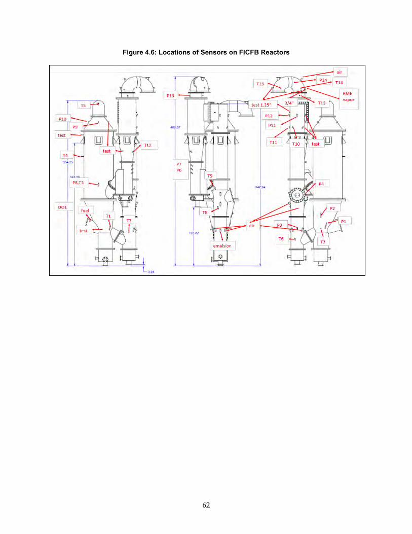
Figure 4.6: Locations of Sensors on FICFB Reactors

62

Figure 4.7: Locations of Sensors on Heat Recovery System

Figure 4.8: Locations of Sensors on Steam Generator System

63

Figure 4.9: Locations of Sensors on Product Gas Filter System

Figure 4.10: Locations of Sensors on Product Gas Scrubber System

64

Figure 4.11: Location of Sensors on Product Gas Handling System

Figure 4.12: Locations of Sensors on Flue Gas Handling System

65

The test runs took place during late 2014 and early 2015 and consisted of a cold plant startup, operation with agricultural biomass, and a complete plant shutdown back to cold condition. Five multi-day test runs were completed during this time period and all sensor data was recorded by the SCADA system for the entire operating period. Post-processing of the data included calculating weighted averages over a time periods of stable operation to determine energy and mass balance relationships. More details of the testing procedures are contained in BCHP System Performance Test Plan in Appendix B.

3.6 Results and Analysis The startup of the gasifier system requires the use of an external fuel in the combustor to bring the fluidized bed up to operating temperatures. A propane burner was installed on the combustor side to start the process and then propane can be combusted in the combustor bed once auto-ignition temperature has been reached. Figure 4.13 shows the gasifier bed temperature profile of the five test runs, during the start-up period. The system takes about 30 hours to heat up to the proper gasifying temperature of 850 °C. The first six to eight hours is spent heating the reactor and then bed circulation starts and the gasifier also heats up via the circulating bed material. Once the system enters into the circulation mode, the gasifier temperature jumps from ambient temperature to 600°C. It takes another 19 to 20 hours to heat the gasifier to 850°C for gasification to begin.

Figure 4.13: Gasifier Bed Temperature During Plant Start-Up

The differential pressure across the bed inside the gasifier is a parameter that indicates that the bed is fluidized and also indicates the total volume of the fluidized bed. During the circulation mode, the gasifier bed starts bubbling fluidization. An ideal cross-bed differential pressure of

66

between 80 and 120 mBar is ideal for the gasifier. Figure 4.14 shows the differential pressure across the gasifier bed during start-up for the five test runs. The fluidized state is restricted by the steam and recycled gas flow rate injected at the bottom of the gasifier.

Figure 4.14: Differential Pressure Across the Gasifier Bed during Start-Up

The amount of external fuel consumed for starting up the plant is an important parameter for understanding the energy balance and operating costs. The metered propane used for plant start-up is shown in Figure 4.15. Table 4.2 shows the rate and amount of propane usage required for the test runs. It takes between 43,000 to 50,000 megajoules (MJ) of propane was used to heat up the system at rates from 0.40 – 0.45 MWth.

67

Figure 4.15: External Fuel Metering During Plant Start-Up

Table 4.2: External Fuel Consumption for Start-Up of BCHP Plant

Fuel usage (Propane) Test1 Test2 Test3 Test4 Test5 Total Fuel Required (MJ) 43,706 49,748 49,790 49,124 48,870 Average Heat Rate (MW) 0.440 0.396 0.451 0.447 0.451

Once the plant achieved the temperature conditions for gasification, the introduction of biomass began. During this transition from external fuel to biomass, the recycle of gas is eliminated so that the gasifier was only fluidized with steam and the external fuel is gradually reduced as char begins to circulate to the combustor zone. During each of the five tests, product gas was produced from agricultural biomass and the heat and mass balance of the process was analyzed once stable conditions were achieved. Runs with different combinations of testing conditions were tried during these tests to become familiar with the optimal conditions to operate the plant. For the analysis here, six of these runs with similar operating conditions were analyzed to show the performance of the plant. Table 4.3 shows the operating condition ranges that were focused on for the analysis of plant performance on agricultural biomass with maximum and minimum values as well as a time weighted average over the course of the runs.

68

Table 4.3: Operating Conditions for Agricultural Biomass Test Runs in Woodland BCHP

Parameter Min Max Weighted Average

Biomass Feedrate (kg/hr) 170.6 185.3 182.2 Biomass Gross Heat Rate, Lower Heating Value (LHV) (kW) 732 795 781

Gasifier Bed Temperature (°C) 802 875 849 Combustor Bed Temperature (°C) 890 1008 942 Air to Combustor (kg/hr) 717.8 791.9 766.0 Steam to Gasifier (kg/hr) 58.7 91.4 69.0 Steam to Biomass Ratio (-) 0.32 0.54 0.38

During gas production, the gasifier was able to be maintained at a stable temperature with a small introduction of supplemental fuel. This is due, in part, to the fact that the recycling of filtered char and scrubber oil to the combustor had not been fully integrated for these tests. However, the geometry of this small-sized pilot also means a somewhat higher heat loss than that a larger commercial sized plant, so more heat is required from the combustor to maintain the same temperatures. This is analyzed more fully in the modeling section. The pressure across the gasifier and combustor beds were also maintained in optimal conditions of approximately 100 mBar which is consistent with a bed height of about one meter and is consistent with how the FICFB in Austria is maintained. Figure 4.16 shows the stable operating conditions of the Woodland FICFB during one of the gas producing test runs in comparison with results reported from the Güssing FICFB and it can be seen that very similar operating conditions were achieved.

69

Figure 4.16: Operating Conditions From Woodland FICFB (top) and Güssing FICFB (bottom)

The composition of the product gas that was produced by the FICFB showed to be consistent with the gas produced in the commercial plant in Güssing. Table 4.4 shows the gas composition ranges that were achieved using agricultural biomass over the test runs in comparison with typical ranges for the reference commercial plant.

70

Table 4.4: Product Gas Composition From Woodland FICFB in Comparison With Güssing FICFB

Gas Composition (wet basis) Min Max Average

Güssing FICFB Range

(Weber, 2013)

H2 (vol%) 30.03% 39.63% 33.48% 35% - 45%

CO (vol%) 20.32% 28.97% 26.28% 19% - 23%

CO2 (vol%) 14.96% 19.57% 16.07% 20% - 25%

CH4 (vol%) 5.38% 11.34% 8.27% 9% - 11%

C2H4 (vol%) 0.87% 2.69% 1.87% 2% - 3%

C2H6 (vol%) 0.13% 0.48% 0.28% ~0.5%

C3H8 (vol%) 0.01% 0.04% 0.02% ~0.01%

N2 (vol%) 2.09% 8.35% 6.26% <2%

O2 (vol%) 0.00% 0.93% 0.34% <0.1%

C6 + C7 (vol%) 0.05% 0.27% 0.13% <0.09%

LHV [MJ/kg] 10.98 14.16 12.60 11.0 – 13.0

In terms of gas production and the overall energy performance of the BCHP during the test runs on agricultural biomass, the results show a good overall performance relative to the project goals. Table 4.5 shows the energy inputs and outputs and the recovered energy flows from the various process units relative to their designed values. Overall the efficiency objective of the gasifier was achieved, even considering the supplemental fuel. If the supplemental fuel can be eliminated in a commercial plant, with its lower reactor heat losses and by using scrubber and filter recycle to the combustor, a higher gasifier efficiency of 81.4% can be achieved. The projected electrical efficiency of using the product gas in a lean-burn engine generator (assumed 35% efficiency) was 22.8% considering the supplemental fuel and 28.5% without supplemental fuel, which shows that the efficiency objective was also achieved.

71

Table 4.5: Energy Flows of Process Units During Gas Production Runs of Woodland BCHP

Parameter Min Max Average Design Values

Biomass Gross Heat Rate, LHV [kW] 732 795 781 700-1000

Supplemental Fuel Heat Rate, LHV [kW] 0 438 193 0-450

Heat Recovered to Air Preheat [kW] 62 78 68 70

Heat Recovered to Steam Generator [kW] 82 114 107 150

Heat Recovered to Steam Superheat [kW] 19 28 23 20

Excess Heat Recovered to Hot Water [kW] 181 239 214 0-250

Cold Gas Heating Value, LHV [kW] 580 650 636 550-800

Net Heat Loss [kW] -44 351 125 150

Cold Gas Efficiency (biomass only) [%] 79.2% 83.1% 81.4% 75%

Cold Gas Efficiency (all inputs) [%] 49.6% 81.1% 65.2% 65%

Gross Overall Efficiency (gas + heat) [%] 69.5% 105.6% 88.0% 85%

Further results and details for all of the plant test runs are contained in Appendix B.

72

CHAPTER 4: Emission Control Systems Performance In order to demonstrate that the BCHP system can achieve CARB standards for small power generation systems, two emission control systems were designed and tested: an adsorber with microwave regeneration for the combustor flue gas exhaust and a compact selective catalytic reduction (SCR) system for the engine exhaust.

4.1 Flue Gas Adsorber System with Microwave Regeneration An adsorber was designed to remove NOx, VOC, and sulfur dioxide (SO2) from the combustion flue gas generated by the gasifier. The adsorption media will be selected to remove NOx, VOC, and SO2 from the combustion gas without early breakthrough and a microwave system will be used to regenerate the adsorbent without emissions to the environment.

4.1.1 Background CHA Corporation (CHA) has successfully completed several field demonstration of microwave regenerable adsorbent technology to remove and destroy NOx, SO2, and VOCs from engines or other exhaust gases. Under CARB’s 1996 Innovative Clean Air Technologies (ICAT) program, CHA teamed with the Sacramento Municipal Utility District (SMUD) and the former McClellan Air Force Base in 1998 to successfully demonstrate the use of carbon adsorption with an onsite microwave regeneration and treatment system to remove NOx, VOC, CO and coarse particulagte matter (PM10) emissions from a diesel engine at McClellan Air Force Base. The demonstration was successful at reducing over 1,000 ppm of NOx in the diesel engine exhaust to a concentration of about 1ppm. Based on the results of this demonstration and further developments by CHA, an exhaust treatment for use on biogas engines has been developed that has the potential to meet or exceed performance of existing technology and meet CARB 2007 standards for stationary generators for NOx, SOx, and VOC.

In 2009, CARB awarded SMUD an ICAT grant to remove H2S from biogas and NOx from an IC engine running on biogas. As SMUD’s subcontractor, CHA conducted a field demonstration at Tollenaar Holsteins Dairy in Elk Grove, California to remove NOx from their 212 kW IC engine and H2S from biogas. CHA used magnesium oxide (MgO)-impregnated activated carbon to remove NOx and a 6-kW moving microwave applicator to regenerate media in place. Testing proved the ability to remove NOx to levels below 5 ppm. However the economics of the in-situ regeneration process were not favorable, with an estimated cost of $0.031/kWh. The high generation cost is due to the added capital cost of the regeneration equipment. An economic assessment of central regeneration system serving multiple adsorption sites estimated the cost could be reduced to $0.011/kWh.

CHA completed several field demonstrations of microwave regenerable adsorbent technology to remove VOC and hydrocarbon solvent vapors in air. The McClellan Air Force Base awarded a grant to CHA to conduct a 3-month field pilot plant testing of microwave system with the onsite regeneration at the former McClellan Air Force Base in 1999 to remove and destroy VOC and chlorinated solvents from soil vapor. This demo was successful in removing and destroying

73

chlorinated solvents from soil vapor. Under the Small Business Innovation Research (SBIR) Phase I awarded by the National Institute of Health, CHA conducted 4-month field-testing of microwave prototype at McClellan Park to recover hydrocarbon and chlorinated solvents from soil vapor. Thirteen cycles of adsorption and microwave regeneration were successfully completed to recover 10-12 kg/hr hydrocarbon liquid, mainly JP-4 fuel. After 13 cycles, the mass of liquid recovered hourly did not decrease, indicating that microwave regeneration restored the carbon adsorption capacity. Also, CHA built and demonstrated a 100-lb/hr mobile microwave unit at McClellan Park for two weeks in 2006. Under the Energy Commission’s Public Interest Energy Research (PIER) grant awarded to SMUD, this microwave mobile unit was again used to conduct a field demonstration of microwave technology to remove siloxanes, hydrocarbon, and H2S from biogas at Carson Energy in Elk Grove, California. Furthermore, CHA microwave regenerable adsorbent technology has been demonstrated successfully at Tyndall Air Force Base, Edwards Air Force Base, and Montana State University to remove and recover or destroy chemical vapors from air (CHA Corporation, 2014).

4.1.2 Materials and Methods The NOx control system consists of two distinct units. The first part is the NOx adsorption system. This consists of a heat exchanger and an activated carbon adsorber. Figure 5.1 shows the process flow diagram for the adsorption system.

Figure 5.1: Adsorption Process Flow Diagram

The Exhaust Gas Cooler is a custom built aluminum gas-to-liquid heat exchanger supplied by Martin Machinery Company (Figure 5.2). The Carbon Adsorber is a TetraSOLV VFV-1000 steel adsorber (Figure 5.3) that has a capacity of approximately 1000 lbs of Activated Carbon. Type J

74

thermocouples were used for temperature measurement, with the data being logged with IOtech DAQBook 260 data logger. NO, NO2, CO, and SO2 concentrations in the inlet and outlet to the adsorber were sampled using a Testo model 350XL combustion gas analyzer.

Figure 5.2: Exhaust Gas Heat Exchanger

75

Figure 5.3: Carbon Adsorber

The Second part of the process is the Microwave Carbon Regeneration System. This system was originally built under a National Institute of Environmental Health Sciences SBIR Phase II grant. The Process Flow Diagram for the system is shown in Figure 5.4. Figure 5.5 is a photo of the Microwave Regeneration Tower, and Figure 5.6 is a photo of the two microwave reactors used to process the sweep gas.

76

Figure 5.4: Microwave Regeneration Process Flow Diagram

77

Figure 5.5: Trailer-Mounted Carbon Regeneration Unit

78

Figure 5.6: Microwave Destruction Reactor Skid

The test procedure involves loading the adsorber with a measured mass of adsorption media. During gasifier operation the exhaust gas from the combustor is directed through the heat exchanger to reduce the temperature from ~120°C to below 50°C. The cooled gas then passes through the adsorber where the media removes NOx and SO2. The exhaust exits the adsorber and returns to the existing stack.

Following operation the used media is removed from the adsorber using a vacuum system and weighed. The adsorbent is then transferred to the microwave regeneration unit for processing.

79

The weight is measured after regeneration before the adsorbent is transferred back to the adsorber for reuse.

4.1.3 Results and Analysis Due to a problem receiving the adsorber from the supplier, only one test cycle was run on the NOx removal media. For this test the adsorbent media used was a magnesium oxidempregnated activated carbon supplied by Siemens. Due to the limited number of runs available for testing, media that had been used previously to remove NOx during ICAT testing at Tollenaar was selected to simulate the response of media that had been used for a number of cycles. This media had been subject to six previous saturation-regeneration cycles during the previous ICAT testing. It was also decided to reduce the media load in the adsorber to ~500 lbs to shorten the saturation time.

Initial shakedown testing of the adsorption system was performed February 19, 2015. Testing was performed by heating only the gasifier combustor with propane and passing the exhaust to the adsorber. Two problems were encountered during this test. First, the pressure drop through the adsorber was too high for the exhaust gas blower to divert 100% of the exhaust gas flow through the media. The second problem was that very early in the test, NOx was observed in the adsorber outlet. To address the pressure drop problem, openings in the adsorber gas distribution manifold were enlarged. Then the bottom of the adsorber was filled with large diameter aggregate and a new screen to prevent the adsorption media from falling into the holes. Because the media was used and had been in storage it was processed through the Microwave Regenerator to improve the adsorption properties.

Following these changes the Adsorption System was tested again by firing the combustor with propane on February 26, 2015. During this test the flow through the adsorber was only increased slightly. However the regenerated media did perform well during the test, reducing the average inlet NOx concentration from 42 ppm to 1.3 ppm for the duration of the test.

Because the media used during the shakedown test was only used for a short period of time, it was left in the adsorber for use during the next full gasifier run. The run was started March 9, 2015 with exhaust flow diversion to the adsorber occurring at 20:10 (8:10 pm local time). The NOx concentration in the outlet began increasing after 1 hr, reaching 5 ppm by 21:30. To conserve the bed capacity the flow to the adsorber was shut off at 23:15 to wait until biomass processing started.

Biomass loading began March 10, 2015 at 13:20. At this time 50% of the exhaust flow from the combustor was diverted to the adsorber. Due to problems with biomass feeding during the duration of the test, the flow to the adsorber was never increased beyond 50%. Even at the reduced flowrate, the NOx concentration in the outlet increased to 20 ppm within an hour. For the remainder of the test, the outlet remained roughly in this range. There were periodic spikes of SO2 observed in the inlet gas, likely coinciding with feeding operations. The SO2 in the adsorber outlet remained non-detectable throughout the test. Figure 5.7 shows the inlet and outlet contaminant concentrations recorded during the test and Table 5.1 summarizes the results.

80

Figure 5.7: Contaminant Concentration from Gasifier Run 3/9/15

Table 5.1: Summary of Adsorber Contaminant Removal

Contaminant Average Inlet (ppm)

Average Outlet (ppm)

Removal (%)

NO 42.7 23.8 44.2

NO2 1.5 ND 100

SO2 2.5 ND 100

After the test, the media was regenerated using the microwave regeneration equipment. The throughput was much lower than expected due to two factors. The media adsorbed a large amount of water during saturation, which requires more energy to remove. The media was also beginning to physically break down. The loss of mechanical integrity results in more fine particles in the regenerator, which leads to plugging and loss of material flow. Despite these issues, the material was regenerated over a period of 7 days and the media weights were recorded. Table 5.2 summarizes the results of the regeneration.

0.0

50.0

100.0

150.0

200.0

250.0

300.0

350.0

400.0

3/9 18:00 3/10 0:00 3/10 6:00 3/10 12:00 3/10 18:00 3/11 0:00 3/11 6:00

Conc

entr

atio

n (p

pmv)

Date/Time

Contaminant Concentrations

Inlet NO

Inlet NO2

Inlet SO2

Outlet NO

Outlet NO2

Outlet SO2

Shut down Adsorber DuringWarmup to Collect Data During Biomass Processing

81

Table 5.2: Summary of Weights From Regeneration

Media Starting Weight (lbs) 326.9

Weight After Adsorption (lbs) 381.5

Weight After Regeneration (lbs) 308.0

Water Recovered During Regeneration (lbs) 43.5

Carbon Fines Recovered From Transfer Cyclone (lbs) 13.7

4.1.3.1 Conclusions The previously regenerated MgO media used in this test did not meet our performance goal. The fact that NOx levels increased early in the test, but remained stable around 20 ppm for the duration of the test indicates that the adsorber bed geometry may be a limiting factor, rather than the media becoming fully saturated. Because the carbon adsorption of NOx requires that the NOx be in the form of NO2, the rate of conversion of NO to NO2 can have a limiting effect on removal efficiency. Although at low temperature the equilibrium favors NO2 formation, the rate of the reaction can be slow depending on gas composition. It appears that the reduced bed depth didn’t provide sufficient residence time to convert the NO to NO2.

We recommend running additional tests with increased media amounts to determine whether the residence time is the limiting factor.

4.2 Compact Selective Catalytic Reduction System The synthetic gas produced by the reactor was piped to a modified natural gas engine for power production or to a flare for disposal. In the gas engine, the fuel was burned under lean conditions to generate electricity. Lean-burn engines are inexpensive, highly efficient, and have excellent turn-down capability but produce relatively high emissions of NOx and VOC. Due to the high CO content of the fuel, it was anticipated that CO emissions from this engine would also be relatively high. An emission control system would therefore be required.

The emission control system used with this engine was a Compact SCR™ system supplied by Engine, Fuel, and Emissions Engineering, Inc. SCR is a highly-effective NOx control technology for lean-burn engines. The SCR catalyst used in the Compact SCR™ systems was also effective in oxidizing VOC emissions to CO. A separate platinum catalyst was used to promote the oxidation of CO to CO2 and to provide additional VOC oxidation.

4.2.1 Background Lean operation of the engine lowers the emissions of NOx through colder combustion temperatures. Once the engine is operated above a certain value of air-fuel equivalence ratio, Lambda, NOx emissions decrease as a function of Lambda. Figure 5.8 shows NOx emissions that were obtained on two different types of producer gas on a single-cylinder laboratory test engine. Blend 1 contained, by volume, 40% H2, 24% CO, 23% CO2, 10% CH4, and 3% C2H4. Blend 2 contained 33% H2, 31% CO, 23% CO2, 10 CH4, and 3% C2H4. Also shown in Figure 5.8 is that

82

there is a lean limit beyond which the engine cannot be easily operated at. The lean limit is reached when the combustion becomes unstable from cycle to cycle and this can be expressed in coefficient of variation (COV) of net mean effective pressure (NMEP), for example stipulating that this value should not exceed 5%. Larger values would prevent smooth operation of the engine, and misfire can occur when the engine is operated even leaner.

During normal operation of multi-cylinder engines on syngas fluctuations in fuel supply, either in quantity or in composition may occur. There may also be a variation across the different cylinders so that some could experience earlier misfire than others. Both factors lead to the effect that the engine will need to be operated on average slightly richer than the lean limit, which in turn increases NOx emissions. A well-tuned engine and control program are important factors for lean-burn engines.

Figure 5.8: Test-Engine Emissions as a Function of Air-fuel Equivalence Ratio, Lambda

Brake-specific NOx emissions at lean operation. Open symbols represent data points beyond the lean limit (> 5% COV NMEP). The indicated NOx numbers are at the projected lean limit. NMEP was held constant at 10 bars, and the compression ratio was 9.6. Source: University of California San Diego

For a given level of engine-out NOx emissions, SCR can reduce the tail-pipe emissions to meet air-quality requirements. SCR works by adding a small amount of a reductant chemical to the exhaust upstream from a catalytic converter. Commonly-used reductants are ammonia and

83

urea (which breaks down to form ammonia in the hot exhaust). The catalyst in the converter selectively promotes the chemical reaction between the ammonia and the NOx. This reaction converts both the ammonia and the NOx into harmless nitrogen gas and water vapor. Common SCR catalysts include vanadium oxide and various zeolites. The catalyst used in this project was a mixture of vanadium, titanium, and tungsten oxides.

The amount of reductant needed for NOx control varies with the amount of NOx in the exhaust. Too little reductant means that some NOx escapes un-reacted, while too much means leftover ammonia in the exhaust (ammonia “slip”). In the Compact SCR™ systems, a programmable controller varies the reductant injection rate to match the NOx emission rate from the engine. A metering pump injects the right amount of reductant into a stream of compressed air going to an atomizing nozzle in the exhaust. The compressed air cools the nozzle, keeps the reductant from caking, and aids in atomization. Urea is injected into and mixes with the recombined exhaust stream before it enters the SCR catalyst, where the reactions take place to convert NOx to N2 and water.

The programmable controller includes solid-state NOx sensors upstream and downstream of the SCR catalyst to enable self-tuning. The control method employs both feed-forward and feed-back control. In the feed-forward aspect, controller responds to changes in the exhaust flow rate (as indicated by engine load) and in the NOx concentration of the exhaust stream. In the feed-back aspect, the controller “learns” and remembers the optimum urea injection rate to minimize NOx and ammonia emissions at each engine load point.

4.2.2 Materials and Methods Table 5.3 lists the main parameters for the engine configuration. To provide feedback control for the air/fuel ratio, wide-band sensors are used. Relying solely on this type of control in connection with a PID controller is not optimal because there is a delay of a few seconds between the command to the control valves and the measurement of the new Lambda value. If the proportional as well as the integral parameters in the PID controller are too large, they will lead to oscillations. Oscillations near the lean limit in a lean-burn engine, affect how lean the engine can be operated and need to be. The derivative parameter of the PID controller is subject to noise and therefore not useful in this configuration.

The solution to achieve better engine control is to combine the feedback controller with a feed-forward controller. The feed-forward controller is derived from an engine process model. It estimates the position of the air-control valve based on the desired power, Lambda, and measured fuel flow rate. The feedback controller is then only used to correct errors in the process model and can use smaller proportional and integral parameters. Figure 5.9 shows a simplified diagram of the control system. If the fuel flow from the gasification plant increases or the operator changes the engine load, the feed-forward controller can calculate a new air-valve position. This calculated position is combined with the correction of the PID controller and then sent to the hardware adjusting the valve. Based on the new engine load, fuel pressure, and air-valve position, the engine will attain a new operating condition. If the measured Lambda value is different from the Lambda setpoint, the feedback controller will adjust the air-valve correction and this will update the valve position.

84

Table 5.3: Engine Configuration

Parameter Value

Engine Model Waukesha H-2475G

RPM 1200

Compression Ratio 9.41

Bore 7.5"

Displacement 40.5 L

Type V8

Generator Power 0-200 kW

Ignition Timing 21 deg BTDC

Spark Plugs Altronic Pre Chamber P1863DP

Lambda Sensors Innovate LC-2 Wideband

RPM Control Electronic Governor

Lambda Control Feed-forward/Feedback Control of Air Valve


Figure 5.9: Schematic of Engine Control System


The process model is written in a procedural language inside a calculator block with the Labview control program. The model uses a combination of estimated and measured engine fuel flow. Combined with the engine load and fuel pressure, the pressures in the intake and the

+

-

Waukesha Engine

Feedback Controller (PID)

Lambda Sensor

++

Feed-forward Controller (Process Model)

Stoichiometry

Final air-valve position

Air-valve correction

Predicted air-valve position

Lambda Setpoint

Measured Lambda

Load Setpoint, Fuel Pressure, etc.

85

main-throttle position are estimated. (The actual throttle-position is controlled by the governor included in the engine setup). From these values, the pressure at the fuel/air mixing tee can be estimated, and together with the calculated air flow (from Lambda and fuel flow), the air-valve position can be calculated.

In order to determine some of the necessary operational parameters of the Waukesha engine, some preliminary tests were conducted on a mixture of propane (18% by volume) and nitrogen (82% by volume). This mixture has a LHV of 11.8 MJ/kg (16.2 MJ/Nm3). The mixture was created by using two needle valves and estimating the flow rates from the valve flow coefficient values. The mixture was then analyzed using a micro-gas chromagraph. The intake-manifold pressure was measured for various levels of power and Lambda. From the intake pressure and Lambda, the thermal energy of the intake charge can be calculated. The relation of the electrical power to the thermal energy of the fuel is the engine efficiency and is one of the major parts of the engine model. Table 5.4 shows the results for some of the operational points on the propane/nitrogen mixture. It shows that for leaner fuel/air mixture and larger power, the intake pressure rises and nears un-throttled operation (~1,000 mbar). Producer gas contains large amounts of hydrogen and is expected to burn better than the propane in lean mixtures and reach larger values of Lambda. For the propane/nitrogen mixture, only Lambda values up to 1.34 were used. The results also show some preliminary values of emissions before and after the SCR and oxidation catalyst during the developmental phase. The SCR operation was not optimized yet, but shows that for Lambda 1.34 and 151 kW, NOx was reduced from 116 ppmv to 30.4 ppmv. The oxidation catalyst reduced CO by more than 50%.

Table 5.4: Engine Operation on a Propane/Nitrogen Mixture

Lambda Power Intake pressure

NOx (engine-out)

NOx (tailpipe)

CO (engine-out)

CO (tailpipe)

O2 (engine-out)

O2 (tailpipe)

[kW] [mbar] [ppmv] [ppmv] [ppmv] [ppmv] [vol%] [vol%]

1.11 151 706.4 2226.1 1911.0 573.2 263.2 2.19 2.19

1.34 151 847.6 116.4 30.4 443.4 208.3 5.58 5.60

1.34 89 703.7 81.2 36.3 565.7 184.2 5.61 5.59 Source: University of California San Diego

After including the engine model in the control program, Figure 5.10 shows that despite fluctuating fuel pressure, varying load, and the corresponding position of the air valve, the value of Lambda is fairly constant around 1.6.

86

Figure 5.10: Performance of Engine Control System


The exhaust output from the engine was originally split into separate exhausts for each cylinder bank. For development purposes, an available urea metering nozzle, mixing duct, and SCR catalyst assembly were initially installed on only one of the two exhaust outlets. The Compact SCR™ catalyst used for development purposes was 10.5 inches in diameter by 10.6 inches long, and contained 14.9 liters of catalyst material at about 200 cells per square inch. The final two inches on the catalyst material were also coated with a platinum oxidation catalyst washcoat. This oxidation catalyst was effective in oxidizing CO but had the drawback that it also oxidized any excess ammonia back to NOx, thus limiting the degree of NOx control achievable. Figure 5.11 shows the development configuration. This system was tested and a photograph is shown in Figure 5.12.

After preliminary testing showed good performance, these temporary elements were replaced with purpose-designed components sized to treat the exhaust from both cylinder banks, with the engine producing up to 200 kW. Figure 5.13 shows the resulting configuration.

The catalyst for the final system was 12.7 inches in diameter by 14.2 inches long and contained 29.4 liters of catalyst material at approximately 200 cells per square inch. The oxidation catalyst was eight inches in diameter by 6 inches long, containing 4.9 liters of catalyst at 100 cells per square inch.

The operation of the urea-metering and control system was the same for the developmental and final systems. This system is also diagrammed in both Figure 5.11 and Figure 5.13. Sensors communicate the temperature, pressure, and NOx concentration upstream and the temperature

0

0.5

1

1.5

2

2.5

3

3.5

4

4.5

5

0

10

20

30

40

50

60

70

80

2:44 2:47 2:49 2:52 2:55 2:58

Lam

bda,

Fuel

pre

ssur

e [m

bar_

g]

Air V

alve

[%op

en],

Pow

er [k

W]

Time [hh:mm]

Valve W [%open]Power [kW]Lambdap_flare [mbar_g]

87

and NOx concentration downstream of the SCR catalyst to the PLC control unit. An analog signal from the engine controller communicates the engine load. The controller calculates the NOx flow rate from the engine load and upstream NOx concentration, then calculates the urea injection rate required to fully react with that quantity of NOx. This injection rate is communicated to the metering pump, which mixes the required amount of urea solution with the compressed air stream flowing to the nozzle.

Figure 5.11: Diagram of the Developmental Exhaust Emission Control System

Source: Engine, Fuel, and Emissions Engineering, Inc.

88

Figure 5.12: Photograph of the Developmental Exhaust Emission Control System


89

Figure 5.13: Diagram of the Final Exhaust Emission Control System

Source: Engine, Fuel, and Emissions Engineering, Inc.

The downstream NOx sensor supplies feedback to the urea metering system. To optimize the urea injection rate, the Optimin™ control algorithm slightly varies the ratio of urea injected to estimated NOx flow, while observing the effect on downstream NOx concentrations. If a change results in lower average NOx concentrations downstream, change continues in the same direction. If average NOx concentrations increase, the direction of change is reversed.

Urban and Sharp (1994) detailed a method of solving the mass balances around the spark ignition engine. Inputs are the fuel composition and the measured dry emissions of O2, CO2, CO and NOx. This method calculates Lambda more precisely than by measurement using a wideband Lambda sensor. It also determines the brake-specific emissions of NOx and CO in a convenient way without requiring the measuring the exhaust flow rate.

The chemical reaction from intake to tail-pipe (wet emissions) can be written as

90

Eq. 5.1

Subscripts y, z, and f describe the fuel composition. For the producer gas, they are y=2.16, z=1.17, and f=0.15. Subscript x (for NOx) depends on the ratio of NO/NO2. If NOx consists 90% of NO and 10% of NO2, then x=1.1. Lambda can be calculated from the following formulas (with corrections made to the Urban and Sharp publication). Hydrogen in the exhaust is estimated from the water-gas shift reaction.

Eq. 5.2

Kwatergas is the equilibrium constant for exhaust conditions. The mole fractions of the species in the dry exhaust are denoted with x. Lambda is calculated from the following equation.

Eq. 5.3

The brake-specific NOx emissions can be calculated from the following formula.

Eq. 5.4

Here, power is the generated energy output rate of the plant in kW, and mflowfuel is the fuel mass flow rate in g/s. MNOx is the molecular weight of the representative NOx molecule (mixture of NO and NO2). Brake-specific CO emissions can be calculated with the same formula by substituting the dry emissions of CO for xNOx and the molecular weight of CO for MNOx.

4.2.3 Results and Analysis During Gasifier Test 5, the engine was operated on producer gas, using the developmental exhaust emission control system. Table 5.5 shows results from operation at low load. During lean operation near Lambda 1.6, engine-out emissions of NOx, plus ammonia (NH3) if any, were in the range of 50-100 ppmv. The SCR system was working well and reduced NOx emissions by close to 80% bringing the tail-pipe emissions to near single-digit ppm. The fact that the NOx+NH3 sensor does not show larger values that the Horiba gas analyzer, for the second data point, indicates that NH3 slip from the urea injection is negligible. During the first data point, the Horiba analyzer was measuring the value before the SCR, and NOx after the SCR is assumed to be as large as the signal from the NOx+NH3 sensor. While CO emissions were not simultaneously measured for both sampling locations, it was observed from adjacent sampling intervals that the CO reduction in the in the oxidation catalyst was only about 50%. This was one of the weaknesses of the developmental exhaust emission control system, and it was

91

improved in the final system by placing the oxidation catalyst closer to the engine where it can operate at higher temperatures.

Table 5.5: Engine Operation on Producer Gas at Low Load

Dat

e

Tim

e Pe

riod

Lam

bda

Pow

er

NO

x+N

H3

Sens

or

befo

re S

CR

NO

x+N

H3

Sens

or

afte

r SC

R

NO

x af

ter S

CR

NO

x R

educ

tion

CO

bef

ore

Oxi

datio

n C

atal

yst

CO

afte

r Oxi

datio

n C

atal

yst

[kW] [ppm] [ppm] [ppm] [ppm] [ppm] [ppm]

3/11/2015 12:25:30 AM - 12:38:30 AM 1.60 13 83 22 22 -74% 755 n.a.

3/11/2015 12:39:30 AM - 1:02:30 AM 1.62 9 57 10 11 -81% n.a. 393

NOx and CO emissions during engine operation on producer gas at low load. NOx emissions after SCR were measured by a Horiba gas analyzer.


Table 5.6 shows results from engine operation on producer gas at intermediate load of about 50 kW. Three different Lambda values are shown. They indicate that engine-out NOx emissions are a strong function of the equivalence ratio, and leaner operation can reduce NOx emissions to below 100 ppm at this load level. Even leaner operation was not possible due to the fluctuations of gas production from the gasifier, and the fact that no intermediate gas holder was used. Engines specifically designed for lean operation should be able to operate even leaner and achieve lower engine-out NOx emissions. NOx reductions were near 90% for the larger NOx values, but during the last data point, the reduction was only 18%. It seemed that the urea injection rate was too low to during this time since the tuning program for the urea injection was not run long enough to find the optimum level.

Depending on the starting point, the Optimin self-tuning process can require an hour or so at constant load to reach the minimum emission point. During the development process, therefore, urea injection rates were initially set manually, using the signal from the downstream NOx sensor to approximate the minimum.

Results on large loads are not available because the gas production was not stable enough to run at constant load and optimize the emission reduction system. In general, engine-out NOx emissions are higher at higher load making it more difficult to meet emissions regulations. Larger loads, however, also allow slightly leaner operation, which in turn can bring NOx down. And improvement to the engine control system would be to adjust Lambda slightly with power, to operate at a tangent near the lean limit. This would prevent misfire when the engine load is reduced. A large fraction of hydrogen is also important for operating under lean conditions. It is important for the gasifier operation to have enough steam available, so that

92

under high gas production, the H2/CO ratio does not decrease. Some of these considerations are addressed in the final exhaust emission control system. Reduction of CO and VOC are expected to be significantly improved with the optimized oxidation catalyst.

Table 5.6: Engine Operation on Producer Gas at Intermediate Load

Dat

e

Tim

e Pe

riod

Lam

bda

Pow

er

NO

x+N

H3

Sens

or

befo

re S

CR

NO

x+N

H3

Sens

or

afte

r SC

R

NO

x af

ter S

CR

NO

x R

educ

tion

CO

bef

ore

Oxi

datio

n C

atal

yst

CO

afte

r Oxi

datio

n C

atal

yst

[kW] [ppm] [ppm] [ppm] [ppm] [ppm] [ppm]

3/10/2015 10:27:00 PM - 10:29:30 PM 1.45 50 549 64 42 -92% n.a. 576

3/11/2015 2:39:00 AM - 2:45:00 AM 1.57 55 192 55 29 -85% n.a. 349

3/11/2015 2:47:00 AM - 2:56:30 AM 1.64 50 84 53 69 -18% n.a. 257

NOx and CO emissions during engine operation on producer gas at intermediate load. NOx emissions after SCR were measured by a Horiba gas analyzer. When NOx+NH3 sensor signal was lower than Horiba signal, an average of the two values is reported.


4.2.4 Meeting California Emission Limits Basis for emission reduction were the 2007 Certification Emission Standards (NOx: 0.07 lb/MWh, 0.0318 g/kWh; CO: 0.1 lb/MWh, 0.0454 g/kWh). Emissions are generated from the SI-engine and the combustor side of the FICFB gasifier. The emissions of the plant in grams per hour (g/h) are divided by the electrical output, or in the case of a CHP operation, by the combined heat and power produced in kW. The emission targets can only be met with combustion and after-treatment equipment that is well tuned and operating steadily. During the short test runs, the equipment that was available at that time was generally not able to operate steadily below the emission limits. With the knowledge gained from the operations and the final exhaust emission control system of the engine, projections can be made how the pilot plant could meet the 2007 Certification Emission Standards.

Combustor emissions were typically below 50 ppmv NOx and 1 ppmv CO. The flow rate of the exhaust is calculated from the process model (see Chapter 7.1 BCHP Process Model) as 976 kg/h with 7.5 v% O2. The CHA Flue Gas Adsorber was demonstrated to be able to achieve a 90% reduction of NOx to 5 ppmv. Based on these combustor emissions, it was calculated how low the engine emissions would have to be to stay below the 2007 Certification Emission Standards. Table 5.7 shows the results for two scenarios, one in which only electricity is generated, and one where combined heat and power is produced. The electricity production is assumed to be 200 kW. This was achieved at the pilot plant for short times when the plant was operating at a high

93

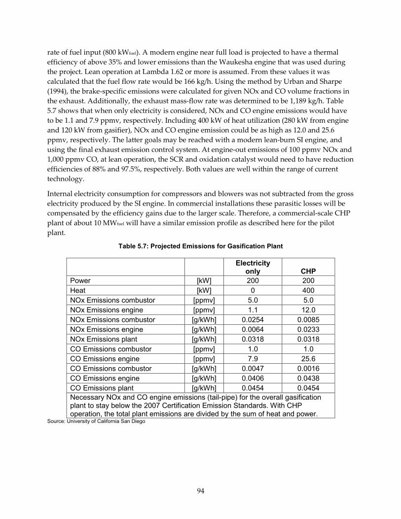
rate of fuel input (800 kWfuel). A modern engine near full load is projected to have a thermal efficiency of above 35% and lower emissions than the Waukesha engine that was used during the project. Lean operation at Lambda 1.62 or more is assumed. From these values it was calculated that the fuel flow rate would be 166 kg/h. Using the method by Urban and Sharpe (1994), the brake-specific emissions were calculated for given NOx and CO volume fractions in the exhaust. Additionally, the exhaust mass-flow rate was determined to be 1,189 kg/h. Table 5.7 shows that when only electricity is considered, NOx and CO engine emissions would have to be 1.1 and 7.9 ppmv, respectively. Including 400 kW of heat utilization (280 kW from engine and 120 kW from gasifier), NOx and CO engine emission could be as high as 12.0 and 25.6 ppmv, respectively. The latter goals may be reached with a modern lean-burn SI engine, and using the final exhaust emission control system. At engine-out emissions of 100 ppmv NOx and 1,000 ppmv CO, at lean operation, the SCR and oxidation catalyst would need to have reduction efficiencies of 88% and 97.5%, respectively. Both values are well within the range of current technology.

Internal electricity consumption for compressors and blowers was not subtracted from the gross electricity produced by the SI engine. In commercial installations these parasitic losses will be compensated by the efficiency gains due to the larger scale. Therefore, a commercial-scale CHP plant of about 10 MWfuel will have a similar emission profile as described here for the pilot plant.

Table 5.7: Projected Emissions for Gasification Plant

Electricity only CHP

Power [kW] 200 200 Heat [kW] 0 400 NOx Emissions combustor [ppmv] 5.0 5.0 NOx Emissions engine [ppmv] 1.1 12.0 NOx Emissions combustor [g/kWh] 0.0254 0.0085 NOx Emissions engine [g/kWh] 0.0064 0.0233 NOx Emissions plant [g/kWh] 0.0318 0.0318 CO Emissions combustor [ppmv] 1.0 1.0 CO Emissions engine [ppmv] 7.9 25.6 CO Emissions combustor [g/kWh] 0.0047 0.0016 CO Emissions engine [g/kWh] 0.0406 0.0438 CO Emissions plant [g/kWh] 0.0454 0.0454 Necessary NOx and CO engine emissions (tail-pipe) for the overall gasification plant to stay below the 2007 Certification Emission Standards. With CHP operation, the total plant emissions are divided by the sum of heat and power.


94

CHAPTER 5: Synthetic Bed Material and Ash Recovery Using laboratory and slip-stream systems, the performance of synthetic bed material is demonstrated. This allows the production of a recyclable ash byproduct from BCHP operations by replacing the olivine bed material used in the gasification/fluidization process with a synthetic bed material with catalytic enhancement which will not contaminate the ash and provides comparable or improved operational performance in tar reforming.

5.1 Flow Reactor Study of Synthetic Bed Material 5.1.1 Experimental Design The DFB steam gasification approach is advantageous for the synthesis of a nitrogen-free producer gas with a high heating value. The producer gas commonly includes H2, CO, CO2, H2O, CH4, C2-C5 hydrocarbons, tars, NH3 and H2S. The tar component is a mixture of aromatic hydrocarbons that are condensable at room temperatures. The tars need to be removed from the producer gas before it enters any downstream processes, as the tars can cause severe fouling and corrosion problems. Downstream (secondary step) gas-cleaning steps required for subsequent utilization are relatively expensive. The removal of tars by the use of catalyzed bed material inside the gasifier can result in reduced gas-cleaning costs.

The uncatalyzed gasifier bed materials like olivine, silica sand, and limestone display only moderate activity for tar removal. These minerals have been applied as a support for high performance metal catalyst such as nickel (Ni). Although, Ni is low cost and highly active, it undergoes severe sintering and coke deposition. Moreover, the disposal of the ash waste along with attrited gasifier bed materials from a gasification unit can also be problematic if it contains a high amount of toxic Ni. It is desired therefore, to achieve an acceptable tar removal performance of catalyzed gasifier bed materials with low Ni loading and to prevent sintering and coke desposition. In previous research the addition of Fe to Ni has been shown to prevent sintering (Baidya, 2015).

In this study a composite Ni-Fe-CaO catalyst for gasifier bed material was investigated for tar removal properties during steam reforming. The role of Fe and CaO in the promotion of the Ni loaded catalyst for higher activity and resistance to coke deposition was examined.

5.1.1.1 Experimental setup The schematic diagram of a fixed-bed reactor setup used for to evaluate catalyst performance during steam reforming for tar removal is shown in Figure 6.1. The system uses Teledyne HFC-302 mass flow controllers to feed the gases to the process manifold. The producer gas mixture is formulated with bottled gases consisting of H2, CO, CO2, CH4, and C2H4. Tar in the form of C7H8 is introduced from the liquid tank. N2 from the inert gas lines in Figure 6.1 is passed through C7H8 tank to carry vapors at room temperature to the reforming reactor. Deionized water is injected using a liquid delivery system consisting of a positive displacement pump, followed by an electric heater to vaporize the incoming liquid. A temperature recorder monitors the temperature of the vaporizer. The incoming gases are mixed in a gas-mixing chamber to ensure

95

uniform mixing before it enters the reactor. The feed and product lines are heat traced using heating tapes. A set of two three-way valves are used to bypass the reactor. The system incorporates two stages of liquid condensation, and each condenser is operated at room temperature. The non-condensable gases coming out of the condensation zone are sent to the vent lines. The composition of the outlet gases prior to condensation is analyzed online by an Agilent 3000 micro gas chromatography (GC), using four separation columns (OV-1, Plot U, Plot Q, and Molecular Sieve), and thermal conductivity detectors.

The system includes a horizontal inconel tube reactor with specifications: 2.54 cm (outer diameter) × 2.20 cm (inner diameter) × 41.91 cm (length). The catalyst bed is located at the center of the reactor, and reactor tube is heated with a split-tube tube horizontal furnace. Temperature of the furnace is maintained by a furnace controller with feedback from thermocouple in the furnace. Additional thermocouples are placed at the front, and back of the catalyst bed to record the catalyst bed temperature.

Figure 6.1: Schematic Representation of the Steam Reforming Unit with a Fixed-Bed Reactor

Typically, 2000 mg of the catalyst was weighed, and mixed with quartz chips with a ratio of 1:10 (by weight). The catalyst was reduced in situ at 800°C for 1 hour under H2 flow during the reduction step, the bed temperature was increased at 10°C per min under the inert gas flow. The reduction step is necessary to reduce oxides phases into active metallic phases. At the end of

Gas mixing chamber

Tar tank(Toluene)

Water tank

High pressure water pump Electric heater

MicroGC

Condensers

Furnace Catalyst bed

Flow controllers

Reactor bypass

Pressure transducerThermocoupleCheck valveOn/off valves3-way valveHeat trace

H2

N2

CO

CO2

CH4

O2

C2H4

Inert (N2)

Vent

Vent

96

reduction, the reactor was cooled down below 650°C under the inert gas flow. For the steam reforming experiments, the bed temperature was increased to 700°C at 10°C per min. Experiments were performed at reaction temperature of 700, 750, and 800°C, and a total flow rate of 433 standard cubic feet per minute (scfm) including H2O in gaseous state. The inlet composition molar percentage (mol %) of the producer gas mixture was: 13.4% H2, 9.8% CH4, 25.3% CO, 6.4% CO2, 40.4% H2O, 3.9% C2H4, and 0.9% C7H8. Selected feed gas composition is in accordance with the producer gas composition expected from the biomass gasification process (Anis, 2011). The C7H8 content in the simulated producer gas for the given composition is 35.7 grams per cubic nanometer (g Nm-3), which is comparable to values generally reported (Zhu, 2014) for a biomass-gasified producer gas. All the experimental data presented in this study were measured with multiple GC injections, and the averaged values are reported. Following expressions are used to determine the activity of different catalysts.

Following expressions are used to determine the activity of different catalysts.

The percent conversion for a reactant A, i.e., %, is calculated by:

( )% 100in outA A

A inA

mol molX Xmol

−=

The percent selectivity towards CO2 is based on the amount of C7H8, C2H4 and CH4 reacted:

( ) ( ) ( ) ( )2 2

int

27 8 2 4 4

% 1007 2

outCO CO

reacted reacted reactedC H C H CH

mol molCO selectivity X

mol mol mol

− =

+ +

5.1.1.2 Gasifier Bed Material Carbo HSP ceramic gasifier bed materials were acquired from CARBO Ceramics, USA. The composition (% by weight) of the bed material, as provided by supplier, includes 83.0% Al2O3, 7.0% Fe2O3, 5.0% SiO2, 3.5% TiO2, and 1.5% others. Selection of the gasifier bed material is primarily influenced by its high thermal conductivity, excellent roundness, and high-abrasion resistance; properties that are typically desired for the high-temperature biomass gasification operation in a fluidized-bed gasifier. Initially, Carbo bed materials are dried at 125°C for 24 hours to remove moisture present in the material. The dried material is referred to as a base Carbo, and is used for catalyst synthesis.

5.1.2 Laboratory Methods 5.1.2.1 Catalyst Preparation Using the Carbo gasifier bed material as a support, 1% of Ni, Fe and 1.6% (by weight) of Ni-Fe-CaO were deposited by the wet impregnation method. Ni(NO3)2.4H2O, Fe(NO3)3.9H2O and Ca(NO3)2.4H2O were used as precursors and the required amounts were dissolved in 5 ml of water to transparent solution. The solution was applied to 20 grams of Carbo support mixing with glass rod until it is homogeneously wet. The impregnated mixture was left for 12 hours and then kept at 110°C in an oven for 12 hours. The temperature of the furnace was raised by 50 degree per minute up to 800°C and calcined at this temperature for 12 hours. By heating the

97

impregnated nitrate salts, they decompose to the corresponding oxides NiO, Fe2O3 and CaO forming composites. A similar loading of CaO content in all the catalysts was maintained while various compositions with different Ni/Fe ratio from 0.0 to 1.0 were prepared. The compositions of the catalysts are referenced as follows: the composite 1.6%(Ni40Fe20Ca40)/Carbo HSP catalyst has Ni, Fe and CaO in weight proportions of 40%, 20% and 40% respectively. The loading of the active components on Carbo HSP support are mentioned in the following Table 6.1.

Table 6.1: Calculated Ni-, Fe-, and CaO-based Composite Catalyst Loading on Carbo HSP

Catalyst on Carbo HSP Catalyst Batch

Prepared(g) Loading of

Ni (g) Loading of Fe (g)

Loading of CaO (g)

1.5%Ni 20 0.32 0.0 0.0

1.6%(Ni60Ca40) 20 0.19 0.0 0.13

1.6%(Ni45Fe15Ca40) 20 0.14 0.05 0.13

1.6%(Ni40Fe20Ca40) 20 0.13 0.07 0.13

1.6%(Ni35Fe25Ca40) 20 0.11 0.08 0.13

1.6%(Ni20Fe40Ca40) 20 0.07 0.13 0.13

1.6%(Fe60Ca40) 20 0.0 0.15 0.13

1%(Ni65Fe35) 20 0.11 0.06 0.0

1%Fe 20 0.0 0.15 0.0

5.1.2.1 Characterization techniques X-ray diffraction (XRD) was performed with an X-ray diffractometer (BRUKER D2 PHASER) equipped with a monochromator for Cu Kα radiation at a DC voltage of 30 kV, and a current of 100 mA. Samples were crushed to fine powder prior to measurement. During the measurement, samples were scanned from 2θ = 20 to 60°C at the rate of 0.02°C per second. The observed patterns were identified using the International Centre for Diffraction Data (ICDD) database.

Temperature-programmed reduction (TPR) studies of the catalysts were performed to investigate the reduction behavior with a Quantachrome Instrument (ChemBET-3000 TPR/TPD). Typically, a 500 mg sample was placed in a U-shaped quartz tube, and heated from 40 to 800°C at 10°C per minute in a gas mixture containing H2 and N2. The consumption of H2 during the reduction was monitored by a thermal conductivity detector. Prior to a TPR test, the sample was outgassed under inert gas flow at 400°C for 4 hours.

The microstructures of the catalysts were characterized with a scanning electron microscope (SEM, Phillips XL30).

98

To prepare samples for transmission electron microscopy (TEM, FEI Tecnai Sphera), small amount of impregnated mixed oxides powders were separated from the Carbo HSP support and placed on the Cu grid. The samples were imaged at 200kV.

5.1.3 Results and Analysis 5.1.3.1 Catalyst Activity In the Ni-Fe-CaO mixed oxide catalyst, Fe and CaO act as promoters and therefore, it is important to determine how each plays a role in promoting Ni. The specific role of Fe and CaO in promoting Ni to achieve higher tar conversion activity was investigated. This was accomplished by stepwise addition of promoters into Ni and comparing their activities. At first, the effect of Fe addition into Ni was investigated. These samples contained no CaO. At 750°C, tar conversion activities of Ni-Fe vs pure Ni catalysts with similar Ni loading, but different Ni/Fe ratios are presented in Figure 6.2a.

The activity changes significantly different at lower (Fe/Ni = 0.125) and higher (Fe/Ni = 0.75) Fe loading into Ni. The activity increased from 49% in 1.2% Ni to 81% in 1.35% Ni-Fe sample (1.2%Ni+0.15%Fe) where a small amount of Fe was added into Ni catalyst. At higher loading of Fe into Ni (Fe/Ni = 0.75), activity was lowered from 54% in 0.6% Ni to 37% in 1.05% Ni-Fe sample (0.6%Ni + 0.45%Fe). XRD data indicated Ni-Fe alloy formation and therefore, synergistic interaction between Ni and Fe could be the basis for the enhancement at lower side relative Fe concentrations. An alternate possibility could be that at lower Fe loading, Ni was finely dispersed more due to the presence of Fe at the interface. Moreover, Fe is known to accumulate oxygen species on the surface and therefore, Ni species attached to Fe could be partially oxidized lowering the activity when Fe concentration was increased.

99

Figure 6.2: Tar Removal Efficiency in Ni vs. Ni-Fe (a) and Ni-Fe vs. Ni-Fe-CaO (b) Catalysts

(Temperature = 750°C; GHSV = 12990 cc g-1h-1)

The role of CaO was also very significant. The tar conversion efficiency of Ni-Fe is compared with Ni-Fe-CaO compositions at 750°C as presented in Figure 6.2b. There clear improvement in tar conversion activity upon addition of CaO into either Ni or Ni-Fe. As indicated in Figure 6.2b, the tar conversion increases from 44% in 1.5% Ni to 92% in 1.6% (Ni40Ca60). Similarly, tar conversion increased to 80% in 1.6% (Ni45Fe15Ca40) and to 54% in 1.6% (Ni40Fe20Ca40) from their respective counterpart without CaO, with conversions of 58% and 37%, respectively. However, at higher Fe/Ni ratios, CaO had almost no effect (at Ni/(Ni+Fe) = 0.33). At lower Fe

100

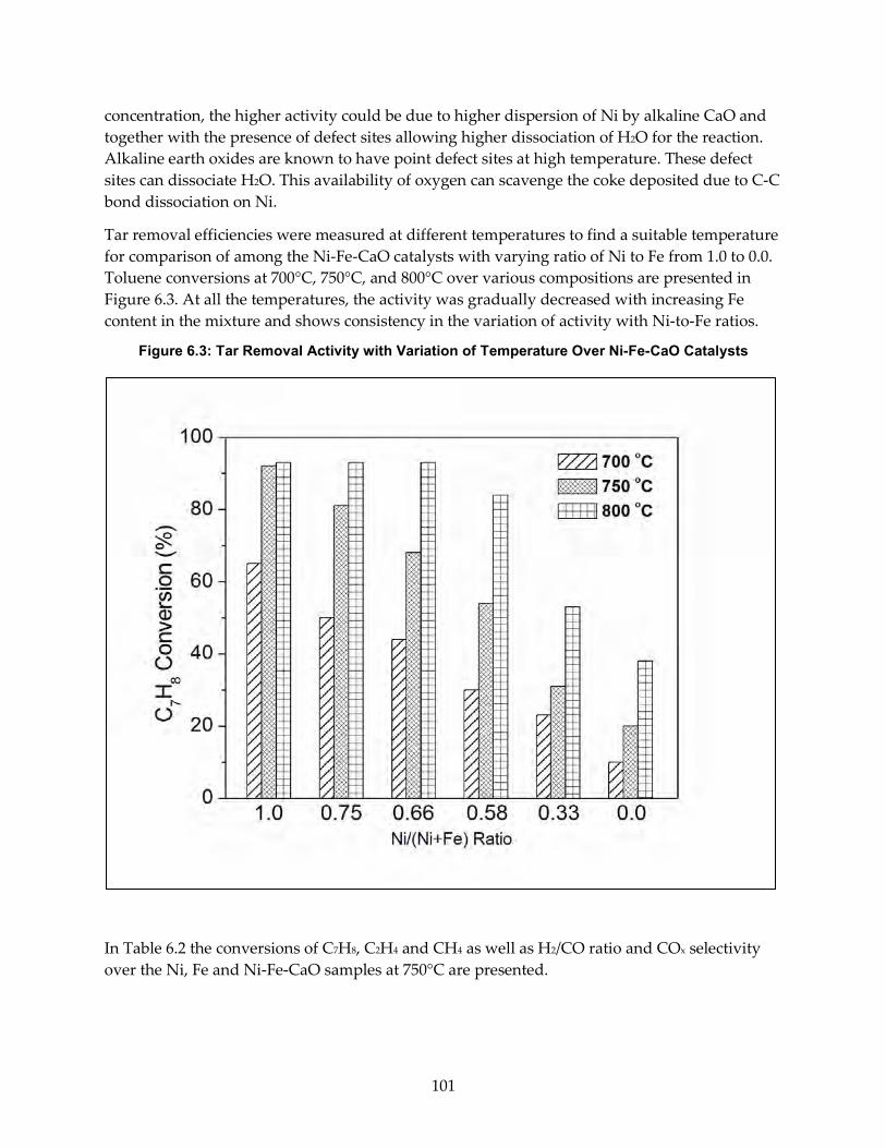
concentration, the higher activity could be due to higher dispersion of Ni by alkaline CaO and together with the presence of defect sites allowing higher dissociation of H2O for the reaction. Alkaline earth oxides are known to have point defect sites at high temperature. These defect sites can dissociate H2O. This availability of oxygen can scavenge the coke deposited due to C-C bond dissociation on Ni.

Tar removal efficiencies were measured at different temperatures to find a suitable temperature for comparison of among the Ni-Fe-CaO catalysts with varying ratio of Ni to Fe from 1.0 to 0.0. Toluene conversions at 700°C, 750°C, and 800°C over various compositions are presented in Figure 6.3. At all the temperatures, the activity was gradually decreased with increasing Fe content in the mixture and shows consistency in the variation of activity with Ni-to-Fe ratios.

Figure 6.3: Tar Removal Activity with Variation of Temperature Over Ni-Fe-CaO Catalysts

In Table 6.2 the conversions of C7H8, C2H4 and CH4 as well as H2/CO ratio and COx selectivity over the Ni, Fe and Ni-Fe-CaO samples at 750°C are presented.

101

Table 6.2: C7H8, C2H4, and CH4 Conversion Efficiency, H2 Conc., COx Selectivity, and H2/CO Ratio over Ni-Fe-CaO/Carbo Catalysts (750°C)

Catalyst on CARBO C7H8 C2H4 CH4 COx Sel

Excess H2 (%

increment) H2/CO TOF (s-1)

on Ni 1.5% Ni 44 40 3* 77 71 0.88 0.0007 1.6% (Ni60Ca40) 92 88 7 83 177 1.28 0.0019 1.6% (Ni45Fe15Ca40) 80 71 2* 96 155 1.32 0.0027

1.6% (Ni40Fe20Ca40) 68 64 2* 98 121 1.19 0.0028

1.6% (Ni35Fe25Ca40) 54 45 2* 89 116 1.20 0.0027

1.6% (Ni20Fe40Ca40) 31 28 3* 73 72 1.07 0.003

1.6% (Fe60Ca40) 20 19 4* 60 44 0.82 - 1.0% (Ni65Fe35) 40 37 2 86 91 0.92 0.0014 1.0% Fe 18 25 4* 52 32 0.72 -

* Indicates increase in CH4 concentration

Both pure Ni and Fe samples have low activity with 44 and 18% of Toluene conversion respectively. Addition of CaO along with Ni was found to be more effective showing an enhancement from 44% to 92% conversion in Ni-CaO. However, the addition of CaO along with Fe on Carbo HSP had almost no effect increasing only from 18 to 20% in Fe-CaO. A mixture of Ni and Fe with varying weight ratio in the Ni-Fe-CaO composites showed a significant trend. The 1% (Ni65Fe35) composition containing no CaO converted only 40% toluene. The toluene conversion increased significantly when CaO was further added along with Ni or Ni-Fe mixtures. The variation of Ni/Fe ratio in Ni-Fe mixture showed that as the Ni/Fe ratio was decreased, the toluene conversion activity also decreased from 80% with 1.6% (Ni45Fe15Ca40) to 31% with 1.6%(Ni20Fe40Ca40). The toluene conversion was still higher over the 1.6%(Ni35Fe25Ca40) catalyst compared to the 1.5%Ni catalyst. Similarly, C2H4 conversion also decreased systematically from 71% for 1.6%(Ni45Fe15Ca40) to 28% for 1.6%(Ni20Fe40Ca40). However, as the Fe loading was increased into the Ni-Ca catalyst, CH4 conversion changed from positive to negative value. This indicates that excess CH4 was formed in the Fe loaded sample which could be due to methane formation by breaking toluene into benzene and methane. However, the selectivity toward COx due to hydrocarbon reforming reaches an optimum value of 98% with 1.6%(Ni40Fe20Ca40). The steam reforming of tar as well as hydrocarbons adds extra H2 enriching the energy value of the producer gas. The excess H2 reached the highest increase at 155% with 1.6%(Ni45Fe15Ca40) and then decreases with increasing Fe content. Similarly, H2/CO ratio reached a maximum value of 1.32 on 1.6%(Ni45Fe15Ca40) and then decreased with decreasing Ni/Fe ratio.

The stability of the catalyst in time-on-stream was studied over selected compositions. Since 1.6% (Ni45Fe15Ca40) had higher tar conversion activity than 1.6% (Ni40Fe20Ca40) and had almost similar COX selectivity, deactivation studies was performed on both samples. The

102

toluene conversion efficiency over 1.6%(Ni45Fe15Ca40) at 800 0C for 72 hours is presented in Figure 6.4 in two segments: 48 hours on freshly reduced sample and 24 hours on regenerated sample. The catalyst activity was almost unchanged in the initial 20 hours and then slowly deactivated from the highest 99.7% to 83% at end of 48 hours. Although, deactivation of the catalyst was not severe in the initial 48 hours, the catalyst was regenerated to examine the effect on catalyst performance by the O2 /H2 sequence. The regenerated catalyst returns to almost initial activity of 98% toluene conversion and then deactivated to 80% in 24 hours time-on-stream. However, the conversion efficiency on 1.6% (Ni40Fe20Ca40) was reduced from 92% to ∼ 80% in 10 hours and remained stable at the end of 50 hours.

Figure 6.4: Time-on-Stream & Regeneration Study over 1% (Ni65Fe35), 1.6% (Ni45Fe15Ca40) and 1.6% (Ni40Fe20Ca40) Catalysts for Tar Removal from Producer Gas

Gas Hourly Space Velocity = 12,990 cc g-1h-1; Temperature = 800°C

A study on the importance of CaO on the stability of Ni-Fe-CaO was compared with 1% (Ni65Fe35) catalyst is also shown in Figure 6.4. The catalyst efficiency was lowered from 52% to 22% in just 5 hours and then starts slowly rising to 40% at the end of 48 hours. The increase could be due to accumulated carbon which also acts as catalyst. When the deactivation in

103

1.6%(Ni45Fe15Ca40) was compared with a previous catalyst performance (Baidya, 2015) of Ni-Fe/CARBO, the present catalyst has much better performance in terms of activity and resistance toward deactivation.

The turn over frequency (TOF) on the Ni atom was calculated to examine if CaO addition into Ni or Ni-Fe mixture enhances the activity of Ni (see Table 6.2). By addition of Fe or CaO into Ni, TOF increases from 0.0008 in 1.5% Ni to 0.0014 s-1 and 0.0019 s-1 in 1% (Ni65Fe35) and 1.6% (Ni60Ca40), respectively, which could be due to higher dispersion of Ni. In the presence of CaO, as Ni/Fe ratio was varied in Ni-Fe-CaO with increasing Fe content from 1.6%(Ni45Fe15Ca40) to 1.6%(Ni20Fe40Ca40), the TOF value remains in the similar range of 0.00028 s-1 on an average. This indicates that the Ni activity is positively promoted by both Fe and CaO have prominent effect.

5.1.4 Catalyst Characterizations 5.1.4.1 XRD Analysis The impregnated phases in the Ni-Fe-CaO composite catalysts were detected by XRD. As the reforming reactions were carried out on the reduced phases of the active metals, characterizations of the reduced samples were more important than the fresh oxides. In Figure 6.5 the XRD patterns of the set of Ni-Fe-CaO composites (reduced in H2 at 800°C for 1 hour) are shown. Here, the reduced Carbo HSP was used as reference to distinguish the respective peaks related to Ni, Fe, NiFe alloy or Ca oxide in the composites. The highest intensity peaks of cubic Ni(111) in NiCa/Carbo are observed at 44.6°C and 51.9°C. Similarly, cubic Fe peak was observed at 44.82° C in in FeCa/Carbo. In the presence of Fe with Ni, there is the possibility of Ni-Fe alloy formation because both are miscible since their atomic radii are similar. The highest intensity peak of NiFe alloy is located at 43.9°C. With gradually increasing Fe content into Ni, the peak intensity at 44.5°C is lowered as expected (Figure 6.5c & d) and the peak position is shifted to lower angle. In 1.6% (Ni45Fe15Ca40) (Figure 6.5c), the Ni peak is very broad and extended toward lower angle indicating a new phase. Ni(111) peak is not present in 1.6% (Ni35Fe25Ca40) (Figure 6.5d) and the indication of a new peak at slightly lower temperature is observed (marked by *). The broadening of the peak indicates high dispersion of smaller Ni particles along with Fe. However, at higher content of Fe in Ni (Figure 6.5e), the new peak belongs to neither Ni nor Fe (compared Fig 6.1.4b & f). This indicates that Ni and Fe forms a new phase, an alloy that has the highest peak at 44°. The profile of the spent catalyst of 1.6% (Ni40Fe20Ca40) (time-on-stream) is displayed in Fig Figure 6.5g, showing a distinct peak of the Ni-Fe alloy. However, the existence of Ca oxide related peaks are not observed. This may be because the CaO is not in crystalline form. As CaO is well dispersed, Ni or NiFe particles are also well dispersed on the support.

104

Figure 6.5: XRD Patterns of (a) 1%Ca, (b) 1.6%(Ni60Ca40), (c) 1.6%(Ni45Fe15Ca40), (d) 1.6%(Ni35Fe25Ca40), (e) 1.6%(Ni20Fe40Ca40), (f) 1%(Fe60Ca40) and (g) Spent Catalyst of

1.6%(Ni40Fe20Ca40)

* indicates Ni-Fe alloy peak.

5.1.4.2 TPR Analysis Figure 6.6 presents the temperature programmed reduction (TPR) profiles of pure Carbo HSP support, Ni-CaO, Fe-CaO and Ni-Fe-CaO mixed oxides impregnated Carbo HSP samples. As expected, reduction in the Carbo HSP starts occurring at high temperature above 500 0C (Figure 6.6a). However, the major reduction of Ni, Fe oxides occur below 550 0C. The temperature of reduction profiles of the impregnated oxides provides us information about the interaction among these metals. As a reference, TPR of NiO is also presented (dotted profile) for quantitative analysis. The peak position at 345 0C was corroborated in the literature [4]. The peak area corresponds to 170 µmol H2. Therefore, the amount of reduction in Carbo HSP corresponds to 51 µmol H2/gcat, whereas total reduction in Ni-Fe-CaO impregnated oxides

105

remained ∼ 210 µmol H2/gcat.The comparatively small peak arising at ∼ 340°C is due to reduction of NiO species in the Ni-CaO or Ni-Fe-CaO mixed oxides (Figure 6.6b – e). The reduction peak of Fe oxides in Fe-CaO occurs at 520°C (Figure 6.6f). A new peak arising at ∼ 420°C with growing intensity as Ni/Fe ratio decreases, while peak intensity of Ni oxide reduction at ∼ 345°C decreases. Thus, the reduction profile of 1.6% (Ni20Fe40Ca40) has neither features of Ni oxide nor Fe oxides reduction (Figure 6.6e). This is an indication of synergistic interaction between Ni and Fe, in which, Fe is reduced at a lower temperature in presence of Ni. The can be explained as follows. As Ni metal is formed at lower temperature, Fe oxide will see dissociated hydrogen from the Ni surface by a spill over process leading to the reduction of Fe oxide at lower temperature. However, the nature of the Ni-CaO and Ni-Fe profiles are not too different (Figure 6.6b & g).

Figure 6.6: TPR Profiles of (a) Carbo HSP, (b) 1.6%(Ni60Ca40), (c) 1.6%(Ni45Fe15Ca40), (d) 1.6%(Ni35Fe25Ca40), (e) 1.6%(Ni20Fe40Ca40), (f) 1%(Fe60Ca40) and (g) 1%(Ni50Fe50)

5.1.4.3 SEM Analysis In Figure 6.7 SEM images are presented of the 1.6% (Ni40Fe20Ca40) and 1% (Ni65Fe35) catalysts as freshly reduced (Figure 6.7a and d, respectively) as well as spent catalysts (Figure 6.7b, c and Figure 6.7e, f) with 15,000 and 5,000 magnifications respectively in time on stream for 50 hours. The beneficial effect of CaO comes from the high dispersion of Ni-Fe as observed

106

from the homogeneous distribution of particles in the Figure 6.7a. A fine porous dispersion of the mixture of Ni, Fe and CaO is observed in the freshly reduced 1.6% (Ni40Fe20Ca40) sample (Figure 6.7a) and it is difficult to distinguish Ni, Fe or CaO in the composite. However, larger particles of Ni and Fe metals are visible in the freshly reduced samples. The spent catalysts have marked difference in their resistivity toward particle agglomeration at high temperature as well as Carbon deposition on the active sites. Neither large particle formation nor carbon deposition was observed in the spent catalyst of 1.6% (Ni40Fe20Ca40). On the other hand, Ca free sample suffers from agglomeration of Ni, Fe particles formation. Filament like deposited Carbon species are observed in this sample, as marked by circles (Figure 6.7e and f). Therefore, Ca has a beneficial effect in keeping Ni and Fe components in well dispersed forms under extreme conditions.

Figure 6.7: SEM Images of Freshly Reduced and Spent Catalysts of 1.6% (Ni45Fe15Ca40) (a,b), 1.6% (Ni40Fe20Ca40) (c,d) and 1% (Ni65Fe35) (e,f), Respectively

5.1.4.4 TEM Analysis The TEM images of 1.6% (Ni45Fe15Ca40), 1.6% (Ni40Fe20Ca40) and 1% (Ni65Fe35) catalysts as freshly reduced as well as spent in Time-on-Stream are presented in Figure 6.7. In the freshly reduced 1.6% (Ni45Fe15Ca40) sample, the presence of lattice fringes on cubic particles indicates a well-defined crystalline form (Figure 6.8a). The particles have an average size of 15 nm dispersed uniformly on the surface, but it is not clear whether these belong to Ni, Fe or Ni-Fe alloy. After regeneration treatment with an O2/H2 sequence on this sample, the particles size distribution became larger than 200 nm (Figure 6.8b). In 1.6% (Ni40Fe20Ca40), no lattice fringe was observed in the freshly reduced sample because electron beam cannot transmit through the larger particles ranging from less than 100 nm to more than 200 nm (Figure 6.8c). After 48 hours of time on stream, there is no visible change in the particle size distribution (Figure 6.8d) unlike

107

in the above sample. The catalyst without CaO (1% (Ni65Fe35)) led to formation of much larger particles after being in stream for 48 hours (Figure 6.8e & f).

Figure 6.8: TEM Images of Freshly Reduced (a, d) and Spent Catalysts of 1.6%(Ni40Fe20Ca40) (b, c) and 1%(Ni65Fe35) (e, f) Respectively

5.1.5 Conclusions A new Ni-Fe-CaO composite catalyst for increasing the tar reforming activity of gasifier bed material with the different compositions was prepared by wet impregnation method. XRD shows Ni-Fe alloy formation in the Ni-Fe-CaO catalysts and their synergistic interaction (indicated in TPR) leads to increase in TOF on Ni atoms. CaO provided the enhanced activity and stability toward catalyst deactivation on the catalyst by maintaining the dispersion on the support. The tar removal performance of the Ni-Fe-CaO catalysts was much superior compared

108

to Ni-Fe catalysts. Both 1.6%(Ni45Fe15Ca40) and 1.6%(Ni40Fe20Ca40) showed optimum activity toward C7H8 conversion as well as the highest COx selectivity. The 1.6% (Ni40Fe20Ca40) catalyst showed optimum activity toward C7H8 conversion as well as highest COx selectivity. The 1.6% (Ni45Fe15Ca40) catalyst demonstrated very slow deactivation with a decrease in conversion efficiency from 99.7% to 83% for the first 48 hours and the conversion efficiency reduced from 98% to 80% after regeneration with Oxygen/Hydrogen treatment. The spent sample in the stream for a long time show large particle formation. Coke deposition in the catalyst bed did not affect the catalyst activity. This Ni-Fe-CaO catalyst is a promising candidate for application to gasifier bed material.

5.2 Fixed Bed Reactor Study of Synthetic Bed Material A portable fixed-bed tar reformer was developed to test tar reforming on an existing gasifier. The tar reformer is able to be filled with various catalysts and evaluate different operating temperatures and residence times.

5.2.1 Experimental Design At core of the design is a three-zone tube furnace that allows a catalyst to be heated up to 900°C. Flow controllers and pumps are available to move the required gases through the catalyst bed. The gases include laboratory gases for calibration, activation, regeneration, or producer gas from a gasifier. Figure 6.9 shows a schematic of the experimental setup.

109

Figure 6.9: Schematic of Portable Tar Reformer


Tar sampling port 1

Tar sampling port 2

Flow controllers

To scrubber or oxidizing unit

To Gas analyzer

Slip stream to GC

Gas supply lines

HPLC pump (water)

Evaporator

From gasifier

Furnace

N2 or He

H2

Air or other

Thermocouple 6

Thermocouple 7

P

Pressure relief valve

Pump

Synthetic tars, steam, helium

Catalyst

Hot filter Impinger with biodiesel

Hot filter Impinger with biodiesel

Pump

Pump

Sample from hot filter with FTIR, GC

HPLC pump (tars)

Thermocouple 8

Ice trap

Scale for condensate

Sampling line before catalyst

Sampling line after catalyst

110

Figure 6.10: Photograph of Fixed-Bed Tar Reformer

Photo Credit: University of California San Diego

5.2.2 Laboratory Methods The difference between the portable fixed-bed reformer and the laboratory fixed-bed reactor is that the portable reformer is built for slightly higher flow rates such as a typical slip stream

111

from an actual gasifier (i.e., a few liters per minute). To accommodate the higher flow rates, catalyst loading and heating power of the tube furnace are higher. A slip stream from a gasifier may contain insufficient amounts of water necessary for the reforming reaction. For this reason, the capability exists to blend the stream from the gasifier with a stream containing steam. In order to quantify the flow rates of each stream, the steam is blended with helium as tracer gas.

To conduct experiments when the gasifier is not operating, a test-gas generator is part of the experimental setup. This test-gas generator allows the operator to blend gases (hydrogen, nitrogen, helium) with steam and tars and requires two high-performance liquid chromatography pumps to control the correct flow rate of water and tars, respectively, to an evaporator. Both water and tar flow rates are additionally metered by scales. The tar mixture can contain larger tar compounds as long as they are soluble in benzene and toluene, which are used as tar-like solvents. Table 6.3(b) shows an example of a mixture of nitrogen, steam, and 41g/Nm3 of tars. The tars in turn are a mixture of 61w% benzene, 29.3w% toluene, 7.4w% naphthalene, and 1.8% acenaphthylene.

Table 6.3: Overview of Target Test Composition

(a) Composition of target tar mixture. (b) Composition of target gas composition Source: University of California San Diego

Typical operating conditions are 800°C for the catalyst bed and a total flow rate of 4 slpm (referenced to 0 °C and 1 atm). Under these conditions, the space time - the time the gas would reside in the empty catalyst volume - is approximately 0.23 seconds. A catalyst amount in the range of 10-30 g is typical for the 1-inch reactor tube (0.875-inch inside diameter [ID]). The remainder of the volume is filled with quartz chips. The quartz chips ensure that heat can be transferred from the tube walls to the catalyst to compensate for the energy used in the endothermic reaction.

Using nickel-based catalysts requires the catalyst to be activated (i.e., the conversion of nickel oxide to nickel). This is performed under a reducing atmosphere of 5% hydrogen in nitrogen at 800 °C and a flow rate of 2 standard liters per minute (slpm) for one hour. If the catalyst was deactivated by carbon deposition, a regeneration step was included before the activation. This step used a composition of 2% oxygen in nitrogen, a total flow rate of 3 slpm and a temperature of 600 °C.

Compound Mole fraction Mass fractionBenzene 67.1% 61.5%Toluene 27.0% 29.3%Naphthalene 4.9% 7.4%Acenaphthylene 1.0% 1.8%

Synthetic tar mixtureCompound Mole fraction Mass fractionN2 58.9% 67.0%H2O 40.0% 29.2%Tars (41 g/Nm3) 1.1% 3.7%

Flow composition

(a) (b)

112

5.2.3 Results and Analysis Several experiments were conducted on synthetic tars (from chemicals) and real tars (from a gasifier). One issue that is prevalent with nickel catalysts is the formation of coke. Tar reforming reactions require hydrogen atoms, either in the form of large concentrations of hydrogen gas or steam. It the tar concentrations are high and the producer gas has been cooled down, there is usually an insufficient amount of steam available to prevent coke formation and the catalyst can deactivate within a very short time. Figure 6.11(a) shows the position of the catalyst relative to the three zones of the furnace. Figure 6.11(b) shows a catalyst that was deactivated by coke formation. The coke formation started to block the top surface of the catalyst, reducing the available catalyst surface area and the conversion efficiency over time. This phenomenon happened during the first test on producer gas from the gasifier. The catalyst started noticeable deactivation within minutes.

To investigate the deactivation, several tests were conducted on different tar mixtures and operating conditions. The tests were conducted in the following manner. When starting the experiment, the initial conversion factor was recorded by relating the tars at the inlet to the tars at the outlet of the reactor. This conversion factor depends on temperature, gas composition, and - most importantly - on the gas flow rate and amount of catalyst. During the subsequent experiment, the conversion factor is observed as a function of time. A measure of deactivation, called relative activity, is defined by comparing the conversion factor to the initial conversion factor:

==

=

=

0,,

,

,

,

0 log

log_Re

toutlettars

inlettars

outlettars

inlettars

t

yy

yy

ActivityActivityActivitylative

The expression called activity accounts for the exponential decay of the tar concentration in a first-order reaction. For example, if the conversion of tars changes from a factor 100 to a factor 10, then the activity of the catalyst has dropped in half (log(10)/log(100)=1/2). This is equivalent to half of the catalyst being active and allowing a tar conversion of a factor of 10, while the other half of the catalyst being blocked by coke and not allowing an additional factor 10 (for a total factor of 100).

Since benzene and toluene are the only tars readily measured by gas chromatograph and FTIR, they are used to characterize the deactivation. In the above equation, ytar denotes the mass fraction of benzene and toluene in the gas mixture. The subscript t=0 refers to the time of the start of the reforming experiment.

Figure 6.12 shows that the deactivation of the catalyst depends on the type of tar. Starting with the mixture of tars given in Table 6.3(a), some tars were selectively removed to obtain different combinations, including pure toluene. For experiments that include naphthalene, a drop in relative activity is observed much sooner than for mixtures including benzene, toluene, or

113

acenaphthylene. Coke formation is therefore a significant problem in the presence of naphthalene, one of the major tars.

Figure 6.13 shows that deactivation due to coke formation can be reduced when less catalyst is used in a given volume. Even though the conversion efficiency for benzene and toluene starts out at a lower rate (75% versus 96%), it does not drop as much over time as for the dense packing. Both experiments included naphtahlene in the feed. Due to the endothermic reactions of tar reforming, the temperature can drop locally which accelerates the coke formation. Figure 6.14 confirms that the temperature has a strong effect on coke formation, with 825°C almost preventing any catalyst deactivation. For a given flow rate and tar loading, sufficient steam, hydrogen, and temperature are necessary for operating a nickel-based catalyst over extended periods of time.

Figure 6.11: Catalyst in Reactor Tube (a) and After Removal (b)

Source and Photo Credit: University of California San Diego

Catalyst and quartz chips

Quartz chips

Quartz wool

Flow direction

After removal of deactivated catalyst

Three-zone furnace

Inconel tube (1” OD)

(a) (b)

114

Figure 6.12: Deactivation of Nickel Catalyst Depending on Tar Type

Deactivation of nickel catalyst as a function of time and tar type by comparing the conversion of benzene and toluene with their initial conversion. The temperature is 800 C, the flow rate is 4 slpm, the catalyst loading is 25 g, the tar loading is 41 g/Nm3, and the mole fraction of steam is 35% with a balance of nitrogen. Source: University of California San Diego

Figure 6.13: Deactivation of Nickel Catalyst Depending on Catalyst Loading

Deactivation of nickel catalyst as a function of time and catalyst loading by comparing the conversion of benzene and toluene with their initial conversion. The loose pack contains 13 g of catalyst in 85 g of quartz chips. The dense pack contains 25 g of catalyst in 57 g of quartz chips. The temperature is 800 C, the tar loading (benzene, toluene, naphthalene) is 41 g/Nm3, the flow rate is 5 slpm, the mole fraction of steam is 30% and that of hydrogen is 40%, the balance is nitrogen or helium. Source: University of California San Diego

115

Figure 6.14: Deactivation of Nickel Catalyst Depending on Temperature

Deactivation of nickel catalyst as a function of time and temperature by comparing the conversion of benzene and toluene with their initial conversion. The catalyst loading is 13 g, the flow rate is 5 slpm, the tar loading (benzene, toluene, naphthalene) is 41 g/Nm3, the mole fraction of steam is 30% and that of hydrogen is 20%, with a balance of nitrogen. Source: University of California San Diego

The producer gas from the gasifier is cleaned by a particulate filter and scrubber. This removes most of the water from the gas and leaves a moisture level corresponding to the vapor pressure at the scrubber outlet temperature. At a temperature of 38 °C, the mole fraction of water in the gas is approximately 7%. To add additional water to the inlet stream for the catalyst, the producer gas stream was blended with an additional stream containing a mole fraction of 31% of steam in helium. The flow rate of this stream was measured as 1.93 slpm (referenced to 0 °C, 1 atmosphere). Helium was later used to determine the flow rate of the slip stream of producer gas to the tar reformer. During Test 4, the tar reformer was operated on producer gas from 1:56pm until 4:15pm (Figure 6.15). The producer gas slip stream was determined to be 1.72 slpm during this time. The total flow rate of gas into the flow reactor was therefore 3.65 slpm, similar to the flow rates in the preliminary tests. The catalyst was loosely packed (13 g) together with quartz chips (85 g).

Table 6.4 shows the measured composition of the outlet stream. It also shows the computed dry gas composition after the ice bath, with an estimated mole fraction of water of 1%. The dry gas flow rate was verified using a wet test meter. The wet gas flow rate after the tar reformer was then calculated as 3.7 slpm. This is consistent with the reformer inlet flow rate of 3.65 slpm, since during the reforming reactions, the number of moles increase. Besides benzene and toluene, larger tars are also present in the producer gas. Those tars were not measured with the micro gas chromatograph and would need other instruments. During the reforming of larger tars, some smaller aromatic molecules such as benzene and toluene are formed. Consequently,

116

the exact conversion efficiency was not quantified during the reforming of producer gas. The conversion depends strongly on the amount of catalyst and can be selected based on the desired cost/conversion trade-off. A more important factor in this test was to determine any operational difficulties or catalyst deactivation.

During the 2.3-hour operation on producer gas, no deactivation of the catalyst was found. This was verified by testing the catalyst after the producer-gas test using 41 g/Nm3 of toluene, 30% steam with helium as the balance. At a flow rate of 4 slpm and a temperature of 800 C, a conversion efficiency of 80% was measured, which was the baseline conversion efficiency established for toluene at these conditions and catalyst loading.

Deactivation by sulfur is another aspect that needs to be considered for using nickel-based catalysts on real producer gas. For that, longer-term studies and additional measuring instruments are necessary.

Figure 6.15: Operation of Tar Reformer on Producer Gas


0

0.2

0.4

0.6

0.8

1

1.2

1.4

1.6

1.8

2

0

100

200

300

400

500

600

700

800

1:40 PM 2:00 PM 2:20 PM 2:40 PM 3:00 PM 3:20 PM 3:40 PM 4:00 PM 4:20 PM

Flow

Rat

es o

f Wat

er a

nd H

eliu

m

Tem

pera

ture

[C]

Time

Inlet Temperature, T4 [C]

Outlet Temperature, T6 [C]

Water addition [g/min]

Helium flow rate [slpm]

117

Table 6.4: Tar Reformer Outlet Composition

Parameter Units Wet Gas Dry Gas Flow rate [slpm] 3.7 3.1 H2 [mole%] 0.187 0.221 CO [mole%] 0.138 0.163 CO2 [mole%] 0.078 0.092 CH4 [mole%] 0.037 0.043 C2H4 [mole%] 0.006 0.007 C6H6 [mole%] 0.000800 0.000956 C7H8 [mole%] 0.000032 0.000038 H2O [mole%] 0.162 0.010 He [mole%] 0.356 0.420 N2 [mole%] 0.036 0.042 Tar reformer outlet gas composition. The wet gas composition was measured by gas chromatograph. The flow rate of the dried gas was measured with a wet test meter. Numbers in italic were computed from the measured numbers.


5.3 Laboratory Gasifier Reactor Study of Synthetic Bed Material 5.3.1 Experimental Design With the goal of running the laboratory gasifier on CarboHSP synthetic bed material, a fluidization study was developed to investigate the laboratory reactor ability to operate with the new bed material. This work was performed in conjunction with the previously reported “Increasing Renewable Energy by Almond Shell Gasification” experiments (Cattolica, 2014).

An investigation into the fluidization properties of CarboHSP (Carbo Ceramics; Houston, Texas) was compared with Investocast 60 (NARCO; Pleasanton, California). Material properties of the two bed materials are shown in Table 6.5. Heat capacity for aluminum oxide (Al2O3), silicon dioxide (SiO2), Titanium dioxide (TiO2), and iron oxide (Fe2O3) were calculated by the Shomate Equation using data obtained by Chase (1998) for the temperature range 298 – 847 °K. The coefficients are shown in Table 6.6. The CarboHSP bed material has higher aluminum oxide and iron oxide content, but lower silicone dioxide content than the Investocast 60. Heat capacity of the two materials is nearly identical. The difference in elemental composition may affect catalytic activity within the gasifier, resulting in a change in gas or tar composition. Mean diameter of the CarboHSP is 95% larger than the Investocast material, and apparent specific gravity is about 30% higher, resulting in the CarboHSP fluidized bed being filled with larger, denser particles.

118

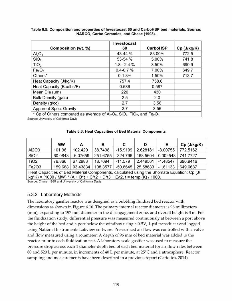
Table 6.5: Composition and properties of Investocast 60 and CarboHSP bed materials. Source: NARCO, Carbo Ceramics, and Chase (1998).

Composition (wt. %) Investocast

60 CarboHSP Cp (J/kg/K) Al2O3 43-44 % 83.00% 772.5 SiO2 53-54 % 5.00% 741.8 TiO2 1.8 - 2.4 % 3.50% 690.9 Fe2O3 0.4-0.7 % 7.00% 649.7 Others* 0-1.8% 1.50% 713.7 Heat Capacity (J/kg/K) 757.4 758.6 Heat Capacity (Btu/lbs/F) 0.586 0.587 Mean Dia (µm) 220 430 Bulk Density (g/cc) 2.5 2.0 Density (g/cc) 2.7 3.56 Apparent Spec. Gravity 2.7 3.56 * Cp of Others computed as average of Al2O3, SiO2, TiO2, and Fe2O3


Table 6.6: Heat Capacities of Bed Material Components

MW A B C D E Cp (J/kg/K)

Al2O3 101.96 102.429 38.7498 -15.9109 2.628181 -3.00755 772.5162 SiO2 60.0843 -6.07659 251.6755 -324.796 168.5604 0.002548 741.7727 TiO2 79.866 67.2983 18.7094 -11.579 2.449561 -1.48547 690.9416 Fe2O3 159.688 93.43834 108.3577 -50.8645 25.58683 -1.61133 649.6687 Heat Capacities of Bed Material Components, calculated using the Shomate Equation: Cp (J/ kg*K) = (1000 / MW) * (A + B*t + C*t2 + D*t3 + E/t2, t = temp (K) / 1000.

Source: Chase, 1998 and University of California Davis

5.3.2 Laboratory Methods The laboratory gasifier reactor was designed as a bubbling fluidized bed reactor with dimensions as shown in Figure 6.16. The primary internal reactor diameter is 96 millimeters (mm), expanding to 197 mm diameter in the disengagement zone, and overall height is 3 m. For the fluidization study, differential pressure was measured continuously at between a port above the height of the bed and a port below the windbox using a 0-5V, 1-psi transducer and logged using National Instruments Labview software. Pressurized air flow was controlled with a valve and flow measured using a rotameter. A depth of 96 mm of bed material was added to the reactor prior to each fluidization test. A laboratory scale gasifier was used to measure the pressure drop across each 1 diameter depth bed of each bed material for air flow rates between 80 and 520 L per minute, in increments of 40 L per minute, at 25°C and 1 atmosphere. Reactor sampling and measurements have been described in a previous report (Cattolica, 2014).

119

Figure 6.16: Schematic of the Fluidized Bed Gasifier


5.3.3 Results and Analysis Results of the pressure drop tests are shown in Figure 6.17 and Figure 6.18, and a summary of the results are given in Table 6.7.

120

Figure 6.17: Bed Pressure of the CarboHSP Material (left), and 20-pt Average of the Bed Pressure (right)


Figure 6.18: Bed pressure of the NARCO Investocast 60 bed material (left), and 20-pt average of the bed pressure (right)


121

Table 6.7: Bed Pressures for Investocast and Carbohsp Bed Materials

Investocast CarboHSP

flow (lpm)

Bed pressure (psi) Bed pressure (psi) Average Stdev Max Average Stdev Max % diff.

80 0.062 0.081 0.202 0.231 0.058 0.372 271 120 0.160 0.030 0.214 0.226 0.022 0.272 42 160 0.175 0.048 0.300 0.234 0.044 0.322 33 200 0.194 0.036 0.250 0.248 0.036 0.356 28 240 0.193 0.056 0.328 0.232 0.049 0.33 20 280 0.200 0.069 0.328 0.261 0.077 0.41 30 320 0.203 0.118 0.416 0.275 0.094 0.458 36 360 0.212 0.100 0.390 0.318 0.130 0.576 50 400 0.181 0.067 0.346 0.280 0.101 0.608 55

Average, standard deviation, and maximum bed pressure for Investocast and CarboHSP bed materials. Percent increase in average bed pressure observed using CarboHSP as compared to Investocast is shown in the far right column.


Results show that the CarboHSP bed exhibited higher pressure drop than the Investocast bed. At 360 L per minute, average pressure drop across the CarboHSP was 0.318 psi (2190 Pascals [Pa]) and peak pressure reached 0.576 (4000 Pa), which is 50% higher than average pressure drop due of Investocast at the same flow rate. Maximum pressure drop of the CarboHSP was a spike observed at 480 L per minute that reached 0.734 psi (5060 Pa).

122

CHAPTER 6 Technical and Economic Analysis for BCHP Commercialization Techno/economic models for the evaluation of the commercialization of BCHP were developed to analyze commercial systems. The models include: a thermochemical process design model for the BCHP process at demonstration and commercial scale, a carbon and material life cycle analysis for the BCHP process at commercial scale, and a pro forma economic model of a commercial scale BCHP plant based on the almond byproduct biomass resource.

6.1 BCHP Process Model A thermochemical process demonstration scale design model was developed for the BCHP technology to evaluate system designs at commercial scale.

6.1.1 Model Basis The BCHP gasification reactor was modeled using Aspen Plus chemical process simulator version 8.6. A detailed description of the pilot plant can be found in earlier sections of this report. Figure 7.1 shows a screenshot of the flow diagram in Aspen’s user interface.

Figure 7.1: Screenshot of the Flow Diagram in Aspen’s User Interface


The pilot plant was built on-site at the Woodland Biomass Research Center (WBRC) in Woodland, California. Figure 7.2 shows a rendering of the actual reactor with streams labeled similar to the Aspen flowsheet above for ease of reference.

123

Figure 7.2: Rendering of the Reactor with Streams Labeled Similar to the Aspen Flowsheet


124

6.1.2 Model Description The gasifier section of the Aspen model comprises several process steps in order to simulate the single gasifier vessel depicted in Figure 7.1. Figure 7.3 shows the process steps in the gasifier, as well as the process streams into and out of the gasifier. The main inputs into the gasifier are the biomass feed (wet, stream: BIOMASS), the superheated steam (to the bottom of the gasifier, stream: STEAM-G), the heated bed material from the combustor cyclone (stream: CYCL-REC), and nitrogen from various purge flows (for feeding system and sensors, stream: NITROGEN). The main outputs are the product gas and the mixture of bed material and char (flowing to the combustor, stream: COMB-IN). The gasification is modeled using the following process steps. Biomass is decomposed into moisture and the chemical elements according to the ultimate analysis of the biomass (process: PYROL of type RYIELD). The element carbon is split in a separator (process: SEP) according to the proximate analysis of the biomass. This determines how much char (the fixed carbon, stream: CHAR) is mixed with the bed material from the gasifier (streams: GASI-OUT=BED-MAT) in a mixer (process: MIX). The remainder of the carbon as well as the other elements enter the gasifier (process: GASIFIER of type RGIBBS), where they form selected output gas components according to restricted equilibrium. The restricted equilibrium is necessary because the producer gas (stream: PROD-GAS) is not in equilibrium, indicated by larger amounts of CH4 and CO. Two reactions were chosen in the restricted-equilibrium approach. By specifying the reaction rate of the water-gas shift reaction, the amount of CO can be matched with the measured CO concentration in the producer gas. By specifying the reaction rate of a theoretical formation of CH4 from the elements (C+4H), the amount of CH4 can be matched with the measured value. The selected values were 1.1 kmol/hr for both reactions.

Figure 7.3: Process Boundaries for the Gasifier Vessel

Process Boundaries for the Gasifier Vessel. The streams crossing the dashed boundary represent inputs to or outputs from the gasifier vessel. Source: University of California San Diego

Table 7.1 lists the components that were defined in the simulation of the biomass pilot plant. The components are then available for the various process steps and streams. Not all components need to be selected. For example, the component Carbon can be selected to

125

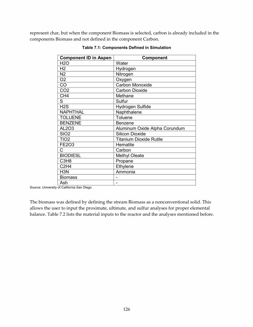
represent char, but when the component Biomass is selected, carbon is already included in the components Biomass and not defined in the component Carbon.

Table 7.1: Components Defined in Simulation

Component ID in Aspen Component H2O Water H2 Hydrogen N2 Nitrogen O2 Oxygen CO Carbon Monoxide CO2 Carbon Dioxide CH4 Methane S Sulfur H2S Hydrogen Sulfide NAPHTHAL Naphthalene TOLUENE Toluene BENZENE Benzene AL2O3 Aluminum Oxide Alpha Corundum SIO2 Silicon Dioxide TIO2 Titanium Dioxide Rutile FE2O3 Hematite C Carbon BIODIESL Methyl Oleate C3H8 Propane C2H4 Ethylene H3N Ammonia Biomass - Ash -


The biomass was defined by defining the stream Biomass as a nonconventional solid. This allows the user to input the proximate, ultimate, and sulfur analyses for proper elemental balance. Table 7.2 lists the material inputs to the reactor and the analyses mentioned before.

126

Table 7.2: Material Input to the Reactor

Biomass Feed Rate [kg/hr] 182

Proximate Analysis (wet basis)

Element Value Moisture 9.4% Fixed Carbon 19.3% Volatile Material 69.3% Ash 2.0%

Ultimate Analysis (dry basis) Element Value

Ash 2.2% Carbon 50% Hydrogen 5.8% Nitrogen 0.47% Chlorine 0 Sulfur 0.03% Oxygen 41.5%


Table 7.3 lists the additional flow rates to the plant (besides biomass). The steam enters the reactor in two separate locations. The first is at the bottom of the gasifier and the second is at the upper loop seal below the cyclone. The bed material is added to the combustor and then circulates back to the cyclone, gasifier, and finally back to the combustor, all at the same mass flow rate. Air enters the combustor in three main locations plus an additional amount used in the auxiliary burner. Air was defined as having a 0.79 and 0.21 mole fraction of nitrogen and oxygen, respectively. The composition of the bed material is shown in Table 7.4.

Table 7.3: Process Flow Rates for the Model

Input Location Value per Second Value per Hour Steam Into Gasifier 0.0192 kg/s 69.1 kg/hr Steam Into Upper Loop Seal 0.0066 kg/s 23.8 kg/hr Air Into Combustor (1st+2nd+3rd Stage) 0.213 kg/s 766.8 kg/hr Air Into Auxiliary Burner 0.05 kg/s 180 kg/hr Propane Into Auxiliary Burner 0.0037 kg/s 13.3 kg/hr Nitrogen Into Gasifier 0.0045 kg/s 16.2 kg/hr Bed Material Circulation Rate 2.53 kg/s 9108 kg/hr


127

Table 7.4: Bed Material Composition

Input Total Value AL2O3 0.82 SIO2 0.07 TIO2 0.04 FE2O3 0.07


6.1.3 Model Performance Table 7.5 shows the mass-flow rates of the calculated streams from the Aspen model. The stream labels are consistent with the process-flow diagram in Figure 7.1. Table 7.6 shows the composition of selected gaseous streams. The measured producer-gas composition is shown for comparison. It agrees reasonably well with the computed values. This indicates a good closure of the material balances for the pilot plant as well as good performance of the restricted equilibrium model. The result for the computed heat loss from the gasification system is 141 kW. This includes the gasifier, combustor, cyclone, and upper loop seal. It does not include the heat in the hot gaseous stream. The heat from those streams is recovered using heat exchangers. It is used for generating and superheating the steam and for preheating the combustor air. There is generally some excess heat available that can be used for CHP. This amount was not calculated from the Aspen model because the heat recovery system and its associated heat losses were not included in the model.

Table 7.5: Computed Mass-Flow Rates from the Model

Stream Mass-Flow Rate

[kg/s] Mass-Flow Rate

[kg/hr] CHAR 0.0098 35 COMB-IN 2.54 9143 CYC-FEED 2.81 10103 CYCL-REC 2.53 9124 DEC-CHAR 0.0506 182 DECOMP 0.0408 147 FLUEGAS 0.279 1003 GASI-OUT 2.53 9112 H2O-SCRB 0.0148 53 PG-DRY 0.0531 191 PROD-GAS 0.0678 244


128

Table 7.6: Gas Composition in Mole Fractions

Component FLUEGAS PROD-GAS PG-DRY Producer Gas (meas.) H2O 0.073 0.280 0.072 0.070 H2 0.0 0.277 0.356 0.335 N2 0.746 0.046 0.059 0.063 O2 0.108 0.0 0.0 0.0 CO 0.0 0.220 0.283 0.263 CO2 0.073 0.094 0.121 0.161

CH4+HC 0.0 0.083 0.108 0.106 H2S 0.0 0.00012 0.00015 0.00030

Gas composition of flue gas (stream: FLUEGAS, combustor outlet), producer gas (stream: PROD-GAS, gasifier outlet), and dried producer gas (stream: PG-DRY, scrubber outlet). Values are in Mole fractions. The last column shows the measured dried gas composition for comparison. Source: University of California San Diego

6.1.4 Evaluation of Commercial Scale BCHP Systems The process model was extended to simulate a commercial-scale sized BCHP plant that was projected to have an electrical output power of 10 times larger than that of the pilot plant (2.5 MWe compared to 250 kWe). In this model, the producer gas rate, the biomass rate, the bed-material circulation rate, and most other flow rates were projected to be 10 times larger as well. The one main difference was in the flow to the combustor vessel of the commercial plant. Since a 10-times larger plant has a surface/volume ratio of about 2.15 times smaller (10(1/3)) than that of the pilot plant, heat losses are also estimated to be 2.15 times smaller relative to the power input. This reduces the amount of co-firing of any additional propane in the combustor, which in turn reduces the amount of air needed in the combustor significantly. To provide some additional heating besides the char from the gasifier, the char collected in the producer gas filter, as well as the tars and biodiesel from the scrubber, can now be used in the combustor. In the Aspen model, this is modeled as an injection of the biodiesel, at a rate necessary to represent all three components. Other benefits arise from the larger plant. For example, a higher circulation rate of bed material can be achieved relative to the biomass feed, resulting in smaller temperature differences between combustor and gasifier. Also, less inert gas is needed for purging the feeding system and sensors, increasing the product-gas quality.

Table 7.7 lists the flow rates to the commercial plant. The flow rates into the combustor are chosen such that the heat loss of the commercial plant is 656 kW. This is 4.64 times larger than for the pilot plant, or 2.15 times lower on a relative basis. Table 7.8 shows the mass-flow rates of the calculated streams for the commercial plant. Table 7.9 shows the gas composition for the commercial plant.

129

Table 7.7: Process Flow Rates for the Model

Input Location Value per Second Value per Hour Biomass Into Gasifier 0.506 kg/s 1821.6 kg/hr Steam Into Gasifier 0.192 kg/s 691.2 kg/hr Steam Into Upper Loop Seal 0.066 kg/s 237.6 kg/hr Air Into Combustor (1st+2nd+3rd Stage) 0.981 kg/s 3531.6 kg/hr Biodiesel Into Combustor 0.028 kg/s 100.8 kg/hr Nitrogen Into Gasifier 0.01 kg/s 36 kg/hr Bed Material Circulation Rate 25.3 kg/s 91080 kg/hr


Table 7.8: Computed Mass-Flow Rates from the Model

Stream Mass-Flow Rate

[kg/s] Mass-Flow Rate

[kg/hr] CHAR 0.0976 352 COMB-IN 25.40 91432 CYC-FEED 26.41 95063 CYCL-REC 25.34 91236 DEC-CHAR 0.5060 1821 DECOMP 0.4083 1470 FLUEGAS 1.129 4065 GASI-OUT 25.31 91116 H2O-SCRB 0.1441 519 PG-DRY 0.4994 1798 PROD-GAS 0.6435 2317


Table 7.9: Gas Composition in Mole Fractions

Component FLUEGAS PROD-GAS PG-DRY H2O 0.139 0.282 0.072 H2 0.0 0.294 0.380 N2 0.696 0.012 0.016 O2 0.0 0.0 0.0 CO 0.0 0.220 0.284 CO2 0.164 0.105 0.136 CH4 0.0 0.086 0.112 H2S 0.0 0.00012 0.00015

Gas composition of flue gas (stream: FLUEGAS, combustor outlet), producer gas (stream: PROD-GAS, gasifier outlet), and dried producer gas (stream: PG-DRY, scrubber outlet) for the commercial plant. Values are in Mole fractions. Source: University of California San Diego

130

6.1.5 Advanced System Modeling 6.1.5.1 Introduction To provide more comprehensive insight to the design of fluidized-bed gasifiers, a three-dimensional computational fluid dynamics (CFD) model for a pilot-scale (6 tons/day, 1MWth) power plant was developed. In this model, the full-loop of a dual fluidized-bed biomass gasification system including a gasifier, a combustor, a cyclone separator, and a loop-seal is simulated using the Multi Phase Particle in Cell (MP-PIC) method. The gas phase is described by Large Eddy Simulation (LES), and the particulate phase is described with a particle acceleration equation. The kinetics of biomass drying and pyrolysis, heterogeneous char combustion and gasification, and homogeneous gas-phase reactions are all included in this model. The momentum, mass, and energy transport equations are coupled with the reaction kinetics to predict the gas production, particle circulation, and reactor temperature within the dual fluidized-bed gasification system. The complete description of this advanced computational particle fluid dynamic model and results are to be published (Lui, 2015).

6.1.5.2 Governing Equations The continuity and momentum equations for the gas phase are shown as follows:

(1) →𝜕𝜕(𝛼𝛼𝑔𝑔𝜌𝜌𝑔𝑔)

𝜕𝜕𝜕𝜕+ ∇ ∙ �𝛼𝛼𝑔𝑔𝜌𝜌𝑔𝑔𝑢𝑢𝑔𝑔� = 𝛿𝛿𝑚𝑚𝑝𝑝

(2) →𝜕𝜕(𝛼𝛼𝑔𝑔𝜌𝜌𝑔𝑔𝑢𝑢𝑔𝑔)

𝜕𝜕𝜕𝜕+ ∇ ∙ �𝛼𝛼𝑔𝑔𝜌𝜌𝑔𝑔𝑢𝑢𝑔𝑔𝑢𝑢𝑔𝑔� = −∇𝑝𝑝 + 𝐹𝐹 + 𝛼𝛼𝑔𝑔𝜌𝜌𝑔𝑔𝑔𝑔 + ∇ ∙ 𝜏𝜏

(3) → 𝜏𝜏 = 𝜇𝜇 �𝜕𝜕𝑢𝑢𝑔𝑔,𝑖𝑖

𝜕𝜕𝑥𝑥𝑗𝑗+𝜕𝜕𝑢𝑢𝑔𝑔,𝑗𝑗

𝜕𝜕𝑥𝑥𝑖𝑖� −

23𝜇𝜇𝛿𝛿𝑖𝑖𝑗𝑗

𝜕𝜕𝑢𝑢𝑘𝑘𝜕𝜕𝑥𝑥𝑘𝑘

(4) → 𝜇𝜇 = 𝜇𝜇𝑙𝑙𝑙𝑙𝑙𝑙 + 𝜇𝜇𝑡𝑡

(5) → 𝜇𝜇𝑡𝑡 =12𝐶𝐶𝜌𝜌𝑔𝑔∆2��

𝜕𝜕𝑢𝑢𝑔𝑔,𝑖𝑖

𝜕𝜕𝑥𝑥𝑗𝑗+𝜕𝜕𝑢𝑢𝑔𝑔,𝑗𝑗

𝜕𝜕𝑥𝑥𝑖𝑖�2

(6) → ∆= √𝑉𝑉3

where 𝛼𝛼, 𝜌𝜌, and 𝑢𝑢 are the volume fraction, density, and velocity, respectively, 𝛿𝛿𝑚𝑚𝑝𝑝 is the mass source term, 𝐹𝐹 is the interphase force between the gas and particle phases, 𝑝𝑝 is the pressure, 𝜏𝜏 is the shear stress, 𝜇𝜇𝑙𝑙𝑙𝑙𝑙𝑙 is the laminar shear stress, 𝜇𝜇𝑡𝑡 is the turbulent viscosity modeled by the Smagorinsky turbulence model, 𝛿𝛿𝑖𝑖𝑗𝑗 is the unit tensor, 𝐶𝐶 = 0.01 is a model constant, 𝑉𝑉 is the volume of a computational cell, the subscript, 𝑔𝑔, represents the gas phase, and 𝑖𝑖 and 𝑗𝑗 stand for the coordinate index. Species transport equations are applied for gas composition.

For the particle phase the MP-PIC method is used with the particle acceleration equation is applied to calculate the particle velocity as shown below:

(7) →𝑑𝑑𝑢𝑢𝑝𝑝𝑑𝑑𝜕𝜕

= 𝐷𝐷𝑝𝑝�𝑢𝑢𝑔𝑔 − 𝑢𝑢𝑝𝑝� −∇𝑝𝑝𝜌𝜌𝑝𝑝

−∇𝜏𝜏𝑝𝑝𝜌𝜌𝑝𝑝𝛼𝛼𝑝𝑝

+ 𝑔𝑔 +𝑢𝑢𝑝𝑝�� − 𝑢𝑢𝑝𝑝

2𝜏𝜏𝐷𝐷

131

where 𝐷𝐷𝑝𝑝 is drag model coefficient, 𝑝𝑝 is the pressure, 𝜏𝜏𝑝𝑝 is the solid stress tensor, 𝑔𝑔 is the gravity, 𝑢𝑢𝑝𝑝�� is the local mass-averaged particle velocity, 𝜏𝜏𝐷𝐷 is the particle collision damping time, and the subscript, 𝑝𝑝, stands for the particle phase.

6.1.5.3 Reactions Kinetics In the dual fluidized-bed system biomass is fed to the gasifier, moisture is first released, and then volatile gases such as CO, CO2, H2, CH4, and C2H4 are generated from biomass pyrolysis. Subsequently, the biomass is converted to char, and the char begins to react with the gases such as H2O, CO2, and H2 in the gasifier. The char is also transported to combustor and is then burned with air to release combustion heat. In this work, biomass drying and pyrolysis, char gasification, char combustion, and homogeneous gas-phase reactions are included. The heterogeneous and homogeneous reactions are presented in Table 7.10.

Table 7.10: Biomass Gasification and Combution Heterogeneous and Homogenous Reactions.

6.1.5.4 Model setup The experimental data used in this study are from experiments conducted on a dual fluidized-bed gasification power plant with a full-input load of 1 MWth, or 6 tons (biomass)/day. The plant was built by West Biofuels, LLC and is located at the WBRC in Woodland, California.

132

Figure 7.4(a) shows the dual fluidized-bed system which consists of a gasifier, a combustor, a cyclone separator, and a loop-seal. As shown in Figure 7.4(b), biomass is fed from the side into the gasifier, and steam is injected from the bottom. The first, second, and third air supplies are provided to the combustor at three locations. In the middle of the combustor, propane and an additional air supply are injected to the combustor through the start-up burner to provide some amount of additional heat to control the process temperature of the dual fluidized-bed system.

Figure 7.4: (a) Dual Fluidized-Bed System and (b) Model Setup

During the gasification process, moisture is first released from biomass in the gasifier, and then the dry biomass is decomposed into char, volatile gases, and ash. Char reacts with CO2, H2, and H2O to generate product gases, and the remaining char is transported from the gasifier to the combustor. Char then reacts with O2 to generate CO2 to release the combustion heat in the combustor. The bed materials are circulated between the gasifier, combustor, and cyclone separator. As a result of the bed material circulation, most of the heat of char and propane combustion in the combustor is carried back to the gasifier to sustain the endothermic gasification process.

In the experiment, eight temperature sensors are used to monitor the temperatures at the selected heights of 0.66, 1.12, 3.05, and 5.03 meters in the gasifier, and 0.55, 1.83, 2.89, and 6.40 meters in the combustor. As shown in Figure 1(c), they are labeled as T1, T2, T3, T4, T7, T8, T9, and T10, respectively. The experimental data used in this work is from an early commissioning test performed with a partial load of the full capacity of the pilot plant and is only used for the purpose of CFD study of biomass gasification. Future studies will include additional operational conditions as they become available.

133

Figure 7.5: Locations of Temperature Sensors

In the experiment, eight temperature sensors are used to monitor the temperatures at the selected heights of 0.66, 1.12, 3.05, and 5.03 meters in the gasifier, and 0.55, 1.83, 2.89, and 6.40 meters in the combustor. As shown in Figure 7.5, they are labeled as T1, T2, T3, T4, T7, T8, T9, and T10, respectively. The experimental data used in this work is from an early commissioning test performed with a partial load of the full capacity of the pilot plant and is only used for the purpose of CFD study of biomass gasification. Future studies will include additional operational conditions as they become available.

In this study a comprehensive three-dimensional model was built with the CFD software, Barracuda Virtual Reactor®. A computation grid with 243,423 cells and 419,506 computational particles are applied in the base case. The model is set to run for 100 seconds of simulation time to reach pseudo steady-state and the simulation results are time-averaged over the last 20 seconds of the run. The size of time step is in the range of 10-3 to 10-5 seconds and is automatically controlled by the Courant-Friedrichs-Lewy scheme to achieve a converged solution. A GPU (graphics processing unit) workstation with an Intel® i7 Central Processing [email protected] GHz and a GeForce GTX TITAN graphics card is used to perform the computations with each simulation requiring about 96-120 hours to be completed. The simulation results are compared with the experimental data to validate the model. The properties of biomass used in the experiments and the settings of CFD model are shown in Table 7.11 and Table 7.12, respectively.

134

Table 7.11: Biomass Properties

Proximate Analysis of Biomass Sample Ash mass fraction, wet basis 0.0209 Fixed C, mass fraction, wet basis 0.2020 Volatile, mass fraction, wet basis 0.7253 Moisture, mass fraction, wet basis 0.0518 Ultimate Analysis of Biomass Sample C 0.513 H 0.0529 O 0.409 N 0.0066 S 0.0001 Cl 0.0004 HHV (MJ/kg) 20.1 Biomass density (kg/m3) 550 Biomass mean diameter (m) 0.0057

Table 7.12: Model Settings

Bed material density (kg/m3) 3560 Mean diameter of bed material particles (µm) 488 Solid volume fraction at close pack 0.56 Initial bed height (m) 2.50 Pressure at the gasifier and cyclone outlets (atm, abs.) 1.0

Biomass feed rate (kg/h) 72.8 Steam supply to the gasifier (kg/h) 85.6 The 1st air supply to the combustor (kg/h) 36 The 2nd air supply to the combustor (kg/h) 260 The 3rd air supply to the combustor (kg/h) 362 Propane supply to the combustor (kg/h) 19.5 Additional air supply to the combustor (kg/h) 561 Steam supply to the cyclone separator (kg/h) 27.1

6.1.6 Results In Figure 7.6 the particle circulation in the dual fluidized-bed system is presented in terms of particle volume fraction. The particles are first fluidized by the steam at the bottom of the gasifier and then are transported to the combustor. Due to the high air velocity in the combustor, the particles are fully fluidized by the first, second, and third air supplies and are carried outside the combustor. The particles are further delivered to the cyclone separator. In the separator, the particles disengage from the gases and fall down to the bottom. The particles

135

are then fluidized by the steam injected into the loop seal and are transported back to the gasifier.

Figure 7.6: Particle Circulation in the Dual Fluidized-Bed System

Figure 7.7 shows the view of solid volume fraction in the center of the gasifier and combustor. In the gasifier the volatile gases are released from biomass immediately after biomass enters the gasifier, and the steam is injected at the bottom of the gasifier and forms bubbles to fluidize the bed material. In the combustor, the first air supply at the bottom forms bubbles to fluidize the solid bed. The typical “core-annulus” solid structure, dense solid flows in the near-wall region and dilute solid flows in the center, is observed in the lower region of the combustor.

Figure 7.7: Section View of Solid Volume Fractions

136

In Figure 7.8 the gas concentration distributions in the gasifier and combustor are presented. As shown in the figure, H2 and CO are generated immediately after biomass is fed to the gasifier. Steam is supplied at the bottom and then begins to fluidize the bed material. A small amount of steam escapes to the combustor due to the pressure difference between the gasifier and combustor. Except for the steam, no other gases such as CO and H2 leak to the combustor. In the dual fluidized-bed system the steam is not only a fluidization medium and a reactant but also as a sealing gas that prevents other gases from leaking to the combustor. Thus, the valuable gases such as CO and H2 can be kept in the gasifier and be further delivered to the downstream unit.

137

Figure 7.8: CO (Top), H2O (Middle), and H2 (Bottom) Distributions

In Figure 7.9(a) O2 from air is injected from the bottom of the combustor and is quickly consumed by char combustion. There is an increase of O2 in the middle of the combustor due to the additional air supply through the startup burner and the 3rd air supply. After that, O2

138

sharply decreases because of propane and char combustion. A large amount of heat is released from char and propane combustion, and consequently the combustor temperature increases. As shown in Figure 7.9(b), the gas temperature gradually rises in the bottom region of the combustor and then another increase of temperature appears in the middle region. As shown in Figure 7.9(b), the temperature of the solid bed in the upper region of the gasifier is higher than that of the bottom region. This is because the upper bed materials are heated by the returning hot bed material from the cyclone separator. However, when biomass is fed to the lower region of the gasifier, the heat carried by the bed material is then gradually absorbed by biomass drying, pyrolysis, and gasification. Consequently, the temperature of bed material in the bottom region is lower than the upper part.

Figure 7.9: (a) O2 Gas Concentration Distribution and (B) Temperature Distribution.

6.1.6.1 Comparison of Simulation and Experimental Data As shown in Figure 7.10, the predicted gas composition is compared with the experimental data. Good agreement is achieved between the predicted gas composition and the experimental data for CO, H2, CO2, and CH4; however, it is also found that the discrepancy for the prediction of C2H4 is relatively significant. The main reason is that for simplicity, in this model all of the minor gas species such as ethane, propylene, benzene, and toluene are assumed to exist in the form of C2H4. Therefore, the predicted C2H4 actually represents all of the minor gas species from the gasifier. Consequently, the predicted concentration of C2H4 is higher than the measured concentration of C2H4 in the producer gas from the gasifier.

139

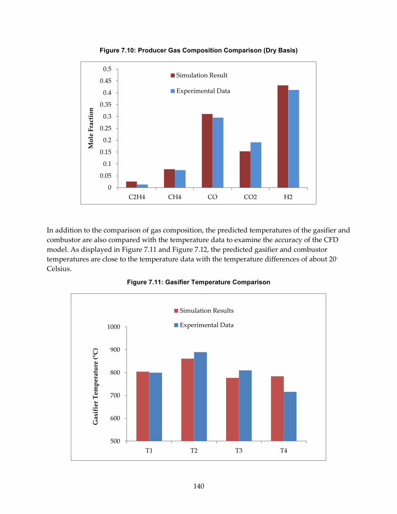
Figure 7.10: Producer Gas Composition Comparison (Dry Basis)

In addition to the comparison of gas composition, the predicted temperatures of the gasifier and combustor are also compared with the temperature data to examine the accuracy of the CFD model. As displayed in Figure 7.11 and Figure 7.12, the predicted gasifier and combustor temperatures are close to the temperature data with the temperature differences of about 20◦ Celsius.

Figure 7.11: Gasifier Temperature Comparison

0

0.05

0.1

0.15

0.2

0.25

0.3

0.35

0.4

0.45

0.5

C2H4 CH4 CO CO2 H2

Mol

e Fr

actio

n

Simulation Result

Experimental Data

500

600

700

800

900

1000

T1 T2 T3 T4

Gas

ifie

r Tem

pera

ture

(°C

)

Simulation Results

Experimental Data

140

Figure 7.12: Combustor Temperature Comparison

6.1.7 Analysis of Model In this work the MP-PIC method was applied to simulate biomass gasification in a dual fluidized-bed system. The predicted gas composition and reactor temperature profiles were compared with the experimental data to validate the model, and good agreement was achieved.

The studies of mesh resolution and computational particle number were implemented and the temperature and composition profiles predicted from these case studies were similar. The base case with the 243,423-cell grid and 419,506 computational particles was chosen for the remaining studies producing acceptable accuracy while minimizing computing cost.

The effect of particle size distribution (PSD) was investigated. At bottom region of the combustor, the solid volume fraction predicted from the case with 𝜎𝜎 = 0.3𝑑𝑑𝑙𝑙 is higher than those of the cases with 𝜎𝜎 = 0.2𝑑𝑑𝑙𝑙 and monodisperse particles, which indicates that the impact of PSD is significant in the lower region.; however, the study also shows that in the upper region the impact of PSD becomes insignificant, and the solid volume fractions for the three cases are similar. This is principally because at the current hydrodynamic conditions the large particles in the PSD cannot easily reach the upper region of the combustor to change the flow pattern.

The impact of drag model was analyzed. Three cases using the Wen-Yu, Turton-Levenspiel, and energy minimization multi-scale (EMMS) models were examined. The predicted distributions of solid volume fraction and particle velocity from three cases were compared, and it was found that the effect of drag models was not significant on the flow patterns of the system. The EMMS

500

550

600

650

700

750

800

850

900

950

1000

T7 T8 T9 T10

Com

bust

or T

empe

ratu

re (°

C)

Simulation Results

Experimental Data

141

drag model predicted more clustering particles than others. Consequently, the solid volume fraction predicted by the EMMS model was denser and the velocity was smaller than those of other drag models.Further details on these performance of the MP-PIC model is available in the published version of the study (Liu, 2015).

6.1.7.1 Application to Commercial Scale BCHP Plants The MP-PIC method for the three dimension full loop simulation of dual fluidized bed biomass gasifier applied at the pilot scale in this study has successfully produced experimental performance. It can be used to simulate large demonstration commercial scale systems. This is a very valuable tool for design studies of the performance of commercial systems and can be used to lower the risk in scaling the design from pilot to commercial scale.

6.8 BCHP Life Cycle Model A life cycle inventory for a 3 MWe biomass gasification system using biomass produced through the production of almonds in California was created. The basis for the analysis is from the lifecycle cost analysis performed by Kendall et al on almond production in California and a lifecycle analysis of a forest based BCHP design. The analysis presented here considers greenhouse gases and criteria air pollutants considered in the Kendall et al analysis (PM2.5, NMVOC, CO, NOx and SO2).

6.8.1 Model Description The environmental burden for almond shells, almond prunings and biomass from almond orchard removals was determined using an economic allocation method and the almond system lifecycle cost analysis in Kendall et al (submitted). The economic allocation used in Kendall et al assumed a $3.53/dry ton value for biomass used for energy at the point of production – shelling facility for shells and the orchard for the prunings and orchard removals. We modified this to $30/dry ton biomass used in energy production that will need to compete with alternate uses of the biomass. Almond shells currently have a market value of roughly $30/ton (AHPA, 2015, personal communication). Biomass destined for energy production provides 0.6% of the economic value of the almond production system. The total emissions from the almond production system on a per-hectare of orchard were multiplied by this factor and divided by the lifetime production of biomass for a hectare of almond orchard to find the emissions associated with the production of biomass.

The transportation of biomass from the orchards to the gasification plant were calculated using GREET 1_2014 for the emissions from the operation of a 25 ton truck. The one-way distance from the orchard to the gasification facility is assumed to be 33.6 km based on the average distance from current almond orchards to existing biopower facilities. This distance could be shorter if facilities are co-located with almond processing facilities. The almonds are hauled 26.7 km on average to a processing facility. (Kendall, et al, submitted) An empty back haul is included in the emissions calculation.

The gasification facility is modeled after a 10 MWe gasification-based CHP facility described in Francois et al (2014). The facility is assumed to have an efficiency of 24%. The criteria air pollutant emissions were taken to be the minimum of the estimates from the study and the

142

emissions for new reciprocating engines in California. Due to the higher NOx standards in California the NOx emissions were reduced from 0.76 g/kWh to 0.23 g/kWh. The CO emissions were also reduced from 3.1 g/kWh to 1.9 g/kWh.

Criteria air pollutants are calculated and reported on a g/kWh basis. Greenhouse gas (GHG) emissions are standardized in units of CO2-equivalence (CO2e) based on the most recent Intergovernmental Panel on Climate Change’s global warming potentials (GWP) (Myhre et al. 2013).

The California grid mix emissions are estimated using CA-GREET 2.0 with a grid mix as described in Table 7.13 which is the grid mix for California in 2010 as reported by California Environmental Protection Agency’s (EPA) eGRID database. CA-GREET 2.0 gives the emissions for each source of electricity in the California context.

Table 7.13: California Grid Mix

California Grid Mix from eGRID 2010 Natural Gas 51% Hydroelectric 15% Nuclear 15% Coal 7% Geothermal 4% Wind 3% Biomass 3% Residual Oil 1% Solar PV 0% Others 0%

6.8.2 Model Performance Electricity generated from almond biomass using the BCHP system is projected to have a much lower contribution to greenhouse gases than the current electricity grid mix. Using the 20-year global warming potential, the BCHP system is projected to have 70% lower emissions than the current grid mix. Stretching the time horizon out to 100 years, the BCHP system has a 67% lower emissions than the current grid mix. 92% of the emissions contributing to the global warming impact occur at the conversion stage of the system.

143

Table 7.14: Summary of Greenhouse Gases and Criteria Air Pollutant Emissions for Almond Biomass BCHP

Emissions of greenhouse gases and criteria air pollutants (g/kWh produced)

Emissions Biomass upstream

Biomass transport Conversion

Biogenic

Carbon Total CA Grid

mix CO2 3.82 3.315 1,546.17 -1428.75 124.55 363.82 N2O 0.00895 3.51E-06 0.01 0.02 0.01 CH4 0.0182 0.000817 - 0.02 0.99 GWP20 7.70 3.375 1,550.42 -1428.75 132.75 437.86 GWP100 6.97 3.337 1,550.55 -1428.75 132.11 391.65 PM2.5 0.0646 6.44E-05 0.03 0.09 0.04 NMVOC 1.31 0.000714 0.002 1.32 0.06 CO 0.0672 0.002949 1.94 2.01 0.39 NOx 0.0259 0.008335 0.23 0.26 0.54 SO2 1.28 2.86E-05 0.17 1.45 0.42

The results on criteria air pollutants are more mixed. The BCHP system is estimated to have much higher lifecycle emissions of VOCs, CO, and SOx. The system is also expected to have more than double the PM2.5 emissions. On the other hand, the BCHP system demonstrates an improvement in NOx emissions compared to the current grid mix. It is important to note that these estimates do not include exposure impacts. A higher emitting pathway can have a lower impact if located away from population and/or in an area with less critical air quality problems.

6.9 BCHP Economic Model Describes a pro forma economic model for a commercial scale BCHP plant based on demonstration scale performance and commercial scale system design.

6.9.1 Model Basis A model to study the economic feasibility of the development of renewable energy generation in California using BCHP plants was developed. The BCHP technology to be evaluated is based on collaboration between the University of California and West Biofuels to demonstrate robust, efficient, and environmentally sound power production from a BCHP system that can be commercially deployed in the agricultural processing sector in California. To evaluate the economic feasibility the BCHP gasification technology, a pro forma economic model was developed for a commercial-scale (3 MWe) BCHP plant. This model was based on a commercial-scale system design using performance data from the West Biofuels demonstration-scale (250 kWe) power plant at the WB RC. The economic feasibility model analysis incorporates tax credits and incentives for renewable energy that are either available, or are expected to be available in the near future in California.

144

6.9.2 Model Description The economic analysis was preformed according to the Capital Assets Pricing Model that is typically used for factory or power-plant type capital assets that produce revenue. As with any economic projection, this analysis requires and relies upon a number of technical assumptions. These assumptions were made based upon operations of the demonstration-scale plant and were scaled appropriately for a commercial-scale system and on the financial credits and incentives provide for renewable power systems. Four principal economic scenarios were evaluated in the model: (1) base case no credits or incentives, (2) New Market Tax Credit (NMTC), (3) Electric Program Investment Charge (EPIC), and (4) Combined NMTC and EPIC. A description of NMTC and EPIC follows:

6.9.2.1 New Market Tax Credit (NMTC) The New Market Tax Credit (NMTC) is designed to support development in disadvantaged communities. These communities are defined by census tracts that either have over 20% of the population below the poverty level or have a median income that does not exceed the median income of 80% of the state. This typically employs a leveraged structure, with approximately 30% of the funds contributed from the tax credit investor. In return for this investment, the tax credit investor receives a tax credit worth 39% of the NMTC fund over the next seven years (5% credit for the first three years, 6% credit for the last four years). The Qualified Active Low-Income Community Business (QALICB) receiving these funds generally makes interest payments during this period, but is precluded from paying off the principle portion of this debt while the tax credit is being claimed by the tax credit investor.

A common NMTC structure involves a loan and a tax credit investment combining in a NMTC fund. The 39% tax credit is based upon the total value of this fund. This fund is managed by a Community Development Entity (CDE). The CDE generally charges management fees worth between 5-10% of the value of the NMTC fund. The CDE discharges funds to the QALICB, which uses these funds for project costs. This potential structure is illustrated in Figure 7.13.

Typically, the tax credit investor has a put option that can be exercised at the end of the project’s seventh year. This option, if exercised, allows the QALICB to purchase the tax credit investor’s portion of the fund for a nominal amount of approximately $1,000. This allows the QALICB to effectively have that portion of the debt forgiven. Depending on the asset value of the project at the time of exercise of the put option there may or may not be a taxable gain. This generally results in a taxable gain. Altogether, this credit can effectively reduce the cost of a project by about 10%.

More information can be found on the Internal Revenue Service’s website: http://www.irs.gov/pub/irs-utl/atgnmtc.pdf.

145

Figure 7.13: New Market Tax Credit Financial Structure

6.9.2.2 Electric Program Investment Charge (EPIC) The Electric Program Investment Charge (EPIC) is funded by an Investor-Owned Utility (IOU) ratepayer surcharge. This program is designed to promote development of pre-commercial renewable energy projects. EPIC grants can range from $2-5 million. These funds can be invoiced to offset capital costs. More information can be found at the California Energy Commission website: http://www.energy.ca.gov/research/epic/.

6.9.2.3 SB 1122 Feed-in Tariff The SB 1122 feed-in tariff is intended to support the production of clean energy by offering contracts to energy production facilities under 3MW in size. These contracts can be for 10, 15, or 20 years in duration. While this tariff has not been finalized, initial contract offers are expected to be approximately $124.66/MWh.

This initial price will be adjusted by a mechanism modeled after the Renewable Market Adjusting Tariff (ReMAT). Once every two months, contracts will be offered. If there are more than five qualified producers and 20% or fewer of contracts are accepted, the price will increase the next time contracts are offered. The amount of this increase will grow in size if consecutive offerings result in less than 20% acceptance. The size of the first increase is $4/MWh. The second consecutive increase is $8/MWh. Increases are capped at $12/MWh for three or more consecutive offerings with less than 20% acceptance. Similarly, with five or more qualifying projects, 100% acceptance will result in a rate decrease. This decrease will be $4/MWh for the first such period, then $8/MWh and $12/MWh respectively for consecutive periods as above.

6.9.2.4 Base Case Economic Assumptions The base case economic analysis follows some general assumptions in terms of operating parameters and the development schedule:

146

For the project development a year is spent ensuring that all closing costs for NMTC and SB 1122 are paid and permitting is in place. This is designated year 0. Construction starts the next year and continues for 18 months. The second half of the second year is spent commissioning and optimizing plant operations. If EPIC funds are acquired, they are used in the first year to offset construction costs.

It is assumed that it is not possible to include EPIC funds into a NMTC fund, effectively reducing the size of the NMTC gain when EPIC funding is acquired. Income and regular operating costs begin in year three. If a NMTC financing structure is employed, any gain from the exercise of the put option occurs in year seven. The genset is refurbished for half the cost of a new genset in the tenth year of operation. The gasifier has a usable life of 20 years and equipment was depreciated according to a 5-year modified accelerated cost recovery system (MACRS) schedule.

The assumptions made in the base case scenario are presented in Table 7.13. Yearly inflation of all costs and revenues other than revenue from electricity was assumed to be 2.1%. Yearly revenue from electricity was held constant because it is dependent upon a SB 1122 contract. For the purposes of these calculations, a 20 year contract is assumed. Yearly inflation of all costs and revenues other than revenue from electricity was assumed to be 2.1%. Yearly revenue from electricity was held constant because it is dependent upon a SB 1122 contract. For the purposes of these calculations, a 20 year contract is assumed. A 40% tax rate is assumed.

Assumptions for the feedstock are a cost of $20/dry-ton and a LHV of 17.3 MJ/dry-ton. The gasifier efficiency is 70% and that of the electrical generator set 32.8%. This gives an overall efficiency of 22.9% from biomass (LHV) to electricity, or a heating rate of 14,875 Btu to generate one kWh of electricity. Under these assumptions, a dry ton of biomass generates 1 MWh of electricity. Therefore, the feedstock cost can also be expressed in $20/MWh or $1.345/thousand British thermal units (Btu).

147

Table 7.15: Base Case Economic Assumptions

6.9.3 Economic Analysis In the analysis the following economic terms will be used:

Present Value – The value of future cash flows discounted to account for alternate opportunities for investment funds in the present.

NPV – “Net Present Value” – The sum of the present value of cash flows for all years of a project’s life.

WACC – “Weighted Average Cost of Capital” - The rate at which future cash flows are discounted when calculating present value. For the calculation, WACC = (portion of financing from equity)*(return on equity) + (debt interest rate)*(portion of financing from debt)*(1-tax rate).

ROE - Return on Equity – The rate of profit that investors demand from their investment.

Assumption Category Value

Return on Equity 20%Debt interest rate 5%Percentage of financing from debt 80%Resulting WACC 6.4%

SB1122 closing costs $500,000Yearly electricity production 23,000 MWhPrice of heat $4/mmBTUAmount of heat utilized 156,837 mmBTUAuction value of cap and trade benefits (per ton of carbon reduced)

$10.00

Tons of carbon reduction 26,806 tonsLabor Costs $600,000/yearIncremental cost of feedstock $20/dry-tonOther operating costs $100,000/yearGasifier construction costs $10.5 millionGenset construction costs $4.5 millionHeat recapture equipment $450,000Gasifier maintenance $525,000/yearGenset maintenance $450,000/year

Lower heating value 17.3 MJ/dry-tonGasifier efficiency 70%Genset efficiency 32.80%Overall efficiency 22.90%Heating Rate (to generate 1 kWh electricity) 14,875 BTU(th)Electricity generated from 1 dry-ton biomass 1 MWh

Assumptions Made for Base Case

148

LCOE – “Levelized Cost of Energy” – The price of electricity that results in an NPV of 0. This is calculated as the present value of all costs divided by the present value of all electricity production.

In the economic analysis the four basic scenarios were examined: a scenario where no incentives, a scenario utilizing the NMTC, a scenario utilizing EPIC funding, and a scenario utilizing both the NMTC and EPIC funding. Unless otherwise noted, the discount rate and other economic assumptions used are those of the base case described in Table 7.15. The base case cost for the BCHP 3 MWe plant (largest allowable under SB 1122) from Table 7.15 is taken as $16 million. The comparison of the LCOE for the four scenarios is presented in Table 7.16.

Table 7.16: Comparison of the LCOE for BCHP Production with Various Credit and Investment Scenarios

BCHP Project Financial Scenarios LCOE ($/MWh) Base Case No-Incentives 160.2 New Market Tax Credit 149.0 Energy Program Investment Charge 125.4 NMTC and EPIC 118.3

6.9.4 No Incentives Scenario: As mentioned above, discounted cash flows were used to determine the NPV of each scenario. The LCOE was calculated as the present value of all costs divided by the present value of the volume of electricity generated. In the absence of incentives, the LCOE that is calculated using these base assumptions is $160.20/MWh.

6.9.4.1 NMTC-only Scenario: Setting up the NMTC fund requires closing costs that must be spent in year 0. These are assumed to be $500,000. If the NMTC is utilized without EPIC funding, the NMTC fund size is equal to the entire cost of construction. For the sake of cash flow calculations, it is assumed that the put option is exercised, resulting in a taxable gain of $4,635,000 in year seven of the project. This lowers the LCOE to $149.00/MWh. Thus, the incremental decrease in LCOE from using the NMTC is $11.20/MWh.

6.9.4.2 EPIC-only Scenario: For this scenario, a grant size of $5 million is assumed. This grant is used to offset construction costs in the first year. This reduces the LCOE to $125.14/MWh. Thus, the maximum incremental decrease in LCOE from using EPIC funding is $35.05/MWh.

6.9.4.3 NMTC+EPIC Scenario: When both NMTC and EPIC are utilized, it is assumed that the EPIC funds cannot be included in the NMTC fund. This effectively reduces the fund size by $5 million. The resulting gain in year seven is $3,135,000. This scenario results in a LCOE of $118.29/MWh.

Thus, the incremental decrease from using both of these incentives in combination is $41.90/MWh.

149

6.9.4.4 Comparison to Black and Veatch Model As part of the application for EPIC funds, applicants are required to use the SB 1122 Levelized Cost of Electricity Calculator developed by Black and Veatch for the California Public Utilities Commission (http://www.cpuc.ca.gov/NR/rdonlyres/69848D0B-9EA3-466B-8B8F-CE1E0EEF1894/0/PublicDRAFTLCOEModelCPUCSB 1122.xlsx). This model was compared with our pro forma using the base settings of each model. Table 7.17 summarizes the comparison of the Black and Veatch default scenarios with the base case scenario used in the pro forma. The estimates and assumptions used in the pro forma were converted to the format used in the Black and Veatch model for this comparison.

The Black and Veatch model for calculating the LCOE allows selection of technology type and cost level. Using the base settings for the Forest/Agricultural Residues case, the respective low, the principal changes in these settings are capital cost, operating costs, fuel cost, heat rate, and capacity factor. These calculations were done in the absence of incentives.

150

Table 7.17: Comparison of LCOE from Black and Veatch Model to Base Case Model

The assumptions in the base case of the pro forma are very similar to those in the Black and Veatch scenarios. Most of the engineering estimates used in the no-incentive scenario in the pro forma are on the low end of the range of the Black and Veatch model, but all are still higher than the “low” setting. The differences that are most likely to be significant are some of the financial assumptions. For the base case, 80% of project funding comes from debt, at a 5% interest rate, and no principle is paid off until the end of the debt term. The cost of equity is also estimated to be twice that in the Black and Veatch model. The base case pro forma also includes a cap and trade benefit from carbon reduction. The resulting LCOE of the pro forma base case is $160.20/MWh, $38.27/MWh less than the “medium” Black and Veatch estimate and $26.21/MWh above the “low” Black and Veatch estimate for Forest/Agricultural Residues.

Pro Forma Base CaseCategory

Low Medium High

Project Capacity (MW) 3 3 3 3Capital Cost ($/kW) 5000 6000 7500 5317Fixed O&M ($/kW) 347 553 590 387Fixed O&M Escalation 2% 2% 2% 2.10%Variable O&M ($/MWh) 0 0 0 0Variable O&M Escalation 0% 0% 0% 0%Fuel Cost ($/mmBTU) 1.11 1.67 2.22 1.35Fuel Cost Escalation 2% 2% 2% 2.1%Heat Rate (BTU/kWh) 15000 16500 18000 14875Capacity Factor 0.9 0.85 0.8 0.9

Financial EntriesDebt Percentage 60% 60% 60% 80%Debt Rate 7% 7% 7% 5%Debt Term (years) 15 15 15 20Economic Life (years) 20 20 20 20Depreciation Term (years) 7 7 7 5Percent Depreciated 100% 100% 100% 100%Cost of Generation Escalation 0% 0% 0% 0%Tax Rate 40% 40% 40% 40%Cost of Equity 10% 10% 10% 20%Discount Rate 7% 7% 7% 6.4%

IncentivesPTC ($/MWh) 0 0 0 0PTC Escalation 0% 0% 0% 0%PTC Term (years) 0 0 0 0ITC 0% 0% 0% 0%Other Incentives ($/year) 0 0 0 $268,064.93Incentive Escalation (%) 0% 0% 0% 2.1%

LCOE $133.99 $198.47 $251.04 $160.20

SettingsBlack and Veatch Model

151

6.9.5 Model Performance Since there are many assumptions that go into the analysis of the economic feasibility of the proposed BCHP plant, it is important to understand the sensitivity of these assumptions upon the analysis. To determine the relative importance of the assumptions involved in the economic analysis the project financial parameters described in the base case in Table 7.15 were varied to determine the effect on the base case LCOE as well as the effect when including NMTC and/or EPIC funding. The specific financial parameters that varied were: construction cost, heat price, fuel cost, interest rate, return on equity, and discount rate. The analyses is based on the LCOE that will produce a NPV=0 satisfying the financial assumptions. The resulting LCOE values are described in the following summaries.

6.9.5.1 Construction Cost The cost of construction varied by $2 million above and below that of the base case. This resulted in an overall cost of construction between approximately $14 million and $18 million. In addition to affecting the initial funding required to begin the project, this change also proportionally affects any NMTC-related gain recognized in year seven. The results of the sensitivity analysis on the LCOE are presented in Table 7.18.

Table 7.18: Sensitivity Analysis of Capital Cost – LCOE Summary

The no-incentive scenario resulted in a LCOE that ranged between $141.30/MWh and $179.09/MWh. The incremental change in LCOE caused by a $2 million change in cost of construction was $18.89/MWh. In the NMTC-only scenario, the incremental change in LCOE from a $2 million change in cost of construction was $17.15/MWh. This resulted in a LCOE range of $131.84/MWh to $166.15/MWh. The incremental change in the EPIC-only scenario was $18.89, identical to that of the no-incentives scenario. The resulting LCOE ranged from $106.25/MWh to $144.03/MWh. In the NMTC + EPIC scenario, the incremental change in LCOE caused by a $2 million change in construction cost was $17.15, identical to that of the NMTC-only scenario and resulted in a LCOE ranging from $101.14/MWh to $135.44/MWh.

6.9.5.2 Heat Price The price of the waste heat that is capable of utilization was varied from the base value of $4/mmBtu to $6/mmBtu, $8/mmB, and $10/mmB respectively. These higher prices reflect scenarios that recognize additional benefit beyond the replacement of natural gas costs. The results of the sensitivity analysis of Heat Price on the LCOE are presented in Table 7.19.

LCOE (varied Capital Cost) $14MM $16MM $18MMNo-Incentives Scenario 141.30 160.20 179.09NMTC-only Scenario 131.84 149.00 166.15EPIC-only Scenario 106.25 125.14 144.03NMTC + EPIC Scenario 101.14 118.29 135.44

152

Table 7.19: Sensitivity Analysis of Heat Price – LCOE Summary

• For the no-incentive scenario, the incremental change in LCOE caused by a $2/mmBtu change in heat price was $16.20/MWh. Increasing heat prices caused a reduction in the LCOE. From lowest to highest heat price, the LCOE was $160.20/MWh, $143.99/MWh, $127.79/MWh, and $111.59/MWh respectively.

• For the NMTC-only scenario, the incremental change in LCOE resulting from a $2/mmBtu change in heat price was $16.20/MWh, identical to every other scenario. The LCOE was $149.00/MWh, $132.80/MWh, $116.59/MWh, and $100.39/MWh.

• For the EPIC-only scenario, the incremental change in LCOE due to a $2/mmBtu change in heat price was $16.20/MWh. The LCOE was $125.14/MWh, $108.94/MWh, $92.74/MWh, and $76.54/MWh.

• For the NMTC+EPIC scenario, the incremental change in LCOE due to a $2/mmBtu change in heat price was $16.20/MWh. The LCOE was $118.29/MWh, $102.09/MWh, $85.89/MWh, and $69.69/MWh.

It is clear from this analysis that an increased value of the utilization of waste heat as a replacement for natural gas has a significant effect on the LCOE and the ultimate ROE of a BCHP project.

6.9.5.3 Fuel Cost The starting cost of feedstock was varied from the base case of $20/dry-ton to $30/dry-ton, $40/dry-ton, and $50/dry-ton, respectively. With a plant efficiency of 23%, the cost of feedstock per dry-ton equals the cost per generated MWh. Higher fuel costs represent both added incremental harvest costs and scenarios where feedstock must be purchased from external sources. The results of the sensitivity analysis of Fuel Cost on the LCOE are presented in Table 7.20.

LCOE (varied Heat Price) $4/mmBTU $6/mmBTU $8/mmBTU $10/mmBTUNo-Incentives Scenario 160.20 143.99 127.79 111.59NMTC-only Scenario 149.00 132.80 116.59 100.39EPIC-only Scenario 125.14 108.94 92.74 76.54NMTC + EPIC Scenario 118.29 102.09 85.89 69.69

153

Table 7.20: Sensitivity Analysis of Fuel Costs – LCOE Summary

• In the no-incentive scenario, the incremental change in LCOE that results from a $10/MWh ($10/dry-ton) change in fuel cost was $11.88/MWh. The change in LCOE was larger than the change in fuel cost because the cost of fuel is subject to inflation, but the price of electricity is held constant by a SB 1122 contract. From lowest to highest fuel cost, the LCOE was $160.20/MWh, $172.07/MWh, $183.95/MWh, and $195.83/MWh.

• In the NMTC-only scenario, the incremental change in LCOE that resulted from a $10/MWh ($10/dry-ton) change in fuel cost was $11.88/MWh also. From lowest to highest fuel cost, the LCOE was $149.00/MWh, $160.88/MWh, $172.75/MWh, and $184.63/MWh respectively.

• In the EPIC-only scenario, the incremental change in LCOE that resulted from a $10/MWh ($10/dry-ton) change in fuel cost was, again, $11.88/MWh. From lowest to highest fuel cost, the LCOE was $125.14/MWh, $137.02/MWh, $148.90/MWh, and $160.78/MWh.

• In the NMTC+EPIC scenario, the incremental change in LCOE that resulted from a $10/MWh ($10/dry-ton) change in fuel cost was $11.88/MWh also. From lowest to highest fuel cost, the LCOE was $118.29/MWh, $130.17/MWh, $142.05/MWh, and $153.93/MWh.

The sensitivity analysis on Fuel Costs demonstrates the importance of controlling feedstock price over the life of the project.

6.9.5.4 Interest Rate The scenarios derived from the base case were financed by a significant portion of debt (80%). This could result in a perceived risk of default and a higher interest rate than is currently assumed. In the base case, the interest rate was set at 5%. To determine the sensitivity of the LCOE to this assumption, the rate was varied from 3% to 10%. The interest rate is one of the factors that influence the WACC. Other factors with the potential to influence the WACC such as return on equity and percentage of financing from debt were held constant at the base case values. The results of the sensitivity analysis of Interest Rate on the LCOE are presented in Table 7.21.

LCOE (varied Fuel Cost) $20/dry-ton $30/dry-ton $40/dry-ton $50/dry-tonNo-Incentives Scenario 160.20 172.07 183.95 195.83NMTC-only Scenario 149.00 160.88 172.75 184.63EPIC-only Scenario 125.14 137.02 148.90 160.78NMTC + EPIC Scenario 118.29 130.17 142.05 153.93

154

Table 7.21: Sensitivity Analysis of Interest Rate – LCOE Summary

Changing the interest rate had a greater effect on the LCOE when the magnitude of the interest rate was larger.

• For the no-incentive scenario, the incremental change in LCOE was $3.56/MWh when the interest rate changed from 3% to 4%. When the interest rate changed from 9% to 10%, the incremental change in LCOE was $4.12/MWh. From lowest to highest interest rate, the LCOE was $152.97/MWh, $156.54/MWh, $160.20/MWh, $163.95/MWh, $167.80/MWh, $171.74/MWh, $175.78/MWh, and $179.90/MWh respectively.

• For the NMTC-only scenario, the incremental change in LCOE was $3.43/MWh when the interest rate changed from 3% to 4%. When the interest rate changed from 9% to 10%, the incremental change in LCOE was $4.06/MWh. The LCOE was $142.02/MWh, $145.45/MWh, $149.00/MWh, $152.64/MWh, $156.39/MWh, $160.24/MWh, $164.20/MWh, and $168.25/MWh

• For the EPIC-only scenario, the incremental change in LCOE was $2.10/MWh when the interest rate changed from 3% to 4%. When the interest rate changed from 9% to 10%, the incremental change in LCOE was $2.44/MWh. The LCOE was $120.89/MWh, $122.99/MWh, $125.14/MWh, $127.35/MWh, $129.62/MWh, $131.94/MWh, $134.33/MWh, and $136.76/MWh.

• For the NMTC + EPIC scenario, the incremental change in LCOE was $2.04/MWh when the interest rate changed from 3% to 4%. When the interest rate changed from 9% to 10%, the incremental change in LCOE was $2.43/MWh. The LCOE was $114.14/MWh, $116.19/MWh, $118.29/MWh, $120.46/MWh, $122.70/MWh, $125.00/MWh, $127.37/MWh, and $129.80/MWh.

6.9.5.5 ̀ Return on Investment (ROI) A major factor that contributes to the WACC is the return on equity (ROE) demanded by investors. Similar to the interest rate for debt, the return demanded by investors can increase with the perceived risk of default. In the base case, the return on equity was set at 20%. This rate was varied up to 60% return on equity at intervals of 10%. Other factors with the potential to influence the WACC, such as interest rate and percentage of financing from debt, were held constant at their base case values. The results of the sensitivity analysis of Return on Equity on the LCOE are presented in Table 7.22.

LCOE (varied Interest Rate) 3% 4% 5% 6% 7% 8% 9% 10%No-Incentives Scenario 152.97 156.54 160.20 163.95 167.80 171.74 175.78 179.90NMTC-only Scenario 142.02 145.45 149.00 152.64 156.39 160.24 164.20 168.25EPIC-only Scenario 120.89 122.99 125.14 127.35 129.62 131.94 134.33 136.76NMTC + EPIC Scenario 114.14 116.19 118.29 120.46 122.70 125.00 127.37 129.80

155

Table 7.22: Sensitivity Analysis of Return on Investment – LCOE Summary

Changing the return on equity had a greater effect on the LCOE when the magnitude of the return was larger.

• For the no-incentive scenario, the incremental change in LCOE was $16.26/MWh between 20 and 30% return on equity. The incremental change in LCOE between 50 and 60% was $20.92/MWh. From lowest to highest return on equity, the LCOE was $160.20/MWh, $176.46/MWh, $194.32/MWh, $213.75/MWh, and $234.67/MWh.

• For the NMTC-only scenario, the incremental change in LCOE was $15.87/MWh between 20 and 30% return on equity. The incremental change in LCOE between 50 and 60% was $21.05/MWh. From lowest to the highest return on equity, the LCOE was $149.00/MWh, $164.87/MWh, $182.51/MWh, $201.89/MWh, and $222.93/MWh.

• For the EPIC-only scenario, the incremental change in LCOE was $9.58/MWh between 20 and 30% return on equity. The incremental change in LCOE between 50 and 60% was $12.46/MWh. From lowest to highest return on equity, the LCOE was $125.14/MWh, $134.73/MWh, $145.29/MWh, $156.82/MWh, and $169.28/MWh.

• For the NMTC+EPIC combined scenario, the incremental change in LCOE was $9.47/MWh between 20 and 30% return on equity. The incremental change in LCOE between 50 and 60% was $10.59/MWh. From lowest to highest return on equity, the LCOE was $118.29/MWh, $127.77/MWh, $138.35/MWh, $150.04/MWh, and $162.80/MWh.

6.9.5.6 Discount Rate (WACC) For the base case, a calculated WACC was used as the discount rate for all present value calculations. The calculation assumed a 20% return on equity, 5% interest rate, and 80% debt financing. The resulting WACC was 6.4%. To determine the effect of less optimistic financial assumptions, the discount rate was varied between 6% and 16% at 2% intervals. This range was chosen because it approximated the range of the WACC calculated from the possible combinations of return on equity and debt interest rates used above. The calculated WACC from each potential financing situation is summarized in Table 7.23.

LCOE (varied ROE) 20% 30% 40% 50% 60%No-Incentives Scenario 160.20 176.46 194.32 213.75 234.67NMTC-only Scenario 149.00 164.87 182.51 201.89 222.93EPIC-only Scenario 125.14 134.73 145.29 156.82 169.28NMTC + EPIC Scenario 118.29 127.77 138.35 150.04 162.80

156

Table 7.23: WACC on ROE and Debt Interest Rate (80% Financing)

The results of the sensitivity analysis of WACC on the LCOE are presented in Table 7.24.

Table 7.24: Sensitivity Analysis of WACC – LCOE Summary

The incremental change in LCOE caused by a 2% change in discount rate depends upon the magnitude of the discount rate. This makes sense because with higher power prices, more revenue is generated. With more revenue, higher discount rates result in higher absolute values of these discounts, resulting in a higher LCOE.

• In the no-incentives scenario, the difference in the LCOE between using a 6% discount rate and an 8% discount rate was $15.93/MWh. The difference between the LCOE between calculations using a 14% discount rate and a 16% discount rate was $22.07/MWh. Thus, from lowest to highest discount rate, the LCOE was $157.14/MWh, $173.07/MWh, $190.62/MWh, $209.74/MWh, $230.37/MWh and $252.44/MWh respectively.

• In the NMTC-only scenario, the difference in the LCOE between calculations using a 6% discount rate and an 8% discount rate was $15.51/MWh. The difference between the LCOE using a 14% discount rate and a 16% discount rate was $22.34/MWh. Thus, from

20% 30% 40% 50% 60%3% 5.44% 7.44% 9.44% 11.44% 13.44%4% 5.92% 7.92% 9.92% 11.92% 13.92%5% 6.40% 8.40% 10.40% 12.40% 14.40%6% 6.88% 8.88% 10.88% 12.88% 14.88%7% 7.36% 9.36% 11.36% 13.36% 15.36%8% 7.84% 9.84% 11.84% 13.84% 15.84%9% 8.32% 10.32% 12.32% 14.32% 16.32%10% 8.80% 10.80% 12.80% 14.80% 16.80%

Sensitivity of WACC to Return on Equity and Debt Interest Rate

Return on EquityDe

bt In

tere

st R

ate

LCOE (varied WACC) 6% 8% 10% 12% 14% 16%No-Incentives Scenario 157.14 173.07 190.62 209.74 230.37 252.44NMTC-only Scenario 146.04 161.55 178.84 197.88 218.59 240.93EPIC-only Scenario 123.35 132.73 143.10 154.44 166.72 179.90NMTC + EPIC Scenario 116.53 125.78 136.15 147.62 160.16 173.75

157

lowest to highest discount rate, the LCOE was $146.04/MWh, $161.55/MWh, $178.84/MWh, $197.88/MWh, $218.59/MWh, and $240.93/MWh.

• In the EPIC-only scenario, the difference in the LCOE from calculations using a 6% discount rate and those using an 8% discount rate was $9.38/MWh. The difference between the LCOE using a 14% discount rate and one using a 16% discount rate was $13.18/MWh. Thus, from lowest to highest discount rate, the LCOE was $123.35/MWh, $132.73/MWh, $143.10/MWh, $154.44/MWh, $166.72/MWh, and $179.90/MWh respectively.

• In the NMTC + EPIC scenario, the difference in the LCOE using a 6% discount rate and one using an 8% discount rate was $9.25/MWh. The difference between the LCOE using a 14% discount rate and one using a 16% discount rate was $13.58/MWh. Thus, from lowest to highest discount rate, the LCOE was $116.53/MWh, $125.78/MWh, $136.15/MWh, $147.62/MWh, $160.16/MWh, and $173.75/MWh respectively.

6.9.6 Conclusions: From the sensitivity analysis that was conducted, reducing the cost of construction prior to income-generation is the most effective way to reduce the LCOE. Increasing the effective price of the waste heat that is re-captured would also be similarly effective.

The most effective incentive is a maximum-value EPIC grant. In the context of the results from the sensitivity analysis, this is because the EPIC money can be applied directly to construction costs, which is the most effective way to reduce the LCOE.

The New Market Tax Credit can also be useful to reducing the LCOE, but not as effective as an EPIC grant. This is largely due to fact that the benefit from the New Market Tax Credit is spread over a seven year period, whereas the EPIC funds are used in year one. Employing the NMTC structure is useful for amassing the initial required financing.

Commencement of this type of project will require SB 1122 to be enacted, since the LCOE for all of these scenarios is much higher than the rate electricity generators would be able to receive otherwise in the current market. However, these projects could still be delayed for at least several months after SB 1122 is enacted, depending upon whether the NMTC and/or EPIC funding can utilized.

6.9.7 Evaluation of Commercial Scale BCHP Systems The financial performance of the base case scenario for a 3 MWe BCHP plant, including sensitivity to the financial assumptions, was presented in the previous section. With that as a background, the economic feasibility of a BCHP system for use in the California agricultural processing sector is closely tied to implementation of the proposed SB 1122 feed-in-tariff system.

Using the base case LCOE results for the four scenarios presented in Table 7.16 and the schedule for the implementation of SB 1122 contract price, the feasibility of a BCHP project participating in SB 1122 for each of the scenarios is presented in Table 7.25 and the NPV associated with increasing contract price is presented in Table 7.26.

158

Table 7.25: Schedule of Potential SB 1122 Contract Acceptance Prices

Table 7.25 presents the feed-in tariff contract price that is possible at each offering for the first two years following the beginning of SB 1122 auctions. This assumes that the rate of $124.66/MWh is the initial price offered, as currently proposed. This also assumes that fewer than 20% of contracts are accepted and that there are enough potential projects to qualify for a rate increase for each subsequent period.

Month Contract Price First Opportunity for Contract Acceptance0 $124.66/MWh NMTC+EPIC Scenario2 $128.66/MWh EPIC-only Scenario4 $136.66/MWh6 $148.66/MWh8 $160.66/MWh NMTC-only Scenario10 $172.66/MWh No-Incentive Scenario12 $184.66/MWh14 $196.66/MWh16 $208.66/MWh18 $220.66/MWh20 $232.66/MWh22 $244.66/MWh24 $256.66/MWh

Maximum Rate of SB1122 Contract Price Increase

159

Table 7.26: Projected NPV for the Four BCHP Financing Scenarios and SB 1122 Contract Price

As noted in Table 7.25 and Table 7.26, a BCHP project with the base case assumptions of both maximum EPIC and NMTC funding would be able to accept a contract immediately upon initiation of the first SB 1122 auction. For the EPIC-only scenario, the projected NPV in Table 7.3.11 is only slightly positive 2 months after the SB 1122 auction has started. Projects in that situation may choose to wait for the price to increase at least once more. For the NMTC-only scenario, a BCHP project would need to wait 8 months or more until a feed-in tariff contract price was available to make a project viable. This is also true of scenarios with higher costs or more expensive financing compared to the base case. The base case scenario would require at least a 10 month wait until the auction contract price exceeded the LCOE of $160.20/MWh. Higher LCOE projects would have to wait longer.

Month Contract Price No-incentive NMTC-only EPIC-only EPIC+NMTC0 $124.66/MWh ($5,064,053.70) ($3,262,656.04) ($364,805.58) $853,615.492 $128.66/MWh ($4,527,794.80) ($2,726,397.15) $171,453.32 $1,389,874.394 $136.66/MWh ($3,455,277.01) ($1,653,879.35) $1,243,971.11 $2,462,392.186 $148.66/MWh ($1,846,500.32) ($45,102.67) $2,852,747.80 $4,071,168.878 $160.66/MWh ($237,723.63) $1,563,674.02 $4,461,524.49 $5,679,945.5610 $172.66/MWh $1,371,053.06 $3,172,450.71 $6,070,301.18 $7,288,722.2412 $184.66/MWh $2,979,829.74 $4,781,227.40 $7,679,077.86 $8,897,498.9314 $196.66/MWh $4,588,606.43 $6,390,004.09 $9,287,854.55 $10,506,275.6216 $208.66/MWh $6,197,383.12 $7,998,780.78 $10,896,631.24 $12,115,052.3118 $220.66/MWh $7,806,159.81 $9,607,557.46 $12,505,407.93 $13,723,829.0020 $232.66/MWh $9,414,936.50 $11,216,334.15 $14,114,184.62 $15,332,605.6822 $244.66/MWh $11,023,713.18 $12,825,110.84 $15,722,961.30 $16,941,382.3724 $256.66/MWh $12,632,489.87 $14,433,887.53 $17,331,737.99 $18,550,159.06

Potential NPV with Maximum Rate of SB1122 Contract Price Increase

160

CHAPTER 7: Production Readiness of the BCHP System A production readiness plan is developed to determine the steps that will lead to the manufacturing of BCHP systems and the implementation of projects in the agricultural sector in California. The construction of BCHP plants based on the FICFB gasification technology used in this project is feasible because several commercial projects using forest wood chips have been implemented in other parts of the world. Table 8.1 shows the projects, including the commercial flagship project in Güssing, Austria, discussed earlier, and others in Austria, Germany and Sweden (and now this first project in California), and their gas usage/product, fuel/product capacities, startup year, and current status.

In order to develop more projects in California and North America, this plan examines the production requirements and specifications for a commercial BCHP system, including identification of critical production processes, equipment, facilities, personnel resources, and support systems needed to produce commercially viable BCHP plants. The manufacturing facilities, including both internal as well as vendor/supplier capabilities, required by the design under consideration, are evaluated along with identification of design critical elements. The investment requirements are developed based on the projected commercial cost for the BCHP plants and the expected investment threshold to launch commercial development. A commercial implementation plan for BCHP is developed and discussed.

Table 8.1: BCHP Projects Based on the FICFB Gasifier Technology Developed Worldwide

Location Usage / Product Fuel / Product

Start up Status MW, MW

Güssing, Austria Gas engine 8.0fuel / 2.0el 2002 Operational Oberwart, Austria Gas engine/ ORC 8.5fuel / 2.8el 2008 Operational

Villach, Austria Gas engine 15fuel / 3.7el 2010 Operational

Senden/Ulm, Germany Gas engine/ ORC 14fuel / 5el 2012 Operational

Woodland, CA, USA Gas engine 1.0fuel / 0.25el 2014 Operational

Göteborg, Sweden BioSNG 32fuel/20 BioSNG 2014 Operational

Klagenfurt, Austria

Gas engine, BioSNG 25fuel / 5.5el 2017

Planning Vienna, OMV

Austria Hydrogen 50fuel/30 hydrogen 2017 Planning

161

7.1 Production Requirements The design of a BCHP plant is comprised of various components and technologies that are readily available in the industrial and construction marketplace in North America or other industrialized economies. Therefore, production of new BCHPs plant requires mobilization of an existing network of industrial suppliers that can produce each component.

West Biofuels has divided the BCHP plant fabrication into various bid packages that contain detailed specifications and requirements for each major scope of supply required for a project. These bid packages were developed based on particular vendor expertise required to execute the particular scope of the bid package. West Biofuels has identified at least three North American vendors that have the capability of supplying the particular bid scope, indicating so that there is a competitive process and some options for delivering projects on a timely and cost-effective basis. It is envisioned that during the construction phase, the engineering team, including West Biofuels and an independent Engineer, Procure, and Construct (EPC) contractor, would manage the vendors and overall delivery and integration of these various components at a project site.

Of course, the complete design package has to be confirmed with the relevant site specific information including input and output requirements, feedstock characterization, feedstock throughput, and any other site specific constraints that may affect the design. The design packages for a particular project will need to be adjusted to meet these requirements through a design review process in cooperation/partnership with the project and site owner(s).

The procurement process involves coordination between vendors and the engineering team over specifications and feedback on the overall system design. For example, the vendors will supply the particular size and weight required for their subsystems which will have to be translated to the support frame design. The design is not considered final until all feedback from selected vendors has been adopted into the overall design.

The bid packages are organized in lots that combine similar components and work that can be supplied by a single vendor. The entire bid lot packages are described briefly below:

• Lot 01 - Biomass Fuel System: This bid lot includes the conveyor system from the biomass storage area that supplies the feedstock to the gasifier feedstock metering bin.

• Lot 02 - Biomass Fuel Feeder: This is the system that injects feedstock into the gasifier. It includes a customized metering bin and compression feeder system.

• Lot 03a - Steel Shell of the Gasification Reactor System: The gasification reactor system is supported by a number of customized steel vessels that are flange connected to the other components, including combustion chamber and cyclone. This package is complete with nuts, bolts, packing, coating and outlet ducts to combustion chamber, cyclone and after burner chamber. These are supplied by a competent heavy steel welding vendor experienced in constructing complex steel reactor vessels.

162

• Lot 03b - Fluidizing Nozzles: The system includes a number of nozzles that deliver fuel, steam and gasses to the reaction zones. These are supplied by a single vendor. This lot package is to be included in the budget offer. However, the synthetic bed material is not included as it is a consumable and therefore part of utility operations to be provided by operator.

• Lot 03c - Lining of the Gasification Reactor System: The entire hot zone of the gasification reactor system is lined with a layered refractory. A specialized refractory vendor will construct the lining once the steel vessels, nozzles and pipes are delivered and installed on the site.

• Lot 04 - Auxiliary Burner: In order to heat up the system, an auxiliary burner is used on the combustion side. This burner is supplied by a burner manufacturer that can also deliver the control and safety systems required.

• Lot 05 - Heat Exchangers: Several heat exchangers are required in the system. These are supplied by a boiler and heat exchanger fabricator to the specifications of the project.

• Lot 06 - Filtration Systems: Fabric filters are used to remove particulate from both the product gas and exhaust side of the system. This lot includes tar and char recycling and fly ash discharge assembles. The filters are specialty coated to support performance efficiency and includes a compressed nitrogen arrangement for pulse jet cleaning of the filter bags.

• Lot 07 - Product Gas Scrubber: The gas scrubber system is supplied by a vendor that has experience with designing and constructing gas scrubber systems made with structured media. This lot includes vessels, packing media, scrubber cooler, and various pumps, piping and fittings. However, RME scrubber fluid is not included as it is a consumable to be supplied by the operator as part of utility operations.

• Lot 08 – Cooling Loop Systems: This lot includes the steam generator for the gasifier, water heat rejection exchangers, evaporative coolers, and various valves and components for the heat recovery system water loop.

• Lot 09 - Pipelines: Numerous pipes for conveying product gas, exhaust, steam, air, hot water, and other media are required on the system. These are supplied by a general industrial plumbing vendor.

• Lot 10 – Engine Generator System: The gas engine system is supplied by an engine manufacturer to meet the specific gas requirements of the gasifier system and supplied with a synchronous generator that can meet the electrical requirements. These engines are to be packaged with a generator system, exhaust heat recovery system, emissions controls, and various other components required to interconnect the generator with an electrical grid.

• Lot 11 -Organic Rankine Cycle (ORC) System: The ORC system is a specialized optional component that can be supplied by a qualified vendor to increase the electrical

163

production of the system by using waste heat from the system and engine. This subsystem would be integrated into the heat recovery and electrical interconnection subsystems.

• Lot 12 - Construction: This bid package is for all of the road access, site services, road asphalt and concrete flooring, buildings, structures, and foundations required to support the equipment. This will typically be the EPC contractor’s responsibility.

• Lot 13 - Insulation: All of the hot reactor equipment needs further insulation primarily for safety of workers around the equipment. Insulation is also required on various pipes to prevent heat losses and maintain efficiency.

• Lot 14 - Water Treatment: A water treatment system is specified to supply clean water as required for the operation of the power plant and heat recovery equipment.

• Lot 15 – Electrical and Motor Control Center (MCC): This bid package includes the MCC panel, variable frequency motor drives, wire, wire trays, and allowance for on-site electrical wiring (30%). It does not include utility service main, transformers, or utility connection.

• Lot 16 – Control Systems: This bid package includes programmable logic chip panels (2), control computers (1 plus backup), control software, various process sensors, wire, wire trays, and allowance for on-site wiring (30%). Control valves, motors, and motor controllers are supplied in the other bid packages.

• A typical bid package for each lot includes written specifications and can include process flow diagrams, composition data tables, part drawings, and any other technical documentation required for the vendor to quote and deliver the appropriate scope. As an example, the cover page for Lot 3 is shown in Figure 8.1 with the contents listed that are typical of each bid package.

164

Figure 8.1: Cover Page and Contents of a Typical Bid Lot for a BCHP Plant

165

7.1.1. Manufacturing Facilities West Biofuels does not intend to construct the BCHP plants internally. Each new project would be a stand-alone and requires mobilization of the West Biofuels engineering team, an EPC contractor, and a set of vendors supplying the required components for a system, based on engineering specifications and bid lots discussed in the prior section. All of the bid lots identify critical design elements and place the responsibility on the vendor to deliver a product that meets the specified constraints for reliable operation.

In the process of building the pilot system for this project, West Biofuels was able to identify a network of reliable vendors that can supply the required technical components. Since the processes used in the BCHP are typical for chemical, oil and gas, and agriculture industries, at least three capable vendors supplied bids on each lot and a vendor was selected who could meet a reasonable timeline and cost to execute a project. It is anticipated that at least three projects could be managed at a time by West Biofuels and competent EPC contractors. Therefore, there is not an anticipated capacity constraint to meet early implementation objectives for BCHP projects if the investment and industry interest is there.

7.1.2 Investment Requirements Projected commercial costs for the BCHP plants have been developed. Table 8.2 shows the estimated costs for a hypothetical 3MW electrical project using about 62 dry tons per day of agricultural residues. This is the cost of the physical plant and does not include additional site development, permitting, and utility interconnection costs. Those costs, which can be significant, can vary substantially and need to be evaluated for each candidate project site. The first commercial objective of West Biofuels is to have a commercial demonstration plant of that size, which is the expected investment threshold to launch commercial development. Future projects are predicted to have lower costs but not a substantial amount of cost reduction. The project size also has an impact on costs. Figure 8.2 shows the estimated physical plant costs increasing with the required electrical output of the project. Due to some economies of scale, the costs of the larger plants per MW installed is somewhat reduced as shown by Figure 8.3. In general, West Biofuels has concluded, based on operating costs, that plants smaller than 3MW are not feasible because they have some of the same fixed operating costs (e.g., labor relative) but deliver lower revenue.

166

Table 8.2: Projected Physical Plant Costs for Components of 3mwe BCHP Project

BCHP System Components Cost Biomass fuel system $48,000 Biomass fuel feeder $120,000 Gasifier reactor shell $1,600,000 Fluidizing nozzles $35,000 Gasifier refractory liner $1,200,000 Auxiliary burner $88,000 Heat exchangers $390,000 Filtration systems $320,000 Product gas scrubber $160,000 Re-cooling systems $305,000 Pipes & fittings $280,000 Engine generator system $3,000,000 Civil construction works (building, foundations, site services) $540,000 Insulation $110,000 Water treatment $100,000 Electrical and Motor Control Center $585,000 Control systems $546,000

Total $9,427,000

Figure 8.2 Physical Plant Costs for BCHP Project as a Function of Project Size in Mwe

Proj

ect C

osts

($)

Installed Project Size (MWe)

167

Figure 8.3: Physical Plant Costs For BCHP Project as a Function of Project Size in $/Mwe

7.1.3 Implementation Plan Outside of manufacturing and investment, there is a project development process and timeline to consider that puts constraints on the rate of BCHP project development and implementation. The development process for each BCHP plant is unique to the specific project site, investment partners, and technology developer. West Biofuels views project development in a non-linear phased process that requires flexibility and persistence to successfully achieve the end goal of community-scale biomass heat and power. Figure 8.4 shows the three phases to developing a new project, including: Phase 1. Feasibility Assessment; Phase 2. Financial Package; and, Phase 3. Project Execution.

Nor

mal

ized

Cos

t ($/

MW

e)

Installed Project Size (MWe)

168

Figure 8.4: Project Development Process Phases For A BCHP Project

The performance testing and economic evaluation indicates that these project are viable with the support of a utility contract with a feed-in-tariff for biomass under SB-1122. So the key implementation constraint is getting candidate projects through these phases of development. West Biofuels is a technology provider that will need to work in partnership with project development teams to implement successful BCHP projects. In this process, West Biofuels will strategically structure its involvement with the project development teams to streamline the completion of development milestones in a manner that maximizes the existing capabilities and capacity of the partnership.

The timeline for developing a project will depend on the development team’s ability to drive the project through all phases of the project. A best-case potential implementation schedule is shown in Figure 8.5. In this case, phase 1 and 2 are completed in approximately 8 months. Design process takes about 4 months and starts during the last months of phase 2 to get final design approval. The bidding tender process takes 2 months with another 2 months to award and mobilize the construction team. From ground breaking to completion of construction is an 8 month process with a 3 to 4 month commissioning process leading to normal operations. Overall, the process is anticipated to take at least 24 months from concept to operations or 12 months from procurement to operations. West Biofuels has sought out several potential agricultural BCHP project sites that show potential in several of the Phase 1 feasibility

Phase 1: Feasibility Assessment

Assess & Test Feedstock

Conduct Electrical Pre-App. Report

Identify Offtake Opportunities

Verify Site Control

Select Developer

Review

Zoning & Environmental Requirements

Phase 2: Financial Package

Secure Feedstock Contracts

Conduct Interconnection Study

Secure Offtake Agreements

Conduct Environmental Permitting

Develop Initial Site Layout Schematics Identify

Investors & Ownership Model

Phase 3: Project Execution

Secure Capital

Final Design & Engineering

Secure Permits

Procure, Construct & Commission

Start Up & Training

Operation

169

categories. West Biofuels has been working actively to build project development teams that can take advantage of these promising opportunities.

Figure 8.5: Potential Implementation Schedule for a BCHP Project

7.2 Conclusions The project had the following technical, environmental and economic objectives in order to demonstrate that BCHP can be a commercially viable source of renewable energy for the agricultural processing sector:

• Qualify the use of processing biomass feedstock for BCHP operations.

• Demonstrate emission controls for BCHP technologies that can meet California Air Resources Board and Regional Air District Standards.

• Demonstrate an ash byproduct suitable for recycling as fertilizer back to agriculture.

• Demonstrate electrical efficiency and heat recovery guidelines for BCHP that can be used by the California utilities to develop incentive and interconnection programs for BCHP technologies in the agricultural and food processing sector.

• Develop a techno/economic model for commercialization of BCHP to include a carbon and material life cycle analysis.

The project designed, constructed, and operated a commercial pilot of the BCHP and tested its performance with agricultural biomass. This pilot testing, and a host of supporting laboratory and modeling activities, established the technical, environmental, and economic feasibility of the BCHP system with the project results discussed below.

7.2.1 Technical Feasibility of BCHP Technical feasibility for the BCHP was shown for both the feedstock availability and for the performance of the BCHP plant with the following conclusions:

• The total sustainable resource of agricultural biomass from the almond production sector is 1,002,360 tons per year. This resource is distributed through 22 California

170

counties and can result in a total power production of 165 MWe and 85 MWth from up-to 3 MWe small-scale BCHP facilities.

• High quality syngas production was shown to be feasible using agricultural residues. The average cold gas efficiency of the pilot BCHP system was 65% when including supplemental fuel required to overcome higher heat loss at the small scale and 81% if supplemental fuel is eliminated in a commercial sized system. Overall efficiency was 88% when including product gas and recovered heat from the system. This demonstrated an overall electrical efficiency of 22.6% for the pilot system and as high at 28.4% for the commercial scale system using an advanced lean-burn engine generator. A CHP efficiency greater than 80% is achievable in commercial systems.

• The use of synthetic bed material in a BCHP is feasible and can produce catalytic tar-reduction results similar to natural olivine bed material used in Europe.

7.2.2 Environmental Feasibility of BCHP The projected environmental and regulatory feasibility of the BCHP system was demonstrated with the following conclusions from the research:

• The emissions from BCHP plants can be controlled on both the combustor flue gas and the engine generator exhaust. The flue gas was reduced from about 50 ppmv to below 5 ppmv using carbon activated media that can be regenerated. The engine emissions controls used a combination of extended-lean burn combustion of product gas, oxidation catalyst, and SCR emissions controls. The project demonstrated 74 -92% NOx emissions reductions and achieved single digit parts per million levels needed to meet the CARB 2007 Certification Emissions Standards for a CHP system.

• In terms of life-cycle environmental performance, the BCHP system is projected to have 70% lower global warming potential than the current California-grid mix. Other criteria pollutant results were more mixed, dependent on process emissions assumptions, but NOx emissions were clearly reduced over the current grid mix.

• The successful demonstration of the use of synthetic bed material eliminates the risk of transfer of chromium to ash via bed-material attrition. Ash composition is dictated by the composition of the agricultural biomass feedstock which was shown to be compatible with standards for recycling to land.

7.2.3 Economic Feasibility of BCHP Projected economic feasibility for the BCHP based on project results

• Commercial projects using BCHP technology with a power contract of $124 per MWh were shown to be economically feasible assuming 20% return on equity for projects that can successfully utilize grant funding and available tax credits. Price increases in the SB 1122 price mechanism would be required for projects that cannot take full advantage of these grant and tax opportunities.

171

• The production of commercial BCHP facilities for a physical plant cost of less than $4,000 per kWe was shown to be feasible and production ready. Detailed procurement specifications and a process for using specialized vendor support make project construction feasible in 24 months from concept to operations.

• One of the key constraints for project development is having a project team that can persist through the numerous project development phases required to take a project from concept to operations.

7.3 Project Benefits The project successfully met the objectives and has demonstrated a cost-effective biomass to renewable energy solution for agricultural wood waste. Benefits to California IOU ratepayers include:

• Renewable energy;

• Reduced greenhouse gas emissions from the transportation and disposal of agricultural wood wastes;

• Improved air quality; and,

• Rural business development and investment in clean jobs.

7.4 Recommendations The project team recommends the following policies to encourage the development of BCHP in the agricultural sector of California in order to achieve the numerous benefits that can be obtained.

• Continue to develop and implement programs like EPIC and the SB-1122 Feed-In-Tariff for biomass that support commercial development of BCHP and other biomass energy technologies and help drive the market for these advanced community-scale systems.

• Consider helping fund projects in the first two phases of project development to accelerate contracting and construction. The substantial risk and cost involved in these early activities is a significant impediment to project development. Private funding is difficult with the level of risk and uncertainty.

• Support the development of chemical synthesis technologies to combine with the FICFB gasifier at the core of the BCHP system so these facilities can become multi-generation bio-refineries using a thermochemical platform. This could substantially improve the economic value and versatility of these facilities.

172

GLOSSARY

Term Definition AHPA Almond Hullers and Processors Association Al2O3 Aluminum oxide a.r. As received atm Atmosphere ASTM American Society for Testing and Materials BCHP Biomass combined heat and power BDT Bone dry ton BSE Backscattered electron Btu British thermal unit °C Degrees Centigrade Ca Calcium CAD Computer-aided design CARB California Air Resources Board cc Cubic centimeter CDE Community Development Entity CDFA California Department of Food and Agriculture CFD Computational Fluid Dynamics CHA CHA Corporation CO Carbon monoxide CO2e Carbon dioxide equivalent COV Coefficient of variation CPUC California Public Utilities Commission CV Valve coefficient DFB Dual fluidized bed DP Differential pressure EMMS energy minimization multi-scale, theoretical model for the drag between

the gas and solid phases in dense fluidized systems Energy Commission

California Energy Commission

EPA California Environmental Protection Agency EPC Engineer, procure, contractor EPIC Electric Program Investment Charge EU European Union °F Degrees Fahrenheit Fe Iron Fe2O3 Iron oxide FICFB Fast internally circulating fluidized bed Ft3 Cubic feet g Grams

173

gcat Grams of catalyst GBSM Geospatial Bioenergy Systems Model GC Gas chromatography g/h Grams per hour g/Nm-3 Grams per cubic nanometer GHG Greenhouse gas GHSV Gas hourly space velocity GPU Graphics process unit GWh Gigawatt-hour (electric) GWP Global warming potential H2 Hydrogen gas H2S Hydrogen sulfide HHV High heating value HPLC High-performance liquid chromatography “wc Inches water column, pressure IC Internal combustion ICAT Innovative Clean Air Technologies (CARB program) ICDD International Centre for Diffraction Data ID Inside diameter IOU Investor-owned utilities J Joule °K Kelvin K Potassium K2Ca(CO3)2 Potassium calcium carbonate kg Kilograms kg/lb Kilograms per pound kg/s Kilograms per second KHCO3 Potassium bicarbonate km Kilometers KOH Potassium hydroxide kV Kilovolt kWe Kilowatt (electric) kWh Kilowatt-hour (electric) L Liter Lbs Pounds LCOE Levelized cost of electricity LES Large Eddy Simulation LHV Lower heating value Lmin-1 Liters per minute m3 Cubic meters MACRS Modified accelerated cost recovery system mBar Millibar

174

MCC Motor control center Mg Magnesium mg milligrams MgO Magnesium oxide MJ Mega joules MJ/Kg Megajoules per kilogram µm micrometers µmol Micromoles ml Milliliters mm Millimeter mmBtu Million Btu mol Mole (molar) mol% Molar percentage MP-PIC Multi Phase Particle in Cell MWe Megawatt (electric) MWh Megawatt-hour (electric) MWth Megawatt (thermal) N2 Nitrogen (gas) nA Nano-amperes NH3 Ammonia (gaseous) Ni Nickel Nlpm Normal liters per minute Nm3 Normal cubic meter NMEP Net mean effective pressure NMTC New Market Tax Credit NOx Nitrogen oxides NMEP Net mean effective pressure NPV Net present value O2 Oxygen ORC Organic Rankine Cycle Pa Pascal PID Proportional-integral-derivative PIER Public Interest Energy Research PLC Programmable logic control PM10 Course particulate matter PM2.5 Fine particulate matter ppm Parts per million ppmw Parts per million weight PSD Particle Size Distribution psi Pounds per square inch psia Pounds per square inch, absolute psig Pounds per square inch, gage

175

PUR Pesticide Use Report (database) QALICB Qualified Active Low-Income Community Business ReMAT Renewable Market Adjusting Tariff ROE Return on equity ROI Return on investment s Seconds SB 1122 California State Senate Bill 1122 (2012, Rubio, Ch. 612) SBIR Small Business Innovation Research SCADA Supervisory control and data acquisition sccm Standard cubic centimeters per minute SCR Selective catalytic reduction SEM Scanning electron microscope SiO2 Silicon dioxide slpm Standard liter per minute SMUD Sacramento Municipal Utility District SO2 Sulfur dioxide SOx Sulfur oxides SPA Solid phase absorption syngas Synthetic gas TEM Transmission electron microscopy TiO2 Titanium dioxide TOF Turn over frequency TPR Temperature-programmed reduction UC University of California VOC Volatile organic compounds vol% Percentage, by volume wt% Percentage, by weight WACC Weighted average cost of capital WBRC Woodland Biomass Research Center XRD X-ray diffraction

176

REFERENCES

Anis, S., & Zainal, Z. A. 2011. Tar reduction in biomass producer gas via mechanical, catalytic and thermal methods: A review. Renewable and Sustainable Energy Reviews, 15(5), 2355-2377.

Baidya, T., & Cattolica, R. J. 2015. Improved catalytic performance of CaO and CeO 2 promoted Ni catalyst on gasifier bed material for tar removal from producer gas. Applied Catalysis A: General, 498, 150-158.2.

Cattolica, R.; R. Seiser; B. Jenkins. 2014. Increasing Renewable Energy by Almond Shell Gasification. California Energy Commission. Publication number: CEC-500-10-048.

CEN/TS 15439. 2006. Biomass gasification - Tar and particles in product gases - Sampling and analysis, European Committee for Standardization

Cha Corporation. 2014. http://www.chacorporation.com/base/projects/ .Website listing of projects with microwave regeneration system with references.

Chase, M.W., Jr. 1998. NIST-JANAF Themochemical Tables, Fourth Edition, J. Phys. Chem. Ref. Data, Monograph 9, 1998, 1-1951.

François, J., Fortin, M., Patisson, F., & Dufour, A. 2014. Assessing the Fate of Nutrients and Carbon in the Bioenergy Chain through the Modeling of Biomass Growth and Conversion. Environmental science & technology, 48(23), 14007-14015.

Jenkins, B. M., California Biomass Collaborative. 2006. A Preliminary Roadmap for Development of Biomass in California. PIER Program. The Energy Commission. Publication number: 500‐01‐016.

Kendall, A., Marvinney, E., Brodt, S.B., Zhu, W. (under review) Life cycle-based assessment of energy use and greenhouse gas emissions in almond production - Part 1: Analytical framework and baseline results Journal of Industrial Ecology

Liu, H., R.Cattolica, R. Seiser, and C-H Liao, 2015. Three-Dimensional Full-Loop Simulation of a Dual Fluidized-Bed Biomass Gasifier,”Applied Energy, submitted for publication 2015.

Milne, T.A., Abatzoglou, N., Evans, R.J., 1998. Biomass gasification (tars): their nature, formation and maturation, NREL/TP.

Parker, N., Tittmann, P., Hart, Q., Nelson, R., Skog, K., Schmidt, A., & Jenkins, B. 2010. Development of a biorefinery optimized biofuel supply curve for the Western United States. Biomass and Bioenergy, 34(11), 1597-1607.

Phillips, S.; Aden, A.; Jechura, J.; Dayton, D.; Eggeman, T. 2007. Technical Report, U.S. National Renewal Energy Laboratory, NREL/TP-510-41168, April 2007.

177

Tittmann, P. W., Parker, N. C., Hart, Q. J., & Jenkins, B. M. 2010. A spatially explicit techno-economic model of bioenergy and biofuels production in California. Journal of Transport Geography, 18(6), 715-728.

Urban, C. M. and C. A. Sharp (1994). "Computing air/fuel ratio from exhaust composition." Natural Gas and Alternative Fuels, ASME. ICE-Vol. 24.

Weber, G., Rauch, R., and Hofbauer H. 2013. “Production of mixed alcohols from biomass-derived synthesis gas using a sulfidized molybdenum catalyst.” International Conference on Polygeneration Strategies, September 3-5, 2013.

Williams, R. B., B. M. Jenkins and S. Kaffka (California Biomass Collaborative). 2015. An Assessment of Biomass Resources in California, 2013 – DRAFT. Contractor Report to the California Energy Commission. PIER Contract 500-11-020.

Zhu, H., Dong, H., Laveille, P., Saih, Y., Caps, V., & Basset, J. M. 2014. Metal oxides modified NiO catalysts for oxidative dehydrogenation of ethane to ethylene. Catalysis Today, 228, 58-64.

178

APPENDIX A: BCHP Installation Plan and Details of BCHP Plant Design BCHP INSTALLATION PLAN This installation plan details the steps required to design and install the gasification technology so that the performance testing on agricultural feedstock can take place. The West Biofuels facility has an existing DFB gasifier system that needs to be extensively modified with the FICFB gasifier to complete a 250 kWe BCHP system on-site. The gasifier system is to be designed by the project team, with the support of collaborators in Europe (Austria and Germany), to be fabricated and installed at the Woodland Biomass Research Center.

The first step is to meet with these collaborators in Vienna, Austria where the technology was developed at Vienna Technical University and then to visit the base plant in Gussing, Austria to learn about the operation of the first commercial plant.From these meetings, engineering drawings will be developed for the main FICFB reactor (for an example, see Figure A.1) and specifications will be developed for the support equipment (for an example, see Figure A.2).

In order to fabricate the Woodland BCHP plant, the fabrication of a number of custom-specified components needs to be completed. The components involve different vendor expertise from metal pressure vessel welding to high-temperature refractory molding to advanced controls. The project team will take the engineering specifications for the FICFB and divide them into multiple bid packages (16 total, see Table A.1). These bid packages will be sent to multiple vendors to determine the best fit for the requirements of the project and best overall cost. The bid packages are described in Table A.1.

After sending bid packages to vendors, the bids will be reviewed by the project team and the best-fit vendor was selected for fabrication of the components in the bid. Some specifications may be modified with the support of the vendor to improve the performance, fit, or cost of the bid package. A 3D CAD drawing of the process will be continually updated (Figure A.3) to reflect changes in the design and components via feedback with vendors. The process of fabricating all of the bid components is expected to take up-to six months to complete. However, onsite installation will proceed on some components while others were still being fabricated. A comprehensive listing of the installation steps is shown in Table A.2.

Commissioning will start with cold commissioning of all of the bid package subsystems as they are completed and powered up. Cold commissioning of the process will involve testing all of the subsystems together (with the exception of combustion processes). Hot commissioning will commence with a complete hot startup and shutdown (without gas production). The second step of hot commissioning will involve biomass feeding and gas production for analysis and flaring of the gas. The third step of hot commissioning will involve running the generator set system with the gasifier and operating the entire BCHP process.

A-1

Table A.1: Engineering Bid Packages for the Woodland BCHP Plant

BID PACKAGE DESCRIPTION Product Gas Scrubber Media Structured media for the scrubber

Product Gas Scrubber Components Scrubber shell, phase separator, biodiesel pump, heat exchanger

Product Gas Filter Particulate filter for the product gas Flue Gas Particulate Filter Particulate filter for the combustor flue gas Flue Gas Adsorber Media adsorber for removing pollutants from flue gas

Product Gas Cooler Two step heat exchanger to cool product gas from 850°C to 160°C.

Flue Gas Cooler/ Air and Steam Preheaters

Three step heat exchanger to cool flue gas from 950°C to 160°C and preheat air and steam.

Steam Generator Waste heat steam boiler for gasifier steam

Heat Recovery Fluid Loop Pressurized water system for heat recovery from gas coolers to steam generator

Main Reactor – Metal Components Metal shell, tower, and internal fluidization nozzles

Main Reactor – Refractory Lining Wear resistant and insulating refractory of reactor system

Main Reactor – Biomass Feeder & Bin Biomass bin, feed system, and seal system for delivering biomass to gasifier reactor

Reactor Support Structure Structure that contains the main reactor and major gas handling support systems

Gasifier System Controls Complete PLC based control system for the process

Engine Generator System Skid that contains the gas engine, exhaust emissions controls, generator, electrical switchgear, and heat recovery systems

Emergency Flare An emergency flare is always needed for cases where the engine system is disabled

A-2

Figure A1. Cad Drawing of Main FICFB Reactor Assembly

A-3

Figure A.2. Specification Drawing for Bid Lot 5: Waste Heat Recovery System

A-4

Figure A.3. 3D CAD Representation of the BCHP Plant

A-5

Table A.2. Steps for the On-Site Installation of the BCHP Plant

1. Construction Tasks

1.1. Scrubber System Design/Bid 1.2. Scrubber System Construction 1.3. Scrubber System Controls 1.4. Product Gas Filter System Design/Bid 1.5. Product Gas Filter System Construction 1.6. Flue Gas Filter System Design/Bid 1.7. Flue Gas Filter System Construction 1.8. Carbon Filter System Design 1.9. Carbon Filter System Construction 1.10. Gas Filter Systems Controls 1.11. Biomass Feeder Design/Bid 1.12. Biomass Feeder Construction 1.13. Biomass Feeder Controls 1.14. Product Gas Cooler Design/Bid 1.15. Product Gas Cooler Construction 1.16. Air and Steam Preheater Design/Bid 1.17. Air and Steam Preheater Construction 1.18. Steam Generator and Hot Water Circuit Design/Bid 1.19. Steam Generator and Hot Water Circuit Construction 1.20. Hot Water Circuit Controls 1.21. Metal Vessel Design/Bid 1.22. Metal Vessel Construction Oversight/Shipping 1.23. Refractory Design and Construction 1.24. Refractory Construction Oversight/Shipping 1.25. Structural Engineering and Frame System Design 1.26. Permitting with Yolo County 1.27. Permitting with Yolo Solano AQMD 1.28. Frame System Construction 1.29. Main Reactor Construction 1.30. Main Reactor Electrical Wiring 1.31. Gasifier Controls Design/Bid 1.32. Gasifier Controls Wiring 1.33. Flare System Design/Bid 1.34. Flare Construction 1.35. Gas Blower Design/Bid 1.36. Gas Blower Construction 1.37. Flue Gas Blower Design/Bid 1.38. Flue Gas Blower Construction 1.39. Engine System Design and Construction 1.40. Engine Controls Integration 1.41. Water Bypasses 1.42. Combustion Air System 1.43. Final Air and Steam Manifolds 1.44. Biomass Feeder to Airlock Valve 1.45. Startup Burner System 1.46. New Exhaust Pipe to Roof 1.47. Insulate Pipes (Steam, Air inlet, Hot Water) 1.48. Insulate Heat Exchangers 1.49. Insulate Steam and Air Inlet Boxes

A-6

1.50. Insulate Product Gas Filter and Flue Gas Filter 1.51. Install new elevator

2. Electrical Tasks

2.1. Move Locations of VFDs 2.2. Flue Gas Blower 2.3. Ash Roto-Valve 2.4. Circuit for CHA Filter 2.5. Power for Baghouse Filter (120V) 2.6. Combustor Air Blower 2.7. Recycle N2 Blower (Remove Komar Box) 2.8. Komar Screw Drive 2.9. Elevator Drive 2.10. Airlock Valve 2.11. Final Feed Screw 2.12. Fume/Dust Hood Blower 2.13. Product Gas Filter Controller (120V) 2.14. Emulsion Pump (120V) 2.15. RME Circulation Pump 2.16. Recycle Water Pump 2.17. Level Sensor Power (120V) 2.18. Product Gas Blower 2.19. Hot Water Circulation Pumps (2) 2.20. Hot Water Pressurization/Makeup Pump 2.21. Feedwater Pump for Steam Generator 2.22. Steam Generator Power (120V) 2.23. Oil Circulation Pump: (120V) 2.24. Oil Heater Blower: (120V) 2.25. Millcreek Wiring: 480V and 120V 2.26. Millcreek Scale System: 120V 2.27. Control Panel #1 2.28. Control Panels #2 (120V) 2.29. Air Compressor Power/Breaker

3. Compressed Air Plumbing Tasks

3.1. Compressed Air Supply System: 3.2. Hot Water Valves (2): 3.3. Steam Generator Valve: 3.4. Combustor Air Valves (3): 3.5. Steam Valve: 3.6. Flue Gas Filter: 3.7. CaO Dosing System for Flue Gas Filter: 3.8. Product Gas Filter: 3.9. Char Dump Valve:

4. Compressed Nitrogen Plumbing Tasks

A-7

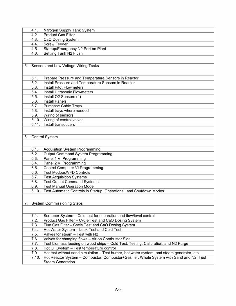
4.1. Nitrogen Supply Tank System 4.2. Product Gas Filter 4.3. CaO Dosing System 4.4. Screw Feeder 4.5. Startup/Emergency N2 Port on Plant 4.6. Settling Tank N2 Flush

5. Sensors and Low Voltage Wiring Tasks

5.1. Prepare Pressure and Temperature Sensors in Reactor 5.2. Install Pressure and Temperature Sensors in Reactor 5.3. Install Pitot Flowmeters 5.4. Install Ultrasonic Flowmeters 5.5. Install O2 Sensors (4) 5.6. Install Panels 5.7. Purchase Cable Trays 5.8. Install trays where needed 5.9. Wiring of sensors 5.10. Wiring of control valves 5.11. Install transducers

6. Control System

6.1. Acquisition System Programming 6.2. Output Command System Programming 6.3. Panel 1 VI Programming 6.4. Panel 2 VI Programming 6.5. Control Computer VI Programming 6.6. Test Modbus/VFD Controls 6.7. Test Acquisition Systems 6.8. Test Output Command Systems 6.9. Test Manual Operation Mode 6.10. Test Automatic Controls in Startup, Operational, and Shutdown Modes

7. System Commissioning Steps

7.1. Scrubber System – Cold test for separation and flow/level control 7.2. Product Gas Filter – Cycle Test and CaO Dosing System 7.3. Flue Gas Filter – Cycle Test and CaO Dosing System 7.4. Hot Water System – Leak Test and Cold Test 7.5. Valves for steam – Test with N2 7.6. Valves for changing flows – Air on Combustor Side 7.7. Test biomass feeding on wood chips – Cold Test, Testing, Calibration, and N2 Purge 7.8. Hot Oil System – Test temperature control 7.9. Hot test without sand circulation – Test burner, hot water system, and steam generator, etc. 7.10. Hot Reactor System – Combustor, Combustor+Gasifier, Whole System with Sand and N2, Test

Steam Generation

A-8

APPENDIX B: BCHP System Test Plan and Details of BCHP Plant Performance BCHP System Test Plan A number of test runs will be conducted with the pilot-scale BCHP system to collect data on the performance of the system. This test plan details the data collection during these tests. The performance of the BCHP system in conversion of the agricultural biomass feedstock to combustible gas for power production and heat utilization will be demonstrated relative to the efficiency and other performance objectives for this project.

The complete FICFB system is controlled by an advanced SCADA system that monitors the multiple components of the system during operation and controls the operation of the equipment using variable control valves and variable frequency drives. Figure 4.1 shows some views of the control room with the panel of drives that control all of the process equipment and the operator panels that show the SCADA interface used by the operator to monitor the process. There are a number of types of sensors used by this system including thermocouples, pressure transducers, gas and water flowmeters, electronic scale systems, level sensors, gas analyzers, and others. Several of these sensors are shown on the plant in Figure 4.2. The location of the sensors is included in the following section that describes the monitoring systems used during the test runs to monitor the performance of the BCHP system.

In order to monitor the process during the test runs on agricultural biomass, the data from the SCADA system which includes all of the sensors and all of the equipment set-points (valves and motor drives) was recorded on a continuous basis. The SCADA system monitors thermocouples, pressure transducers, oxygen sensors, flow meters, and ultrasonic level sensors at each subsystem. The SCADA system also controls pneumatic valves are used to set the flowrate of super-heat steam, air and compressed hot water of the system. A total of 18 variable frequency drives, which control the motors of the gasifier subsystems, are also integrated into the PLC-based SCADA system. The SCADA system architecture is shown in Figure 4.3 and a photo of the two PLC panels that are incorporated into the plant are shown in Figure 4.4. A total of 114 analog input channels, 10 analog output channels, and 8 digital input/output channels to monitor and control the whole gasification process via a National Instruments PLC control system. The PLC system is controlled by LabVIEW software, a graphical programing platform. Figure 4.5 shows the screen shoot of the gasifier front panel during a gas production operation period. During the operation of the plant, the SCADA system scans and displays the sensor readings on a 2-second interval and also records a time-stamped 30-second average of the scans.

The types of sensors utilized in the plant and recorded by the SCADA system are described in Table 4.1. The locations of the various sensors are shown in Figure 4.6 through Figure 4.12 with the label “T” showing locations of thermocouples, “P” showing locations of pressure transducers, “F” showing locations of flowmeters, and “L” showing the location of level

B-1

sensors. The manufacturer operating, maintenance, and calibration procedures were followed for these sensors.

The test runs will consist of a cold plant startup, operation with gas production from agricultural biomass, and a complete plant shutdown back to cold condition. A minimum of five multi-day test runs will be completed and all sensor data will be recorded by the SCADA system for the entire operating period. Post-processing of the data included calculating weighted averages over a time periods of stable operation to determine energy and mass balance relationships for all of the parameters detailed in the objectives.

Figure B.1: Motor Drive Systems (left) and SCADA Operator Interface (right) in BCHP Control Room

Figure B.2: Various Sensor Systems Utilized to Monitor and Control the BCHP Process

B-2

Figure B.3: SCADA System Architecture Based on PLC Input/Output Modules Connected to Operator Computer System

Figure B.4: SCADA System PLC Panels on the BCHP Plant

B-3

Figure B.5: SCADA System Front Panel

B-4

Table B.1: Sensors Used in SCADA System to Monitor the BCHP Operation and Performance

Sample/Measurement Method Location/Details

5 Gasifier temperature (°C)

10 Combustor temperature (°C)

12 Clean-up system temperature (°C)

25 Heat recovery system temperature (°C)

K-type thermocouple continuously monitored by LabView DAQ system

Various locations on gasifier

Various locations on combustor

Various locations on clean-up stream

Various locations on heat recovery system

Gasifier/Combustor pressure (mBar, gauge)

Reactor cross-bed DP (mBar, differential)

Filter housing DP (“WC, differential)

Scrubber DP (“WC, differential)

Hot water pressure (psig, gage)

Steam and hot air pressure (psia)

Gage pressure transducer, monitored by LabView DAQ system

Differential pressure transducer, monitored by LabView DAQ system

Differential pressure transducer, monitored by LabView DAQ system

Gage pressure transducer

Absolute pressure transducer

Various locations on gasifier and combustor sides

Locations above and below the bed on gasifier and combustor

Gasifier and Combustor filter housings’ inlet to filter housings’ outlet, DP

Scrubber inlet to scrubber outlet, DP

Recovery heat system hot water lines

Various locations on steam and hot air lines

B-5


Fluidizing air flow rate (kg/s)

Fluidizing steam flow rate (kg/s)

Flue gas flow rate (kg/s)

Syngas flow rate (kg/s)

Hot water flow rate (L min-1)

N2 flow rate (L min-1)

N2 flow rate (L min-1)

Steam make-up water flow rate (L min-1)

Pitot tube via DP transducers monitored by LabVIEW DAQ system

Ultrasonic flow meter

Mass flow meter

Anemometer

Vortex flow meter

Combustor air lines

Steam generator, Gasifier, & cyclone steam lines

Combustor flue gas line

Gasifier downstream line

Heat recovery line

Feeder screw box

Gasifier bag house

Water inlet of steam generator

Biodiesel level sensor (inch)

Condensate water level sensor (inch)

Ultrasonic level sensor connected to LabVIEW DAQ system

Scrubber settlement tank

Feedstock mass (kg/lb)

Floor scale monitored via RS232 to LabVIEW DAQ system

Feedstock weighed rea-time during operation

Gasifier/combustor oxygen sensor (%)

Back-up oxygen sensor (%)

Paramagnetic oxygen analyzer monitored by LabVIEW DAQ

Zirconia type oxygen analyzer

Locations on gasifier and combustor downstream lines

B-6


Gas composition (% by vol)

Gas composition (% by vol)

CH4, CO, CO2, C6H6, C7H8, C10H8 by on-line FTIR

H2, CH4, N2, CO, CO2, on-line or of grab samples by gas chromatography

Sampling after the clean-up system


Tar concentration and composition (g m-3, % by vol)

Tar concentration (g m-3, % by vol)

Gravimetric by BSI – 15439:2006 tar standard

SPA


B-7

Figure B.6: Locations of Sensors on FICFB Reactors

B-8

Figure B.7: Locations of Sensors on Heat Recovery System

Figure B.8: Locations of Sensors on Steam Generator System

B-9

Figure B.9: Locations of Sensors on Product Gas Filter System

Figure B.10: Locations of Sensors on Product Gas Scrubber System

B-10

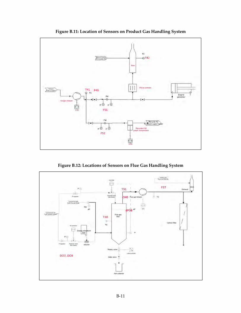
Figure B.11: Location of Sensors on Product Gas Handling System

Figure B.12: Locations of Sensors on Flue Gas Handling System

B-11

APPENDIX C: Technology Transfer Plan and Activities Technology Transfer Plan The purpose of this technology transfer plan is to share the BCHP technology and project progress and results with other technology experts, other researchers, and with the larger community and agricultural processing industry. There are three ways that the project team will do this: 1. Conference Presentations; 2. Annual Project Review Meetings; and 3. Technology Presentations to Community and Industry.

Conference Presentations:

The project team will attend technical conferences and present the status and results of the project with other subject matter technical experts in the area of thermochemical conversion of biomass for energy. These are national and international gatherings of experts in this field where knowledge can be transferred to others and help spread the technology and efforts of California to improve technology. These meetings are also a chance for the project team to keep informed on other efforts that may be beneficial and complementary to this project. The team will give at least two technical conference presentations per year during the course of the project.

Annual Project Review Meetings:

The project team will gather the entire project team, including remote and related project researchers, to review the project related results from each part of the technology development effort. The CEC project manager and the TAC will be invited to participate in these annual meetings. This is an opportunity to share results and transfer knowledge between the project participants and advisors and improve the technology results. These meetings will occur once per year in 2012, 2013, and 2014.

Technology Presentations to Community and Industry:

West Biofuels, with the support of UCSD, will give technology presentations to industry, government, and community members interested in the BCHP technology and agricultural applications. These presentations will take place at the project site and at other locations on an invited basis. These presentations are opportunities to transfer information about the project and BCHP technology to a wider audience. The team anticipates giving at least five of these presentations per year during the course of the project.

The proceeding section includes a listing of the relevant technology transfer presentations and meetings conducted to support the requirements of the Technology Transfer Plan.

C-1

Conference Presentations 2012

A. Bambal and R. Cattolica, ”Steam Reforming of Simulated Producer Gas Mixtures Containing Toluene, Ethylene, and Methane over Ni Catalyst,” AICHE 2012 Annual Meeting, Pittsburg, PA Oct. 28 – Nov. 2, 2012.

K. Mandich and R. Cattolica, “Computational Fluid Dynamics Study of Fluidized Bed,” 9th International Conference on CFD in Minerals and Materials Processing Conference, Melbourne, Australia, December 9 -12, 2012.

2013

D. Wise, R. Seiser, D. Olsen, and R. Cattolica, “Producer Gas and Natural Gas Performance in a CFR Engine,” 2013 Fall Technical Meeting Western States Sections of the Combustion, Colorado State University, Ocober 8-10, 2013, Fort Collins, Co.

Ashish Bambal, Reinhard Seiser, and Robert Cattolica, “Improved Tar Reforming in Producer Gas with Calcium Deposition on Gasifier Bed Materials,” TCBiomass 2013, International Conference and Thermochemical Conversion Science, sponsored by the US DOE, Chicago, Il, September 3-6, 2013.

C Liao, M. Summers, R, Seiser, C. Acharya, R. Cattolica and R. Herz, “Simulation of a Pilot-Scale Dual-Fluidized-Bed Gasifier for Biomass,” TC Biomass 2013, International Conference and Thermochemical Conversion Science, sponsored by the US DOE, Chicago, Il, September 3-6, 2013.

M. Summers, C. Liao, R, Seiser, R. Cattolica, R. Herz , and R. Rauch, “Biomass Combined Heat and Power in the Agricultural Processing Sector Using Fluidized Bed Gasification,” TC Biomass 2013, International Conference and Thermochemical Conversion Science, sponsored by the US DOE, Chicago, Il, September 3-6, 2013.

2014

Kevin J. Mandich and Robert J. Cattolica, “Bed expansion and pressure drop in a bubbling fluidized bed,” 10th International Conference on CFD in Oil & Gas, Metallurgical and Process Industries, SINTEF, Trondheim, Norway17-19 June 2014.

Reinhard Seiser, Ashish Bambel, Robert Cattolica and Bryan Jenkins, “Performance of Ni-based Catalyst for Tar and Producer-Gas Reforming,” TCS 2014, Symposium on Thermal and Catalytic Sciences for Biofuels and Biobased Products, sponsored by the US DOE, Denver, CO, September 2-5, 2014.

M. Summers, C. Liao, R, Seiser, R. Cattolica, R. Rauch, G. Faussone, “Biomass Combined Heat and Power in the Agricultural Processing Sector,” TCS 2014, Symposium on Thermal and Catalytic Sciences for Biofuels and Biobased Products, sponsored by the US DOE, Denver, CO, September 2-5, 2014.

C-2

Robert Cattolica, Reinhard Seiser, Hui Liu, Matthew Summers, and Peter Paul,” A Fast Circulating Fluidized Bed Gasification Pilot Plant for the Conversion of Biomass for Combined Heat and Power,”BioEnergy Australia 2014, Adelaide, Australia, Dec 1-4, 2014.

C-3

Annual Project Review Meetings UC Discovery/CIEE/CEC Program Review Meeting

UC San Diego – UC Berkeley – UC Davis

Thursday, October 18, 2012

UC Davis

Academic Surge, Room 2050

10:00 – 10:20 Introduction/Overview of Program Plan Robert Cattolica (UCSD)

10:20 – 10:50 Recent Gasifier Operational History/Performance Chang-hsien Liao (West Biofuels

10:50 – 11:20 Gasifier System Upgrade and Schedule Matt summers (West Biofuels)

11:20 – 11:40 UCD Gasifier Status R. Williams (UCD)

11:40 - 12:000 UCD Gasifer Gas Cleaning Systems Status Zach McCaffrey(UCD)

12:00 – 12:15 Review Material Analysis Systems (UC Davis /Woodland) Patrick Fitzgerald (UCD)

12:15 – 1:00 Lunch in Room 3102-B

1:00 – 1:30 Fluidization Modeling Status Kevin Mandich (UCSD)

1:30 – 2:00 Engine Research Status/Schedule Andrew Van Blarigan (UCB)

2:00 – 2:30 Almond Biomass Reseach Status Jenkins/Williams (UCD)

2:30 – 3:00 Reforming Catalyst Performance Status Ashish Bambel (UCSD)

3:00 – 3:30 Fixed Tar Reforming Experiment Status Reinhard Seiser (UCSD)

3:30 - 4:30 Discussion of Future Objectives for Investigators All

4:30 – 5:00 Transit to Steve’s Pizza in Woodland 4:30 – 5:00

5:00 – 6:30 Dinner 5:00 – 6:30

6:30 – 7:00 Transit to Sacramento Airport 6:30 – 7:00

C-4

UC Discovery/CIEE/CEC Program Review Meeting

UC San Diego – UC Berkeley – UC Davis – West Biofuels

Thursday, October 17, 2013

UC Davis

135 Everson Hall


10:20 – 10:50 Gasifier Operational History/Performance Chang-hsien Liao (West

Biofuels)

10:50 – 11:20 Gasifier System Upgrade and Schedule Matt Summers (West Biofuels)

11:20 – 11:40 UCD Gasifier Status Operations Jenkins/Williams (UCD)

11:40 - 12:00 UCD Gasifer Gas Cleaning Systems Results Zach McCaffrey (UCD)

12:00 – 12:40 Lunch

12:40 – 1:00 Fluidization Modeling Status Kevin Mandich (UCSD)

1:00 – 1:20 Aspen Modeling of Gasifier Systems Jesse Littlefield (UCSD)

1:20 – 1:40 Heat Transfer System Control Study Rich Herz (UCSD)

1:40 – 2:00 Reforming Catalyst Performance Status Tinku Biadya (UCSD)

2:00 – 2:20 Fixed Tar Reforming Experiment Status Reinhard Seiser (UCSD)

2:20 – 2:40 Break

2:40 – 3:00 Landfill Mining as an Energy Resource Yazdani/Seiser (UCD)

3:00 – 4:00 Tour of UC Davis Research Gasifier Michael Long (UCD)

4:00 -5:30 Tour of Woodland Biomass Research Center All

5:30 – 7:00 Dinner Steve’s Pizza in Woodland All

7:00 – 7:30 Transit to Sacramento Airport

C-5



Friday, October 18, 2013

UC Davis

1003 Kemper Hall


10:10 – 10:40 Producer Gas Combustion Kinetics Kal Seshadri (UCSD)

10:40 - 11:00 Rapid Compression Modeling of Producer Gas Kinetics Ulrich Niemann (UCSD)

11:00 – 11:30 Producer Gas CFR Lean Combustion/Emission Results Dan Olsen (CSU)

11:30 – 12:00 Producer Gas Methane Number Experiments/Model Dan Wise (CSU)

12:00 – 1:00 Lunch

1:00 – 1:30 3-way Catalyst CFR Engine Emission Reinhard Seiser (UCSD)

1:30 – 1:50 Lean Combustion SCR Emission Control Chris Weaver (EF&EE)

1:50 – 2:10 Combustion Emission Capture Chang-Yul Cha (Cha Corp)

2:10 – 4:00 Tour of Woodland Biomass Research Center All

C-6



Wednesday, December 17, 2014

UC Davis

1065 Kemper

12:00 – 1:00 Lunch

1:00– 10:15 Introduction/Overview/Future Program Plans Robert Cattolica (UCSD)

1:15– 1:45 Gasifier System Status – Future Program Plan Matt summers (West Biofuels)

1:45– 2:05 Gasifier Operational History/Performance Chang-hsien Liao (West Biofuels)

2:05 – 2:25 System Monitoring – Gasifier – Engine – Set up Reinhard Seiser (UCSD)

2:25 – 2:45 Aspen Modeling – Heat Recovery – Overall System Jesse Littlefield (UCSD)

2:45 – 3:00 Break

3:00 – 3:20 Advanced CFD simulation Hui Lui (UCSD)

3:20 - 3:40 Economic Analysis of 3MWe Power Production Cattolica/Emmenegger (UCSD)

3:40 – 4:00 Fixed-bed Tar Reforming Experiment Status Reinhard Seiser (UCSD)

4:00 – 4:15 UCD Fluidization Reactor Status Michael Long/Jenkins (UCD)

4:15 - 5:00 Tour UCD Fluidization Reactor Michael Long

5:30 - 6:30 Tour of Woodland Biomass Research Center All

6:30 - 7:30 Dinner Steve’s Pizza in Woodland All

C-7

Technology Presentations to Community and Industry

Date Participating Organizations Location

7/18-7/20/2012 GREG, Consulectra, Vienna Technical University Vienna, AT

7/23-7/28/2012 Biomass Kraftwerk Gussing, EEE Gussing, AT

11/8/2012 J.G. Boswell Farms, WAPA Remote Meeting

12/14/2012 UC Workshop: Community-Scale Energy from Biomass

Davis, CA

1/16/2013 GREA, GREG, Ainsworth Energy Woodland, CA

1/28/2013 TSS Consultants Sacramento, CA

2/7/2013 J.G. Boswell Farms Woodland, CA

6/6/2013 California Department of Food and Agriculture Sacramento, CA

7/2/2013 CEC Staff Integrated Energy Policy Report Workshop

Sacramento, CA

9/25/2013 WAPA Workshop Fresno, CA

10/16/2013 Southern California Gas, Burns & McDonnell Woodland, CA

11/6/2013 City of Burlington Burlington, VT

1/30/2014 Caterpillar, Inc., Holt of CA Woodland, CA

8/19/2014 Pivotal IRM Woodland, CA

9/22/2014 AG TEC, WAPA, San Joaquin Valley APCD Fresno, CA

10/7/2014 Southern California Gas, Burns & McDonnell Woodland, CA

10/17/2014 Central Valley Ag Processors Kerman, CA

11/12/2014 Ag Energy Consumers Association, WAPA Workshop

Fresno, CA

12/17/2014 SMUD Woodland, CA

3/5/2015 Mendocino Forest Products Ukiah, CA

C-8

demonstrati on of advanced biomass …€¦ · · 2016-05-02final project report . demonstrati on...

Documents