demonstration of optimisation of plumbosolvency treatment...

DWI 6173 AUGUST 2003

Demonstration of Optimisation of Plumbosolvency Treatment and Control Measures

Final Report to the Drinking Water Inspectorate

DEMONSTRATION OF OPTIMISATION OF PLUMBOSOLVENCY TREATMENT AND CONTROL MEASURES

Final Report to the Drinking Water Inspectorate

Report No: DWI 6173

Date: August 2003

Authors: P J Jackson and J C Ellis

Contract Manager: P J Jackson

Contract No: 13398-0

DWI Reference No: DWI 70/2/178

Contract Duration: January – March 2003

Any enquiries relating to this report should be referred to the Contract Manager at the following address: WRc-NSF Ltd, Henley Road, Medmenham, Marlow, Buckinghamshire SL7 2HD. Telephone: + 44 (0) 1491 636500 Fax: + 44 (0) 1491 636501

This report has the following distribution: Internal: Authors

i

CONTENTS Page

LIST OF TABLES II

LIST OF FIGURES II

EXECUTIVE SUMMARY 1

1. INTRODUCTION 3 1.1 Background 3 1.2 Objectives 5 1.3 Layout of this report 5

2. MONITORING STRATEGIES 7 2.1 Methodology 7 2.2 Results 7

3. ASSESSMENT OF MONITORING STRATEGIES 13 3.1 Type of sample for lead analysis 13 3.2 Number of sampling points and frequency of monitoring 14 3.3 Other monitored parameters 15 3.4 Arrangements and methods for reviewing monitoring data 15 3.5 Lead pipe rigs 16 3.6 Orthophosphate monitoring at water treatment works 16

4. RECOMMENDATIONS 17 4.1 Monitoring strategies 17 4.2 Related issues 18 4.3 Statistical assessment of lead monitoring data 18

5. DISCUSSION 27

6. TOPICS FOR FURTHER REVIEW 29

Page

ii

APPENDICES

APPENDIX A WATER COMPANY MONITORING ARRANGEMENTS 31

APPENDIX B PIPE RIG TECHNICAL DATA 49

LIST OF TABLES

Table 2.1 Summary of monitoring arrangements 8 Table 2.2 Summary of lead monitoring methods 10 Table 2.3 Summary of approaches used 11 Table 2.4 Summary of data review and assessment arrangements 11 Table 3.1 Advantages and disadvantages of different sample types 13

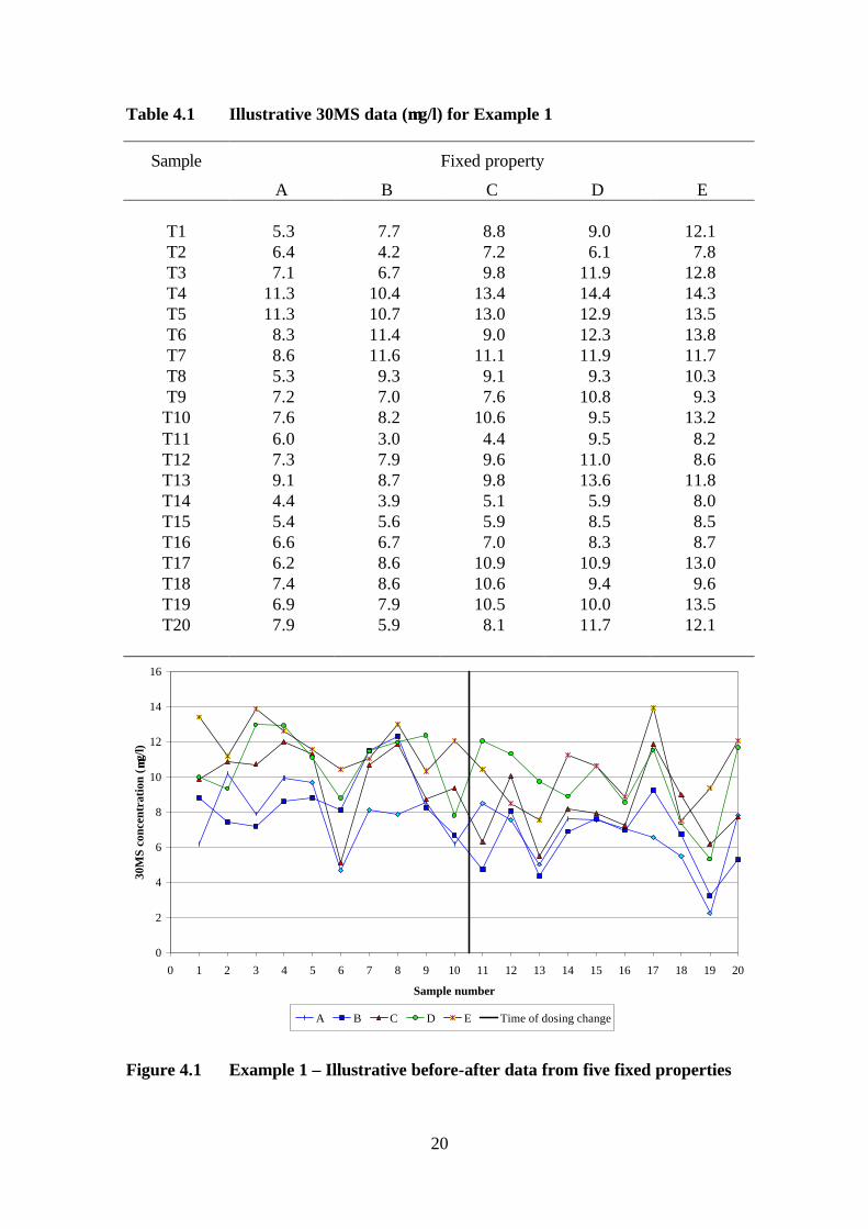
Table 4.1 Illustrative 30MS data (µg/l) for Example 1 20 Table 4.2 Outcome of t-tests on the Example 1 data (concentrations in

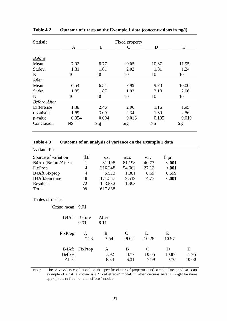
µg/l) 21 Table 4.3 Outcome of an analysis of variance on the Example 1 data 21 Table 4.4 Planning calculations for Example 1 22

LIST OF FIGURES

Figure 4.1 Example 1 – Illustrative before-after data from five fixed properties 20

Figure 4.2 Example 2 – Illustrative before-after RDT data for a supply zone 24

Figure 4.3 Outcome of Fisher's Exact Test for various choices of threshold 25 Figure 4.4 Illustrative statistical power curves for the Mann-Whitney test 26

1

EXECUTIVE SUMMARY

The 1998 Drinking Water Directive specifies an interim Parametric Value (PV) for lead at consumers’ taps of 25 µg/l (to be met by 25 December 2003) and a final PV of 10 µg/l (to be met by 25 December 2013). These requirements are given effect by the Water Supply (Water Quality) Regulations 2000 and the Water Supply (Water Quality) Regulations 2001 for England and Wales respectively. The Drinking Water Inspectorate (DWI) has put in place Regulatory Programmes of Work for plumbosolvency treatment and control measures (usually, dosing orthophosphate) with a requirement to optimise these treatment measures. The objective of optimisation is to determine the orthophosphate dose (and other conditions) required to meet consistently the lead standard – i.e. to determine the treatment conditions required to obtain the best practicable and consistent reduction in lead concentrations.

A key element of optimisation is demonstration of the effectiveness of the measures taken. The type of sample taken from properties in distribution to assess lead levels following the introduction or modification of treatment varies between water companies. The most commonly used sample types are random daytime (RDT) and stagnation samples taken from a fixed set of properties within distribution. As a general rule, the results of fixed-point sampling are less variable than RDT sampling because the stagnation time is controlled. An alternative, or complementary, approach is the use of lead pipe rigs located at the water treatment plant or at convenient points within distribution (e.g. service reservoirs).

The objectives of this project are to review, analyse and report to DWI on water company arrangements and plans for monitoring plumbosolvency treatment and control at treatment works and in distribution.

Information on each company’s monitoring strategy was obtained principally by reference to DWI hardcopy and computer files including water company strategies for plumbosolvency treatment and control measures, DWI 2001 and 2002 Technical Audit inspection reports and completed proformas that were distributed to companies in advance of the 2002 Technical Audit. Additional information was obtained where necessary by e-mail correspondence with DWI’s company contact. The information was summarised in terms of numbers of sampling locations of each type for each treatment scheme, the frequency of monitoring, parameters monitored in addition to lead and arrangements for monitoring the concentration of orthophosphate dosed. The use and operation of pipe rigs were reviewed. Information was also obtained and summarised on the frequency with which monitoring data are reviewed and what statistical techniques are used to assess the results.

Recommendations are made on monitoring strategies in terms of sample type, numbers of sampling points, sampling frequency and so on. Suggestions are also made on related issues, such as monitoring of orthophosphate dose. Examples are given of statistical methods for assessing lead monitoring data, including planning the number of samples required. Topics that merit further review are identified.

3

1. INTRODUCTION

1.1 Background

The 1998 Drinking Water Directive specifies an interim Parametric Value (PV) for lead at consumers’ taps of 25 µg/l (to be met by 25 December 2003) and a final PV of 10 µg/l (to be met by 25 December 2013). These requirements are given effect by the Water Supply (Water Quality) Regulations 2000 and the Water Supply (Water Quality) Regulations 2001 for England and Wales respectively. The Drinking Water Inspectorate (DWI) has put in place Regulatory Programmes of Work (RPoW) for plumbosolvency treatment and control measures. These have varying dates for completion of feasibility study and investigations and design, installation and commissioning of appropriate treatment solutions to reflect particular water company needs and phasing of overall construction programmes. They also include a requirement to optimise these treatment measures by 25 December 2003. The process for meeting the new standards for lead as set down in the RPoW comprises assessment and justification of the need for the following stages:

– installation of treatment to reduce plumbosolvency; – optimisation of plumbosolvency treatment measures; – opportunistic lead pipe replacement; – strategic pipe replacement to meet 25 µg/l; and – strategic pipe replacement to meet 10 µg/l.

In England and Wales, treatment to reduce plumbosolvency generally consists of dosing orthophosphoric acid or a sodium orthophosphate to achieve a target concentration that is usually in the range 1 to 2 mg/l as P. The pH may also be adjusted although the effectiveness of orthophosphate is relatively insensitive to pH. Increasing the orthophosphate concentration reduces the solubility of lead but the additional benefits of increasing the dose diminish as the dose is increased. Thus, there are optimum conditions of orthophosphate dose (and other variables such as pH) to achieve a target value for the lead concentration at the tap.

The objective of optimisation is to determine the orthophosphate dose (and other conditions) required to meet consistently the lead standard – i.e. to determine the treatment conditions required to obtain the best practicable and consistent reduction in lead concentrations. It should be noted that the “optimum dose” may vary with time and according to circumstances (e.g. water quality).

Once optimum conditions have been established, it is clearly important that the orthophosphate dose is controlled and maintained at the optimum. Orthophosphate monitoring and dose control practices vary substantially within the water industry.

4

The RPoW require each water company to have and to implement a plumbosolvency treatment and control strategy. DWI Information Letter IL 3/2001 contains a model framework for such a strategy that includes:

– data requirements; – identification of treatment works requiring plumbosolvency treatment and control

(and optimisation of existing and new treatment); – deciding when treatment is beneficial (i.e. a significant reduction in lead

concentrations); – optimisation of treatment and control; – monitoring and control at treatment works; – monitoring and control in distribution; and – timescales.

Water company strategies have been submitted to DWI and are generally satisfactory in identifying and justifying the content of the RPoW, i.e. when and where treatment would be beneficial, and for the installation and commissioning of plant. A key element is the requirement for water companies undertaking plumbosolvency control measures to demonstrate the effectiveness of the measures taken. The type of sample taken from properties in distribution to assess lead levels following the introduction or modification of treatment varies between water companies. The most commonly used sample types are random daytime (RDT) and fixed stagnation time samples, typically 30 minutes stagnation (30MS). An alternative, or complementary, approach is the use of lead pipe rigs located at the water treatment plant or at convenient points within distribution (e.g. service reservoirs).

The strategy provided in IL 3/2001 for demonstrating the effectiveness and optimisation of treatment in distribution is 30MS sampling from the same property taken three times per week each month. A small number of locations (properties) in each scheme (area of supply) should be sampled before treatment, after introduction of treatment and following each relevant change in treatment. Only leaded properties should be sampled. Lead pipe rigs sited at appropriate points within the distribution system are an acceptable alternative.

As a general rule, the results of 30MS sampling are less variable than RDT sampling because the stagnation time is controlled. Therefore fewer 30MS samples should be needed to achieve the same statistical precision and confidence compared to RDT sampling. There are, however, a number of practical issues that have to be considered by water companies when setting up monitoring systems. RDT sampling is more acceptable to consumers than 30MS sampling. It may be difficult to obtain co-operation from consumers to allow regular sampling over the prolonged period needed to demonstrate that treatment continues to be optimised. Therefore, in terms of practicality and sustainability, strategically located pipe rigs may be preferable to sampling at consumers’ taps.

Some water companies have included optimisation of treatment and monitoring and control at treatment works and in distribution in their strategies and, where appropriate, these have been agreed with DWI. However, most water companies do not have the optimisation and monitoring/control elements of their strategies agreed with DWI and

5

these need to be developed. Some water companies have adopted different monitoring strategies to that proposed in IL 3/2001.

DWI has agreed with the national Lead Working Group that existing strategies should be developed on a modular basis, and is preparing an Information Letter to provide further guidance to water companies on the development and updating of existing strategies to provide detailed optimisation details. In the meantime, DWI has awarded a contract to WRc-NSF to conduct research work to inform its continuing advice to water companies. The main area of this research concerns the monitoring carried out by water companies for optimisation of plumbosolvency treatment and control arrangements.

1.2 Objectives

The overall objectives of the contract are to review, analyse and report to DWI on water company arrangements and plans for monitoring plumbosolvency treatment and control at treatment works and in distribution:

(a) to demonstrate optimisation of plumbosolvency treatment and control measures;

(b) to maintain optimised conditions at treatment works and in distribution;

(c) to advise on good practice in achieving optimised conditions, and in maintaining optimised conditions;

(d) including an assessment of the appropriateness of the sampling undertaken, and advice on good practice for the principal sampling methodologies employed by water companies; and

(e) including an assessment of the current use of lead pipe rigs for plumbosolvency monitoring, an assessment of the compatibility of different models of lead pipe rigs in current use, and advice on good practice in lead pipe rig use in this context.

1.3 Layout of this report

Section 2 summarises the monitoring strategy adopted by each water company.

Section 3 provides an assessment of the strategies that are summarised in Section 2.

Section 4 provides recommendations regarding monitoring strategies.

Section 5 discusses the key findings and observations.

Section 6 identifies topics for further review.

Appendix A provides details of each company’s approach to monitoring.

Appendix B provides technical information on commercially available and in-house built lead pipe rigs.

7

2. MONITORING STRATEGIES

2.1 Methodology

The information on each company’s monitoring strategy was obtained principally by reference to DWI hardcopy and computer files:

• water company strategies for plumbosolvency treatment and control measures;

• DWI 2001 and 2002 Technical Audit inspection reports; and

• completed proformas that were distributed to companies in advance of the 2002 Technical Audit.

Additional information was obtained where necessary by e-mail correspondence with DWI’s company contact.

2.2 Results

In this report the water companies have been assigned code letters from A to W inclusive. Each company’s monitoring strategy is described in Appendix A. Table 2.1 provides a summary of the arrangements for monitoring lead and other parameters, and monitoring orthophosphate concentrations at treatment works. In Table 2.1 the following terminology is used:

RDT Random Daytime Samples – either regulatory compliance samples or “special” samples taken for optimisation monitoring (see below).

FIXED Stagnation samples taken from a set of fixed lead-plumbed properties in distribution. These are 30 minutes stagnation samples (30MS) unless otherwise indicated.

RIG Stagnation samples taken from lead pipe rigs located within distribution. These are 30MS samples unless otherwise indicated.

Blank entries in Table 2.1 for “Number per scheme” and “Sampling frequency” indicate that the company is not using that type of sample for monitoring the optimisation of plumbosolvency treatment.

All water companies have to take regulatory compliance RDT samples for lead, irrespective of lead treatment optimisation monitoring. However, some companies have elected to use compliance samples as part of their optimisation monitoring – these are indicated as “Compliance” in the Number per scheme entry for RDT samples in Table 2.1. Other companies are using RDT sampling at an enhanced frequency for optimisation – indicated by “Enhanced” in Table 2.1.

8

Table 2.1 Summary of monitoring arrangements

Number per scheme Sampling frequency Other parameters P monitoring Code RDT FIXED RIG RDT FIXED RIG

A 4-9 (60MS) Monthly pH, P, Cond On-line B Enhanced 84-420/y pH, P, T Grab daily C Compliance 1-3 1 Monthly Weekly Weekly pH, P, Alk, T On-line + weekly

grab D Enhanced 1-9 100-1700/y pH, P, Alk, T Some on-line, weekly

grab E ? 3 (60MS) 2/week 2/week ? ? F Enhanced 2-5 100/y Weekly P, pH, Alk, T On-line + daily-

weekly grab G Enhanced 1-2 25/y 1-2/week P, Alk, T (RDT only) Weekly grab H 1-4 1-4/month pH, P, Alk, T, Turb Grab daily I Enhanced 1-4 (60MS) 52-132/y 4/month

(clusters) pH, P Weekly grab

J Enhanced <=30 Total 19 >1/week Weekly Weekly pH, P, T, Turb Grab weekly K 2-4 1-2 Monthly Monthly pH, P, Alk, T, Col On-line + daily-

weekly grab L Enhanced 520/y P, T On-line M Enhanced 12-648/y pH, P, Cond, Fe, T Grab daily N Enhanced 2 50/zone/y Weekly pH, P (rig Alk, Col,

T) Grab weekly

9

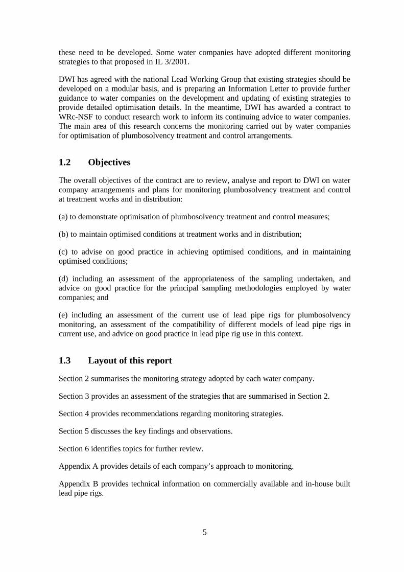
Table 2.1 Continued

Number per scheme Sampling frequency Other parameters P monitoring Code RDT FIXED RIG RDT FIXED RIG

O Compliance 2 or 3 Compliance Weekly pH, P, Alk, T On-line + daily grab P 1-7 (8H) Weekly P, T On-line Q 1-9 1-4 3/month

(clusters) 3/week (clusters)

pH, P, Alk, T, RDT, FF, 30MS

Grab 3-5/week

R Compliance 2-10 1 Compliance 3/month ? P, T On-line + daily-weekly grab

S Enhanced Total 25 8/zone/month Weekly pH, P, Alk, TOC, Fe Some on-line, weekly grab

T Compliance 4-12 1 or 10 Compliance Monthly Weekly pH, P, T, RDT, FF Grab 2/week U Compliance 1-3 Compliance Weekly pH, P, T On-line + weekly

grab V Compliance 1-5 1-3 Compliance Monthly Weekly pH, P, T, (RDT, FF,

30MS) Grab daily

W 1-14 (8H) 1-6 3/3 months (clusters)

Weekly pH, P, Alk, DOC On-line + daily-weekly grab

P = orthophosphate Alk = alkalinity T = temperature TOC/DOC = Total/Dissolved Organic Carbon FF = fully flushed lead

10

In Table 2.1 “Other parameters” indicates the other determinands measured in conjunction with sampling for lead. In some cases when sampling from fixed properties or rigs a sequence of samples is taken – RDT, fully flushed (FF), 30MS. These samples are included under “Other parameters”.

Orthophosphate concentrations are checked at the treatment works by either or both on-line monitors or by analysis of grab samples, as indicated in Table 2.1.

It is clear from Table 2.1 that various sample types and combinations thereof are being used by different companies. Table 2.2 summarises the lead monitoring methods employed by each company and Table 2.3 indicates the number of companies that are using each of the possible approaches. Most companies are using a combination of different types of sample for monitoring optimisation.

Table 2.4 summarises each company’s arrangements for formally reviewing the monitoring data and the methods of assessment in use or proposed.

Table 2.2 Summary of lead monitoring methods

Code Monitoring method(s)

A FIXED B FIXED + RIG C RDT + FIXED + RIG D RDT + RIG E RDT + RIG F FIXED G RDT + RIG H FIXED + RIG I RDT J RDT + FIXED + RIG K RDT + FIXED L RIG M RDT + FIXED + RIG N RDT + RIG O RDT + RIG P RIG Q RDT + RIG R RDT S RDT T RDT + FIXED + RIG U RDT + RIG V RDT + RIG W FIXED + RIG

11

Table 2.3 Summary of approaches used

Approach Number of companies

RDT 3 FIXED 2 RIG 2 RDT + FIXED 1 RDT + RIG 8 FIXED + RIG 3 RDT + FIXED + RIG 4

Table 2.4 Summary of data review and assessment arrangements

Code Data review Assessment of data

A 4-6 weeks Graphical B As necessary >10 µg/l, t test, Welsh's C ? Graphical D Monthly >10 and 25 µg/l, E ? ? F Weekly/Monthly/Quarterly Non linear regression/ Mann Whitney

Wilcoxon/summary G ? ? H ? ? I Monthly Graphical J ? None K Quarterly Graphical L Quarterly Summary, >10 and 25 µg/l, M Monthly Control charts, Fisher Exact N Monthly/weekly Mann-Whitney U O Monthly Graphical P Continuous Graphical Q 2 months Statistical assessment not performed to date R ? Summary statistics S Weekly/Monthly/Quarterly Control charts (various) T Quarterly Tabulate, %reduction, RDT >25 and 10 µg/l, U Monthly Graphical V Continuous Graphical W Monthly >10 µg/l

13

3. ASSESSMENT OF MONITORING STRATEGIES

3.1 Type of sample for lead analysis

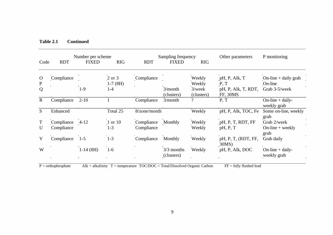
For the purpose of this report the only types of sample considered are RDT, FIXED and RIG as defined in Section 2. Their relative advantages and disadvantages are summarised in Table 3.1.

Table 3.1 Advantages and disadvantages of different sample types

Sample type Advantages Disadvantages

RDT Simple, inexpensive and quick to

collect Acceptable to consumers Results will indicate %compliance

Less reproducible than FIXED If truly random, will include non-leaded properties

FIXED More reproducible than RDT Time consuming and relatively

expensive to collect Inconvenient to consumers

RIG More reproducible than RDT

No inconvenience to consumers Automated sampling

May not reflect actual values of lead concentrations at properties

In principle any or all of these sample types could be used to demonstrate optimisation of plumbosolvency treatment and the choice between them is likely to be based on practicality and individual company preference.

There is a long history of using RDT sampling for compliance monitoring. Using RDT sampling has the advantage that the results should also indicate the extent of compliance. RDT sampling is simple, inexpensive and more acceptable to consumers than stagnation sampling. However, because stagnation time is uncontrolled the results of RDT sampling are far less reproducible than those of fixed stagnation time sampling. Consequently many more samples are needed to give the same amount of information as fixed stagnation time samples1.

1 It is not possible to quantify how many more samples would be needed since this will depend on the variability associated with each sample type, which may vary from location to location.

14

RDT samples (taken from random properties) will include a proportion of non-leaded properties. As a consequence the effects of changes to orthophosphate dose may be masked by the results from non-leaded properties whose lead concentrations are expected to be low and not affected by changes to dosing. Overall, therefore, it may prove more difficult to demonstrate optimisation using RDT sampling.

On the other hand, RDT sampling is much more practical than fixed-point stagnation sampling. It can take considerable effort to find consumers who are willing to co-operate, even when financial inducements are offered. Even when consumers can be persuaded to co-operate, they may become resistant to repeated visits and the drop-out rate can be quite high. If a property drops out before the conclusion of the monitoring programme, all of the data collected for that property becomes essentially valueless. Therefore, if it is planned to use fixed-point sampling, it may be necessary to secure a relatively large number of fixed properties at the beginning of the monitoring programme in anticipation of an assumed drop out rate. In the case of small schemes it may be difficult to find sufficient fixed points. A further difficulty with fixed-point sampling is ensuring that the chosen lead-plumbed properties give lead concentrations typical of lead-plumbed properties generally.

Lead pipe rigs avoid the disadvantages of both RDT and fixed-point sampling. Rigs fitted with new lead pipe will allow the effects of treatment and optimisation to be established. However, the absolute values for lead concentrations from pipe rigs may not be directly comparable with those from properties (and hence the results cannot be used directly to forecast the likely extent of compliance).

A monitoring programme should preferably include more than one type of sample in order to provide greater flexibility of response. For example, a reduction in the proportion of high lead concentrations is best demonstrated by RDT samples, whereas a decrease in mean concentration is shown most effectively by FIXED or RIG samples. Over 70% of companies are using more than one sample type and four of them are using all three sample types.

A small number of companies that are using fixed-point sampling rely on the customers to take the stagnation samples which are then collected on a “milk round” basis. If this practice is followed there is a risk that the consumer may not follow the correct procedure.

Some companies use 8-hour stagnation samples from fixed properties or rigs, rather than the more usual 30MS or 60MS. This is done presumably in order to generate higher lead concentrations and consequently to determine more easily whether changes have occurred. Eight-hour stagnation is atypical of normal domestic water usage patterns and it would be desirable for the trends in the results of 8-hour stagnation samples to be checked against another type of sample, e.g. RDT.

3.2 Number of sampling points and frequency of monitoring

The number of fixed sampling points and lead pipe rigs in distribution varies quite widely both between companies and between schemes within a company. In some cases

15

the numbers of fixed points and rigs appear to be insufficient for the effects of changes to treatment to be assessed statistically with a reasonable level of confidence. The number of sampling points required will depend on several factors including the size and complexity of the distribution system and the variability in lead concentrations between properties (or rigs). Some general guidance is given in Section 4.1.

For RDT sampling, the regulatory frequency2 is unlikely to be sufficient for statistical purposes (see Section 4.3). Some companies are sampling at an enhanced frequency but others are taking an inadequate number of samples.

For fixed properties and rigs, most companies sample weekly or three times per month, which should provide a sufficient number of “before” and “after” samples for statistical purposes within the typical timescale for optimisation. However, a few companies sample monthly, which is likely provide too few samples within a typical timescale for optimisation. Statistical power calculations can be used to determine the numbers of samples required, and hence the sampling frequency within a given period (see Section 4.3).

Few companies appear to have taken account of seasonal factors such as water temperature that will affect lead concentrations. If, for example, an increase in orthophosphate dose coincides with an increase in temperature, the temperature rise may mask the effect of the dose increase. Conversely, a decrease in temperature could exaggerate the effects of a change in treatment on lead concentrations. The external air temperature and the temperature within houses (or rig locations) may also affect lead concentrations. Other factors that impact on lead concentrations may also vary seasonally, for example organics content and alkalinity.

3.3 Other monitored parameters

Most companies are monitoring an adequate range of other determinands. The minimum test battery in addition to lead should be temperature, orthophosphate and pH (pH could be omitted for hard waters with very stable pH).

Other parameters that might be relevant in particular cases are discussed in Section 4.2.

A few companies take RDT and fully flushed (FF) samples from fixed properties in addition to 30MS samples. The purpose of this is unclear and the value of these additional samples – especially FF – is questionable.

3.4 Arrangements and methods for reviewing monitoring data

The frequency for reviewing the monitoring data varies between companies from “continuous” to quarterly. Simple scrutiny of data (e.g. graphical assessment) at a

2 Up to 4 samples per zone per year, or up to 24 if failures of the current 50 µg/l standard occurred in the previous year.

16

reasonable frequency gives early warning of outliers and potential data handling problems as well as giving an indication of trends in lead concentrations. Reviewing on a quarterly basis may be too infrequent, especially where sampling is carried out weekly. In several cases it is unclear what use is made of the results for other monitored parameters.

Most companies are not (yet) performing statistical analysis on the monitoring data and are relying on visual assessment of graphical information, although a few companies do have defined statistical methodology in place. Some companies assess the results against 10 and 25 µg/l target concentrations. Simple graphical treatment of the data is inadequate for assessing the effects (if any) of a change in treatment. Statistical assessment of the data should be performed once a sufficient amount of data has been accumulated. Suggested statistical approaches are given in Section 4.3.

3.5 Lead pipe rigs

Several different models of automatic lead pipe rigs are in use – see Appendix B. With few exceptions no systematic comparisons have been made between the results obtained with different models. This is particularly surprising since several companies use more than one model. Different rigs may give different changes in lead concentrations during optimisation and therefore it would be desirable for companies to check whether different models of rig give equivalent results.

The mode of operation of rigs varies; some companies operate them on a continuous cycle whilst others operate e.g. 16 hours on, 8 hours off. The period of flushing prior to initiating the 30 minutes stagnation varies significantly between companies. Such practical aspects of rig operation should be the subject of further review.

3.6 Orthophosphate monitoring at water treatment works

On-line orthophosphate monitors are installed at many water treatment works but at others reliance is placed on the analysis of grab samples, in some cases only sampled weekly. Several DWI Technical Audit reports identify substantial discrepancies between target and measured orthophosphate concentrations. It is necessary to confirm that the target dose is being applied consistently and infrequent grab sampling is likely to be inadequate for this purpose. One method for achieving consistent dosing is to install continuous orthophosphate monitors with feedback control of the dosing rate to achieve the set-point orthophosphate concentration. A decision on whether to install on-line orthophosphate monitoring needs to be considered on a case by case basis taking account of works manning, reliability and performance and the maintenance requirements of the monitor.

A further issue is the lack of agreement between results obtained using monitors, laboratory analysis and test kits identified in some Technical Audit reports. Where the results do not tally, there is a need to identify the cause of the disagreement and rectify it. However, determining an accurate value for the orthophosphate concentration is of secondary importance to ensuring that a consistent dose is applied.

17

4. RECOMMENDATIONS

4.1 Monitoring strategies

The choice of sample type (RDT, FIXED or RIG) is likely to be dictated by water company preference and practical considerations. Any of these sample types can be used to monitor and demonstrate optimisation provided that sufficient samples are taken from an adequate number of sampling points. It would be desirable to use more than one type of sample – as most companies are doing – to give greater assurance in the interpretation of the results.

In the few cases where customers undertake sampling, some duplicate sampling by a professional sampler is desirable to verify that the samples are being taken correctly. In addition it would be desirable to scrutinise the results from these samples to identify any “rogue” values.

In the few cases where 8-hour stagnation samples are taken from properties or rigs, the trends in the results should be verified against those for other sample types (e.g. RDT). This is because the chemistry of lead corrosion and dissolution may change with prolonged stagnation, as reactant and product concentrations change.

In the case of fixed properties and pipe rigs it is not possible to give definitive guidance on the number of sampling points required. Fewer sampling points could be used in small supply zones with consistent water quality compared to larger zones where water quality varies or which are fed from more than one works. Because water quality can vary within the distribution system, and because it should not be assumed that properties in a small part of the system are representative of the whole water supply area, sampling points should be spread across the distribution system. As a general guide the monitoring should include one or more points near the treatment works, one or more in the middle of the distribution system, and one or more at the extremities of the system. This approach will facilitate the monitoring of the penetration of the applied orthophosphate dose within distribution. However, it is recognised that it may prove difficult to obtain the preferred number and mix of sampling points in some cases, e.g. zones serving small populations. Local knowledge of, for example, the geographical distribution of lead-plumbed properties should be taken into account when selecting fixed properties for monitoring.

The number of samples required before and after a change to treatment can be calculated using methods such as those illustrated in Section 4.3. Given the anticipated duration of monitoring before and after a change in treatment, the required sampling frequency can then be calculated. With typical timescales for completion of stabilisation, monthly sampling from fixed properties and pipe rigs will not generate an adequate number of data points – weekly sampling would be more appropriate. Similarly, RDT sampling at the regulatory frequency will not provide a sufficient number of samples and the sampling frequency should be increased.

18

Seasonality effects need to be taken into account in interpreting changes in lead concentrations. If practicable, changes to dosing should be timed so that the “before” and “after” data span similar ranges of water temperature. However, it is recognised that this may not always be feasible in practice.

In addition to monitoring for lead, orthophosphate and temperature should always be measured. The pH should also be measured unless experience has shown that pH does not vary seasonally or within distribution. Other parameters that should be monitored in particular circumstances include:

• Alkalinity – in soft waters whose alkalinity is likely to vary seasonally.

• Iron and/or turbidity – where “dirty water” could be an issue and could impair the effectiveness of plumbosolvency treatment.

• Colour or TOC – in supplies derived from peaty sources, where the presence of natural organics could lead to an increase in lead solubility.

4.2 Related issues

Water companies should have formal arrangements for reviewing the lead monitoring data. This should be done on a monthly basis.

In addition to time-series plots of lead concentrations and other monitored parameters, statistical tools should be used to assess the monitoring data.

The results from lead pipe rigs should be assessed in relation to the results from either or both RDT samples and stagnation samples from fixed properties to determine any useful associations. It would also be desirable to compare the results from different models of rig installed in the same water supply zone. This would enable a more direct prediction of likely compliance based upon pipe rig data. Steps need to be taken to ensure that pipe rigs are sited away from sources of vibration that could give rise to erratic results. Lead pipe rigs should be set up with a sufficient flushing time prior to the stagnation period to ensure that all previously stagnated water is flushed from the system.

The use of on-line orthophosphate analysers to adjust the dosing rate automatically to achieve the set point should be considered on a case by case basis. If grab samples are used as the sole means of verifying the orthophosphate dose, they should be taken at a sufficient frequency to ensure that the target dose is met consistently.

4.3 Statistical assessment of lead monitoring data

4.3.1 Introduction

The main aim of the following examples is to outline simple ways in which the two main types of data might in principle be analysed. Of course, the statistical treatment will often need to be extended to accommodate the various complications that can arise in practice.

19

We briefly indicate some of these issues below. However, a more comprehensive treatment of these issues is most appropriately left until the next phase of the project.

4.3.2 Example 1 - Fixed properties (and pipe rigs)

The data

Suppose that five suitable properties are available, and that ten 30MS samples are taken at weekly intervals3 from each property before a change in dosing. After a suitable time has elapsed to allow stabilisation to occur, a further ten weekly samples are taken from each property.

The resulting data is shown in Table 4.1 and plotted in Figure 4.1. The example has been constructed so that half of the variation through time is common to all properties (e.g. due to seasonality or works-related factors), and half is due to random within-house variation and analytical error.

The analysis

One simple way to analyse the data is to carry out a independent-samples t-test on the ‘before’ and ‘after’ means for each property. This requires the within-house variability to be at least approximately Normally distributed – an assumption which is reasonable in this example. The results are shown in Table 4.2.

A more powerful way of analysing the data is to carry out a single analysis of variance (ANoVA) on the whole data set. This has two benefits. First, the temporal effect is estimated along with the ‘before’ and ‘after’ means for each property. This reduces the within-house variability and so improves the statistical power of the analysis. Secondly, the analysis will indicate whether the before-after effect is consistent across all five properties, or whether there is a statistically significant difference between properties. This provides useful information to help judge how representative the fixed properties are of reductions in lead concentrations generally across the supply zone.

The outcome of such an ANoVA in the present example is shown in Table 4.3. This shows that the overall before-after effect is significant at the p<0.001 level – which means that the effect is much stronger than when separate analyses were performed for each fixed property. The analysis also shows that there is no detectable difference in the size of the effect between properties.

3 In this simple example we assume that all five properties are sampled on the same day each week. In practice the sampling schedule is unlikely to be perfectly regular, and samples may be a few days apart. This is quite acceptable, and will scarcely weaken the analysis as long as the variations from week to week at a property tend to be larger than the within-week variation.

20

Table 4.1 Illustrative 30MS data (µµg/l) for Example 1

Sample Fixed property

A B C D E

T1 5.3 7.7 8.8 9.0 12.1 T2 6.4 4.2 7.2 6.1 7.8 T3 7.1 6.7 9.8 11.9 12.8 T4 11.3 10.4 13.4 14.4 14.3 T5 11.3 10.7 13.0 12.9 13.5 T6 8.3 11.4 9.0 12.3 13.8 T7 8.6 11.6 11.1 11.9 11.7 T8 5.3 9.3 9.1 9.3 10.3 T9 7.2 7.0 7.6 10.8 9.3

T10 7.6 8.2 10.6 9.5 13.2 T11 6.0 3.0 4.4 9.5 8.2 T12 7.3 7.9 9.6 11.0 8.6 T13 9.1 8.7 9.8 13.6 11.8 T14 4.4 3.9 5.1 5.9 8.0 T15 5.4 5.6 5.9 8.5 8.5 T16 6.6 6.7 7.0 8.3 8.7 T17 6.2 8.6 10.9 10.9 13.0 T18 7.4 8.6 10.6 9.4 9.6 T19 6.9 7.9 10.5 10.0 13.5 T20 7.9 5.9 8.1 11.7 12.1

0

2

4

6

8

10

12

14

16

0 1 2 3 4 5 6 7 8 9 10 11 12 13 14 15 16 17 18 19 20

Sample number

30M

S co

ncen

trat

ion

( µµg/

l)

A B C D E Time of dosing change

Figure 4.1 Example 1 – Illustrative before-after data from five fixed properties

21

Table 4.2 Outcome of t-tests on the Example 1 data (concentrations in µµg/l)

Statistic Fixed property A B C D E Before Mean 7.92 8.77 10.05 10.87 11.95 St.dev. 1.81 1.81 2.02 1.81 1.24 N 10 10 10 10 10 After Mean 6.54 6.31 7.99 9.70 10.00 St.dev. 1.85 1.87 1.92 2.18 2.06 N 10 10 10 10 10 Before-After Difference 1.38 2.46 2.06 1.16 1.95 t-statistic 1.69 3.00 2.34 1.30 2.56 p-value 0.054 0.004 0.016 0.105 0.010 Conclusion NS Sig Sig NS Sig

Table 4.3 Outcome of an analysis of variance on the Example 1 data

Variate: Pb

Source of variation d.f. s.s. m.s. v.r. F pr. B4Aft (Before/After) 1 81.198 81.198 40.73 <.001 FixProp 4 216.248 54.062 27.12 <.001 B4Aft.Fixprop 4 5.523 1.381 0.69 0.599 B4Aft.Samtime 18 171.337 9.519 4.77 <.001 Residual 72 143.532 1.993 Total 99 617.838 Tables of means

Grand mean 9.01

B4Aft Before After 9.91 8.11

FixProp A B C D E 7.23 7.54 9.02 10.28 10.97

B4Aft FixProp A B C D E Before 7.92 8.77 10.05 10.87 11.95

After 6.54 6.31 7.99 9.70 10.00 Note: This ANoVA is conditional on the specific choice of properties and sample dates, and so is an

example of what is known as a ‘fixed effects’ model. In other circumstances it might be more appropriate to fit a ‘random effects’ model.

22

In this simple example, the possibility of a before-after seasonal effect is not considered. Thus, although the observed differences are statistically significant, this may be an artefact of, say, trends in temperature rather than indicative of a treatment effect. Possible ways in which the statistical model can allow for this are to:

• fit a linear/quadratic time effect (most suitable where the data extends over only a few months);

• use temperature as a covariate; or • use paired comparisons for before-after data offset by 12 months.

Planning the number of samples

Suppose for simplicity that the number of samples to be taken at each fixed property is the same before and after the change in dosing. If the data is to be analysed by a t-test, the number of samples (n) needed in either period is given approximately by:

n = 2[(uα + uβ)(σ/d)]2 , where

• uα and uβ are the standard Normal deviates corresponding to the required Type I and II errors,

• σ is the within-house standard deviation, and • d is the before-after difference in mean that is to be detected with power (1-β).

When generating the data for the above example, we set the values of σ and d for each property to the values shown in Table 4.4. Setting α (the risk of a false positive) to 0.05, and â (the risk of a false negative) to 0.50 and 0.05 in turn, this implies the values of n shown in the final two rows of the table.

Table 4.4 Planning calculations for Example 1

A B C D E

St.dev. 2.0 2.0 2.0 2.0 2.0 True decrease 1.9 1.8 2.3 1.8 2.2 Implied n required (â = 0.50) 6 7 5 7 5 Implied n required (â = 0.05) 24 27 17 27 18

This shows that, for all five properties, rather fewer than 10 before and after samples are needed to be 50% confident of detecting an effect. This bears out what was seen in Table 4.2: with 10 samples before and after, the observed differences were found to be strongly statistically significant for three of the properties (B, C and E), and not far from being significant for the other two properties (A and D). To achieve a more reliable statistical power, however, substantially more samples are needed. In particular, if we wish to have

23

a 95% chance of detecting an effect (i.e. â = 0.05), we see from the final row of Table 4.4 that four times the amount of sampling would be needed.

In this illustrative example it is assumed that we know the true standard deviations. In practice this is never the case, and standard deviation estimates need to be obtained from past sample data – ideally relating to the locations in question, but otherwise to locations thought to be broadly similar. This is a key part of the statistical planning process, and underlines the importance of analysing all relevant monitoring data.

One statistical limitation of the method outlined above is the assumption that the within-house standard deviation is the same in both the before and after periods. This may not be unreasonable in situations where the treatment is close to being optimised, when the further improvement in mean lead concentration might be expected to be relatively small. In other cases, however, it would be advisable to generalise the model to allow for varying standard deviations. Possible ways of doing this are through data transformation (e.g. taking logs), or the use of Generalised Linear Modelling methods.

4.3.3 Example 2 - Random daytime sampling

The data

Imagine that lead concentrations in a particular supply zone have a true median concentration of 12.6 µg/l and a coefficient of variation (i.e. relative standard deviation) of 1.5; and that, following a change in phosphate dosing, the true median drops to 6.5 µg/l and the coefficient of variation remains at 1.5. We further imagine for the purpose of illustration that lead concentrations are distributed logNormally.

Now suppose that 50 RDT samples are taken from the zone prior to the change in dosing, and a further 50 are taken after stabilisation following the change. The resulting data is plotted in Figure 4.2, from which it is apparent that there seems to have been a general improvement.

The analysis

(a) Mann-Whitney test

The apparent improvement after dosing is borne out by the sample medians (not shown in the plot), which are 12.6 µg/l before, falling to 6.5 µg/l after the change. Whether or not this reduction is statistically significant can be tested by the Mann-Whitney test. This can be thought of as the non-parametric counterpart to the t-test, and is particularly suitable for evaluating data that is as haphazardly distributed such as RDT samples.

The resulting Mann-Whitney U statistic is -1.85, which corresponds to a tail probability of 0.033. (As in Example 1, we suppose that we are expecting a decrease in lead concentrations, and so it is appropriate for the test to be single-sided.) Thus we can be 95% confident that there has been a genuine reduction in the median lead concentration.

24

0

20

40

60

80

100

120

140

160

180

RD

T le

ad c

once

ntra

tion

(µµg

/l)

'Before' samples Time of dosing change 'After' samples

Figure 4.2 Example 2 – Illustrative before-after RDT data for a supply zone

(b) Fisher’s Exact Test

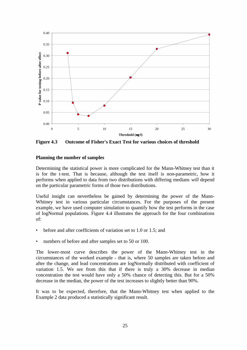
An alternative way of testing whether the improvement is statistically significant is provided by Fisher’s Exact Test. This tests whether the proportions of samples above some specified limit, or ‘threshold’, are significantly different before and after dosing. The threshold may be any desired value, but must be chosen at the outset (rather than be suggested by the data). For example, if the threshold is set at 10 µg/l in the example shown earlier, 28 out of the 50 samples exceed the threshold in the pre-dosing period, but only 20 out of 50 exceed the threshold after dosing. Fisher’s Exact Test then determines how likely it is that the two proportions could be as different as 28/50 and 20/50. The one-sided significance probability in this case is 0.08, which means that the improvement is not significant at the P<0.05 level.

One complication with this test is that the outcome depends on the choice of threshold. This is illustrated in Figure 4.3, which shows the effect of re-applying Fisher’s Exact Test to the example of Figure 4.2 with various thresholds ranging from 30 µg/l down to 3 µg/l. For a narrow window between about 5 and 8 µg/l, the test is significant at the P<0.05 level, but otherwise is not.

In particular, we see that the Fisher’s Exact Test approaches the significance level achieved by the Mann-Whitney test only when the threshold is 7 µg/l, and otherwise provides a weaker assessment of the before-after effect. This was to be expected: a threshold-exceedence test makes less use of the data than does a ranking-based method such as the Mann-Whitney test, and so will generally have a poorer statistical power. For this reason, we have not discussed Fisher’s Exact Test further in this report.

25

0.00

0.05

0.10

0.15

0.20

0.25

0.30

0.35

0.40

0 5 10 15 20 25 30

Threshold (µµg/l)

P v

alue

for

tes

ting

bef

ore-

afte

r ef

fect

Figure 4.3 Outcome of Fisher's Exact Test for various choices of threshold

Planning the number of samples

Determining the statistical power is more complicated for the Mann-Whitney test than it is for the t-test. That is because, although the test itself is non-parametric, how it performs when applied to data from two distributions with differing medians will depend on the particular parametric forms of those two distributions.

Useful insight can nevertheless be gained by determining the power of the Mann-Whitney test in various particular circumstances. For the purposes of the present example, we have used computer simulation to quantify how the test performs in the case of logNormal populations. Figure 4.4 illustrates the approach for the four combinations of:

• before and after coefficients of variation set to 1.0 or 1.5; and

• numbers of before and after samples set to 50 or 100.

The lower-most curve describes the power of the Mann-Whitney test in the circumstances of the worked example - that is, where 50 samples are taken before and after the change, and lead concentrations are logNormally distributed with coefficient of variation 1.5. We see from this that if there is truly a 30% decrease in median concentration the test would have only a 50% chance of detecting this. But for a 50% decrease in the median, the power of the test increases to slightly better than 90%.

It was to be expected, therefore, that the Mann-Whitney test when applied to the Example 2 data produced a statistically significant result.

26

It should be noted that the power calculations shown here are only illustrative. Although the two particular CoV values used here were based on actual RDT data, they will not be generally applicable, and so it is important that companies develop measures of variability specific to their own circumstances through the analysis of relevant RDT data.

0

10

20

30

40

50

60

70

80

90

100

0 5 10 15 20 25 30 35 40 45 50

True before-after decrease in median (%)

Pro

b. o

f ob

tain

ing

a st

at.s

ig. d

ecre

ase

(%)

nB=nA =50; CoV=1.0 nB=nA=50; CoV=1.5

nB=nA=100; CoV=1.0 nB=nA=100; CoV=1.5

Figure 4.4 Illustrative statistical power curves for the Mann-Whitney test

27

5. DISCUSSION

It is clear from the information presented in Section 2 that different companies have adopted different approaches to monitoring in relation to optimisation of plumbosolvency treatment. Companies have adopted 30MS sampling from fixed properties in distribution, RDT sampling or pipe rigs in distribution. Most companies are using pipe rigs either as the principal monitoring method or to supplement the results of sampling from properties. The precise mode of operation of pipe rigs is unclear for some companies. There is fairly wide variation in the number of monitoring points chosen per scheme. There is also variation in the method and frequency of monitoring of orthophosphate concentrations at the treatment works.

Any of the three types of sample, or a combination, can be used to assess the effects of changes in treatment on lead concentrations. The principal issues are to ensure

• an adequate number of sampling points and an adequate sampling frequency for fixed properties and rigs; and

• an adequate number of samples for RDT monitoring.

The numbers of samples required “before” and “after” can be determined statistically.

The arrangements for reviewing and assessing the data vary between companies. There should be formal arrangements for reviewing the data on a regular and reasonably frequent basis. Statistical analysis as well as graphical representation should be used to assess the effects of changes to treatment.

There are several models of automatic lead pipe rig that are based on the same principle but which differ in detailed design. Different models of pipe rig are used by water companies even within the same water supply zone. There are differences in the way that lead pipe rigs are operated by different companies.

The arrangements for monitoring the orthophosphate dosed at the treatment works vary from company to company and between schemes. Proper control of orthophosphate dosing is critical to obtaining effective treatment, and to obtaining lead monitoring results that are not influenced by unplanned changes in orthophosphate concentration. On-line monitoring and control should be considered for all treatment plants on a case by case basis.

29

6. TOPICS FOR FURTHER REVIEW

This project has identified a number of issues that merit further review as listed below.

Lead pipe rigs

• practical aspects of siting, operation and maintenance;

• reproducibility of results from individual rigs and between rigs installed in different parts of a water supply area; and

• comparability of results, and trends in results, between pipe rig and fixed-point and RDT samples within water supply areas.

It is anticipated that these aspects would be addressed by means of a number of site visits and analysis of water company data. Experimental work is not proposed at this stage.

Statistical assessment of water company data

Data for RDT, fixed-point samples and pipe rigs should be obtained from a number of companies and analysed to assist in identifying, for example:

• the number of RDT samples required to give the same statistical power as fixed-point (or rig) samples;

• the effect of the proportion of lead-plumbed properties on the statistical power of RDT samples;

• the time required for lead concentrations to stabilise in relation to water characteristics and methods of operation and monitoring;

• methods for dealing with seasonal effects;

• methods for relating or ‘translating’ mean changes in fixed-point data to changes in RDT compliance values;

• methods for dealing with possible changes in variability as lead concentrations are reduced; and

• the extent to which small changes in lead concentrations can be detected and consequently what change in lead concentrations can be considered practically significant in terms of optimisation.

31

APPENDIX A WATER COMPANY MONITORING ARRANGEMENTS

A.1 Company A

A.1.1 Lead monitoring

Monitoring is carried out at between four and nine fixed properties in distribution. 60MS samples are taken by consumers once a month. In addition to lead, orthophosphate, pH and conductivity are measured. Compliance RDT samples are also taken but the results are not used for the purpose of treatment optimisation.

The company’s Lead Strategy Working Group reviews the results at four to six week intervals.

Statistical analysis is not carried out as the database is small (four to nine properties per zone). Trends in monthly average lead concentrations are monitored.

In the longer term it is proposed to discontinue the fixed property sampling and use compliance RDT sampling to monitor the effectiveness of treatment.

A.1.2 Lead pipe rigs

Pipe rigs are not used.

A.1.3 Orthophosphate monitoring

On-line orthophosphate analysers are installed at treatment works.

A.2 Company B


For one scheme 30MS samples were taken weekly from ten fixed properties; that trial has now ceased. For the other five schemes RDT samples are taken from random properties at a frequency of 84 to 420 per year depending on zone size. Orthophosphate, pH and temperature are also measured.

RDT sample data are reviewed as necessary and results greater than 10 µg/l are flagged for investigation.

Paired t-test or Welsh’s unpaired test analysis, as appropriate, have been applied to 30MS and RDT results.

32

In the longer term it is proposed to use RDT sampling at an enhanced frequency.


A total of eight Bury Pumps rigs are installed in use for two of the schemes; these rigs do not fall within the scope of the company’s RPoW. For each scheme, rigs are installed at the treatment plant pre- and post- orthophosphate dosing, with the other two rigs located within distribution. Pipe rig results are reviewed weekly.

The rigs operate to the manufacturer’s default conditions, viz. flow rate 500 ml/minute, flush, 30 minutes stagnation, sample. The rigs operate from 07:00 to 18:00 hours.


Daily grab samples are analysed for orthophosphate.

A.3 Company C


30MS lead samples are taken from between one and three fixed properties per scheme on a weekly basis. RDT samples are also taken from random properties monthly. Orthophosphate, pH, alkalinity and temperature are also measured. 30MS samples are also taken weekly from lead pipe rigs located at the treatment works and/or within distribution.

The results are reviewed graphically. No statistical analysis is performed.

It is proposed to maintain the current monitoring approach in the longer term.


Three Bury Pumps rigs are used to take 30MS samples according to the manufacturers’ default operational programmes.


On-line monitors are installed at two of the three schemes and grab samples are analysed weekly. For the third scheme, samples are analysed every six weeks.

33

A.4 Company D


Lead monitoring is based on the use of 30MS samples from lead pipe rigs plus RDT samples from random and fixed properties. Seventeen Onsite Water Treatment Services (OWTS) rigs are installed in locations in distribution that represent water quality from a number of water treatment works. Between one and nine pipe rigs (OWTS) are installed in distribution for each scheme. The frequency of RDT sampling varies with zone population from 100 (single works/zone) to 1700 (19 zones) per year.

Orthophosphate, pH, alkalinity and temperature are measured in addition to lead.

Orthophosphate and lead results at sources and in the distribution system are reviewed and reported monthly.

The percentage of samples above set values (e.g. 10 µg/l and 25 µg/l) are monitored as are the 3 month rolling mean of lead concentrations in samples collected from individual water quality zones.

No longer term monitoring arrangements have been proposed.


OWTS rigs, which are made to an in-house design, are used. These are programmed to operate from 07:00 to 23:00 hours and to stagnate overnight. The operating sequence is flush for 90 minutes, stagnate for 30 minutes and sample for 40 seconds.


Grab samples are analysed for orthophosphate weekly. Two (of seven) schemes employ on-line orthophosphate analysers.

A.5 Company E


It is proposed to use three Measurement and Control Services (MCS) lead pipe rigs in distribution for each scheme. These will be programmed to take 60MS lead samples and will be sampled twice weekly. RDT samples will also be taken twice weekly (from an unspecified number of properties).

In the longer term the pipe rigs may be decommissioned and the frequency of RDT sampling will be reduced.

34


It is proposed to use MCS pipe rigs, programmed to take 60MS samples.


No information is available.

A.6 Company F


Monitoring is carried out at fixed properties within distribution. Between two and five sites per scheme are sampled weekly for 30MS lead, orthophosphate, pH, alkalinity and temperature over two ten-week periods in a year. Some employee properties are also sampled. RDT lead compliance samples are also taken at a frequency that depends on zone size; at least 100 samples per year will be taken for each scheme. Orthophosphate is measured in RDT samples.

The project support technician downloads laboratory data on a weekly basis for all the types of monitoring listed above with the exception of the RDT data. This includes telemetry plots of phosphate monitor readings. This weekly check enables detection of any significant events such as variations in dosing or unusual lead values and ensures rapid resolution. The zonal RDT data are downloaded on a monthly basis and processed to give an indication of the current compliance with the incoming interim and final standards.

In addition to the weekly check, lead rig results and dosing performance in the form of a faults log is assessed monthly with reports submitted to the Treatment Managers responsible for the sites. Quarterly review meetings are held between the project manger, the operational science manager and the regulatory scientist. Progress reports are submitted that review the dosing performance and the lead values from the monitoring described above. These reviews determine the requirement for any changes or additional measures.

Computational analysis of the data is conducted and although not recognised as a ‘model’, could be developed.

For each scheme a non-linear (power) regression of 30MS lead versus orthophosphate concentration is carried out. A similar analysis is performed on pipe rig data. (In effect this is a regression curve through two or three clusters of data obtained with different target orthophosphate doses but with possible variability in the orthophosphate concentration within each cluster.) This technique has developed over the period of the project so far and is still under consideration as one of the elements of the combined approach to demonstrating optimisation.

35

Other methods under consideration include the "Mann Whitney Wilcoxon" test. The potential effectiveness has been tested on two zones (one that receives phosphate dosed water and one that does not). This demonstrated that differences in results were not due to random variation but did not quantify the effect. In addition, further methods including simple comparisons of arithmetic mean, mode and median to quantify the benefits and support the findings will be considered.

The company’s long-term monitoring strategy is not finalised but is likely to include pipe rigs, lead and orthophosphate monitoring at properties and orthophosphate monitoring at the treatment works.


One Bury Pumps pipe rig is installed at each water treatment works. These are used to take weekly 30MS samples. The rigs are set-up on a 30 minute flush, 30 minute stagnation cycle from 07:00 to 19:00 hours, with overnight stagnation. The company is in the process of installing a total of 40 pipe rigs at strategic locations within distribution. Orthophosphate, pH, alkalinity and temperature are measured in addition to lead.


On-line orthophosphate analysers are installed at each water treatment works. In addition, grab samples are analysed in the laboratory. The frequency of grab samples varies from daily to weekly, depending on the scheme.

Orthophosphate is measured with each fixed property 30MS lead sample.

A.7 Company G


Pipe rigs in distribution are used to take 30MS lead samples (only) once or twice weekly. Either one or two rigs are used per scheme. RDT lead, orthophosphate, alkalinity and temperature are also taken at a frequency of 25 samples per scheme per year.

In the longer term it is proposed to continue monitoring using 30MS pipe rig samples supported by RDT sampling but the sampling frequency may be reduced.


A total of six Bury Pumps pipe rigs are located in distribution and are used to take 30MS samples.

36


Orthophosphate concentrations are measured in weekly grab samples.

A.8 Company H


Monitoring is based on up to four pipe rigs per scheme, located in distribution and up to five rigs at the treatment works. 30MS samples are taken together with samples for orthophosphate, pH, alkalinity and temperature. The rigs are sampled one to four times per month.

In the longer term the sampling frequency will be reduced to monthly.


A comparative trial of Bury and Prominent rigs was carried out, on the basis of which it was decided to use Bury rigs. These are set to take 30MS samples with a 6 minute gap between stagnations during the day, and an 8-hour overnight stagnation.


Orthophosphate concentrations are measured daily at each treatment works using test kits.

A.9 Company I


MCS pipe rigs installed in roadside kiosks are used for lead monitoring in distribution. Between one and four rigs are in use for each scheme; four 60MS samples are taken in clusters on successive days each month. RDT samples taken from random properties are used to supplement the rig data. These samples are analysed for lead, pH and orthophosphate. The frequency of random sampling varies from 52 to 132 per year, depending on zone size.

The data from the lead rigs is plotted onto line graphs (lead and orthophosphate versus date), showing orthophosphate dose targets, actual dose rates at treatment works and lead concentrations from the rigs in distribution. The graphs are updated weekly by water quality, and issued monthly to production and network departments to ensure that all sections involved are fully aware of the project. Results of customer property samples are updated and circulated quarterly.

37

Statistical analysis of the data has not been carried out.

In the longer term it is anticipated that the pipe rigs will be removed and that random samples will be used for monitoring.


MCS pipe rigs are used in distribution. These are programmed to take 60MS samples. The rigs operate for 12 hours per day, with overnight stagnation.


Test kits are used to measure orthophosphate concentrations and laboratory analyses are performed weekly.

GIS software is used to plot orthophosphate concentrations across a supply zone.

A.10 Company J


The monitoring is based on RDT samples from random properties, 30MS stagnation from fixed properties and 30MS samples from pipe rigs. There are up to 30 fixed properties per scheme. At least one sample is taken per week for each scheme. In the case of pipe rig samples, temperature, orthophosphate, pH, turbidity and 30MS lead are measured weekly; TOC and alkalinity are measured monthly.

The results for lead (stagnation and second draw) and orthophosphate are represented graphically on the company’s Intranet. Any second draw lead sample >10 µg/l or orthophosphate concentration <1.7 mg/l P or >2.2 mg/l P will generate an exception report. Statistical assessment of the results is not carried out.

Lead pipe rigs and RDT sampling will continue to be used for the foreseeable future.


Hydraulics Modelling Services (HMS) and Prominent rigs are used in the distribution system. With the HMS rigs, in between each 30 minute stagnation period there is a 3 second purge to waste, 50 second purge to the sample bottle and a 50 second flush to waste. With the Prominent rigs, in between each 30 minute stagnation period there is a 30 second purge to the sample bottle and a 45 second flush to waste. No changes have been made to the manufacturers’ settings.

38


Grab samples are taken at least weekly for analysis.

A.11 Company K


Monitoring is carried out at between two and four fixed properties per scheme. Monthly samples are taken for 30MS lead, pH, alkalinity, orthophosphate, colour and temperature. Pipe rigs located in distribution are also used to take 30MS samples.

The results are extracted automatically on a quarterly basis and graphed.

The company does not have a strategy for monitoring in the longer term.


One or two pipe rigs (in-house “Sentry” or Sheers) are located in distribution for each scheme. 30MS samples are taken monthly. The Sentry rigs are operated manually with flushing followed by 30 minutes stagnation.


On-line orthophosphate analysers are installed at water treatment works. Grab samples are analysed in the operations laboratory either daily (surface waters) or weekly (groundwaters) and in the main analytical laboratory weekly.

A.12 Company L


RDT samples are taken at a frequency of 520 per annum in the distribution zone. These are analysed for lead, orthophosphate and temperature (iron and manganese are also measured on these samples for reasons unconnected with plumbosolvency control). Properties identified as having lead pipes are sampled.

The results of RDT sampling for the six months before and after commencing orthophosphate dosing have been compared. In the future the data will be reviewed on a quarterly basis. Summary statistics (mean, maximum, minimum and median) are calculated, together with the number of samples that exceed 10 and 25 µg/l.

39


No pipe rigs are in use.


An on-line orthophosphate analyser is installed at the water treatment works.

A.13 Company M


RDT lead samples are taken from random properties. The sampling frequency is from 12 to 48 per zone per year – this equates to 12 to 684 samples per scheme per year. Orthophosphate, pH, conductivity, iron and temperature are also measured.

All RDT results are plotted on a sequential graphical plot. From visual inspection the performance of each scheme is evaluated through time and the performance of other schemes are evaluated against each other. An increase in the number of RDT samples exceeding established thresholds (e.g. 10 µg/l) will indicate individual scheme poor performance. In addition to the visual monitoring, the significance of pass/fail ratios, either through time for an individual schemes basis or on an inter-scheme basis, will be evaluated using the Fisher Exact test.


Pipe rigs (one Aqualine, one Prominent) are installed at two of the company’s treatment works. These are set up to take 30MS samples, which are collected three times per week. The operational cycles are:

Aqualine Prominent

On 06:00, off 10:30 On 14:00, off 16:00 On 18:00, off 20:00 On 03:00, off 04:30 30 min flush, 30 min stagnation, 24 sec sampling.

On 06:00, off 10:00 On 12:00, off 15:00 On 18:00, off 22:00 30 min flush, 30 min stagnation, 22 sec sampling.


Grab samples are analysed for orthophosphate daily, five times per week or every other day.

40

A.14 Company N


RDT samples are taken from random properties in distribution. Fifty samples per zone per year are taken. Orthophosphate and pH are measured in addition to lead. Two lead pipe rigs are located in distribution for each scheme. These take 30MS samples which are collected weekly. Orthophosphate, pH, alkalinity, colour and temperature are also measured on the rig samples.

RDT results are reviewed monthly. Lead pipe rig results are reviewed weekly.

The Mann-Whitney U test is used to analyse the RDT data.

Computer modelling is used as part of the optimisation strategy but this does not have a direct bearing on the monitoring strategy.

In the longer term both RDT sampling and pipe rigs will be used to confirm and maintain optimum conditions.


Two Bury Pumps rigs are installed in distribution for each scheme. In accordance with the manufacturer's default operating condition, the flow rate is 500 ml/min, the sample time is 23 seconds and the stagnation time is 30 minutes. The flushing time, which was not specified by the manufacturer, has been set by the company at 4 minutes.


Grab samples are taken at least weekly and analysed using test kits.

A.15 Company O


The Company uses lead pipe rigs in distribution to monitor lead concentrations. 30MS lead concentrations plus pH, orthophosphate, alkalinity and temperature are measured weekly. Either two or three rigs are used per scheme. Compliance sampling for RDT lead, orthophosphate, pH, alkalinity and temperature is undertaken for comparative purposes.

Results from all rigs within a distribution area are compared graphically to assess comparability of each parameter between the rigs. These assessments are made on a monthly basis. The results are plotted against time as instantaneous values and as four-week moving averages. Assessment of trends is then made on a visual basis.

41

In the longer term, it is proposed to take at least two RDT samples per month for each zone. Consideration will be given to maintaining the lead pipe rigs.


A total of eight OWTS (previously Meridian Science) pipe rigs are deployed in distribution. These are used to take 30MS samples, with a 2 hour interval with continuous discharge (flush) between each stagnation, with 24 hour operation.


On-line analysers are installed at all orthophosphate dosing plants. Daily grab samples are also measured using test kits.

A.16 Company P


Lead monitoring is achieved using lead pipe rigs in distribution. Between one and seven rigs per scheme are sampled weekly for 8 hour stagnation lead, orthophosphate and temperature. For each scheme a pipe rig is also installed at the treatment works. The stability of lead concentrations at customer properties will be assessed after optimisation has been achieved by taking at least 96 RDT samples per year for each scheme.

A dedicated technician is responsible for monitoring and review of data from the lead pipe rigs installed at treatment works and in supply zones.

At present visual assessment is made of time series plots of lead concentrations. Statistical tests may be applied in the future.

The longer term monitoring strategy has not been determined.


Bury Pumps, Enercell and PDL pipe rigs are used. These are set to flush for 16 hours followed by 8 hours stagnation. The rigs are located both at the treatment plant and within distribution.


On-line orthophosphate analysers are installed at each treatment works. Grab samples are also measured using test kits.

42

A.17 Company Q


Between one and nine fixed properties are sampled in clusters of three samples once per month. RDT, FF and 30MS lead samples are taken. Orthophosphate, pH, alkalinity and temperature are also measured. Up to four pipe rigs are installed in distribution, and rigs are installed at some water treatment works. Three samples are taken from the rigs in clusters, either weekly or fortnightly.

Lead stagnation sample data are reviewed every two months. It is planned to review the RDT data on a quarterly basis. Treatment works orthophosphate concentrations are reviewed weekly. Statistical techniques have not yet been applied to the data.

A strategy for monitoring in the longer term has not been developed.


Prominent and Bury Pumps pipe rigs are used. The rigs operate continuously, collecting 30MS samples.


Grab samples are analysed for orthophosphate at a frequency of three or five per week. On-line orthophosphate monitoring is being considered.

A.18 Company R


Monitoring is carried out at fixed properties within distribution. Between two and ten sites per scheme are sampled three times per month for 30MS lead (total, and dissolved), orthophosphate and temperature. In addition, a lead (RDT) sample is taken each time a compliance bacteriological sample is taken; pH, orthophosphate, alkalinity, iron and temperature are also measured. One lead pipe rig is installed in distribution.

The WRc-NSF “WaQCoM” computer model is used to predict the benefits of optimisation (this model is not directly relevant to the monitoring strategy).

Summary statistics (minimum, maximum, mean and percentiles) are prepared for lead and orthophosphate concentrations.

In the longer term sampling will continue at all treated water lead test rigs and monitoring will continue at a reduced number of fixed-point domestic properties.

43


Two types of rigs are in use, supplied by Prominent (two rigs) and HMS (3 rigs). One HMS rig is installed in distribution, the remainder are sited at water treatment works (at one works, one rig before and after orthophosphate dosing). Each rig consists of a 3 metre length of ½ inch lead pipework with associated control valves and sample chamber. One Prominent rig is set to take 8 hour stagnation samples; all of the other rigs take 30MS samples. The rigs operate continuously at the manufacturers’ default settings.

At the selected interval, the rig runs its sampling programme as follows:

i) Flushing valve opens, to flush from the rig any water retained in the lead pipe; this water is discharged to waste. The flow through the rig is controlled through a Maric flow-control valve (Prominent rig) or needle valve (HMS rig).

ii) Flushing valve closes and water is retained in the lead pipe for a chosen stagnation period.

iii) After this period, a sample valve opens to discharge the retained water into a sample collection chamber. The volume of the chamber is 1 litre, which requires three sample sequences before the chamber begins to overflow to waste. The chamber fills from the bottom and the overflow is from the top, so incoming freshly stagnated water displaces previously-sampled water when the sample chamber begins to overflow.


On-line orthophosphate analysers are installed at each treatment works. Grab samples, taken either daily or five times per week, are analysed in the laboratory.

Samples for orthophosphate analysis are taken with all lead samples.

A.19 Company S


Monitoring is carried out at random properties using RDT sampling. The sampling frequency is eight samples per zone per month. Orthophosphate, pH, alkalinity, TOC and iron are also monitored extensively.

The data will be entered into a lead database on a weekly basis. This can be linked to the company’s GIS system to examine the data geographically as well as in spreadsheet format.

Statistical treatment of the data is at an early stage but it is planned to use a combination of Shewhart control charts, Cusum charts, Manhattan diagrams and compliance records

44

to assess the data. It is also planned to use non-parametric statistics to analyse the lead data.


A total of 25 pipe rigs are located within distribution and 13 at water treatment works. The OWTS rigs are programmed to flush for 89 minutes, stagnate for 30 minutes then sample (40 seconds). The rigs have only recently been commissioned (February 2003). It is planned to take samples weekly for lead and orthophosphate. The pipe rig data will be used as a secondary source of information to the RDT sampling to demonstrate optimisation.


Grab samples are analysed weekly. On-line orthophosphate monitors are installed at a few works.

A.20 Company T


Monitoring is carried out at fixed properties in distribution. Between four and 12 sites per scheme are sampled monthly for RDT, fully flushed (FF) and 30MS lead and pH, orthophosphate, and temperature. Compliance RDT samples are also taken. Lead pipe rigs installed in distribution are sampled weekly for 30MS lead.

All of the lead results are collated every three months and used to update the performance assessments.

The mean pre-orthophosphate and post-orthophosphate 30MS results for each fixed property are tabulated together with the percentage reduction in lead concentrations; the zone means are also tabulated. The data for pipe rigs are treated in a similar manner. For each scheme, the percent of RDT samples greater than 25 µg/l and 10 µg/l are tabulated for each change in orthophosphate dose.

Computational zonal modelling has been used to estimate the reduction in lead concentrations required to achieve compliance; this does not have a direct bearing on monitoring strategy.

The Company plans to cease monitoring at fixed properties in distribution once optimisation has been achieved. The pipe rigs will be retained but with a reduced sampling frequency (monthly).

45


There is a total of 32 pipe rigs of which three are manufactured by Prominent (all used for the same scheme) and 29 by Bury pumps. Up to eight rigs are installed at treatment works (pre- and post-orthophosphate dosing). One scheme has 10 rigs in distribution; the remainder have one rig per scheme. 30MS samples are taken weekly, orthophosphate and pH are also measured..

The rigs operate continuously with a cycle of 30 minutes flush, 30 minutes stagnation and 23 seconds sampling. The flushing time has been adjusted from the manufacturers’ default settings – this was done following an investigation that demonstrated that the default flush time was too short resulting in elevated lead concentrations.


Grab samples are taken twice weekly for laboratory analysis.

A.21 Company U


Pipe rigs in distribution are sampled for 30MS lead, pH, orthophosphate and temperature on a weekly basis. There are between one and three rigs per scheme. RDT compliance samples are taken at the regulatory frequency.

The lead, orthophosphate and pH data are reviewed on a monthly basis. Time series plots are used to examine the results.

In the longer term the use of pipe rigs may be discontinued once optimisation has been achieved.


Prominent and HMS rigs are used. These operate continuously using the manufacturers’ default conditions and take 30MS samples, with the time between stagnation set at 30 minutes. The rigs are sampled weekly. Orthophosphate and pH are measured in addition to lead.


All plants have on-line orthophosphate analysers. Grab samples are taken weekly for laboratory analysis.

46

A22 Company V


Lead samples are taken monthly from up to five fixed properties in distribution. An RDT sample is taken on arrival followed by a FF and a 30MS sample. Up to three Prominent lead pipe rigs are located in distribution, plus one at each water treatment works. 30MS rig samples are collected weekly. For both fixed properties and rigs, the FF sample is analysed for lead, orthophosphate, pH and temperature. Compliance RDT samples are taken for lead and orthophosphate at a frequency that depends on zone size.

Results from monitoring are reviewed by an internal Lead Group consisting of scientists from each of the three operational areas. All monitoring points – works and distribution lead rigs and leaded customer properties – have been set up as time series graphs showing stagnation lead, orthophosphate and temperature and these are continuously updated and available to view on a shared computer drive.

Statistical analysis is not used.

Computational zonal modelling has been used; this does not have a direct bearing on monitoring strategy.

In the longer term it is anticipated that sampling from fixed properties will cease.


Prominent pipe rigs are used both at treatment works and in distribution. These operate on a continuous cycle of 4 minutes flush, 30 minute stagnate, 23 second sample, 90 minute stagnation. A few rigs in distribution do not operate at night or at weekends.


Samples are analysed for orthophosphate using test kits daily and weekly samples are taken for laboratory analysis. An on-line monitor is installed at one treatment works.

A.23 Company W


Monitoring is carried out at between one and 14 fixed properties per scheme. Overnight (“8 hour”) stagnation samples are taken by householders. The samples are taken in clusters of three in a week, every three months. Lead pipe rigs (in-house built) are used to taker 30MS samples weekly. Typically one rig is located at the treatment works and from one to six in distribution. Total and soluble lead, orthophosphate, pH, alkalinity and

47

DOC are measured. For small supply zones (population <730) RDT sampling at an enhanced frequency is used.

Monitoring data from the works, pipe rigs, customer stagnation samples and RDTs are formally reviewed on a monthly basis.

Statistical assessment of RDT results has been used to assess the likelihood of failing to achieve 10 µg/l.

In the longer term monitoring will continue as at present although drop-out of fixed properties is anticipated.


In-house built manually operated lead pipe rigs are used within distribution and at treatment works. These are used to take weekly 30MS samples.


On-line orthophosphate analysers are in use. Grab samples are taken at a frequency from daily to weekly for laboratory analysis.

49

APPENDIX B PIPE RIG TECHNICAL DATA

B.1 AUTOMATIC LEAD PIPE RIGS

B.1.1 General

A number of automatically operated lead pipe rigs are commercially available. Whilst these differ in detailed design, they are all based on the principles outlined in Information Letter 02/90. The rig consists of a single lead pipe arranged to produce stagnation samples automatically, ready for collection by a sampler at any time. A schematic diagram of an automatic lead pipe rig is given in Figure B.1. All the components are mounted on a board or in a cabinet (“kiosk”).

The rig is connected to the water supply to be monitored. The water flows through a non-return valve and strainer to a constant flow rate valve and flow meter. The flow rate is set at a fixed rate when either of the outlet solenoid valves is open. The water then flows through a 3 metre length of lead pipe. For compactness the lead pipe is coiled in a gentle S-shape. Finally the water can either flow to waste directly through a solenoid valve or alternatively through another solenoid valve to waste via the sample vessel.

The storage capacity of the sample vessel to its overflow does not have to be limited by the volume of the lead pipe. This volume limits the time the solenoid valve to the sample vessel is open. For example, 3 m of ½ inch diameter lead pipe has a volume of approximately 400 ml; thus for a flow rate setting of 500 ml/minute, the solenoid valve should not be open for more than 45 seconds before the next flush and stagnation sample is started. It then follows that a sample vessel of one litre can be used even though it will take at least three flush and stagnation cycles to fill or displace it. The vessel has a conical base into which the inlet protrudes. Thus, incoming freshly stagnated water displaces previously sampled water. The sampler draws a sample from the tap connected to the base of the sample vessel.

Details of particular models are provided below.

50

1 Water inlet 2 Flow control valve 3 Flow meter 4 Pipe connectors 5 Lead pipe 6 Solenoid valves 7 Sample container 8 Sample valve 9 Flush (to waste) 10 Control panel / timer

Figure B.1 General arrangement of automatic pipe rigs

B.1.2 Aqualine Engineering Services

The Automatic Lead Sampler consists of a lead coil through which water flows via a non-return valve and flow meter. The system operates in three time zones:

1. Flushing 2. Stagnation 3. Sampling

The stagnated water is collected in a plastic receiver. The conical base of the receiver allows new samples to displace the previously collected water. A sample for analysis can be tapped off externally via a valve at the base of the unit.

B.1.3 Bury Pumps

Bury Pumps Limited in conjunction with Anglian Water have developed a lead test rig to automatically sample the water supply by taking samples of stagnated water at regular intervals over a 24 hour period. The unit consists of a three metre length of ½ inch nominal bore lead pipe through which water flows via a non-return valve and flow meter. The system operates in three time zones;

1. Flushing 2. Stagnation

9 8

7 6

6

5

4

4

3

2

1

10

51

3. Sampling

A Programmable Logic Controller (PLC) controls all the time zones with built in 24-hour timer. The PLC opens solenoid valves accordingly. During sampling some of the stagnated water is collected in a conical plastic receiver. The conical base of the receiver allows new samples to displace the previously collected water out through the overflow. A sample for analysis can be tapped off externally via a stopcock at the base of the unit.

To combat condensation within the unit a fan has been fitted to pass fresh air through the unit. For safety an isolation switch has been fitted within the unit. Wall brackets allow the unit to be surfaced mounted. For areas of low water pressure a header tank and pump can be used to provide adequate flows. The pump is controlled by the PLC so that it only operates during the appropriate time zone.

The timer can be programmed for various timed operations within a 24-hour period. Typically only one operation will be used e.g. on 7.00 am, off 6.00 pm. This will simulate an 11 hours on, 13 hours off cycle to simulate household usage. When the system is in operation the PLC introduces a three-operation cycle and takes over control of the rig.

The flow meter fitted in all units is capable of controlling flow in the range 50 to 800 ml/min. A recommended flow rate is 500 ml/min. This is achieved using standard water pressure inlet and turning the flow adjustment to increase or decrease the flow. The top of the float in the sight glass indicates the flow through the rig. To ensure that the sample taken only contains stagnated water the sample time must be set to the correct setting.

B.1.4 Enercell

The rig (product number EN1006LTR) is designed to hold water in a 3 metre length of ½ inch lead pipe for a set stagnation period, normally set at between 8 and 12 hours. A sample is then taken into the sample pot. When not stagnating or sampling the rig is flushed continuously. The sampling stage takes 46 seconds at the recommended flowrate of 250 ml/min. The sample is manually decanted using the sample valve at the bottom of the rig.

B.1.5 Hydraulics Modelling Services (HMS)

The unit comes pre-programmed to run a 30-minute stagnation cycle. The cycle times can be modified. The supply water or sample enters the unit through the ½ inch PVC socket on the bottom left side of the unit. The sample, once in the unit, passes through an isolating ball valve followed by a pressure reducing valve, check valve and flow meter with needle valve. The needle valve is used to adjust the flow, normally to 400 ml/min.

The sample then passes through 3 metres of new lead pipe (O.D. 23.5 mm, I.D. 12.5 mm). Two solenoid valves control the direction of flow downstream of the lead pipe. The flushing valve sends sample to waste. The sampling valve sends flow into a sampling container. Here the sample is stored and is constantly replenished as the unit

52

goes through its continuous 30-minute stagnation cycles. Fresh sample enters the vessel at the bottom to displace existing sample via the overflow.

The basic stagnation cycle supplied with the unit is as follows:

1. Flushing valve opens for 50 seconds 2. Flushing valve closes 3. After 30 minutes the flushing valve opens for 3 seconds to clear the pipe work

between the end of the lead pipe and the inlet of the sampling solenoid valve 4. Flushing valve closes 5. Sampling valve opens for 50 seconds to allow only sample which has been in

contact with the lead for 30 minutes to enter the sampling container 6. Sample valve closes 7. Return to 1

B.1.6 Measurement and Control Services (MCS)

The FA67 lead test rig is designed to be located within the distribution system. The rig is housed in a green GRP kiosk and is powered by a 24 V DC battery pack designed to last for one week.

The rig is connected to the water supply, water flows through an isolation valve, non-return valve, strainer, flow regulating valve, flow meter to a 3 metre length of ½ inch diameter lead pipe. The flow is controlled by two solenoid valves on the outlet, which allow flow either to waste to flush, or a sample vessel. The water flowrate is 1000 ml/min for approximately 1 minute every 30 or 60 minutes, depending on the stagnation time setting. The sample vessel holds approximately three samples and then overflows to waste. The rig sequence is as follows:

1. Sampling initiated at 6:00 am 2. Flush to waste 3. Stagnate water in lead pipe for 30 or 60 minutes 4. Transfer stagnated water to sample vessel 5. Flush to waste 6. Repeat steps 3 to 5 until 6:00 pm

The operating conditions are as follows:

– Flowrate 1000 ml/min fixed by flow control valve (flowrate indication by flow meter) – Flush time 30 seconds factory set – Sample time 22 seconds factory set – Stagnate time 30 or 60 minutes switch selectable – Operating period 6:00 am to 6:00 pm factory set utilising internal clock

The sample time of 22 seconds is calculated to transfer the volume of water held in 3 m × ½ inch diameter lead p ipe at 1000 ml/min.

53

B.1.7 Onsite Water Treatment Services (OWTS)

The rig uses a 3 metre length of ½ inch lead pipe. A metering valve controls the flow to and through the lead pipe. The stagnated lead sample is stored in a catch pot that is continually refreshed with the latest sample. The stagnation and sample periods are infinitely variable via a Programmable Logic Controller. The operating sequence is as follows:

Flush – During the flush cycle water enters the unit via a double seated check valve, through the metering valve that is used to manually set the flow rate at 500 ml/min. The actual flow rate is shown immediately above the valve on the variable area flow meter. The water then passes through the lead pipe and to drain via a waste solenoid valve.

Stagnation – During this cycle both sample and waste solenoid valves remain closed thus causing the flow through the system to stop. The duration of the stagnation time is infinitely variable and is set within the PLC controller.

Sample –During this cycle the sample solenoid is opened for 40 seconds, which allows all water within the lead pipe to be displaced into the sample catch pot. The sample catch pot inlet pipe is extended to the bottom of the vessel to ensure that the oldest sample is displaced via the overflow. Samples for analysis are collected from the sample tap located at the bottom of the catch pot.

B.1.8 PDL

A 3 metre length of ½ inch lead pipe is used. The unit can be programmed to sample up to 15 times per day. Stagnated water is collected in a sample pot mounted on the front of the rig.

B.1.9 Prominent

The Mk IIA rig (Part No. 7260356) comprises a 3 metre length of ½ inch bore lead pipe mounted on a backboard with ancillary flow control equipment and a self-contained control box. Two solenoid valves govern the flow of water through the unit. The sample valve is opened when a sample is required, the time at which it is taken is pre-programmed into the Programmable Logic Controller (PLC). The PLC also determines the duration of opening of the sample valve. The purge valve is opened when purging is required, the time at which it occurs is pre-programmed into the PLC. The PLC also determines the duration of opening of the purge valve. The factory settings within the PLC are such that the sample valve will open for 24 seconds and the purge valve for 45 seconds. These settings can be altered by re-programming to allow for differing flow rates on specific sites.

The flow rate at which water passes through the System is regulated by a 'Maric'-type constant flow valve, and should be approx. l000 ml/min when the water supply pressure is between 1.5 and 5 bar.

54

The duration of the sample valve opening should equate to a sample volume of 400 ml each time it opens. The sample vessel that it connects to has a volume of 1litre, therefore it will take three sampling periods to initially fill it. Once full, any subsequent sampling will displace the existing sample volume to overflow and then to waste. Stagnation samples are collected via the ball valve at the bottom of the sample chamber when necessary.

An overnight stagnation test is allowed for by the timer control. The rig has two modes: overnight and daytime. Daytime mode is defined by the on and off times set in the clock. The rig can also be used on defined days of the week using this function e.g. if there was no requirement for testing on a Sunday the Time Clock parameters within the PLC could be adjusted to prevent the rig from running on Sunday. The factory settings are for operation 06:00 to 00:30 hours, seven days a week.

B.1.10 Sheers

No detailed information is available.

B.2 Manually operated rigs

Companies K and W employ manually operated pipe rigs. A diagram of the rig is given in Figure B.2. A 2-metre length of lead piping is used.

The operating procedure is as follows:

1. Close outlet valve No1 – Stops water running to drain 2. Open vent valve No4 – Flush the lead pipe system for 1 litre 3. Close vent valve No4 – Stops flushing lead 4. Open vent valve No3 – Flush the lead pipe system for 3 litres 5. Close vent valve No3 – Stops flushing lead pipe 6. Close Inlet valve No2 7. Wait 30 minutes sample time 8. Open vent valve No3 – Allows sample pipe to vent 9. Place sample container under the sample valve No 4 10. Open sample valve No4 11. When water stops running close sample valve No4 12. Close vent valve No3 13. Open outlet valve No1 then open inlet valve No2

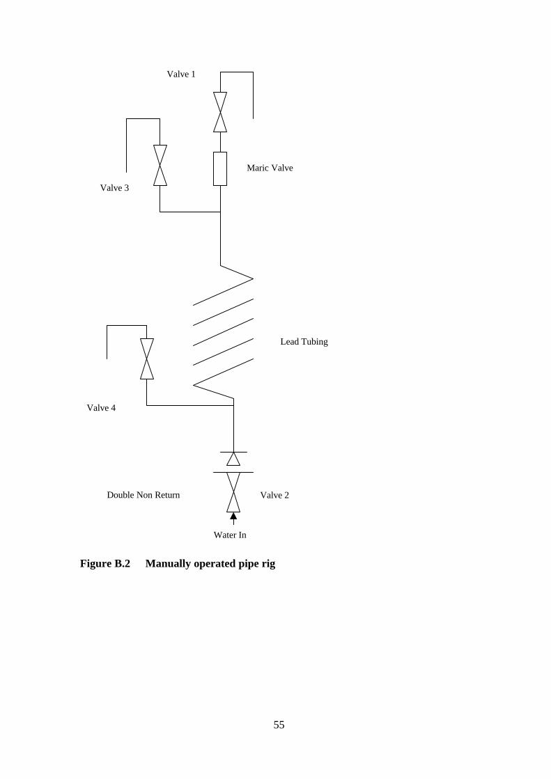
55

Valve 1

Water In

Double Non Return

Lead Tubing

Valve 4

Valve 3

Maric Valve

Valve 2

Figure B.2 Manually operated pipe rig

56

B.3 Contact details

Aqualine Engineering Services

(no details available)

Bury Pumps Ltd Unit 5 Woodlands Business Park Rougham Industrial Estate Bury St. Edmunds Suffolk IP30 9ND

Tel: (01359) 270802 Fax: (01359) 271011 E-mail: [email protected] Web: www.bury-pumps.co.uk

Enercell UK Ltd Prospect House 1 The Hyde Business Park Bevendean Brighton BN2 4JE

Tel: (01273) 888000

Hydraulic Modelling Services Ltd 35 Colville Road Acton W3 8BL

Tel: (020) 8993 6621 Fax: (020) 8993 6621 E-mail: [email protected] Web: www.hmsltduk.com

Measurement and Control Services Ltd. Unit 5 Ashbys Yard Medway Wharf Road Tonbridge TN9 1RE

Tel: (01732) 770885 Fax: (01732) 770886

Onsite Water Treatment Services Wood End Lane Fradley Lichfield WS13 8NF

Tel: (01543) 445700 Fax: (01543) 445717

PDL Arena Engineering Ltd. Unit 6 Swanwick Business Centre Bridge Road Swanwick Southampton SO31 7GB

Tel: (01489) 570470 Fax: (01489) 583332

ProMinent Fluid Controls UK Ltd. Resolution Road Ashby de la Zouch Leicestershire LE65 1DU

Tel: (01530) 560555 Fax: (01530) 560777 E-mail:[email protected] Web: www.prominent.co.uk

demonstration of optimisation of plumbosolvency treatment...

Documents