demonstration of the recent additions in modeling

NREL is a national laboratory of the U.S. Department of Energy Office of Energy Efficiency & Renewable Energy Operated by the Alliance for Sustainable Energy, LLC This report is available at no cost from the National Renewable Energy Laboratory (NREL) at www.nrel.gov/publications.

Contract No. DE-AC36-08GO28308

Demonstration of the Recent Additions in Modeling Capabilities for the WEC-Sim Wave Energy Converter Design Tool Preprint N. Tom, M. Lawson, and Y-H. Yu National Renewable Energy Laboratory

To be presented at the 34th International Conference on Ocean, Offshore, and Arctic Engineering (OMAE 2015) St. John’s, Newfoundland, Canada May 31‒June 5, 2015

Conference Paper NREL/CP-5000-63528 March 2015

NOTICE

The submitted manuscript has been offered by an employee of the Alliance for Sustainable Energy, LLC (Alliance), a contractor of the US Government under Contract No. DE-AC36-08GO28308. Accordingly, the US Government and Alliance retain a nonexclusive royalty-free license to publish or reproduce the published form of this contribution, or allow others to do so, for US Government purposes.

This report was prepared as an account of work sponsored by an agency of the United States government. Neither the United States government nor any agency thereof, nor any of their employees, makes any warranty, express or implied, or assumes any legal liability or responsibility for the accuracy, completeness, or usefulness of any information, apparatus, product, or process disclosed, or represents that its use would not infringe privately owned rights. Reference herein to any specific commercial product, process, or service by trade name, trademark, manufacturer, or otherwise does not necessarily constitute or imply its endorsement, recommendation, or favoring by the United States government or any agency thereof. The views and opinions of authors expressed herein do not necessarily state or reflect those of the United States government or any agency thereof.

This report is available at no cost from the National Renewable Energy Laboratory (NREL) at www.nrel.gov/publications.

Available electronically at http://www.osti.gov/scitech

Available for a processing fee to U.S. Department of Energy and its contractors, in paper, from:

U.S. Department of Energy Office of Scientific and Technical Information P.O. Box 62 Oak Ridge, TN 37831-0062 phone: 865.576.8401 fax: 865.576.5728 email: mailto:[email protected]

Available for sale to the public, in paper, from:

U.S. Department of Commerce National Technical Information Service 5285 Port Royal Road Springfield, VA 22161 phone: 800.553.6847 fax: 703.605.6900 email: [email protected] online ordering: http://www.ntis.gov/help/ordermethods.aspx

Cover Photos: (left to right) photo by Pat Corkery, NREL 16416, photo from SunEdison, NREL 17423, photo by Pat Corkery, NREL 16560, photo by Dennis Schroeder, NREL 17613, photo by Dean Armstrong, NREL 17436, photo by Pat Corkery, NREL 17721.

NREL prints on paper that contains recycled content.

http://www.osti.gov/scitech

mailto:[email protected]

mailto:[email protected]

http://www.ntis.gov/help/ordermethods.aspx

1


DEMONSTRATION OF THE RECENT ADDITIONS IN MODELING CAPABILITIES FOR THE WEC-SIM WAVE ENERGY CONVERTER DESIGN TOOL

Nathan Tom*

National Renewable Energy Laboratory

Golden, Colorado, USA [email protected]

Michael Lawson National Renewable Energy Laboratory


Yi-Hsiang Yu National Renewable Energy Laboratory


*Correspondence author

ABSTRACT WEC-Sim is a midfidelity numerical tool for modeling

wave energy conversion devices. The code uses the MATLAB SimMechanics package to solve multibody dynamics and models wave interactions using hydrodynamic coefficients derived from frequency domain boundary element methods. This paper presents the new modeling features introduced in the latest release of WEC-Sim. The first feature discussed is the conversion of the fluid memory kernel to a state-space approximation that provides significant gains in computational speed. The benefit of the state-space calculation becomes even greater after the hydrodynamic body-to-body coefficients are introduced as the number of interactions increases exponentially with the number of floating bodies. The final feature discussed is the capability to add Morison elements to provide additional hydrodynamic damping and inertia. This is generally used as a tuning feature, because performance is highly dependent on the chosen coefficients. In this paper, a review of the hydrodynamic theory for each of the features is provided and successful implementation is verified using test cases.

INTRODUCTION

During the past decade there has been renewed interest from both the commercial and governmental sectors in the development of marine and hydrokinetic energy. However, wave energy converters (WECs) remain in the early stages of development and have not yet proven to be commercially viable. Given the relatively few full-scale device deployments, WEC development is highly dependent on numerical modeling tools to drive innovative designs and advanced control strategies. Conventional seakeeping software has a difficult

time modeling new multibody WECs. These complications arise because of the various links between bodies and the additional degrees of freedom required to model the power extraction process.

WEC modeling tools are currently being developed by several companies. These include WaveDyn distributed by Det Norske Veritas – Germanischer Lloyd (DNV-GL) [1], OrcaFlex distributed by Orcina [2], AQWA distributed by ANSYS, and INWAVE distributed by INNOSEA [3]. However, it is desirable to develop open-source modeling tools to establish a collaborative research community that can accelerate the pace of technology development. To assist the fledgling U.S. marine and hydrokinetic industry, the U.S. Department of Energy (DOE) [4] funded a joint initiative between the National Renewable Energy Laboratory (NREL) and Sandia National Laboratories (SNL) to develop a comprehensive wave energy modeling tool to assist both the research and industry communities. The joint effort between NREL and SNL led to the release of WEC-Sim-v1.0 [5] in the summer of 2014. The code was developed in the MATLAB/SIMULINK [6] environment using the multibody dynamics solver SimMechanics with preliminary code verification performed in [7] [8]. At the moment, WEC-Sim is best suited to handle rigid multibody dynamics allowing for multiple linkages; however, overtopping and oscillating water column WEC concepts cannot be easily modeled.

This paper provides an overview of the additional modeling capabilities included in WEC-Sim-v1.1 released in March 2015. The first module described is the realization of the fluid memory kernel in state-space form. This ability will help reduce computational time after hydrodynamic body-to-body interactions are introduced. The final hydrodynamic

2


feature described is the inclusion of Morison elements to provide additional inertia and viscous drag forces. The hydrodynamic theory for each feature is provided before results from test cases are used to verify succesful implementation within WEC-Sim.

STATE-SPACE REPRESENTATION OF THE IMPULSE RESPONSE FUNCTION

In linear water wave theory, the instantaneous wave radiation force, commonly known as the Cummins equation [9], can be written as follows:

( )∫∞−

∞∞ −−−−=t

rr dtKtttf ttζtζλζµ )()()()( (1)

where μ∞ is the added mass at infinite frequency, λ∞ is the wave damping at infinite frequency, Kr is a causal function known as the radiation impulse-response function, and ζ is the six-degrees-of-freedom vector of body motion. The convolution term in Eqn. (1) captures the effect that the changes in momentum of the fluid at a particular time affect the motion at future instances, which can be thought of as a fluid memory effect. The relationship between the time- and frequency- domain coefficients were derived in [10], as follows:

( )∫∞

∞ +=0

cos)( tdttK r sλsλ (2)

∫∞

∞ −=0

sin)(1)( tdttK r ss

µsµ (3)

where μ(σ) and λ(σ) are the frequency dependent hydrodynamic radiation coefficients commonly known as the added mass and wave damping.

The radiation impulse response function can be calculated by taking the inverse Fourier transform of the hydrodynamic radiation coefficients, as found by

[ ] ssµsµsπ

tdtK r sin)(2)(0∫∞

∞−−= (4)

[ ]∫ −=∞

∞0

cos)(2)( ssλsλπ tdtKr (5)

where the frequency response of the convolution will be given by

[ ] [ ] . )()(

)(0

∞∞

∞−

−+−=

= ∫µsµsλsλ

ts st

j

deKjK jrr (6)

where j is the imaginary unit √-1. For most single floating bodies, λ∞= 0, and Eqn. (5) converges significantly faster than Eqn. (4). The hydrodynamic coefficients are solely a function of geometry and the frequency-dependent added mass and wave-damping values can be obtained from boundary-element solvers such as WAMIT [11] and NEMOH [12].

It is highly desirable to represent the convolution integral shown in Eqn. (1) in state-space form [13]. This has been shown to dramatically increase computational speeds and allow for conventional control methods, which rely on linear state-space models, to be used. An approximation will need to be made, because Kr is obtained from a set of partial differential equations where a linear state-space model is constructed from a set of ordinary differential equations. In general, it is desired to make the following approximation

( ) )()(

0)0();()()(

tDtXCdtK

XtBtXAtX

rrr

t

r

rrrrr

ζtt

ζ

+≈−∫

=+=

∞−

(7)

where Ar, Br, Cr, and Dr are the time-invariant state, input, output, and feed-through matrices; Xr is the vector of states that describes the convolution kernel as time progresses; and ζ is the input to the system.

The impulse response of a single-input state-space model represented by

)()()()()(

txCtytuBtxAtx

r

rr

=+=

(8)

is the same as the unforced response (u = 0) with the initial states set to Br. The impulse response of a continuous system with a nonzero Dr matrix is infinite at t = 0, and therefore the lower continuity value of CrBr is reported at t = 0. However, if a Dr matrix results from a given realization method, it can be artificially set to 0 with minimal effect on the system response. The general solution to a linear time-invariant system is given by

∫+= −t

rtAtA duBexetx rr

0

)( )()0()( ttt (9)

where rAe is called the matrix exponential and the calculation of Kr follows as

rtA

rr BeCtK r=)(~ (10)

Laplace Transform and Transfer Function The Laplace transform is a common integral transform in

mathematics. It is a linear operator of a function that transforms f(t) to a function F(s) with complex argument, s, which is calculated from the integral as

∫=∞

−

0)()( dtetfsF st (11)

3


where the derivative of f(t) has the following Laplace transform: ∫=

∞−

0

)()( dtedttdfssF st (12)

Consider a linear input-output system described by the following differential equation

ub

dtudb

dtudb

yadt

ydadt

yd

nn

n

n

n

o

mm

m

m

m

+++=

+++

−

−

−

−

1

1

1

1

1

1 (13)

where y is the output and u is the input. After taking the Laplace transform of Eqn. (13), the differential equation is described by two polynomials

nn

nno

mmmm

bsbsbsbsBasasassA

+++=++++=

−−

−−

11

1

11

1

)()(

(14)

where A(s) is the characteristic polynomial of the system. The polynomials can be inserted into Eqn. (13), leading to

nn

nno

mmmm

bsbsbsbasasas

sUsYsG

++++++++==

−−

−−

11

1

11

1)()()(

(15)

where G(s) is the transfer function. If the state input, output, and feed-through matrices are known, the transfer function of the system can be calculated from ( ) rrrr DBAsICsG +−= −1)( (16) The frequency response of the system can be obtained by substituting jσ for s, over the frequency range of interest, where the magnitude and phase of G(jσ) can be calculated with results commonly presented in a Bode plot.

Realization Theory – Frequency Domain Currently, WEC-Sim allows for the state-space realization

of the hydrodynamic radiation coefficients either in the frequency (FD) or time domain (TD); however, the frequency-domain realization requires using the Signal Processing Toolbox distributed by MATLAB. In this analysis, the frequency response, Kr(jσ), of the impulse-response function is used to best fit a rational transfer function, G(s), which is then converted to a state-space model. The general form of a single-input, single-output transfer function of order n and relative degree n-m is given by

( ) ( )( ) n

nnm

mm

bsbsbasas

sBsAsG

++++++

==−

−

1

10

11

,,,γγγ (17)

[ ]Tnnm bbaa ,,,,, 01 =γ (18) WEC-Sim utilizes a nonlinear least-squares solver to estimate the parameters of γ. The estimation can be made only after the order and relative degree of G(s) are decided, at which point the following least-squares minimization can be performed

( ) ( )( )∑ −=

iri jB

jAjKw2

* min arg sssγ

γ (19)

where wi is an individual weighting value for each frequency. An alternative that linearizes Eqn. (19), proposed by [14], requires the weights to be chosen as

( )2,γsjBwi = (20)

which reduces the problem to

( ) ( ) ( )∑ −= 2* ,,min arg γssγsγγ

jAjKjB r (21)

However, depending on the data to be fitted, the transfer function may be unstable, because stability is not a constraint used in the minimization. If this occurs, the unstable poles are reflected about the imaginary axis. The relative order of the transfer function can be determined from the initial value theorem

n

m

sr

sr sb

ssBsAsssKtK

0

1

0t )()(lim)(lim)(lim

+

∞→∞→→=== (22)

For the above limit to be finite and nonzero the relative order of the transfer function must be 1 (n = m + 1).

Realization Theory – Time Domain This methodology consists of finding the minimal order of

the system and the discrete time state matrices (Ad, Bd, Cd, Dd) from samples of the impulse-response function. This problem is easier to handle for a discrete-time system, because the impulse-response function is given by the Markov parameters of the system

dkddkr BACtK =)(~

(23) where tk = kΔt for k = 0,1,2, … and Δt is the sampling period. The above equation does not include the feed-through matrix,

4


because it results in an infinite value at t = 0 and is removed to keep the causality of the system. The most common algorithm to obtain the realization is to perform a singular value decomposition (SVD) on the Hankel matrix of the impulse-response function, as proposed in [15]. The order of the system and corresponding state-space parameters are determined from the number of significant Hankel singular values. Performing an SVD produces:

=

00)(

0)4()3(

)()3()2(

nK

KK

nKKK

H

r

rr

rrr

(24)

*VUH Σ= (25)

where H is the Hankel matrix, and Σ is a diagonal matrix containing the Hankel singular values in descending order. Examination of the Hankel singular values reveals that there are generally only a small number of significant states, and model reduction can be performed without a significant loss in accuracy [14][16]. Further detail about the SVD method and calculation of the state-space parameters is not discussed in this paper, and the reader is referred to [14], [15], and [16].

Quality of Realization WEC-Sim evaluates the quality of the resulting state-space

model via the frequency response when using the frequency-domain realization and the corresponding impulse-response for the time-domain realization. To evaluate these responses, the coefficient of determination, R2, is computed according to

−

−−=

2

2

2

~

1rr

rr

KK

KKR (26)

where rK

~represents the resulting hydrodynamic values from

the state-space model, and rK is the mean value of the

reference (true) values. The summations are performed across all frequencies to provide a measure of the variability of the function that is captured by the model.

Application of State-Space Realization A truncated vertical cylindrical floater has been chosen as

the sample geometry to compare the frequency- and time- domain realizations. The floater geometric parameters and tank dimensions are shown in Table 1, and the hydrodynamic radiation coefficients were calculated from [17]. The hydrodynamic coefficients were calculated between 0.05 rad/s and 11 rad/s at 0.05 rad/s spacing and are plotted in Figure 1.

Table 1. FLOATER PARAMETERS AND TANK DIMENSIONS.

D (diameter) = 2a

= 0.273 m

d (draft) = 0.613

m

h (tank depth)

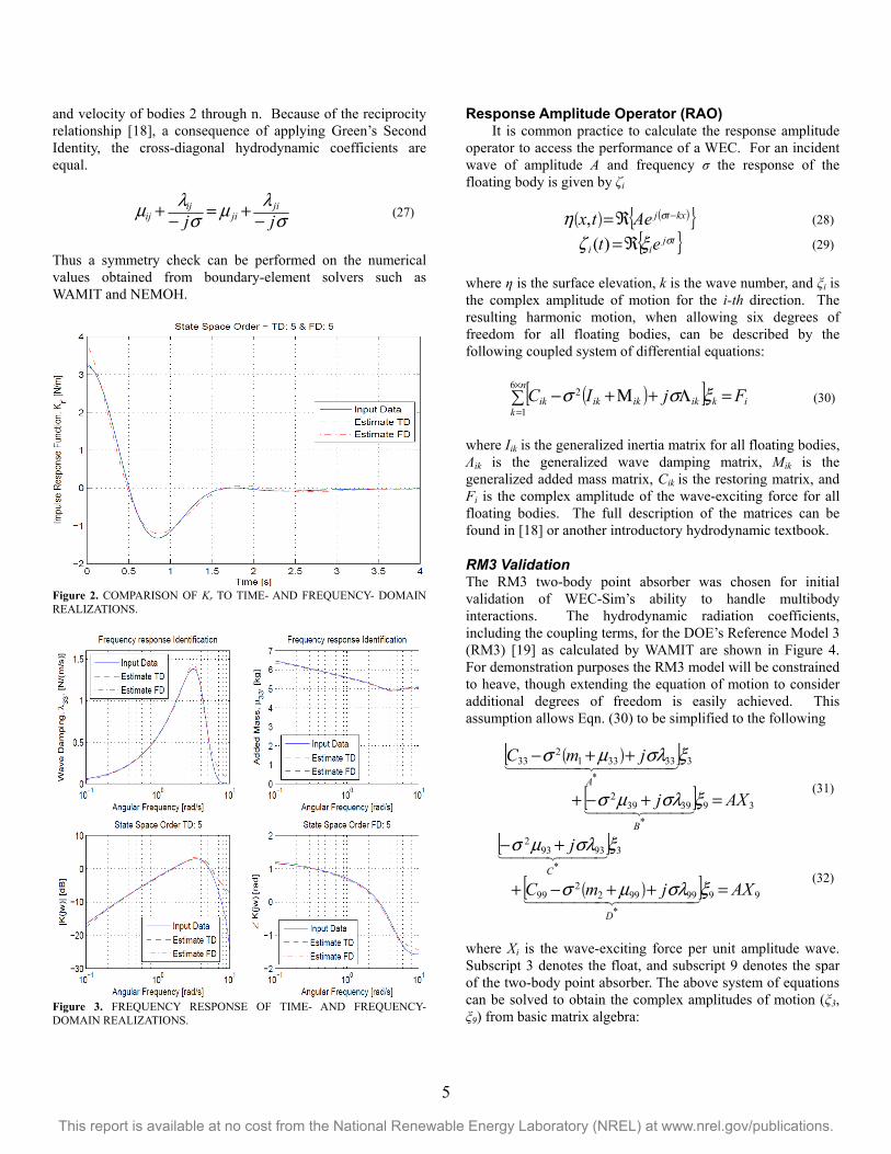
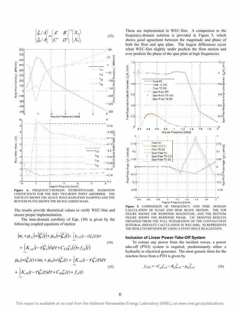
= 1.46 m In this example, an R2 threshold of 0.99 was set and the resulting realizations for the impulse-response function and frequency-dependent radiation coefficients are found in Figure 2 and Figure 3, respectively. In this example, the time-domain characterization outperforms the frequency-domain regression, and the major difference appears in the wave-damping estimation. It was found that the time-domain characterization had better stability than the frequency-domain regression, because it does not require reflection of the unstable poles about the imaginary axis. WEC-Sim users should check the quality of the hydrodynamic data with the custom WEC-Sim MATLAB functions that perform the realizations without running full simulations. These codes allow users to set various fitting parameters using an iterative interface that plots how the fit changes with increasing state-space order. The user can fine tune the input parameters in WEC-Sim to achieve the desired performance.

Figure 1. HEAVE RADIATION COEFFICIENTS FOR GEOMETRY IN TABLE 1.

HYDRODYNAMIC CROSS-COUPLING FORCES For a single floating body, the time-domain representation

of the radiation forces is given by Eqn. (1), because it is dependent only on its own motion. However, most WECs consist of multiple floating bodies that can be in very close proximity, and as a result additional interaction forces arise. These forces are generated as the motion of nearby floating bodies alters the local wave field. Unique to floating-body hydrodynamics are the forces felt by one body because of the motion of “n” additional bodies. This is reflected in the off-diagonal terms of the added mass and wave-damping matrices, which generate a force on Body 1 because of the acceleration

5


and velocity of bodies 2 through n. Because of the reciprocity relationship [18], a consequence of applying Green’s Second Identity, the cross-diagonal hydrodynamic coefficients are equal.

σλμσ

λμjjji

jiij

ij −+=−+ (27)

Thus a symmetry check can be performed on the numerical values obtained from boundary-element solvers such as WAMIT and NEMOH.

Figure 2. COMPARISON OF Kr TO TIME- AND FREQUENCY- DOMAIN REALIZATIONS.

Figure 3. FREQUENCY RESPONSE OF TIME- AND FREQUENCY-DOMAIN REALIZATIONS.

Response Amplitude Operator (RAO) It is common practice to calculate the response amplitude

operator to access the performance of a WEC. For an incident wave of amplitude A and frequency σ the response of the floating body is given by ζi

( ) ( ){ }kxtjAetx −ℜ= ση , (28)

{ }tjii et σξζ ℜ=)( (29)

where η is the surface elevation, k is the wave number, and ξi is the complex amplitude of motion for the i-th direction. The resulting harmonic motion, when allowing six degrees of freedom for all floating bodies, can be described by the following coupled system of differential equations:

( )[ ] =Λ+Μ+−×

=

n

kikikikikik FjIC

6

1

2 ξσσ (30)

where Iik is the generalized inertia matrix for all floating bodies, Λik is the generalized wave damping matrix, Μik is the generalized added mass matrix, Cik is the restoring matrix, and Fi is the complex amplitude of the wave-exciting force for all floating bodies. The full description of the matrices can be found in [18] or another introductory hydrodynamic textbook.

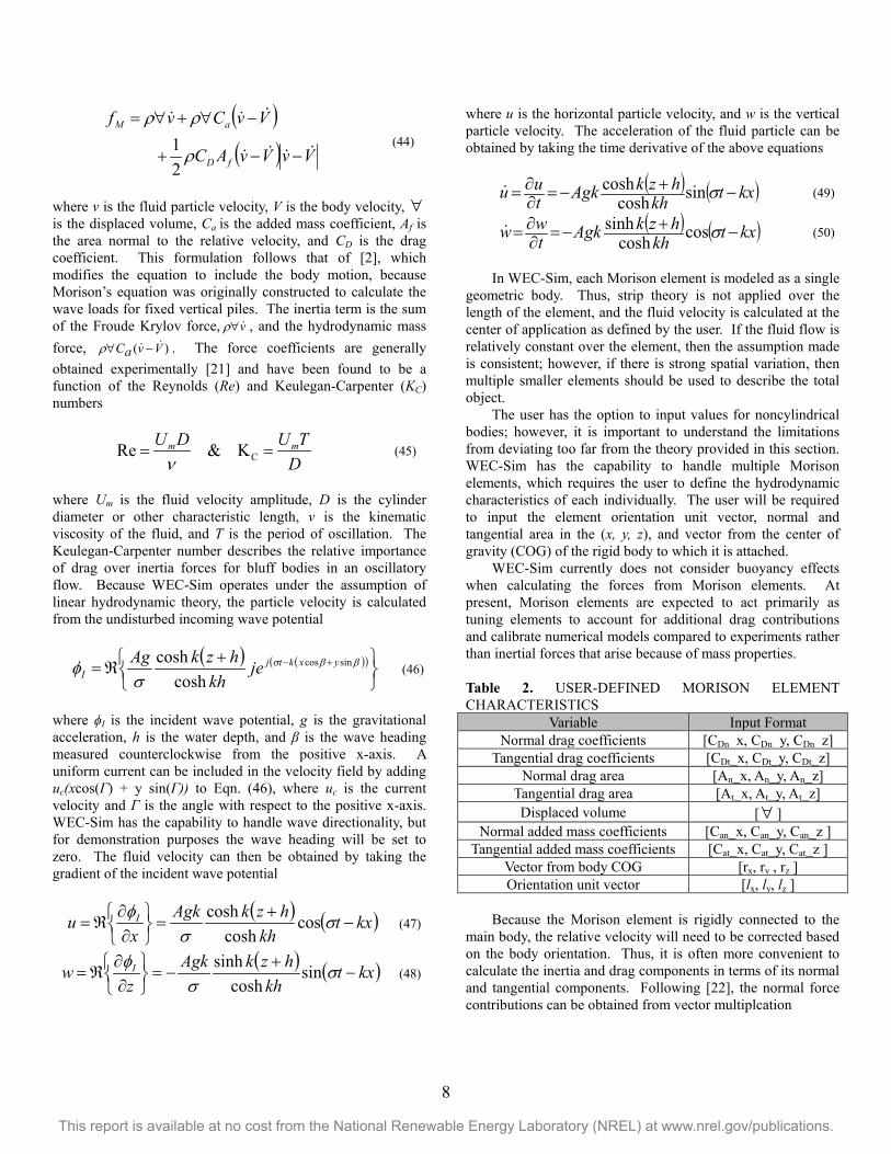
RM3 Validation The RM3 two-body point absorber was chosen for initial validation of WEC-Sim’s ability to handle multibody interactions. The hydrodynamic radiation coefficients, including the coupling terms, for the DOE’s Reference Model 3 (RM3) [19] as calculated by WAMIT are shown in Figure 4. For demonstration purposes the RM3 model will be constrained to heave, though extending the equation of motion to consider additional degrees of freedom is easily achieved. This assumption allows Eqn. (30) to be simplified to the following

( )[ ][ ] 39

*

39392

3

*

333312

33

AXj

jmC

B

A

=+−+

++−

ξσλμσ

ξσλμσ

(31)

[ ]( )[ ] 99

*

999922

99

3

*

93932

AXjmC

j

D

C

=++−+

+−

ξσλμσ

ξσλμσ

(32)

where Xi is the wave-exciting force per unit amplitude wave. Subscript 3 denotes the float, and subscript 9 denotes the spar of the two-body point absorber. The above system of equations can be solved to obtain the complex amplitudes of motion (ξ3, ξ9) from basic matrix algebra:

6


−

=9

31

**

**

9

3

/

/

X

X

DC

BA

A

A

ξξ

(33)

Figure 4. FREQUENCY-DOMAIN HYDRODYNAMIC RADIATION COEFFICIENTS FOR THE RM3 TWO-BODY POINT ABSORBER. THE TOP PLOT SHOWS THE HEAVE WAVE RADIATION DAMPING AND THE BOTTOM PLOTS SHOWS THE HEAVE ADDED MASS.

The results provide theoretical values to verify WEC-Sim and ensure proper implementation.

The time-domain corollary of Eqn. (30) is given by the following coupled equations of motion

( )( ) ( ) ( ) ( ) ( ) ( )

( ) ( ) ( ) ( )tftCdtK

ttm

e

dtK

t

r

t

r

3333939

3339393331

=+ −+

∞+∞+

∞−

∞− −+

ζττζτ

ζμζμ ττζτ

(34)

( ) ( ) ( )( ) ( ) ( ) ( )

( ) ( ) ( ) ( )tftCdtK

dtKtmt

e

t

r

t

r

9999999

3939392393

=+ −+

−+∞++∞

∞−

∞−

ζττζτ

ττζτζμζμ

(35)

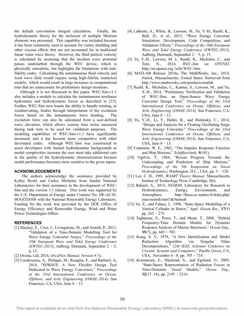
These are implemented in WEC-Sim. A comparison to the frequency-domain solution is provided in Figure 5, which shows good agreement between the magnitude and phase of both the float and spar plate. The largest differences occur when WEC-Sim slightly under predicts the float motion and over predicts the phase of the spar plate at high frequencies.

Figure 5. COMPARISON OF FREQUENCY- AND TIME- DOMAIN CALCULATION OF FLOAT AND SPAR HEAVE MOTION. THE TOP FIGURE SHOWS THE RESPONSE MAGNITUDE, AND THE BOTTOM FIGURE SHOWS THE RESPONSE PHASE. CIC DENOTES RESULTS OBTAINED FROM THE FULL INTEGRATION OF THE CONVOLUTION INTEGRAL (DEFAULT CALCULATION IN WEC-SIM). SS REPRESENTS THE RESULTS OBTAINED BY USING A STATE-SPACE REALIZATION.

Inclusion of Linear Power-Take-Off System To extract any power from the incident waves, a power

take-off (PTO) system is required, predominantly either a hydraulic or electrical generator. The most generic form for the reaction force from a PTO is given by

relgrelgrelgPTO BCf ζμζζ −−−= (36)

7


where ζrel is the relative motion between the floating bodies. The generator spring, damping, and inertia force coefficients are given by Cg, Bg, and μg, respectively. The force applied to each body by the PTO will have the same magnitude, but act in the opposite directions. In the frequency domain, adding the PTO force contribution to Eqn. (30), while zeroing μg, gives

( )[ ] [ ]{ }[ ] 393939

3333312

33

2 AXBjC

BjmCC

gg

gg

=

−+

−−+

+++−+

ξλσμσ

ξλσμσ (37)

[ ] [ ]{ } [{( )] [ ]} 9999992

2

99393932

AXBjm

CCBjC

g

ggg

=+++−

++−+−−

ξλσμσ

ξλσμσ (38)

As described previously, this can be solved to obtain the response amplitude operator and phase of the coupled system. The power absorbed by the PTO is given by:

relrelgrelgrelrelgrelPTO BCfP ζζμζζζζ ++=−= 2 (39)

However, both the relative motion and acceleration are out of phase by π/2 with relative velocity, which results in a time-averaged product of zero. Because the analysis is being completed in the frequency-domain, it is possible to calculate the time-averaged power over one wave period as

( ) ==T

rgrelgTAP

BdttB

TP

0

222

2

1 ζσζ (40)

( )9393

2

9

2

3 cos2 θθξξξξζ −−+=r

(41)

The time-domain corollary of Eqn. (37) and (38) is given by the following coupled equations

( )( ) ( ) ( ) ( )

( ) ( ) ( ) ( )

( ) ( ) ( ) ( ) ( )tftCtCCtB

dtKdtK

tBttm

eggg

t

r

t

r

g

193339

939333

39393331 )(

=−++−

−+ −+

+∞+∞+

∞−∞−

ζζζ

ττζτττζτ

ζζμζμ

(42)

( ) ( ) ( )( ) ( ) ( )

( ) ( ) ( ) ( )

( ) ( ) ( ) ( )tftCCtCtB

dtKdtK

tBtmt

eggg

t

r

t

r

g

299939

999393

39392393

)( =++−+

−+ −+

−∞++∞

∞−∞−

ζζζ

ττζτττζτ

ζζμζμ

(43)

This is implemented in WEC-Sim. Comparisons of the time-domain solution to the frequency-domain solution are provided in Figure 6 and Figure 7.

Figure 6. COMPARISON OF TIME AVERAGED POWER FROM FREQUENCY-AND TIME-DOMAIN SOLUTIONS WHERE Bg = 103 KN/(M/S) AND Cg = 0 N/M.

Figure 7. FREQUENCY- AND TIME-DOMAIN COMPARISON OF THE MAGNITUDE AND PHASE OF THE RELATIVE HEAVE MOTION.

IMPLEMENTATION OF MORISON ELEMENTS The fluid forces in an oscillating flow on a structure of

slender cylinders or other similar geometries arise partly from pressure effects from potential flow and partly from viscous effects. A slender cylinder implies that the diameter, D, is small relative to the wave length, λw, which is generally met when D/λw < 0.1 − 0.2. If this condition is not met, wave diffraction effects must be taken into account. Assuming that the geometries are slender the resulting force can be approximated by a modified Morison formulation [20]

8


( )( ) VvVvAC

VvCvf

fD

aM

−−+

−∀+∀=

ρ

ρρ

21 (44)

where v is the fluid particle velocity, V is the body velocity, ∀ is the displaced volume, Ca is the added mass coefficient, Af is the area normal to the relative velocity, and CD is the drag coefficient. This formulation follows that of [2], which modifies the equation to include the body motion, because Morison’s equation was originally constructed to calculate the wave loads for fixed vertical piles. The inertia term is the sum of the Froude Krylov force, v∀ρ , and the hydrodynamic mass force, )( VvaC −∀ρ . The force coefficients are generally obtained experimentally [21] and have been found to be a function of the Reynolds (Re) and Keulegan-Carpenter (KC) numbers

DTUDU mm == CK&Re

ν (45)

where Um is the fluid velocity amplitude, D is the cylinder diameter or other characteristic length, ν is the kinematic viscosity of the fluid, and T is the period of oscillation. The Keulegan-Carpenter number describes the relative importance of drag over inertia forces for bluff bodies in an oscillatory flow. Because WEC-Sim operates under the assumption of linear hydrodynamic theory, the particle velocity is calculated from the undisturbed incoming wave potential

( ) ( )( )

+

ℜ= +− ββs

sφ sincos

coshcosh yxktj

I jekh

hzkAg (46)

where ϕI is the incident wave potential, g is the gravitational acceleration, h is the water depth, and β is the wave heading measured counterclockwise from the positive x-axis. A uniform current can be included in the velocity field by adding uc(xcos(Γ) + y sin(Γ)) to Eqn. (46), where uc is the current velocity and Γ is the angle with respect to the positive x-axis. WEC-Sim has the capability to handle wave directionality, but for demonstration purposes the wave heading will be set to zero. The fluid velocity can then be obtained by taking the gradient of the incident wave potential

( ) ( )kxtkh

hzkAgkx

u I −+

=

∂∂

ℜ= ss

φ coscosh

cosh (47)

( ) ( )kxtkh

hzkAgkz

w I −+

−=

∂∂

ℜ= ss

φ sincosh

sinh (48)

where u is the horizontal particle velocity, and w is the vertical particle velocity. The acceleration of the fluid particle can be obtained by taking the time derivative of the above equations

( ) ( )kxtkhhzkAgkt

uu −+−=∂∂= ssincosh

cosh (49)

( ) ( )kxtkhhzkAgkt

ww −+−=∂∂= scoscosh

sinh (50)

In WEC-Sim, each Morison element is modeled as a single

geometric body. Thus, strip theory is not applied over the length of the element, and the fluid velocity is calculated at the center of application as defined by the user. If the fluid flow is relatively constant over the element, then the assumption made is consistent; however, if there is strong spatial variation, then multiple smaller elements should be used to describe the total object.

The user has the option to input values for noncylindrical bodies; however, it is important to understand the limitations from deviating too far from the theory provided in this section. WEC-Sim has the capability to handle multiple Morison elements, which requires the user to define the hydrodynamic characteristics of each individually. The user will be required to input the element orientation unit vector, normal and tangential area in the (x, y, z), and vector from the center of gravity (COG) of the rigid body to which it is attached.

WEC-Sim currently does not consider buoyancy effects when calculating the forces from Morison elements. At present, Morison elements are expected to act primarily as tuning elements to account for additional drag contributions and calibrate numerical models compared to experiments rather than inertial forces that arise because of mass properties.

Table 2. USER-DEFINED MORISON ELEMENT CHARACTERISTICS

Variable Input Format Normal drag coefficients [CDn_x, CDn_y, CDn_z]

Tangential drag coefficients [CDt_x, CDt_y, CDt_z] Normal drag area [An_x, An_y, An_z]

Tangential drag area [At_x, At_y, At_z] Displaced volume [∀ ]

Normal added mass coefficients [Can_x, Can_y, Can_z ] Tangential added mass coefficients [Cat_x, Cat_y, Cat_z ]

Vector from body COG [rx, ry , rz ] Orientation unit vector [lx, ly, lz ]

Because the Morison element is rigidly connected to the

main body, the relative velocity will need to be corrected based on the body orientation. Thus, it is often more convenient to calculate the inertia and drag components in terms of its normal and tangential components. Following [22], the normal force contributions can be obtained from vector multiplcation

9


( )lVlCF ranIn ××∀= ρ (51)

( )lVllVlCAF rrDnnDn ××××= ρ2

1 (52)

where Vr is the relative velocity vector, ║·║ is the vector magnitude, × is the cross product (rather than multiplication), and l is the orientation unit vector describing the placement of the element relative to the global coordinate system. For example, an cylinder placed at 45 degrees in the y-z plane would have an orientation unit vector of l = 0 i + √2/2 j + √2/2 z. After the normal relative velocity has been obtained, the tangential component can be obtained from simple subtraction.

Application to Cylindrical Morison Element A simple test case was chosen to demonstrate the correct

implementation of Morison elements within WEC-Sim. The selected geometry, a slender cylinder with a diameter of 0.5 m and length of 20 m, was placed horizontally along the y-axis (l = 0i + 1j + 0k), centered at the origin (0, 0, 0), and the hydrodynamic coefficients were chosen such that 100=∀= annDn CAC . The Morison element was rigidly

connected to a generic floating body, which was fixed in place and impinged upon by a regular wave train propagating along the x-axis. Because the element is fixed, it is possible to perform the vector multiplication in Eqns. (51) and (52), which leads to

( ) ][ costanhsin1 ktkhitCAgkF anIn σσρ ++∀−= � (53)

[ ][ ]ktkhitkh

tkht

AgkCAF Dnn

Dn

σσσσ

σρ

sinsinhcoscosh

sintanhcos

2222

2

−+

=

(54)

A comparison among the above expressions and the output

from WEC-Sim is given in the top plot of Figure 8. The results are an exact match, which verifies the implementation of the fixed condition. The next simulation used the same wave conditions, but the floating body was allowed to heave. The position, velocity, and acceleration outputs from WEC-Sim were used as inputs to Eqns. (51) and (52) to verify the WEC-Sim calculations. The results are shown in the bottom plot in Figure 8, which again agrees and a reduction in the heave force is observed as the relative motion between the body motion and fluid particles are taken into account.

CONCLUSION The work presented in this paper highlights three of the

main modeling capabilities included in the most recent WEC-Sim-v1.1 release. This includes conversion of the fluid memory kernel to state-space form. Simulations showed that

over the operating range of frequencies the state-space representation was able to adequately reproduce the hydrodynamic radiation coefficients; however, a relatively high R2 may need to be set. Because many WECs consist of two or more excited bodies, the ability to model the body-to-body hydrodynamics was included in WEC-Sim. This is an important feature to consider during the design process, because the effects can lead to reduced floater motion and thereby decrease annual energy production.

Figure 8. COMPARISON AMONG THE MORISON FORCES CALCULATED BY WEC-SIM AND THEORETICAL VALUES. IN THE TOP FIGURE THE FLOATING BODY POSITION WAS FIXED, WHEREAS IN THE BOTTOM FIGURE THE FLOATING BODY WAS ALLOWED TO HEAVE. THE WAVE ELEVATION WAS SCALED BY 100 FOR EASIER VIEWING.

Combined with the state-space representation, significant reductions in computational time were observed compared to

10


the default convolution integral calculation. Finally, the hydrodynamic theory for the inclusion of multiple Morison elements was presented. This capability was included because it has been commonly used to account for vortex shedding and other viscous effects that are not accounted for in traditional linear water wave theory. However, the fluid particle velocity is calculated by assuming that the incident wave potential passes undisturbed through the WEC device, which is physically unrealistic, but highlights the limitations with mid-fidelity codes. Calculating the instantaneous fluid velocity and local wave field would require using high-fidelity numerical models, which would result in large increases in computational time that are unnecessary for preliminary design iterations. Although it is not discussed in this paper, WEC-Sim-v1.1 also includes a module to calculate the instantaneous nonlinear hydrostatic and hydrodynamic forces as described in [23]. Further, WEC-Sim now boasts the ability to handle rotating, or weathervaning, bodies through interpolation of the excitation forces based on the instantaneous wave heading. The excitation force can also be calculated from a user-defined wave elevation, which allows custom time series measured during tank tests to be used for validation purposes. The modeling capabilities of WEC-Sim-v1.1 have significantly increased, and it has become more competitive with other developed codes. Although WEC-Sim was constructed to assist developers with limited hydrodynamic backgrounds as model complexities increase the user must take additional care in the quality of the hydrodynamic characterization because model performance becomes more sensitive to the given inputs.

ACKNOWLEDGEMENTS The authors acknowledge the assistance provided by

Kelley Reuhl and Carlos Michelen from Sandia National Laboratories for their assistance in the development of WEC-Sim and the version 1.1 release. This work was supported by the U.S. Department of Energy under Contract No. DE-AC36-083GO28308 with the National Renewable Energy Laboratory. Funding for the work was provided by the DOE Office of Energy Efficiency and Renewable Energy, Wind and Water Power Technologies Office.

REFERENCES [1] Mackay, E., Cruz, J., Livingstone, M., and Arnold, P., 2013,

“Validation of a Time-Domain Modelling Tool for Wave Energy Converter Arrays,” Proceedings of the 10th European Wave and Tidal Energy Conference (EWTEC-2013), Aalborg, Denmark, September 2 − 5, p. 12.

[2] Orcina, Ltd, 2014, OrcaFlex Manual, Version 9.7a. [3] Combourieu, A., Philippe, M., Rongère, F., and Barbarit, A,

2014, “INWAVE: A New Flexible Design Tool Dedicated to Wave Energy Converters,” Proceedings of the 33rd International Conference on Ocean, Offshore, and Artic Engineering (OMAE-2014), San Francisco, CA, USA, June 8 − 13.

[4] LaBonte, A., White, B., Lawson, M., Yu, Y.-H., Ruehl, K., Bull, D., et al., 2013, “Wave Energy Converter Simulation: Development, Code Competition, and Validation Efforts,” Proceedings of the 10th European Wave and Tidal Energy Conference (EWTEC-2013), Aalborg, Denmark, September 2 − 5, p. 15.

[5] Yu, Y.-H., Lawson, M. J., Ruehl, K., Michelen, C., and Tom, N., 2014, WEC-Sim on OPENEI, http://en.openei.org /wiki/WEC-Sim.

[6] MATLAB Release 2014a, The MathWorks, Inc., 2014, Natick, Massachusetts, United States. Retrieved from http://www.mathworks.com/products/matlab.

[7] Ruehl, K., Michelen, C., Kanner, S., Lawson, M., and Yu, Y.-H., 2014, “Preliminary Verification and Validation of WEC-Sim, an Open-Source Wave Energy Converter Design Tool,” Proccedings of the 33rd International Conference on Ocean, Offshore, and Artic Engineering (OMAE-2014), San Francisco, CA, USA, June 8 − 13.

[8] Yu, Y.-H., Li, Y., Hallet, K., and Hotimsky, C., 2014, “Design and Analysis for a Floating Oscillating Surge Wave Energy Converter,” Proccedings of the 33rd International Conference on Ocean, Offshore, and Artic Engineering (OMAE-2014), San Francisco, CA, USA, June 8 − 13.

[9] Cummins, W. E., 1962, “The Impulse Response Function and Ship Motions,” Schiffstechnik, 9(101).

[10] Ogilvie, T., 1964, “Recent Progress Towards the Understading and Prediction of Ship Motions,” Proceedings of the 5th Symposium on Naval Hydrodynamics, Washington, D.C., USA, pp. 3 − 128.

[11] Lee, C. H., 1995, WAMIT Theory Manual. Massachusetts Institue of Technology Press, Cambridge, MA.

[12] Babarit, A., 2014, NEMOH, Laboratory for Research in Hydrodynamics, Energy, Environment, and Atmosphere, http://lheea.ec-nantes.fr/doku.php/ emo/nemoh/start?&#nemoh

[13] Yu, Z., and Falnes, J., 1996, “State-Space Modelling of a Vertical Cylinder in Heave,” Appl. Ocean Res., 17(5) pp. 265 − 275.

[14] Taghipour, E., Perez, T., and Moan, T., 2008, “Hybrid Frequency-Time Domain Models for Dynamic Response Analysis of Marine Structures,” Ocean Eng., 35(7), pp. 685 − 705.

[15] Kung, S. Y., 1978, “A New Identification and Model Reduction Algorithm via Singular Value Decompositions,” 12th IEEE Asilomar Conferece on Circuits, Systems and Computers,” Pacific Grove, CA, USA, November 6 - 8, pp. 705 − 714.

[16] Kristiansen, E., Hijulstad, A., and Egeland, O., 2005, “State-Space Representation of Radiation Forces in Time-Domainn Vessel Models,” Ocean Eng., 32(17−18), pp. 2195 − 2216.

11


[17] Yeung, R. W., 1981, “Added Mass and Damping of a Vertical Cylinder in Finite-depth Waters,” Appl. Ocean. Res., 3(3), pp. 119 − 133.

[18] Newman, J. H., 1977, Marine Hydrodynamics. Massachusetts Institute of Technology Press, Cambridge, MA.

[19] Neary, V., Previsic, M., Jepsen, R. A., Lawson, M. J., Yu, Y. -H., Copping, A. E., et al., 2014, Methodology for Design and Economic Analysis of Marine Energy Conversion (MEC) Technologies, SAND2014-9040-RMP, Sandia National Laboratories, Albuquerque, NM.

[20] Morison, J. R., Johnson, J. W., and Schaaf, S. A., 1950, “The Force Exerted by Surface Waves on Piles,” Journal of Petroleum Technology, 2(5), pp. 149 − 154.

[21] Keulegan, G. H. and Carpenter, L. H., 1958, “Forces on Cylinders and Plates in an Oscillating Fluid,” Journal of the National Bureau of Standards, 60(5), pp. 423 − 440.

[22] Gran, S., 1992, A Course in Ocean Engineering. In Developments in Marine Technology, Amsterdam - London-New York-Tokyo, Elsevier Science Publishers, Vol. 8, pp. 295 − 300.

[23] Lawson, M., Yu, Y.-H., Nelessen, A., Ruehl, K., and Michelen, C., 2014, “Implementing Nonlinear Buoyancy and Excitation Forces in the WEC-SIM Wave Energy Converter Modeling Tool,” Proccedings of the 33rd International Conference on Ocean, Offshore, and Artic Engineering (OMAE-2014), San Francisco, CA, USA, June 8 − 13.

demonstration of the recent additions in modeling

Documents