demystifying the lucas-kanade optical flow algorithm · pdf filedemystifying the lucas-kanade...
TRANSCRIPT
XAPP1300 (v1.0) February 3, 2017 1www.xilinx.com
SummaryThe Lucas-Kanade (LK) algorithm for dense optical flow estimation is a widely known and adopted technique for object detection and tracking in image processing applications. This algorithm is computationally intensive and its implementation in an FPGA is challenging from both a design and a performance perspective. This application note describes how to implement the LK algorithm with the Xilinx Vivado® High-level Synthesis (HLS) tool to achieve real-time performance in the Zynq®-7000 All Programmable (AP) SoC without image quality degradation.
A real-time demonstration on a Zynq-7000 AP SoC reference board was built with the SDSoC™ development environment's integrated tool. The design reads video data from a file and writes back the processed data to a file, instead of reading and writing frame buffers. The design was created in less than eight weeks by an engineer. This application note also serves as a tutorial demonstrating good C/C++ coding techniques for obtaining the best performance from Vivado HLS in image processing. Download the reference design files for this application note from the Xilinx website. For detailed information about the design files, see Reference Design.
IntroductionOptical flow is a family of techniques used to estimate the pattern of the apparent motion of image objects caused by the movement of objects or a camera in a video sequence. It is a vector field where each vector has two components to show the displacement between points due to their movement from the first image (also called frame) to the second image. In image processing and computer vision, the LK algorithm is a popular method for optical flow [Ref 1]. This algorithm assumes that the flow is essentially constant in the local neighborhood of the pixel under consideration, and solves the basic optical flow equations for all of the pixels in that neighborhood with the least squares criterion. A method that computes the optical flow for some pixels in the image is referred to as sparse, while dense techniques process all of the pixels.
The LK algorithm is no longer considered state-of-the-art, but it is still used as a reference in most scientific papers because of the numerous public domain implementations in different programming languages (such as, OpenCV, Python, MATLAB® software, and OpenCL™ framework). The LK algorithm is very complicated, and its implementation in an FPGA has been considered almost impossible without a huge time investment. This application note shows that it is possible to implement the algorithm in an FPGA. The LK dense optical flow algorithm is modeled in the C/C++ programming language with the proper coding style for achieving the best performance from Vivado HLS. A bottom-up approach is used in the design procedure. The
Application Note: Zynq-7000 AP SoC
XAPP1300 (v1.0) February 3, 2017
Demystifying the Lucas-Kanade Optical Flow Algorithm with Vivado HLSAuthors: Daniele Bagni, Pari Kannan, and Stephen Neuendorffer

Introduction
XAPP1300 (v1.0) February 3, 2017 2www.xilinx.com
optical flow intellectual property (IP) core is implemented with Vivado HLS. The embedded system design is created with the SDSoC environment to implement a real-time demonstrator either on the ZC702 evaluation board or on the ZC706 evaluation board based on file I/O video data. For more information, see ZC702 Evaluation Board for the Zynq-7000 XC7020 All Programmable SoC User Guide (UG850) [Ref 2] and Zynq-7000 All Programmable SoC ZC706 Evaluation Kit Getting Started Guide (UG961) [Ref 3], respectively.
The Xilinx SDSoC is an Eclipse-based integrated development environment (IDE) for implementing heterogeneous embedded systems using the Zynq-7000 AP SoC. The SDSoC environment includes a full-system optimizing C/C++ compiler that provides automated software acceleration in programmable logic combined with automated system connectivity generation. An application is written as C/C++ code with the programmer identifying a target platform and a subset of the functions within the application to be compiled into hardware. The SDSoC system compiler then compiles the application into hardware and software to realize the complete embedded system implemented on a Zynq-7000 AP SoC, including a complete boot image with firmware, operating system, and application executable. For more information, see SDSoC Environment User Guide (UG1027) [Ref 4].
Vivado HLS is a key component of the SDSoC environment. The Vivado HLS C/C++ compiler generates high-performance pipelined architecture according to the given constraints, and creates test benches to ensure that the behaviors of the HDL and C/C++ code are identical. In many cases, the Vivado HLS synthesized code has similar efficiency and performance to that of hand-coded HDL designed by an experienced hardware engineer. For more information on Vivado HLS, see Vivado Design Suite User Guide: High-Level Synthesis (UG902) [Ref 5].
The C/C++ design becomes an IP core that can be easily customized for new applications by slight modifications to the C header files containing the design parameters (for example image size, number of bits per pixel, dimension of the sliding window, and floating point or fixed point data types).
The design procedure described in this application note applies to Vivado HLS and the SDSoC Vivado 2016.2 and 2016.3 IDE release tools.

Theory of Operation
XAPP1300 (v1.0) February 3, 2017 3www.xilinx.com
Theory of OperationThe C/C++ model of the LK dense optical flow algorithm is based on the mathematical explanations in Pyramidal Implementation of the Affine Lucas Kanade Feature Tracker Description Algorithm, J. Y. Bouguet, Intel Corporation, 2001 [Ref 7] and the MathWorks documentation: opticalFlowLK class [Ref 8], which are summarized in this section.
The optical flow equation is shown in Equation 1. In this equation, (vx, vy) are the two unknown components of the motion vectors in the horizontal and vertical directions, respectively. Ix, Iy, and It are the spatial and temporal image brightness derivatives.
Equation 1
Because one equation with two unknowns cannot be solved, the LK method divides the original image into smaller sections and assumes a constant velocity in each section. It then performs a weighted least-square fit of the optical flow equation to a constant model for (vx, vy) in each section. The method achieves this fit by minimizing Equation 2, in which W is a window function that emphasizes the optical flow constraint equation at the center of each section.
Equation 2
The solution to the minimization problem is shown in Equation 3.
Equation 3
This equation can be solved because it is a system of two equations with two unknowns.
Figure 1 illustrates the basic functions of the LK method working on two images I1(x, y) and I2(x, y) within the same video sequence. The process includes these stages:
1. Both input images are smoothed by a noise reduction filter of size 5x5 (3x3 or 7x7 are also valid algorithm design options). This stage reduces the image noise and prevents this noise from being amplified by the second stage.
2. The spatial derivatives Ix Iy are computed with a filter of size 5x5 (3x3 or 7x7 are also valid options). The temporal derivative It is the difference between the two input images, properly delayed by a 5x5 unitary filter to be aligned with the spatial derivatives.
3. The five parameters of Equation 3 are computed by accumulation on a squared window W of size NxN (with N=7, …, 53) (called integration window in this application note).
4. The vector components vx and vy are computed by inverting the 2x2 real and symmetric matrix of Equation 3 from the previous stage.
Ixvx Iyvy It+ + 0=
ΣW2 Ixvx Iyvy It+ +[ ]2 0=
ΣW2Ix2 ΣW2IxIy
ΣW2IxIy ΣW2Iy2
vx
vy– ΣW2IxIt
ΣW2IyIt
=

Theory of Operation
XAPP1300 (v1.0) February 3, 2017 4www.xilinx.com
After the motion vectors are computed, image I1 can be reconstructed from image I2 with Equation 4, which is referred to as motion compensation.
Equation 4
With an ideally perfect optical flow field, it is:
Equation 5
In reality, the worse the computed optical flow is, the more distortions will appear in the motion compensated image. For example, the computed optical flow deteriorates when there are occlusion areas in the image or in indoor scenes with many reflective floors and walls. In the LK optical flow method, the integration window size dictates the integrity of the motion vectors. The larger the window, the better the quality of the motion compensated image.
As an example, Figure 2, Figure 3, Figure 4, and Figure 5, respectively, illustrate the two input images and the motion compensated images obtained with either an 11x11 or a 43x43 integration window size. In the second input (Figure 3), the difference from the first input is that the car in the left lane of incoming traffic has moved slightly forward (in the normal direction of traffic), and this is the information that needs to be detected. The image quality is much better in Figure 5 than in Figure 4.
X-Ref Target - Figure 1
Figure 1: Block Diagram of Lucas-Kanade Dense Optical Flow
Smooth 5x5
Smooth 5x5
Ix5x5
Iy5x5
It5x5
Compute Integralson a N x N
window size
Compute Vectors
(with 2x2 matrix inversion)
Dense optical flow
Block 4: ComputeVectors
I1
I2
Block 1: twoIsotropicFilters()
Block 3: ComputeIntegrals()
Block 2: SpatialTemporalDerivatives()X18179-012017
I1MC x y,( ) I2 x vx+ y vy+,( )=
I1MC x y,( ) I1 x y,( )≈

Theory of Operation
XAPP1300 (v1.0) February 3, 2017 5www.xilinx.com
X-Ref Target - Figure 2
Figure 2: Input Image I1
X18059-110116
X-Ref Target - Figure 3
Figure 3: Input Image I2
X18060-110116

Theory of Operation
XAPP1300 (v1.0) February 3, 2017 6www.xilinx.com
X-Ref Target - Figure 4
Figure 4: Motion Compensated Image with an Integration Window Size of 11x11
X18061-012317
X-Ref Target - Figure 5
Figure 5: Motion Compensated Image with an Integration Window Size of 43x43
X18062-012317

Theory of Operation
XAPP1300 (v1.0) February 3, 2017 7www.xilinx.com
Motion vectors coded as colors are shown in Figure 6 and Figure 7. These figures illustrate the optical flow when computed with an integration window size of 11x11 or 43x43, respectively. The optical flow appears smoother and more coherent with a larger integration window.
X-Ref Target - Figure 6
Figure 6: Motion Vectors Generated via a 11x11 Integration Window
X18063-110116

Theory of Operation
XAPP1300 (v1.0) February 3, 2017 8www.xilinx.com
X-Ref Target - Figure 7
Figure 7: Motion Vectors Generated via a 43x43 Integration Window
X18064-110116

Theory of Operation
XAPP1300 (v1.0) February 3, 2017 9www.xilinx.com
The motion vectors computed by the fourth stage can have non-integer values. Consequently, they are at subpixel accuracy and must be interpolated. Most of the optical flow methods available in literature apply the bilinear interpolation for sub-pixel accuracy, as shown in Figure 8 [Ref 9]. The red points are pixels at integer coordinates x1, y1, x2, y2 with luminance values Q11 Q12, Q21, and Q22. The green and blue points are sub-pixel coordinates with luminance values R1, R2, and P. This MATLAB pseudo-code fragment explains the bilinear interpolation:
x1 = floor(x); y = floor(y); kx = x-x1; ky = y-y1;
R1 = Q11 * (1- kx) + kx * Q21; R2 = Q12 * (1- kx) + kx * Q22;
P = R1 * (1- ky) + ky * R2;
X-Ref Target - Figure 8
Figure 8: Subpixel Bilinear Interpolation
X18180-012017

C++ Model for HLS
XAPP1300 (v1.0) February 3, 2017 10www.xilinx.com
C++ Model for HLSThe efficient implementation of image processing algorithms on Xilinx FPGAs with Vivado HLS requires proper coding style in the C/C++ language. In software, images are 2D arrays that reside in memory. In FPGA hardware, images are a stream of pixels coming in a raster scan order (from top-left to bottom-right) that cannot be stored completely in the FPGA internal memory. Typically, only a few image lines are stored in the line buffers that delay the incoming stream by a factor of the line width. Vivado HLS maps these line buffers as FIFOs implemented into dual-port block RAM elements (one block RAM can be configured to store 1024 pixels up to 18 bits per pixel).
Figure 9 shows the architecture of a 2D convolution filter with a 3x3 kernel size, which requires two line buffers (the third line is the incoming stream itself) and a sliding window of size 3x3. In image processing terminology, kernel refers to the 2D filter coefficients area (not necessarily a squared shape). Sliding window refers to the input pixels neighborhood that is weighted and summed by the coefficients of the filter kernel to produce each output pixel. The center of the window slides around the output pixel to be generated in raster scan order. The kernel (and shape) size dictates the window size (and shape) of the 2D filter. The larger the window size N, the more line buffers are required. In image processing, 2D convolutional filters do not usually go beyond N=16. Furthermore, a line buffer requires simultaneous read and write access, which takes full advantage of the dual-port nature of block RAMs. Conversely, the sliding window is implemented as parallel registers. For more information on efficiently implementing memory structures for image processing in Vivado HLS, see Vivado Design Suite User Guide: High-Level Synthesis (UG902) [Ref 5].
X-Ref Target - Figure 9
Figure 9: Line Buffers and 3x3 Sliding Window Architecture
= Register
3x3 sliding window
Filter Kernel
Line buffer
Line buffer
Pixel Stream
X18181-120216

C++ Model for HLS
XAPP1300 (v1.0) February 3, 2017 11www.xilinx.com
HLS Efficient Implementation of 2D Convolution Filter in C/C++
The previous concepts are applied to the C/C++ code listed here, which is the basis of all the routines implementing the LK dense optical flow design.
void hls_2DFilter(pix_t inp_img[MAX_HEIGHT*MAX_WIDTH], pix_t out_img[MAX_HEIGHT*MAX_WIDTH], short int height, short int width) {short int row, col; pix_t filt_out;
pix_t window[FILTER_SIZE][FILTER_SIZE]; // sliding window#pragma HLS ARRAY_PARTITION variable=window complete dim=0
pix_t right_col[FILTER_SIZE]; // right-most, incoming columnstatic pix_t line_buffer[FILTER_SIZE][MAX_WIDTH]; // line-buffers#pragma HLS ARRAY_PARTITION variable=line_buffer complete dim=1
// effective filtering 2D loopL1: for(row = 0; row < height+FILTER_OFFS; row++){L2: for(col = 0; col < width+FILTER_OFFS; col++){#pragma HLS PIPELINE II=1 // line-buffer fillif(col < width)
for(unsigned char ii = 0; ii < FILTER_SIZE-1; ii++){
right_col[ii]=line_buffer[ii][col]=line_buffer[ii+1][col];}
if((col < width) && (row < height)){
pix_t pix = inp_img[row*MAX_WIDTH+col];right_col[FILTER_SIZE-1] = line_buffer[FILTER_SIZE-1][col] = pix;
}
//Shift from left to right the sliding window to make room for the new columnfor(unsigned char ii = 0; ii < FILTER_SIZE; ii++)
for(unsigned char jj = 0; jj < FILTER_SIZE-1; jj++)window[ii][jj] = window[ii][jj+1];
for(unsigned char ii = 0; ii < FILTER_SIZE; ii++)window[ii][FILTER_SIZE-1] = right_col[ii];
//This design assumes there are no edges on the boundary of the imageif ( (row>=FILTER_OFFS) & (col>=FILTER_OFFS) & (row<height) & (col<width) )
filt_out = filter_kernel_operator(window);else
filt_out = 0;
if ( (row>=FILTER_OFFS) & (col>=FILTER_OFFS) & (row<height) & (col<width) )out_img[(row-FILTER_OFFS)*MAX_WIDTH+(col-FILTER_OFFS)] = (filt_out);
} // end of L2} // end of L1
} // end of function

C++ Model for HLS
XAPP1300 (v1.0) February 3, 2017 12www.xilinx.com
• MAX_WIDTH and MAX_LINES are the image resolution in terms of columns and lines.
• The sliding window is a 2D squared array window of size FILTER_SIZE partitioned into separate registers via the ARRAY_PARTITION dim=0 HLS directive.
• The line buffer is a 2D rectangular array that contains FILTER_SIZE lines of MAX_WIDTH pixels per line partitioned into FILTER_SIZE separate block RAMs via the ARRAY_PARTITION dim=1 HLS directive, so that each image line is stored in its own dual-port block RAM.
Note: The Vivado HLS compiler implements only FILTER_SIZE-1 lines in the hardware design, even if the C/C++ code clearly applies FILTER_SIZE lines for better readability and ease of programming.
• This processing style introduces a vertical and horizontal delay of FILTER_OFFS lines and FILTER_OFFS pixels, respectively, between the input image and the output image (besides the processing delay needed for all the remaining operations). This requires that the L1 and L2 FOR loops be extended by the same amount beyond the image resolution values because the first and last FILTER_OFFS columns and lines of the output image are filled with zero values (more sophisticated image processing would extend the input image resolution with mirroring to avoid these zero values, but this is not necessary for this application note, and it can be easily implemented into the C/C++ model).
• While filling the line buffer, the rightmost incoming column of input pixels is stored in the 1D array right_col and then used to update the 2D array window column by column from right (index jj+1) to left (index jj) to emulate the sliding shift from left to right.
hls_twoIsotropicFilters()This routine smoothly filters the two input images with a 2D 5x5 kernel via the innermost hls_isotropic_kernel() subroutine. Its structure is the same as listed in HLS Efficient Implementation of 2D Convolution Filter in C/C++. The main difference is the code style adopted to save around 50% of the theoretically needed block RAM. Assuming 12 BITS_PER_PIXEL and 1920 MAX_WIDTH pixels per line so that an entire image line can be stored in two block RAM elements, 8 block RAMs are needed to store four lines of image I1 and 8 block RAMs are needed for image I2 (16 block RAMs total). Because the Xilinx block RAM has a maximum width of 18 bits if configured with a 1024 word depth, 25% of the block RAM is saved by packing the two 12-bit pixels into a 24-bit word. Consequently, the total amount of block RAM is 12 instead of 16 for the filtering of the two input images.
Packing of the two 12-bit pixels is done via the HLS range operator from the ap_int C++ class of variable size integer data types (the ap_int.h header file must be included), as shown in this C/C++ code fragment.

C++ Model for HLS
XAPP1300 (v1.0) February 3, 2017 13www.xilinx.com
Packing Two Pixels Into a Larger Word With HLS C++ Range Operator
#include "ap_int.h" // HLS arbitrary width integer data typestypedef ap_uint<BITS_PER_PIXEL > pix_t; // input pixeltypedef ap_int<BITS_PER_PIXEL*2> dualpix_t;// to pack 2 pixels
void hls_twoIsotropicFilters( . . . ){unsigned short int row, col;pix_t filt_out1, filt_out2, pix1, pix2;dualpix_t two_pixels;
dualpix_t pixels[FILTER_SIZE]; #pragma HLS ARRAY_PARTITION variable=pixels complete dim=0
dualpix_t window[FILTER_SIZE*FILTER_SIZE];#pragma HLS ARRAY_PARTITION variable=window complete dim=0
static dualpix_t lpf_lines_buffer[FILTER_SIZE][MAX_WIDTH];#pragma HLS ARRAY_PARTITION variable=lpf_lines_buffer complete dim=1
// effective filteringL1: for(row = 0; row < height+FILTER_OFFS; row++)
{#pragma HLS LOOP_TRIPCOUNT min=hls_MIN_H max=hls_MAX_HL2: for(col = 0; col < width+FILTER_OFFS; col++)
{#pragma HLS PIPELINE#pragma HLS LOOP_TRIPCOUNT min=hls_MIN_W max=hls_MAX_W
// Line Buffer fillif(col < width)for(unsigned char ii = 0; ii < FILTER_SIZE-1; ii++)
{ pixels[ii]=lpf_lines_buffer[ii][col]= lpf_lines_buffer[ii+1][col]; }
//There is an offset to accomodate the active pixel regionif((col < width) && (row < height)){
pix1 = (pix_t) inp1_img[row*MAX_WIDTH+col];pix2 = (pix_t) inp2_img[row*MAX_WIDTH+col];two_pixels.range(2*BITS_PER_PIXEL-1, BITS_PER_PIXEL) = pix2;two_pixels.range( BITS_PER_PIXEL-1, 0) = pix1;pixels[FILTER_SIZE-1]=lpf_lines_buffer[FILTER_SIZE-1][col]=two_pixels;
}
//Shift right the processing window to make room for the new columnL3:for(unsigned char ii = 0; ii < FILTER_SIZE; ii++)
L4:for(unsigned char jj = 0; jj < FILTER_SIZE-1; jj++){window[ii*FILTER_SIZE+jj]=window[ii*FILTER_SIZE+jj+1];
}L5:for(unsigned char ii = 0; ii < FILTER_SIZE; ii++){
window[ii*FILTER_SIZE+FILTER_SIZE-1] = pixels[ii];}
//This design assumes there are no edges on the boundary of the imageif ((row>=FILTER_OFFS)&(col>=FILTER_OFFS)&(row<height)&(col< width)){
two_pixels = hls_isotropic_kernel(window);filt_out1 = two_pixels.range( BITS_PER_PIXEL-1, 0);filt_out2 = two_pixels.range(2*BITS_PER_PIXEL-1, BITS_PER_PIXEL);
}else { filt_out1 = 0; filt_out2 = 0; }
if ( (row >= FILTER_OFFS) & (col >= FILTER_OFFS)) {

C++ Model for HLS
XAPP1300 (v1.0) February 3, 2017 14www.xilinx.com
out1_img[(row-FILTER_OFFS)*MAX_WIDTH+(col-FILTER_OFFS)] = filt_out1;out2_img[(row-FILTER_OFFS)*MAX_WIDTH+(col-FILTER_OFFS)] = filt_out2;
}
} // end of L2} // end of L1
}
The hls_isotropic_kernel() subroutine performs the 2D convolution, as shown in this C/C++ code fragment. The 5x5 array of coefficients has the values suggested by the MathWorks documentation: opticalFlowLK class [Ref 8].
2D Convolution of hls_isotropic_kernel() Routine C/C++ Code Fragment
const coe_t coeff[FILTER_SIZE][FILTER_SIZE] = {{ 1, 4, 6, 4, 1},{ 4, 16, 24, 16, 4},{ 6, 24, 36, 24, 6},{ 4, 16, 24, 16, 4},{ 1, 4, 6, 4, 1}
};// local variablesint accum1 = 0, accum2 = 0;int normalized_accum1, normalized_accum2;pix_t pix1, pix2, final_val1, final_val2;dualpix_t two_pixels;
//Compute the 2D convolutionL1:for (i = 0; i < FILTER_SIZE; i++) {L2:for (j = 0; j < FILTER_SIZE; j++) { two_pixels = window[i][j];
pix1 = two_pixels.range( BITS_PER_PIXEL-1, 0);pix2 = two_pixels.range(2*BITS_PER_PIXEL-1, BITS_PER_PIXEL);accum1 = accum1 + ((short int) pix1 * (short int) coeff[i][j]);accum2 = accum2 + ((short int) pix2 * (short int) coeff[i][j]);
} // end of L2} // end of L1// do the correct normalization if needednormalized_accum1 = accum1 / 256;normalized_accum2 = accum2 / 256;final_val1 = (pix_t) normalized_accum1;final_val2 = (pix_t) normalized_accum2;
hls_SpatialTemporalDerivatives This routine performs the spatial derivatives Ix and Iy with a 2D convolution kernel size of 5x5. The temporal derivative It is the difference between the two input images. The structure of the code is very similar to the previous routine. For an 8-bit pixel, the derivatives are 9-bit samples. Ix and Iy are packed into an 18-bit larger word, which is then stored into the lines buffer. The hls_derivative_kernel() is the innermost subroutine structure and applies the coefficient values suggested by the MathWorks documentation: opticalFlowLK class [Ref 8], as illustrated in 2D Convolution of hls_derivatives_kernel(). With fixed coefficient kernel sizes, the FPGA resources utilization of twoIsotropicFilters() and SpatialTemporalDerivatives() routines are almost constant, independent of the image resolution. Only the number of block RAMs can change depending on the effective image line width.

C++ Model for HLS
XAPP1300 (v1.0) February 3, 2017 15www.xilinx.com
2D Convolution of hls_derivatives_kernel()
typedef ap_int< BITS_PER_PIXEL+1> flt_t; // for the 3 derivatives
// derivative filter in a 5x5 kernel size: [-1 8 0 -8 1]// coefficients are swapped to get same results as MATLABconst coe_t y_coeff[FILTER_SIZE][FILTER_SIZE] = { { 0, 0, 1, 0, 0},{ 0, 0, -8, 0, 0}, { 0, 0, 0, 0, 0}, { 0, 0, 8, 0, 0}, { 0, 0, -1, 0, 0} }; const coe_t x_coeff[FILTER_SIZE][FILTER_SIZE] = { { 0, 0, 0, 0, 0},{ 0, 0, 0, 0, 0}, { 1, -8, 0, 8, -1}, { 0, 0, 0, 0, 0}, { 0, 0, 0, 0, 0} };
int accum_x = 0, accum_y = 0;dualpix_t two_pix;pix_t pix1, pix2;int normalized_accum_x, normalized_accum_y;flt_t final_val_x, final_val_y, final_val_t;
//Compute the 2D convolutionL1:for (i = 0; i < FILTER_SIZE; i++)
{L2:for (j = 0; j < FILTER_SIZE; j++) {
two_pix = window[i][j]; pix1 = two_pix.range(2*BITS_PER_PIXEL-1, BITS_PER_PIXEL);pix2 = two_pix.range( BITS_PER_PIXEL-1, 0);
signed short int loc_mult_x = ( pix1 * x_coeff[i][j]); accum_x = accum_x + loc_mult_x;signed short int loc_mult_y = ( pix1 * y_coeff[i][j]); accum_y = accum_y + loc_mult_y;
if ( (i==2)&(j==2) )final_val_t = pix2 - pix1; //central pix is window[2][2]
} // end of L2} // end of L1
// do the correct normalizationnormalized_accum_x = accum_x / 12;normalized_accum_y = accum_y / 12;final_val_x = (flt_t) normalized_accum_x;final_val_y = (flt_t) normalized_accum_y;Ix = final_val_x;Iy = final_val_y;
It = final_val_t;

C++ Model for HLS
XAPP1300 (v1.0) February 3, 2017 16www.xilinx.com
hls_ComputeIntegrals() This module computes the five parameters of Equation 3, rewritten here to match more closely the names of C/C++ code variables by integrating the squared values of the partial derivatives within a window of size NxN, with N=7, …, 53.
Equation 6
This is the most critical routine in terms of FPGA resources. An NxN integration window size module requires N–1 lines to be buffered (each line consuming two block RAMs for an image width of 1920 samples) and 5xN2 multiply-and-accumulate (MAC) operations per pixel. However, many of the MAC operations are redundant and it is possible to structure the code to make use of this redundancy and also to minimize data storage. Specifically (assuming, for example, 8 bits per pixel and N=53 size of the sliding window):
• The line buffer contains the three derivatives packed in a larger 27-bit word. This technique enables the most efficient usage of block RAMs from a depth point of view (amount of words stored) and number of bits per word.
• The five second order momenta Ixx Iyy Ixy Itx Ity are computed on the fly and then accumulated on the same rightmost column of the sliding window. Each final result of the accumulation is stored in a 30-bit variable (18 bits are needed for 9x9 bit multiplication and 12 bits are for the 53x53 accumulation in the same vertical column). The five results are then packed into a very large word of 5x30=150 bits.
• Instead of passing the entire 53x53 sliding window to the innermost routine hls_tyx_integration_kernel(), only the current, incoming rightmost column of the sliding window is passed. The innermost routine stores these column sums internally and computes the new output from the old output by adding a new column sum and subtracting the leftmost older column sum. The N=53 partial accumulations of the rightmost column (if there was a sliding window) are already computed before calling hls_tyx_integration_kernel(). Specifically, the sliding window has become a sliding stripe of N values, with each value containing the partial accumulation of the column it came from. With this technique, the number of MAC operations per pixel decreases from 5xN2 from 5x(N+2). 5 is the number of parameters in Equation 6, N is the elements in a column, 2 represents adding the rightmost column and subtracting the leftmost. Figure 10 illustrates this concept with a small 5x5 image and an integration window area of 3x3. The sliding stripe maintains the column sums for each window column. As the window slides from left to right of one position, the sum of the new right column is computed and the overall sum over the window is just the previous sum adding the right column sum (R) and subtracting the leftmost column sum (L).
• The five parameters of Equation 6 should be normalized by the sliding window size (NxN). This normalization requires a floating-point division that has a cost in terms of FPGA resources. Because the numerical solutions of Equation 6 are the same with or without such normalization, the normalization is not implemented to save FPGA resources.
A11 A12
A12 A22
vx
vy
B0
B1–=

C++ Model for HLS
XAPP1300 (v1.0) February 3, 2017 17www.xilinx.com
The C/C++ code fragments for the hls_ComputeIntegrals() and hls_txy_integration_kernel() routines are listed here:
hls_ComputeIntegrals() Routine C/C++ Code Fragment
typedef ap_uint<3*(BITS_PER_PIXEL+1)> p3dtyx_t; // to pack 3 local derivativestypedef ap_int< 2*(BITS_PER_PIXEL+1)> sqflt_t; // for 2nd order momenta#define W_VSUM (2*(BITS_PER_PIXEL+1)+ACC_BITS)typedef ap_int<W_VSUM> vsum_t; // for the accumulators of integrals computationtypedef ap_uint<5*W_VSUM> p5sqflt_t;// for 5 packed squared values of W_SUM bits
sum_t a11, a12, a22, b1, b2;flt_t x_der, y_der, t_der;sqflt_t Ixx, Iyy, Ixy, Itx, Ity;p3dtyx_t three_data;sum_t sum_Ixx, sum_Ixy, sum_Iyy, sum_Itx, sum_Ityp5sqflt_t packed5_last_column, five_sqdata;
p3dtyx_t packed3_column[WINDOW_SIZE];static p3dtyx_t packed3_lines_buffer[WINDOW_SIZE][MAX_WIDTH];#pragma HLS ARRAY_PARTITION variable=packed3_lines_buffer complete dim=1L1: for(row = 0; row < height+WINDOW_OFFS; row++){L2: for(col = 0; col < width +WINDOW_OFFS; col++){#pragma HLS PIPELINE
// lines-buffer fillif(col < width)
for(unsigned char ii = 0; ii < WINDOW_SIZE-1; ii++){
packed3_column[ii] = packed3_lines_buffer[ii][col] =packed3_lines_buffer[ii+1][col];
}if((col < width) & (row < height)){
x_der = Ix_img[row*MAX_WIDTH+col];y_der = Iy_img[row*MAX_WIDTH+col];t_der = It_img[row*MAX_WIDTH+col];//pack data for the lines-buffer
X-Ref Target - Figure 10
Figure 10: Optimization of ComputeIntegrals by Adding Only the Incoming RightmostColumn and Subtracting the Older Leftmost Column
X18182-012017
C++ Model for HLS
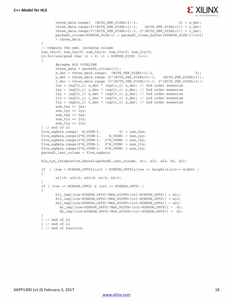
XAPP1300 (v1.0) February 3, 2017 18www.xilinx.com
three_data.range( (BITS_PER_PIXEL+1)-1, 0) = x_der;three_data.range(2*(BITS_PER_PIXEL+1)-1, (BITS_PER_PIXEL+1)) = y_der;three_data.range(3*(BITS_PER_PIXEL+1)-1, 2*(BITS_PER_PIXEL+1)) = t_der;packed3_column[WINDOW_SIZE-1] = packed3_lines_buffer[WINDOW_SIZE-1][col]= three_data;
}// compute the new, incoming columnsum_Ixx=0; sum_Iyy=0; sum_Ixy=0; sum_Itx=0; sum_Ity=0; L3:for(unsigned char ii = 0; ii < WINDOW_SIZE; ii++){
#pragma HLS PIPELINEthree_data = packed3_column[ii];x_der = three_data.range( (BITS_PER_PIXEL+1)-1, 0);y_der = three_data.range (2*(BITS_PER_PIXEL+1)-1, (BITS_PER_PIXEL+1));t_der = three_data.range (3*(BITS_PER_PIXEL+1)-1, 2*(BITS_PER_PIXEL+1));Ixx = (sqflt_t) x_der * (sqflt_t) x_der; // 2nd order momentumIyy = (sqflt_t) y_der * (sqflt_t) y_der; // 2nd order momentumIxy = (sqflt_t) x_der * (sqflt_t) y_der; // 2nd order momentumItx = (sqflt_t) t_der * (sqflt_t) x_der; // 2nd order momentumIty = (sqflt_t) t_der * (sqflt_t) y_der; // 2nd order momentumsum_Ixx += Ixx;sum_Iyy += Iyy;sum_Ixy += Ixy;sum_Itx += Itx;sum_Ity += Ity;
} // end of L3five_sqdata.range( W_VSUM-1, 0) = sum_Ixx; five_sqdata.range(2*W_VSUM-1, W_VSUM) = sum_Iyy;five_sqdata.range(3*W_VSUM-1, 2*W_VSUM) = sum_Ixy;five_sqdata.range(4*W_VSUM-1, 3*W_VSUM) = sum_Itx;five_sqdata.range(5*W_VSUM-1, 4*W_VSUM) = sum_Ity;packed5_last_column = five_sqdata;
hls_tyx_integration_kernel(packed5_last_column, a11, a12, a22, b1, b2);
if ( (row < WINDOW_OFFS)&(col < WINDOW_OFFS)&(row >= height)&(col>= width) ){
a11=0; a12=0; a22=0; b1=0; b2=0;}if ( (row >= WINDOW_OFFS) & (col >= WINDOW_OFFS) ) {
A11_img[(row-WINDOW_OFFS)*MAX_WIDTH+(col-WINDOW_OFFS)] = a11; A12_img[(row-WINDOW_OFFS)*MAX_WIDTH+(col-WINDOW_OFFS)] = a12; A22_img[(row-WINDOW_OFFS)*MAX_WIDTH+(col-WINDOW_OFFS)] = a22;
B1_img[(row-WINDOW_OFFS)*MAX_WIDTH+(col-WINDOW_OFFS)] = b1; B2_img[(row-WINDOW_OFFS)*MAX_WIDTH+(col-WINDOW_OFFS)] = b2;
}} // end of L2} // end of L1} // end of function

C++ Model for HLS
XAPP1300 (v1.0) February 3, 2017 19www.xilinx.com
hls_txy_integration_kernel() Routine C/C++ Code Fragment
void hls_tyx_integration_kernel(p5sqflt_t packed5_last_column,sum_t &a11, sum_t &a12, sum_t &a22, sum_t &b1, sum_t &b2)
{
static p5sqflt_t packed5_window[WINDOW_SIZE];#pragma HLS ARRAY_PARTITION variable=packed5_window complete dim=1
// local accumulatorsstatic sum_t sum_Ixx, sum_Ixy, sum_Iyy, sum_Ity, sum_Itx;
vsum_t sum_xx, sum_xy, sum_yy, sum_tx, sum_ty;p5sqflt_t five_sqdata, packed5_first_column;
//Shift right the sliding window to make room for the new columnpacked5_first_column = packed5_window[0];L0:for(unsigned char jj = 0; jj < WINDOW_SIZE-1; jj++){
packed5_window[jj] = packed5_window[jj+1];}packed5_window[WINDOW_SIZE-1] = packed5_last_column;
//Compute the 2D integration//add incoming right-most column five_sqdata = packed5_window[WINDOW_SIZE-1];sum_xx = five_sqdata.range( W_VSUM-1, 0);sum_yy = five_sqdata.range(2*W_VSUM-1, W_VSUM);sum_xy = five_sqdata.range(3*W_VSUM-1, 2*W_VSUM);sum_tx = five_sqdata.range(4*W_VSUM-1, 3*W_VSUM);sum_ty = five_sqdata.range(5*W_VSUM-1, 4*W_VSUM);sum_Ixx += sum_xx; sum_Ixy += sum_xy;sum_Iyy += sum_yy; sum_Ity += sum_ty;sum_Itx += sum_tx;
//remove older left-most columnfive_sqdata = packed5_first_column;sum_xx = five_sqdata.range( W_VSUM-1, 0);sum_yy = five_sqdata.range(2*W_VSUM-1, W_VSUM);sum_xy = five_sqdata.range(3*W_VSUM-1, 2*W_VSUM);sum_tx = five_sqdata.range(4*W_VSUM-1, 3*W_VSUM);sum_ty = five_sqdata.range(5*W_VSUM-1, 4*W_VSUM);sum_Ixx -= sum_xx; sum_Ixy -= sum_xy;sum_Iyy -= sum_yy; sum_Ity -= sum_ty;sum_Itx -= sum_tx;
a11 = sum_Ixx; a12 = sum_Ixy; a22 = sum_Iyy; b1 = sum_Itx; b2 = sum_Ity;}

C++ Model for HLS
XAPP1300 (v1.0) February 3, 2017 20www.xilinx.com
hls_ComputeVectors() This function computes the vx and vy vector components by solving Equation 6, as shown in Equation 7, via the innermost hls_matrix_inversion() routine, which is the only function using floating point operations in the LK optical flow design.
Note: The 2x2 matrix cannot be inverted if detA is null or if it is below a certain threshold.
Because the elements of the matrix have large values (30 bits in case of an 8-bit input pixel and a 53x53 integration window), the threshold is 1.0 with normalized data generated by ComputeIntegrals(). However, this last routine does not have the normalization per the integration window size. Consequently, to compensate, the actual threshold is 1.0 x WINDOW_SIZE x WINDOW_SIZE.
The final motion vector components are then multiplied by eight and truncated into 16-bit values of which 3 bits are for subpixel accuracy (as SUBPIX_BITS=3 in this design), which means 1/8 of pixel.
Equation 7
The most important C/C++ code fragments for these two routines are listed here:
ComputeVectors() Routine C/C++ Code Fragment
typedef ap_int<2*W_VSUM> sum2_t; // for matrix inversiontypedef ap_int<2*W_VSUM+3> det_t; // for determinant in matrix inversion
float Vx, Vy; signed short int qVx, qVy; A[0][0] = A11_img[(row)*MAX_WIDTH+(col)];//a11A[0][1] = A12_img[(row)*MAX_WIDTH+(col)]; //a12; A[1][0] = A[0][1]; //a21A[1][1] = A22_img[(row)*MAX_WIDTH+(col)]; //a22;B[0] = B1_img[(row)*MAX_WIDTH+(col)]; //b1B[1] = B2_img[(row)*MAX_WIDTH+(col)]; //b2
bool invertible = hls_matrix_inversion(A, B, THRESHOLD, Vx, Vy);cnt = cnt + ((int) invertible); //number of invertible points found
//quantize motion vectorsout_vx[(row)*MAX_WIDTH+(col)] = (signed short int ) (Vx *(1<<SUBPIX_BITS));out_vy[(row)*MAX_WIDTH+(col)] = (signed short int ) (Vy *(1<<SUBPIX_BITS));
vx
vy
A22 A12–
A12– A11
B0
B1
1det A--------------⋅ ⋅=
det A A11 A22 A12– A12⋅ ⋅=

C++ Model for HLS
XAPP1300 (v1.0) February 3, 2017 21www.xilinx.com
hls_matrix_inversion() Routine C/C++ Code Fragment
bool hls_matrix_inversion(sum_t A[2][2], sum_t B[2], int threshold, float &Vx, float &Vy){
bool invertible = 0;sum_t inv_A[2][2], a, b, c, d; det_t det_A, abs_det_A, neg_det_A, zero = 0;float recipr_det_A;
a = A[0][0]; b = A[0][1]; c = A[1][0]; d = A[1][1];
sum2_t a_x_d, b_x_c, mult1, mult2, mult3, mult4;det_t t_Vx, t_Vy;
a_x_d = (sum2_t) a * (sum2_t) d;b_x_c = (sum2_t) b * (sum2_t) c;det_A = a_x_d - b_x_c;neg_det_A = (zero-det_A);abs_det_A = (det_A > zero)? det_A : neg_det_A;recipr_det_A = (1.0f)/det_A;
//compute the inverse of matrix A anywayif (det_A == 0) recipr_det_A = 0;inv_A[0][0] = d;inv_A[0][1] = -b; inv_A[1][0] = -c; inv_A[1][1] = a;
mult1 = (sum2_t) inv_A[0][0] * (sum2_t) B[0];mult2 = (sum2_t) inv_A[0][1] * (sum2_t) B[1];mult3 = (sum2_t) inv_A[1][0] * (sum2_t) B[0];mult4 = (sum2_t) inv_A[1][1] * (sum2_t) B[1];t_Vx = -(mult1 + mult2);t_Vy = -(mult3 + mult4);Vx = t_Vx * recipr_det_A;Vy = t_Vy * recipr_det_A;
if (det_A == 0) { // zero input pixelsinvertible = 0; Vx = 0; Vy = 0;
}else if (abs_det_A < threshold) { // the matrix is not invertible
invertible = 0; Vx = 0; Vy = 0;}else invertible = 1;
return invertible;}
hls_LK() This function implements the same block diagram as shown in Figure 1 and becomes the top-level module in the RTL (Verilog or VHDL) generated by Vivado HLS. The two input images are limited to 16 bits per pixel because of the possibility of using more than 8 bits per pixel in future designs, and because the SDSoC environment needs interfaces to the memory subsystem of the ARM® processor aligned to 8, 16, 32, or 64 bits. All of the data types so far automatically increase the amount of bits depending on the number of bits per input pixel, based on C++ templates in HLS. The output image has samples of 32 bits. Each sample is a packed word of two 16-bit motion vector components (vx and vy). The input and output images are declared to have a FIFO interface via the pragma HLS INTERFACE directive.

C++ Model for HLS
XAPP1300 (v1.0) February 3, 2017 22www.xilinx.com
The ten local 2D arrays are transformed into streams of 10 (HLS_STREAM_DEPTH) registers deep via the pragma HLS STREAM directive. The four inner routines are transformed into concurrent processes via the pragma HLS DATAFLOW directive and each stream is produced and consumed only once. The C/C++ code fragment is shown in Top-level Function hls_LK() Routine to be Synthesized C/C++ Code Fragment.
Top-level Function hls_LK() Routine to be Synthesized C/C++ Code Fragment
const int HLS_STREAM_DEPTH = 10;
int hls_LK(unsigned short int inp1_img[MAX_HEIGHT*MAX_WIDTH], unsigned short int inp2_img[MAX_HEIGHT*MAX_WIDTH], signed short int out_vx[MAX_HEIGHT*MAX_WIDTH], signed short int out_vy[MAX_HEIGHT*MAX_WIDTH], unsigned short int height, unsigned short int width){
#pragma HLS INTERFACE ap_fifo port=inp1_img#pragma HLS INTERFACE ap_fifo port=inp2_img#pragma HLS INTERFACE ap_fifo port=out_Vxy
#pragma HLS DATAFLOW
sum_t A11_img[MAX_HEIGHT*MAX_WIDTH];sum_t A12_img[MAX_HEIGHT*MAX_WIDTH];sum_t A22_img[MAX_HEIGHT*MAX_WIDTH];sum_t B1_img[MAX_HEIGHT*MAX_WIDTH];sum_t B2_img[MAX_HEIGHT*MAX_WIDTH];flt_t Dx1_img[MAX_HEIGHT*MAX_WIDTH]; // horizontal derivativeflt_t Dy1_img[MAX_HEIGHT*MAX_WIDTH]; // vertical derivativeflt_t Dt_img[MAX_HEIGHT*MAX_WIDTH]; // temporal derivativepix_t flt1_img[MAX_HEIGHT*MAX_WIDTH]; // filtered imagespix_t flt2_img[MAX_HEIGHT*MAX_WIDTH];
#pragma HLS STREAM variable=A11_img depth=HLS_STREAM_DEPTH#pragma HLS STREAM variable=A12_img depth=HLS_STREAM_DEPTH#pragma HLS STREAM variable=A22_img depth=HLS_STREAM_DEPTH#pragma HLS STREAM variable=B1_img depth=HLS_STREAM_DEPTH#pragma HLS STREAM variable=B2_img depth=HLS_STREAM_DEPTH#pragma HLS STREAM variable=Dx1_img depth=HLS_STREAM_DEPTH#pragma HLS STREAM variable=Dy1_img depth=HLS_STREAM_DEPTH#pragma HLS STREAM variable=Dt_img depth=HLS_STREAM_DEPTH#pragma HLS STREAM variable=flt1_img depth=HLS_STREAM_DEPTH#pragma HLS STREAM variable=flt2_img depth=HLS_STREAM_DEPTH
// smooth both images with same 2D filter kernelhls_twoIsotropicFilters(inp1_img, inp2_img, flt1_img, flt2_img, height, width);//compute horizontal & vertical derivatives of image 1, plus temporal derivativehls_SpatialTemporalDerivatives(flt1_img, flt2_img, Dx1_img, Dy1_img, Dt_img, height, width);// compute integrals of second order momenta Ixx, Ixy, Iyy, Itx, Ityhls_ComputeIntegrals(Dx1_img, Dy1_img, Dt_img, A11_img, A12_img, A22_img, B1_img, B2_img, height, width);// compute vectorsint cnt = hls_ComputeVectors(A11_img, A12_img, A22_img, B1_img, B2_img, out_vx, out_vy, height, width);
return cnt;}
HLS Design Performance
XAPP1300 (v1.0) February 3, 2017 23www.xilinx.com
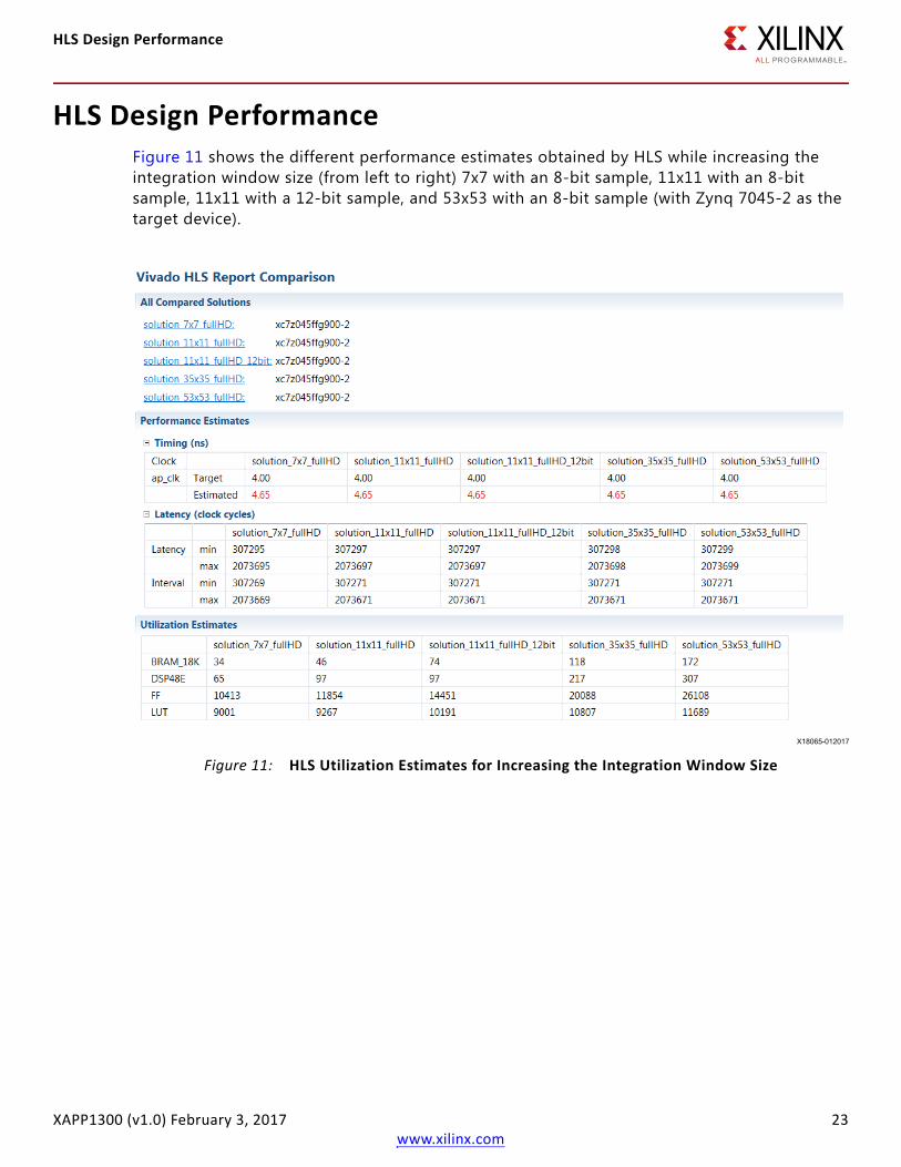
HLS Design PerformanceFigure 11 shows the different performance estimates obtained by HLS while increasing the integration window size (from left to right) 7x7 with an 8-bit sample, 11x11 with an 8-bit sample, 11x11 with a 12-bit sample, and 53x53 with an 8-bit sample (with Zynq 7045-2 as the target device).
X-Ref Target - Figure 11
Figure 11: HLS Utilization Estimates for Increasing the Integration Window Size
X18065-012017

HLS Design Performance
XAPP1300 (v1.0) February 3, 2017 24www.xilinx.com
The implementation results after place and route (PAR) are listed in Table 1 and Table 2. Table 1 summarizes the performance in terms of FPGA resources and achieved frame rate. Specifically for the 53x53 integration window size, the results are 172 BRAM18K, 307 DSP48, 9881 FF, and 7001 LUTs with a frame rate of about 121 Hz (given by the effective clock period of 3.976 ns and the latency of 2073697 clock cycles measured during C/RTL cosimulation). In Table 1, the shaded row is for an input image with 12-bit pixels. The other rows are for 8-bit input samples.
Different applications might need different integration window sizes. In this section, the 53x53 integration window size is used as an example because it represents the most challenging design. Table 2 shows the possible trade-offs between using DSP48 resources or using FF/LUT resources for implementing the multiplications within the ComputeIntegrals() routine. By adding the HLS RESOURCE directive to none or to all of the five variables Ixx, Iyy, Ixy, Itx, Ity in the hls_ComputeIntegrals() Routine C/C++ Code Fragment, the number of DSP48 resources can be decreased from 307 (if five multiplications are done on DSP48 slices) to 197 (if four multiplications are done on DSP48 slices) or to 38 (if no multiplications are done on DSP48). Consequently, the number of FF/LUT resources increases from 9881/7001 to 16044/17779 or to 22160/32476, respectively. Which of these results is the best one is an architectural choice that depends on other design factors at the system level (for example, the number of resources available on the same target device to run other functionalities, or the required frame rate of work), similar to the integration window size. The C/C++ code fragment in HLS Resource Directive Assigns Variables to LUT-based Multipliers shows how the HLS RESOURCE directive has been applied to make all five multiplications into LUT-based operators.
Table 1: HLS Implementation Results (After Place and Route) for Increasing Integration Window Size
Summary Latency (cycles)
CP(ns)
Clock Frequency
(MHz)
Frame Rate (Hz)
BRAM18K DSP48E FF LUT
1920x1080 resolution 08-bit, 7x7 window, Z-7045 2073697 3.65 274.0 132.1 34 63 8076 4898
1920x1080 resolution 08-bit, 11x11 window, Z-7045 2073697 3.48 287.4 138.6 46 97 8574 4948
1920x1080 resolution 12-bit, 11x11 window, Z-7045 2073697 3.561 280.8 135.4 74 97 10147 5832
1920x1080 resolution 08-bit, 35x35 window, Z-7045 2073697 3.909 255.8 123.4 118 217 9490 6372
1920x1080 resolution 08-bit, 53x53 window, Z-7045 2073697 3.976 251.5 121.3 172 307 9881 7001

HLS Design Performance
XAPP1300 (v1.0) February 3, 2017 25www.xilinx.com
In the last two rows of Table 2, instead of applying the HLS RESOURCE directive to any of the five variables, the overall number of multiplication operations within ComputeIntegrals() is limited to 100 or to 150. This reduces the number of DSP48 resources from 307 to 137 or 187 while FF/LUT resource numbers are 13440/10501 (#pragma HLS ALLOCATION instances=mul limit=100 operation) or 14530/10833 (#pragma HLS ALLOCATION instances=mul limit=150 operation). The major effect of this optimization technique is not only to reduce the DSP48 resources but also to decrease the achievable throughput, which lowers the effective frame rate to 41 Hz or 61 Hz, respectively. This must be a system-level design decision because many image processing applications (typically automotive) with optical flow do not need to operate at more than 15/30 Hz frame rate.
Table 2 highlights a major advantage of Vivado HLS design flow, by adding or removing some directives, different architectural choices can be analyzed and selected based on which one is most suitable to the design requirements for resources and frame rate.
HLS Resource Directive Assigns Variables to LUT-based Multipliers
sqflt_t Ixx, Iyy, Ixy, Itx, Ity;#pragma HLS RESOURCE variable=Ixx core=Mul_LUT #pragma HLS RESOURCE variable=Iyy core=Mul_LUT #pragma HLS RESOURCE variable=Ixy core=Mul_LUT #pragma HLS RESOURCE variable=Itx core=Mul_LUT #pragma HLS RESOURCE variable=Ity core=Mul_LUT
Table 3 and Table 4 show how resources are distributed among the four subroutines called by the top level of the design. The ComputeIntegrals() routine is responsible for most of the BRAM18K, DSP48, and FF utilization. In Table 3, the target device is the Zynq 7045-2 with all multiplications implemented on DSP48 slices and a frame rate of 121 Hz. In Table 4, the target device is the Zynq 7020-1 with the maximum amount of multiplications limited to 150 and a frame rate of 41 Hz.
Table 2: Trade-off Between DSP48 and FF/LUT to Implement Multipliers
1920x1080 Resolution 08-bit,53x53 Window, Z-7045
Latency (cycles)
CP(ns)
Clock Frequency
(MHz)
Frame Rate (Hz)
BRAM18K DSP48E FF LUT
ComputeIntegrals: 5 of 5 9x9 MULS into DSP48 2073697 3.976 251.5 121.3 172 307 9881 7001
ComputeIntegrals: 1of 5 9x9 MULS into FF and LUT 2073697 4.084 244.9 118.1 172 197 16044 17779
ComputeIntegrals: 5 of 5 9x9 MULS into FF and LUT 2073697 4.027 248.3 119.7 172 38 22160 32476
ComputeIntegrals: limiting to 100 all MUL (done in DSP48) 6220818 3.849 259.8 41.8 172 137 13440 10501
ComputeIntegrals: limiting to 150 all MUL (done in DSP48) 4147219 3.91 255.8 61.7 172 187 14530 10833

HLS Design Performance
XAPP1300 (v1.0) February 3, 2017 26www.xilinx.com
Table 3: Detailed View of Resources Utilization on the Zynq 7045-2 Target Device
1920x1080 Resolution 8-bit, PAR Implementation
Function Latency (cycles)
CP(ns)
Clock Frequency
(MHz)
Frame Rate (Hz)
BRAM18K DSP48E FF LUT
TwoIsotropicFilters 8 1 665 1022
SpatialTemporalDerivatives 8 3 316 356
ComputeIntegrals: 5 of 5 9x9 MULS into DSP48 156 266 6804 1881
ComputeVectors 0 37 2060 3436
LK 53x53 integration window 2073697 3.976 251.5 121.3
Total 172 307 9881 7001
Z-7045 available resources 1090 900 437200 218600
Percentage (%) 15.78 34.11 2 3
Table 4: Detailed View of Resources Utilization on the Zynq 7020-1 Target Device
1920x1080 Resolution 8-bit, PAR Implementation
Function Latency (Cycles)
CP(ns)
Clock Frequency
(MHz)
Frame Rate (Hz)
BRAM18K DSP48E FF LUT
TwoIsotropicFilters 8 1 1351 1022
SpatialTemporalDerivatives 8 3 627 354
ComputeIntegrals: limiting to 150 all MUL (done in DSP48) 156 150 13305 6057
ComputeVectors 0 33 3583 3350
LK 53x53 integration window 4147222 5.859 170.7.5 41.2
Total 172 187 18930 11083
Z-7020 available resources 280 220 106400 53200
Percentage (%) 61.43 85.00 17.79 20.83

SDSoC Demonstration on ZC706 Board
XAPP1300 (v1.0) February 3, 2017 27www.xilinx.com
SDSoC Demonstration on ZC706 BoardThe easiest way to validate the HLS design of the LK optical flow is by implementing it in one of the Zynq-7000 AP SoC boards (either the ZC702 or the ZC706) where the input signal is from a digital video sequence file and the output is written to a file. In this way, the focus can be on the LK optical flow core itself, which eliminates designing a more complicated system with real-time high-definition multimedia interface (HDMI™) video signals and related frame buffers. With the SDSoC development environment, designing an I/O demonstration file on a Zynq-7000 AP SoC board requires only a few hours of work. The code fragment in Top-level Function hls_LK() Routine to be Synthesized C/C++ Code Fragment is suitable to the SDSoC environment. In this code fragment, the I/O parameters of the function prototype are true ANSI-C data types and are aligned to 8, 16, or 32-bits in the memory space of the ARM CPU (see SDSoC Environment User Guide [Ref 4]).
The SDSoC directives applied to the top-level function prototype (in the header file LK_defines.h) are shown in SDSoC Directives to the Top-level Function Prototype.
SDSoC Directives to the Top-level Function Prototype
#ifdef __SDSCC__#pragma SDS data access_pattern(inp1_img:SEQUENTIAL)#pragma SDS data access_pattern(inp2_img:SEQUENTIAL)#pragma SDS data access_pattern( vx_img:SEQUENTIAL)#pragma SDS data access_pattern( vy_img:SEQUENTIAL)#pragma SDS data copy(inp1_img[0:hls_IMGSZ])#pragma SDS data copy(inp2_img[0:hls_IMGSZ])#pragma SDS data copy( vx_img[0:hls_IMGSZ])#pragma SDS data copy( vy_img[0:hls_IMGSZ])#pragma SDS data sys_port(inp1_img:ACP,inp2_img:ACP,vx_img:ACP,vy_img:ACP)#endifint hls_LK(unsigned short int *inp1_img, unsigned short int *inp2_img,
signed short int *vx_img, signed short int *vy_img, unsigned short int height, unsigned short int width);
• The SDS data access_pattern directive specifies that all I/O arrays will have a sequential access pattern and, consequently, the SDSoC environment will implement a FIFO interface.
• The SDS data copy directive specifies the overall payload size of the DMA communication transfers.
• The SDS data sys_port directive connects the interfaces of the FPGA hardware accelerator to the accelerator coherency post (ACP) of the ARM memory subsystem.
Note: The __SDSCC__ is a prebuilt C pre-processor macro recognized only by SDSoC compilers and ignored by other compilers (for example, Vivado HLS compiler).
The most important C/C++ code fragments of the main() routine composing the self-checking functional test bench for either HLS or the SDSoC environment are listed in SDSoC Functional Test Bench C/C++ Code Fragment. Using the predefined macros __SYNTHESIS__ and __SDSCC__ for HLS and the SDSoC environment, respectively, makes it easy to write software that can be seen only by one or the other compiler, which reduces development time.

SDSoC Demonstration on ZC706 Board
XAPP1300 (v1.0) February 3, 2017 28www.xilinx.com
SDSoC Functional Test Bench C/C++ Code Fragment
int main(int argc, char** argv){
unsigned short x, y, width, height;int check_results, ret_res=0, ref_pt, inv_points;unsigned short *inp1_img, *inp2_img; signed short *vx_ref, *vy_ref, *vx_img, *vy_img; // memory allocationvx_ref =( signed short *) malloc(MAX_HEIGHT*MAX_WIDTH*sizeof(signed short));vy_ref =( signed short *) malloc(MAX_HEIGHT*MAX_WIDTH*sizeof(signed short));inp1_img=(unsigned short*)sds_alloc(MAX_HEIGHT*MAX_WIDTH*sizeof(unsigned short));inp2_img=(unsigned short*)sds_alloc(MAX_HEIGHT*MAX_WIDTH*sizeof(unsigned short));vx_img =( signed short*)sds_alloc(MAX_HEIGHT*MAX_WIDTH*sizeof( signed short));vy_img =( signed short*)sds_alloc(MAX_HEIGHT*MAX_WIDTH*sizeof( signed short));
printf("REF design\n");for (int i = 0; i < NUM_TESTS; i++) {sw_sds_clk_start() ref_pt = ref_LK(inp1_img, inp2_img, vx_ref, vy_ref, MAX_HEIGHT, MAX_WIDTH); sw_sds_clk_stop()}printf("num of invertible pt = %d, which represents %2.2f%%\n", ref_pt, (ref_pt*100.0)/(height*width));
printf("HLS DUT\n");for (int i = 0; i < NUM_TESTS; i++) { hw_sds_clk_start() inv_points = hls_LK(inp1_img, inp2_img, vx_img, vy_img, MAX_HEIGHT, MAX_WIDTH); hw_sds_clk_stop() }printf("numb of invertible pt = %d, which represents %2.2f%%\n", inv_points, (inv_points*100.0)/(height*width));sds_print_results()
// self checking test benchprintf("Checking results: REF vs. HLS\n");double diff1, abs_diff1, diff2, abs_diff; check_results = 0;L1:for (y=(WINDOW_OFFS+2*FILTER_OFFS); y < height-(WINDOW_OFFS+2*FILTER_OFFS); y++){L2:for (x=(WINDOW_OFFS+2*FILTER_OFFS); x < width -(WINDOW_OFFS+2*FILTER_OFFS); x++{ int vect1x, vect2x, vect1y, vect2y; vect1x = vx_img[y*MAX_WIDTH + x]; vect2x = vx_ref[y*MAX_WIDTH + x]; vect1y = vy_img[y*MAX_WIDTH + x]; vect2y = vy_ref[y*MAX_WIDTH + x]; diff1 = vect2x - vect1x; diff2 = vect2y - vect1y; abs_diff1 = ABS(diff1); abs_diff2 = ABS(diff2); if (abs_diff1 > 1) { printf("Vx: expected %20.10f got %20.10f\n", (float) vect2x, (float) vect1x);check_results++;
} if (abs_diff2 > 1) { printf("Vy: expected %20.10f got %20.10f\n", (float) vect2y, (float) vect1y);check_results++;
}} // end of L1} // end of L2
printf("Test done\n");

SDSoC Demonstration on ZC706 Board
XAPP1300 (v1.0) February 3, 2017 29www.xilinx.com
if (check_results > MAX_NUM_OF_WRONG_VECTORS) { printf("TEST FAILED!: error = %d\n", check_results); ret_res = 1; }else { printf("TEST SUCCESSFUL!\n"); ret_res = 0; }
// free memoryfree(vx_ref); free(vy_ref); sds_free(inp1_img); sds_free(inp2_img); sds_free(vx_img); sds_free(vy_img);
return ret_res;
}
Specifically, sds_alloc is the SDSoC memory allocator that generates dynamic memory contiguously paged on both virtual and physical memory spaces of Linux OS, and consequently requires DMA_SIMPLE as a data mover to connect the accelerator ports with the ARM memory subsystem ports. The DMA_SIMPLE uses fewer CPU clock cycles for setup and fewer FPGA resources than the more powerful scatter gather DMA (DMA_SG). The DMA_SG can map contiguously paged virtual memory in non-contiguously paged physical memory without limitations on the payload size, but the DMA_SIMPLE has a payload size limit of 8 MB. For any data movement larger than 8 MB, the DMA_SG is automatically instantiated by the SDSoC environment.
To smooth D-cache misses, the reference and the design under test (DUT) functions are launched NUM_TESTS number of times, and consequently emulate a realistic scenario where a long video sequence is processed.
The sw_sds_clock_start(), sw_sds_clock_stop(), hw_sds_clock_start(), and hw_sds_clock_stop() are SDSoC environment predefined macros that call the 64-bit ARM performance counters and consequently measure the execution time directly in CPU clock cycles at run time. They are ignored during purely HLS design flow.
In a bottom-up approach from HLS to the SDSoC environment, it is good practice to run HLS C-to-RTL cosimulation to verify that the RTL generated by HLS is working correctly, especially in standalone mode. Also, running HLS implementation with PAR can reveal any possible problems meeting timing constraints for the standalone core before integrating it into a larger design with the SDSoC environment. With a 35x35 integration window size and a limit of 150 multiplication operations in the ComputeIntegrals() routine (which can fit in either ZC702 or ZC706 boards). Figure 12 and Figure 13 illustrate the HLS cosimulation and implementation reports, respectively. Figure 14 shows the data motion network report of the embedded system automatically generated by the SDSoC environment. Figure 15 shows the application output during run time execution on the ZC706 board. The hardware accelerator running at 150 MHz is 68 times faster than the purely software execution on the ARM CPU running at 800 MHz.

SDSoC Demonstration on ZC706 Board
XAPP1300 (v1.0) February 3, 2017 30www.xilinx.com
X-Ref Target - Figure 12
Figure 12: HLS Cosimulation Report for 35x35 IntegrationWindow Size with 150 Multiplications Limit
X-Ref Target - Figure 13
Figure 13: HLS Implementation Report for 35x35 IntegrationWindow Size with 150 Multiplications Limit
X18066-012017
X18067-012017

SDSoC Demonstration on ZC706 Board
XAPP1300 (v1.0) February 3, 2017 31www.xilinx.com
X-Ref Target - Figure 14
Figure 14: Data Motion Network Report of the Embedded System Generated by SDSoC
X18068-012017

SDSoC Demonstration on ZC706 Board
XAPP1300 (v1.0) February 3, 2017 32www.xilinx.com
X-Ref Target - Figure 15
Figure 15: Run Time Execution on ZC706 Board
X18069-012017

More on HLS Optimization Techniques
XAPP1300 (v1.0) February 3, 2017 33www.xilinx.com
More on HLS Optimization TechniquesThis optical flow design applies sophisticated HLS optimization techniques to achieve the best trade-off between a high frame rate and a small number of FPGA resources. These are opposite performance requirements because the higher the frame rate, the larger the necessary parallelism of operations to sustain the data throughput. Assuming this optical flow core is just one in an image processing pipeline (for example, to track objects), it is very important to save block RAMs, LUTs, DSP48s, and FFs because image processing routines can consume large numbers of these resources.
Saving BRAM18KPacking two pixels with the same coordinates of the two input images into a larger word (see dual_pix_t data type of Packing Two Pixels Into a Larger Word With HLS C++ Range Operator) is the key to saving BRAM18K in the hls_twoIsotropicFilter() routine. Assuming to have used two separate sliding windows and line buffers as shown in the code fragment in Version of hls_twoIsotropicFilters Not Optimized to Save BRAM18K (this code can be enabled by defining the macro ISOTROPIC_NOT_OPTIMIZED), the Vivado HLS compiler is not able to generate fewer block RAMS when the input pixel is larger than 8 bits (for example, 12 bits). The HLS synthesis reports shown in Figure 16 demonstrate that if the block RAM amount is the same for 8-bit samples in the not optimized (Version of hls_twoIsotropicFilters Not Optimized to Save BRAM18K) and optimized (Packing Two Pixels Into a Larger Word With HLS C++ Range Operator) versions of hls_twoIsotropicFilter(), there is an advantage with fewer block RAMs for 12-bit samples.
Version of hls_twoIsotropicFilters Not Optimized to Save BRAM18K
#ifdef ISOTROPIC_NOT_OPTIMIZEDvoid hls_twoIsotropicFilters(. . . ){pix_t filt_out1, filt_out2, pix1, pix2;pix_t pixel1[FILTER_SIZE], pixel2[FILTER_SIZE];pix_t window1[FILTER_SIZE*FILTER_SIZE];#pragma HLS ARRAY_PARTITION variable=window1 complete dim=0pix_t window2[FILTER_SIZE*FILTER_SIZE];#pragma HLS ARRAY_PARTITION variable=window2 complete dim=0static pix_t lpf1_line_buffer[FILTER_SIZE][MAX_WIDTH];#pragma HLS ARRAY_PARTITION variable=lpf1_line_buffer complete dim=1static pix_t lpf2_line_buffer[FILTER_SIZE][MAX_WIDTH];#pragma HLS ARRAY_PARTITION variable=lpf2_line_buffer complete dim=1
// effective filteringL1: for(row = 0; row < height+FILTER_OFFS; row++)
{#pragma HLS LOOP_TRIPCOUNT max=480L2: for(col = 0; col < width+FILTER_OFFS; col++)
{#pragma HLS PIPELINE II=1#pragma HLS LOOP_TRIPCOUNT max=640
// Line Buffer fillif(col < width)

More on HLS Optimization Techniques
XAPP1300 (v1.0) February 3, 2017 34www.xilinx.com
for(unsigned char ii = 0; ii < FILTER_SIZE-1; ii++) {pixel1[ii] = lpf1_line_buffer[ii][col]
= lpf1_line_buffer[ii+1][col];pixel2[ii] = lpf2_line_buffer[ii][col]
= lpf2_line_buffer[ii+1][col];}
//There is an offset to accomodate the active pixel regionif((col < width) && (row < height)){pix1 = inp1_img[row*MAX_WIDTH+col];pix2 = inp2_img[row*MAX_WIDTH+col];pixel1[FILTER_SIZE-1] = lpf1_line_buffer[FILTER_SIZE-1][col] = pix1;pixel2[FILTER_SIZE-1] = lpf2_line_buffer[FILTER_SIZE-1][col] = pix2;
}. . .
These optimization techniques are used in the hls_SpatialTemporal-Derivatives() and ComputeIntegrals() in the 2D Convolution of hls_derivatives_kernel() and hls_ComputeIntegrals() Routine C/C++ Code Fragment routines. In this case, three 9-bit data are packed into a 27-bit larger word for 8-bit samples (or three 13-bit data are packed into a 39-bit larger word for 12 bits per pixel).
X-Ref Target - Figure 16
Figure 16: Synthesis Estimated Resources Comparison between Optimizedand Not Optimized Version of hls_twoIsotropicFilters
X18070-012017

More on HLS Optimization Techniques
XAPP1300 (v1.0) February 3, 2017 35www.xilinx.com
Saving Flip-Flops and LUTsIn the unoptimized version of ComputeIntegrals(), the entire sliding window is passed to the innermost hls_tyx_integration_kernel(), which computes five times NxN accumulations, as shown in hls_txy_integration_kernel() Not Optimized Routine C/C++ Code Fragment (this code can be enabled by defining the macro INTEGRALS_NOT_OPTIMIZED).
Note: The multiplications to compute the five parameters Ixx, Ixy, Iyy, Itx, and Ity are completed outside of the function to avoid redundant operations, although the accumulations are still too many in comparison with the optimized version in hls_ComputeIntegrals() Routine C/C++ Code Fragment.
The HLS estimation comparison of two solutions for the 53x53 integration window size is shown in Figure 17.
hls_txy_integration_kernel() Not Optimized Routine C/C++ Code Fragment
#ifdef INTEGRALS_NOT_OPTIMIZEDvoid hls_tyx_integration_kernel(p5sqflt_t packed_window[WINDOW_SIZE*WINDOW_SIZE],
sum_t &a11, sum_t &a12, sum_t &a22, sum_t &b1, sum_t &b2) {
// local accumulatorssum_t sum_xx = (sum_t) 0; sum_t sum_xy = (sum_t) 0;sum_t sum_yy = (sum_t) 0; sum_t sum_ty = (sum_t) 0;sum_t sum_tx = (sum_t) 0;
sqflt_t mult_xx, mult_xy, mult_yy, mult_tx, mult_ty;p5sqflt_t five_sqdata;
unsigned short int i;//Compute the 2D integrationL1:for (i = 0; i < WINDOW_SIZE*WINDOW_SIZE; i++){ five_sqdata = packed_window[i]; mult_xx = five_sqdata( 2*(BITS_PER_PIXEL+1)-1, 0); mult_yy = five_sqdata( 4*(BITS_PER_PIXEL+1)-1, 2*(BITS_PER_PIXEL+1)); mult_xy = five_sqdata( 6*(BITS_PER_PIXEL+1)-1, 4*(BITS_PER_PIXEL+1)); mult_tx = five_sqdata( 8*(BITS_PER_PIXEL+1)-1, 6*(BITS_PER_PIXEL+1)); mult_ty = five_sqdata(10*(BITS_PER_PIXEL+1)-1, 8*(BITS_PER_PIXEL+1)); sum_xx += mult_xx; sum_xy += mult_xy; sum_yy += mult_yy; sum_ty += mult_ty; sum_tx += mult_tx;}
a11 = sum_xx; a12 = sum_xy; a22 = sum_yy; b1 = sum_tx; b2 = sum_ty;}

More on HLS Optimization Techniques
XAPP1300 (v1.0) February 3, 2017 36www.xilinx.com
Saving DSP48 Slices at Expense of Block RAMAs shown in Table 1, page 24, the number of DSP48 slices increases linearly with the side width (N) of the integration window, which causes the complexity of the hls_ComputeIntegrals() subroutine to be O(N) from a computer science formal point of view. As the sliding window moves one column from the left to the right, the entire incoming rightmost column is added and the old leftmost column is subtracted, as shown in Figure 10. A better way to dramatically optimize the subroutine is by maintaining a column sum for the whole image width and updating the column sum upon the window move by adding the bottom-right sample (the current sample in the streaming order), and subtracting the top-right sample only. In this way, the complexity of the algorithm is independent of the window side N (which is also the column length). This technique is similar to the summed area table method [Ref 10] that is used in image processing. This technique allows a constant calculation time that is independent of the size of the rectangular area compute, thus achieving an O(1) complexity.
The code shown in hls_ComputeIntegrals() Most Optimized Routine C/C++ Code Fragment (this code can be enabled by defining the macro OPTIMIZED_TO_SAVE_DSP48) implements this technique. The comments in the code refer to Figure 18, where only one of the five parameters is illustrated for conciseness and clarity (for example, Ixx).
X-Ref Target - Figure 17
Figure 17: Synthesis Estimated Resources Comparison of Optimized and Not Optimized Version of hls_txy_integration_kernel() for a 53x53 Integration Window Size
X18071-012017

More on HLS Optimization Techniques
XAPP1300 (v1.0) February 3, 2017 37www.xilinx.com
hls_ComputeIntegrals() Most Optimized Routine C/C++ Code Fragment
#ifdef OPTIMIZED_TO_SAVE_DSP48
void hls_ComputeIntegrals(flt_t Ix_img[MAX_HEIGHT*MAX_WIDTH], flt_t Iy_img[MAX_HEIGHT*MAX_WIDTH], flt_t It_img[MAX_HEIGHT*MAX_WIDTH], sum_t A11_img[MAX_HEIGHT*MAX_WIDTH], sum_t A12_img[MAX_HEIGHT*MAX_WIDTH], sum_t A22_img[MAX_HEIGHT*MAX_WIDTH],
sum_t B1_img[MAX_HEIGHT*MAX_WIDTH], sum_t B2_img[MAX_HEIGHT*MAX_WIDTH], unsigned short int height, unsigned short int width) {
unsigned short int row, col; sum_t a11, a12, a22, b1, b2; flt_t x_der, y_der, t_der;p3dtyx_t three_data, packed3_column[WINDOW_SIZE+1];static p3dtyx_t packed3_lines_buffer[WINDOW_SIZE+1][MAX_WIDTH];#pragma HLS ARRAY_PARTITION variable=packed3_lines_buffer complete dim=1sqflt_t top_Ixx, top_Iyy, top_Ixy, top_Itx, top_Ity;sqflt_t bot_Ixx, bot_Iyy, bot_Ixy, bot_Itx, bot_Ity;
// sliding window sums. Gray color cell in Figure 18.staticint sum_Ixx, sum_Ixy, sum_Iyy, sum_Itx, sum_Ity;
// column sums for the entire image width. Yellow color cells in Figure 18static int csIxix[MAX_WIDTH], csIxiy[MAX_WIDTH], csIyiy[MAX_WIDTH], csDix[MAX_WIDTH];static int csDiy[MAX_WIDTH], cbIxix[MAX_WIDTH], cbIxiy[MAX_WIDTH], cbIyiy[MAX_WIDTH];static int cbDix[MAX_WIDTH], cbDiy[MAX_WIDTH];#pragma HLS RESOURCE variable=csIxix core=RAM_2P_BRAM#pragma HLS RESOURCE variable=csIxiy core=RAM_2P_BRAM#pragma HLS RESOURCE variable=csIyiy core=RAM_2P_BRAM#pragma HLS RESOURCE variable=csDix core=RAM_2P_BRAM#pragma HLS RESOURCE variable=csDiy core=RAM_2P_BRAM#pragma HLS RESOURCE variable=cbIxix core=RAM_2P_BRAM#pragma HLS RESOURCE variable=cbIxiy core=RAM_2P_BRAM#pragma HLS RESOURCE variable=cbIyiy core=RAM_2P_BRAM#pragma HLS RESOURCE variable=cbDix core=RAM_2P_BRAM#pragma HLS RESOURCE variable=cbDiy core=RAM_2P_BRAM#pragma HLS DEPENDENCE variable=csIxix inter WAR false#pragma HLS DEPENDENCE variable=cbIxix inter WAR false#pragma HLS DEPENDENCE variable=cbIxiy inter WAR false#pragma HLS DEPENDENCE variable=cbIyiy inter WAR false#pragma HLS DEPENDENCE variable=cbDix inter WAR false#pragma HLS DEPENDENCE variable=cbDiy inter WAR false#pragma HLS DEPENDENCE variable=csIxiy inter WAR false#pragma HLS DEPENDENCE variable=csIyiy inter WAR false#pragma HLS DEPENDENCE variable=csDix inter WAR false#pragma HLS DEPENDENCE variable=csDiy inter WAR false
X-Ref Target - Figure 18
Figure 18: Optimization of ComputeIntegrals to Reduce the Number of DSP48 Slices
X18670-012017

More on HLS Optimization Techniques
XAPP1300 (v1.0) February 3, 2017 38www.xilinx.com
int csIxixR, csIxiyR, csIyiyR, csDixR, csDiyR; // Blue color cell in Figure 18
// the left and right indices onto the column sumsint zIdx = -WINDOW_SIZE; int nIdx = zIdx + WINDOW_SIZE;
L1: for (row = 0; row < height + WINDOW_OFFS; row++) { #pragma HLS LOOP_TRIPCOUNT min=hls_MIN_H max=hls_MAX_HL2: for (col = 0; col < width + WINDOW_OFFS; col++){ #pragma HLS LOOP_TRIPCOUNT min=hls_MIN_W max=hls_MAX_W #pragma HLS PIPELINE
// line-buffer fillif (col < width)for (unsigned char ii = 0; ii < WINDOW_SIZE; ii++) { packed3_column[ii] = packed3_lines_buffer[ii][col] = packed3_lines_buffer[ii + 1][col]; }
if ((col < width) & (row < height)) {x_der = Ix_img[row * MAX_WIDTH + col]; y_der = Iy_img[row * MAX_WIDTH + col]; t_der = It_img[row * MAX_WIDTH + col];
// pack data for the line-bufferthree_data( (BITS_PER_PIXEL + 1) - 1, 0) = x_der;three_data(2 * (BITS_PER_PIXEL + 1) - 1, (BITS_PER_PIXEL + 1)) = y_der;three_data(3 * (BITS_PER_PIXEL + 1) - 1, 2*(BITS_PER_PIXEL + 1)) = t_der;packed3_column[WINDOW_SIZE] = packed3_lines_buffer[WINDOW_SIZE][col] = three_data;// line-buffer done
// the leftSumsint csIxixL = 0, csIxiyL = 0, csIyiyL = 0, csDixL = 0, csDiyL = 0;if (zIdx >= 0){csIxixL = csIxix[zIdx]; csIxiyL = csIxiy[zIdx]; csIyiyL = csIyiy[zIdx];csDixL = csDix[zIdx]; csDiyL = csDiy[zIdx];
}
// incoming column: data on the topthree_data = packed3_column[0];x_der = three_data((BITS_PER_PIXEL + 1) - 1, 0);y_der = three_data(2 * (BITS_PER_PIXEL + 1) - 1, (BITS_PER_PIXEL + 1));t_der = three_data(3 * (BITS_PER_PIXEL + 1) - 1, 2 * (BITS_PER_PIXEL + 1));top_Ixx = (sqflt_t) x_der * (sqflt_t) x_der; top_Iyy = (sqflt_t) y_der * (sqflt_t) y_der;top_Ixy = (sqflt_t) x_der * (sqflt_t) y_der; top_Itx = (sqflt_t) t_der * (sqflt_t) x_der;top_Ity = (sqflt_t) t_der * (sqflt_t) y_der;
// incoming column: data on the bottomthree_data = packed3_column[WINDOW_SIZE];x_der = three_data((BITS_PER_PIXEL + 1) - 1, 0);y_der = three_data(2 * (BITS_PER_PIXEL + 1) - 1, (BITS_PER_PIXEL + 1));t_der = three_data(3 * (BITS_PER_PIXEL + 1) - 1, 2*(BITS_PER_PIXEL + 1));bot_Ixx = (sqflt_t) x_der * (sqflt_t) x_der; bot_Iyy = (sqflt_t) y_der * (sqflt_t) y_der;bot_Ixy = (sqflt_t) x_der * (sqflt_t) y_der; bot_Itx = (sqflt_t) t_der * (sqflt_t) x_der;bot_Ity = (sqflt_t) t_der * (sqflt_t) y_der;
// compute rightSums incrementallycsIxixR=cbIxix[nIdx] + bot_Ixx - top_Ixx; csIxiyR=cbIxiy[nIdx] + bot_Ixy - top_Ixy; csIyiyR=cbIyiy[nIdx] + bot_Iyy - top_Iyy;csDixR = cbDix[nIdx] + bot_Itx - top_Itx; csDiyR= cbDiy[nIdx] + bot_Ity - top_Ity;
// sums += (rightSums - leftLums)sum_Ixx += (csIxixR - csIxixL); sum_Ixy += (csIxiyR - csIxiyL); sum_Iyy += (csIyiyR - csIyiyL);sum_Itx += (csDixR - csDixL); sum_Ity += (csDiyR - csDiyL);
// outputsa11 = sum_Ixx; a12 = sum_Ixy; a22 = sum_Iyy; b1 = sum_Itx; b2 = sum_Ity;
// update new rightSums: Blue cell in State+1 goes to Yellow cell in State+2 of Figure 18cbIxix[nIdx] = csIxixR; cbIxiy[nIdx] = csIxiyR;

More on HLS Optimization Techniques
XAPP1300 (v1.0) February 3, 2017 39www.xilinx.com
cbIyiy[nIdx] = csIyiyR; cbDix[nIdx] = csDixR; cbDiy[nIdx] = csDiyR;csIxix[nIdx] = csIxixR; csIxiy[nIdx] = csIxiyR;csIyiy[nIdx] = csIyiyR; csDix[nIdx] = csDixR; csDiy[nIdx] = csDiyR;
// update indexzIdx++; if (zIdx == width) zIdx = 0; nIdx++; if (nIdx == width) nIdx = 0;
} //end of if ((col < width) & (row < height))
if ((row < WINDOW_OFFS) & (col < WINDOW_OFFS) & (row >= height) & (col >= width)) { a11 = 0; a12 = 0; a22 = 0; b1 = 0; b2 = 0; }if ((row >= WINDOW_OFFS) & (col >= WINDOW_OFFS)) { //output data are not normalized (so that thresholding will be dependent on window size) A11_img[(row - WINDOW_OFFS) * MAX_WIDTH + (col - WINDOW_OFFS)] = a11; A12_img[(row - WINDOW_OFFS) * MAX_WIDTH + (col - WINDOW_OFFS)] = a12; A22_img[(row - WINDOW_OFFS) * MAX_WIDTH + (col - WINDOW_OFFS)] = a22; B1_img[(row - WINDOW_OFFS) * MAX_WIDTH + (col - WINDOW_OFFS)] = b1; B2_img[(row - WINDOW_OFFS) * MAX_WIDTH + (col - WINDOW_OFFS)] = b2;}} // end of L2} // end of L1}
The variables csIxix, csIxiy, csIyiy, csDix, and csDiy model the column sums for the entire image width. These variables are assigned to a dual-port RAM in the block RAM elements with the #pragma HLS RESOURCE variable=… core=RAM_2P_BRAM directive. All block RAM elements are configured with a write-after-read policy that is set with the #pragma HLS DEPENDENCE variable=… inter WAR false directive. This policy relaxes possible dependencies that could impact the HLS scheduling of read/write operations, especially during loop pipelining. Nevertheless, this is not enough for HLS to achieve the II = 1 in the internal loop L2 to sustain the correct data rate. In fact, the effective II value is 2. Consequently, the variables cbIxix, cbIxiy, cbIyiy, cbDix, and cbDiy are added to create more bandwidth and finally achieve II = 1, even if the price is more block RAM elements.
The left-side of Figure 19 shows the comparison of HLS reports for three possible solutions for a 53x53 integration window size. In Figure 19, solution0_ON represents the version of ComputeIntegrals with O(N) complexity using 172 block RAMs, solution0_O1_1mem represents the most optimized routine with O(1) complexity achieving II = 2 using 195 block RAMs, and solution1_O1 represents the most optimized routine with O(1) complexity achieving II = 1 and using 215 block RAMs. The frame rates achieved by the three solutions are 123.6 Hz, 61.8 Hz, and 123.5 Hz, respectively.

Conclusion
XAPP1300 (v1.0) February 3, 2017 40www.xilinx.com
ConclusionThis application note illustrates the power of the Vivado HLS design tool flow with complex algorithms such as the LK dense optical flow. The design applies sophisticated optimization techniques to achieve the highest frame rate without consuming too many FPGA resources. The design is parametrical in terms of bits per input sample (such as the 8-bit and 12-bit examples in this application note), image resolution (1920x1080 in the whole document) and integration window size (7x7, 11x11, up to 53x53). The user can decide the different trade-offs between frame rate and the number of DSP48 slice resources. The worst case of the largest integration window size (53x53) consumes 215 BRAM18K, 48 DSP48, 9133 FF, and 5642 LUT after PAR implementation with an effective frame rate of 123.5 Hz at a clock frequency of 256 MHz on the Zynq 7045-2 device. A real-time demonstrator has been generated with the SDSoC environment on the ZC706 board and can also be easily generated on the ZC702 board.
X-Ref Target - Figure 19
Figure 19: HLS Reports for the Most Optimized Version of ComputeIntegrals
X18671-012017

Reference Design
XAPP1300 (v1.0) February 3, 2017 41www.xilinx.com
Reference DesignDownload the reference design files for this application note from the Xilinx website.
Table 5 shows the reference design matrix.
Table 5: Reference Design Matrix
Parameter Description
General
Developer name Daniele Bagni, Pari Kannan, and Stephen Neuendorrfer
Target devices Zynq-7000 AP SoC
Source code provided Yes
Source code format C and synthesize script
Design uses code and IP from existing Xilinx application note and reference designs or third party
No
Simulation
Functional simulation performed Yes
Timing simulation performed No
Test bench used for functional and timing simulations
Yes
Test bench format C
Simulator software/version used Vivado simulator 2016.2 and 2016.3
SPICE/IBIS simulations No
Implementation
Synthesis software tools/versions used Vivado synthesis
Implementation software tools/versions used
Vivado HLS/SDSoC Environment 2016.2and 2016.3
Static timing analysis performed Yes
Hardware Verification
Hardware verified Yes
Hardware platform used for verification ZC706 board

References
XAPP1300 (v1.0) February 3, 2017 42www.xilinx.com
References1. Generalized Image Matching by the Method of Differences, B. D. Lucas, 1984 doctoral
dissertation.
2. ZC702 Evaluation Board for the Zynq-7000 XC7020 All Programmable SoC User Guide (UG850)
3. Zynq-7000 All Programmable SoC ZC706 Evaluation Kit Getting Started Guide (UG961)
4. SDSoC Environment User Guide (UG1027)
5. Vivado Design Suite User Guide: High-Level Synthesis (UG902)
6. Implementing Memory Structures for Video Processing in the Vivado HLS Tool Application Note (XAPP793)
7. Pyramidal Implementation of the Affine Lucas Kanade Feature Tracker Description Algorithm, J. Y. Bouguet, Intel Corporation, 2001.
8. MathWorks documentation: opticalFlowLK class, available on MathWorks website.
9. https://en.wikipedia.org/wiki/Bilinear_interpolation
10. https://en.wikipedia.org/wiki/Summed_area_table
Revision HistoryThe following table shows the revision history for this document.
Please Read: Important Legal NoticesThe information disclosed to you hereunder (the “Materials”) is provided solely for the selection and use of Xilinx products. To the maximum extent permitted by applicable law: (1) Materials are made available "AS IS" and with all faults, Xilinx hereby DISCLAIMS ALL WARRANTIES AND CONDITIONS, EXPRESS, IMPLIED, OR STATUTORY, INCLUDING BUT NOT LIMITED TO WARRANTIES OF MERCHANTABILITY, NON-INFRINGEMENT, OR FITNESS FOR ANY PARTICULAR PURPOSE; and (2) Xilinx shall not be liable (whether in contract or tort, including negligence, or under any other theory of liability) for any loss or damage of any kind or nature related to, arising under, or in connection with, the Materials (including your use of the Materials), including for any direct, indirect, special, incidental, or consequential loss or damage (including loss of data, profits, goodwill, or any type of loss or damage suffered as a result of any action brought by a third party) even if such damage or loss was reasonably foreseeable or Xilinx had been advised of the possibility of the same. Xilinx assumes no obligation to correct any errors contained in the Materials or to notify you of updates to the Materials or to product specifications. You may not reproduce, modify, distribute, or publicly display the Materials without prior written consent. Certain products are subject to the terms and conditions of Xilinx’s limited warranty, please refer to Xilinx’s Terms of Sale which can be viewed at http://www.xilinx.com/legal.htm#tos; IP cores may be subject to warranty and support terms contained in a license issued to you by Xilinx. Xilinx products are not designed or intended to be fail-safe or for use in any application requiring fail-safe performance; you assume sole risk and liability for use of Xilinx products in such critical applications, please refer to Xilinx’s Terms of Sale which can be viewed at http://www.xilinx.com/legal.htm#tos.Automotive Applications DisclaimerAUTOMOTIVE PRODUCTS (IDENTIFIED AS “XA” IN THE PART NUMBER) ARE NOT WARRANTED FOR USE IN THE DEPLOYMENT OF AIRBAGS OR FOR USE IN APPLICATIONS THAT AFFECT CONTROL OF A VEHICLE (“SAFETY APPLICATION”) UNLESS THERE IS A SAFETY
Date Version Revision
02/03/2017 1.0 Initial Xilinx release.

Please Read: Important Legal Notices
XAPP1300 (v1.0) February 3, 2017 43www.xilinx.com
CONCEPT OR REDUNDANCY FEATURE CONSISTENT WITH THE ISO 26262 AUTOMOTIVE SAFETY STANDARD (“SAFETY DESIGN”). CUSTOMER SHALL, PRIOR TO USING OR DISTRIBUTING ANY SYSTEMS THAT INCORPORATE PRODUCTS, THOROUGHLY TEST SUCH SYSTEMS FOR SAFETY PURPOSES. USE OF PRODUCTS IN A SAFETY APPLICATION WITHOUT A SAFETY DESIGN IS FULLY AT THE RISK OF CUSTOMER, SUBJECT ONLY TO APPLICABLE LAWS AND REGULATIONS GOVERNING LIMITATIONS ON PRODUCT LIABILITY.© Copyright 2017 Xilinx, Inc. Xilinx, the Xilinx logo, Artix, ISE, Kintex, Spartan, Virtex, Vivado, Zynq, and other designated brands included herein are trademarks of Xilinx in the United States and other countries. ARM is a registered trademark of ARM in the EU and other countries. HDMI, HDMI logo, and High-Definition Multimedia Interface are trademarks of HDMI Licensing LLC. MATLAB is a registered trademark of The MathWorks, Inc. OpenCL and the OpenCL logo are trademarks of Apple Inc. used by permission by Khronos. All other trademarks are the property of their respective owners.