Denoising Adversarial AutoencodersAntonia Creswell

BICVImperial College London

Email: ac2211@ic.ac.uk

Anil Anthony BharathBICV

Imperial College London

Abstract—Unsupervised learning is of growing interest becauseit unlocks the potential held in vast amounts of unlabelled data tolearn useful representations for inference. Autoencoders, a formof generative model, may be trained by learning to reconstructunlabelled input data from a latent representation space. Morerobust representations may be produced by an autoencoderif it learns to recover clean input samples from corruptedones. Representations may be further improved by introducingregularisation during training to shape the distribution of theencoded data in the latent space. We suggest denoising adversarialautoencoders, which combine denoising and regularisation, shap-ing the distribution of latent space using adversarial training.We introduce a novel analysis that shows how denoising maybe incorporated into the training and sampling of adversarialautoencoders. Experiments are performed to assess the contri-butions that denoising makes to the learning of representationsfor classification and sample synthesis. Our results suggest thatautoencoders trained using a denoising criterion achieve higherclassification performance, and can synthesise samples that aremore consistent with the input data than those trained withouta corruption process.1

Modelling and drawing data samples from complex, high-dimensional distributions is challenging. Generative modelsmay be used to capture underlying statistical structure fromreal-world data. A good generative model is not only able todraw samples from the distribution of data being modelled,but should also be useful for inference.

Modelling complicated distributions may be made easier bylearning the parameters of conditional probability distributionsthat map intermediate, latent, [2] variables from simpler dis-tributions to more complex ones [4]. Often, the intermediaterepresentations that are learned can be used for tasks such asretrieval or classification [25], [21], [27], [31].

Typically, to train a model for classification, a deep convo-lutional neural network may be constructed, demanding largelabelled datasets to achieve high accuracy [15]. Large labelleddatasets may be expensive or difficult to obtain for sometasks. However, many state-of-the-art generative models canbe trained without labelled datasets [9], [25], [14], [12]. Forexample, autoencoders learn a generative model, referred toas a decoder, by recovering inputs from corrupted [31], [12],[5] or encoded [14] versions of themselves.

Two broad approaches to learning state-of-the-art generativemodels that do not require labelled training data include: 1)

1This work has been submitted to the IEEE for possible publication.Copyright may be transferred without notice, after which this version mayno longer be accessible.

Figure 1: Comparison of autoencoding models: Previousworks include Denoising Autoencoders (DAE) [5], [31], Vari-ational Autoencoders (VAE) [14], Adversarial Autoencoders(AAE) [21] and Denoising Variational Autoencoders (DVAE)[12]. Our contributions are the DAAE and the iDAAE models.Arrows in this diagram represent mappings implemented usingtrained neural networks.

introduction of a denoising criterion [32], [5], [31] – wherethe model learns to reconstruct clean samples from corruptedones; 2) regularisation of the latent space to match a prior[14], [21]; for the latter, the priors take a simple form, suchas multivariate normal distributions.

The denoising variational autoencoder [12] combines bothdenoising and regularisation in a single generative model.However, introducing a denoising criterion makes the varia-tional cost function – used to match the latent distributionto the prior – analytically intractable [12]. Reformulation ofthe cost function [12], makes it tractable, but only for certainfamilies of prior and posterior distributions. We propose usingadversarial training [9] to match the posterior distribution tothe prior. Taking this approach expands the possible choicesfor families of prior and posterior distributions.

When a denoising criterion is introduced to an adversarialautoencoder, we have a choice to either shape the conditionaldistribution of latent variables given corrupted samples tomatch the prior (as done using a variational approach [12]),

arX

iv:1

703.

0122

0v4

[cs

.CV

] 4

Jan

201

8

or to shape the full posterior conditional on the original datasamples to match the prior. Shaping the posterior distributionover corrupted samples does not require additional samplingduring training, but trying to shape the full conditional dis-tribution with respect to the original data samples does. Weexplore both approaches, using adversarial training to avoid thedifficulties posed by analytically intractable cost functions.

Additionally, a model that has been trained using the poste-rior conditioned on corrupted data requires an iterative processfor synthesising samples, whereas using the full posteriorconditioned on the original data does not. Similar challengesexist for the denoising VAE, but were not addressed by Im etal.[12]. We analyse and address these challenges for adversar-ial autoencoders, introducing a novel sampling approach forsynthesising samples from trained models.

In summary, our contributions include: 1) Two types of de-noising adversarial autoencoders, one which is more efficientto train, and one which is more efficient to draw samples from;2) Methods to draw synthetic data samples from denoisingadversarial autoencoders through Markov chain (MC) sam-pling; 3) An analysis of the quality of features learned withdenoising adversarial autoencoders through their applicationto discriminative tasks.

I. BACKGROUND

A. Autoencoders

In a supervised learning setting, given a set of trainingdata, {(yi, xi)}Ni=1 we wish to learn a model, fψ(y|x) thatmaximises the likelihood, Ep(y|x)fψ(y|x) of the true label,y given an observation, x. In the supervised setting, thereare many ways to calculate and approximate the likelihood,because there is a ground truth label for every training datasample.

When trying to learn a generative model, pθ(x), in theabsence of a ground truth, calculating the likelihood of themodel under the observed data distribution, Ex∼p(x)pθ(x),is challenging. Autoencoders introduce a two step learningprocess, that allows the estimation, pθ(x) of p(x) via anauxiliary variable, z. The variable z may take many formsand we shall explore several of these in this section. Thetwo step process involves first learning a probabilistic encoder[14], qφ(z|x), conditioned on observed samples, and a secondprobabilistic decoder [14], pθ(x|z), conditioned on the auxil-iary variables. Using the probabilistic encoder, we may forma training dataset, {(zi, xi)}Ni=1 where xi is the ground truthoutput for x ∼ p(x|zi) with the input being zi ∼ qφ(z|xi).The probabilistic decoder, pθ(x|z), may then be trained onthis dataset in a supervised fashion. By sampling pθ(x|z)conditioning on suitable z’s we may obtain a joint distribution,pθ(x, z), which may be marginalised by integrating over all zto obtain, to pθ(x).

In some situations the encoding distribution is chosen ratherthan learned [5], in other situations the encoder and decoderare learned simultaneously [14], [21], [12].

B. Denoising Autoencoders (DAEs)

Bengio et al. [5] treat the encoding process as a localcorruption process, that does not need to be learned. Thecorruption process, defined as c(x|x) where x, the corrupted xis the auxiliary variable (instead of z). The decoder, pθ(x|x),is therefore trained on the data pairs, {(xi, xi)}Ni=1.

By using a local corruption process (e.g. additive whiteGaussian noise [5]), both x and x have the same number ofdimensions and are close to each-other. This makes it veryeasy to learn pθ(x|x). Bengio et al. [5] shows how the learnedmodel may be sampled using an iterative process, but does notexplore how representations learned by the model may transferto other applications such as classification.

Hinton et al. [11] show that when auxiliary variables of anautoencoder have lower dimension than the observed data, theencoding model learns representations that may be useful fortasks such as classification and retrieval.

Rather than treating the corruption process, c(x, x), as anencoding process [5] – missing out on potential benefits ofusing a lower dimensional auxiliary variable – Vincent et al.[31], [32] learn an encoding distribution, qφ(z|x), conditionalon corrupted samples. The decoding distribution, pθ(x|z)learns to reconstruct images from encoded, corrupted images,see the DAEs in Figure 1. Vincent et al. [32], [31] showthat compared to regular autoencoders, denoising autoencoderslearn representations that are more useful and robust fortasks such as classification. Parameters, φ and θ are learnedsimultaneously by minimisng the reconstruction error for thetraining set, {(xi, xi)}Mi=1, which does not include zi. Theground truth zi for a given xi is unknown. The form of thedistribution over z, to which x samples are mapped, pθ(z) isalso unknown - making it difficult to draw novel data samplesfrom the decoder model, pθ(x|z).

C. Variational Autoencoders

Variational autoencoders (VAEs) [14] specify a prior distri-bution, p(z) to which qφ(z|x) should map all x samples, byformulating and maximising a variational lower bound on thelog-likelihood of pθ(x).

The variational lower bound on the log-likelihood of pθ(x)is given by [14]:

log pθ(x) ≥ Ez∼qφ(z|x)[log pθ(x|z)]−KL[qφ(z|x)||p(z)] (1)

The pθ(x|z) term corresponds to the likelihood of a re-constructed x given the encoding, z of a data sample x.This formulation of the variational lower bound does notinvolve a corruption process. The term KL[qφ(z|x)||p(z)] isthe Kullback-Libeller divergence between qφ(z|x) and p(z).Samples are drawn from qφ(z|x) via a re-parametrisation trick,see the VAE in Figure 1.

If qφ(z|x) is chosen to be a parametrised multivariateGaussian, N (µφ(x), σφ(x)), and the prior is chosen to be aGaussian distribution, then KL[qφ(z|x)||p(z)] may be com-puted analytically. KL divergence may only be computedanalytically for certain (limited) choices of prior and posteriordistributions.

VAE training encourages qφ(z|x) to map observed samplesto the chosen prior, p(z). Therefore, novel observed datasamples may be generated via the following simple samplingprocess: zi ∼ p(z), xi ∼ pθ(x|zi) [14].

Note that despite the benefits of the denoising criterionshown by Vincent et al. [31], [32], no corruption process wasintroduced by Kingma et al. [14] during VAE training.

D. Denoising Variational Autoencoders

Adding the denoising criterion to a variational autoencoderis non-trivial because the variational lower bound becomesintractable.

Consider the conditional probability density function,qφ(z|x) =

∫qφ(z|x)c(x|x)dx, where qφ(z|x) is the proba-

bilistic encoder conditioned on corrupted x samples, x, andc(x|x) is a corruption process. The variational lower boundmay be formed in the following way [12]:

log pθ(x) ≥ Eqφ(z|x) log

[pθ(x, z)

qφ(z|x)

]≥ Eqφ(z|x) log

[pθ(x, z)

qφ(x|z)

]If qφ(z|x) is chosen to be Gaussian, then in many cases

qφ(z|x) will be a mixture of Gaussians. If this is the case,there is no analytical solution for KL[qφ(z|x)||p(z)] and sothe denoising variational lower bound becomes analyticallyintractable. However there may still be an analytical solutionfor KL[qφ(z|x)||p(z)]. The denoising variational autoencodertherefore maximises Eq(x|z) log[

pθ(x,z)qφ(z|x) ]. We refer to the model

which is trained to maximise this objective as a DVAE, seethe DVAE in Figure 1. Im et al. [12] show that the DVAEachieves lower negative variational lower bounds than theregular variational autoencoder on a test dataset.

However, note that qφ(z|x) is matched to the prior, p(z)rather than qφ(z|x). This means that generating novel samplesusing pθ(z|x) is not as simple as the process of generatingsamples from a variational autoencoder. To generate novelsamples, we should sample zi ∼ qφ(z|x), xi ∼ pθ(x|zi),which is difficult because of the need to evaluate qφ(z|x).Im et al. [12] do not address this problem.

For both DVAEs and VAEs there is a limited choice ofprior and posterior distributions for which there exists an ana-lytic solution for the KL divergence. Alternatively, adversarialtraining may be used to learn a model that matches samplesto an arbitrarily complicated target distribution – providedthat samples may be drawn from both the target and modeldistributions.

II. RELATED WORK

A. Adversarial Training

In adversarial training [9] a model gφ(w|v) is trained toproduce output samples, w that match a target probabilitydistribution t(w). This is achieved by iteratively trainingtwo competing models, a generative model, gφ(w|v) and adiscriminative model, dχ(w). The discriminative model is fedwith samples either from the generator (i.e. ‘fake’ samples) orwith samples from the target distribution (i.e. ‘real’ samples),and trained to correctly predict whether samples are ‘real’ or

‘fake’. The generative model - fed with input samples v, drawnfrom a chosen prior distribution, p(v) - is trained to generateoutput samples w that are indistinguishable from target wsamples in order to ‘fool’ [25] the discriminative model intomaking incorrect predictions. This may be achieved by thefollowing mini-max objective [9]:

ming

maxd

Ew∼t(w)[log dχ(w)] + Ew∼gφ(w|v)[log(1− dχ(w))]

It has been shown that for an optimal discriminative model,optimising the generative model is equivalent to minimisingthe Jensen-Shannon divergence between the generated and tar-get distributions [9]. In general, it is reasonable to assume that,during training, the discriminative model quickly achieves nearoptimal performance [9]. This property is useful for learningdistributions for which the Jensen-Shannon divergence maynot be easily calculated.

The generative model is optimal when the distributionof generated samples matches the target distribution. Underthese conditions, the discriminator is maximally confusedand cannot distinguish ‘real’ samples from ‘fake’ ones. Asa consequence of this, adversarial training may be used tocapture very complicated data distributions, and has beenshown to be able to synthesise images of handwritten digitsand human faces that are almost indistinguishable from realdata [25].

B. Adversarial Autoencoders

Makhzani et al. [21] introduce the adversarial autoencoder(AAE), where qφ(z|x) is both the probabilistic encodingmodel in an autoencoder framework and the generative modelin an adversarial framework. A new, discriminative model,dχ(z) is introduced. This discriminative model is trainedto distinguish between latent samples drawn from p(z) andqφ(z|x). The cost function used to train the discriminator,dχ(z) is:

Ldis = −1

N

N−1∑i=0

[log dχ(zi)]−1

N

2N∑j=N

[log(1− dχ(zj))]

where zi=1...N−1 ∼ p(z) and zj=N...2N ∼ qφ(z|x) and Nis the size of the training batch.

Adversarial training is used to match qφ(z|x) to an arbitrar-ily chosen prior, p(z). The cost function for matching qφ(z|x)to prior, p(z) is as follows:

Lprior =1

N

N−1∑i=0

[log(1− dχ(zi))] (2)

where zi=0...N−1 ∼ qφ(z|x) and N is the size of a trainingbatch. If both Lprior and Ldis are optimised, qφ(z|x) will beindistinguishable from p(z).

In Makhzani et al.’s [21] adversarial autoencoder, qφ(z|x)is specified by a neural network whose input is x and whoseoutput is z. This allows qφ(z|x) to have arbitrary complexity,unlike the VAE where the complexity of qφ(z|x) is usuallylimited to a Gaussian. In an adversarial autoencoder the

posterior does not have to be analytically defined because anadversary is used to match the prior, avoiding the need toanalytically compute a KL divergence.

Makhzani et al. [21] demonstrate that adversarial autoen-coders are able to match qφ(z|x) to several different priors,p(z), including a mixture of 10 2D-Gaussian distributions.We explore another direction for adversarial autoencoders, byextending them to incorporate a denoising criterion.

III. DENOISING ADVERSARIAL AUTOENCODER

We propose denoising adversarial autoencoders - denoisingautoencoders that use adversarial training to match the distri-bution of auxiliary variables, z to a prior distribution, p(z).

We formulate two versions of a denoising adversarial au-toencoder which are trained to approximately maximise thedenoising variational lower bound [12]. In the first version,we directly match the posterior qφ(z|x) to the prior, p(z)using adversarial training. We refer to this as an integratingDenoising Adversarial Autoencoder, iDAAE. In the second,we match intermediate conditional probability distributionqφ(z|x) to the prior, p(z). We refer to this as a DAAE.

In the iDAAE, adversarial training is used to bypass ana-lytically intractable KL divergences [12]. In the DAAE, usingadversarial training broadens the choice for prior and posteriordistributions beyond those for which the KL divergence maybe analytically computed.

A. Construction

The distribution of encoded data samples is given byqφ(z|x) =

∫qφ(z|x)c(x|x)dx [12]. The distribution of de-

coded data samples is given by pθ(x|z). Both qφ(z|x) andpθ(x|z) may be trained to maximise the likelihood of areconstructed sample, by minimising the reconstruction costfunction, Lrec = 1

N

∑N−1i=0 log pθ(x|zi) where the zi are ob-

tained via the following sampling process xi=0...N−1 ∼ p(x),xi ∼ c(x|xi), zi ∼ qφ(z|xi), and p(x) is distribution of thetraining data.

We also want to match the distribution of auxiliary variables,z to a prior, p(z). When doing so, there is a choice to matcheither qφ(z|x) or qφ(z|x) to p(z). Each choice has its owntrade-offs either during training or during sampling.

1) iDAAE: Matching qφ(z|x) to a prior: In DVAEs thereis often no analytical solution for the KL divergence betweenqφ(z|x) and p(z) [12], making it difficult to match qφ(z|x) top(z). Rather, we propose using adversarial training to matchqφ(z|x) to p(z), requiring samples to be drawn from qφ(z|x)during training. It is challenging to draw samples directlyfrom qφ(z|x) =

∫qφ(z|x)c(x|x)dx, but it is easy to draw

samples from qφ(z|x) and so qφ(z|x) may be approximatedby 1

M

∑Mi=1 qφ(z|xi), xi=1...M ∼ c(x|x0), x0 ∼ p(x) where

x ∼ p(x) are samples from the training data, see Figure1. Matching is achieved by minimising the following costfunction:

Lprior =1

N

N−1∑i=0

[log(1− dχ(zi))]

where zi=0...N−1 = 1M

∑Mj=1 zi,j , zi=1...N,j=1...M ∼

qφ(z|xi,j), xi=1...N,j=1...M ∼ c(x|xi), xi=0...N−1 ∼ p(x).2) DAAE: Matching qφ(z|x) to a prior: Since drawing

samples from qφ(z|x) is trivial, qφ(z|x) may be matchedto p(z) via adversarial training. This is more efficient thanmatching qφ(z|x) since a Monte-Carlo integration step (in Sec-tion III-A1) is not needed, see Figure 1. In using adversarialtraining in place of KL divergence, the only restriction isthat we must be able to draw samples from the chosen prior.Matching may be achieved by minimising the following lossfunction:

Lprior =1

N

N−1∑i=0

[log(1− dχ(zi))]

where zi=1...N−1 ∼ qφ(z|xi).Though more computationally efficient to train, there are

drawbacks when trying to synthesise novel samples frompθ(x) if qφ(z|x) – rather than qφ(z|x) – is matched to theprior. The effects of using a DAAE rather than an iDAAEmay be visualized by plotting the empirical distribution ofencodings of both data samples and corrupted data sampleswith the desired prior, these are shown in Figure 2.

IV. SYNTHESISING NOVEL SAMPLES

In this section, we review several techniques used to drawsamples from trained autoencoders, identify a problem withsampling DVAEs, which also applies to DAAEs, and proposea novel approach to sampling DAAEs; we draw strongly onprevious work by Bengio et al. [4], [5].

A. Drawing Samples From Autoencoders

New samples may be generated by sampling a learnedpθ(x|z), conditioning on z drawn from a suitable distribution.In the case of variational [14] and adversarial [21] autoen-coders, the choice of this distribution is simple, because duringtraining the distribution of auxiliary variables is matched to achosen prior distribution, p(z). It is therefore easy and efficientto sample both variational and adversarial autoencoders via thefollowing process: z ∼ p(z), x ∼ pθ(x|z) [14], [21].

The process for sampling denoising autoencoders is morecomplicated. In the case where the auxiliary variable is acorrupted image, x [3], the sampling process is as follows:x0 ∼ p(x), x0 ∼ c(x|x0), x1 ∼ pθ(x|x0) [5]. In the casewhere the auxiliary variable is an encoding, [31], [32] thesampling process is the same, with pθ(x|x) encompassing boththe encoding and decoding process.

However, since a denoising autoencoder is trained to recon-struct corrupted versions of its inputs, x1 is likely to be verysimilar to x0. Bengio et al. [5] propose a method for iterativelysampling denoising autoencoders by defining a Markov chainwhose stationary distribution - under certain conditions - existsand is equivalent, under certain assumption, to the trainingdata distribution. This approach is generalised and extendedby Bengio et al. [4] to introduce a latent distribution with noprior assumptions on z.

(a) DAAE (b) iDAAE

Figure 2: Compare how iDAAE and DAAE match encod-ings to the prior when trained on the CelebA dataset.encoding refers to qφ(z|x), prior refers to the normal priorp(z), encoded corrupted data refers to qφ(z|x) (a) DAAE:Encoded corrupted samples match the prior, (b) iDAAE:Encoded data samples match the prior.

We now consider the implication for drawing samplesfrom denoising adversarial autoencoders introduced in SectionIII-A. By using the iDAAE formulation (Section III-A1) –where qφ(z|x) is matched to the prior over z – x samples maybe drawn from pθ(x|z) conditioning on z ∼ p(z). However, ifwe use the DAAE – matching qφ(z|x) to a prior – samplingbecomes non-trivial.

On the surface, it may appear easy to draw samples fromDAAEs (Section III-A2), by first sampling the prior, p(z) andthen sampling pθ(x|z). However, the full posterior distributionis given by qφ(z|x) =

∫qφ(z|x)c(x|x)dx, but only qφ(z|x) is

matched to p(z) during training (See figure 2). The implicationof this is that, when attempting to synthesize novel samplesfrom pθ(x|z), drawing samples from the prior, p(z), is unlikelyto yield samples consistent with p(x). This will become moreclear in Section IV-B.

B. Proposed Method For Sampling DAAEs

Here, we propose a method for synthesising novel samplesusing trained DAAEs. In order to draw samples from pθ(x|z),we need to be able to draw samples from qφ(z|x).

To ensure that we draw novel data samples, we do not wantto draw samples from the training data at any point duringsample synthesis. This means that we cannot use data samplesfrom our training data to approximately draw samples fromqφ(z|x).

Instead, similar to Bengio et al. [5], we formulate a Markovchain, which we show has the necessary properties to convergeand that the chain converges to P(z) =

∫qφ(z|x)p(x)dx.

Unlike Bengio’s formulation, our chain is initialised with arandom vector of the same dimensions as the latent space,rather than a sample drawn from the training set.

We define a Markov chain by the following samplingprocess:

z(0) ∼ Ra, x(t) ∼ pθ(x|z(t)),x(t) ∼ c(x|x(t)), z(t+1) ∼ qφ(z|x(t)),

t ≥ 0.

(3)

Notice that our first sample is any real vector of dimensiona, where a is the dimension of the latent space. This Markovchain has the transition operator:

Tθ,φ(z(t+1)|z(t)) =∫

qφ(z(t+1)|x(t))c(x(t)|x(t))pθ(x(t)|z(t))dxdx

(4)

We will now show that under certain conditions this transi-tion operator defines an ergodic Markov chain that convergesto P(z) =

∫qφ(z|x)p(x)dx in the following steps: 1) We

will show that that there exists a stationary distribution P(z)for z(0) drawn from a specific choice of initial distribution(Lemma 1). 2) The Markov chain is homogeneous, becausethe transition operator is defined by a set of distributions whoseparameters are fixed during sampling. 3) We will show that theMarkov chain is also ergodic, (Lemma 2). 4) Since the chain isboth homogeneous and ergodic there exists a unique stationarydistribution to which the Markov chain will converge [23].

Step 1) shows that one stationary distribution is P(z),which we now know by 2) and 3) to be the unique stationarydistribution. So the Markov chain converges to P(z).

In this section, only, we use a change of notation, where thetraining data probability distribution, previously represented asp(x) is represented as P(x), this is to help make distinctionsbetween “natural system” probability distributions and thelearned distributions. Further, note that p(z) is the prior, whilethe distribution required for sampling P(x|z) is P(z) suchthat:

P(x) =∫P(x|z)P(z)dz ≈

∫pθ(x|z)P(z)dz. (5)

P(z) =∫qφ(z|x)P(x)dx =

∫ ∫qφ(z|x)c(x|x)dxP(x)dx.

(6)

Lemma 1. P(z) is a stationary distribution for the Markovchain defined by the sampling process in (3).

For proof see Appendix.

Lemma 2. The Markov chain defined by the transition opera-tor, Tθ,φ(zt+1|zt) (4) is ergodic, provided that the corruptionprocess is additive Gaussian noise and that the adversarialpair, qφ(z|x) and dχ(z) are optimal within the adversarialframework.

For proof see Appendix.

Theorem 1. Assuming that pθ(x|z) is approximately equal toP(x|z), and that the adversarial pair – qφ(z|x) and dχ(z) –are optimal, the transition operator Tθ,φ(z(t+1)|z(t)) defines aMarkov chain whose unique stationary distribution is P(z) =∫qφ(z|x)P(x)dx.

Proof. This follows from Lemmas 1 and 2.

This sampling method uncovers the distribution P(z) onwhich samples drawn from pθ(x|z) must be conditioned in

order to sample pθ(x). Assuming pθ(x|z) ≈ P(x|z), thisallows us to draw samples from P(x).

For completeness, we would like to acknowledge that thereare several other methods that use Markov chains during thetraining of autoencoders [2], [22] to improve performance.Our approach for synthesising samples using the DAAE isfocused on sampling only from trained models; the Markovchain sampling is not used to update model parameters.

V. IMPLEMENTATION

The analyses of Sections III and IV are deliberately general:they do not rely on any specific implementation choice tocapture the model distributions. In this section, we considera specific implementation of denoising adversarial autoen-coders and apply them to the task of learning models forimage distributions. We define an encoding model that mapscorrupted data samples to a latent space Eφ(x), and Rθ(z)which maps samples from a latent space to an image space.These respectively draw samples according to the conditionalprobabilities qφ(z|x) and pθ(x|z). We also define a corruptionprocess, C(x), which draws samples according to c(x|x).

The parameters θ and φ of models Rθ(z) and Eφ(z) arelearned under an autoencoder framework; the parameters φare also updated under an adversarial framework. The modelsare trained using large datasets of unlabelled images.

A. The Autoencoder

Under the autoencoder framework, Eφ(x) is the encoderand Rθ(z) is the decoder. We used fully connected neuralnetworks for both the encoder and decoder. Rectifying LinearUnits (ReLU) were used between all intermediate layers toencourage the networks to learn representations that capturemulti-modal distributions. In the final layer of the decodernetwork, a sigmoid activation function is used so that theoutput represents pixels of an image. The final layer of theencoder network is left as a linear layer, so that the distributionof encoded samples is not restricted.

As described in Section III-A, the autoencoder is trained tomaximise the log-likelihood of the reconstructed image giventhe corrupted image. Although there are several ways in whichone may evaluate this log-likelihood, we chose to measurepixel wise binary cross-entropy between the reconstructedsample, x and the original samples before corruption, x.During training we aim to learn parameters φ and θ thatminimise the binary cross-entropy between x and x. Thetraining process is summarised by lines 1 to 9 in Algorithm 1in the Appendix.

The vectors output by the encoder may take any real values,therefore minimising reconstruction error is not sufficient tomatch either qφ(z|x) or qφ(z|x) to the prior, p(z). For this,parameters φ must also be updated under the adversarialframework.

B. Adversarial Training

To perform adversarial training we define the discriminatordχ(z), described in Section II-A to be a fully connected neural

network, which we denote Dχ(z). The output of Dχ(z) is a“probability” because the final layer of the neural network hasa sigmoid activation function, constraining the range of Dχ(z)to be between (0, 1). Intermediate layers of the network haveReLU activation functions to encourage the network to capturehighly non-linear relations between z and the labels, {‘real’,‘fake’}.

How adversarial training is applied depends on whetherqφ(z|x) or qφ(z|x) is being fit to the prior p(z). zfake refersto the samples drawn from the distribution that we wish tofit to p(z) and zreal, samples drawn from the prior, p(z).The discriminator, Dχ(z), is trained to predict whether z’s are‘real’ or ‘fake’. This may be achieved by learning parametersχ that maximise the probability of the correct labels beingassigned to zfake and zreal. This training procedure is shownin Algorithm 1 on Lines 14 to 16.

Drawing samples, zreal, involves sampling some prior dis-tribution, p(z), often a Gaussian. Now, we consider how todraw fake samples, zfake. How these samples are drawndepends on whether qφ(z|x) (DAAE) is being fit to the prioror qφ(z|x) (iDAAE) is being fit to the prior. Drawing samples,zfake is easy if qφ(z|x) is being matched to the prior, as theseare simply obtained by mapping corrupted samples though theencoder: zfake = Eφ(x).

However, if q(z|x) is being matched to the prior, we mustuse Monte Carlo sampling to approximate zfake samples (seeSection III-A1). The process for calculating zfake is given byAlgorithm 2 in the Appendix, and detailed in Section III-A1.

Finally, in order to match the distribution of zfake samplesto the prior, p(z), adversarial training is used to updateparameters φ while holding parameters χ fixed. Parametersφ are updated to minimise the likelihood that Dχ(·) correctlyclassifies zfake as being ‘fake’. The training procedure is laidout in lines 18 and 19 of Algorithm 1.

Algorithm 1 shows the steps taken to train an iDAAE. Totrain a DAAE instead, all lines in Algorithm 1 are the sameexcept Line 11, which may be replaced by zfake = Eφ(x).

C. Sampling

Although the training process for matching qφ(z|x) to p(z)is less computationally efficient than matching qφ(z|x) to p(z),it is very easy to draw samples when qφ(z|x) is matched tothe prior (iDAAE). We simply draw a random z(0) value fromp(z), and calculate x(0) = Rθ(z

(0)), where x(0) is a newsample. When drawing samples, parameters θ and φ are fixed.

If qφ(z|x) is matched to the prior (DAAE), an iterativesampling process is needed in order to draw new samples fromp(x). This sampling process is described in Section IV-B. Toimplement this sampling process is trivial. A random sample,z(0) is drawn from any distribution; the distribution does nothave to be the chosen prior, p(z). New samples, z(t) areobtained by iteratively decoding, corrupting and encoding z(t),such that z(t+1) is given by:

z(t+1) = Eφ(C(Rθ(z(t)))).

In the following section, we evaluate the performance ofdenoising adversarial autoencoders on three image datasets,a handwritten digit dataset (MNIST) [18], a synthetic colourimage dataset of tiny images (Sprites) [26], and a complexdataset of hand-written characters [17]. The denoising andnon-denoising adversarial autoencoders (AAEs) are comparedfor tasks including reconstruction, generation and classifica-tion.

VI. EXPERIMENTS & RESULTS

A. Code Available Online

We make our PyTorch [24] code available at the followinglink: https://github.com/ToniCreswell/pyTorch DAAE 2.

B. Datasets

We evaluate our denoising adversarial autoencoder on threeimage datasets of varying complexity. Here, we describe thedatasets and their complexity in terms of variation within thedataset, number of training examples and size of the images.

1) Datasets: Omniglot: The Omniglot dataset is a hand-written character dataset consisting of 1623 categories ofcharacter from 50 different writing systems, with only 20examples of each character. Each example in the dataset is105-by-105 pixels, taking values {0,1}. The dataset is splitsuch that 19 examples from 964 categories make up thetraining dataset, while one example from each of those 964categories makes up the testing dataset. The 20 characters fromeach of the remaining 659 categories make up the evaluationdataset. This means that experiments may be performed toreconstruct or classify samples from categories not seen duringtraining of the autoencoders.

2) Datasets: Sprites: The sprites dataset is made up of 672unique human-like characters. Each character has 7 attributesincluding hair, body, armour, trousers, arm and weapon type,as well as gender. For each character there 20 animationsconsisting of 6 to 13 frames each. There are between 120 and260 examples of each character, however every example is ina different pose. Each sample is 60-by-60 pixels and samplesare in colour. The training, validation and test datasets are splitby character to have 500, 72 and 100 unique characters each,with no two sets having the same character.

3) Datasets: CelebA: The CelebA dataset consists of 250kimages of faces in colour. Though a version of the dataset withtightly cropped faces exists, we use the un-cropped dataset. Weuse 1000 samples for testing and the rest for training. Eachexample has dimensions 64-by-64 and a set of labelled facialattributes for example, ‘No Beard’, ‘Blond Hair’, ‘Wavy Hair’etc. . This face dataset is more complex than the Toronto FaceDataset used by Makhzani et al. [21] for training the AAE.

2An older version of our code in Theano available at https://github.com/ToniCreswell/DAAE with our results presented in iPython notebooks. Sincethis is a revised version of our paper and Theano is no longer being supported,our new experiments on the CelebA datasets were performed using PyTorch.

C. Architecture and TrainingFor each dataset, we detail the architecture and training

parameters of the networks used to train each of the denoisingadversarial autoencoders. For each dataset, several DAAEs,iDAAEs and AAEs are trained. In order to compare modelstrained on the same datasets, the same network architectures,batch size, learning rate, annealing rate and size of latent codeis used for each. Each set of models were trained using thesame optimization algorithm. The trained AAE [21] modelsact as a benchmark, allowing us to compare our proposedDAAEs and iDAAEs.

1) Architecture and Training: Omniglot: The decoder, en-coder and discriminator networks consisted of 6, 3 and 2fully connected layers respectively, each layer having 1000neurons. We found that deeper networks than those proposedby Makhazni et al. [21] (for the MNIST dataset) led to betterconvergence. The networks are trained for 1000 epochs, usinga learning rate 10−5, a batch size of 64 and the Adam [13]optimization algorithm. We used a 200D Gaussian for the priorand additive Gaussian noise with standard deviation 0.5 forthe corruption process. When training the iDAAE, we useM = 5 steps of Monte Carlo integration (see Algorithm 2in the Appendix).

2) Architecture and Training: Sprites: Both the encoder anddiscriminator are 2-layer fully connected neural networks with1000 neurons in each layer. For the decoder, we used a 3-layerfully connected network with 1000 neurons in the first layerand 500 in each of the last layers, this configuration allowedus to capture complexity in the data without over fitting. Thenetworks were trained for 5 epochs, using a batch size of128, a learning rate of 10−4 and the Adam [13] optimizationalgorithm. We used an encoding 200 units, 200D Gaussian forthe prior and additive Gaussian noise with standard deviation0.25 for the corruption process. The iDAAE was trained withM = 5 steps of Monte Carlo integration.

3) Architecture and Training: CelebA: The encoder anddecoder were constructed with convolutional layers, ratherthan fully connected layers since the CelebA dataset is morecomplex than the Toronto face dataset use by Makhzani et al.[21]. The encoder and decoder consisted of 4 convolutionallayers with a similar structure to that of the DCGAN proposedby Radford et al. [25]. We used a 3-layer fully connectednetwork for the discriminator. Networks were trained for100 epochs with a batch size of 64 using RMSprop withlearning rate 10−4 and momentum of ρ = 0.1 for training thediscriminator. We found that using smaller momentum valueslead to more blurred images, however larger momentum valuesprevented the network from converging and made trainingunstable. When using Adam instead of RMSprop (on theCelebA dataset specifically) we found that the values in theencodings became very large, and were not consistent with theprior. The encoding was made up of 200 units and we used a200D Gaussian for the prior. We used additive Gaussian noisefor the corruption process. We experimented with differentnoise level, σ between [0.1, 1.0], we found several values inthis range to be suitable. For our classification experiments

we fixed σ = 0.25 and for synthesis from the DAAE, todemonstrate the effect of sampling, we used σ = 1.0. For theiDAAE we experimented with M = 2, 5, 20, 50. We foundthat M < 5 (when σ = 1.0), was not sufficient to train aniDAAE. By comparing histograms of encoded data samples tohistograms of the prior (see Figure 2), for an iDAAE trainedwith a particular M value, we are able to see whether M issufficiently larger or not. We found M = 5 to be sufficientlylarge for most experiments.

D. Sampling DAAEs and iDAAEs

Samples may be synthesized using the decoder of a trainediDAAE or AAE by passing latent samples drawn from theprior through the decoder. On the other hand, if we passsamples from the prior through the decoder of a trained DAAE,the samples are likely to be inconsistent with the training data.To synthesize more consistent samples using the DAAE, wedraw an initial z(0) from any random distribution – we use aGaussian distribution for simplicity3 – and decode, corruptand encode the sample several times for each synthesizedsample. This process is equivalent to sampling a Markov chainwhere one iteration of the Markov chain includes decoding,corrupting and encoding to get a z(t) after t iterations. Thez(t) may be used to synthesize a novel sample which we call,x(t). x(0) is the sample generated when z(0) is passed throughthe decoder.

To evaluate the quality of some synthesized samples, wecalculated the log-likelihood of real samples under the model[21]. This is achieved by fitting a Parzen window to anumber of synthesised samples. Further details of how thelog-likelihood is calculated for each dataset is given in theAppendix F.

We expect initial samples, x(0)’s drawn from the DAAEto have a lower (worse) log-likelihood than those drawn fromthe AAE, however we expect Markov chain (MC) sampling toimprove synthesized samples, such that x(t) for t > 0 shouldhave larger log-likelihood than the initial samples. It is notclear whether x(t) for t > 0 drawn using a DAAE will be bet-ter than samples drawn form an iDAAE. The purpose of theseexperiments is to demonstrate the challenges associated withdrawing samples from denoising adversarial autoencoders,and show that our proposed methods for sampling a DAAEand training iDAAEs allows us to address these challenges.We also hope to show that iDAAE and DAAE samples arecompetitive with those drawn from an AAE.

1) Sampling: Omniglot: Here, we explore the Omniglotdataset, where we look at log-likelihood score on both a testingand evaluation dataset. Recall (Section VI-B1) that the testingdataset has samples from the same classes as the trainingdataset and the evaluation dataset has samples from differentclasses.

First, we discuss the results on the evaluation dataset. Theresults, shown in Figure 3, are consistent with what is expectedof the models. The iDAAE out-performed the AAE, with a

3which happens to be equivalent to our choice of prior

ne

ga

tive

log

-lik

elih

oo

d

300

400

500

600

700

800

900

AAE

iDAAE

AAE

iDAAE

x(0)

x(1)

x(5)

x(0)

x(1)

x(5)

DAAE Sampling

Average performance of all models in Omniglot Test Dataset

Average performance of all models in Omniglot Eval Dataset

}Figure 3: Omniglot log-likelihood of pθ(x) compared on thetesting and evaluation datasets. The training and evaluationdatasets have samples from different handwritten characterclasses. All models were trained using a 200D Gaussian prior.The training and testing datasets have samples from the samehandwritten character classes.

less negative (better) log-likelihood. The initial samples drawnusing the DAAE had more negative (worse) log-likelihoodvalues than samples drawn using the AAE. However, afterone iteration of MC sampling, the synthesized samples haveless negative (better) log-likelihood values than those fromthe AAE. Additional iterations of MC sampling led to worseresults, possibly because synthesized samples tending towardsmultiple modes of the data generating distribution, appearingto be more like samples from classes represented in thetraining data.

The Omniglot testing dataset consists of one example ofevery category in the training dataset. This means that ifmultiple iterations of MC sampling cause synthesized samplesto tend towards modes in the training data, the likelihoodscore on the testing dataset is likely to increase. The resultsshown in Figure 3 confirm this expectation; the log-likelihoodfor the 5th sample is less negative (better) than for the 1st

sample. These apparently conflicting results (in Figure 3) –whether sampling improves or worsens synthesized samples –highlights the challenges involved with evaluating generativemodels using the log-likelihood, discussed in more depth byTheis et al. [30]. For this reason, we also show qualitativeresults.

Figure 4(a) shows an set of initial samples (x(0)) drawnfrom a DAAE and samples synthesised after 9 iterations (x(9))of MC sampling in Figure 4(b), these samples appear to bewell vaired, capturing multiple modes of the data generatingdistribution.

2) Sampling: Sprites: In alignment with expectation, theiDAAE model synthesizes samples with higher (better) log-likelihood, 2122± 5, than the AAE, 2085± 5. The initialimage samples drawn from the DAAE model under-performcompared to the AAE model, 2056± 5, however after justone iteration of sampling the synthesized samples have higherlog-likelihood than samples from the AAE. Results also show

(a) x(0) (b) x(9)

Figure 4: Omniglot Markov chain (MC) sampling: (a) Initialsample, x(0) and (b) Corresponding samples, x(9) after 9iterations of MC sampling. The chain was initialized withz(0) ∼ N (0, I).

that synthesized samples drawn using the DAAE after oneiteration of MC sampling have higher likelihood, 2261± 5,than samples drawn using either the the iDAAE or AAEmodels.

When more than one step of MC sampling is applied, thelog-likelihood decreases, in a similar way to results on theOmniglot evalutation dataset, this may be related to how thetraining, and test data are split, each dataset has a unique setof characters, so combinations seen during training will notbe present in the testing dataset. These results further suggestthat MC sampling pushes synthesized samples towards modesin the training data.

3) Sampling: CelebA: In Figure 5 we compare samplessynthesized using an AAE to those synthesized using aniDAAE trained using M = 5 intergration steps. Figure 5(b)show samples drawn from the iDAAE which improve uponthose drawn from the AAE model.

In Figure 6 we show samples synthesized from a DAAEusing the iterative approach described in section IV-B for M ={0, 5, 20}. We see that the initial samples, x(0) have blurryartifacts, while the final samples, x(20) are more sharp andfree from the blurry artifacts.

(a) AAE (Previous work) (b) iDAAE (Our work)

Figure 5: CelebA iDAAE samples (a) AAE (no noise) withρ = 0.1 and (c) iDAAE (with noise) with ρ = 0.1, σ = 0.25and M = 5.

When drawing samples from iDAAE and DAAE modelstrained on CelebA, a critical difference between the twomodels emerges: samples synthesized using a DAAE havegood structure but appear to be quite similar to each other,while the iDAAE samples have less good structure but appearto have lots of variation. The lack of variation in DAAE

(a) x(0) (b) x(5) (c) x(20)

Figure 6: DAAE Face Samples σ = 1.0

samples may be related to the sampling procedure, whichaccoriding to theory presented by Alain et al. [1], would besimilar to taking steps toward the highest density regions ofthe distribution (i.e. the mode), explaining why samples appearto be quite similar.

When comparing DAAE or iDAAE samples to samplesfrom other generative models such as GANs [9] we may noticethat samples are less sharp. However, GANs often suffer from‘mode collapse’ this is where all synthesised samples are verysimilar, the iDAAE does not suffer mode collapse and doesnot require any additional procedures to prevent mode collapse[27]. Further, (vanilla) GANs do not offer an encoding model.Other GAN variants such as Bi-GAN [6] and ALI [7] dooffer encoding models, however the fidelity of reconstructionis very poor. The AAE, DAAE and iDAAE models are ableto reconstruct samples faithfully. We will explore fidelity ofreconstruction in the next section and compare to a state-of-artALI that has been modified to have improved reconstructionfidelity, ALICE [19].

We conclude this section on sampling, by making thefollowing observations; samples synthesised using iDAAEsout-performed AAEs on all datasets, where M = 5. It isconvenient, that relatively small M yields improvement, asthe time needed to train an iDAAE may increase linearly withM . We also observed that initial samples synthesized usingthe DAAE are poor and in all cases even just one iteration ofMC sampling improves image synthesis.

Finally, evaluating generated samples is challenging: log-likelihood is not always reliable [30], and qualitative analysisis subjective. For this reason, we provided both quantitativeand qualitative results to communicate the benefits of intro-ducing MC sampling for a trained DAAE, and the advantagesof iDAAEs over AAEs.

E. Reconstruction

The reconstruction task involves passing samples from thetest dataset through the trained encoder and decoder to recovera sample similar to the original (uncorrupted) sample. Thereconstruction is evaluated by computing the mean squarederror between the reconstruction and the original sample.

We are interested in reconstruction for several reasons. Thefirst is that if we wish to use encodings for down stream tasks,for example classification, a good indication of whether theencoding is modeling the sample well is to check the recon-structions. For example if the reconstructed image is missingcertain features that were present in the original images, it

(a) Original (b) Reconstructions

Figure 7: CelebA Reconstruction Error with an iDAAE

may be that this information is not preserved in the encoding.The second reason is that checking sample reconstructionsis also a method to evaluate whether the model has overfitto test samples. The ability to reconstruct samples not seenduring training suggests that a model has not overfit. The finalreason, is to further motivate AAE, DAAE and iDAAE modelsas alternatives to GAN based models that are augmented withencoders [19], for down stream tasks that require good samplereconstruction. We expect that adding noise during trainingwould both prevent over fitting and encourage the model tolearn more robust representations, therefore we expect that theDAAE and iDAAE would outperform the AAE.

1) Reconstruction: Omniglot: Table I compares reconstruc-tion errors of the AAE, DAAE and iDAAE trained on theOmniglot dataset. The reconstruction errors for both theiDAAE and the DAAE are less than the AAE. The resultssuggest that using the denoising criterion during traininghelps the network learn more robust features compared to thenon-denoising variant. The smallest reconstruction error wasachieved by the DAAE rather than the iDAAE; qualitatively,the reconstructions using the DAAE captured small detailswhile the iDAAE lost some. This is likely to be related tothe multimodal nature of qφ(z|x) in the DAAE compared tothe unimodal nature of qφ(z|x) in an iDAAE.

2) Reconstruction: Sprites: Table I shows reconstructionerror on samples from the sprite test dataset for models trainedon the sprite training data. In this case only the iDAAE modelout-performed the AAE and the DAAE performed as well asthe AAE.

3) Reconstruction: CelebA: Table I shows reconstructionerror on the CelebA dataset. We compare AAE, DAAE andiDAAE models trained with momentum, ρ = 0.1, where theDAAE and iDAAE have corruption σ = 0.1 and the iDAAE istrained with M = 10 integration steps. We also experimentedwith M = 5 however, better results were obtained usingM = 10. While the DAAE performs similarly well to theAAE, the iDAAE outperforms both. Figure 7 shows examplesof reconstructions obtained using the iDAAE. Although thereconstructions are slightly blurred, the reconstructions arehighly faithful, suggesting that facial attributes are correctlyencoded by the iDAAE model.

Table I: Reconstruction: Shows the mean squared error forreconstructions of corrupted test data samples. This tableserver two purposes: (1) To demonstrate that in most casesthe DAAE and iDAAE are better able to reconstruct imagescompared to the AAE. (2) To motivate why we are interestedin AAEs, as opposed to other GAN [9] related approaches,by comparing reconstruction error on MNIST for a state ofthe art GAN variant the ALICE [19], which was designed toimprove reconstruction fidelity in GAN-like models.

Model Omniglot Sprite MNIST4 CelebA

AAE 0.047 0.019 0.017 0.500DAAE 0.029 0.019 0.015 0.501iDAAE 0.031 0.018 0.018 0.495ALICE [19] - - 0.080

F. Classification

We are motivated to understand the properties of the repre-sentations (latent encoding) learned by the DAAE and iDAAEtrained on unlabeled data. A particular property of interest isthe separability, in latent space, between objects of differentclasses. To evaluate separability, rather than training in a semi-supervised fashion [21] we obtain class predictions by trainingan SVM on top of the representations, in a similar fashion tothat of Kumar et al. [16].

1) Classification: Omniglot: Classifying samples in theOmniglot dataset is very challenging: the training and testingdatasets consists of 946 classes, with only 19 examples ofeach class in the training dataset. The 946 classes make up30 writing systems, where symbols between writing systemsmay be visually indistinguishable. Previous work has focusedon only classifying 5, 15 or 20 classes from within a singlewriting system [28], [33], [8], [17], however we attempt toperform classification across all 946 classes. The Omniglottraining dataset is used to train SVMs (with RBF kernels)on encodings extracted from encoding models of the trainedDAAE, iDAAE and AAE models. Classification scores arereported on the Omniglot evaluation dataset, (Table II).

Results show that the DAAE and iDAAE out-perform theAAE on the classification task. The DAAE and iDAAE alsoout-perform a classifier trained on encodings obtained byapplying PCA to the image samples, while the AAE does not,further showing the benefits of using denoising.

We perform a separate classification task using only 20classes from the Omniglot evaluation dataset (each class has 20examples). This second test is performed for two key reasons:a) to study how well autoencoders trained on only a subsetof classes can generalise as feature extractors for classifiers ofclasses not seen during autoencoder training; b) to facilitateperformance comparisons with previous work [8]. A linearSVM classifier is trained on the 19 samples from each of the20 classes in the evaluation dataset and tested on the remaining1 sample from each class. We perform the classification 20times, leaving out a different sample from each class, in eachexperiment. The results are shown in Table II. For comparison,

Table II: Omniglot Classification on all 964 Test Set Classesand On 20 Evaluation Classes.

Model Test Acc. Eval Acc. %

AAE 18.36% 78.75 %DAAE 31.74% 83.00%iDAAE 34.02% 78.25%PCA 31.02% 76.75%Random chance 0.11% 5%

we also show classification scores when PCA is used as afeature extractor instead of a learned encoder.

Results show that the the DAAE model out-performs theAAE model, while the iDAAE performs less well, suggestingthat features learned by the DAAE transfer better to new tasks,than those learned by the iDAAE. The AAE, iDAAE andDAAE models also out-perform PCA.

2) Classification: CelebA: We perform a more extensive setof experiments to evaluate the linear separability of encodingslearned on the celebA dataset and compare to state of the artmethods including the VAE [14] and the β-VAE5. [10].

We train a linear SVM on the encodings of a DAAE (oriDAAE) to predict labels for facial attributes, for example‘Blond Hair’, ‘No Beard’ etc. . In our experiments, wecompare classification accuracy on 12 attributes obtained usingthe AAE, DAAE and iDAAE compared to previously reportedresults obtained for the VAE [14] and the β-VAE [10], theseare shown in Figure 8. The results for the VAE and β-VAEwere obtained using a similar approach to ours and werereported by Kumar et al. [16]. We used the same hyper param-eters to train all models and a fixed noise level of σ = 0.25,the iDAAE was trained with M = 10. The Figure (8) showsthat the AAE, iDAAE and DAAE models outperform the VAEand β-VAE models on most facial attribute categories.

To compare models more easily, we ask the question,‘On how many facial attributes does one model out performanother?’, in the context of facial attribute classification. Weask this question for various combinations of model pairs, theresults are shown in Figure 9. Figures 9 (a) and (b), comparingthe AAE to DAAE and iDAAE respectively, demonstratethat for some attributes the denoising models outperform thenon-denoising models. More over, the particular attributes forwhich the DAAE and iDAAE outperform the AAE is (fairly)consistent, both DAAE and iDAAE outperform the AAE onthe (same) attributes: ‘Attractive’, ‘Blond Hair’, ‘Wearing Hat’,‘Wearing Lipstick’. The iDAAE outperforms on an additionalattribute, ‘Arched Eyebrows’.

There are various hyper parameters that may be chosento train these models; for the DAAE and iDAAE we maychoose the level of corruption and for the iDAAE we mayadditionally choose the number of integration steps, M usedduring training. We compare attribute classification results for3 vastly different choices of parameter settings. The results

5The β-VAE [10] weights the KL term in the VAE cost function withβ > 1 to encourge better organisation of the latent sapce, factorising thelatent encoding into interpretable, indepenant compoenents

Figure 8: Facial Attribute Classification Comparison ofclassification scores for an AAE, DAAE, iDAAE comparedto the VAE [14] and β-VAE [10]. A Linear SVM classifieris trained on encodings to demonstrate the linear separabilityof representation learned by each model. The attribute classi-fication values for the VAE and β-VAE were obtained fromKumar et al. [16]

(a) (b) (c) (d)

Figure 9: On how many facial attributes does one modelout perform another? For each chart, each portion shows thenumber of facial attributes that each model out performs theother model in the same chart.

are presented as a bar chart in Figure 10 for the DAAE.Additional results for the iDAAE are shown in the Appendix(Figure 15). These figures show that the models perform wellunder various different parameter settings. Figure 10 suggeststhat the model performs better with a smaller amount ofnoise σ = {0.1, 0.25} rather than with σ = 1.0, howeverit is important to note that a large amount of noise does not‘break’ the model. These results demonstrate that the modelworks well for various hyper parameters, and fine tuning is notnecessary to achieve reasonable results (when compared to theVAE for example). It is possible that further fine tuning maybe done to achieve better results, however a full parametersweep is highly computationally expensive.

From this section, we may conclude that with the exceptionof 3 facial attributes, AAEs and variations of AAEs are able tooutperform the VAE and β-VAE on the task of facial attribute

Figure 10: DAAE Robustness to hyper parameters

classification. This suggests that AAEs and their variants areinteresting models to study in the setting of learning linearlyseparable encodings. We also show that for a specific setof several facial attribute categories, the iDAAE or DAAEperforms better than the AAE. This consistency, suggests thatthere are some specific attributes that the denoising variantsof the AAE learn better than the non-denoising AAE.

G. Trade-offs in Performance

The results presented in this section suggest that boththe DAAE and iDAAE out-perform AAE models on mostgeneration and some reconstruction tasks and suggest it issometimes beneficial to incorporate denoising into the trainingof adversarial autoencoders. However, it is less clear whichof the two new models, DAAE or iDAAE, are better forclassification. When evaluating which one to use, we mustconsider both the practicalities of training, and for generativepurposes, the practicalities – primarily computational load –of each model.

The integrating steps required for training an iDAAE meansthat it may take longer to train than a DAAE. On the otherhand, it is possible to perform the integration process inparallel provided that sufficient computational resource isavailable. Further, once the model is trained, the time takento compute encodings for classification is the same for bothmodels. Finally, results suggest that using as few as M = 5integrating steps during training, leads to an improvement inclassification score. This means that for some classificationtasks, it may be worthwhile to train an iDAAE rather than aDAAE.

For generative tasks, neither the DAAE nor the iDAAEmodel consistently out-perform the other in terms of log-likelihood of synthesized samples. The choice of model maybe more strongly affected by the computational effort required

during training or sampling. In terms of log-likelihood on thesynthesized samples, an iDAAE using even a small numberof integration steps (M = 5) during training of an iDAAEleads to better quality images being generated, and similarlyusing even one step of sampling with a DAAE leads to bettergenerations.

Conflicting log-likelihood values of generated samples be-tween testing and evaluation datasets means that these mea-surements are not a clear indication of how the number ofsampling iterations affects the visual quality of samples syn-thesized using a DAAE. In some cases it may be necessary tovisually inspect samples in order to assess effects of multiplesampling iterations (Figure 4).

VII. CONCLUSION

We propose two types of denoising autoencoders, where aposterior is shaped to match a prior using adversarial training.In the first, we match the posterior conditional on corrupteddata samples to the prior; we call this model a DAAE. In thesecond, we match the posterior, conditional on original datasamples, to the prior. We call the second model an integratingDAAE, or iDAAE, because the approach involves using MonteCarlo integration during training.

Our first contribution is the extension of adversarial autoen-coders (AAEs) to denoising adversarial autoencoders (DAAEsand iDAAEs). Our second contribution includes identifyingand addressing challenges related to synthesizing data samplesusing DAAE models. We propose synthesizing data samplesby iteratively sampling a DAAE according to a MC transitionoperator, defined by the learned encoder and decoder of theDAAE model, and the corruption process used during training.

Finally, we present results on three datasets, for three tasksthat compare both DAAE and iDAAE to AAE models. Thedatasets include: handwritten characters (Omniglot [17]), acollection of human-like sprite characters (Sprites [26]) anda dataset of faces (CelebA [20]). The tasks are reconstruction,classification and sample synthesis.

ACKNOWLEDGMENT

We acknowledge the Engineering and Physical SciencesResearch Council for funding through a Doctoral Trainingstudentship. We would also like to thank Kai Arulkumaranfor interesting discussions and managing the cluster on whichmany experiments were performed. We also acknowledge NickPawlowski and Martin Rajchl for additional help with clusters.

REFERENCES

[1] G. Alain and Y. Bengio. What regularized auto-encoders learn from thedata-generating distribution. The Journal of Machine Learning Research,15(1):3563–3593, 2014.

[2] P. Bachman and D. Precup. Variational generative stochastic networkswith collaborative shaping. In Proceedings of the 32nd InternationalConference on Machine Learning, pages 1964–1972, 2015.

[3] Y. Bengio. Learning deep architectures for AI. Foundations and trends R©in Machine Learning, 2(1):1–127, 2009.

[4] Y. Bengio, E. Thibodeau-Laufer, G. Alain, and J. Yosinski. Deepgenerative stochastic networks trainable by backprop. In Journal ofMachine Learning Research: Proceedings of the 31st InternationalConference on Machine Learning, volume 32, 2014.

[5] Y. Bengio, L. Yao, G. Alain, and P. Vincent. Generalized denoisingauto-encoders as generative models. In Advances in Neural InformationProcessing Systems, pages 899–907, 2013.

[6] J. Donahue, P. Krahenbuhl, and T. Darrell. Adversarial feature learning.arXiv preprint arXiv:1605.09782, 2016.

[7] V. Dumoulin, I. Belghazi, B. Poole, A. Lamb, M. Arjovsky, O. Mastropi-etro, and A. Courville. Adversarially learned inference. arXiv preprintarXiv:1606.00704, 2016.

[8] H. Edwards and A. Storkey. Towards a neural statistician. arXiv preprintarXiv:1606.02185, 2016.

[9] I. Goodfellow, J. Pouget-Abadie, M. Mirza, B. Xu, D. Warde-Farley,S. Ozair, A. Courville, and Y. Bengio. Generative Adversarial Nets. InAdvances in Neural Information Processing Systems, pages 2672–2680,2014.

[10] I. Higgins, L. Matthey, A. Pal, C. Burgess, X. Glorot, M. Botvinick,S. Mohamed, and A. Lerchner. beta-vae: Learning basic visual conceptswith a constrained variational framework. 2016.

[11] G. E. Hinton and R. R. Salakhutdinov. Reducing the dimensionality ofdata with neural networks. science, 313(5786):504–507, 2006.

[12] D. J. Im, S. Ahn, R. Memisevic, Y. Bengio, et al. Denoising criterionfor variational auto-encoding framework. In Proceeding of the 31 AAAIConference on Artificial Intelligence, 2017.

[13] D. Kingma and J. Ba. Adam: A method for stochastic optimization.In Proceedings of the 2015 International Conference on LearningRepresentations (ICLR-2015), 2014.

[14] D. P. Kingma and M. Welling. Auto-encoding variational Bayes.In Proceedings of the 2015 International Conference on LearningRepresentations (ICLR-2015), 2014.

[15] A. Krizhevsky, I. Sutskever, and G. E. Hinton. Imagenet classificationwith deep convolutional neural networks. In Advances in neuralinformation processing systems, pages 1097–1105, 2012.

[16] A. Kumar, P. Sattigeri, and A. Balakrishnan. Variational inference ofdisentangled latent concepts from unlabeled observations. arXiv preprintarXiv:1711.00848, 2017.

[17] B. M. Lake, R. Salakhutdinov, and J. B. Tenenbaum. Human-levelconcept learning through probabilistic program induction. Science,350(6266):1332–1338, 2015.

[18] Y. LeCun, C. Cortes, and C. J. Burges. The mnist database ofhandwritten digits, 1998.

[19] C. Li, H. Liu, C. Chen, Y. Pu, L. Chen, R. Henao, and L. Carin.Alice: Towards understanding adversarial learning for joint distributionmatching. Neural Information Processing Systems (NIPS), 2017.

[20] Z. Liu, P. Luo, X. Wang, and X. Tang. Deep learning face attributesin the wild. In Proceedings of International Conference on ComputerVision (ICCV), 2015.

[21] A. Makhzani, J. Shlens, N. Jaitly, and I. Goodfellow. Adversarialautoencoders. arXiv preprint arXiv:1511.05644, 2015.

[22] A. Nguyen, J. Yosinski, Y. Bengio, A. Dosovitskiy, and J. Clune. Plug& play generative networks: Conditional iterative generation of imagesin latent space. arXiv preprint arXiv:1612.00005, 2016.

[23] H. U. of Technology. Markov chains and stochastic sampling. [Chapter1: pg5: Theorem (Markov Chain Convergence)].

[24] A. Paszke, S. Gross, S. Chintala, G. Chanan, E. Yang, Z. DeVito, Z. Lin,A. Desmaison, L. Antiga, and A. Lerer. Automatic differentiation inpytorch. 2017.

[25] A. Radford, L. Metz, and S. Chintala. Unsupervised representationlearning with deep convolutional generative adversarial networks. InInternational Conference on Learning Representations (ICLR) 2016,2015.

[26] S. E. Reed, Y. Zhang, Y. Zhang, and H. Lee. Deep visual analogy-making. In Advances in Neural Information Processing Systems, pages1252–1260, 2015.

[27] T. Salimans, I. Goodfellow, W. Zaremba, V. Cheung, A. Radford, andX. Chen. Improved techniques for training GANs. arXiv preprintarXiv:1606.03498, 2016.

[28] A. Santoro, S. Bartunov, M. Botvinick, D. Wierstra, and T. Lillicrap.One-shot learning with memory-augmented neural networks. arXivpreprint arXiv:1605.06065, 2016.

[29] P. Y. Simard, D. Steinkraus, J. C. Platt, et al. Best practices forconvolutional neural networks applied to visual document analysis. InICDAR, volume 3, pages 958–962. Citeseer, 2003.

[30] L. Theis, A. v. d. Oord, and M. Bethge. A note on the evaluation ofgenerative models. In Proceedings of the International Conference ofLearning Representations, 2015.

[31] P. Vincent, H. Larochelle, Y. Bengio, and P.-A. Manzagol. Extracting andcomposing robust features with denoising autoencoders. In Proceedingsof the 25th International Conference on Machine Learning, pages 1096–1103. ACM, 2008.

[32] P. Vincent, H. Larochelle, I. Lajoie, Y. Bengio, and P.-A. Manzagol.Stacked denoising autoencoders: Learning useful representations in adeep network with a local denoising criterion. Journal of MachineLearning Research, 11(Dec):3371–3408, 2010.

[33] O. Vinyals, C. Blundell, T. Lillicrap, D. Wierstra, et al. Matchingnetworks for one shot learning. In Advances in Neural InformationProcessing Systems, pages 3630–3638, 2016.

APPENDIX APROOFS

Lemma 1. P(z) is a stationary distribution for the Markovchain defined by the sampling process in 3.

Proof. Consider the case where z(0) ∼ P(z). x(0) ∼pθ(x|z(0)) is from P(x), by equation 5. Following the sam-pling process, x(0) ∼ c(x|x(0)), z(0) ∼ qφ(z|x(0)), z(1) isalso from P(z), by equation 6. Similar to proof in Bengio[4]. Therefore P(z) is a stationary distribution of the Markovchain defined by 3.

Lemma 2. The Markov chain defined by the transition oper-ator, Tθ,φ(zt+1|zt) (4)is ergodic, provided that the corruptionprocess is additive Gaussian noise and that adversarial pair,qφ(z|x) and dχ(z) are optimal within the adversarial frame-work.

Proof. Consider X = {x : P(x) > 0}, X = {x : c(x|x) > 0}and Z = {z : P(z) > 0}. Where Z ⊆ {z : p(z) > 0} andX ⊆ X:

1) Assuming that pθ(x|z) is a good approximation of theunderlying probability distribution, P(x|z), then ∀xj ∼P(x) ∃ zi ∼ P(z) s.t. pθ(xj |zi) > 0.

2) Assuming that adversarial training has shapped thedistribution of qφ(z|x) to match the prior, p(z), then∀zi ∼ p(z) ∃ xj s.t. qφ(zi|xj) > 0. This holds becauseif not all points in p(z) could be visited, qφ(z|x) wouldnot have matched the prior.

1) suggests that every point in X may be reached from a pointin Z and 2) suggests that every point in Z may be reached froma point in X . Under the assumption that c(x|x) is an additiveGaussian corruption process then xi is likely to lie within a(hyper) spherical region around xi. If the corruption process issufficiently large such that (hyper) spheres of nearby x samplesoverlap, for an xi and xi+m ∃ a set {xi+1, ..., xi+m−1} suchthat, sup(c(x|xi)) ∩ sup(c(x|xi+1)) 6= ∅,∀i = 1, ..., (m − 1)and where sup is the support. Then, it is possible to reachany zi from any zj (including the case j = i). Therefore, thechain is both irreducible and positive recurrent.

To be ergodic the chain must also be aperiodic: betweenany two points xi and xj , there is a boundary, where xvalues between xi and the boundary are mapped to zi, andpoints between xj and the boundary are mapped to zj . Byapplying the corruption process to x(t) = xi, followed by thereconstruction process, there are always at least two possibleoutcomes because we assume that all (hyper) spheres inducedby the corruption process overlap with at least one other(hyper) sphere: either x(t) is not pushed over the boundaryand z(t+1) = zi remains the same, or x(t) is pushed overthe boundary and z(t+1) = zj moves to a new state. Theprobability of either outcome is positive, and so there isalways more that one route between two points, thus avoidingperiodicity provided that for xi 6= xj , zi 6= zj . Consider, thecase where for xi 6= xj , zi = zj , then it would not be possibleto recover both xi and xj using P(x|z) and so if P(xi|z) > 0

then P(xj |z) = 0 (and vice verse), which is a contradictionto 1).

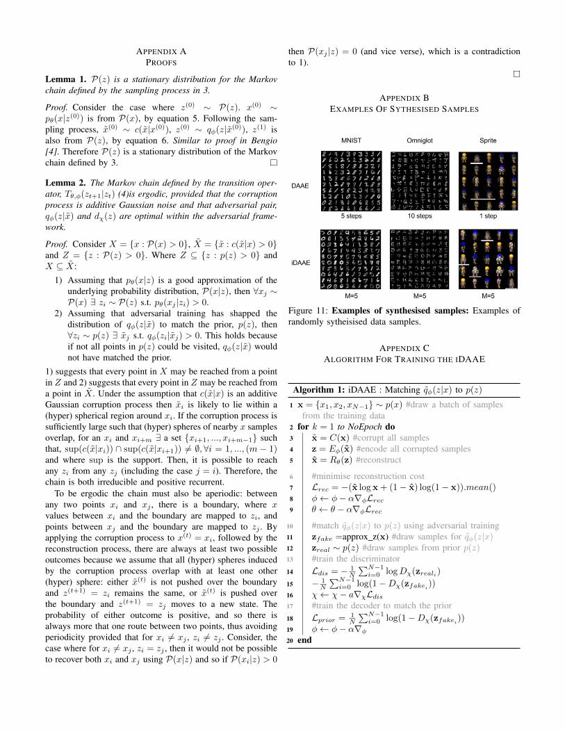
APPENDIX BEXAMPLES OF SYTHESISED SAMPLES

Figure 11: Examples of synthesised samples: Examples ofrandomly sytheisised data samples.

APPENDIX CALGORITHM FOR TRAINING THE IDAAE

Algorithm 1: iDAAE : Matching qφ(z|x) to p(z)

1 x = {x1, x2, xN−1} ∼ p(x) #draw a batch of samplesfrom the training data

2 for k = 1 to NoEpoch do3 x = C(x) #corrupt all samples4 z = Eφ(x) #encode all corrupted samples5 x = Rθ(z) #reconstruct

6 #minimise reconstruction cost7 Lrec = −(x logx+ (1− x) log(1− x)).mean()8 φ← φ− α∇φLrec9 θ ← θ − α∇φLrec

10 #match qφ(z|x) to p(z) using adversarial training11 zfake =approx z(x) #draw samples for qφ(z|x)12 zreal ∼ p(z) #draw samples from prior p(z)13 #train the discriminator14 Ldis = − 1

N

∑N−1i=0 logDχ(zreali)

15 − 1N

∑N−1i=0 log(1−Dχ(zfakei))

16 χ← χ− a∇χLdis17 #train the decoder to match the prior18 Lprior = 1

N

∑N−1i=0 log(1−Dχ(zfakei))

19 φ← φ− α∇φ20 end

Algorithm 2: Drawing samples from qφ(z|x)1 function: approx z({x1, x2, ...xN−1})2 for i = 0 to N − 1 do3 zi = [ ]4 for j = 1 to M do5 xi,j = C(xi)6 zi,j = Eφ(xj)7 end8 zi.append(

1M

∑Mj=1 zj)

9 end10 return z = {z1, z2...zN−1}

APPENDIX DALGORITHM FOR MONTE CARLO INTEGRATION

APPENDIX EMNIST RESULTS

A. Datasets: MNIST

The MNIST dataset consists of grey-scale images of hand-written digits between 0 and 9, with 50k training samples,10k validation samples and 10k testing samples. The training,validation and testing dataset have an equal number of samplesfrom each category. The samples are 28-by-28 pixels. TheMNIST dataset is a simple dataset with few classes and manytraining examples, making it a good dataset for proof-of-concept. However, because the dataset is very simple, it doesnot necessarily reveal the effects of subtle, but potentiallyimportant, changes to algorithms for training or sampling. Forthis reason, we consider two datasets with greater complexity.

B. Architecture and Training: MNIST

For the MNIST dataset, we train a total of 5 models detailedin Table III. The encoder, decoder and discriminator networkseach have two fully connected layers with 1000 neurons each.For most models the size of the encoding is 10 units, and theprior distribution that the encoding is being matched to is a10D Gaussian. All networks are trained for 100 epochs on thetraining dataset, with a learning rate of 0.0002 and a batchsize of 64. The standard deviation of the additive Gaussiannoise used during training is 0.5 for all iDAAE and DAAEmodels.

An additional DAAE model is trained using the sametraining parameters and networks as described above but with amixture of 10 2D Gaussians for the prior. Each 2D Gaussianwith standard deviation 0.5 is equally spaced with its meanaround a circle of radius 4 units. This results in a prior with10 modes separated from each other by large regions of verylow probability. This model of the prior is very unrealistic, asit assumes that MNIST digits occupy distinct regions of imageprobability space. In reality, we may expect two numbersthat are similar to exist side by side in image probabilityspace, and for there to exist a smooth transition betweenhandwritten digits. As a consequence of this, this model isintended specifically for evaluating how well the posterior

Table III: Models trained on MNIST: 5 models are trainedon the MNIST dataset. Corruption indicates the standard de-viation of Gaussian noise added during the corruption process,c(x|x). Prior indicated the prior distribution imposed on thelatent space. M is the number of Monte Carlo integration steps(see Algorithm 2 in Appendix) used during training - thisapplies only to the iDAAE.

ID Model Corruption Prior M

1 AAE 0.0 10D Gaussian -2 DAAE 0.5 10D Gaussian -3 DAAE 0.5 10-GMM -4 iDAAE 0.5 10D Gaussian 55 iDAAE 0.5 10D Gaussian 25

Table IV: MNIST Reconstruction: Recon. shows the meansquared error for reconstructions of corrupted test data samplesaccompanied by the standard error. Corruption is the standarddeviation of the additive Gaussian noise used during trainingand testing.

Model & Training Recon.

Model Corruption Prior M Mean ± s.e.

AAE 0.0 10D Gaussian - 0.017±0.001DAAE 0.5 10D Gaussian - 0.023±0.001DAAE 0.5 2D 10-GMM - 0.043±0.001iDAAE 0.5 10D Gaussian 5 0.022±0.001iDAAE 0.5 10D Gaussian 25 0.026±0.001

distribution over latent space may be matched to a mixtureof Gaussians - something that could not be achieved easily bya VAE [14].

C. Reconstruction: MNIST

Table IV shows reconstruction error on samples fromthe testing dataset, for each of the models trained on theMNIST training dataset. Reconstruction error for the DAAEand iDAAE trained with a 10D Gaussian prior do not out-perform the AAE. However, the reconstruction task for theAAE model was less challenging than that of the DAAE andiDAAE models because samples were not corrupted beforethe encoding step. The best model for reconstruction wasthe iDAAE with M = 5, increasing M to 25 led to worsereconstruction error, as reconstructions tended to appear morelike mean samples.

Reconstruction error for the DAAE trained using a 2Dmixture of 10 Gaussians under-performed compared to the restof the models. All reconstructions looked like mean images,which may be expected given the nature of the prior.

D. Sampling: MNIST

To calculate the log-likelihood of samples drawn fromDAAE, iDAAE and AAE models trained on the MNISTdataset, a Parzen window is fitted to 1×104 generated samplesfrom a single trained model. The bandwidth for constructingthe Parzen window was selected by choosing one of 10values, evenly space along a log axis between −1 and 0,

that maximises the likelihood on a validation dataset. Thelog-likelihood for each model was then evaluated on the testdataset.

Table V shows the log-likelihood on the test dataset forsamples drawn from models trained on the MNIST trainingdataset. First, we will discuss models trained with a 10DGaussian prior. The best log-likelihood was achieved by theiDAAE with M = 5. Synthesised samples generated by MCsampling from the DAAE model caused the log-likelihood todecrease. This may be because the samples tended towardsmean samples, dropping modes, causing the log-likelihood todecrease. Initial samples and those obtained after 5 iterationsof sampling are shown in Figure 12. The samples in 12(d)are clearer than in 12(c). Although mode-dropping is notimmediately apparent, note that the digit 4 is not present after5 iterations.

Now, we consider the DAAE model trained with a 2D, 10-GMM prior. Samples drawn from the prior are shown in Figure13(a). The purpose of this experiment was to show the effectsof MC sampling, where the distribution from which initialsamples of z0 are drawn is significantly different to the prior.Samples of z0 were drawn from a normal distribution andpassed through the decoder of the DAAE model to produceinitial image samples, see Figure 13(c). A further 9 steps ofMC sampling were applied to synthesise the samples shownin Figure 13(d). As expected, the initial image samples donot look like MNIST digits, and MC sampling improvessamples dramatically. Unfortunately however, many of thesamples appear to correspond to samples at modes of the datadistribution. In addition, several modes appear to be missingfrom the model distribution. This may be attributed to thenature of the prior, since we did not encounter this problem tothe same extent when using a 10D Gaussian prior (see Figure12).

Synthesising MNIST samples is fairly trivial, since there aremany training examples and few classes. For this reason, it isdifficult to see the benefits of using DAAE or iDAAE modelscompared to AAE models. Now, we focus on the two morecomplex datasets, Omniglot and Sprites. We find that iDAAEmodels and correctly sampled DAAE models may be usedto synthesise samples with higher log-likelihood than samplessynthesised using an AAE.

1) Classification: MNIST: The MNIST dataset consists of10 classes, [0, 9], the classification task involves correctlypredicting a label in this interval. For the MNIST dataset, theSVM classifier is trained on encoded samples from the MNISTtraining dataset and evaluated on encoded samples from theMNIST testing dataset, results are shown in Table VI.

First, we consider the results for DAAE, iDAAE and AAEmodels trained with a 10D Gaussian prior. Classifiers trainedon encodings extracted from the encoders of trained DAAE,iDAAE or AAE models out-performed classifiers trained onPCA of image samples. Classifiers trained on the encodingsextracted from the encoders of learned DAAE and iDAAEmodels out-performed those trained on the encodings extractedfrom the encoders of the AAE model.

(a) Prior (one channel) (b) Latent samples

(c) x(0) (d) x(5)

Figure 12: MNIST Markov chain (MC) sampling: Onechannel of the 10D Gaussian Prior a) One channel of the10D Gaussian prior used to train the DAAE. b) Samples drawnfrom qφ(z|x), projected in to 2D space, and colour coded bythe digit labels. c) Initial samples, x(0) generated by a normaldistribution. d) Corresponding samples after 5 iterations ofMC sampling. Notice how the highlighted “1” changes to a“2” after 5 iterations of MC sampling.

(a) 2D Gaussian Mixture prior (b) Latent samples

(c) x(0) (d) x(9)

Figure 13: MNIST Markov chain (MC) sampling: a) 2DGaussian Mixture prior used to train a DAAE. b) Samplesdrawn from qφ(z|x) projected into 2D space using PCAand colour coded by the digit labels. c) Initial sample, x(0),generated by a normal distribution. d) Corresponding samplesgenerated after 9 further iterations of MC sampling.

Table V: MNIST log-likelihood of pθ(x): To calculate thelog-likelihood of pθ(x), a Parzen window was fit to 104

generated samples and the mean likelihood was reported fora testing data set. The bandwidth used for the Parzen windowwas determined using a validation set. The training, test andvalidation datasets had different samples.

Model & Training Log-likelihood

Model Corruption Prior M x(0) x(5)

AAE 0.0 10D Gaussian - 529 -DAAE 0.5 10D Gaussian - 529 444DAAE 0.5 2D 10-GMM - 9 205iDAAE 0.5 10D Gaussian 5 532 -iDAAE 0.5 10D Gaussian 25 508 -

Table VI: MNIST Classification: SVM classifiers with RBFkernels were trained on encoded MNIST training data samples.The samples were encoded using the encoder of the trainedAAE, DAAE or iDAAE models. Classification scores aregiven for the MNIST test dataset.

Model & Training AccuracyModel Corruption Prior M %

AAE 0.0 10D Gaussian - 95.19%DAAE 0.5 10D Gaussian - 95.28%DAAE 0.5 2D 10-GMM - 73.81%iDAAE 0.5 10D Gaussian 5 96.48%iDAAE 0.5 10D Gaussian 25 96.24%PCA + SVM 94.73%

The differences in classification score for each model on theMNIST dataset are small; this might be because it is relativelyeasy to classify MNIST digits with very high accuracy [29].We turn now to a more complicated dataset, the Omniglotdataset, to better show the benefits of using denoising whentraining adversarial autoencoders.

APPENDIX FDETAILS FOR CALCULATING LOG-LIKELIHOOD

A. Omniglot

To calculate log-likelihood of samples, a Parzen windowwas fit to 1× 103 synthesised samples, where the bandwidthwas determined on the testing dataset in a similar way to thatin Section E-D. The log-likelihood was evaluated on both theevaluation dataset, and the testing dataset. To compute the log-likelihood on the of the testing dataset a Parzen window wasfit to a new set of synthesized samples, different to those usedto calculate the bandwidth. The results are shown in Figure 3.

B. Sprites

To calculate log-likelihood of samples, a Parzen windowwas fit to 1×103 synthesized samples. The bandwidth was setas previously described in Section E-D; we found the optimalbandwidth to be 1.29.

APPENDIX GIDAAE ROBUSTNESS TO HYPER PARAMETERS

Figure 14: iDAAE

Figure 15: Robustness to hyper parameters