Denoising and Demosaicking of Color

Images

by

Mina Rafi Nazari

Thesis submitted to the

Faculty of Graduate and Postdoctoral Studies

In partial fulfillment of the requirements

For the Ph.D. degree in

Electrical and Computer Engineering

School of Electrical Engineering and Computer Science

Faculty of Engineering

University of Ottawa

c© Mina Rafi Nazari, Ottawa, Canada, 2017

Abstract

Most digital cameras capture images through Color Filter Arrays (CFA), and recon-

struct the full color image from the CFA image. Each CFA pixel only captures one primary

color component at each pixel location; the other primary components will be estimated

using information from neighboring pixels. During the demosaicking algorithm, the un-

known color components will be estimated at each pixel location. Most of the demosaicking

algorithms use the RGB Bayer CFA pattern with Red, Green and Blue filters.

Some other CFAs contain four color filters. The additional filter is a panchromatic/white

filter, and it usually receives the full light spectrum. In this research, we studied and com-

pared different four channel CFAs with panchromatic/white filter, and compared them

with three channel CFAs. An appropriate demosaicking algorithm has been developed for

each CFA. The most well-known three-channel CFA is Bayer. The Fujifilm X-Trans pattern

has been studied in this work as another three-channel CFA with a different structure.

Three different four-channel CFAs have been discussed in this research: RGBW-Kodak,

RGBW-Bayer and RGBW- 5×5. The structure and the number of filters for each color are

different for these CFAs. Since the Least-Square Luma-Chroma Demultiplexing method is

a state of the art demosaicking method for the Bayer CFA, we designed the Least-Square

method for RGBW CFAs. The effect of noise on different CFA patterns will be discussed

for four channel CFAs. The Kodak database has been used to evaluate our non-adaptive

and adaptive demosaicking methods as well as the optimized algorithms with the least

square method.

The captured values of white (panchromatic/clear) filters in RGBW CFAs have been

estimated using red, green and blue filter values. Sets of optimized coefficients have been

proposed to estimate the white filter values accurately. The results have been validated

using the actual white values of a hyperspectral image dataset.

A new denoising-demosaicking method for RGBW-Bayer CFA has been presented in

this research. The algorithm has been tested on the Kodak dataset using the estimated

value of white filters and a hyperspectral image dataset using the actual value of white

ii

filters, and the results have been compared. The results in both cases have been compared

with the previous works on RGB-Bayer CFA, and it shows that the proposed algorithm

using RGBW-Bayer CFA is working better than RGB-Bayer CFA in presence of noise.

iii

Acknowledgements

I would like to take this opportunity to thank my PhD supervisor, professor Eric Dubois,

for his help and support throughout these years. His constant support, his advice in every

steps of my degree and his deep knowledge helped me through this path. I would always

be thankful for his supervision during my PhD degree.

Also I would like to thank all the committee members of my defense session, in addition

to all my friends in the VIVA lab who have provided a friendly environment for research.

I would like to extend my gratitude to the kind staff of the engineering department at

the University of Ottawa and my dear friends in the city of Ottawa.

I would like to thank my brother, for his kind support through my undergraduate and

graduate studies. I was very fortunate to have him around during tough times of my PhD.

Last but not least, special thanks to my dear family which without their kind supports

the completion of this work would not be imaginable.

iv

Dedication

To my parents, my grandparents and my uncle, who always gave their unconditional

love and support to me.

v

Table of Contents

List of Tables ix

List of Figures xiii

1 Introduction 1

1.1 Problem Statement . . . . . . . . . . . . . . . . . . . . . . . . . . . . . . . 1

1.2 State of the art . . . . . . . . . . . . . . . . . . . . . . . . . . . . . . . . . 2

1.3 Research hypothesis and objectives . . . . . . . . . . . . . . . . . . . . . . 4

1.4 Proposed research . . . . . . . . . . . . . . . . . . . . . . . . . . . . . . . . 6

1.5 Structure of the thesis . . . . . . . . . . . . . . . . . . . . . . . . . . . . . 8

2 Background and Related Work 9

2.1 Representation of CFA formation . . . . . . . . . . . . . . . . . . . . . . . 9

2.2 General methods for demosaicking . . . . . . . . . . . . . . . . . . . . . . . 13

2.2.1 Interpolation techniques . . . . . . . . . . . . . . . . . . . . . . . . 14

2.2.2 Edge-directed interpolation . . . . . . . . . . . . . . . . . . . . . . 15

2.2.3 Demosaicking methods using wavelet . . . . . . . . . . . . . . . . . 15

2.2.4 Demosaicking based on the frequency domain representation . . . . 16

2.3 Image quality measurement . . . . . . . . . . . . . . . . . . . . . . . . . . 17

vi

2.3.1 Peak Signal-to-Noise Ratio . . . . . . . . . . . . . . . . . . . . . . . 17

2.3.2 S-CIELAB . . . . . . . . . . . . . . . . . . . . . . . . . . . . . . . . 18

2.4 Review of different CFA patterns . . . . . . . . . . . . . . . . . . . . . . . 19

2.4.1 Three channel CFAs . . . . . . . . . . . . . . . . . . . . . . . . . . 19

2.4.2 Four channel CFAs . . . . . . . . . . . . . . . . . . . . . . . . . . . 21

2.5 Noise effect on CFA image . . . . . . . . . . . . . . . . . . . . . . . . . . . 23

2.5.1 Demosaicking methods with a noise reduction stage . . . . . . . . . 24

2.5.2 State of art joint demosaicking-denoising method for noisy RGB-

Bayer patterns . . . . . . . . . . . . . . . . . . . . . . . . . . . . . 26

2.6 Summary . . . . . . . . . . . . . . . . . . . . . . . . . . . . . . . . . . . . 27

3 Demosaicking algorithms in the noise-free case 28

3.1 Demosaicking algorithm structure . . . . . . . . . . . . . . . . . . . . . . . 28

3.2 Three channel color filter array . . . . . . . . . . . . . . . . . . . . . . . . 33

3.3 Demosaicking for the Fujifilm X-Trans pattern . . . . . . . . . . . . . . . . 33

3.4 Four channel color filter array . . . . . . . . . . . . . . . . . . . . . . . . . 52

3.4.1 RGBW-Kodak pattern . . . . . . . . . . . . . . . . . . . . . . . . . 54

3.4.2 RGBW - 5× 5 pattern . . . . . . . . . . . . . . . . . . . . . . . . . 63

3.4.3 RGBW-Bayer pattern . . . . . . . . . . . . . . . . . . . . . . . . . 68

3.4.4 Comparison between RGBW patterns . . . . . . . . . . . . . . . . . 75

3.4.5 White filter estimation . . . . . . . . . . . . . . . . . . . . . . . . . 82

3.4.6 Least-square method optimization algorithm . . . . . . . . . . . . . 94

3.5 Four-channel CFA reconstruction using hyperspectral images . . . . . . . . 99

3.5.1 Spectral image dataset . . . . . . . . . . . . . . . . . . . . . . . . . 99

3.5.2 RGBW CFA reconstruction using hyperspectral images . . . . . . . 101

3.5.3 Results . . . . . . . . . . . . . . . . . . . . . . . . . . . . . . . . . . 103

vii

4 Demosaicking of noisy CFA images 109

4.1 Noise in CFA images . . . . . . . . . . . . . . . . . . . . . . . . . . . . . . 109

4.2 Noise estimation . . . . . . . . . . . . . . . . . . . . . . . . . . . . . . . . 111

4.3 Demosaicking of noisy CFA images . . . . . . . . . . . . . . . . . . . . . . 115

4.3.1 Luma noise reduction using BM3D . . . . . . . . . . . . . . . . . . 118

4.4 Results . . . . . . . . . . . . . . . . . . . . . . . . . . . . . . . . . . . . . . 118

5 Conclusion 135

5.1 Conclusions . . . . . . . . . . . . . . . . . . . . . . . . . . . . . . . . . . . 135

5.2 Future work . . . . . . . . . . . . . . . . . . . . . . . . . . . . . . . . . . . 137

References 138

viii

List of Tables

3.1 PSNR of Kodak images using Bayer and Fujifilm X-Trans patterns.(a) RGB-

Bayer (Least-Square method), (b) Fujifilm (Non Adaptive demosaicking),

(c) Fujifilm (Adaptive demosaicking), (d) Fujifilm (Bayer-like Adaptive de-

mosaicking), (e) Fujifilm (Least-Square method) . . . . . . . . . . . . . . . 50

3.2 S-CIELAB of Kodak images using Bayer and Fujifilm X-Trans patterns.(a)

RGB-Bayer (Least-Square method), (b) Fujifilm (Non Adaptive demosaick-

ing), (c) Fujifilm (Adaptive demosaicking), (d) Fujifilm (Bayer-like Adaptive

demosaicking), (e) Fujifilm (Least-Square method) . . . . . . . . . . . . . . 51

3.3 PSNR of Kodak images using RGB-Bayer (least-square method) and RGBW-

Kodak (Non-adaptive and Revised method) and the average PSNR over 24

Kodak images . . . . . . . . . . . . . . . . . . . . . . . . . . . . . . . . . . 61

3.4 S-CIELAB of Kodak images using RGB-Bayer (least-square method) and

RGBW-Kodak (Non-adaptive and Revised method) and the average S-

CIELAB over 24 Kodak images . . . . . . . . . . . . . . . . . . . . . . . . 62

3.5 PSNR of proposed Non-Adaptive demosaicking method using RGBW(5×5)

pattern and the presented method in [45] for Kodak dataset . . . . . . . . 67

3.6 Comparison between the PSNR of Adaptive demosaicking method using

RGBW-Bayer CFA and Least Square method using RGB-Bayer for Kodak

dataset . . . . . . . . . . . . . . . . . . . . . . . . . . . . . . . . . . . . . . 73

3.7 Comparison between the S-CIELAB of Adaptive demosaicking method using

RGBW-Bayer and Least Square method using RGB-Bayer for Kodak dataset 74

ix

3.8 PSNR for Non-Adaptive demosaicking method using different RGBW pat-

terns and the average PSNR over 24 Kodak images . . . . . . . . . . . . . 77

3.9 S-CIELAB of some sample images for Non-Adaptive demosaicking method

using different RGBW patterns and the average S-CIELAB over 24 Kodak

images . . . . . . . . . . . . . . . . . . . . . . . . . . . . . . . . . . . . . . 78

3.10 Comparison between the PSNR of Kodak images for adaptive demosaicking

method using RGBW CFAs and least-square method using RGB-Bayer . . 80

3.11 Comparison between the S-CIELAB of Kodak images for demosaicking method

using RGBW CFAs and least-square method using RGB-Bayer . . . . . . . 81

3.12 PSNR Kodak images and average total PSNR over 24 images. (a) Results of applying

adaptive demosaicking method designed using equation 3.90 for the CFA modeled using

equation 3.90, (b) Results of applying adaptive demosaicking method designed using

equation 3.90 for the CFA modeled using equation 3.135, (c) Results of applying adaptive

demosaicking method designed using equation 3.135 for the CFA modeled using equation

3.135 . . . . . . . . . . . . . . . . . . . . . . . . . . . . . . . . . . . . . . . 92

3.13 S-CIELAB for Kodak images and average total S-CIELAB over 24 images. (a) Results

of applying adaptive demosaicking method designed using equation 3.90 for the CFA

modeled using equation 3.90, (b) Results of applying adaptive demosaicking method

designed using equation 3.90 for the CFA modeled using equation 3.135, (c) Results

of applying adaptive demosaicking method designed using equation 3.135 for the CFA

modeled using equation 3.135 . . . . . . . . . . . . . . . . . . . . . . . . . . . . 93

3.14 Comparison between the PSNR of Kodak images for Least-Square demo-

saicking method using Bayer-RGBW CFA and VEML6040 and KAI-Kodak11002

sensors and Least Square method using RGB-Bayer . . . . . . . . . . . . . 97

3.15 Comparison between the S-CIELAB of Kodak images for Least-Square de-

mosaicking method using Bayer-RGBW CFA and VEML6040 and KAI-

Kodak11002 sensors and Least Square method using RGB-Bayer . . . . . . 98

x

3.16 Comparison between the PSNR of hyperspectral images [33] for Least Square demosaick-

ing method using RGBW-Bayer using VEML6040 sensor and Least Square method using

RGB-Bayer . . . . . . . . . . . . . . . . . . . . . . . . . . . . . . . . . . . . 104

3.17 Comparison between the PSNR of hyperspectral images [33] for Least Square demosaick-

ing method using RGBW-Bayer using KAI-Kodak 11002 sensor and Least Square method

using RGB-Bayer . . . . . . . . . . . . . . . . . . . . . . . . . . . . . . . . . 105

3.18 PSNR of estimated white using equation (3.135) pixels and actual white

pixels for 30 hyperspectral images using VEML6040 sensor . . . . . . . . . 107

3.19 PSNR of estimated white using equation (3.136) pixels and actual white

pixels for 30 hyperspectral images using KAI-Kodak11002 sensor . . . . . . 108

4.1 Average PSNR over 24 Kodak images using least-Square (LS) method and

demosaicking-denoising method on RGBW-Bayer using VEML6040 sensor

and RGB-Bayer for different noise levels . . . . . . . . . . . . . . . . . . . 120

4.2 Average S-CIELAB over 24 Kodak images using least-Square(LS) method

and demosaicking-denoising method on RGBW-Bayer using VEML6040 sen-

sor for different noise levels . . . . . . . . . . . . . . . . . . . . . . . . . . . 121

4.3 Average PSNR over 24 Kodak images using least-Square(LS) method and

demosaicking-denoising method on RGBW-Bayer using Kodak-KAI-11000

sensor and RGB-Bayer for different noise levels . . . . . . . . . . . . . . . 122

4.4 Average S-CIELAB over 24 Kodak images using least-Square(LS) method

and demosaicking-denoising method on RGBW-Bayer using Kodak-KAI-

11000 sensor for different noise levels . . . . . . . . . . . . . . . . . . . . . 123

4.5 Average PSNR over 30 hyperspectral images using demosaicking-denoising

method on RGBW-Bayer using VEML6040 and RGB-Bayer for different

noise levels . . . . . . . . . . . . . . . . . . . . . . . . . . . . . . . . . . . . 128

4.6 Average PSNR over 30 hyperspectral images using demosaicking-denoising

method on RGBW-Bayer using Kodak-KAI-11000 and RGB-Bayer for dif-

ferent noise levels . . . . . . . . . . . . . . . . . . . . . . . . . . . . . . . . 129

xi

4.7 Average S-CIELAB over 30 hyperspectral images using demosaicking-denoising

method on RGBW-Bayer using VEML6040 and RGB-Bayer for different

noise levels . . . . . . . . . . . . . . . . . . . . . . . . . . . . . . . . . . . . 132

4.8 Average S-CIELAB over 30 hyperspectral images using demosaicking-denoising

method on RGBW-Bayer using Kodak-KAI-11000 and RGB-Bayer for dif-

ferent noise levels . . . . . . . . . . . . . . . . . . . . . . . . . . . . . . . . 133

xii

List of Figures

1.1 CFA spatial multiplexing of red, green and blue sub-samples for the Bayer

pattern . . . . . . . . . . . . . . . . . . . . . . . . . . . . . . . . . . . . . . 2

1.2 Sample CFA patterns . . . . . . . . . . . . . . . . . . . . . . . . . . . . . . 5

2.1 Bayer CFA sampling structure shows the constituent sampling structures

ΨR ( ◦), ΨG (4) and ΨB (�). . . . . . . . . . . . . . . . . . . . . . . . . . 10

2.2 Bilinear interpolation for green components for the Bayer pattern . . . . . 14

2.3 Bilinear interpolation for red/ blue components for the Bayer pattern . . . 14

2.4 Bayer CFA pattern . . . . . . . . . . . . . . . . . . . . . . . . . . . . . . . 20

2.5 Fujifilm X-Trans CFA pattern . . . . . . . . . . . . . . . . . . . . . . . . . 20

2.6 Diagonal Stripe CFA pattern . . . . . . . . . . . . . . . . . . . . . . . . . . 21

2.7 CYYM CFA pattern . . . . . . . . . . . . . . . . . . . . . . . . . . . . . . 21

2.8 RGBE CFA pattern . . . . . . . . . . . . . . . . . . . . . . . . . . . . . . . 22

2.9 RGBW-Bayer CFA pattern . . . . . . . . . . . . . . . . . . . . . . . . . . 22

2.10 CYGM CFA pattern . . . . . . . . . . . . . . . . . . . . . . . . . . . . . . 23

3.1 Fujifilm X-Trans CFA pattern . . . . . . . . . . . . . . . . . . . . . . . . . 34

3.2 Luma- Chroma position for Fujifilm X-Trans pattern . . . . . . . . . . . . 37

3.3 Fujifilm adaptive demosaicking system . . . . . . . . . . . . . . . . . . . . 39

xiii

3.4 Comparison between The new method using X-Trans and LSLCD method

using Bayer . . . . . . . . . . . . . . . . . . . . . . . . . . . . . . . . . . . 49

3.5 Sample four channel CFA patterns . . . . . . . . . . . . . . . . . . . . . . 53

3.6 An 8× 8 section of the Kodak-RGBW pattern showing four periods . . . . 54

3.7 Luma- Chroma position in one unit cell for RGBW-Kodak pattern . . . . . 57

3.8 Comparison between the revised method using RGBW-Kodak and LSLCD

method using RGB-Bayer . . . . . . . . . . . . . . . . . . . . . . . . . . . 60

3.9 RGBW(5× 5)[45] (four periods) . . . . . . . . . . . . . . . . . . . . . . . . 63

3.10 The smaller repeated pattern in RGBW(5× 5) . . . . . . . . . . . . . . . . 64

3.11 Luma- Chroma position in one unit cell-RGBW(5× 5) . . . . . . . . . . . 66

3.12 RGBW-Bayer pattern . . . . . . . . . . . . . . . . . . . . . . . . . . . . . 68

3.13 Luma- Chroma position in one unit cell for RGBW-Bayer . . . . . . . . . . 70

3.14 Comparison between The adaptive and non-adaptive demosaicking method

for different four channel CFAs . . . . . . . . . . . . . . . . . . . . . . . . 76

3.15 Non-normalized spectral response of red, green, blue and white color filters

for VEML6040 sensor (400nm-800nm) . . . . . . . . . . . . . . . . . . . . 83

3.16 Non-normalized spectral response of red, green and blue color filters for

KAI-Kodak11002 sensor (400nm-800nm) . . . . . . . . . . . . . . . . . . . 84

3.17 Non-normalized spectral response of white filter for KAI-Kodak11002 sensor

(400nm-800nm) . . . . . . . . . . . . . . . . . . . . . . . . . . . . . . . . . 85

3.18 Sample spectral images from [33] . . . . . . . . . . . . . . . . . . . . . . . 100

4.1 Eight different masks for homogeneity measures with the size ω = 5 . . . . 113

4.2 Demosaicking-denoising system . . . . . . . . . . . . . . . . . . . . . . . . 116

4.3 Added noise level versus estimated noise level on Kodak image dataset using

VEML6040 . . . . . . . . . . . . . . . . . . . . . . . . . . . . . . . . . . . 117

xiv

4.4 Reconstructed noisy image with σ = 6 using regular least-square demosaick-

ing method and denoising-demosaicking method with RGBW-Bayer CFA . 125

4.5 Reconstructed noisy image with σ = 14 using regular least-square demo-

saicking method and denoising-demosaicking method with RGBW-Bayer CFA126

4.6 Comparison between the average PSNR over 30 hyperspectral images us-

ing demosaicking-denoising method on RGBW-Bayer with VEML6040 and

RGB-Bayer for different noise levels . . . . . . . . . . . . . . . . . . . . . . 130

4.7 Comparison between the average PSNR over 30 hyperspectral images us-

ing demosaicking-denoising method on RGBW-Bayer with Kodak-KAI11000

and RGB-Bayer for different noise levels . . . . . . . . . . . . . . . . . . . 131

4.8 Added noise level versus estimated noise level on hyperspectral image dataset

using VEML6040 . . . . . . . . . . . . . . . . . . . . . . . . . . . . . . . . 134

xv

Chapter 1

Introduction

1.1 Problem Statement

Imaging systems need three primary color coordinate values (tristimulus values) at each

pixel location to reconstruct a full color image. Digital cameras usually capture images

through a Color Filter Array (CFA). CFAs filter the incident light at each pixel sensor

element with one of a certain number of color filters (usually three), and thus the captured

image contains only one color component at each pixel, while the other components are

missing. Through the demosaicking process, the missing color components at each pixel

will be estimated and the full color image will be reconstructed.

CFAs vary based on their color filters, the number of sensor classes (different filters)

in the CFA pattern, and their geometric structure. Most of the CFAs contain the three

display primary colors (red, green and blue), while some others contain cyan, magenta and

yellow. There are also some CFAs with an additional transparent filter. The arrangement

of the color filters is different in each pattern, as well as the number of red, green, blue or

other pixels in one period of the structure. The most common CFA is the Bayer structure

containing two green pixels, one red and one blue in each template. See Figure 1.2 for

some examples of CFA patterns.

Demosaicking refers to the process of reconstructing an image from incomplete samples.

1

The most basic demosaicking scheme relies on simple interpolation between neighboring

pixel information within each class and its results are usually not adequate [2]. The per-

formance of the demosaicking algorithm using different patterns and the robustness of the

algorithm to noise are two major challenges in this field.

1.2 State of the art

Demosaicking algorithms and CFA design methods are both crucial steps to restore

the image. In previous research, the demosaicking algorithms were mainly analyzed and

implemented in the spatial domain. Demosaicking techniques in the spatial domain are

categorized into two major groups. The first set of methods contains fixed interpolation

techniques such as nearest neighbor, bilinear interpolation and bicubic interpolation on

each color channel. Figure 1.1 shows the spatial multiplexing of sub-samples for the Bayer

pattern. These methods usually provide satisfactory demosaicking results in smooth areas,

but the results are not well estimated along edges or in high frequency areas. The second

set of methods use inter-channel correlation with assumptions like smooth hue transition.

Figure 1.1: CFA spatial multiplexing of red, green and blue sub-samples for the Bayer

pattern

As will be shown later, the CFA signal can be analyzed in the frequency domain, where

it can be interpreted as the frequency division multiplexing of a baseband grayscale com-

ponent called luma and color components at high spatial frequency referred to as chroma

components. The number of chromas usually depend on the number of pixels/ filters in one

period of the CFA pattern. The specific chroma in the low frequency band is called luma

2

or brightness component. The CFA signal can be modeled as a sum of one luma and a

set of chromas at specific spatial frequencies. In the last decade, it has been demonstrated

that the luma and chroma components are reasonably isolated in the frequency domain.

Hence, demosaicking algorithms using a frequency domain representation became more

competitive.

The most popular and simple CFA template is Bayer, and many existing demosaicking

methods are working well on it. One of the best demosaicking methods for RGB-Bayer

pattern in the frequency domain which outperforms other methods, is the adaptive least

square luma-chroma demultiplexing method. In this method a set of least-square filters will

be applied on an adaptive demosaicking method. The adaptive demosaicking algorithm for

the Bayer pattern chooses one chroma component that locally has less overlap with luma,

and reconstructs the other chromas adaptively. Some literature has proposed that using

other patterns rather than Bayer might lead to better reconstruction results. Due to the

overlapping effect between different channels in the CFA, some CFA structures might work

better than Bayer. Some patterns have been proposed but they have not been fully studied,

like the Fujifilm X-Trans pattern. Some others proposed and commercially implemented

that use other color filters rather than red, green and blue might provide better signal to

noise ratio.

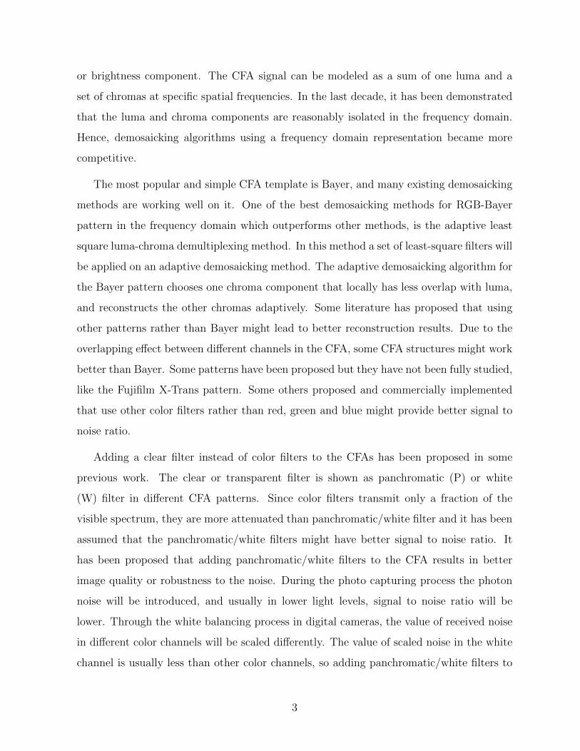
Adding a clear filter instead of color filters to the CFAs has been proposed in some

previous work. The clear or transparent filter is shown as panchromatic (P) or white

(W) filter in different CFA patterns. Since color filters transmit only a fraction of the

visible spectrum, they are more attenuated than panchromatic/white filter and it has been

assumed that the panchromatic/white filters might have better signal to noise ratio. It

has been proposed that adding panchromatic/white filters to the CFA results in better

image quality or robustness to the noise. During the photo capturing process the photon

noise will be introduced, and usually in lower light levels, signal to noise ratio will be

lower. Through the white balancing process in digital cameras, the value of received noise

in different color channels will be scaled differently. The value of scaled noise in the white

channel is usually less than other color channels, so adding panchromatic/white filters to

3

the CFA might increase the overall signal to noise ratio in the image. Several patterns

with clear filters have been proposed in literature, and the noise effect of these patterns

needs to be fully studied.

1.3 Research hypothesis and objectives

Advanced demosaicking algorithms have been discussed in the literature for some three

channel CFAs like Bayer. We propose that luma-chroma demultiplexing methods can be

used to design good demosaicking methods for various other RGB CFAs such as Fujifilm

X-Trans pattern.

Different types of four-channel RGBW CFAs have been introduced in previous work.

The comparison between RGBW CFAs and the three-channel RGB CFAs, indicated that

the quality of image and signal to noise ratio (SNR) were improved using the RGBW CFAs.

We hypothesize that better overall image quality can be obtained for noisy camera sensor

images using RGBW patterns, since the panchromatic/white filters pass more light, and

therefore result in better signal to noise ratio. A basic demosaicking algorithm for different

RGBW CFAs can be designed, and Luma-chroma demultiplexing methods can be used to

design optimized demosaicking methods for noisy image with RGBW CFAs.

The objectives of this research are:

• To design demosaicking method based on the frequency domain analysis for three

channel Fujifilm X-Trans pattern that have not been studied in the literature.

• To develop demosaicking systems for RGBW CFAs that demonstrate that RGBW

CFAs have better performance in the presence of noise than RGB Bayer CFAs.

• To present a general method that can be used for luma-chroma demultiplexing with

advanced RGB and RGBW CFA designs.

4

(a) RGB-Bayer pattern

(b) CYYM pattern

(c) RGBW-Bayer pattern

(d) RGBW-Kodak pattern

(e) Fujifilm X-Trans pattern

Figure 1.2: Sample CFA patterns

5

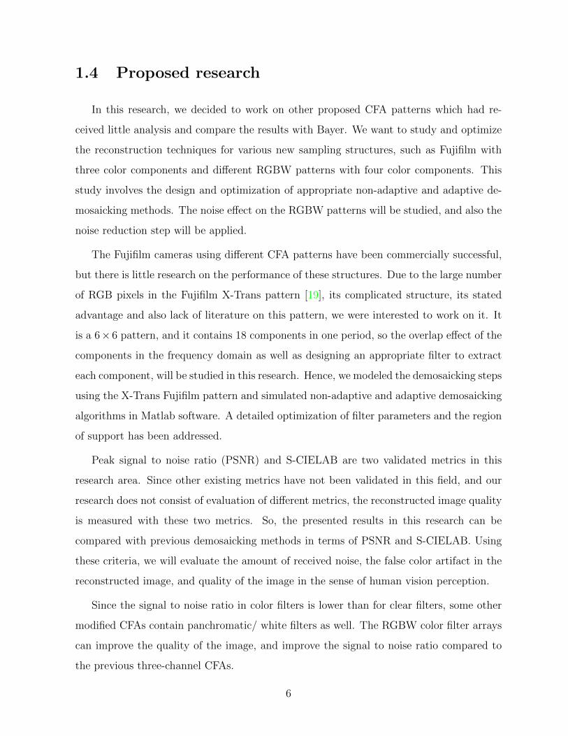
1.4 Proposed research

In this research, we decided to work on other proposed CFA patterns which had re-

ceived little analysis and compare the results with Bayer. We want to study and optimize

the reconstruction techniques for various new sampling structures, such as Fujifilm with

three color components and different RGBW patterns with four color components. This

study involves the design and optimization of appropriate non-adaptive and adaptive de-

mosaicking methods. The noise effect on the RGBW patterns will be studied, and also the

noise reduction step will be applied.

The Fujifilm cameras using different CFA patterns have been commercially successful,

but there is little research on the performance of these structures. Due to the large number

of RGB pixels in the Fujifilm X-Trans pattern [19], its complicated structure, its stated

advantage and also lack of literature on this pattern, we were interested to work on it. It

is a 6× 6 pattern, and it contains 18 components in one period, so the overlap effect of the

components in the frequency domain as well as designing an appropriate filter to extract

each component, will be studied in this research. Hence, we modeled the demosaicking steps

using the X-Trans Fujifilm pattern and simulated non-adaptive and adaptive demosaicking

algorithms in Matlab software. A detailed optimization of filter parameters and the region

of support has been addressed.

Peak signal to noise ratio (PSNR) and S-CIELAB are two validated metrics in this

research area. Since other existing metrics have not been validated in this field, and our

research does not consist of evaluation of different metrics, the reconstructed image quality

is measured with these two metrics. So, the presented results in this research can be

compared with previous demosaicking methods in terms of PSNR and S-CIELAB. Using

these criteria, we will evaluate the amount of received noise, the false color artifact in the

reconstructed image, and quality of the image in the sense of human vision perception.

Since the signal to noise ratio in color filters is lower than for clear filters, some other

modified CFAs contain panchromatic/ white filters as well. The RGBW color filter arrays

can improve the quality of the image, and improve the signal to noise ratio compared to

the previous three-channel CFAs.

6

The simplest four-color CFA is RGBW-Bayer. Each R, G and B CFA pixel only cap-

tures one of the primary color component and white filters pass all three color components.

The value of missing color components will be estimated with an appropriate demosaicking

algorithm. A basic demosaicking scheme relies on linear interpolation of neighboring pixels

color information [16].

As we mentioned, the color components are more isolated in the frequency domain,

many demosaicking methods on the RGB Bayer pattern have been discussed in the fre-

quency domain. Also, the least square method presented in [29],[18] optimized the chroma

extraction step. The extracted chroma using least-square filter will reduce the false color

effect in the reconstructed image. The least square method has been applied on the RGB-

Bayer pattern in [29].

Different four channel CFAs have been studied and compared using interpolation meth-

ods in [2]. A new demosaicking algorithm based on [18] will be provided for RGBW Bayer,

RGBW-Kodak and a 5 × 5 RGBW [45] in this research. Due to the specific structure of

these CFAs and the number of different color filters, these three CFAs have been studied

in this research.

The Kodak-RGBW [22] pattern has a large number of white filters and its adaptive and

non-adaptive demosaicking algorithm will be discussed in this research. Furthermore, we

have developed an adaptive demosaicking algorithm using the RGBW-Bayer pattern as a

four-channel color filter array to enhance the quality of the display and signal to noise ratio

value. The optimized least square method will be presented on this pattern as well. The

additional filter array is spectrally nonselective and isolates luma and chroma information.

The 5 × 5 RGBW CFA has been proposed in [45] and our demosaicking algorithm has

been implemented on it. The results of these three patterns will be compared with the

RGB-Bayer as well.

Often CFA images are noisy, and some demosaicking-denoising algorithms for RGB

CFAs have been presented in literature. We would like to study the effect of demosaicking-

denoising algorithm on RGBW CFAs in this research. A demosaicking-denoising algorithm

will be proposed in this thesis, and the results will be compared with previous works.

7

The study on Fujifilm X-Trans pattern resulted a publication in International Confer-

ence of Image Processing (ICIP)-2014 [38], and the research conducted on RGBW-Kodak

pattern has been published in SPIE/ IS&T Electronic Imaging-2015 conference [39]. The

proposed demosaicking algorithms for different RGBW patterns have been published in

SPIE/ IS&T Electronic Imaging-2016 conference [40].

1.5 Structure of the thesis

The rest of this thesis is organized as follows: Chapter 2 will review the related work

in this area. Different CFAs will be discussed in Chapter 3 and appropriate adaptive

and non-adaptive demosaicking algorithms will be presented in this section. The least

square optimized demosaicking algorithm will also be presented in the same section. The

experimental result using the proposed algorithm and the comparison between our method

and the previous method will be carried out. An appropriate demosaicking algorithm using

RGBW CFA for noisy images will be presented in Chapter 4. The conclusion and future

work will be discussed in Chapter 5.

8

Chapter 2

Background and Related Work

There are two major issues regarding the quality of reconstructed color images from

single-sensor digital cameras: CFA patterns and demosaicking algorithms. In this chapter

different CFAs will be categorized based on their color filter types and placements. We

will first explain the basic CFA formation and demosaicking algorithm steps. Different

demosaicking algorithms that have been modeled in space and frequency domains will be

introduced, and the state of the art demosaicking method will be reviewed. Finally, the

effect of noise through the demosaicking process and the noise reduction methods will be

discussed.

2.1 Representation of CFA formation

Virtually all the CFA patterns that are used or have been proposed are periodic; dif-

ferent periodic CFAs can be represented using specific lattices in the space domain, and

the corresponding reciprocal lattices in the frequency domain. The general theory of CFA

representation in the frequency domain has been described in [16], and the basis will be

reviewed here.

In most cases, the CFA signal is sampled on a square lattice Λ = Z2 with reciprocal

lattice Λ∗ = Z2. We use the pixel spacing as the unit of length. A sublattice of lattice

Λ shows the periodicity of the pattern. The following lattice Γ and it’s corresponding

9

y

x

4

4 ◦

�

4

4 ◦

�

4

4 ◦

�

4

4 ◦

�

Figure 2.1: Bayer CFA sampling structure shows the constituent sampling structures ΨR

( ◦), ΨG (4) and ΨB (�).

reciprocal lattice Γ∗ represent the periodicity of the CFA pattern for Bayer. ∨Γ is the

sampling matrix of Γ lattice. Figure 2.1 shows the periodicity of the Bayer CFA pattern,

where

∨Γ =

2 0

0 2

, ∨Γ∗ =

12

0

0 12

. (2.1)

There are K elements in one period of the CFA pattern, where K = |det∨Γ|. For

example K = 4 for the Bayer pattern. We arrange the K elements of one period as the

columns of a matrix B . The order is arbitrary, but we usually put [0, 0]T as the first

column. These points b i are in fact coset representatives of sublattice Γ in Λ. The cosets

themselves are b i + Γ, i = 1, ..., K. A possible matrix B for the Bayer pattern is

B =

0 0 1 1

0 1 0 1

. (2.2)

The assignment of color channels to the cosets will be represented by matrix J . This is

a K × C matrix, where C is the number of channels in the pattern, i.e., the number of

different color filters. An entry is equal to 1 for the sensor class assigned to this point, and

10

it is zero for other missing sensor classes at the same point. For Bayer pattern we have

J =

0 1 0

1 0 0

0 0 1

0 1 0

(2.3)

where the columns correspond to R,G and B filters respectively. For each class of R, G

and B, there will be a sampling structure ΨR, ΨG and ΨB as shown in Figure 2.1. The

union of these three sampling structures forms the lattice Λ. Also, the CFA signal will be

defined as follows in the space domain, using space domain multiplexing,

fCFA[x] =K∑i=1

fi[x]mi[x] (2.4)

where mi[x] is the indicator function for Ψi

mi[x] =

1, x ∈ Ψi

0, x ∈ Λ\Ψi

.

and fi[x] is the signal for the ith sensor class defined over the entire latice Λ. mi is periodic

and represented by a discrete domain Fourier series

mi[x] =K∑k=1

Mki exp(j2πx · dk) (2.6)

Mki =K∑j=1

mi[bj] exp(−j2πbj · dk). (2.7)

The d i are representatives of cosets of Λ∗ in Γ∗. They are specified by the columns of

a 2×K matrix D . We can choose d 1 = [0 0]T . We have D = [d 1,d 2,d 3,d 4] for Bayer.

The following matrix represents D for Bayer

D =1

2

0 0 1 1

0 1 0 1

. (2.8)

11

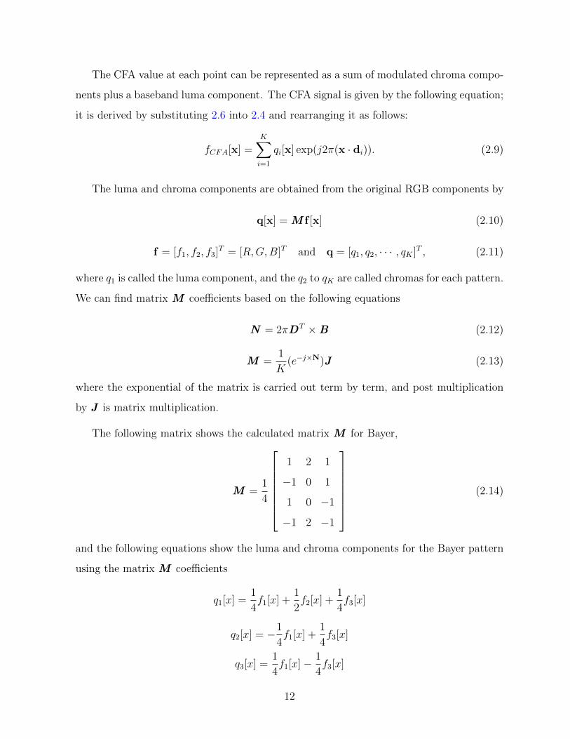
The CFA value at each point can be represented as a sum of modulated chroma compo-

nents plus a baseband luma component. The CFA signal is given by the following equation;

it is derived by substituting 2.6 into 2.4 and rearranging it as follows:

fCFA[x] =K∑i=1

qi[x] exp(j2π(x · di)). (2.9)

The luma and chroma components are obtained from the original RGB components by

q[x] = M f [x] (2.10)

f = [f1, f2, f3]T = [R,G,B]T and q = [q1, q2, · · · , qK ]T , (2.11)

where q1 is called the luma component, and the q2 to qK are called chromas for each pattern.

We can find matrix M coefficients based on the following equations

N = 2πDT ×B (2.12)

M =1

K(e−j×N)J (2.13)

where the exponential of the matrix is carried out term by term, and post multiplication

by J is matrix multiplication.

The following matrix shows the calculated matrix M for Bayer,

M =1

4

1 2 1

−1 0 1

1 0 −1

−1 2 −1

(2.14)

and the following equations show the luma and chroma components for the Bayer pattern

using the matrix M coefficients

q1[x] =1

4f1[x] +

1

2f2[x] +

1

4f3[x]

q2[x] = −1

4f1[x] +

1

4f3[x]

q3[x] =1

4f1[x]− 1

4f3[x]

12

q4[x] = −1

4f1[x] +

1

2f2[x]− 1

4f3[x]

. In the frequency domain, using the standard modulation property of the Fourier trans-

form, we find

FCFA(u) =K∑i=1

Qi(u− di) where Qi(u) , F{qi[x]}. (2.15)

Basic frequency-domain demosaicking involves extracting the chroma components with

bandpass filters separately, demodulating them to baseband and reconstructing the esti-

mated RGB signal based on these signals with

f [x] = M †q[x] (2.16)

where M † is the pseudo inverse matrix of M .

2.2 General methods for demosaicking

The earliest demosaicking techniques employ some well-known interpolation methods

like bilinear interpolation, cubic spline interpolation and nearest neighbor replication.

Later on, inter channel correlation has been used to reconstruct the red and blue col-

ors using red-to-green and blue-to-green ratio. In fact, these algorithm are based on the

assumption that the hue changes smoothly along neighboring pixels. In these methods

[8], the green component will be reconstructed using bilinear interpolation. Using the es-

timated green component, the red and blue color components will be reconstructed using

red-to-green and blue-to-green ratios. To be more precise, the interpolated red hue/ blue

hue value will be multiplied by the green value to determine the missing red/ blue value

at each pixel location. In some other works, the color difference is used instead of color

ratio [32]. These methods are not working well for high resolution data sets [30]. There

are some methods using wavelet transform, and some method applied frequency domain

based demosaicking algorithm.

13

2.2.1 Interpolation techniques

One of the simplest demosaicking methods is bilinear or bicubic interpolation. In

this method, the values of missing color components are estimated by interpolation of

neighboring pixel information. Figure 2.2 and 2.3 show a linear interpolation in Bayer

pattern.

Figure 2.2: Bilinear interpolation for green components for the Bayer pattern

G22 =1

4(G12 +G21 +G23 +G32) (2.17)

Figure 2.3: Bilinear interpolation for red/ blue components for the Bayer pattern

R22 =1

4(R11 +R13 +R31 +R33) (2.18)

R12 =1

2(R11 +R13) (2.19)

An interpolation based technique called Bayer reconstruction transforms RGB color

space to Y CrCb. The luminance image, Y , is reconstructed from green component after

14

applying bilinear interpolation on the green channel. The chroma values, Cr/Cb, for the

given red/blue components will be calculated by Cr = R − Y , and Cb = B − Y [14]. The

missing chroma will be estimated using bilinear interpolation. The results transform to

the RGB color space at the end.

2.2.2 Edge-directed interpolation

Some demosaicking techniques perform adaptive interpolation along the edges to create

better results. These methods use different edge classifiers like horizontal or vertical edge

classifiers, the gradients, the Laplacian operator and the Jacobian before green channel

interpolation. The interpolation applies to the selected direction afterward [1]. Some other

methods use a weighting scheme, and estimate the missing information using neighboring

pixels, and the calculated weights on the basis of the edge direction. Gunturk et al. [20]

also used the edge directed interpolation in their alternating projections algorithm. The

local homogeneity for each pixel has been measured in Hirakawa et al. [23]. They select the

interpolation direction using the homogeneity function in each pixel’s neighborhood. The

reconstructed images using edge-directed interpolation are usually sharper, and it contains

less blurring artifacts. Thus the results of demosaicked images using this method are good

in sharp regions, but they have poor results in problematic areas of the image [36].

2.2.3 Demosaicking methods using wavelet

In a typical wavelet-based demosaicking, first, the luminance image is formed using an

interpolation method. The red, green and blue components are also interpolated in the

same way. The wavelet transform will be applied on those interpolated images as well as

the luminance image separately, and four different wavelet coefficients will result. Some

merging scheme will be applied afterward, and the wavelet coefficient of each band of color

image will be modified by the wavelet coefficient of the luminance image.

Gunturk et al. [20] used a wavelet-based technique for demosaicking. They combine

the optimal edge directed interpolated image with the luminance image using wavelet

15

transform. Another wavelet based method presented in [14] improved the results visually

and quantitatively comparing to the bilinear and gradient-based interpolation methods. A

low complexity demosaicking algorithm using wavelet has been presented in [11].

Hirakawa et al. [24] presented a framework for demosaicking using the properties of

Smith-Barnwell filterbanks for demosaicking and denoising aspects. They present a gen-

eral framework for applying wavelet domain denoising algorithm as well as some existing

denoising algorithm prior to the demosaicking.

A hybrid demosaicking algorithm also has been presented in [27]. In this method,

they used the demosaicking algorithm presented in [29], and proposed an iterative post-

processing algorithm using wavelet decomposition to reduce the color artifacts around the

edges.

2.2.4 Demosaicking based on the frequency domain representa-

tion

The spatial multiplexing of red, green and blue color components can be represented in

the frequency domain with one luma component and several chroma components [3]. The

number of chromas usually depends on the number of samples in the pattern.

Demosaicking algorithms in the frequency domain usually involve extracting of luma

and modulated chromas using two dimensional filters. In the Bayer pattern, one luma

and three chromas will be extracted using passband filters, and the RGB values will be

estimated in each spatial location using luma and chroma components, as we explained in

section 2.1.

Since the components in the frequency domain representation are usually more isolated,

the image quality will improve compared to the spatial domain methods. Moreover, some

chromas with less interference with the luma can be used to reconstruct an image with less

aliasing effect. A method proposed in [21] used the high frequency information of the green

image to reconstruct and enhance the red and blue color information. Another method

presented in [16] designed an adaptive filter to extract the chromas with less overlap, and it

16

reduce the aliasing effect. LSLCD method [29] is one of the state of art algorithm that has

been described in frequency domain. This method optimized the filters and reduced the

overlap between luma and chroma components using least-square optimization method.

2.3 Image quality measurement

There are different metrics for image quality measurement. In this work, two metrics

will be calculated: peak signal-to-noise ratio (PSNR) and S-CIELAB. These two metrics

provide numerical comparison between the original image and the demosaicked image, and

help to compare different demosaicking algorithms.

2.3.1 Peak Signal-to-Noise Ratio

Mean-squared error and peak signal-to-noise ratio are two commonly used measures to

compare the reconstructed image with the original image. For an N1×N2 image RGB(i, j),

the MSE value for R, G and B will be calculated as follows:

MSE(R) =N1∑i=1

N2∑j=1

(R(i, j)−R(i, j)Reconstructed)2

N1 ×N2

(2.20)

MSE(G) =N1∑i=1

N2∑j=1

(G(i, j)−G(i, j)Reconstructed)2

N1 ×N2

(2.21)

MSE(B) =N1∑i=1

N2∑j=1

(B(i, j)−B(i, j)Reconstructed)2

N1 ×N2

(2.22)

CMSE =MSE(R) +MSE(G) +MSE(B)

3. (2.23)

The value of MSE, usually depends on the image intensity scaling. To solve this problem,

PSNR has been introduced, which measure the estimated error in decibels (db). Larger

values of PSNR shows better quality of reconstructed image. Since the values of pixels

in one image is scaled between [0 1], the following equation calculates the PSNR of an

image and its demosaicked image

CPSNR = 10 log10(1

CMSE) (2.24)

17

2.3.2 S-CIELAB

S-CIELAB is a metric based on L*a*b* color space, and it better measures perceptual

color difference. S-CIELAB gives us more accurate information about the image quality

viewed by human observer. The CIELAB metric is suitable for measuring color difference

of large uniform color targets. The S-CIELAB metric extends the CIELAB metric to color

images.

To measure perceptual difference between two lights using the CIELAB, the spectral

power distribution of the two lights are first converted to XYZ representations, which reflect

(within a linear transformation) the spectral power sensitivities of the three cones on the

human retina. The spatial filtering pre-processing step will be applied in an opponent color

space. The opponent color space contains one luminance and two chrominance channels

[26]. The following equation shows the linear transform between the XYZ color space to

opponent channel, AC1C2.A

C1

C2

=

0.297 0.72 −0.107

−0.449 0.29 −0.077

0.086 −0.59 0.501

X

Y

Z

(2.25)

The filtering step contains the two-dimensional separable convolution kernels. These ker-

nels are in the form of a series of Gaussian functions that can be found in [26]. Then,

the filtered opponent channels will be transformed back into XYZ space using the inverse

transform function. The XYZ values are transformed into an L*a*b* space, in which equal

distance is supposed to correspond to equal perceptual difference (perceptually uniform

space). Then, the perceptual difference between the two targets can be calculated by

taking the Euclidean distance of the two in this L*a*b* space. The S-CIELAB software

presented in [26] has been used in this research.

Color discrimination and appearance is a function of spatial pattern. In general, as the

spatial frequency of the target goes up (finer variations in space), color differences become

harder to see, especially differences along the blue-yellow color direction.

So, if we want to apply the CIE L*a*b* metric to color images, the spatial patterns of

the image have to be taken into account. The goal of the S-CIELAB metric is to add a

18

spatial pre-processing step to the standard CIELAB metric to account for the spatial-color

sensitivity of the human eye.

2.4 Review of different CFA patterns

Color Filter Arrays (CFAs) vary due to the type and placement of their color filters.

Each filter in a CFA is sensitive to a specific range of wavelengths to detect a certain

color. Most CFAs contain three primary color components: red, green and blue. Some of

them have an additional panchromatic/white filter as well. There are also some CFAs with

complementary color components: cyan, magenta and yellow. The basic CFA structure

containing four pixels is called Bayer, with two green, one blue and one red filter.

Due to the human eye sensitivity to the green light, usually the number of green filters

is twice as large as for the rest of the color components in RGB CFAs.

2.4.1 Three channel CFAs

The type of color filters in three channel CFAs can be either red, green and blue or

cyan, magenta and yellow. There are different types of structures with red, green and blue

filters like Bayer, Fujifilm [19] and Diagonal stripe pattern.

Bayer CFA pattern

Bayer is the three channel CFA, containing two green, one blue and one red in each

2× 2 pattern. It is used in many cameras like Canon, Olympus, Lumix and Sony. Due to

the popularity of Bayer pattern, many demosaicking methods have been designed for it.

Figure 2.4 shows one period of the Bayer pattern.

Fujifilm X-Trans pattern

The Fujifilm X-Trans pattern, as we can see in Figure 2.5 is a three channel 6×6 pattern.

It can be considered as a 3 × 6 pattern where half of the pattern is the shifted version of

19

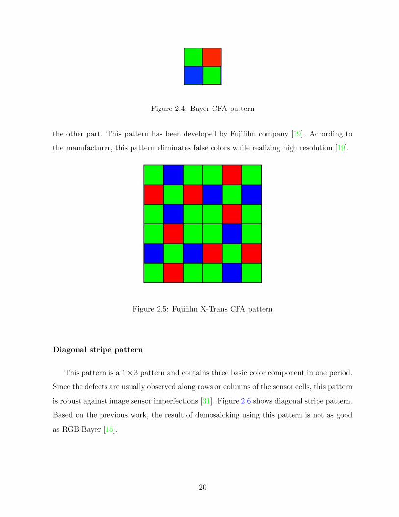
Figure 2.4: Bayer CFA pattern

the other part. This pattern has been developed by Fujifilm company [19]. According to

the manufacturer, this pattern eliminates false colors while realizing high resolution [19].

Figure 2.5: Fujifilm X-Trans CFA pattern

Diagonal stripe pattern

This pattern is a 1× 3 pattern and contains three basic color component in one period.

Since the defects are usually observed along rows or columns of the sensor cells, this pattern

is robust against image sensor imperfections [31]. Figure 2.6 shows diagonal stripe pattern.

Based on the previous work, the result of demosaicking using this pattern is not as good

as RGB-Bayer [15].

20

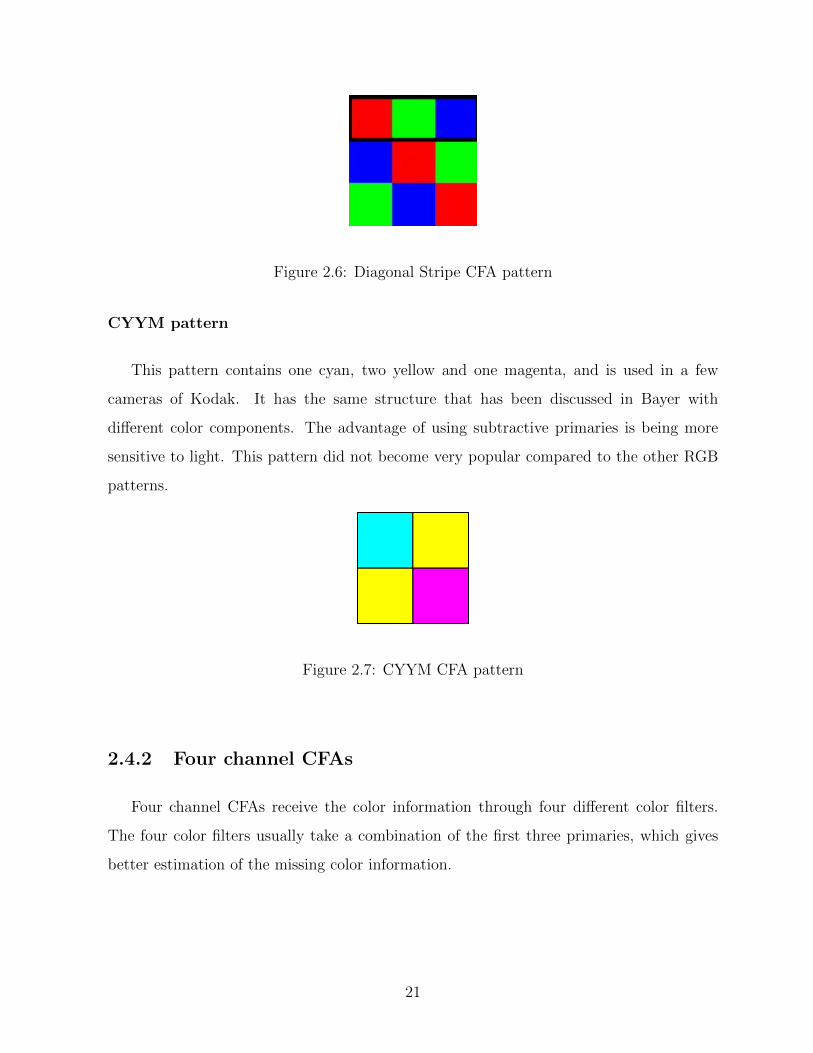
Figure 2.6: Diagonal Stripe CFA pattern

CYYM pattern

This pattern contains one cyan, two yellow and one magenta, and is used in a few

cameras of Kodak. It has the same structure that has been discussed in Bayer with

different color components. The advantage of using subtractive primaries is being more

sensitive to light. This pattern did not become very popular compared to the other RGB

patterns.

Figure 2.7: CYYM CFA pattern

2.4.2 Four channel CFAs

Four channel CFAs receive the color information through four different color filters.

The four color filters usually take a combination of the first three primaries, which gives

better estimation of the missing color information.

21

RGBE pattern

This is a Bayer-like pattern, where one of the green filters is modified to emerald, and

is used in a few Sony cameras. According to the manufacturer [42], using the emerald

filter reduces the color reproduction errors, and also records images closer to the human

eye perception.

Figure 2.8: RGBE CFA pattern

RGBW pattern

There are different kinds of RGBW patterns. The most simple pattern is RGBW-Bayer

which is a Bayer-like pattern. One of the green filters has been replaced with panchromatic/

white filter in this pattern. Another popular pattern is RGBW-Kodak CFA, and it has

been used in many cameras. This pattern is a 4 × 4 and half of the filters in the pattern

are white. There is also a 5× 5 pattern, that has been introduced in [45]. These patterns

will be studied in detail in Chapter 3 and 4.

Figure 2.9: RGBW-Bayer CFA pattern

22

CYGM pattern

Due to the human eye sensitivity to green color, a yellow color filter has been replaced

by a green filter in CYYM three channel pattern. Therefore, the pattern has one cyan,

one yellow, one green and one magenta to provide a compromise between maximum light

sensitivity and high color quality. It has been used in Nikon and Canon cameras such as

Powershot S10, Canon digital IXUS S100 for a period of time, but it has been replaced

with other patterns like Bayer very soon there after.

Figure 2.10: CYGM CFA pattern

2.5 Noise effect on CFA image

CFA sensors capture an image through the photo-electric conversion mechanism of a

silicon semiconductor. Incoming photons produce free electrons within the semiconductor

in proportion to the amount of incoming photons and those electrons are gathered within

the imaging chip. Image capture is therefore essentially a photon-counting process.

As such, image capture is governed by the Poisson distribution, which is defined with

a photon arrival rate variance equal to the mean photon arrival rate. The arrival rate

variance is a source of image noise because if a uniformly illuminated, uniform color patch

is captured with a perfect optical system and sensor, the resulting image will not be

uniform but rather have a dispersion about a mean value. The dispersion is called image

noise because it reduces the quality of an image when a human is observing it. Image noise

can also be structured, as is the case with dead pixels or optical pixel crosstalk. We focus

23

on the Poisson-distributed noise (also called shot noise) with the addition of electronic

amplifier read noise, which is modeled with a Gaussian distribution [2].

2.5.1 Demosaicking methods with a noise reduction stage

Many demosaicking algorithms have been designed for noise-free CFAs. Recently, the

effect of noise on the captured image has been addressed in some other works, and they

present demosaicking algorithms for noisy images. These methods mainly focus on restoring

more details and reducing the amount of noise in the reconstructed image. In demosaicking

methods with a noise reduction stage, usually, the noise will be modeled and added to the

input image for simulation. Jeon and Dubois modeled the noise in the white-balanced,

gamma corrected signal as signal independent white Gaussian noise. They used three

different variances for different color channels of RGB Bayer CFAs [18].

In some previous works, the noise reduction step is applied to the demosaicked image,

while some other methods implement the demosaicking stage after noise reduction. The

effect of noise in low-light images has been addressed in [7]. They applied denoising step

on the noisy image prior to the demosaicking step to prevent further corruption in the

demosaicking process. Their method results in sharper low-light images, and reduces noise

artifacts in the demosaicking step.

Most of the recent works in this area apply joint denoising and demosaicking schemes to

the noisy image. Nawrath et al.[35] present a non-local filtering for the denoising step and

produce demosaicked image with less color artifacts and less blurry effect. They stated that

the difference between two color channels is locally nearly constant. According to this rule,

they applied a non-local means filter to the joined difference channels and interpolated color

image. The state of the art joint demosaicking and denoising method for RGB-Bayer CFA

has been proposed in [25]. As we discussed before, the panchromatic/white filter receives

more light comparing to the other color filters. Due to the lack of literature on joint

demosaicking and denoising algorithm using RGBW CFAs, we propose both demosaicking

algorithm and noise reduction method for RGBW patterns.

There are several methods to reduce noise in gray scale or color images, but they are not

24

working well for CFA images. Sung Hee et al. [43] proposed a noise reduction method for

CFA images. In this method, the denoising step will be applied before demosaicking to the

input CFA image. They also presented a comparison between two adaptive demosaicking

algorithm (Hirakawa and Dubois) and a bilinear demosaicking method. They compare the

demosaicking error as a function of noise-level for the mentioned methods. They stated that

the adaptive algorithm performs extremely well under low sensor noise conditions, their

performance decreases as noise increases compared to the bilinear method. Consequently,

there is an interaction between input noise and the demosaicking algorithm that is used.

In some joint denoising-demosaicking algorithm, we need to estimate the noise value

on a specific image before applying the noise reduction step. An accurate noise estimator

would significantly benefit many image denoising methods. There are some noise estimation

method designed for images. A recent work presented a method to estimate additive noise

by utilizing the mean deviation of a smooth region selected from a noisy image. The noise

distribution is estimated by computing the average mean deviation of all non-overlapping

blocks in the smooth region [41].

Tomasi et al.[44] presented the bilateral filter. This method is based on matching

distance (spatial), and similarity (intensity) criteria, and preserve sharp edges in noise

reduction process.

Non-local filter method presented by Buades et al. [5], finds the similar patches to the

area around each pixel, in entire image, and weights the similar patches by their similarity.

Each pixel will be replaced by the weighted average of the center pixels of the matching

patch. This method is slow in practice, and it usually searches for similar patches in a

small area around each pixel.

Later on, Dabov et al. [12] presented BM3D method similar to Buades’s method.

In this method similar patches will be collaboratively filtered to provide an estimate for

each pixel in the blocks. So, there will be several estimates for each pixel, and this method

combined them to generate basic estimate of the true image. Then, another block matching

step will be performed on the basic estimate, as a final denoising step.

The BM3D method, is based on an enhanced sparse representation in the transform

25

domain, and it consist of two main steps: grouping and aggregation. The enhancement of

the sparsity is achieved by grouping similar 2D image blocks into 3D data arrays which is

known as grouping step. The collaborative filtering is applied on these 3D blocks afterward.

This step contains three parts: 3D transformation of a group, shrinkage of the transform

spectrum, and inverse 3D transform. The filtered blocks will returned to their original

positions. Because of the overlapping of the blocks, there will be different estimates for

each pixel. During aggregation step, those redundant information will be combined using

averaging procedure.

Another method called clustering-based sparse representation (CSR) have been pro-

posed in 2011. In this method, a dictionary of reference patches will be created, and the

patches will be built as weighted combination of these dictionary patches. The average

value of all patches in the same location will be assigned as pixel value[13].

According to a comparison has been presented in [6] a different denoising method,

BM3D is working well among the listed method, and it preserve details of the image as

well as sharp edges.

2.5.2 State of art joint demosaicking-denoising method for noisy

RGB-Bayer patterns

Jeon and Dubois proposed a state of art demosaicking-denoising method for RGB-Bayer

pattern. They used the least-square demosaicking method that has been proposed in [18].

For the design, they artificially add noise with different noise levels to the input images,

and use the noisy images for training a set of the least-square filters. Several least-square

filters adapted to different noise level have been designed in this method. They estimate the

noise level of the input using Amer et al. noise estimation method [4], and an appropriate

set of filters will be chosen using the estimated parameters.

Since the reconstruction of luma components is crucial in the demosaicking systems,

and results in better quality of the reconstructed image, they utilize a separate noise reduc-

tion stage for luma components. They used the Block Matching 3D (BM3D) denoising

26

algorithm [12] , which is one of the state of art denoising methods. The luma denoising

step improves the quality of output RGB image.

2.6 Summary

In this chapter, we reviewed different demosaicking algorithms in the space domain

and the frequency domain. Also, different CFA patterns have been studied in this chapter.

There is not enough literature on some of the discussed CFAs, and they need to be studied

in detail. Some commercially well-known CFAs will be studied in this work, and the

demosaicking algorithm will be provided for these CFAs. Four-channel CFAs are widely

used in cameras recently. The effect of noise on four-channel CFAs with panchromatic

filters has not been fully studied. The frequency domain analysis containing noise reduction

algorithm using RGBW CFAs will be discussed in this research.

27

Chapter 3

Demosaicking algorithms in the

noise-free case

As discussed in the previous chapter, there are many popular CFAs, and some related

demosaicking algorithms have been provided in the literature in each case. In this thesis we

narrow down our research to two main categories: three-channel CFAs, and four channel

CFAs, since these cover most cases in actual use. We start by considering the noise-free

(or low-noise) case. Due to the lack of published research on the Fujifilm X-Trans pattern

and given its claimed advantages, we focused on this pattern as a sample of three-channel

CFAs.

The RGBW CFAs have been chosen as four-channel CFAs, due to their anticipated

benefits in the noisy case, and three different RGBW patterns have been analyzed in our

work. The results of the reconstructed images have been compared, and the best RGBW

pattern has been chosen for the noise reduction step. The following sections explain the

details of the demosaicking algorithms for different identified patterns.

3.1 Demosaicking algorithm structure

Different CFA patterns may have different sizes. Using the smallest repeated pattern,

the CFA signal is sampled on lattice Λ = Z2 with reciprocal lattice Λ∗ = Z2.

28

Using these lattices, we can model the CFA signal as a sum of luma and chroma

components.

fCFA[x] =K∑i=1

qi[x] exp(j2π(x · di)), where

We also calculate matrix B and matrix D for this CFA pattern, as described in chapter

2. Matrix M also will be calculated afterward.

Since we have three individual color components for three-channel CFAs in the space

domain related to R, G and B, there should be at least three individual components in

the frequency domain (chromas) as well. Generally, there are C filter types, where C = 3

for three-channel CFAs, and C = 4 for four-channel CFAs, and there should be at least

K = C components for a sample CFA.

Using Fourier analysis (discrete-domain Fourier series), we find that the spatial mul-

tiplexing of C components is equivalent to the frequency domain multiplexing of K com-

ponents. The basic demosaicking algorithm involves extracting the K components using

bandpass filters, demodulating them to baseband and reconstructing the C original com-

ponents. This has no advantage over spatial interpolation. However, we can reduce the

number of K components, and design an adaptive algorithm.

Although the number of chromas vary depending on the CFA pattern in different cam-

eras, there should be some relation between chromas. It is always beneficial to decrease

redundancy between chromas to three basic components, since it reduces the computa-

tional complexity. The smaller number of chromas also results in less overlap between

chromas. It will also lead us to more accurate chroma extraction.

Using matrix M , we can find the dependency of chromas. We can divide chromas into

several groups of dependent chromas. We have to choose one chroma per group as a basic

chroma, and fully extract it. Then we will be able to fully reconstruct the rest of chromas

in the same group. The group assignment of chromas are not necessarily unique, and there

should be a minimum of three basic chromas for each three-channel pattern and four for

four-channel CFAs.

29

In this section, we present our applied demosaicking algorithm as a general model, so

it can be applied on any other CFA pattern. As we discussed in the previous section, the

following equation shows the relation between chroma components in frequency domain

and the RGB image.

q [x] = Mf [x] (3.1)

f =[f1, f2, f3, f4

]T(3.2)

q =[q1, q2, ... , qK

]T(3.3)

Assuming M is a K × C matrix, we are concerned with the case where K > C, and

we would like to simplify matrix M .

We can minimize the number of rows in M and decrease the number of color compo-

nents in the frequency domain as follows in two steps. First, we delete zero rows of M as

not relevant. Second, as experience shows that in most cases of interest, the rows of M

each belong to one of C one-dimensional sub-spaces of RC , we need to find those rows in

matrix M .

Since we simplify the matrix M , we will be able to design the adaptive demosaicking

algorithm. In the adaptive algorithm, only one color component in each group will be

estimated, and it will be used to determine all the others belonging to the same group.

The specific component in each group can be chosen locally based on an estimate of which

component in its group is least affected locally by crosstalk. Once all chromas are adap-

tively estimated, they can be remodulated and subtracted from the CFA signal to estimate

the luma.

The following examples show the process of matrix M simplification more clearly for

different CFAs. In the case of Bayer, as we discussed in Section 2.1, equation 2.13 we have

M =1

4×

1 2 1

−1 0 1

1 0 −1

−1 2 −1

. (3.4)

30

In this CFA m3i = −m2i, and thus q3 = −q2. Thus, only one of q2 and q3 is needed to

reconstruct F , and the best one can be chosen locally using an adaptive algorithm.

A more complex case is the Fujifilm X-Trans CFA, where K is 18. This will be studied

in detail in Section 3.2. Five rows of M are zero, so they can be ignored. There are

thirteen remaining rows, and we call the downsized matrix M’ .

M’ =1

9×

2 5 2

−0.25− 0.43j 0.5 + 0.86j −0.25− 0.43j

−0.25 + 0.43j 0.5− 0.86j −0.25 + 0.43j

0.5− 0.86j −1 + 1.73j 0.5− 0.86j

0.5 + 0.86j −1− 1.73j 0.5 + 0.86j

−0.25 + 0.43j 0.5− 0.86j −0.25 + 0.43j

−0.25− 0.43j 0.5 + 0.86j −0.25− 0.43j

−1 2 −1

−1 2 −1

0.75 + 1.3j 0 −0.75− 1.3j

−0.75− 1.3j 0 0.75 + 1.3j

0.75− 1.3j 0 −0.75 + 1.3j

−0.75 + 1.3j 0 0.75− 1.3j

(3.5)

These rows lie in three 1D subspaces spanned by a1[2, 5, 2], a2[−1, 2, 1] and a3[1, 0,−1]

where a1, a2 and a3 are arbitrary complex constants which we can choose according to our

convenience.

Next consider Kodak RGBW. In this CFA C = 4 and K = 16, but four rows are zero,

31

and can be ignored. The remaining rows are:

M ’ =1

16×

2 4 2 8

−1 + j 0 1− j 0

−1− j 0 1 + j 0

1− j 0 −1 + j 0

1 + j 0 −1− j 0

2 −4 2 0

−2 4 −2 0

−1 + j 0 1− j 0

1− j 0 −1 + j 0

−1− j 0 1 + j 0

1 + j 0 −1− j 0

−2 −4 −2 8

(3.6)

By looking at matrix M’ , there are some obvious similarities between rows. They lie

in four 1D subspaces spanned by a1[1, 2, 1, 4] as group one, a2[1, 0,−1, 0] as group two,

a3[1,−2, 1, 0] as group three and a4[1, 2, 1,−4] as group four. These subspaces can be

easily found by inspection.

If we can reconstruct one chroma based on the other, we assume those chromas belong

to the same class. Here we assume Luma (first row) as a separate class, rows 2 − 5 and

8− 11 as second class, rows 6 and 7 as our third class, and the last row as the fourth class

of chromas.

The matrix J is defining the four input channels: R, G, B and W, while each column

of the matrix represents one of the colors in this pattern. Panchromatic pixels in the CFA

will be calculated using equation 3.7.

W = aR(R) + aB(B) + aG(G) (3.7)

In the frequency domain, the Fourier transform of the CFA signal is

FCFA(u) =N∑i=1

Qi(u− di) where Qi(u) , F{qi[x]}. (3.8)

32

The chroma components are extracted with bandpass filters centered at the frequencies di.

The next step in the demosaicking algorithm is reconstructing the full RGB color image

using the pseudo inverse matrix M †.

There are two main issues in adaptive algorithm: how to design appropriate filters

to extract the modulated chroma components, and how to adaptively estimate the basic

chroma in each group to minimize the effect of crosstalk. These issues will be addressed

for each of the CFA patterns to be presented in the subsequent section.

3.2 Three channel color filter array

The three-channel color filter arrays usually contain three primary color filters: red,

green and blue. Due to the different CFA structures, the number of each color filter type

in one period of the pattern varies. The most widely used three-channel CFA is Bayer,

containing two green, one blue and one red filter in one period of the pattern. Because

of the human eye’s sensitivity to the green color, the number of green pixels in most of

the three channel CFAs is usually twice or almost twice the number of blue or red pixels.

The quality of the output images depends on the number of different color filters in each

pattern as well as the arrangement of the color filters in the template.

3.3 Demosaicking for the Fujifilm X-Trans pattern

In this work, we implement demosaicking algorithms related to the Fujifilm X-Trans

CFA pattern. The Fujifilm CFA pattern is a 6× 6 template containing 20 green pixels, 8

blue and 8 red as we can see in Figure 3.1. The number of green pixels is more than the

total number of blue and red pixels. This template provides a higher degree of randomness

with an array of 6×6 pixel units. According to the manufacturer, without using an optical

low-pass filter, moire and false colors are eliminated while realizing high resolution [19].

Analysis of this pattern is more complicated than for the Bayer pattern due to the large

number of sensors in one period of the CFA. In the following sections, two different analysis

33

approaches will be presented for Fujifilm X-Trans pattern.

Figure 3.1: Fujifilm X-Trans CFA pattern

Demosaicking algorithm

Although the pattern is generally viewed as 6 × 6, it is in fact 3 × 6 with periodicity

given by a hexagonal lattice. The second 3× 6 part can be assumed as a shifted version of

the first half. The CFA signal is sampled on lattice Λ = Z2 with reciprocal lattice Λ∗ = Z2.

A lattice and it’s corresponding reciprocal lattice to represent the periodicity of the CFA

pattern can be given by

∨Γ =

6 3

0 3

, ∨Γ∗ =

16

0

−13

13

. (3.9)

The analysis of this CFA can be carried out using the general theory described in

[18], and summarized in Chapter 2. According to the analysis, the CFA signal can be

represented as a sum of modulated chroma components plus a baseband luma component.

34

The CFA signal is given by

fCFA[x] =K∑i=1

qi[x] exp(j2π(x · d i)) where K = 18. (3.10)

According to [18], d i refers to the columns of matrix D and they are coset represen-

tatives of Λ∗ in Γ∗. The matrix D is a 2 ×K matrix where K is the number of samples

in one period of the lattice, which is equal to 18 for the Fujifilm pattern. The following

matrix is used here

D =1

6×

0 2 −2 1 −1 2 −2 1 −1 0 0 2 −2 3 −1 3 1 3

0 0 0 1 −1 2 −2 −1 1 −2 2 −2 2 −1 3 1 3 3

.(3.11)

The luma and chroma components are obtained from the original RGB components by

q [x] = M f [x] (3.12)

f = [f1, f2, f3]T = [R,G,B]T and q = [q1, q2, · · · , q18]T . (3.13)

For finding matrix M we need to calculate matrices B and J . Also, b i refers to the

columns of matrix B which gives the coset representatives of Γ in Λ. We use

B =

0 1 2 0 1 2 0 1 2 0 1 2 0 1 2 0 1 2

0 0 0 1 1 1 2 2 2 3 3 3 4 4 4 5 5 5

. (3.14)

Color channels will be represented by

J =

0 0 0 1 0 1 0 0 0 0 1 0 0 0 0 0 1 0

1 0 1 0 1 0 1 0 1 1 0 1 0 1 0 1 0 1

0 1 0 0 0 0 0 1 0 0 0 0 1 0 1 0 0 0

T

. (3.15)

The following matrix shows the calculated matrix M for 18 components using 2.13 in

35

Section 2.1. Note that only 13 components are nonzero.

M =

0.2222 0.5556 0.2222

−0.0278− 0.0481j 0.0556 + 0.0962j −0.0278− 0.0481j

−0.0278 + 0.0481j 0.0556− 0.0962j −0.0278 + 0.0481j

0 0 0

0 0 0

0.0556− 0.0962j −0.1111 + 0.1925j 0.0556− 0.0962j

0.0556 + 0.0962j −0.1111− 0.1925j 0.0556 + 0.0962j

0 0 0

0 0 0

−0.0278 + 0.0481j 0.0556− 0.0962j −0.0278 + 0.0481j

−0.0278− 0.0481j 0.0556 + 0.0962j −0.0278− 0.0481j

−0.1111 0.2222 −0.1111

−0.1111 0.2222 −0.1111

0.0833 + 0.1443j 0 −0.0833− 0.1443j

−0.0833− 0.1443j 0 0.0833 + 0.1443j

0.0833− 0.1443j 0 −0.0833 + 0.1443j

−0.0833 + 0.1443j 0 0.0833− 0.1443j

0 0 0

(3.16)

In the frequency domain, using the standard modulation property of the Fourier trans-

form, we find

FCFA(u) =18∑i=1

Qi(u− d i) where Qi(u) , F{qi[x]} (3.17)

Figure 3.2 shows the power spectral density of a sample X-Trans CFA image, illustrating

the position of luma and chroma components in one unit cell of Λ∗.

Basic frequency-domain demosaicking involves extracting the luma and the twelve

nonzero chroma components with bandpass filters separately, demodulating them to base-

band and reconstructing the estimated RGB signal based on these signals with

f [x] = M †q[x] (3.18)

36

Figure 3.2: Luma- Chroma position for Fujifilm X-Trans pattern

where M † is the pseudo inverse matrix of M .

Due to the similarity of different chromas and their distance from luma in this pattern,

three baseband Gaussian filters have been designed in our basic implementation. The

Gaussian filters are 2D filter with σ = 2.32 for both dimension. The filter sizes have been

set experimentally. Different chromas have been filtered by modulating these Gaussian

filters to the different band center frequencies. The first filter extracted q2, q3, q10 and q11.

The second one has been used for q6, q7, q12 and q13 and the last one extracts q14, q15, q16

and q17.

The Luma component will be extracted as follows:

q1[x] = fCFA[x]−18∑i=2

qi exp(j2π(x · d i)). (3.19)

Although we model the whole system for 18 components, there are 5 components with

qi[x] equal to zero. These are correspond to d4, d5, d8, d9 and d18.

Based on the dependence of different chroma components we can categorize all 18

component into 5 groups and estimate the rest of the components based on them. The

37

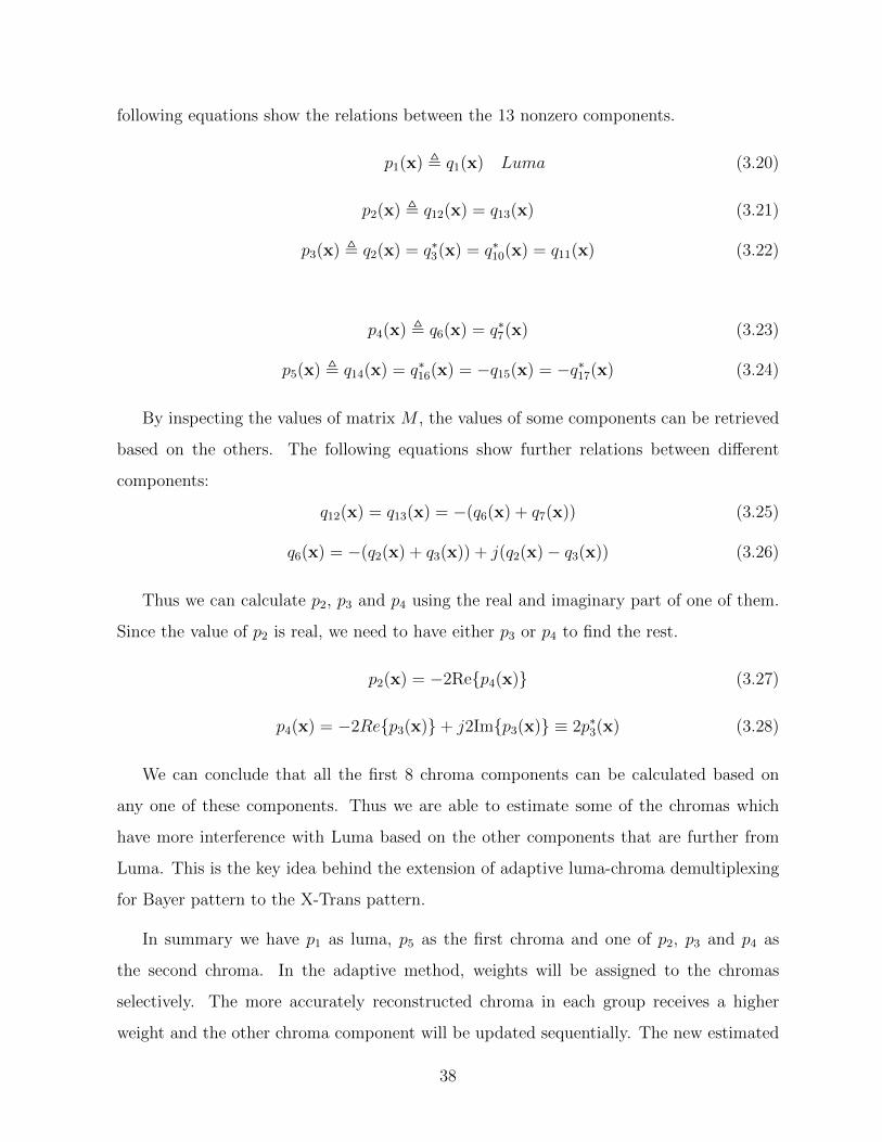
following equations show the relations between the 13 nonzero components.

p1(x) , q1(x) Luma (3.20)

p2(x) , q12(x) = q13(x) (3.21)

p3(x) , q2(x) = q∗3(x) = q∗10(x) = q11(x) (3.22)

p4(x) , q6(x) = q∗7(x) (3.23)

p5(x) , q14(x) = q∗16(x) = −q15(x) = −q∗17(x) (3.24)

By inspecting the values of matrix M , the values of some components can be retrieved

based on the others. The following equations show further relations between different

components:

q12(x) = q13(x) = −(q6(x) + q7(x)) (3.25)

q6(x) = −(q2(x) + q3(x)) + j(q2(x)− q3(x)) (3.26)

Thus we can calculate p2, p3 and p4 using the real and imaginary part of one of them.

Since the value of p2 is real, we need to have either p3 or p4 to find the rest.

p2(x) = −2Re{p4(x)} (3.27)

p4(x) = −2Re{p3(x)}+ j2Im{p3(x)} ≡ 2p∗3(x) (3.28)

We can conclude that all the first 8 chroma components can be calculated based on

any one of these components. Thus we are able to estimate some of the chromas which

have more interference with Luma based on the other components that are further from

Luma. This is the key idea behind the extension of adaptive luma-chroma demultiplexing

for Bayer pattern to the X-Trans pattern.

In summary we have p1 as luma, p5 as the first chroma and one of p2, p3 and p4 as

the second chroma. In the adaptive method, weights will be assigned to the chromas

selectively. The more accurately reconstructed chroma in each group receives a higher

weight and the other chroma component will be updated sequentially. The new estimated

38

Figure 3.3: Fujifilm adaptive demosaicking system

chromas improve the luma estimation when using equation 3.19. Figure 3.3 shows the

structure of the adaptive demosaicking algorithm.

There are four chroma components which are very close to the luma: q2, q3, q10 and

q11. We are trying to find a more accurate value for q2, and calculate the other three

components using the updated q2. Since q2, q3, q6, q7, q10, q11, q12 and q13 are closer to the

luma, we used a weighted form of each one adaptively to reconstruct the q2 component

with least overlap with luma. In this method, the energy function has been calculated

between luma and one of each pairs of chromas. Every two symmetrically located chromas

have been assumed as a pair: q2 and q3, q6 and q7, q10 and q11, q12 and q13.

To optimize the weight assignment process, we create a filter to extract the overlapped

information in the middle of the Euclidean distance of luma and the given chroma. The

filtered information shows the average local energy as an overlapping index at that location.

39

Specifically, a baseband Gaussian filter hG, with a certain standard deviation rG has been

designed for this process. The rG has been set experimentally to give the best filtering

performance. The Gaussian filter has been modulated to the certain frequency between

luma and chroma, to filter the local energy. The modulated filter is shown as hGx. The

filtered signal will be squared and will be filtered using a 5 × 5 moving average filter

afterward.

This value has an inverse relation with the accuracy of the filtered chroma. So, we

assign the inverse form of energy index to the mentioned chroma as weight (w). Four

different weights have been calculated in this way, and each weight has been assigned to a

pair of above chromas. Therefore, the chroma having less overlap with the luma receives

more weight, and the least accurate one receives less weight in each pixel of the image.

Each of those four weights has been divided by the sum of w1 to w4 to make sure that

the total value of the assigned weights is equal to one. The following equations show the

weighting process.

energy = (fCFA ∗ hGx)2 ∗ h5×5 (3.29)

w =1

energy(3.30)

q2(x) =(w2)q2(x) + (w6)q6(x) + (w10)q10(x) + (w12)q12(x)

w2 + w6 + w10 + w12

(3.31)

q3(x) = q∗2(x) (3.32)

q10(x) = q∗2(x) (3.33)

q11(x) = q2(x) (3.34)

The updated q2 will be used to reconstruct the enhanced q3, q10, q11 and luma in

adaptive demosaicking algorithm. The luma component will also be updated afterward.

The non-adaptive algorithm extracts the chromas using the Gaussian filters and simply

reconstructs the RGB image using the extracted chromas.

In comparing demosaicking algorithms using Fujifilm and Bayer patterns, we note that

there were also three selected independent components in Bayer. Since the updated q2 in

40

the presented algorithm depend on q6, q10, q12 chromas, we will not be able to optimize

the weighting scheme that has been described above. Thus, we need to minimize the

dependency between chromas. The following method expresses the Bayer-like analysis for

the X-Trans Fujifilm pattern. In this method q2 will be reconstructed using two chromas,

and the assigned weights will be optimized.

Bayer-like analysis for Fujifilm CFA pattern

In this method we are trying to reconstruct the remaining thirteen components using

one luma and two chromas as we have before for Bayer. Since we are reconstructing an

RGB image, we need in fact three degrees of freedom. The signal q1 is a luma signal, given

by

q1[x] =1

9(2fR[x] + 5fG[x] + 2fB[x]) , fL[x] (3.35)

Note that this is different than the luma component in the Bayer CFA. There are essentially

two distinct chroma signals, which can be taken to be the same ones as in the Bayer CFA:

fC1[x] =1

4(−fR[x] + 2fG[x]− fB[x]) (3.36)

fC2[x] =1

4(−fR[x] + fB[x]) (3.37)

41

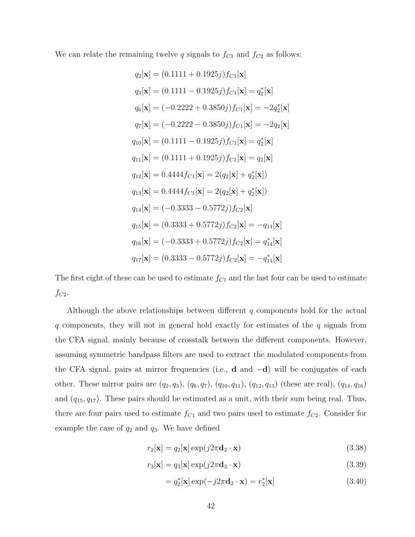
We can relate the remaining twelve q signals to fC1 and fC2 as follows:

q2[x] = (0.1111 + 0.1925j)fC1[x]

q3[x] = (0.1111− 0.1925j)fC1[x] = q∗2[x]

q6[x] = (−0.2222 + 0.3850j)fC1[x] = −2q∗2[x]

q7[x] = (−0.2222− 0.3850j)fC1[x] = −2q2[x]

q10[x] = (0.1111− 0.1925j)fC1[x] = q∗2[x]

q11[x] = (0.1111 + 0.1925j)fC1[x] = q2[x]

q12[x] = 0.4444fC1[x] = 2(q2[x] + q∗2[x])

q13[x] = 0.4444fC1[x] = 2(q2[x] + q∗2[x])

q14[x] = (−0.3333− 0.5772j)fC2[x]

q15[x] = (0.3333 + 0.5772j)fC2[x] = −q14[x]

q16[x] = (−0.3333 + 0.5772j)fC2[x] = q∗14[x]

q17[x] = (0.3333− 0.5772j)fC2[x] = −q∗14[x]

The first eight of these can be used to estimate fC1 and the last four can be used to estimate

fC2.

Although the above relationships between different q components hold for the actual

q components, they will not in general hold exactly for estimates of the q signals from

the CFA signal, mainly because of crosstalk between the different components. However,

assuming symmetric bandpass filters are used to extract the modulated components from

the CFA signal, pairs at mirror frequencies (i.e., d and −d) will be conjugates of each

other. These mirror pairs are (q2, q3), (q6, q7), (q10, q11), (q12, q13) (these are real), (q14, q16)

and (q15, q17). These pairs should be estimated as a unit, with their sum being real. Thus,

there are four pairs used to estimate fC1 and two pairs used to estimate fC2. Consider for

example the case of q2 and q3. We have defined

r2[x] = q2[x] exp(j2πd2 · x) (3.38)

r3[x] = q3[x] exp(j2πd3 · x) (3.39)

= q∗2[x] exp(−j2πd2 · x) = r∗2[x] (3.40)

42

Assuming we use mirror symmetric bandpass filters to estimate r2 and r3, we will necessarily

find

r3[x] = r∗2[x].

After demodulating these two signals to baseband, we find

q2[x] = r2[x] exp(−j2πd2 · x) (3.41)

q3[x] = r3[x] exp(−j2πd3 · x) (3.42)

= r∗2[x] exp(j2πd2 · x) = q∗2[x] (3.43)

Then, s2,3[x] , q2[x] + q3[x] is real, and can be used as an estimate of q2[x] + q3[x] =

0.2222fC1[x]. In a similar fashion: s10,11[x] , q10[x] + q11[x] is real, and can be used as an

estimate of q10[x] + q11[x] = 0.2222fC1[x]; s6,7[x] , q6[x] + q7[x] is real, and can be used as

an estimate of q6[x] + q7[x] = −0.4444fC1[x]; and finally, s12,13[x] , q12[x] + q13[x] is real,

and can be used as an estimate of q12[x] + q13[x] = 0.8888fC1[x].

We could combine these to form a non-adaptive estimate of fC1 by giving them equal

weighting:

fC1[x] = 0.250.2222

s2,3[x] + 0.250.2222

s10,11[x]− 0.250.4444

s6,7[x] + 0.250.8888

s12,13[x] (3.44)

= 98s2,3[x] + 9

8s10,11[x]− 9

16s6,7[x] + 9

32s12,13[x] (3.45)

or alternatively (and better, since in general s2,3 and s10,11 suffer more crosstalk than s6,7

and s12,13)

fC1[x] = −98s6,7[x] + 9

16s12,13[x]. (3.46)

A general formula is

fC1[x] = 92was2,3[x] + 9

2wbs10,11[x]− 9

4wcs6,7[x] + 9

8wds12,13[x] (3.47)

where wa + wb + wc + wd = 1.

A similar approach can be used to estimate fC2. We define s14,16[x] = q14[x] + q16[x]

to estimate q14[x] + q16[x] = −0.6666fC2[x] =, and s15,17[x] = q15[x] + q17[x] to estimate

q15[x] + q17[x] = 0.6666fC2[x] = Averaging these two,

fC2[x] = −34s14,16[x] + 3

4s15,17[x]. (3.48)

43

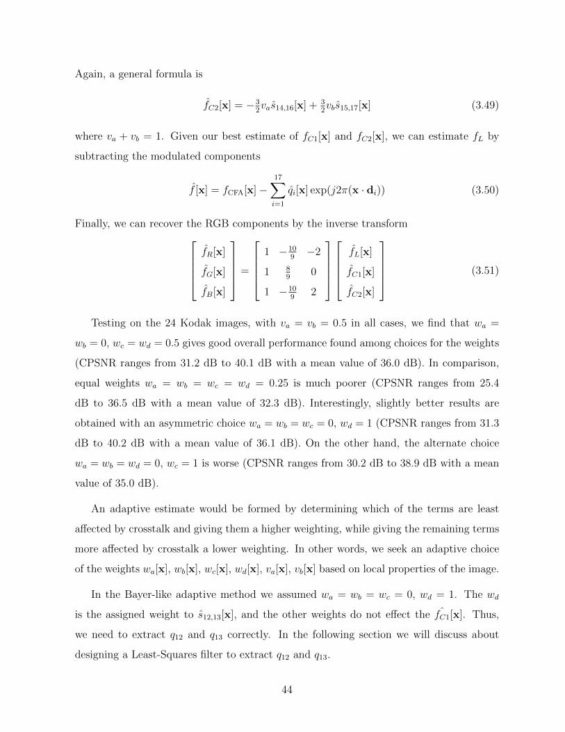
Again, a general formula is

fC2[x] = −32vas14,16[x] + 3

2vbs15,17[x] (3.49)

where va + vb = 1. Given our best estimate of fC1[x] and fC2[x], we can estimate fL by

subtracting the modulated components

f [x] = fCFA[x]−17∑i=1

qi[x] exp(j2π(x · di)) (3.50)

Finally, we can recover the RGB components by the inverse transformfR[x]

fG[x]

fB[x]

=

1 −10

9−2

1 89

0

1 −109

2

fL[x]

fC1[x]

fC2[x]

(3.51)

Testing on the 24 Kodak images, with va = vb = 0.5 in all cases, we find that wa =

wb = 0, wc = wd = 0.5 gives good overall performance found among choices for the weights

(CPSNR ranges from 31.2 dB to 40.1 dB with a mean value of 36.0 dB). In comparison,

equal weights wa = wb = wc = wd = 0.25 is much poorer (CPSNR ranges from 25.4

dB to 36.5 dB with a mean value of 32.3 dB). Interestingly, slightly better results are

obtained with an asymmetric choice wa = wb = wc = 0, wd = 1 (CPSNR ranges from 31.3

dB to 40.2 dB with a mean value of 36.1 dB). On the other hand, the alternate choice

wa = wb = wd = 0, wc = 1 is worse (CPSNR ranges from 30.2 dB to 38.9 dB with a mean

value of 35.0 dB).

An adaptive estimate would be formed by determining which of the terms are least

affected by crosstalk and giving them a higher weighting, while giving the remaining terms

more affected by crosstalk a lower weighting. In other words, we seek an adaptive choice

of the weights wa[x], wb[x], wc[x], wd[x], va[x], vb[x] based on local properties of the image.

In the Bayer-like adaptive method we assumed wa = wb = wc = 0, wd = 1. The wd

is the assigned weight to s12,13[x], and the other weights do not effect the ˆfC1[x]. Thus,

we need to extract q12 and q13 correctly. In the following section we will discuss about

designing a Least-Squares filter to extract q12 and q13.

44

Designing filter using Least-Square method

In the previous sections, we designed Gaussian filters for q2 and q10 which are close to

the luma. In this section, the least-squares method will be explained. We want to design

a filter to extract q12 and q13, or s12,13 = q12 + q13, which are all real. Let us first design

the complex filter to estimate q12, and it will be the same procedure for any other chroma.

We can call the design filter h12 for q12. We have:

r12[x] = (fCFA ∗ h12)[x] (3.52)

q12[x] = r12[x] exp(−j2πd12 · x) (3.53)

On the training image q12[x] = 0.4444fC1[x], r12[x] = q12[x] exp(j2πd12 · x). Let W (i) be

the support of the ith training image, i = 1, ..., P . Then the least-square filter is

h12 = arg minh

P∑i=1

∑x∈W (i)

∣∣∣(r(i)12 − h ∗ f

(i)CFA)[x]

∣∣∣2 (3.54)

Let S be the region of support of h12, |S| = NB, then

(h ∗ f (i)CFA)[n1, n2] =

∑(k1,k2)∈S

h[k1, k2]f(i)CFA[n1 − k1, n2 − k2] (3.55)

We prefer to express it in matrix form as follows. First, arrange the filter coefficients into

an NB×1 column matrix, taking the coefficients of h column by column from left to right.

h1D =

h(:, 1)

h(:, 2)...

h(:, Nfilt)

(3.56)

where NB = N2filt Let Nw =

∣∣W (i)∣∣, assumed the same for all i. Arrange r

(i)12 into an NB×1

column matrix in the same way.

r(i)1D,12 =

r

(i)12 (:, 1)

r(i)12 (:, 2)

...

r(i)12 (:, NW )

(3.57)

45

Then

r1D,12 = Z(i)h1D (3.58)

where Z(i) is an NW ×NB matrix. Each column of Z(i) is a reshaped version of f(i)CFA[n1−

k1, n2 − k2] for some k1 and k2, rearranged in the order of h1D.

Z(i)(:,m[k1, k2]) =

f

(i)CFA[n1 − k1, n2 − k2](:, 1)

f(i)CFA[n1 − k1, n2 − k2](:, 2)

...

f(i)CFA[n1 − k1, n2 − k2](:, NW )

(3.59)

where h1D[m[k1, k2]] = h[k1, k2].

Z is real value and r is complex. Equation 3.54 can be written in matrix form as

h12 = arg minh

P∑i=1

∣∣∣∣Z(i)h− r12(i)∣∣∣∣2 (3.60)

This is a standard least-squares problem with solution [34]

h1D,12 = [

p∑i=1

Z(i)TZ(i)]−1[

p∑i=1

Z(i)T r(i)1D,12] (3.61)

h12 =

h12(1, 1) · · · h12(Nfilt, 1)

.... . .

...

h12(1, Nfilt) · · · h12(Nfilt, Nfilt)

(3.62)

Results and discussion

The proposed demosaicking algorithms for the Fujifilm X-Trans pattern have been im-

plemented in the Matlab environment. We reconstruct 24 Kodak images using Fujifilm

pattern to compare them with the previous works using Bayer patterns. In fact, we sim-

ulated the digital camera processing system. The first step is applying white balancing

and gamma correction method on the captured image. Then the CFA images will be re-

constructed using the white balanced gamma corrected image. The output images will

be reconstructed using the proposed demosaicking process, and the reconstructed images

46

will be compared with the input (Captured) images. Since the Kodak dataset is a white

balanced and gamma corrected dataset, we skip the first step in the camera process. We

only apply the demosaicking algorithm on the input Kodak images, and the PSNR and

S-CIELAB results calculate the differences between the reconstructed images and the input

images as ground truth images.

Table 3.1 and 3.2 show the PSNR and S-CIELAB comparison between the least-squares

luma-chroma demultiplexing (LSLCD) method using Bayer and Fujifilm patterns, adaptive

and nonadaptive demosaicking schemes using X-Trans pattern for each image as well as

the average over 24 Kodak images. The proposed least-square method for Fujifilm pattern

is applied based on the Bayer-like adaptive demosaicking. The least-square filters have

been designed for two components to optimize the filtering stage. The results show slight

changes in terms of PSNR using optimized filter set. Columns of Table 3.1 and 3.2 will be

described as follows:

• a) PSNR and S-CIELAB of least-square method using RGB-Bayer pattern over Ko-

dak dataset [29]. The software and results are available at [28]

• b) PSNR and S-CIELAB of non-adaptive demosaicking method using Fujifilm X-

Trans pattern over Kodak dataset

• c) PSNR and S-CIELAB of adaptive demosaicking method using Fujifilm X-Trans

pattern over Kodak dataset (First adaptive approach)

• d) PSNR and S-CIELAB of Bayer-like adaptive demosaicking method using Fujifilm

X-Trans pattern over Kodak dataset (Second adaptive approach)

• e) PSNR and S-CIELAB of least-square method using Fujifilm X-Trans pattern over

Kodak dataset. It has been presented using Bayer-like adaptive demosaicking algo-

rithm in this chapter.

Both tables show that the proposed adaptive and least-square demosaicking schemes

using the Fujifilm pattern give us lower PSNR than the LSLCD demosaicking scheme using

Bayer pattern, but the visual results show improvement in the reconstructed details and

47

its colors. The result of PSNR and S-CIELAB lead to the same conclusions according to

Table 3.1 and 3.2.

Figure 3.4 shows the horizontal, vertical and diagonal details in the reconstructed im-

ages using Bayer and Fujifilm pattern. The visual results show that the X-trans pattern

gives less false colors than Bayer pattern on these details.

Comparing Fujifilm X-Trans and RGB-Bayer patterns based on the provided PSNR,

S-CIELAB and the reconstructed images, we can conclude that the quality of the recon-

structed image with least-square method using Bayer pattern is better than reconstructed

images with least-square method using Fujifilm X-Trans pattern across the edges while

the number of false color in reconstructed image using Fujifilm X-Trans pattern is less

than RGB-Bayer. Since there are more color components in Fujifilm X-Trans pattern, the

overlapping effect between color components will increase, and extracting accurate color

components will be more complicated. Thus it will result in lower quality in the sharp

area and edges. There is a trade off between the amount of correct estimated colors and

the quality of the images in the edges. Thus, less color components in the pattern results

in more false color and better reconstructed edges.

48

(a) Original image (b) Reconstructed using X-

Trans

(c) Reconstructed using

Bayer

Figure 3.4: Comparison between The new method using X-Trans and LSLCD method

using Bayer

49

Image number (a) (b) (c) (d) (e)

01 37.92 32.09 36.21 35.64 35.82

02 40.65 35.75 36.52 36.54 36.64

03 42.22 37.14 36.76 36.68 36.77

04 41.09 36.16 36.22 36.01 36.08

05 37.92 32.15 32.72 32.62 32.73

06 39.95 35.72 38.82 38.45 38.55

07 42.52 36.80 36.84 36.70 36.73

08 35.32 26.90 33.95 33.61 33.68

09 42.57 36.37 38.15 37.96 38.08

10 42.63 37.22 38.95 38.54 38.63

11 39.81 34.37 36.49 36.25 36.32

12 43.14 37.93 39.19 38.89 39.01

13 34.20 30.91 32.91 32.38 32.46

14 36.77 31.54 31.13 31.28 31.34

15 39.83 35.50 35.99 35.73 35.79

16 43.63 39.73 41.00 40.22 40.28

17 41.63 37.62 39.28 39.23 39.29

18 37.28 32.92 34.36 34.18 34.23

19 40.53 33.33 38.21 37.90 37.96

20 40.97 36.54 37.66 37.51 37.57

21 38.79 34.84 37.08 36.84 36.90

22 38.57 32.99 34.94 34.92 35.03

23 42.98 37.50 37.06 36.98 37.02

24 35.34 33.11 35.53 35.42 35.55

Average over 24

images

39.8 34.80 36.50 36.27 36.35

Table 3.1: PSNR of Kodak images using Bayer and Fujifilm X-Trans patterns.(a) RGB-

Bayer (Least-Square method), (b) Fujifilm (Non Adaptive demosaicking), (c) Fujifilm

(Adaptive demosaicking), (d) Fujifilm (Bayer-like Adaptive demosaicking), (e) Fujifilm

(Least-Square method)

.

50

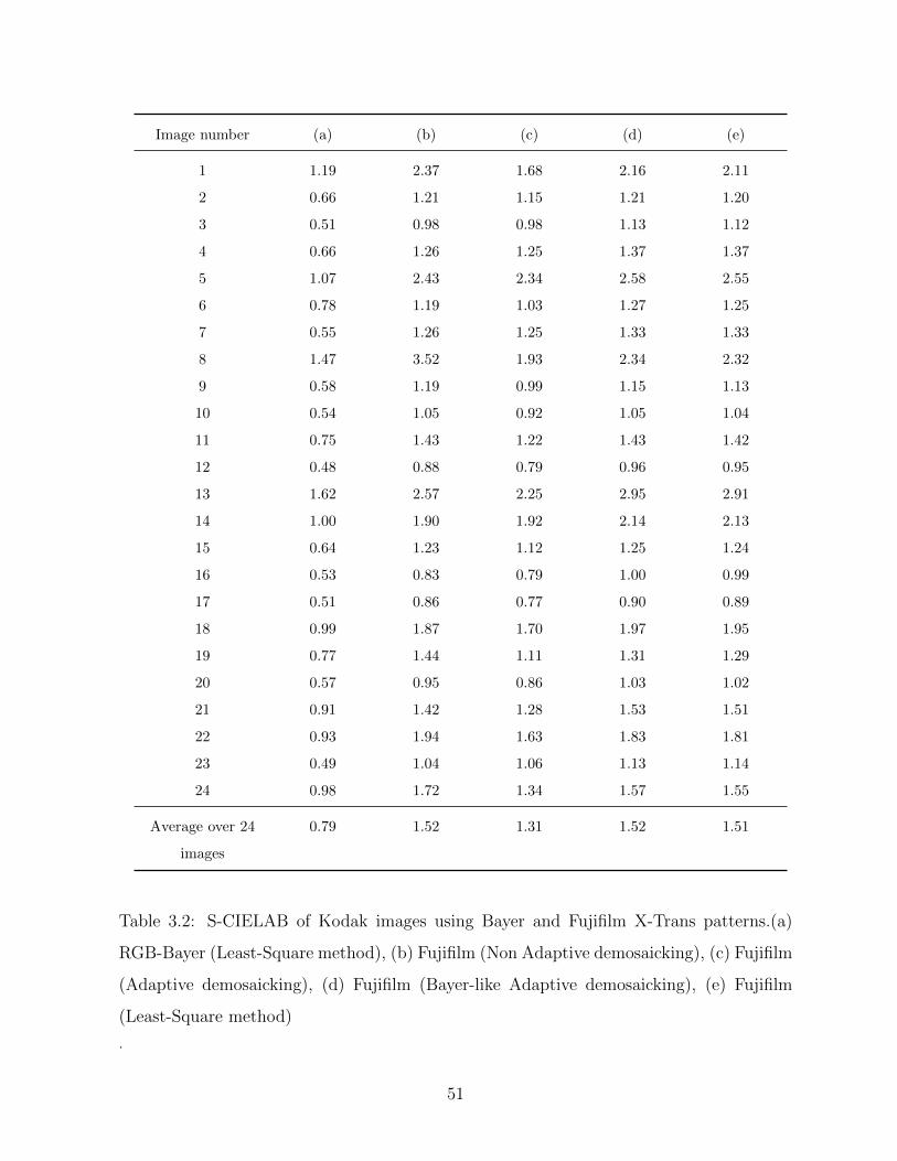
Image number (a) (b) (c) (d) (e)

1 1.19 2.37 1.68 2.16 2.11

2 0.66 1.21 1.15 1.21 1.20

3 0.51 0.98 0.98 1.13 1.12

4 0.66 1.26 1.25 1.37 1.37

5 1.07 2.43 2.34 2.58 2.55

6 0.78 1.19 1.03 1.27 1.25

7 0.55 1.26 1.25 1.33 1.33

8 1.47 3.52 1.93 2.34 2.32

9 0.58 1.19 0.99 1.15 1.13

10 0.54 1.05 0.92 1.05 1.04

11 0.75 1.43 1.22 1.43 1.42

12 0.48 0.88 0.79 0.96 0.95

13 1.62 2.57 2.25 2.95 2.91

14 1.00 1.90 1.92 2.14 2.13

15 0.64 1.23 1.12 1.25 1.24

16 0.53 0.83 0.79 1.00 0.99

17 0.51 0.86 0.77 0.90 0.89

18 0.99 1.87 1.70 1.97 1.95

19 0.77 1.44 1.11 1.31 1.29

20 0.57 0.95 0.86 1.03 1.02

21 0.91 1.42 1.28 1.53 1.51

22 0.93 1.94 1.63 1.83 1.81

23 0.49 1.04 1.06 1.13 1.14

24 0.98 1.72 1.34 1.57 1.55

Average over 24

images

0.79 1.52 1.31 1.52 1.51

Table 3.2: S-CIELAB of Kodak images using Bayer and Fujifilm X-Trans patterns.(a)

RGB-Bayer (Least-Square method), (b) Fujifilm (Non Adaptive demosaicking), (c) Fujifilm

(Adaptive demosaicking), (d) Fujifilm (Bayer-like Adaptive demosaicking), (e) Fujifilm

(Least-Square method)

.

51

3.4 Four channel color filter array

Most of the four channel CFAs contain red, green, blue and white/ panchromatic filters.

There are some other four channel CFAs like: RGBE and CYGM. RGBE is an alternative

for Bayer and one of the green pixels in Bayer has been modified to emerald. It has been

used in some Sony cameras. CYGM is used in a few cameras and it is a 2× 2 pattern with

one cyan, one yellow, one green, and one magenta. Figure 3.5 shows some sample four

channel patterns. White filters in RGBW patterns usually pass all the color spectrum and

the measured values through white filters can be estimated as a combination of red, green

and blue values.

Since the white filters receive more signal to noise ratio than color filters, we decided

to study the noise reduction impact on different RGBW patterns. The following sec-

tions present non-adaptive as well as adaptive demosaicking algorithms on RGBW-Bayer,

RGBW-Kodak and a proposed RGBW (5 × 5) in [45]. The optimized method using the

least square method is also provided for RGBW-Bayer, and the noise effect on this pattern

will be discussed in chapter 4.

Since most of standard datasets like Kodak dataset contain red, green and blue color

information, and they do not provide clear/panchromatic color information, we will esti-

mated the value of clear/panchromatic filters in three different ways as follows:

• Initially, the clear/panchromatic pixels value will be assumed as a combination of

equal amount of red, green and blue pixels values as W = 13R+ 1

3G+ 1

3B. Then the

CFA image will be calculated based on Kodak dataset for RGBW-Kodak, RGBW-

5× 5 and RGBW-Bayer patterns. The demosaicking algorithm will be designed and

tested on the CFA images of all three patterns. The results will be compared and

the best demosaicking algorithm using one of these CFA patterns will be chosen.

• Secondly, the clear/panchromatic pixels will be assumed as a linear combination of

red, green and blue pixel values with different coefficient. Those coefficients are not

necessarily equal. The panchromatic pixels will be estimated as W = αRR+ αGG+

αBB, and αR, αG and αB will be estimated using an optimization method over

52

(a) RGBW-Bayer pattern

(b) RGBE pattern

(c) RGBW-Kodak pattern

(d) CYGM pattern

Figure 3.5: Sample four channel CFA patterns

Macbeth color checker [37]. Then, the chosen CFA among three four-channel CFAs

will be calculated using the new set of coefficients, and the demosaicking algorithm

for the same CFA will be updated.

• Finally, the estimated clear/ panchromatic pixel values will be validated using a

hyperspectral image dataset. The red, green, blue and panchromatic pixels for the

chosen CFA will be calculated on the hyperspectral images, and the demosaicking

algorithm for the same CFA will be tested using hyperspectral image information.

53

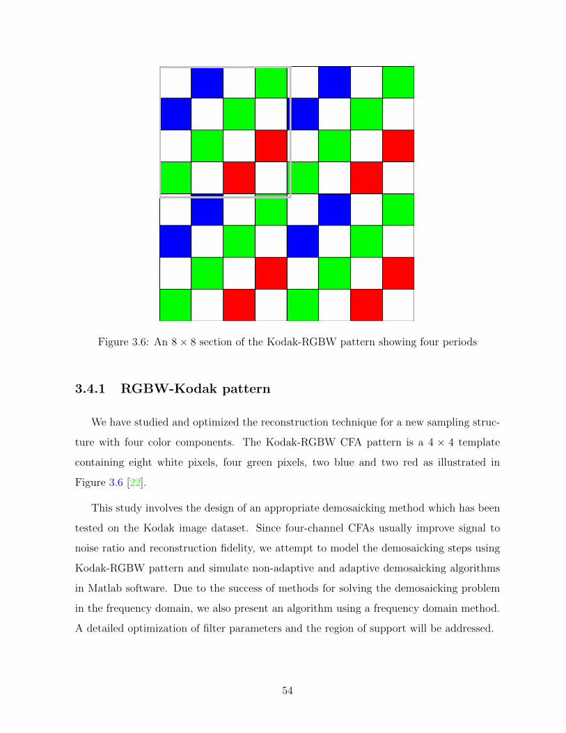
Figure 3.6: An 8× 8 section of the Kodak-RGBW pattern showing four periods

3.4.1 RGBW-Kodak pattern

We have studied and optimized the reconstruction technique for a new sampling struc-

ture with four color components. The Kodak-RGBW CFA pattern is a 4 × 4 template

containing eight white pixels, four green pixels, two blue and two red as illustrated in

Figure 3.6 [22].

This study involves the design of an appropriate demosaicking method which has been

tested on the Kodak image dataset. Since four-channel CFAs usually improve signal to

noise ratio and reconstruction fidelity, we attempt to model the demosaicking steps using

Kodak-RGBW pattern and simulate non-adaptive and adaptive demosaicking algorithms

in Matlab software. Due to the success of methods for solving the demosaicking problem

in the frequency domain, we also present an algorithm using a frequency domain method.

A detailed optimization of filter parameters and the region of support will be addressed.

54

Demosaicking algorithm

The CFA signal is sampled on lattice Λ = Z2 with reciprocal lattice Λ∗ = Z2. The

pattern is 4 × 4 and one period with respect to the periodicity lattice covers the sixteen

different points for each pixel. The periodicity lattice and corresponding reciprocal lattice

are given by:

VΓ =

4 0

0 4

, VΓ∗ =

14

0

0 14

. (3.63)

The demosaicking model that is used in this study has been described in [18] and we

modified it for RGBW-Kodak pattern. According to the analysis, the CFA signal can be

described as a sum of chroma and luma components.

fCFA[x] =K∑i=1

qi[x] exp(j2π(x · di)), K = 16 (3.64)

As we discussed in chapter 2, b i refers to the columns of matrix B which gives the coset

representatives of Γ in Λ. Also di refers to the columns of matrix D and they are coset

representatives of Λ∗ in Γ∗. The matrix D is a 2 × K matrix where K is the number

of components in one period of the lattice, which is equal to 16 for the RGBW-Kodak

pattern. We have used

D =1

4×

0 1 −1 0 0 1 −1 1 −1 2 0 2 −1 2 1 2

0 0 0 1 −1 1 −1 −1 1 0 2 −1 2 1 2 2

, (3.65)

B =

0 1 2 3 0 1 2 3 0 1 2 3 0 1 2 3

0 0 0 0 1 1 1 1 2 2 2 2 3 3 3 3

. (3.66)

The luma and chroma components can be extracted from the CFA image, so we can

calculate them using the following equation:

q [x] = Mf [x] (3.67)

f =[f1 , f2 , f3

]T, and q =

[q1 , q2 , ... , q16

]T(3.68)

55

The calculated matrix M for 16 components is shown below for Kodak-RGBW pattern.

M =

0.125 0.25 0.125 0.5

−0.0625 + 0.0625j 0 0.0625− 0.0625j 0

−0.0625− 0.0625j 0 0.0625 + 0.0625j 0

0.0625− 0.0625j 0 −0.0625 + 0.0625j 0

+0.0625 + 0.0625j 0 −0.0625− 0.0625j 0

0.125 −0.25 0.125 0

−0.125 0.25 −0.125 0

0 0 0 0

0 0 0 0

0 0 0 0

0 0 0 0

−0.0625 + 0.0625j 0 0.0625− 0.0625j 0

+0.0625− 0.0625j 0 −0.0625 + 0.0625j 0

−0.0625− 0.0625j 0 +0.0625 + 0.0625j 0

+0.0625 + 0.0625j 0 −0.0625− 0.0625j 0

−0.125 −0.25 −0.125 0.5

(3.69)

The matrix J is defining the four input channels: R,G,B and W , while each column of

the matrix represents one of the colors in this pattern.

J =

0 0 0 1 0 0 1 0 0 0 0 0 0 0 0 0

0 1 0 0 1 0 0 0 0 0 0 1 0 0 1 0

0 0 0 0 0 0 0 0 0 1 0 0 1 0 0 0

1 0 1 0 0 1 0 1 1 0 1 0 0 1 0 1

T

(3.70)

As we discussed before, we assumed to have three-channel CFA camera input and simulate

the values of the white filter in the CFA image. Ideally the white filter should pass all three

colors and does not absorb any color spectrum. So the value of the white pixels in CFA

image can be estimated as W = 13R + 1

3G + 1

3B. This research is trying to show that the

captured panchromatic filter values in digital cameras usually contain less noise compared

to the other three color filters. This hypothesis will be discussed in presence of noise in

56

Figure 3.7: Luma- Chroma position in one unit cell for RGBW-Kodak pattern

Chapter 4.

W =1

3(R +B +G) (3.71)

In the frequency domain, the Fourier transform of the CFA signal is given by:

FCFA(u) =16∑i=1

Qi(u− di) Where Qi(u) , F{qi[x]} (3.72)

The chroma components are extracted with bandpass filters centered at the frequencies di.

The next step in the non-adaptive demosaicking algorithm is reconstructing the full RGB

color image using the pseudo inverse matrix M † and extracted chromas using the following

equation. Figure 3.7 shows the position of 16 extracted component in one unit cell of Λ∗.

Since we cannot fully extract the luma and chromas close to luma, those chromas can be

reconstructed using the rest of the components.

f [x] = M †q [x] (3.73)

Based on the matrix M , q2 to q5 and q12 to q15 can be reconstructed by using only one of

them. Also matrix M shows that the values of components q8 to q11 are zero.

Usually we are able to better extract the components which are further from the luma,

and we prefer to use the information of those components to reconstruct the other com-

ponents which are closer to the luma to avoid overlapping effects between luma and the

57

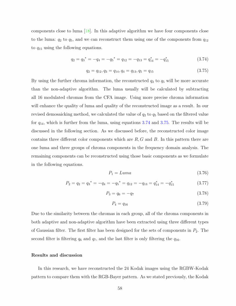
components close to luma [18]. In this adaptive algorithm we have four components close

to the luma: q2 to q5, and we can reconstruct them using one of the components from q12

to q15 using the following equations.

q2 = q3∗ = −q4 = −q5

∗ = q12 = −q13 = q∗14 = −q∗15 (3.74)

q2 = q12, q3 = q14, q4 = q13, q5 = q15 (3.75)

By using the further chroma information, the reconstructed q2 to q5 will be more accurate

than the non-adaptive algorithm. The luma usually will be calculated by subtracting

all 16 modulated chromas from the CFA image. Using more precise chroma information

will enhance the quality of luma and quality of the reconstructed image as a result. In our

revised demosaicking method, we calculated the value of q2 to q5 based on the filtered value

for q14, which is further from the luma, using equations 3.74 and 3.75. The results will be

discussed in the following section. As we discussed before, the reconstructed color image

contains three different color components which are R,G and B. In this pattern there are

one luma and three groups of chroma components in the frequency domain analysis. The

remaining components can be reconstructed using those basic components as we formulate

in the following equations.

P1 = Luma (3.76)

P2 = q2 = q3∗ = −q4 = −q5

∗ = q12 = −q13 = q∗14 = −q∗15 (3.77)

P3 = q6 = −q7 (3.78)

P4 = q16 (3.79)

Due to the similarity between the chromas in each group, all of the chroma components in

both adaptive and non-adaptive algorithm have been extracted using three different types

of Gaussian filter. The first filter has been designed for the sets of components in P2. The

second filter is filtering q6 and q7, and the last filter is only filtering the q16.

Results and discussion

In this research, we have reconstructed the 24 Kodak images using the RGBW-Kodak

pattern to compare them with the RGB-Bayer pattern. As we stated previously, the Kodak

58

dataset are white balanced and gamma corrected, so we only apply the demosaicking

algorithm on the input Kodak images, and the results compare the reconstructed images

with the input images as ground truth images.

Tables 3.3 and 3.4 show the PSNR and S-CIELAB comparison between the least-squares

luma- chroma demultiplexing (LSLCD) method using the Bayer CFA, and the revised and

non-adaptive demosaicking schemes using the RGBW-Kodak pattern over Kodak dataset

as well as the average PSNR over 24 Kodak images.

According to the presented results, the proposed revised demosaicking scheme using the

RGBW-Kodak pattern largely improved the results of the non-adaptive algorithm using the

same pattern. The tables also show the comparison between the least-squares optimized

method using RGB-Bayer pattern and our revised method using RGBW-Kodak pattern.

Also Figure 3.8 provides the reconstructed images using the mentioned patterns and the

original images. The results show some improvements mostly in horizontal and vertical

axes using RGBW-Kodak. The reconstructed images contain fewer false colors in different

axes using our algorithm compared to the RGB-Bayer pattern, while the least-squares

method using the Bayer pattern reconstructs the edge details more accurately.

59

(a) Original image (b) Reconstructed

using RGB-Bayer

(c) Reconstructed

using RGBW-

Kodak

Figure 3.8: Comparison between the revised method using RGBW-Kodak and LSLCD

method using RGB-Bayer

60

Kodak image number RGB LSLCD method RGBW-

Kodak(Revised

demosaicking)

RGBW-Kodak(Non-

Adaptive

demosaicking)

1 37.92 36.33 27.12

2 40.65 36.10 33.55

3 42.22 36.67 34.74

4 41.09 35.86 34.10

5 37.92 31.90 29.06

6 39.95 38.56 29.55

7 42.52 36.35 33.83

8 35.32 34.02 24.56

9 42.57 37.93 32.25

10 42.63 38.74 33.83

11 39.81 36.36 30.84

12 43.14 39.13 33.27

13 34.20 33.02 27.54

14 36.77 30.83 29.37

15 39.83 35.76 33.21

16 43.63 41.25 33.01

17 41.63 38.68 34.54

18 37.28 34.01 30.46

19 40.53 38.06 28.52

20 40.97 37.45 32.06

21 38.79 36.69 30.02

22 38.57 34.82 31.01

23 42.98 36.40 34.29

24 35.34 35.27 30.12

Average over 24

images

39.8 36.3 31.3

Table 3.3: PSNR of Kodak images using RGB-Bayer (least-square method) and RGBW-

Kodak (Non-adaptive and Revised method) and the average PSNR over 24 Kodak images

61

Kodak image number RGB LSLCD method RGBW-

Kodak(Revised

demosaicking)

RGBW-Kodak(Non-

Adaptive

demosaicking)

1 1.19 2.24 4.96

2 0.66 1.28 1.94

3 0.66 1.27 1.87

4 0.66 1.57 2.03

5 1.07 3.45 4.09

6 0.78 1.49 3.44

7 0.55 1.70 2.20

8 1.47 2.63 5.99

9 0.58 1.37 2.41

10 0.54 1.24 2.06

11 0.75 1.67 2.80

12 0.48 1.07 2.18

13 1.62 3.28 4.95

14 1.00 2.60 3.38

15 0.64 1.47 2.04

16 0.53 1.10 2.34

17 0.51 1.16 1.71

18 0.99 2.44 3.13

19 0.77 1.57 3.15

20 0.57 1.17 2.29

21 0.91 1.89 3.28

22 0.93 2.23 3.16

23 0.49 1.44 1.81

24 0.98 2.06 3.30

Average over 24

images

0.79 1.81 2.94

Table 3.4: S-CIELAB of Kodak images using RGB-Bayer (least-square method) and

RGBW-Kodak (Non-adaptive and Revised method) and the average S-CIELAB over 24

Kodak images

62

Figure 3.9: RGBW(5× 5)[45] (four periods)

3.4.2 RGBW - 5× 5 pattern

The 5 × 5 RGBW CFA has been proposed in [45] and the demosaicking algorithm

presented in [29] has been implemented on it. We are presenting some improvement on

the result of the reconstructed images using this pattern with the same demosaicking

algorithm. Figure 3.9 shows a new proposed RGBW CFA in [45]. This CFA is a 5 × 5

template containing 10 white pixel and equal number of red, green and blue filters.

Demosaicking algorithm

As we can see in Figure 3.10 a smaller pattern containing five pixels is repeated in

this CFA. Using the smaller pattern, the CFA signal is sampled on lattice Λ = Z2 with

reciprocal lattice Λ∗ = Z2. The periodicity lattice and corresponding reciprocal lattice are

63

Figure 3.10: The smaller repeated pattern in RGBW(5× 5)

given by:

VΓ =

2 −1

1 2

, VΓ∗ =

25−15

15

25

(3.80)

Using these lattices, we can model the CFA signal as a sum of luma and chroma compo-

nents. The demosaicking model is presented in Chapter 2, and it is modified here for this

pattern.

fCFA[x] =K∑i=1

qi[x] exp(j2π(x · di)), (3.81)

K = 5 (3.82)

As we discussed in Chapter 2, matrix B and matrix D for this CFA pattern are as follows.

B =

0 1 2 0 1

0 0 0 1 1

, (3.83)

D =1

5×

0 2 −2 −1 1

0 1 −1 2 −2

, (3.84)

Also matrix M will be calculated using the following equations.

q [x] = Mf [x] (3.85)

f =[f1, f2, f3

]T(3.86)

q =[q1, q2, ... , q5

]T64

K = 5 (3.87)

M (RGBW5×5) =

0.2 0.2 0.2 0.4

−0.1618− 0.1176j −0.1618 + 0.1176j 0.0618 + 0.1902j 0.2618− 0.1902j

−0.1618 + 0.1176j −0.1618− 0.1176j 0.0618− 0.1902j 0.2618 + 0.1902j

0.0618 + 0.1902j 0.0618− 0.1902j −0.1618 + 0.1176j 0.0382− 0.1176j

0.0618− 0.1902j 0.0618 + 0.1902j −0.1618 + 0.1176j 0.0382− 0.1176j

(3.88)

The matrix J is a 5 × 4 matrix, as we explained in Chapter 2, and it defines four input

channels: R, G, B and W. The values of the white filter in the CFA image will be calculated

as W = 13R + 1

3G+ 1

3B.

JRGBW5×5 =

0 0 0 1

1 0 0 0

0 0 1 0

0 0 0 1

0 1 0 0

T

(3.89)

W =1

3(R +B +G) (3.90)

In the frequency domain, the Fourier transform of the CFA signal is:

FCFA(u) =K∑i=1

Qi(u− di) Where Qi(u) , F{qi[x]} (3.91)

The chroma components are extracted with bandpass filters centered at the frequencies

di. The next step in the non-adaptive demosaicking algorithm is reconstructing the full

RGB color image using the pseudo inverse matrix M †. Figure 3.11 shows the position of 5

extracted component in one unit cell of Λ∗. Since we reduce the number of repeated color

filters from 25 to 5, there is four chroma components with the same Euclidean distance

of the luma in one unit cell. Thus, there is no other way to isolate the chromas from the

luma, and enhance the quality of the reconstructed chromas with an adaptive algorithm.

Results and discussion

The demosaicking method has been applied on the input Kodak images as previous

sections, and the PSNR results calculate the difference between reconstructed images and

65

Figure 3.11: Luma- Chroma position in one unit cell-RGBW(5× 5)

the input images. Although the method discussed in [45] is using the same demosaicking

approach, our implemented algorithm improved the PSNR slightly and the visual results

also shows some improvement in color estimation. Table 3.5 shows the comparison between

our method and the proposed method in [45] using RGBW 5×5 as well as the non-adaptive

demosaicking algorithm using RGBW-Bayer that will be discuss in the next section.

66

Image number in

dataset

RGBW(5× 5)

proposed

Non-Adaptive

demosaicking)

RGBW(5× 5)

reconstructed in [45]

using Dubois Method

1 36.56 35.23

2 37.05 37.49

3 37.46 37.46

4 37.21 37.32

5 33.47 32.96

6 38.88 36.56

7 37.94 38.22

8 34.35 33.28

9 38.84 38.78

10 37.77 36.63

11 37.01 36.13

12 40.39 40.18

13 32.93 30.91

14 31.87 32.24

15 36.65 36.29

16 40.98 39.58

17 39.24 37.90

18 34.79 33.87

19 38.58 37.53

20 37.58 36.71

21 37.31 36.14

22 35.81 35.59

23 38.04 38.86

24 35.27 31.90

Average over 24

images

36.9 35.4

Table 3.5: PSNR of proposed Non-Adaptive demosaicking method using RGBW(5 × 5)

pattern and the presented method in [45] for Kodak dataset

67

3.4.3 RGBW-Bayer pattern

Figure 3.12 shows the RGBW-Bayer pattern. The RGBW-Bayer period contains four

pixels, and is the same as the RGB-Bayer pattern where one of the green filters has been

replaced with a white pixel.

Figure 3.12: RGBW-Bayer pattern

Demosaicking algorithm

The CFA signal is sampled on lattice Λ = Z2 with reciprocal lattice Λ∗ = Z2. The

periodicity lattice and corresponding reciprocal lattice are given by:

VΓ =

2 0

0 2

, VΓ∗ =

12

0

0 12

(3.92)

Using the mentioned lattices, we can model the CFA signal as a sum of luma and chroma

components. The demosaicking model described in [18] has been used and modified here.

fCFA[x] =K∑i=1

qi[x] exp(j2π(x · di))), (3.93)

K = 4 (3.94)

According to [18], bi refers to the columns of matrix B which gives the coset representative

of Γ in Λ. Also di refers to the columns of matrix D and they are coset representatives of

68

Λ∗ in Γ∗.

B =

0 1 0 1

0 0 1 1

, (3.95)

The matrix D is a 2 ×K matrix where K is the number of components in one period of

the lattice, which is equal to 4 in RGBW-Bayer.

D =1

2×

0 1 0 1

0 0 1 1

, (3.96)

The luma and chroma components can be extracted from the CFA image, so we can

calculate the M using the following equation.

q [x] = Mf [x] (3.97)

f =[f1, f2, f3

]T(3.98)

q =[q1, q2, q3, q4

]TThe calculated matrices M for each CFA are as follow.

M Bayer =

0.25 0.25 0.25 0.25

−0.25 0.25 0.25 −0.25

0.25 0.25 −0.25 −0.25

−0.25 0.25 −0.25 0.25

(3.99)

The matrix J is defining the four input channels: R, G, B and W, while each column of

the matrix represents one of the colors in this pattern. As we discussed before, we assume

that the white filter should pass all three colors and does not absorb any color spectrum.

So the value of the white pixels in CFA image can be estimated as the summation of R,

G and B divided by three. The value that has been captured by the white filter usually

contains less noise compared the other three color filters and the optimized results of this

study can be used for noise reduction purposes in the future.

JBayer =

0 1 0 0

1 0 0 0

0 0 1 0

0 0 0 1

T

(3.100)

69

The chroma components are filtered using bandpass filters centered at the frequencies di.

The full color image will be reconstructed using matrix M † in the non-adaptive demo-

saicking algorithm. Figure 3.13 shows the luma-chroma position in one unit cell.

Figure 3.13: Luma- Chroma position in one unit cell for RGBW-Bayer

Adaptive demosaicking algorithm for RGBW-Bayer pattern

Note that with our first assumption about W = 13(R + B + G), we can simplify our

initial implementations as follows:

f4(x) =1

3(f1(x) + f2(x) + f3(x)) (3.101)

So we can recalculate all chromas.

q1(x) =1

3(f1(x) + f2(x) + f3(x)) (3.102)

q2(x) =1

3(f1(x) +

1

2f2(x) +

1

2f3(x)) (3.103)

q3(x) =1

3(1

2f1(x) +

1

2f2(x)− f3(x)) (3.104)

q4(x) =1

3(−1

2f1(x) + f2(x)− 1

2f3(x)) (3.105)

70

In matrix form q1(x)

q2(x)

q3(x)

q4(x)

=

13

13

13

−13

16

16

16

16−1

3

−16

13−1

6

f1(x)

f2(x)

f3(x)

(3.106)

where the coefficient matrix called M. Also we have:

fCFA(x, y) = q1(x, y) + q2(x, y)(−1)x + q3(x, y)(−1)y + q4(x, y)(−1)x+y (3.107)

= r1(x, y) + r2(x, y) + r3(x, y) + r4(x, y) (3.108)

As we can see in the matrix M, 4th row of matrix M is sum of 2nd and 3rd rows. So:

q2(x, y) + q3(x, y) = q4(x, y) (3.109)

For the adaptive algorithm, first we need to estimate r2, r3, r4 with three bandpass filters

at (12, 0), (0, 1

2), (1

2, 1

2) respectively. Then demodulate them as follows:

q2(x, y) = r2(x, y)(−1)x (3.110)

q3(x, y) = r3(x, y)(−1)y (3.111)

q4(x, y) = r4(x, y)(−1)x+y (3.112)

Then we need to find the average energy, as we discussed before. Assuming the calculated

energy near (fm, 0), (0, fm) is ex and ey, we can set

w =ex

ex + ey(3.113)

When w ≈ 1, then q2 is more reliable, and when w ≈ 0, then q3 is more reliable. Therefore,

if w ≈ 1, we leave q2 as it is, and replace q3 with q4 − q2 using equation 3.109. If w ≈ 0,

we leave q3 as it is, and replace q2 with q4 − q3.

In general, the reconstructed chromas can be express as:

q2(x) = w(x)q2(x) + (1− w(x))(q4(x)− q3(x)) (3.114)

q3(x) = (1− w(x))q3(x) + w(x)(q4(x)− q2(x)) (3.115)

71

q4(x) = q4(x), no change (3.116)

Using the new value of the reconstructed chromas, we can estimate luma.

q1(x, y) = fCFA(x, y)− q2(x, y)(−1)x − q3(x, y)(−1)y − r4(x, y) (3.117)

So, the M† matrix will be as follows:

M† =

1 −4

323−2

3

1 23

23

43

1 23−4

3−2

3

(3.118)

And we can reconstruct the RGB image using M † matrix.

Results and discussion

In this section the results of adaptive demosaicking using RGBW-Bayer have been com-

pared with the least square method using RGB-Bayer. The Kodak dataset is used as the

input images, and the CFA is reconstructed using them. Then the proposed demosaicking

algorithm will be applied on the CFA images afterward. The PSNR ans S-CIELAB metrics

are applied to compare the input Kodak images and the reconstructed images using the

proposed demosaicking algorithm. Table 3.6 and 3.7 shows the comparison between three-

channel and four-channel Bayer patterns in term of PSNR and S-CIELAB. The results are

very close in both CFAs for the noise-free images.

72

Image number in

dataset

Bayer-RGBW

(Adaptive

demosaicking)

RGB-Bayer (LSLCD

method)[29]

1 37.90 37.92

2 39.22 40.65

3 40.82 42.22

4 40.02 41.09

5 36.93 37.92

6 43.64 39.95

7 41.21 42.52

8 34.92 35.32

9 41.48 42.57

10 41.84 42.63

11 39.29 39.81

12 42.92 43.14

13 34.87 34.20

14 34.82 36.77

15 39.16 39.83

16 43.80 43.63

17 41.31 41.63

18 36.73 37.28

19 40.13 40.53

20 40.17 40.97

21 38.65 38.79

22 37.46 38.57

23 41.12 42.98

24 39.36 35.34

Average over 24 images 39.49 39.8

Table 3.6: Comparison between the PSNR of Adaptive demosaicking method using RGBW-

Bayer CFA and Least Square method using RGB-Bayer for Kodak dataset

73

Image number in

dataset

Bayer-RGBW

(Adaptive

demosaicking)

RGB-Bayer (LSLCD

method)[29]

1 1.25 1.19

2 0.74 0.66

3 0.62 0.51

4 0.76 0.66

5 1.34 1.07

6 0.44 0.78

7 0.69 0.55

8 1.59 1.47

9 0.69 0.58

10 0.65 0.54

11 0.85 0.75

12 0.53 0.48

13 1.69 1.62

14 1.21 1.00

15 0.75 0.64

16 0.58 0.53

17 0.56 0.51

18 1.19 0.99

19 0.87 0.77

20 0.64 0.57

21 1.01 0.91

22 1.08 0.93

23 0.62 0.49

24 0.56 0.98

Average over 24 images 0.87 0.79

Table 3.7: Comparison between the S-CIELAB of Adaptive demosaicking method using

RGBW-Bayer and Least Square method using RGB-Bayer for Kodak dataset

74

3.4.4 Comparison between RGBW patterns

In this research we decided to develop a demosaicking algorithm for RGBW CFAs, and

study on the effect of clear/panchromatic pixels in reconstructed image quality. Three

different four channel CFAs have been studied, and a demosaicking algorithm has been

developed for each case. The Kodak data set is used to evaluate and compare the results.

Table 3.8 and 3.9 show the PSNR and S-CIELAB comparison between non-adaptive

demosaicking algorithm for each CFA as well as the results of PSNR of the previous work

using RGBW 5 × 5 [45] on Kodak images and the average over 24 Kodak dataset. Also

Table 3.10 illustrates the PSNR comparison between adaptive demosaicking results for

RGBW-Bayer and RGBW-Kodak [39] for the same sample images. The results have been

compared with the results of Least-Square method on the RGB-Bayer [29].

The results of Table 3.8 and 3.9 show the non-adaptive demosaicking method that we

proposed for RGBW(5× 5) improved the PSNR and S-CIELAB comparing to the method

in [45]. Also the result of non-adaptive method using RGBW-Bayer is also working slightly

better among three discussed RGBW patterns.

75

(a) Original image

(b) Non-adaptive

RGBW-Kodak

(c) RGBW CFA(5×

5)

(d) Adaptive

RGBW-Kodak

(e) Non-Adaptive

RGBW-Bayer

(f) Adaptive

RGBW-Bayer

(g) Least Square

RGB-Bayer [16]

Figure 3.14: Comparison between The adaptive and non-adaptive demosaicking method

for different four channel CFAs

76

Image number in

dataset

Bayer-RGBW

(Non-Adaptive

demosaicking)

Kodak-RGBW

(Non-Adaptive

demosaicking)

RGBW(5× 5)

proposed

Non-Adaptive

demosaicking)

RGBW(5× 5)

reconstructed in

[45] using Dubois

Method

1 36.14 27.12 36.56 35.23

2 36.74 33.55 37.05 37.49

3 37.88 34.74 37.46 37.46

4 37.25 34.10 37.21 37.32

5 34.20 29.06 33.47 32.96

6 39.15 29.55 38.88 36.56

7 37.92 33.83 37.94 38.22

8 32.27 24.56 34.35 33.28

9 38.51 32.25 38.84 38.78

10 39.58 33.83 37.77 36.63

11 37.17 30.84 37.01 36.13

12 39.58 33.27 40.39 40.18

13 35.09 27.54 32.93 30.91

14 31.85 29.37 31.87 32.24

15 37.07 33.21 36.65 36.29

16 40.26 33.01 40.98 39.58

17 40.34 34.54 39.24 37.90

18 35.62 30.46 34.79 33.87

19 37.09 28.52 38.58 37.53

20 38.24 32.06 37.58 36.71

21 37.21 30.02 37.31 36.14

22 35.49 31.01 35.81 35.59

23 37.80 34.29 38.04 38.86

24 37.06 30.12 35.27 31.90

Average over 24

images

37.06 31.3 36.9 35.42

Table 3.8: PSNR for Non-Adaptive demosaicking method using different RGBW patterns

and the average PSNR over 24 Kodak images

77

Image number in

dataset

Bayer-RGBW

(Non-Adaptive

demosaicking)

Kodak-RGBW

(Non-Adaptive

demosaicking)

RGBW(5× 5) proposed

Non-Adaptive

demosaicking)

1 1.96 4.96 2.03

2 1.09 1.94 1.04

3 0.96 1.87 1.17

4 1.07 2.03 1.19

5 1.95 4.09 2.40

6 1.18 3.44 1.32

7 1.14 2.20 1.22

8 2.46 5.99 2.37

9 1.04 2.41 1.09

10 0.93 2.06 1.18

11 1.32 2.80 1.40

12 0.94 2.18 0.88

13 1.98 4.95 2.88

14 1.79 3.38 2.15

15 1.02 2.04 1.13

16 1.15 2.34 1.07

17 0.70 1.71 0.89

18 1.55 3.13 1.95

19 1.35 3.15 1.28

20 0.92 2.29 1.05

21 1.41 3.28 1.52

22 1.56 3.16 1.68

23 0.98 1.81 1.02

24 1.06 3.30 1.62

Average over 24

images

1.31 2.94 1.48

Table 3.9: S-CIELAB of some sample images for Non-Adaptive demosaicking method using

different RGBW patterns and the average S-CIELAB over 24 Kodak images

78

The Tables 3.10 and 3.11 provide the results of adaptive demosaicking algorithm in

terms of PSNR and S-CIELAB, and show some improvement on the proposed adaptive

demosaicking algorithm using the RGBW-Bayer comparing to the adaptive algorithm using

RGBW-Kodak. The results have also been compared with the least-square method results

on RGB-Bayer pattern.

Usually adaptive demosaicking method reconstruct more isolated chroma and luma

signals and works better than non adaptive methods, and the reconstructed images prove

this fact. As we can see in Figure 3.14, among non-adaptive methods, the RGBW(5× 5)

is more successful to estimate colors correctly while RGBW-Bayer reconstruct the edges

and image details better.

Comparing adaptive algorithms, the RGBW-Kodak fully estimated the colors. The

proposed weighted algorithm for RGBW-Bayer reconstructs the image details better while

it contains some false color. We can conclude that the CFA templates with more white

filters estimate less false color and an appropriate adaptive demosaicking algorithm is

needed to restore the edges perfectly.

79

Image number in

dataset

Bayer-RGBW

(Adaptive

demosaicking)

Kodak-RGBW

(Adaptive

demosaicking)

RGB-Bayer (LSLCD

method)[1]

1 37.90 36.33 37.92

2 39.22 36.10 40.65

3 40.82 36.67 42.22

4 40.02 35.84 41.09

5 36.93 31.90 37.92

6 43.64 38.56 39.95

7 41.21 36.35 42.52

8 34.92 34.02 35.32

9 41.48 37.93 42.57

10 41.84 38.74 42.63

11 39.29 36.36 39.81

12 42.92 39.13 43.14

13 34.87 33.02 34.20

14 34.82 30.83 36.77

15 39.16 35.76 39.83

16 43.80 41.25 43.63

17 41.31 38.68 41.63

18 36.73 34.01 37.28

19 40.13 38.06 40.53

20 40.17 37.45 40.97

21 38.65 36.69 38.79

22 37.46 34.82 38.57

23 41.12 36.40 42.98

24 39.36 35.27 35.34

Average over 24

images

39.4 36.3 39.8

Table 3.10: Comparison between the PSNR of Kodak images for adaptive demosaicking

method using RGBW CFAs and least-square method using RGB-Bayer

80

Image number in

dataset

Bayer-RGBW

(Adaptive

demosaicking)

Kodak-RGBW

(Adaptive

demosaicking)

RGB-Bayer (LSLCD

method)[1]

1 1.25 2.24 1.19

2 0.74 1.28 0.66

3 0.62 1.27 0.51

4 0.76 1.57 0.66

5 1.34 3.45 1.07

6 0.44 1.49 0.78

7 0.69 1.70 0.55

8 1.59 2.63 1.47

9 0.69 1.37 0.58

10 0.65 1.24 0.54

11 0.85 1.67 0.75

12 0.53 1.07 0.48

13 1.69 3.28 1.62

14 1.21 2.60 1.00

15 0.75 1.47 0.64

16 0.58 1.10 0.53

17 0.56 1.16 0.51

18 1.19 2.44 0.99

19 0.87 1.57 0.77

20 0.64 1.17 0.57

21 1.01 1.89 0.91

22 1.08 2.23 0.93

23 0.62 1.44 0.49

24 0.56 2.06 0.98

Average over 24

images

0.87 1.81 0.79

Table 3.11: Comparison between the S-CIELAB of Kodak images for demosaicking method

using RGBW CFAs and least-square method using RGB-Bayer

81

3.4.5 White filter estimation

The method described in previous sections was based on W = 13R + 1

3G + 1

3B. We

optimized the white color component calculation assuming that there is a linear relationship

between white component and the three primary color components (red, green, blue).

The following method describes the closest way that we can linearly model white color

components similar to the digital cameras based on two different sensor characteristics.

VEML6040 is an available sensor released in 2015 from Vishay company [10], and KAI-

Kodak110002 [9] is a color sensor presented by Eastman Kodak company in 2004. We

will calculate the optimized coefficients separately for each sensor. Figure 3.15 shows a

typical non-normalized responsivity of red, green, blue and white filter spectral responses,

according to the VEML6040 sensor [10]. Also, Figure 3.16 shows responsivity curves of

red, green and blue filters for KAI-Kodak110002 [9], and Figure 3.17 is the responsivity

curve for white filter for the same sensor.

82

Figure 3.15: Non-normalized spectral response of red, green, blue and white color filters

for VEML6040 sensor (400nm-800nm)

83

Figure 3.16: Non-normalized spectral response of red, green and blue color filters for KAI-

Kodak11002 sensor (400nm-800nm)

84

Figure 3.17: Non-normalized spectral response of white filter for KAI-Kodak11002 sensor

(400nm-800nm)

85

Assuming a constant patch of light with power density spectrum C(λ), we make the

following four measurements over the range of wavelengths from 400 to 650 nm:

CR =

∫v

r(λ)C(λ)dλ (3.119)

CB =

∫v

b(λ)C(λ)dλ (3.120)

CG =

∫v

g(λ)C(λ)dλ (3.121)

CW =

∫v

w(λ)C(λ)dλ (3.122)

r(λ), g(λ), b(λ) and w(λ) are the spectral sensitivity curves of an RGBW CFA sensor.

Assume that r(λ), g(λ), b(λ) and w(λ) have been scaled, so that if C(λ) = D65(λ) with

luminance equal to 1, then DR = DB = DG = DW = 1. So the values of red, green, blue

and white components will be normalized by multiplying them to the spectrum of D65, as

a constant power density spectrum, on a specific range of wavelength. We wish to estimate

CW as a linear combination of CR, CG, CB:

CW = aRCR + aGCG + aBCB, where aR + aG + aB = 1 (3.123)

Then using a database of typical spectral densities of light, we can calculate and minimize

the mean square error between the real white components and the calculated one. We

calculate and normalized the values of red (CR), green (CG), blue (CB) and white (CW )

over the Macbeth color checker database [37].

Common light sources deliver light that has a very broad spectral output, reaching

beyond the visible, so many visual and detector-based applications use an infrared filter

that is designed to pass only light within the visible spectrum. Thus, there is an IR cut-off

filter inside digital cameras that eliminates the effects of infrared light, and cuts off the

frequencies over 650 nm. Therefore we filtered the values over 650 nm in our simulation.

The MSE will be calculated for both sensors separately, using the Quadratic program-

ming subject to aR + aB + aG = 1.

Error =N∑i=1

(CW i − (aRCRi + aGCGi + aBCBi))2 (3.124)

86

N = number of samples in the database

Using Lagrange multiplier method, we can minimize error function subject to aR+aB+aG =

1. We set β as Lagrange multiplier variable, and find the local minimum of the ε function.

ε =N∑i=1

(CW i − (aRCRi + aGCGi + aBCBi))2 + β(aR + aB + aG) (3.125)

∇aR =∂ε

∂aR=

N∑i=1

2(CW i − (aRCRi + aGCGi + aBCBi))(−CRi) + β = 0 (3.126)

∇aG =∂ε

∂aR=

N∑i=1

2(CW i − (aRCRi + aGCGi + aBCBi))(−CGi) + β = 0 (3.127)

∇aB =∂ε

∂aR=

N∑i=1

2(CW i − (aRCRi + aGCGi + aBCBi))(−CBi) + β = 0 (3.128)

We can show all three equations in matrix form.2∑N

i=1CRi2 2

∑Ni=1CRiCGi 2

∑Ni=1CRiCBi

2∑N

i=1CGiCRi 2∑N

i=1CGi2 2

∑Ni=1CGiCBi

2∑N

i=1CBiCRi 2∑N

i=1 CBiCGi 2∑N

i=1 CBi2

aR

aG

aB

=

2∑N

i=1 CW iCRi

2∑N

i=1CW iCGi

2∑N

i=1CW iCBi

−β

1

1

1

(3.129)

Assuming

Q =

2∑N

i=1 CRi2 2

∑Ni=1CRiCGi 2

∑Ni=1CRiCBi

2∑N

i=1CGiCRi 2∑N

i=1CGi2 2

∑Ni=1 CGiCBi

2∑N

i=1CBiCRi 2∑N

i=1 CBiCGi 2∑N

i=1CBi2

(3.130)

and

b =

2∑N

i=1CW iCRi

2∑N

i=1 CW iCGi

2∑N

i=1 CW iCBi

(3.131)

we can simplify the equation as:aR

aG

aB

= Q−1(b− β

1

1

1

) (3.132)

87

Using the constraint, we can find β, and apply it to the problem. The local minimum

values for aR, aB and aG will be estimated.

[1 1 1

]aR

aG

aB

= 1 (3.133)

β =

[1 1 1

]Q−1b− 1

[1 1 1

]Q−1

1

1

1

(3.134)

The calculated aR, aB and aG will be replaced in equation 3.90 as coefficients for red, green

and blue components. The calculated values based on VEML6040 sensor are aR = 0.3870,

aG = 0.2571 and aB = 0.3560. Note that these coefficients will be applied to a camera

using the filters shown in Figure 3.15.

WVEML6040 = 0.3870(R) + 0.2571(G) + 0.3560(B) (3.135)

Same coefficients have been calculated for KAI-Kodak11002 sensor as aR = 0.1783, aG =

0.3864 and aB = 0.4353, and these coefficients will be applied to a camera using filters as

Figure 3.16 and 3.17.

WKAI-Kodak11002 = 0.1783(R) + 0.3864(G) + 0.4353(B) (3.136)

88

Updated demosaicking algorithm for RGBW-Bayer

In this section, the presented adaptive demosaicking algorithm will be updated using

the new sets of coefficients for both sensors. For VEML6040 sensor as the white filter

values in the CFA have been updated using equation 3.135, the adaptive demosaicking

algorithm for RGBW-Bayer pattern has been designed based on the new white values.

f4(x) = 0.3870f1(x) + 0.2571f2(x) + 0.3560f3(x) (3.137)

So we can recalculate all chromas as follows:

q1(x) =1

4((1 + aR)f1(x) + (1 + aG)f2(x) + (1 + aB)f3(x)) (3.138)

q2(x) =1

4((−1− aR)f1(x) + (1− aG)f2(x) + (1− aB)f3(x)) (3.139)

q3(x) =1

4((1− aR)f1(x) + (1− aG)f2(x) + (−1− aB)f3(x)) (3.140)

q4(x) =1

4((−1 + aR)f1(x) + (1 + aG)f2(x) + (−1 + aB)f3(x)) (3.141)

In matrix form q1(x)

q2(x)

q3(x)

q4(x)

=

0.3234 0.3726 0.3040

−0.3234 0.1274 0.1960

0.1766 0.1274 −0.3040

−0.1766 0.3726 −0.1960

f1(x)

f2(x)

f3(x)

(3.142)

As matrix M’ has been updated with equation 3.137, we can call the updated coefficients

matrix as N.

We will use the same weighting scheme described in the previous section. The updated

reconstructed chromas using weighting scheme can be express as

q2weighted(x) = w(x)q2(x) + (1− w(x))(0.4348

0.6028q4(x)− 0.6690

0.6028q3(x)) (3.143)

q3weighted(x) = (1− w(x))q3(x) + w(x)(0.4348

0.6690q4(x)− 0.6028

0.6690q2(x)) (3.144)

q4(x) = q4(x), no change (3.145)

89

Also, according to KAI-Kodak11002 sensor specification the white filter values in the

CFA is updated using equation 3.136, and the adaptive demosaicking algorithm for RGBW-

Bayer pattern captured by a camera using this sensor will be updated as follows:

f4(x) = 0.1783f1(x) + 0.3864f2(x) + 0.4353f3(x) (3.146)

and the matrix N will be calculated as the updated form of M’

q1(x)

q2(x)

q3(x)

q4(x)

=

0.2946 0.3466 0.3588

−0.2946 0.1534 0.1412

0.2054 0.1534 −0.3588

−0.2054 0.3466 −0.1412

f1(x)

f2(x)

f3(x)

(3.147)

The weighting method will be updated using the new coefficient matrix. The updated

reconstructed chromas will be

q2weighted(x) = w(x)q2(x) + (1− w(x))(0.5241

0.7019q4(x)− 0.4824

0.7019q3(x)) (3.148)

q3weighted(x) = (1− w(x))q3(x) + w(x)(0.5241

0.4824q4(x)− 0.7019

0.4824q2(x)) (3.149)

q4(x) = q4(x), no change (3.150)

As we discussed before, we can find luma by subtracting updated q2(x),q3(x) and q4(x)

from CFA image. The RGB image will be reconstructed using matrix M †.

We can apply the designed adaptive demosaicking algorithm based on equation 3.90

on the calculated CFA using equation 3.135, and the PSNR results will be less than the

updated adaptive demosaicking algorithm using equation 3.135, as we can see in the Table

3.12 and 3.13.

Table 3.12 and 3.13 show the comparison between the total PSNR and S-CIELAB

values over the 24 Kodak images using the ideal estimation for white value using equation

3.90 and the initial estimation for white filters using equation 3.135. The estimated values

for white filters using equation 3.135 show the closest white values to the received values

in white filters in digital cameras. The results show that the PSNR and S-CIELAB values

90

improve using the updated adaptive demosaicking algorithm. The results show that when

the demosaicking algorithm is adapted to the true relation between W and R, G and B is

2.75 db higher than that when it is not adapted.

91

Image number in

dataset

(a) (b) (c)

1 37.90 36.58 37.95

2 39.22 39.05 39.29

3 40.82 33.96 41.02

4 40.02 37.76 40.23

5 36.93 35.49 37.12

6 43.64 36.11 43.43

7 41.21 37.54 41.51

8 34.94 34.50 34.90

9 41.48 38.90 41.57

10 41.84 40.43 41.87

11 39.29 37.56 39.25

12 42.92 36.48 43.15

13 34.87 33.27 34.67

14 34.82 32.85 34.92

15 39.16 36.66 39.29

16 43.80 40.89 43.74

17 41.31 40.49 41.19

18 36.73 35.20 36.65

19 40.13 37.84 40.10

20 40.17 37.44 40.13

21 38.65 37.77 38.56

22 37.46 35.26 37.54

23 41.12 32.41 41.24

24 39.36 37.51 39.15

Average over 24 images 39.49 36.75 39.52

Table 3.12: PSNR Kodak images and average total PSNR over 24 images. (a) Results of applying

adaptive demosaicking method designed using equation 3.90 for the CFA modeled using equation 3.90,

(b) Results of applying adaptive demosaicking method designed using equation 3.90 for the CFA modeled

using equation 3.135, (c) Results of applying adaptive demosaicking method designed using equation 3.135

for the CFA modeled using equation 3.135

92

Image number in

dataset

(a) (b) (c)

1 1.32 2.01 1.31

2 0.75 0.83 0.74

3 0.65 2.22 0.64

4 0.78 1.40 0.76

5 1.38 1.83 1.30

6 0.48 3.39 0.53

7 0.71 2.36 0.67

8 1.67 1.96 1.67

9 0.73 1.24 0.72

10 0.68 1.12 0.68

11 0.89 1.87 0.90

12 0.57 2.82 0.56

13 1.81 2.89 1.88

14 1.26 2.68 1.25

15 0.77 1.17 0.74

16 0.63 1.36 0.64

17 0.59 0.75 0.62

18 1.24 1.99 1.24

19 0.91 1.80 0.90

20 0.67 1.41 0.65

21 1.06 1.36 1.09

22 1.12 2.40 1.09

23 0.64 3.31 0.62

24 0.59 1.43 0.66

Average over 24 images 0.91 1.90 0.90

Table 3.13: S-CIELAB for Kodak images and average total S-CIELAB over 24 images. (a) Results of

applying adaptive demosaicking method designed using equation 3.90 for the CFA modeled using equa-

tion 3.90, (b) Results of applying adaptive demosaicking method designed using equation 3.90 for the

CFA modeled using equation 3.135, (c) Results of applying adaptive demosaicking method designed using

equation 3.135 for the CFA modeled using equation 3.135

93

3.4.6 Least-square method optimization algorithm

Least square filter design

Since we are using q4 to reconstruct q2 and q3, the optimized extracted q4 improves the

quality of q2 and q3. Hence, we decided to design least square filter to extract q4.

The least-square method will be explained in the following steps. We can call the design

filter h4 for q4.

r4[x] = (fCFA ∗ h4)[x] (3.151)

q4[x] = r4[x] exp(−j2πd4 · x) (3.152)

Assume W (i) is the region of support of the ith training image, i = 1, ..., P . We set P = 24,

as we are using Kodak dataset for training. Then the least-square filter will be modeled

as:

h4 = arg minh

P∑i=1

∑x∈W (i)

∣∣∣(r(i)4 − h ∗ f

(i)CFA)[x]

∣∣∣2 (3.153)

Assuming S as the region of support of h4, |S| = NB, then

(h ∗ f (i)CFA)[n1, n2] =

∑(k1,k2)∈S

h[k1, k2]f(i)CFA[n1 − k1, n2 − k2] (3.154)

It can also be expressed in matrix form as follows. We arrange the filter coefficients into

an NB× 1 column matrix, taking the coefficients of h column by column from left to right.

h1D =

h(:, 1)

h(:, 2)...

h(:, Nfilt)

(3.155)

where NB = N2filt Let Nw =

∣∣W (i)∣∣, assumed the same for all i. Arrange r

(i)4 into an NB×1

column matrix in the same way.

r(i)1D,4 =

r

(i)4 (:, 1)

r(i)4 (:, 2)

...

r(i)4 (:, NW )

(3.156)

94

Then

r1D,4 = Z(i)h1D (3.157)

where Z(i) is an NW ×NB matrix. Each column of Z(i) is a reshaped version of f(i)CFA[n1−

k1, n2 − k2] for some k1 and k2, rearranged in the order of h1D.

Z(i)(:,m[k1, k2]) =

f

(i)CFA[n1 − k1, n2 − k2](:, 1)

f(i)CFA[n1 − k1, n2 − k2](:, 2)

...

f(i)CFA[n1 − k1, n2 − k2](:, NW )

(3.158)

where h1D[m[k1, k2]] = h[k1, k2]. Z is real value, and r is complex, so we have:

h1D,4 = [

p∑i=1

Z(i)TZ(i)]−1[

p∑i=1

Z(i)T r(i)1D,4] (3.159)

h4 =

h4(1, 1) · · · h4(Nfilt, 1)

.... . .

...

h4(1, Nfilt) · · · h4(Nfilt, Nfilt)

(3.160)

Using the h4, we can extract q4 more accurately, and reconstruct the q2 and q3 through

equations 3.148 to 3.150. The updated q2 to q4 also leads to better luma estimation.

95

Results

Tables 3.14 and 3.15 provide the results of updated demosaicking algorithm with least-

square method using RGBW-Bayer for both sensors, and compare them with the results

of least-square demosaicking method using RGB-Bayer in terms of PSNR and S-CIELAB.

The tables show that the average overall PSNR and S-CIELAB for least-square method

using RGBW-Bayer over 24 images are very close to the average of least-square method

using RGB-Bayer.

96

Image number in dataset Bayer-RGBW using

VEML6040 (LSLCD

method)

Bayer-RGBW using

KAI-Kodak11002

(LSLCD method)

RGB-Bayer (LSLCD

method)[1]

1 38.93 37.52 37.92

2 39.26 39.25 40.65

3 40.56 41.09 42.22

4 39.85 40.25 41.09

5 36.80 37.07 37.92

6 43.52 42.82 39.95

7 41.03 41.50 42.52

8 35.64 34.62 35.32

9 41.71 41.62 42.57

10 41.91 41.84 42.63

11 39.40 39.07 39.81

12 43.25 43.07 43.14

13 35.19 34.34 34.20

14 34.29 34.88 36.77

15 39.08 39.41 39.83

16 43.87 43.30 43.63

17 41.20 41.08 41.63

18 36.57 36.57 37.28

19 40.45 39.86 40.53

20 40.14 39.92 40.97

21 38.86 38.33 38.79

22 37.63 37.44 38.57

23 41.06 41.29 42.98

24 39.09 39.13 35.34

Average over 24 images 39.56 39.39 39.8

Table 3.14: Comparison between the PSNR of Kodak images for Least-Square demosaick-

ing method using Bayer-RGBW CFA and VEML6040 and KAI-Kodak11002 sensors and

Least Square method using RGB-Bayer

97

Image number in dataset Bayer-RGBW using

VEML6040 (LSLCD

method)

Bayer-RGBW using

KAI-Kodak11002

(LSLCD method)

RGB-Bayer (LSLCD

method)[1]

1 1.24 1.42 1.19

2 0.76 0.76 0.66

3 0.66 0.65 0.66

4 0.79 0.79 0.66

5 1.32 1.31 1.07

6 0.54 0.59 0.78

7 0.70 0.68 0.55

8 1.60 1.81 1.47

9 0.72 0.74 0.58

10 0.68 0.70 0.54

11 0.88 0.95 0.75

12 0.55 0.58 0.48

13 1.82 1.96 1.62

14 1.30 1.31 1.00

15 0.75 0.75 0.64

16 0.64 0.69 0.53

17 0.62 0.63 0.51

18 1.25 1.27 0.99

19 0.91 0.96 0.77

20 0.71 0.73 0.57

21 1.08 1.16 0.91

22 1.08 1.11 0.93

23 0.63 0.64 0.49

24 0.66 0.66 0.98

Average over 24 images 0.91 0.95 0.79

Table 3.15: Comparison between the S-CIELAB of Kodak images for Least-Square demo-

saicking method using Bayer-RGBW CFA and VEML6040 and KAI-Kodak11002 sensors

and Least Square method using RGB-Bayer

98

3.5 Four-channel CFA reconstruction using hyperspec-

tral images

In this section, we will estimate the four-channel image using hyperspectral image in-

formation. We are trying to validate the white filter estimation process that has been

presented in previous section. A recent hyperspectral dataset will be used to make a real

RGBW CFA. The RGB images will be reconstructed using updated least-square demo-

saicking algorithm based on white filter estimation, and the reconstructed image quality

will be compared with the original RGB image.

As we know, color images will be reconstructed based on three primary color compo-

nents (red, green, and blue). The spectral imaging divides the light spectrum into many

more bands (usually 31). The hyperspectral sensors collect information as a set of images.

Each image represents a narrow wavelength range of a spectral band.

3.5.1 Spectral image dataset

A set of hyperspectral images presented in [33] has been used in this work. These images

have been taken using a liquid crystal tunable filter (LCTF) based capturing system. The

target-based characterization methods used for particular lighting geometry, color target

material and surface structure to minimize the lighting geometry on target apparence.

The images have been captured using LCTF system in [400− 700] interval (every 10 nm).

There will be 31 spectral images in each case. Additional corrections also applied to

compensate angular dependency of LCTF transmission and geometry dissimilarities. To

convert the hyperspectral images into RGB images, we have filtered out the values over

650 nm, assuming there usually should be an IR-cut off filter inside camera. Figure 3.18

shows some sample images of the spectral dataset.

99

Figure 3.18: Sample spectral images from [33]

100

3.5.2 RGBW CFA reconstruction using hyperspectral images

To create RGBW CFA image we need to reconstruct red, green, blue and white images

separately using the available 31 spectral images. According to a typical non-normalized

responsivity of red, green, blue and white filters that has been shown in Figure 3.15 and

presented by Vishay company [10], we have:

CR =

∫v

r(λ)C(λ)dλ (3.161)

CB =

∫v

b(λ)C(λ)dλ (3.162)

CG =

∫v

g(λ)C(λ)dλ (3.163)

CW =

∫v

w(λ)C(λ)dλ (3.164)

C(λ) is a constant patch of light with power density spectrum, and r(λ),g(λ), b(λ) and

w(λ) are the spectral sensitivity curves of an RGBW CFA sensor. These curves will be

white balanced when we multiply them to C(λ) = D65(λ) with luminance equal to 1, then

set DR = DB = DG = DW = 1. First, we should white balance the red, green, blue and

white spectrum of Figure 3.15, then hyperspectral images will be multiplied to the white

balanced values of red, green, blue and white. Assuming hyperspectral image as S(i, j, k),

and SR,SG,SB and SW , are the three dimensional red, green, blue and white images.

SR =

N3∑k=1

S(i, j, k)CR (3.165)

SB =

N3∑k=1

S(i, j, k)CB (3.166)

SG =

N3∑k=1

S(i, j, k)CG (3.167)

SW =

N3∑k=1

S(i, j, k)CW (3.168)

We sum up values over the third dimension. The results will be two dimensional red,

green, blue and white images. The final images will be scaled and gamma corrected as

well. Using these images, the RGBW CFA will be calculated.

101

White balancing and gamma correction will be applied before demosaicking. A white

balance channel has a response equal to one to the reference white spectrum. In order to

white balance different channels, we have to multiply them to a constant value in each case.

Gamma correction step is needed to correct the image brightness/ luminance in different

displays. This problem cause due to the nonlinear relationship between received light

and image brightness in human eye. So, it needs to be corrected with gamma correction

function, and raise image brightness to the power of 1√2.

102

3.5.3 Results

In this section the results of least-square demosaicking algorithm using RGBW-Bayer

and RGB-Bayer CFA images on hyperspectral image dataset [33] will be provided. The

RGBW CFAs have been created using both VEML6040 and KAI-Kodak11002 sensors.

As we are simulating the digital camera processing system, we have to include the white

balancing and gamma correction steps on the captured image. Then the CFA images will

be reconstructed using the white balanced gamma corrected image. The output images will

be reconstructed using the proposed demosaicking process, and the reconstructed images

will be compared with the input (Captured) images. The PSNR and S-CIELAB results

calculate the differences between the reconstructed images and the input images as ground

truth images.

Table 3.16 shows the average PSNR of reconstructed images using RGBW-Bayer and

VEML6040 sensor over the whole dataset is 1.4db higher than RGB-Bayer. Table 3.17

compare the PSNR of RGBW-Bayer using KAI-Kodak11002 sensor and the RGB-Bayer.

The average PSNR of RGBW-Bayer reconstructed images over the whole dataset is 1.1db

higher than RGB-Bayer for KAI-Kodak11002 sensor.

103

Image number in dataset RGBW-Bayer (LSLCD) RGB-Bayer (LSLCD method)

1 45.28 44.13

2 39.22 38.12

3 40.72 39.66

4 44.70 43.29

5 44.15 42.78

6 38.90 37.65

7 44.61 43.15

8 40.41 38.63

9 38.41 37.22

10 43.49 42.20

11 43.85 42.20

12 40.05 39.03

13 46.39 44.91

14 42.86 41.06

15 46.11 44.43

16 39.14 37.68

17 45.10 43.59

18 41.35 39.73

19 44.78 43.31

20 43.11 41.66

21 44.54 43.05

22 40.82 38.98

23 45.81 44.48

24 45.30 43.91

25 46.68 45.68

26 41.25 40.31

27 45.78 44.29

28 45.73 45.19

29 43.61 42.73

30 44.90 43.48

Average over 30 images 43.24 41.88

Table 3.16: Comparison between the PSNR of hyperspectral images [33] for Least Square demosaicking

method using RGBW-Bayer using VEML6040 sensor and Least Square method using RGB-Bayer

104

Image number in dataset RGBW-Bayer (LSLCD) RGB-Bayer (LSLCD method)

1 42.93 42.01

2 36.82 35.87

3 38.38 37.44

4 42.71 41.84

5 41.02 39.63

6 36.28 35.22

7 42.28 41.19

8 37.94 36.30

9 35.78 34.79

10 41.34 40.39

11 41.82 40.61

12 37.50 36.79

13 43.95 43.00

14 40.80 39.29

15 44.18 42.93

16 36.79 35.71

17 43.35 42.34

18 38.78 37.41

19 42.39 41.36

20 40.41 39.17

21 42.24 41.01

22 38.56 36.85

23 43.50 42.47

24 43.08 42.02

25 44.42 43.63

26 38.62 37.82

27 43.62 42.38

28 43.07 42.49

29 40.82 40.06

30 42.45 41.24

Average over 30 images 40.86 39.78

Table 3.17: Comparison between the PSNR of hyperspectral images [33] for Least Square demosaicking

method using RGBW-Bayer using KAI-Kodak 11002 sensor and Least Square method using RGB-Bayer

105

We also evaluate the accuracy of estimated white pixels, as we optimized the estimation

process in Section 3.4.5 using the hyperspectral dataset. First, we reconstructed the RGB

images using hyperspectral images and estimated the white filter values using equation

3.135. Then, we reconstructed the W (white) images using hyperspectral dataset and

calculated the PSNR of the estimated white values versus the calculated white values from

dataset on the 30 images. The following table shows the comparison of estimated white

and the actual white values using hyperspectral data in term of PSNR. Tables 4.7 and

3.19 show the PSNR of estimated white and actual white images over the hyperspectral

dataset using VEML6040 and KAI-Kodak11002 sensors in order. The average result over

the whole dataset prove that the provided optimized white filter estimation equation in

Section 3.4.5 is accurate.

106

Image number Comparison between the actual and the estimated

white image(PSNR)

1 41.96

2 46.37

3 47.32

4 43.09

5 44.83

6 44.65

7 41.92

8 39.75

9 43.45

10 42.55

11 46.10

12 41.10

13 37.16

14 38.40

15 39.66

16 40.19

17 40.58

18 37.35

19 37.71

20 44.44

21 41.20

22 37.30

23 44.56

24 42.01

25 49.60

26 45.70

27 48.73

28 42.96

29 47.50

30 47.13

Average over 30 images 42.84

Table 3.18: PSNR of estimated white using equation (3.135) pixels and actual white pixels

for 30 hyperspectral images using VEML6040 sensor107

Image number Comparison between the actual and the estimated

white image(PSNR)

1 44.20

2 48.19

3 47.59

4 44.62

5 44.27

6 41.03

7 39.35

8 35.87

9 40.16

10 41.59

11 40.62

12 41.92

13 37.55

14 36.37

15 38.54

16 35.43

17 37.63

18 32.30

19 34.03

20 41.88

21 36.15

22 32.40

23 46.50

24 38.01

25 54.06

26 47.80

27 53.44

28 43.91

29 49.07

30 50.50

Average over 30 images 41.83

Table 3.19: PSNR of estimated white using equation (3.136) pixels and actual white pixels

for 30 hyperspectral images using KAI-Kodak11002 sensor108

Chapter 4

Demosaicking of noisy CFA images

In this chapter we will account for the received noise in camera CFA sensors. The

received noise in CFAs impacts the performance of the demosaicking algorithm. We are

estimating the value of noise in red, green, blue and white filters in this chapter. We will

also propose a joint noise reduction-demosaicking algorithm for RGBW CFAs and evaluate

the quality of the reconstructed image, and we compare the results with the previous works

in this field.

Based on the noise level that have been estimated through noise estimation process, an

appropriate set of least-square filters will be looked up. The demosaicking algorithm using

least-square filters will be applied on CFA image as we discussed in the previous chapter.

4.1 Noise in CFA images

Due to the physical limits of current cameras, there is photon noise captured in camera

sensors. The source of noise can be either an array of electronic noise like variance in

amplifier gains or photon shot noise developed in the light measuring process. Noise in

CCD sensors after gamma correction can be assumed as additive and signal independent

as described in [25].

fCFAN [n1, n2] = fCFA[n1, n2] + v[n1, n2] (4.1)

109

The noise signal in the images will be modeled as identically distributed and stationary

zero-mean noise. We can approximate noise in the white-balanced, gamma-corrected signal

as signal-independent white Gaussian noise, with channel dependent variances [25]

σR2 : σG

2 : σB2 : σW

2 = αR : αG : αB : αW . (4.2)

We will model the noise in each color channel as white Gaussian noise with variances

σR2, σG

2, σB2 and σW

2. These values are calculated by the gain needed to achieve white

balance for red, green and blue. We estimate the variance for white color in the same way.

The variance values for red, green and blue channel for Canon 10D with three channel

sensor have been calculated as 1.86, 0.69 and 1 in order [17]. In this research the channel

dependent variances for two different four channel sensors will be calculated, as it has been

calculated for three channel sensors previously.

Using the non-normalized filter absorption curve CR(λ), CG(λ), CB(λ), CW (λ) as we

had in Figure 3.15, and assuming that if the cutoff filter is included, the raw output of a

sensor element will be

Fi =

∫ λmax

λmin

f(λ)Ci(λ)dλ (4.3)

i ∈ R,G,B,W .

Assume f(λ) is reference white, D65, as f65(λ)

(F65,i)(raw) =

∫ λmax

λmin

f65(λ)Ci(λ)dλ (4.4)

i ∈ R,G,B,W .

For white balance, we multiply all the F(raw)65,i by constants αi

F65,i = αiF(raw)65,i (4.5)

such that all F65,i are equal, i ∈ R,G,B,W . If αB = 1, then we need

αiF(raw)65,i = F

(raw)65,B (4.6)

αi =F

(raw)65,B

F(raw)65,i

(4.7)

110

i ∈ R,G,B,W .

The variances for different channels for VEML6040 [10] sensor have been calculated as

αR = 1.2163, αG = 0.6371, αB = 1 and αW = 0.8053, and for Kodak-KAI-11000 sensor [9]

are αR = 2.2169, αG = 1.2885, αB = 1 and αW = 0.3690.

4.2 Noise estimation

In the previous chapter we optimized the demosaicking method for RGBW CFAs using

least-square filters, and we applied it to the noise-free Kodak dataset and a noise-free

hyperspectral dataset. We are implementing the denoising-demosaicking algorithm based

on the LS method that has been described in Section 3.4. The image quality using RGBW-

Bayer was the best among the presented RGBW CFAs in previous chapter, and we designed

the joint denoising-demosaicking algorithm for RGBW-Bayer in this chapter.

In this chapter, we simulate Gaussian noise with different variances for each color filter

for both sensors considered, and artificially add them to the input data set. These images

will be used as noisy input images. Since the real noise level is unknown, we will simulate

the noise effect by adding several different levels of noise to the input image. A set of

least-square filters for each noise level will be designed using the noisy datasets. A noise

estimator will be applied to the system to find the variance of the input image noise.

The noise for R, G, B and W components will be estimated using the Amer and Dubois

noise estimation method [4]. The proposed noise estimation method in [4] is not designed

for CFA images, however, it was adapted to RGB-Bayer in [25]. We assume the image as a

combination of four color images, and we are using this method on four subimages of red,

green, blue and white. In this method, the images are partitioned into a set of intensity

homogeneous blocks, and we find the local variance in each block of the image. In each

block, the signals assumed to be constant, and the variance of the noise is σ2.

Using the Amer and Dubois method, we select intensity homogeneous blocks in a subim-

age of R,G,B and W. A subimage should not contain blocks with line structure. The noise

111

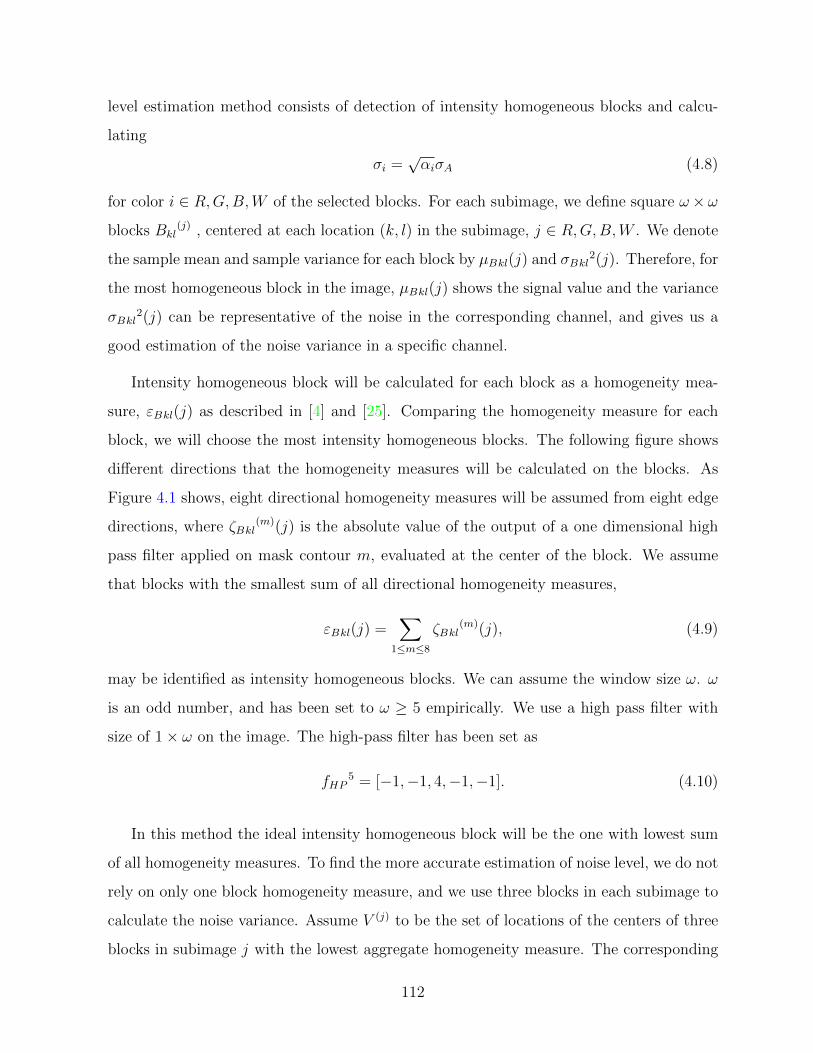
level estimation method consists of detection of intensity homogeneous blocks and calcu-

lating

σi =√αiσA (4.8)

for color i ∈ R,G,B,W of the selected blocks. For each subimage, we define square ω× ω

blocks Bkl(j) , centered at each location (k, l) in the subimage, j ∈ R,G,B,W . We denote

the sample mean and sample variance for each block by µBkl(j) and σBkl2(j). Therefore, for

the most homogeneous block in the image, µBkl(j) shows the signal value and the variance

σBkl2(j) can be representative of the noise in the corresponding channel, and gives us a

good estimation of the noise variance in a specific channel.

Intensity homogeneous block will be calculated for each block as a homogeneity mea-

sure, εBkl(j) as described in [4] and [25]. Comparing the homogeneity measure for each

block, we will choose the most intensity homogeneous blocks. The following figure shows

different directions that the homogeneity measures will be calculated on the blocks. As

Figure 4.1 shows, eight directional homogeneity measures will be assumed from eight edge

directions, where ζBkl(m)(j) is the absolute value of the output of a one dimensional high

pass filter applied on mask contour m, evaluated at the center of the block. We assume

that blocks with the smallest sum of all directional homogeneity measures,

εBkl(j) =∑

1≤m≤8

ζBkl(m)(j), (4.9)

may be identified as intensity homogeneous blocks. We can assume the window size ω. ω

is an odd number, and has been set to ω ≥ 5 empirically. We use a high pass filter with

size of 1× ω on the image. The high-pass filter has been set as

fHP5 = [−1,−1, 4,−1,−1]. (4.10)

In this method the ideal intensity homogeneous block will be the one with lowest sum

of all homogeneity measures. To find the more accurate estimation of noise level, we do not

rely on only one block homogeneity measure, and we use three blocks in each subimage to

calculate the noise variance. Assume V (j) to be the set of locations of the centers of three

blocks in subimage j with the lowest aggregate homogeneity measure. The corresponding

112

Figure 4.1: Eight different masks for homogeneity measures with the size ω = 5

sample variances are σBkl2(j), (k, l) ∈ V (j) for j ∈ R,G,B,W , and the estimate of the

variance for each phase is

σe,j2 =

1

3

∑(k,l)∈V (j)

σBkl2(j). (4.11)

If we know the exact ratio of αR : αG : αB : αW that was used to obtain fCFAN , we select

σeTα as,

σeTα = median[

σe,R√αR

,σe,G√αG

,σe,B√αB

,σe,W√αW

] (4.12)

where Tα stands for true alpha ratio, which means we apply the known alpha values for

estimating the noise standard deviation.

However, as we describe in Section 4.1, the ratio αR : αG : αB : αW can be different

depending on camera models. Therefore we may have to estimate the αR : αG : αB : αW

ratio first before we determine σe. From equation 4.6 we know

σR2 : σG

2 : σB2 : σW

2 = αR : αG : αB : αW , (4.13)

so we assumeσe,R√αR≈ σe,G√

αG≈ σe,B√

αB≈ σe,W√

αW. (4.14)

If we arbitrarily set αB = 1, then αR, αG and αW will be calculated.

The homogeneity in each block will be calculated using local uniformity analyzer, using

high-pass operators on a 5 × 5 mask in eight different directions. The results of the

113

local uniformity analyzer will be zero in the homogeneous area, and it is non-zero in non-

uniform areas. The sum of absolute values over the eight directions will be assumed as

the homogeneity factor. Using the homogeneity factor over the blocks, we find the average

variance of noise over the whole image.

Assuming there are 11 representative levels of noise, we will estimate the noise level of

input image, and select an appropriate set of filters to extract the color components and

demosaicking algorithm.

114

4.3 Demosaicking of noisy CFA images

The least-square demosaicking method has been proposed in Section 3.4 for RGBW

CFAs, and will be used for noise reduction. The noisy images will be used as a training

set for the least-square method. Different levels of Gaussian noise with parameter σ will

be added to the input CFA images. In the training phase, noise will be added to the

gamma-corrected R, G, B and W components with the given ratio of variances. The

standard deviation of noise for each color channel will be assumed as√αRσ,

√αGσ,

√αBσ

and√αWσ, and σ ∈ 0, 2, ..., 20 for eleven noise levels. Then, an appropriate least-square

demosaicking system will be designed for each set of noisy images. So we designed several

demosaicking systems, adapted to different levels of noise. In the proposed noise reduction

algorithm, the noise level of input image will be estimated, and an appropriate set of filters

for demosaicking will be chosen. The following block diagram 4.2 shows the demosaicking

and denoising algorithm.

Since the value of the estimated noise level is a continuous value and the added noise

level is a discrete value, we need to map the estimated value to one of the added noise

levels σ ∈ 0, 2, ..., 20, then the least square filter will be assigned. Assuming the noise level

2(p − 1), the color mean square error will be calculated and the best set of least square

filter σMS will be determined. We will select the nearest even noise level σdiscrete

σdiscrete = 2× round(σMS

2). (4.15)

The following plot Figure 4.3 shows the estimated noise variance versus the added noise

level over the 24 images of Kodak dataset using VEML sensor. The results illustrate that

the estimated noise level is close to the actual added noise value, and the appropriate least

square filter set has been chosen for each image.

115

Figure 4.2: Demosaicking-denoising system

116

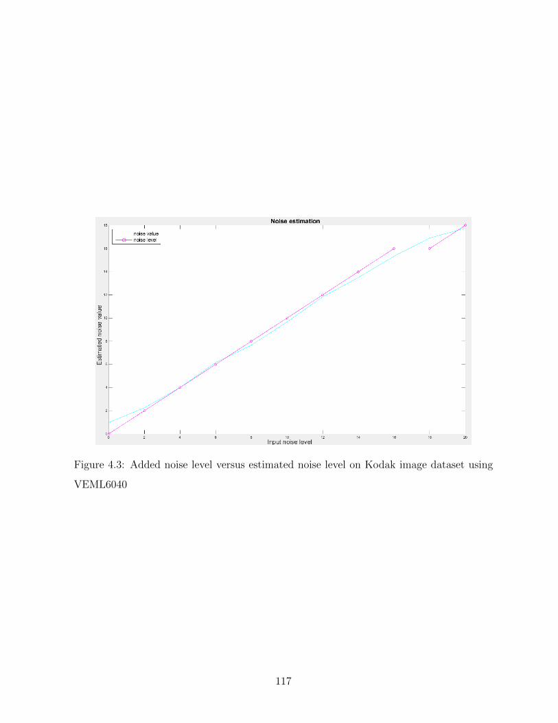
Figure 4.3: Added noise level versus estimated noise level on Kodak image dataset using

VEML6040

117

4.3.1 Luma noise reduction using BM3D

In the demosaicking algorithm, reconstructing the more accurate luma components is

crucial, and results in better quality of the reconstructed image. As we explained before,

during the demosaicking process the luma component will be calculated by subtracting

all chromas from the CFA. Since we are extracting chromas using noisy input images, the

estimated chromas will not be accurate, and it leads to the poor estimation of the luma

component. Using a state of art denoising method for gray scale images gives us a better

estimation of luma. We will apply the Block Matching 3D (BM3D) denoising algorithm

[12] in this stage, which is one of the state of the art denoising method.

4.4 Results

In this section, we designed and implemented the joint demosaicking-denoising algo-

rithm. As we discussed in this chapter, we added different levels of noise artificially to the

Kodak dataset. There will be ten different levels of white Gaussian noise with the variance

of σ = 0, 2, 4, ..., 20. Then the noise estimator will estimate the noise level and set the

suitable demosaicking algorithm for the estimated noise level to reconstruct the image.

The value of clear/panchromatic pixels have been estimated based on the equations

3.135 and 3.136 provided in Section 3.4.5 on the Kodak dataset. The results will be

compared with the hyperspectral image dataset with actual value of white pixels as well.

Tables 4.1, 4.2, 4.3 and 4.4 show the results of demosaicking-denoising method and

least-square method for Kodak dataset noisy images using RGBW-Bayer CFA in terms

of PSNR and S-CIELAB for VEML6040 and Kodak-KAI-11000 sensors. These tables

contain the average results over 24 images of Kodak data set in each case. The average

results over 24 images for different noise level show the proposed algorithm robustness in

different noise level, and let us compare the average results for RGBW-Bayer with the

average results of previous work for RGB-Bayer. According to the provided results in

the following tables the demosaicking-denoising algorithm is working better than regular

demosaicking algorithm without noise reduction method. A comparison between the state

118

of the art joint denoising-demosaicking method applied on RGB-Bayer is provided as well.

The denoising-demosaicking method on RGB-Bayer is working better than previous works

on this topic as discussed in [25].

Tables 4.1 and 4.3 show the results of regular least-square demosaicking method using

RGB-Bayer and RGBW-Bayer for Kodak dataset noisy images for both sensors. The

average PSNR of demosaicking-denoising method over 11 noise levels using RGBW-Bayer

is higher than the average PSNR using RGB-Bayer for both sensors. It shows that the

RGBW-Bayer pattern containing clear/ panchromatic filter receives higher signal to noise

ratio, and works better in presence of noise. We can conclude the same result based on

the S-CIELAB results as shown in Tables 4.2 and 4.4.

119

Noise level

(Noise variance)

LS method on

RGBW

LS method on

RGB

Demosaicking-

denoising on

RGBW

Demosaicking-

denoising on

RGB

1(0) 39.69 40.22 39.08 40.26

2(2) 37.77 37.96 37.59 37.51

3(4) 34.75 34.68 35.46 34.91

4(6) 32.18 32.00 34.11 32.90

5(8) 30.08 29.85 32.95 31.41

6(10) 28.35 28.10 32.03 30.27

7(12) 26.88 26.64 31.11 29.37

8(14) 25.62 25.38 30.26 28.69

9(16) 24.51 24.28 29.56 28.03

10(18) 23.52 23.31 28.96 27.51

11(20) 22.63 22.44 28.38 27.06

Average over 11

noise levels

29.63 29.53 32.68 31.62

Table 4.1: Average PSNR over 24 Kodak images using least-Square (LS) method and

demosaicking-denoising method on RGBW-Bayer using VEML6040 sensor and RGB-Bayer

for different noise levels

.

120

Noise level (Noise

variance)

LS method on RGBW Demosaicking-denoising on

RGBW

1(0) 0.85 1.01

2(2) 1.14 1.24

3(4) 1.65 1.62

4(6) 2.21 2.00

5(8) 2.81 2.38

6(10) 3.43 2.76

7(12) 4.05 3.16

8(14) 4.69 3.56

9(16) 5.33 3.95

10(18) 5.97 4.33

11(20) 6.62 4.72

Average over 11 noise

levels

3.52 2.79

Table 4.2: Average S-CIELAB over 24 Kodak images using least-Square(LS) method and

demosaicking-denoising method on RGBW-Bayer using VEML6040 sensor for different

noise levels

.

121

Noise level

(Noise variance)

LS method on

RGBW

LS method on

RGB

Demosaicking-

denoising on

RGBW

Demosaicking-

denoising on

RGB

1(0) 39.39 40.22 38.87 40.26

2(2) 37.14 37.96 36.89 37.51

3(4) 33.86 34.68 34.60 34.91

4(6) 31.17 32.00 33.55 32.90

5(8) 29.01 29.85 32.44 31.41

6(10) 27.25 28.10 31.17 30.27

7(12) 25.76 26.64 30.39 29.37

8(14) 24.49 25.38 29.50 28.69

9(16) 23.37 24.28 28.36 28.03

10(18) 22.38 23.31 27.92 27.51

11(20) 21.48 22.44 27.37 27.06

Average over 11

noise levels

28.66 29.53 31.91 31.62

Table 4.3: Average PSNR over 24 Kodak images using least-Square(LS) method and

demosaicking-denoising method on RGBW-Bayer using Kodak-KAI-11000 sensor and

RGB-Bayer for different noise levels

.

122

Noise level (Noise

variance)

LS method on RGBW Demosaicking-denoising on

RGBW

1(0) 0.95 1.11

2(2) 1.30 1.41

3(4) 1.89 1.87

4(6) 2.57 2.24

5(8) 3.27 2.66

6(10) 3.99 3.16

7(12) 4.73 3.58

8(14) 5.47 4.04

9(16) 6.22 4.52

10(18) 6.98 4.93

11(20) 7.74 5.39

Average over 11 noise

levels

4.10 3.17

Table 4.4: Average S-CIELAB over 24 Kodak images using least-Square(LS) method and

demosaicking-denoising method on RGBW-Bayer using Kodak-KAI-11000 sensor for dif-

ferent noise levels

.

123

The following figures show the noisy CFA images for two sample images and two dif-

ferent noise levels in each case (σ = 6, 14), as well as the reconstructed image using least-

square demosaicking method (presented in previous chapter) and demosaicking-denoising

algorithm. As we can see visually in Figures 4.4 and 4.5, the quality of reconstructed im-

ages using demosaicking-denoising algorithm are better than the quality of reconstructed

images using LS method in different input noise levels. The CFA images are not meant

to be displayed, and they do not have a good quality. We present them here to show the

effect of noise in different noise level in the CFA images.

124

(a) Original Image

(b) Noisy CFA

Image with noise

level=4

(c) Reconstructed

using LS method

(d) Reconstructed

using demosaicking-

denoising method

(e) Original Image

(f) Noisy CFA

Image with noise

level=4

(g) Reconstructed

using LS method

(h) Reconstructed

using demosaicking-

denoising method

Figure 4.4: Reconstructed noisy image with σ = 6 using regular least-square demosaicking

method and denoising-demosaicking method with RGBW-Bayer CFA

125

(a) Original Image

(b) Noisy CFA

Image with noise

level=8

(c) Reconstructed

using LS method

(d) Reconstructed

using demosaicking-

denoising method

(e) Original Image

(f) Noisy CFA

Image with noise

level=8

(g) Reconstructed

using LS method

(h) Reconstructed

using demosaicking-

denoising method

Figure 4.5: Reconstructed noisy image with σ = 14 using regular least-square demosaicking

method and denoising-demosaicking method with RGBW-Bayer CFA

126

All the provided results above have been simulated and tested on RGB Kodak data

set. The following tables show the result of demosaicking-denoising algorithm with least-

square method on a hyperspectral dataset [33] for both sensors. The RGB and RGBW

images have been calculated based on the hyperspectral images, and the RGB and RGBW

CFAs have been reconstructed for each image. Therefore, we are simulating the actual

captured white values from the clear/panchromatic filters using hyperspectral images and

we are comparing the results with reconstructed images using the RGB-Bayer on the same

dataset.

Tables 4.5 and 4.6 provide the average PSNR over the 30 images of dataset for both

sensors. The noisy RGBW CFA have been reconstructed by adding different noise level to

the CFA image, as we discussed before. Using the average results over 30 hyperspectral

images for different noise level we will be able to compare the proposed algorithm robustness

in different noise level, and let us compare the average results for RGBW-Bayer with the

average results of Kodak dataset for RGBW-Bayer.

Since we are using two different datasets, we will not be able to compare the average

PSNR over the whole dataset with the previous results. The provided results are showing

that the proposed demosaicking-denoising algorithm is working very well on hyperspectral

images as a sample of received image with RGBW CFAs in presence of noise.

It shows that the demosaicking-denoising algorithm is working better than regular

demosaicking algorithm without noise reduction method. A comparison between the state

of art joint denoising-demosaicking method applied on RGBW-Bayer on Kodak dataset is

provided as well. The results shows that the RGBW CFA is more robust to noise than the

RGB CFA as we hypothesized in this research.

127

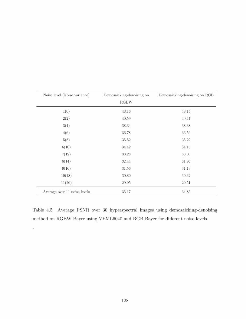
Noise level (Noise variance) Demosaicking-denoising on

RGBW

Demosaicking-denoising on RGB

1(0) 43.16 43.15

2(2) 40.59 40.47

3(4) 38.34 38.38

4(6) 36.78 36.56

5(8) 35.52 35.22

6(10) 34.42 34.15

7(12) 33.28 33.00

8(14) 32.44 31.96

9(16) 31.56 31.13

10(18) 30.80 30.32

11(20) 29.95 29.51

Average over 11 noise levels 35.17 34.85

Table 4.5: Average PSNR over 30 hyperspectral images using demosaicking-denoising

method on RGBW-Bayer using VEML6040 and RGB-Bayer for different noise levels

.

128

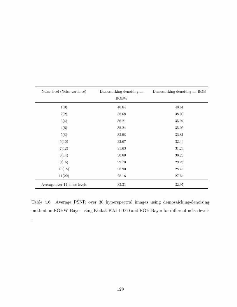
Noise level (Noise variance) Demosaicking-denoising on

RGBW

Demosaicking-denoising on RGB

1(0) 40.64 40.61

2(2) 38.68 38.03

3(4) 36.21 35.94

4(6) 35.24 35.05

5(8) 33.98 33.81

6(10) 32.67 32.43

7(12) 31.63 31.23

8(14) 30.60 30.23

9(16) 29.70 29.28

10(18) 28.90 28.43

11(20) 28.16 27.64

Average over 11 noise levels 33.31 32.97

Table 4.6: Average PSNR over 30 hyperspectral images using demosaicking-denoising

method on RGBW-Bayer using Kodak-KAI-11000 and RGB-Bayer for different noise levels

.

129

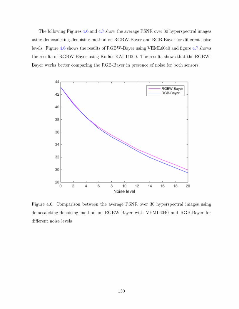
The following Figures 4.6 and 4.7 show the average PSNR over 30 hyperspectral images

using demosaicking-denoising method on RGBW-Bayer and RGB-Bayer for different noise

levels. Figure 4.6 shows the results of RGBW-Bayer using VEML6040 and figure 4.7 shows

the results of RGBW-Bayer using Kodak-KAI-11000. The results shows that the RGBW-

Bayer works better comparing the RGB-Bayer in presence of noise for both sensors.

Figure 4.6: Comparison between the average PSNR over 30 hyperspectral images using

demosaicking-denoising method on RGBW-Bayer with VEML6040 and RGB-Bayer for

different noise levels

130

Figure 4.7: Comparison between the average PSNR over 30 hyperspectral images using

demosaicking-denoising method on RGBW-Bayer with Kodak-KAI11000 and RGB-Bayer

for different noise levels

131

Also, the following tables 4.7, 4.8 show the average S-CIELAB results of 30 hyper-

spectral images using demosaicking-denoising method on RGBW-Bayer and RGB-Bayer

for different noise levels for both sensors. The average SCIELAB show the similarity be-

tween the original image and the reconstructed image in presence of noise using denoising-

demosaicking algorithm over the whole data set for each noise level. The comparison

between RGB-Bayer and RGBW-Bayer shows that the RGBW-Bayer is working better for

noisy input images.

Noise level (Noise variance) Demosaicking-denoising on

RGBW

Demosaicking-denoising on RGB

1(0) 0.53 0.46

2(2) 0.84 0.85

3(4) 1.25 1.27

4(6) 1.66 1.66

5(8) 2.08 2.12

6(10) 2.50 2.58

7(12) 2.93 3.02

8(14) 3.35 3.50

9(16) 3.78 3.92

10(18) 4.20 4.37

11(20) 4.64 4.82

Average over 11 noise levels 2.52 2.59

Table 4.7: Average S-CIELAB over 30 hyperspectral images using demosaicking-denoising

method on RGBW-Bayer using VEML6040 and RGB-Bayer for different noise levels

.

132

Noise level (Noise variance) Demosaicking-denoising on

RGBW

Demosaicking-denoising on RGB

1(0) 0.66 0.64

2(2) 1.063 1.07

3(4) 1.58 1.65

4(6) 2.08 2.17

5(8) 2.60 2.66

6(10) 3.13 3.26

7(12) 3.66 3.76

8(14) 4.20 4.27

9(16) 4.74 4.79

10(18) 5.27 5.35

11(20) 5.80 5.83

Average over 11 noise levels 3.16 3.22

Table 4.8: Average S-CIELAB over 30 hyperspectral images using demosaicking-denoising

method on RGBW-Bayer using Kodak-KAI-11000 and RGB-Bayer for different noise levels

.

133

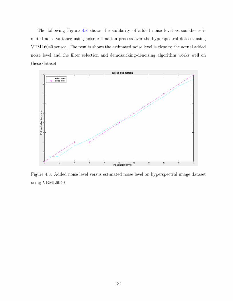
The following Figure 4.8 shows the similarity of added noise level versus the esti-

mated noise variance using noise estimation process over the hyperspectral dataset using

VEML6040 sensor. The results shows the estimated noise level is close to the actual added

noise level and the filter selection and demosaicking-denoising algorithm works well on

these dataset.

Figure 4.8: Added noise level versus estimated noise level on hyperspectral image dataset

using VEML6040

134

Chapter 5

Conclusion

5.1 Conclusions

A novel demosaicking-denoising method for RGBW CFAs has been introduced in this

research. According to the results, the presented method led to a noticeable improvement

in received signal to noise ratio compared to the existing methods in the literature. The

presented methods included a demosaicking algorithm on a three channel CFA and three

four channel CFAs. The contributions were as follows:

• Due to the complexity of the Fujifilm X-Trans pattern, it has been chosen to study

among three-channel CFAs, and adaptive and non-adaptive and least-square demo-

saicking algorithms have been developed for it. Since there is no available literature

on Fujifilm X-Trans pattern demosaicking, the results have been compared with the

state of the art demosaicking method on RGB-Bayer. The Fujifilm X-Trans pattern

has a large number of color filters, and it provides more accurate color estimation

through demosaicking process, but it is not work as good as Bayer pattern in high

frequency areas. The results have been presented at the International Conference of

Image Processing (ICIP)-2014 [38].

• The RGBW-Kodak pattern has been modeled, and adaptive and non-adaptive demo-

saicking algorithms have been proposed for it. It has been published in SPIE/ IS&T

135

Electronic Imaging-2015 conference [39]. Also, a recently developed RGBW pattern

presented in [45] has been reviewed in this work and a demosaicking algorithm has

been implemented for this pattern. The RGBW-Bayer CFA has been discussed,

and adaptive and non-adaptive demosaicking algorithms have been presented for it.

Also the adaptive demosaicking algorithm for three-channel and four-channel CFAs

has been presented in a structured and organized method, and it can be applied on

different CFAs.

In our initial assumption, we simulate the white filters output as a combination

of red, green and blue filters. The best estimation of white filter output has been

calculated using the other three primary color components by quadratic program-

ming. The adaptive demosaicking algorithm for RGBW-Bayer has been optimized

using least-squares method. The comparison between different RGBW patterns has

been presented in this research, and it has been published in SPIE/ IS&T Electronic

Imaging-2016 conference [40].

Initially, the Kodak data set has been used for comparing the results. The results

shows less color artifacts for Fujifilm X-Trans pattern compared to the RGB-Bayer.

The results of demosaicking algorithms for all three RGBW patterns have been com-

pared. The visual results and the PSNR show that RGBW-Bayer was the best among

the discussed patterns. The least-square method results for RGBW-Bayer have been

compared with the least-square method using RGB-Bayer pattern.

• The effect of noise has been simulated on red, green, blue and white filters, and an ap-

propriate demosaicking-denoising algorithm on RGBW-Bayer pattern has been devel-

oped using a new set of coefficients for noise in different channel. The demosaicking-

denoising algorithm results on Bayer-RGBW CFA with demosaicking-denoising algo-

rithm on RGB-Bayer results have been compared. Thus the results of noise reduction

on white color filters has been evaluated. The proposed algorithm has been applied on

Kodak dataset and a hyperspectral dataset. Also the white filter estimation results

have been validated using hyperspectral images. The results have been white bal-

anced and gamma corrected, and the SCIELAB and PSNR values for each developed

136

demosaicking algorithm have been measured.

The results of four channel CFA have been evaluated on a hyperspectral data set [33]

as well. The results of demosaicking-denoising algorithm using both hyperspectral

and Kodak images shows improvement using RGBW-Bayer CFA comparing to the

RGB-Bayer CFA. The comparison between the white filter estimation using the opti-

mized equation 3.135 based on the value of three primary color filters (red,green and

blue) and the actual white filter values of hyperspectral images shows the estimated

values are very accurate.

5.2 Future work

The proposed algorithms for RGB and RGBW color filter arrays led to a new demosaicking-

denoising algorithm for RGBW CFAs. The results of this research can be expanded to

different aspects. Some suggested future works are as follows:

• As this research showed the signal to noise ratio has higher value using RGBW

CFAs, studying and creating CFAs containing more white filters can improve the

reconstructed image quality.

• A case study is applying the presented adaptive, non-adaptive, and least-square de-

mosaicking method, on different CFAs. Since, there might be a better RGBW CFA

to reconstruct the color images, the proposed demosaicking-denoising algorithm can

be applied on other RGBW CFAs.

• The modeled white filter based on red, green and blue filters value, can be utilized

to replace color filters with white filters. Designing new CFA patterns with two color

filters and more white filters can be another research direction in future.

137

References

[1] J. E. Adams. Design of practical color filter array interpolation algorithms for digital

cameras. IEEE International Conference On Image Processing (ICIP), 1(8):518–533,

1998.

[2] J. E. Adams, A. Deever, J. F. Hamilton Jr, M. Kumar, R. Palum, and B. H. Pillman.

Single capture image fusion with motion consideration. In Rastislav Lukac, editor,

Computational Photography: Methods and Applications, chapter 2, page 63. CRC

Press, 2010.

[3] D. Alleysson, S. Susstrunk, and J. Herault. Linear demosaicing inspired by the human

visual system. IEEE transaction on Image Processing, 14(4), 2005.

[4] A. Amer and E. Dubois. Fast and reliable structure-oriented video noise estimation.

IEEE Transactions on Circuits and Systems for Video Technology, 15(1):113–118,

2005.

[5] A. Buades, Y. Lou, J. Morel, and Z. Tang. Multi image noise estimation

and denoising. https://hal.archives-ouvertes.fr/hal-00510866/file/BurstHal.pdf, (hal−

00510866), 2010.

[6] H. C. Burger, C. J. Schuler, and S. Harmeling. Image denoising: Can plain neural

networks compete with BM3D. In IEEE Conference on Computer Vision and Pattern

Recognition (CVPR), pages 2392–2399, 2012.

[7] P. Chatterjee, N. Joshi, Sing Bing Kang, and Y. Matsushita. Noise suppression in

low-light images through joint denoising and demosaicing. In IEEE Conference on

138

Computer Vision and Pattern Recognition, CVPR ’11, pages 321–328. IEEE Computer

Society, 2011.

[8] D. R. Cok. Signal processing method and apparatus for producing interpolated chromi-

nance values in a sampled color image signal. U.S. Patent No. 4 642 678, 1987.

[9] Eastman Kodak Company. Kodak, KAI-11002 image sensor.[online]. website:. https:

//www.pco.de/fileadmin/user_upload/db/download/KAI-11000CMLongSpec.pdf,

2006.

[10] Vishay Company. VEML Sensor-Vishay.[online]. website:. http://www.vishay.com/

docs/84276/veml6040.pdf.

[11] S. Courroux, S. Guyetant, S. Chevobbe, and M. Paindavoine. A wavelet-based demo-

saicking algorithm for embedded applications. In Conference on Design and Architec-

tures for Signal and Image Processing (DASIP), 2010.

[12] K. Dabov, A. Foi, V. Katkovnik, and K. Egiazarian. Image denoising by sparse 3-D

transform-domain collaborative filtering. IEEE Transactions on Image Processing,

16(8):2080–2095, 2007.

[13] W. Dong, X. Li, L. Zhang, and G. Shi. Sparsity-based image denoising via dictionary

learning and structural clustering. In IEEE Conference on Computer Vision and

Pattern Recognition (CVPR), pages 457–464, 2011.

[14] J. Driesen and P. Scheunders. Wavelet-based color filter array demosaicking. In IEEE

International Conference on Image Processing (ICIP), volume 5, 2004.

[15] E. Dubois. Lslcd algorithm performance on different sampling structures.[online]. web-

site:. http://www.site.uottawa.ca/~edubois/SingleSensorImaging/Structure_

comparison/.

[16] E. Dubois. Frequency-domain methods for demosaicking of Bayer-sampled color im-

ages. IEEE Signal Processing Letters, 12(12):847, 2005.

139

[17] E. Dubois. The Structure and Properties of Color Spaces and the Representation of

Color Images. Morgan & Claypool Publishers, 1st edition, 2009.

[18] E.Dubois. Color filter array sampling of color images: Frequency-domain analysis and

associated demosaicking algorithms. In Rastislav Lukac, editor, Single-Sensor Imaging

Methods and Applications for Digital Cameras, chapter 7, pages 183–212. CRC Press,

2008.

[19] Fujifilm. FUJIFILM X-Pro1. [online]. website:. http://www.fujifilmusa.com/

products/digital-cameras/x/fujifilm-x-pro1/features.

[20] B. K. Gunturk, Y. Altunbasak, and R. M. Mersereau. Color plane interpolation using

alternating projections. IEEE transaction on Image Processing, 11(9):997–1013, 2002.

[21] B. K. Gunturk, J. Glotzbach, Y. Altunbasak, R. W. Schafer, and R. M. Mersereau.

Demosaicking: color filter array interpolation. IEEE Signal Processing Magazine,

22(1):44–54, Jan 2005.

[22] J.F. Hamilton and J.T. Compton. Processing color and panchromatic pixels. U.S.

Patent No.: US8274715B2, 2012.

[23] K. Hirakawa and T. W. Parks. Adaptive homogeneity-directed demosaicing algorithm.

IEEE transaction on Image Processing, 14(3), 2005.

[24] M. Hirakawa, K. Xiao-Li and P. J. Wolfe. A framework for wavelet-based analysis

and processing of color filter array images with applications to denoising and demo-

saicing. In IEEE International Conference on Acoustics, Speech and Signal Processing

(ICASSP), volume 1, 2007.

[25] G. Jeon and E. Dubois. Demosaicking of noisy Bayer-sampled color images with least-

squares luma-chroma demultiplexing and noise level estimation. IEEE Transactions

on Image Processing,, 22(1):146–156, 2013.

[26] G. M. Johnson and M. D. Fairchild. A top down description of S-CIELAB and

ciede2000. Color Research Application, 28(6):425–435, 2003.

140

[27] R. W. B. Kolta, H. A. Aly, and W. Fakhr. A hybrid demosaicking algorithm us-

ing frequency domain and wavelet methods. In International Conference on Image

Information Processing (ICIIP), 2011.

[28] B. Leung, G. Jeon, and E. Dubois. Demosaicking of noisy Bayer-sampled color im-

ages with Least-Squares luma-chroma demultiplexing and noise level estimation: Ad-

ditional results.[online]. website:. http://www.site.uottawa.ca/~edubois/lslcd/.

[29] B. Leung, G. Jeon, and E. Dubois. Least-squares luma chroma demultiplexing algo-

rithm for Bayer demosaicking. IEEE Transactions on Image Processing, 20(7):1885–

1894, 2011.

[30] X. Li, B. K. Gunturk, and L. Zhang. Image demosaicing: A systematic survey. Inter-

national Society for Optics and Photonics, pages 68221J–68221J, 2008.

[31] R. Lukac and K. N. Plataniotis. Single-sensor camera image processing. In Rastislav

Lukac, editor, Color image processing: methods and applications, chapter 16, pages

363–392. CRC press, 2006.

[32] D. Menon and G. Calvagno. Color image demosaicking: an overview. Signal Process-

ing: Image Communication, 26(8):518–533, 2011.

[33] F. Moghareh Abed. Pigment identification of paintings based on Kubelka-Munk theory

and spectral images. PhD Thesis. Rochester Institute of Technology, 2014.

[34] T. K. Moon and W. C. Stirling. Mathematical methods and algorithms for signal

processing. Prentice Hall, Upper Saddle River, NJ, 2000.

[35] M. Nawrath and J. Jakel. Deriving color images from noisy Bayer data using local

demosaicking and non-local denoising. In International Conference on Image and

Signal Processing (CISP), volume 2, pages 668–672, 2011.

[36] R. Niruban, T. Sree Renga Raja, and T. Sree Sharmila. Novel color filter array demo-

saicing in frequency domain with spectral refinement. Jurnal of Computer Science,

10:1591–1599, 2014.

141

[37] Ch. Poynton. Macbeth Color Checker.[online]. website:. http://www.poynton.com/

notes/color/GretagMacbeth-ColorChecker.html.

[38] M. Rafinazari and E. Dubois. Demosaicking algorithm for the fujifilm X-Trans color

filter array. In IEEE International Conference on Image Processing (ICIP), 2014.

[39] M. Rafinazari and E. Dubois. Demosaicking algorithm for the Kodak-RGBW color

filter array. in Proc. Color Imaging XXI: Displaying, Processing, Hardcopy, and Ap-

plications,Electronic Imaging-SPIE, 9395, 2015.

[40] M. Rafinazari and E. Dubois. Demosaicking algorithms for different RGBW color

filter arrays. in Proc. Color Imaging XXI: Displaying, Processing, Hardcopy, and

Applications,Electronic Imaging-SPIE, 9395:COLOR–312.1–6, 2016.

[41] S. Sari, H. Roslan, and T. Shimamura. Noise estimation by utilizing mean devia-

tion of smooth region in noisy image. International Conference on Computational

Intelligence, Modelling and Simulation, 2012.

[42] Sony. Sony-RGBE. [online]. website:. http://www.dpreview.com/articles/

1471104084/sonyrgbeccd.

[43] H. P. Sung, S. K. Hyung, S. Lansel, M. Parmar, and B. A. Wandell. A case for

denoising before demosaicking color filter array data. In Asilomar Conference on

Signals, Systems and Computers, pages 860–864, Nov 2009.

[44] C. Tomasi and R. Manduchi. Bilateral filtering for gray and color images. International

Conference on Computer Vision, 1998.

[45] J. Wang, Ch. Zhang, and P. Hao. New color filter arrays of high light sensitivity and

high demosaicking performance. IEEE International Conference on Image Processing

(ICIP), pages 3153–3156, 2011.

142