density-based shape descriptors and ... - cmpe · pdf file4.7 basic score usionf ... 4.10.1...
TRANSCRIPT

DENSITY-BASED SHAPE DESCRIPTORS
AND SIMILARITY LEARNING
FOR 3D OBJECT RETRIEVAL
Ceyhun Burak Akgül
submitted to
Ecole Nationale Supérieure des Télécommunications, Paris
&
Bo§aziçi University, Istanbul
in partial fulllment of the requirements
for the degree of
Doctor of Philosophy
December 2007

2

"Naturally, the four mathematical operations -adding, subtracting, multiplying, and dividing -were impossible. The stones resisted arithmeticas they did the calculation of probability. Fortydisks, divided, might become nine; those ninein turn divided might yield three hundred."
Jorge Luis Borges Blue Tigers
3

4

Acknowledgements
I am very grateful to my two thesis supervisors, Bülent Sankur and Francis Schmitt,and my co-supervisor Yücel Yemez for all they brought to this work, for expressing theircritical minds on every occasion, and especially for being the devil's advocate. I've heardthis expression for the rst time from Bülent Sankur, now a long time ago. So you canimagine how much I was surprised when I heard it again from Francis Schmitt at my arrivalto ENST1. This was an indication for the things to come, an indication for the "future"which is now the "past" that I will never regret. The diculty and the joy of making athesis in two institutions is to satisfy more than one person with his work, but also to protfrom more than one exceptional mind to perfect it. I had this very chance of working withthese three people who have shown me dierent dimensions of pursuing a doctoral thesis.In particular, I would like to thank Francis Schmitt for introducing me into the fascinating3D domain and for sharing his vast knowledge with me ; I would like to thank Yücel Yemezfor always indicating the good pointers and also for our discussions during the toughestmoments.
I would like to express my gratitude to Bülent Sankur for discovering the researcherthat I am, for all I've learned from him, for his trust in me... There is a very long list ofthings for which I have to express my gratitude. I hope he knows how much I am grateful.
I would like to thank Nozha Boujemaa for accepting the presidency of the jury. Iwould like to thank Ethem Alpaydn and Atilla Ba³kurt for being thesis reporters and jurymembers especially with many constraints concerning time and travel. Their appreciationfor my work encourages me to continue in research. And also... Note the date of the thesisdefense : it's 19th December 2007. That day, the metro wasn't working properly in Paris,and it was extremely hard to nd a taxi. The jury members made their own way to be ontime in the morning, even if they had to walk in Paris streets. I would like to thank all thejury members for this too.
I would like to thank Isabelle Bloch for her comments on the thesis presentation just aweek before the defense. Her remarks had wonderful eects on the great day. I would liketo thank Burak Acar for being a member of the thesis follow-up committee. I would liketo thank Selim Eskiizmirliler for his support as a genuine Galatasaray brother.
I would like to thank Jérôme Darbon, exceptional researcher and "Roi de la Butte-aux-Cailles", Georoy Fouquier "Le Duc" and David Lesage "L'Aventurier" for their friendshipand unconditional support. From Bo§aziçi side, I would like to thank Helin Duta§ac andErdem Yörük : these two people have always helped me without knowing and withoutexpecting anything. In particular, I would like to thank Helin Duta§ac for this fantasticjob of generating an expert classication for the Sculpteur database.
1This work has been done in two research labs ENST/TSI and BUSIM (Bo§aziçi University) in theframework of the joint doctoral thesis programme between ENST and Bo§aziçi University. A part of mystudies in France has been funded by CROUS de Paris.
5

Again the joy of making a thesis in two institutions is to double the number of mateson this way that we call "to make a thesis". I would like to thank Tony Tung et CarlosHernández-Esteban : I made a lot use of the tools they've developed during the Sculpteurproject. Without discriminating between generations, I would like to thank all the peoplethat I've known at TSI and at BUSIM. In particular, my sincere thanks to Jérémie, Julien,Eve, Alex, Gero, Antonio, Camille, Olivier, Ebru, pek, Ça§atay and Oya. I had very nicemoments with them. I would like to thank also Sophie-Charlotte, Najib and Saïd withwhom I shared many coe breaks ; Soane, my last oce mate and the postdocs Sylvieand Vincent.
I would like to thank all my friends for their appreciation and the courage they gave meduring all the way towards the end. In particular, I am grateful to Fulden, Eren, Funda andBa³ak for being there on this great day and night ! Fulden and Eren had non-professsionalremarks on the presentation, that I used a lot during the defense. Even they didn't know,in their eyes I found the courage that I needed.
I would like to thank Fulden, not only being present in the thesis defense, but especiallybeing there since the beginning of the world and time.
Finally, a thousand thanks to my mother Emel, my father Ne³at and my sister Ay³egül.To defend a thesis, I needed their constant support they gave me very generously andwithout fatigue. There is no word to express my gratitude to them. I hope this thesisshows that their supports and sacrices weren't in vain.
6

Abstract
Next generation search engines will enable query formulations, other than text, relyingon visual information encoded in terms of images and shapes. The 3D search technology,in particular, targets specialized application domains ranging from computer aided-designand manufacturing to cultural heritage archival and presentation. Content-based retrievalresearch aims at developing search engines that would allow users to perform a query bysimilarity of content.
This thesis deals with two fundamentals problems in content-based 3D object retrieval:
(1) How to describe a 3D shape to obtain a reliable representative for the subsequenttask of similarity search?
(2) How to supervise the search process to learn inter-shape similarities for more eectiveand semantic retrieval?
Concerning the rst problem, we develop a novel 3D shape description scheme basedon probability density of multivariate local surface features. We constructively obtainlocal characterizations of 3D points on a 3D surface and then summarize the resultinglocal shape information into a global shape descriptor. For probability density estimation,we use the general purpose kernel density estimation methodology, coupled with a fastapproximation algorithm: the fast Gauss transform. The conversion mechanism from localfeatures to global description circumvents the correspondence problem between two shapesand proves to be robust and eective. Experiments that we have conducted on several 3Dobject databases show that density-based descriptors are very fast to compute and veryeective for 3D similarity search.
Concerning the second problem, we propose a similarity learning scheme that incor-porates a certain amount of supervision into the querying process to allow more eectiveand semantic retrieval. Our approach relies on combining multiple similarity scores byoptimizing a convex regularized version of the empirical ranking risk criterion. This scorefusion approach to similarity learning is applicable to a variety of search engine problemsusing arbitrary data modalities. In this work, we demonstrate its eectiveness in 3D objectretrieval.
7

8

Contents
Introduction 13
1 3D Object Retrieval 17
1.1 Research Challenges in 3D Object Retrieval . . . . . . . . . . . . . . . . . . 171.2 3D Object Databases . . . . . . . . . . . . . . . . . . . . . . . . . . . . . . . 201.3 Background on 3D Shape Descriptors . . . . . . . . . . . . . . . . . . . . . . 24
1.3.1 Histogram-Based Methods . . . . . . . . . . . . . . . . . . . . . . . . 251.3.2 Transform-Based Methods . . . . . . . . . . . . . . . . . . . . . . . . 271.3.3 Graph-Based Methods . . . . . . . . . . . . . . . . . . . . . . . . . . 28
1.4 Similarity Measures . . . . . . . . . . . . . . . . . . . . . . . . . . . . . . . . 291.5 Evaluation Tools for Retrieval . . . . . . . . . . . . . . . . . . . . . . . . . . 30
2 Density-Based 3D Shape Description 33
2.1 Local Characterization of a 3D Surface . . . . . . . . . . . . . . . . . . . . . 342.1.1 Local Surface Features . . . . . . . . . . . . . . . . . . . . . . . . . . 342.1.2 Feature Calculation . . . . . . . . . . . . . . . . . . . . . . . . . . . 392.1.3 Target Selection . . . . . . . . . . . . . . . . . . . . . . . . . . . . . 40
2.2 Kernel Density Estimation . . . . . . . . . . . . . . . . . . . . . . . . . . . . 432.2.1 KDE in Context . . . . . . . . . . . . . . . . . . . . . . . . . . . . . 442.2.2 Bandwidth Selection . . . . . . . . . . . . . . . . . . . . . . . . . . . 472.2.3 Computational Considerations . . . . . . . . . . . . . . . . . . . . . 51
2.3 Descriptor Manipulation Tools . . . . . . . . . . . . . . . . . . . . . . . . . 522.3.1 Marginalization . . . . . . . . . . . . . . . . . . . . . . . . . . . . . . 522.3.2 Probability Density Pruning . . . . . . . . . . . . . . . . . . . . . . . 53
2.4 An Invariant Similarity Measure for Pdfs . . . . . . . . . . . . . . . . . . . . 542.5 Summary of the Algorithm . . . . . . . . . . . . . . . . . . . . . . . . . . . 57
3 Statistical Similarity Learning 59
3.1 The Score Fusion Problem . . . . . . . . . . . . . . . . . . . . . . . . . . . . 613.2 Ranking Risk Minimization . . . . . . . . . . . . . . . . . . . . . . . . . . . 623.3 SVM Formulation . . . . . . . . . . . . . . . . . . . . . . . . . . . . . . . . . 623.4 Applications . . . . . . . . . . . . . . . . . . . . . . . . . . . . . . . . . . . . 64
3.4.1 Bimodal Search . . . . . . . . . . . . . . . . . . . . . . . . . . . . . . 643.4.2 Two-round Search . . . . . . . . . . . . . . . . . . . . . . . . . . . . 65
9

CONTENTS
4 Experiments 67
4.1 Bandwidth Selection . . . . . . . . . . . . . . . . . . . . . . . . . . . . . . . 694.1.1 Levels of Analysis for Bandwidth Selection . . . . . . . . . . . . . . . 694.1.2 Sensitivity Results . . . . . . . . . . . . . . . . . . . . . . . . . . . . 69
4.2 Robustness Results . . . . . . . . . . . . . . . . . . . . . . . . . . . . . . . . 724.2.1 Eect of Feature Calculation . . . . . . . . . . . . . . . . . . . . . . 724.2.2 Robustness against Low Mesh Resolution . . . . . . . . . . . . . . . 724.2.3 Robustness against Noise . . . . . . . . . . . . . . . . . . . . . . . . 744.2.4 Robustness against Pose Normalization Errors . . . . . . . . . . . . . 75
4.3 Target Selection . . . . . . . . . . . . . . . . . . . . . . . . . . . . . . . . . . 764.3.1 Eect of Sampling Schemes . . . . . . . . . . . . . . . . . . . . . . . 764.3.2 Eect of Descriptor Size . . . . . . . . . . . . . . . . . . . . . . . . . 76
4.4 Similarity Measures . . . . . . . . . . . . . . . . . . . . . . . . . . . . . . . . 764.5 Dimensionality Reduction . . . . . . . . . . . . . . . . . . . . . . . . . . . . 78
4.5.1 Marginalization Results . . . . . . . . . . . . . . . . . . . . . . . . . 794.5.2 Probability Density Pruning Results . . . . . . . . . . . . . . . . . . 794.5.3 PCA Results . . . . . . . . . . . . . . . . . . . . . . . . . . . . . . . 79
4.6 Feature-Level Fusion . . . . . . . . . . . . . . . . . . . . . . . . . . . . . . . 814.6.1 A Few Examples . . . . . . . . . . . . . . . . . . . . . . . . . . . . . 814.6.2 Marginalization Revisited . . . . . . . . . . . . . . . . . . . . . . . . 84
4.7 Basic Score Fusion . . . . . . . . . . . . . . . . . . . . . . . . . . . . . . . . 854.8 Comparison to Other Methods . . . . . . . . . . . . . . . . . . . . . . . . . 88
4.8.1 Comparison with Histogram-Based Peers . . . . . . . . . . . . . . . . 884.8.2 General Comparison . . . . . . . . . . . . . . . . . . . . . . . . . . . 94
4.9 Performance Variation across Databases . . . . . . . . . . . . . . . . . . . . 974.10 Statistical Learning-Based Score Fusion . . . . . . . . . . . . . . . . . . . . 104
4.10.1 Performance in the Bimodal Search . . . . . . . . . . . . . . . . . . . 1064.10.2 Performance in the Two-round Search . . . . . . . . . . . . . . . . . 107
5 Conclusion and Perspectives 113
5.1 Discussion and Conclusion . . . . . . . . . . . . . . . . . . . . . . . . . . . . 1135.2 Perspectives . . . . . . . . . . . . . . . . . . . . . . . . . . . . . . . . . . . . 116
Notations 119
A 3D Object Databases 121
B Standard Dissimilarity Measures 125
B.1 Lp-Distances . . . . . . . . . . . . . . . . . . . . . . . . . . . . . . . . . . . 125B.2 Symmetric Kullback-Leibler Distance . . . . . . . . . . . . . . . . . . . . . . 126B.3 χ2-Divergence . . . . . . . . . . . . . . . . . . . . . . . . . . . . . . . . . . . 126B.4 Bhattacharyya Distance . . . . . . . . . . . . . . . . . . . . . . . . . . . . . 126B.5 Histogram Intersection . . . . . . . . . . . . . . . . . . . . . . . . . . . . . . 127B.6 Earth Mover's Distance . . . . . . . . . . . . . . . . . . . . . . . . . . . . . 127
C KDE and Related Issues 129
C.1 Derivation . . . . . . . . . . . . . . . . . . . . . . . . . . . . . . . . . . . . . 129C.2 Derivation of the Upper Bound on MIAE . . . . . . . . . . . . . . . . . . . 130C.3 AMISE and the Scott Bandwidth . . . . . . . . . . . . . . . . . . . . . . . . 132
10

CONTENTS
D Marginalization Results 135
E Sample Two-round Searches 139
F Publications 145
F.1 Publications Related to the Thesis . . . . . . . . . . . . . . . . . . . . . . . 145F.2 Other Publications in 2004-2007 . . . . . . . . . . . . . . . . . . . . . . . . . 146
Bibliography 147
11

12

Introduction
Communication media have appeared in many guises during the never ending InformationAge. The passage from textual exchange of ideas to audiovisual communication had beenone of the major breakthroughs in the last century. Visual information in the form of imageand video has now become so common that we cannot even imagine a world without photos,television and motion pictures. The advent of high-speed graphics hardware now oers anew dress to visual information: the digital 3D object.
3D objects arise in a number of disciplines ranging from computer aided-design andmanufacturing (CAD/CAM) to cultural heritage archival and presentation. Other shadesof the application spectrum include architecture, medicine, molecular biology, military,virtual reality and entertainment. Access to large 3D object databases occurring in theseelds demands eective and ecient tools for indexing, categorization, classication andrepresentation of the 3D data. Content-based retrieval addresses this challenging taskusing compact shape representations and intelligent search paradigms.
The next generation search engines will enable query formulations, other than text,relying on visual information encoded in terms of images and shapes. The 3D searchtechnology, in particular, targets specialized application domains like the ones mentionedabove [1]. In a typical 3D search scenario, the user picks a query from a 3D model catalogueand requests from the retrieval machine to return a set of similar" database models indecreasing relevance. Content-based retrieval research aims at developing search enginesthat would allow users to perform a query by similarity of content. A request can be madefor a number of objects, which are the most similar to a given query or to a manuallyentered query specication [2].
3D object retrieval hinges on shape matching, that is, determining the extent to whichtwo shapes resemble each other [3]. The approaches to shape matching fall into two maincategories: matching by feature correspondences and matching by global descriptors. Thegeneral strategy in the former approach is to compute multiple local shape features forevery object and then, to assess the similarity of any pair of objects as the value of adistance function determined by the optimal set of feature correspondences at the optimalrelative transformation [4]. The global descriptor-based paradigm (or feature vector-basedin a dierent terminology [2]), on the other hand, reduces the shape characteristics tovectors or graph-like data structures, called shape descriptors [2, 3, 5], and then, evaluatesthe similarity degree between the descriptor pairs. We call this similarity degree as thematching score between the two shapes. In the retrieval mode, the matching scores betweena query and each of the database models are sorted out. The retrieval machine then displaysdatabase models in descending scores. Eective retrieval means that the shapes displayedat the top of the list better match the query shape than the rest of the list.
In this thesis, we focus exclusively on the descriptor-based matching paradigm. Aglobal shape descriptor is considered as a mapping from the space of 3D objects to some
13

nite-dimensional vector space. Accordingly, for each 3D object in the database, theretrieval system stores a vector of numerical attributes as a representative. This vector isexpected to encode the information about the object's shape in such a way to allow fastand reliable similarity searches. The global descriptor-based paradigm is more suitable tomachine learning tasks other than retrieval, such as object recognition and unsupervisedclassication. In fact, a 3D shape descriptor, which is eective in retrieval, is also expectedto be eective in classication.
We address two research challenges concerning content-based 3D object retrieval:
• Shape Descriptors. We develop a novel 3D shape description scheme based onprobability density of multivariate local surface features. We constructively obtainlocal characterizations of 3D points on a 3D surface and then summarize the result-ing local shape information into a global shape descriptor. For probability densityestimation, we use the general purpose kernel density estimation (KDE) methodol-ogy [6, 7], coupled with a fast approximation algorithm: the fast Gauss transform(FGT) [8, 9]. The conversion mechanism from local features to global descriptioncircumvents the correspondence problem between two shapes and proves to be robustand eective. Experiments that we have conducted on several 3D object databasesshow that density-based descriptors are very fast to compute and very eective for3D similarity search.
• Similarity. We propose a similarity learning scheme that incorporates a certainamount of supervision into the querying process to allow more semantic and eectiveretrieval. Our approach relies on combining multiple similarity scores by optimizing aconvex regularized version of the empirical ranking risk criterion [10, 11]. This scorefusion approach to similarity learning is applicable to a variety of search engine prob-lems using arbitrary data modalities. In this work, we demonstrate its eectivenessin 3D object retrieval.
In Chapter 1, we introduce the descriptor-based 3D object retrieval paradigm alongwith the associated research challenges. In Section 1.1, we x ideas on issues such asdescriptor requirements and similarity matching. In Section 1.2, we present the 3D objectdatabases on which we have experimented during the thesis work. In Section 1.3, wereview state-of-the-art 3D shape description techniques. In Section 1.4, we recapitulatethe notion of computational similarity and introduce the problem of securing invarianceat the matching stage. In Section 1.5, we dene some of the performance assessment toolsemployed in information retrieval.
In Chapter 2, we develop the density-based shape description framework. Section 2.1of this chapter is devoted to local characterization of a 3D surface and also addresses theassociated computational issues such as feature calculation and feature domain sampling.In Section 2.2, after providing a brief overview of KDE in general terms, we explain howthis powerful statistical tool can be used in the context of 3D shape description. Density-based shape description comes also with a set of dedicated tools, exploiting the probabilitydensity structure as we present in Section 2.3: marginalization and probability densitypruning. Section 2.4 demonstrates that pdf-based descriptors are suitable for guaranteeinginvariance to extrinsic eects, such as the object pose in the 3D space, at the matchingstage. In this section, starting from the change of variables formula, we develop a similaritymeasure, which is invariant to coordinate axis relabelings and mirror reections.
14

Introduction
In Chapter 3, we describe our score fusion approach to the similarity learning problemin the context of content-based retrieval. In Sections 3.1 and 3.2, we lay down the problemof learning a scoring function by ranking risk minimization. In Section 3.3, we provide asupport vector machines (SVM) based solution and present a score fusion algorithm. InSection 3.4, we design two specic applications, bimodal and two-round search protocols,where the algorithm can be employed.
In Chapter 4, we provide extensive experimental results. In Sections 4.1 and 4.2, weaddress the problem of setting the bandwidth parameter involved in KDE and illustrate theregularization behavior and the robustness properties of our descriptors. In Section 4.3, wedeal with the target selection problem, coined as determining the pdf evaluation points inthe feature domain. In Section 4.4, we assess the performance of standard similarity mea-sures on density-based descriptors and demonstrate the superiority of the invariant schemedeveloped in Section 2.4 in experimental terms. In Section 4.5, we invoke dedicated descrip-tor manipulation tools of Section 2.3 to render our descriptors storage-wise ecient. InSections 4.6 and 4.7, we experiment with two information fusion options, feature-level andscore-level fusions, to bring the retrieval performance of the density-based framework at itsbest. In Section 4.6, we also illustrate the use of marginalization for non-heuristic featurespace exploration to discover the most discriminative feature subsets. In Section 4.8, wecontrast our descriptors to their counterparts in the literature and provide a performancelandscape of the state-of-the-art shape descriptors. In Section 4.9, we analyze the perfor-mance of our framework across four semantically dierent 3D object databases of varyingmesh quality. Finally, Section 4.10 is devoted to statistical learning-based score fusionand shows how more eective retrieval can be achieved using the algorithm developed inChapter 3.
In Chapter 5, we conclude and discuss future research directions.
15

16

Chapter 1
3D Object Retrieval
In this chapter, we formulate the 3D object retrieval problem and describe how a typical re-trieval system proceeds to access 3D objects by content. We focus exclusively on descriptor-based systems and the associated research challenges. In the paradigm of descriptor-basedretrieval, for each database object, the system stores a representation containing a numeri-cal summary of the object's shape. Such representations are called shape descriptors, whichusually are vectors in some high-dimensional vector space. When a query is presented, thesystem calculates its descriptor(s) and compares it to those of the stored objects using adistance function, which measures dissimilarity. The system sorts the database objects interms of increasing distance values. The items at the top of the ranked list are expectedto resemble the query more than those at the end. The number of retrieved objects can bedetermined, either implicitly, by a range query in which case the system returns all objectswithin a user-dened distance, or explicitly, by xing the number of objects to return.
In the following section, we provide an overview of the research challenges that weaddress in this thesis, in view of the comprehensive surveys [2, 3, 5]. In parallel, westate our approaches to deal with specic problems associated with these challenges. InSection 1.2, we present the 3D object databases on which we have experimented during thethesis work. In Section 1.3, we provide a general taxonomy on the state-of-the-art 3D shapedescriptors. In Section 1.4, we briey describe the notion of computational similarity andintroduce the problem of securing invariance at the matching stage. Finally in Section 1.5,we conclude the chapter with the most commonly used performance measures adopted ininformation retrieval.
1.1 Research Challenges in 3D Object Retrieval
Descriptor-based 3D object retrieval is open to many research challenges. Along the sameline as in [2, 3, 5], we classify them under the following headings:
• Description Modalities for 3D Similarity Search. So far, 3D descriptor re-search has concentrated generally on shape, as given by the object's surface or itsinterior, rather than other attributes like color and texture. This tendency is notonly due to the fact that most of the similarity information is born within the shapebut also because color and texture attributes are not always guaranteed to be present[2]. Our focus has also been on designing 3D descriptors based on shape, especiallyon surface shape information.
17

1.1 Research Challenges in 3D Object Retrieval
There is a multitude of formats to represent the 3D shape [12]. In CAD/CAM appli-cations, a 3D object is usually represented by a collection of parameterized surfacepatches or using constructive solid geometry techniques. In medical imaging, scan-ning devices output voxel data or point clouds. Implicit surfaces, superquadrics,NURBS (non-uniform rational B-splines) and point-based surfaces constitute alter-native forms of the state-of-the-art surface representations. The most popular for-mat, on the other hand, is the polygonal -usually triangular- mesh, which arisesin CAD/CAM and nite element analysis as well as in virtual reality, entertain-ment, and web applications. Furthermore, 3D scanning devices usually come withbuilt-in triangulation software, thus favoring the use of this particular representation.Although a certain application usually demands a specic representation, which ismore suitable for its tasks, one can always switch from one format to another. Aswill be explained in more detail in Section 1.2, we will work with 3D triangular meshdatabases. Consequently, the descriptors designed in this thesis largely exploit thisparticular representation, yet preserve general applicability, especially to 3D pointcloud data.
• Descriptor Requirements. There are two criteria that matter the most in de-signing a 3D shape descriptor: eectiveness and eciency, [2, 3]. In general, ashape descriptor can be viewed as a mapping from the 3D object space to somehigh-dimensional vector space. The common objective in 3D descriptor research isto design such mappings in a way to preserve the maximum shape information withas low-dimensional a vector as possible. The informativeness requirement is calledeectiveness, and the parsimony requirement as eciency. On one hand, a shapedescriptor is required to be eective in the sense of containing necessary discrimina-tion information for retrieval and classication on a large 3D database. On the otherhand, the descriptor should be sucient and moderate in size to allow fast extractionand search for practical systems. These two criteria are in general competing, butalso in some way complementary. To preserve all the shape information contained bythe representation form provided, the description methodology should be exhaustiveenough for reconstruction. As a result, the descriptor might be very high-dimensional.However, an approach producing a very high dimensional vector hampers the fastextraction and search requirements, reducing the eciency of the overall system. Fur-thermore, the curse of dimensionality appearing in many disguises as far as learningin a large database is of concern, such an approach might lack generalization ability[13, 14], which is fundamental to classication. From this perspective, the objectivesof eectiveness and eciency may not be completely orthogonal to each other. Forthe time being, since there is no universal theory for designing such mappings, theeectiveness and eciency of a descriptor (or the system using that particular de-scriptor) are evaluated on experimental terms. Regarding these issues, we would liketo emphasize that, for retrieval and classication, not every shape detail is necessaryand should even be discarded in the most principled way possible. Our thesis workhas been guided by this token.
Robustness constitutes another requirement: a descriptor should be insensitive tosmall shape variations [2, 3] and topological degeneracies. Accordingly, a descriptorshould be more or less invariant to such defects and/or variations. A key pointto consider is that the similarity degree between two descriptors corresponding totwo objects of the same semantics should always be greater than the similarity degree
18

3D Object Retrieval
between two descriptors coming from dierent semantics. Along this line of argument,we postulate that a good shape descriptor should smooth out or eliminate individualshape details and enhance shared global properties. We believe that these globalproperties are induced by the semantic concept class that the 3D object belongs to.What would be nice, but is also dicult, is to have a certain amount of control overelimination of individual details and enhancement of global properties.
• Invariance. Along with eectiveness, eciency and robustness, there exist otherdescriptor requirements relying on well-founded mathematical bases. According to awidely accepted denition, the shape of an object is the geometrical information thatremains after the eects of translation, rotation, and isotropic rescaling have beenremoved [15]. Such eects are denominated collectively as similarity transformations.A shape descriptor or the associated matching scheme should be invariant againstthese eects. Invariance can be secured in two dierent ways:
Invariance by description. Either the descriptor is invariant by design, or the 3Dobject undergoes a preprocessing step where it is normalized to have a centeredcanonical reference frame and scale. It is hard to advocate for one or the other interms of retrieval eectiveness. Several research groups favor their own choices,supporting their claims with experiments [16, 17]. Our opinion is that descrip-tors, which are invariant by design, come usually with a certain loss of shapeinformation that might be valuable for a specic application. On the other hand,nding a canonical 3D reference frame on a per object basis is still an open prob-lem. Principal component analysis (PCA) and its variants [18, 17] constitute amonopolistic tool for 3D pose normalization although they are not always verystable to variations of the object's shape even in a semantically well-denedclass and might result in counter-intuitive alignments. Recently, Podolak etal. proposed a per-object alignment method based on nding symmetry axes[19]. Whenever such symmetries exist within the object, this approach maybe promising and useful for obtaining semantically more meaningful referenceframes. Nevertheless, the computational simplicity of PCA makes it still anattractive and widely used pose normalization tool. Regarding this issue, ourstandpoint is rather operational: we think that one should not refrain from theuse of pose normalization schemes when the descriptor fails to be invariant bydesign.
Invariance by matching. Invariance can also be secured by minimizing a certainnotion of distance between two descriptors, by holding one descriptor xed andaltering the other under the eect of the transformations that the 3D objectmight undergo. The invariance achieved in this way comes with no loss ofshape information, but the matching becomes computationally more involvedthan merely taking, say, a Minkowski distance between descriptor vectors. Inthis approach, it is essential that the description algorithm is able to reectthe eect of the transformation directly to the descriptor, without recomputingit at every possible transformation of the object. In Section 1.4, we formalizethis idea, and in Section 2.4, we show that the density-based shape descriptionframework has this ability.
• Similarity. Whatever descriptor one obtains, there is always the ambiguity aboutthe similarity criterion to be associated. Generally, it is not known in advance which
19

1.2 3D Object Databases
distance or norm would be the most suitable for retrieval and classication. The usualpractice is to experiment with a set of distance functions and report their retrievalperformances. The distance function yielding the best retrieval score is consideredas the most suitable for the particular descriptor and database tested. On the otherhand, for content-based retrieval applications, statistical learning theory providesa mathematical framework to learn the appropriate distance function, or similarityin general, under the heading of statistical ranking [11, 20, 21, 22]. In the presentwork, we tackle the similarity learning problem using a statistical learning-basedscore fusion scheme as described in Chapter 3.
Additional challenges concern the design of index structures associated with the similar-ity function used in the retrieval system, the notion of partial similarity and the availabilityof ground truth data [2]. The former two problems are not in the scope of the present work.The latter ground truth problem constitutes a side interest for the thesis, as we explain inthe next section. We refer the reader to references [2, 3, 5] for more information on theseissues.
1.2 3D Object Databases
A Google search for 3D Model" keyword returns 1,840,000 entries as of August 2007.Furthermore, research groups from all around the world have initiatives on developing andmaintaining experimental search engines using 3D objects. It can be conjectured that theadvent of fully operational 3D engines on the web is now a matter of time. In Appendix A,we provide a list of some private and publicly available 3D object databases used forresearch purposes. We note that there also exist many commercial repositories on the webfrom where 3D models can be purchased.
In the thesis, we have experimented with four dierent databases. All of them consist of3D models given by triangular meshes, though they dier substantially in terms of contentand mesh quality. These are:
• Princeton Shape Benchmark (PSB) [23],
• Sculpteur Database (SCU) [24, 25],
• SHREC'07 Watertight Database (SHREC-W) [26],
• Purdue Engineering Shape Benchmark (ESB) [27].
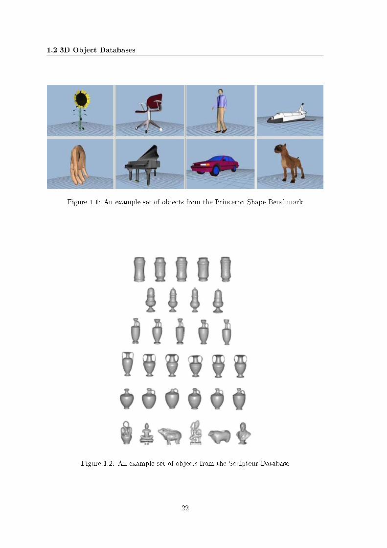
PSB is a publicly available database containing 1814 models, categorized into generalclasses such as animals, humans, plants, household objects, tools, vehicles, buildings, etc.[23] (see Figure 1.1). An important feature of the database is the availability of two equallysized sets. One of them is a training set (90 classes) reserved for tuning the parametersinvolved in the computation of a particular shape descriptor, and the other for testingpurposes (92 classes), with the parameters adjusted using the training set.
SCU is a private database containing over 800 models corresponding to mostly archae-ological objects residing in museums [24, 25]. So far, 513 of the models have been classiedinto 53 categories of comparable set sizes, including utensils of ancient times such as am-phorae, vases, bottles, etc.; pavements; and artistic objects such as human statues (partand whole), gurines, and moulds. An example set of SCU objects is shown in Figure 1.2.The database is augmented by articially generated 3D objects such as spheres, tori, cubes,
20

3D Object Retrieval
cones, etc., collected from the web. The meshes in SCU are highly detailed and reliablein terms of connectivity and orientation of triangles. The following gures illustrate thesignicant distinction between PSB and SCU in terms of mesh resolution. The averagenumber of triangles in SCU and in PSB is 175250 and 7460 respectively leading to a ratioof 23. SCU meshes contain 87670 vertices on the average while for PSB this number is4220. Furthermore, the average triangular area relative to the total mesh area is 33 timessmaller in SCU than in PSB.
SHREC-W has been released for the Watertight track of the Shape Retrieval Contest(SHREC) in 2007 [28, 26]. It consists of 400 watertight meshes of high resolution, classiedinto 20 equally sized classes such as human, cup, glasses, octopus, ant, four-legged animal,etc. Classication semantics in SHREC-W are largely induced by topological equivalencesas shown in Figure 1.3. Accordingly, SHREC-W constitutes a challenging test environmentfor geometry-based shape description methods.
ESB is another database that has been used in the SHREC'07 event and consists of 865closed triangulated meshes, which represent engineering parts (Figure 1.4) [28, 29]. Thisdataset is classied into a ground truth classication with two levels of hierarchy. Overallthere are three super-classes, namely, at-thin object, rectangular-cubic prism, and solid ofrevolution, which are further categorized into 45 classes. It is particularly interesting to seethe performance of 3D shape descriptors on such a database, as CAD oers an importantapplication domain for content-based 3D shape retrieval.
The existence of widely accepted ground truth is a crucial aspect for objective andreproducible eectiveness evaluation [2]. Accordingly, obtaining ground truth data consti-tutes a fundamental problem, which should be addressed by researchers working in the eldof content-based retrieval. The most rigorous attempt to determine 3D object semanticshas been made by the Princeton group [23] and PSB has been a standard test environmentsince 2004. The approach to generate ground truth data for PSB has been to associate,to each semantically homogeneous group of objects, a class name representing an atomicconcept (e.g., a noun in the dictionary) (see [23] for details). The process has been car-ried out by computer science students that were not expected to be experts in semantics.Sculpteur, on the other hand, is a more specialized database containing cultural heritageobjects that ideally require expert intervention for ground truth classication. Manufac-turing styles, periods, places and artists constitute basic entities of an ontology that wouldexplicitly specify the domain of cultural heritage information. However, is it possible toderive such entities from the shape information contained in an object alone? The answeris not clear for the time being. Furthermore, the priorities of eld experts, such as archae-ologists, art historians, museum scientists, can be somewhat orthogonal to what is aimedat in machine learning. For instance, to an archaeologist, even a scratch on the surfaceof an ancient amphora may contain valuable information to determine its manufacturingperiod. On the other hand, a retrieval or classication algorithm would most probablyconsider this scratch as noise or small shape variation that should be discarded in the rstplace. Nevertheless, these conceptual diculties have not prevented us from creating ourown ground truth for SCU. Together with Helin Duta§ac1, we have created a hierarchicalclassication for SCU objects. In determining the categories, we have been driven by formand functionality. The rst two levels of hierarchy in our classication are given in thesequel.
1Helin Duta§ac is with the Bo§aziçi University Signal and Image Processing Laboratory:http://busim.ee.boun.edu.tr/∼helin/.
21
1.2 3D Object Databases
Figure 1.1: An example set of objects from the Princeton Shape Benchmark
Figure 1.2: An example set of objects from the Sculpteur Database
22

3D Object Retrieval
Figure 1.3: The SHREC-W Database and the associated classication
Figure 1.4: An example set of objects from the Purdue Engineering Shape Benchmark
23

1.3 Background on 3D Shape Descriptors
• Utensil
Jar/Jag/Vase
Sugar caster
Amphora
Pilgrim bottle
Bowl
Carafe
Lamp
• Computer-Generated Articial Object
Humanoid
Chess piece
Sphere
Torus
Eight
Cone
Cube
• Pavement
• Artistic Object
Statue
Mould
Relievo
Diverse
1.3 Background on 3D Shape Descriptors
Although the research on 3D shape descriptors for retrieval and classication has startedjust a decade ago or so, there is a considerable amount of work reported so far. Themost up-to-date and complete reviews in this rapidly evolving eld are given in [2, 5, 3].In addition, the reference [23] is useful for a quick scan of practical schemes. Due tothe variety and abundance of the methods, there is no universally accepted taxonomyof 3D shape descriptors. In our review, we preferred to provide a general classication,emphasizing the specic way to exploit the geometrical or topological shape informationcontained in the 3D object. More detailed accounts can be found in [2, 3, 5]. Accordingto our generality criterion, we ended up with the categories shown in Table 1.1.
In the following, we describe the rst three categories of our taxonomy, i.e., histogram-based, transform-based, and graph-based descriptors. Regarding 2D Image-based methods,the work in [54] provides a comprehensive overview. For the remainder, we invite thereader to consult the references given in Table 1.1, or for a quicker scan, the surveys in[2, 3, 5, 54].
24

3D Object Retrieval
Table 1.1: A Taxonomy of 3D Shape DescriptorsCategory Examples
Histogram-Based Cord and Angle Histograms [18, 30, 31]Shape Distributions [32]Generalized Shape Distributions [33]Shape Histograms [34]Extended Gaussian Images [35, 36]3D Hough Transform [37, 38]Shape Spectrum [37]
Transform-Based Voxel-3D Fourier Transform (3DFT) [39]Distance Transform-3DFT and Radial Cosine Transform [40]Angular Radial Transform [41]PCA-Spherical Harmonics [42, 43, 44]Rotation Invariant Spherical Harmonics [45, 16]Spherical Wavelet Transform [46]
Graph-Based Multiresolution Reeb Graphs [47, 48]Skeletal Graphs [49]
2D Image-Based Silhouette Descriptor [17]Depth Buer Descriptor [17]Lighteld Descriptor [50]
Other Methods Spin Images [51]3D Zernike Moments [52]Reective Symmetry Descriptor [53, 19]
1.3.1 Histogram-Based Methods
A vast majority of 3D shape descriptors can be classied under the heading of histogram-based methods. The term histogram is referred to as an accumulator that collects numericalvalues of certain attributes of the 3D object. In this respect, not all the methods presentedin the sequel are true histograms in the rigorous statistical sense of the term, but they allshare the philosophy of accumulating a geometric feature in bins dened over the featuredomain.
In [18, 30], Paquet et al. have presented cord and angle histograms (CAH ) for matching3D objects. A cord, which is actually a ray segment, joins the barycenter of the mesh with atriangle center. The histograms of the length and the angles of these rays (with respect to areference frame) are used as 3D shape descriptors. One shortcoming of all such approachesthat simplify triangles to their centers is that they do not take into consideration thevariability of the size and shape of the mesh triangles. First, because triangles of allsizes have equal weight in the nal distribution; second, because the triangle orientationscan be arbitrary, so that the centers may not represent adequately the impact of thetriangle on the shape distribution. In [31], following similar ideas as in [18, 30], Paquetand Rioux have considered the angles between surface normals and the coordinate axes. Inthese approaches [18, 30, 31], the histograms are constructed always in univariate manneralthough it is also possible to consider multivariate histograms. Paquet and Rioux haveargued that the bivariate histogram of the angles between the surface normal direction andthe rst two axes of the reference frame is sensitive to the level of detail at which the object
25

1.3 Background on 3D Shape Descriptors
is represented. They have supported their claim by the example of two pyramids: one withthe sides formed by inclined planes and the other with the sides formed by a stairway-like makeup. However, our experience shows that considering multivariate informationproves to be more eective than merely concatenating univariate histograms for a retrievalapplication, as explained and supported by experiments in Sections 4.6.2 and 4.8.1.
In the shape distributions approach [32], Osada et al. have used a collection of shapefunctions, i.e., geometrical quantities computed by randomly sampling the 3D surface.Their shape functions list as the distance of a surface point to the origin, the distancebetween two surface points (D2 ), the area of the triangle dened by three surface points,the volume of the tetrahedron dened by four surface points and the angle formed by threerandom surface points. The descriptors become then the histograms of a set of these shapefunctions. The randomization of the surface sampling process improves the estimation overPaquet et al.'s [18] approach, since in this way, one can obtain a more representative anddense set of the surface points. The histogram accuracy can be controlled by changing thesample size. This quite appealing method suers from the fact that the shape functionsmentioned above are not specic enough to describe the 3D shape eectively. The poorretrieval performance of these approaches has been usually attributed to their global nature.The more recent generalized shape distributions (GSD) [33] partly overcome this dicultyby a 3D" histogram where two dimensions account for local and global shape signaturesand one for distances between local shape pairs. However, the improvement provided byGSD is not sucient to raise this methodology to the discrimination level of its competitors.
Ankerst et al. have used shape histograms for the purpose of molecular surface analysis[34]. A shape histogram is dened by partitioning the 3D space into concentric shellsand sectors around the center of mass of a 3D model. The histogram is constructed byaccumulating the surface points in the bins (in the form of shells, sectors, or both) basedon a nearest-neighbor rule. Ankerst et al. illustrate the shortcomings of Euclidean distanceto compare two shape histograms and make use of a Mahalanobis-like quadratic distancemeasure taking into account the distances between histogram bins. Since the approachproceeds with voxel data, 3D objects represented by polygonal meshes need to be voxelizedprior to descriptor extraction.
Extended Gaussian image (EGI ), introduced by Horn [35], and its variants [36, 55, 56]can be viewed as another class of histogram-based 3D shape descriptors. An EGI consistsof a spherical histogram with bins indexed by (θj , φk), where each bin corresponds to somequantum of the spherical azimuth and elevation angles (θ, φ) in the range 0 ≤ θ < 2πand 0 ≤ φ < π. The histogram bins accumulate the count of the spherical angles of thesurface normal per triangle, usually weighted by triangle area. An important extension hasbeen proposed by Kang and Ikeuchi who considered the normal distances of the trianglesto the origin [36]. Accordingly, each histogram bin accumulates a complex number whosemagnitude and phase are the area of the triangle and its signed distance to the originrespectively. The resulting 3D shape descriptor is called complex extended Gaussian image[36].
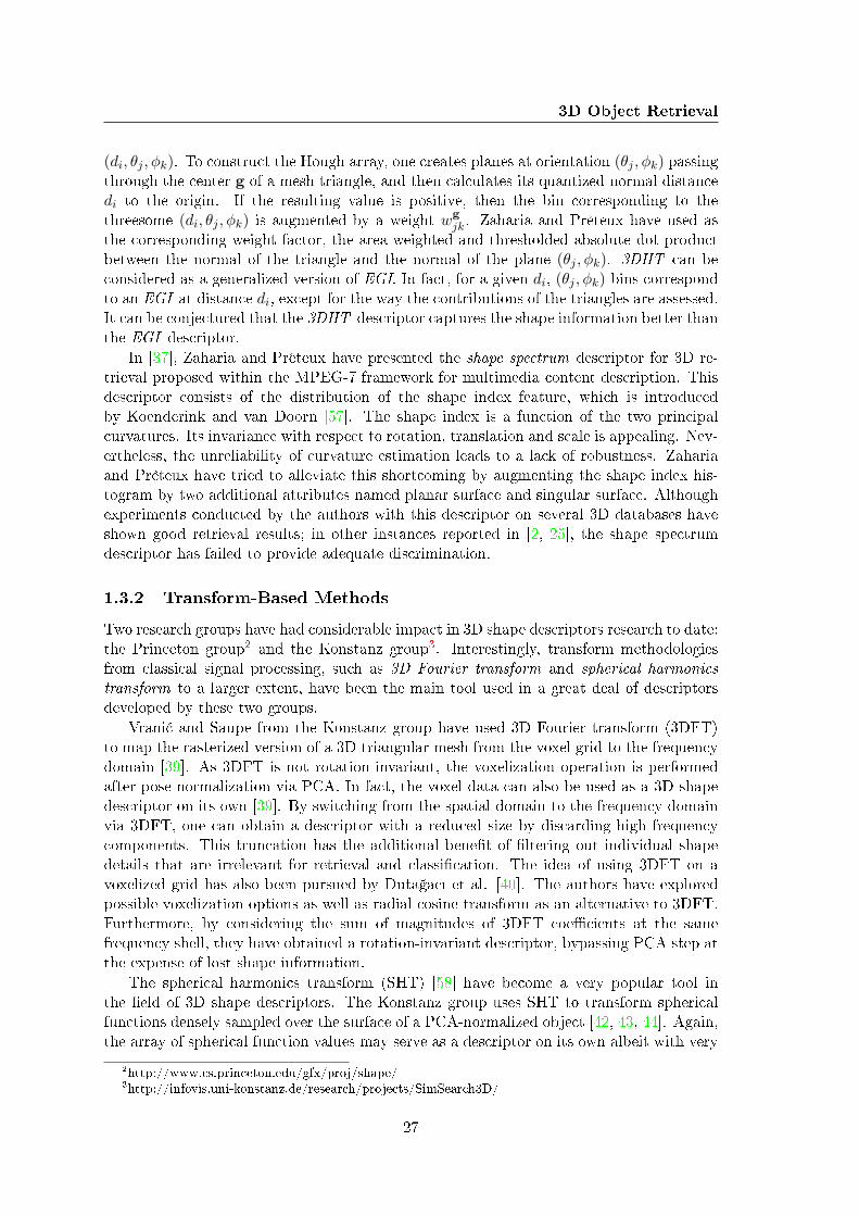
In [37, 38], Zaharia and Prêteux have introduced the 3D Hough transform descriptor(3DHT ) as a histogram constructed by the accumulation of points over planes in 3D space.A plane is uniquely dened by the triple (d, θ, φ), where d is its normal distance to theorigin, and the pair (θ, φ) is the azimuth and elevation angles of its normal, respectively.A nite family of planes can be obtained by the uniform discretization of the parameters(d, θ, φ) over the domain 0 ≤ d ≤ dmax,0 ≤ θ < 2π, and 0 ≤ φ < π. This familyof planes corresponds to a series of spherical histograms where each bin is indexed by
26
3D Object Retrieval
(di, θj , φk). To construct the Hough array, one creates planes at orientation (θj , φk) passingthrough the center g of a mesh triangle, and then calculates its quantized normal distancedi to the origin. If the resulting value is positive, then the bin corresponding to thethreesome (di, θj , φk) is augmented by a weight wg
jk. Zaharia and Prêteux have used asthe corresponding weight factor, the area-weighted and thresholded absolute dot productbetween the normal of the triangle and the normal of the plane (θj , φk). 3DHT can beconsidered as a generalized version of EGI. In fact, for a given di, (θj , φk)-bins correspondto an EGI at distance di, except for the way the contributions of the triangles are assessed.It can be conjectured that the 3DHT -descriptor captures the shape information better thanthe EGI -descriptor.
In [37], Zaharia and Prêteux have presented the shape spectrum descriptor for 3D re-trieval proposed within the MPEG-7 framework for multimedia content description. Thisdescriptor consists of the distribution of the shape index feature, which is introducedby Koenderink and van Doorn [57]. The shape index is a function of the two principalcurvatures. Its invariance with respect to rotation, translation and scale is appealing. Nev-ertheless, the unreliability of curvature estimation leads to a lack of robustness. Zahariaand Prêteux have tried to alleviate this shortcoming by augmenting the shape index his-togram by two additional attributes named planar surface and singular surface. Althoughexperiments conducted by the authors with this descriptor on several 3D databases haveshown good retrieval results; in other instances reported in [2, 25], the shape spectrumdescriptor has failed to provide adequate discrimination.
1.3.2 Transform-Based Methods
Two research groups have had considerable impact in 3D shape descriptors research to date:the Princeton group2 and the Konstanz group3. Interestingly, transform methodologiesfrom classical signal processing, such as 3D Fourier transform and spherical harmonicstransform to a larger extent, have been the main tool used in a great deal of descriptorsdeveloped by these two groups.
Vrani¢ and Saupe from the Konstanz group have used 3D Fourier transform (3DFT)to map the rasterized version of a 3D triangular mesh from the voxel grid to the frequencydomain [39]. As 3DFT is not rotation-invariant, the voxelization operation is performedafter pose normalization via PCA. In fact, the voxel data can also be used as a 3D shapedescriptor on its own [39]. By switching from the spatial domain to the frequency domainvia 3DFT, one can obtain a descriptor with a reduced size by discarding high frequencycomponents. This truncation has the additional benet of ltering out individual shapedetails that are irrelevant for retrieval and classication. The idea of using 3DFT on avoxelized grid has also been pursued by Duta§ac et al. [40]. The authors have exploredpossible voxelization options as well as radial cosine transform as an alternative to 3DFT.Furthermore, by considering the sum of magnitudes of 3DFT coecients at the samefrequency shell, they have obtained a rotation-invariant descriptor, bypassing PCA step atthe expense of lost shape information.
The spherical harmonics transform (SHT) [58] have become a very popular tool inthe eld of 3D shape descriptors. The Konstanz group uses SHT to transform sphericalfunctions densely sampled over the surface of a PCA-normalized object [42, 43, 44]. Again,the array of spherical function values may serve as a descriptor on its own albeit with very
2http://www.cs.princeton.edu/gfx/proj/shape/3http://infovis.uni-konstanz.de/research/projects/SimSearch3D/
27
1.3 Background on 3D Shape Descriptors
high dimensionality. SHT is suitable to reduce the descriptor size considerably, yet withoutlosing too much shape information. The so called ray-based or extent (EXT ) descriptorgives the SH-transformed version of the maximal distance from the center of mass asa function of the spherical angle [42]. In [43], Vrani¢ has improved this descriptor byconsidering a collection of extent functions evaluated at concentric spheres with dierentradii, again with SHT-mapping. This latter descriptor, called as radialized extent descriptor(REXT ), proves to be highly discriminating on dierent databases [23, 2].
Funkhouser et al. [45] from the Princeton group have developed a rotation-invariantdescriptor using SHT. The method requires the 3D object to be voxelized in a binaryfashion. 3D voxel data can be interpreted as a collection of spherical functions fr(θ, φ),where r corresponds to the distance from the origin of the voxel grid and (θ, φ) to sphericalcoordinates. The binary function is sampled for a sucient number of radii r = 1, . . . , Rand angles (θ, φ). Each function at a specic radius is SH-transformed and the energiescontained in low frequency-bands are stored in the nal descriptor. In [16], Kazhdan et al.have provided mathematical support for rotation invariance of the descriptor. Basically,this mathematical justication relies on the fact that the energy in a certain frequency bandof the ST does not change when the object is rotated around its center of mass. In the samework [16], they have also demonstrated that many existing descriptors can be renderedrotation-invariant by this approach. The rotation invariance of this class of descriptorsshould be understood with caution as it comes with a certain loss of shape information[16, 59]. In fact, the use of SHT for 3D shape description has been a matter of debatebetween the Princeton and Konstanz groups. The latter argues that PCA normalizationshould be applied prior to SHT and the magnitude of transform coecients should be usedas the descriptor, while the former claims that PCA is unstable and rotation invarianceshould be secured by considering the energies in dierent bands of the transform domain.Both groups support their claims with retrieval experiments in large databases and favortheir individual standpoints. This discrepancy might be due to database dierences and/orspecic implementation details.
1.3.3 Graph-Based Methods
Graph-based approaches are fundamentally dierent from other vector-based descriptors.They are more elaborate and complex, in general harder to obtain; but they have thepotential of encoding geometrical and topological shape properties in a more faithful andintuitive manner than vector-based descriptors. However, they do not generalize easily toall representation formats and they require dedicated dissimilarity measures and matchingschemes. Due to their complexity in extraction and matching stages, they are not veryecient for general-purpose retrieval applications. We note that, using tools from spectralgraph theory, some part of the information contained in a graph can be encoded in the formof numerical descriptions. Nevertheless, the lack of a vector representation by constructionprevents the use of a great deal of learning algorithms for classication. Although theemphasis in the present work is on vector-based descriptors, we include two representativestudies for the completeness of the account: multiresolution Reeb graphs [47, 48] and skeletalgraphs [49]. The works in [60, 61, 62] and references therein include a comprehensive listof other graph-based representations and matching methods.
Hilaga et al. [47] have introduced the concept of topology matching for 3D objectretrieval. The algorithm relies on constructing Reeb graphs at multiple levels of resolution ofa function µ dened over the object's surface. The function µ can be the height of a point on
28

3D Object Retrieval
the surface, the curvature value or the integrated geodesic distance at that point. Accordingto the function chosen, the resulting descriptor enjoys certain invariance properties. Eachnode in each such graph corresponds to a connected component of the object in the sensethat µ-values in that component fall within the same interval determined by the resolutionat which the graph is constructed. Parent-child relationships between nodes representadjacent intervals of these µ-values for the contained object parts. Furthermore, a graphat a coarser level is encoded as the ancestor of a graph at a ner level. Obviously, atthe coarsest level, the graph consists of a single node accounting for the whole object.The theoretical support of this multiresolution approach is that, for a given object, as theresolution gets ner, the nodes of the resulting graph corresponds to the singular pointsof the µ-function. It has been demonstrated that such critical point locations are valuablein studying the topology of the underlying object [63]. Sophisticated heuristics have beenproposed to match two graphs for similarity assessment in [47] and in [25, 48]. Moreover,in the latter two works, the graph has been augmented with other vector-based descriptorsto improve the discrimination ability.
In [49], the authors have described a method for searching and comparing 3D objectsvia skeletal graph matching. The objective is to build an interactive system that allowspart matching. The visualization of the results is facilitated by skeletal graphs, whichalso help the user to rene and interactively change his/her query. The skeletal graph isobtained from object voxel data as a directed acyclic graph (DAG). Each node of the DAGis associated with a set of geometric features and a signature vector that encodes topologicalinformation. The latter is called a topological signature vector (TSV), which is derivedfrom the eigendecomposition of the graph's adjacency matrix. The matching procedureconsists of two stages where rst a topology matching between the query database graphs isperformed on a per node basis. The second (optional) stage consists of geometry matching.It can be used to rene the possible set of retrieved database objects. However, the authorshave not elaborated on this issue further.
1.4 Similarity Measures
The assessment of similarity between two objects is usually performed by computing adissimilarity measure between their corresponding descriptors. Accordingly, throughoutthe thesis, we will use the terms similarity and dissimilarity (or distance) interchangeably.The context will clarify the distinction. A similarity function sim : F × F → R can beviewed as the abstract inverse to a dissimilarity function dist : F × F → R, where F isthe space of generic descriptors f . Ideally, we expect that dist(f, f ′) decreases (sim(f, f ′)increases), as the level of semantic similarity between the corresponding objects gets higher.The dissimilarity measure dist may enjoy the following properties [3]:
(1) Identity : ∀f ∈ F , dist(f, f ′) = 0.
(2) Positivity : ∀f 6= f ′ ∈ F , dist(f, f ′) > 0.
(3) Symmetry : ∀f, f ′ ∈ F , dist(f, f ′) = dist(f ′, f).
(4) Triangle inequality : ∀f, f ′, f ′′ ∈ F , dist(f, f ′′) ≤ dist(f, f ′) + dist(f ′, f ′′).
A dissimilarity measure satisfying all of the four properties listed above is said to be ametric. A pseudo-metric satises all metric properties but positivity, and a semi-metricsatises only the rst three properties. A function satisfying the triangle inequality is often
29

1.5 Evaluation Tools for Retrieval
desirable, since it can make retrieval more ecient [64]. These properties are abstract in thesense that the dissimilarity function can be dened on arbitrary descriptor spaces (e.g.,for graphs, or even directly for 3D objects). In the present work, we restrict ourselvesto the case of vector-based descriptors, that is, when the descriptor space F is a nitevector space. Classical dissimilarity measures for vector-based descriptors are Lp-distances(p > 0), Bhattacharyya distance, χ2-divergence [65], symmetricized versions of Kullback-Leibler divergence [65], earth mover's distance [66] and histogram intersection distance [67](see Appendix B for denitions).
Regarding similarity measures, we would like to underline two points:
• A distance function dist on a nite-dimensional vector space F usually arises as adiscretized version of a continuous functional dist on an innite space of continuousfunctions F . Suppose that f is a function describing a certain object by mappingmultidimensional attributes t ∈ Rm to reals. A functional dist, quantifying theamount of variation between f and another descriptor function f ′ can be genericallywritten as
dist(f, f ′) =∫
t∈Rm
η(f(t), f ′(t)
)dt,
where η is a point-wise dissimilarity function, e.g., for L1, η(·, ·) = | ·−· |. In practice,an object is described by a nite vector of f(t)-values, i.e., f = [f(t1), . . . , f(tN )], inwhich case the above integral should be discretized as
dist(f , f ′) =∑
n
η(f(tn), f ′(tn)
)∆tn, (1.1)
where ∆tn is the discretization step size. If the space of multidimensional attributesis uniformly partitioned, ∆tn becomes constant, hence aects the value of the inte-gral by a constant amount for all descriptors, and consequently, it can be dropped.Otherwise, it must be taken into account in distance calculation.
• The dissimilarity between two objects can be made invariant against certain typesof transformations Γ by the following formula:
distΓ-invariant(f , f ′) = minΓ∈GΓ
dist(f ,Γ(f ′)),
where GΓ is the group of transformations that the objects might have been undergoneprior to descriptor extraction. Since we want that the distance function captures onlyintrinsic shape dierences and commonalities, GΓ should consist of extrinsic eectssuch as translation, rotation, isotropic rescaling or a combination of these. Theabove formula is practical only when the transformation can be directly eected onthe descriptor, without recomputing it for every possible transformed version of theobject. In Section 2.4, we concretize this idea of securing invariance at matching stageand develop such a measure, easily applicable for density-based shape descriptors.
1.5 Evaluation Tools for Retrieval
In this section, we summarize the most commonly used statistics for measuring the per-formance of a shape descriptor in a content-based retrieval application [23].
30

3D Object Retrieval
• Precision-Recall curve. For a query q that is a member of a certain class C of size|C|, Precision (vertical axis) is the ratio of the relevant matches Kq (matches thatare within the same class as the query) to the number of retrieved models Kret, andRecall (horizontal axis) is the ratio of relevant matches Kq to the size of the queryclass |C|:
Precision =Kq
Kret,
Recall =Kq
|C|.
Ideally, this curve should be a horizontal line at unit precision.
• Nearest Neighbor (NN). The percentage of the rst-closest matches that belongto the query class. A high NN score indicates the potential of the algorithm in aclassication application.
• First-tier (FT) and Second-tier (ST). First-tier is the recall when the numberof retrieved models is the same as the size of the query class and second-tier is therecall when the number of retrieved models is two times the size of the query class.
• E-measure. This is a composite measure of the precision and recall for a xednumber of retrieved models, e.g., 32, based on the intuition that a user of a searchengine is more interested in the rst page of query results than in later pages. E-measure is given by
E =2
1Precision + 1
Recall
.
• Discounted Cumulative Gain (DCG). A statistic that weights correct resultsnear the front of the list more than those appearing later, under the assumptionthat the user is interested more with the very rst items displayed. To calculate thismeasure, the ranked list of retrieved objects is converted to a list L, where an elementLk has value 1 if the kth object is in the same class as the query and otherwise hasvalue 0. Discounted cumulative gain at the kth rank is then dened as
DCGk =
Lk, k = 1,
DCGk−1 + Lklog2(k) , otherwise.
The nal DCG score for a query q ∈ C is the ratio of DCGKmax to the maximumpossible DCG that would be achieved if the rst |C| retrieved elements were in theclass C, where Kmax is the total number of objects in the database. Thus DCG readsas
DCG =DCGKmax
1 +∑Cq
k=21
log2(k)
.
• Normalized DCG (NDCG). This is a very useful statistic based on averagingDCG values of a set of algorithms on a particular database. NDCG gives the rel-ative performance of an algorithm with respect to the others tested under similarcircumstances. A negative value means that the performance is below the average;similarly a positive value indicates an above-the-average performance. Let DCG(A)
31

1.5 Evaluation Tools for Retrieval
be the DCG of a certain algorithm A and DCG(avg) be the average DCG values of aseries of algorithms on the same database, then NDCG for the algorithm A is denedas
NDCG(A) =DCG(A)
DCG(avg)− 1.
All these quantities are normalized within the range [0, 1] (except NDCG) and higher valuesreect better performance. In order to give the overall performance of a shape descriptoron a database, the values of a statistic for each query are averaged over all available queriesto yield a single average performance gure. The retrieval statistics presented in this workare obtained using the utility software included in PSB [23].
32

Chapter 2
Density-Based
3D Shape Description
Density-based shape description is a generative model, aiming to encode geometrical shapeproperties contained within a class of 3D objects. This generative model relies on theidea that, associated with each shape concept, there is an underlying random process,which induces a probability law on some local surface feature of choice. We assume thatthis probability law admits a probability density function (pdf), which, in turn, encodesintrinsic shape properties to the extent achieved by the chosen feature. Shared or individualaspects of two shape concepts can be quantied by measuring the variation between theirassociated feature pdfs. The surface feature can be general, such as the distance froma predened origin, or specic, for instance, involving local dierential structure on thesurface. As one moves from general to specic, discrimination power of a local feature andits pdf increase. General features can be joined together in order to obtain more specicmultivariate features. With its ability to process multivariate local feature information, thedensity-based framework generates a family of 3D shape descriptors on which we elaboratein this chapter.
A density-based descriptor of a 3D shape is dened as the sampled pdf of some surfacefeature, such as radial distance or direction. The feature is local to the surface patch andtreated as a random variable. At each surface point, one has a realization (observation) ofthis random variable. For instance, if the surface is given in terms of a triangular mesh asit is generally assumed in this work, the set of observations can be obtained from verticesand/or triangles. To set the notation, let S be a random variable dened on the surface ofa generic 3D object O and taking values within a subspace RS of Rm. Let fS|O , fS(·|O)be the pdf of S for the object O. This pdf can be estimated using the set of observationssk ∈ RSK
k=1 computed on the object's surface. In the sequel, random variables appear asuppercase letters while their specic instances as lowercase. Suppose furthermore that wehave specied a nite set of points within RS , denoted as RS = tn ∈ RSN
n=1, called thetarget set. The density-based descriptor fS|O for the object O (with respect to the featureS) is then simply an N -dimensional vector whose entries consist of the pdf samples at thetarget set, that is, fS|O = [fS(t1|O), . . . , fS(tN |O)].
Density-based shape description consists of three main stages:
(1) First, in the design stage, we choose good local features that accumulate to globalshape descriptors. Good features are computationally feasible and discriminative(Sections 2.1.1 and 2.1.2).
33

2.1 Local Characterization of a 3D Surface
Figure 2.1: Density-based shape description
(2) Second, in the target selection stage, we focus on determining the pdf evaluationpoints sampled in RS , i.e., determining the target set RS (Section 2.1.3).
(3) Finally, we address the computational stage, in search of an ecient computationalscheme to estimate fS(t|O) at designated targets t ∈ RS . In the present work, weuse the kernel density estimation (KDE) approach coupled with a fast algorithm, thefast Gauss Transform (FGT) [9] (Section 2.2).
The nal output of these stages is the shape descriptor vector fS|O, whose componentsfS(tn|O) are the pdf values evaluated at the target set RS . Figure 2.1 illustrates thisdescriptor extraction process.
The fact that the description scheme is based on pdfs allows one to use this specialstructure for several ends. For instance, in Section 2.3, we present two descriptor manip-ulation tools: marginalization and probability density pruning. Marginalization integratesout the information contained in a subset of feature components from a multivariate pdf.This can help us to explore eventual redundancies of certain components in a multivariatelocal feature. Probability density pruning, on the other hand, eliminates negligible pdfvalues from the descriptor by thresholding the prior feature density fS , which is calculatedby averaging conditional pdfs fS|Ou
over a representative set of objects O = Ou. Bothof these tools can be employed to reduce descriptor dimensionality without loss of per-formance. Another advantage that the pdf structure oers is to secure invariance againstcertain types of object transformations at the matching stage, without the need of recom-puting the descriptor for every possible transformation. In Section 2.4, we develop sucha similarity measure and show its invariance under specic conditions. In Section 2.5, wenalize the chapter by providing an implementation summary of the density-based shapedescription algorithm.
2.1 Local Characterization of a 3D Surface
2.1.1 Local Surface Features
In this section, we describe the local geometric features that we use to characterize 3Dsurfaces (see Figure 2.2). Our approach is inductive in the sense that we start by simple
34

Density-Based 3D Shape Description
Figure 2.2: Illustration of local surface features
features with minimal requirements about the underlying surface and continue with moresophisticated ones in order to arrive to an extensive pointwise characterization.
Zero-Order Features
The most basic type of local information about a point lying on a 3D surface are its coordi-nates. Zero-order features require solely that the underlying surface be continuous withoutany further higher-order dierential structure: a condition, which is usually fullled for 3Dmeshes.
• Radial distance R measures the distance of a surface point Q to the origin (centroid)and has taken place in many dierent shape descriptors [32, 30]. Although it is notan eective shape feature all by itself, when used jointly with other local surfacefeatures, it helps us to decouple the feature distribution at varying distances fromthe object's center of mass.
• Radial direction R is a unit length vector (Rx, Ry, Rz) collinear with the ray tracedfrom the origin to the surface point Q. This unit-norm vector is obviously scale-invariant. When we augment the R-vector with the radial distance R, the resulting 4-tuple (R, Rx, Ry, Rz) can serve as an alternative to the standard Cartesian coordinaterepresentation of the surface point. However in this parameterization, distance anddirection information are decoupled. We say that the feature R radializes the densityof the feature R. Note also that the range of these features can be determinedindependently. In fact, the vector R lies on the unit 2-sphere, and the scalar R lieson the interval ]0, rmax], where rmax depends on the size of the surface.
35

2.1 Local Characterization of a 3D Surface
First-Order Features
First-order features require rst-order dierentiability, hence the existence of a tangentplane at each surface point. For 3D meshes, each interior point on a mesh triangle hasobviously a tangent plane, which is basically the plane supporting the mesh triangle towhich the point belongs. At vertices, even though the situation is more complex, one cancompute a tangent plane by using the 1-ring of the vertex point [68].
• Normal direction N is simply the unit normal vector at a surface point and repre-sented as a 3-tuple (Nx, Ny, Nz). Similar to the radial direction R, the normal N isscale-invariant.
• Radial-normal alignment A is the absolute cosine of the angle between the radial andnormal directions and is computed as A = |〈R, N〉| ∈ [0, 1]. This feature measurescrudely how the surface deviates locally from sphericity. For example, if the localsurface approximates a spherical cap, then the radial and normal directions align,and the alignment A approaches unity.
• Tangent plane distance D stands for the absolute value of the distance between thetangent plane at a surface point and the origin. This scalar feature D is related to theradial distance R by D = RA. The joining of D with the normal direction N providesa four-component vector (D, Nx, Ny, Nz) that corresponds to the representation ofthe local tangent plane. As in the radial case, this representation also separates thedistance and direction information associated with the tangent plane.
• In addition to the radial-normal alignment A, the interaction between the surfacenormal vector and the radial direction can be quantied by taking the cross productbetween R and N. The torque feature C = R × N can be considered as a localrotational force when R is viewed as the position of a particle, which is under theinuence of an external force N.
Second-Order Features
The second fundamental form IIQ contains useful dierential geometrical informationabout a surface point Q. This form is dened as IIQ(u) = 〈dNQ(u),u〉, where u is a3-vector lying on the tangent plane and dNQ is the dierential of the normal eld at thepoint Q [69]. The dierential dNQ is a linear map, measuring how the normals pull awaywithin a neighborhood of Q, along a direction pointed by an arbitrary vector u on thetangent plane. Minimum and maximum eigenvalues of dNQ, called principal curvaturesκ1 and κ2, are also the minimum and maximum of the second fundamental form IIQ.They measure the minimum and maximum rates of change at which the normal deviatesfrom its original direction at Q. Given the principal curvatures, one can obtain a uniquelocal characterization up to a scale [69]. By denition, IIQ requires second-order dieren-tiability. This condition is never fullled for a 3D mesh, which is just piece-wise planar(hence at most rst-order dierentiable). Nevertheless, IIQ can be computed by tting atwice-dierentiable surface patch to the vertex point and invoking standard formulae fromdierential geometry [69], or by discrete approximation using the mesh triangles withinthe 1-ring of the vertex point [68, 70].
• Shape index SI, rst proposed by Koenderink and van Doorn [57], provides a localcategorization of the shape into primitive forms such as spherical cap and cup, dome,
36

Density-Based 3D Shape Description
rut, ridge, trough, or saddle (see Figure 2.3). In the present work, we consider theparameterization proposed in [71] given by
SI =12−(
2π
)arctan
(κ1 + κ2
κ1 − κ2
).
SI is conned within the range [0, 1] and not dened when κ1 = κ1 = 0 (planarpatch). Since the shape index SI is a function of the principal curvatures, it isconsidered as a second-order feature. It not only inherits the translation and rotationinvariance of the principal curvatures, but also is a unitless quantity hence scale-invariant.
Figure 2.3: Shape index characterizes the local surface into a set of representatives.
Construction of a Multivariate Feature
Each of the above features reects a certain incomplete aspect of the local shape. Wecan obtain a more thorough characterization of the surface point Q by constructing themultivariate feature (R, R, N, SI) as explained below:
(1) The radial distance R restricts the point to the surface of a sphere around the object'scenter of mass.
(2) The radial direction R spots the location of the point on the sphere.
(3) The normal direction N associates a rst-order dierential structure, i.e., a tangentplane with the point.
(4) The shape index SI adds the more rened categorical surface information in termsof shape primitives.
The construction process is illustrated in Figure 2.4. In the density-based shape descriptionframework, the pdf of these features, taken together in the form of a higher dimensionaljoint feature, would become a global descriptor, summarizing every single piece of localshape information up to second-order. However, this multivariate feature constructionfollowed by pdf estimation is not without a caveat. Observe that the (R, R, N, SI) is an 8-component feature with an intrinsic dimensionality of 6 as it takes values within ]0, rmax]×S2×S2× [0, 1], where S2 denotes the unit 2-sphere. This fairly high dimensionality brings
37

2.1 Local Characterization of a 3D Surface
Figure 2.4: Construction of a multivariate feature
in concomitant problems of pdf estimation accuracy, high computation time and hugestorage size as will be claried in the upcoming sections.
Based on the above discussion, the features presented in this section can also be clas-sied into two types: primary and auxiliary. The features involved in the full character-ization up to second order as described above, namely, R, R, N and SI are denominatedas primary. We call the remaining tangent plane distance D, the radial-normal alignmentA and the radial-normal torque C features as auxiliary, in the sense that they encode in-teractions between primary features. From a computational viewpoint, auxiliary featurescan be derived from primary ones. In Table 2.1, we summarize the properties of our localsurface features.
Table 2.1: Classication and Invariance of Local Surface FeaturesClassication Invariance
Feature Order Type Translation Rotation Scale
Radial Distance Zero Primary No Yes NoRadial Direction Zero Primary No No YesNormal Direction First Primary Yes No YesT-plane Distance First Auxiliary No Yes No
Alignment First Auxiliary No Yes YesTorque First Auxiliary No No Yes
Shape Index Second Primary Yes Yes Yes
38

Density-Based 3D Shape Description
From a practical viewpoint, by joining primary and auxiliary features, we can designthe following multivariate pdf-based descriptors with manageable dimension in terms ofpdf estimation accuracy, descriptor computation time and storage size:
• Radial -descriptor is the pdf of the Cartesian coordinate representation (R, R) of thesurface point.
• T-plane-descriptor is the pdf of the (D, N)-feature and aggregates the local tangentplane information.
• Torque-descriptor is the pdf of a radialized version of the torque feature, given by(R,C).
• Sec-Order -descriptor is the pdf of the (R,A, SI)-feature, which radializes the auxil-iary alignment information A together with the second-order feature SI.
In the experiments, we explore the discrimination ability of these designed features andtheir variants.
2.1.2 Feature Calculation
A triangular meshM is given in terms of a union of K trianglesM =⋃K
k=1 Tk, where eachtriangle Tk is associated with a triplet of 3D points (Ak, Bk, Ck), represented by a triplet of3-vectors (ak,bk, ck). Regarding an m-dimensional local feature S = (S1, . . . , Sm), we canobtain the observations by evaluating the value of S at the barycenter of each triangle orat each vertex. However, the mesh resolution might not be very ne and/or the trianglesmight have arbitrary shapes and sizes. Accordingly, the feature value at the barycenter orat the vertex may not be the most representative one. The shape of the triangle shouldbe in some way taken into account in order to reect the local feature characteristics morefaithfully. The expected value of the local feature E S|T over a generic triangle T isthought to be more reliable than the feature value sampled only at a single point, e.g, thebarycenter or the vertex.
Consider T as an arbitrary triangle in 3D space with vertices A, B, and C representedby the vectors a, b, and c respectively (see Figure 2.5). By noting e1 = b−a and e2 = c−a,we can obtain a parametric representation for an arbitrary point Q inside the triangle T asp = a+ xe1 + ye2, where the two parameters x and y satisfy the constraints: x, y ≥ 0 andx + y ≤ 1. Assuming that the point Q is locally uniformly distributed inside the triangleT , the expected value of the ith component of S, denoted by E Si|T, is given by
E Si|T =∫∫
ΩSi(x, y)f(x, y)dxdy, i = 1, . . . ,m. (2.1)
where Si (x, y) is the feature value at (x, y) and f (x, y) is the uniform probability densityfunction of the pair (x, y) over the domain Ω = (x, y) : x, y ≥ 0, x + y ≤ 1. Accordingly,f (x, y) = 2 when (x, y) ∈ Ω or zero otherwise1. The integration is performed over thedomain Ω. To approximate Eq. 2.1, we can apply Simpson's one-third numerical integra-tion formula [72]. Avoiding the arbitrariness in vertex labeling by considering the threepermutations of the labels A, B, and C, we get three approximations, which are in turnaveraged to yield:
1Note that the area of the domain Ω is 1/2, thus f (x, y) = 2 whenever (x, y) ∈ Ω.
39

2.1 Local Characterization of a 3D Surface
Figure 2.5: Parameterization of a point on a 3D triangle
E Si|T≈ (1/27)(Si(a) + Si(b) + Si(c)))+(4/27)(Si((a + b)/2) + Si((a + c)/2) + Si((b + c)/2))+(4/27)(Si((2a + b + c)/4) + Si((a + 2b + c)/4) + Si((a + b + 2c)/2)).
(2.2)
Notice that Eq. 2.2 boils down to taking a weighted average of the feature valuescalculated at nine adequately chosen points on the triangle. For meshes with low resolution,this averaging has the eect of smoothing the observations so that the subsequent pdfestimation can be performed more accurately, thus resulting in more reliable descriptors.In Section 4.2.1, we support this claim by experimentation. As a side remark, we alsopoint out the above averaging scheme can be applied to higher-order moments and cross-correlations of feature components.
It is also worth noting that the Simpson averaging scheme does not apply to the shapeindex SI. The computation of the latter feature involves curvature estimation, whichcan be carried on a per vertex basis as in [70]. In order to obtain realizations of SI pertriangle, we take the average of the values at the three vertex points forming the triangle.In a similar way to Simpson averaging, this adds an implicit smoothing eect to the shapeindex calculation.
2.1.3 Target Selection
We dene the target selection problem as sampling the range of the feature at whichthe pdf is evaluated. Since a density-based descriptor is merely a sampled version ofa continuous pdf, we need to be ecient in choosing density evaluation points. First,we should not include very low density points and second, we should exploit any specialstructure associated with the feature range. The features presented in the previous sectionare either scalar or vector by construction. Sampling the real interval I of a scalar featureis relatively simple. For certain vector features, such as R and N, on the other hand,
40

Density-Based 3D Shape Description
the unit-norm condition implies that the feature lies on the unit 2-sphere S2 and that thecorresponding target points should satisfy this property. In the following, we discuss thesampling of I and S2 separately, providing two dierent methods for each.
Sampling for Scalar Features
The support I = (smin, smax) of a scalar feature S is determined by the lower and upperpercentiles (αmin, αmax) of the distribution of S, dened as
αmin , PrS ≤ smin =∫ smin
−∞fS(s)ds,
αmax , PrS ≥ smax =∫ ∞
smax
fS(s)ds,
where fS(s) is the prior density of the feature S. We set both lower and upper percentilesto a unique value α. The prior density does not contain any object-specic information andis calculated by averaging over a set of representative objects O = Ou : u = 1, . . . , |O|.Concretely, we have
fS(s) =∑
u
fS(s,Ou) =∑
u
fS(s|Ou)PrOu =1|O|
∑u
fS(s|Ou), (2.3)
assuming that all objects are equiprobable, i.e., PrOu = 1/|O|. Once the domain of thepdf is set, the NI targets points remain to be determined. The two methods we considerare given below.
• In uniform sampling, we partition the interval into NI equally spaced (uniform)sub-intervals and take the midpoints as targets.
• In equal probability sampling, we partition the interval into NI equal probabilityregions and take the midpoints as targets. Similar to Max-Lloyd quantization [73],this scheme yields non-uniformly spaced sub-intervals and places more targets toregions of high prior density.
Note that clipping the tails of the distribution is meaningful only if the scalar feature hasa magnitude interpretation (see Figure 2.6), according to which too small and/or too largevalues can be considered as outliers. In fact, for the alignment A and the shape index SI,which both lie on the unit-interval [0, 1], the values near the boundaries are quite indicativeof the local shape. For these, we simply take NI equally spaced points within the unitinterval.
Sampling for Unit-Norm Vector Features
For the radial direction R and the normal direction N , we sample the unit 2-sphere S2 toobtain the targets. We propose again two dierent sampling methods:
• In octahedron subdivision, we consider an octahedron circumscribed by the unitsphere, subdivide into four each of its eight triangles, radially project the new tri-angles on the unit sphere, and iterate a factor of a times the subdivision process.The barycenters of the resulting triangles (after projecting back to the unit sphere)become the target set for direction components. This leads to an approximately
41

2.1 Local Characterization of a 3D Surface
Figure 2.6: Probability density function of R displayed with the lower and upper 1% tailsclipped
uniform partitioning of the sphere as shown in Figure 2.7. The recursion factor a de-termines the number of resulting points NS2 ; e.g., for a = 1, we get NS2 = 8×4 = 32points; for a = 2, we get NS2 = 8× 16 = 128, and in general NS2 = 22a+3.
• In spherical coordinate sampling, we parameterize the unit sphere in terms of sphericalcoordinates (θ, φ). Recall that any point on the sphere can be expressed as a 3-tuplegiven by (cosθsinφ, sinθsinφ, cosφ) where 0 ≤ θ < 2π and 0 ≤ φ < π. Uniformlysampling the θ- and φ-coordinates at Nθ and Nφ points, respectively, results in NS2 =Nθ ×Nφ points. This method, however, does not provide a uniform partitioning ofthe sphere (see Figure 2.7).
Sampling for Arbitrary Vector Features
As pointed out earlier, we can design new features by joining the features presented inSection 2.1.1. In such cases, the target selection range occurs as the Cartesian product ofthe individual ranges of the features involved. (R, R) and (D, N) constitute two cases inpoint: their ranges both consist of the Cartesian product of an interval I on the real linewith the unit 2-sphere S2. This decoupling allows us to sample I and S2 independentlyinto NI and NS2 points respectively, and to take the Cartesian product of the two resultingsets to yield the target set RS of size N = NI ×NS2 . This idea extends naturally to thejoining of L dierent features Sl, l = 1, . . . , L with individual target sets RSl
, l = 1, . . . , L,in which case the nal target set is obtained as the L-fold Cartesian product of RSl
's.
42

Density-Based 3D Shape Description
Figure 2.7: NS2 = 128 points on the unit-sphere obtained by the two methods mentionedin the text: (a) by subdividing an octahedron a = 2 times, (b) by uniformly sampling thespherical coordinates, Nθ = 16 and Nφ = 8
2.2 Kernel Density Estimation
Given a set of independent observations sk ∈ RmKk=1 of a random variable (scalar or
vector) S ∈ Rm, the kernel approach to estimate the probability density value of S at atarget t ∈ Rm is formulated in its most general form as
fS(t) =K∑
k=1
wk |Hk|−1K(H−1
k (t− sk)). (2.4)
where K : Rm → R is a kernel function, Hk is an m × m matrix composed of a set ofdesign parameters called bandwidth parameters (smoothing parameters or scale parame-ters) for the kth observation, and wk is the positive scalar weight associated with the kthobservation. The weights satisfy the constraint
∑k wk = 1 and, if all the observations
are considered as equally likely, we have wk = 1/K,∀k. The contribution of each datapoint sk to the density function fS at a target point t is computed through the kernelfunction K rescaled by the matrix Hk and weighted by wk. Thus KDE involves a data setskK
k=1 with the associated set of weights wkKk=1, the choice of a kernel function K and
the setting of bandwidth parameters HkKk=1.
Historically, the kernel estimate for a univariate pdf f(s), s ∈ R has been rst intro-duced by Rosenblatt [74] as a numerical approximation to the derivative of the distributionfunction F (s) =
∫ s−∞ f(u)du. The method is also known as Parzen window after Parzen
who has generalized the approach and proved consistency and asymptotic normality of theunivariate kernel density estimator [75]. The multivariate generalization is due to Cacoul-los [76]. Scott [77, 78, 7] and Silverman [79, 80, 81] have greatly contributed to the domainby dealing with issues such as the choice of the kernel function and the bandwidth para-meters. Since then, the KDE approach has been a powerful non-parametric data analysismethodology nding several application niches in pattern recognition and computer vision
43

2.2 Kernel Density Estimation
[13, 82, 83].KDE can be viewed as a data smoothing technique overcoming certain limitations of
the classical histogram method [7, 6]. In the histogram, one places a set of equal sized binson the input domain and basically counts the number of observations falling inside eachof them. This approach might become overly restrictive due to two reasons: (i) dependingon the choice of origin, the appearance of the histogram diers signicantly, (ii) all of thesamples falling inside a bin contribute to pdf value equally, no matter how far they arefrom the bin center, leading to non-smooth estimates especially in high dimensions andwhen the number of observations is small. The KDE addresses both of these limitations[6]. First, by construction, there is no need to x an origin in the input domain. Secondand more importantly, the kernel K acts as a convolution lter weighting the observationssk as a function of their distance to the density evaluation point t. In a nutshell, closerobservations contribute more to the pdf estimate and far-away ones less. The smoothingbehavior of the kernel estimator is controlled by the bandwidth parameter(s).
In Section 2.2.1, we put KDE in context and illustrate its discriminativeness for shapedescription. Note that in Appendix C.1, we derive the kernel estimator of a multivariatepdf following [13], paving the way for our discussion in Section 2.2.2 on the crucial issueof bandwidth selection. In Section 2.2.3, we discuss fast computational schemes to makeecient use of KDE for the 3D shape description problem.
2.2.1 KDE in Context
As pointed out in the previous paragraphs, KDE is a general purpose data smoothingtechnique. In the present section, we place this powerful tool in the context of 3D shapedescription and illustrate its discriminativeness using a constructed example. We need rstto instantiate Eq. 2.4 with a particular choice of the kernel function. In the present work,we prefer the Gaussian kernel, in which case Eq. 2.4 becomes
fS(t|O) = (2π)−m/2K∑
k=1
wk|Hk|−1exp(− 1
2(t− sk)T H−2
k (t− sk)). (2.5)
The reason for our choice on the Gaussian kernel is mainly computational. Direct evalu-ation of Eq. 2.5 on a target set tnN
n=1 using a set of observations skKk=1 has O(KN)-
complexity, which might become infeasible or impractical for real-time tasks. The fastGauss transform algorithm [8, 9] alleviates the computational burden by reducing thecomplexity down to O(K + N) (see Section 2.2.3).
To put Eq. 2.5 in context, we make the following points for 3D shape description:
• Observations or sources skKk=1 are the feature values (or vectors) computed on the
surface of an object O. They can be obtained from each of the mesh triangles, vertexpoints or by the averaging scheme described in Section 2.1.2.
• Targets tnNn=1 are the pdf evaluation points so that fS(tn|O)-values constitute the
descriptor vector fS|O = [fS(t1|O), . . . , fS(tN |O)].
• Weights wkKk=1 stand for the strength or the intensity of each of the sources. For
a 3D mesh, a weight wk can be set to the relative area of the mesh triangle (withrespect to the total surface area) over which the feature observation sk is computed.
44

Density-Based 3D Shape Description
• Bandwidth parameters HkKk=1 model the degree of uncertainty about the obser-
vations and control the smoothing bevahiour of the KDE. Appropriate bandwidthselection is a critical issue for all applications using the KDE scheme [84]. Multiplehypotheses can be made prior to the choice of the bandwidth parameters. Eq. 2.5embodies the most general situation in which case the degree of uncertainty abouteach observation varies. It is also possible to impose a unique degree of uncertaintyby assigning a xed bandwidth matrix H to each of the observations in which casewe have Hk = H,∀k.
Discriminativeness of the KDE-based framework
We can analyze the discriminativeness of the KDE-based framework in two closely relatedbut dierent contexts:
• In recognition, we are given a shape O′ and wish to decide whether it is just a perturbedversion of or is completely dierent from a certain shape O. In the former case, agood descriptor should not vary too much from shape O to O′, in an appropriatesense of variation between descriptors. In the latter case, the descriptor must reactmore to dierences. Put in other words, the amount of perturbation is one of thedetermining factors for the shape O′ to be recognized as O or not.
• In the more complicated cases of classication and retrieval, we are faced with theproblem of nding an equivalence relation on a given set of shapes. Depending onthe application, we should assign geometrically, topologically and/or semanticallysimilar shapes into the same equivalence class. All the shapes O′ belonging to acertain equivalence class can be considered as random realizations of an ideal shapeO, which may or may not exist physically but should fulll the idea of the shape classunder question. This platonic view of the aairs subsumes there exists a non-physicalpencil" and all the real physical pencils" are just random realizations of it. In thissetting, the variation among the descriptors of the shapes from the same equivalenceclass should always be uniformly lower than the variation among the descriptors ofthe shapes from dierent equivalence classes.
We will make use of the following simple example to illustrate the discriminativenessof the KDE-based scheme. Let S = sk ∈ RK
k=1 be a set of measurements about a scalarfeature S and S ′ = s′k ∈ R : s′k = sk + εkK
k=1 be a perturbed version of S. We assumethat the set S is non-random and constitutes an ideal set obtained from the surface of ageneric shape O. The set S ′, on the other hand, is non-ideal and random. Randomnessis incorporated through zero-mean independent identically distributed (i.i.d.) randomvariables εk's with variance σ2. This additive perturbation model accounts for randomgeometrical variations of unconstrained amount, e.g., for the radial distance feature R.A small perturbation indicates small shape dierences, while a larger one corresponds tomore fundamental departures from the original shape. Regarding the set S ′, depending onthe type of the context chosen for analysis, we can state the following:
• In recognition, S ′ arises from a noisy" shape O′. The amount of noise, for which σ2
is one possible measure, constitutes a determining factor for the shape O′ to be O ornot.
45
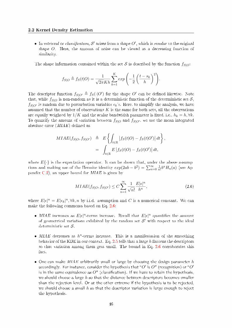
2.2 Kernel Density Estimation
• In retrieval or classication, S ′ arises from a shape O′, which is similar to the originalshape O. Here, the amount of noise can be viewed as a decreasing function ofsimilarity.
The shape information contained within the set S is described by the function fS|O:
fS|O , fS(t|O) =1√
2πKh
K∑k=1
exp
(−1
2
(t− sk
h
)2)
.
The descriptor function fS|O′ , fS(·|O′) for the shape O′ can be dened likewise. Notethat, while fS|O is non-random as it is a deterministic function of the deterministic set S,fS|O′ is random due to perturbation variables εk's. Here, to simplify the analysis, we haveassumed that the number of observations K is the same for both sets, all the observationsare equally weighted by 1/K and the scalar bandwidth parameter is xed, i.e., hk = h,∀k.To quantify the amount of variation between fS|O and fS|O′ , we use the mean integratedabsolute error (MIAE ) dened as
MIAE(fS|O, fS|O′) , E
∫t∈R
∣∣fS(t|O)− fS(t|O′)∣∣ dt
,
=∫
t∈RE∣∣fS(t|O)− fS(t|O′)
∣∣ dt,
where E· is the expectation operator. It can be shown that, under the above assump-tions and making use of the Hermite identity exp(2ab − b2) =
∑∞n=0
1n!b
nHn(a) (see Ap-pendix C.2), an upper bound for MIAE is given by
MIAE(fS|O, fS|O′) ≤ C∞∑
n=1
1√n!
E|ε|n
hn, (2.6)
where E|ε|n = E|εk|n,∀k, n by i.i.d. assumption and C is a numerical constant. We canmake the following comments based on Eq. 2.6:
• MIAE increases as E|ε|n-terms increase. Recall that E|ε|n quanties the amountof geometrical variations exhibited by the random set S ′ with respect to the idealdeterministic set S.
• MIAE decreases as hn-terms increase. This is a manifestation of the smoothingbehavior of the KDE in our context. Eq. 2.5 tells that a large h attens the descriptorsso that variation among them gets small. The bound in Eq. 2.6 corroborates thisfact.
• One can make MIAE arbitrarily small or large by choosing the design parameter haccordingly. For instance, consider the hypothesis that O′ is O" (recognition) or O′
is in the same equivalence as O" (classication). If we have to retain the hypothesis,we should choose a large h so that the distance between descriptors becomes smallerthan the rejection level. Or at the other extreme if the hypothesis is to be rejected,we should choose a small h so that the descriptor variation is large enough to rejectthe hypothesis.
46

Density-Based 3D Shape Description
The third point above is an important one as it elucidates the eect of the bandwidthparameter on the discriminativeness of the KDE-based scheme a posteriori, that is, basedon whether the hypothesis is to be accepted or rejected. However, this a posteriori knowl-edge is the very purpose of recognition and classication: it cannot be used in advance.Nevertheless, the above analysis provides us with conceptual guidelines about the discrim-inativeness of the KDE-based scheme. To recapitulate, the bandwidth is a parameter ofchoice aecting the discriminativeness of the descriptors:
• Large bandwidths lead to smooth feature pdfs eliminating some shape details andfavor the acceptance hypothesis by reducing descriptor variation.
• Small bandwidths preserve shape details more faithfully, lead to more discriminantdescriptors and favor the rejection hypothesis.
How large the bandwidth parameter should be set is a matter of compromise betweendescriptor smoothness vs. discriminativeness, which is a hard question to answer a priori.One can view the bandwidth as a complex function of the feature dimension, the numberof available observations, and in our context, how nely the shape database is categorized,making the analytical approaches to bandwidth selection very dicult. In the followingsection, we present several bandwidth parameter models and put the selection problem incontext.
2.2.2 Bandwidth Selection
Looking at Eq. 2.5, we can see that the KDE scheme places a neighborhood in the form of acondence ellipsoid of varying size and shape around each source sk. As a target t is nearerto the center of this ellipsoid, the source sk contributes more to the pdf value at t. The sizeand shape of the condence ellipsoid is determined by the kernel function parameterized bythe bandwidth Hk. As stated previously, the structure imposed on the bandwidth matrixmodels the uncertainty about the observations (both in kind and in degree) as well as thesmoothness of the resulting descriptors. In the sequel, we rst present the classical accounton bandwidth parameter selection [84], and then proceed to discuss the selection problemin the context of density-based 3D shape descriptors.
Bandwidth Models and Standard Selectors
The KDE equation in Eq. 2.4 and its version with the Gaussian kernel in Eq. 2.5 embodythe most general situation for the following reasons:
• The fact that Hk is a full matrix (i.e., every element can be non-zero) allows takinginto account variances (diagonal entries) along each axis and covariances (o-diagonalentries) between dierent axes of the feature distribution. If the variance along anaxis is large, the bandwidth along this axis should be large. A similar remark canbe made for a strong pairwise correlation, which would lead to a higher entry at thecorresponding o-diagonal. Non-zero o-diagonals lead to condence ellipsoids, ofgeneral form, that need not to be aligned with feature axes.
• The fact that Hk varies for every source sk takes into account variations regardingthe sampling density. If the sampling density is low around a neighborhood of sk (ofa certain orientation), the corresponding bandwidth matrix Hk should admit higher
47

2.2 Kernel Density Estimation
values as its entries in order to smooth the estimate at t. The shape and the size ofthe condence ellipsoid vary for each observation.
In practice, Hk's are not known in advance and the accuracy of the KDE relies on howto choose the bandwidth matrix. We can make dierent assumptions about its structure:
(A1) Hk = H = hI,∀k = 1, . . . ,K (I is the m × m identity matrix). The bandwidthmatrix does not depend on the source location, it is diagonal and controlled by asingle parameter h. In this case, Eq. 2.4 gets the simplest form:
fS(t) =1
hm
K∑k=1
wkK(
t− sk
h
).
(A2) Hk = H = diag(h1, . . . , hm),∀k = 1, . . . ,K. The bandwidth matrix does not dependon the source location and has a diagonal form, determined by m parameters.
(A3) Hk = H,∀k = 1, . . . ,K. The bandwidth matrix does not depend on the sourcelocation and is a full matrix determined by m(m − 1)/2 parameters, since H ism×m symmetric.
(A4) Hk = hkI, k = 1, . . . ,K. The bandwidth matrix depends on the source location, it isdiagonal and proportional to a single parameter hk. Since there are K sources, weare faced with the problem of choosing K parameters.
(A5) Hk = diag(hk1, . . . , hkm), k = 1, . . . ,K. The bandwidth matrix depends on thesource location and is a diagonal matrix, determined by m parameters for each sourcesk. Since there are K sources, we have to choose Km parameters.
(A6) Hk, k = 1, . . . ,K. The bandwidth matrix depends on the source location and is afull matrix, determined by m(m − 1)/2 parameters. Since there are K sources, wehave to choose Km(m− 1)/2 parameters.
Each assumption above requires a data-driven bandwidth estimation procedure with vary-ing complexity. Assumptions (A1) to (A3) lead to xed bandwidth models and dier fromthe variable ones (A4) to (A6) in the sense that the bandwidth matrix is unique for a givenset of observations, i.e., it does not depend on the source location. Variable bandwidthmodels have recently gained interest [83, 84]. They are more exible since they make noassumptions about the shapes of the condence ellipsoids (centered at observations). How-ever, they are computationally very expensive to obtain and then to use; rst because oneshould estimate as many bandwidth matrices as the number of observations, and secondbecause, even if they are available in one way or another, there is no alternative, as ecientas the fast Gauss Transform (cf. Section 2.2.3), to the direct method for evaluating thepdf estimate at multiple target points. Computational requirements oblige us to focus onxed bandwidth models.
Fixed bandwidth selectors split into three classes [6, 7]):
• Rule-of-thumb selectors,
• Plug-in selectors,
• Cross-validation selectors.
48

Density-Based 3D Shape Description
Rule-of-thumb and plug-in selectors both rely on minimizing the asymptotic meanintegrated squared error (AMISE ) [6, 7]) (cf. Appendix C.3). Under (A3) and whenthe observations are equally weighted, i.e., wk = 1/K,∀k, AMISE is given by
AMISE(H) =14C1
∫ (tr(HTHfH
))2ds + C2 (K|H|)−1 , (2.7)
where C1 and C2 are kernel dependent constants, Hf is the Hessian matrix of secondpartial derivatives of the unknown pdf fS . In theory, it is possible to minimize Eq. 2.7with respect to H to obtain a bandwidth matrix, which is optimal in the AMISE sense.However, the expression one obtains depends on the unknown pdf. Rule-of-thumb selectorsassume a reference density of known analytic form (such as the multivariate Gaussian),then calculate an analytical expression for the Hessian to obtain the optimal bandwidth forthe reference density. In [7], it is demonstrated that in the case of multivariate Gaussiankernel and multivariate Gaussian reference pdf, under (A2), AMISE -optimal bandwidthsare given by
hj =(
4(m + 2)K
)1/(m+4)
σj , j = 1, . . . ,m, (2.8)
where σj is the standard deviation of the reference density along the jth axis. In practice,one replaces σj with the sample standard deviation of the feature observations. Althoughnot rigorously demonstrated elsewhere, an analogous expression for (A3) would be (assuggested in [6]):
H =(
4(m + 2)K
)1/(m+4)
Σ1/2, (2.9)
where Σ is the covariance matrix of the multivariate Gaussian reference. The expressionsin Eqs. 2.8 and 2.9 are called Scott bandwidths. Rule-of-thumb selectors provide us withexplicit, easily applicable formulae, which prove to be useful in practical real-time applica-tions, where we cannot aord the computational cost of data-driven parameter estimation.Furthermore, when the true unknown pdf is not that much far from the multivariateGaussian, say for instance, if it is unimodal, fairly symmetric and does not have tails thatare too fat, Scott bandwidths are also statistically plausible [6]. A more complicated optionis to employ a pilot estimate for the unknown pdf (or properly to say, for its Hessian) andto plug this in the minimizer of Eq. 2.7 to obtain an estimate more adapted to data thanin Eqs. 2.8 and 2.9 [6]. Such approaches are called plug-in selectors, which can be viewedas data-driven generalizations of the rule-of-thumb selectors.
Cross-validation (CV ) is a fairly general statistical learning method. In the KDEcontext, CV selectors are used in conjunction with the integrated squared error (ISE ) toobtain a criterion, which does not involve the unknown density [78, 6]. Under (A1) andfor equally weighted observations, the ISE criterion using CV can be written as
CV (h) =1
K2h
∑k
∑k′
K ∗ K(
sk − sk′
h
)− 2
K(K − 1)
∑k
∑k′ 6=k
K(
sk − sk′
h
),
(2.10)
where ∗ stands for the convolution operation. The CV method fullls also an optimalityproperty: it can be shown that ISE(hCV ) −−−−→
K→∞min
hISE(h) [6].
49

2.2 Kernel Density Estimation
Plug-in and cross-validation methods are applicable in the multivariate case too. How-ever, estimation of multiple bandwidth parameters is mathematically and computationallymuch more involved as compared to the scalar case. Except for some special cases as inthe rule-of-thumb type of plug-in selectors, the multivariate problem has no direct uni-variate analogue. Furthermore, one should also keep in mind that there is no application-independent way of nding the optimal bandwidth parameter. The schemes mentionedabove try to minimize AMISE (plug-in methods) or ISE (CV methods) to estimate op-timal bandwidths. However optimality here depends on the criterion chosen and not onthe closeness to a true underlying parameter. For instance, even asymptotically optimalcriteria may show bad behavior in simulations [6]. There is no guarantee that these criteriawould yield the best performance for the given application. To us, the best answer to thischallenging question can be obtained via performance-driven experimentation.
Bandwidth Selection in Context
After a classical account of bandwidth selection, we now focus on strategies suitable forour application. Note that the above discussion dealt with setting the bandwidth for justone set of observations. In the context of density-based shape description for retrieval, onthe other hand, since each shape induces a set of observations, we have to select as manybandwidth parameters as the number of shapes in the application database. We considerthree levels of analysis at which the parameters in the bandwidth matrix Hk can be chosen.We show the experimental results of these options in Section 4.1.
(1) Triangle-level : This option allows a distinct bandwidth matrix for each triangle inthe mesh (each inducing an observation sk), hence it is a variable bandwidth model.As discussed above, this choice is very general since it does not make any assumptionsabout the shape of the kernel function and hence about the shape of the kth triangle.In general, nding a KDE bandwidth matrix specic to each observation is a dicultproblem [85]. For the Gaussian kernel, however, the estimation of the bandwidthmatrix Hk can be considered as the estimation of the feature covariance matrix overa given triangle. The moment formula in Eq. 2.1 and its numerical approximationin Eq. 2.2 can be easily adapted for moments of any order. For example, the (i, j)thcomponent hij of H can be computed by
h2ij =
∫∫ΩSi(x, y)Sj(x, y)f(x, y)dxdy
−∫∫
ΩSi(x, y)f(x, y)dxdy
∫∫ΩSj(x, y)f(x, y)dxdy,
i, j = 1, . . . ,m.
Note however, the generality of this variable bandwidth model might become overlyrestrictive as the approach relies too much on the triangulation of the mesh. Theshapes of the condence ellipsoids, hence the uncertainty about the observations aredetermined solely by the available triangulation. Consequently, the descriptors mightovert the observations and become too much discriminating.
(2) Mesh-level : The second option is to use a xed bandwidth matrix for all trianglesin a given mesh, but dierent bandwidths for dierent meshes. This choice im-plicitly assumes that all condence ellipsoids have the same shape for a given set
50
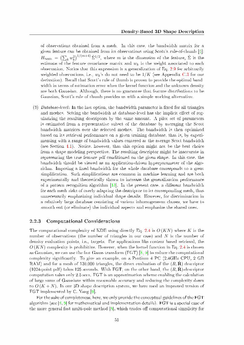
Density-Based 3D Shape Description
of observations obtained from a mesh. In this case, the bandwidth matrix for agiven feature can be obtained from its observations using Scott's rule-of-thumb [6]:
HScott =(∑
k w2k
)1/(m+4) Σ1/2, where m is the dimension of the feature, Σ is theestimate of the feature covariance matrix and wk is the weight associated to eachobservation. Notice that this expression is a generalization of Eq. 2.9 for arbitrarilyweighted observations, i.e., wk's do not need to be 1/K (see Appendix C.3 for ourderivation). Recall that Scott's rule-of-thumb is proven to provide the optimal band-width in terms of estimation error when the kernel function and the unknown densityare both Gaussian. Although, there is no guarantee that feature distributions to beGaussian, Scott's rule-of-thumb provides us with a simple working alternative.
(3) Database-level : In the last option, the bandwidth parameter is xed for all trianglesand meshes. Setting the bandwidth at database-level has the implicit eect of reg-ularizing the resulting descriptors by the same amount. A pilot set of parametersis estimated from a representative subset of the database by averaging the Scottbandwidth matrices over the selected meshes. The bandwidth is then optimizedbased on its retrieval performance on a given training database, that is, by experi-menting with a range of bandwidth values centered at the average Scott bandwidth(see Section 4.1). Notice, however, that this option might not be the best choicefrom a shape modeling perspective. The resulting descriptor might be inaccurate inrepresenting the true feature pdf conditioned on the given shape. In this case, thebandwidth should be viewed as an application-driven hyperparameter of the algo-rithm. Imposing a xed bandwidth for the whole database corresponds to a greatsimplication. Such simplications are common in machine learning and are bothexperimentally and theoretically shown to increase the generalization performanceof a pattern recognition algorithm [13]. In the present case, a dierent bandwidthfor each mesh risks of overly adapting the descriptor to its corresponding mesh, thusunnecessarily emphasizing individual shape details. However, for discrimination ina relatively large database consisting of various inhomogeneous classes, we have tosmooth out (or eliminate) the individual aspects and emphasize the shared ones.
2.2.3 Computational Considerations
The computational complexity of KDE using directly Eq. 2.4 is O (KN) where K is thenumber of observations (the number of triangles in our case) and N is the number ofdensity evaluation points, i.e., targets. For applications like content-based retrieval, theO (KN)-complexity is prohibitive. However, when the kernel function in Eq. 2.4 is chosenas Gaussian, we can use the fast Gauss transform (FGT) [8, 9] to reduce the computationalcomplexity signicantly. To give an example, on a Pentium 4 PC (2.4GHz CPU, 2 GBRAM) and for a mesh of 130,000 triangles, the direct evaluation of the (R, R)-descriptor(1024-point pdf) takes 125 seconds. With FGT, on the other hand, the (R, R)-descriptorcomputation takes only 2.5 secs. FGT is an approximation scheme enabling the calculationof large sums of Gaussians within reasonable accuracy and reducing the complexity downto O (K + N). In our 3D shape description system, we have used an improved version ofFGT implemented by C. Yang [9].
For the sake of completeness, here, we only provide the conceptual guidelines of the FGTalgorithm (see [8, 9] for mathematical and implementation details). FGT is a special case ofthe more general fast multi-pole method [8], which trades o computational simplicity for
51

2.3 Descriptor Manipulation Tools
acceptable loss of accuracy. The basic idea is to cluster the source points and target pointsusing appropriate data structures and to replace the large sums with smaller ones thatare equivalent up to a given precision. The gain in complexity is achieved by avoiding thecomputation of every Gaussian at every evaluation point unlike the direct approach, whichhas O (KN)-complexity. Instead, truncated Hermite series (each of which is equivalent toan exponential in the sum) are constructed about a small number of source cluster-centersin O (K) operations. The accuracy can be controlled by the truncation order. Theseseries are then shifted to target cluster-centers, and evaluated at the K targets in O (N)operations. Basically, since the two sets of operations are disjoint, the total complexity ofFGT becomes O (K + N).
2.3 Descriptor Manipulation Tools
2.3.1 Marginalization
Features can be selectively removed from the multivariate pdf-based descriptor by mar-ginalization, that is, by integrating out feature variables. Specically, to remove the com-ponent Si from the pdf of some m-dimensional feature S = (S1, . . . , Si, . . . , Sm), we usethe following equation:
fS 6i|O , fS 6i (s1, . . . , si−1, si+1, . . . , sm|O) , (2.11)
=∫
Si
fS (s1, . . . , si, . . . , sm|O) dsi, (2.12)
which gives the pdf of a reduced feature S 6i , (S1, . . . , Si−1, Si+1, . . . , Sm). Reducingthe descriptor fS|O to fS 6i|O saves us one dimension at the cost of losing any informationbrought by the component Si. For instance, marginalizing the magnitude component Rfrom the pdf of (R, R)-feature vector, the size of the descriptor f( 6R,R)|O is NR times smaller
than that of f(R,R)|O since the target set for (R, R) contains NR×NR points. We can thenhope to identify features that can be marginalized for the sake of dimensionality reduction,while monitoring the descriptor's discrimination ability. An obvious instance is the caseof a redundant component in the directional parts R and N of the local features (R, R)and (D, N) respectively. For example, R is unit norm with R2
x + R2y + R2
z = 1, hence givenany two components, say Rx and Ry, the third one Rz is completely determined up to thesign. Thus, it can be conjectured that Rz can be marginalized out without deterioratingperformance. We show this experimentally in Section 4.5.1.
Marginalization is an appealing tool, which can be used for more interesting tasks thandimensionality reduction. In the introduction of this chapter and in Section 2.1.1, we havepointed out that our framework can produce a family of descriptors using dierent sets ofmultivariate features. The specicity of a feature increases as a function of the includedcomponents, hence, in principle, the corresponding pdf-based descriptor should becomemore discriminating as more components are added. The critical issue is to determine howmuch the feature is to be specic, or equivalently, which components are to be included inthe nal multivariate feature to obtain the best performance for a particular classicationand/or retrieval task. This problem can be viewed as a particular instance of featureselection, for which many suboptimal heuristics have been developed [86]. Given L dierentfeatures and |O| objects, a naive solution is to construct all 2L − 1 feature combinationsand then to calculate 2L − 1 sets of |O| pdf-based descriptors for subsequent performance
52

Density-Based 3D Shape Description
Figure 2.8: Illustration of probability density pruning on a univariate example
evaluation. Using marginalization, we can avoid this laborious descriptor computationphase by computing just one set of descriptors, without resorting to any heuristics. Thisone set of descriptors corresponds to the case in which all of the L features are included.We can then invoke the marginalization equation (Eq. 2.12) to obtain the descriptorscorresponding to all subsets of the L features. Evidently, this procedure is exact (withinpdf estimation accuracy) and way more ecient than the naive solution. We employ thisparticular facet of marginalization in Section 4.6.2.
2.3.2 Probability Density Pruning
Another approach to reduce a descriptor's dimensionality involves identifying insignicanttargets (density evaluation points) by pruning the prior feature density, dened in Eq. 2.3.This idea is eected as follows. For a selected threshold λ, we dene a new target setRλ
S = tn ∈ RS : fS(tn) > λ (see Figure 2.8). The reduced descriptor for some object Obecomes then fλ
S|O = [fS(tn|O)]tn∈R
λS. In other words, we eliminate the targets at which
prior density values are below the threshold λ. We conjecture that these targets are notsignicant in describing the shapes as they do not induce large pdf values on average,hence they can be pruned from the descriptors. Notice that heuristic selection methodsare not practical when the descriptor vector size is in the order of thousands. Pruning bysuppressing small pdf values, albeit not tantamount to feature selection, still serves thegoal by reducing the descriptor size. Note also that once insignicant target points areeliminated by pruning, we can use the new target set Rλ
S for KDE. RλS having smaller
cardinality than the original RS , we can also save from descriptor computation time.
53

2.4 An Invariant Similarity Measure for Pdfs
2.4 An Invariant Similarity Measure for Pdfs
In this section, we deliver an important result on recovering invariance against certain typesof object transformations at the matching stage. We start by recalling the rule relatingtwo pdfs under transformations of random variables. Consider a generic random variableS ∈ RS with pdf fS . Let Γ be a bijection on RS . The pdf of S is related to the pdf of itstransformed version Γ(S) by
fS(s) = fΓ(S)(Γ(s))|JΓ(s)|, (2.13)
where JΓ is the Jacobian of Γ. Recall that the Jacobian of a transformation Γ is thedeterminant of the matrix of its rst partial derivatives.
The above identity may have several applications in our context. For instance, considerthe situation where we have a 3D object O embedded in a certain reference frame F andwe dispose of the pdf fS|O , fS(·|O) of a pose-dependent feature S evaluated on the
surface of this object. The radial direction feature R and the normal feature N can betwo such features. Suppose furthermore that we observe the same object O but in adierent reference frame F′. Let the transformation Γ be the mapping from F and F′,that is, applying Γ on O in F, we can obtain O in F′. In this specic case, Γ is anorthogonal transformation, accounting for rotations, relabelings, and mirror reections ofthe coordinate axes. Clearly, applying Γ on the object O does not change its intrinsicshape properties neither the shape information contained in the feature S. The sole eectof this transformation is to map S, evaluated in F, to Γ(S) evaluated in F′. By Eq. 2.13and the fact that |JΓ(s)| = |Γ| = 1,∀s ∈ RS , in this specic case, we can relate the pdfsfS|O and fΓ(S)|O of the feature S, evaluated when the object O is in F and F′ respectively,by the following identity
fS(s|O) = fΓ(S)(Γ(s)|O),∀s ∈ RS . (2.14)
The problem of recovering the pose of an object O in F′ with respect to F boils down tonding Γ that satises the identity in Eq. 2.14. In principle, we can solve this problem byinvoking a distance measure between fS|O and fΓ(S)|O such as the L1-distance and settingit to zero: ∫
s∈RS
∣∣fS(s|O)− fΓ(S)(Γ(s)|O)∣∣ds = 0. (2.15)
Whenever the pdfs fS|O and fΓ(S)|O are available, Eq. 2.15 can be solved with respect toΓ, either numerically or analytically.
Guided by the above discussion, we can dene a similarity2 measure between twodierent objects O and O′ as follows:
dist(O,O′) = minΓ∈O(3)
∫s∈RS
∣∣fS(s|O)− fΓ(S)(Γ(s)|O′)∣∣ds, (2.16)
where O(3) is the group of orthogonal transformations in R3. This measure is invariantagainst the extrinsic eects of rotations, relabelings and mirror reections of the coordinateaxes and captures solely intrinsic shape variations to the extent encoded by the featurepdfs.
Let us now explain how and in which situations we can implement this measure fordensity-based descriptors. Observe that Eq. 2.16 is quite implicit and assumes that the pdfs
2Actually a dissimilarity measure.
54

Density-Based 3D Shape Description
are analytically available and continuous. Recall, however, that a density-based descriptoris just a discretized version of the continuous pdf, i.e., it is a nite vector given by fS|O =[fS(t1|O), . . . , fS(tN |O)] for the object O and fS|O′ = [fS(t1|O′), . . . , fS(tN |O′)] for the
object O′. Recall also that the set RS = tn ∈ RSNn=1 is the target set at which the pdf
is evaluated. With this notation, the discretized version of the measure in Eq. 2.16 wouldbe
dist(O,O′) = minΓ∈O(3)
∥∥fS|O − fΓ(S)|O′∥∥
L1 (2.17)
= minΓ∈O(3)
N∑n=1
∣∣fS(tn|O)− fΓ(S)(Γ(tn)|O′)∣∣, (2.18)
provided that RS is a uniform partitioning of RS (cf. Section 2.1.3). There remainsone important problem regarding the calculation of this measure. To perform the min-imization in ( 2.17) with respect to Γ, we need the pdf values fΓ(S)(Γ(tn)|O′) but weonly have fS(tn|O′). Hopefully, whenever RS is closed under the action of Γ (i.e., when∀t ∈ RS ,Γ(t) = t′ ∈ RS), Γ maps the target t to t′, which is also in the target set. ByEq. 2.14, we have fS(t|O′) = fΓ(S)(t′|O′). Thus, given the descriptor fS|O′ and a certainΓ, we can recover fΓ(S)|O′ by just permuting the vector entries, without re-evaluating thedescriptor for every admissible Γ. Evaluation of Eq. 2.17 becomes a matter of testingadmissible transformations Γ (under the action of which the target set RS is closed) andpicking the minimum value.
The set of admissible transformations Γ needs further attention as it determines thetype of invariances we want to achieve at the matching stage. In Eqs. 2.16 and 2.17, thisset is specied as the group of orthogonal transformations O(3), which includes rotations,relabelings and mirror reections of the coordinate axes. From a practical viewpoint,the minimization involved in the discrete case of Eq. 2.17 can only be performed by anexhaustive search on the set of admissible Γ. Thus, the cardinality of the search spacematters a lot in order to obtain a measure that can be computed within reasonable time.Accordingly, we focus on developing a similarity measure invariant to relabelings and mirrorreections (but not to rotations) due to following reasons:
• Rotations form a subgroup of O(3), and are called as special orthogonal transfor-mations SO(3), which contains innitely many Γ. Thus in the continuous case ofEq. 2.16, the minimization is to be performed within an innite set. In the discretecase that we are particularly concerned with, the cardinality of the search space de-pends on the granularity of the target set, that is, how ne RS is partitioned intoRS . The larger the target set is, the larger the set of admissible rotations becomes.On the other hand, the set of admissible axis relabelings and mirror reections in R3,denoted by PS(3), has nite cardinality both in the continuous and discrete cases.A labeling means which one of the three coordinate axes is the x-axis, which one isthe y-axis and which one is the z-axis. A mirror reection changes their polarity.The three axes of the 3D coordinate system can be labeled in 3! = 6 possible ways.Given a certain labeling, there are 23 = 8 possible polarity assignments. Thus, thereare 6× 8 = 48 possible xyz-congurations. The passage from one axis congurationto another can be eected with a matrix Γ, which consists of the product of a per-mutation matrix (for relabelings) and a sign matrix (for reections), as illustrated inFigure 2.9.
55

2.4 An Invariant Similarity Measure for Pdfs
Figure 2.9: A permutation P followed by a polarity reversal S changes the axis congura-tion form F to F′.
• In descriptor-based 3D retrieval, rotation errors constitute a lesser problem thanmislabelings or wrong polarity assignments of the coordinate axes. In general, PCA-based object normalization methods correctly nd the major axes of the 3D objectbut fail to unambiguously resolve the labels and/or the polarities of these axes (seeFigure 2.10) [87]. After normalization, rotation errors remain in small amount sothat the variation between descriptors becomes unimportant, or not that much sig-nicant as a mislabeling or a wrong polarity assignment would produce. Furthermore,smoothness reinforced by the KDE-based scheme can gloss over small rotation errors,as discussed in Section 2.2.1.
Figure 2.10: Three airplane models after pose normalization: major axes are correctlyfound but the front of the fuselage of the rightmost model is in the opposite direction.
The importance of target selection reappears since the target set RS should be closedunder the action of Γ ∈ PS(3). Our working example can be pose-dependent features suchas R or N, taking values within the unit 2-sphere S2. In this case, the target set RR
56
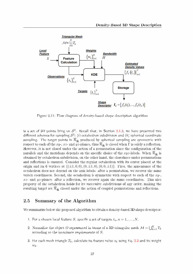
Density-Based 3D Shape Description
Figure 2.11: Flow diagram of density-based shape description algorithm
is a set of 3D points lying on S2. Recall that, in Section 2.1.3, we have presented twodierent schemes for sampling S2: (i) octahedron subdivision and (ii) spherical coordinatesampling. The target points in RR produced by spherical sampling are symmetric withrespect to each of the xy-, xz- and yz-planes, thusRR is closed when Γ is solely a reection.However, it is not closed under the action of a permutation since the conguration of theparallels and the meridians depends on the specic choice of the xyz-labels. When RR isobtained by octahedron subdivision, on the other hand, the closedness under permutationsand reections is ensured. Consider the regular octahedron with its center placed at theorigin and its 6 vertices at (±1, 0, 0), (0,±1, 0), (0, 0,±1). First, the appearance of theoctahedron does not depend on the axis labels: after a permutation, we recover the samevertex coordinates. Second, the octahedron is symmetric with respect to each of the xy-,xz- and yz-planes: after a reection, we recover again the same coordinates. This niceproperty of the octahedron holds for its successive subdivisions of any order, making theresulting target set RR closed under the action of coupled permutations and reections.
2.5 Summary of the Algorithm
We summarize below the proposed algorithm to obtain a density-based 3D shape descriptor:
1. For a chosen local feature S, specify a set of targets tn, n = 1, . . . , N .
2. Normalize the object O represented in terms of a 3D triangular mesh M =⋃K
k=1 Tk
according to the invariance requirements of S.
3. For each mesh triangle Tk, calculate its feature value sk using Eq. 2.2 and its weightwk.
57

2.5 Summary of the Algorithm
4. Set the bandwidth parameters Hk according to the strategy chosen among the threeoptions described in Section 2.2.2.
5. For each target tn, n = 1, . . . , N , evaluate the feature pdf fS (tn|O), using Eq. 2.5.
6. Store the resulting density values fS (tn|O) in the shape descriptorfS|O = [fS (t1|O) , . . . , fS (tN |O)].
7. If necessary, marginalize and/or prune the descriptor to reduce dimensionality, asdescribed in Section 2.3.
Figure 2.11 depicts the ow diagram of the algorithm when the bandwidth parametersare set at database-level. Alternatively, in the triangle or mesh-level setting, a bandwidthmatrix is to be computed for each triangle or for the entire mesh, respectively. Note thatin Figure 2.11, we assume that the mesh M has already undergone a pose and/or scalenormalization step depending on the missing invariance properties of the local feature Schosen.
58

Chapter 3
Statistical Similarity Learning
Ongoing research in 3D shape retrieval shows that no single descriptor is capable of pro-viding satisfactory retrieval performance for a broad class of shape databases, regardlessof the associated semantics [2, 23, 3]. Figure 3.1 displays the response of two dierentdescriptors A and B to two dierent queries from the Princeton Shape Benchmark [23].The rst query is a biplane model and the second one is a chair model. In response tothe biplane model, descriptor A returns correctly four biplanes in the rst three and inthe sixth matches, while the fourth and the fth retrieved models are not biplanes, butstill ying objects that can be considered as relevant. Descriptor B, on the other hand,returns models that are completely irrelevant to the biplane query (three shelf models,two coarse human models and a microscope!). For the chair query, the situation revertsto the advantage of Descriptor B, which can retrieve six chair models; while descriptorA, after rst three correct matches, returns two tree models and a monument! Thus, theadequacy of the descriptors A and B depends on the nature of the query. Furthermore,these examples can be multiplied; for instance, there are cases where the sets of relevantmatches for dierent descriptors are disjoint (see Figure 3.2). This suggests that a goodretrieval machine should rely on a diverse set of descriptors for robust performance.
As the example in Figure 3.1 illustrates, experimental evidence motivates us to considerfusion schemes to learn similarities between pairs of objects on statistical grounds. Inthe present chapter, we tackle the similarity learning problem by a score fusion scheme,which minimizes a convex regularized version of the empirical risk associated with rankinginstances. We follow the statistical learning framework developed in [10, 11] and providean application to 3D shape retrieval. We observe that learning a linear scoring function canbe cast into binary classication in the score dierence domain, that is, nding a separatinghyperplane. Given a query, the hyperplane parameters can be considered as optimal withrespect to the empirical risk associated with ranking instances.
Our approach can be contrasted to the one in [88] where the ranking problem is for-mulated as classication of pairwise instances using dierence vectors (between descriptorsin our setting) inputted to an SVM-type algorithm. Our solution diers from that of [88]in that it operates on scores rather than on the specic representations associated withtraining instances. We prefer to work with scores due to following reasons:
• Even though most of the 3D shape descriptors proposed in the literature [2, 3] arevector-based, the computation of non-classical similarity measures involves a mini-mization over a set of plausible transformations in order to secure invariance againstcertain types of transformations (cf. Section 2.4). As exemplied in Section 2.4,
59

Figure 3.1: Response of two dierent descriptors A and B to two dierent queries biplaneand chair
such procedures may require permutations of descriptor vector entries, in which case,working with descriptors rather than with scores would become very hard, if not im-possible.
• On a more general vein, descriptors might not be vectors but graphs with specializedmetrics for matching. Consequently, working with scores makes our approach a moregeneral solution to statistical similarity learning.
• In the 3D shape retrieval domain, descriptor dimensionality can easily reach theorder of thousands. Combining scores has this additional benet of reducing datadimensionality in an informed way.
There is a considerable body of work concerning statistical ranking, which nd appli-cation niches in other than the 3D shape retrieval, such as text-based information retrievaland collaborative ltering. Large margin approaches as in [88, 89] considered the problemas one of ordinal regression, in which case relevance labels are treated as categorical vari-ables at ordinal scale. In these approaches, the aim is to nd a set of rank boundaries inthe feature domain. In [90], the authors adapted the on-line perceptron learning schemeto the ranking problem to cope with situations where training examples are not readilyavailable prior to learning. On a dierent spirit, the works in [91, 92] treated the problemas combining preference judgments based on a variation of the AdaBoost algorithm forbinary classication. Recently in [93], the authors proposed a computationally ecientapproximation for learning a ranking function from structured order constraints on sets oftraining samples.
This chapter is organized as follows. In Section 3.1, we introduce the score fusionproblem as well as the notation that we will use subsequently. In Section 3.2, following
60

Statistical Similarity Learning
Figure 3.2: Response of two dierent descriptors A and B to the same query: both de-scriptors retrieve dierent plausible matches.
[11], we recapitulate the ranking risk minimization framework. In Section 3.3, we givean SVM-based solution to the score fusion problem. Finally, in Section 3.4, we proposedierent search protocols for the retrieval machine combining multiple sources of similarityinformation.
3.1 The Score Fusion Problem
In this section, we introduce the score fusion problem for 3D shape retrieval following thestatistical ranking framework developed in [10, 11]. Consider the problem of ranking twogeneric database shapes x and x′ based on their relevance to a query shape q. Supposethat we have access to K similarity values simk(x, q) , sk and simk(x′, q) , s′k for eachof the pairs (x, q) and (x′, q) respectively, where k = 1, . . . ,K. In our context, each simi-larity value sk arises from a dierent shape descriptor and reects some, possibly dierent,geometrical and/or topological commonality of shape pairs (x, q) and (x, q′). For simi-lar shape pairs, an ideal similarity value should be higher than it is for less similar ones.In retrieval problems, a shape x in the database that is more similar to the query q isexpected to be ranked higher than another intrinsically less similar shape x′. These simi-larity values/scores can be written more compactly in the vector form as s = [s1, . . . , sK ]and s′ = [s′1, . . . , s
′K ] where s, s′ ∈ RK . Our objective is to build a scalar-valued scoring
function ϕ of the form ϕ(x, q) = 〈w, s〉, where w = [w1, . . . , wK ] ∈ RK is a vector, whosecomponents are associated with the individual scores sk. The scoring function ϕ shouldassign a higher score to the shape, which is more relevant to the query q, i.e., it shouldsatisfy the following property:
ϕ(x, q) > ϕ(x′, q) if x is more relevant to q than x′,ϕ(x, q) < ϕ(x′, q) otherwise,
where ties are arbitrarily broken. The relevance of the shapes x and x′ to the query qcan be encoded by indicator variables y and y′ respectively. In this work, we assume crisprelevances y = 1 (relevant) and y = −1 (not relevant), in which case, the above propertyreads as:
ϕ(x, q) > ϕ(x′, q) if y − y′ > 0,ϕ(x, q) < ϕ(x′, q) if y − y′ < 0.
61

3.2 Ranking Risk Minimization
The function ϕ must subsume the similarity information residing in the individualscores sk in order to emulate the ideal similarity notion between shapes, hence to achievea better retrieval performance. Given the linear form ϕ(x, q) = 〈w, s〉, score fusion canbe formulated as the problem of nding an optimal weight vector w, according to somecriterion, as we explain in the following section.
3.2 Ranking Risk Minimization
The criterion of interest is the so-called ranking risk dened as
R(ϕ; q) = P((ϕ(x, q)− ϕ(x′, q)) · (y − y′) < 0
).
In other words, the ranking risk with respect to the query q is the probability that ϕ givesa score for x higher than it gives to x′ while x′ is relevant to q but x is not. Naturally, wewant this probability to be as small as possible. Rewriting the misranking probability interms of an expectation, we have
P((ϕ(x, q)− ϕ(x′, q)) · (y − y′) < 0
)= E
I(ϕ(x, q)− ϕ(x′, q)) · (y − y′) < 0
,
where I· is one if the predicate inside the braces is true and zero otherwise. Since wedo not have access to the probability measure P on (x, y), we have to nd an empiricalestimate of the ranking risk based on a training set X = (xn, yn)N
n=1. A natural estimatefor this expectation can be obtained by averaging over the pairwise instances of the trainingset X [10, 11], i.e.,
R(ϕ; q) =2
N(N − 1)
∑m<n
I (ϕ(xm, q)− ϕ(xn, q)) · (ym − yn) < 0 . (3.1)
The properties of this empirical quantity, known as a U -statistic in the statistics liter-ature, has been investigated in the context of statistical ranking [10, 11]. This particulartype of risk functional uses the 0-1 loss to assess the cost of a misranked pair of objects,i.e., if ϕ(xm, q) < ϕ(xn, q) and ym > yn, the scoring function ϕ(·, q) (wrongly) assigns ahigher score to xn than to xm while xm is relevant to the query q but xn is not. Thusthe scoring function has made an error in ranking xn and xm with respect to the query q.Such misrankings are naturally undesirable and our task is to nd a scoring function (ormore appropriately its parameters w) so that the number of misranked pairs is as small aspossible.
3.3 SVM Formulation
We can identify the empirical ranking risk in Eq. 3.1 as an empirical classication error.Let z , (y − y′)/2, taking values within −1, 0, 1. We observe then the following:
z =
1 x should be ranked higher than x′,−1 x should be ranked lower than x′.
When z = 0, i.e., if shapes x and x′ are both relevant (y = y′ = 1) or both not relevant(y = y′ = −1), we have no particular preference in ranking them with respect to eachother (we can decide arbitrarily). Corresponding to each non-zero z, we can dene a score
62
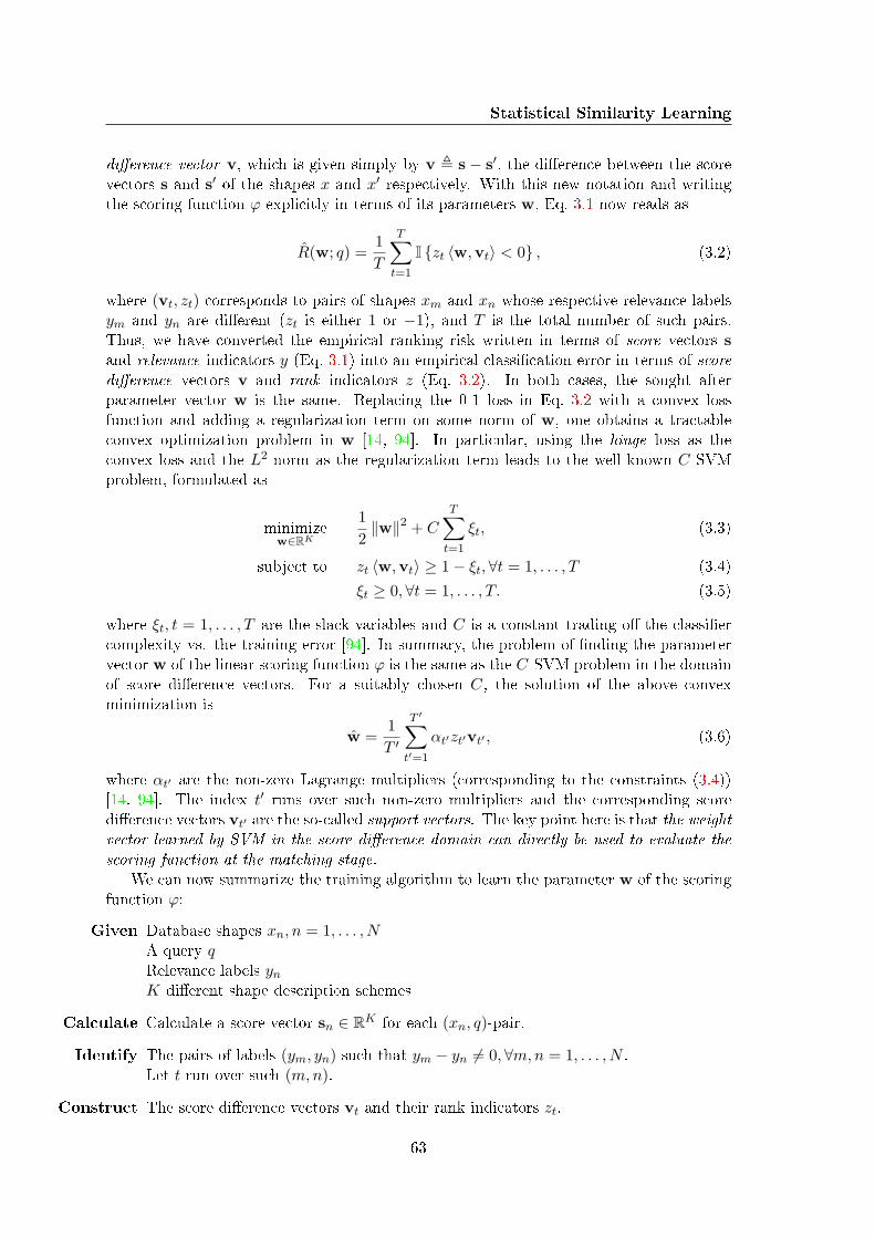
Statistical Similarity Learning
dierence vector v, which is given simply by v , s − s′, the dierence between the scorevectors s and s′ of the shapes x and x′ respectively. With this new notation and writingthe scoring function ϕ explicitly in terms of its parameters w, Eq. 3.1 now reads as
R(w; q) =1T
T∑t=1
I zt 〈w,vt〉 < 0 , (3.2)
where (vt, zt) corresponds to pairs of shapes xm and xn whose respective relevance labelsym and yn are dierent (zt is either 1 or −1), and T is the total number of such pairs.Thus, we have converted the empirical ranking risk written in terms of score vectors sand relevance indicators y (Eq. 3.1) into an empirical classication error in terms of scoredierence vectors v and rank indicators z (Eq. 3.2). In both cases, the sought afterparameter vector w is the same. Replacing the 0-1 loss in Eq. 3.2 with a convex lossfunction and adding a regularization term on some norm of w, one obtains a tractableconvex optimization problem in w [14, 94]. In particular, using the hinge loss as theconvex loss and the L2-norm as the regularization term leads to the well-known C-SVMproblem, formulated as
minimizew∈RK
12‖w‖2 + C
T∑t=1
ξt, (3.3)
subject to zt 〈w,vt〉 ≥ 1− ξt,∀t = 1, . . . , T (3.4)
ξt ≥ 0,∀t = 1, . . . , T. (3.5)
where ξt, t = 1, . . . , T are the slack variables and C is a constant trading o the classiercomplexity vs. the training error [94]. In summary, the problem of nding the parametervector w of the linear scoring function ϕ is the same as the C-SVM problem in the domainof score dierence vectors. For a suitably chosen C, the solution of the above convexminimization is
w =1T ′
T ′∑t′=1
αt′zt′vt′ , (3.6)
where αt′ are the non-zero Lagrange multipliers (corresponding to the constraints (3.4))[14, 94]. The index t′ runs over such non-zero multipliers and the corresponding scoredierence vectors vt′ are the so-called support vectors. The key point here is that the weightvector learned by SVM in the score dierence domain can directly be used to evaluate thescoring function at the matching stage.
We can now summarize the training algorithm to learn the parameter w of the scoringfunction ϕ:
Given Database shapes xn, n = 1, . . . , NA query qRelevance labels yn
K dierent shape description schemes
Calculate Calculate a score vector sn ∈ RK for each (xn, q)-pair.
Identify The pairs of labels (ym, yn) such that ym − yn 6= 0,∀m,n = 1, . . . , N .Let t run over such (m,n).
Construct The score dierence vectors vt and their rank indicators zt.
63

3.4 Applications
Run The C-SVM algorithm to learn the weight vector w ∈ RK ,using the set (vt, zt)T
t=1 ⊂ RK × −1, 1.
3.4 Applications
In this section, we illustrate our score fusion scheme for similarity learning in two dierentretrieval protocols: (i) bimodal search and (ii) two-round search.
3.4.1 Bimodal Search
In this scenario, the user provides a textual description associated with the query shape.The keyword can be selected from one of the predened class concepts. We call thisprotocol as bimodal since the query is formulated in terms of two information modalities, a3D shape and a concept keyword. This protocol necessitates an o-line stage during whichthe weight vectors associated with each class concept are learned. Note that the criterionthat we have elaborated on in the previous sections is per-query and should be extendedto a per-concept risk R(w, C), where C stands for the working concept. This can be donestraight-forwardly by averaging per-query risks associated with a given concept, that is,
R(w; C) =1|C|∑q∈C
R(w; q), (3.7)
where |C| is the number of training shapes belonging to C. However, since the minimizationshould be performed in the score dierence domain, the problem turns out to be a verylarge-scale one even for moderately sized classes. Given a training database D of size |D|,the number of score dierence instances per concept is |C| × (|C| − 1) × (|D| − |C|), e.g.,for |D| = 1000 and for |C| = 10, the number of training instances becomes ∼ 90000, inwhich case we incur to memory problems using standard SVM packages [95]. In order tomaintain the generality and practical usability of our approach in this protocol, we developtwo heuristics:
(1) Average per-query weight vector. The weight vector wC for a given conceptclass is computed as the average of the per-query weight vectors corresponding tothe training models within that class, that is,
wC =1|C|∑q∈C
wq (3.8)
where wq is the weight vector for query q, obtained by minimizing the convex regu-larized version of Eq. 3.2. We denote this heuristic by AVE-W.
(2) Per-class risk minimization using per-query support vectors. In this secondheuristic, we exploit the sparsity of the SVM solution, which means that the per-query weight vector given in Eq. 3.6 is the weighted sum of usually a much smallernumber of training instances than the size of the whole training set. It is a wellknown fact that, for a given problem, the SVM solution remains the same when onlythe support vectors are provided for minimization [14, 94]. By this token, supportvectors can also be called as dicult instances" of the training problem. They reectthe distribution of training data in an economical way, as they are fewer in numberthan the whole training instances. Accordingly, the learning of a per-concept weight
64

Statistical Similarity Learning
vector can be carried in two stages. First, we identify the support vectors of per-query problems by per-query minimization. Then, we pool all the support vectorscorresponding to a given concept and perform the minimization using this newlyformed set to learn the per-concept weight vector. We repeat this procedure asmany times as the number of predened shape concepts. We denote this heuristicby PCMIN-W.
3.4.2 Two-round Search
This protocol requires user intervention during the querying process. In the rst round,the retrieval machine returns a ranked list of shapes using a simple scoring scheme, e.g.,the sum of the available raw scores. After the rst found, we can invoke the score fusionscheme in two dierent ways:
(1) On-line. The user marks M models among the returned ones, as either relevant(y = 1) or non-relevant (y = −1) with respect to his/her query. In the secondround, the retrieval machine returns a rened ranked list using the scoring functionϕw(x, q) = 〈w, s〉. The weight vector w is learned on-line using the M markedshapes as training instances. In order not to demand too much from the user, Mshould not be large and is typically limited to a few rst instances. For example,when M = 8 and the number of positive M+ and negative instances M− are equal(M+ = M− = 4), the total number of training score dierence vectors is just 16.Consequently, on-line learning is computationally feasible.
(2) O-line. In this variant of the two-round search, all the shapes in the database havetheir individual weight vectors stored, which have already been learned o-line. Theindividual weight vectors can be obtained as in the bimodal protocol. At queryingtime, the user is asked to mark just the rst relevant item in the displayed page ofthe results. The second round evaluates the scoring function ϕw(x, q) = 〈w, s〉 usingthe weight vector corresponding to the marked shape. Clearly, this protocol doesnot perform any on-line learning and constitutes a less demanding option than theformer in terms of user interaction needed, as the user is asked to mark just one item.
The two variants of the two-round protocol presented here constitute particular formsof relevance feedback and prove to be more suitable applications for our similarity learningscheme than bimodal search, as the experiments in Section 4.10 demonstrate.
65

66

Chapter 4
Experiments
In this chapter, we concretize the density-based shape description framework and the scorefusion based similarity learning approach in experimental terms. Our analysis extends overten dierent sections clustered into the following groups:
• Parameter Selection and Robustness Experiments. Bandwidth parameterselection constitutes the major issue in all applications based on KDE. As a startingpoint, in Section 4.1, we experiment with possible bandwidth selection strategiesintroduced for 3D shape description (cf. Section 2.2.2), since the results of all thesubsequent analyses rely upon the bandwidth parameter. In Section 4.2, we illustratethe robustness properties of the density-based framework with an emphasis on theeect of the bandwidth in conjunction with the discussion in Section 2.2.1 on KDEin context.
• Eciency Experiments. We treat the eciency problem as a matter of descriptorparsimony. Target selection experiments in Section 4.3 deal with feature domainsampling, as well as with descriptor size. In Section 4.5, we experiment with ourmarginalization and probability density pruning tools for descriptor dimensionalityreduction. We also compare our ndings with those of the classical PCA approach.
• Eectiveness Experiments. Eectiveness refers to the discrimination ability ofthe descriptors in a retrieval application. In Section 4.4, we show how the invariantmatching scheme introduced in Section 2.4 outperforms standard similarity measures.Sections 4.6 and 4.7 invoke feature-level and score-level information fusion to furtherimprove the retrieval performance of the density-based framework.
• Comparison Experiments. Quite many shape descriptors in the literature haveanalogies to cases of the density-based framework in the local surface features theyuse. Our approach diers from these, which we denominate collectively as histogram-based, in the use of KDE, in which case multivariate extensions come naturally andprove to be more descriptive for the retrieval task as shown in Section 4.8. We alsocompare our scheme against its state-of-the-art competitors. In another comparisonstudy in Section 4.9, we analyze the performance variation of our descriptors acrossdatabases diering in classication properties, class cardinalities and mesh qualities.These databases are (see also Section 1.2):
Princeton Shape Benchmark (PSB) [23]. 1814 general-purpose low-quality 3Dmodels split into two subsets: Training (907 models in 90 classes) and Test
67

(907 models in 92 classes). Classication is induced by functionality as wellas by form. In general, the meshes in PSB have low resolution, they are non-regular, non-smooth and disturbed with degeneracies such as non-manifold, non-connected triangles of varying size and shape. These models are usually calledas triangular soups".
Sculpteur (SCU) [24, 25]. 513 high-quality 3D models in 53 classes consistinglargely of archaeological models. The meshes in SCU are regular, smooth andhighly detailed in terms of resolution.
SHREC Watertight (SHREC-W) [26]. 400 high-quality 3D models in 20 classes.The specialty of this database is that the classication assumes topologicalequivalences in addition to geometrical, constituting a challenging test envi-ronment for geometry-induced description methods. The meshes in SHREC-Ware regular and smooth.
Purdue Engineering Shape Benchmark (ESB) [27]. 865 3D models of engineeringparts in 45 classes. The meshes in ESB are regular but in general non-smoothdue to the general platonic solid form of the engineering parts.
• Statistical Score Fusion Experiments. This last cluster addresses the similaritylearning algorithm for retrieval (Section 4.10). We test the bimodal and two-roundsearch protocols introduced in Chapter 3 and show that more eective 3D retrievalis possible when a moderate amount of supervision is incorporated into the queryingprocess.
We mostly experiment with PSB and to a lesser extent with SCU. Nevertheless, theextensive Section 4.9 reects the virtues of our approach on SHREC-W and ESB. Beforeproceeding with the forthcoming sections, we need to make a clarication on object nor-malization. The local surface features presented in Section 2.1.1 have dierent invarianceproperties. Consequently, whenever a certain feature is invariant to one of the so-calledextrinsic eects such as translation, rotation, mirror reection and isotropic rescaling, the3D object should be normalized prior to descriptor extraction. In our experiments, we hadto carry out the following normalization steps:
• Translation. The object's center of mass is considered as the origin of the 3Dcoordinate system. We calculate the center of mass as the area-weighted average ofthe triangle barycenters.
• Rotation. To nd the three axes of the coordinate system, we use Vranic's contin-uous" PCA approach, where the covariance matrix of the surface points is evaluatedby integrating over triangles instead of mere area-weighted averaging [17]. The ma-jor axes are then found, as is the standard practice, by an eigendecomposition ofthe estimated covariance matrix. The x, y, z labels of the axes are assigned in thedecreasing order of the eigenvalues, while the polarities are estimated by Vranic'smoments-based approach [17]. Note that, with our invariant matching scheme (cf.Section 2.4), we do not need the last two types of normalization, concerning coordi-nate axes relabelings and mirror reections.
• Isotropic Rescaling. We calculate a scale factor as the area-weighted average ofthe surface point-to-origin distances. Dividing the surface point coordinates by thisfactor yields scale normalization.
We hope the reader will enjoy this experimental journey.
68
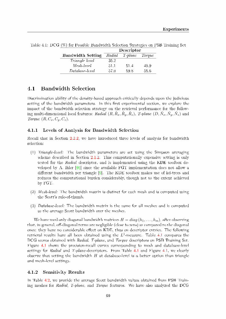
Experiments
Table 4.1: DCG (%) for Possible Bandwidth Selection Strategies on PSB Training SetDescriptor
Bandwidth Setting Radial T-plane TorqueTriangle-level 35.2 - -Mesh-level 51.1 51.4 49.9
Database-level 57.0 59.8 55.6
4.1 Bandwidth Selection
Discrimination ability of the density-based approach critically depends upon the judicioussetting of the bandwidth parameters. In this rst experimental section, we explore theimpact of the bandwidth selection strategy on the retrieval performance for the follow-ing multi-dimensional local features: Radial (R, Rx, Ry, Rz), T-plane (D, Nx, Ny, Nz) andTorque (R,Cx, Cy, Cz).
4.1.1 Levels of Analysis for Bandwidth Selection
Recall that in Section 2.2.2, we have introduced three levels of analysis for bandwidthselection:
(1) Triangle-level: The bandwidth parameters are set using the Simpson averagingscheme described in Section 2.1.2. This computationally expensive setting is onlytested for the Radial descriptor, and is implemented using the KDE toolbox de-veloped by A. Ihler [96] since the available FGT implementation does not allow adierent bandwidth per triangle [9]. The KDE toolbox makes use of kd-trees andreduces the computational burden considerably, though not to the extent achievedby FGT.
(2) Mesh-level: The bandwidth matrix is distinct for each mesh and is computed usingthe Scott's rule-of-thumb.
(3) Database-level: The bandwidth matrix is the same for all meshes and is computedas the average Scott bandwidth over the meshes.
We have used only diagonal bandwidth matrices H = diag (h1, . . . , hm), after observingthat, in general, o-diagonal terms are negligible (close to zero) as compared to the diagonalones: they have no considerable eect on KDE, thus on descriptor entries. The followingretrieval results have all been obtained using the L1-measure. Table 4.1 compares theDCG scores obtained with Radial, T-plane, and Torque descriptors on PSB Training Set.Figure 4.1 shows the precision-recall curves corresponding to mesh and database-levelsettings for Radial and T-plane-descriptors. From Table 4.1 and Figure 4.1, we clearlyobserve that setting the bandwidth H at database-level is a better option than triangleand mesh-level settings.
4.1.2 Sensitivity Results
In Table 4.2, we provide the average Scott bandwidth values obtained from PSB Train-ing meshes for Radial, T-plane, and Torque features. We have also analyzed the DCG
69

4.1 Bandwidth Selection
Figure 4.1: Precision-Recall curves with a bandwidth selection made at mesh-level vs.database-level for the Radial (top) and T-plane (bottom) descriptors on PSB Training Set
performance sensitivity as a function of the database-level bandwidth parameters. Givena database-level Scott bandwidth matrix H, we have carried this analysis by testing theperformance of the descriptors obtained using perturbed bandwidth matrices of the formcH where c is a scalar multiplicative perturbation factor. In Figure 4.2, we provide theDCG prole as a function of c ∈ [0.1, 2.0] with steps of 0.1 for the Radial descriptor. Fromthis prole, we can infer the following:
• Within the c ∈ [0.9, 1.3] interval, the prole remains at at around DCG=57%. Thisshows that, under the database-level assumption, averaging Scott bandwidths is asensible option.
70

Experiments
Table 4.2: Average Scott Bandwidths Obtained from the PSB Training Set: hi, i = 1, . . . , 4corresponds to the ith component of the feature.
Bandwidth Parameters
Descriptor h1 h2 h3 h4
Radial 0.199 0.338 0.226 0.141T-plane 0.202 0.239 0.270 0.285Torque 0.199 0.153 0.236 0.236
Figure 4.2: DCG Performance Sensitivity of the Radial descriptor to bandwidth parameters(see text)
• The performance degrades for small (c ∈ [0.1, 0.9]) and large (c ∈ [1.3, 2.0]) band-width values. Small bandwidth values correspond to under-smoothed pdf estimateswhile large values correspond to over-smoothed estimates (cf. Section 2.2.1).
• The performance degradation for under-smoothed estimates is much steeper thanthe over-smoothed ones. We interpret this as an experimental evidence for the reg-ularization behavior of the KDE-based approach. Under-smoothed estimates reectspecic details about the features, hence descriptors become too much object-specic.Over-smoothed estimates, on the other hand, eliminate such details and emphasizecommonalities between features/shapes. We deduce that the performance is lesssensitive to large bandwidth values than to smaller ones.
The above analysis changes the bandwidth parameters only along a line in the para-meter space. One might wonder about the situation when each average Scott bandwidthvalue is perturbed by its own factor. For each of the four bandwidth values of the Radialdescriptor, we have sampled 100 uniformly distributed values within the at performanceinterval [0.9hi, 1.3hi]. Using the obtained 100 bandwidth four-tuples, we have recomputed100 descriptor sets and tested their performance. The average DCG statistic over these 100
71

4.2 Robustness Results
descriptor sets has been 56.8 ± 0.1%, the maximum and the minimum values being 57%and 56.5%. We deduce that, since the DCG performance persists with very low variation,the Scott bandwidth averaged at database-level constitutes a viable bandwidth selectionoption.
4.2 Robustness Results
4.2.1 Eect of Feature Calculation
The feature observations can be obtained from each mesh triangle, vertex or using theSimpson averaging scheme as presented in Section 2.1.2. In this section, we experimentwith these feature calculation options. For this analysis, we have evaluated the retrievalperformance of the Radial feature on PSB Training Set and SCU. As mentioned in Sec-tion 1.2, PSB meshes contain, in general, a smaller number of triangles of arbitrary sizeand shape, in contrast to highly detailed and regular SCU meshes. In Table 4.3, we providethe DCG performance of the Radial descriptor for each of the feature calculation schemes.These results show that Simpson averaging is more eective than the remaining vertex orcentroid-based options for PSB, while for SCU, all schemes lead to similar performance.Consequently, we recommend Simpson averaging especially for coarse meshes.
Table 4.3: DCG (%) of Radial descriptor using Dierent Feature Calculation Schemes onPSB Training Set and SCU
Databases
Feature Calculation PSB Training SCUVertex 56.0 71.3Centroid 55.6 71.2Simpson 57.0 71.3
4.2.2 Robustness against Low Mesh Resolution
3D models of a certain shape may occur in dierent levels of detail, as in Figure 4.3,where we display meshes representing a unit sphere at various resolutions, from ne tocoarse. Although after a certain level, the mesh might become semantically dierent fromits original version, mesh resolution should not be taken as an intrinsic shape property.Accordingly, we expect that a shape descriptor exhibits small variations against changesin the level of detail. To analyze the behavior of the density-based descriptors undersuch circumstances, we have taken the highest resolution sphere (with 65024 faces) shownin Figure 4.3 and simplied it successively using the quadric edge collapse decimationprocedure built in the MeshLab software [97]. Each decimation halves the number of faces.After simplifying the meshes successively, we have calculated the pdf-based descriptorscorresponding to Radial Distance and Normal Direction features. Figure 4.4 shows theL1 descriptor variation (with respect to the original mesh) as a function of decreasingresolution for both of the features. For the Radial Distance, we have considered threedierent choices for the scalar bandwidth parameter h = 0.01, h = 0.1 and h = 0.5.For the Normal feature, we have taken bandwidth matrices determined by a single scalarparameter of the form H = hI again with the above choices for h (I is the 3× 3 identity
72

Experiments
Figure 4.3: A 3D sphere at decreasing levels of mesh resolution
Figure 4.4: L1 descriptor variation as a function of decreasing mesh resolution for threedierent smoothing options
matrix). Note that the exact values of h are designated arbitrarily, as what mattershere is rather their relative magnitudes, which correspond to dierent levels of descriptorregularization: a small amount of smoothing (h = 0.01), a moderate amount of smoothing(h = 0.1) and a large amount of smoothing (h = 0.5). We interpret the descriptor variationcurves in Figure 4.4 as follows:
• h = 0.01: We see that Radial Distance descriptors exhibit noticeable variations afteronly 4 levels of mesh simplication. A small h yields under-smoothed pdf estimates,which rely too much on the available feature observations. Thus, descriptors becometoo specic to the mesh upon which they are estimated and are aected by spuriousresolution information as if it were an intrinsic shape property. Normal -descriptorsare even more sensitive to the change in level of detail. Clearly, a small of amountof smoothing is not sucient to discard spurious variations between descriptors.
73

4.2 Robustness Results
Figure 4.5: Sphere and cone models contaminated with various amounts of isotropicGaussian noise
Figure 4.6: L1 descriptor variation as a function of increasing noise level for three dierentsmoothing options (the bar at each data point indicates standard deviation across dierentrealizations of the additive noise)
• h = 0.1: Descriptors start to exhibit variations after 9 levels for the Radial Distanceand after 7 levels for the Normal. Interestingly, these are also the rst levels at whichwe can visually notice that the sphere is slightly altered.
• h = 0.5: Descriptor variation persists at negligible values until 11 levels, after whichthe object looks more like a polyhedron, which is less plausible to be in the same shapeclass as the sphere. In conclusion, this over-smoothing option is suitable wheneverobjects are represented by low resolution meshes.
4.2.3 Robustness against Noise
Figure 4.5 displays sphere and cone models contaminated with various amounts of isotropicGaussian noise (σ = 0.01, 0.05, and 0.1). Observe that even σ = 0.05 has a destructiveeect on the visual appearance of the shape. In Figure 4.6, we provide variation prolesas a function of the noise standard deviation for Radial Distance and Normal descriptors,again with the same choices for the bandwidth parameter value h. In much the same wayas in the previous section, descriptor variations can be rendered negligible by increasingthe smoothing level.
74

Experiments
Figure 4.7: A cylinder model and its slightly rotated versions
Figure 4.8: L1 descriptor variation as a function of increasing angular deviation level forthree dierent smoothing options (the bar at each data point indicates standard deviationacross dierent realizations of the angular deviation)
We note that the smoothing eect illustrated by these descriptor variation curves shouldbe interpreted with caution. In the present analysis, we know, in advance, that all meshoccurrences are either a low resolution or a noisy version of an original ideal shape. Conse-quently, the aim has been to show that the KDE-based scheme is able to make descriptorvariations arbitrarily small by increasing the bandwidth parameter. However, when we areconcerned with a discrimination task in a large database, arbitrarily large smoothing is not agood option as, on one hand, we want small variations between descriptors belonging to thesame class, and on the other hand, we want large variations between descriptors belongingto dierent classes. The issue is to nd the proper amount of smoothing for a satisfactoryperformance, as in the bandwidth selection experiments reported in Section 4.1.
4.2.4 Robustness against Pose Normalization Errors
The smoothing behavior of KDE may become protable also for small pose deviations,arising due to the imperfections of the PCA-based normalization. We desire that descrip-tors based on pose-variant features, such as the Normal, be robust against perturbations
75

4.3 Target Selection
as in Figure 4.7, which illustrates the case of an up-right cylinder and its slightly deviatedversions. To make our point, we have generated randomly rotated versions of a cylinderat increasing levels of angular deviation and evaluated the descriptor variation as in theprevious two sections. We have again used h = 0.01, 0.1, and 0.5 values for the bandwidthparameter. Variation proles for the Normal descriptor are displayed in Figure 4.8. Wesee that, even for deviations as large as 30, it is possible to maintain a small descriptorvariation when h = 0.5.
4.3 Target Selection
4.3.1 Eect of Sampling Schemes
In Table 4.4, we provide the DCG and NN scores corresponding to all combinations of thesampling schemes presented in Section 2.1.3. The running examples are the Radial andthe T-plane descriptors. First, we would like to remind a subtle issue in target selection,which is closely related to the discretization of the continuous similarity measure as wehave mentioned in Section 1.4. For the uniform sampling of the feature domain, the stepsize factor ∆tn in Eq. 1.1 becomes constant and then irrelevant. When sampling a scalarcomponent, say R, with equal probability intervals (same area under the pdf curve) and/orwhen sampling a unit-norm vector component, say R, with equal spherical coordinate steps,the discretization step size ∆tn should be taken into account in order not to incur intoany performance degradation. If this is the case, the performances of equal probabilityand uniform samplings of the scalar components become virtually equal (within 1%). Thesame observation also holds for sampling the unit sphere by octahedron subdivision andby spherical coordinates. Table 4.4 shows that all sampling schemes result in equivalentperformances. We have also investigated the eect of changing the clipping level α (cf.Section 2.1.3) to determine the range of the scalar components. Our experiments withclipping levels 0.5%, 1%, 2%, and 5% yielded comparable results.
4.3.2 Eect of Descriptor Size
We have also analyzed the eect of changing the descriptor size N = Ns×Nv between 128and 8192 under uniform sampling (i.e., uniform scalar set and octahedron subdivision forunit-norm vector set) using the L1-metric. Ns stands for the size of the scalar set and Nv forthe size of the unit-norm vector set. We have tested the combinations of Ns ∈ 4, 8, 16 andNv ∈ 32, 128, 512 values. Table 4.5 reveals that to maintain adequate DCG performance,Ns should not be less than 8 and that Nv should be at least 128. We also remark that,for the combination (Ns, Nv) = (8, 128), on PSB, preprocessing, feature calculation anddensity estimation stages take 0.4 second CPU time on the average using a Pentium M1.86 GHz processor, 1 GB RAM.
4.4 Similarity Measures
The choice of the similarity measure associated with a certain descriptor drastically aectsthe retrieval performance. In Table 4.6, we provide the DCG scores on various databasesusing standard metrics dened in the Appendix B, namely, Lp, Kullback-Leibler (KL), Chi-Square (χ2), and Bhattacharyya (B) distances. Note that, for Lp-distances, descriptorsare rescaled to have unit Lp-norm. For KL, χ2, and B, on the other hand, we have
76

Experiments
Table 4.4: DCG (%) and NN (%) Performances using Dierent Sampling Schemes forTarget Selection, scalar set size Ns = 8 and unit-norm vector set size Nv = 128, 1: scalarset: uniform, unit-norm vector set: by subdivision, 2: scalar set: uniform, unit-norm vectorset: by spherical coordinates, 3: scalar set: equal probability, unit-norm vector set: bysubdivision, 4: scalar set: equal probability, unit-norm vector set: by spherical coordinates
Radial T-plane1 2 3 4 1 2 3 4
DCG 57.0 56.8 56.0 56.3 59.8 60.5 59.5 60.1NN 57.3 55.9 55.7 55.1 58.7 60.8 59.8 60.5
Table 4.5: DCG (%) for Various Target Set SizesRadial T-plane
Nv = 512 Nv = 128 Nv = 32 Nv = 512 Nv = 128 Nv = 32Ns = 16 57.2 56.6 52.2 60.7 60.6 58.3Ns = 8 57.0 57.0 52.0 60.5 59.8 58.1Ns = 4 55.8 55.4 49.9 57.3 57.1 53.4
Table 4.6: DCG (%) Values on PSB and SCU using Standard Similarity MeasuresDatabase Descriptor L0.6 L1 L2 L∞ KL χ2 B
PSB Training Radial 57.0 57.0 54.7 44.4 54.4 57.0 56.7T-plane 62.0 59.8 55.3 47.1 58.2 61.1 59.4
PSB Test Radial 55.0 54.9 52.0 43.6 53.4 54.7 54.9T-plane 58.9 57.8 54.5 47.0 55.8 58.9 58.6
SCU Radial 70.9 71.3 70.7 62.8 70.1 71.3 71.0T-plane 72.8 72.0 69.5 63.1 70.1 71.6 71.3
rescaled the descriptors to unit L1-norm because these measures are dened originally forhistograms and/or pdfs. We have observed that for all metrics, appropriate normalizationinvariably improves the performance. For both the Radial and the T-plane descriptors,the measures L1, χ2, and B yield the best results while L∞ has the poorest performance.Intrigued by the lower performance of L2 with respect to L1, we have also explored thevariability of DCG as a function of the p parameter of the Lp-metric within the intervalp ∈]0, 2]. As illustrated in Figure 4.9, the performance degrades signicantly for p > 1,and for 0 < p ≤ 1, DCG peaks around p = 0.6, even outperforming χ2 and B, the bestmeasures of the previous experiment (see Table 4.7). However, the performance dierentialis minute. We advocate the use of the L1-metric due to its computational simplicity andits satisfactory retrieval performance. We remark also that the performance ordering ofthe considered metrics remains more or less the same for all databases tested as can beseen in Table 4.6.
Another interesting result is the performance improvement gained by using the invariantversion of the L1-metric, introduced in Section 2.4 (see Table 4.7). Recall that this invariantmetric can be implemented by taking the minimum distance after holding one descriptorxed and permuting the entries of the other over a set of possible congurations. The set
77

4.5 Dimensionality Reduction
Figure 4.9: DCG Performance vs. the p parameter in the Lp-metric
Table 4.7: DCG (%) of L1 vs. Invariant-L1 on Dierent DatabasesDatabase Descriptor L1 Invariant-L1
PSB Training Radial 57.0 61.2T-plane 59.8 64.9
PSB Test Radial 54.9 57.9T-plane 57.8 61.4
SCU Radial 71.3 74.4T-plane 72.0 76.2
SHREC-W Radial 74.4 78.0T-plane 80.3 82.6
ESB Radial 68.8 70.1T-plane 73.7 75.4
of 48 possible permutations are given by coordinate axis relabelings and mirror reections.Taking the minimum renders the measure invariant to pose normalization deciencies.From Table 4.7, we observe that, invariably for all databases, this invariant scheme providessignicant improvements over the standard L1-measure at the expense of increased yetaordable computational cost.
4.5 Dimensionality Reduction
We now report the outcome of the dimensionality reduction experiments via dedicatedmarginalization and probability density pruning tools presented in Section 2.3 as well asthe more classical principal component analysis (PCA). In order to quantify our ndings,we dene a DCG-eciency measure ε as the ratio of DCG after reducing dimensionality
78

Experiments
Table 4.8: Retrieval Performance After MarginalizationDatabases
PSB Training PSB Test SCU
Desc. Size NN DCG NN DCG NN DCG
(R, Rx, Ry, Rz) 1024 57.8 57.0 54.6 54.9 75.0 71.3(R, Rx, Ry) 512 56.6 57.1 53.5 54.5 74.7 70.5(R, Rx, Rz) 512 58.4 57.0 52.7 54.3 76.0 71.4(R, Ry, Rz) 512 55.6 56.2 53.7 54.2 73.9 70.8
(D, Nx, Ny, Nz) 1024 59.9 59.8 59.1 57.8 74.5 72.0(D, Nx, Ny) 512 59.2 60.0 55.7 57.3 71.7 69.6(D, Nx, Nz) 512 60.9 60.5 57.0 58.0 74.3 72.7(D, Ny, Nz) 512 59.3 59.7 56.7 57.7 73.1 72.0
to the baseline DCG (i.e., the DCG of the non-reduced" descriptor), concretely, ε =DCGreduced/DCGfull.
4.5.1 Marginalization Results
Table 4.8 summarizes the eect of marginalizing one component from the Radial and T-plane descriptors. We see that, one of the unit-norm vector components, i.e., Rx, Ry or Rz
for the Radial descriptor, and Nx, Ny or Nz for the T-plane descriptor, can be sacriced.We do not incur into any signicant loss in marginalizing one of these components (in somecases, we even observe an increase in performance) and the descriptor size is halved. Thisshould not be a surprise: as we have pointed out in Section 2.3.1, a directional componentis completely determined up to a sign given the other two. It is also worth noting that,with these results at our disposal, we can directly estimate the pdf of the most informativecomponents and reduce the computational overhead beforehand. Note also that the aboveobservations hold invariably for both PSB and SCU.
4.5.2 Probability Density Pruning Results
We experiment with the probability density pruning technique by varying the thresholdparameter λ (cf. Section 2.3.2). Clearly, as we increase λ, we can obtain more reductionin descriptor size. The task here is to achieve this at no or little performance loss. Fromthe DCG proles in Figure 4.10, we observe that, for Radial and Sec-Order descriptors, areduction rate at around 35% can be obtained with nearly 100% DCG eciency. The per-formance of the T-plane descriptor, on the other hand, is much more sensitive to pruning.We want to point out that for density pruning, the reduction in size changes monoton-ically as a function of the performance loss incurred. Furthermore, insignicant targetscan be eliminated o from density estimation stage, reducing the computational overheadbeforehand.
4.5.3 PCA Results
A more traditional approach to reduce dimensionality is to project the descriptor vec-tor onto a linear subspace using standard methods such as principal components analysis
79

4.5 Dimensionality Reduction
Figure 4.10: DCG prole as a function of the pruning threshold parameter λ on PSBTraining Set
Figure 4.11: DCG eciency prole of the Radial descriptor after PCA-based dimension-ality reduction on PSB Training Set
(PCA) or independent component analysis (ICA) [13]. The PCA of our Radial descriptoron PSB Training Set reveals that the total variance in the rst 270 components reaches99%, suggesting that signicant dimensionality reduction can be achieved. We have exper-imented by changing the projection dimension from 200 down to 10 (with increments of 10)and performed retrieval experiments using L1 and L2-distances. In Figure 4.11, DCG e-
80

Experiments
ciency proles for both L1 and L2-distances are shown. Note that L1 and L2 performancesof the full descriptor (size = 1024) are 57% and 54.8% respectively in terms of DCG. InFigure 4.11, we see that, for the L1-distance, although dimensionality reduction at themaximum possible DCG eciency (≈ 96%) is signicant (reduced descriptor size is 50),we can never achieve 100% DCG eciency . This contrasts the cases of marginalizationand probability density pruning where lossless dimensionality reduction is possible. On theother hand in the same gure, we observe that, when the L2-metric is used, we can improvethe DCG with respect to the full descriptor even after dimensionality reduction (eciencyabove 100%). This should not be a big surprise as PCA is basically an L2 method. Un-fortunately, the L2-metric is not our preferred one as it is always inferior to L1 in termsof DCG performance (cf. Section 4.4). Nevertheless, reduction rates achieved by PCA arequite impressive. In applications where a DCG loss at the order of 2-5% is aordable, PCAmay become interesting. We have also experimented with the ICA method but we havenot observed any improvement in comparison to PCA.
In conclusion, we recommend the following procedure to reduce the dimensionality ofa density-based descriptor:
(i) Use marginalization to discover redundant feature components whose removal do notlead to a performance loss.
(ii) Apply then probability density pruning to the marginalized pdf to reduce the de-scriptor size further, by adjusting the λ parameter at a rate where no performanceloss is incurred.
4.6 Feature-Level Fusion
Feature-level fusion refers to joining simple scalar features to obtain more specic multivari-ate ones for subsequent density-based descriptor extraction. In principle, as we add morecomponents, the discriminativeness of the multivariate feature increases. Accordingly, itis essential to discover which subset(s) of the whole feature set gives the best performancefor a given data set with a certain classication semantics. Recall that, in Section 2.1.1,we have introduced several scalar and multivariate features to locally characterize a 3Dsurface. In this section, we take the individual components of the multivariate featuresintroduced in Section 2.1.1 as scalars. Afterwards, we pool them with the remaining scalarfeatures to obtain an exhaustive set given by
FS =
R, Rx, Ry, Rz, D, Nx, Ny, Nz, Cx, Cy, Cz, A, SI
.
In the following section, we rst test the impact of feature-level combinations by synthesiz-ing a few example subsets from FS. Then, in Section 4.6.2, we invoke the marginalizationtool to explore a non-redundant subset of FS in a complete manner.
4.6.1 A Few Examples
Obviously, the KDE scheme can be applied to any joining of the 13 features in FS. Thewhole space of combinations contains
∑13i=1
(13i
)= 8191 possibilities. However, estimation
accuracy and computational/memory constraints limit the maximum number of featuresthat can be joined. In fact, for dimensions exceeding ve, even with a sparse sampling ofthe multidimensional feature range, we obtain an impractical descriptor size of the order
81

4.6 Feature-Level Fusion
of 104. Hence, we should limit ourselves to three-, four-, or ve-tuple feature combinationsin which case the cardinality of the combination space reduces to
(133
)+(134
)+(135
)= 2288.
Even without an exhaustive search, a small subset of judiciously chosen combinations canindicate the eect of feature-level fusion in retrieval performance.
In Table 4.9, we give the results of a small subset of 13 combinations, where the shadedcells in any row show the features taking role in that specic combination. Consider, forexample, row 1: the shaded cells pick the Radial Distance R and the Radial DirectionR so that this row corresponds to the (R, Rx, Ry, Rz)-combination. On the rightmostcolumns, we provide the size of the multivariate density descriptor, the NN and DCGscores respectively for the three data sets (PSB Training, PSB Test and SCU). Recall thatthe size of a descriptor equals the number of density evaluation points, i.e., the targets(see Section 2.1.3). In the experiments, as a general rule, for each scalar feature we havechosen 8 equally spaced points within its domain (9 for the shape index SI, in orderto cover the shape primitives such as spherical cap and cup, ridge, trough, saddle, etc.,see [71, 57] for details). For unit-norm directional features such as Radial Direction Ror Normal N, we have sampled 128 points on the unit sphere (by subdividing twice thetriangles of an octahedron into four triangles). When a directional feature occurs withoutits third coordinate, as for example (Rx, Ry), we choose 64 points. An exception to thiscase is (R, Rx, Ry, Nx, Ny) where we have chosen 16 points for both (Rx, Ry) and (Nx, Ny)pairs to maintain a reasonable descriptor size. Finally, for the Torque feature C, we havesampled 320 points within the unit sphere.
We can infer the following based on Table 4.9:
• For the three datasets, the (R, Rx, Ry, Nx, Ny) (row 4 in Table 4.9) and (Rz, D, Nx, Ny)(row 10) congurations, of sizes 2048 and 4096 respectively, are the two descriptorswith top performance.
• The better performance of (Rz, D, Nx, Ny) against other 4-tuple combinations sug-gests that mixing pieces of radial and normal information results in a better descrip-tor than any other using solely the radial information (R, Rx, Ry, Rz) or the tangentplane information (D, Nx, Ny, Nz).
• Adding the alignment information A into a conguration signicantly increases thediscrimination performance, at the cost of increased descriptor size. For instance onPSB Training Set, the (R, Rx, Ry, Rz)-conguration has a DCG performance of 57%(row 1), while its augmented version (row 2) has a DCG of 61.7%.
• The (R, A, SI)-descriptor, which radializes the alignment information coupled withthe shape index, has the poorest performance with respect to the remainder. How-ever, the performance dierential is less important for SCU than for PSB. We canexplain this fact by the high resolution of SCU meshes in comparison to PSB, whichmakes SI computation more reliable for SCU meshes.
82

Experiments
Table4.9:
Retrieval
Perform
ance
forFeature-levelCom
binations(graycells
denote
theselected
features
forthe13
descriptors)
83

4.6 Feature-Level Fusion
Table 4.10: Performance of the Three Starting Feature Candidates for MarginalizationExperiments on PSB Training Set
Descriptor Size NN DCG
(R, Rx, Ry, Rz, Nx, Ny, Nz, SI) 73728 53.4 54.4(R, Rx, Ry, Nx, Ny, SI) 10240 57.3 58.4(R, Rx, Ry, Nx, Ny, A) 10240 63.1 62.1
4.6.2 Marginalization Revisited
The aim of the previous section has been to explore performance variation among moder-ately sized descriptors, which can be computed fast enough for a real-time application. Inthe present section, putting such computational and memory constraints aside, we carryout a performance-driven combinatorial analysis of the feature set FS. We make use ofmarginalization to explore a non-redundant subset of FS.
In Section 2.3.1, marginalization has been introduced as a tool to obtain a family ofnested descriptors, starting from the discretized pdf of an exhaustive feature combination.An obvious candidate for this multivariate feature is obtained by joining all the members ofthe set FS into a 13-dimensional vector. However, we will not start with this huge featurevector due to two reasons: (i) KDE in 13-dimensional space is just infeasible, (ii) the setFS contains redundant members in the sense that some of them can be computationallyderived from the others. Consequently, in a rst attempt, we will evaluate the performanceof the following multivariate features:
• (R, R, N, SI) = (R, Rx, Ry, Rz, Nx, Ny, Nz, SI). Recall that our construction in Sec-tion 2.1.1 synthesized this feature, which combines all the available local surfaceinformation up to second-order. It makes use of solely primary features (cf. Ta-ble 2.1), so it is non-redundant. One important problem associated with this featureis its dimensionality: beyond six dimensions, we can no longer be sure about theaccuracy of KDE due to the curse of dimensionality [7, 13]. Another problem is theassociated descriptor size.
• (R, Rx, Ry, Nx, Ny, SI). This feature is a subset of the above one, in which case wehave removed one component from each of the Radial Direction R = (Rx, Ry, Rz)and the Normal N = (Nx, Ny, Nz) features. Marginalization results in Section 4.5.1have demonstrated that one such component can be safely removed, without riskinga performance loss in practice, due to unit-norm condition on R and N. Here, wehave arbitrarily chosen to delete the z-component.
• (R, Rx, Ry, Nx, Ny, A). This feature is similar to the previous one except the SIfeature, which has been replaced by the alignment A. We have decided to considerthis third candidate to start the marginalization analysis by observing the poor per-formance of the primary second-order SI feature against the auxiliary rst-orderradial-normal alignment A. Furthermore, the alignment A has the additional eectof restoring the information lost due to the removal of Rz and Nz components.
In Table 4.10, we display the DCG performance of the above descriptors on PSB Train-ing Set and their associated descriptor sizes. We can make the following comments:
84

Experiments
• We see that the exhaustive feature (R, R, N, SI) exhibits the poorest performanceamong the three options tested. This a priori unexpected result can be explainedmainly by the potential inaccuracy of KDE in dimensions beyond six [7].
• Another possible reason of the poor performance of (R, R, N, SI) might be the factthat such a specic feature induces an overly specic descriptor so that very individualshape details are preserved, preventing common shapes to cluster in the descriptorspace.
• Comparing the performances of the two remaining two features, we uncover a factthat we could have intuitively anticipated: (R, Rx, Ry, Nx, Ny, A) performs betterthan (R, Rx, Ry, Nx, Ny, SI), as the alignment A has proved to be very successful inboosting the performance of a lower-dimensional combination (cf. previous section).
Once we have determined a good starting point for subsequent feature space ex-ploration, we can proceed with combinatorial performance assessment using marginal-ization. We emphasize that this analysis is exact within pdf estimation accuracy anddoes not involve any heuristics such as sequential oating search [98, 86]. As the full(R, Rx, Ry, Nx, Ny, A)-descriptor is available by the above analysis, we can remove onecomponent at a time to evaluate the performance of all 26 − 2 = 62 remaining subsets ofthis 6-component feature, without explicit descriptor computation. The DCG values of allthe 62 sets of descriptors are tabulated in the Appendix D. The best performing descriptorsat each stage of marginalization are tabulated in Table 4.11. In this table, we also displaythe performance of concatenated marginal pdfs to further illustrate the benets of featurefusion. A few comments follow:
• The components are removed in the following order (from left to right):
Ny, Ry, R,A, Rx.
• If we interpret these results as an indication about the informativeness and/or dis-criminativeness of individual components, we have the following order relation:
Nx Rx A R Ry Ny.
• A thorough investigation of the tables in Appendix D reveals the following interestingfact: if we were to resort to a heuristic telling us to remove the component whoseexclusion gives the greatest performance loss at each stage, we would have obtainedthe same sets of best descriptors depicted in Table 4.11. That is, after a feature isremoved at a certain stage, no descriptor instance using that feature reappears as thebest performing one at later stages. This suggests that the above discriminativenessordering is reliable.
• At each stage, the performance of joined features is superior to their concatenatedmarginal pdfs, putting again into evidence the eectiveness of feature-level fusion.
4.7 Basic Score Fusion
There is a limit for feature-level combinations with a dimension greater than ve: (i) thequality of density estimation degrades due to the curse of dimensionality [13], and (ii)
85

4.7 Basic Score Fusion
Table 4.11: Best Performing Descriptors at Each Stage of MarginalizationComponents Joint-PDF Concat. Marginals
Retained Removed DCG Size DCG Size
R, Rx, Ry, Nx, Ny, A - 62.1 10240 57.7 45R, Rx, Ry, Nx, A Ny 62.6 5120 57.1 37R, Rx, Nx, A Ry 63.4 2560 57.1 29Rx, Nx, A R 61.5 320 54.8 21Rx, Nx A 58.1 64 51.7 16Nx Rx 44.8 8 44.8 8
descriptors become prohibitively large and cannot be computed fast enough for on-lineapplications. Score fusion at descriptor-level provides a working alternative to extractmost of the information brought by dierent features. However, in its basic form, it cannotmake use of feature correlations. Accordingly, it constitutes a suboptimal heuristic wayto fuse shape similarity information.
In basic score fusion, we simply sum the L1-distances between descriptors computedusing various feature combinations considered in Section 4.6.1. Note that summing the L1-distances coming from several descriptors can be eected by concatenating the involveddescriptors to obtain a larger one and then calculating a single distance. In this view, basicL1 score fusion is the same as descriptor-level information fusion.
In the following experiments, we consider pairwise and triple concatenations of the 13descriptors (each indicated by its boldface number) presented in Section 4.6.1. The perfor-mances of various descriptor combinations are visualized in Figure 4.12 (pairwise) and Fig-ure 4.13 (triple). In Figure 4.12, the horizontal axis stands for descriptors 1, 2, 3, and 5 ofTable 4.9. Each bar series illustrates DCG performance improvements after pairwise com-bination with descriptors 6, 7, 8, 9, 10, 11, and 13 (displayed on the top of the bar) one ata time. For instance, at descriptor 1, the bar with the index 6 on the top corresponds to thepairwise combination 1+6, i.e., the concatenation of the (R, Rx, Ry, Rz)-descriptor with(D, Nx, Ny, Nz)-descriptor. The gray bars indicate the maximum of DCG performances ofthe individual descriptors involved in that specic combination, e.g., max(DCG1,DCG6).The white portion of the bar on top of the gray one shows the DCG improvement due to thecombination. Figure 4.13 illustrates these gains for triple combinations, that is, descriptorvectors resulting from three concatenated descriptors. Accordingly, in Figure 4.13, thehorizontal axis has labels of pairwise combinations, such as 1+6, 1+7,..., 5+9, 5+10.The darker portion of the bar again indicates the maximum individual performances ofdescriptors before combination, and the light portion indicates the corresponding DCGimprovement after triple combination. In these experiments, the third descriptor is alwayseither the (R,Cx, Cy, Cz)-descriptor (11) or (R,A, SI)-descriptor (13), as they bring indierent shape information than the pairwise combinations displayed at the horizontal axisof Figure 4.13.
We have intuitively chosen the combinations so that their corresponding feature setsare as disjoint as possible. For instance, we did not consider concatenating the pdf of(R, Rx, Ry, Rz) (descriptor 1) with that of (R, Rx, Ry, Rz, A) (descriptor 2) as the latteralready contains the information brought by the former. We would like to underline thefollowing points regarding the results of basic score fusion experiments:
86

Experiments
Figure 4.12: DCG improvements with pairwise descriptor combinations. Gray portion ofthe bar: maximum DCG before combination; white portion of the bar: DCG increase aftercombination.
Figure 4.13: DCG improvements with triple descriptor combinations. Gray portion of thebar: maximum DCG before combination; white portion of the bar: DCG increase aftercombination.
87

4.8 Comparison to Other Methods
• As expected, descriptor combinations become eective only when the involved fea-tures bring in a dierent kind of shape information. A case in point involves (R, Rx, Ry, Rz)(descriptor 1 in Table 4.9) and (D, Nx, Ny, Nz) (descriptor 6 in Table 4.9). For PSBTraining Set, individual DCGs of these descriptors are 57% and 59.8% respectively(see Table 4.9). After the combination, the DCG performance boosts to 64% achiev-ing a DCG improvement of 7% for PSB Training Set (6.7% for PSB Test Set and2.5% for SCU), as shown in Figure 4.12. Furthermore, in this case, the descriptorsize is 2048 (2× 1024) and quite reasonable in comparison to other options.
• When we consider the triple combinations, in the case where (R,A, SI)-descriptor(descriptor 13 in Table 4.9) is concatenated to the previous descriptor combination1+6, DCG score has a further but smaller jump to 65.2% for PSB Training Set,to 62.3% for PSB Test Set, and to 75.7% for SCU (Figure 4.13). Presently, thiscombination constitutes the most interesting option as it has the smallest size amongother triple combinations tested (1024 + 1024 + 576 = 2624 in total).
• These experiments demonstrate the potential of score fusion to improve retrievalperformance, even in its basic form where no statistical learning is involved. Thisfact provides further motivation for statistical similarity learning. We deliver theresults of statistical learning-based score fusion in the forthcoming Section 4.10.
4.8 Comparison to Other Methods
In this section, we illustrate the eectiveness of our shape description scheme in comparisonto other state-of-the-art methods. First in Section 4.8.1, we compare certain instancesof the density-based framework to their histogram-based peers. Then in Section 4.8.2, weprovide a more general comparison.
4.8.1 Comparison with Histogram-Based Peers
One of the motivations of the present work is to show that a considerable improvement inthe retrieval performance can be obtained by more rigorous and accurate computation of lo-cal feature distributions as compared to more practical ad-hoc histogram approaches. Theterm histogram-based descriptor" stands for any count-and-accumulate type of procedure.Accordingly, in terms of the local surface features employed, many shape descriptors in theliterature [35, 36, 32, 30, 87] correspond to an instance of the density-based framework.Our descriptors dier from their peers in one or more of the following aspects:
• Feature Calculation. Features are evaluated using the Simpson averaging schemepresented in Section 2.1.2. This provides smoother, hence more reliable observationsfor subsequent density or histogram estimation.
• Multivariate Features. By joining scalar features to obtain multivariate ones, werender the resulting descriptor more eective. This fact has already been demon-strated in Section 4.6.2. Here, we provide additional evidence for this claim.
• KDE. The most important distinction between KDE and histogram approach isthat the former leads to smoother estimates of the pdf by judiciously chosen band-width parameters. KDE-based descriptors emphasize common intrinsic aspects of
88

Experiments
the shapes in a better way than histogram-based ones, and eliminate extrinsic eectssuch as diering mesh resolutions and small pose deviations (cf. Section 4.2).
Radial vs. Cord and Angle Histograms
An interesting case in point is cord and angle histograms (CAH ) [30]. The features in CAHare identical to the individual scalar components R, Rx, Ry, and Rz of our Radial feature upto a parameterization. In [30], the authors consider the length of a cord (corresponding toR) and the two angles between a cord and the rst two principal directions (correspondingto Rx and Ry). Notice that in our parameterization of R, we consider the Cartesiancoordinates rather than the angles. In order to compare CAH with our Radial descriptor,we have implemented it by also including the histogram of the angle with the third principaldirection. The resulting CAH descriptor is thus the concatenation of one cord length andthree angle histograms. Each histogram consisting of 64 bins leads to a descriptor ofsize N = 4 × 64 = 256. We have compared our approach to CAH in two levels. First,likewise to CAH, we have estimated only scalar pdfs of the individual components of ourRadial feature and concatenated them. In Table 4.12, we denote this particular form of thedescriptor by Radial -CM to remind that it consists of concatenated marginal pdfs. Then,to illustrate the true power of our scheme, we have used the joint pdf of the multivariateRadial feature (R, Rx, Ry, Rz). We denote this instance of the descriptor by Radial -J.
Radial -CM diers from CAH in three aspects: rst, it uses a dierent parameterizationof the angle (direction) components; second, the local feature values are calculated byEq. 2.2 instead of using mere barycentric sampling; third, it employs KDE instead ofhistogram. In Table 4.12, we provide the retrieval statistics of CAH, Radial -CM andRadial -J descriptors on PSB and SCU. In Figures 4.14, 4.15 and 4.16 we display thecorresponding precision-recall curves. Observe that for all databases, the performance ofRadial -CM is clearly superior to its histogram-based equivalent CAH. Radial -J improvesthe results even further.
Note that the performance improvement using our scheme is less impressive over SCUthan over PSB. This can be explained by the fact that SCU meshes are much denserthan PSB meshes in the number of triangles. As the number of observations K increases,the accuracies of the histogram method and KDE become comparable and both methodsresult in similar descriptors. This also indicates that the KDE methodology is especiallyappropriate for coarser mesh resolutions as in PSB.
Normal vs. Extended Gaussian Image
A second instance of our framework outperforming its competitor is the case of the EGIdescriptor [35, 23, 3], which can be obtained by binning the surface normals. The densityof the Normal feature N is similar to EGI. There can be dierent implementation choicesfor binning surface normals, e.g., by mapping the normal of a certain mesh triangle tothe closest bin over the unit sphere and augmenting that bin by the relative area of thetriangle. In the present work, similar to [87], we preferred the following implementationfor the EGI descriptor. First, 128 unit norm vectors nbin,j , j = 1, . . . , 128 are obtainedas histogram bin centers by octahedron subdivision, as described in Section 2.1.3. Then,the contribution of each triangle Tk, k = 1, . . . ,K with normal vector nk to the nth bincenter is computed as wk |〈nk, nbin,j〉| if |〈nk, nbin,j〉| ≥ 0.7 or otherwise as zero (recall thatwk is the relative area of the kth triangle). The Normal descriptor of the same size, i.e.,128, achieves a superior DCG of 51% as compared to the DCG score of 43.8% for EGI
89

4.8 Comparison to Other Methods
Figure 4.14: Precision-recall curve: Radial vs. CAH on PSB Training Set
Figure 4.15: Precision-recall curve: Radial vs. CAH on PSB Test Set
Figure 4.16: Precision-recall curve: Radial vs. CAH on SCU90

Experiments
Table 4.12: Retrieval Statistics (%): Density-Based Descriptors vs. Their Histogram-BasedPeers
Database Descriptor NN FT ST E DCG
Radial -J 57.8 28.8 37.8 21.5 57.0Radial -CM 48.5 24.7 34.7 20.1 53.4
CAH 36.4 15.7 22.5 13.0 43.8PSB Training Normal 50.3 24.7 33.9 19.1 53.1
EGI 33.8 16.1 23.8 14.2 44.3T-plane 59.9 31.9 42.8 24.3 59.83DHT 60.0 31.4 40.6 23.2 58.7
Radial -J 54.6 26.9 35.2 20.7 54.9Radial -M 45.6 22.5 31.9 18.9 51CAH 33.2 15.9 22.9 13.7 43.3
PSB Test Normal 45.1 23.4 31.9 18.7 51EGI 31.1 16.5 24.5 14.5 43.8
T-plane 59.1 30.3 39.9 22.9 57.83DHT 58.8 31.1 39.6 23.0 57.7
Radial -J 75.0 45.8 57.2 32.3 71.3Radial -M 73.1 42.7 55.6 31.6 70.0CAH 67.8 42.7 53.6 30.9 68.1
SCU Normal 64.1 37.2 47.4 26.5 63.4EGI 48.9 25.2 34.9 20.3 53.5
T-plane 74.5 48.4 58.5 33.0 72.03DHT 77.8 48.5 60.3 33.6 72.7
on PSB Test Set (see Table 4.12). For SCU, the DCG performance dierential is evenmore pronounced (DCG = 63.4% for the Normal, DCG = 53.5% for EGI ). Precision-recallcurves in Figures 4.17, 4.18 and 4.19 corroborate these facts.
T-plane vs. 3D Hough Transform
A third instance of comparison can be considered between our T-plane descriptor andthe 3DHT descriptor [87] since both of them use local tangent plane parameterization.The procedure to obtain the 3DHT descriptor is carried out as follows. We rst recallthat 3DHT is a histogram constructed by accumulating mesh surface points over planesin 3D space. Each histogram bin corresponds to a plane Pij parameterized by its normaldistance di, i = 1, . . . , NI to the origin and its normal direction nbin,j , j = 1, . . . , NS2 .Clearly, there can be NI × NS2 such planes and the resulting descriptor is of size N =NI ×NS2 . We can obtain such a family of planes exactly as described in Section 2.1.3. Inour experiments, we have used NI = 8 distance bins sampled within the range [0, 2] andNS2 = 128 uniformly sampled normal directions. This results in a 3DHT descriptor of sizeN = 1024. To construct the Hough array, one rst takes a plane with normal directionnbin,j , j = 1, . . . , NS2 at each triangle barycenter mk, k = 1, . . . ,K and then calculatesthe normal distance of the plane to the origin by |〈mk, nbin,j〉|. The resulting value isquantized to the closest di, i = 1, . . . , NI and then the bin corresponding to the plane Pij
is augmented by wk |〈nk, nbin,j〉| if |〈nk, nbin,j〉| ≥ 0.7 (the value of 0.7 is suggested by
91
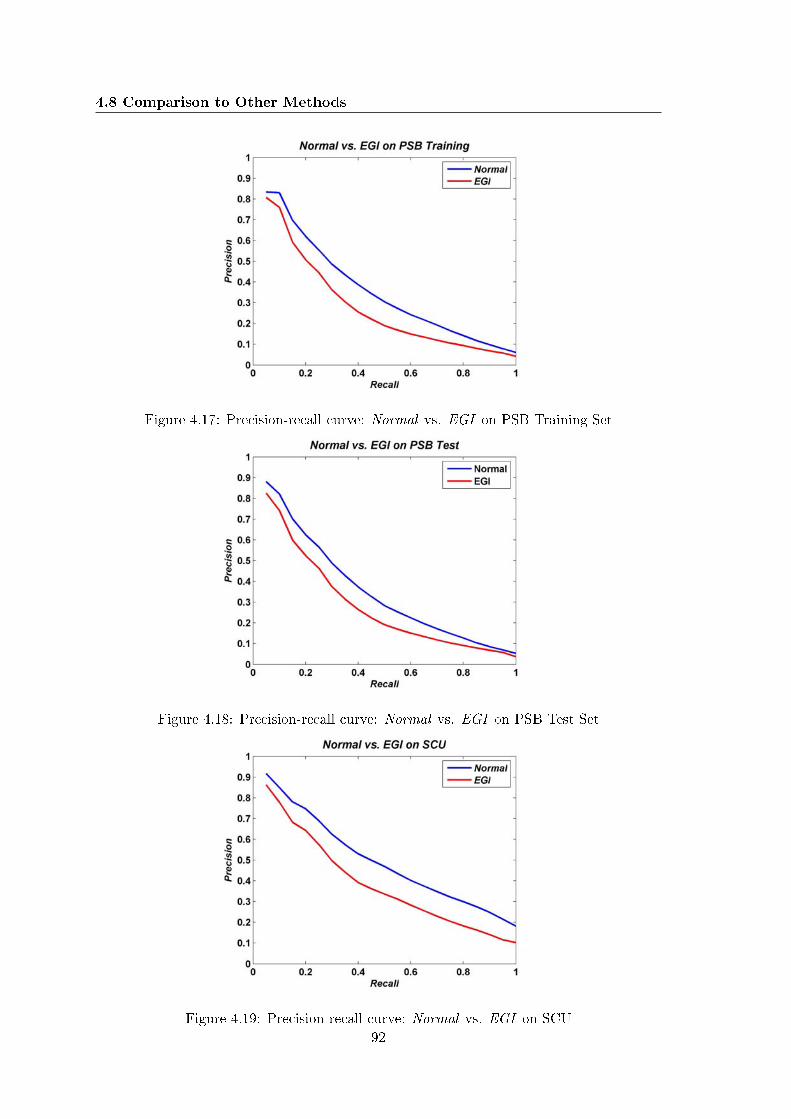
4.8 Comparison to Other Methods
Figure 4.17: Precision-recall curve: Normal vs. EGI on PSB Training Set
Figure 4.18: Precision-recall curve: Normal vs. EGI on PSB Test Set
Figure 4.19: Precision-recall curve: Normal vs. EGI on SCU92

Experiments
Figure 4.20: Precision-recall curve: T-plane vs. 3DHT on PSB Training Set
Figure 4.21: Precision-recall curve: T-plane vs. 3DHT on PSB Test Set
Figure 4.22: Precision-recall curve: T-plane vs. 3DHT on SCU93

4.8 Comparison to Other Methods
Zaharia and Preteux [87] and we have also veried its performance-wise optimality). InFigures 4.20, 4.21 and 4.22, we compare the T-plane and the 3DHT descriptors in terms ofprecision-recall curves. In Table 4.12, we provide the retrieval statistics. On PSB TrainingSet, the T-plane descriptor is better than 3DHT by 1.1% DCG; on PSB Test, by justone tenth DCG percent point. On SCU, on the other hand, the 3DHT has a DCG of72.7% against 72.0% of the T-plane. Since there is no convincing evidence (as comparedto the previous cases) that one method outperforms the other uniformly on the availabledatabases, we can state that the T-plane descriptor and its histogram-based peer 3DHTare performance-wise equivalent.
4.8.2 General Comparison
The results in Sections 4.6 and 4.7 established that our scheme is most eective when weconsider the score fusion of the Radial, T-plane and Sec-Order descriptors. Accordingly,we compare the retrieval performance obtained by the fusion of these descriptors againstother well-known 3D shape descriptors on PSB Test Set. Apart from 3DHT and CAHdescriptors that we have implemented, we have taken the performance scores either fromtheir original works or other comparison studies on PSB Test Set [23, 4].
• Depth-Buer Images (DBI). This descriptor takes its roots from 2D image analysisand describes the object by six depth buer images captured from orthogonal parallelprojections [17, 2]. These binary images are then represented as concatenated vectorsof Fourier coecients of the lowest frequencies. DBI have been the best performingdescriptor on the Konstanz database (cf. Appendix A) [2]. Here, we have taken theperformance scores reported in [4].
• Light Field Descriptor (LFD). Like DBI, LFD is considered as a 2D method as itrepresents an object as a collection of 2D images rendered from the 20 vertices of adodecahedron inscribed in a sphere enclosing the object [50]. The images can thenbe represented as Fourier coecients or 2D Zernike moments as the authors suggest.In order to evaluate the dissimilarity between two objects, the corresponding LFDs,which consist of 20 light eld images each, are aligned over all possible rotations andpairings of vertices, then the minimum distance value is taken. The performancescores reported here are from [23].
• Radialized Extent Function (REXT). This descriptor consists of a collection of spher-ical harmonics-transformed version of shape functions giving the maximal distancefrom the center of mass as a function of spherical coordinates (θ, φ) and radius. SeeSection 1.3.2 and [43, 17] for more details.
• Global Spherical Harmonics Descriptor (GSHD). Similar to REXT, GSHD resultsfrom the decomposition of a sphere into concentric shells of dierent radii [45]. Theintersection of the shape with each of the concentric shells denes a spherical image,which is subsequently transformed to spherical harmonics coecients. GSHD isrendered rotation-invariant by summing the magnitude of the harmonics coecientswithin a given frequency shell [16]. See Section 1.3.2 and [45, 16] for further details.
• Spherical Wavelet Descriptor (SWD). This is a very recently introduced descriptor[46], overcoming the limitations of representing a spherical function in terms of spheri-cal azimuth and elevation angles (θ, φ). The spherical functions are of general type, as
94

Experiments
in REXT and GHSD. Parameterization in terms of (θ, φ) leads to over-accumulationof features near the poles and to sparsity near the equators. Notice that this is thesame type of irregular (or non-uniform) sampling problem that we have dealt within target selection (see Section 2.1.3). In [46], Laga et al. map the spherical domainof the function to a (unfolded) at octahedron, which has regular 2D support. Thissphere-to-octahedron mapping overcomes the irregular sampling problem and trans-forms the function dened on the sphere into an image dened on a regular 2D grid.Afterwards, the descriptor is obtained by applying classical 2D wavelet transformto the 2D image and then collecting a few rst level's transform coecients into avector. Although the term spherical wavelet" is slightly misleading as there is nogenuinely spherical wavelets (e.g., second-generation wavelets [99]) involved in thisprocedure, SWD constitutes the rst instance where the wavelet transform is usedto describe a 3D shape.
• Shape Distributions (D2). This descriptor is simply a histogram of the Euclideandistance between two 3D points on the object's surface [32]. See Section 1.3.1 and[32] for details.
• Generalized Shape Distributions (GSD). This descriptor is introduced as a general-ization to D2 -shape distribution [33]. Accordingly, GSD is a 3D histogram countingthe number of specic local shape pairs at certain distances: two dimensions of thehistogram account for pairs of shape signatures, which are simply k-means quantizedversions of spin images computed on the mesh, while the third dimension records theEuclidean distances of the local shape pairs (at which the signatures are calculated).
• Shape Histograms (SECSHELL). A shape histogram is dened by partitioning the3D space into concentric shells and sectors around the center of mass of a 3D model[34]. The histogram is constructed by accumulating the surface points in the bins (inthe form of shells, sectors, or both) based on a nearest-neighbor rule.
• Voxel Descriptor (VOXEL). This descriptor consists of merely a binary rasterizationof the object boundary into a voxel grid [23].
• 3D Hough Transform Descriptor (3DHT). See Section 1.3.1 and [38, 37] for details.
• Extended Gaussian Image (EGI). See Section 1.3.1 and [35, 36] for details.
• Cord and Angle Histograms (CAH). See Section 1.3.1 and [31] for details.
The specic instances where we compare our framework against the above descriptorsare:
• Radial+T-plane using the Invariant-L1-metric. This instance uses the sum of theinvariant-L1 distance values corresponding to the pdfs of (R, R) and (D, N)-features.Recall that the mentioned invariance is against coordinate axis relabelings and mirrorreections, as described in Section 2.4 and experimented with in Section 4.4.
• Radial+T-plane+Sec-Order using the L1-metric. This instance uses the sum of theplain L1-distance values corresponding to the pdfs of (R, R), (D, N) and (R,A, SI)-features.
95

4.8 Comparison to Other Methods
Table 4.13: Retrieval Statistics (%): State-of-the-Art 3D Shape Descriptors on PSB TestSet
Descriptor NN FT ST DCG NDCG
DBI 66.5 40.3 51.2 66.3 17.1Radial+T-plane (Inv-L1) 68.6 39.3 50.0 65.9 16.4SW 46.9 31.4 39.7 65.4 15.5LFD 65.7 38.0 48.7 64.3 13.6Radial+T-plane+Sec-Order (L1) 65.3 35.2 45.2 62.5 10.4REXT 60.2 32.7 43.2 60.1 6.2GSHD 55.6 30.9 41.1 58.4 3.23DHT 58.8 31.1 39.6 57.7 1.9SECSHELL 54.6 26.7 35 54.5 -3.7VOXEL 54.0 26.7 35.3 54.3 -4.1GSD 43.4 21.5 29.5 49.3 -12.9EGI 37.7 19.7 27.7 47.2 -16.6D2 31.1 15.8 23.5 43.4 -23.3CAH 33.2 15.9 22.9 43.3 -23.5
In Table 4.13, we tabulate the full retrieval statistics corresponding to all of the descrip-tors in decreasing NDCG values. In Figure 4.23, we depict a visual performance landscapein terms of a DCG vs. NN scatter plot. A few comments are in order regarding theseresults:
• The best two descriptors are DBI and Radial+T-plane (Inv-L1). While DCG of ourdescriptor is slightly worse than DBI by 0.4%, its NN score is better by 2.1%.
• The instances of the density-based framework are placed in the top league togetherwith DBI, LFD and SWD.
• DBI and LFD take their roots from 2D ideas as they describe the shape in terms of 2Dprojections of the 3D shape. SWD also employs the wavelet transform in 2D althoughit starts from 3D shape information. Interestingly, except than our descriptors, 2Dmethods perform better than those using directly 3D shape information.
• Figure 4.23 reveals that performance DCG and NN scores are generally correlated,that is, if DCG is high, then NN is also high, and vice versa. The sole exception isSWD whose NN performance is relatively poor as compared to its DCG score.
• Radial+T-plane+Sec-Order marks the performance boundary between 2D methodsand the remaining 3D descriptors.
• The clear performance gap between our descriptors and others such as REXT, GSHDand 3DHT indicates that the density-based framework is currently the most success-ful way to process the 3D shape information for retrieval.
Finally, we note that the density-based framework coupled with FGT is computationallyvery ecient. On a standard laptop PC (1.86 GHz CPU and 1 GB RAM), the Radial,T-plane and Sec-Order descriptors can be computed under one second on average (over 907PSB meshes). Furthermore, even without any dimensionality reduction and compression,
96

Experiments
Figure 4.23: Performance landscape of 3D shape descriptors: DCG vs. NN on PSB TestSet
the storage of these descriptors coded with 16-bit double precision costs only 12 KB onaverage per object.
We close this section by noting that a more impressive retrieval performance on thisdata set has been reported using Funkhouser and Shilane's priority-driven search (PDS )method [4], which belongs to the paradigm of matching by feature correspondences. Givena query object and a database of target objects, all represented by sets of local 3D shapefeatures, the PDS algorithm evaluates how well any subset of query features match targetfeatures. However, as the authors report in [4], this algorithm takes considerably morecomputation time to preprocess the database (4-5 minutes per object), more memoryper object (100 KB per target object), and more time to nd matches than 3D shapedescriptors. In this computationally and memory-wise demanding scheme, there is nounderlying global and compact shape description. DCG of PDS is 75.9%, 10% better thanDBI and Radial+T-plane (Inv-L1), indicating that, performance-wise, there is more wayto go for descriptor-based 3D shape retrieval systems.
4.9 Performance Variation across Databases
In this section, we address the following types of questions concerning the retrieval perfor-mance of the density-based framework over dierent 3D object databases:
• Given a database, which local feature is the most eective?
• Given a feature, which database is the most challenging for the retrieval task?
• In which database, the benets of score fusion become more important?
97

4.9 Performance Variation across Databases
• Does the invariant version of the L1-metric lead to signicant improvements regard-less of the nature of the database?
We illustrate the eectiveness of each feature on each database, as well as the improve-ments due to score fusion and to the use of the invariant metric, using DCG-eye diagrams".These plots will help us make useful inferences at a glance. For instance in Figures 4.24and 4.25, at each (Database, Feature)-pair, we have placed a lled blue circle (hence, thename eye"), whose radius is proportional to the DCG of the feature pdf on that database.We have also put the exact DCG score at the center. The outer circle stands for the idealunit DCG. Clearly, a small white space between the lled circle and the outer one indicatesa good performance.
As in the previous section, we consider the Radial, Tplane and Sec-Order features,whose pdfs summarize respectively zero, rst and second-order local surface information.Figures 4.24 and 4.25 tell us the following:
• For all databases, the T-plane feature performs better than the Radial feature, indi-cating that rst-order surface information is more descriptive than the zero-order.
• The behavior of the Sec-Order feature is interesting: it performs the worst in PSBand the best in SHREC-W, when the L1-distance is used. On a more general basis,the performance of this feature is somewhat correlated with the shape characteristicsof the databases. PSB and SHREC-W represent two extremes in terms of meshregularity and smoothness. SCU and SHREC-W have smooth and manifold mesheswith second-order dierential structure locally present at every mesh point. On theother hand, the meshes in PSB (referred to as triangular soups) are low resolution,non-manifold and cannot always be given a natural orientation; ESB consists ofengineering parts, which contain many joints and at patches. Consequently, formeshes belonging to these two databases, the shape index feature is either not denedeverywhere or unreliable. The curvature estimation being reliable only when there issecond order dierential structure and data is smooth, we observe that the Sec-Orderfeature has unstable performance across dierent databases.
• Figure 4.25, which depicts the results of the Invariant-L1-distance for the Radialand T-plane features, is compatible with Figure 4.24, except that, in SHREC-W,the performance of the Sec-Order -feature is no longer better than the T-plane. Aswe have already demonstrated in Section 4.4 (see Table 4.6), the invariant schemealways improves the performance for all databases and features1.
Regarding the eectiveness of score fusion, we have tested two possible combinations:Radial+T-plane and Radial+T-plane+Sec-Order, using rst the plain L1-metric (Fig-ure 4.26) and then its invariant version (Figure 4.27). Note that, in these gures, thesecombinations are denoted using the initials of the involved features as R+T and R+T +Sto avoid clutter. On the eect of score fusion over dierent databases, we can state thefollowing:
• In any event, the combination of the Radial and T-plane scores improves the resultswith respect to using solely the Radial score or the T-plane score, as established inSection 4.7.
1Observe that the invariant scheme does not apply to Sec-Order as this feature is pose-invariant bydenition.
98

Experiments
Figure 4.24: DCG-eye diagram for Features vs. Databases (L1-metric)
Figure 4.25: DCG-eye diagram for Features vs. Databases (Invariant-L1-metric). Notethat the Invariant-L1-metric improves the average DCG performance over databases by atleast 1.7 points for the T-plane and by 3 points for the Radial features.
99

4.9 Performance Variation across Databases
Figure 4.26: DCG-eye diagram for Score Combinations vs. Databases (L1-metric)
Figure 4.27: DCG-eye diagram for Score Combinations vs. Databases (Invariant-L1-metric)
100

Experiments
Table 4.14: Retrieval Statistics of the Density-Based Framework (%)Database NN FT ST E DCG
PSB 68.6 39.3 50.0 28.6 65.9SCU 80.3 55.9 67.0 37.5 78.3
SHREC-W 94.5 62.7 73.5 53.1 86.7ESB 83.9 45.9 58.6 38.2 75.7
Figure 4.28: Precision-recall curves for the best the density-based descriptors on dierentdatabases
• Adding the Sec-Order score is signicantly eective only for SHREC-W. For otherdatabases, under the plain L1-metric, we obtain a just noticeable improvement byincluding the Sec-Order score. Under the Invariant-L1-metric, it actually worsensthe performance for PSB and does not change anything for ESB. This last fact iscompatible again with our comment above on mesh characteristics.
• Finally, we restate the most eective feature combinations and metrics for a givendatabase below:
PSB: Radial+T-plane scores using Invariant-L1,
SCU: Radial+T-plane+Sec-Order scores using Invariant-L1,
SHREC-W: Radial+T-plane+Sec-Order scores using Invariant-L1,
ESB: Radial+T-plane scores using Invariant-L1.
The full retrieval statistics of these combinations are tabulated in Table 4.14. Thecorresponding precision-recall curves are shown in Figure 4.28. We underline the followingpoints:
101

4.9 Performance Variation across Databases
Figure 4.29: Histograms of class-wise DCGs for dierent databases
Figure 4.30: Distributions of within and between-class distances for dierent databases
102
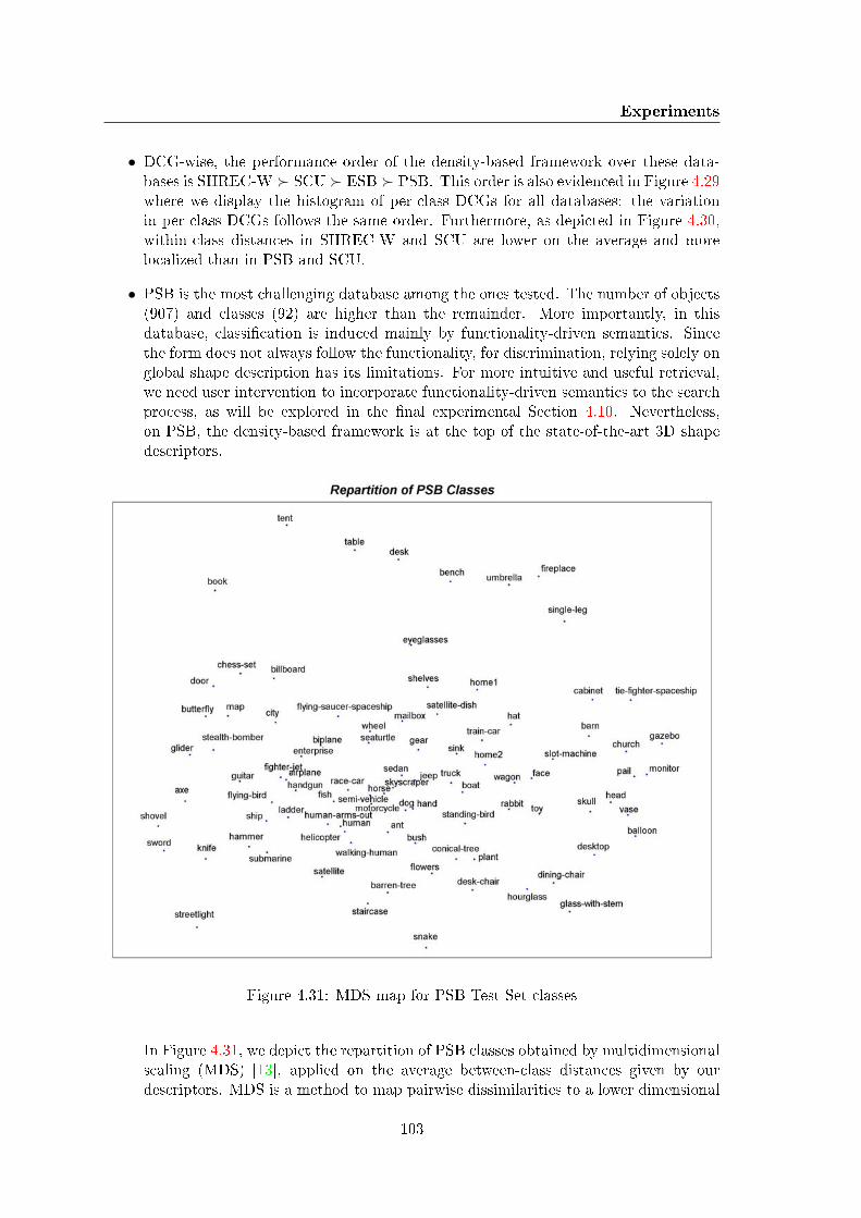
Experiments
• DCG-wise, the performance order of the density-based framework over these data-bases is SHREC-W SCU ESB PSB. This order is also evidenced in Figure 4.29where we display the histogram of per-class DCGs for all databases: the variationin per-class DCGs follows the same order. Furthermore, as depicted in Figure 4.30,within-class distances in SHREC-W and SCU are lower on the average and morelocalized than in PSB and SCU.
• PSB is the most challenging database among the ones tested. The number of objects(907) and classes (92) are higher than the remainder. More importantly, in thisdatabase, classication is induced mainly by functionality-driven semantics. Sincethe form does not always follow the functionality, for discrimination, relying solely onglobal shape description has its limitations. For more intuitive and useful retrieval,we need user intervention to incorporate functionality-driven semantics to the searchprocess, as will be explored in the nal experimental Section 4.10. Nevertheless,on PSB, the density-based framework is at the top of the state-of-the-art 3D shapedescriptors.
Figure 4.31: MDS map for PSB Test Set classes
In Figure 4.31, we depict the repartition of PSB classes obtained by multidimensionalscaling (MDS) [13], applied on the average between-class distances given by ourdescriptors. MDS is a method to map pairwise dissimilarities to a lower dimensional
103

4.10 Statistical Learning-Based Score Fusion
display where the distance order between pairs of entities is preserved as much aspossible. The MDS mapping of PSB classes is open to many interesting observationsshowing that the density-based descriptors capture functionality-driven semantics tosome extent. We itemize below some of the visible regroupments:
In the south-west part of the map, we see a clustering of sharp object classes,such as axe, knife, shovel and sword, used for cutting.
In the north part, we observe a super-class of furniture objects such as table,desk and bench.
In the south part towards the middle, classes such as bush, plant, conical-tree,barren-tree and owers are clustered.
In the middle part towards the west, although within a clutter of irrelevantclasses, we can detect a regroupment of ying objects such as airplane, biplane,ghter-jet, enterprise-spaceship, stealth-bomber and ying-bird.
• We are satised by the performance on SCU (DCG=78.3%), which consists of 513objects in 53 classes. The best DCG performance reported on an earlier release ofthis database, containing 266 objects in 27 classes, was 88% due to the augmentedReeb graph approach [48].
• The least challenging database seems to be SHREC-W. Although it contains a smallnumber of shape classes relative to the remainder, the fact that its classicationis induced by topological equivalences makes it, a priori, a dicult database to bedescribed by geometry-based methods like ours. It is interesting to observe that ageometry-based method performs so well on SHREC-W, especially on the type ofclasses shown in Figure 4.32. We also note that, in the Watertight track of theSHREC'07 event, our shape description scheme outperformed other geometry-basedmethods and had overall the second rank [26].
• The performance on ESB as measured by precision-recall is less impressive thanthe performance reected by the DCG score (75.7%). In fact, the performance forRecall < 0.4 is worse than the more dicult PSB where our method has a DCGof 65.9%. It seems that, on ESB, the density-based framework does not always ndthe correct matches in the very beginning of the list but is eventually capable ofretrieving them, thus lifting the DCG to a satisfactory value.
The main conclusion that we draw from this analysis is that the performance of thedensity-based framework generalizes well for databases with dierent application domains,semantics and shape properties.
4.10 Statistical Learning-Based Score Fusion
In the previous sections, we have investigated the discriminative power of the density-based3D shape description in an unsupervised mode. Now we want to explore the contributionof a certain amount of supervision to the search process. The schemes tested in this sectionwere described in Chapter 3.
In the following two sections, we will quantify the performance of the statistical learning-based score fusion that we interpret as an instance of supervised similarity learning. Weconsider the two applications introduced in Section 3.4, bimodal and two-round searches,
104
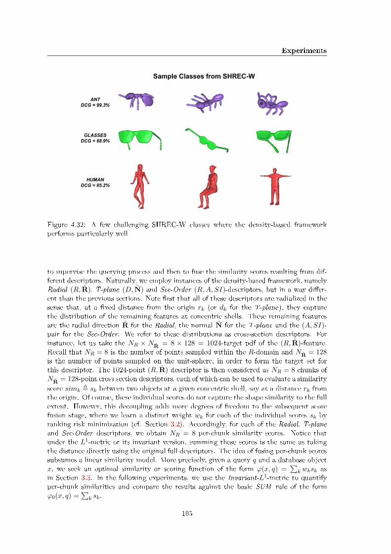
Experiments
Figure 4.32: A few challenging SHREC-W classes where the density-based frameworkperforms particularly well
to supervise the querying process and then to fuse the similarity scores resulting from dif-ferent descriptors. Naturally, we employ instances of the density-based framework, namelyRadial (R, R), T-plane (D, N) and Sec-Order (R,A, SI)-descriptors, but in a way dier-ent than the previous sections. Note rst that all of these descriptors are radialized in thesense that, at a xed distance from the origin rk (or dk for the T-plane), they capturethe distribution of the remaining features at concentric shells. These remaining featuresare the radial direction R for the Radial, the normal N for the T-plane and the (A,SI)-pair for the Sec-Order. We refer to these distributions as cross-section descriptors. Forinstance, let us take the NR × NR = 8 × 128 = 1024-target pdf of the (R, R)-feature.Recall that NR = 8 is the number of points sampled within the R-domain and NR = 128is the number of points sampled on the unit-sphere, in order to form the target set forthis descriptor. The 1024-point (R, R) descriptor is then considered as NR = 8 chunks ofNR = 128-point cross section descriptors, each of which can be used to evaluate a similarityscore simk , sk between two objects at a given concentric shell, say at a distance rk fromthe origin. Of course, these individual scores do not capture the shape similarity to the fullextent. However, this decoupling adds more degrees of freedom to the subsequent scorefusion stage, where we learn a distinct weight wk for each of the individual scores sk byranking risk minimization (cf. Section 3.2). Accordingly, for each of the Radial, T-planeand Sec-Order descriptors, we obtain NR = 8 per-chunk similarity scores. Notice thatunder the L1-metric or its invariant version, summing these scores is the same as takingthe distance directly using the original full descriptors. The idea of fusing per-chunk scoressubsumes a linear similarity model. More precisely, given a query q and a database objectx, we seek an optimal similarity or scoring function of the form ϕ(x, q) =
∑k wksk as
in Section 3.3. In the following experiments, we use the Invariant-L1-metric to quantifyper-chunk similarities and compare the results against the basic SUM rule of the formϕ0(x, q) =
∑k sk.
105

4.10 Statistical Learning-Based Score Fusion
The following performance results have been obtained on a modied version of PSB.Originally, PSB Training and Test Sets do not share the same shape classes. Accordingly,we have merged these two sets into a single one, consisting of 1814 models in 161 classes2.We have then split them into two subsets A and B of sizes 946 and 868, sharing the same161 classes. We will clarify the use of these two sets in the context of the application chosen.This modication lets us treat the problem in an even more challenging complexity thanin the original PSB Test Set, since the number of classes is now increased from 92 to 161.
4.10.1 Performance in the Bimodal Search
Recall that the bimodal search protocol assumes the existence of a training set categorizedinto a xed set of concepts. Learning is done o-line. From the training set, we take oneshape at a time as a query and the remaining ones as database shapes, then feed the pair-wise scores to the algorithm in Section 3.3 to learn a shape-specic SVM. In Section 3.4.1,we had to introduce two dierent heuristics to obtain a weight vector corresponding to eachclass concept, since minimizing directly a per-concept risk functional using all the availableinstances was computationally too complex. We remind that, in the AVE-W heuristic, theweight vector for a given concept class is computed as the average of the per query weightvectors corresponding to the training shapes within that class. In the second PCMIN-Wheuristic, on the other hand, we minimize a per-concept risk by using only support vectorslearned during the prior per-query learning.
In the bimodal experiments, we have taken the PSB Set A as the training set, whichwe have used to learn per-concept weight vectors. PSB Set B has been reserved for testingpurposes. In Table 4.15, we provide the results of fusing 8 Radial -scores and 8 T-planescores, making 16 scores in total. In Table 4.16, we report the performance after including8 more scores corresponding to Sec-Order chunks in addition to Radial and T-plane scores.We also display the results of the basic SUM rule for reference.
Although, the learning-based score fusion does improve the average DCG performancesignicantly on the training set, it does not lead to a signicant gain in the test set (only1% using the AVE-W heuristic). That is, learning-based score fusion does not work wellfor certain concepts. This might be due to heuristics-based learning of per-concept weightvectors, but, we think that the following arguments better explain the situation.
• For some concepts, the linear similarity model might not be exible enough to main-tain good classication accuracy in the score dierence domain. When instancesfrom queries belonging to a certain concept are pooled together, the discriminationproblem in the score dierence domain might become more complex than what canbe solved using a simple linear decision boundary.
• If the linear similarity model were totally unacceptable, we would not expect a goodperformance on the training set either, as in Tables 4.15 and 4.16. In fact, in only4 out of 161 concepts in PSB Set A, the AVE-W fusion of the Radial and T-planescores has worsened the performance by at most 2.3% DCG points with respect tothe baseline SUM rule. In PSB Set B, on the other hand, 61 concepts (again out of161) have suered an average performance loss of 8.5% DCG points.
2The number of classes shared by training and test sets is 21, hence the merged PSB contains 90+92−21 = 161 classes.
106

Experiments
Table 4.15: DCG Performance of Score Fusion on Bimodal Protocol using 8 Radial and 8T-plane-Scores
Rule PSB Set A PSB Set B
SUM 61.9±28.4 61.8±27.9AVE-W 69.4±27.0 62.8±28.1
PCMIN-W 71.1±26.3 62.1±27.6
Table 4.16: DCG Performance of Score Fusion on Bimodal Protocol using 8 Radial, 8T-plane and 8 Sec-Order -Scores
Rule PSB Set A PSB Set B
SUM 61.6±28.1 60.6±28.1AVE-W 71.8±26.5 62.6±28.4
PCMIN-W 74.9±25.2 62.5±27.7
• In Tables 4.17 and 4.18, we provide the DCG scores when we use the basic SUM ruleinstead of learning-based score fusion (AVE-W or PCMIN-W ) for negatively aectedconcepts (i.e., those concepts for which learning-based score fusion has worsened theDCG performance). The right most columns give the number of positively aectedconcepts, indicating in which proportion the learning-based score fusion generalizessatisfactorily. We deduce that the linear similarity model is adequate for the trainingset and generalizes well on the previously unseen instances of ∼100 concepts in thetest set.
• A plausible reason for the lack of generalization for certain concepts is that the scoredierences between training shapes might not be representative enough for thosebetween test shapes. In such cases, the parameters of the linear decision boundarymight overt the training instances.
4.10.2 Performance in the Two-round Search
In the two-round query formulation, the benets of the proposed score fusion schemebecome much more evident. In Section 3.4.2, we have introduced two variants of thisprotocol, with varying amount of user interaction needed. In the on-line variant, thesystem learns a per-query weight vector at query time after having been provided withM marked shapes (either as relevant or not relevant) of the rst round. In the o-linevariant, the user is asked to mark just one single shape among the M displayed ones afterthe rst round. The second round proceeds with the weight vector associated with themarked shape, which has been learned o-line. To evaluate the performance in this searchprotocol, we have reserved the PSB Set A as the database shapes and PSB Set B as thequery shapes. The rst round results have been obtained by the basic SUM rule.
In Figures 4.33 and 4.34, we display the DCG performance of the on-line sub-protocolas a function of the number of marked items M from 4 to 32. Figure 4.33 illustrates theresults for 16 Radial and T-plane scores, while in Figure 4.34, we have also included 8 Sec-Order scores. In these gures, the line at the bottom stands for the DCG of the rst round(i.e., the performance of the SUM rule, DCG = ∼62% for all score combinations). The line
107

4.10 Statistical Learning-Based Score Fusion
Table 4.17: DCG Performance of Score Fusion on Bimodal Protocol using 8 Radial and 8T-plane-Scores when the basic SUM rule instead of learning-based score fusion has beenused for negatively aected concepts
Rule PSB Set B # Positively Aected Concepts
SUM 61.8±27.9 -AVE-W 64.6±24.2 100
PCMIN-W 64.8±23.8 88
Table 4.18: DCG Performance of Score Fusion on Bimodal Protocol using 8 Radial, 8T-plane and 8 Sec-Order -Scores when the basic SUM rule instead of learning-based scorefusion has been used for negatively aected concepts
Rule PSB Set B # Positively Aected Concepts
SUM 61.8±27.9 -AVE-W 64.0±24.1 106
PCMIN-W 64.4±23.9 100
at the top stands for the DCG when all database models are marked as either relevant ornon-relevant, serving as an empirical ideal, i.e., the maximum achievable DCG on this dataset using the presented score fusion algorithm and the running set of description schemes(DCG = ∼75% for Radial and T-plane scores, DCG = ∼79% when Sec-Order scores arealso included). Based on these results, we make the following comments:
• As the number of marked items M increases, we observe a steep increase in the DCGperformance, compatible with theoretical fast rates of convergence proven in [11, 10].
• The DCG prole converges smoothly to the empirical ideal as the user marks moreand more items in the rst round.
• To give certain performance gures, for M = 8, DCG obtained after fusing Radial andT-plane scores becomes ∼67%, giving a 5% improvement compared to the baseline.When the Sec-Order scores are included, the DCG gets ∼68%.
• The 70% DCG barrier is reached after M = 16 marked items for Radial and T-planescores. Adding Sec-Order scores reduces this number down to M = 12, showing infact the Sec-Order scores can indeed be useful in contrast to the case of the basicSUM rule.
In Figures 4.35 and 4.36, we display the DCG performance of the o-line sub-protocolas a function of the number of displayed items M again 4 to 32. We emphasize that, inthis mode, M refers to the number of displayed items and the user interaction needed islimited to mark just one shape, the rst relevant one after the rst round. Accordingly,here, M is not related to the convergence of the algorithm, but just an application-specicparameter determining how far the user is allowed to look for relevant items. IncreasingM does not cost anything in terms of user interaction. After this clarication, we deducethe following:
• At M = 1, combining Radial and T-plane scores boosts the retrieval performance by2.5%, adding the Sec-Order scores by 3.5%.
108

Experiments
• The DCG prole keeps a slow but constant increase as the number of displayed itemsM in the rst round is increased.
• In a typical retrieval scenario, displaying M = 32 items has no cost. These resultstell us that we can obtain DCG improvements by ∼4% with respect to the baseline.Recalling from Section 4.8.2 that the performance of top 3D shape descriptors dieronly by a couple of percentage points, this 4% gain can be considered as signicantand comes virtually at no cost at the querying process. The only bottleneck is theo-line processing of the database shapes to learn the weight vectors, which mayeventually be used in the second round.
When we contrast the on-line and o-line versions of the two-round search protocols, wearrive at a compromise. With on-line score fusion, we can obtain signicant improvementsas the user is asked to mark more and more items. In special applications where theuser voluntarily marks the demanded number of items, the on-line scheme is preferable.The o-line scheme, on the other hand, comes at no cost at query time and still yieldssatisfactory improvements. Sample two-round searches using these two variants are shownin the Appendix E.
109

4.10 Statistical Learning-Based Score Fusion
Figure 4.33: DCG performance of the two-round search with on-line learning as a functionof the number of marked items M in the rst round for Radial and T-plane scores
Figure 4.34: DCG performance of the two-round search with on-line learning as a functionof the number of marked items M in the rst round for Radial, T-plane and Sec-Orderscores
110

Experiments
Figure 4.35: DCG performance of the two-round search with o-line learning as a functionof the number of displayed items M in the rst round for Radial and T-plane scores
Figure 4.36: DCG performance of the two-round search with o-line learning as a functionof the number of displayed items M in the rst round for Radial, T-plane and Sec-Orderscores
111

112

Chapter 5
Conclusion and Perspectives
5.1 Discussion and Conclusion
This thesis has dealt with two fundamentals problems in content-based 3D object retrieval:
(1) How to describe a 3D shape to obtain a reliable representative for the subsequenttask of similarity search?
(2) How to supervise the search process to render it more eective and semantic?
Our contributions concerning the rst problem are as follows:
• We have developed the density-based framework, which produces not only a singlebut a family of shape descriptors at various levels of discrimination.
• Our framework unies histogram-based approaches and enables the passage frommultivariate local surface characterization to global shape description with consider-able ease. Performance-wise, density-based descriptors are signicantly better thantheir histogram-based counterparts1.
• We have shown that the density-based framework proves to be very eective in com-parison to state-of-the-art descriptors. In fact, one of its instances performs betterthan all purely 3D methods and equally well as DBI [2], which is the best 2D methodto date.
• We have tested our framework on four dierent 3D databases, which are selectedfrom distinct domains, in order to show the potential of density-based descriptors ina wide range of applications targeted by the 3D object retrieval research. We haveshown that their performance generalize well on these databases with varying meshquality, semantic content and classication granularity.
• We have developed dedicated dimensionality reduction tools, marginalization andprobability density pruning, which exploit the pdf structure. Furthermore, we haveshown that marginalization can be employed for non-heuristic feature subspace ex-ploration in terms of retrieval performance.
• We have demonstrated that the pdf structure can also be used to guarantee invarianceto certain 3D transformations at matching stage.
1Meanwhile, we note that the T-plane descriptor is just equally well as 3DHT.
113

5.1 Discussion and Conclusion
• We have derived an upper bound on the mean integrated absolute error (MIAE ) ofthe univariate KDE and illustrated the smoothing eect of the bandwidth parame-ter(s) in the context of shape discrimination.
• We have proposed a robust feature calculation scheme in order to obtain more reliablefeature observations from low-resolution meshes.
• Finally, the present work constitutes a rst application of FGT in the 3D domain.This fast approximation scheme turns the KDE method, which is computationallypractical only in a few dimensions, into a computationally very ecient tool for 3Dshape description.
We summarize and discuss the key aspects of the density-based framework below:
• Local Characterization by Joint Features. The features used in the density-based framework are the most basic and direct dierential geometric quantities thatcan be associated with a 3D point lying on a surface. They are intuitive from a shapemodeling perspective and computationally cheap to obtain. Furthermore, the factthat they have mathematically well-dened ranges helps us in the subsequent targetselection.
A joint consideration of these features characterize the surface point completely upto second-order. As we add more dimensions to a multivariate feature, we increaseits specicity. When coupled with the KDE, this family of local features leads to afamily of descriptors, each of which has a dierent level of discrimination.
We have not particularly refrained ourselves from the use of non-invariant features,since invariance at feature-level comes usually at a certain loss of shape information,which cannot be restored back afterwards. We have employed PCA-based normal-ization to discover the major axes of the object to secure rotation invariance withoutloss of information, but at the cost of small errors for which we have relied on therobustness of the KDE. More destructive deciencies such as mislabelings and wrongpolarity assignments have been handled in an exact manner at the matching stage.
• Robust Feature Calculation. Although a triangular mesh leads to a plausiblevisualization of the 3D object at changing levels of resolution, it is somewhat articialand approximates the continuous surface only in the limit, i.e., when the trianglesare suciently small and regular. The Simpson averaging scheme provides a robustfeature calculation option by smoothing the feature values over a mesh triangle sothat mesh irregularities become a lesser problem.
• Global Description via Pdfs. If the pairwise correspondences between two sets offeature observations are known in advance, two shapes can be matched much moreeectively than by using any known 3D shape descriptor. The superior performanceof the PDS method [4] is a manifestation of this fact. This correspondence problemis the main bottleneck for global 3D shape descriptors, which all try to circumventit in one way or another, by registering the shape information on some adequatelychosen grid. The KDE-based framework too eects a kind of registration but, unlikeother approaches, adopts a soft assignment strategy so that a feature observationdoes not only contribute to the closest grid point but also to the nearby ones as afunction of its closeness. This strategy makes the resulting descriptors less sensitiveto small shape variations and extrinsic eects.
114

Conclusion and Perspectives
Closely related to this robustness property is the smoothing behavior of the KDE. Infact, the idea of variability reduction by smoothing has been our main motive in usingKDE. Adapting the example given by Edelman in [100], the method of comparingtwo feature sets must allow for some location uncertainty; otherwise, any small per-turbation would render an object unrecognizable. Testing all possible perturbationswithin a small neighborhood around each feature observation raises combinatorialproblems and hence is unfeasible. One simple way to achieve relative insensitivityto feature location uncertainty is to blur at least one of the feature sets before com-parison, e.g., by convolving it with a bell-shaped kernel such as the Gaussian. Thebandwidth parameter of the kernel accounts for this very uncertainty as discussedin Section 2.2.2. Furthermore, by judiciously adjusting the bandwidth parameter,the descriptors can be rendered smoother or more specic. Large bandwidths en-hance shape commonalities, discard very ne maybe irrelevant details and favor thematching hypothesis by reducing descriptor variation, while small bandwidths pro-duce more faithful descriptors and impose more stringent requirements for a positivematch to occur.
Finally, along with the pragmatic benets mentioned above, describing a 3D shapeby the pdf of its local features is also philosophically appealing. The density-basedframework is a generative method in the sense that it models the conditional densityof a local feature S ∈ RS given a certain shape X. Accordingly, let S be a setof feature observations regarding X. Given two shapes O1 and O2 modeled by theconditional pdfs fS|O1
and fS|O2respectively, we consider the following question:
apart from X, which one of O1 and O2 could have also generated S? If the problemis treated as the one of binary classication, the optimal solution is given by theBayesian decision rule of the form assign S to O1 if fS(S|O1) ≥ fS(S|O2), and toO2 otherwise". The error of this rule can be expressed as [13]
Pr(error) =12
∫RS
min(fS|O1
, fS|O2
),
which can be viewed as a measure of confusion between fS|O1and fS|O2
, as well as ameasure of similarity. In the context of matching via pdfs, to determine which oneof fS|O1
or fS|O2better match fS|X , we have to pick the model O∗, i = 1, 2, which
maximizes the confusion with fS|X , that is,
O∗ = argmaxi=1,2
∫RS
min(fS|X , fS|Oi
).
As shown in Appendix B.1, the above maximization is equivalent to minimizingthe L1-distance between fS|X and fS|Oi
, i = 1, 2. Observe that this equivalence isdistribution-free and independent of feature dimension. This result does not onlyexplain the superior performance of the L1-metric notably against other Minkowskimetrics (cf. Section 4.4), but also provides a rigorous justication for the adequacyof our approach. We conclude that, from the perspective delineated above, thedensity-based framework is the right way to process local surface information forshape matching.
• Marginalization. This fairly general concept of probability theory has found aninteresting application in our framework. Using marginalization, we can switch from
115

5.2 Perspectives
one descriptor to a less specic one, by discarding one or more feature components.Accordingly, we have avoided descriptor computation for every possible feature con-guration and have been able to explore the whole feature space in terms of retrievalperformance very eciently and without resorting to any suboptimal heuristic-basedfeature selection method.
• Invariance at Matching. Another advantage that the pdf structure oers is to se-cure invariance against certain types of object transformations at the matching stage,without the need of recomputing the descriptor for every possible transformation.Starting from the change of variables formula, we have developed a minimization-based similarity measure, completely invariant to coordinate axis relabelings andmirror reections, without sacricing any intrinsic shape information. This measurehas provided signicant performance improvements in all databases.
Concerning the second problem, we have adapted the theoretically well-founded rankingrisk minimization framework [10, 11] to the learning of inter-shape similarities for moreeective and semantic retrieval as shown in Section 4.10 and illustrated in Appendix E.We have cast the problem into one of linearly combining similarity scores, which arisefrom dierent shape descriptors, and have shown that learning can be carried straightfor-wardly by the well-known SVM algorithm. This rigorous score fusion approach allows us tobenet from powerful aspects of individual descriptors by incorporating dierent levels ofsupervision into the search process. Our contributions on similarity learning are as follows:
• To the best of our knowledge, there is no prior work in the 3D domain using statis-tical learning techniques to combine multiple shape descriptors. The present workconstitutes a rst successful attempt to this challenging problem.
• The approach presented in this thesis is a direct application of a recently introducedrigorous statistical framework [10, 11], where consistency and fast rate of convergenceof empirical ranking risk minimizers have been established. These theoretical resultsplace our approach on well-founded grounds.
• Our algorithm operates on scores, and not on descriptors themselves, unlike otherrisk minimization-based approaches [88, 89]. In this sense, it is a general scheme,which does not depend on the type of description and can be used for arbitrary datamodalities as long as one provides similarity scores between entities.
• We have illustrated the use of our scheme in two dierent search protocols. Exper-iments have shown that the two-round protocol benets more from our score fusionframework than the bimodal protocol. The approach is able to boost the retrievalperformance for as many as 100 shape concepts under bimodal query formulations.In the two-round search, on the other hand, we can obtain DCG improvements byas large as ∼10% even with a fairly modest amount of user interaction.
5.2 Perspectives
An immediate research direction to pursue is the extension of invariances, which can beachieved using the scheme presented in Section 2.4, to arbitrary 3D rotations. Such anextension would render the matching completely invariant to rotations as well, and wouldfurther improve the retrieval performance of the density-based descriptors. Apart from 3D
116

Conclusion and Perspectives
object retrieval, recovering the pose of a 3D object with respect to a given reference frameis still an open problem and constitutes the preliminary step in applications such as 3Dmodel reconstruction from existing parts, texture and surface detail mapping, etc. [101].In order to provide a solution to this problem within the density-based framework, we needto nd unit-sphere partitionings that would remain closed under the action of an arbitrary3D rotation as discussed in Section 2.4. Alternatively, we can relax the strict closednessrequirement and rely on nearest-neighbor mapping to establish target correspondencesafter a certain 3D rotation.
Another possible direction of research is towards parametric density estimation. Whilethe KDE approach coupled with FGT proved to be very useful; beyond four dimensions,descriptors get impractically large and the statistical accuracy is no longer guaranteed dueto the curse of dimensionality. In our context, the virtues of parametric mixture modelsare as follows.
• Accuracy problems related to high dimensionality can be more eectively managed.
• They lead to more parsimonious descriptions. If a local feature pdf were available interms of a parameterized analytical form, we would not need to sample it to obtainthe descriptor vector but just store its parameters as the descriptor.
However, we should think of alternative matching schemes since the computational cost ofparametric pdf estimation cannot be aorded at the matching stage. Given a set of i.i.d.feature observations S = skK
k=1 regarding the query and a set of database objects O,each represented by its own parametric pdf, the matching problem would then be to selectthe pdf that best explains the set S by invoking a Bayesian classier of the form assign Sto O∗ such that O∗ = argmax
O∈O
∑k logfS(sk|O)". This maximum likelihood procedure can
be carried eciently since the pdfs are analytically given. Furthermore, using a parametricpdf, we could more conveniently extend the type of invariances that can be secured at thematching stage. The research problems in this direction are:
• Finding a mixture model that would be exible for a wide range of local features,
• Determining the number of parameters involved in the mixture,
• Ecient estimation of the mixture parameters.
Motivated by the fact that our framework is based on pdfs, a natural research directionwould be an information-theoretic analysis of the local surface features. In the presentwork, we have quantied the descriptive power of the local features by their retrievalperformance. Information theory provides us with universal measures for the same endand raises the following interesting issues:
• Let, for instance, Y be the discrete class label of a random 3D object O on whichthe feature S is evaluated. The mutual information value I(S, Y ) stands then forthe amount of information that the feature S contains about the class label Y . It isthe reduction in the uncertainty of the unknown class label due to the knowledge ofthe feature. Consequently, I(S, Y ) arises as a natural measure, which can be usedto order dierent local features in terms of their descriptive power. It would also beinteresting to compare such an ordering, once found, to the one given by an empiricalperformance evaluation.
117

5.2 Perspectives
• If we consider a 3D object as a communication channel, the entropy of the localfeature can be viewed as the average number of bits transmitted to pass its true valueto a recipient. This observation may have implications in 3D mesh compression.
• Along the same line with the above items but on an even more theoretical vein, itis tempting to investigate the relationship between local feature entropy and globalshape complexity.
Finally, the score fusion scheme presented in this thesis leaves the door open for twoimportant research issues:
• Scoring functions can be extended to non-linear forms to cope with situations wherea linear decision boundary is not exible enough to discriminate between score dier-ence vectors. The linear scoring function ϕ(w) = 〈w, s〉 induces a linear discrimina-tion problem in the score dierence domain where the optimization variable is againthe weight vector w. As a consequence, once the weight vector is learned in the scoredierence domain, it can directly be used in the score domain too. In principle, thediscrimination problem can be non-linearized by the kernel trick, in which case thesought-after weight vector no longer lives in the score dierence domain, but in ahigher dimensional space: it is only implicitly given except for some special choicesof the kernel such as the polynomial [94]. In a standard classication problem, thisposes no problem as the decision function can be eciently evaluated in terms ofkernel values. In the retrieval problem as considered in this thesis on the other hand,decision values can only be used to nd the relative rank of an item with respect toanother. The main questions here are:
How can we resolve the nal ordering from relative pairwise ranks in a way fastenough for a real-time application?
Does this resolution phase lead to a consistent nal ordering?
• Although the pairwise ranking risk model has proved to be successful in the scorefusion problem, it has two limitations [20]:
It is not the best metric used in practical retrieval systems.
Only the top few positions of the ranked list are of importance.
The DCG criterion addresses these limitations naturally as rst, by denition, itweights correct results at the top more than those at the bottom and second, itconstitutes the most widely used measure to evaluate the performance of a retrievalalgorithm. Accordingly, one can consider a formulation of the score fusion problemin terms of the DCG criterion.
118

Notations
Density-Based 3D Shape Description
O 3D object (surface)
S Local surface feature
RS Range space of the feature S
skKk=1 Set of observations (sources) for S
RS Discretized version of RS
tnNn=1 Target set (note that RS = tnN
n=1)
fS|O , fS(·|O) Probability density function of S given O
fS(tn|O) Value of the probability density function of S at tn given O
fS|O , [fS(tn|O)]Nn=1 Descriptor vector of the object O w.r.t. S
Statistical Similarity Learning
x, x′ Generic database objects
q Query object
sim(·, ·) Generic similarity function
sk , simk(x, q) kth similarity value between x and q
s , [sk]Kk=1 K-vector of similarities
wk Weight for the kth similarity value
w , [wk]Kk=1 K-vector of weights
ϕ(x, q) , 〈w, s〉 Final similarity (or scoring) function
119

120

Appendix A
3D Object Databases
In this appendix, we list the main features of 3D mesh databases used for research purposes.
• Princeton Shape Benchmark (PSB)
1814 models in 161 classes
Split into two sets: Training (907 models in 90 classes) and Test (907 models in92 classes)
3-level classication hierarchy also available
Example classes: animal, building, furniture, household object, human, musicalinstrument, plant, vehicle
Low resolution, non-regular meshes
Public
http://shape.cs.princeton.edu/benchmark/
• Sculpteur Database (SCU)
858 archaeologically valuable object models: 513 of them categorized in 53classes
2-level classication hierarchy also available
Example classes: amphora, vase, pavement, statue, relievo, mould
High resolution, watertight meshes
Private
http://www.sculpteurweb.org/
http://www.tsi.enst.fr/3dmodels/
• SHREC Watertight Database
400 models in 20 classes
Example classes: ant, chair, glasses, hand, human, octopus, spring
Topology-driven equivalence classes
High resolution, watertight meshes
Open to SHREC'07 participants
121

http://watertight.ge.imati.cnr.it/
• Purdue Engineering Shape Benchmark (ESB)
865 CAD models in 45 classes
2-level classication hierarchy also available
Example classes: bearing, contact switch, elbow, gear, handle, housing, thinplate, T-shaped part, U-shaped part
Middle resolution, watertight meshes
Open to SHREC'07 participants
https://engineering.purdue.edu/PRECISE/shrec/
http://shapelab.ecn.purdue.edu/Benchmark.aspx
• Konstanz Database
1839 models: 473 classied
Public
http://merkur01.inf.uni-konstanz.de/CCCC/
• MPEG-7 Database
227 models: all classied
Private
http://merkur01.inf.uni-konstanz.de/CCCC/
• National Taiwan University Database (NTU)
10911 models
Public
http://3d.csie.ntu.edu.tw/ dynamic/database/index.html
• Informatics-Telematics Institute Database (ITI)
544 models in 13 classes
Example classes: animal, airplane, helicopter, car, couch, human
Public
http://3d-search.iti.gr/3DSearch/index.html
http://shrec.iti.gr/download.html
• McGill Database
Articulated object models
Public
http://www.cim.mcgill.ca/ shape/benchMark/
• Carnegie Mellon Database
∼2000 models
122

3D Object Databases
Private
http://amp.ece.cmu.edu/projects/3DModelRetrieval/
• SHREC 3D Face Database
1000 3D face models
Open to SHREC'07 participants
http://give-lab.cs.uu.nl/SHREC/shrec2007/
123

124

Appendix B
Standard Dissimilarity Measures
In this appendix, we provide denitions for some of the standard measures to evaluate the
dissimilarity between two histogram-based descriptors f = [fi]Ni=1 and f ′ =
[f ′j
]N ′
j=1. Except
for the earth mover's distance, we assume that descriptors have the same dimension, i.e.,N = N ′, their entries fi and f ′j are real numbers and they sum to one, i.e.,
∑i fi =
∑j f ′j =
1. In the following denitions, the index i runs from 1 to N and j from 1 to N ′.
B.1 Lp-Distances
For p ≥ 1, these measures are also known as Minkowski distances, L1, L2 and L∞ beingthe most commonly used ones, especially because they are computationally very cheap.For p < 1, Lp-measures are called as sublinear norms. They emphasize small point-wise absolute dierences |fi − f ′i | more than Minkowski norms. On a general basis, as pdecreases, small dierences, typically in the tails of distributions become more and moreimportant. Lp-distances for vectors are given by
Lp(f , f ′) =
(∑i
∣∣fi − f ′i∣∣p)(1/p)
.
L1-distance, in particular, has an interesting connection with binary classication [7]. Sup-pose that an observation s (regarding a random variable S ∈ RS) comes from one of thetwo equally likely classes C and C′ represented by densities f and f ′ respectively. Themisclassication probability Pr(error) of a Bayesian decision rule of the form: assign s toC if f(s) ≥ f ′(s), and to C′ otherwise, is given by
Pr(error) =12
∫RS
min(f, f ′).
Using the identity min(a, b) = |a+b|2 − |a−b|
2 , it can be shown that
Pr(error) =12− 1
4
∫RS
|f − f ′|,
=12− 1
4L1(f, f ′).
Thus, the maximum Bayesian probability of misclassication occurs at the minimum L1-distance between class-conditional densities f and f ′.
125

B.2 Symmetric Kullback-Leibler Distance
B.2 Symmetric Kullback-Leibler Distance
In probability theory, the Kullback-Leibler divergence KLdiv is a non-symmetric measureof dierence between two probability distributions. A symmetric version of this measurecan be obtained as follows
KL(f , f ′) = KLdiv(f ||f ′) + KLdiv(f ′||f),
=∑
i
filogfi
f ′i+∑
i
f ′i logf ′ifi
,
=∑
i
(fi − f ′i)logfi
f ′i.
Note that KLdiv is a special case of the more general α-divergence given by (in the con-tinuous case)
αdiv(f ||f ′) =1
α− 1log
∫f ′(
f
f ′
)α
,
where α ∈ [0, 1]. KLdiv can be obtained in the limit as α → 1.
B.3 χ2-Divergence
In statistics, χ2-test is a generic method to decide whether two data sets are drawn from thesame distribution or not. The acceptance hypothesis is retained based on the signicanceof the χ2-divergence value given below
χ2(f , f ′) =∑
i
(fi − f ′i)2
fi + f ′i.
In matching two descriptors, the above value is taken directly as a measure of dissimilaritywithout performing any signicance test.
B.4 Bhattacharyya Distance
Bhattacharyya Distance is an alternative measure that can be used to decide whether twostatistical distributions dier or not:.
B(f , f ′) = 1−∑
i
√fif ′i .
In view of the discussion for the L1-distance, Bhattacharyya distance can be related to theBayesian probability of misclassication. Consider the binary classication setup as in theabove. Accordingly, from (B.1) and the fact that min(a, b) ≤
√ab, we have
Pr(error) ≤∫RS
√ff ′.
Thus, an upper bound on the Bayesian probability of misclassication is maximized at theminimum Bhattacharyya distance between class-conditional densities f and f ′.
126

Standard Dissimilarity Measures
B.5 Histogram Intersection
Histogram intersection is originally proposed for matching color histograms [67]. Theassociated distance function is expressed as
HI(f , f ′) = 1−∑
i
min(fi, f′i).
By invoking min(a, b) = |a+b|2 − |a−b|
2 , we can see that HI is equivalent to L1-distance.
B.6 Earth Mover's Distance
A descriptor entry fi can be a two-tuple (mi, wi), where mi ∈ Rm is interpreted as a bincenter in a multidimensional histogram and wi ∈ R as the amount of mass concentrated
around mi. In such a case, descriptors f = [(mi, wi)]Ni=1 and f ′ =
[(m′
j , w′j)]N ′
j=1are called
as signatures. Let W be the total amount of mass contained in the descriptor f , that is,W =
∑i wi (likewise for W ′), and let η be a ground distance between bin centers such as
L2. The earth mover's distance is then dened as the minimum value of an optimizationproblem [102]:
EMD(f , f ′) = mincij
∑i,j η(mi,m
′j)cij
min (W,W ′),
such that
cij ≥ 0,∀i, j,∑j
cij ≤ wi,∀i,∑i
cij ≤ w′j ,∀j,∑
i,j
cij = min(W,W ′) ,
where the optimization variables cij stand for the amount of mass to be carried from thebin mi to the bin m′
j . The use of EMD is motivated by the fact that the bin centers intwo dierent descriptors might not be aligned. The computational complexity of the aboveprogram is above O(N3) and limits its practical usability for large signatures. A recentlyintroduced algorithm reduces this complexity down to an empirically shown O(N2) whenthe ground distance η is chosen as L1 [103].
127

128

Appendix C
KDE and Related Issues
In this appendix, we provide some derivations related to kernel density estimation (KDE).First, in C.1, we derive the univariate KDE using a xed scalar bandwidth as in [13].In C.2, we derive the upper bound on the mean integrated absolute error (MIAE ) inthe univariate shape description context, which were used to illustrate the smoothingeect of the KDE in Section 2.2.1. This derivation is our original contribution. In C.3,following [7], we recapitulate the asymptotic mean integrated squared error (AMISE ) andextend the expression for the univariate Scott bandwidth to the case of arbitrarily weightedobservations.
C.1 Derivation
Suppose we want to estimate the pdf fS of some random variate S ∈ Rm at some targett ∈ Rm. Let N (t) be some neighborhood around the target t, with volume V ol[N(t)]. Theprobability that S falls inside N (t) is
PrS ∈ Nt =∫N (t)
fS(u)du.
For suciently small N (t) and continuous fS , a reasonable approximation to fS(t) wouldthen be
fS(t) ' PrS ∈ N (t)V ol[N (t)]
. (C.1)
Given a set of independent observations skKk=1, a natural estimate for PrS ∈ Nt can
be obtained by counting the number of sk's falling inside N (t) in which case we can write
PrS ∈ Nt '#sk's inside N (t)
K=
1K
K∑k=1
Isk ∈ N (t), (C.2)
where I· is one when the predicate inside the curly brackets is true, and zero otherwise.Now suppose momentarily that the neighborhood N (t) is an m-dimensional hypercubewith edge length h so that V ol[N(t)] = hm. Accordingly, combining Eqs. C.1 and C.2, wecan write
fS(t) ' 1Khm
K∑k=1
Isk ∈ N (t). (C.3)
129

C.2 Derivation of the Upper Bound on MIAE
The kernel family of density estimators arises in a quest to generalize Eq. C.3. Observethat, when the neighborhood is chosen to be a hypercube, we can analytically express the0-1 counting function I· as
Isk ∈ N (t) = K(I(t− sk)
h
),
where K is interpreted as a kernel function and I is the m×m identity matrix. Thus, the0-1 counting function occurs as just a special case of a generic kernel K, corresponding toa hypercube neighborhood of xed volume. One can also identify h−1I as the bandwidthparameter matrix H, which remains the same for all the observations, i.e., Hk = H,∀k.
Allowing kernels that are smoother than the 0-1 counting function lies at the heart ofKDE methodology. The specic form of the kernel paramaterized by the bandwidth Hdetermines implicitly the shape and the size of the neighborhood chosen. In fact, one doesnot need to dene a crisp neighborhood such as a hypercube. When a smooth function ofthe observation-target distance is chosen as a kernel, all the observations contribute to thedensity estimate. In a nutshell, closer observations contribute more, far-away ones less. Asa result, KDE can also be viewed as a data interpolation method. Thus, the KDE equationfor arbitrary kernels reads as
fS(t) =1
K |H|
K∑k=1
K(H−1
k (t− sk)). (C.4)
For the Gaussian kernel given by
KGaussian(u) = (2π)−m/2exp(− 1
2‖u‖2
),
we have
fS(t) =1
(2π)−m/2K |H|
K∑k=1
exp(− 1
2(t− sk)T H−2(t− sk)
). (C.5)
Eqs. 2.4 and 2.5 in Section 2.2 are more general forms of Eqs. C.4 and C.5, where eachobservation induces a dierently sized of neighborhood around the target t through thevariable bandwidth parameter Hk. Another distinction is the scalar importance weight wk
associated with each observation, which is set to 1/K above, in the abscense of any priorinformation regarding the sampling density.
C.2 Derivation of the Upper Bound on MIAE
Let f and f ′ be two real-valued functions with scalar domains, given by
f(t) =1√
2πhK
K∑k=1
exp
−1
2
(t− sk
h
)2
,
f ′(t) =1√
2πhK
K∑k=1
exp
−1
2
(t− s′k
h
)2
,
where sk's are known deterministic scalars, s′k's are their randomly perturbed versions sothat s′k = sk + εk. The additive perturbations εk's are zero-mean i.i.d. random variables.
130

KDE and Related Issues
Both f and f ′ are positive and integrate to one. In the following, we derive an upperbound on the expected variation between f and f ′ in the integrated absolute sense. Wecall this measure of variation as mean integrated absolute error (MIAE ). Concretely,
MIAE(f, f ′) , E
∫R
∣∣f − f ′∣∣ ,
=∫
RE∣∣f − f ′
∣∣,where E· is the expectation operator. We can write the point-wise dierence f(t)−f ′(t)as
f(t)− f ′(t) =1√
2πhK
K∑k=1
exp
−1
2
(t− sk
h
)2[
1− exp
(t− sk)εk
h2− 1
2
(εk
h
)2]
.
Let us now use the Hermite identity exp(2ab − b2) =∑∞
n=01n!b
nHn(a), where Hn are theHermite polynomials. Identifying that a = (t− sk)/
√2h and b = εk/
√2h, we get
f(t)− f ′(t) =1√
2πhK
K∑k=1
∞∑n=1
exp
−1
2
(t− sk
h
)2
1n!
(εk√2h
)n
Hn
(t− sk√
2h
).
Taking the expected absolute value of the above expression and using the triangle inequal-ity, we obtain
E∣∣f(t)− f ′(t)
∣∣ ≤ 1√2πhK
∞∑n=1
12n/2n!
E |ε|n
hn
K∑k=1
exp
−1
2
(t− sk
h
)2∣∣∣∣Hn
(t− sk√
2h
)∣∣∣∣ ,where we have used the fact that E |εk| = E |ε| ,∀k by the i.i.d. assumption. Now, inte-grating both sides of the above expression with respect to t, we obtain an upper bound onMIAE,
MIAE(f, f ′) ≤∞∑
n=1
Cn(h)2n/2n!
E |ε|n
hn, (C.6)
where Cn(h) , 1√2πh
∫e−u2/2h2 |Hn( u√
2h)|du. Furthermore, Cramer's inequality for Her-
mite polynomials tells that |Hn(u)| ≤ C2n/2√
n! eu2/2, where C is a numerical constantless than 1.09 in value [8]. Thus,
Cn(h) ≤(C2n/2
√n!) 1√
2πh
∫exp
(− u2
2h2
)exp
(u2
4h2
)du,
=(C2n/2
√n!) √
2√2π√
2h
∫exp
(−1
2u2
2h2
)du,
= C2(n+1)/2√
n! .
Finally, combining the above result with the bound in (C.6), we get
MIAE(f, f ′) ≤ C
∞∑n=1
1√n!
E |ε|n
hn, (C.7)
where we have lumped the√
2 factor into the constant C.
131

C.3 AMISE and the Scott Bandwidth
C.3 AMISE and the Scott Bandwidth
The asymptotic mean integrated squared error (AMISE ) of a univariate kernel estimatoris given by the sum of the asymptotic integrated squared bias (AISB) and the asymptoticintegrated variance (AIV ):
AMISE(h) = AISB(h) + AIV (h).
When the observations are equally weighted by 1/K, we have [7]:
AISB(h) =14‖µ2(K)‖2 R(f ′′)h4,
AIV (h) =R(K)Kh
,
where R(φ) ,∫
φ2 and ‖µ2(K)‖ ,∫
u2K(u)du. Observe that AISB does not dependon the number of observations K neither on how they are weighted. Thus, to derive anexpression for the AMISE -optimal bandwidth for arbitrarily weighted observations by wk,where
∑k wk = 1, we need to work with the variance term as follows. The univariate
kernel estimator f of a density f is given by
f(s) =1h
K∑k=1
wkKh (s, sk),
where Kh(s, sk) , 1hK(
s−skh
)and skK
k=1 are i.i.d. realizations of a random variable S.The variance of the estimate f(s) is given by
V ar
f(s)
= W V ar Kh(s, S) ,
= W E Kh(s, S)2 −W [E Kh(s, S)]2 ,
where W ,∑K
k=1 w2k. Expanding the rst and the second terms above in Taylor series
and then integrating the result, the integrated variance IV can be shown to be [7]:
IV (h) = WR(K)
h−W R(f) + . . . .
Finally, based on Theorem 6.1, page 131 in [7], we get
AMISEw(h) = WR(K)
h+
14‖µ2(K)‖2 R(f ′′)h4,
h∗ =[W
R(K)‖µ2(K)‖2 R(f ′′)
]1/5
,
for the univariate kernel estimator using arbitrarily weighted observations.To nd the Normal reference rule or the Scott bandwidth, we proceed by assuming a
Gaussian reference density f with variance σ2 and a Gaussian kernel K. Plugging in thecorresponding expressions for R(f ′′), R(K), and ‖µ2(K)‖2, we obtain the Scott bandwidth:
hScott =(
43W
)1/5
σ.
132

KDE and Related Issues
The m-dimensional multivariate generalization of this result for a diagonal bandwidthmatrix H = diag(h1, . . . , hm) can be obtained by working with multidimensional Taylorexpansions [7]. Here, we simply state the result:
HScott =(
4m + 2
W
)1/(m+4)
diag(σ1, . . . , σm).
133

134

Appendix D
Marginalization Results
Starting from the pdf of an m-dimensional feature S = (S1, . . . , Sm), the marginalizationanalysis is carried in m−1 stages. At a certain stage t = 1, . . . ,m−1, we integrate t-tupleof components out from the pdf of the original m-dimensional feature. At a given stage t,there are
(mt
)such operations, yielding 2m − 2 possible marginalizations in total.
The following tables present the DCG results of the exhaustive marginalization analysisapplied on the pdf-based descriptor of the 6-dimensional feature (R, Rx, Ry, Nx, Ny, A),as presented in Section 4.6.2. The analysis involves 5 stages, thus the total number ofmarginalizations is 2m − 2 = 62. In these tables, a given row corresponds to a specicmarginalization where the retained components are indicated by gray-shaded cells and theremoved one(s) by white cell(s). The black cell at the right-most column stands for thefeature conguration, which yields the maximum DCG of the corresponding stage.
135
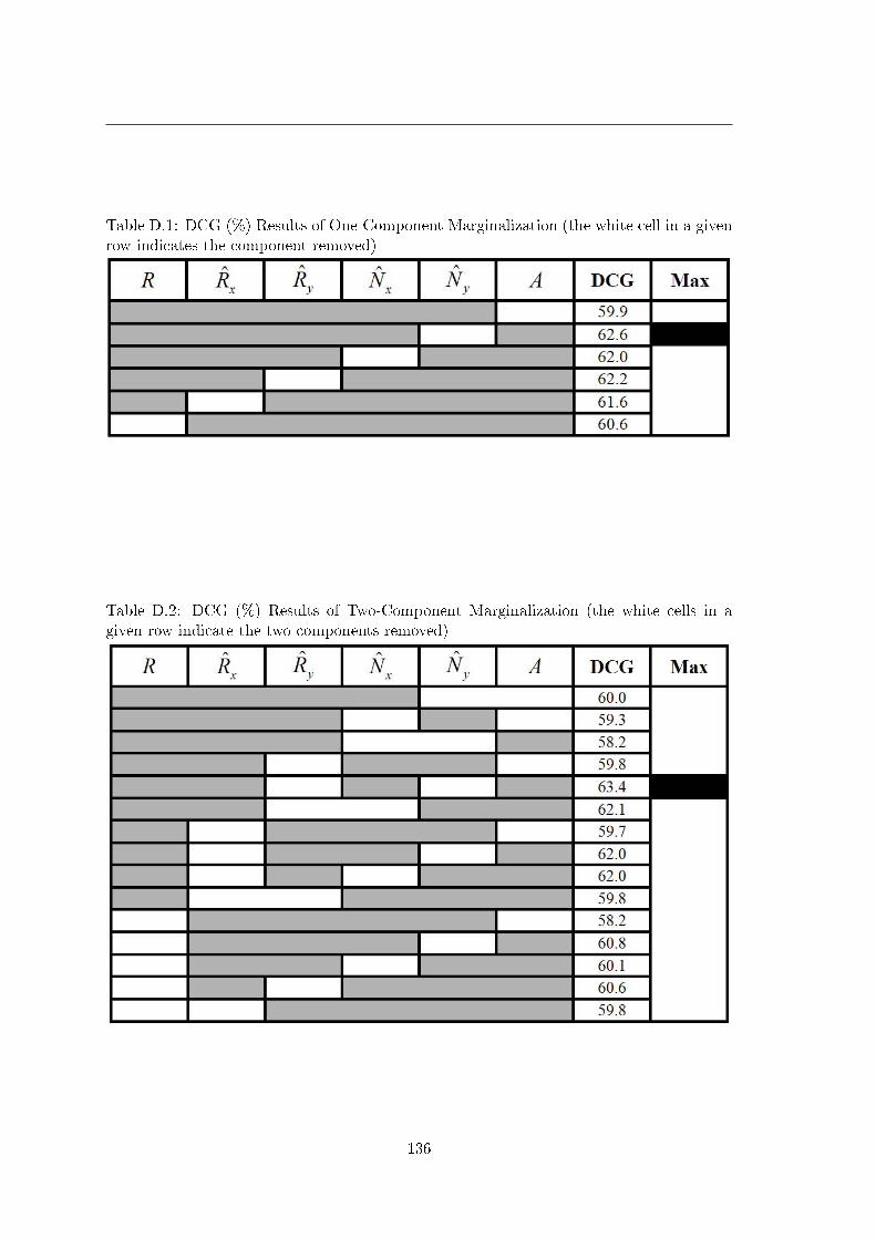
Table D.1: DCG (%) Results of One-Component Marginalization (the white cell in a givenrow indicates the component removed)
Table D.2: DCG (%) Results of Two-Component Marginalization (the white cells in agiven row indicate the two components removed)
136

Marginalization Results
Table D.3: DCG (%) Results of Three-Component Marginalization (the white cells in agiven row indicate the three components removed)
137

Table D.4: DCG (%) Results of Four-Component Marginalization (the white cells in agiven row indicate the four components removed)
Table D.5: DCG (%) Results of Five-Component Marginalization (the white cells in agiven row indicate the ve components removed)
138

Appendix E
Sample Two-round Searches
In this appendix, we illustrate the two-round application of learning-based score fusion.We remind the on-line and o-line versions of this protocol below:
• On-line.
The user enters a query shape.
In the rst round, the system returns M ranked databases shapes using thebasic SUM rule and asks the user to label all of them as either relevant ornon-relevant.
The system learns a weight vector using the score dierence vectors correspond-ing to these marked shapes on-line.
In the second round, the system uses the learned weight vector to evaluate aweighted similarity score and returns a new set of database shapes.
• O-line.
The user enters a query shape.
In the rst round, the system returns M ranked databases shapes using thebasic SUM rule and asks the user to label just one shape, the very rst one thathe/she nds relevant.
In the second round, the system uses the weight vector corresponding to themarked shape, which has already been learned o-line, to evaluate a weightedsimilarity score and returns a new set of database shapes.
Figures E.1 and E.2 illustrate two applications of the on-line mode using a couch" and ahuman" 3D model as queries respectively. Figures E.3 and E.4 illustrate two applicationsof the o-line mode using a plant" and a bench" 3D model as queries respectively.
139

Figure E.1: Two-round search with on-line learning on a couch" query. In the rst round,only the rst-ranked item is relevant (marked as green, the remainder as red); the secoundround retrieves four more couch" models. Notice also that the fourth-ranked bench"model is plausible to human intuition but not used as a positive result in performanceevaluation.
140

Sample Two-round Searches
Figure E.2: Two-round search with on-line learning on a human" query. In the rst round,the system returns non-relevant car", bird" and helicopter" models (marked as red) inaddition to other human" models (marked as green); the secound round eliminates thenon-relevant ones and returns only human" models.
141

Figure E.3: Two-round search with o-line learning on a plant" query. In the rst round,the very-rst relevant item occurs only at the fourth position (marked as green); the secondround retrieves two more crisply correct matches along with three tree" models (positions:3, 6 and 8) and one potted-plant", which are also plausible (but not used as positive resultsfor performance evaluation). The only totally non-relevant item of the second round is theseventh-ranked human" model.
142

Sample Two-round Searches
Figure E.4: Two-round search with o-line learning on a bench" query. In the rst round,the rst item is marked as relevant (in green); the second round returns four more bench"models at positions 2, 3 and 7 respectively. The eight-ranked desk" is semantically similarto the query as well.
143

144

Appendix F
Publications
F.1 Publications Related to the Thesis
1. C. B. Akgül, B. Sankur, Y. Yemez, F. Schmitt. Density-Based 3D Shape Descrip-tors. EURASIP Journal on Advances in Signal Processing, vol. 2007, Article ID32503, 2007.
2. C. B. Akgül, B. Sankur, F. Schmitt, Y. Yemez. Multivariate Density-Based 3DShape Descriptors. Proceedings of the Shape Modeling International 2007 (SMI'07),Lyon, France, June 13-15, 2007.
3. C. B. Akgül, F. Schmitt, B. Sankur, Y. Yemez. Multivariate Density-Based 3DShape Descriptors. Proceedings of the Shape Retrieval Context 2007 (SHREC'07),Lyon, France, June 15, 2007.
4. C. B. Akgül, B. Sankur, Y. Yemez, F. Schmitt. Improving Eciency of Density-Based Shape Descriptors for 3D Object Retrieval. Computer Vision / ComputerGraphics Collaboration Techniques (MIRAGE07), Springer LNCS Series, vol. 4418,pp. 330-340, INRIA Rocquencourt, France, March 28-30, 2007.
5. C. B. Akgül, B. Sankur, F. Schmitt, Y. Yemez. Density-based Shape Descriptorsfor 3D Object Retrieval. International Workshop on Multimedia Content Represen-tation, Classication and Security (MRCS'06), Springer LNCS Series, vol. 4105, pp.322-329, Istanbul, Turkey, September 11-13, 2006.
6. C. B. Akgül, B. Sankur, Y. Yemez, F. Schmitt. A Framework for Histogram-Induced 3D Descriptors. Proceedings of the 14th European Signal Processing Confer-ence (EUSIPCO'06), Florence, Italy, September 4-8, 2006.
7. C. B. Akgül, B. Sankur, F. Schmitt, Y. Yemez. Feature-Level and Descriptor-Level Information Fusion for Density-Based 3D Shape Descriptors. IEEE 15th SignalProcessing and Communications Applications (SIU), Eskisehir, Turkey, June 2007.
8. C. B. Akgül, B. Sankur, F. Schmitt, Y. Yemez. A New Framework for 3D ShapeDescriptors. IEEE 14th Signal Processing and Communications Applications (SIU),Antalya, Turkey, April 2006.
145

F.2 Other Publications in 2004-2007
9. C. B. Akgül, B. Sankur, F. Schmitt, Y. Yemez. 3D Object Matching via Mul-tivariate Shape Distributions. IEEE 13th Signal Processing and CommunicationsApplications (SIU), Kayseri, Turkey, May 2005.
In Preparation
1. Score Fusion by Ranking Risk Minimization for 3D Object Retrieval, 2007.
2. 3D Pose Normalization using Density-Based Shape Descriptors, 2007.
F.2 Other Publications in 2004-2007
1. C. B. Akgül, B. Sankur, A. Akin. Extraction of cognitive activity related wave-forms from functional near infrared spectroscopy signals. Medical and BiologicalEngineering and Computing, vol. 44, pp. 945-958, November 2006.
2. C. B. Akgül, B. Sankur, A. Akin. Spectral analysis of event-related hemodynamicresponses in functional near infrared spectroscopy. Journal of Computational Neu-roscience, vol. 18, pp. 67-83, January 2005.
3. C. B. Akgül, B. Sankur, A. Akin. Extraction of cognitive activity related wave-forms from functional near infrared signals. Proceedings of the 14th European SignalProcessing Conference (EUSIPCO'06), Florence, Italy, September 4-8, 2006.
4. C. B. Akgül, B. Sankur, A. Akin. Evidence of cognitive activity in functionalnear infrared spectroscopy signal. OSA Optical Techniques in Neuroscience TopicalMeeting, Miami Beach, Florida, USA, April 2004.
5. D. Lesage, J. Darbon, C. B. Akgül. An Ecient Algorithm for Connected At-tribute Thinnings and Thickenings. International Symposium on Visual Computing(ISVC'06), Springer LNCS Series, vol. 4292, pp. 393-404, Lake Tahoe, Nevada,USA, November 6-8, 2006.
6. J. Darbon, C. B. Akgül. An Ecient Algorithm for Attribute Openings and Clos-ings. Proceedings of the 13th European Signal Processing Conference (EUSIPCO'05),Antalya, Turkey, September 2005.
7. C. B. Akgül, B. Sankur, A. Akin. Evidence of cognitive activity in functional op-tical signals. IEEE 12th Signal Processing and Communications Applications (SIU),Cesme, Turkey, April 2004.
8. C. B. Akgül, B. Sankur, A. Akin. Extraction of cognitive activity related waveformsfrom functional optical signals. IEEE 12th Signal Processing and CommunicationsApplications (SIU), Cesme, Turkey, April 2004.
9. E. Yörük, C. B. Akgül. Color image segmentation using fast watersheds and PDE-based regularization. IEEE 12th Signal Processing and Communications Applications(SIU), Cesme, Turkey, April 2004.
146

Bibliography
[1] S. Ortiz. 3D searching starts to take shape. Computer, 37(8):2426, 2004.
[2] B. Bustos, D. A. Keim, D. Saupe, T. Schreck, and D. V. Vranic. Feature-basedsimilarity search in 3D object databases. ACM Comput. Surv., 37(4):345387, 2005.
[3] J. W. H. Tangelder and R. C. Veltkamp. A survey of content based 3D shape retrievalmethods. In Proc. of the Shape Modeling International 2004 (SMI'04), pages 145156, Genoa, Italy, 2004.
[4] T. Funkhouser and P. Shilane. Partial matching of 3D shapes with priority-drivensearch. In Symposium on Geometry Processing, June 2006.
[5] N. Iyer, S. Jayanti, K. Lou, Y. Kalyanaraman, and K. Ramani. Three-dimensionalshape searching: state-of-the-art review and future trends. Computer-Aided Design,37(5):509530, April 2005.
[6] W. Härdle, M. Müller, S. Sperlich, and A. Werwatz. Nonparametric and Semipara-metric Models. Springer Series in Statistics. Springer, 2004.
[7] D. W. Scott. Multivariate Density Estimation. Theory, Practice and Visualization.Wiley, New York, 1992.
[8] L. Greengard and J. Strain. The fast Gauss transform. SIAM J. Sci. Statist. Comput.,12:7994, 1991.
[9] C. Yang, R. Duraiswami, N. A. Gumerov, and L. Davis. Improved fast Gauss trans-form and ecient kernel density estimation. ICCV, 1:464, 2003.
[10] S. Clémençon, G. Lugosi, and N. Vayatis. Ranking and scoring using empirical riskminimization. In COLT, pages 115, 2005.
[11] S. Clémençon, G. Lugosi, and N. Vayatis. Ranking and empirical risk minimizationof U-statistics. The Annals of Statistics, to appear, 2007.
[12] R. J. Campbell and P. J. Flynn. A survey of free-form object representation andrecognition techniques. Comput. Vis. Image Underst., 81(2):166210, 2001.
[13] R. O. Duda, P. E. Hart, and D. G. Stork. Pattern Classication. Wiley-Interscience,2000.
[14] T. Hastie, R. Tibshirani, and J. Friedman. The Elements of Statistical Learning:Data Mining, Inference, and Prediction. Springer-Verlag, New York, NY, 2001.
147

BIBLIOGRAPHY
[15] D. G. Kendall. The diusion of shape. Adv. Appl. Probab., 9:428430, 1977.
[16] M. Kazhdan, T. Funkhouser, and S. Rusinkiewicz. Rotation invariant spherical har-monic representation of 3D shape descriptors. In Proceedings of the 2003 Eurograph-ics/ACM SIGGRAPH symposium on Geometry Processing (SGP'03), pages 156164,Aire-la-Ville, Switzerland, 2003. Eurographics Association.
[17] D. V. Vrani¢. 3D Model Retrieval. PhD thesis, University of Leipzig, 2004.
[18] E. Paquet, A. Murching, T. Naveen, A. Tabatabai, and M. Rioux. Description ofshape information for 2D and 3D objects. Signal Processing: Image Communication,16:103122, 2000.
[19] J. Podolak, P. Shilane, A. Golovinskiy, S. Rusinkiewicz, and T. Funkhouser. Aplanar-reective symmetry transform for 3D shapes. ACM Transactions on Graphics(Proc. SIGGRAPH), 25(3), July 2006.
[20] D. Cossock and T. Zhang. Statistical analysis of Bayes optimal subset ranking.Technical report, Yahoo! Research, 2006.
[21] N. Vayatis. Is there life beyond the classication problem? In Mathematical Foun-dations of Learning Theory - II, Paris, France, June 2006.
[22] T. Zhang. Theory and algorithms for large scaling ranking problems. InMathematicalFoundations of Learning Theory - II, Paris, France, June 2006.
[23] P. Shilane, P. Min, M. Kazhdan, and T. Funkhouser. The Princeton shape bench-mark. In Proc. of the Shape Modeling International 2004 (SMI'04), pages 167178,Genoa, Italy, 2004.
[24] S. Goodall, P. H. Lewis, K. Martinez, P. A. S. Sinclair, F. Giorgini, M. Addis, M. J.Boniface, C. Lahanier, and J. Stevenson. SCULPTEUR: Multimedia retrieval formuseums. In Proc. of the Image and Video Retrieval: Third International Conference(CIVR'04), pages 638646, 2004.
[25] T. Tung. Indexation 3D de bases de données d'objets par graphes de Reeb améliorés.PhD thesis, Ecole Nationale Supérieure des Télécommunications (ENST), Paris,France, 2005.
[26] D. Giorgi, S. Biasotti, and L. Paraboschi. Shape retrieval contest 2007: Watertightmodels track. In R. C. Veltkamp and F. B. ter Haar, editors, SHREC2007: 3D ShapeRetrieval Contest, Techical Report UU-CS-2007-015, pages 510. June 2007.
[27] S. Jayanti, K. Kalyanaraman, N. Iyer, and K. Ramani. Developing an engineeringshape benchmark for CAD models. Computer-Aided Design, 38(9):939953, Septem-ber 2006.
[28] R. C. Veltkamp and F. B. ter Haar. SHREC2007, 3D shape retrieval contest. Tech-nical Report UU-CS-2007-015, Department of Information and Computing Sciences,Utrecht University, 2007.
[29] Y. Kalyanaraman and K. Ramani. Shape retrieval contest 2007: CAD models track.In R. C. Veltkamp and F. B. ter Haar, editors, SHREC2007: 3D Shape RetrievalContest, Techical Report UU-CS-2007-015, pages 1112. June 2007.
148

BIBLIOGRAPHY
[30] E. Paquet and M. Rioux. Nefertiti: a query by content software for three-dimensionalmodels databases management. In Proc. of the International Conference on RecentAdvances in 3-D Digital Imaging and Modeling (NRC'97), page 345, Washington,DC, USA, 1997. IEEE Computer Society.
[31] E. Paquet and M. Rioux. Nefertiti: A tool for 3D shape databases management.SAE Transactions: Journal of Aerospace, 108:387393, 2000.
[32] R. Osada, T. Funkhouser, B. Chazelle, and D. Dobkin. Shape distributions. ACMTrans. Graph., 21(4):807832, 2002.
[33] Y. Liu, H. Zha, and H. Qin. The generalized shape distributions for shape matchingand analysis. In Proceedings of the IEEE International Conference on Shape Modelingand Applications (SMI'06), Matsushima, Japan, June 2006.
[34] M. Ankerst, G. Kastenmüller, H.-P. Kriegel, and T. Seidl. 3D shape histogramsfor similarity search and classication in spatial databases. In Proc. of the 6th In-ternational Symposium on Advances in Spatial Databases (SSD'99), pages 207226.Springer-Verlag, 1999.
[35] B. K. P. Horn. Extended Gaussian images. Proc. of the IEEE, 72:16711686, 1984.
[36] S. B. Kang and K. Ikeuchi. The complex EGI: A new representation for 3D posedetermination. IEEE Trans. Pattern Anal. and Mach. Intell., 15(7):707721, 1993.
[37] T. Zaharia and F. Prêteux. Three-dimensional shape-based retrieval within theMPEG-7 framework. In Proceedings of the SPIE Conference 4304 on NonlinearImage Processing and Pattern Analysis XII, San Jose, CA, pages 133145, January2001.
[38] T. Zaharia and F. Prêteux. Shape-based retrieval of 3D mesh models. In Proc. of theIEEE International Conference on Multimedia and Expo (ICME 2002), Lausanne,Switzerland, August 2002.
[39] D. V. Vrani¢ and D. Saupe. 3D shape descriptor based on 3D Fourier transform.In Proc. of the EURASIP Conference on Digital Signal Processing for MultimediaCommunications and Services (ECMCS'01), Budapest, Hungary, September 2001.
[40] H. Duta§ac, B. Sankur, and Y. Yemez. Transform-based methods for indexing andretrieval of 3D objects. 3DIM, 00:188195, 2005.
[41] J. Ricard, D. Coeurjolly, and A. Baskurt. Generalizations of angular radial transformfor 2d and 3d shape retrieval. Pattern Recognition Letters, 26(14):21742186, 2005.
[42] D. Saupe and D. V. Vrani¢. 3D model retrieval with spherical harmonics and mo-ments. In Proceedings of the DAGM 2001, Munich, Germany, September 2001.
[43] D. V. Vrani¢. An improvement of rotation invariant 3D shape descriptor based onfunctions on concentric spheres. In Proceedings of the IEEE International Conferenceon Image Processing (ICIP 2003), pages 757760, Barcelona, Spain, September 2003.
[44] D. V. Vrani¢ and D. Saupe. Description of 3D-shape using a complex function onthe sphere. In Proc. of the IEEE International Conference on Multimedia and Expo(ICME 2002), pages 177180, Lausanne, Switzerland, August 2002.
149

BIBLIOGRAPHY
[45] T. Funkhouser, P. Min, M. Kazhdan, J. Chen, A. Halderman, D. Dobkin, and D. Ja-cobs. A search engine for 3D models. ACM Trans. Graph., 22(1):83105, 2003.
[46] H. Laga, H. Takahashi, and M. Nakajima. Spherical wavelet descriptors for content-based 3d model retrieval. In SMI '06: Proceedings of the IEEE International Confer-ence on Shape Modeling and Applications 2006 (SMI'06), pages 1525, Washington,DC, USA, 2006. IEEE Computer Society.
[47] M. Hilaga, Y. Shinagawa, T. Kohmura, and T. L. Kunii. Topology matching for fullyautomatic similarity estimation of 3D shapes. In ACM SIGGRAPH, pages 203212,Los Angeles, CA, USA, August 2001.
[48] T. Tung and F. Schmitt. The augmented multiresolution Reeb graph approachfor content-based retrieval of 3D shapes. International Journal of Shape Modeling(IJSM), 11(1), June 2005.
[49] H. Sundar, D. Silver, N. Gagvani, and S. Dickinson. Skeleton based shape matchingand retrieval. In Proc. of the Shape Modeling International 2003 (SMI'03), page 130.IEEE Computer Society, 2003.
[50] D.-Y. Chen, X.-P. Tian, Y.-T. Shen, and M. Ouhyoung. On visual similarity based 3Dmodel retrieval. In Computer Graphics Forum, volume 22, pages 223232, September2003.
[51] A. Johnson and M. Hebert. Using spin images for ecient object recognition incluttered 3D scenes. IEEE Trans. Pattern Anal. and Mach. Intell., 21(5):433449,1999.
[52] M. Novotni and R. Klein. 3D zernike descriptors for content based shape retrieval.In Proc. of the 8th ACM symposium on Solid modeling and applications (SMA'03),pages 216225, New York, NY, USA, 2003. ACM Press.
[53] M. Kazhdan, B. Chazelle, D. Dobkin, T. Funkhouser, and S. Rusinkiewicz. A reec-tive symmetry descriptor for 3D models. Algorithmica, 38(1):201225, 2003.
[54] A. Ba³kurt, M. Daoudi, T. F. Ansary, S. Mahmoudi, F. Prêteux, J. Ricard, J-P.Vandeborre, and T. Zaharia. Etat de l'art sur l'indexation 3D. Technical Reporthttp://liris.cnrs.fr/semantic-3d/, 2003.
[55] M. Hiroshi and I. Akira. 3D object recognition using MEGI model from range data.In Proceedings of IEEE International Conference on Pattern Recognition, pages 843846, Jerusalem, Israel, 1994.
[56] J. Z. Xu, M. Suk, and S. Ranka. Hierarchical EGI: a new method for object rep-resentation. In 3rd International Conference on Signal Processing, pages 926929,October 1996.
[57] J. J. Koenderink and A. J. van Doorn. Surface shape and curvature scales. ImageVision Comput., 10(8):557565, 1992.
[58] D. M. Healy, D. N. Rockmore, P. J. Kostelec, and S. S. B. Moore. FFTs for the 2-sphere - improvements and variations. J. Fourier Analy. Appl., 9(4):341385, 2003.
150

BIBLIOGRAPHY
[59] M. M. Kazhdan. Shape Representations and Algorithms for 3D Model Retrieval. PhDthesis, Princeton University, 2004.
[60] D. Bespalov, A. Shokoufandeh, W. C. Regli, and W. Sun. Scale-space representationof 3D models and topological matching. In Proc. of the eighth ACM symposiumon Solid modeling and applications (SMA'03), pages 208215, New York, NY, USA,2003. ACM Press.
[61] S. Biasotti, S. Marini, M. Mortara, G. Patanè, M. Spagnuolo, , and B. Falcidieno. 3Dshape matching through topological structures. In Proc. of the 11th InternationalConference on Discrete Geometry for Computer Imagery, volume 2886 of LectureNotes in Computer Science, pages 194203. Springer, 2003.
[62] D. McWherter, M. Peabody, A. C. Shokoufandeh, and W. Regli. Database techniquesfor archival of solid models. In Proc. of the sixth ACM symposium on Solid modelingand applications (SMA'01), pages 7887, New York, NY, USA, 2001. ACM Press.
[63] J. Milnor. Morse Theory, vol. 51 of Annals of Mathematics Studies. PrincetonUniversity Press, Princeton, NJ, 1963.
[64] J. E. Barros, J. C. French, W. N. Martin, P. M. Kelly, and T. M. Cannon. Usingthe triangle inequality to reduce the number of comparisons required for similarity-based retrieval. In Storage and Retrieval for Image and Video Databases (SPIE),pages 392403, 1996.
[65] G. Hetzel, B. Leibe, P. Levi, and B. Schiele. 3d object recognition from range imagesusing local feature histograms. In Proc. of the IEEE International Conference onComputer Vision and Pattern Recognition (CVPR'01), volume 2, pages 394399,2001.
[66] Y. Rubner, C. Tomasi, and L. J. Guibas. A metric for distributions with applicationsto imge databases. In Proc. of the IEEE International Conference on ComputerVision (ICCV'98), Bombay, India, 1998.
[67] M. J. Swain and D. H. Ballard. Indexing via color histograms. In Proc. of the IEEEInternational Conference on Computer Vision (ICCV'90), pages 390393, 1990.
[68] M. Meyer, M. Desbrun, P. Schröder, and A. Barr. Discrete dierential-geometryoperators for triangulated 2-manifolds. In H. C. Hege and K. Polthier, editors,Visualization and Mathematics III, pages 3557. Springer-Verlag, Heidelberg, 2003.
[69] M. P. do Carmo. Dierential Geometry of Curves and Surfaces. Prentice-Hall, UpperSaddle River, New Jersey, 1976.
[70] G. Taubin. Estimating the tensor of curvature of a surface from a polyhedral ap-proximation. In ICCV '95: Proceedings of the Fifth International Conference onComputer Vision, page 902, Washington, DC, USA, 1995. IEEE Computer Society.
[71] C. Dorai and A. K. Jain. COSMOS - A representation scheme for 3D free-form ob-jects. IEEE Transactions on Pattern Analysis and Machine Intelligence, 19(10):11151130, 1997.
151

BIBLIOGRAPHY
[72] W. H. Press, B. P. Flannery, and S. A. Teukolsky. Numerical Recipes in C: The Artof Scientic Computing. Cambridge University Press, 1992.
[73] N. S. Jayant and P. Noll. Digital Coding of Waveforms: Principles and Applicationsto Speech and Video. Prentice Hall Professional Technical Reference, 1990.
[74] M. Rosenblatt. Remarks on some non-parametric estimates of a density function.Ann. Math. Statist., 27:832837, 1956.
[75] E. Parzen. On estimation of probability density function and mode. Ann. Math.Statist., 33:6672, 1962.
[76] T. Cacoullos. Estimation of a multivariate density. Ann. Inst. Statist. Math., 18:178189, 1966.
[77] D. W. Scott, R. A. Tapia, and J. R. Thompson. Kernel density estimation revisited.J. Non-linear Analysis Theory Meth. Applic., 1:339372, 1977.
[78] D. W. Scott and G. R. Terrell. Biased and unbiased cross-validation in densityestimation. J. Amer. Statist. Assoc., 82:11311146, 1987.
[79] B. W. Silverman. Choosing the window width when estimating a density. Biometrika,65:111, 1978.
[80] B. W. Silverman. Spline smoothing: The equivalent variable kernel method. Ann.Statist., 12:898916, 1984.
[81] B. W. Silverman. Density Estimation for Statistics and Data Analysis. Chapmanand Hall, London, 1986.
[82] D. Comaniciu. Non-parametric Robust Methods for Copmputer Vision. PhD thesis,Rutgers University, 2000.
[83] D. Comaniciu and P. Meer. Mean shift: A robust approach toward feature spaceanalysis. IEEE Trans. Pattern Anal. and Mach. Intell., 24(5):603619, May 2002.
[84] T. Duong. Bandwidth selectors for multivariate kernel density estimation. PhDthesis, University of Western Australia, 2004.
[85] D. Comaniciu, V. Ramesh, and P. Meer. The variable bandwidth mean shift anddata-driven scale selection. In Proc. of the IEEE Int. Conf. on Computer Vision(ICCV'01), San Jose, CA, pages 438445, Vancouver, Canada, July 2001.
[86] I. Guyon and A. Elissee. An introduction to variable and feature selection. J. Mach.Learn. Res., 3:11571182, 2003.
[87] T. Zaharia and F. Prêteux. Indexation de maillages 3D par descripteurs de forme.In Actes 13ème Congrès Francophone AFRIF-AFIA Reconnaissance des Formes etIntelligence Articielle (RFIA 2002), Angers, France, pages 4857, January 2002.
[88] R. Herbrich, T. Graepel, and K. Obermayer. Large margin rank boundaries forordinal regression. MIT Press, Cambridge, MA, 2000.
[89] A. Shashua and A. Levin. Ranking with large margin principle: Two approaches. InIn Proc. of the Conf. on Neural Information Processing Systems (NIPS), 2003.
152

BIBLIOGRAPHY
[90] K. Crammer and Y. Singer. Pranking with ranking. In In Proc. of the Conf. onNeural Information Processing Systems (NIPS), 2001.
[91] W. W. Cohen, R. E. Schapire, and Y. Singer. Learning to order things. In Michael I.Jordan, Michael J. Kearns, and Sara A. Solla, editors, Advances in Neural Informa-tion Processing Systems, volume 10. The MIT Press, 1998.
[92] Y. Freund, R. Iyer, R. E. Schapire, and Y. Singer. An ecient boosting algorithmfor combining preferences. J. Mach. Learn. Res., 4:933969, 2003.
[93] G. Fung, R. Rosales, and B. Krishnapuram. Learning rankings via convex hull sepa-ration. In In Proc. of the Conf. on Neural Information Processing Systems (NIPS),2006.
[94] B. Schölkopf and A. J. Smola. Learning with kernels. The MIT press, Cambridge,MA, 2002.
[95] C-C. Chang and C-J. Lin. LIBSVM: a library for support vector machines, 2001.Software available at http://www.csie.ntu.edu.tw/ cjlin/libsvm.
[96] A. Ihler. Kernel Density Estimation Toolbox for MATLAB (R13). Copyright 2003Alexander Ihler, 2003.
[97] P. Cignoni. MeshLab v1.0.0, 2007. http://meshlab.sourceforge.net/.
[98] P. Pudil, J. Novovi£ová, and J. Kittler. Floating search methods in feature selection.Pattern Recogn. Lett., 15(11):11191125, 1994.
[99] P. Schröder and W. Sweldens. Spherical wavelets: eciently representing functionson the sphere. In SIGGRAPH '95: Proceedings of the 22nd annual conference onComputer graphics and interactive techniques, pages 161172, New York, NY, USA,1995. ACM Press.
[100] S. Edelman. On learning to recognize 3-d objects from examples. IEEE Trans.Pattern Anal. Mach. Intell., 15(8):833837, 1993.
[101] M. Kazhdan. An approximate and ecient method for optimal rotation alignmentof 3d models. IEEE Trans. Pattern Anal. Mach. Intell., 29(7):12211229, 2007.
[102] Y. Rubner, C. Tomasi, and L. J. Guibas. The earth mover's distance as a metric forimage retrieval. Int. J. Comput. Vision, 40(2):99121, 2000.
[103] H. Ling and K. Okada. An ecient earth mover's distance algorithm for robusthistogram comparison. IEEE Trans. Pattern Anal. Mach. Intell., 29(5):840853,2007.
153