Density Curves and Normal Distributions

Section 2.1

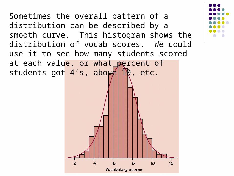
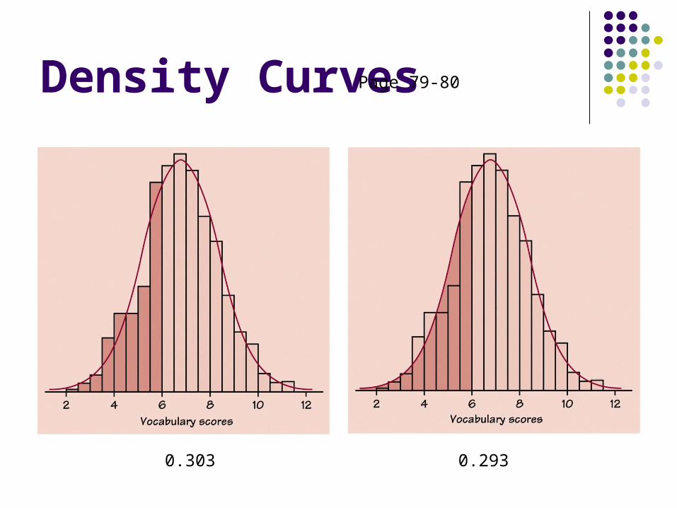
Sometimes the overall pattern of a distribution can be described by a smooth curve. This histogram shows the distribution of vocab scores. We could use it to see how many students scored at each value, or what percent of students got 4’s, above 10, etc.

Density CurvesA density curve is an idealized

mathematical model for a set of data.It ignores minor irregularities and

outliers

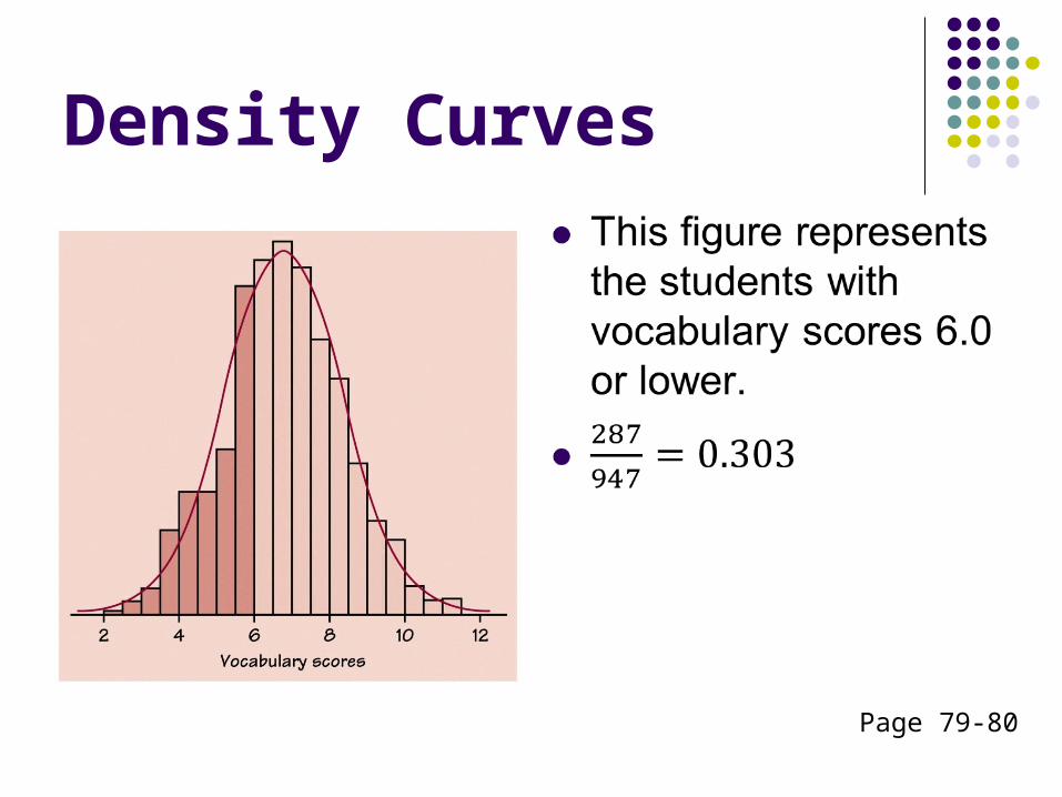
Density Curves

Page 79-80

Density Curves Page 79-80

0.303 0.293

Density Curve

Always on or above the horizontal axis

Has an area of exactly 1 underneath it

Types of Density CurvesNormal curvesUniform density curves

Later we’ll see important density curves that are skewed left/right and other curves related to the normal curve

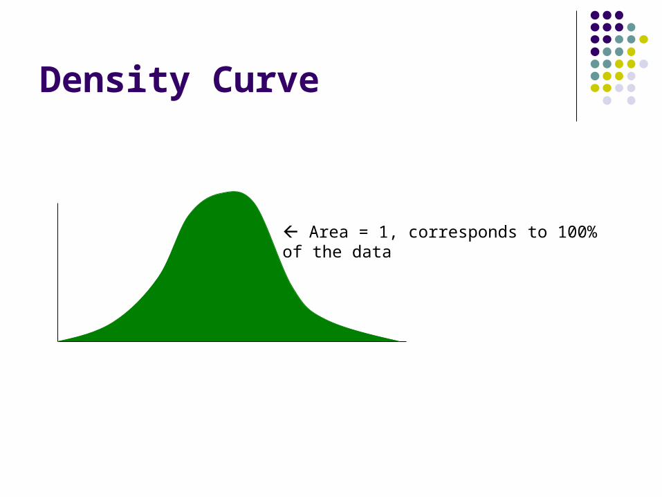
Density Curve

Area = 1, corresponds to 100% of the data

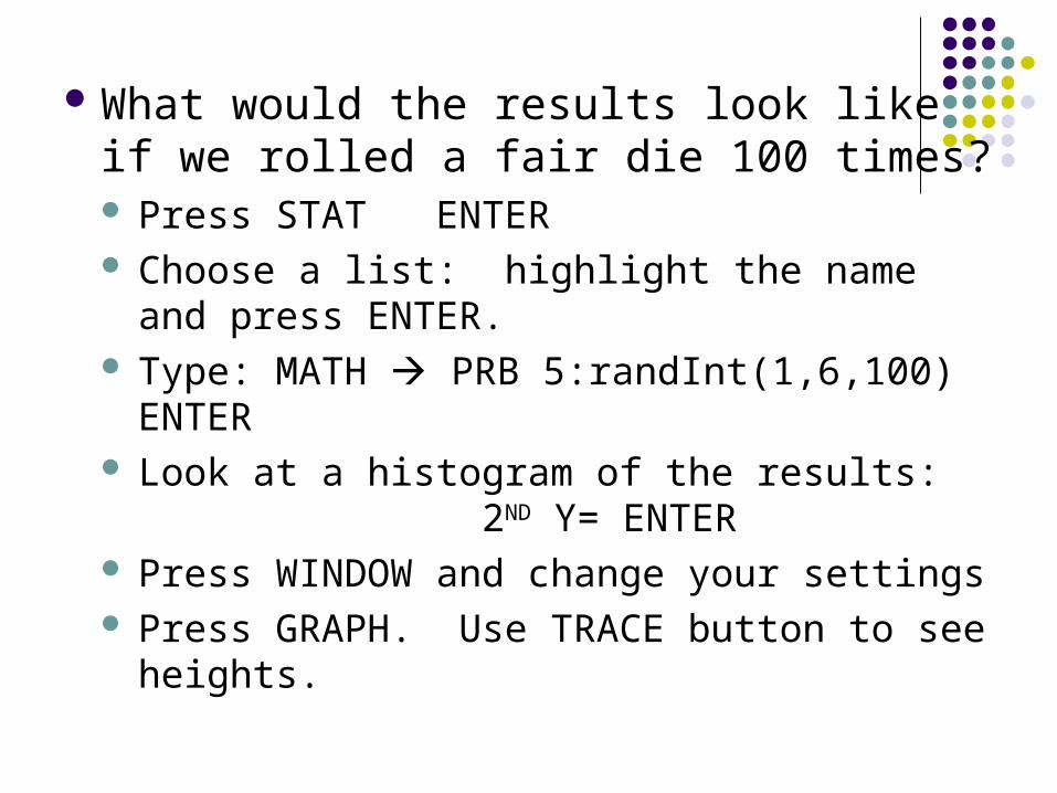
What would the results look like if we rolled a fair die 100 times? Press STAT ENTER Choose a list: highlight the name and press

ENTER. Type: MATH PRB 5:randInt(1,6,100)

ENTER Look at a histogram of the results:

2ND Y= ENTER Press WINDOW and change your settings Press GRAPH. Use TRACE button to see

heights.

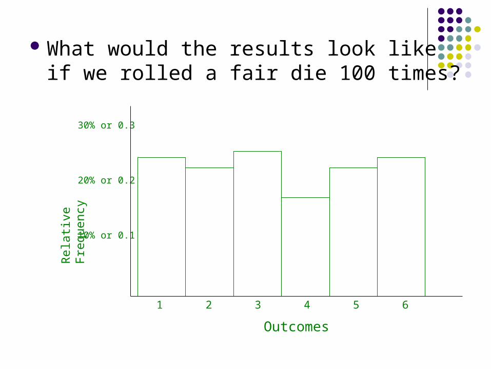
What would the results look like if we rolled a fair die 100 times?

1 2 3 4 5 6

Outcomes

30% or 0.3

20% or 0.2

10% or 0.1

Rela

tive F

req

uen

cy

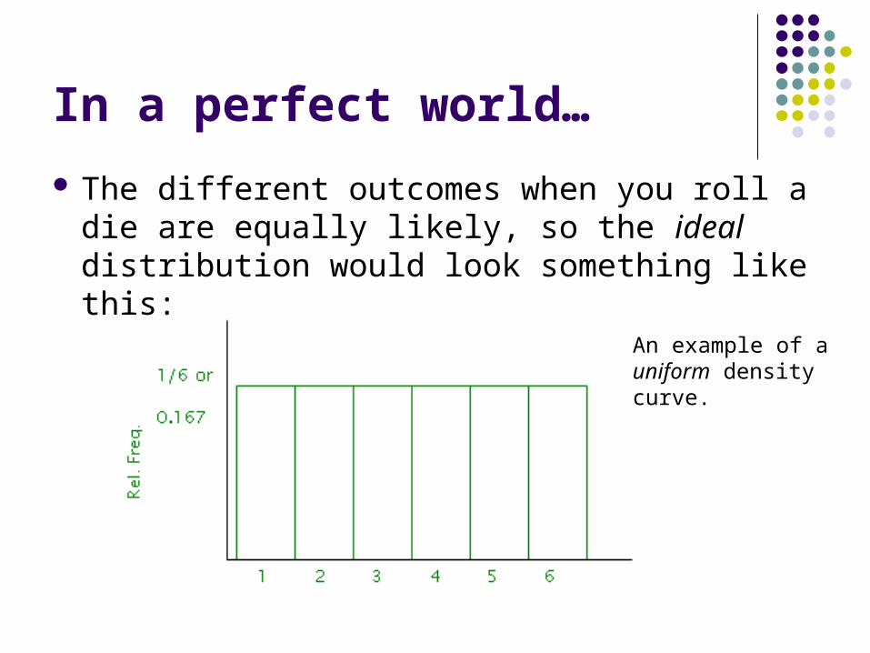
In a perfect world…

The different outcomes when you roll a die are equally likely, so the ideal distribution would look something like this:

An example of a uniform density curve.

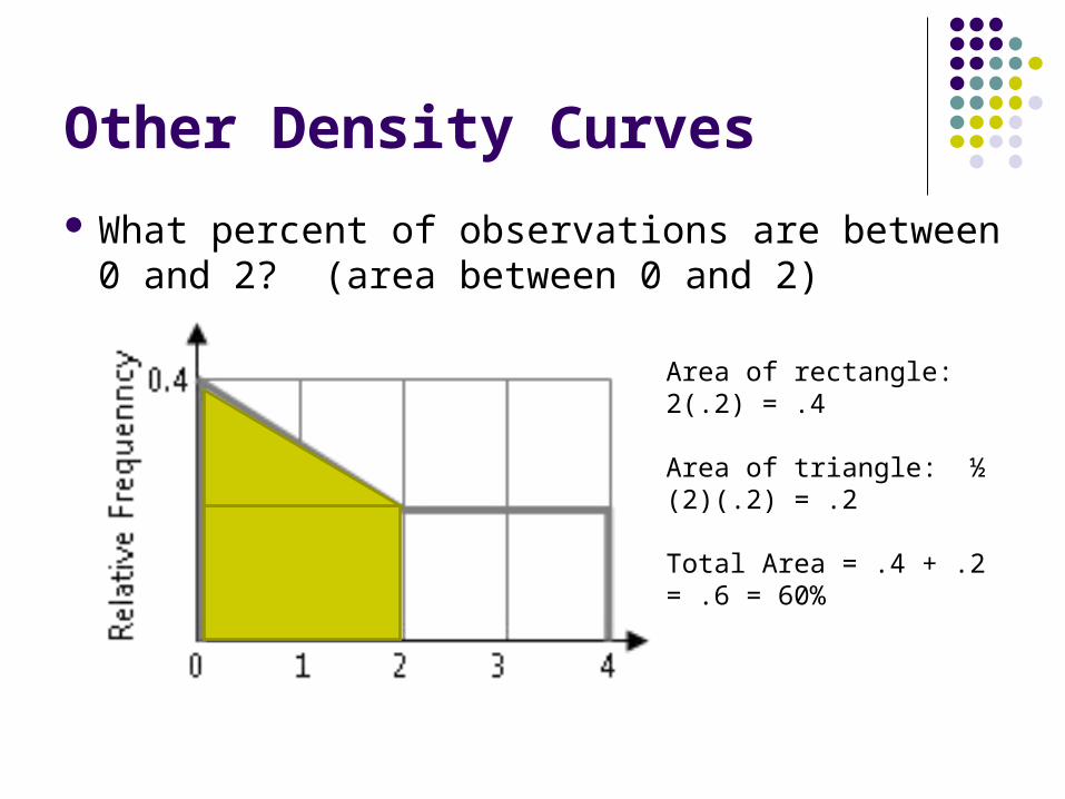
Other Density Curves

What percent of observations are between 0 and 2? (area between 0 and 2)

Area of rectangle: 2(.2) = .4

Area of triangle: ½ (2)(.2) = .2

Total Area = .4 + .2 = .6 = 60%

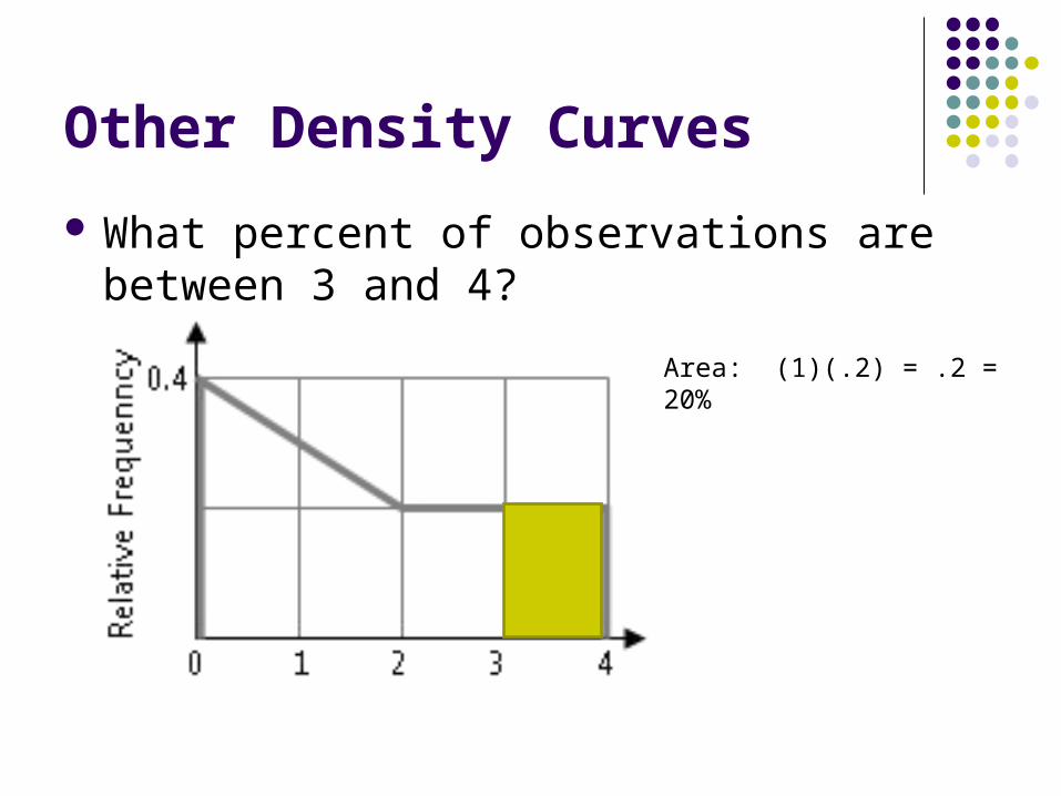
Other Density Curves

What percent of observations are between 3 and 4?

Area: (1)(.2) = .2 = 20%

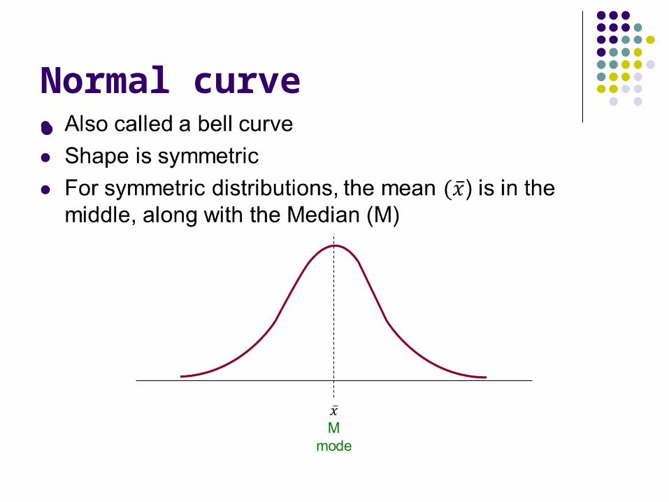
Normal curve

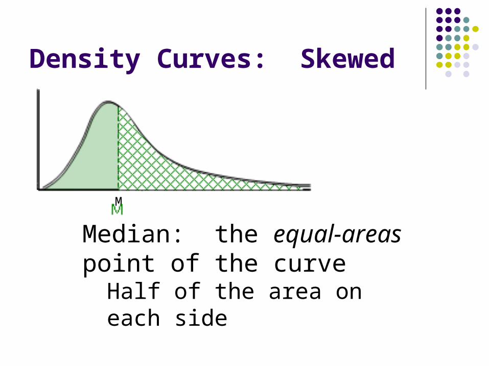
Density Curves: Skewed

Median: the equal-areas point of the curve

Half of the area on each side

M

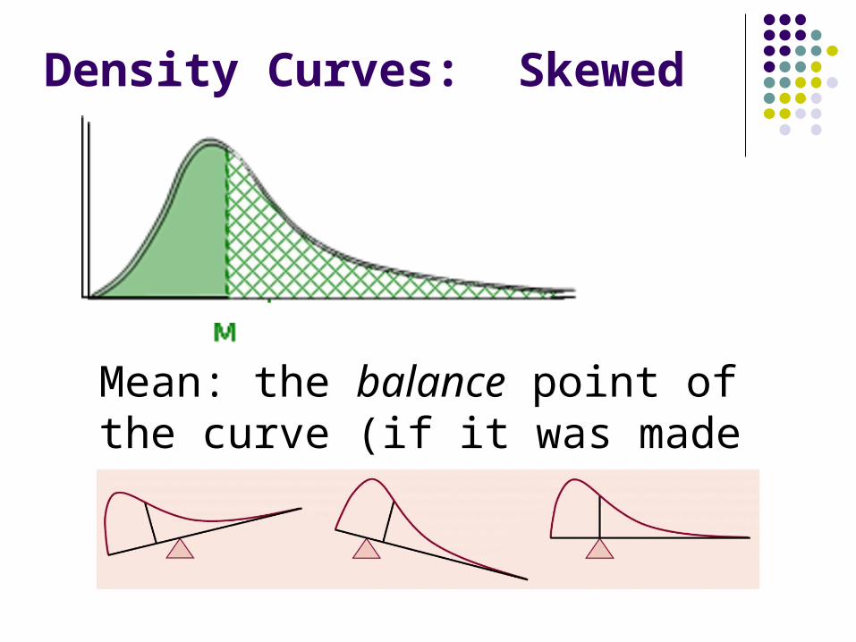
Density Curves: Skewed

Mean: the balance point of the curve (if it was made of solid material)

Mean and Median Of Density CurvesJust remember:Symmetrical distribution

Mean and median are in the centerSkewed distribution

Mean gets pulled towards the skew and away from the median.

Notation

Since density curves are idealized, the mean

and standard deviation of a density curve will

be slightly different from the actual mean and

standard deviation of the distribution

(histogram) that we’re approximating, and we

want a way to distinguish them

For actual observations (our sample): use and s.

For idealized (theoretical): use μ (mu) for mean and σ (sigma) for the standard deviation.

Notation

x

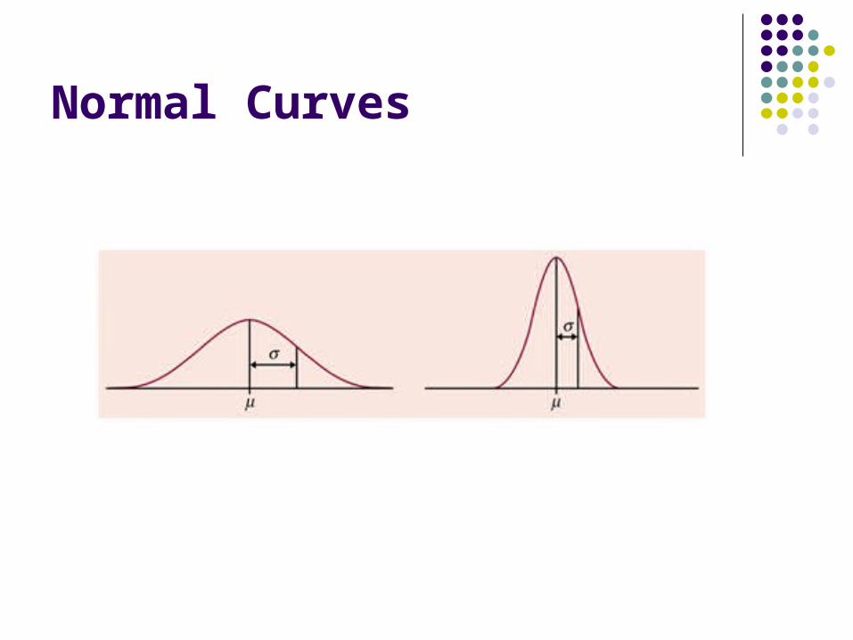
Normal Curves are always:

Described in terms of their mean (µ) and standard deviation (σ)

Symmetric

One peak and two tails

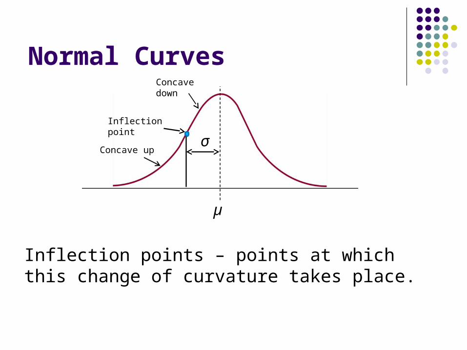
Normal Curves

Inflection points – points at which this change of curvature takes place.

µ

σ

Inflection point

Concave down

Concave up

Normal Curves

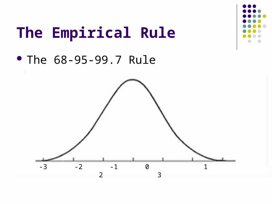
The Empirical Rule

The 68-95-99.7 Rule

-3 -2 -1 0 1 2 3

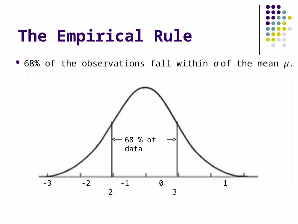
The Empirical Rule

68% of the observations fall within σ of the mean µ.

-3 -2 -1 0 1 2 3

68 % of data

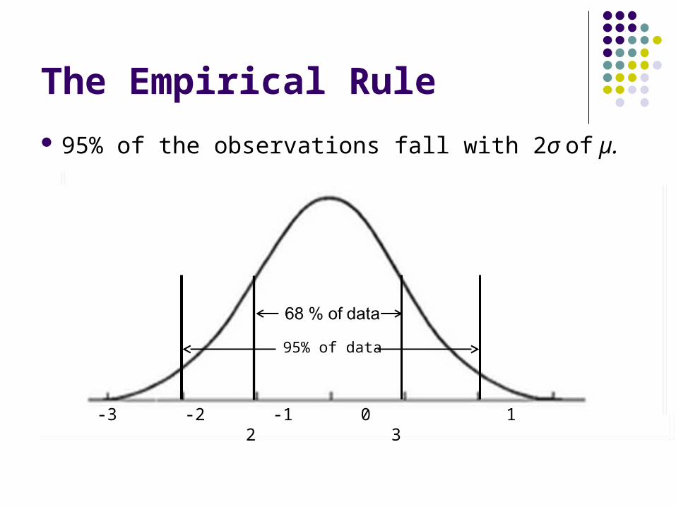
The Empirical Rule

95% of the observations fall with 2σ of µ.

-3 -2 -1 0 1 2 3

95% of data

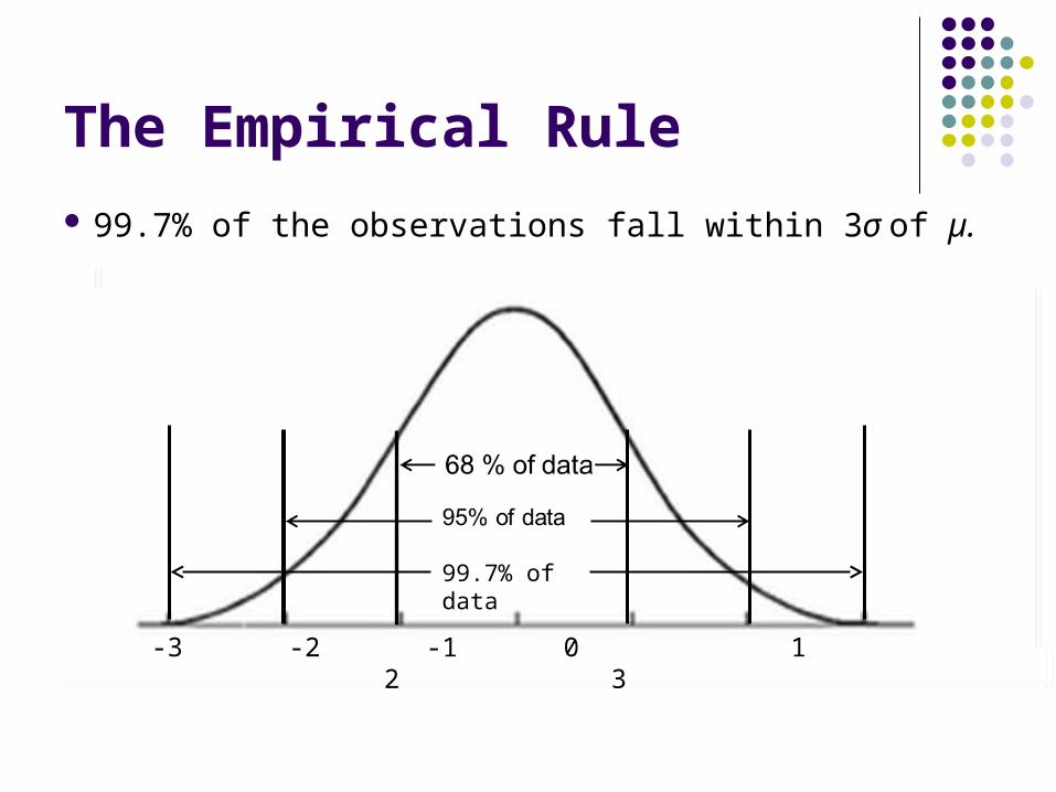
The Empirical Rule

99.7% of the observations fall within 3σ of µ.

-3 -2 -1 0 1 2 3

99.7% of data

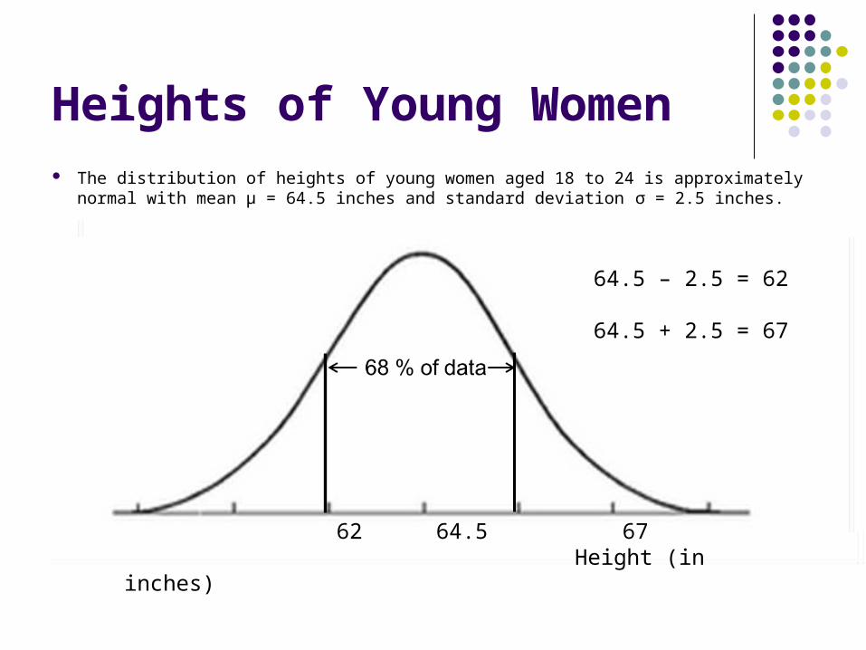
Heights of Young Women The distribution of heights of young women aged 18 to 24 is approximately

normal with mean µ = 64.5 inches and standard deviation σ = 2.5 inches.

62 64.5 67 Height (in inches)

64.5 – 2.5 = 62

64.5 + 2.5 = 67

Heights of Young Women The distribution of heights of young women aged 18 to 24 is approximately

normal with mean µ = 64.5 inches and standard deviation σ = 2.5 inches.

62 64.5 67 Height (in inches)

59.5 62 64.5 67 69.5 Height (in inches)

5

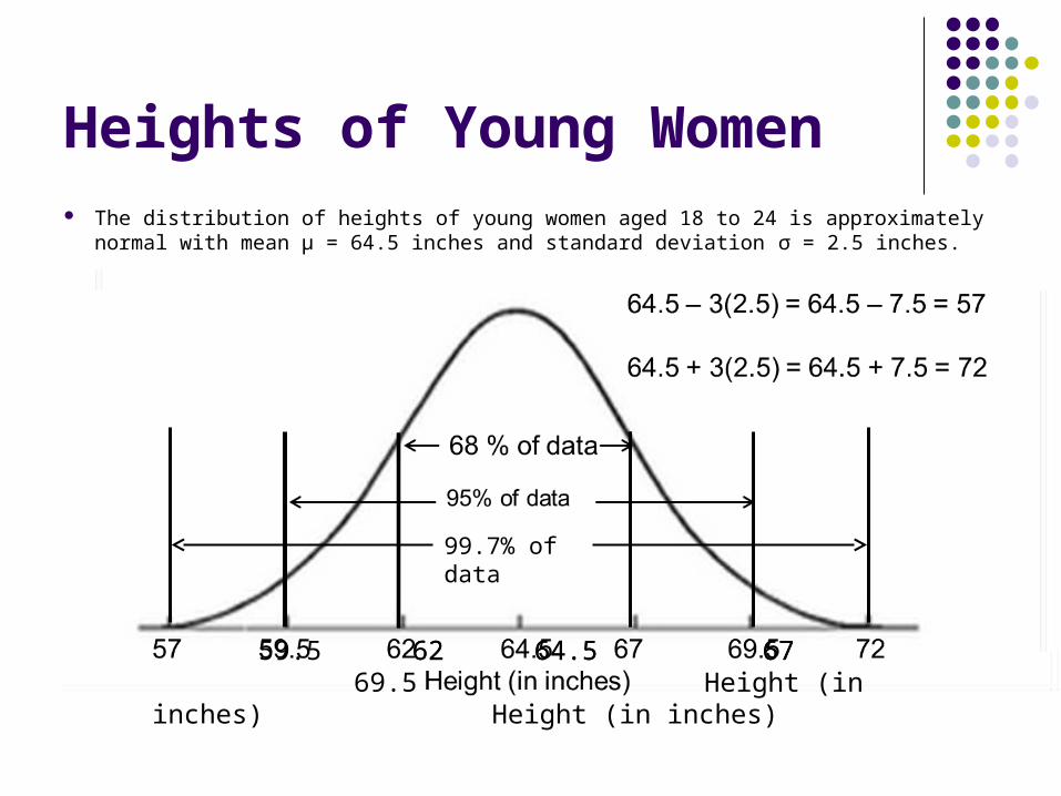
Heights of Young Women The distribution of heights of young women aged 18 to 24 is approximately

normal with mean µ = 64.5 inches and standard deviation σ = 2.5 inches.

62 64.5 67 Height (in inches)

59.5 62 64.5 67 69.5 Height (in inches)

99.7% of data

Shorthand with Normal Dist.

N(µ,σ)

Ex: The distribution of young women’s heights is N(64.5, 2.5).

What this means:

Normal Distribution centered at µ = 64.5 with a standard deviation σ = 2.5.

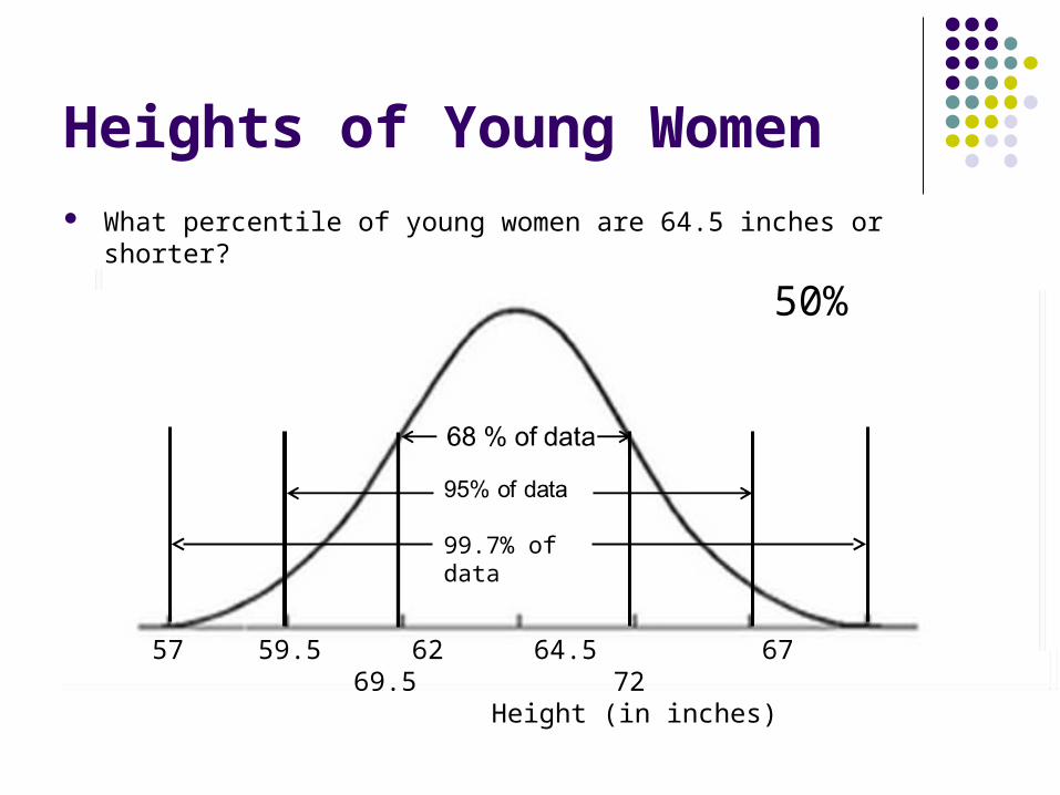
Heights of Young Women What percentile of young women are 64.5 inches or shorter?

57 59.5 62 64.5 67 69.5 72 Height (in inches)

99.7% of data

50%

Heights of Young Women What percentile of young women are 59.5 inches or shorter?

57 59.5 62 64.5 67 69.5 72 Height (in inches)

99.7% of data

2.5%

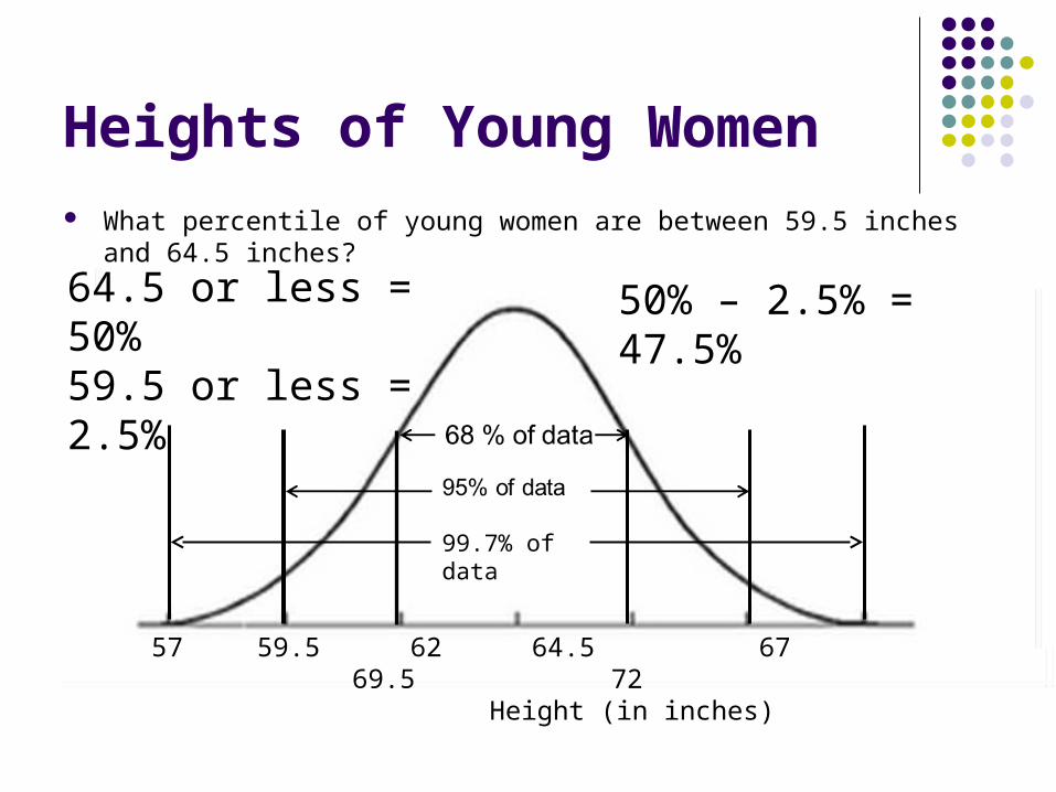
Heights of Young Women What percentile of young women are between 59.5 inches and 64.5 inches?

57 59.5 62 64.5 67 69.5 72 Height (in inches)

99.7% of data

64.5 or less = 50%59.5 or less = 2.5%

50% – 2.5% = 47.5%

For homework: 2.1, 2.3, 2.4 p. 83 2.6, 2.7, 2.8 p. 89

Practice