density-dependent selection and the limits of relative fitness

Density-dependent selection and the limits of relative

fitness

Jason Bertram 1,∗

Joanna Masel 1

1. Department of Ecology and Evolutionary Biology, University of Arizona, Tucson, AZ

85721.

∗ Corresponding author; e-mail: [email protected].

Keywords : Lottery model, competitive Lotka-Volterra, r/K-selection, interference com-

petition, eco-evo.

Author contributions : JB and JM conceptualized the manuscript. JB did the formal

analysis. JB wrote the manuscript with review and editing from JM.

Running title: Density-dependence and relative fitness

Acknowledgments : We thank Peter Chesson and Joachim Hermisson for many construc-

tive comments on an earlier and quite different version of this manuscript. This work was

financially supported by the National Science Foundation (DEB-1348262) and the John

Templeton Foundation (60814).

1

.CC-BY 4.0 International licenseIt is made available under a (which was not peer-reviewed) is the author/funder, who has granted bioRxiv a license to display the preprint in perpetuity.

The copyright holder for this preprint. http://dx.doi.org/10.1101/102087doi: bioRxiv preprint first posted online Jan. 21, 2017;

http://dx.doi.org/10.1101/102087

http://creativecommons.org/licenses/by/4.0/

Density-dependent selection and the1

limits of relative fitness2

Abstract3

Selection is commonly described by assigning constant relative fitness values to genotypes.4

Yet population density is often regulated by crowding. Relative fitness may then depend5

on density, and selection can change density when it acts on a density-regulating trait.6

When strong density-dependent selection acts on a density-regulating trait, selection is no7

longer describable by density-independent relative fitnesses, even in demographically stable8

populations. These conditions are met in most previous models of density-dependent selec-9

tion (e.g. “K-selection” in the logistic and Lotka-Volterra models), suggesting that density-10

independent relative fitnesses must be replaced with more ecologically explicit absolute fit-11

nesses unless selection is weak. Here we show that density-independent relative fitnesses12

can also accurately describe strong density-dependent selection under some conditions. We13

develop a novel model of density-regulated population growth with three ecologically intu-14

itive traits: fecundity, mortality, and competitive ability. Our model, unlike the logistic15

or Lotka-Volterra, incorporates a density-dependent juvenile “reproductive excess”, which16

largely decouples density-dependent selection from the regulation of density. We find that17

density-independent relative fitnesses accurately describe strong selection acting on any one18

trait, even fecundity, which is both density-regulating and subject to density-dependent se-19

lection. Our findings suggest that deviations from demographic equilibrium are the most20

serious threat to relative fitness models. In such cases our model offers a possible alternative21

to relative fitness.22

(210 words)23

2



http://dx.doi.org/10.1101/102087


Introduction24

There are a variety of different measures of fitness, such as expected lifetime reproductive25

ratio R0, intrinsic population growth rate r, equilibrium population density/carrying capac-26

ity (often labeled “K”) (Benton and Grant, 2000), and invasion fitness (Metz et al., 1992).27

In addition, “relative fitness” is widely used in evolutionary genetics, where the focus is on28

relative genotypic frequencies (Barton et al., 2007, pp. 468). The variety of fitness mea-29

sures is not problematic in itself, but it should be clear how these measures are connected30

to the processes of birth and death which ultimately drive selection (Metcalf and Pavard31

2007; Doebeli et al. 2017; Charlesworth 1994, pp. 178). While such a connection is clear32

for absolute fitness measures like r or R0, relative fitness has only weak justification from33

population ecology. It has even been proposed that relative fitness be justified from measure34

theory, abandoning population biology altogether (Wagner, 2010). Given the widespread use35

of relative fitness in evolutionary genetics, it is important to understand its population eco-36

logical basis, both to clarify its domain of applicability, and as part of the broader challenge37

of synthesizing ecology and evolution.38

For haploids tracked in discrete time, the change in the abundance ni of type i over a39

time step can be expressed as ∆ni = (Wi − 1)ni where Wi is “absolute fitness” (i.e. the40

abundance after one time step is n′i = Wini). The corresponding change in frequency is41

∆pi =(Wi

W− 1)pi, where W =

∑iWipi. In continuous time, the Malthusian parameter ri42

replaces Wi and we have dni

dt= rini and dpi

dt= (ri − r)pi (Crow et al., 1970). Note that43

we can replace the Wi with any set of values proportional to the Wi without affecting the44

ratio Wi/W or ∆pi. These “relative fitness” values tell us how type frequencies change,45

but give no information about the dynamics of total population density N =∑

i ni (Barton46

et al., 2007, pp. 468). Similarly in the continuous case, adding an arbitrary constant to the47

Malthusian parameters ri has no effect on dpidt

(these would then be relative log fitnesses).48

3



http://dx.doi.org/10.1101/102087


Relative fitness is often parameterized in terms of selection coefficients which represent49

the advantages of different types relative to each other. For instance, in continuous time50

s = r2− r1 is the selection coefficient of type 2 relative to type 1. Assuming that only 2 and51

1 are present, the change in frequency can be written as52

dp2

dt= sp2(1− p2). (1)

Thus, if r1 and r2 are constant, the frequency of the second type will grow logistically with53

a constant rate parameter s. We then say that selection is independent of frequency and54

density. The discrete time case is more complicated. Defining the selection coefficient by55

W2 = (1 + s)W1, and again assuming 1 and 2 are the only types present, we have56

∆p2 =W2 −W1

Wp2(1− p2) =

s

1 + sp2

p2(1− p2). (2)

Hence, even in the simplest case that W1 and W2 are constant, selection is frequency-57

dependent in discrete time (note that this frequency dependence is negligible when s is58

small compared to 1; see Frank 2011). We will refer to both the continuous and discrete59

time selection equations (1) and (2) throughout this paper, but the simpler continuous time60

case will be our point of comparison for the rest of this section.61

In a constant environment, and in the absence of crowding, ri is a constant “intrinsic”62

population growth rate. The interpretation of Eq. (1) is then simple: the selection coefficient63

s is simply the difference in intrinsic growth rates. However, growth cannot continue at a64

non-zero constant rate indefinitely: the population is not viable if ri < 0, whereas ri > 065

implies endlessly increasing population density. Thus, setting aside unviable populations,66

the increase in population density must be checked by crowding. This implies that the67

Malthusian parameters ri eventually decline to zero (e.g. Begon et al. 1990, pp. 203).68

Selection can then be density-dependent, and indeed this is probably not uncommon, because69

4



http://dx.doi.org/10.1101/102087


crowded and uncrowded conditions can favor very different traits (Travis et al., 2013). Eq. (1)70

is then not a complete description of selection — it lacks an additional coupled equation71

describing the dynamics of N , on which s in Eq. (1) now depends. In general we cannot72

simply specify the dynamics of N independently, because those ecological dynamics are73

coupled with the evolutionary dynamics of type frequency (Travis et al., 2013). Thus, in the74

presence of density-dependent selection, the simple procedure of assigning constant relative75

fitness values to different types has to be replaced with an ecological description of absolute76

growth rates. Note that frequency-dependent selection does not raise a similar problem,77

because a complete description of selection still only requires us to model the type frequencies,78

not the ecological variable N as well.79

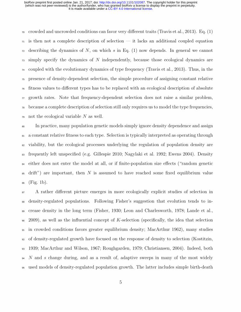
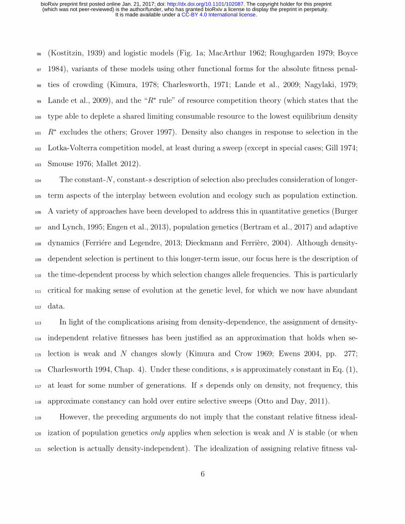
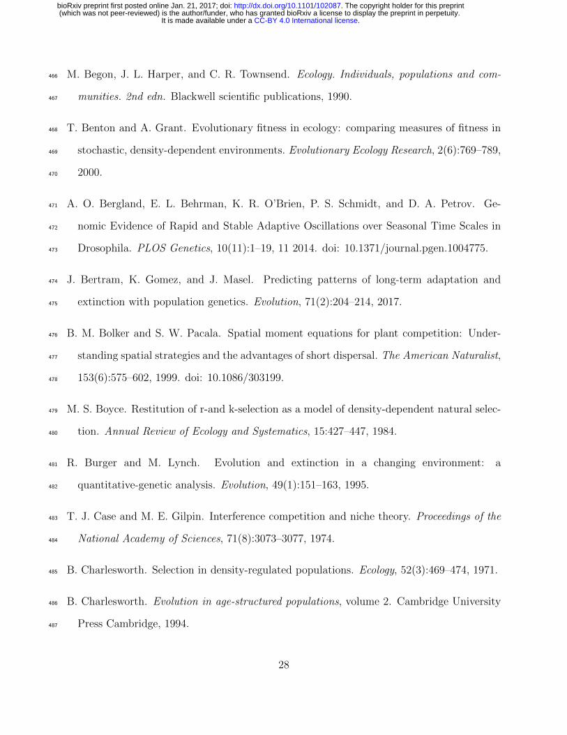
In practice, many population genetic models simply ignore density dependence and assign80

a constant relative fitness to each type. Selection is typically interpreted as operating through81

viability, but the ecological processes underlying the regulation of population density are82

frequently left unspecified (e.g. Gillespie 2010; Nagylaki et al. 1992; Ewens 2004). Density83

either does not enter the model at all, or if finite-population size effects (“random genetic84

drift”) are important, then N is assumed to have reached some fixed equilibrium value85

(Fig. 1b).86

A rather different picture emerges in more ecologically explicit studies of selection in87

density-regulated populations. Following Fisher’s suggestion that evolution tends to in-88

crease density in the long term (Fisher, 1930; Leon and Charlesworth, 1978; Lande et al.,89

2009), as well as the influential concept of K-selection (specifically, the idea that selection90

in crowded conditions favors greater equilibrium density; MacArthur 1962), many studies91

of density-regulated growth have focused on the response of density to selection (Kostitzin,92

1939; MacArthur and Wilson, 1967; Roughgarden, 1979; Christiansen, 2004). Indeed, both93

N and s change during, and as a result of, adaptive sweeps in many of the most widely94

used models of density-regulated population growth. The latter includes simple birth-death95

5



http://dx.doi.org/10.1101/102087


(Kostitzin, 1939) and logistic models (Fig. 1a; MacArthur 1962; Roughgarden 1979; Boyce96

1984), variants of these models using other functional forms for the absolute fitness penal-97

ties of crowding (Kimura, 1978; Charlesworth, 1971; Lande et al., 2009; Nagylaki, 1979;98

Lande et al., 2009), and the “R∗ rule” of resource competition theory (which states that the99

type able to deplete a shared limiting consumable resource to the lowest equilibrium density100

R∗ excludes the others; Grover 1997). Density also changes in response to selection in the101

Lotka-Volterra competition model, at least during a sweep (except in special cases; Gill 1974;102

Smouse 1976; Mallet 2012).103

The constant-N , constant-s description of selection also precludes consideration of longer-104

term aspects of the interplay between evolution and ecology such as population extinction.105

A variety of approaches have been developed to address this in quantitative genetics (Burger106

and Lynch, 1995; Engen et al., 2013), population genetics (Bertram et al., 2017) and adaptive107

dynamics (Ferriere and Legendre, 2013; Dieckmann and Ferriere, 2004). Although density-108

dependent selection is pertinent to this longer-term issue, our focus here is the description of109

the time-dependent process by which selection changes allele frequencies. This is particularly110

critical for making sense of evolution at the genetic level, for which we now have abundant111

data.112

In light of the complications arising from density-dependence, the assignment of density-113

independent relative fitnesses has been justified as an approximation that holds when se-114

lection is weak and N changes slowly (Kimura and Crow 1969; Ewens 2004, pp. 277;115

Charlesworth 1994, Chap. 4). Under these conditions, s is approximately constant in Eq. (1),116

at least for some number of generations. If s depends only on density, not frequency, this117

approximate constancy can hold over entire selective sweeps (Otto and Day, 2011).118

However, the preceding arguments do not imply that the constant relative fitness ideal-119

ization of population genetics only applies when selection is weak and N is stable (or when120

selection is actually density-independent). The idealization of assigning relative fitness val-121

6



http://dx.doi.org/10.1101/102087


n2

n1

dn1

dt= 0

dn2

dt= 0

K2

K1

(a)

n2

n1

dNdt

= 0

(b)

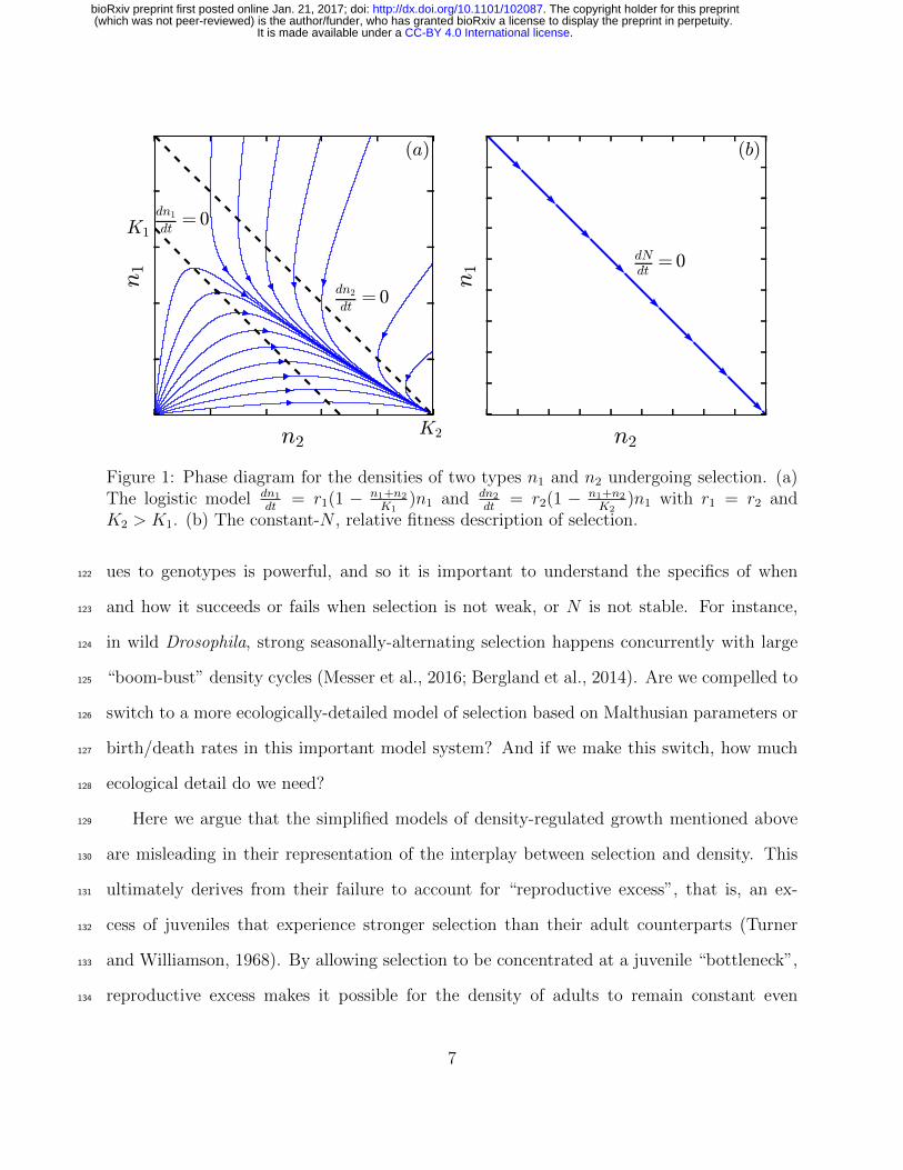
Figure 1: Phase diagram for the densities of two types n1 and n2 undergoing selection. (a)The logistic model dn1

dt= r1(1 − n1+n2

K1)n1 and dn2

dt= r2(1 − n1+n2

K2)n1 with r1 = r2 and

K2 > K1. (b) The constant-N , relative fitness description of selection.

ues to genotypes is powerful, and so it is important to understand the specifics of when122

and how it succeeds or fails when selection is not weak, or N is not stable. For instance,123

in wild Drosophila, strong seasonally-alternating selection happens concurrently with large124

“boom-bust” density cycles (Messer et al., 2016; Bergland et al., 2014). Are we compelled to125

switch to a more ecologically-detailed model of selection based on Malthusian parameters or126

birth/death rates in this important model system? And if we make this switch, how much127

ecological detail do we need?128

Here we argue that the simplified models of density-regulated growth mentioned above129

are misleading in their representation of the interplay between selection and density. This130

ultimately derives from their failure to account for “reproductive excess”, that is, an ex-131

cess of juveniles that experience stronger selection than their adult counterparts (Turner132

and Williamson, 1968). By allowing selection to be concentrated at a juvenile “bottleneck”,133

reproductive excess makes it possible for the density of adults to remain constant even134

7



http://dx.doi.org/10.1101/102087


under strong selection. Reproductive excess featured prominently in early debates about135

the regulation of population density (e.g. Nicholson 1954), and also has a long history in136

evolutionary theory, particularly related to Haldane’s “cost of selection” (Haldane, 1957;137

Turner and Williamson, 1968). Additionally, reproductive excess is implicit in foundational138

evolutionary-genetic models like the Wright-Fisher, where each generation involves the pro-139

duction of an infinite number of zygotes, of which a constant number N are sampled to form140

the next generation of adults. Likewise in the Moran model, a juvenile is always available to141

replace a dead adult every iteration no matter how rapidly adults are dying, and as a result142

N remains constant.143

Nevertheless, studies of density-dependent selection rarely incorporate reproductive ex-144

cess. This requires that we model a finite, density-dependent excess, which is substantially145

more complicated than modeling either zero (e.g. logistic) or infinite (e.g. Wright-Fisher)146

reproductive excess. Nei’s “competitive selection” model incorporated a finite reproductive147

excess to help clarify the “cost of selection” (Nei, 1971; Nagylaki et al., 1992), but used an148

unusual representation of competition based on pairwise interactions defined for at most two149

different genotypes, and was also restricted to equal fertilities for each genotype.150

In models with detailed age structure, it is usually assumed that the density of a “crit-151

ical age group” mediates the population’s response to crowding (Charlesworth, 1994, pp.152

54). Reproductive excess is a special case corresponding to a critical pre-reproductive age153

group. A central result of the theory of density-regulated age-structured populations is that154

selection proceeds in the direction of increasing equilibrium density in the critical age group155

(Charlesworth, 1994, pp. 148). This is a form of the classical K-selection ideas discussed156

above, but restricted to the critical age group (juveniles, in this case). The interdepen-157

dence of pre-reproductive selection and reproductive density is thus overlooked as a result158

of focusing on density in the critical age group.159

We re-evaluate the validity of the constant relative fitness description of selection in a160

8



http://dx.doi.org/10.1101/102087


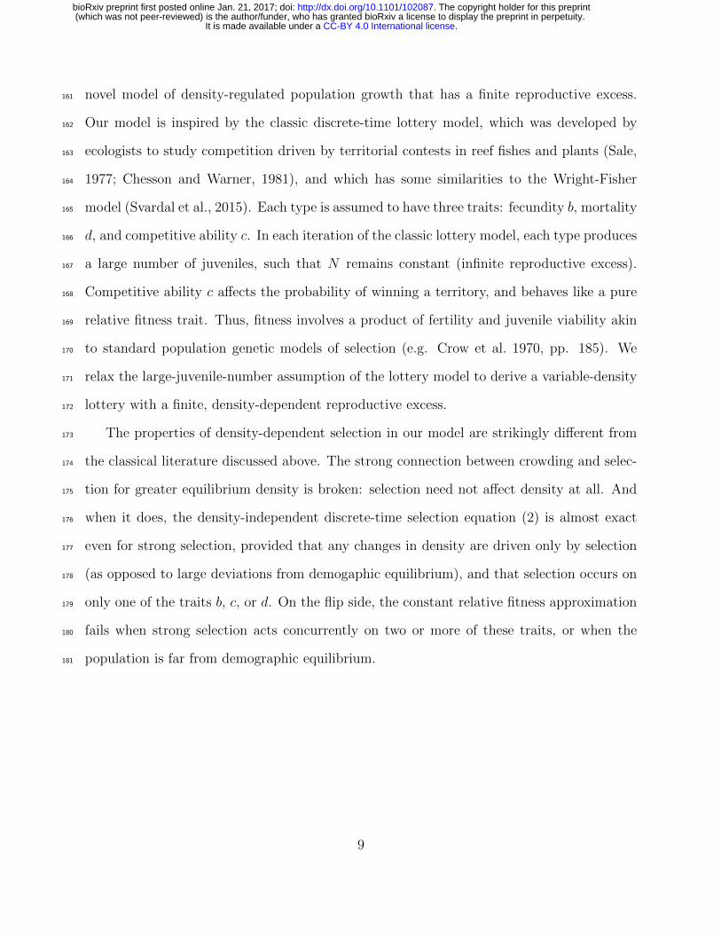
novel model of density-regulated population growth that has a finite reproductive excess.161

Our model is inspired by the classic discrete-time lottery model, which was developed by162

ecologists to study competition driven by territorial contests in reef fishes and plants (Sale,163

1977; Chesson and Warner, 1981), and which has some similarities to the Wright-Fisher164

model (Svardal et al., 2015). Each type is assumed to have three traits: fecundity b, mortality165

d, and competitive ability c. In each iteration of the classic lottery model, each type produces166

a large number of juveniles, such that N remains constant (infinite reproductive excess).167

Competitive ability c affects the probability of winning a territory, and behaves like a pure168

relative fitness trait. Thus, fitness involves a product of fertility and juvenile viability akin169

to standard population genetic models of selection (e.g. Crow et al. 1970, pp. 185). We170

relax the large-juvenile-number assumption of the lottery model to derive a variable-density171

lottery with a finite, density-dependent reproductive excess.172

The properties of density-dependent selection in our model are strikingly different from173

the classical literature discussed above. The strong connection between crowding and selec-174

tion for greater equilibrium density is broken: selection need not affect density at all. And175

when it does, the density-independent discrete-time selection equation (2) is almost exact176

even for strong selection, provided that any changes in density are driven only by selection177

(as opposed to large deviations from demogaphic equilibrium), and that selection occurs on178

only one of the traits b, c, or d. On the flip side, the constant relative fitness approximation179

fails when strong selection acts concurrently on two or more of these traits, or when the180

population is far from demographic equilibrium.181

9



http://dx.doi.org/10.1101/102087


Model182

Assumptions and definitions183

We restrict our attention to asexual haploids, since it is then clearer how the properties184

of selection are tied to the underlying population ecological assumptions. We assume that185

reproductively mature individuals (“adults”) require their own territory to survive and re-186

produce. All territories are identical, and the total number of territories is T . Time advances187

in discrete iterations, each representing the time from birth to reproductive maturity. In a188

given iteration, the number of adults of the i’th type will be denoted by ni, the total number189

of adults by N =∑

i ni, and the number of unoccupied territories by U = T−N . We assume190

that the ni are large enough that stochastic fluctuations in the ni (drift) can be ignored (with191

T also assumed large to allow for low type densities ni/T � 1).192

Each iteration, adults produce propagules which disperse at random, independently of193

distance from their parents, and independently of each other. We assume that each adult194

from type i produces bi propagules on average, so that the mean number of i propagules195

dispersing to unoccupied territories is mi = biniU/T . The parameter bi can be thought of as196

a measure of “colonization ability”, which combines fertility and dispersal ability (Levins and197

Culver, 1971; Tilman, 1994). Random dispersal is then modeled using a Poisson distribution198

pi(xi) = lxii e−li/xi! for the number xi of i propagules dispersing to any particular unoccupied199

territory, where li = mi/U is the mean propagule density in unoccupied territories. The200

total propagule density will be denoted L =∑

i li.201

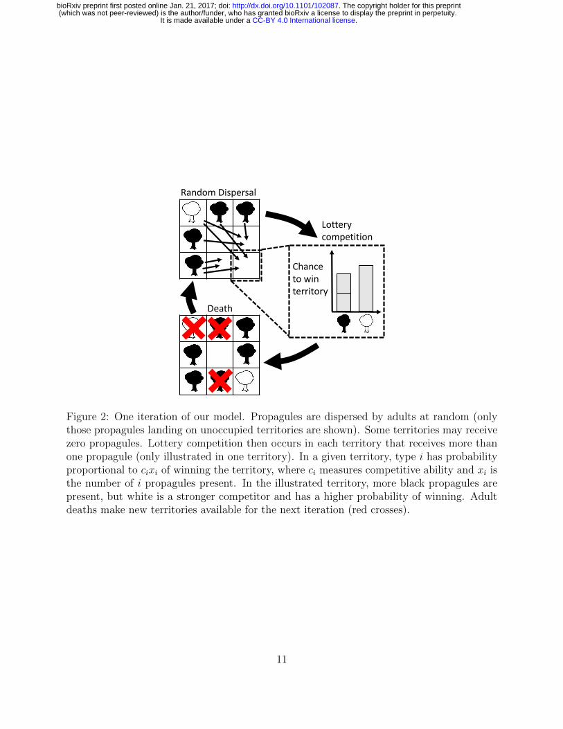
We assume that adults cannot be ousted by juveniles, so that recruitment to adulthood202

occurs exclusively in unoccupied territories. When multiple propagules land on the same203

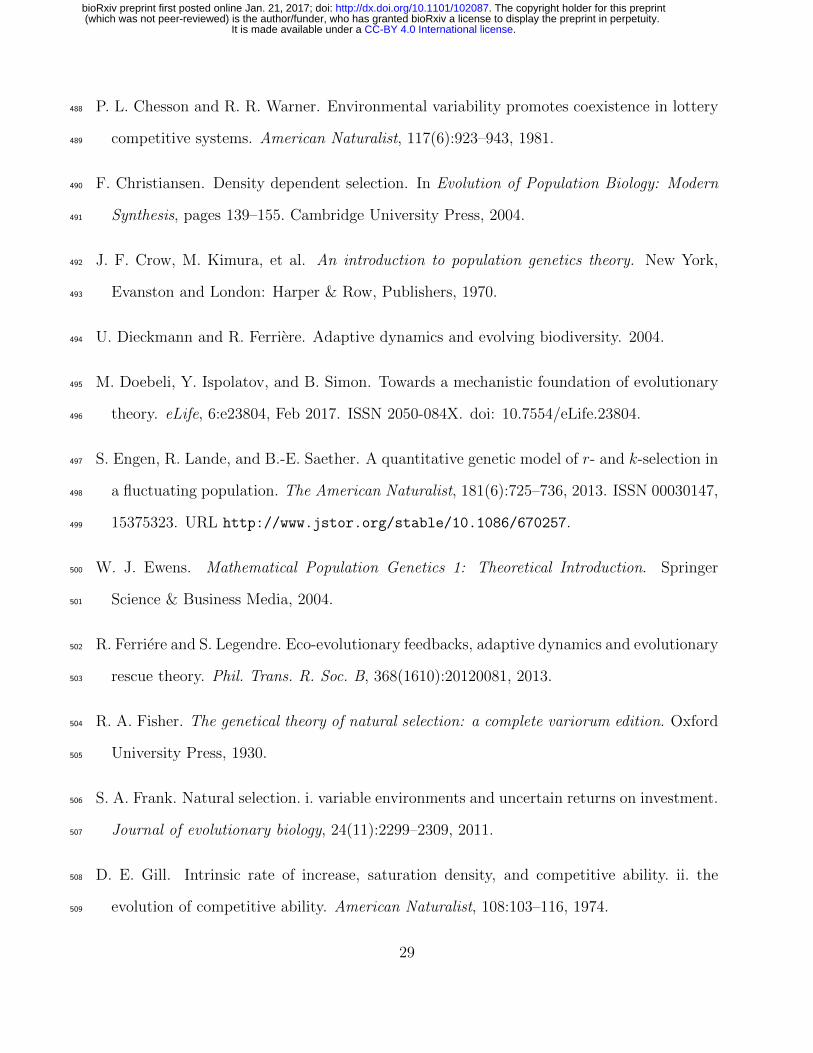
unoccupied territory, the winner is determined by lottery competition: type i wins a territory204

with probability cixi/∑

i cixi, where ci is a constant representing relative competitive ability205

(Fig. 2). Since the expected fraction of unoccupied territories with propagule composition206

10



http://dx.doi.org/10.1101/102087


Chance to win territory

Random Dispersal

Death

Lottery competition

Figure 2: One iteration of our model. Propagules are dispersed by adults at random (onlythose propagules landing on unoccupied territories are shown). Some territories may receivezero propagules. Lottery competition then occurs in each territory that receives more thanone propagule (only illustrated in one territory). In a given territory, type i has probabilityproportional to cixi of winning the territory, where ci measures competitive ability and xi isthe number of i propagules present. In the illustrated territory, more black propagules arepresent, but white is a stronger competitor and has a higher probability of winning. Adultdeaths make new territories available for the next iteration (red crosses).

11



http://dx.doi.org/10.1101/102087


x1, . . . , xG is p1(x1) · · · pG(xG) where G is the number of types present, and type i is expected207

to win a proportion cixi/∑

i cixi of these, type i’s expected territorial acquisition is given by208

∆+ni = U∑

x1,...,xG

cixi∑i cixi

p1(x1) · · · pG(xG). (3)

Here the sum only includes territories with at least one propagule present. Since we do not209

consider random genetic drift here, we will not analyze the fluctuations around these two210

expectations.211

Adult mortality occurs after lottery recruitment at a constant, type-specific per-capita212

rate di ≥ 1, and can affect adults recruited in the current iteration, such that the new213

abundance at the end of the iteration is (ni+∆+ni)/di (Fig. 2). In terms of absolute fitness,214

this can be written as215

Wi =1

di

(1 +

∆+nini

). (4)

Here ∆+ni

niis the per-capita rate of territorial acquisition, and 1/di is the fraction of type i216

adults surviving to the next iteration.217

Connection to the classic lottery model218

In the classic lottery model (Chesson and Warner, 1981), unoccupied territories are assumed219

to be saturated with propagules from every type (li → ∞ for all i). From the law of large220

numbers, the composition of propagules in each territory will not deviate appreciably from221

the mean composition l1, l2, . . . , lG. Type i is thus expected to win a proportion cili/∑

i cili222

of the U available territories,223

∆+ni =cili∑i cili

U =cilicL

U, (5)

12



http://dx.doi.org/10.1101/102087


where c =∑

i cimi/∑

imi is the mean competitive ability for a randomly selected propagule.224

Note that all unoccupied territories are filled in a single iteration of the classic lottery model,225

whereas our more general model Eq. (3) allows for territories to be left unoccupied and hence226

also accommodates low propagule densities.227

Results228

Analytical approximation of the variable-density lottery229

Here we evaluate the expectation in Eq. (3) to better understand the dynamics of density-230

dependent lottery competition. Similarly to the classic lottery model, we replace the xi,231

which take different values in different territories, with “effective” mean values. However,232

since we want to allow for low propagule densities, we cannot simply replace the xi with233

the means li as in the classic lottery. For a low density type, growth comes almost entirely234

from territories with xi = 1, for which its mean density li � 1 is not representative. We235

therefore separate Eq. (3) into xi = 1 and xi > 1 components, taking care to ensure that the236

effective mean approximations for these components are consistent with each other (details237

in Appendix B). The resulting variable-density approximation only requires that there are238

no large discrepancies in competitive ability (i.e. we do not have ci/cj � 1 for any two239

types). We obtain240

∆+ni ≈[e−L + (Ri + Ai)

cic

]liU, (6)

where241

Ri =ce−li(1− e−(L−li))

ci + cL−ciliL−li

L−1+e−L

1−(1+L)e−L

,

and242

Ai =c(1− e−li)

1−e−li

1−(1+li)e−licili + cL−cili

L−li

(L 1−e−L

1−(1+L)e−L − li 1−e−li

1−(1+li)e−li

) .13



http://dx.doi.org/10.1101/102087


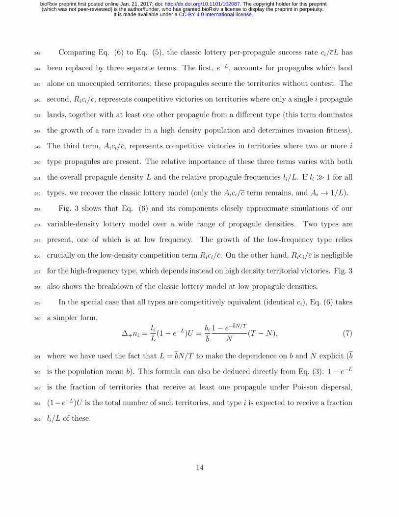
Comparing Eq. (6) to Eq. (5), the classic lottery per-propagule success rate ci/cL has243

been replaced by three separate terms. The first, e−L, accounts for propagules which land244

alone on unoccupied territories; these propagules secure the territories without contest. The245

second, Rici/c, represents competitive victories on territories where only a single i propagule246

lands, together with at least one other propagule from a different type (this term dominates247

the growth of a rare invader in a high density population and determines invasion fitness).248

The third term, Aici/c, represents competitive victories in territories where two or more i249

type propagules are present. The relative importance of these three terms varies with both250

the overall propagule density L and the relative propagule frequencies li/L. If li � 1 for all251

types, we recover the classic lottery model (only the Aici/c term remains, and Ai → 1/L).252

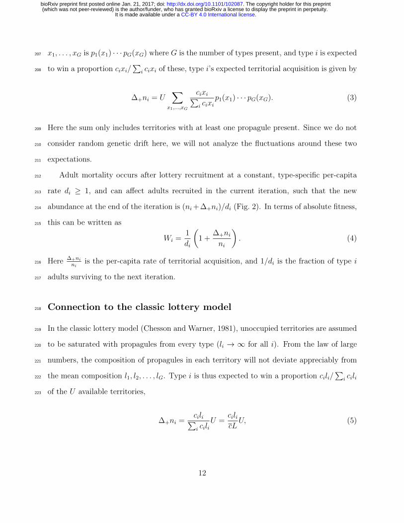
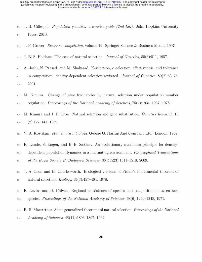
Fig. 3 shows that Eq. (6) and its components closely approximate simulations of our253

variable-density lottery model over a wide range of propagule densities. Two types are254

present, one of which is at low frequency. The growth of the low-frequency type relies255

crucially on the low-density competition term Rici/c. On the other hand, Rici/c is negligible256

for the high-frequency type, which depends instead on high density territorial victories. Fig. 3257

also shows the breakdown of the classic lottery model at low propagule densities.258

In the special case that all types are competitively equivalent (identical ci), Eq. (6) takes259

a simpler form,260

∆+ni =liL

(1− e−L)U =bi

b

1− e−bN/T

N(T −N), (7)

where we have used the fact that L = bN/T to make the dependence on b and N explicit (b261

is the population mean b). This formula can also be deduced directly from Eq. (3): 1− e−L262

is the fraction of territories that receive at least one propagule under Poisson dispersal,263

(1−e−L)U is the total number of such territories, and type i is expected to receive a fraction264

li/L of these.265

14



http://dx.doi.org/10.1101/102087


0 10 20L

0.0

0.2

0.4

0.6

0.8

1.0

Succ

ess

per

pro

pagule

Rare type

e−L

Ricic

Aicic

e−L +Ricic

+Aicic

Simulation

Classic lottery

0 10 20L

0.0

0.2

0.4

0.6

0.8

1.0

Common type

Figure 3: Comparison of Eq. (6), the classic lottery model, and simulations. The verticalaxis is per-propagule success rate for all propagules ∆+ni/mi, and for the three separatecomponents in Eq. (6). Two types are present with c1 = 1, c2 = 1.5 and l2/l1 = 0.1.Simulations are conducted as follows: x1, x2 values are sampled U = 105 times from Poissondistributions with respective means l1, l2, and the victorious type in each territory is thendecided by random sampling weighted by the lottery win probabilities cixi/(c1x1 + c2x2).Dashed lines show the failure of the classic lottery model at low density.

15



http://dx.doi.org/10.1101/102087


Similarly, the total number of territories acquired is266

∆+N = (1− e−L)U = (1− e−bN/T )(T −N) (8)

Density regulation and selection in the variable-density lottery267

Equipped with Eq. (6) we now outline the basic properties of the b, c and d traits. Adult268

density N is regulated by the birth and mortality rates b and d; b controls the fraction269

of unoccupied territories that are contested (see Eq. (8)), while d controls adult mortality.270

Competitive ability c does not enter Eq. (8), and therefore does not regulate total adult271

density: c only affects the relative likelihood of winning a contested territory.272

Selection in our variable-density lottery model is in general density-dependent, by which273

we mean that the discrete-time selection factor (W2 − W1)/W from Eq. (2) may depend274

on N . More specifically, as we show below, b- and c- selection are density-dependent, but275

d-selection is not. Note that density-dependent selection is sometimes taken to mean a276

qualitative change in which types are fitter than others at different densities (Travis et al.,277

2013). While reversal in the order of fitnesses and co-existence driven by density-regulation278

are possible in our variable-density lottery (a special case of the competition-colonization279

trade-off; Levins and Culver 1971; Tilman 1994; Bolker and Pacala 1999), questions related280

to co-existence are tangential to our aims and will not be pursued further here.281

The strength of b-selection declines with increasing density. When types differ in b only282

(b-selection), Eq. (6) simplifies to Eq. (7), and absolute fitness can be written as Wi =283

(1 + bibf(b,N))/di where f(b,N) = 1−e−bN/T

N(T − N) is a decreasing function of N . Thus,284

the selection factor W2−W1

W= f(b,N)

1+f(b,N)b2−b1b

declines with increasing density: the advantage of285

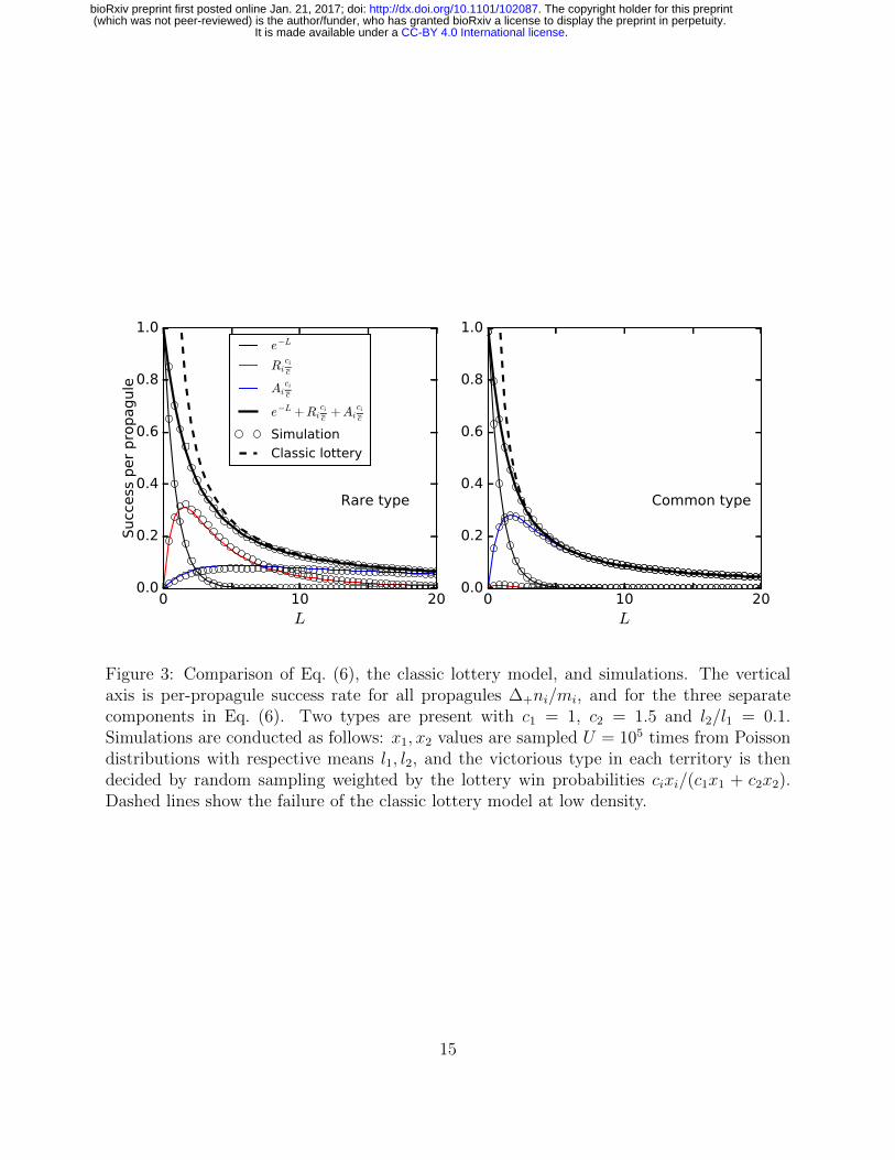
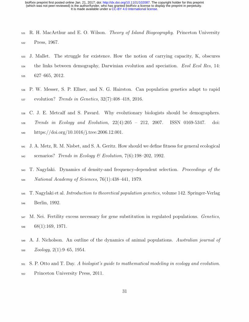
having greater b gets smaller the fewer territories there are to be claimed (Fig. 4).286

In the case of c-selection, Eq. (6) implies that W2 − W1 is proportional to287

T−NT

[(R2 + A2)c2 − (R1 + A1)c1] /c. The strength of c-selection thus peaks at an interme-288

16



http://dx.doi.org/10.1101/102087


0.0 0.2 0.4 0.6 0.8 1.0Density N/T

0.00

0.02

0.04

0.06

0.08

0.10

(W2−W

1)/W

b c d

Figure 4: The density-dependence of selection in our variable-density lottery between anadaptive variant 2 and a wildtype variant 1 with at equal frequencies. Here b1 = 1, d1 = 2 andc1 = 1. For b-selection we set b2 = b1(1+ε), and similarly for c and d, with ε = 0.1. d-selectionis density-independent, b-selection gets weaker with lower territorial availability, while c-selection initially increases with density as territorial contests become more important, buteventually also declines as available territories become scarce.

diate density (Fig. 4), because most territories are claimed without contest at low density289

(R1, R2, A1, A2 → 0), whereas at high density few unoccupied territories are available to be290

contested (T −N → 0).291

Selection on d is independent of density, because the density-dependent factor 1 + ∆+ni

ni292

in Eq. (4) is the same for types that differ in d only.293

The response of density to selection; c-selection versus K-selection294

We now turn to the issue of how density changes as a consequence of selection in our variable-295

density lottery, and in previous models of selection in density-regulated populations. In the296

latter, selection under crowded conditions typically induces changes in equilibrium density297

(see Introduction). In our variable-density lottery model, however, the competitive ability298

17



http://dx.doi.org/10.1101/102087


trait c is not density-regulating, even though c contributes to fitness under crowded condi-299

tions. Consequently, c-selection does not cause density to change. In this section we compare300

this c-selection behavior with the previous literature, which we take to be exemplified by301

MacArthur’s K-selection argument (MacArthur and Wilson, 1967).302

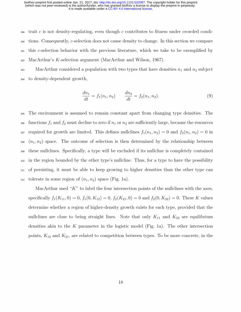
MacArthur considered a population with two types that have densities n1 and n2 subject303

to density-dependent growth,304

dn1

dt= f1(n1, n2)

dn2

dt= f2(n1, n2). (9)

The environment is assumed to remain constant apart from changing type densities. The305

functions f1 and f2 must decline to zero if n1 or n2 are sufficiently large, because the resources306

required for growth are limited. This defines nullclines f1(n1, n2) = 0 and f2(n1, n2) = 0 in307

(n1, n2) space. The outcome of selection is then determined by the relationship between308

these nullclines. Specifically, a type will be excluded if its nullcline is completely contained309

in the region bounded by the other type’s nullcline. Thus, for a type to have the possibility310

of persisting, it must be able to keep growing to higher densities than the other type can311

tolerate in some region of (n1, n2) space (Fig. 1a).312

MacArthur used “K” to label the four intersection points of the nullclines with the axes,

specifically f1(K11, 0) = 0, f1(0, K12) = 0, f2(K21, 0) = 0 and f2(0, K22) = 0. These K values

determine whether a region of higher-density growth exists for each type, provided that the

nullclines are close to being straight lines. Note that only K11 and K22 are equilibrium

densities akin to the K parameter in the logistic model (Fig. 1a). The other intersection

points, K12 and K21, are related to competition between types. To be more concrete, in the

18



http://dx.doi.org/10.1101/102087


n2

n1

K12 K22

K11

K21 (a)NullclinesN=K11 =K22

n2

n1

(b)

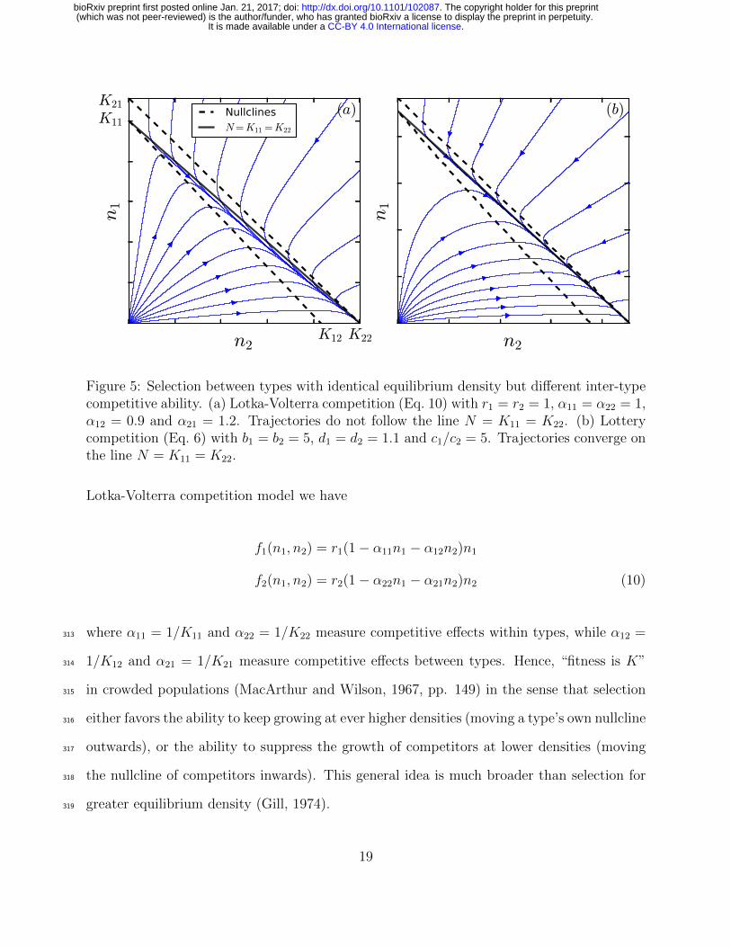
Figure 5: Selection between types with identical equilibrium density but different inter-typecompetitive ability. (a) Lotka-Volterra competition (Eq. 10) with r1 = r2 = 1, α11 = α22 = 1,α12 = 0.9 and α21 = 1.2. Trajectories do not follow the line N = K11 = K22. (b) Lotterycompetition (Eq. 6) with b1 = b2 = 5, d1 = d2 = 1.1 and c1/c2 = 5. Trajectories converge onthe line N = K11 = K22.

Lotka-Volterra competition model we have

f1(n1, n2) = r1(1− α11n1 − α12n2)n1

f2(n1, n2) = r2(1− α22n1 − α21n2)n2 (10)

where α11 = 1/K11 and α22 = 1/K22 measure competitive effects within types, while α12 =313

1/K12 and α21 = 1/K21 measure competitive effects between types. Hence, “fitness is K”314

in crowded populations (MacArthur and Wilson, 1967, pp. 149) in the sense that selection315

either favors the ability to keep growing at ever higher densities (moving a type’s own nullcline316

outwards), or the ability to suppress the growth of competitors at lower densities (moving317

the nullcline of competitors inwards). This general idea is much broader than selection for318

greater equilibrium density (Gill, 1974).319

19



http://dx.doi.org/10.1101/102087


Compared to simple birth-death models (Kostitzin, 1939) or variants of the logistic320

(Roughgarden, 1979), the Lotka-Volterra model clearly distinguishes between intra- and321

inter-type competitive effects. Thus, when selection acts on inter-type competitive effects,322

one type can displace another without having a greater equilibrium density (Fig. 5a). This323

has been termed “α-selection” to distinguish it from K-selection, which involves intra-type324

competitive effects and changes in equilibrium density Gill (1974); Joshi et al. (2001). Al-325

though the initial and final densities of an α-selection sweep are the same, density neverthe-326

less does change transiently in the Lotka-Volterra model (constant density only occurs for327

a highly restricted subset of r and α values; further details in Appendix C; also see Mallet328

2012; Smouse 1976). Intuitively, for one type to exclude the other, competitive suppression329

of growth between types must be stronger than competitive suppression of growth within330

types, causing N to dip over a sweep (Fig. 5a).331

In contrast to both K and α selection, density trajectories for c-selection in our variable-332

density lottery converge on a line of constant equilibrium density (Fig. 5b). This means333

that once N reaches demographic equilibrium, selective sweeps behave indistinguishably334

from a constant-N relative fitness model (Fig. 1b). Thus, for c sweeps, the selection factor335

(W2−W1)/W in Eq. (2) depends on frequency only, not density, provided that nothing else336

pushes N out of demographic equilibrium over the sweep. This uncoupling of density from337

ongoing c-selection arises due to the presence of an excess of propagules which pay the cost338

of selection without affecting adult density (Nei, 1971).339

Density-regulating traits and the threat of strong selection340

For the relative fitness model Eq. (2) to break down, the selection factor (W2 − W1)/W341

must depend on density. As shown in Fig. 4, (W2−W1)/W is independent of N in the case342

of d-selection. Selection is also independent of N when the population is at demographic343

equilibrium and N is unaffected by ongoing selection; as is the case for c-selection. Thus,344

20



http://dx.doi.org/10.1101/102087


to threaten Eq. (2), we require that selection is density-dependent, and also that density is345

changing. This can obviously occur if density-dependent selection happens in a population far346

from demographic equilibrium, in which case the validity of Eq. (2) depends on the specifics347

of the rate and magnitude of demographic change (we return to this in the Discussion).348

However, Eq. (2) can be threatened even in demographically-stable populations if a density-349

regulating trait is subject to density-dependent selection, as is the case for b in our variable-350

density lottery.351

Before we discuss the b trait, it is helpful to summarize how density-dependent selection352

on a density-regulating trait threatens Eq. (1) in simpler continuous-time models. This353

applies, for example, to K-selection in the logistic (Kimura and Crow, 1969; Crow et al.,354

1970). We consider the simple birth-death model (Kostitzin, 1939)355

dnidt

= (bi − δiN)ni, (11)

where δi is per-capita mortality due to crowding (for simplicity, there are no deaths when356

uncrowded). Starting from a type 1 population in equilibrium, a variant with δ2 = δ1(1− ε)357

has density-dependent selection coefficient s = εδ1N in Eq. (1), which will change over the358

course of the sweep as N shifts from its initial type 1 equilibrium to a type 2 equilibrium.359

From Eq. (11), the equilibrium densities at the beginning and end of the sweep are Ninitial =360

b1/δ1 and Nfinal = b1/(δ1(1 − ε)) = Ninitial/(1 − ε) respectively, and so sinitial = εb1 and361

sfinal = sinitial/(1 − ε). Consequently, substantial deviations from Eq. (1) occur if there is362

sufficiently strong selection on δ (Fig. 6).363

Equilibrium-to-equilibrium b-sweeps in our variable-density lottery are qualitatively dif-364

ferent from δ sweeps in this simpler birth-death model, because greater b not only means more365

propagules contesting territories, but also more territories being contested. Together, the366

net density-dependent effect on b-selection is negligible: in a single-type equilibrium we have367

21



http://dx.doi.org/10.1101/102087


0.0 0.1 0.2 0.3 0.4 0.5

ε

1.0

1.2

1.4

1.6

1.8

2.0s f

inal/s i

nitia

l(a)

Time0

1

Frequency

(b)

ε= 0. 2 (Eq. 11)

Canonical (Eq. 1)

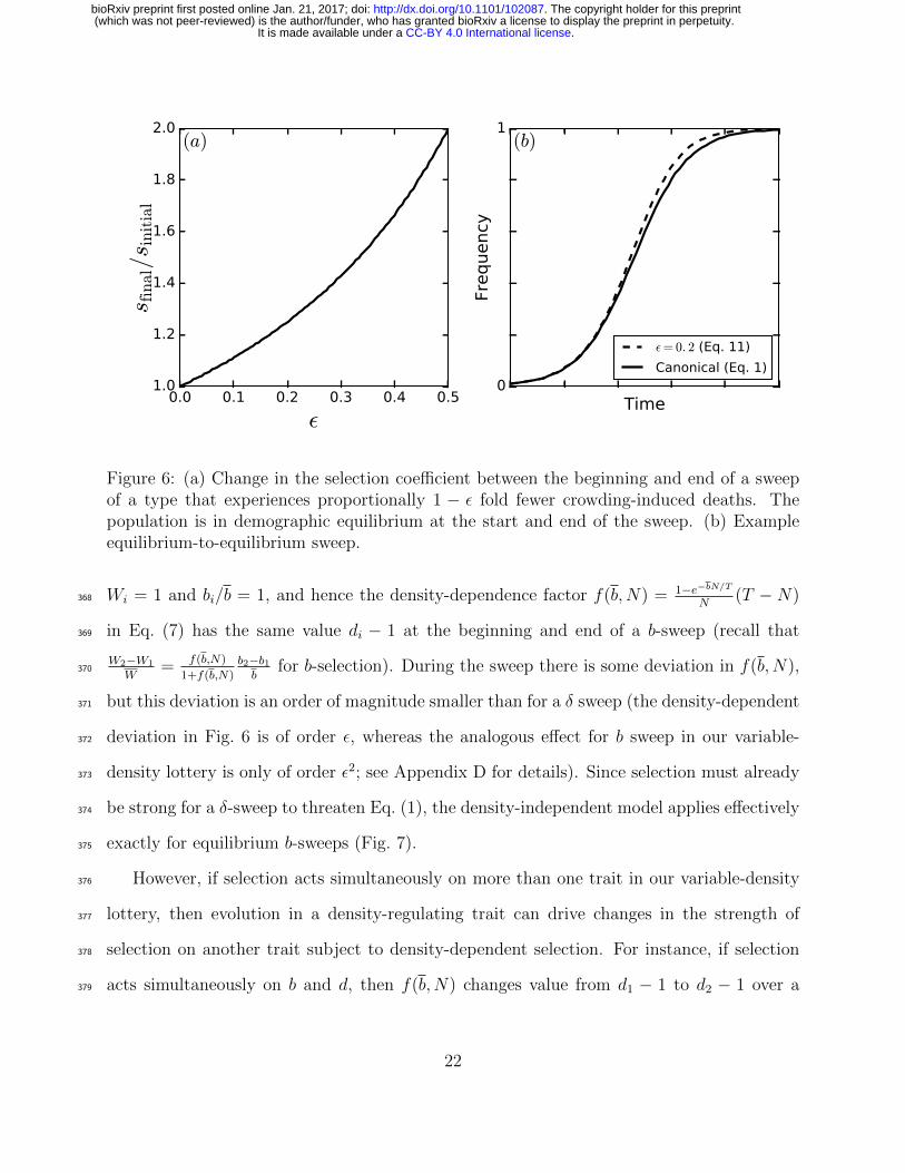
Figure 6: (a) Change in the selection coefficient between the beginning and end of a sweepof a type that experiences proportionally 1 − ε fold fewer crowding-induced deaths. Thepopulation is in demographic equilibrium at the start and end of the sweep. (b) Exampleequilibrium-to-equilibrium sweep.

Wi = 1 and bi/b = 1, and hence the density-dependence factor f(b,N) = 1−e−bN/T

N(T − N)368

in Eq. (7) has the same value di − 1 at the beginning and end of a b-sweep (recall that369

W2−W1

W= f(b,N)

1+f(b,N)b2−b1b

for b-selection). During the sweep there is some deviation in f(b,N),370

but this deviation is an order of magnitude smaller than for a δ sweep (the density-dependent371

deviation in Fig. 6 is of order ε, whereas the analogous effect for b sweep in our variable-372

density lottery is only of order ε2; see Appendix D for details). Since selection must already373

be strong for a δ-sweep to threaten Eq. (1), the density-independent model applies effectively374

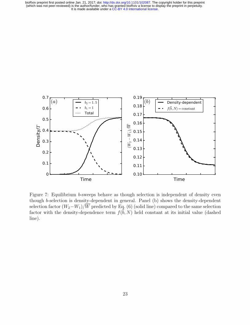
exactly for equilibrium b-sweeps (Fig. 7).375

However, if selection acts simultaneously on more than one trait in our variable-density376

lottery, then evolution in a density-regulating trait can drive changes in the strength of377

selection on another trait subject to density-dependent selection. For instance, if selection378

acts simultaneously on b and d, then f(b,N) changes value from d1 − 1 to d2 − 1 over a379

22



http://dx.doi.org/10.1101/102087


Time0

0.1

0.2

0.3

0.4

0.5

0.6

0.7

Densi

ty/T

(a) b2 = 1. 5

b1 = 1

Total

Time0.10

0.11

0.12

0.13

0.14

0.15

0.16

0.17

0.18

0.19

(W2−W

1)/W

(b) Density-dependent

f(b, N) = constant

Figure 7: Equilibrium b-sweeps behave as though selection is independent of density eventhough b-selection is density-dependent in general. Panel (b) shows the density-dependentselection factor (W2−W1)/W predicted by Eq. (6) (solid line) compared to the same selectionfactor with the density-dependence term f(b,N) held constant at its initial value (dashedline).

23



http://dx.doi.org/10.1101/102087


Time0

0.1

0.2

0.3

0.4

0.5

0.6

0.7

0.8D

ensi

ty/T

(a) b2 = 1. 25, d2 = 1. 4

b1 = 1, d1 = 1. 5

Total

Time0.11

0.12

0.13

0.14

0.15

0.16

0.17

0.18

(W2−W

1)/W

(b) Density-dependent

f(b, N) = constant

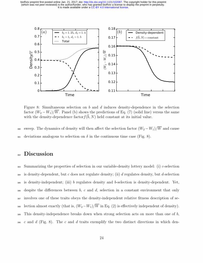
Figure 8: Simultaneous selection on b and d induces density-dependence in the selectionfactor (W2−W1)/W . Panel (b) shows the predictions of Eq. (7) (solid line) versus the samewith the density-dependence factorf(b,N) held constant at its initial value.

sweep. The dynamics of density will then affect the selection factor (W2−W1)/W and cause380

deviations analogous to selection on δ in the continuous time case (Fig. 8).381

Discussion382

Summarizing the properties of selection in our variable-density lottery model: (i) c-selection383

is density-dependent, but c does not regulate density; (ii) d regulates density, but d-selection384

is density-independent; (iii) b regulates density and b-selection is density-dependent. Yet,385

despite the differences between b, c and d, selection in a constant environment that only386

involves one of these traits obeys the density-independent relative fitness description of se-387

lection almost exactly (that is, (W2−W1)/W in Eq. (2) is effectively independent of density).388

This density-independence breaks down when strong selection acts on more than one of b,389

c and d (Fig. 8). The c and d traits exemplify the two distinct directions in which den-390

24



http://dx.doi.org/10.1101/102087


sity and selection can interact: selection may depend on density, and density may change391

in response to ongoing selection (Prout, 1980). The combination of both is necessary to392

threaten the constant-s approximation. Remarkably, the b trait demonstrates that the com-393

bination is not sufficient; the density-dependence of b-selection effectively disappears over394

equilibrium-to-equilibrium b-sweeps.395

Selection in the variable-density lottery is quite different from classical density-dependent396

selection (see “Introduction” and “The response of density to selection; c-selection versus397

K-selection”). In the latter, only one life-history stage is represented, and the effects of398

crowding appear as a reduction in absolute fitness that only depends on the type densities at399

this life-history stage (e.g. the n2i and ninj terms in the Lotka-Volterra equation). Selection400

in crowded populations takes broadly one of two forms: selection for greater carrying capacity401

(K-selection) or selection on competition coefficients (α-selection). These are both “δ-like”402

in the sense that selection depends on density and also causes density to change (δ is defined403

in Eq. (11)). Strong selection is therefore sufficient for Eq. (1) to break down (Fig. 6), and404

no distinction is made between density-regulating and density-dependent traits.405

The distinctive properties of selection in the variable-density lottery arise from a repro-406

ductive excess which appears when the number of propagules is greater than the number407

of available territories. Then only ≈ 1/L of the juveniles contesting unoccupied territories408

survive to adulthood. Unlike the role of adult density ni in single-life-stage models, it is409

the propagule densities li that represent the crowding that drives competition. Reproduc-410

tive excess produces relative contests in which fitter types grow at the expense of others by411

preferentially filling the available adult “slots”. The number of available slots can remain412

fixed or change independently of selection at the juvenile stage. By ignoring reproductive413

excess, single life-stage models are biased to have total population density be more sensi-414

tive to ongoing selection. In this respect, the viability selection heuristics that are common415

in population genetics (Gillespie, 2010, pp. 61) actually capture an important ecological416

25



http://dx.doi.org/10.1101/102087


process without making the full leap to complex age-structured models.417

Looking beyond the variable-density lottery, it is not clear which forms of crowding-418

induced selection are more likely to occur in nature. Even if reproductive excesses are419

ubiquitous, strictly relative c-like traits could pleiotropically interact with density-regulating420

traits so often that δ-like behavior is prevalent. For instance, in the case in the case of well-421

mixed indirect exploitation competition for consumable resources, the R∗ rule suggests that422

competitive ability is intimately linked to equilibrium resource density, and hence that δ-like423

behavior would be prevalent. However, this conclusion is sensititive to the assumptions of424

well-mixed resource competition models. Spatial localization of consumable resources (e.g.425

for plants due to restricted movement of nutrients through soils) will tend to create territorial426

contests similar to the lottery model, where resource competition only occurs locally and427

can be sensitive to contingencies such as the timing of propagule arrival (Bolker and Pacala,428

1999). In this case, resource competition is effectively subsumed into a territorial competitive429

ability trait akin to c, which would likely affect N much more weakly than suggested by the430

R∗ rule (assuming no pleiotropic interactions with b or d).431

Moreover, even in well-mixed populations, competition does not only involve indirect ex-432

ploitation of shared resources, but also direct interference. Interference competition can dra-433

matically alter the dynamics of resource exploitation (Case and Gilpin, 1974; Amarasekare,434

2002), and is more likely than the exploitation of shared resource pools to involve relative435

contests akin to c-selection. For instance, sexual selection can be viewed as a form of relative436

interference competition between genotypes. Thus, a priori we should not expect crowding437

in nature to only involve selection that is δ-like. Other forms of selection like c-selection (that438

is, strictly relative traits in density-regulated populations) are also likely to be important.439

Note that in the classical density-dependent selection literature, interference competition is440

closely associated with α-selection and the idea that selection need not affect equilibrium441

density (Gill, 1974). However, α-selection does transiently affect population density and442

26



http://dx.doi.org/10.1101/102087


therefore retains δ-like features.443

The above findings underscore that the most serious threat to the density-independent444

models of selection (Eqs. (1) and (2)) arises due to deviations from demographic equilibrium445

as a result of changes in the demographic rates of the types already present i.e. as a result446

of a temporally-variable environment. While transient deviations from demographic equi-447

librium driven by the appearance of new types can also threaten the density-independent448

approximation, this requires strong selection that is both density-dependent and affects a449

density-regulating trait (and, as exemplified by b-selection, even then the approximation450

may hold). By contrast, temporally-variable environments can dramatically alter frequency451

trajectories for individual sweeps (e.g. Fig. 9.5 in Otto and Day (2011); Fig. 5 in Mallet452

(2012)), as well as the long-term outcomes of selection (Lande et al., 2009).453

This suggests that in systems like the wild Drosophila example mentioned in the Intro-454

duction, there may indeed be no choice but to abandon relative fitness. Our variable-density455

lottery could provide a useful starting point for analyzing evolution in this and other far-456

from-equilibrium situations for two reasons: 1) the b, c, d trait scheme neatly distinguishes457

between different aspects of the interplay between density and selection; 2) lottery models in458

general are mathematically similar to the Wright-Fisher model, which should facilitate the459

analysis of genetic drift when N is unstable.460

References461

P. Amarasekare. Interference competition and species coexistence. Proceedings of the Royal462

Society of London B: Biological Sciences, 269(1509):2541–2550, 2002.463

N. Barton, D. Briggs, J. Eisen, D. Goldstein, and N. Patel. Evolution. NY: Cold Spring464

Harbor Laboratory Press, 2007.465

27



http://dx.doi.org/10.1101/102087


M. Begon, J. L. Harper, and C. R. Townsend. Ecology. Individuals, populations and com-466

munities. 2nd edn. Blackwell scientific publications, 1990.467

T. Benton and A. Grant. Evolutionary fitness in ecology: comparing measures of fitness in468

stochastic, density-dependent environments. Evolutionary Ecology Research, 2(6):769–789,469

2000.470

A. O. Bergland, E. L. Behrman, K. R. O’Brien, P. S. Schmidt, and D. A. Petrov. Ge-471

nomic Evidence of Rapid and Stable Adaptive Oscillations over Seasonal Time Scales in472

Drosophila. PLOS Genetics, 10(11):1–19, 11 2014. doi: 10.1371/journal.pgen.1004775.473

J. Bertram, K. Gomez, and J. Masel. Predicting patterns of long-term adaptation and474

extinction with population genetics. Evolution, 71(2):204–214, 2017.475

B. M. Bolker and S. W. Pacala. Spatial moment equations for plant competition: Under-476

standing spatial strategies and the advantages of short dispersal. The American Naturalist,477

153(6):575–602, 1999. doi: 10.1086/303199.478

M. S. Boyce. Restitution of r-and k-selection as a model of density-dependent natural selec-479

tion. Annual Review of Ecology and Systematics, 15:427–447, 1984.480

R. Burger and M. Lynch. Evolution and extinction in a changing environment: a481

quantitative-genetic analysis. Evolution, 49(1):151–163, 1995.482

T. J. Case and M. E. Gilpin. Interference competition and niche theory. Proceedings of the483

National Academy of Sciences, 71(8):3073–3077, 1974.484

B. Charlesworth. Selection in density-regulated populations. Ecology, 52(3):469–474, 1971.485

B. Charlesworth. Evolution in age-structured populations, volume 2. Cambridge University486

Press Cambridge, 1994.487

28



http://dx.doi.org/10.1101/102087


P. L. Chesson and R. R. Warner. Environmental variability promotes coexistence in lottery488

competitive systems. American Naturalist, 117(6):923–943, 1981.489

F. Christiansen. Density dependent selection. In Evolution of Population Biology: Modern490

Synthesis, pages 139–155. Cambridge University Press, 2004.491

J. F. Crow, M. Kimura, et al. An introduction to population genetics theory. New York,492

Evanston and London: Harper & Row, Publishers, 1970.493

U. Dieckmann and R. Ferriere. Adaptive dynamics and evolving biodiversity. 2004.494

M. Doebeli, Y. Ispolatov, and B. Simon. Towards a mechanistic foundation of evolutionary495

theory. eLife, 6:e23804, Feb 2017. ISSN 2050-084X. doi: 10.7554/eLife.23804.496

S. Engen, R. Lande, and B.-E. Saether. A quantitative genetic model of r- and k-selection in497

a fluctuating population. The American Naturalist, 181(6):725–736, 2013. ISSN 00030147,498

15375323. URL http://www.jstor.org/stable/10.1086/670257.499

W. J. Ewens. Mathematical Population Genetics 1: Theoretical Introduction. Springer500

Science & Business Media, 2004.501

R. Ferriere and S. Legendre. Eco-evolutionary feedbacks, adaptive dynamics and evolutionary502

rescue theory. Phil. Trans. R. Soc. B, 368(1610):20120081, 2013.503

R. A. Fisher. The genetical theory of natural selection: a complete variorum edition. Oxford504

University Press, 1930.505

S. A. Frank. Natural selection. i. variable environments and uncertain returns on investment.506

Journal of evolutionary biology, 24(11):2299–2309, 2011.507

D. E. Gill. Intrinsic rate of increase, saturation density, and competitive ability. ii. the508

evolution of competitive ability. American Naturalist, 108:103–116, 1974.509

29



http://dx.doi.org/10.1101/102087


J. H. Gillespie. Population genetics: a concise guide (2nd Ed.). John Hopkins University510

Press, 2010.511

J. P. Grover. Resource competition, volume 19. Springer Science & Business Media, 1997.512

J. B. S. Haldane. The cost of natural selection. Journal of Genetics, 55(3):511, 1957.513

A. Joshi, N. Prasad, and M. Shakarad. K-selection, α-selection, effectiveness, and tolerance514

in competition: density-dependent selection revisited. Journal of Genetics, 80(2):63–75,515

2001.516

M. Kimura. Change of gene frequencies by natural selection under population number517

regulation. Proceedings of the National Academy of Sciences, 75(4):1934–1937, 1978.518

M. Kimura and J. F. Crow. Natural selection and gene substitution. Genetics Research, 13519

(2):127–141, 1969.520

V. A. Kostitzin. Mathematical biology. George G. Harrap And Company Ltd.; London, 1939.521

R. Lande, S. Engen, and B.-E. Sæther. An evolutionary maximum principle for density-522

dependent population dynamics in a fluctuating environment. Philosophical Transactions523

of the Royal Society B: Biological Sciences, 364(1523):1511–1518, 2009.524

J. A. Leon and B. Charlesworth. Ecological versions of Fisher’s fundamental theorem of525

natural selection. Ecology, 59(3):457–464, 1978.526

R. Levins and D. Culver. Regional coexistence of species and competition between rare527

species. Proceedings of the National Academy of Sciences, 68(6):1246–1248, 1971.528

R. H. MacArthur. Some generalized theorems of natural selection. Proceedings of the National529

Academy of Sciences, 48(11):1893–1897, 1962.530

30



http://dx.doi.org/10.1101/102087


R. H. MacArthur and E. O. Wilson. Theory of Island Biogeography. Princeton University531

Press, 1967.532

J. Mallet. The struggle for existence. How the notion of carrying capacity, K, obscures533

the links between demography, Darwinian evolution and speciation. Evol Ecol Res, 14:534

627–665, 2012.535

P. W. Messer, S. P. Ellner, and N. G. Hairston. Can population genetics adapt to rapid536

evolution? Trends in Genetics, 32(7):408–418, 2016.537

C. J. E. Metcalf and S. Pavard. Why evolutionary biologists should be demographers.538

Trends in Ecology and Evolution, 22(4):205 – 212, 2007. ISSN 0169-5347. doi:539

https://doi.org/10.1016/j.tree.2006.12.001.540

J. A. Metz, R. M. Nisbet, and S. A. Geritz. How should we define fitness for general ecological541

scenarios? Trends in Ecology & Evolution, 7(6):198–202, 1992.542

T. Nagylaki. Dynamics of density-and frequency-dependent selection. Proceedings of the543

National Academy of Sciences, 76(1):438–441, 1979.544

T. Nagylaki et al. Introduction to theoretical population genetics, volume 142. Springer-Verlag545

Berlin, 1992.546

M. Nei. Fertility excess necessary for gene substitution in regulated populations. Genetics,547

68(1):169, 1971.548

A. J. Nicholson. An outline of the dynamics of animal populations. Australian journal of549

Zoology, 2(1):9–65, 1954.550

S. P. Otto and T. Day. A biologist’s guide to mathematical modeling in ecology and evolution.551

Princeton University Press, 2011.552

31



http://dx.doi.org/10.1101/102087


T. Prout. Some relationships between density-independent selection and density-dependent553

population growth. Evol. Biol, 13:1–68, 1980.554

J. Roughgarden. Theory of population genetics and evolutionary ecology: an introduction.555

Macmillan New York NY United States, 1979.556

P. F. Sale. Maintenance of high diversity in coral reef fish communities. The American557

Naturalist, 111(978):337–359, 1977.558

P. E. Smouse. The implications of density-dependent population growth for frequency-and559

density-dependent selection. The American Naturalist, 110(975):849–860, 1976.560

H. Svardal, C. Rueffler, and J. Hermisson. A general condition for adaptive genetic polymor-561

phism in temporally and spatially heterogeneous environments. Theoretical Population Bi-562

ology, 99:76 – 97, 2015. ISSN 0040-5809. doi: http://dx.doi.org/10.1016/j.tpb.2014.11.002.563

D. Tilman. Competition and biodiversity in spatially structured habitats. Ecology, 75(1):564

2–16, 1994.565

J. Travis, J. Leips, and F. H. Rodd. Evolution in population parameters: Density-dependent566

selection or density-dependent fitness? The American Naturalist, 181(S1):S9–S20, 2013.567

doi: 10.1086/669970.568

J. Turner and M. Williamson. Population size, natural selection and the genetic load. Nature,569

218(5142):700–700, 1968.570

G. P. Wagner. The measurement theory of fitness. Evolution, 64(5):1358–1376, 2010.571

32



http://dx.doi.org/10.1101/102087


Appendix A: Growth equation derivation572

In this appendix we derive Eq. (6). Following the notation in the main text, the Poisson573

distributions for the xi (or some subset of the xi) will be denoted p, and we use P as a574

general shorthand for the probability of particular outcomes.575

We start by separating the right hand side of Eq. (3) into three components576

∆+ni = ∆uni + ∆rni + ∆ani, (12)

which vary in relative magnitude depending on the propagule densities li. The first compo-577

nent, ∆uni, accounts for territories where only one focal propagule is present (xi = 1 and578

xj = 0 for j 6= i; u stands for “uncontested”). The proportion of territories where this occurs579

is lie−L, and so580

∆uni = Ulie−L = mie

−L. (13)

The second component, ∆rni, accounts for territories where a single focal propagule is581

present along with at least one non-focal propagule (xi = 1 and Xi ≥ 1 where Xi =∑

j 6=i xj582

is the number of nonfocal propagules; r stands for “rare”). The number of territories where583

this occurs is Upi(1)P (Xi ≥ 1) = mie−li(1− e−(L−li)). Thus584

∆rni = mie−li(1− e−(L−li))

⟨ci

ci +∑

j 6=i cjxj

⟩p

, (14)

where 〈〉p denotes the expectation with respect to the probability distribution p of nonfocal585

propagule abundances xj, in those territories where exactly one focal propagule, and at least586

one non-focal propagule, landed.587

The final contribution, ∆ani, accounts for territories where two or more focal propagules588

33



http://dx.doi.org/10.1101/102087


are present (xi ≥ 2; a stands for “abundant”). Similar to Eq. (14), we have589

∆ani = U(1− (1 + li)e−li)

⟨cixi∑j cjxj

⟩p

(15)

where p is the probability distribution of both focal and nonfocal propagule abundances in590

those territories where at least two focal propagules landed.591

To derive Eq. (6) we approximate the expectations in Eq. (14) and Eq. (15) by replacing592

xi and the xj with “effective” mean values as follows593

⟨ci

ci +∑

j 6=i cjxj

⟩p

≈ cici +

∑j 6=i cj〈xj〉q

. (16)

594 ⟨cixi∑j cjxj

⟩p

≈ ci〈xi〉q∑j cj〈xj〉q

. (17)

Here the effective means 〈〉q and 〈〉q are taken with respect to new distributions q and q,595

respectively. In the following subsection we define q and q and explain our reasoning for596

using these distributions to take the effective means.597

The effective distributions q and q598

The approximations (16) and (17) must be consistent between rare and common types. To599

illustrate, suppose that two identical types (same b, c and d) are present, with low l1 � 1600

and high density l2 ≈ L� 1 respectively. Since L is large, uncontested territories make up a601

negligible fraction of the total. The rare type’s territorial acquisition is almost entirely due602

to ∆rn1, while the common type’s territorial acquisition entirely due to ∆an2. To ensure603

consistency, the approximate per-capita growth rates implied by the approximations (16)604

and (17) must be equal ∆rn1/m1 = ∆an2/m2. Even small violations of this consistency605

condition would mean exponential growth of one type relative to the other. This behavior is606

34



http://dx.doi.org/10.1101/102087


clearly pathological, because any single-type population can be arbitrarily partitioned into607

identical rare and common subtypes. Thus, predicted growth or decline would depend on608

an arbitrary assignment of rarity.609

For example, suppose that we use p and p to calculate the effective means. The right610

hand side of Eq. (16) is then approximately 1/(L+ 1), and since l1 � 1 and L� 1 we have611

∆rn1 ≈ 1/(L + 1) in Eq. (14). Similarly, for the common type,∑

j〈xj〉p = L in Eq. (17),612

and so ∆an2 ≈ 1/L. Thus, the identical rare type is pathologically predicted to decline in613

frequency.614

The effective distributions q and q are devised to avoid this pathology. The idea is to615

make the approximation that the distribution for the total number of propagules per territory616

is the same in all territories. This is only an approximation because conditioning on focal617

propagules being present does change the distribution of X in the corresponding subset of618

territories (in the above example, the mean propagule density across all territories is L, but619

in the territories responsible for the growth of the rare type we have 〈X〉p = L+ 1).620

More formally, let x denote the vector of propagule abundances (x1, . . . , xG) in a given621

territory, and xi = (x1, . . . , xi−1, xi+1 . . . , xG) similarly denote the vector of non-focal abun-622

dances, so that p(xi) = p1(x1) · · · pi−1(xi−1)pi+1(xi+1) · · · pG(xG). The corresponding total623

propagule numbers are denoted X =∑

j xj and Xi = X −xi. Then, in territories where one624

focal propagule and at least one non-focal propagule are present, the effective distribution625

is defined by626

q(xi) =∞∑X=2

P (X|X ≥ 2)p(xi|Xi = X − 1), (18)

where the total number of propagules X follows a Poisson distribution with mean L, and627

P (X|X ≥ 2) = P (X)/P (X ≥ 2) = P (X)/(1 − (1 + L)e−L). Similarly, in territories where628

35



http://dx.doi.org/10.1101/102087


more than one focal propagule is present, the effective distribution is defined by629

q(x) =∞∑X=2

P (X|X ≥ 2)p(x|xi ≥ 2, X). (19)

Calculating the effective means630

Here we calculate the effective means, starting with the ∆rni component. We have

〈xj〉q =∑xi

q(xi)xj

=1

1− (1 + L)e−L

∞∑X=2

P (X)∑xi

p(xi|Xi = X − 1)xj. (20)

The inner sum over xi is the mean number of propagules of a given nonfocal type j that will

be found in a territory which received X − 1 nonfocal propagules in total, which is equal to

ljL−li (X − 1). Thus,

〈xj〉q =lj

1− (1 + L)e−L1

L− li

∞∑X=2

P (X)(X − 1)

=lj

1− (1 + L)e−LL− 1 + e−L

L− li, (21)

where the last line follows from∑∞

X=2 P (X)(X−1) =∑∞

X=1 P (X)(X−1) =∑∞

X=1 P (X)X−631 ∑∞X=1 P (X). Substituting Eqs. (16) and (21) into Eq. (14), we obtain632

∆rni ≈ miRicic, (22)

where Ri is defined in Eq. (7).633

36



http://dx.doi.org/10.1101/102087


Turning now to the ∆ani component, the mean focal abundance is

〈xi〉q =∑x

q(x)xi

=∑xi

p(xi|xi ≥ 2)xi

=1

1− (1 + li)e−li

∑xi≥2

p(xi)xi

= li1− e−li

1− (1 + li)e−li. (23)

For nonfocal types j 6= i, we have

〈xj〉q =∞∑X=2

P (X|X ≥ 2)∑x

p(x|xi ≥ 2, X)xj

=∞∑X=2

P (X|X ≥ 2)∑xi

p(xi|xi ≥ 2, X)∑xi

p(xi|Xi = X − xi)xj

=∞∑X=2

P (X|X ≥ 2)∑xi

p(xi|xi ≥ 2, X)lj(X − xi)L− li

=lj

L− li

[∞∑X=2

P (X|X ≥ 2)X −∑xi

p(xi|xi ≥ 2)xi

]

=lj

L− li

(L

1− e−L

1− (1 + L)e−L− li

1− e−li1− (1 + li)e−li

). (24)

In going from line 2 to 3, we used the same logic used to evaluate the inner sum in Eq. (20),634

and in going from 3 to 4 we have separately evaluated the contributions from the X and xi635

terms in the numerator. Combining these results with Eqs. (15) and (17), we obtain636

∆ani = miAicic, (25)

where Ai is defined in Eq. (7).637

37



http://dx.doi.org/10.1101/102087


Approximation limits638

Eq. (16) and (17) must not only be consistent with each other, they must also be individually639

good approximations. Here we evaluate these approximations.640

The fundamental requirement for making the replacement in Eqs. (16) and (17) is that641

we can ignore the fluctuations in the xi and hence replace them with a constant effective642

mean value. Mathematically, we require that the standard deviations σq(∑

j 6=i cjxj) and643

σq(∑

j cjxj) must be sufficiently small compared to the corresponding means 〈∑

j 6=i cjxj〉q644

and 〈∑

j cjxj〉q in Eqs. (16) and (17) respectively.645

To evaluate these standard deviations, we will work with p and p distributions instead of646

q and q. This is mathematically much simpler because the xi are independent under p and647

p, and is justified by the fact that p and p are closely related to q and q respectively, and so648

we expect the relevant means and standard deviations will be similar.649

Starting with Eq. (16), we have 〈xj〉p = lj/C, where C = 1 − e−(L−li), and the corre-

sponding variances and covariances are given by

σ2p(xj) = 〈x2

j〉p − 〈xj〉2p

=l2j + lj

C−

l2jC2

=

(1− 1

C

)l2jC

+ljC, (26)

and

σp(xj, xk) = 〈xjxk〉p − 〈xj〉p〈xk〉p

=1

C〈xjxk〉p −

ljlkC2

=

(1− 1

C

)ljlkC

j 6= k. (27)

38



http://dx.doi.org/10.1101/102087


Note that 1− 1/C is negative because C < 1. Decomposing the variance in∑

j 6=i cjxj,650

σ2p(∑j 6=i

cjxj) =∑j 6=i

[c2jσ

2p(xj) + 2

∑k>j,k 6=i

cjckσp(xj, xk)

], (28)

we obtain651

σ(∑

j 6=i cjxj)

〈∑

j 6=i cjxj〉= C1/2

(∑j 6=i c

2j lj + (1− 1

C)(∑

j 6=i cjlj

)2)1/2

∑j 6=i cjlj

. (29)

Eq. (29) reveals two key points. First, when the cj have similar magnitudes (their ratios652

are of order one), Eq. (16) is an excellent approximation. In this case, the right hand side of653

Eq. (29) is approximately equal to C1/2(

1L−li + 1− 1

C

)1/2

, which is small for both low and654

high nonfocal densities. The worst case scenario occurs when L − li is of order one, and it655

can be directly verified that Eq. (16) is then still a good approximation (see Fig. 9). Second,656

if some of the cj are much larger than the others, the relative fluctuations in∑

j 6=i cjxj can657

be large. Specifically, in the presence of a rare, strong competitor (cjlj � cj′lj′ for all other658

nonfocal types j′, and lj � 1), then the right hand side of Eq. (29) can be large and we659

cannot make the replacement Eq. (16). Fig. 9 shows the breakdown of the effective mean660

approximation when there are large differences in c.661

Turning now to Eq. (17), all covariances between nonfocal types are now zero, so that662

σ2p(∑cjxj) =

∑c2jσ

2p(xj), where σ2

p(xj) = lj for j 6= i. Here663

σ2p(xi) =

liD

(li + 1− e−li − li

D

(1− e−li

)2), (30)

where D = 1− (1 + li)e−li , and664

σp(∑cjxj)

〈∑cjxj〉

=

(∑j 6=i c

2j lj + c2

iσ2p(xi)

)1/2∑j 6=i cjlj + cili(1− e−li)/D

. (31)

39



http://dx.doi.org/10.1101/102087


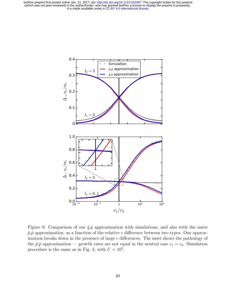
0

0.1

0.2

0.3

0.4

∆+ni/mi

l1 = 3

l2 = 3

Simulation

p,p approximation

q,q approximation

10−2 10−1 1 101 102

c1/c2

0.0

0.2

0.4

0.6

0.8

1.0

∆+ni/mi

l1 = 0. 1

l2 = 3

1

Figure 9: Comparison of our q,q approximation with simulations, and also with the naivep,p approximation, as a function of the relative c difference between two types. Our approx-imation breaks down in the presence of large c differences. The inset shows the pathology ofthe p,p approximation — growth rates are not equal in the neutral case c1 = c2. Simulationprocedure is the same as in Fig. 3, with U = 105.

40



http://dx.doi.org/10.1101/102087


Similarly to Eq. (29), the right hand side of Eq. (31) is small for both low and high665

nonfocal densities. Again, the worst case scenario occurs when li and L − li are of order 1,666

but Eq. (17) is still a good approximation in this case. Again, the approximation breaks667

down in the presence of a rare, strong competitor (Fig. 9).668

Appendix B: Total density in the Lotka-Volterra com-669

petition model670

Here we show that under the Lotka-Volterra model of competition, total density N does not671

in general remain constant over a selective sweep in a crowded population even if the types672

have the same equilibrium density (for a related discussion on the density- and frequency-673

dependence of selection in the Lotka-Volterra model, see (Smouse, 1976; Mallet, 2012)).674

We assume equal effects of crowding within types α11 = α22 = αintra and N = 1/αintra and

check whether it is then possible for dNdt

to be zero in the sweep (n1, n2 6= 0). Substituting

these conditions into Eq. (10), we obtain

dn1

dt= r1(α11 − α12)n1n2

dn2

dt= r2(α22 − α21)n1n2 (32)

Adding these together, dNdt

can only be zero if675

r1(αintra − α12) + r2(αintra − α21) = 0. (33)

To get some intuition for Eq. (33), suppose that a mutant arises with improved competitive676

ability but identical intrinsic growth rate and equilibrium density (r1 = r2 and α11 = α22).677

This could represent a mutation to an interference competition trait, for example (Gill,678

41



http://dx.doi.org/10.1101/102087


1974). Then, according the above condition, for N to remain constant over the sweep, the679

mutant must find the wildtype more tolerable than itself by exactly the same amount that680

the wildtype finds the mutant less tolerable than itself.681

Even if we persuaded ourselves that this balance of inter-type interactions is plausible682

in some circumstances, when multiple types are present the requirement for constant N683

becomes684 ∑ij

ri(αintra − αij)pipj = 0, (34)

which depends on frequency and thus cannot be satisfied in general for constant inter-type685

coefficients αij. Therefore, Lotka-Volterra selection will generally involve non-constant N .686

Appendix C: Density-dependence of b-selection687

In section “Density-regulating traits and the threat of strong selection” we argued that the688

density-dependent factor f(b,N) = 1−e−bN/T

N(T −N) is unchanged at the beginning and end689

points of an equilibrium to equilibrium sweep of a type with higher b. Here we estimate the690

magnitude of the deviation in f(b,N) during the sweep.691

For simplicity, we introduce the notation D = N/T and assume that D is small. We

can thus make the approximation 1 − e−bD ≈ bD and f(b,N) ≈ b(1 − D). We expect

this to be a conservative approximation based on the worst case scenario, because N is

most sensitive to an increase in b in this low-density linear regime. We first calculate the

value of f(b,N) at the halfway point in a sweep, where the halfway point is estimated with

simple linear averages for b and N . The sweep is driven by a b variant with b2 = b1(1 + ε),

and we denote the initial and final densities by D1 and D2 respectively, where we have

42



http://dx.doi.org/10.1101/102087


finitial = b1(1−D1) = d1 − 1 = ffinal = b2(1−D2). We obtain

fhalf = f(b1 + b2

2,N1 +N2

2) =

b1 + b2

2

(1− D1 +D2

2

)=

1

4(b1 + b2)(2−D1 −D2)

=1

4(2(d1 − 1) + b1(1−D2) + b2(1−D1)). (35)

Dividing by d1 − 1, the proportional deviation in f(N) at the midpoint of the sweep is

fhalf

d1 − 1=

1

4

(2 +

b1

b2

+b2

b1

)=

1

4

(2 +

1

1 + ε+ 1 + ε

)= 1 +

1

4(ε2 − ε3 + . . .), (36)

where we have used the Taylor expansion 11+ε

= 1− ε+ ε2 − ε3 + . . ..692

By contrast, for a δ sweep in Eq. (11), the density-dependent term N increases by a693

factor of 11−ε = 1 + ε + ε2 + . . .. Thus, the deviations in f(N) are an order of magnitude694

smaller than those shown in Fig. (6).695

43



http://dx.doi.org/10.1101/102087


density-dependent selection and the limits of relative fitness

Documents