DEPARTMENT OF AUTOMOBILE ENGINEERING

SCHOOL OF MECHANICAL ENGINEERING

STRENGTH OF MATERIALS

Details of Lecturer

Course Lecturer: Mr.K.Arun kumar (Asst. Professor)

COURSE GOALS

       This course has two specific goals:(i)  To introduce students to concepts of stresses and

strain; shearing force and bending; as well as torsion and deflection of different structural elements.

(ii) To develop theoretical and analytical skills relevant to the areas mentioned in (i) above.

COURSE OUTLINE

UNIT TITLE CONTENTS

I DEFORMATION OF SOLIDS

Introduction to Rigid and Deformable bodies – properties, Stresses - Tensile, Compressive and Shear, Deformation of simple and compound bars under axial load – Thermal stress – Elastic constants – Volumetric Strain, Strain energy and unit strain energy

II TORSION Introduction - Torsion of Solid and hollow circular bars – Shear stress distribution – Stepped shaft – Twist and torsion stiffness – Compound shafts – Springs – types - helical springs – shear stress and deflection in springs

III BEAMS Types : Beams , Supports and Loads – Shear force and Bending Moment – Cantilever, Simply supported and Overhanging beams – Stresses in beams – Theory of simple bending – Shear stresses in beams – Evaluation of ‘I’, ‘C’ & ‘T’ sections

COURSE OUTLINE

UNIT TITLE CONTENTS

IV DEFLECTION OF BEAMS

Introduction - Evaluation of beam deflection and slope: Macaulay Method and Moment-area Method

V ANALYSIS OF STRESSES IN

TWO DIMENSIONS

Biaxial state of stresses – Thin cylindrical and spherical shells – Deformation in thin cylindrical and spherical shells – Principal planes and stresses – Mohr’s circle for biaxial stresses – Maximum shear stress - Strain energy in bending and torsion

TEXT BOOKS•Bansal, R.K., A Text Book of Strength of Materials, Lakshmi Publications Pvt. Limited, New Delhi, 1996•Ferdinand P.Beer, and Rusell Johnston, E., Mechanics of Materials, SI Metric Edition, McGraw Hill, 1992

Course Objectives

  Upon successful completion of this course, students should be able to:

(i)  Understand and solve simple problems involving stresses and strain in two and three dimensions.

(ii) Understand the difference between statically determinate and indeterminate problems.

(iv) Analyze stresses in two dimensions and understand the concepts of principal stresses and the use of Mohr circles to solve two-dimensional stress problems.

COURSE OBJECTIVES CONTD.

(v) Draw shear force and bending moment diagrams of simple

beams and understand the relationships between loading

intensity, shearing force and bending moment.

(vi) Compute the bending stresses in beams with one or two

materials. (vii) Calculate the deflection of beams using the direct integration

and moment-area method.

Teaching Strategies

The course will be taught via Lectures. Lectures will also involve

the solution of tutorial questions. Tutorial questions are

designed to complement and enhance both the lectures and the

students appreciation of the subject.

Course work assignments will be reviewed with the students.

UNITS:

STRESS AND STRAIN

RELATIONS

UNIT I

DIRECT OR NORMAL STRESS

When a force is transmitted through a body, the body tends to change its shape or deform. The body is said to be strained.

Direct Stress = Applied Force (F) Cross Sectional Area (A)

Units: Usually N/m2 (Pa), N/mm2, MN/m2, GN/m2 or N/cm2

Note: 1 N/mm2 = 1 MN/m2 = 1 MPa

Direct Stress Contd.

Direct stress may be tensile or compressive and result from forces acting perpendicular to the plane of the cross-section

Tension

Compression

Tension and Compression

Direct or Normal Strain

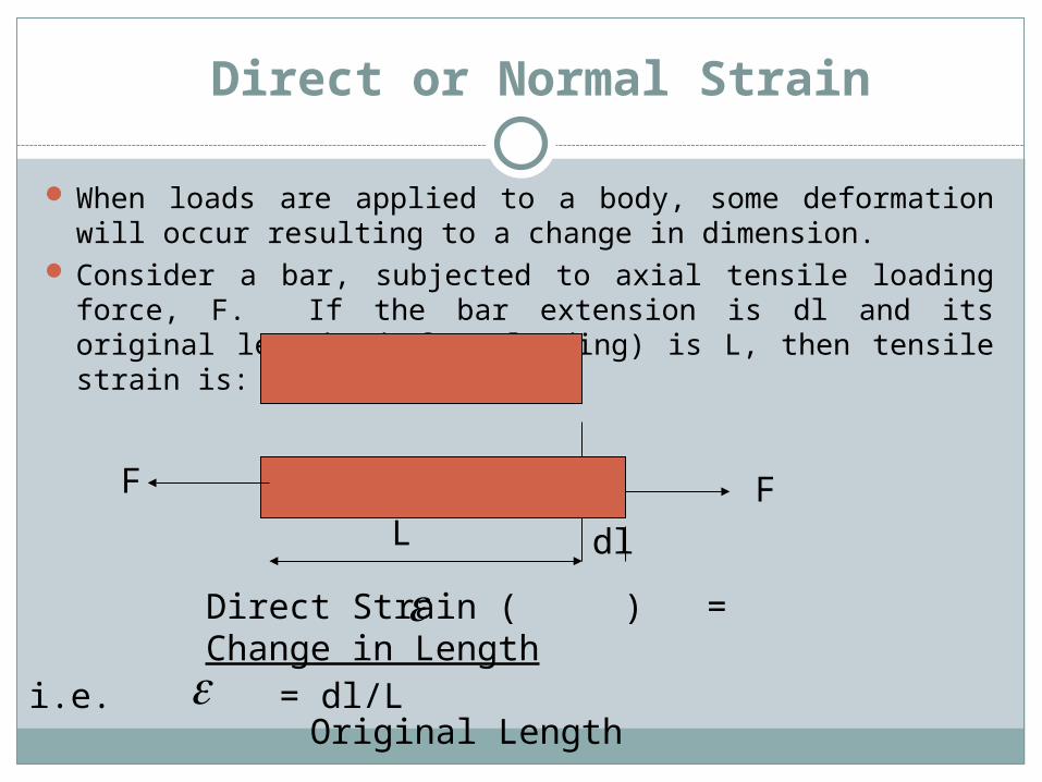
When loads are applied to a body, some deformation will occur resulting to a change in dimension.

Consider a bar, subjected to axial tensile loading force, F. If the bar extension is dl and its original length (before loading) is L, then tensile strain is:

dl

FF

L

Direct Strain ( ) = Change in Length Original Length

i.e. = dl/L

Direct or Normal Strain Contd.

As strain is a ratio of lengths, it is dimensionless. Similarly, for compression by amount, dl:

Compressive strain = - dl/LNote: Strain is positive for an increase in dimension

and negative for a reduction in dimension.

Shear Stress and Shear Strain

Shear stresses are produced by equal and opposite parallel forces not in line.

The forces tend to make one part of the material slide over the other part.

Shear stress is tangential to the area over which it acts.

Ultimate Strength

The strength of a material is a measure of the stress that it can take when in use. The ultimate strength is the measured stress at failure but this is not normally used for design because safety factors are required. The normal way to define a safety factor is : 

stressePermissibl

stressUltimate

loadedwhen stress

failureat stress = factorsafety

Strain

We must also define strain. In engineering this is not a measure of force but is a measure of the deformation produced by the influence of stress. For tensile and compressive loads:

Strain is dimensionless, i.e. it is not measured in metres, killogrammes etc.

 For shear loads the strain is defined as the angle This is measured in radians

strain = increase in length x

original length L

shear strain shear displacement x

width L

Shear stress and strain

Shear force

Shear Force

Area resisting shear Shear displacement (x)

Shear strain is angle L

Shear Stress and Shear Strain Contd.

P Q

S R

FD D’

A B

C C’

L

x

Shear strain is the distortion produced by shear stress on an element or rectangular block as above. The shear strain, (gamma) is given as:

= x/L = tan

Shear Stress and Shear Strain Concluded

For small ,

Shear strain then becomes the change in the right angle.

It is dimensionless and is measured in radians.

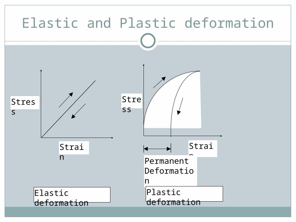
Elastic and Plastic deformation

Stress

Strain

Stress

Strain

Permanent Deformation

Elastic deformation Plastic deformation

Modulus of Elasticity

If the strain is "elastic" Hooke's law may be used to define

Young's modulus is also called the modulus of elasticity or stiffness and is a measure of how much strain occurs due to a given stress. Because strain is dimensionless Young's modulus has the units of stress or pressure

A

L

x

W =

Strain

Stress = E Modulus Youngs

How to calculate deflection if the proof stress is applied and then partially removed.

Yield

0.2% proof stress

Stress

Strain0.2%

Plastic

Failures

0.002 s/E

If a sample is loaded up to the 0.2% proof stress and then unloaded to a stress s the strain x = 0.2% + s/E where E is the Young’s modulus

Volumetric Strain

Hydrostatic stress refers to tensile or compressive stress in all dimensions within or external to a body.

Hydrostatic stress results in change in volume of the material.

Consider a cube with sides x, y, z. Let dx, dy, and dz represent increase in length in all directions.

i.e. new volume = (x + dx) (y + dy) (z + dz)

Volumetric Strain Contd.

Neglecting products of small quantities:New volume = x y z + z y dx + x z dy + x y dz Original volume = x y z = z y dx + x z dy + x y dzVolumetric strain, = z y dx + x z dy + x y dz

x y z = dx/x + dy/y + dz/z

V v

v

v x y z

Elasticity and Hooke’s Law

All solid materials deform when they are stressed, and as stress is increased, deformation also increases.

If a material returns to its original size and shape on removal of load causing deformation, it is said to be elastic.

If the stress is steadily increased, a point is reached when, after the removal of load, not all the induced strain is removed.

This is called the elastic limit.

Hooke’s Law

States that providing the limit of proportionality of a material is not exceeded, the stress is directly proportional to the strain produced.

If a graph of stress and strain is plotted as load is gradually applied, the first portion of the graph will be a straight line.

The slope of this line is the constant of proportionality called modulus of Elasticity, E or Young’s Modulus.

It is a measure of the stiffness of a material.

Hooke’s Law

Modulus of Elasticity, E = Directstress

Directstrain

Also: For Shear stress: Modulus of rigidity or shear modulus, G = Shearstress

Shearstrain

Also: Volumetric strain, is proportional to hydrostatic stress,

within the elastic range

i.e. : called bulk modulus.

v

/ v K

Stress-Strain Relations of Mild Steel

Equation For Extension

From the above equations:

EFA

dl L

FL

Adl

dlFL

AE

/

/

This equation for extension is very important

Extension For Bar of Varying Cross Section

F o r a b a r o f v a r y in g c r o s s s e c t io n :

P

A 1 A 2 A 3 P

L 1 L 2 L 3

d lF

E

L

A

L

A

L

A

LNM

OQP

1

1

2

2

3

3

Factor of Safety

The load which any member of a machine carries is called working load, and stress produced by this load is the working stress.

Obviously, the working stress must be less than the yield stress, tensile strength or the ultimate stress.

This working stress is also called the permissible stress or the allowable stress or the design stress.

Factor of Safety Contd.

Some reasons for factor of safety include the inexactness or inaccuracies in the estimation of stresses and the non-uniformity of some materials.

Factor of safety = Ultimateoryieldstress

Designorworkingstress

Note: Ultimate stress is used for materials e.g. concrete which do not have a well-defined yield point, or brittle materials which behave in a linear manner up to failure. Yield stress is used for other materials e.g. steel with well defined yield stress.

Results From a Tensile Test

(a) Modulus of Elasticity, EStress up to it of proportionality

Strain

lim

(b) Yield Stress or Proof Stress (See below)

(c) Percentage elongation = Increase in gauge length

Original gauge lengthx 100

(d ) P ercentage reduction in a rea = O riginal area area at fracture

O riginal areax

100

(e ) Tensile S trength = M axim um load

O riginal cross tional areasec

The percentage o f e longation and percentage reduction in a rea g ive an ind ica tion o f th e

ductility o f the m ateria l i.e . its ab ility to w ithstand stra in w ithou t fracture occurring .

Proof Stress

High carbon steels, cast iron and most of the non-ferrous alloys do not exhibit a well defined yield as is the case with mild steel.

For these materials, a limiting stress called proof stress is specified, corresponding to a non-proportional extension.

The non-proportional extension is a specified percentage of the original length e.g. 0.05, 0.10, 0.20 or 0.50%.

Determination of Proof Stress

PProof StressStress

The proof stress is obtained by drawing AP parallel to the initial slope of the stress/strain graph, the distance, OA being the strain corresponding to the required non-proportional extension e.g. for 0.05% proof stress, the strain is 0.0005.

A Strain

Thermal Strain

Most structural materials expand when heated,

in accordance to the law: T

where is linear strain and is the coefficient of linear expansion; T is the rise in temperature.

That is for a rod of Length, L;

if its temperature increased by t, the extension,

dl = L T.

Thermal Strain Contd.

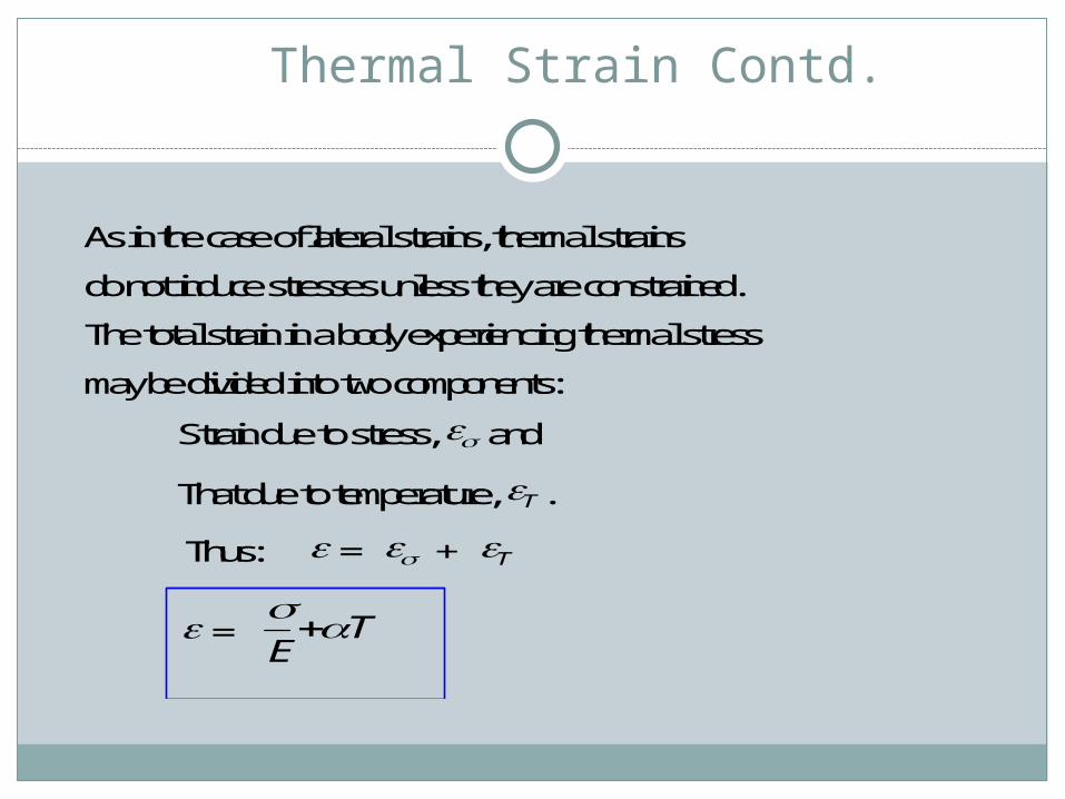
As in the case of lateral strains, thermal strains

do not induce stresses unless they are constrained.

The total strain in a body experiencing thermal stress

may be divided into two components:

Strain due to stress, and

That due to temperature, T.

Thus: = + T

= E

T

Principle of Superposition

It states that the effects of several actions taking place simultaneously can be reproduced exactly by adding the effect of each action separately.

The principle is general and has wide applications and holds true if:

(i) The structure is elastic (ii) The stress-strain relationship is linear (iii) The deformations are small.

General Stress-Strain Relationships

Relationship between Elastic Modulus (E) and Bulk Modulus, K

It has been shown that : v x y z

x x y z

x y z

x

y z

v x y z

v

v

v

EFor hydrostatic stress

i eE E

Similarly and are eachE

Volumetric strain

E

E

Bulk Modulus KVolumetric or hydrostatic stress

Volumetric strain

i e E K and KE

1

12 1 2

1 2

31 2

31 2

3 1 23 1 2

( )

,

. .

,

,

. .

Compound Bars

A compound bar is one comprising two or more parallel elements, of different materials,

which are fixed together at their end. The compound bar may be loaded in tension or

compression.

1 2

F F

2

Section through a typical compound bar consisting of a circular bar (1) surrounded by a

tube (2)

Temperature stresses in compound bars

1 1

2 2

L

(a) L1T

1

L2T

2 {b} FL

AE1 1

F 1 F

F 2 F

(c) FL

AE2 2

Temperature Stresses Contd.

Free expansions in bars (1) and (2) are L T and L T 1 2 respectively.

Due to end fixing force, F: the decrease in length of bar (1) is

FL

AE1 1

and the increase in length of (2) is FL

AE2 2

.

At Equilibrium:

L TFL

AEL T

FL

AE

i e FAE AE

T

i e AAE AE

EE AAT

T AEE

AE AE

T AEE

AE AE

11 1

22 2

1 1 2 21 2

1 12 2 1 1

1 2 1 21 2

11 2 2 1 2

1 1 2 2

21 2 1 1 2

1 1 2 2

1 1

LNM

OQP

. . [ ] ( )

. . ( )

( )

( )

Note: As a result of Force, F, bar (1) will be in compression while (2) will be in tension.

1 1

2 2

L

(a) L1T

1

L2T

2 {b} FL

AE1 1

F 1 F

F 2 F

(c) FL

AE2 2

Example

A steel tube having an external diameter of 36 mm and an internal diameter of 30 mm has a brass rod of 20 mm diameter inside it, the two materials being joined rigidly at their ends when the ambient temperature is 18 0C. Determine the stresses in the two materials: (a) when the temperature is raised to 68 0C (b) when a compressive load of 20 kN is applied at the increased temperature.

Example Contd.

For brass: Modulus of elasticity = 80 GN/m2; Coefficient of expansion = 17 x 10 -6 /0C

For steel: Modulus of elasticity = 210 GN/m2; Coefficient of expansion = 11 x 10 -6 /0C

Solution

3 0 B r a s s r o d 2 0 3 6

S t e e l t u b e

A r e a o f b r a s s r o d ( A b ) = x

m m2 0

43 1 4 1 6

22 .

A r e a o f s t e e l t u b e ( A s ) = x

m m( )

.3 6 3 0

43 1 1 0 2

2 22

A E x m x x N m x Ns s 3 1 1 0 2 1 0 2 1 0 1 0 0 6 5 3 1 4 2 1 06 2 9 2 8. / .

11 5 3 1 0 6 1 0 8

A Ex

s s

.

Solution Contd.

A E x m x x N m x Nb b 3 1 4 1 6 1 0 8 0 1 0 0 2 5 1 3 2 7 1 06 2 9 2 8. / .

13 9 7 8 8 7 3 6 1 0 8

A Ex

b b

.

T x xb s( ) ( ) 5 0 1 7 1 1 1 0 3 1 06 4

W i t h i n c r e a s e i n t e m p e r a t u r e , b r a s s w i l l b e i n c o m p r e s s i o n w h i l e

s t e e l w i l l b e i n t e n s i o n . T h i s i s b e c a u s e e x p a n d s m o r e t h a n s t e e l .

i e FA E A E

Ts s b b

b s. . [ ] ( )1 1

i . e . F [ 1 . 5 3 1 0 6 + 3 . 9 7 8 8 7 3 6 ] x 1 0 - 8 = 3 x 1 0 - 4

F = 5 4 4 4 . 7 1 N

Solution Concluded

S t r e s s i n s t e e l t u b e = 5 4 4 4 7 1

3 1 1 0 21 7 5 1 1 7 5 1

22 2.

.. / . / ( )

N

m mN m m M N m T e n s i o n

S t r e s s i n b r a s s r o d = 5 4 4 4 7 1

3 1 4 1 61 7 3 3 1 7 3 32

2 2.

.. / . / ( )

N

m mN m m M N m C o m p r e s s i o n

( b ) S t r e s s e s d u e t o c o m p r e s s i o n f o r c e , F ’ o f 2 0 k N

ss

s s b b

F E

E A E A

x N x x N m

xM N m C o m p r e s s i o n

' /

. .. / ( )

2 0 1 0 2 1 0 1 0

0 6 5 3 1 4 2 0 2 5 1 3 2 7 1 04 6 4 4

3 9 2

82

bb

s s b b

F E

E A E A

x N x x N m

xM N m C o m p r e s s i o n

' /

. .. / ( )

2 0 1 0 8 0 1 0

0 6 5 3 1 4 2 0 2 5 1 3 2 7 1 01 7 6 9

3 9 2

82

R e s u l t a n t s t r e s s i n s t e e l t u b e = - 4 6 . 4 4 + 1 7 . 5 1 = 2 8 . 9 3 M N / m 2 ( C o m p r e s s i o n )

R e s u l t a n t s t r e s s i n b r a s s r o d = - 1 7 . 6 9 - 1 7 . 3 3 = 3 5 . 0 2 M N / m 2 ( C o m p r e s s i o n )

Example

A composite bar, 0.6 m long comprises a steel bar 0.2 m long and 40 mm diameter which is fixed at one end to a copper bar having a length of 0.4 m.

Determine the necessary diameter of the copper bar in order that the extension of each material shall be the same when the composite bar is subjected to an axial load.

What will be the stresses in the steel and copper when the bar is subjected to an axial tensile loading of 30 kN? (For steel, E = 210 GN/m2; for copper, E = 110 GN/m2)

Solution

0.2 mm

0.4 mm

F 40 mm dia d F

Let the diameter of the copper bar be d mm

Specified condition: Extensions in the two bars are equal

dl dl

dl LE

LFL

AE

c s

Thus: F L

A E

F L

A Ec c

c c

s s

s s

Solution Concluded

A l s o : T o t a l f o r c e , F i s t r a n s m i t t e d b y b o t h c o p p e r a n d s t e e l

i . e . F c = F s = F

i eL

A E

L

A Ec

c c

s

s s

. .

S u b s t i t u t e v a l u e s g i v e n i n p r o b l e m :

0 4

4 1 1 0 1 0

0 2

4 0 0 4 0 2 1 0 1 02 2 9 2 2 9 2

.

/ /

.

/ . /

m

d m x N m

m

x x x N m

dx x

m d m m m22

22 2 1 0 0 0 4 0

1 1 00 0 7 8 1 6 7 8 1 6

.; . . .

T h u s f o r a l o a d i n g o f 3 0 k N

S t r e s s i n s t e e l , s

x N

x xM N m

3 0 1 0

4 0 0 4 0 1 02 3 8 7

3

2 62

/ .. /

S t r e s s i n c o p p e r , c

x N

x xM N m

3 0 1 0

4 0 0 7 8 1 6 1 09

3

2 62

/ ./

Elastic Strain Energy

If a material is strained by a gradually applied load, then work is done on the material by the applied load.

The work is stored in the material in the form of strain energy.

If the strain is within the elastic range of the material, this energy is not retained by the material upon the removal of load.

Elastic Strain Energy Contd.

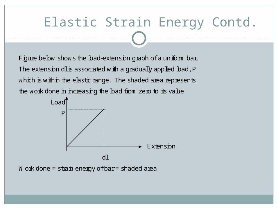
Figure below shows the load-extension graph of a uniform bar.

The extension dl is associated with a gradually applied load, P

which is within the elastic range. The shaded area represents

the work done in increasing the load from zero to its value

Load

P

Extension

dl

Work done = strain energy of bar = shaded area

Elastic Strain Energy Concluded

W = U = 1/2 P dl (1)

Stress, = P/A i.e P = A

Strain = Stress/E

i.e dl/L = /E , dl = (L)/E L= original length

Substituting for P and dl in Eqn (1) gives:

W = U = 1/2 A . ( L)/E = 2/2E x A L

A L is the volume of the bar.

i.e U = 2/2E x Volume

The units of strain energy are same as those of work i.e. Joules. Strain energy

per unit volume, 2/2E is known as resilience. The greatest amount of energy that can

stored in a material without permanent set occurring will be when is equal to the

elastic limit stress.

TORSION

UNIT 2

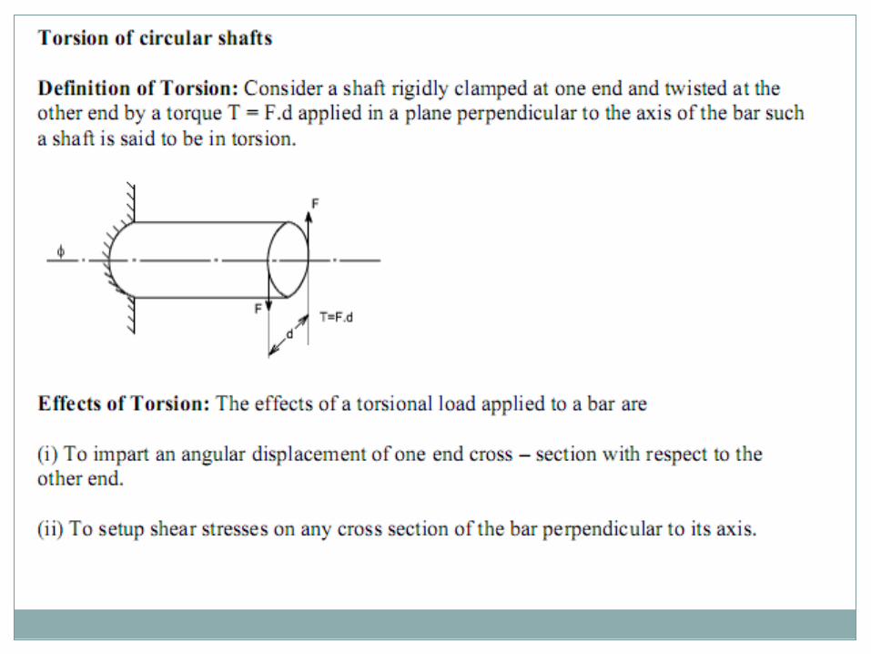
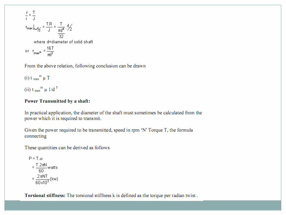
TORSION OF HOLLOW SHAFTS: From the torsion of solid shafts of circular x – section , it is seen that only the material atthe outer surface of the shaft can be stressed to the limit assigned as an allowable working stresses. All of the material within the shaft will work at a lower stress and is not being used to full capacity. Thus, in these cases where the weight reduction is important, it is advantageous to use hollow shafts. In discussing the torsion of hollow shafts the same assumptions will be made as in the case of a solid shaft. The general torsion equation as we have applied in the case of torsion of solid shaft will hold good

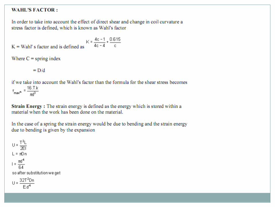
Derivation of the Formula : In order to derive a necessary formula which governs the behaviour of springs, consider a closed coiled spring subjected to an axial load W.

Let W = axial load D = mean coil diameter d = diameter of spring wire n = number of active coils C = spring index = D / d For circular wires l = length of spring wire G = modulus of rigidity x = deflection of spring q = Angle of twist when the spring is being subjected to an axial load to the wire of the spring gets be twisted like a shaft. If q is the total angle of twist along the wire and x is the deflection of spring under the action of load W along the axis of the coil, so that x = D / 2 . q again l = p D n [ consider ,one half turn of a close coiled helical spring ]

Assumptions: (1) The Bending & shear effects may be neglected (2) For the purpose of derivation of formula, the helix angle is considered to be so small that it may be neglected. Any one coil of a such a spring will be assumed to lie in a plane which is nearly ^r to the axis of the spring. This requires that adjoining coils be close together. With this limitation, a section taken perpendicular to the axis the spring rod becomes nearly vertical. Hence to maintain equilibrium of a segment of the spring, only a shearing force V = F and Torque T = F. r are required at any X – section. In the analysis of springs it is customary to assume that the shearing stresses caused by the direct shear force is uniformly distributed and is negligible so applying the torsion formula.

BEAMS

UNIT 3

Cantilever Beam

BENDING MOMENT

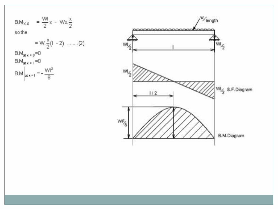
Basic Relationship Between The Rate of Loading, Shear Force and Bending Moment: The construction of the shear force diagram and bending moment diagrams is greatly simplified if the relationship among load, shear force and bending moment is established. Let us consider a simply supported beam AB carrying a uniformly distributed load w/length. Let us imagine to cut a short slice of length dx cut out from this loaded beam at distance ‘x' from the origin ‘0'.

The forces acting on the free body diagram of the detached portion of this loaded beam are the following • The shearing force F and F+ dF at the section x and x + dx respectively.

•The bending moment at the sections x and x + dx be M and M + dM respectively. • Force due to external loading, if ‘w' is the mean rate of loading per unit length then the total loading on this slice of length dx is w. dx, which is approximately acting through the centre ‘c'. If the loading is assumed to be uniformly distributed then it would pass exactly through the centre ‘c'. This small element must be in equilibrium under the action of these forces and couples. Now let us take the moments at the point ‘c'. Such that

A cantilever of length carries a concentrated load ‘W' at its free end.

Draw shear force and bending moment. Solution: At a section a distance x from free end consider the forces to the left, then F = -W (for all values of x) -ve sign means the shear force to the left of the x-section are in downward direction and therefore negative. Taking moments about the section gives (obviously to the left of the section) M = -Wx (-ve sign means that the moment on the left hand side of the portion is in the anticlockwise direction and is therefore taken as –ve according to the sign convention) so that the maximum bending moment occurs at the fixed end i.e. M = -W l From equilibrium consideration, the fixing moment applied at the fixed end is Wl and the reaction is W. the shear force and bending moment are shown as,

Simply supported beam subjected to a central load (i.e. load acting at the mid-way)

.For B.M diagram: If we just take the moments to the left of the cross-section,

A cantilever beam subjected to U.d.L, draw S.F and B.M diagram.

Here the cantilever beam is subjected to a uniformly distributed load whose intensity is given w / length. Consider any cross-section XX which is at a distance of x from the free end. If we just take the resultant of all the forces on the left of the X-section, then

Simply supported beam subjected to a uniformly distributed load U.D.L

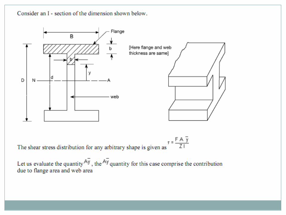
An I - section girder, 200mm wide by 300 mm depth flange and web of thickness is 20 mm is used as simply supported beam for a span of 7 m. The girder carries a distributed load of 5 KN /m and a concentrated load of 20 KN at mid-span. Determine the (i). The second moment of area of the cross-section of the girder (ii). The maximum stress set up.

Solution: The second moment of area of the cross-section can be determained as follows : For sections with symmetry about the neutral axis, use can be made of standard I value for a rectangle about an axis through centroid i.e. (bd 3 )/12. The section can thus be divided into convenient rectangles for each of which the neutral axis passes through the centroid. Example in the case enclosing the girder by a rectangle

DEFLECTION OF BEAMS

UNIT 4

Deflection of Beams The deformation of a beam is usually expressed in terms of its deflection from its original unloaded position. The deflection is measured from the original neutral surface of the beam to the neutral surface of the deformed beam. The configuration assumed by the deformed neutral surface is known as the elastic curve of the beam.

METHODS OF DETERMINING DEFLECTION OF BEAMS

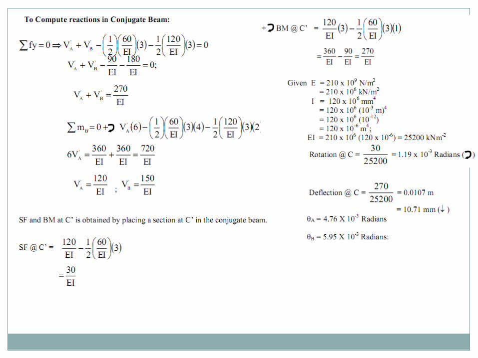
Double integration methodMoment area methodConjugate methodMacaulay's method

Example - Simply supported beam Consider a simply supported uniform section beam with a single load F at the centre. The beam will be deflect symmetrically about the centre line with 0 slope (dy/dx) at the centre line. It is convenient to select the origin at the centre line.

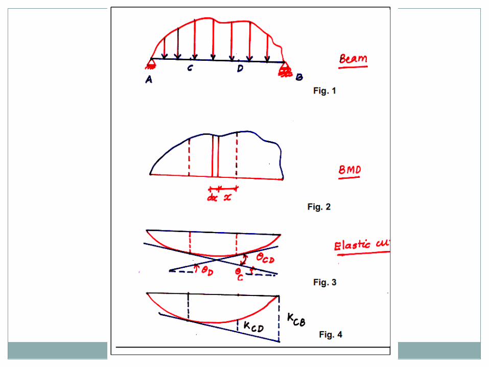
Moment Area Method This is a method of determining the change in slope or the deflection between two points on a beam. It is expressed as two theorems... Theorem 1 If A and B are two points on a beam the change in angle (radians) between the tangent at A and the tangent at B is equal to the area of the bending moment diagram between the points divided by the relevant value of EI (the flexural rigidity constant). Theorem 2 If A and B are two points on a beam the displacement of B relative to the tangent of the beam at A is equal to the moment of the area of the bending moment diagram between A and B about the ordinate through B divided by the relevant value of EI (the flexural rigidity constant).

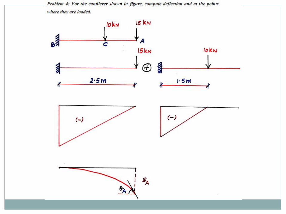
Examples ..Two simple examples are provide below to illustrate these theorems Example 1) Determine the deflection and slope of a cantilever as shown..

Moment Area Method This method is based on two theorems which are stated through an example. Consider a beam AB subjected to some arbitrary load as shown in Figure 1. Let the flexural rigidity of the beam be EI. Due to the load, there would be bending moment and BMD would be as shown in Figure 2. The deflected shape of the beam which is the elastic curve is shown in Figure 3. Let C and D be two points arbitrarily chosen on the beam. On the elastic curve, tangents are drawn at deflected positions of C and D. The angles made by these tangents with respect to the horizontal are marked as and . These angles are nothing but slopes. The change is the angle between these two tangents is demoted as . This change in the angel is equal to the area of the diagram between the two points C and D. This is the area of the shaded portion in figure 2.

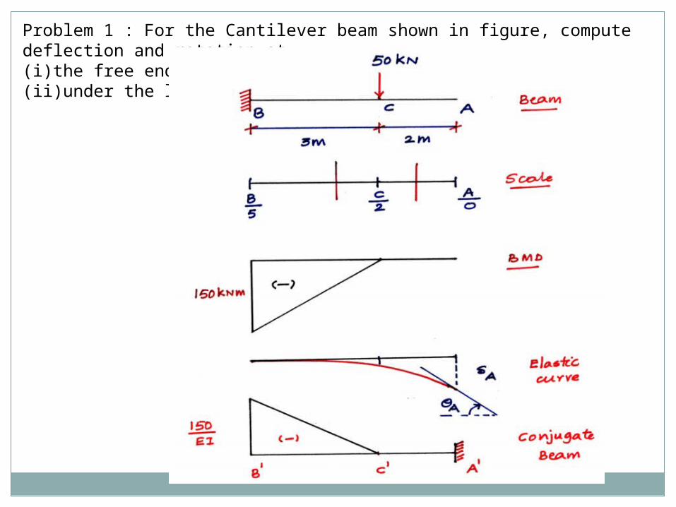
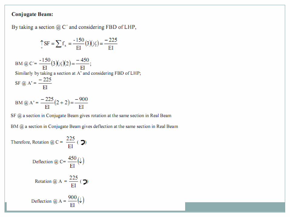
Problem 1 : For the Cantilever beam shown in figure, compute deflection and rotation at (i)the free end (ii)under the load

Macaulay's Methods If the loading conditions change along the span of beam, there is corresponding change in moment equation. This requires that a separate moment equation be written between each change of load point and that two integration be made for each such moment equation. Evaluation of the constants introduced by each integration can become very involved. Fortunately, these complications can be avoided by writing single moment equation in such a way that it becomes continuous for entire length of the beam in spite of the discontinuity of loading.

Note : In Macaulay's method some author's take the help of unit function approximation (i.e. Laplace transform) in order to illustrate this method, however both are essentially the same.

Procedure to solve the problems (i). After writing down the moment equation which is valid for all values of ‘x' i.e. containing pointed brackets, integrate the moment equation like an ordinary equation. (ii). While applying the B.C's keep in mind the necessary changes to be made regarding the pointed brackets. llustrative Examples : 1. A concentrated load of 300 N is applied to the simply supported beam as shown in Fig.Determine the equations of the elastic curve between each change of load point and the maximum deflection in the beam.

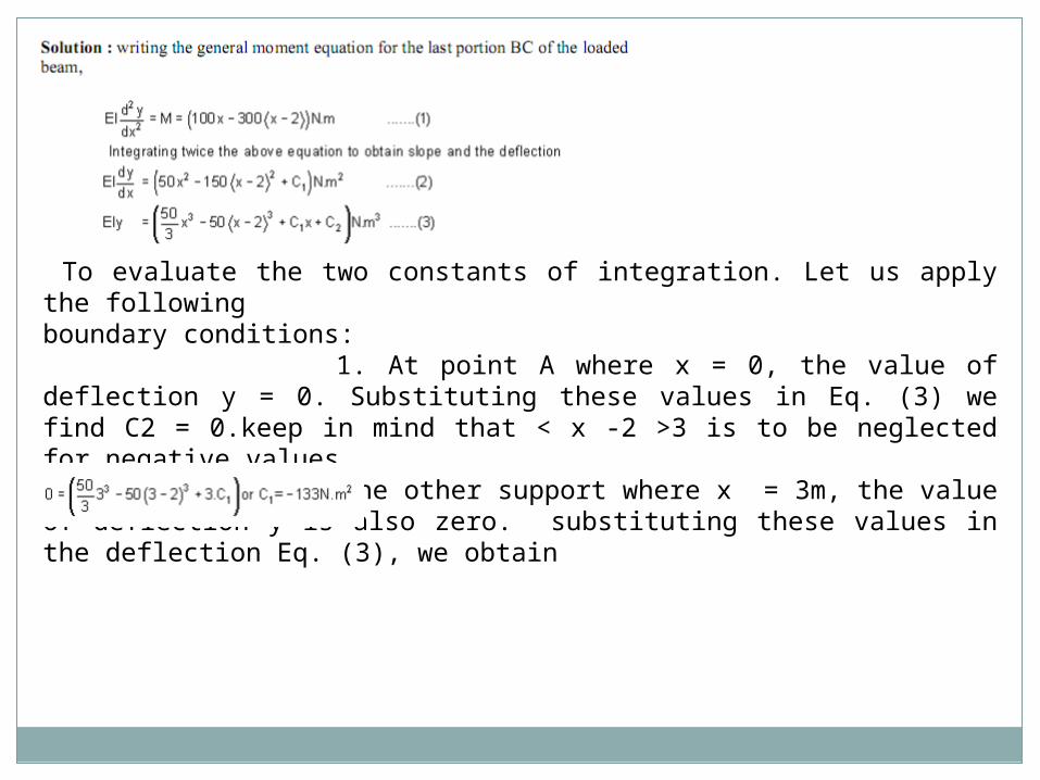
To evaluate the two constants of integration. Let us apply the following boundary conditions: 1. At point A where x = 0, the value of deflection y = 0. Substituting these values in Eq. (3) we find C2 = 0.keep in mind that < x -2 >3 is to be neglected for negative values. 2. At the other support where x = 3m, the value of deflection y is also zero. substituting these values in the deflection Eq. (3), we obtain

Continuing the solution, we assume that the maximum deflection will occur in the segment AB. Its location may be found by differentiating Eq. (5) with respect to x and setting the derivative to be equal to zero, or, what amounts to the same thing, setting the slope equation (4) equal to zero and solving for the point of zero slope.

50 x2– 133 = 0 or x = 1.63 m (It may be kept in mind that if the solution of the equation does not yield a value < 2 m then we have to try the other equations which are valid for segment BC)

Since this value of x is valid for segment AB, our assumption that the maximum deflection occurs in this region is correct. Hence, to determine the maximum deflection, we substitute x = 1.63 m in Eq (5), which yields

The negative value obtained indicates that the deflection y is downward from the x axis.quite usually only the magnitude of the deflection, without regard to sign, is desired; this is denoted by d, the use of y may be reserved to indicate a directed value of deflection.

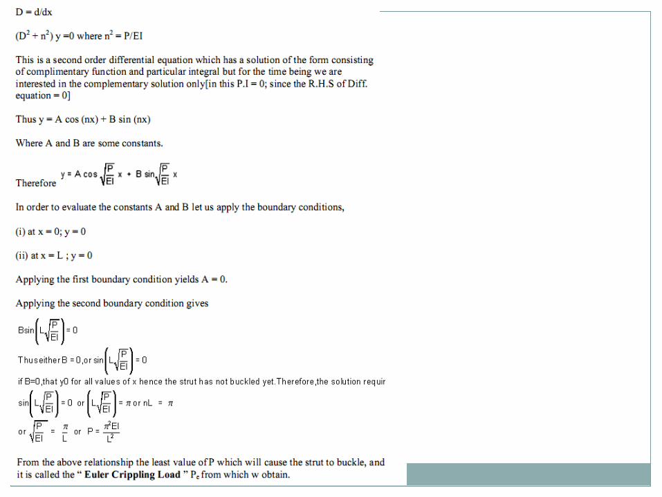
Limitations of Euler's Theory : In practice the ideal conditions are never [ i.e. the strut is initially straight and the end load being applied axially through centroid] reached. There is always some eccentricity and initial curvature present. These factors needs to be accommodated in the required formula's. It is realized that, due to the above mentioned imperfections the strut will suffer a deflection which increases with load and consequently a bending moment is introduced which causes failure before the Euler's load is reached. Infact failure is by stress rather than by buckling and the deviation from the Euler value is more marked as the slenderness-ratio l/k is reduced. For values of l/k < 120 approx, the error in applying the Euler theory is too great to allow of its use. The stress to cause buckling from the Euler formula for the pin ended strut is

ANALYSIS OF STRESSESS IN TWO DIMENSIONS

UNIT 5

4.1 DERIVATION OF GENERAL EQUATIONS

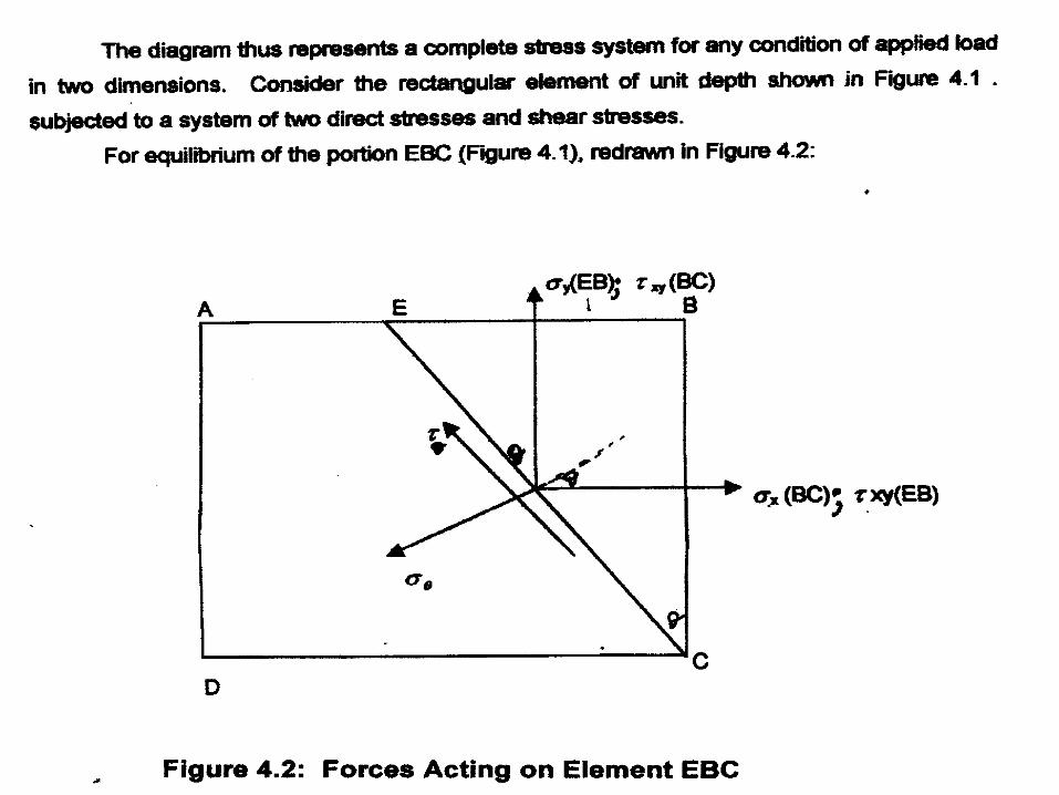
Resolving perpendicular to EC: x 1 x EC = x x BC x 1 x cos

+ y x EB x 1 x sin

+ xy x 1 x EB x cos

+ xy x 1 x BC x sin

Note that EB = EC sin and BC = EC cos

x EC = x x EC cos2 + y x EC sin

2

+ xy x EC x sin cos

+ xy x EC sin cos

= x cos2 + y sin

2 + 2 xy sin cos

Recall that : cos2 = (1 + cos 2)/2, sin 2 = (1 – cos 2)/2 and

sin 2 = 2 sin cos

= x/2 (1 + cos 2) + y/2 (1 - cos 2) + xy sin 2

x y x yxy2 2

2 2cos sin ………………… (4.1)

Resolving parallel to EC:

x 1 x EC = x x BC x 1 x sin + y x EB x 1 x cos

+ xy x 1 x EB x sin + xy x 1 x BC x cos

Derivation of General Equation Concluded

x E C = x x E C s i n c o s - y x E C s i n c o s +

x y x E C x s i n 2 - x y x E C c o s 2

= x s i n c o s - y s i n c o s + x y s i n 2 - x y c o s 2

R e c a l l t h a t s i n 2 = 2 s i n c o s a n d c o s 2 = c o s 2 - s i n 2

x yx y2

2 2s i n c o s … … … … … … … . ( 4 . 2 )

SPECIAL CASES OF PLANE STRESS

T h e g e n e r a l c a s e o f p l a n e s t r e s s r e d u c e s t o s i m p l e r s t a t e s o f s t r e s s u n d e r s p e c i a l c o n d i t i o n s : 4 . 1 . 1 U n i a x i a l S t r e s s : T h i s i s t h e s i t u a t i o n w h e r e a l l t h e s t r e s s e s a c t i n g o n t h e x y

e l e m e n t a r e z e r o e x c e p t f o r t h e n o r m a l s t r e s s x , t h e n t h e e l e m e n t i s i n u n i a x i a l

s t r e s s . T h e c o r r e s p o n d i n g t r a n s f o r m a t i o n e q u a t i o n s , o b t a i n e d b y s e t t i n g y a n d

x y e q u a l t o z e r o i n t h e E q u a t i o n s 4 . 1 a n d 4 . 2 a b o v e :

x x

21 2

22( c o s ) , s i n

Special Cases of Plane Stress Contd.

Maximum Shear Stress

Example

Solution

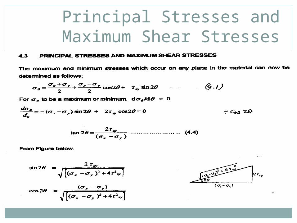
Principal Stresses and Maximum Shear Stresses

Principal Stresses and Maximum Shear Stresses

Contd.T h e s o l u t i o n o f e q u a t i o n 4 . 4 y i e l d s t w o v a l u e s o f 2 s e p a r a t e d b y 1 8 0 o , i . e . t w o v a l u e s

o f s e p a r a t e d b y 9 0 o . T h u s t h e t w o p r i n c i p a l s t r e s s e s o c c u r o n m u t u a l l y p e r p e n d i c u l a r

p l a n e s t e r m e d p r i n c i p a l p l a n e s ,

S u b s t i t u t i n g i n e q u a t i o n 4 . 1 :

x y x y

2 2

( )

( )

x y

x y x y

2 24 + x y

2

42 2

x y

x y x y( )

x y

2

( )

( )

x y

x y x y

2

2 22 4 +

2

4

2

2 2

x y

x y x y( )

x y

2

1

2

4

4

2 2

2 2

( )

( )

x y x y

x y x y

Shear Stresses at Principal Planes are Zero

1 o r 2 =

x yx y x y

2

1

242 2) … … . . ( 4 . 5 )

T h e s e a r e t e r m e d t h e p r i n c i p a l s t r e s s e s o f t h e s y s t e m . B y s u b s t i t u t i o n f o r

f r o m e q u a t i o n 4 . 4 , i n t o t h e s h e a r s t r e s s e x p r e s s i o n ( e q u a t i o n 4 . 2 ) :

x yx y2

2 2s i n c o s … … … … … … … . ( 4 . 2 )

x y

2

2

42 2

x y

x y x y( ) - x y

( )

( )

x y

x y x y

2 24

x y x y

x y x y

( )

( )

2 24 -

x y x y

x y x y

( )

( )

2 24 = 0

Principal Planes and Stresses Contd.

Thus at principal planes, = 0. Shear stresses do not occur at the principal planes. The complex stress system of Figure 4.1 can now be reduced to the equivalent system

of principal stresses shown in Figure 4.2 below.

Figure 4.3: Principal planes and stresses

Equation For Maximum Shear Stress

From equation 4.3, the maximum shear stress present in the system is given by:

max ( )1

2x y =1

242 2 x y xy )

and this occurs on planes at 45o to the principal planes. Note: This result could have been obtained using a similar procedure to that used for

determining the principal stresses, i.e. by differentiating expression 4.2, equating to

zero and substituting the resulting expression for

4.4 PRINCIPAL PLANE INCLINATION IN TERMS OF THE ASSOCIATED

PRINCIPAL STRESS It has been stated in the previous section that expression (4.4), namely

tan( )

22 xy

x y

yields two values of , i.e. the inclination of the two principal planes on which the

principal stresses 1 or 2. It is uncertain, however, which stress acts on which

plane unless eqn. (4.1 ) is used, substituting one value of obtained from eqn. (4.4)

and observing which one of the two principal stresses is obtained. The following

alternative solution is therefore to be preferred.

PRINCIPAL PLANE INCLINATION CONTD.

Consider once again the equilibrium of a triangular block of material of unit depth (Fig. 4.3); this time EC is a principal plane on which a principal stress acts,

and the shear stress is zero (from the property of principal planes).

PRINCIPAL PLANE INCLINATION CONTD.

Resolving forces horizontally,

(,x x BC x 1) + ( xy x EB x 1) = ( p x EC x l) cos

x EC cos + xy x EC sin = p x EC cos

x + xy tan = p

tan

p x

xy

… (4.7)

E

PRINCIPAL PLANE INCLINATION CONTD.

Thus we have an equation for the inclination of the principal planes in terms of the principal stress. If, therefore, the principal stresses are determined and substituted in the above equation, each will give the corresponding angle of the plane on which it acts and there can then be no confusion.

PRINCIPAL PLANE INCLINATION CONTD.

The above formula has been derived with two tensile direct stresses and a shear stress system, as shown in the figure; should any of these be reversed in action, then the appropriate minus sign must be inserted in the equation.

Graphical Solution Using the Mohr’s Stress Circle

4.5. GRAPHICAL SOLUTION-MOHR'S STRESS CIRCLE Consider the complex stress system of Figure below. As stated previously this represents a complete stress system for any condition of applied load in two dimensions. In order to find graphically the direct stress p and shear stress on any plane inclined at to the plane on which x acts, proceed as follows:

(1) Label the block ABCD.

(2) Set up axes for direct stress (as abscissa) and shear stress (as ordinate)

(3) Plot the stresses acting on two adjacent faces, e.g. AB and BC, using the following

sign conventions:

Mohr’s Circle Contd.

Direct stresses: tensile, positive; compressive, negative;

Shear stresses: tending to turn block clockwise, positive; tending to turn block

counterclockwise, negative.This gives two points on the graph which may then

be labeled AB and BC respectively to denote stresses on these planes

Mohr’s Circle Contd.

Fig. 4.5 Mohr's stress circle.

(4) Join AB and BC.

(5) The point P where this line cuts the a axis is then the centre of Mohr's circle, and

the

line is the diameter; therefore the circle can now be drawn. Every point on the

circumference of the circle then represents a state of stress on some plane

through C.

y

xy

xy

x

A B

CD

Mohr's stress circle.

 

Proof

C o n s i d e r a n y p o i n t Q o n t h e c i r c u m f e r e n c e o f t h e c i r c l e , s u c h t h a t P Q m a k e s a n a n g l e 2 w i t h B C , a n d d r o p a p e r p e n d i c u l a r f r o m Q t o m e e t t h e a a x i s a t N .

C o o r d i n a t e s o f Q :

O N O P P N Rx y 1

22( ) c o s ( )

1

22 2( ) c o s c o s s i n s i n x y R R

R a n d Rx y x yc o s ( ) s i n 1

2

O N x y x y x y 1

2

1

22 2( ) ( ) c o s s i n

Proof Contd.

On inspection this is seen to be eqn. (4.1) for the direct stress on the plane inclined at to BC in the figure for the two-dimensional complex system.

Similarly,

QN sin ( 2 - )

= R sin 2 cos - R cos 2 sin

1

22 2( )sin cos x y xy

Again, on inspection this is seen to be eqn. (4.2) for the shear stress on the plane inclined at to BC.

Note

Thus the coordinates of Q are the normal and shear stresses on a plane

inclined at to BC in the original stress system.

N.B. - Single angle BCPQ is 2 on Mohr's circle and not , it is evident that angles are doubled on Mohr's circle. This is the only difference, however, as they are

measured in the same direction and from the same plane in both figures (in this case

counterclockwise from

~BC).

Further Notes on Mohr’s Circle

F u r th e r p o in t s t o n o te a r e :

( 1 ) T h e d ir e c t s t r e s s is a m a x im u m w h e n Q is a t M , i . e . O M is t h e le n g th r e p r e s e n t in g

t h e m a x im u m p r in c ip a l s t r e s s 1 a n d 2 1 g iv e s t h e a n g le o f t h e p la n e 1 f r o m

B C . S im i la r ly , O L is t h e o th e r p r in c ip a l s t r e s s .

( 2 ) T h e m a x im u m s h e a r s t r e s s is g iv e n b y t h e h ig h e s t p o in t o n t h e c ir c le a n d is

r e p r e s e n te d b y t h e r a d iu s o f t h e c ir c le . T h is f o l lo w s s in c e s h e a r s t r e s s e s a n d

c o m p le m e n ta r y s h e a r s t r e s s e s h a v e t h e s a m e v a lu e ; t h e r e fo r e t h e c e n t r e o f t h e

c ir c le w i l l a lw a y s l ie o n t h e 1 a x is m id w a y b e tw e e n x ya n d .

( 3 ) F r o m th e a b o v e p o in t t h e d ir e c t s t r e s s o n t h e p la n e o f m a x im u m s h e a r m u s t b e

m id w a y b e tw e e n x ya n d .

Further Notes on Mohr Circle Contd.

(4) The shear stress on the principal planes is zero.

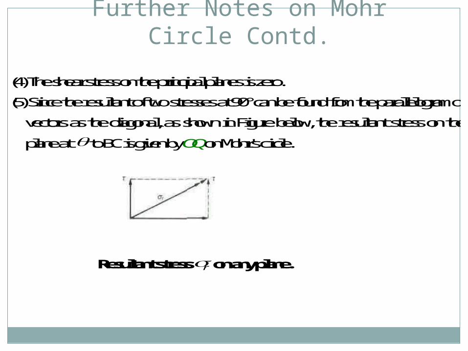
(5) Since the resultant of two stresses at 90° can be found from the parallelogram of

vectors as the diagonal, as shown in Figure below, the resultant stress on the

plane at to BC is given by OQ on Mohr's circle.

Resultant stress r on any plane.

Preference of Mohr Circle

The graphical method of solution of complex stress problems using Mohr's circle is a very powerful technique since all the information relating to any plane within the stressed element is contained in the single construction.

It thus provides a convenient and rapid means of solution which is less prone to arithmetical errors and is highly recommended.