department of economics & public policy working paper series
TRANSCRIPT

Department of Economics & Public Policy
Working Paper Series
WP 2014-04 September 2014
There Will Be Blood: Crime Rates in Shale-Rich
U.S. Counties
Alexander James
University of Alaska Anchorage
Department of Economics & Public Policy
Brock Smith
University of Oxford
Department of Economics
Center for Analysis of Resource Rich Economies
UAA DEPARTMENT OF ECONOMICS & PUBLIC POLICY
3211 Providence Drive
Rasmuson Hall 302
Anchorage, AK 99508
http://www.cbpp.uaa.alaska.edu/econ/econhome.aspx

There Will Be Blood: Crime Rates in Shale-Rich U.S.
Counties
Alexander James∗ Brock Smith†
September 25, 2014
Preliminary and Incomplete
Abstract
Over the past decade, the production of shale oil and gas significantly increased in the
United States. This paper uniquely examines how this energy boom has affected regional
crime rates throughout the United States. There is evidence that, as a result of the
ongoing shale-energy boom, shale-rich counties experienced faster growth in rates of
both property and violent crimes including rape, assault, murder, robbery, burglary,
larceny and grand-theft auto. These results are particularly robust for rates of assault,
and less so for other types of crimes. Examining the migratory behavior of convicted sex
offenders indicates that boomtowns disproportionately attract convicted felons. Policy
makers should anticipate these effects and invest in public infrastructure accordingly.
Keywords: Natural Resources; Hydraulic Fracturing; Crime; Resource Curse.
JEL Classification: Q3; R11; K42;
∗Center for the Analysis of Resource Rich Economies, Department of Economics, University of Oxford,Oxford, UK. [email protected]†Center for the Analysis of Resource Rich Economies, Department of Economics, University of Oxford,
Oxford, UK. [email protected]
1

1 Introduction
In the early 2000’s, the exploration and production of oil and gas sharply increased in the
United States. While some of the increased production was arguably due to high oil and
gas prices, it is largely due to advancements in horizontal drilling and hydraulic fracturing
technology that have made the extraction of shale gas and tight oil deposits economically
feasible. From 2000 to 2011, U.S. tight oil production increased from 94 to 507 million barrels
of oil, a 440% increase. Production of shale gas has followed a similar trend. From 2000 to
2011, production of shale gas increased from .30 to 7.94 trillion cubic feet, a 2,500% increase
(U.S. Energy Information Administration).
The direct economic effects of resource booms and the shale boom in particular have been
studied in the existing literature (see for example Black, McKinnish and Sanders, 2005; Weber,
2012; Alcott and Keniston, 2014). Generally, this literature finds that resource booms attract
labor, decrease unemployment rates and inflate local wages. However, much less attention
has been given to the economic and social externalities associated with resource booms. This
paper considers one such externality: crime.
This is a timely question to consider as recent publications in popular media outlets have
raised concerns that regional resource booms in places like North Dakota and Montana have
fueled epidemics of crime. In a New York Times article titled “An Oil Town Where Men are
Many and Women Are Hounded” John Eligon writes:
Jessica Brightbill, a single 24-year old who moved here [Williston, North Dakota]
from Grand Rapids, Mich., a year and a half ago, said she was walking to work at
3:30 in the afternoon when a car with two men suddenly pulled up behind her. One
hopped out and grabbed her by her arms and began dragging her. She let her body
go limp so she would be harder to drag. Eventually, a man in a truck pulled up and
began yelling at the men and she got away, she said. The episode left her rattled.
2
Such news stories are not rare. Writing for CNN Money, Blake Ellis describes the apparent
influx in criminal activity in Williston, North Dakota. He writes that “In a single month this
summer [2011], the [police] department received 1,000 calls—compared to the 4,000 calls it
received in the three-year period between 2007 and 2009.” While the majority of such articles
are written about the experience of North Dakota, similar articles have been written about
current boom towns in, for example, Montana (Healy, 2013), Pennsylvania (Levy, 2014) and
New Mexico (Clausing, 2014). There is a lack of consensus among policy makers though, that
energy booms attract or produce criminal activity. Responding to such concerns, Brad Gill, the
executive director of the Independent Oil and Gas Association of New York says “We’ve found
that the anti-natural gas folks will say just about anything to further their cause.” He goes
on to say that “We think that local governments are well equipped to deal with the benefits
and challenges that will arise out of increased natural gas development” (Engquist, 2013).
Similarly, while the North Dakota State Attorney General, Wayne Stenehjem, acknowledges
that crime has recently increased in North Dakota, he argues that there has been a proportional
increase in population such that crime rates have not changed (Michale, 2011).
Comprehensive and systematic studies documenting the relationship between a booming
resource sector and criminal activity are surprisingly scant. To the best of our knowledge,
the existing relevant literature is limited to case studies or regional examinations. There is
little unconditional evidence that resource booms led to higher rates of crime in North Dakota
(Putz et al., 2011)1 and Louisiana (Luthra, 2006), though, some evidence that the recent
gas boom has created crime in Sublette, Wyoming (Ecosystem Research Group, 2009). A
report by the Pennsylvania State University Justice Center for Research finds no evidence
that the recent increase in shale gas extraction in Pennsylvania has lead to increased crime
rates. Though, the authors of this study note that “...it is difficult to detect strong trends
within such a short time period [e.g., 2006-2010] and any observed changes may be due to1The report by Putz et al. describes crime rates in so-called “oil” counties in North Dakota from 1980 to
2005. Though, as can be seen in Figure 3, the oil boom in the Bakken started post 2005.
3
natural variation” (Kowalski and Zajac, 2012). Earlier research examining the criminal impact
of the oil price boom of the late 1970’s offers a mixed bag of evidence as well. Brookshire
and D’Arge (1980) examine how the booming resource industry in Rock Springs Wyoming in
the early 1970’s affected the quality of ecosystem services (hunting and related recreational
activities) and the level of criminal activity. Constraining the control group of cities to mini-
mize unobserved heterogeneity, they find little to no evidence that the resource boom elevated
total crime rates in Rock Springs. Freudenburg and Jones (1991) offer a nice review of some
of this earlier literature. They conclude that while existing case studies largely support the
idea that population growth leads to a more than proportional increase in crime, county-level
studies offer inconclusive evidence. Wilkinson et al. (1984), for example, found no signifi-
cant effect of population growth on violent crime rates in 197 non-metropolitan counties in
Arizona, Colorado, Utah, Wyoming, New Mexico and Montana. They did however find that
energy development projects significantly affected violent crime rates. Freudenburg and Jones
conclude by saying that “As is almost always the case, further research would be desirable,
although the feasibility of some of the desired research may remain quite low until the next
time a dramatic surge in commodity prices leads to the creation of new boomtowns.”
Using data from all U.S. counties across 12 years (2000 to 2011) this paper uniquely
examines how the recent shale-energy boom has affected regional crime rates. We find some
evidence that shale-rich U.S. counties experienced more rapid growth in rates of forcible rape,
aggravated assault, robbery, larceny and murder. With the exception of assault, these results
are only moderately robust. For assaults, we find statistically and economically significant
results across a variety of model specifications. Examining the migratory behavior of convicted
sex offenders indicates that boomtowns heterogeneously attract labor of a criminal type. While
shale-rich North Dakota counties have a large and disproportionate number of sex offenders
living in them, the majority of these offenders were registered offenders prior to moving to
North Dakota. This paper offers policy implications for optimal resource management in the
4

U.S. Local policy makers should anticipate a surge in crime, especially violent crime, at the
beginning of a resource boom. To the extent that crime may be averted through adaptation
and learning, such as locking ones doors and walking in pairs late at night, an information
campaign warning the public of elevated levels of risk may be a fruitful crime-fighting strategy.
One speculative interpretation of the results is that a resource boom—via induced criminal
behavior and subsequent heterogeneous labor migration—may facilitate a drain of human and
physical capital and could propagate a long-term resource curse.
2 Theoretical Motivation
There is of course a large economic and sociological literature that examines the causes of
both violent and property crimes. The seminal work of Gary Becker (1968) treats criminals as
rational economic agents that weigh the benefit of committing a crime against the expected
cost—the product of the probability of being caught and the associated punishment. It follows
that increasing the probability of being caught and increasing the resulting punishment may
effectively reduce crime rates. The corresponding empirical literature largely supports this
theory. For example, there is evidence that increasing the number of police officers per person
decreases crime rates (Marvell and Moody, 1996; Levitt 2004; Di Tella and Schargrodsky,
2004). This provides a clue as to why boom towns may experience elevated levels of criminal
activity. A booming resource sector inflates local wages and is likely to attract labor to both
the resource and the non-traded (service) industries from other economies. In the absence of
a proportional increase in police officers, this reduces the number of police per capita and thus
increases the probably of getting away with a crime. According to this theory, there need not
be anything peculiar or especially criminal about the migrants that move to a boom town, a
sudden increase in population alone is enough to fuel illegal activity.
It is also possible that the types of people that are attracted to boom towns may be
5

particularly prone to illegal behavior. Oil and gas drilling jobs are physically demanding and
are especially attractive to young men. Indeed, while 20-29 year-olds accounted for 35% of the
crimes in 2011, they represented only 14% of the U.S. population. Similarly, while roughly half
of the population is female, males accounted for 74% of the crimes committed in the U.S. in
2011. Table 1 describes some of this data in more detail.2 Males account for a large majority
of all types of crimes with the exception of Larceny-theft, for which they have only a slight
majority (56%). Note that for violent crimes including murder, forcible rape and robbery,
males account for close to or above 90% of all crimes. While roughly equal proportions of
the U.S. population was aged 20-29 and 50-59 in 2011, many more crimes were committed by
the younger group. For example, while less than 6% of murders were committed by people
aged 50-59, 43% of murders were committed by those aged 20-29. Similar relationships hold
for other types of crime as well, including rape, assault, robbery, burglary and theft. Illegal
activity that results from the demographic shift in boom towns may be aggravated by the
sudden income gains associated with resource booms as young and single men suddenly have
the financial means to use and abuse illicit substances and alcohol. Such concerns can be
further compounded by the unusual work schedules that often exist in the energy industry,
e.g., 14 days on and 7 long and boring days off (Carrington, Hogg and McIntosh, 2011).
Beyond criminal activity resulting directly from the demographic distribution of boom
towns, labor shortages, high wages and low levels of unemployment may heterogeneously at-
tract individuals that otherwise face barriers to enter into the labor market, e.g., those that
are currently unemployed or underemployed and looking for work. Among a host of factors
that determine labor market success rates, a history of drug use and a recorded criminal con-
viction significantly reduce an individual’s ability to find employment. In a controlled field
experiment, Pager (2003) finds that white convicted felons receive callbacks from a controlled2Crime data was collected from the Federal Bureau of Investigations 2011 Uniform Crime Statistics and is
available at www.fbi.gov/stats-services/crimestats. Population and demographic data were collected from theCensus Bureau, Population Estimates and can be found at www.census.gov.
6
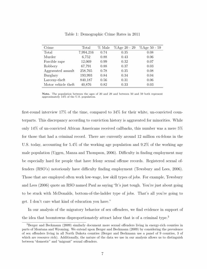
Table 1: Demographic Crime Rates in 2011
Crime Total % Male %Age 20 - 29 %Age 50 - 59Total 7,994,216 0.74 0.35 0.08Murder 6,752 0.88 0.43 0.06Forcible rape 12,069 0.99 0.32 0.07Robbery 67,791 0.88 0.37 0.03Aggravated assault 258,765 0.78 0.35 0.08Burglary 193,993 0.84 0.34 0.04Larceny-theft 840,187 0.56 0.31 0.06Motor vehicle theft 40,876 0.82 0.33 0.03
Note. The population between the ages of 20 and 29 and between 50 and 59 both representapproximately 14% of the U.S. population.
first-round interview 17% of the time, compared to 34% for their white, un-convicted coun-
terparts. This discrepancy according to conviction history is aggravated for minorities. While
only 14% of un-convicted African Americans received callbacks, this number was a mere 5%
for those that had a criminal record. There are currently around 12 million ex-felons in the
U.S. today, accounting for 5.4% of the working age population and 9.2% of the working age
male population (Uggen, Manza and Thompson, 2006). Difficulty in finding employment may
be especially hard for people that have felony sexual offense records. Registered sexual of-
fenders (RSO’s) notoriously have difficulty finding employment (Tewsbury and Lees, 2006).
Those that are employed often work low-wage, low skill types of jobs. For example, Tewsbury
and Lees (2006) quote an RSO named Paul as saying “It’s just tough. You’re just about going
to be stuck with McDonalds, bottom-of-the-ladder type of jobs. That’s all you’re going to
get. I don’t care what kind of education you have.”
In our analysis of the migratory behavior of sex offenders, we find evidence in support of
the idea that boomtowns disproportionately attract labor that is of a criminal type.3
3Berger and Beckmann (2009) similarly document more sexual offenders living in energy-rich counties inparts of Montana and Wyoming. We extend upon Berger and Beckmann (2009) by considering the prevalenceof sex offenders living in all North Dakota counties (Berger and Beckmann use a panel of 9 counties, 3 ofwhich are resource rich). Additionally, the nature of the data we use in our analysis allows us to distinguishbetween “domestic” and “migrant” sexual offenders.
7

Referencing again the seminal work of Gary Becker (1968) and Ehrlich (1973), unequal
growth in income and wealth may increase the expected gains from participating in a property
crime, at least for the so-called “have-nots”. And crimes resulting from observed income
inequality are not isolated to crimes against property either. According to strain theory, an
individual may be more likely to commit a violent crime when they feel economically or socially
alienated from a majority group (Merton, 1938). There is empirical evidence in favor of the
idea that economic inequality generates violent criminal activity. For example, in a study of
urban U.S. counties, Kelly (2000) finds that “for violent crime the impact of inequality is large,
even after controlling for the effects of poverty, race, and family composition.” The current
U.S. shale boom has generated high wages for people working in a variety of industries. In
North Dakota, for example, it is not uncommon for oil companies to pay workers $100,000
per year and truck drivers $80,000 per year. Fast-food restaurants there have experienced
labor shortages, forcing them to raise wages up to $15.00 per hour (Ellis, 2011). 4 For some
property owners though, oil and gas lease payments have played the most critical role in
generating additional income. In a 2011 New York Times article titled “A Great Divide Over
Oil Riches”, A. G. Sulzberger writes that “No other county [than Mountrail] in the state [of
North Dakota] has had a bigger jump in the number of households earning more than $100,000,
which spiked to 21 percent from 6 percent during the last decade...But much like the crude
below, the benefits have spread unevenly, often as a result of decisions made long ago...As
with any major boom—from real estate to tech stocks to natural resources—the sudden split
between the winners and the witnesses has been painful. But this is happening in a small
town, where proximity and familiarity make a sudden reordering all the more difficult.” He
goes on to discusses the experience of Lenin Dibble, a retired farmer living in a mobile home
that receives monthly royalty checks for as much as $80,000, per month. In describing the4In other parts of the country, fast-food workers earn an average wage of $9.00 per hour (Greenhouse, 2013)
and the average wage per job in the U.S. was just shy of $50,000 in 2012 (according to data collected from theBureau of Economic Analysis).
8
experience of Mr. Dibble, Sulzberger writes “What he and the others in town notice more
than the new-found money are the problems: locking the door to his house, taking the keys
out of his car and seeing a quiet community where everyone knew everyone overrun by the
bustle of strangers.”
Finally, an established sociological literature has argued that so-called “social disorganiza-
tion” contributes to regional crime trends. Unlike theories that concentrate on the types of
people that commit crimes, this literature focuses on the types of places that attract, nurture
or maintain criminal activity (Shaw and McKay, 1969; Sampson and Groves, 1989; Krubin
and Weitzer, 2003). According to Krubin and Weitzer, “Social disorganization refers to the in-
ability of a community to realize common goals and solve chronic problems. According to the
theory, poverty, residential mobility, ethnic heterogeneity, and weak social networks decrease a
neighborhood’s capacity to control the behavior of the people in public, and hence increase the
likelihood of crime.” Residential mobility may play a key role in explaining criminal activity
in boom towns as such events are typically characterized by a sudden inflow (and possibly
an outflow) of migrants. A loss of social cohesion and control offers would-be criminals two
advantages. First, it reduces the social cost of acting in socially undesirable ways and second,
it reduces the risk of getting caught as people don’t know each others’ names and neighbors
are less likely to keep a watchful eye on the neighborhood. As Freudenburg (1986) puts it
“When more of the faces in town are strange...a lawbreaker probably will find it easier to
escape detection and capture. He becomes a ‘white male, about 5 feet, 10 inches tall, between
the ages of 16 and 19,’ instead of ‘Ruth Johnson’s nephew, Frank.” ’
9
3 Data
3.1 Crime Data
The Federal Bureau of Investigations (FBI) provides county-level crime statistics as part of the
Uniform Crime Reporting (UCR) program.5 The Unified Crime Reports collect information on
reported crimes, not just those for which there was a conviction. The crimes considered in this
paper are those that the FBI refers to as “Part 1” crimes. These crimes are listed below along
with their definitions, taken directly from the 2009 FBI Uniform Crime Reporting Handbook.6
Criminal homicide—a.) Murder and non-negligent manslaughter: the willful (non-negligent)
killing of one human being by another. Deaths caused by negligence, attempts to kill,
assaults to kill, suicides, and accidental deaths are excluded. The program classifies
justifiable homicides separately and limits the definition to: (1) the killing of a felon
by a law enforcement officer in the line of duty; or (2) the killing of a felon, during
the commission of a felony, by a private citizen. b.) Manslaughter by negligence: the
killing of another person through gross negligence. Deaths of persons due to their own
negligence, accidental deaths not resulting from gross negligence, and traffic fatalities
are not included in the category Manslaughter by Negligence.
Forcible rape—The carnal knowledge of a female forcibly and against her will. Rapes by
force and attempts or assaults to rape, regardless of the age of the victim, are included.
Statutory offenses (no force used—victim under age of consent) are excluded.
Robbery—The taking or attempting to take anything of value from the care, custody, or
control of a person or persons by force or threat of force or violence and/or by putting5The Census Bureau provides this data for the years 2000 to 2008 and is available at:
http://www.census.gov/support/USACdataDownloads.html. Crime data for the years 2009, 2010 and 2011were collected from the National Archive of Criminal Justice Data and was matched to that earlier datacollected from the Census Bureau.
6The FBI also considers Arson to be a part 1 offense, but this paper does not examine this component ofcrime due to lack of data.
10
the victim in fear.
Aggravated assault—An unlawful attack by one person upon another for the purpose of
inflicting severe or aggravated bodily injury. This type of assault usually is accompanied
by the use of a weapon or by means likely to produce death or great bodily harm. Simple
assaults are excluded.
Burglary (breaking or entering)—The unlawful entry of a structure to commit a felony or a
theft. Attempted forcible entry is included.
Larceny-theft (except motor vehicle theft)—The unlawful taking, carrying, leading, or riding
away of property from the possession or constructive possession of another. Examples
are thefts of bicycles, motor vehicle parts and accessories, shoplifting, pocket-picking,
or the stealing of any property or article that is not taken by force and violence or
by fraud. Attempted larcenies are included. Embezzlement, confidence games, forgery,
check fraud, etc., are excluded.
Motor vehicle theft—The theft or attempted theft of a motor vehicle. A motor vehicle is
self-propelled and runs on land surface and not on rails. Motorboats, construction equip-
ment, airplanes, and farming equipment are specifically excluded from this category.
3.2 Resource Data
Shale gas and tight oil production began to grow rapidly starting around 2007. As can be
seen in Figure 1, shale gas production increased from less than 1 trillion cubic feet in 2000 to
around 8 trillion cubic feet by 2011. Similarly, production of tight oil increased from just over
.2 million barrels per day to about 1.3 million barrels per day by 2011.7 National levels of7There is an important distinction that should be made between shale oil and tight oil. Shale oil is oil that
can be produced from oil shale, though, given current mining technologies, this process is not economicallyfeasible. The extraction of tight oil can be considered analogous to shale or tight gas, gas which is trappedwithin porous rock formations.
11
employment in the oil and gas industry reflect this surge in production. As shown in Figure
2, mining employment began to increase in 2005 and started increasing rapidly in 2008. This
paper exploits this temporal variation in national mining activity along with the geographic
variation in shale formations to identify the causal relationship between resource booms and
criminal activity. Our baseline specification examines all U.S. counties and shale plays, though
later we will restrict our control and treatment group to minimize unobserved heterogeneity.
A shale “play” is defined as “A set of known or postulated oil and gas accumulations sharing
similar geologic, geographic and temporal properties such as source rock, migration pathway,
timing, trapping mechanism, and hydrocarbon type” (EIA). Importantly, plays are not defined
by the degree of energy exploration or production, but by the geological characteristics of the
formation. This provides us with an exogenous source of variation that allows us to say
something about the causal relationship between energy booms and criminal activity.
Shale plays, or formations, are scattered from California to West Virginia. Not all shale
formations have similar geological features, making some more economically feasible to harvest
than others. The Bakken formation that largely resides in North Dakota and the Eagle Ford
formation in southern Texas account for the vast majority of tight oil production in the U.S.
(85% in 2011). Conversely, the Marcellus formation in Pennsylvania and West Virginia, the
Haynesville in Louisiana and Texas, the Fayetteville in Arkansas and the Eagle Ford, Woodford
and the Barnett in Texas account for the large majority of shale gas production (96.25% in
2011) (EIA, 2014). Figure 2 is a map of 2011 U.S. shale plays (data for which was collected
from the EIA).
3.3 Population Data
We use census population estimates throughout the paper, including in the construction of
crime rates per 1000 people. One complicating factor for this paper is that the census does not
count workers who are residents of other states in their population figures. As pointed out by
12

Table 2: 2011 Production of Tight Oil and Shale Gas by Major Play
Shale Gas Tight OilPlay Location (% of Total) (% of Total)Eagle Ford TX 5 31Bakken ND, SD, MT - 54Barnett TX 25 3.5Marcellus PA, WV, OH, NY 17.5 -Niobrara CO, KS, NE, WY - .88Haynesville/Bossier TX, LA 31 -Woodford TX, OK 6.25 -Fayetteville AR 11.25 -Total 96 89
Data Source: EIA U.S. Crude Oil and Natural Gas Proved Reserves, 2014.
Hodur & Bangsund (2013), the petroleum boom in North Dakota has brought in many workers
that live in other states or are temporary, and thus not counted by the census. The authors
use two different models to estimate a “service population” that includes all workers. In the
extreme case of the city of Williston, North Dakota, they estimate a 2012 service population
of between 25,349 and 33,547, compared to a census estimate of 14,716. While as of this
draft we do not have service population estimates for other counties, we create an alternative
population estimate that reflects a worst-case scenario in which all mining employees are not
counted by the census. Hence we simply add our estimates of mining employees to the census
population estimates. Rerunning all regressions in this way has very little influence on the
main results, so these results are not shown.
4 Empirical Strategy
We use a difference-in-difference identification strategy to examine the relationship between
crime rates and resource booms. One seemingly straightforward identification strategy in-
volves examining the conditional relationship between county-level mining employment and
13
crime rates. This approach offers the advantage of great transparency, but raises concerns of
endogeneity. While productive oil wells must be placed above oil deposits (which are exoge-
nously determined), the exact location of oil and gas wells may be endogenous to economic
factors such as property values, income and poverty levels, tax rates and environmental poli-
cies. To avoid such potentially confounding effects, the identification strategy employed in
this paper exploits the geographic variation in oil and gas-rich shale formations as well as the
national temporal variation in shale energy production. Specifically, we define our treatment
group as the set of counties for which the geographic center lies above one of the major play
formations listed in Table 2. We hereafter refer to this set of plays as “booming plays.” All
other US counties, subject to the restrictions described below, are controls.
We restrict our baseline sample of counties in three ways. First, if a county reports zero
crimes of any kind in a year, we assume that no data was collected and drop the observation.
Second, we drop Illinois, Kansas and Kentucky from all specifications, as these states demon-
strate implausible patterns of year-to-year changes in crime reporting over the period studied.
Lastly, since large, densely populated cities are presumably not affected by the shale boom
(insofar as crime rates are concerned) and are not suitable as controls for shale boom-towns,
we omit from all specifications counties that are coded as being a “Large-in a metro area with
at least 1 million residents or more” by the Population Studies Center at the University of
Michigan. These restrictions and the treatment definition leave us with 215 treated counties.
The effects of the shale boom over time are estimated with the following equation:
Yi,t = α + β(Di × Postt) + Zt + Ci + εi,t, (1)
where Yit is the outcome of interest for county i in year t, Di is an indicator variable equal to
one if the center of county i lies above a booming play, Zt are year fixed effects, Ci are county
fixed effects, and Postt is equal to one for all years from 2005 onwards. As Fetzer (2013)
notes, 2005 and onwards is a reasonable definition for the shale “boom” period in the United
14

States. The Energy Policy Act of 2005 controversially included an exemption for fluids used
in the fracking process from restrictions under the Clean Air Act, Clean Water Act, and Safe
Drinking Water Act, a provision that came to be known as the “Halliburton loophole”. As can
be seen in Figure 1, increases in shale and tight gas production are negligible over the first
half of the decade and the sharpest increases in production are later in the decade. Figure 3
shows mining employment starts to increase indefinitely starting in 2005. β then measures the
average difference in Y between treatment and control counties after the start of the boom,
relative to the difference in the five years before the boom, conditional on county and year
fixed effects.
While the specification of equation (1) is meant to provide a more powerful statistical test
and single treatment effect estimate, we also estimate a more flexible specification that allows
us to examine heterogeneous treatment effects over each individual year in the sample. This
has the advantage of revealing any interesting patterns in effects that may exist, and also
allows us to check for pre-existing trends in the outcomes that may confound the traditional
specification of equation (1). We estimate the following equation:
Yi,t = α +2011∑
t=2001
βt(Zt ×Di) + Zt + Ci + εi,t, (2)
where Di, Zt, and Ci are as defined in equation (1). The average effect of lying over a booming
play in year t, relative to the reference year 2000 is given by βt. More precisely, βt measures
the average difference in Y between booming play counties and non-booming play counties in
year t, compared to the relative difference in 2000. Since 2000 is before the start of the shale
boom, this is essentially a difference-in-difference specification in which the treatment effect
is allowed to vary over time.
In the following section we first present results for equations (1) and (2) for the Mountain
West region only. This is essentially a de-facto North Dakota state case study as the majority
15
of booming play counties in the region lie above the Bakken shale formation in North Dakota,
which has by far experienced the largest increases in hydrocarbon production in the country,
resulting in dramatic economic and sociological effects.We then run the same specifications
including all counties and booming plays. Later, we will perform several robustness checks.
We replace year fixed effects with state-by-year fixed effects, so that any state-specific shocks
common to both booming and non-booming counties are controlled for. The drawback of
including state-by-year fixed effects is that they soak up much of the variation in states
dominated by booming play counties, particularly West Virginia (which is almost entirely
covered by the Marcellus formation), and also effectively cut out many states that did not
experience a boom from the treatment effect estimation.
We perform further robustness checks by limiting the sample of counties to test the gener-
alizability of the main results. We limit the sample to non-urban and non-densely populated
counties. To do this we first omit counties that are classified as being in a metropolitan or
micropolitan area by the Population Studies Center. We then also omit counties with a popu-
lation density of 100 people or more per square mile. While this specification cuts a significant
number of counties from the sample, it indicates whether the shale boom differentially affects
more rural, sparsely populated counties. We also run specifications (1) and (2) while omitting
North Dakota. This robustness check addresses the concern that fracking-induced crime is
strictly a North Dakota phenomenon.
Finally, we expand the definition of a treated county to include all counties in which the
center lies over any play, not just booming plays. By this definition the baseline sample
includes 378 treated counties, rather than 215 as with the booming play definition. This
definition has the disadvantage that it includes a large number of counties that are in fact
seeing little to no increase in shale production. However, it is more strongly exogenous since
plays are strictly geographically determined. This method could arguably be described as an
“intent to treat” approach, as not all counties in the treatment group are actually treated. We
16
therefore should expect to find weaker but comparable effects to the baseline specifications.
5 Results
5.1 Mountain West
We begin by assessing the effect of the shale boom on crime in the Mountain West region,
which we define as the states of Colorado, Wyoming, Montana, South Dakota and North
Dakota. Within this region, 16 of the 20 counties lying over a booming play are above the
Bakken shale play in North Dakota. Hence, these results document the effect of a tremendous
energy boom in an isolated region and my not reflect national trends.
We first estimate equation (1) for several demographic and economic variables. We choose
outcomes to establish that our treatment definition is indeed capturing counties experiencing
a shale boom. Those outcomes are GDP per capita and population (both variables normalized
using natural logs), the percent of the population that is young (between the ages of 20 and
39), male, and the percent of the population that is working in the mining industry. Industry
employment data was collected from the Bureau of Labor Statistics, Quarterly Census of
Employment and Wages database.
Table 3 gives the results of equation (1) for the Mountain West region. Column 1 shows a
large and statistically significant increase in GDP per capita caused by the boom in treated
counties. The coefficient implies an average income effect of approximately 10 percentage
points during the boom period. That is to say, averaged from 2005-2011, incomes were 10%
higher in treatment counties as a result of the shale boom. The percentage of the population
employed in mining or mining support activities increased by 1.1 percentage points. While
this result is statistically significant, it is surprisingly small in magnitude. However, the
results for mining employment should be treated with caution as several shale-producing
counties report zero mining employment where the data is in fact likely to be missing due
17
to proprietorial issues. This problem is especially pronounced in North Dakota. These two
results nonetheless suggest that our treatment group definition is indeed capturing counties
experiencing rapid economic growth, and that the growth is at least partially associated
with mining activity. Columns 3 and 4 indicate no significant effect on population or the
male population percentage, although we will see in the non-parametric specification that
population was trending downward before the boom. There was a significant increase in the
percentage of the population aged between 20 and 39, which is the age group most likely to
commit crimes.
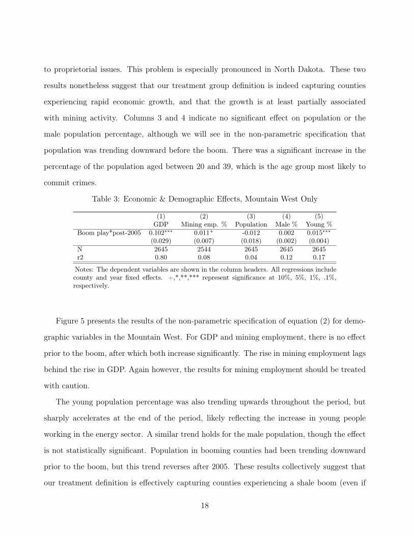
Table 3: Economic & Demographic Effects, Mountain West Only
(1) (2) (3) (4) (5)GDP Mining emp. % Population Male % Young %
Boom play*post-2005 0.102∗∗∗ 0.011+ -0.012 0.002 0.015∗∗∗(0.029) (0.007) (0.018) (0.002) (0.004)
N 2645 2544 2645 2645 2645r2 0.80 0.08 0.04 0.12 0.17
Notes: The dependent variables are shown in the column headers. All regressions includecounty and year fixed effects. +,*,**,*** represent significance at 10%, 5%, 1%, .1%,respectively.
Figure 5 presents the results of the non-parametric specification of equation (2) for demo-
graphic variables in the Mountain West. For GDP and mining employment, there is no effect
prior to the boom, after which both increase significantly. The rise in mining employment lags
behind the rise in GDP. Again however, the results for mining employment should be treated
with caution.
The young population percentage was also trending upwards throughout the period, but
sharply accelerates at the end of the period, likely reflecting the increase in young people
working in the energy sector. A similar trend holds for the male population, though the effect
is not statistically significant. Population in booming counties had been trending downward
prior to the boom, but this trend reverses after 2005. These results collectively suggest that
our treatment definition is effectively capturing counties experiencing a shale boom (even if
18
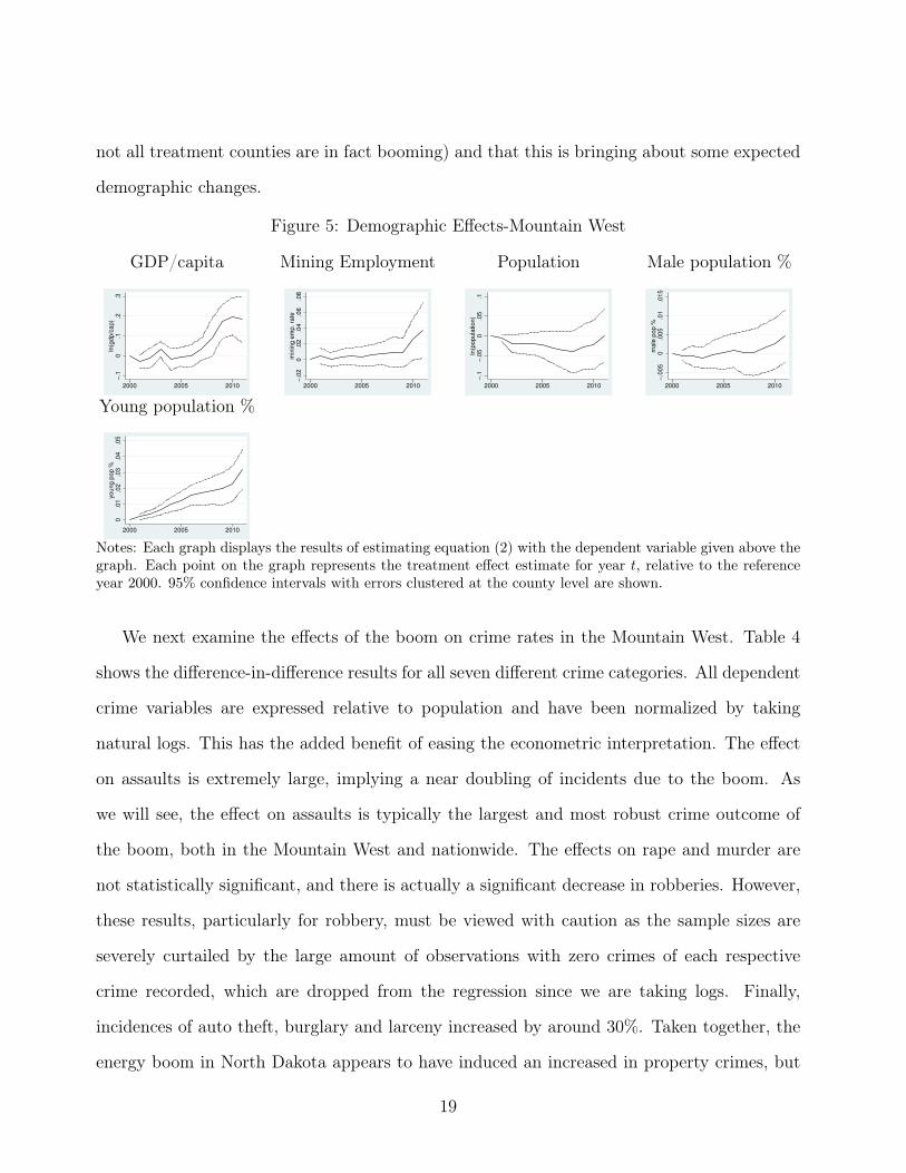
not all treatment counties are in fact booming) and that this is bringing about some expected
demographic changes.
Figure 5: Demographic Effects-Mountain West
GDP/capita
−.1
0.1
.2.3
ln(g
dp
/ca
p)
2000 2005 2010
Mining Employment
−.0
20
.02
.04
.06
.08
min
ing
em
p.
rate
2000 2005 2010
Population
−.1
−.0
50
.05
.1ln
(po
pu
latio
n)
2000 2005 2010
Male population %
−.0
05
0.0
05
.01
.01
5m
ale
po
p %
2000 2005 2010
Young population %
0.0
1.0
2.0
3.0
4.0
5yo
un
g p
op
%
2000 2005 2010
Notes: Each graph displays the results of estimating equation (2) with the dependent variable given above thegraph. Each point on the graph represents the treatment effect estimate for year t, relative to the referenceyear 2000. 95% confidence intervals with errors clustered at the county level are shown.
We next examine the effects of the boom on crime rates in the Mountain West. Table 4
shows the difference-in-difference results for all seven different crime categories. All dependent
crime variables are expressed relative to population and have been normalized by taking
natural logs. This has the added benefit of easing the econometric interpretation. The effect
on assaults is extremely large, implying a near doubling of incidents due to the boom. As
we will see, the effect on assaults is typically the largest and most robust crime outcome of
the boom, both in the Mountain West and nationwide. The effects on rape and murder are
not statistically significant, and there is actually a significant decrease in robberies. However,
these results, particularly for robbery, must be viewed with caution as the sample sizes are
severely curtailed by the large amount of observations with zero crimes of each respective
crime recorded, which are dropped from the regression since we are taking logs. Finally,
incidences of auto theft, burglary and larceny increased by around 30%. Taken together, the
energy boom in North Dakota appears to have induced an increased in property crimes, but
19
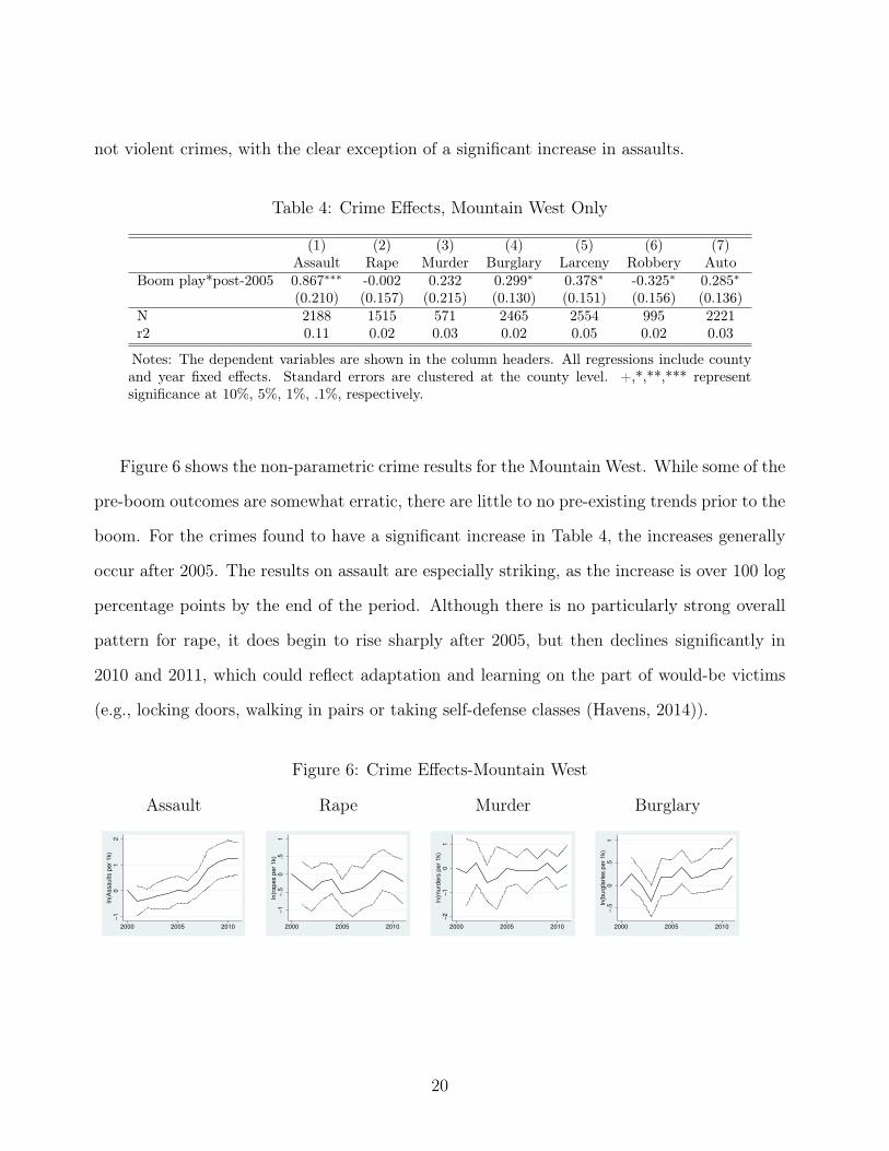
not violent crimes, with the clear exception of a significant increase in assaults.
Table 4: Crime Effects, Mountain West Only
(1) (2) (3) (4) (5) (6) (7)Assault Rape Murder Burglary Larceny Robbery Auto
Boom play*post-2005 0.867∗∗∗ -0.002 0.232 0.299∗ 0.378∗ -0.325∗ 0.285∗(0.210) (0.157) (0.215) (0.130) (0.151) (0.156) (0.136)
N 2188 1515 571 2465 2554 995 2221r2 0.11 0.02 0.03 0.02 0.05 0.02 0.03
Notes: The dependent variables are shown in the column headers. All regressions include countyand year fixed effects. Standard errors are clustered at the county level. +,*,**,*** representsignificance at 10%, 5%, 1%, .1%, respectively.
Figure 6 shows the non-parametric crime results for the Mountain West. While some of the
pre-boom outcomes are somewhat erratic, there are little to no pre-existing trends prior to the
boom. For the crimes found to have a significant increase in Table 4, the increases generally
occur after 2005. The results on assault are especially striking, as the increase is over 100 log
percentage points by the end of the period. Although there is no particularly strong overall
pattern for rape, it does begin to rise sharply after 2005, but then declines significantly in
2010 and 2011, which could reflect adaptation and learning on the part of would-be victims
(e.g., locking doors, walking in pairs or taking self-defense classes (Havens, 2014)).
Figure 6: Crime Effects-Mountain West
Assault
−1
01
2ln
(Assa
ults p
er
1k)
2000 2005 2010
Rape
−1
−.5
0.5
1ln
(ra
pe
s p
er
1k)
2000 2005 2010
Murder
−2
−1
01
ln(m
urd
ers
pe
r 1
k)
2000 2005 2010
Burglary
−.5
0.5
1ln
(bu
rgla
rie
s p
er
1k)
2000 2005 2010
20
Robbery
−1
−.5
0.5
1ln
(ro
bb
erie
s p
er
1k)
2000 2005 2010
Larceny
−.5
0.5
1ln
(la
rce
nie
s p
er
1k)
2000 2005 2010
Auto Theft
−.5
0.5
11
.5ln
(au
to t
he
fts p
er
1k)
2000 2005 2010
Notes: Each graph displays the results of estimating equation (2) with the dependent variable given above thegraph. Each point on the graph represents the treatment effect estimate for year t, relative to the referenceyear 2000. 95% confidence intervals with errors clustered at the county level are shown.
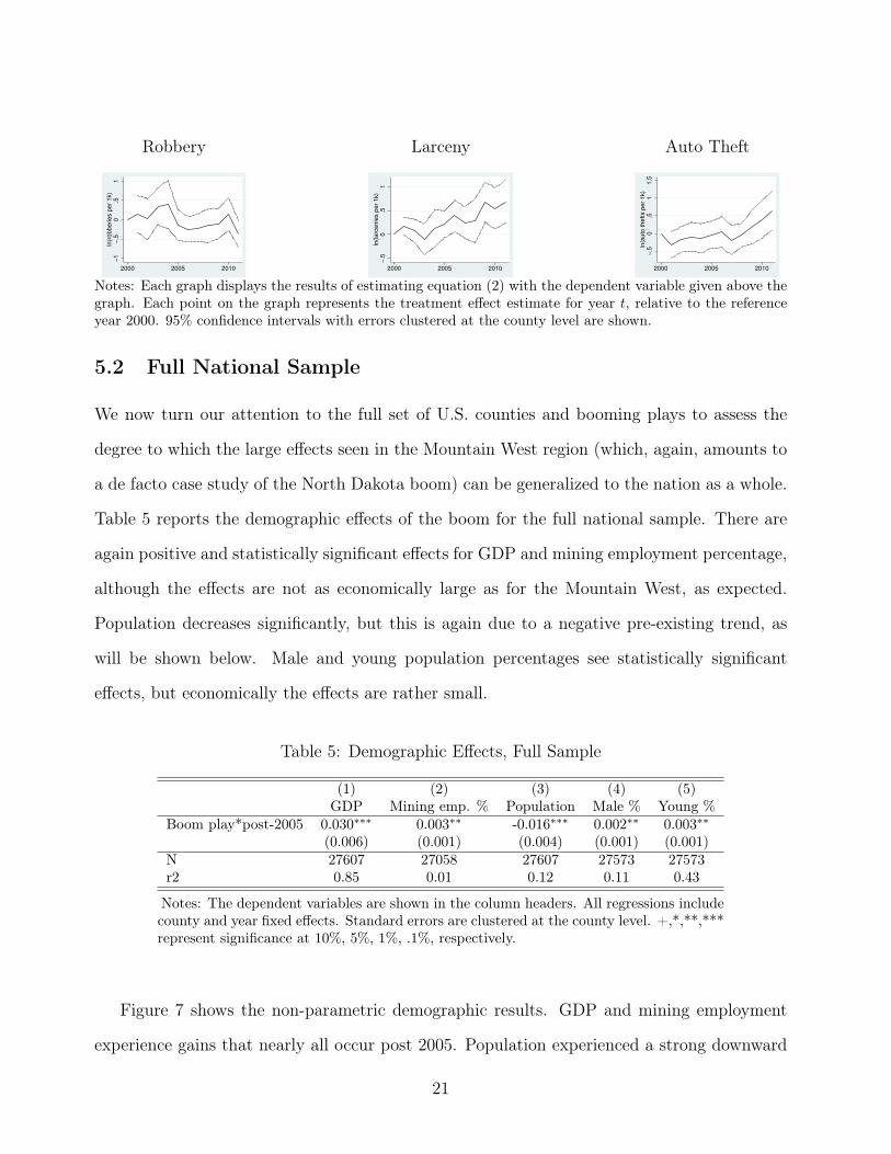
5.2 Full National Sample
We now turn our attention to the full set of U.S. counties and booming plays to assess the
degree to which the large effects seen in the Mountain West region (which, again, amounts to
a de facto case study of the North Dakota boom) can be generalized to the nation as a whole.
Table 5 reports the demographic effects of the boom for the full national sample. There are
again positive and statistically significant effects for GDP and mining employment percentage,
although the effects are not as economically large as for the Mountain West, as expected.
Population decreases significantly, but this is again due to a negative pre-existing trend, as
will be shown below. Male and young population percentages see statistically significant
effects, but economically the effects are rather small.
Table 5: Demographic Effects, Full Sample
(1) (2) (3) (4) (5)GDP Mining emp. % Population Male % Young %
Boom play*post-2005 0.030∗∗∗ 0.003∗∗ -0.016∗∗∗ 0.002∗∗ 0.003∗∗(0.006) (0.001) (0.004) (0.001) (0.001)
N 27607 27058 27607 27573 27573r2 0.85 0.01 0.12 0.11 0.43
Notes: The dependent variables are shown in the column headers. All regressions includecounty and year fixed effects. Standard errors are clustered at the county level. +,*,**,***represent significance at 10%, 5%, 1%, .1%, respectively.
Figure 7 shows the non-parametric demographic results. GDP and mining employment
experience gains that nearly all occur post 2005. Population experienced a strong downward
21

trend that ceased in the last 3 years of the sample, likely due to the energy boom. Young and
male percentages, and to a lesser extent mining employment, followed a steady upward trend
throughout the period. One advantage of the previous mountain west specification is that
treatment counties experienced the energy boom at the same time, i.e., the Bakken boomed
at once. Relaxing the analysis to the full sample case adds more noise to the model as different
plays were explored and developed at various times (the majority occurring post 2005). This
may help explain some of the upward trends present in Figure 7.
Figure 7: Demographic Effects-Full Sample
GDP/capita
−.0
50
.05
.1ln
(gd
p/c
ap
)
2000 2005 2010
Mining Employment
0.0
05
.01
.01
5m
inin
g e
mp
. ra
te
2000 2005 2010
Population
−.0
4−
.03
−.0
2−
.01
0ln
(po
pu
latio
n)
2000 2005 2010
Male population %
0.0
02
.00
4.0
06
ma
le p
op
%
2000 2005 2010
Young population %
0.0
02
.00
4.0
06
.00
8.0
1yo
un
g p
op
%
2000 2005 2010
Notes: Each graph displays the results of estimating equation (2) with the dependent variable given above thegraph. Each point on the graph represents the treatment effect estimate for year t, relative to the referenceyear 2000. 95% confidence intervals with errors clustered at the county level are shown.
We next examine effects on crime for the full national sample, which is our main baseline
set of results. Table 6 gives the results from the estimation of equation (1). Consistent with
our expectations, the magnitudes are lower than for the Mountain West region. There are,
however, positive and statistically significant effects for all seven crime categories, with effects
ranging from 5.3-11.9 percentage points, and assault again experiencing the largest effects.
Figure 8 shows the non-parametric crime results for the national sample. In all cases
average crime rates are clearly higher in the post-boom period, although for some crimes
22

Table 6: Crime Effects, Full Sample
(1) (2) (3) (4) (5) (6) (7)Assault Rape Murder Burglary Larceny Robbery Auto
Boom play*post-2005 0.119∗∗ 0.070+ 0.089∗ 0.053+ 0.102∗∗∗ 0.069∗ 0.061∗(0.037) (0.037) (0.035) (0.031) (0.029) (0.032) (0.029)
N 26463 21968 13198 27245 27352 19967 26160r2 0.09 0.01 0.00 0.00 0.01 0.01 0.06
Notes: The dependent variables are shown in the column headers. All regressions include countyand year fixed effects. Standard errors are clustered at the county level. +,*,**,*** representsignificance at 10%, 5%, 1%, .1%, respectively.
much of the increase comes before 2005. The main exception to this is assault, which has the
largest effects and has nearly all of the increases occur in the post-boom period.
Figure 8: Crime Effects-Full Sample
Assault
−.2
−.1
0.1
.2.3
ln(A
ssa
ults p
er
1k)
2000 2005 2010
Rape
−.1
0.1
.2.3
ln(r
ap
es p
er
1k)
2000 2005 2010
Murder
−.2
0.2
.4ln
(mu
rde
rs p
er
1k)
2000 2005 2010
Burglary
−.2
−.1
0.1
.2ln
(bu
rgla
rie
s p
er
1k)
2000 2005 2010
Robbery
−.1
0.1
.2.3
.4ln
(ro
bb
erie
s p
er
1k)
2000 2005 2010
Larceny
−.1
0.1
.2ln
(la
rce
nie
s p
er
1k)
2000 2005 2010
Auto Theft−
.10
.1.2
ln(a
uto
th
eft
s p
er
1k)
2000 2005 2010
Notes: Each graph displays the results of estimating equation (2) with the dependent variable given above thegraph. Each point on the graph represents the treatment effect estimate for year t, relative to the referenceyear 2000. 95% confidence intervals with errors clustered at the county level are shown.
To provide additional context to the results, we run a specification very similar to equation
(2), except with each booming play by year interaction term included, rather than excluding
the year 2000. In this specification, each interaction term will show the absolute conditional
difference in outcomes between treatments and controls, rather than the differences relative
to the reference year 2000. Removing county fixed effects is also necessary to get absolute
23
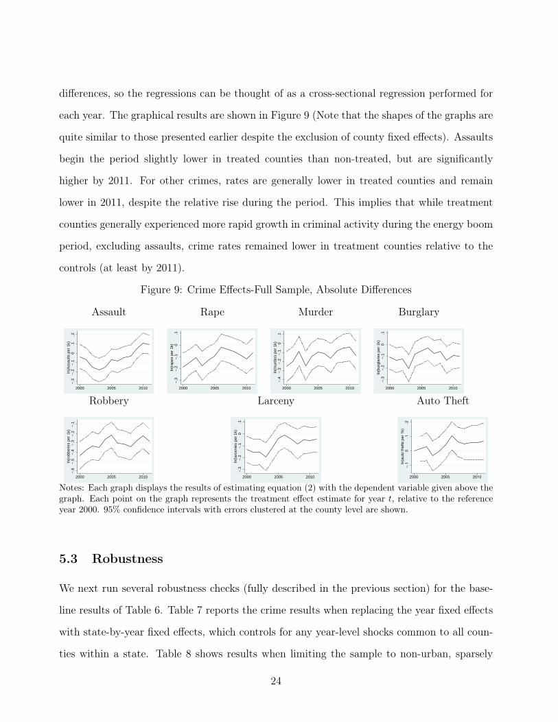
differences, so the regressions can be thought of as a cross-sectional regression performed for
each year. The graphical results are shown in Figure 9 (Note that the shapes of the graphs are
quite similar to those presented earlier despite the exclusion of county fixed effects). Assaults
begin the period slightly lower in treated counties than non-treated, but are significantly
higher by 2011. For other crimes, rates are generally lower in treated counties and remain
lower in 2011, despite the relative rise during the period. This implies that while treatment
counties generally experienced more rapid growth in criminal activity during the energy boom
period, excluding assaults, crime rates remained lower in treatment counties relative to the
controls (at least by 2011).
Figure 9: Crime Effects-Full Sample, Absolute Differences
Assault
−.3
−.2
−.1
0.1
.2ln
(Ass
aults
per
1k)
2000 2005 2010
Rape
−.3
−.2
−.1
0.1
ln(r
apes
per
1k)
2000 2005 2010
Murder
−.4
−.3
−.2
−.1
0.1
ln(m
urde
rs p
er 1
k)
2000 2005 2010
Burglary
−.3
−.2
−.1
0.1
ln(b
urgl
arie
s pe
r 1k
)
2000 2005 2010
Robbery
−.6
−.5
−.4
−.3
−.2
−.1
ln(r
obbe
ries
per
1k)
2000 2005 2010
Larceny
−.3
−.2
−.1
0.1
ln(la
rcen
ies
per
1k)
2000 2005 2010
Auto Theft−
.10
.1.2
ln(a
uto
th
eft
s p
er
1k)
2000 2005 2010
Notes: Each graph displays the results of estimating equation (2) with the dependent variable given above thegraph. Each point on the graph represents the treatment effect estimate for year t, relative to the referenceyear 2000. 95% confidence intervals with errors clustered at the county level are shown.
5.3 Robustness
We next run several robustness checks (fully described in the previous section) for the base-
line results of Table 6. Table 7 reports the crime results when replacing the year fixed effects
with state-by-year fixed effects, which controls for any year-level shocks common to all coun-
ties within a state. Table 8 shows results when limiting the sample to non-urban, sparsely
24
populated counties. Table 9 presents results when omitting all North Dakota counties, thus
eliminating the most extreme case of the shale boom and rise in crimes. Finally, Table 10
reports results when redefining treatment counties as any for which the center lies above a
play, not just a booming play.
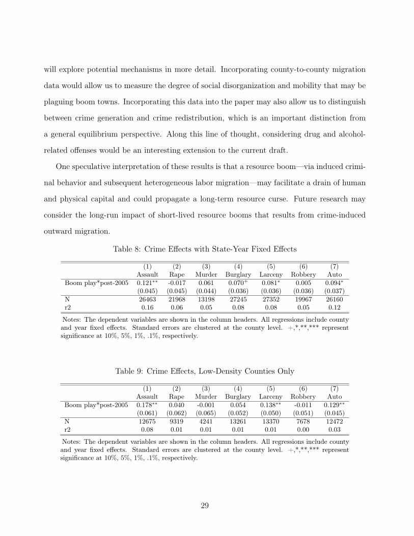
Controlling for state-year fixed effects causes the results for rape, murder and robbery to
become insignificant, while the other four outcomes remain significant. For the non-urban,
low density sample, the effect on assault increases substantially. For several other crimes, the
point estimates are similar but slightly smaller, which causes them to lose significance when
combined with the larger standard errors due to the smaller sample size. The effects when
omitting North Dakota are generally slightly smaller but remain significant, demonstrating
that the increase is not being driven solely by the extreme case of the Bakken play. Finally,
using all plays rather than booming plays for the identification causes the effects to become
smaller, as expected since this definition captures more non-booming counties, but the results
largely remain significant, mitigating concerns about the endogeneity of the booming play
treatment definition.
Overall, the positive effect on almost all types of crimes remain for all robustness checks,
though some lose statistical significance. The most robust effect is that for assault, which
remains large and significant in each specification. Since assaults are quite a serious crime
(recall we are only considering aggravated assaults, which strictly include assaults with the
intent to cause severe bodily injury, usually with use of a deadly weapon) occur much more
frequently than the other violent crimes studied (murder, rape, robbery), this is a highly
important result that local policy makers in current and prospective boom towns should
consider.
25
5.4 Do Criminals Disproportionately Move to Boom Towns?
Why do shale-rich booming communities experience elevated levels of criminal activity? Do
boom towns provide people with the opportunties and incentives to commit crimes, or do
criminals simply move to boomtowns? Ideally, one could examine the migratory behavior of
convicted fellons throughout the United States to test whether fellons move in disproportionate
numbers to boom towns. Such a federal registry does not exist, or is at least not publically
available. However, in 1996 the Sexual Offender Act was signed by President Bill Clinton. This
law, commonly refered to as “Megan’s Law” made public a registry of previously convicted
sexual offenders. We make use of this data to examine i) whether shale-rich counties in North
Dakota have a disproportionate number of sex offenders residing in them and ii) if sexual
offenders have moved in disproportionate numbers to live in shale-rich counties.
Data on sexual offenders living in North Dakota is available at sexoffender.nd.gov. This
data source details where each offender lives and the time and place of all previous offenses.
We omitt those offenders that are currently incarcerated as such individuals are not a threat
to society. A shortcoming of the analysis is that it is cross-sectional in nature, with a total of
53 data points (there are 53 counties in North Dakota), and registry data reflects up-to-date,
2014 records. While the results are quite striking, they should nonetheless be viewed with
caution as bias created from unobserved heterogeneity is an obvious concern when working
with cross-sectional data sets.
As a starting point, we individually regress the natural log of sex offenders per capita,
aggregated at the county level, on a variety of indicator variables that describe whether a
county is shale rich. We then restrict the data set by omitting those RSO’s that committed
the registering offense in another state. The implicit assumption being made is that offenders
commit crimes where they live. For example, an RSO that committed the registering offense
in New Hampshire in 1999, but currently lives in Williams, North Dakota, is assumed to have
previously lived in New Hampshire, but moved to North Dakota sometime between 1999 and
26
2014.
We use three different treatment definitions. First, we apply the methodology previously
employed in this paper, namely, we define a treatment county as one lying above the Bakken
shale formation. As previously discussed, this approach provides us with exogenous variation
in our treatment definition, but comes at the cost of added statistical noise. We therefore also
define a treatment county as one that was producing any oil in 2011 (the last year for which
we have county-level energy production data). Lastly, we define a county as being a “key” oil
producing county if it was one of the top five oil producers in the state of North Dakota in
2011.
The reuslts are given in Table 7. There is evidence that shale-rich North Dakota counties
have a disproportionately large number of registered sex offenders living in them. For all
treatment definitions, the coefficient of interest is positive, albeit insignificant when treatment
counties are defined as those lying above the Bakken shale play. The results are also eco-
nomically significant. For example, the top five oil producing counties had nearly twice as
many registered sex offenders living in them when compared to the control group of counties.
However, after restricting the data to only include those RSO’s that did not previously com-
mit a crime in another state, the results are insignficant or actually negative. This suggests
that perhaps the shale boom incentivised local and existing sex offenders to leave the boom
town. We consider this evidence that local shale booms have heterogeneously attracted labor
that may be more prone to have a criminal record. This of course is not to say that other
mechanisms, e.g., social disorder or inadequate police protection, are not also contributing to
the documented elevated levels of criminal activity.
27
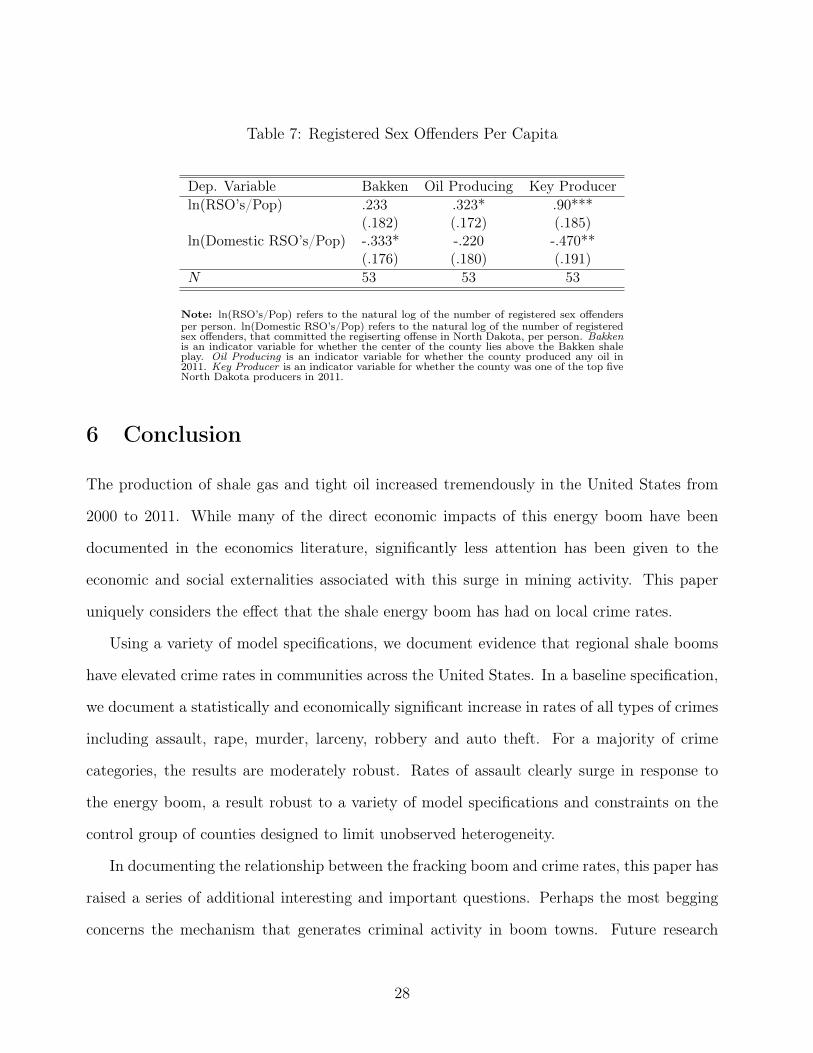
Table 7: Registered Sex Offenders Per Capita
Dep. Variable Bakken Oil Producing Key Producerln(RSO’s/Pop) .233 .323* .90***
(.182) (.172) (.185)ln(Domestic RSO’s/Pop) -.333* -.220 -.470**
(.176) (.180) (.191)N 53 53 53
Note: ln(RSO’s/Pop) refers to the natural log of the number of registered sex offendersper person. ln(Domestic RSO’s/Pop) refers to the natural log of the number of registeredsex offenders, that committed the regiserting offense in North Dakota, per person. Bakkenis an indicator variable for whether the center of the county lies above the Bakken shaleplay. Oil Producing is an indicator variable for whether the county produced any oil in2011. Key Producer is an indicator variable for whether the county was one of the top fiveNorth Dakota producers in 2011.
6 Conclusion
The production of shale gas and tight oil increased tremendously in the United States from
2000 to 2011. While many of the direct economic impacts of this energy boom have been
documented in the economics literature, significantly less attention has been given to the
economic and social externalities associated with this surge in mining activity. This paper
uniquely considers the effect that the shale energy boom has had on local crime rates.
Using a variety of model specifications, we document evidence that regional shale booms
have elevated crime rates in communities across the United States. In a baseline specification,
we document a statistically and economically significant increase in rates of all types of crimes
including assault, rape, murder, larceny, robbery and auto theft. For a majority of crime
categories, the results are moderately robust. Rates of assault clearly surge in response to
the energy boom, a result robust to a variety of model specifications and constraints on the
control group of counties designed to limit unobserved heterogeneity.
In documenting the relationship between the fracking boom and crime rates, this paper has
raised a series of additional interesting and important questions. Perhaps the most begging
concerns the mechanism that generates criminal activity in boom towns. Future research
28
will explore potential mechanisms in more detail. Incorporating county-to-county migration
data would allow us to measure the degree of social disorganization and mobility that may be
plaguing boom towns. Incorporating this data into the paper may also allow us to distinguish
between crime generation and crime redistribution, which is an important distinction from
a general equilibrium perspective. Along this line of thought, considering drug and alcohol-
related offenses would be an interesting extension to the current draft.
One speculative interpretation of these results is that a resource boom—via induced crimi-
nal behavior and subsequent heterogeneous labor migration—may facilitate a drain of human
and physical capital and could propagate a long-term resource curse. Future research may
consider the long-run impact of short-lived resource booms that results from crime-induced
outward migration.
Table 8: Crime Effects with State-Year Fixed Effects
(1) (2) (3) (4) (5) (6) (7)Assault Rape Murder Burglary Larceny Robbery Auto
Boom play*post-2005 0.121∗∗ -0.017 0.061 0.070+ 0.081∗ 0.005 0.094∗(0.045) (0.045) (0.044) (0.036) (0.036) (0.036) (0.037)
N 26463 21968 13198 27245 27352 19967 26160r2 0.16 0.06 0.05 0.08 0.08 0.05 0.12
Notes: The dependent variables are shown in the column headers. All regressions include countyand year fixed effects. Standard errors are clustered at the county level. +,*,**,*** representsignificance at 10%, 5%, 1%, .1%, respectively.
Table 9: Crime Effects, Low-Density Counties Only
(1) (2) (3) (4) (5) (6) (7)Assault Rape Murder Burglary Larceny Robbery Auto
Boom play*post-2005 0.178∗∗ 0.040 -0.001 0.054 0.138∗∗ -0.011 0.129∗∗(0.061) (0.062) (0.065) (0.052) (0.050) (0.051) (0.045)
N 12675 9319 4241 13261 13370 7678 12472r2 0.08 0.01 0.01 0.01 0.01 0.00 0.03
Notes: The dependent variables are shown in the column headers. All regressions include countyand year fixed effects. Standard errors are clustered at the county level. +,*,**,*** representsignificance at 10%, 5%, 1%, .1%, respectively.
29
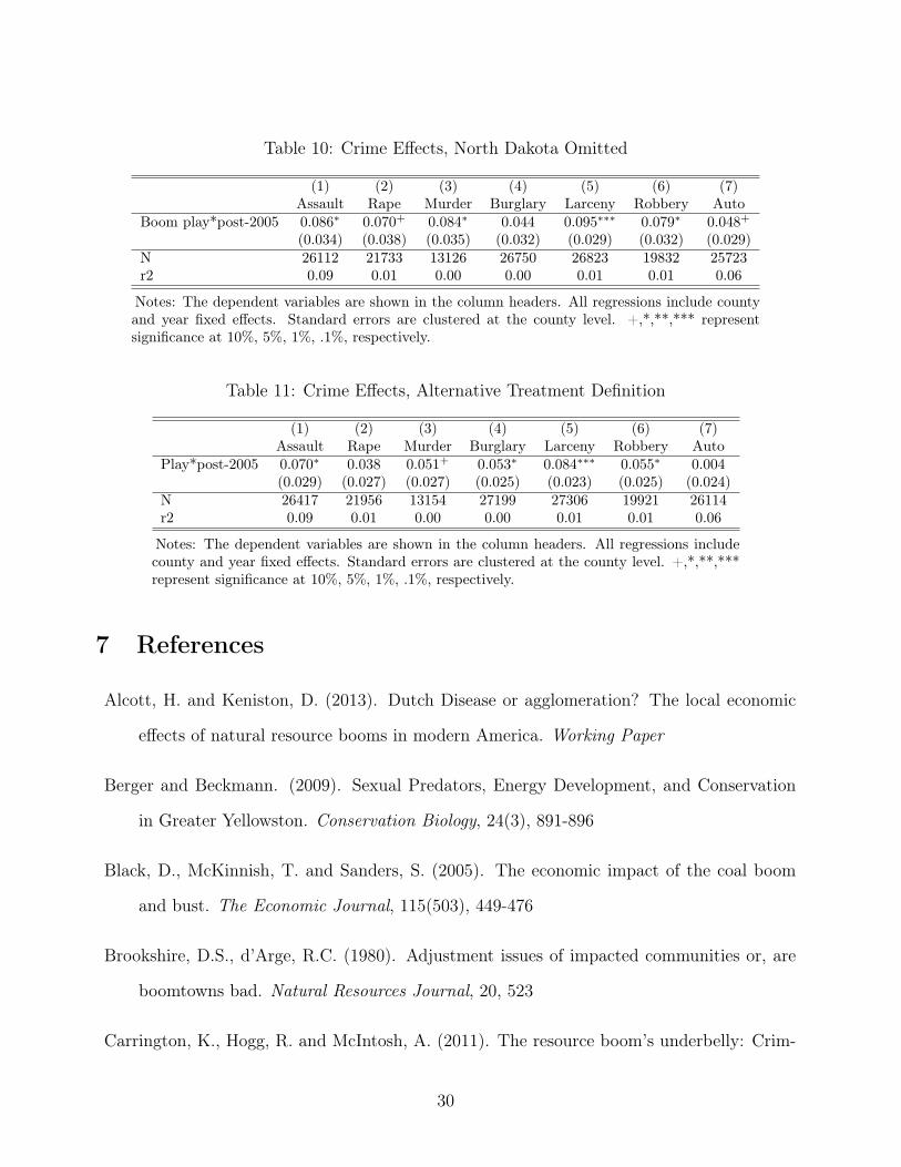
Table 10: Crime Effects, North Dakota Omitted
(1) (2) (3) (4) (5) (6) (7)Assault Rape Murder Burglary Larceny Robbery Auto
Boom play*post-2005 0.086∗ 0.070+ 0.084∗ 0.044 0.095∗∗∗ 0.079∗ 0.048+(0.034) (0.038) (0.035) (0.032) (0.029) (0.032) (0.029)
N 26112 21733 13126 26750 26823 19832 25723r2 0.09 0.01 0.00 0.00 0.01 0.01 0.06
Notes: The dependent variables are shown in the column headers. All regressions include countyand year fixed effects. Standard errors are clustered at the county level. +,*,**,*** representsignificance at 10%, 5%, 1%, .1%, respectively.
Table 11: Crime Effects, Alternative Treatment Definition
(1) (2) (3) (4) (5) (6) (7)Assault Rape Murder Burglary Larceny Robbery Auto
Play*post-2005 0.070∗ 0.038 0.051+ 0.053∗ 0.084∗∗∗ 0.055∗ 0.004(0.029) (0.027) (0.027) (0.025) (0.023) (0.025) (0.024)
N 26417 21956 13154 27199 27306 19921 26114r2 0.09 0.01 0.00 0.00 0.01 0.01 0.06
Notes: The dependent variables are shown in the column headers. All regressions includecounty and year fixed effects. Standard errors are clustered at the county level. +,*,**,***represent significance at 10%, 5%, 1%, .1%, respectively.
7 References
Alcott, H. and Keniston, D. (2013). Dutch Disease or agglomeration? The local economic
effects of natural resource booms in modern America. Working Paper
Berger and Beckmann. (2009). Sexual Predators, Energy Development, and Conservation
in Greater Yellowston. Conservation Biology, 24(3), 891-896
Black, D., McKinnish, T. and Sanders, S. (2005). The economic impact of the coal boom
and bust. The Economic Journal, 115(503), 449-476
Brookshire, D.S., d’Arge, R.C. (1980). Adjustment issues of impacted communities or, are
boomtowns bad. Natural Resources Journal, 20, 523
Carrington, K., Hogg, R. and McIntosh, A. (2011). The resource boom’s underbelly: Crim-
30
inological impacts of mining development. Australian & New Zealand Journal of Crim-
inology, 44(3), 335-354
Clausing, J. (2014, May 7). Booming New Mexico oil country faces challenges with crime,
deadly crashes, housing shortages. U.S. News & World Report. Retrieved from www.usnews.com
Di Tella, R. and Schargrodsky, E. (2004). Do police reduce crime? Estimates using the
allocation of police forces after a terrorist attack. The American Economic Review,
94(1), 115-133
Ecosystems Research Group. (2008). Sublette county socioeconomic study, Phase II—Final
report. Missoula, MT: Ecosystem Research Group, March, 2014
Ehrlich, I. (1973). Participation in illegitimate activities: A theoretical and empirical inves-
tigation. Journal of Political Economy, 81, 521-565
Eligon, J. (2013, January 15). An oil town where men are many, and women are hounded.
The New York Times. Retrieved from www.nytimes.com
Ellis, B. (2011, October 20). Double your salary in the middle of nowhere, North Dakota.
CNN Money. Retrieved from www.money.cnn.com
Ellis, B. (2011, October 26). Crime Turns oil boomtown into wild west. CNN Money.
Retrieved from www.money.cnn.com
Engquist, E. (2013, February 11). Fracking foes wield new weapon: crime. Crain’s New York
Business. Retrieved from www.crainsnewyork.com
Freudenburg, W.R. (1986). The density of acquaintanceship: An overlooked variable in
community research? American Journal of Sociology, 92(1), 27-63
Greenhouse, S. (2013, December 4). $15 Wage in fast food stirs debate on effects. The New
York Times. Retrieved from www.nytimes.com
31

Havens, J.R. (2014, March 28). Self Defense Course Empowers Women. KFYR-TV. Re-
trieved from www.kfyrtv.com
Healy, J. (2013, November 30). As Oil Floods Plains towns, Crime Pours In. New York
Times. Retrieved from www.nytimes.com
Hodur, N. and Bangsund, D. (2013, January). Population Estimates for the City of Williston,
Agribusiness and Applied Economics Report, vol. 707
Freudenburg, W.R., Jones, R.E. (1991). Criminal behavior and rapid community growth:
Examining the evidence 1. Rural Sociology, 56,4, 619-645
Kelly, M. (2000). Inequality and crime. Review of Economics and Statistics, 82(4), 530-539
Kowalski, L. and Zajac, G. (2012). A Preliminary Examination of Marcellus Shale Drilling
Activity and Crime Trends in Pennsylvania. Pennsylvania State University Justice Cen-
ter for Research.
Kubrin, C. andWeitzer, R. (2003). New Directions in Social Disorganization Theory. Journal
of Research in Crime and Delinquency, 40(374)
Luthra, A.D. (2006). The relationship of crime and oil development in the coastal regions of
Louisiana. Doctoral dissertation. Baton Rouge, LA Department of Sociology, Louisiana
State University. Retrieved March, 2014
Levy, M. (2014, October 26). Oil Boomtowns See Rise in Drunken Driving and Bar Fights
Threatening to Overwhelm Law Enforcement. Huffington Post Business. Retrieved
from www.huffingtonpost.com
Merton, R. (1938). Social Structure and Anomie. American Sociological Review, 3, 672-682
Michael, J. (2011). Crime up in North Dakota in 2011. The Bismarck Tribune
32
Pager, D. The mark of a criminal record. American Journal of Sociology, 108(5), 937-975
U.S. Energy Information Administration, Annual Energy Outlook 2014, April 2014.
Putz, A., Finken, A. and Goreham, G. (2011). Sustainability in natural resource-dependent
regions that experienced boom-bust-recovery cycles: lessons learned from a review of the
literature. Department of Sociology and Anthropology, North Dakota State University,
Fargo, ND.
Sampson, R.J and Groves, W.B. (1989). Community Structure and Crime: Testing Social-
Disorganization Theory. American Journal of Sociology, 94, 774-802
Shaw, C. and McKay, H. (1969). Juvenile Delinquency and Urban Areas. Chicago: Univer-
sity of Chicago press
Tewksbury, Richard, and Matthew Lees. Perceptions of sex offender registration: Collateral
consequences and community experiences, Sociological Spectrum, 26(3), 309-334
Weber, J. G. (2012). The effects of a natural gas boom on employment and income in
Colorado, Texas and Wyoming, Energy Economics, 34(5), 1580-1588
Wilkinson, K., Reynolds, R., Thompson, J., Ostresh, L. (1984). Violent crime in the Western
energy-development region. Sociological Perspectives, 241-256
33
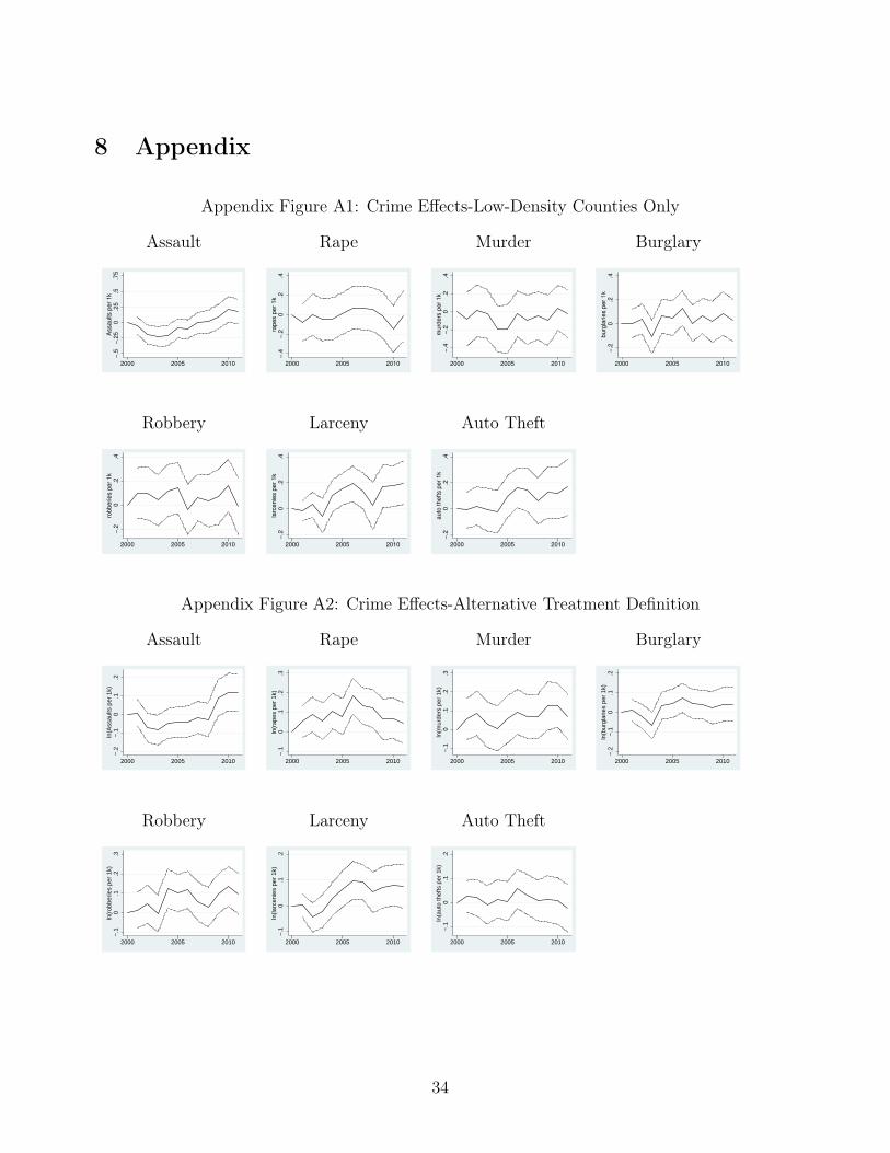
8 Appendix
Appendix Figure A1: Crime Effects-Low-Density Counties Only
Assault
−.5
−.2
50
.25
.5.7
5A
ssa
ults p
er
1k
2000 2005 2010
Rape
−.4
−.2
0.2
.4ra
pe
s p
er
1k
2000 2005 2010
Murder
−.4
−.2
0.2
.4m
urd
ers
pe
r 1
k
2000 2005 2010
Burglary
−.2
0.2
.4b
urg
larie
s p
er
1k
2000 2005 2010
Robbery
−.2
0.2
.4ro
bb
erie
s p
er
1k
2000 2005 2010
Larceny
−.2
0.2
.4la
rce
nie
s p
er
1k
2000 2005 2010
Auto Theft−
.20
.2.4
au
to t
he
fts p
er
1k
2000 2005 2010
Appendix Figure A2: Crime Effects-Alternative Treatment Definition
Assault
−.2
−.1
0.1
.2ln
(Ass
aults
per
1k)
2000 2005 2010
Rape
−.1
0.1
.2.3
ln(r
apes
per
1k)
2000 2005 2010
Murder
−.1
0.1
.2.3
ln(m
urde
rs p
er 1
k)
2000 2005 2010
Burglary
−.2
−.1
0.1
.2ln
(bur
glar
ies
per
1k)
2000 2005 2010
Robbery
−.1
0.1
.2.3
ln(r
obbe
ries
per
1k)
2000 2005 2010
Larceny
−.1
0.1
.2ln
(larc
enie
s pe
r 1k
)
2000 2005 2010
Auto Theft
−.1
0.1
.2ln
(aut
o th
efts
per
1k)
2000 2005 2010
34
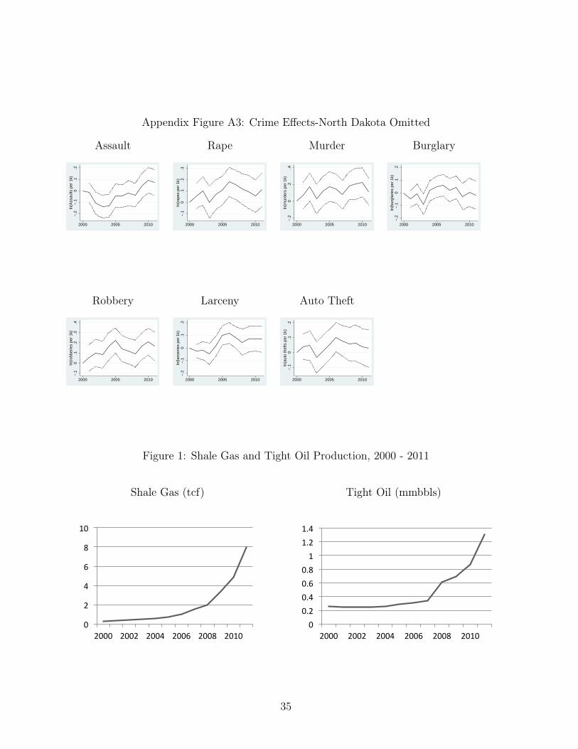
Appendix Figure A3: Crime Effects-North Dakota Omitted
Assault
−.2
−.1
0.1
.2ln
(Ass
aults
per
1k)
2000 2005 2010
Rape
−.1
0.1
.2.3
ln(r
apes
per
1k)
2000 2005 2010
Murder
−.2
0.2
.4ln
(mur
ders
per
1k)
2000 2005 2010
Burglary
−.2
−.1
0.1
.2ln
(bur
glar
ies
per
1k)
2000 2005 2010
Robbery
−.1
0.1
.2.3
.4ln
(rob
berie
s pe
r 1k
)
2000 2005 2010
Larceny
−.2
−.1
0.1
.2ln
(larc
enie
s pe
r 1k
)
2000 2005 2010
Auto Theft−
.10
.1.2
ln(a
uto
thef
ts p
er 1
k)
2000 2005 2010
Figure 1: Shale Gas and Tight Oil Production, 2000 - 2011
Shale Gas (tcf) Tight Oil (mmbbls)
!!!!!
Figure'1'
'!!!!! !!!!!!!!!!!!!!!! '
0'
2'
4'
6'
8'
10'
2000' 2002' 2004' 2006' 2008' 2010'
U.S.'Shale'Gas'Produc:on'(trillion'cubic'feet)'
0'0.2'0.4'0.6'0.8'1'
1.2'1.4'
2000' 2002' 2004' 2006' 2008' 2010'
U.S.'Tight'Oil'Produc:on'(million'barrles'per'day)'
'
35
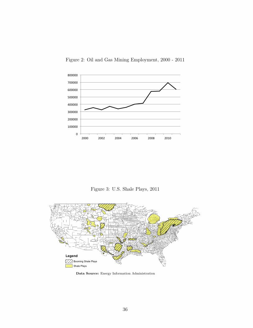
Figure 2: Oil and Gas Mining Employment, 2000 - 2011
!0"
100000"
200000"
300000"
400000"
500000"
600000"
700000"
800000"
2000" 2002" 2004" 2006" 2008" 2010"
Figure 3: U.S. Shale Plays, 2011
LegendBooming Shale Plays
Shale Plays
Data Source: Energy Information Administration
36