department of physics and astronomy · department of physics and astronomy university of heidelberg...

Department of Physics and Astronomy

University of Heidelberg

Diploma thesis

in Physics

submitted by

Bastian Höltkemeier

born in Bielefeld

2011

2D MOT as a source of a

cold atom target

This diploma thesis has been carried out by

Bastian Höltkemeier

at the

Physikalisches Institut

in Heidelberg

under the supervision of

Prof. Matthias Weidemüller

2D MOT as a source of a cold atom target

This thesis reports on the development, assembly and characterization of a two-dimensional magneto-optical trap (2D MOT). The 2D MOT is a particularly wellsuited source for cold atom targets due to a high brilliance with low ion background.We present the creation of a two-dimensional quadrupole field using permanentmagnets which, in combination with the use of opical fiber couplers leads to acompact and modular design. Our 2D MOT provides a well collimated beam of 4×109 atoms/s with a divergence of only 26mrad (FWHM), resulting in a brilliance of8×1012 atoms/(s · rad). The atoms have a mean velocity of 14m/s. The dependenceof the resulting velocity distribution and flux on the laser settings, magnetic fieldconfiguration and the use of a pushing laser beam is investigated. Furthermore, wepresent numerical simulations which reproduce the measured dependencies and thetotal atom flux.

2D MOT als Atomquelle für ein kaltes Target

In dieser Arbeit wird der Aufbau und die Realisierung einer zweidimensionalenmagneto-optischen Falle (2D MOT) als Quelle ultrakalter Atome beschrieben. Auf-grund hoher Brillanz und geringem Hintergrund eignet sich diese Quelle insbeson-dere zum Laden einer dreidimensionalen magneto-optischen Falle (3D MOT), welcheals Target für Ion-Atom Stöße dient. Gezeigt wird unter Anderem die Realisierungeines magnetischen Quadrupolfelds durch Permanentmagneten. In Kombinationmit optischen Faserkopplern führt dies zu einem kompakten und modularen Auf-bau. Die 2D MOT erzeugt einen kollimierten Atomstrahl mit 4 × 109 Atomen/sund einer Divergenz von 26mrad (FWHM). Dies entspricht einer Brillanz von8× 1012 Atomen/(s · rad). Die mittlere Geschwindigkeit der Atome beträgt 14m/s.Die Abhängigkeit der Geschwindigkeitsverteilung und des Atomflusses von denLaserparametern, dem Magnetfeld und einem Pusher-Laserstrahl wird untersucht.Es wird ein theoretisches Modell vorgestellt, welches die gemessenen Abhängigkeitengut beschreibt.

Contents

1 Introduction 1

2 2D MOT as a source of cold atoms 5

2.1 Magneto optical trap . . . . . . . . . . . . . . . . . . . . . . . . . . . . 52.1.1 Interaction of light and atoms . . . . . . . . . . . . . . . . . . . 52.1.2 Laser cooling . . . . . . . . . . . . . . . . . . . . . . . . . . . . 62.1.3 Magneto-optical trap . . . . . . . . . . . . . . . . . . . . . . . . 9

2.2 Atom beam sources . . . . . . . . . . . . . . . . . . . . . . . . . . . . . 112.2.1 Oven . . . . . . . . . . . . . . . . . . . . . . . . . . . . . . . . . 122.2.2 Zeeman slower . . . . . . . . . . . . . . . . . . . . . . . . . . . . 132.2.3 Double MOT systems and LVIS . . . . . . . . . . . . . . . . . . 142.2.4 2D MOT . . . . . . . . . . . . . . . . . . . . . . . . . . . . . . . 14

2.3 Model of a 2D MOT . . . . . . . . . . . . . . . . . . . . . . . . . . . . 172.3.1 Model for the light force . . . . . . . . . . . . . . . . . . . . . . 182.3.2 Atom trajectories . . . . . . . . . . . . . . . . . . . . . . . . . . 19

3 Realization of the 2D MOT 23

3.1 Laser system . . . . . . . . . . . . . . . . . . . . . . . . . . . . . . . . 233.1.1 Cooling laser . . . . . . . . . . . . . . . . . . . . . . . . . . . . 253.1.2 Repumping laser . . . . . . . . . . . . . . . . . . . . . . . . . . 273.1.3 Laser cubes . . . . . . . . . . . . . . . . . . . . . . . . . . . . . 28

3.2 2D MOT setup . . . . . . . . . . . . . . . . . . . . . . . . . . . . . . . 283.2.1 Bellow with differential pumping tube . . . . . . . . . . . . . . . 293.2.2 Glascell . . . . . . . . . . . . . . . . . . . . . . . . . . . . . . . 303.2.3 Optics . . . . . . . . . . . . . . . . . . . . . . . . . . . . . . . . 31

3.3 Magnetic field design . . . . . . . . . . . . . . . . . . . . . . . . . . . . 333.3.1 Permanent magnets . . . . . . . . . . . . . . . . . . . . . . . . . 343.3.2 Magnetization . . . . . . . . . . . . . . . . . . . . . . . . . . . . 353.3.3 Setup of the magnets . . . . . . . . . . . . . . . . . . . . . . . . 36

4 Characterization of the atom beam 41

4.1 Test setup . . . . . . . . . . . . . . . . . . . . . . . . . . . . . . . . . . 414.1.1 Measurement of the velocity distribution . . . . . . . . . . . . . 434.1.2 Measurement of the flux . . . . . . . . . . . . . . . . . . . . . . 45

4.2 Beam divergence . . . . . . . . . . . . . . . . . . . . . . . . . . . . . . 464.3 Dependence on laser settings . . . . . . . . . . . . . . . . . . . . . . . . 48

4.3.1 Detuning cooling laser . . . . . . . . . . . . . . . . . . . . . . . 484.3.2 Power cooling laser . . . . . . . . . . . . . . . . . . . . . . . . . 49

I

Contents

4.3.3 Repumping laser . . . . . . . . . . . . . . . . . . . . . . . . . . 524.3.4 Pushing laser . . . . . . . . . . . . . . . . . . . . . . . . . . . . 524.3.5 Counter-propagating pushing beam . . . . . . . . . . . . . . . . 59

4.4 Influence of partial pressure and length of cooling volume . . . . . . . . 604.5 Magnetic fields . . . . . . . . . . . . . . . . . . . . . . . . . . . . . . . 63

4.5.1 Magnetic field gradient . . . . . . . . . . . . . . . . . . . . . . . 634.5.2 Compensation coils . . . . . . . . . . . . . . . . . . . . . . . . . 63

4.6 Beam size . . . . . . . . . . . . . . . . . . . . . . . . . . . . . . . . . . 65

5 Conclusion and Outlook 67

List of Figures 70

Bibliography 74

II

1 Introduction

State of the art experiments on ultracold quantum gases involve a three-dimensional

magneto-optical trap (3D MOT) as a first cooling procedure which is a typical starting

point for further experiments such as evaporative cooling or trapping in optical lattices.

These schemes require favorable initial conditions such as low starting temperatures,

high atom numbers and long lifetimes of the atoms in the trap. A typical limitation

is the collisions with background gas atoms, making it necessary to perform these

experiments under ultra-high vacuum (UHV) conditions. However, low vapor pressure

results in a very inefficient loading from background vapor. Instead, cold atom beams

can be used as a source to achieve short loading times and high atom numbers in the

MOT without compromising UHV conditions.

Since the first demonstration of a laser cooled atom beam by Philipps and Metcalf

[1], new methods for producing high brilliance cold atom beam sources have been

under investigation. One of the most common techniques is to decelerate a thermal

atom beam with the radiation pressure from a resonant laser beam. The atoms are

kept on resonance either by chirping the laser frequency (chirped slower) [2] or by

spatially varying magnetic fields (Zeeman slower) [3]. These kind of setups produce

bright atom beams at low temperatures, but require a great engineering effort. The

main drawback is that the atom beams have a large transverse velocity spread since

the atoms are only cooled in longitudinal direction. In order to avoid the increasing

beam divergence at low longitudinal velocities, more sophisticated schemes for these

slowers have been developed [4].

Beams with even lower mean velocities that are both longitudinally and transversely

cooled can be provided by MOT sources. For most alkali metals they are commonly

used alternatives providing advantages such as a compact setup, well collimated beams

and low laser power. In a seperate chamber atoms are trapped in a vapor cell MOT

from where they can be extracted. The first breakthrough of this method was realized

by Lu et al. [5] who extracted the atoms by a power imbalance in two of the MOT’s

cooling lasers. This low velocity intense source (LVIS) provides an bright atom beam

at very low temperatures, with only a small thermal background.

Another approach is the two-dimensional magneto-optical trap (2D MOT). Atoms

are cooled and trapped in two dimensions, leading to a well collimated cold atom beam

in the third dimension. The atoms are transferred to the science chamber through a

1

CHAPTER 1. INTRODUCTION

small aperture which at the same time is used for differential pumping making this

system perfectly suited for loading a 3D MOT under UHV conditions. During the last

15 years, 2D MOTs for rubidium [6, 7], potassium [8], cesium [9, 10, 11], sodium [12]

and lithium [13] have been developed and the characteristics of the produced beams

have been investigated in experiment and theory. Most of the 2D MOTs’ features can

be qualitatively explained on the basis of simple models, yet some details are still not

understood to a satisfying degree.

In this thesis we report on the setup of a 2D MOT which will be used to load a cold

target for the investigation of atoms-ion collisions. The experiment will focus on the

dynamics in multiple electron transfer between neutral atoms and highly charged ions.

For this purpose the setup will be implemented in the HITRAP beamline at GSI where

ions up to Ur92+ will be available. The momentum transferred during these collisions

is investigated using “Recoil Ion Momentum Spectroscopy” (RIMS) [14]. Depending

on the projectile energy, the collision of a rubidium atom and a highly charged ion

can either lead to ionization of the target atom or to charge transfer. Using RIMS,

the measured three-dimensional momentum distribution reveals the dynamics during

the collision. The ion’s longitudinal momentum is proportional to the total change in

binding energies of the transfered electrons (Q-value) while the transverse momentum

contains information about the scattering angle of the collisions. The resolution of this

technique depends strongly on the initial velocity of the target atoms as the momentum

transfer between the ion and the atom is very small. Therefore, the target has to be

cold. In the case of light noble gases (He, Ne, Ar), the targets are cooled by supersonic

expansion. Cold targets with other species can be provided by 3D MOTs [15]. Using

the atomic beam from a 2D MOT might also present an alternative approach.

In our setup, rubidium atoms are trapped in a MOT which is positioned at the

center of a RIMS detector. The cross sections of the investigated collisions are in the

order of 10−15 cm2, depending on the number of electrons transfered [16]. Hence, a

large number of target atoms is needed to achieve adequate statistics in reasonable

run-times. At the same time, the background should be small during the measure-

ments. Therefore, the implementation of a 2D MOT as a source for the 3D MOT

serves multiple purposes. It allows to keep a very low pressure in the experimental

chamber, provides a large number of cold atoms leading to short loading times and no

background ions.

We present in this work the development, assembly and characterization of a com-

pact and modular 2D MOT setup. The efficiency of different loading schemes for 3D

MOTs will be discussed in the first part of chapter 2. Section 2.1 will give a short

introduction on the working principle of a MOT. Based on this section 2.2 will present

2

different atom beam sources and discuss their advantages and disadvantages for load-

ing a MOT. In section 2.3 a model that can describe some of the key features of a 2D

MOT will be presented.

The third chapter will give a detailed description of the construction and assembly

of the 2D MOT including a new laser system (section 3.1) and a compact and modular

design of the 2D MOT itself (section 3.2).

After assembly, the 2D MOT was characterized on a test chamber (section 4.1)

where the dependency on the atom flux and the velocity distribution on various pa-

rameters was investigated. These dependencies are best understood when comparing

the measurements to a numerical simulation. All the measurements and results from

the model are presented and discussed in sections 4.2 to 4.6. In particular, we inves-

tigate in detail the influence of an additional laser beam in the direction of the atom

beam (section 4.3.4 and 4.3.5).

3

2 2D MOT as a source of cold

atoms

In the first part of this chapter the principle of a magneto optical trap (MOT) will be

explained, followed by an overview of some of the most common atom beam sources

which are used to load such a trap. A 2D MOT is one of these beam sources and

in the last part of this chapter a theoretical model to describe a 2D MOT will be

introduced. It can be used to simulate the dependence of the atom flux on various

important parameters of the 2D MOT.

2.1 Magneto optical trap

In a MOT atoms are cooled to temperatures of a few hundred µK by using a force of

near resonant laser light which arises form spontaneous scattering of photons by the

atoms. In the first section an overview over the interaction of light and atoms will

be given. Based on this, section 2.1.2 will show how this interaction can lead to a

cooling of the atoms. This can be used to trap the atoms at the zero point a magnetic

quadrupole field (section 2.1.3).

2.1.1 Interaction of light and atoms

The interaction of light and atoms can be described as a periodically perturbed two-

level system [17]. This seems to be a strong simplification at first glance since all atoms

have a very complicated inner structure far from being a two-level system. But if the

light only couples to two of the atom’s energy levels as in the case of monochromatic

laser light, the two-level approximation becomes far more realistic.

Let us consider the simple case where a two level atom is in the ground state and at

rest. It is located in the light field of a monochromatic laser in resonance with the

atomic transition and is propagating in ~ez direction. Three processes can occur when

the atom interacts with the light field of a laser: spontaneous emission, stimulated

emission and absorption. Absorbing a photon, the atom receives the photon’s initial

momentum of ~~k giving it a kick in the direction ~ez of the laser. The atom is now in

5

CHAPTER 2. 2D MOT AS A SOURCE OF COLD ATOMS

the excited state and there are two different channels to decay back into the ground

state. It can either interact with the light field of the laser again and emit a photon

back in ~ez direction receiving a kick in the opposite direction (stimulated emission) or

it can spontaneously decay back to the ground state where the direction of the emitted

photon is random (spontaneous emission).

In the first case, the atom has the same momentum before and after the absorption

cycle. The momentum only differs while it is in the excited state. Nevertheless, it

is possible to create a setup where this process creates a net force on the atom. If

the light field has an intensity gradient and is far detuned from the atomic transition,

there is a force pointing towards the intensity minimum (in case of blue detuning)

or the intensity maximum (in the case of red detuning) of the light field [18]. This

phenomenon is used in dipole traps where atoms are directly trapped in the light field

of a laser.

If the atom spontaneously decays back into the ground state instead, the light is

scattered isotropically. Averaging over many cycles where the atom absorbs photons

in ~ez direction and emits spontaneously in all directions, there is a net force ~Fspon

acting on the atom in the direction of the laser ~ez. This is the so called spontaneous

or scattering force which can be used to cool and in combination with a magnetic field

also trap atoms.

2.1.2 Laser cooling

The spontaneous force acts on the atoms in the propagation direction of the laser

beam. If the laser is on resonance with the atomic transition, this affects only atoms

at rest or very slow atoms. Due to the Doppler shift atoms at higher velocities are

no longer in resonance with the laser light. They see the laser at a frequency of

ω = ωres − ~k~v. Here ωres is the resonance frequency of the atomic transition, ~k is

the wave vector of the laser and ~v is the atoms velocity. Analogously, if the laser is

detuned from the transition by δ, atoms with a velocity of ~v = δ/~k are on resonance.

This means that the total detuning is given by

δtot = δ + ~k~v . (2.1)

But also atoms that are not precisely on resonance can interact with the light field

because of the finite natural linewidth of the transition. The velocity classes which

are still affected by the light field of the laser depend on the lasers intensity and its

detuning [19]:

~Fspon(~v) = ~~kΓ

2

I/I0

1 + I/I0 + (2(δ − ~k~v/Γ))2(2.2)

6

2.1. MAGNETO OPTICAL TRAP

00.10.20.30.40.50.60.70.80.9

1

-60 -40 -20 0 20 40 60scatt

eri

ng

rate

γ(Γ/2)

velocity v (m/s)

I = 200 I0I = 20 I0I = 5 I0I = I0

Figure 2.1 Scattering rate as a function of the atom velocity for different laser inten-sities. The scattering rate is shown as a fraction of the maximum scattering rateΓ/2. At high intensities the scattering rate saturates at γ = Γ/2.

where Γ is the natural linewidth of the transition, I is the laser intensity and I0 is

the saturation intensity. The saturation intensity is based on the fact that the rate

at which the atoms scatter photons (scattering rate) only increases linearly at low

intensities. At higher intensities, stimulated emission is the dominant process and

the spontaneous emission levels out at a maximum scattering rate of γ = Γ/2. The

saturation intensity of an atomic resonance is defined as the laser intensity where the

scattering rate is half the maximum scattering rate γ(I0) = Γ/4. The scattering rate as

a function of the atoms velocity is shown in figure 2.1 where the laser is on resonance.

The saturation effect can be seen as the scattering rate for atoms at rest has almost

reached the maximum of Γ/2 at I = 20× I0. The only difference at higher intensities

is the widening of the peak which means that also atoms at higher velocities will be

affected by the light field. In order to understand the concept of laser cooling we now

want to consider an one dimensional system with counter propagating laser beams

along the x-axis. Both beams are shifted by the same detuning δ. The force of each

laser beams is given by:

~F±(~v) = ±~~kΓ

2

I/I0

1 + I/I0 + (2(δ ∓ ~k~v/Γ))2(2.3)

where ~F+/~F− are the forces resulting from the beam traveling in positive/negative

x-direction. The resulting total force ~Ftot = ~F+ + ~F− can be expanded in powers of~k~v/Γ:

~Ftot(~v) =8~k2δ

Γ

I/I01 + I/I0 + (2δ/Γ)2

~v + O((~k~v/Γ)4) . (2.4)

7


-0.1-0.08-0.06-0.04-0.02

00.020.040.060.080.1

-40 -20 0 20 40

Forc

eF

(N)

velocity v (m/s)

F+/F−

Ftot

Figure 2.2 Spontaneous force on atoms in the light field. Shown are the forces actingon the atoms by the single laser beams F+/F− and the resulting total force Ftot.The detuning is δ = 2Γ and I/I0 = 20.

For δ < 0, this describes a damping force with a positive damping coefficient thus

slowing down the atoms that are close to resonance. Figure 2.2 shows the complete

behavior of Ftot without neglecting any higher order terms. To slow down the atoms

they have to scatter multiple photons. An atom with an initial velocity of about 20

m/s has to scatter about 10000 photons to loose its momentum.

It is not possible to stop the atoms completely. So far, we assumed that the mo-

mentum gain due to spontaneous emission averages to zero because of its isotropic

nature. However, considering only the single momentum transfers due to spontaneous

emissions of single photons the atom will undergo a random walk in momentum space

with step size ~k. At low temperatures, this heating process competes against the

cooling mechanism due to absorption. At the so called Doppler temperature both

processes are balanced out. This temperature is given by [19]:

TDoppler =~Γ

2kB. (2.5)

The first temperature measurements on optically cooled and stored atoms already

contradicted this result by showing temperatures below the Doppler limit [20]. It was

shown that this discrepancy of theory and experiment is caused by the too rigorous

approximation of a two-level system. The physical limit for the temperature achievable

with laser cooling techniques is the recoil temperature of a single photon which is well

below the Doppler temperature.

8

2.1. MAGNETO OPTICAL TRAP

2.1.3 Magneto-optical trap

Figure 2.3 Setup of a 3D MOT. The atoms (red cloud in the center), are trappedin the light field of six orthogonal laser beams and the magnetic quadrupole fieldfrom a pair of magnetic coils. (Picture adapted from [21])

In order to trap atoms one has to find a way to make the velocity dependent spon-

taneous force spatially dependent as well. In a MOT this is achieved by adding a

magnetic field to the system. To understand how this can be used to trap atoms, a

two level system is considered once more. A linear magnetic field B(x) = B0 x with

a constant gradient B0 is applied lifting the degeneracy of the atom’s magnetic sub-

levels. In the simplest case, the ground state has an angular momentum of J = 0 and

the excited state has J = 1. This means that the excited state will split up into three

Zeemann levels (mJ = −1, 0, 1) with an energy of:

Ezeeman(mJ) = E0 + gJ µB mJ B0x (2.6)

with E0 being the energy of the inperturbed excited state, gJ the Lande factor, µB the

Bohr magneton and mJ the magnetic quantum number. This splitting of the excited

state’s energy levels also affects the spontaneous force. The overall detuning of the

laser from the atomic resonance is now given by

δtot = δ + ~k~v +gJµBmJB0x

~, (2.7)

where the last term takes the position dependent energy splitting of the excited state

into account. In this setup, the spontaneous force depends on the atomic sublevel the

9


Figure 2.4 Phasespace of neutral Rb atoms in the light field of a 3D MOT. Onlyatoms that are moving slowly enough can be captured in the MOT. The parame-ters for this simulation are δ = 2Γ and I/I=20. All heating effects are neglected.

atom is excited to:

~F±(~v, x) = ±~~kΓ

2

I/I0

1 + I/I0 + (2(δ ∓ ~k~v ± gJµBmJB0x/~)2. (2.8)

For the excitation to mJ = 0 this force is the same as in equation 2.3, but for the

excitation to mJ = 1 and mJ = −1 the force depends on the atoms’ position. This

can be used to trap the atoms in a similar way to the red detuning that was used to

cool the atoms. The red detuning causes the atoms to always interact more strongly

with the beam that is traveling against their own direction of propagation.

A similar effect occurs if a σ+/σ− polarization is applied to the beam coming from

the left/right so that the light selectively pumps the atoms to the mJ = −1/mJ = +1

state. This leads to a configuration where atoms at x < 0 interact more strongly

with the beam coming from the left and atoms at x > 0 with the beam from the

right. This effectively pushes the atoms to x = 0 where the different Zeeman levels are

degenerated again. Thus the atoms interact equally with both beams and the total

force vanishes.

Figure 2.4 shows the atoms trajectories in phase space. Both, the confinement in

10

2.2. ATOM BEAM SOURCES

velocity and in position space are clearly visible. The simulation also shows, that there

are certain limits to the capturing of the atoms. If they travel faster than a certain

velocity (capture velocity), they cannot be trapped. There is also a limitation on the

volume from which atoms can still be pulled into the trap but this cannot be seen in

the one dimensional phasespace since it is hard to miss something in a one dimensional

world.

In higher dimensions, the situation is far more complicated but the general principle

still holds (In section 2.3 an heuristic equation which can be used to model the spon-

taneous force in three dimensions as well, will be presented). In order to trap atoms in

our three dimensional world two more pairs of counter propagating laser beams along

with a magnetic field gradient have to be applied in the other two dimensions. Nowa-

days this technique is one of the standard tools in AMO physics and is successfully

used in labs all around the world.

The limited capture velocity makes the loading from background gas quiet inefficient.

At room temperature, the mean velocity of rubidium gas is about 280m/s. Typical

capture velocities are well below that [22] which means that most atoms in the gas are

too fast to be captured by the trap. For a capture velocity of 40m/s, only 0.33% of

the rubidium atoms are actually slow enough to be trapped. Another limitation when

loading from background vapor are losses due to collisions with background gas. Even

a single collision of a trapped atom with an atom at room temperature is sufficient

to remove it from the trap. For that reason, experiments with ultra-cold atoms have

to be carried out under ultra high vacuum (UHV) conditions. On one hand, it is

favorable to have a high partial pressure of the atoms one wants to trap leading to a

higher loading rate. On the other hand a higher partial pressure leads to an increased

loss rate due to collisions which outweighs the increase in the loading rate at high

pressures. This is why there has been a lot of research on creating slow atom beams

to overcome this problem.

2.2 Atom beam sources

To load a 3D MOT efficiently a high flux of slow atoms is needed. A good benchmark

for an atom beam is the total flux of atoms below the capture velocity of a 3D MOT.

It also has to be taken into account that the cooling volume of a 3D MOT is limited.

Therefore, the divergence of the atom beam is of great importance as well. In the

following some common cold atom sources are presented and their advantages and

disadvantages are briefly discussed.

11


(a) (b)

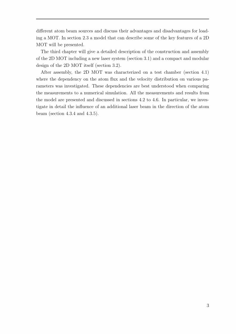
Figure 2.5 Atom beam from an oven. (a) Flux through area dA. All the atoms inthe gray cylinder will reach the area dA during the time dt. (b) Beam collimationwith an aperture.

2.2.1 Oven

One way to produce an atomic beam is to use an oven. This is basically just a reservoir

filled with rubidium gas with a hole through which atoms can leave the oven.

This process is called effusion and the flux of such an oven can easily be calculated

if the diameter of the exit-hole is much smaller than the mean free path length of

the atoms in the reservoir [23, 24]. In this case, the Maxwell-Boltzmann velocity

distribution can be used to describe the movement of the atoms because the hole is

too small to perturb the equilibrium in the reservoir. First, the number of atoms that

passes an infinitely small area dA which is part of the hole will be calculated. Let the

z-axis be the normal to this surface, then within the time interval [t, t + dt] from all

atoms with a velocity between [v, v+dv] and an azimuth angle between [θ, θ+dθ] and

[φ, φ + dφ] only those which are closer to the surface than vdt will reach dA. These

are all the atoms in a cylinder of volume dAvdt cos θ (see figure 2.5a). The number

of atoms within the considered velocity interval is given by fMB(v)d3v, where fMB(v)

is the Maxwell-Boltzmann distribution. Dividing by dA and dt gives the flux per unit

area:

Φ(v)d3v = cos θ v fMB(v) d3v . (2.9)

Integrating over all velocities with vz > 0 and over the area of the hole gives us the

total flux of atoms:

Φ = A

∫

vz>0

cos θ v fMB(v) d3v . (2.10)

This means that the atoms which leave the oven through the exit hole are not emitted

isotropically, but with p(θ) ∼ cos θ. Moreover, the mean velocity of the atoms in the

beam is not the same as the mean velocity of the atoms in the reservoir. The Maxwell-

Boltzmann distribution has a velocity dependence of fMB(v) ∼ v2 expmv2/(2kBT ) with

kB being the Boltzmann-constant, while in the beam fbeam(v) ∼ v3 expmv2/(2kBT ).

At a temperature of T = 300K a gas of Rubidium atoms has a mean velocity of

12


Figure 2.6 Zeeman Slower. A thermal atomic beam is decelerated by a counterpropagating resonant laser beam. In order to keep the laser on resonance a nonlinear magnetic field has to be applied.

vmean ≈ 273m/s whereas Rubidium atoms that leave the oven have a mean velocity

of vmean ≈ 321m/s.

The oven emits atoms into a solid angle of 2π. In order to get an atom beam with

a smaller divergence, one can place an aperture with radius rap at a distance l from

the exit hole (figure 2.5b). This way, only atoms that are emitted in a solid angle

of θ = arctan(rap/l) participate in the atom beam. As mentioned before, only atoms

that are emitted in a solid angle of [0, θmax] which covers the cooling volume of the 3D

MOT, can be trapped. The total flux of atoms emitted in this angle is given by

Φ = A

∫ θmax

θ=0

∫ 2π

φ=0

∫

∞

v=0

cos(θ) sin(θ) v fMB(v) dvdφdθ . (2.11)

For typical MOT sizes, this leads to a flux of a few 109 atoms/s, at room temperature.

The number of atoms that can be trapped is a lot smaller, since the mean velocity of

the oven beam is about 321m/s, whereas typical capture velocities are in the range

of 25-40m/s. This means that only about 0.05% of the atoms are slow enough to be

trapped, leading to a loading flux of a few 106 atoms/s into the MOT. The following

section describes more efficient techniques for providing high fluxes at low velocities

2.2.2 Zeeman slower

A Zeeman slower uses a beam of thermal atoms as a starting point and decelerates

them. The thermal beam can be provided by an oven like the one just discussed. In

order to decelerate the atoms a counter propagating laser beam which is on resonance

with the atomic transition is used. When the atoms slow down due to the spontaneous

force from the light field, the resonance frequency changes because of the changing

Doppler shift. This is compensated by a magnetic field that keeps the atoms on

resonance due to the Zeeman shift of the atoms magnetic sublevels. The challenge is

to find a magnetic field configuration where the Zeeman splitting exactly compensates

13


the Doppler shift at any position on the beam path.

Typical fluxes achieved with this method are some 1010 atoms/s at a mean velocity

of 60m/s [3, 25]. One problem of the Zeeman slower is that there is no cooling in

transverse direction. The divergence of the beam is given by

α = arctan(vtrans/vlong) = vtrans/vlong − O((vtrans/vlong)3) , (2.12)

which means that it will increase at slower longitudinal velocities. This effect becomes

critical for the very low longitudinal velocities towards the end of the Zeeman slower.

Another difficulty is that either the laser is on resonance or the magnetic field has to

be non zero at the end of the zeeman slower. This means that the MOT that normally

sits at this position is either disturbed by the resonant light or the magnetic field of the

slower. To overcome this problem, more sophisticated schemes have been developed

[4].

2.2.3 Double MOT systems and LVIS

Another source of cold atom beams are double MOT systems. The first MOT is loaded

from background gas at a high partial pressure. The atoms are then transfered to the

second trap that can be placed in a chamber with better vacuum conditions.

There are different ways to transfer the atoms between the two MOTs. The atoms

can be dropped in the earth’s gravitational field [26] or pushed out of the MOT with

an additional laser beam [27, 28]. The first continuous beam source of this kind was

developed by Lu et al. [5] called “Low Velocity Intense Source” (LVIS) where one of the

mirrors for the counter propagating beams of the low vacuum MOT has a little hole.

The hole creates a shadow in the backreflected beam which results in an imbalance of

the light forces at this position. This imbalance pushes the atoms through the hole

into the UHV chamber with the second 3D MOT.

Typical fluxes obtained with such a setup are a few 109 atoms/s with a very low

mean velocity of about 15m/s or less. This means that all the atoms in the beam can

be trapped in a 3D MOT.

2.2.4 2D MOT

A 2D MOT can provide the same flux of cold atoms as an LVIS by using less laser

power [6]. The working principle is the same as in a three-dimensional MOT. The only

difference being that there are neither trapping beams nor a magnetic field gradient

in the third dimension (from now on denoted as the z′-direction). The atoms leak out

of the trap producing an atom beam that is cooled in transverse direction. Actually,

14


Figure 2.7 Setup of a 2D MOT. The atoms are cooled in two dimensions and leavethe 2D MOT through a small aperture in the third dimension. (Picture adaptedfrom [21])

two atom beams are produced one in +z′ and one in −z′ direction. To ensure that

only trapped atoms leave the 2D MOT the beam is passing a small aperture at the

end of the trap, minimizing the backgound from thermal atoms. One of the nice

features of this setup is the fact that even though there is no direct cooling in the

longitudinal direction the mean velocity of the produced atom beam is well below

room temperature. To understand this, a simple model that was developed in [7, 29]

can be used.

First the concept of a capture velocity, already discussed for the one-dimensional

trap, will be applied on the 2D MOT. Here the situation is a bit more complicated.

The capture velocity strongly depends on where the atom enters the 2D MOT and

on both its velocity components (transversal and longitudinal). The atoms have to

stay in the cooling volume of the 2D MOT for a sufficient amount of time in order to

be trapped by the cooling beams. Therefore the size of the effective cooling volume

has to be known. Assuming a cylindrical shape of the cooling volume, let ltrap be its

length (in z′ direction) and rtrap the radius in transverse direction. The radius of the

trap is the volume where the detuning of the laser is greater than the Zeemann shift

of the magnetic sublevels:

|δ| > |gjµBmJB0r

~| =⇒ rtrap <

~δ

gjµBmJB0≈ 0.6mm . (2.13)

The value of rtrap < 0.6mm is calculated for the dimensions of our trap. For larger r,

the atoms see the laser to be blue detuned thus no longer being decelerated. In the

following, it will be assumed that only atoms that can be stopped in this volume will

contribute to the atom beam.

15


In order for an atom to stop it has to scatter

Nstop =mvr~k

(2.14)

photons, where m is the atomic mass and vr its transversal velocity. The number of

photons an atom actually scatters depends on the time spent in the cooling volume

and the scattering rate. The time the atoms spend in the cooling volume can be

limited by either their longitudinal or by their transversal velocity:

Nscattered =Γ

2

2rtrapvr

or Nscattered =Γ

2

ltrapvz

(2.15)

with vz being the atom’s longitudinal velocity. It was assumed that the atoms scatter

photons with the maximum scattering rate of Γ/2 all over the trapping volume. This

is a quite severe approximation since the actual scattering rate is a function of the

atoms velocity and position as well as the laser intensity (see equation (2.8)). So it

cannot be expected to get any quantitative results from this model but it should still

describe the main principles of the 2D MOT.

Now a prediction about the velocity distribution of the atom beam can be made.

As mentioned before, the longitudinal velocity of the atoms in the beam is well below

room temperature even though there is no direct cooling in this dimension. The reason

is that the trapping of an atom is limited by its transversal as well as the longitudinal

velocity. In this model the atoms are trapped if

Nstop < Nscattered (2.16)

where Nscattered is given by one of the two expressions above depending on which one is

smaller. From equations (2.14), (2.15) and (2.16) the capture velocities in transversal

and in longitudinal direction can be derived:

vr,max =

Γ2

~km

ltrapvz

for ltrapvz

< 2rtrapvr

√

Γ2

~k 2rtrapm

≈ 36m/s for ltrapvz

> 2rtrapvr

(2.17)

At low longitudinal velocities vz, the transverse cooling time limits the capture velocity.

Only atoms that are slower than vr = 36m/s (for our trap) can be trapped. In the

case of larger longitudinal velocities, the capture velocity falls off as 1/vz. How fast the

capture velocity drops with vz also depends in the length of the MOT. For bigger ltrapthe longitudinal velocity should be less critical. These predictions could be verified

in the experiment. For the results see chapter 4.1. In the next section an advanced

16

2.3. MODEL OF A 2D MOT

model of the 2D MOT will be presented.

2.3 Model of a 2D MOT

There are different approaches to model the characteristics of a 2D MOT. In the pre-

vious section, the dependence of the transverse capture velocity vtrans,max on the MOT

length ltrap and the longitudinal velocity vz was already discussed. The cooling time

for a specific atom depends on the z-position where the atom enters the cooling vol-

ume. Dieckmann et al. [6] used this to calculate the velocity distribution of a 2D MOT

by using a rate equation model that was first developed for a vapor cell MOT in [30].

The rate of trappable atoms entering the cooling volume at a position z, is calculated

from a Maxwell-Boltzmann distribution which is truncated at the capture velocity

vtrans,max(z, vz). By integrating over a surface surrounding the trapping volume, the

total flux and the velocity distribution of the beam was obtained.

They also investigated the dependence of the total flux on the vapor pressure. On

one hand, the trapping rate increases linearly with the number of atoms available. On

the other hand a higher pressure leads to a higher loss rate from the beam due to

collisions with the background gas. This loss rate is described by an exponential loss

term which competes with the capture rate R of the trap:

Φ =R

1 + Γbeam/Γoutexp (−Γbeamtout) . (2.18)

Here Γout is the rate of atoms exiting through the hole, tout is the average time it

takes the atoms to leave the vapor cell and Γbeam is the collision rate with atoms

from background gas. The collision rate is given by Γbeam = σeff nRb v with σeff being

the effective collision cross section, nRb the density of background rubidium atoms

and v being their mean velocity. In the presence of near resonant light, as in the

case of the 2D MOT, very large cross sections σeff can occur. These are caused by a

strong dipole-dipole interaction which follows a C3/R3 potential [31, 32]. By fitting

their experimental data with equation (2.18) Dieckmann et al. obtained a value of

σeff = 2.3× 10−12 cm2.

A similar result of σeff = 1.8× 10−12 cm2 was obtained by Schoser et al. [7] where the

same model has been used to investigate the dependence of the atom flux on the total

MOT length.

In order to investigate the atom flux as a function of the magnetic field gradient,

laser power and laser detuning, a different model was developed by Wohlleben et al.

[28]. It is used to describe the light forces in a 3D MOT from which a continuous jet

17


of rubidium atoms is extracted by a thin laser beam. The model was extended by

Catani et al. [8] to a 2D MOT where a heuristic expression for the light forces in the

trap is used. Trajectories of atoms starting at random initial positions are calculated

by integrating their equation of motion. These trajectories are used to determine the

fraction of atoms that participate in the atom beam with respect to the total number

of atoms. In the following an advanced model which is a combination of the models

by Wohlleben et al. and Dieckmann et al., will be presented.

2.3.1 Model for the light force

For the light force a heuristic equation from [28] is going to be used. The equation

can be motivated as following:

In a two level system with a Ji = 0 → Jf = 1 transition, the light of a single laser

beam with polarization σ± along a magnetic field B only couples to one of the magnetic

sublevels (mJ = −1, 0, 1). The spontaneous force is given by equation (2.8) which can

be written as:~F = ~~k

Γ

2

s(~r, ~v)

1 + s(~r, ~v)(2.19)

with the saturation parameter

s(~r, ~v) =I

I0

Γ2

Γ2 + (4(δ − ~k~v ± µB/~))2. (2.20)

In general, the light couples to all three Zeeman sublevels (mj = −1, 0, 1). This is the

case if either ~B is not parallel to ~k or the light is elliptically polarized. In this case,

a coupling between the different transitions occurs which is described by the optical

Bloch equations. In the low intensity limit (I ≪ I0), the coupling can be neglected

which leads to the following approximation:

~F = ~~kΓ

2

∑

m=−1,0,1

sm(~r, ~v) (2.21)

with

sm(~r, ~v) =ImI0

Γ2

Γ2 + (4(δ − ~k~v + mµB/~))2. (2.22)

Here the laser beam with mixed polarization is represented by three beams with inten-

sities Im that drive the mi = 0 → mf = −1, 0, 1 transitions. This can be interpreted

as a separation into the beam’s σ+, π and σ− components. For N laser beams, we get

18


a total force of

~F =N∑

n=1

Fn =N∑

n=1

~~knΓ

2

∑

m=−1,0,1

sn,m(~r, ~v) (2.23)

with

sn,m(~r, ~v) =In,mI0

Γ2

Γ2 + (4(δj − ~kj~v + mµB/~))2. (2.24)

The light field in a MOT is far beyond the low intensity regime. In order to avoid

solving the coupled Bloch equations Wohlleben et al. use a heuristic equation. The

equation should fulfill the following conditions:

• In case of a plain wave with circular polarization along the magnetic field, equa-

tion (2.19) should be recovered.

• In the low intensity limit equation (2.21) should be recovered.

• The force should never exceed ~~k Γ/2.

The simplest equation of this kind is:

~F =

N∑

i=1

~~kiΓ

2

∑

m si,m(~r, ~v)

1 +∑

n,m sn,m(~r, ~v). (2.25)

A special case of this equation was also used by Phillips et al. [33] to account for

saturation effects. In the following, this equation is going to be used to calculate the

trajectories of atoms in the glass cell.

2.3.2 Atom trajectories

A 2D MOT is normally connected to the main chamber via a differential pumping

tube which makes it possible to keep a high partial pressure in the 2D MOT without

affecting the UHV in the 3D MOT chamber. An atom can only leave the 2D MOT if

the following two conditions are fulfilled:

• The atom has to hit the exit hole at z = 0.

• Behind the exit hole, the angle between the atoms trajectory and the z-axis has

to be smaller than αmax, the maximum divergence of the beam which is set by

the geometry of the differential pumping tube (see section 4.2).

In order to calculate the total flux of atoms that leave the 2D MOT, the trajectories of a

large number of atoms is calculated and then sorted into “good” and “bad” trajectories.

A trajectory is considered “good” if the atom leaves the 2D MOT. In order to calculate

19


Figure 2.8 Trajectories in the 2D MOT. The shown trajectories are calculated forthe dimensions of our 2D MOT setup.

the trajectories of an atom, its equation of motion which arises from equation (2.25), is

integrated numerically. In case of a 2D MOT, the four cooling beams are propagating

along the direction of the quadrupole magnetic field and have circular polarization.

This means that the sum in equation (2.25) only consists of the four cooling beams

with m = ±1 respectively, the pushing beam is neglected for now. The beams have a

Gaussian profile truncated to the diameter of the wave plate holders which are placed

in every beam path to give the beam its circular polarization.

For the simulation, a set of initial positions ~r0 and velocities ~v0 is needed. The

surface of the 2D MOT chamber is going to be used as starting points ~r0 for the

trajectories assuming that the atoms last scatter on one of the walls before being

trapped. This assumption is valid as long as the mean free path of the atoms is

larger than the dimensions of the glass cell. At higher pressures the trajectories can

also start from within the glass cell due to collisions. This effect will be neglected in

the simulation. Furthermore, it will also be assumed that the atoms are reflected at

the walls. The number of atoms which are emitted from the walls can be calculated

analogously to equation (2.10). The flux from an area of size A is given by

Φ = A

∫

vz>0

cos θ v fMB(v) d3v (2.26)

with the Maxwell-Boltzmann distribution

fMB(v) = 4π

(

m

2πkBT

)3/2

v2 exp

(

− mv2

2πkBT

)

. (2.27)

The factor cos(θ) v takes into account that the scattering rate of an atom with one of

the walls depends on the atom’s velocity v and its angle of incidence θ. Thus faster

atoms and atoms that fly directly towards the wall scatter more often.

Equation (2.26) is used to calculate a set of N trajectories which start on a surface

area A. This is done the following way: First a random vector ~rrandom with an isotropic

distribution is computed. To pick a random vector, it would be incorrect to compute

two random numbers φ ∈ [0, 2π] and θ ∈ [0, π] and use them to calculate the vector in

20


spherical coordinates. This would lead to an accumulation of vectors close to the poles

and less vectors on the equator since the area element dΩ = cos(θ)dθdφ is a function

of θ. A fast way to compute ~rrandom = x, y, z is to choose two random numbers

r1 ∈ [0, 2π] and r2 ∈ [−1, 1]. The random vector is directly given by:

x =√

1− r22 sin(r1)

y =√

1− r22 cos(r1)

z = r2 . (2.28)

This method is based on a quite unintuitive fact: The projection of randomly dis-

tributed points on a unit sphere onto the z-axis leads to a uniform distribution between

−1 and 1.

In order to get vectors with the distribution function p(θ) = cos(θ), a rejection

method [34] can be applied to the isotropically distributed vectors. For every ~rrandom

another random number rtest ∈ [0, 1] is computed and compared to p(θ) of ~rrandom. If

rtest < p(θ) the vector is accepted, if rtest > p(θ) the vector is rejected. This leads to

a set of vectors with a distribution of p(θ).

The rejection method can also be used to calculate random velocities with p(v) =

v fMB(v). Multiplying every ~rrandom with a random velocity, one gets a set of vectors

that fulfills the emission characteristics given by equation (2.26). In the simulation

a set of N of these vectors is used as initial directions for N atoms which start from

every unit area dA on the surface of the glass cell. The total flux Φ of atoms that

leave the glass cell is proportional the the number of “good” trajectories Ngood divided

by the total number of trajectories Ntotal = N ·A/dA:

Φ = ηNgood

Ntotal. (2.29)

Here η is the total number of emitted atoms form the surface of the glass cell which

can be obtained by integrating equation (2.26) over all velocities [23]:

η = Ap√

2πmkBT. (2.30)

Besides the total atom flux, also the atoms’ velocity distribution can be derived from

the simulation. It is simply the distribution of the final velocities of all “good” tra-

jectories. So far, collisions have been neglected from the model. This results in an

overestimation of atoms with very low longitudinal velocities (v < 5m/s). In the

experiment these atoms are not observed. Due to their long dwell time in the MOT

21


they are very likely to collide with atoms from background gas before they can exit

through the hole. To account for these collisions, the exponential loss term from equa-

tion (2.18) can be used. In the simulation the total time an atom stays in the glass

cell is used to calculate its collision probability:

pcol(tout) = exp(−σeffnRbv tout) . (2.31)

In chapter 4 the results from this simulation will be compared to the results of the

measurements.

22

3 Realization of the 2D MOT

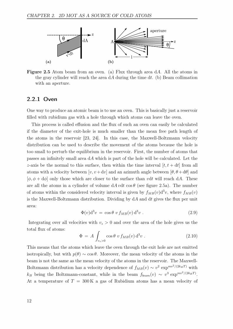
Our setup consists of an optical table with the laser setup and the 2D MOT itself

which can be connected to the main chamber on a CF16 flange. The 2D MOT has a

very modular and compact design which consists of a glass cell which is connected to

an optics module via a midpiece. The optics module can easily be seperated from the

rest of the setup.

In the first subsection the laser system with the beam paths for the 2D MOT will

be covered and in the second subsection a detailed description of the 2D MOT setup

will be given.

(a) (b)

Figure 3.1 Picture of the setup. (a) All the optics is placed on a solid cage thatsurrounds a glass cell with rubidium dispensers. (b) Picture of the optical table.

3.1 Laser system

To operate the 2D MOT, two lasers are necessary which are stabilized at different

hyperfine transitions of the trapped atoms. In the experiment 85Rb is used which

has a nuclear spin of I = 5. Due to hyperfine coupling, the ground state 52S1/2

splits up into two sub-states F = 2, 3, the excited state 52P3/2 splits up into four

23

CHAPTER 3. REALIZATION OF THE 2D MOT

Figure 3.2 Hyperfine level scheme of Rb with cooling scheme for 2D MOT. Thecooling laser is red detuned from the F = 3 → F ′ = 4 transition. The repumperpumps the atoms that fall into the dark state back into the cooling cycle. Theprobe beam is resonant with the F = 3 → F ′ = 4 transition.

substates F = 1, 2, 3, 4. The energy splittings of the hyperfine substates of the D2

line 52S1/2 → 52P3/2 used for cooling of the rubidium atoms are shown in figure 3.2.

In order to cool the atoms a cooling and a repumping laser are needed. The cooling

laser drives the F = 3 → F ′ = 4 closed cooling transition, but since the energy splitting

of the F ′ = 3 and F ′ = 4 sub-states is only 121MHz some of the atoms will unavoidably

be pumped into the F ′ = 3 state. From there they can decay spontaneously into the

F = 2 ground state which cannot be addressed by the cooling laser and is therefore a

dark state. This happens approximately once every thousand cooling cycles. Therefore

we need a repumping laser that pumps the atoms from the F = 2 dark state back into

the cooling cycle. To operate the 2D MOT and to characterize the atom beam, we

need three different laser beams:

• For the cooling beams we need light that is red detuned from the F = 3 → F ′ = 4

cooling transition and resonant light on the F = 2 → F ′ = 3 transition to pump

back the atoms that fall into the dark state.

• An enhancement of the normal 2D MOT is the so called 2D+ MOT [6] where

an additional pair of laser beam is put in the direction of the atom beam. These

beams are also red detuned from the F = 3 → F ′ = 4 transition and can be

used to modify the velocity distribution of the atoms.

• Finally, to characterize the atom beam, we need a probe beam with resonant

light on the cooling as well as the repumping transition (see section 4.1).

24

3.1. LASER SYSTEM

Figure 3.3 Locking scheme of the cooling laser. The TA is locked on the F’=3/4crossover, but it runs on the F’=2 transition due to the AOM before of the spec-troscopy. The cooler, pusher and probe beam are then shifted seperately by doublepass AOM’s to their desired frequencies.

3.1.1 Cooling laser

The cooling laser is a Toptica TA Pro. This laser is based on a diode laser (DL Pro)

that is coupled into a tapered amplifier chip. The beam is amplified in a single pass

through the chip preserving the spectral properties of the beam and then coupled into

a single mode fiber. The tapered amplifier chip makes it possible to reach output

powers as high as 1.3W (730mW after the fiber) which would destroy the facet of a

normal laser diode. In order to protect the diode laser from retro reflected light a 60dB

optical isolator is placed between the DL Pro and the TA chip. Between the isolator

and the tapered amplifier, a test beam is split off that is used for the spectroscopy to

stabilize the laser frequency.

The laser is mounted on an optical table that also contains the beam paths for the 2D

MOT. Only the spectroscopy is placed on a separate breadboard that is placed under

the optical table and set on a Sorbothane sheet to damp vibrations. The test beam

is transfered to the spectroscopy in a single mode polarization maintaining fiber. On

the spectroscopy board (figure 3.4), the beam first passes an acousto-optical modular

(Crystal Technology 3000 Series) that is set up in a double pass configuration and

shifts the laser frequency by 2 × 62MHz. Afterwards the beam is split up, one part

passes an 1 : 3 telescope and is send through a Rubidium vapor cell to be used for

Doppler free saturation spectroscopy. The other part is coupled into a Fabry Perot

interferometer to exhibit the mode profile of the laser. Using FM spectroscopy, the

laser is locked on the F ′ = 3/4 crossover which provides the largest signal. This means

that the laser is running on the F = 3 → F ′ = 2 transition (figure 3.3).

On the optical table (figure 3.5), the beam is split up into cooling, pushing and probe

25


Figure 3.4 Doppler free spectroscopy for laser lock. The Doppler free spectroscopyboard includes two spectroscopy branches to lock both lasers. Both lasers are alsocoupled into a Fabry Perot interferometer and can be shifted in frequency by anAOM in double pass configuration.

Figure 3.5 Beam Paths for the 2D MOT. All beams are shifted in frequency usingAOMs. Afterwards the beams are coupled into fibers to transfer them to the 2DMOT setup.

26

3.1. LASER SYSTEM

Figure 3.6 Locking scheme of the repumper. The diode laser is locked on the F’=2/3crossover, but it runs 142MHz higher due to the AOM before of the spectroscopy.The repumper beam is then shifted by a single pass AOM to the F’=3 transition.

beam by polarizing beam splitters (PBS) in combination with half-wave plates. All

beams are shifted to their desired frequencies with acousto-optic modulators (AOM).

Thereby the detuning of the cooler and pusher beams can easily be optimized by

changing the AOM frequencies. In a single pass configuration of the AOM, this would

cause the beam position to shift when changing the AOM’s frequency. Since all beams

are coupled into fibers to transfer them to the 2D MOT, this would cause intensity

fluctuations as already a small shift of the beam position significantly decreases the

coupling efficiency. Therefore, all the beams apart from the repumper are set up in

a double pass configuration [35] where the beam passes the AOM twice. Thus the

frequency can be adjusted without any significant changes in the beam position. A

disadvantage of passing the AOM twice is that we loose about 15−20% of laser power

every time the beam passes the AOM. After passing the AOMs, all the beams are

coupled into optical fibers.

3.1.2 Repumping laser

The repumper is a home build diode laser in Littrow configuration [36]. For a detailed

description of the diode laser setup see [37]. The laser beam passes an optical isolator

to protect the diode laser from back reflections. Then a small fraction of the light is

split off to be used for the FM spectroscopy which is identical to the one of the cooling

laser. The beam is shifted by 2 × −71MHz before being send to the spectroscopy

where it is locked on the F ′ = 2/3 crossover.

On the optical table, the beam is split up into two beams both of which are shifted

by 110MHz to be on resonance to the F = 2 → F ′ = 3 transition. One beam is then

superimposed on the cooling beam using a PBS which leads to a crossed polarization

of the two beams. The other beam is superimposed with the probe beam.

27


3.1.3 Laser cubes

Before the light is transfered to the 2D MOT setup, the trapping beam, as well as

the pusher beam are divided into two beams. This is done using Schäfter+Kirchhoff

laser cubes. In these cubes, the trapping beam is coupled out of the fiber and equally

split up into two beams. Since the two beams are coupled into the fiber with crossed

polarizations this can be done with a polarizing beam splitter in combination with

an adjustable half-wave plate. Also a small fraction (about 1%) is split off the beam

using a glass plate and then detected on a photodiode. This can be used to monitor

the laser power in the beam which is particularly useful when coupling the beam into

the fiber on the optical table. At the end all four beams are coupled back into four 15

meter long polarization maintaining fibers, to transport the light to the 2D MOT.

3.2 2D MOT setup

Figure 3.7 Design of the 2D MOT. A cage with all the optics is placed around theglass cell which is filled with rubidium gas.

Our 2D MOT consists of a glass cell that is surrounded by a metal cage holding

all the optics for three cooling regions and the pusher beams (figure 3.7). The glass

28

3.2. 2D MOT SETUP

Figure 3.8 Center piece of the 2D MOT setup. The center piece connects all thedifferent components of the 2D MOT.

cell provides perfect optical access from all directions and is filled with rubidium from

dispensers.

The 2D MOT was designed to be as modular and compact as possible and ensure a

high flux of cold atoms in order to load a 3D MOT as fast as possible. The complete

2D MOT setup has a size of 20 × 20 × 40 cm and can be mounted onto the main

chamber in one piece. The only connections needed are four optical fibers for the

different laser beams and electrical connections for the compensation coils and the

dispensers. The center piece of our design is a 82 × 74 × 24mm stainless steel part

(figure 3.8), that connects all the different components of the setup. On one side, a

bellow is connected on a CF40 flange to mount the setup on the UHV chamber. On

the other side, another CF40 flange connects the mid piece with the glass cell. To the

sides of the mid piece, there are two CF16 flanges, that are equipped with electrical

feedthroughs to connect the dispensers. Also on the sides, one finds several threaded

holes where the cage with the optics can be mounted. In the following, the different

components will be discussed in more detail.

3.2.1 Bellow with differential pumping tube

The bellow mounts the 2D MOT on the main vacuum chamber and is closed on its

CF40 side. The only connection between the two chambers is a 13 cm long differential

pumping tube with an inner diameter of 8mm which has an 800µm hole on the 2D

MOT side. It enables us to keep the rubidium pressure in the glass cell at around

10−7mbar, whereas the pressure in the main chamber should be 10−10mbar or less.

The end of the tube is polished and tilted by 45°, serving as a mirror for a counter-

propagating pusher beam.

29


Figure 3.9 Alignment of the differential pumping tube. Once the horizontal laserbeam is reflected horizontally again, the adjustment is complete.

The pumping tube is directly screwed into the bellow and fixed with a counter-

screw. Since the position cannot be changed after assembly, it is important that the

polished surface is oriented towards the outcoupler of the pusher beam. To align the

tube, a horizontal laser beam and two irises are used (see figure 3.9).

Since the bellow is the only fixed connection between the 2D MOT and the rest of

the setup, it can be used to change the relative orientation of the 2D MOT to the main

chamber. This is done with three threaded rods that are connected to the bellow on

one side. On the other side, three threaded tubes are placed in recesses so they can

be rotated and screwed onto the rods which then works like three telescope bars. This

allows us to fine adjust the atom beam for optimal loading of the three dimensional

trap.

3.2.2 Glascell

Figure 3.10 Technical drawing of the glass cell (Japan Cells).

The glass cell (figure 3.10) is made form Schott Tempax Borofloat glass with an AR

coating for 780nm on the outside of the cell. We decided to leave the inside of the cell

uncoated because the coating can act as a getter material for rubidium, which could

create a metal mirror on the surface of the cell. Some groups successfully use coatings

30

3.2. 2D MOT SETUP

Figure 3.11 Connection of the dispensers. The dispensers are connected to thefeedthrough with barrel connectors and sit to the side of the differential pumpingtube.

on the inside of the cell, but we did not want to take any chances. Our cell provides

us with 140mm of coated glass (figure 3.10), which is enough for three cooling regions,

each of which taking up about 35mm. Inside the glass cell up to four dispensers

contain the necessary rubidium. Two electrical feedthroughs that are placed on CF16

flanges on the sides of the mid piece provide the electrical connection to the outside

of the vacuum. The wires of the feedthroughs are bend at 90° so that the ends point

towards the rear side of the glass cell. The dispensers are directly connected to the

feedthrough using barrel-connectors (figure 3.11). The dispensers we used (Alvatec

AS-3-Rb-20-F), contain 20mg of rubidium in a cylinder shaped canister that is sealed

with indium. To open the dispensers, there is a special procedure [38] which includes

several steps at different currents, in order to break the seal and start the emission

of rubidium vapor. The activation is preferably done during a bake out, but can also

be done under normal vacuum conditions. After activation, the dispensers produce a

directed jet of rubidium vapor, in our case pointing to the far side of the glass cell.

The rubidium pressure can be controlled by changing the current of the dispensers.

3.2.3 Optics

All the laser light is transfered from the optical table to the 2D MOT via polarization

maintaining single mode fibers. At the 2D MOT, the fiber outcouplers are placed

in matched fittings, that form a bow over the outcoupler and are open on one side

(figure 3.12). At this opening a M4 screw is used to slightly compress the holder, just

enough to lock the outcoupler into position. The holder is connected to the mid-piece

by two screws and two positioning pins. Those pins allow for removal of the entire

31


Figure 3.12 Holder for fiber outcouplers. The holder is positioned using two pins andthen fixed by two screws. This way the fiber coupler can be removed withoutlosing the beam alignment.

holder without risking a misalignment of the beam. This was tested using a position

sensitive detector (Thorlabs PDQ 90S1) to measure the position of the outcoupled

beam after removing the entire holder numerous times from the mid piece. During

this measurement, the position of the beam varied by less then 0.1%. The same result

was obtained when only removing the outcoupler from the fitting. The outcouplers for

the two cooling/repumping fibers produce elliptical beams with a long axis of 22mm

and a short axis of 11mm (1/e2 values). Both beams are then split up into three

beams by a sequence of two polarizing beam splitters. All optics is placed as compact

as possible, in order to move the three cooling regions as close together as possible.

This is done using cube shaped modules (figure 3.13) that have a PBS in the middle

and are mounted onto mirror holders. The wave plates are glued into copper rings

that are placed into special fittings on the faces of the cube which are open at the top.

This way, the copper rings containing the quarter- and half-wave plates can still be

rotated after the faces of the cube are enclosed with two aluminium plates, to prevent

the rings from falling out of the fitting. The rings containing the wave plates can be

fixed in their final positions with M2 set screws. The power distribution among these

three beams can be controlled with half-wave plates, that are placed in front of every

PBS. Every beam also passes through a quarter-wave plate to achieve the circular

polarization needed for the trapping of the rubidium atoms. Then the beams pass the

glass cell and are retro-reflected by a mirror placed behind another quarter-wave plate

(figure 3.14). All three cooling regions add up to a total MOT length of up to 66mm.

The elliptical profile of the beams was chosen to ensure saturation of the cooling

transition, all over the cooling region. The two pushing beams have a diameter of

32

3.3. MAGNETIC FIELD DESIGN

8mm and are aligned to the center line of the glass cell. As mentioned above, the front

face of the differential pumping tube serves as a mirror for the counter-propagating

pusher beam. The next section deals with the magnetic field setup that is also part

of the cage with all the optics.

Figure 3.13 Splitting of the trapping beam. These compact optics modules are usedto split up the beam for the three cooling regions and to polarize all beamscircularly.

Figure 3.14 Optics module with glass cell in the center (top view)

3.3 Magnetic field design

For cooling of the rubidium atoms in two dimensions, a magnetic field gradient of

about 15G/cm is needed along these two directions and no field component in z-

33


direction. Most commonly, this field is produced by quadrupole coils. We decided to

use permanent magnets instead (figure 3.14).

Figure 3.15 Optics module with glass cell in the middle (side view). In a plane witha 45° angle to the laser beams sit the magnets.

3.3.1 Permanent magnets

Permanent magnets are made from materials with a magnetic dipole moment on mi-

croscopic scale. Usually these moments are orientated randomly averaging out any

magnetic moment on macroscopic scale. In a permanent magnet all the magnetic

dipole moments are aligned which can create quite strong fields on a macroscopic

scale as well. The permanent magnets we used are 25 × 3 × 10mm bars made from

neodymium (RS Components No.434-6877). The axis connecting the magnetic north

and south pole coincides with the short axis (3mm long) of the magnet. This axis

will be denoted as the y-axis in the following. The magnetic field of a cubical shaped

magnet like ours is given by [39]:

Bx(x, y, z) = −µ0M

4π

1∑

i,j,k=0

(−1)i+j+k arcsinh

(

z − zk√

(x− xi)2 + (y − yj)2

)

By(x, y, z) = +µ0M

4π

1∑

i,j,k=0

(−1)i+j+k arctan

(

(x− xi)2(z − zk)

2/(y − yj)2

√

(x− xi)2 + (y − yj)2 + (z − zk)2

)

Bz(x, y, z) = −µ0M

4π

1∑

i,j,k=0

(−1)i+j+k arcsinh

(

x− xk√

(z − zi)2 + (y − yj)2

)

(3.1)

Here Bx, By and Bz are the three Cartesian components of the magnetic field, µ0 =

4π×10−7Vs/Am is the magnetic constant, M is the magnetization which is a material

specific parameter with unit A/m. Finally (x0, y0, z0) = ~rmin and (x1, y1, z1) = ~rmax

34


are two opposite corners of the magnet, that define its spatial position.

3.3.2 Magnetization

Figure 3.16 Measurement of the magnetization of a permanent magnet. Measure-ment a is taken at the center of the magnet, measurement b along the side ofthe magnet.

To determine the magnetization of the permanent magnets, the magnetic field along

the axis at the center of the magnet was measured using a hall probe (SMT Teslamter

907) mounted on a three dimensional translation stage (figure 3.16). This measurement

would have been enough to determine the magnetization. In this case the data could

have been fitted by taking the magnetization and a relative z offset between translation

stage and magnet as fitting parameters. But it turned out that the accuracy could be

increased by taking a second measurement with an offset in x-direction (in our case

x = 1.26 cm) to determine the relative z offset separately. This result is then used

to fit the data of the first measurement with the magnetization being the only fitting

parameter (figure 3.17). The increase in accuracy when taking two measurements is

due to the fact, that the second measurement is more sensitive for the the relative

z position towards the magnet, since the field over a much longer distance could be

measured on both sides of the magnet. The Hall probe over-saturated when getting

too close to the magnet on the center line. The final result was a magnetization of

M = (8.7± 0.2)× 109A/m .

The limiting factor for the accuracy of the measurement was the error of the Hall

probe signal and the relative positioning of magnet and translation-stage. Also the

deviation of the magnetization for different magnets was measured. The measurement

was carried out by putting the magnets in a special fitting, the size of a magnet

and placing the hall probe above the center of the magnet. Now we could place

different magnets in the holder, ensuring that the distance between the magnets and

35


(a) (b)

Figure 3.17 Magnetic field of the permanent magnet. (a) Fit of the magnetic fieldwith the hall probe moving along the center line of the magnet and (b) with adisplacement of x = 1.26 cm to the side

the hall probe was always the same. The measurement shows (table 3.1), that the

magnetization of the magnets varies by approximately 3%. Now we have completely

characterized the magnets and can combine the fields of several magnets to create a

two dimensional quadrupole field.

Table 3.1 Magnetization of different magnets. The magnetization of the permanentmagnets varies by approximately 3%.

Number Magnetic field (G) Magnetic field (G)magnet front side rear side

1 40 -39.42 39.3 -38.73 38.5 -39.74 39 -39.75 39.3 -39.26 40.2 -39.5

3.3.3 Setup of the magnets

In the following there are two different coordinate systems we are going to use, one

being the system of the magnets and the other one being the system of the glass cell

and the lasers. The system of the lasers is going to be denoted ~r′ = (x′, y′, z′), the

system of the magnets will be denoted ~r = (x, y, z). The z axes of both systems are

36


Figure 3.18 Design of the magnet holder. On both sides of the glass cell, an arrayof six permanent magnets (blue) is mounted onto a holder. The position of themagnets was optimized to get a smooth magnetic field gradient. Therefore, themagnets in the middle are moved further to the back. On both sides the fifthmagnet is placed on a translation stage. This way the zero line of the magneticfield can be shifted at the position of the exit hole.

the same, being the symmetry axes of the two rows of magnets, as well as the center

line of the glass cell. For our 2D MOT we use two rows of six magnets each. The

magnets are glued onto a holder that is placed under a 45° angle with respect to the

faces of the glass cell (figure 3.18). To calculate the magnetic field of this setup, one

has to add the magnetic field (equation (3.1)) of all twelve magnets

~Btotal =

12∑

n=1

~Bn , (3.2)

Bn being the field of the nth magnet. The magnetic field of all twelve magnets is

shown in figure 3.19 and figure 3.20. Note that the dipole moments of the magnets in

the upper row are oriented in the opposite direction to the magnets in the lower row.

This means that the magnetic field of both cancel each other at the center. One gets

an almost perfect two-dimensional quadrupole field with the zero line of the magnetic

field along the center of the glass cell. On a length of about 8 cm on the two axes

coinciding with the cooling beams, the gradient is almost constant. In order to get the

same gradient at all positions of the z axis too, the inner magnets have to be moved

further away from the glass cell. The reason is, that in the middle, the field of the

neighboring magnets adds up, which leads to a steeper gradient in the center then at

the sides. The position of the magnets was optimized for a field gradient of 15G/cm.

37


(a) (b)

Figure 3.19 (a) Vector field of the permanent magnets in the z=0 plane. (b) Zoominto the center of the field where the atoms are trapped.

Other gradients can also be obtained by moving the magnet holders to a different

position in the x′-direction. The holder can be moved to five different positions where

it is fixed with special positioning screws. The five accessible gradients are 10.6,

12.6, 15.2, 18.5 and 23.0G/cm. To position the magnets on the holder a template

with a pit at the position of each magnet is used. The magnets are glued into these

pits with two-component adhesive (Uhu endfest 300). After the glue hardens within

a day, the template is left in position because it adds some extra stability to the

magnets. To see how good the magnetic field matched the calculations, the field of

one configuration was measured with a three dimensional hall probe. The result is

shown in figure 3.16. There is a slight deviation of the magnetic field gradient from

the calculations on the right side. But this error is within the range of the fluctuations

of the magnets’ magnetization mentioned earlier. These small fluctuations are not

very important concerning the slight change of the gradient, since this is not a very

sensitive parameter for capturing the atoms, at least on this scale. But it is critical

when it comes to the zero line of the magnetic field. The trapped atoms are going

to follow that zero line and already a small offset can cause the atom beam to miss

the 800µm exit hole in the differential pumping tube. Already the earths magnetic

field (about 400mG in Heidelberg) causes a shift of about 270µm at the 15G/cm

configuration. Another error source is the position of the magnets. Therefore the last

but one magnet was placed on a small translation stage. Moving this magnet changes

the magnetic field at the end of the last cooling region before the atoms head towards

the exit hole. The idea is that with this degree of freedom the atom beam could be

38


Figure 3.20 Magnetic field gradient in the plane of the laser beams. On the left acontour plot of the magnetic field in the plane of the laser beams is shown. Onthe right side B(z′) along the x′ = 0 axis is shown. The obtained gradient isclose to constant for −5 < z′ < 5 and −8 < z′ < 8.

4

6

8

10

12

14

-10 -5 0 5 10

field

gra

die

nt∇B

(G/cm)

z position (cm)

calculationmeasured points

Figure 3.21 Magnetic field gradient. Every point shown in the graph consists of fivedata points that were taken at different x-positions and then used to fit thegradient at that point. The solid line shows the calculated curve.

39


coupled into the pumping tube.

The experiment showed that only one degree of freedom is not enough to accomplish

that. In order to adjust the beam through the hole it is necessary to have full control

over the magnetic field in both x- and y-direction. It would be beneficial to move

the whole holder with all magnets rather than only bending the field at the last

cooling region, because the straighter the zero line of the magnetic field, the easier

the atoms can follow the field. To get both degrees of freedom needed two pairs of

compensation coils in x′- and y′-direction were installed which add a constant field

along their symmetry axis thus shifting the zero line in that direction. Now the atom

beam can be moved in two dimensions in order to pass through the differential pumping

tube. To see how critical the alignment of the magnetic field really is the atom flux

behind the pumping tube as a function of the compensation field was measured (see

section 4.5.2).

40

4 Characterization of the atom

beam

Before connecting the 2D MOT to the main vacuum chamber it is optimized on a test

chamber. Good optical access enables us to take time of flight measurements with a

sensitive photodiode. This way the atom beam could fully be characterized and the

flux could be optimized for our later requirements. The velocity distribution of the

beam is particularly interesting in order to load the 3D MOT because only atoms

under a certain capture velocity can be captured.

In the first section details of the test setup are shown and the way different pa-

rameters were measured is explained. Afterwards the results of the measurements are

presented. This includes the measurement of the velocity distribution and the total

flux as a function of the various parameters that are accessible in our setup. For all

measurements only one parameter was changed and all the other settings were put on

their optimum values. The results will also be compared to results from our simula-

tion and other experiments. Table 4.1 gives on overview of the beam characteristics

of different rubidium atom sources.

experiment mean beam total flux luminosityvelocity (m/s) divergence (mrad) (s−1) (atoms s−1 rad−1)

Dieckmann [6] 15 43 5× 109 3.4× 1012

Dieckmann [6] 8 43 9× 109 6.2× 1012

Schoser [7] 60 32 5× 1010 6.2× 1013

Wohlleben [28] 14 10 1× 108 1.3× 1012

Utfeld [40] - 30 3× 108 4.2× 1011

our result 14 26 4× 109 7.5× 1012

Table 4.1 Beam charcteristics of other Rb 2D MOTs.

4.1 Test setup

In order to characterize the atom beam, the 2D MOT is flanged onto a test chamber

(figure 4.1) that consists of two CF40 six-way crosses and one four-way cross. The

41

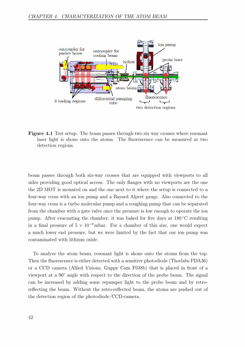
CHAPTER 4. CHARACTERIZATION OF THE ATOM BEAM

two detection regions

Figure 4.1 Test setup. The beam passes through two six way crosses where resonantlaser light is shone onto the atoms. The fluorescence can be measured at twodetection regions.

beam passes through both six-way crosses that are equipped with viewports to all

sides providing good optical access. The only flanges with no viewports are the one

the 2D MOT is mounted on and the one next to it where the setup is connected to a

four-way cross with an ion pump and a Bayard Alpert gauge. Also connected to the

four-way cross is a turbo molecular pump and a roughing pump that can be separated

from the chamber with a gate valve once the pressure is low enough to operate the ion

pump. After evacuating the chamber, it was baked for five days at 180 C resulting

in a final pressure of 5 × 10−8mbar. For a chamber of this size, one would expect

a much lower end pressure, but we were limited by the fact that our ion pump was

contaminated with lithium oxide.

To analyze the atom beam, resonant light is shone onto the atoms from the top.

Then the fluorescence is either detected with a sensitive photodiode (Thorlabs PDA36)

or a CCD camera (Allied Visions, Guppy Cam F038b) that is placed in front of a

viewport at a 90° angle with respect to the direction of the probe beam. The signal

can be increased by adding some repumper light to the probe beam and by retro-

reflecting the beam. Without the retro-reflected beam, the atoms are pushed out of

the detection region of the photodiode/CCD-camera.

42

4.1. TEST SETUP

-0.3

-0.28

-0.26

-0.24

-0.22

-0.2

-0.18

0 0.01 0.02 0.03 0.04

PD

sig

nal(V

)

time v (s)

(a)

10 20 30 40

0

0.1

0.2

0.3

ato

mflux

velocity v (m/s)

(b)

Figure 4.2 Measurement of the velocity distribution. (a) Fluorescence signal on thephotodiode. At t = 0 the cooling laser was switched to a blue detuning (−8MHz)in order to stop the atom flow. The velocity distribution (b) is obtained bydifferentiating the fluorescence signal.

4.1.1 Measurement of the velocity distribution

The velocity of the atoms is especially important for the loading efficiency of the 3D

MOT. Typical capture velocities vcap are in the range of 25-40m/s. This is why we

are not only interested in the total flux of atoms, but also in the velocity distribution

of the beam. In particular the flux of atoms below the capture velocity Φ(v < vcap).

For this measurement, the sensitive photodiode was used at the first detection region

in order to get a time resolved fluorescence signal. To collect light from a bigger solid

angle, a combination of three plano-cenvex lenses (two inch) was placed in front of the

photodiode. First a f = 100mm lens with the atom beam sitting in the focus of the

lense collects the light, followed by two f = 60mm lenses to focus the light onto the

photodiode. Two f = 60mm lenses are used because lenses with a smaller focal length

are not available with a two inch diameter. The lenses were placed in a lens-tube with

an iris and the photodiode placed at the end of the tube to minimize the background

signal from stray light.

To take time-of-flight measurements, the beam has to be switched on and off. In

order to prevent systematic errors this has to be done at an exactly known location.

Simply blocking the cooling beam for instance does not produce a good signal as all

atoms that are already trapped could still exit the hole. Switching the cooling beams

to a blue detuning blows away already trapped atoms, thus effectively cutting of the

beam at the end of the last cooling region in front of the exit hole. This is done by

43


switching the AOM for the cooling beams between the normal detuning of δ = 12MHz

to a blue detuning of δ = −8MHz.

The atom beam is switched off at t = 0. It takes an atom ∆t = d/v to reach

the detection region, d being the distance to the probe beam and v being the atoms

longitudinal velocity. For t < d/v atoms with a velocity of v still fly through the

detection region. At time t = d/v the last atoms with velocity v enter the detection

region and the flux stops. For all times t > d/v this velocity class is missing from the

photodiode signal. This means that the signal U(t) is proportional to the fluorescence

of all atoms with 0 < v < d/t:

U(t) ∼∫ v=d/t

v=0

N(v′)dv′ .

N(v) is the atom-distribution and d is the distance from the 2D MOT to the detection

region. Substitution of t′ = d/v′ leads to

U(t) ∼∫ t=d/v

t=∞

N(d/t′)d

t′2dt′

⇒ ddt

U(t) ∼ ddt

∫ t=d/v

t=∞

N(d/t′)d

t′2dt′ = N(v)

v2

d

⇒ N(v) ∼ d

v2dUdt

.

The atom-flux-distribution is Φ(v) = N(v)× v. This gives us

Φ(v) = ξd

v

dUdt

(4.1)

The proportionality factor ξ converts the signal of the photodiode U(t) into the

number of atoms in the detection region. Note that there is a difference between

the number of atoms in the detection region and the atom distribution N(v). The

atom-distribution already accounts for the fact that slow atoms scatter more photons

because they need longer times to pass the detection region.

The atoms scatter light with Γ2= 1

τwhere Γ = 6× 2 πMHz is the natural linewidth

of the F = 3 → F ′ = 4 transition with a lifetime of τ = 27 ns. But we only detect

the light in the solid angle of the lenses placed in front of the photodiode. With a two

inch lens at a distance of 10 cm we get a solid angle of Ωpd = 1.6%. We also have to

take into account that the viewports are not coated and we loose approximately 10%

of power on both surfaces of the glass. The quantum efficiency of the photodiode was

44

4.1. TEST SETUP

measured with a laser by measuring the voltage drop as a function of the laser power.

This gave us a ratio of κ = 1.0 × 106V/W. Taking everything into account we get a

proportionality factor of

ξ = 0.81 κΓ

2Ωpd hν dprobe

Here h is Planck’s constant, ν is the frequency of the atomic transition and dprobe is the

width of the probe beam which is the length of the detection region. Now we can use

equation 4.1.1 to calculate the velocity distribution from the signal of the photodiode

(figure 4.2b). In order to minimize noise the photodiode signal was averaged over 16

measurements.

4.1.2 Measurement of the flux

To calculate the total flux of atoms, the atom-flux-distribution can be used. The

height of the fluorescence signal is not a good indicator for the total flux. As mentioned

before, the number of photons a single atom scatters is proportional to its longitudinal

velocity. This means a slow atom beam would result in a much higher fluorescence

signal than a fast atom beam. This is why we need the velocity distribution of the

beam to put a number on the total flux.

The total atom flux simply is the integral over the atom-flux-distribution:

Φtot =

∫

∞

0

Φ(v) dv

For our experiment an even better benchmark is the flux of atoms with velocities below

the capture velocity of the 3D MOT:

Φcap =

∫ vcap

0

Φ(v) dv

The area under the curve was calculated by using a box integral.

Measuring the flux by taking the velocity distribution some systematic errors occur:

• In the calculation we assumed that all atoms scattered into the solid angle of the

lense in front of the photodiode are detected. Due to misalignment of the imaging

lenses it is likely that we loose a good portion of those photons because they miss

the detecting area of the photodiode. This means that we underestimate the flux.

• The opposite effect occurs as photons are also scattered into the detection angle

from the walls of the chamber. We only want to detect atoms that are comming

directly from the atom beam but some of the photons that are scattered in

another directions might be reflected back onto the photodiode.

45


• We also assumed that we detect all the atoms that are within the detection

region of length dprobe. But since the diameter of the probe beam is smaller than

the width of the atom beam at the first detection region, we only illuminate the

center of the beam.

With some effort, it would be possible to further diminish the systematical errors just

mentioned, but the most reliable result would still be obtained by using the beam to

load a three dimensional MOT and to measure the loading curve. For the results in

the following section this means that the total atom flux shown in the graphs has a

quite large systematical error. This error should be the same for all measurements

taken and the error bars shown in the graphs only relate to the statistical error due

to fluctuations during the measurements.

4.2 Beam divergence

(a) (b)

Figure 4.3 (a) Atom beam on the CCD camera. The atom beam was made visiblewith a 6mm probe beam and then detected with a CCD camera at a 90 angle. (b)CCD image of a template with 0.5mm lines that we used to calibrate the camera.

The divergence of the atom beam is a very important parameter. It tells us how big

the beam is going be at the position of our 3D MOT which can be compared to the

size of the capture region of the trap. If the area, where we can effectively trap the

atoms is smaller than the atom beam, atoms are lost.

There is an upper limit for the divergence of the atom beam that is set by the

geometry of the differential pumping tube (figure 4.4). For the dimensions of our

tube, this limit is αmax = 64mrad. To measure the divergence of the atom beam an

image of the beam is taken with the CCD-camera. The camera’s exposure time is

40ms and an Lab-View interface is used to read out the charge state of every pixel

on the camera. To measure the divergence, the exact distance to the exit hole of the

46

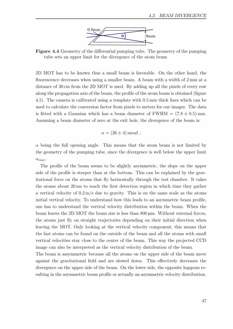
4.2. BEAM DIVERGENCE

Figure 4.4 Geometry of the differential pumping tube. The geometry of the pumpingtube sets an upper limit for the divergence of the atom beam

2D MOT has to be known thus a small beam is favorable. On the other hand, the

fluorescence decreases when using a smaller beam. A beam with a width of 2mm at a

distance of 30 cm from the 2D MOT is used. By adding up all the pixels of every row

along the propagation axis of the beam, the profile of the atom beam is obtained (figure

4.5). The camera is calibrated using a template with 0.5mm thick lines which can be

used to calculate the conversion factor from pixels to meters for our images. The data

is fitted with a Gaussian which has a beam diameter of FWHM = (7.8 ± 0.5)mm.

Assuming a beam diameter of zero at the exit hole, the divergence of the beam is:

α = (26± 4)mrad ,

α being the full opening angle. This means that the atom beam is not limited by

the geometry of the pumping tube, since the divergence is well below the upper limit

αmax.

The profile of the beam seems to be slightly asymmetric, the slope on the upper

side of the profile is steeper than at the bottom. This can be explained by the grav-

itational force on the atoms that fly horizontally through the test chamber. It takes

the atoms about 20ms to reach the first detection region in which time they gather

a vertical velocity of 0.2m/s due to gravity. This is on the same scale as the atoms

initial vertical velocity. To understand how this leads to an asymmetric beam profile,

one has to understand the vertical velocity distribution within the beam. When the

beam leaves the 2D MOT the beam size is less than 800µm. Without external forces,

the atoms just fly on straight trajectories depending on their initial direction when

leaving the MOT. Only looking at the vertical velocity component, this means that

the fast atoms can be found on the outside of the beam and all the atoms with small

vertical velocities stay close to the center of the beam. This way the projected CCD

image can also be interpreted as the vertical velocity distribution of the beam.

The beam is assymmetric because all the atoms on the upper side of the beam move

against the gravitational field and are slowed down. This effectively decreases the

divergence on the upper side of the beam. On the lower side, the opposite happens re-

sulting in the asymmetric beam profile or actually an asymmetric velocity distribution.

47


0

0.1

0.2

0.3

0.4

0.5

0.6

0.7

0.8

0.9

1

0 2 4 6 8 10 12 14 16 18

norm

alize

dsi

gnalhig

ht

x (mm)

projection of the CCD imagegauss fit

Figure 4.5 Beam profile of the atom beam at the first view port. The profile wasobtained by projecting the CCD image. To make the atom beam visible we useda retro reflected probe beam with a diameter of 2mm.

4.3 Dependence on laser settings

In order to change the detuning and the power of the different beams the AOMs placed

in every beam path are used. Changing these two parameters is not fully decoupled.

When the frequency of the AOM is changed the diffraction efficiency changes as well

which results in a shift in beam power. Also the position of the beam changes leading to

a change in the coupling efficiency into the optical fiber. This effect was minimized by

setting up the AOMs in a double pass configuration but it can not fully be suppressed.

In order to change the detuning of the beams without changing its power the AOM

power was adjusted for every setting of the frequency as well.

4.3.1 Detuning cooling laser

The highest flux of atoms was measured for a detuning of δ = 12MHz = 2Γ (figure

4.6). In figure 4.6 also the results of our simulations (green triangles) is shown which

reproduce the measured data quiet nicely. To match the data, the fluxes from the

simulations are scaled down by a factor of two. The detuning of the cooler is an

important parameter for every magneto-optical trap:

• Together with the magnetic field gradient it defines the size of the trapping

48

4.3. DEPENDENCE ON LASER SETTINGS

volume. The smaller the detuning of the cooling laser, the smaller the volume

where the atoms are cooled.

• The detuning influences the shape of the trapping potential. For large detunings

we only get a weak confinement for the already trapped atoms.

Because of the smaller radius of the trapping volume at small detunings, the cooling

time of the atoms is strongly limited by their transverse velocity whereas their longi-

tudinal velocity is less critical. At higher detunings the longitudinal velocity becomes

the limiting factor of the cooling time leading to a reduction of fast atoms in the beam.

This can be seen in figure 4.7 where the number of fast atoms is larger for smaller

detunings.

4.3.2 Power cooling laser

For different powers of the cooling beams we see an almost linear increase of the flux

at low powers and a plateau at high beam powers (figure 4.8). At low powers the

scattering rate increases linearly with the laser power which leads to a higher capture

velocity and an increasing flux. As soon as the transition is saturated all over the

cooling volume and the scattering rate is close to its maximum of γ = Γ/2, the flux

levels out. For our setup with three cooling regions the plateau is reached at a power

of P ≈ 55mW in each of the two beams (x and y beam). This corresponds to a

saturation of I/I0 = 12 at the center of the cooling beams.

The simulation can reproduces the data quiet good again. The flux was scaled by

the same factor of two as in figure 4.6 to be comparable.

The peak velocity of the beam is slightly shifted to lower velocities with increasing

cooler power (figure 4.9). This is in contrast to the results in [7] where an increase

of the peak velocity at higher powers was observed. It was argued that since the

transverse cooling works more efficiently at high intensities, also atoms with higher

longitudinal velocity can participate in the beam. In [7] a conventional 2D MOT

without a pushing beam was used. In our case the peak in the velocity distribution is

mainly caused by atoms that first travel away from the exit hole and are then turned

around by the pushing beam (see section 4.3.4). This is a totally different situation

where the argument in [7] no longer holds.

Table 4.2 shows the cooler powers and detunings of other rubidium 2D MOTs. The

beam sources are divided into 2D MOTs (no pusher), 2D+ MOTs (with pusher) and

a MOT + pusher. The last one is a regular 3D MOT where the atoms are pushed

out by an additional laser beam. For a better comparability also the I/I0 value in the

49


0.5

1

1.5

2

2.5

3

3.5

2 4 6 8 10 12 14 16 18

ato

m-fl

uxΦ

(109

s−1)

detuning cooler δ (MHz)

Figure 4.6 The total atom flux as a function of the cooler’s detuning. The highestflux was observed for a detuning of δ = 12MHz. The green triangles show theresult of the simulation.

0

0.05

0.1

0.15

0.2

0.25

0.3

8 10 12 14 16 18 20 22 24

ato

m-fl

ux

dis

trib

uti

on

(r.u

.)

velocity v (m/s)

δ = 16MHzδ = 14MHzδ = 10MHzδ = 8MHz

Figure 4.7 Velocity distribution for different detunings of the cooler. The number offast atoms is increased at small detunings.

50


0.5

1

1.5

2

2.5

3

3.5

4

10 20 30 40 50 60 70 80 90

ato

m-fl

uxΦ

(109

s−1)

power cooler P (mW)

Figure 4.8 The total atom flux as a function of the cooler power. The atom fluxsaturates at a power of P ≈ 55mW. The green triangles show the result of thesimulation.

0

0.05

0.1

0.15

0.2

0.25

8 10 12 14 16 18 20 22 24

ato

m-fl

ux

dis

trib

uti

on

(r.u

.)

velocity v (m/s)

P = 23.4mWP = 29.0mWP = 42.6mWP = 62.0mW

Figure 4.9 Velocity distribution for different cooler powers. For higher cooling pow-ers, the peak in the velocity distribution is shifted to higher velocities.

51


center of the cooling beams is listed.

experiment beam total cooler detuning I/I0source power (mW) cooler (MHz)

Dieckmann [6] 2D MOT 16.4 10.2 7.8Dieckmann [6] 2D+ MOT 15 18 7.1

Schoser [7] 2D MOT 320 11.4 12.7Wohlleben [28] MOT + pusher 60 18 5.8

Fuchs [41] 2D+ MOT 35 10 5.6Utfeld [40] 2D+ MOT 150 7 10our result 2D+ MOT 110 12 12

Table 4.2 Laser settings of other Rb 2D MOTs. The total power is either the max-imum power available or the the power where the flux saturated. The saturationparameter I/I0 refers to the center of the cooling beam.

4.3.3 Repumping laser

The total atom flux also depends on the power of the repumper. Normally a few mW

of repumping power are sufficient since the atoms only fall into the F = 2 dark state

once every thousand cooling cycles. The repumping power was varied over a range of

1.5-3.5mW where the flux increased linearly with the repumping power (figure 4.10).

With the powers that were available during the time of the measurement no saturation

of the flux could be observed, so a further increase of the power should lead to a larger

flux. In [40] they had a similar setup and saw a saturation of the flux at a power of

P = 6mW.

The mean velocity of the beam is shifted to higher velocities with increasing re-

pumping power. The peak velocity is reduced by about 2m/s for a doubling of the

repumping power from 1.5mW to 3.1mW. This is quiet interesting since an increase

in the cooling power leads to lower velocities. To understand these dependences one

has to take a closer look at the pushing beam.

4.3.4 Pushing laser

In the 2D MOT two atom beams are produced, one in z and one in −z-direction. Due

to the symmetry of the setup there should be the same number of atoms traveling in

both directions. Without the pushing beam all the atoms traveling in −z direction

are lost. With a red detuned pushing beam on the axis of the atom beam it should be

possible to turn around some of the atoms traveling the “wrong” way. In this simple

52


1.6

1.8

2

2.2

2.4

2.6

2.8

3

3.2

3.4

3.6

1 1.5 2 2.5 3 3.5

ato

m-fl

uxΦ

(109

s−1)

power repumper P (mW)

Figure 4.10 The total atom flux as a function of the repumper power. The fluxincreases linearly with the power and there is no saturation of the flux withinthe measured range.

0

0.05

0.1

0.15

0.2

0.25

8 10 12 14 16 18 20 22 24

ato

m-fl

ux

dis

trib

uti

on

(r.u

.)

velocity v (m/s)

P = 1.5mWP = 2mW

P = 2.5mWP = 3.1mW

Figure 4.11 Velocity distribution for different repumper powers. For higher repump-ing powers the velocity distribution is shifted to lower velocities.

53


picture the maximum gain expected from the pushing beam would be a doubling of

the flux if all the atoms initially traveling in −z-direction can be turned around. This

is exactly what is observed in the experiment. Without the pushing beam we have

a total flux of Φ ≈ 1.9 atoms/s and with the pushing beam we can reach a flux of

Φ ≈ 3.7 atoms/s at a detuning of 40MHz and a power of 0.8mW (figure 4.12 and

4.13).

To get a qualitative understanding of the influence of the pushing beam, a simple

model will be used. The pushing beam can be described by the force in equation

(2.25) with B = 0 (there is no magnetic field component in z-direction). It has to be

considered that the pushing beam does not contain any repumping light. Therefore it

only acts on the atoms as long as they stay within the cooling volume of the 2D MOT

where they are pumped back from the dark state.

Figure 4.14 shows a phase space diagram of the atoms which are initially traveling

in −z-direction. Outside the cooling region of the 2D MOT the force is zero, therefore

the atoms travel with a constant velocityA. After the atoms enter the cooling region

they are slowed down by the pusher. The red trajectories represent atoms which pass

the cooling region before the pusher can stop them. The green trajectories represent

atoms which can be turned around by the pusher and are then accelerated back in z

direction. While the atoms get faster the force on them decreases because they are

further detuned from the pusher. This is why all green trajectories accumulate around

the same velocity where the atoms are out of resonance with the pushing beam.

To calculate the velocity distribution of the atoms after they are turned around,

their initial velocity distribution has to be known. The distribution should be the same

(with opposite signs) as the velocity distribution of the atoms traveling in z direction

(green curve in figure 4.15). The red curve shows a simulation of the atoms’ velocity

distribution after the pushing beam (with δ = 40MHz and P = 1mW) interacted

with the atoms. The simulation shows that most of the atoms change their direction

and pushed out of the cooling volume in z-direction. Only atoms which travel faster

than 50m/s (red trajectories in 4.14) leave the cooling region in −z-direction.

The blue line shows the measured velocity distribution with the pusher present.

The long tail of fast atoms can be interpreted as the atoms initially traveling in z

direction (green curve). The peak of the velocity distribution is roughly at 14m/s

which is reproduced quiet good in the simulation, whereas the width and hight are

different in the simulation. In the simulation all the atoms enter the cooling volume

at the same z value whereas they should start from points distributed all over the

cooling region. This could be accomplished by implementing the pushing beam into

the numerical simulation of the 2D MOT and should lead to a widening of the peak as

54


1.5

2

2.5

3

3.5

4

-20 -10 0 10 20 30 40 50 60

ato

m-fl

uxΦ

(109

s−1)

detuning pusher δ (MHz)

Figure 4.12 The total atom flux as a function of the pusher’s detuning. The highestflux is obtained at a detuning of δ = 40MHz.

1.6

1.8

2

2.2

2.4

2.6

2.8

3

3.2

3.4

3.6

0 0.5 1 1.5 2 2.5

ato

m-fl

uxΦ

(109

s−1)

power pusher P (mW)

Figure 4.13 The total atom flux as a function of the pusher power. Increasing thepusher power from 0mW (pusher off), to 1mW leads to a doubling of the totalflux.

55


Figure 4.14 Phasespace of atom beam with pusher. The phasespace of the atomsinitally travelling in the −z direction is shown. Red trajectories represent atomsthat are too fast to be turned around, green trajectories represent atoms thatare reflected by the pusher. Most of these trajectories accumulate around thesame final velocity. On the right the force F (v) on the atoms is shown.

in the measured curve. For an improved simulation the distribution of points where

the atoms enter the cooling volume has to be known. Nevertheless the simulation can

explain most of the measured dependences.

The velocity at which the atoms get out of resonance with the beam depends on

the pusher’s detuning and power:

• For higher powers the peak is shifted to higher velocities due to the power broad-

ening of the pushing beam.

• For larger detunings the peak is shifted to lower velocities.

This was also observed experimentally (see figures 4.17 and 4.16). For a detuning of

δ = 14MHz the peak is at a velocity of 11m/s. When increasing the detuning to

δ = 54MHz the peak’s velocity is shifted by about 50% to 11m/s. A change from

P = 0.5mW to 2.3mW in pushing power results in a shift of about 30% from 11m/s

to 15.5m/s.

As mentioned earlier, there is also a dependence of the peak position on the cooling

56


0

0.1

0.2

0.3

0.4

0.5

0.6

8 10 12 14 16 18 20 22 24

ato

m-fl

ux

dis

trib

uti

on

(r.u

.)

velocity v (m/s)

pusher onpusher offsimulation

Figure 4.15 Simulation of the pushing beam. The solid lines show the data takenwith (blue) and without (green) the pushing beam. The dashed line shows asimulation of the velocity distribution of the −z atom beam which is turnedaround by the pusher. The parameters used for the simulation are δpusher =40MHz and Ppusher = 1mW.

and repumping powers:

• The peak is shifted to lower velocities for larger cooling powers. The atoms

scatter more likely with the cooling laser the higher its power. Thus they scatter

less likely with the pushing beam which diminishes the force of the pusher.

• The peak is shifted to higher velocities for larger repumping powers because the

atoms are pumped back into the cooling cycle more efficiently. This increases

the force of the pusher.

The total flux of atoms that can be reached with the pushing beam depends on how

many atoms from the −z beam can be addressed by the pusher. In order to address a

lot of atoms it is favorable to have an atom beam with a narrow velocity distribution

to begin with. This can be illustrated by comparing the results by Dieckmann et al.

[6] and Schoser et al. [7].

The experiment performed by Dieckmann et al. produces an atom beam with a

width of the velocity distribution (FWHM) of about 25m/s at a mean velocity of

15m/s. They report an increase of the flux from 5 × 109 atoms/s without a pushing

beam, to 9× 109 atoms/s with a pushing beam. This is again close to a factor of two

as in our case.

57


0

0.05

0.1

0.15

0.2

0.25

0.3

0.35

10 15 20 25 30

ato

m-fl

ux

dis

trib

uti

on

(r.u

.)

velocity v (m/s)

δ = 54Hzδ = 40Hzδ = 32Hzδ = 14Hzδ = 0Hz

Figure 4.16 Velocity distribution for different detunings of the pusher. For biggerdetunings the peak in the velocity distribution is shifted to higher velocities.

0

0.05

0.1

0.15

0.2

0.25

0.3

8 10 12 14 16 18 20 22 24

ato

m-fl

ux

dis

trib

uti

on

(r.u

.)

velocity v (m/s)

P = 0.5mWP = 0.8mWP = 1.1mWP = 2.3mW

pusher off

Figure 4.17 Velocity distribution for different pusher powers. For higher pusher pow-ers the peak in the velocity distribution is shifted to higher velocities.

58


In the second experiment by Schoser et al. they have an atom beam with a width of

the velocity distribution (FWHM) of about 75m/s at a peak velocity of 50m/s. They

can only achieve a small increase of the flux by applying a pushing beam. Only the

slowest atoms of the atom beam can be adressed by the pusher since the width of the

velocity distribution is too large. It should also be mentioned that they used resonant

light for the pushing beam whereas our results suggest that it is beneficial to use far

red detuned light.

The last setting of the laser system that was investigated is the influence of a counter-

propagating pushing beam.

4.3.5 Counter-propagating pushing beam

A similar beam was used by Dieckmann et al. to shape the velocity distribution of the

atom beam. Without a significant change in the total flux they could lower the mean

velocity from 15m/s (without any pushing beams) to 8m/s, with the two counter-

propagating beams. The width of the velocity distribution dropped from 25m/s to

only 3.3m/s. The two beams had to be unbalanced to get the best result. More power

was used in the beam towards the exit hole.

Our measurement was taken for various power balancings at a number of different

powers and detunings. In all cases the flux was always better without the counter-

propagating pushing beam. Also in most cases the mean velocity of the beam was in-

creased rather than decreased. Figure 4.18 shows the velocity distribution for three set-

tings with the counter-propagating beam turned on and off. The counter-propagating

beam decreases the number of slow atoms. This might be interpreted as a reduction

of the others pushing beam’s efficiency.

The same effect was observed in [29] where they also saw a decrease in the number

of slow atoms due to the second pushing beam. Catani et al. [8], who investigated

a potassium 2D MOT, report a small decrease of about 20% in the mean velocity of

the beam.

In the experiment the detunings of the two pushing beams could not be adjusted

separately. It might be beneficial to detune the second pushing beam even further to

only address the fast atoms.

In the next two subsection the influence of the total MOT length, the pressure and

the magnetic field gradient will be discussed.

59


0

0.05

0.1

0.15

0.2

0.25

0.3

8 10 12 14 16 18 20 22 24

ato

m-fl

ux

dis

trib

uti

on

(r.u

.)

velocity v (m/s)

retro on δ = 44MHzretro on δ = 34MHzretro on δ = 24MHzretro off δ = 48MHzretro off δ = 34MHzretro off δ = 24MHz

Figure 4.18 Velocity distribution with/without a counter-propagating pushing beam.The solid lines show a setting where 820µW are in the pushing beam and 400µWin the counter-propagating beam. A second setting with no counter propagatingbeam is represented by dashed lines.

4.4 Influence of partial pressure and length of

cooling volume

So far all the measurements shown were taken with three cooling regions. To investi-

gate the influence of the MOT length the last one or two cooling regions were blocked,

giving all power to the active cooling regions. The simple model in section 2.2.4 pre-

dicted that an increase of the MOT length should lead to the capture of faster atoms.

This could be verified in the experiment where the mean velocity increases from 13m/s

with two cooling regions to 16m/s with all three cooling regions (figure 4.19). The

dependence of the total flux on the number of cooling regions is shown in figure 4.20.

With only one cooling region the flux drops by more than one order of magnitude.

With two cooling regions the flux is about 60% smaller as the flux with all three

cooling regions. Our simulation predicts that adding a fourth region would lead to

another 60% increase in the total flux.

The “coupling efficiency“ between the different cooling regions has been investigated

by Ramirez-Serrano et al. [9]. They measured the dependence of the flux on the

spacing between the cooling regions. They found that even at large spacings the

atoms in one trapping region can efficiently be transfered into the neighboring ones.

60

4.4. INFLUENCE OF PARTIAL PRESSURE AND LENGTH OF COOLING

VOLUME

0

0.05

0.1

0.15

0.2

0.25

0.3

0.35

8 10 12 14 16 18 20 22 24

ato

m-fl

ux

dis

trib

uti

on

(r.u

.)

velocity v (m/s)

2 cooling regions3 cooling regions

Figure 4.19 Velocity distribution with 2 and 3 cooling regions. The velocity distri-bution is shifted to higher velocities for more cooling regions.

0

0.5

1

1.5

2

2.5

3

3.5

1 2 3

ato

m-fl

uxΦ

(109

s−1)

number of cooling regions

Figure 4.20 The total atom flux with a different number of cooling regions. Withone cooling region the flux is more than one order of magnitude smaller thanwith all three cooling regions.

61


Figure 4.21 Origin of the atoms on the glass-cell. This is the result of our numer-ical simulation. It shows the origin of all atoms which passed through the exithole. Clearly visible are three areas in the distribution where most of the atomsoriginate from. These are the areas close to the three cooling regions..

Faster atoms that cannot be trapped in a single region can be trapped by passing

through multiple regions. In our simulation we obtain a similar picture. Figure 4.21

shows the origin of all the “good” trajectories on the side-face of the glass-cell. The

influence of the three cooling regions is clearly visible. Most of the atoms are trapped

in the last cooling region and are then further cooled in the following ones.

The total MOT length also influences the optimum rubidium pressure. Collisions

with background gas atoms limit the flux when the length of the MOT is increased.

The longer the way of the atoms through the MOT the more likely they get lost from

the beam due to collisions. Therefore the optimum pressure decreases with increasing

MOT length [7].

In general the flux first raises linearly with the pressure until a critical point. At

this critical point the free mean path length of the atoms becomes comparable to the

cooling time. The critical pressure seems to differ depending on the usage of a pushing

beam. For the operation without a pushing beam Dieckmann et al. [6] measured an

increase of the flux all the way up to 5 × 10−7 mbar, the vapor pressure of rubidium

at room temperature. Schoser et al. [7] went to even higher pressures by heating the

rubidium cell and could measure the critical point to be at 1.8× 10−6 mbar.

In the presence of a pushing beam the critical point is already reached at much

lower pressures. The reason seems to be the progressive absorption of the relatively

weak pushing beam with increasing pressure. The critical pressure in this case was

measured by Dieckmann et al. to be around 1.5 × 10−7. This is in good agreement

with the value of 2.1× 10−7 measured by Catani et al. for potassium.

In our experiment we could not measure the pressure in the glass-cell but the flux was

very sensitive to the dispenser current. In Table 4.3 the pressure and the magnetic field

gradient of several 2D MOTs is listed. The pressure corresponds to either the optimum

pressure or if marked (*) to the maximum pressure accessible in the experiment. The

influence of the magnetic field is going to be addressed in the following.

62

4.5. MAGNETIC FIELDS

experiment beam pressure magnetic fieldsource (mBar) gradient (G/cm)

Dieckmann [6] 2D MOT 5× 10−7 * 17.7Dieckmann [6] 2D+ MOT 1.5× 10−7 12.6

Schoser [7] 2D MOT 1.8× 10−6 17Wohlleben [28] MOT + pusher 7.6× 10−9 15

Catani [8] 2D+ MOT (K) 2.1× 10−7 17Fuchs [41] 2D+ MOT 3.8× 10−9 * 21.6Utfeld [40] 2D+ MOT 1× 10−7 19our result 2D+ MOT - 18

Table 4.3 Pressure and magnetic field gradient of other 2D MOTs.

4.5 Magnetic fields

As described in section 3.3 a two-dimensional quadrupole field is used to trap the

atoms. The atoms travel along the zero line of this field which is in the center of

the glass-cell. In order to get the beam through the exit hole the zero line can be

fine adjusted with two sets of Helmholtz coils. With these coils the atom beam can

continuously be moved in two dimensions.

4.5.1 Magnetic field gradient

In the experiment five different settings of the magnetic field gradient were accessible.

The atom flux at these five settings is shown in figure 4.22. Up to about 15G/cm

the flux raises linearly with the gradient. The optimum field gradient is somewhere

between 15G/cm and 18G/cm which is in good agreement with the results obtained

in other experiments. For higher gradients the flux starts to decrease again. The

same trend can be observed in the simulation where the highest flux is obtained at a

gradient of 18G/cm.

4.5.2 Compensation coils

By changing the current of the compensation coils it can be determined how critical

the alignment of the atom beam is with respect to the exit hole. Figure 4.23 shows

the flux as a function of the displacement of the atom beam. A displacement of zero

corresponds to the optimum setting of the compensation coils. The displacement can

be deduced from the compensation coils’ current Icomp by d = Icomp/(∇B) where ∇B

is the gradient of the quadrupole field. The measured flux drops by approximately

50% when the beam is displaced by 0.4mm. This matches the size of the exit hole of

0.8mm because at a displacement of 0.4mm exactly half of the beam should be cut.

63


1

1.5

2

2.5

3

3.5

4

4.5

5

5.5

8 10 12 14 16 18 20 22 24

ato

m-fl

uxΦ

(109

s−1)

magnetic field gradient ∂B (G/cm)

Figure 4.22 Dependence of the total atom flux on the magnetic field gradient. Thehighest flux is obtained with a magnetic field gradient between 15G/cm and18G/cm. The green triangles show the result of the simulation.

0

0.5

1

1.5

2

2.5

3

3.5

-0.8 -0.6 -0.4 -0.2 0 0.2 0.4 0.6 0.8 1

ato

m-fl

uxΦ

(109

s−1)

displacement of the MOT I (mm)

x-axisy-axis

Figure 4.23 The total atom flux as a function of compensation coils current. Withthe compensation coils the atom beam can be misaligned with respect to theexit hole. This way the beam profile at the exit hole is obtained.

64

4.6. BEAM SIZE

It can also be deduced that almost no atoms are lost due to the size of the exit hole

since at a displacement of 0.8mm the flux almost drops to zero.

4.6 Beam size

The elliptical beams used in the experiment have a long axis of 22mm and a short

axis of 11mm (1/e2 values). The size of the cooling beams can not be changed as

easily as the laser settings or the magnetic fields. For every beam size a different

set of lenses has to be used and normally all the beams in the 2D MOT have to be

realigned as well. Instead of optimizing the ellipticity of the beams in the experiment,

the numerical model can be used as well. So far all the measured dependences could be

reproduced by the model adequately. Therefore one can expect to get reliable results

for the dependence on the beam diameters as well. Figure 4.24 shows the results of the

numerical simulations which show an increase of the flux up to a diameter of 20mm.

Even larger beams do not lead to higher fluxes because the beam is limited by the

diameter of the wave plate. This means that the diameters of our cooling beams are

too small. In the simulation an increase from 11mm to 20mm leads to a gain in the

atom flux of roughly 80%.

2

2.5

3

3.5

4

4.5

5

5.5

6

6.5

7

4 6 8 10 12 14 16 18 20 22 24

ato

m-fl

uxΦ

(109

s−1)

diameter of the short axis (mm)

Figure 4.24 The total atom flux as a function of the beam diameter. The diameter ofthe short axis was changed in the simulation. The flux increases up to a diameterof 20mm.

65

5 Conclusion and Outlook

In this thesis we reported on the development, assembly and characterization of a

2D MOT as a source of a cold atom beam which will be used to load a cold atom

target. With a mean velocity of 14m/s and a divergence of 26mrad, the produced

beam is well suited to load our 3D MOT. The achieved flux of 4×109 atoms/s is in the

range of similar setups and is sufficient for later experiments where we expect a similar

loading flux. The setup is modular and compact, including permanent magnets for

the creation of the 2D magnetic quadrupole field. To compensate for stray magnetic

fields, two pairs of coils still had to be implemented. In a 2nd generation setup these

coils can be avoided by making the permanent magnets adjustable in all dimensions.

After assembly, the 2D MOT was characterized on a test setup and most of the

measured dependences could be reproduced by our numerical simulations. We found

that it is favorable to detune the cooling and the pushing beam separately since for

the latter a rather high detuning of 40MHz results in the best flux. The best im-

provement which can be accomplished by using a pushing beam was a doubling of the

flux. This can be interpreted as a reversal of the trapped atoms initially moving away

from the exit hole. In our setup we could not see an improvement of the flux or the

mean velocity by using a counterpropagating pushing beam as reported in [7]. The

situation might be different if the two pusher beams can be detuned separately. We

also used our theoretical model to test the influence of parameters which are not easily

accessible in the experiment such as the diameter of the laser beams or the number

of cooling regions. Our model suggests that a fourth cooling region leads to a 60%

increase of the atom flux. Furthermore, circular cooling beams should lead to another

increase of 80% . All of these improvement could be implemented in a future setup.

Alongside the development and realization of the 2D MOT the MOTRIMS experi-

ment has been redesigned. During the last year a new laser system was set up and

tested by creating a dispenser loaded MOT in the old setup. Afterwards the main

vacuum chamber has undergone a complete reconstruction, starting with the imple-

mentation of a newly designed high resolution spectrometer in combination with a

new ion detector. Also new water cooled quadrupole coils were added as the old coils

did not leave enough room for the new spectrometer. As a last step the 2D MOT was

connected to the chamber before it was finally closed and is now under UHV again.

67

CHAPTER 5. CONCLUSION AND OUTLOOK

Figure 5.1 New design of the MOTRIMS experiment. The atom beam from the 2DMOT is used to load a 3D MOT at the center of the new spectrometer. In collisionexperiments atoms from the MOT will be ionized and accelerated onto a positionsensitive ion detector.

Currently final adjustments are made to load the 3D MOT from the atom beam

provided by the 2D MOT. Also, the possibility of using the atom beam generated

from the 2D MOT as a new target will be explored. After successful commissioning,

the setup will be transported to GSI. In first collision experiments, charge transfer

between Rb and Ar16+ generated by an EBIT, will be investigated As a next step, the

setup will be implemented in the HITRP beamline, where slow highly charged ions up

to bare uranium will be accessible.

68

List of Figures

2.1 Scattering rate for different laser intensities . . . . . . . . . . . . . . . . 7

2.2 Spontaneous force . . . . . . . . . . . . . . . . . . . . . . . . . . . . . . 8

2.3 Setup of a 3D MOT . . . . . . . . . . . . . . . . . . . . . . . . . . . . 9

2.4 Phasespace of atoms in a three dimensional light field . . . . . . . . . . 10

2.5 Atom beam from an oven . . . . . . . . . . . . . . . . . . . . . . . . . 12

2.6 Zeeman Slower . . . . . . . . . . . . . . . . . . . . . . . . . . . . . . . 13

2.7 Setup of a 2D MOT . . . . . . . . . . . . . . . . . . . . . . . . . . . . 15

2.8 Trajectories in the 2D MOT . . . . . . . . . . . . . . . . . . . . . . . . 20

3.1 Magnetic field of a single permanent magnet . . . . . . . . . . . . . . . 23

3.2 Hyperfine level scheme of Rb with cooling scheme for 2D MOT . . . . . 24

3.3 Locking scheme of the cooling laser . . . . . . . . . . . . . . . . . . . . 25

3.4 Doppler free spectroscopy for laser lock . . . . . . . . . . . . . . . . . . 26

3.5 Beam Paths . . . . . . . . . . . . . . . . . . . . . . . . . . . . . . . . . 26

3.6 Locking scheme of the repumper . . . . . . . . . . . . . . . . . . . . . . 27

3.7 Design of the 2D MOT . . . . . . . . . . . . . . . . . . . . . . . . . . . 28

3.8 Center piece of the 2d MOT setup . . . . . . . . . . . . . . . . . . . . . 29

3.9 Alignment of the differential pumping tube . . . . . . . . . . . . . . . . 30

3.10 Drwing of the glascell . . . . . . . . . . . . . . . . . . . . . . . . . . . . 30

3.11 Connection of the dispensers . . . . . . . . . . . . . . . . . . . . . . . . 31

3.12 Holder for fiber outcouplers . . . . . . . . . . . . . . . . . . . . . . . . 32

3.13 Splitting of the trapping beam . . . . . . . . . . . . . . . . . . . . . . . 33

3.14 Optics Module Top View . . . . . . . . . . . . . . . . . . . . . . . . . . 33

3.15 Optics Module Side View . . . . . . . . . . . . . . . . . . . . . . . . . . 34

3.16 Measurement of the magnetic field of a permanent magnet . . . . . . . 35


3.18 Design of the magnet holder . . . . . . . . . . . . . . . . . . . . . . . . 37


3.20 Magnetic field gradient . . . . . . . . . . . . . . . . . . . . . . . . . . . 39

3.21 Measured field gradient . . . . . . . . . . . . . . . . . . . . . . . . . . . 39

69

List of Figures

4.1 Test setup for beam characterisation . . . . . . . . . . . . . . . . . . . 42

4.2 Measurement of the velocity distribution . . . . . . . . . . . . . . . . . 43


4.4 Geometry of the differential pumping tube . . . . . . . . . . . . . . . . 47

4.5 Profile of the atom beam . . . . . . . . . . . . . . . . . . . . . . . . . . 48

4.6 The total atom flux as a function of the cooler’s detuning . . . . . . . . 50

4.7 Velocity distribution for different detunings of the cooler . . . . . . . . 50

4.8 The total atom flux as a function of the cooler power . . . . . . . . . . 51

4.9 Velocity distribution for different cooler powers . . . . . . . . . . . . . 51

4.10 The total atom flux as a function of the repumper power . . . . . . . . 53

4.11 Velocity distribution for different repumper powers . . . . . . . . . . . 53

4.12 The total atom flux as a function of the pusher’s detuning . . . . . . . 55

4.13 The total atom flux as a function of the pusher power . . . . . . . . . . 55

4.14 Phasespace of atom beam with pusher . . . . . . . . . . . . . . . . . . 56

4.15 Simulation of the pushing beam . . . . . . . . . . . . . . . . . . . . . . 57

4.16 Velocity distribution for different detunings of the pusher . . . . . . . . 58

4.17 Velocity distribution for different pusher powers . . . . . . . . . . . . . 58

4.18 Velocity distribution with counter propagating pushing beam . . . . . . 60

4.19 Velocity distribution with 2 and 3 cooling regions . . . . . . . . . . . . 61

4.20 The total atom flux for a different number of cooling regions . . . . . . 61

4.21 Origin of the atoms on the glass-cell . . . . . . . . . . . . . . . . . . . . 62

4.22 Dependence of the total atom flux on the magnetic field gradient . . . . 64

4.23 The total atom flux as a function of compensation coils current . . . . 64

4.24 The total atom flux as a function of the beam diameter . . . . . . . . . 65

5.1 New design of the MOTRIMS experiment . . . . . . . . . . . . . . . . 68

70

Bibliography

[1] W. D. Phillips and H. Metcalf, “Laser deceleration of an atomic beam,” Phys.

Rev. Lett., vol. 48, pp. 596–599, Mar 1982.

[2] R. Watts and C. Wieman, “Manipulating atomic velocities using diode lasers,”

Optics letters, vol. 11, no. 5, p. 291, 1986.

[3] F. Lison, P. Schuh, D. Haubrich, and D. Meschede, “High-brilliance zeeman-

slowed cesium atomic beam,” Phys. Rev. A, vol. 61, p. 013405, Dec 1999.

[4] C. Dedman, J. Nes, T. Hanna, R. Dall, K. Baldwin, and A. Truscott, “Optimum

design and construction of a Zeeman slower for use with a magneto-optic trap,”

Review of Scientific Instruments, vol. 75, p. 5136, 2004.

[5] Z. T. Lu, K. L. Corwin, M. J. Renn, M. H. Anderson, E. A. Cornell, and C. E.

Wieman, “Low-velocity intense source of atoms from a magneto-optical trap,”

Phys. Rev. Lett., vol. 77, pp. 3331–3334, Oct 1996.

[6] K. Dieckmann, R. Spreeuw, M. Weidemüller, and J. Walraven, “Two-dimensional

magneto-optical trap as a source of slow atoms,” Physical Review A, vol. 58, no. 5,

pp. 3891–3895, 1998.

[7] J. Schoser, A. Batär, R. Löw, V. Schweikhard, A. Grabowski, Y. Ovchinnikov,

and T. Pfau, “Intense source of cold Rb atoms from a pure two-dimensional

magneto-optical trap,” Physical Review A, vol. 66, no. 2, p. 23410, 2002.

[8] J. Catani, P. Maioli, L. De Sarlo, F. Minardi, and M. Inguscio, “Intense slow

beams of bosonic potassium isotopes,” Phys. Rev. A, vol. 73, p. 033415, Mar

2006.

[9] J. Ramirez-Serrano, N. Yu, J. Kohel, J. Kellogg, and L. Maleki, “Multistage two-

dimensional magneto-optical trap as a compact cold atom beam source,” Optics

letters, vol. 31, no. 6, pp. 682–684, 2006.

71

Bibliography

[10] S. Weyers, E. Aucouturier, C. Valentin, and N. Dimarcq, “A continuous beam

of cold cesium atoms extracted from a two-dimensional magneto-optical trap,”

Optics Communications, vol. 143, no. 1-3, pp. 30–34, 1997.

[11] P. Berthoud, A. Joyet, G. Dudle, N. Sagna, and P. Thomann, “A continuous

beam of slow, cold cesium atoms magnetically extracted from a 2D magneto-

optical trap,” EPL (Europhysics Letters), vol. 41, p. 141, 1998.

[12] E. Riis, D. Weiss, K. Moler, and S. Chu, “Atom funnel for the production of a slow,

high-density atomic beam,” Physical review letters, vol. 64, no. 14, pp. 1658–1661,

1990.

[13] T. G. Tiecke, S. D. Gensemer, A. Ludewig, and J. T. M. Walraven, “High-flux

two-dimensional magneto-optical-trap source for cold lithium atoms,” Phys. Rev.

A, vol. 80, p. 013409, Jul 2009.

[14] R. Dörner, V. Mergel, O. Jagutzki, L. Spielberger, J. Ullrich, R. Moshammer,

and H. Schmidt-Böcking, “Cold Target Recoil Ion Momentum Spectroscopy: a

’momentum microscope’ to view atomic collision dynamics,” Physics Reports,

vol. 330, no. 2-3, pp. 95–192, 2000.

[15] B. DePaola, R. Morgenstern, and N. Andersen, “MOTRIMS: Magneto-Optical

Trap Recoil Ion Momentum Spectroscopy,” Advances In Atomic, Molecular, and

Optical Physics, vol. 55, pp. 139–189, 2008.

[16] I. Blank, “Double electron transfer in collisions of highly charged ions and ultra-

cold atoms,” Diplomarbeit, Universität Freiburg, 2008.

[17] I. Bloch and A. WS2003, “Licht-Atom Wechselwirkung im Zwei-Niveau System,”

Vorlesungsskript, Atomphysik WS2003/2004, Johannes-Gutenberg-Universität,

2004.

[18] R. Grimm, M. Weidemüller, and Y. B. Ovchinnikov, “Optical dipole traps for neu-

tral atoms,” Advances in atomic, molecular, and optical physics, vol. 42, pp. 95–

170, 2000.

[19] H. Metcalf and P. Straten, “Laser cooling and trapping of neutral atoms,”

[20] P. D. Lett, R. N. Watts, C. I. Westbrook, W. D. Phillips, P. L. Gould, and H. J.

Metcalf, “Observation of atoms laser cooled below the doppler limit,” Phys. Rev.

Lett., vol. 61, pp. 169–172, Jul 1988.

72

Bibliography

[21] J. F. Clément, Réalisation d’ un condensat de Bose-Einstein dans un piege dipo-

laire optique a 1565 nm. PhD thesis, Universite Paris XI U.F.R. scientifique

d’orsay, 2008.

[22] K. Magalhaes, S. Muniz, G. Telles, P. Courteille, V. Bagnato, and L. Marcassa,

“The Escape Velocity in a Magneto-Optical Trap and Its Importance to Trap

Loss Investigation,” Laser Physics, vol. 12, no. 1, pp. 145–151, 2002.

[23] F. Reif, W. Muschik, and K. Charle, Statistische Physik und Theorie der Wärme.

W. de Gruyter Berlin, 1987.

[24] F. Schwabl, Statistische Mechanik. Springer, 2006.

[25] I. Courtillot, A. Quessada, R. Kovacich, J. Zondy, A. Landragin, A. Clairon, and

P. Lemonde, “Efficient cooling and trapping of strontium atoms,” Optics letters,

vol. 28, no. 6, pp. 468–470, 2003.

[26] A. Steane, P. Szriftgiser, P. Desbiolles, and J. Dalibard, “Phase modulation of

atomic de broglie waves,” Phys. Rev. Lett., vol. 74, pp. 4972–4975, Jun 1995.

[27] T. B. Swanson, D. Asgeirsson, J. A. Behr, A. Gorelov, and D. Melconian, “Efficient

transfer in a double magneto-optical trap system,” J. Opt. Soc. Am. B, vol. 15,

pp. 2641–2645, Nov 1998.

[28] W. Wohlleben, F. Chevy, K. Madison, and J. Dalibard, “An atom faucet,” The

European Physical Journal D - Atomic, Molecular, Optical and Plasma Physics,

vol. 15, pp. 237–244, 2001. 10.1007/s100530170171.

[29] A. Batär, “Erzeugung und Charakterisierung ultrakalter Rubidiumatome,” Diplo-

marbeit, Universität Stuttgart, 2001.

[30] C. Monroe, W. Swann, H. Robinson, and C. Wieman, “Very cold trapped atoms

in a vapor cell,” Physical Review Letters, vol. 65, no. 13, pp. 1571–1574, 1990.

[31] A. Steane, M. Chowdhury, and C. Foot, “Radiation force in the magneto-optical

trap,” Journal of the Optical Society of America B, vol. 9, no. 12, pp. 2142–2158,

1992.

[32] P. S. Julienne and J. Vigué, “Cold collisions of ground- and excited-state alkali-

metal atoms,” Phys. Rev. A, vol. 44, pp. 4464–4485, Oct 1991.

[33] P. Lett, W. Phillips, S. Rolston, C. Tanner, R. Watts, and C. Westbrook, “Optical

molasses,” Journal of the Optical Society of America B, vol. 6, no. 11, pp. 2084–

2107, 1989.

73

Bibliography

[34] W. Press, W. Vetterling, S. Teukolsky, and B. Flannery, Numerical recipes in

C++: the art of scientific computing. Cambridge University Press New York,

NY, USA, 2001.

[35] E. A. Donley, T. P. Heavner, F. Levi, M. O. Tataw, and S. R. Jefferts, “Double-

pass acousto-optic modulator system,” Rev. Sci. Inst., vol. 76, p. 063112, 2005.

[36] L. Ricci, M. Weidemüller, T. Esslinger, A. Hemmerich, C. Zimmermann,

V. Vuletic, W. König, and T. Hänsch, “A compact grating-stabilized diode laser

system for atomic physics,” Optics Communications, vol. 117, no. 5-6, pp. 541–

549, 1995.

[37] W. Salzmann, “Photoassociation and coherent control of ultracold molecules by

femtosecond pulses,” Phd Thesis, Universität Freiburg, 2007.

[38] Alvatec, “Activation procedure for alkali dispensers,” 2009.

[39] K. Metzger, “Dreidimensionale Feldberechnung starr magnetisierter Permanent-

magnete mit einer Anwendung in eisenlosen elektrischen Maschinen,” Electrical

Engineering (Archiv fur Elektrotechnik), vol. 59, no. 4, pp. 229–242, 1977.

[40] C. Utfeld, “Aufbau einer Hochleistungsquelle für ultrakalte Atome,” Diplomarbeit,

Universität Kaiserslautern, 2006.

[41] J. Fuchs, “Aufbau und Charakterisierung einer 2D-3D magnetooptischen Fall-

enkombination für Rb,” Diplomarbeit, Universität Hamburg, 2004.

74

Erklärung:

Ich versichere, dass ich diese Arbeit selbstständig verfasst habe und keine anderen als

die angegebenen Quellen und Hilfsmittel benutzt habe.

Heidelberg, den 15.11.2010 . . . . . . . . . . . . . . . . . . . . . . . . . . . . . . . . . . . . . . . . .

Danksagung

Als erstes möchte ich mich bei Matthias Weidemüller für die nette Aufnahme in seiner

Forschungsguppe bedanken. Vielen Dank das Du es mir ermöglicht hast meine Diplo-

marbeit in diesem spannenden Bereich der Physik zu schreiben. Ich habe im letzten

Jahr viel gelernt, sowohl bei zahlreichen Diskussionen bei Kaffee und Pizza oder auch

bei zahlreichen Vorträgen und Konferenzen.

Vielen Dank auch an Herr Prof. Quint, sowohl für die Übernahme der Zweitkorrektur

dieser Arbeit, als auch die gute Zusammenarbeit im Bezug auf das MOTRIMS Ex-

periment.

Mein ganz besonderer Dank gilt Simone, die mich im letzten Jahr durch meine Diplo-

marbeit begleitet hat. Ich habe im letzten Jahr viel von dir lernen können und die

gemeinsame Arbeit, sowohl im Labor, als auch im Büro hat mir sehr viel Spaß gemacht.

Vielen Dank auch an Thomas, der uns leider in Richtung Hamburg verlassen hat, aber

mir immer eine große Hilfe war, als wir noch in einem Büro gesessen haben.

Als nächstes möchte ich mich ganz herzlich bei Dominic bedanken: Die Zeit die wir

zusammen im und außerhalb des Labors verbracht haben habe ich sehr genossen.

Ein großer Dank geht auch an Christoph, der mich immer unterstützt hat und mit dem

ich viel zusammenarbeiten konnte, insbesondere bei der Planung und dem Aufbau der

2D MOT.

Ganz herzlichen Dank auch an Hannes, der mich in den letzten Tagen meiner Diplo-

marbeit sehr unterstützt hat.

Allen anderen Mitgliedern der QD Gruppe möchte ich natürlich auch ganz herzlich

für die schöne Zeit in und ausserhalb der Uni danken.

Als letztes geht ein ganz großes Dankeschön an die Werkstätten und Konstruktion

des Physikalischen Instituts, ohne die diese Arbeit nicht möglich gewesen wäre. Mein

besonderer Dank gilt Kevin, der uns die Planung unseres Aufbaus von Anfang an

begleitet und die Realisierung erst möglich gemacht hat.

department of physics and astronomy · department of physics and astronomy university of heidelberg...

Documents