dependence structure between the credit default swap return and the kurtosis of the equity return...

Int. Fin. Markets, Inst. and Money 18 (2008) 259–271

Available online at www.sciencedirect.com

Dependence structure between the credit default swapreturn and the kurtosis of the equity return

distribution: Evidence from Japan

Yi-Hsuan Chen a, Anthony H. Tu a,∗, Kehluh Wang b

a Department of Finance, National Chengchi University, Taipei 116, Taiwanb Institute of Finance, National Chiao Tung University, Hsinchu 300, Taiwan

Received 2 January 2006; accepted 31 October 2006Available online 12 January 2007

Abstract

We examine the dependence structure between the credit default swap (CDS) return and the kurtosis ofthe corresponding equity return distribution using copula functions to specify its nonnormal and nonlinearrelationship. Three candidates, the Gaussian, the Student’s t, and the Gumbel copulas, are compared. DailyCDS rates of 46 reference entities are collected from the Tokyo International Financial Exchange coveringthe period from April 2004 to June 2005. Our empirical results suggest that in lower rating classes, theGumbel copula is the best fitting model, followed by the Student’s t. The dependence structure is positiveand asymmetric. To compensate for the higher risk, possibly incurred by more jumps, protection sellersdemand higher CDS returns. Meanwhile, the upper tail dependence becomes significant as jump events andCDS returns increase simultaneously. Finally, CDS returns in lower rating classes are more sensitive to jumprisk than those in the higher ratings.© 2006 Elsevier B.V. All rights reserved.

JEL classification: C14; G13; G15

Keywords: Credit default swap; Kurtosis; Copula

1. Introduction

Observed financial returns are often characterized by excess kurtosis, indicating that the fre-quency of the rare events is likely to be underestimated under normality assumption. Based on

∗ Corresponding author. Tel.: +886 2 29387423; fax: +886 2 29393394.E-mail address: [email protected] (A.H. Tu).

1042-4431/$ – see front matter © 2006 Elsevier B.V. All rights reserved.doi:10.1016/j.intfin.2006.10.004

mailto:[email protected]

dx.doi.org/10.1016/j.intfin.2006.10.004

260 Y.-H. Chen et al. / Int. Fin. Markets, Inst. and Money 18 (2008) 259–271

this feature, many financial models such as asset pricing, portfolio theory, option valuation, andrisk management have been developed. Although all applications highlight the importance of thefat tail return behavior, risk management usually put more emphasis on the extreme quantiles andthe tail areas. Andreev and Kanto (2005) show the impact of the kurtosis on values of conditionalvalue-at-risk estimation. By taking excess kurtosis into account, Bee (2004) models the creditdefault swap (CDS) pricing under a copula technique. Cariboni and Schoutens (2004) evaluatethe CDS with Levy models. Both studies avoid underestimating the impact of irregular events andthus result in higher spreads and larger default probabilities.

The economic implication behind the kurtosis is that it measures the extreme movement inequity returns and indicates the tendency of jump events. A number of studies connect the kurtosiswith jump risk (Drost et al., 1998; Bates, 1996; Andersen et al., 2002). We regard kurtosis as aproxy of jump risk and study how it impacts the CDS return, i.e., in order to compensate theprotection sellers, whether a higher tendency of jumps is associated with a higher CDS return.

Incorporating jumps into the default process is in line with the fact that bond prices oftendrop in a surprising manner around the default time (Zhou, 2001; Cariboni and Schoutens, 2004).Empirical findings show that jump risk can enhance the explanatory power as one of the deter-minants in valuing credit risk or credit derivative assets (Collin-Dufresne et al., 2001; Zhang etal., 2005). Moreover, Zhang et al. (2005) assert that the relationship between CDS and jump riskis nonlinear, possibly explaining why jump risk is insignificant for the lowest rating class in theexperiment of Collin-Dufresne et al. (2001).1 By taking nonlinear relationships into account, weemploy a copula technique to empirically measure the dependence structure between the CDSreturn and the corresponding tendency of jumps. Our study differs from that of Zhang et al. (2005)in which they develop a novel approach to identify the realized jumps of individual equity. Wepropose a method to focus on the extreme comovement via a direct measure of the dependencestructure, particularly in the tail dependence. In this way, the implication of the kurtosis on CDSreturns can be emphasized.

The credit derivatives market in Japan has grown rapidly in the past few years, partly dueto concern of the vulnerable banking system. We collect the daily CDS rates from the TokyoInternational Financial Exchange (TIFFE), covering the period from April 2004 to June 2005.Forty-six reference entities are selected as our samples. Three attainable dependence structuresare described with the Gaussian, the Student’s t, and the Gumbel copulas. First, we find thatCDS returns in lower rating classes are more sensitive to jump risk than those in the higherratings. Second, the dependence structure is positive, indicating that protection sellers ask forhigher CDS returns to compensate for the higher risk incurred by more jumps. Third, the Gumbelcopula is the best fitting model for lower rating classes, and the Student’s t performs better thanthe Gaussian copula at least for the lower rating classes. Fourth, the dependence structure isasymmetric, orienting toward the upper side.

We contribute to the better specification of the dependence structure between the CDS returnand the corresponding kurtosis and provide an illustration of its implication, which may be misledby using conventional methods. Identification and specification of dependencies between financialassets is a key component in portfolio theory, derivative pricing, and risk management. However,correlation is a rather limited notion of dependence and consequently provides partial and evenmisleading information on the actual dependence. This shortcoming is particularly evident whenextreme behavior is to be modeled or inferred from financial data. Although extreme value theory

1 Collin-Dufresne et al. (2001) run experiments of jump risk on credit spread using ordinary least squares (OLS)regressions that may not be appropriate for their nonlinear property.

Y.-H. Chen et al. / Int. Fin. Markets, Inst. and Money 18 (2008) 259–271 261

(EVT) provides another set of tools and models to examine extreme comovement (Longin andSolnik, 2001), their results are more restrictive unless the thresholds of extreme values and thechoice of marginal specification can both be considered. The copula method, however, automat-ically endogenizes the problems of choosing thresholds and marginal distributions. Moreover, itprovides resolutions for the measures that cannot be captured via correlation-based models. Ourfindings and the associated methodology can provide useful insight to anyone interested in creditderivatives markets where the assumption of normality is typically violated.

Our paper is organized as follows. In Section 2 we briefly introduce the credit default swaps anddiscuss the related issues. Section 3 introduces the copula-related literature. Section 4 describesthe data we use. Empirical results on dependence structure are discussed in Sections 5 and 6provide our conclusions.

2. Credit default swaps

The development of credit derivatives in the past 10 years has brought about pronouncedinnovations in the markets. According to a survey2 by the British Bankers’ Association (BBA),the credit derivatives markets grew from USD 40 billion notional value in 1996 to USD 5 trillionin 2004 and are expected to reach USD 8.2 trillion by the end of 2006. The International Swapsand Derivatives Association (ISDA) recently announced its Mid-Year 2005 Market Survey ofprivately negotiated derivatives. The notional amount of credit derivatives increased by almost48% in the first half of the year 2005 to USD 12.43 trillion, easily surpassing BBA’s expectations.Credit derivatives have become the most important instrument used by financial institutions toshed credit risk. They have alleviated credit risk effectively, as new approaches are inventedcontinuously for risk management. CDS are the most widely traded in credit derivatives market,capturing almost 45% of the market shares.

A single-name CDS is a contract that provides insurance against the default risk of a referenceentity that could be a corporation, a private borrower, or a sovereign issuer. Counterparties in aCDS contract are a protection buyer and a protection seller. The obligation of the protection selleris to buy the assets issued by the reference entity at its par value when a credit event occurs.3 If acredit event happens, the protection buyer will be compensated for losses on the principal of thereference asset due to default of the issuer. However, the protection buyer needs to make periodicpayments to the protection seller until either the maturity date of a CDS contract or the occurrenceof a credit event, whichever is first. This periodic payment is regarded as the CDS spread.

Due to data constraints, earlier research on CDS is mostly theoretical. The limited empiricalstudies usually focus on two issues: (i) the relationship between CDS spread and credit spread(Zhu, 2006; Blanco et al., 2005; Benkert, 2004) and (ii) the determinants of CDS premium. Thesecond stream of studies tries to explain CDS premiums empirically. As the structure model isoften applied to price CDS, the factors in this approach have been tested empirically. The potentialfactors identified include firm-level equity risk, market-wide risk and return, financial ratios, andrating information. In addition to the structural variables, it is particularly worthwhile to take intoaccount jump risk in the pricing of defaultable bonds. Scholars have developed various proxiesto measure jump risk based on either market or idiosyncratic information. Using a market-basedmeasurement for jumps, Collin-Dufresne et al. (2001) find that an increase in a market’s expected

2 BBA Credit Derivatives Report 2004.3 ISDA has documented the coverage of the credit events, such as bankruptcy, credit event upon merger, cross acceler-

ation, cross default, downgrade, failure to pay, repudiation, or restructuring.


probability of a negative jump, measured by changes in slope of smirk of implied volatility ofS&P 500 future options, enlarges the credit spreads. Zhang et al. (2005), however, use a novelapproach to identify the realized jumps of individual equity, which enhances the explanationpower for determinants of CDS spread variations.

3. Copula methodology

The copula technique is employed to provide the robust measures of dependences based onthe entire joint distributions of variables. First, credit assets empirically show the propertiesof asymmetry, leptokurtosis, and tail dependence; hence, the normality assumption has beenseverely challenged. Measurements based on linear correlation may lead to misspecification ofthe dependence structure with its nonlinear portion. Second, our method of estimating depen-dence focuses on the entire structure rather than a univariate measurement such as correlation.The structure provides increased comprehensive understanding between variables. Third, due topossible asymmetric dependence, copulas can efficiently capture the tail dependence arising fromthe extreme observations. Fourth, the copula approach enables us to distinguish whether misspec-ification comes from the marginals or from the dependence structure. The problem of obtaininga joint distribution thus becomes simply a matter of selecting the appropriate copula.

By choosing different types of copula functions, the dependence structure between CDS returnand kurtosis of corresponding equity return distribution can be empirically explored thoroughly,especially for a nonlinear relationship and tail dependence. Previous studies by Collin-Dufresneet al. (2001) and Zhang et al. (2005) run experiments of jump risk on CDS spread using OLSregressions, which may not be appropriate once normality is violated. In addition, the nonlinearrelationship between variables is also discussed by Abid and Naifar (2005) and Zhang et al.(2005). The dependence structure, especially for the nonlinear part, may be underestimated bymeasurements based on linear correlation such as Pearson correlation and OLS regression. Byapplying a copula-based methodology, the structure can be well specified, even for tail dependencefrom extreme variables.

3.1. Copula functions

We study three different types of dependence structure, the Gaussian copula, the Student’s tcopula and the Gumbel copula. Of these, the Gaussian copula is the most popular in finance andused as the benchmark.

3.1.1. Bivariate Gaussian copulaLet ΦρGau be the standardized bivariate normal distribution with correlation coefficient ρGau.

The Gaussian copula can be defined as follows:

CGau(u, z) = ΦρGau (Φ−1(u), Φ−1(z)) (1)

where

ΦρGau (Φ−1(u), Φ−1(z)) =∫ Φ−1(u)

−∞

∫ Φ−1(z)

−∞1

2π√

1 − ρGauexp

{−(x2 − 2ρGauxy + y2)

2(1 − ρ2Gau)

}

× dx dy (2)

and Φ−1(u) denotes the inverse of the normal cumulative distribution function.


To capture the fat tail property, we introduce the bivariate Student’s t copula which shows moreobservations in the tails than the Gaussian.

3.1.2. Bivariate Student’s t copulaLet Tρt,ν be the standardized bivariate Student’s t distribution with correlation coefficient ρt

and ν degrees of freedom. The Student’s t copula can be defined as follows:

Ct(u, z) = Tρt,v(t−1(u), t−1(z)) (3)

where

Tρt,v(t−1(u), t−1(z)) =∫ t−1

ν (u)

−∞

∫ t−1ν (z)

−∞1

2π√

1 − ρ2t

(1 + x2 + y2 − 2ρtxy

ν(1 − ρ2t )

)−(ν+2)/2

(4)

and t−1ν (u) denotes the inverse of the Student’s t cumulative distribution function. As the degree

of freedom, ν, approaches infinity, the t-copula will converge to the Gaussian copula.In addition to the fat tails, we can try to check whether asymmetry exists in the tails that

the Student’s t distribution cannot detect. We use the Gumbel copulas, one of the Archimedeanfamilies better known in capturing right tail dependence.

3.1.3. Gumbel copulaLet ϕ(t) = (−ln t)θ with parameter θ ≥ 1. The Gumbel copula with closed form expression can

be defined as follows:

CGumθ (u, z) = ϕ−1[ϕ(u) + ϕ(z)] = exp{−[(−ln u)θ + (−ln z)θ]

1/θ} (5)

where, θ ∈ [1, ∞) controls the degree of dependence between u and z. θ = 1 implies an independentrelationship and θ → ∞ means perfect dependence.

3.2. Measure of dependence

Both the Pearson correlation and linear correlation coefficient are widely used measures ofdependence. Nevertheless, it is not robust for heavily tailed distributions and not adequate for anonlinear relationship. However, the nonparametric rank correlations, Kendall’s τ and Spearman’sρ, are less sensitive to the observations in the tails. As the dependence structure is related to thecopula rather than the marginals (Nelsen, 1999), the definitions of Kendall’s τ, Spearman’s ρ, aswell as the indices of tail dependence are shown as follows.

3.2.1. Kendall’s τ

Kendall’s τ for the r.v.s. X and Y with copula C, denoted as τ is:

τ = 4∫ ∫

I2C(u, z) dC(u, z) − 1 (6)

where u and z are probability integral transforms of the r.v.s X and Y.


3.2.2. Spearman’s ρ

Spearman’s ρ for the r.v.s. X and Y with copula C, denoted as ρ is:

ρ = 12∫ ∫

I2uz dC(u, z) − 3 (7)

where u and z are probability integral transforms of the r.v.s. X and Y.

3.2.3. Coefficient of tail dependenceLet (X,Y) be a bivariate vector of continuous r.v.s. with margianls FX and FY. The coefficient

of upper tail dependence, λU, is:

λU = limu→1

Pr[Y > F−1Y (u)|X > F−1

X (u)] (8)

provided the limit λU ∈ [0, 1] exists, and the coefficient of lower tail dependence, λL, is:

λL = limu→0

Pr[Y ≤ F−1Y (u)|X ≤ F−1

X (u)] (9)

provided the limit λL ∈ [0, 1] exists.

Proposition 1. For the bivariate Gaussian copula with linear correlation, ρGau, as described inEq. (2), the coefficient of tail dependence is null.

Proposition 2. For continuously distributed random variables with the Student’s t copula Tρt,ν

described in Eq. (4), the coefficient of tail dependence is given by4

λ = 2 − 2tν+1

(√ν + 1

√(1 − ρt)√(1 + ρt)

). (10)

Proposition 3. For continuously distributed random variables with the Gumbel copula CGumθ

described in Eq. (5), the coefficient of upper tail dependence is given by5

λU = 2 − 21/θ. (11)

3.3. Estimating and calibrating copula models

As the power of a copula model is to express a joint distribution by separating the marginaldistributions and their dependence, the estimations of copula models are decomposed into twosteps: the first for the marginals and the second for the copula. To reduce the computational effortand adapt to the nonnormality in our data, we apply the canonical maximum likelihood (CML)estimation, a semi-parametric method. The copula parameters may be estimated without specify-ing the marginals by “empirical marginal transformation”. The CML method is implemented viaa two-stage procedure:

4 t distribution is symmetric, so two tail measures λU and λL coincide, and are denoted simply by λ.5 The Gumbel copula only has upper tail dependence.


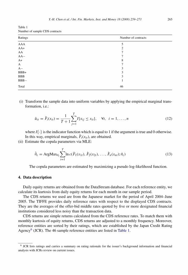
Table 1Number of sample CDS contracts

Ratings Number of contracts

AAA 5AA+ 2AA 7AA− 7A+ 8A 7A− 3BBB+ 3BBB 3BBB− 1

Total 46

(i) Transform the sample data into uniform variables by applying the empirical marginal trans-formation, i.e.:

uit = Fi(xit) = 1

T + 1

T∑j=1

I{xij ≤ xit}, ∀t, i = 1, . . . , n (12)

where I{·} is the indicator function which is equal to 1 if the argument is true and 0 otherwise.In this way, empirical marginals, Fi(xit), are obtained.

(ii) Estimate the copula parameters via MLE:

θc = ArgMaxθc

T∑t=1

ln c(F1(x1t), F2(x2t), . . . , Fn(xnt); θc) (13)

The copula parameters are estimated by maximizing a pseudo log-likelihood function.

4. Data description

Daily equity returns are obtained from the DataStream database. For each reference entity, wecalculate its kurtosis from daily equity returns for each month in our sample period.

The CDS returns we used are from the Japanese market for the period of April 2004–June2005. The TIFFE provides daily reference rates with respect to the displayed CDS contracts.They are the averages of the offer-bid middle rates quoted by five or more designated financialinstitutions considered less noisy than the transaction data.

CDS returns are simple returns calculated from the CDS reference rates. To match them withmonthly kurtosis of equity returns, CDS returns are adjusted to a monthly frequency. Moreover,reference entities are sorted by their ratings, which are established by the Japan Credit RatingAgency6 (JCR). The 46 sample reference entities are listed in Table 1.

6 JCR lists ratings and carries a summary on rating rationale for the issuer’s background information and financialanalysis with JCRs review on current issues.


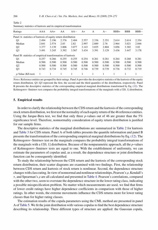
Table 2Summary statistics of kurtosis and its empirical transformation

Ratings AAA AA+ AA AA− A+ A A− BBB+ BBB BBB−Panel A: statistics of kurtosis of equity return distribution

Q1 2.494 2.196 2.376 2.484 2.557 2.336 2.351 2.614 2.614 2.354Median 2.841 2.574 2.83 2.82 2.997 2.889 2.76 2.964 3.021 2.846Q2 3.377 3.139 3.006 3.077 3.143 3.035 2.804 3.056 3.302 3.02Q3 3.491 3.245 3.392 3.567 3.434 3.391 3.129 3.436 3.447 3.178

Panel B: statistics of empirical transformation of kurtosisQ1 0.257 0.266 0.255 0.255 0.254 0.261 0.261 0.264 0.268 0.281Median 0.500 0.500 0.500 0.500 0.500 0.500 0.500 0.500 0.500 0.500Q2 0.500 0.500 0.500 0.500 0.500 0.500 0.500 0.500 0.500 0.500Q3 0.743 0.734 0.745 0.745 0.746 0.739 0.739 0.736 0.732 0.719

p-Value (KS test) 1 1 1 1 1 1 1 1 1 1

Notes: Reference entities are grouped by their ratings. Panel A provides the descriptive statistics of the kurtosis of the equityreturn distribution. Q1–Q3 represent the first, the second and the third quantiles of the distribution, respectively. PanelB presents the descriptive statistics of the corresponding empirical marginal distributions transformed by Eq. (12). TheKolmogorov–Smirnov test compares the probability integral transformations of the marginals with a U[0, 1] distribution.

5. Empirical results

In order to clarify the relationship between the CDS return and the kurtosis of the correspondingstock return distribution, we first test the normality of each equity return of the 46 reference entities.Using the Jarque-Bera test, we find that only three p-values out of 46 are greater than the 5%significance level. Therefore, nonnormality consideration of equity return distribution is justifiedfor our sample firms.

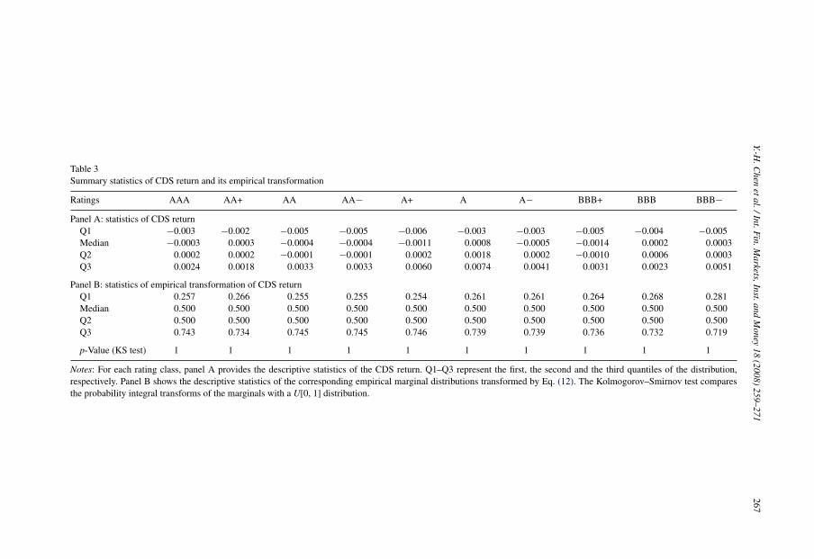
The descriptive statistics of the marginal distributions are summarized in Table 2 for kurtosisand Table 3 for CDS return. Panel A of both tables presents the quantile information and panel Bpresents the transformation of the corresponding empirical marginal distributions by Eq. (12). TheKolmogorov–Smirnov test on the marginals compares the probability integral transformations ofthe marginals with a U[0, 1] distribution. Because of the nonparametric approach, all the p-valuesof Kolmogorov–Smirnov tests are equal to one. With the establishment of uniformity, we canestimate the parameters of copulas and, as a result, the dependence structure or joint distributionfunction can be consequently identified.

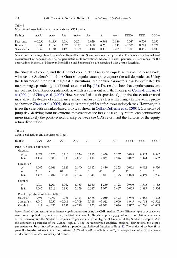
To study the relationship between the CDS return and the kurtosis of the corresponding stockreturn distribution, their scatter diagrams are examined with two findings. First, the relationshipbetween CDS return and kurtosis of stock return is nonlinear. Second, the dependence structurechanges with class rating. In view of nonnormal and nonlinear relationships, Pearson’s ρ, Kendall’sτ, and Spearman’s ρ are all calculated and presented in Table 4. Pearson’s correlations, comparedwith the other two, seem to overstate the dependence structure in the lower rating class, indicatinga possible misspecification problem. No matter which measurements are used, we find that firmsof lower credit ratings have higher dependence coefficients in comparison with those of higherratings. In other words, the extreme movements influence the CDS returns more for lower ratingclasses than for higher rating classes.

The estimation results of the copula parameters using the CML method are presented in panelA of Table 5. We fit the joint distribution with various copulas to find the best dependence structuredescribing its relationship. Three different types of structure are applied: the Gaussian copula,

Y.-H.C

henetal./Int.F

in.Markets,Inst.and

Money

18(2008)

259–271267

Table 3Summary statistics of CDS return and its empirical transformation

Ratings AAA AA+ AA AA− A+ A A− BBB+ BBB BBB−Panel A: statistics of CDS return

Q1 −0.003 −0.002 −0.005 −0.005 −0.006 −0.003 −0.003 −0.005 −0.004 −0.005Median −0.0003 0.0003 −0.0004 −0.0004 −0.0011 0.0008 −0.0005 −0.0014 0.0002 0.0003Q2 0.0002 0.0002 −0.0001 −0.0001 0.0002 0.0018 0.0002 −0.0010 0.0006 0.0003Q3 0.0024 0.0018 0.0033 0.0033 0.0060 0.0074 0.0041 0.0031 0.0023 0.0051

Panel B: statistics of empirical transformation of CDS returnQ1 0.257 0.266 0.255 0.255 0.254 0.261 0.261 0.264 0.268 0.281Median 0.500 0.500 0.500 0.500 0.500 0.500 0.500 0.500 0.500 0.500Q2 0.500 0.500 0.500 0.500 0.500 0.500 0.500 0.500 0.500 0.500Q3 0.743 0.734 0.745 0.745 0.746 0.739 0.739 0.736 0.732 0.719

p-Value (KS test) 1 1 1 1 1 1 1 1 1 1

Notes: For each rating class, panel A provides the descriptive statistics of the CDS return. Q1–Q3 represent the first, the second and the third quantiles of the distribution,respectively. Panel B shows the descriptive statistics of the corresponding empirical marginal distributions transformed by Eq. (12). The Kolmogorov–Smirnov test comparesthe probability integral transforms of the marginals with a U[0, 1] distribution.


Table 4Measures of association between kurtosis and CDS return

Ratings AAA AA+ AA AA− A+ A A− BBB+ BBB BBB−Pearson ρ −0.036 0.293 0.036 0.251 0.029 0.308 0.180 0.087 0.509 0.650Kendall τ 0.040 0.106 0.076 0.122 −0.008 0.290 0.143 −0.002 0.328 0.371Spearman ρ 0.062 0.148 0.123 0.182 −0.018 0.435 0.219 0.001 0.456 0.400

Notes: For each rating class, Pearson’s ρ, Kendall’s τ and Spearman’s ρ are all presented. Pearson’s ρ is a linear-basedmeasurement of dependence. The nonparametric rank correlations, Kendall’s τ and Spearman’s ρ, are robust for theobservations in the tails. Moreover, Kendall’s τ and Spearman’s ρ are associated with copula functions.

the Student’s t copula, and the Gumbel copula. The Gaussian copula serves as the benchmark,whereas the Student’s t and the Gumbel copulas attempt to capture the tail dependence. Usingthe transformed empirical marginal distributions, the copula parameters can be estimated bymaximizing a pseudo log-likelihood function of Eq. (13). The results show that copula parametersare positive for all three copula models, which is consistent with the findings of Collin-Dufresne etal. (2001) and Zhang et al. (2005). However, we find that the proxies of jump risk these authors usedmay affect the degree of significance across various rating classes. In using a firm-specific proxyas shown in Zhang et al. (2005), the sign is more significant for lower rating classes. However, thisis not the case with a market-based proxy, as shown in Collin-Dufresne et al. (2001). Our proxy ofjump risk, deriving from the extreme movement of the individual equity return, can demonstratemore intuitively the positive relationship between the CDS return and the kurtosis of the equityreturn distribution.

Table 5Copula estimations and goodness-of-fit test

Ratings AAA AA+ AA AA− A+ A A− BBB+ BBB BBB−Panel A: Copula estimations

GaussianρGau 0.071 0.223 0.113 0.224 0.015 0.450 0.267 0.048 0.563 0.542ln L 0.154 0.500 0.501 2.062 0.011 2.025 1.246 0.027 3.844 1.602

Student’s tρt 0.062 0.166 0.120 0.190 −0.012 0.440 0.223 −0.002 0.492 0.559ν 7 8 93 7 14 45 45 35 2 2ln L 0.476 0.482 2.009 2.384 0.141 3.811 1.175 1.028 4.859 3.276

Gumbelθ 1.025 1.205 1.042 1.183 1.046 1.280 1.128 0.950 1.573 1.783ln L 0.045 1.018 0.135 3.139 0.587 2.037 0.487 0.065 3.893 2.504

Panel B: goodness-of-fit test (AIC)Gaussian 1.691 0.999 0.998 −2.123 1.978 −2.050 −0.493 1.946 −5.688 −1.205Student’s t 3.047 3.035 −0.018 −0.769 3.718 −3.622 1.650 1.945 −5.718 −2.552Gumbel 1.911 −0.036 1.730 −4.278 0.825 −2.073 1.026 1.867 −5.786 −3.009

Notes: Panel A summarizes the estimated copula parameters using the CML method. Three different types of dependencestructure are applied, i.e., the Gaussian, the Student’s t and the Gumbel copulas. ρGau and ρt are correlation parametersof the Gaussian and the Student’s t copulas, respectively. ν is the degree of freedom of the Student’s t copula. θ isthe dependence parameter of the Gumbel copula. Using the transformed empirical marginal distributions, the copulaparameters can be estimated by maximizing a pseudo log-likelihood function of Eq. (13). The choice of the best fit inpanel B is based on Akaike information criterion (AIC) value, AIC = −2L(θ; x) + 2q, where q is the number of parametersneeded to be estimated in each specific model.


Table 5 shows that copula parameters are consistently higher in the lower ratings for all threecopulas, indicating a strong dependence structure in these classes. For instance, the estimatedparameters of BBB− class are 0.542, 0.559, and 1.783 for the Gaussian, the Student’s t, and theGumbel copulas, respectively. However, the estimated parameters are 0.071, 0.062, and 1.025 forAAA class. Hence, the extreme movements due to jump risk affect the CDS returns more forlower rating classes than for higher ratings. This result is economically intuitive and consistentwith Abid and Naifar (2005), Zhang et al. (2005), and Collin-Dufresne et al. (2001). Our findings,however, stand stronger than those from Norden and Weber (2004), because in their study thelowest rating class does not have the most significant dependence structure. Using the copulamethod, we consistently find that the lowest rating class exhibits the highest significance. Ourempirical evidence concludes that CDS returns of lower rating classes are more sensitive thanthose of higher rating classes to the presence of jumps.

The choice of the best fit is based on the Akaike information criterion (AIC) value. From themaximized log-likelihood in panel A of Table 5, we compute the AIC for each copula and thenrank the copula models accordingly:

AIC = −2L(θ; x) + 2q, (14)

where q is the number of parameters needed to be estimated in each specific model. Both theGaussian and the Gumbel copulas need to estimate one parameter, i.e., ρGau and θ, respectively,while the Student’s t copula has two correlation parameters ρt and a degree of freedom ν. As theestimating procedure for the Student’s t copula is computationally cumbersome,7 the alternativeMashal and Zeevi (2002) method is applied. By taking advantage of the properties of the Student’st copula, ρt is estimated via a rank correlation estimator, namely the Kendall’s τ, as follows:

ρτ = 2

πarcsin ρt. (15)

Given this,8 we can find the degree of freedom that maximizes the log-likelihood function fora given ρt.

Panel B of Table 5 depicts the AIC values for the three chosen copulas. For BBB− and BBBclasses, the lowest AIC values are −3.009 and −5.786, respectively, and both come from theGumbel copula. Meanwhile, the AIC values for the Student’s t copula are smaller than thoseof the Gaussian copula. Thus, for lower rating classes, we find that the Gumbel copula showsthe lowest value of AIC, while the Student’s t copula performs slightly better than the Gaussiancopula. The result suggests that tail dependence is evident in our samples, and the Gumbel is thebest fitting copula compared with the Gaussian and the Student’s t copulas.

To further examine the tail dependence, Table 6 reports the estimated coefficients of tail depen-dence for the Student’s t and the Gumbel copulas based on Eqs. (10) and (11), respectively. Asthe standard Student’s t distribution is symmetric, the estimated coefficient represents not onlythe upper but also the lower tail dependence. In contrast, the coefficient from the Gumbel copulacaptures only the upper tail dependence. As shown in Table 6, for BBB− class, the coefficientsof tail dependence for the Student’s t and the Gumbel copulas are 0.42 and 0.525, respectively,and estimated coefficients are 0.387 and 0.446 for both copulas in BBB class. Nevertheless, esti-mated coefficients are only 0.029 and 0.033 for both copulas in AAA class. Therefore, the taildependence exists in lower rating classes for both copulas.

7 Due to its simultaneous estimation for parameter ρt and ν.8 A proof of this result can be found in Fang and Fang (2002).


Table 6Estimated coefficients of tail dependence

Ratings AAA AA+ AA AA− A+ A A− BBB+ BBB BBB−Student’s t, λt 0.029 0.032 0 0.048 0.001 0 0 0 0.387 0.420Gumbel, λGum 0.033 0.223 0.055 0.204 0.059 0.282 0.151 −0.075 0.446 0.525

Notes: This table reports the estimated coefficients of tail dependence for the Student’s t and the Gumbel copulas basedon Eqs. (10) and (11), respectively.

Fig. 1. Copula density plot of kurtosis of equity return and CDS return. Notes: To visualize the joint probability distributionsand the dependence structures between variables, figure shows the surfaces of the copula densities for the lowest ratingclass.

Given the estimated copula parameters, the surface of the copula densities for the lowest ratingclasses can be expressed. We present these densities in Fig. 1 to visualize their joint probabilitydistributions and the dependence structures between variables. As can be seen, the densities of theGaussian and the Student’s t copulas are symmetric, with thicker tails for the Student’s t copula.Meanwhile, the Gumbel copula exhibits the upper tail dependence as expected.

6. Conclusion

Understanding the CDS is particularly important because of its popularity and liquidity in thecredit markets. However, its empirical investigation has been limited by data availability. Thispaper specifically focuses on the empirical analysis of the dependence structure between theCDS return and the kurtosis of the corresponding equity return distribution. Kurtosis persistentlyexhibits in the financial markets and has a strong impact on risk management. It measures theextreme movement in equity returns and indicates the tendency of jump events. In addition todemonstrating the dependence structure, we further discuss the implications of our findings. To


take both nonlinear and non-Gaussian relationships into account, we employ a copula-basedmethodology. Three copula functions, namely the Gaussian, the Student’s t, and the Gumbelcopulas, are explored in model fitting.

Daily CDS rates of 46 reference entities are collected from the TIFFE, covering the period fromApril 2004 to June 2005. First, we find that CDS returns in lower rating class are more sensitive tojump risk than those in the higher ratings. Second, the dependence structure is positive, indicatingthat protection sellers ask for higher CDS return to compensate for a higher tendency of jumps.Third, the Gumbel copula is the best fitting model for lower rating classes based on its lowest AICvalue, and the Student’s t performs better than the Gaussian copula, at least to the lower ratingclasses. Fourth, the dependence structure is asymmetric, orienting toward the upper side. Becausehigher probability of comovement occurs in the right tails, the upper tail dependence becomesmore significant as jump events and CDS returns increase simultaneously.

Since observed tail dependence is asymmetric in this study, it is necessary to take kurtosis intoaccount when pricing CDS. Otherwise, the true price of the credit risk might be underestimated.Similarly, the portfolio choice and hedging strategy may be more complicated when dependencestructure between assets are considered. These are left for future study.

References

Abid, F., Naifar, N., 2005. The impact of stock returns volatility on credit default swap rates: a copula study. InternationalJournal of Theoretical and Applied Finance 8, 1135–1155.

Andersen, T.G., Benzoni, L., Lund, J., 2002. An empirical investigation of continuous-time equity return models. Journalof Finance 57, 1239–1284.

Andreev, A., Kanto, A., 2005. Conditional value-at-risk estimation using non-integer values of degrees of freedom inStudent’s t-distribution. The Journal of Risk 7, 55–61.

Bates, D.S., 1996. Jumps and stochastic volatility: exchange rate processes implicit in deutsche mark options. Review ofFinancial Studies 9, 69–107.

Bee, M., 2004. Modelling credit default swap spreads by means of normal mixtures and copulas. Applied MathematicalFinance 11, 125–146.

Benkert, C., 2004. Explaining credit default swap premia. Journal of Futures Markets 24, 71–92.Blanco, R., Brennan, S., Marsh, I.W., 2005. An empirical analysis of the dynamic relation between investment-grade

bonds and credit default swaps. Journal of Finance 60, 2255–2281.Cariboni, J., Schoutens, W., 2004. Pricing Credit Default Swaps under Levy Models. Working Paper. European Commis-

sion and K.U. Leuven.Collin-Dufresne, P., Goldstein, R.S., Martin, J.S., 2001. The determinants of credit spread changes. Journal of Finance

56, 2177–2207.Drost, F.C., Nijman, T.E., Werker, B.J.M., 1998. Estimation and testing in models containing both jumps and conditional

heteroscedasticity. Journal of Business and Economic Statistics 16, 237–243.Fang, H., Fang, K., 2002. The meta-elliptical distributions with given marginals. Journal of Multivariate Analysis 82,

1–16.Longin, F., Solnik, B., 2001. Extreme correlation of international equity markets. Journal of Finance 56, 649–676.Mashal, R., Zeevi, A., 2002. Beyond Correlation: Extreme Co-movements between Financial Assets. Working Paper.

Columbia University.Nelsen, R.B., 1999. An Introduction to Copulas. Springer-Verlag, New York.Norden, L., Weber, M., 2004. The Comovement of Credit Default Swap, Bond and Stock Markets: An Empirical Analysis.

Working Paper. University of Mannheim.Zhang, B.Y., Zhou, H., Zhu, H., 2005. Explaining Credit Default Swap Spreads with the Equity Volatility and Jump Risks

of Individual Firms. Working Paper. Bank for International Settlements.Zhou, C., 2001. The term structure of credit spreads with jump risk. Journal of Banking and Finance 25, 2015–2040.Zhu, H., 2006. An empirical comparison of credit spreads between the bond market and the credit default swap market.

Journal of Financial Services Research 29, 211–235.

dependence structure between the credit default swap return and the kurtosis of the equity return...

Documents