DEPENDENT TYPES IN HASKELL:THEORY AND PRACTICE

Richard A. Eisenberg

A DISSERTATION

in

Computer and Information Sciences

Presented to the Faculties of the University of Pennsylvaniain

Partial Fulfillment of the Requirements for theDegree of Doctor of Philosophy

2016

Supervisor of Dissertation

Stephanie Weirich, PhDProfessor of CIS

Graduate Group Chairperson

Lyle Ungar, PhDProfessor of CIS

Dissertation CommitteeRajeev Alur, PhD (Professor of CIS)Simon Peyton Jones (Principal Researcher, Microsoft Research)Benjamin Pierce, PhD (Professor of CIS; Committee Chair)Steve Zdancewic, PhD (Professor of CIS)

DEPENDENT TYPES IN HASKELL: THEORY AND PRACTICE

COPYRIGHT

2016

Richard A. Eisenberg

This work is licensed under a Creative Commons Attribution 4.0International License. To view a copy of this license, visit

http://creativecommons.org/licenses/by/4.0/

The complete source code for this document is available from

http://github.com/goldfirere/thesis

To Amanda,

who has given more of herself toward this doctorate than I could ever ask.

iii

Acknowledgments

I have so many people to thank.First and foremost, I thank my sponsors. This material is based upon work

supported by the National Science Foundation under Grant No. 1116620. I alsogratefully acknowledge my Microsoft Research Graduate Student Fellowship, whichhas supported me in my final two years.

Thanks to the Haskell community, who have welcomed this relative newcomerwith open arms and minds. My first line of Haskell was written only in 2011! Thereare far too many to name, but I’ll call out Ben Gamari and Austin Seipp for theircommendable job at shepherding the GHC development process.

I am not one for large displays of school spirit. Nevertheless, I cannot imagine abetter place to get my doctorate than Penn. I will remain passionate in my advocacyfor this graduate program for many years to come.

The PLClub at Penn has been a constant source of camaraderie, help on varioussubjects, and great talks. Thanks to Jianzhou, Mike, Chris, Marco, Emilio, Catalin,Benoît, Benoît, Maxime, Delphine, Vilhelm, Daniel, Bob, Justin, Arthur, Antal,Jennifer, Dmitri, William, Leo, Robert, Antoine, and Pedro.

Thanks to “FC crew” who put up with my last-minute reminders and frequentrescheduling. David Darais, Iavor Diatchki, Kenny Foner, Andres Löh, Pedro Magal-hães, Conor McBride: thanks for all the great discussions, and I look forward to manymore to come.

I can thank Joachim Breitner for helping me with perhaps the hardest part ofthis dissertation: not working on roles, a topic I have tried to escape for the betterpart of three years. Joachim spearheaded our papers on the subject, and his excellentorganization at writing papers will serve as a template for my future projects.

Jan Stolarek co-authored several papers with me and his probing questions helpedme greatly to understand certain aspects of Dependent Haskell better. In particular,the idea of having matchable vs. unmatchable functions is directly due to work donein concert with Jan.

Adam Gundry bulldozed the path for me. His dissertation was something of a roadmap for mine, and I always learn from his insight.

Sincere thanks to Peter-Michael Osera for leading the way toward a position at aliberal arts college and for much humor, some of it appropriate.

I owe a debt of gratitude to Brent Yorgey. He decided not to continue pursuing

iv

dependent types in Haskell just as I came along. He also (co-)wrote a grant that wasapproved just in time to free up his advisor to take on another student. Much of mysuccess is due to Brent’s paving the way for me.

Dimitrios Vytiniotis was a welcoming co-host at Microsoft Research when I wasthere. I still have scars from the many hours of battling the proof dragon in his office.

None of this, quite literally, would be possible without the leap of faith taken byBenjamin Pierce, to whom I argued for my acceptance to Penn, over the phone, on ashared line in the middle of a campground in the Caribbean, surrounded by childrenand families enjoying their vacation. A condition of my acceptance was that I wouldnot work with Stephanie, who had no room for me, despite our matching interests. Itrust Benjamin does not regret this decision, even though I violated this condition.

I offer a heartfelt thanks to Steve Zdancewic. From the beginning of my timeat Penn, I felt entirely at home knocking on his door at any time to ask for adviceor mentorship. I did not often take advantage of this, but it was indeed a comfortknowing I could seek him out.

I cannot express enough gratitude toward my family, new and old, who havesupported me in every way possible.

Simon Peyton Jones is a visionary leader for the Haskell community, holding all ofus together on the steady stride toward a more perfect language. Simon’s mentorshipto me, personally, has been invaluable. It is such an honor to work alongside you,Simon, and I look forward to much collaboration to come.

Stephanie Weirich is the best advisor a student could ask for. She is insightful, fullof energy and ideas, and simply has an intuitive grasp on how best to nudge me along.And she’s brilliant. Stephanie, thanks for pulling me out of your Haskell programmingclass five years ago—that’s what started us on this adventure. Somehow, you mademe feel right away that I was having interesting and novel ideas; in retrospect, manyof them were really yours, all along. This is surely the sign of excellent academicadvising.

I am left to thank my wife Amanda and daughter Emma. Both have been with meevery step of the way. Well, Emma missed some steps as she wasn’t walking for thefirst year or so, having been born two months before I started at Penn. But tonight,she accurately summarized to Amanda the difference between Dependent Haskell andIdris (one is a change to an existing language while the other is a brand new one, butboth have dependent types). Children grow fast, and I know Emma is eager for theday when I can finally explain to her what it is I do all day.

And for Amanda, these words will have to do, because no words can truly expresshow I feel: I love you, and thank you.

Richard A. EisenbergAugust 2016

v

ABSTRACTDEPENDENT TYPES IN HASKELL: THEORY AND PRACTICE

Richard A. Eisenberg

Stephanie Weirich

Haskell, as implemented in the Glasgow Haskell Compiler (GHC), has been adding

new type-level programming features for some time. Many of these features—general-

ized algebraic datatypes (GADTs), type families, kind polymorphism, and promoted

datatypes—have brought Haskell to the doorstep of dependent types. Many depen-

dently typed programs can even currently be encoded, but often the constructions are

painful.

In this dissertation, I describe Dependent Haskell, which supports full dependent

types via a backward-compatible extension to today’s Haskell. An important contribu-

tion of this work is an implementation, in GHC, of a portion of Dependent Haskell,

with the rest to follow. The features I have implemented are already released, in

GHC 8.0. This dissertation contains several practical examples of Dependent Haskell

code, a full description of the differences between Dependent Haskell and today’s

Haskell, a novel dependently typed lambda-calculus (called Pico) suitable for use as

an intermediate language for compiling Dependent Haskell, and a type inference and

elaboration algorithm, Bake, that translates Dependent Haskell to type-correct Pico.

Full proofs of type safety of Pico and the soundness of Bake are included in the

appendix.

vi

Contents

1 Introduction 11.1 Contributions . . . . . . . . . . . . . . . . . . . . . . . . . . . . . . . 11.2 Implications beyond Haskell . . . . . . . . . . . . . . . . . . . . . . . 4

2 Preliminaries 62.1 Type classes and dictionaries . . . . . . . . . . . . . . . . . . . . . . . 62.2 Families . . . . . . . . . . . . . . . . . . . . . . . . . . . . . . . . . . 7

2.2.1 Type families . . . . . . . . . . . . . . . . . . . . . . . . . . . 72.2.2 Data families . . . . . . . . . . . . . . . . . . . . . . . . . . . 9

2.3 Rich kinds . . . . . . . . . . . . . . . . . . . . . . . . . . . . . . . . . 92.3.1 Kinds in Haskell98 . . . . . . . . . . . . . . . . . . . . . . . . 92.3.2 Promoted datatypes . . . . . . . . . . . . . . . . . . . . . . . 102.3.3 Kind polymorphism . . . . . . . . . . . . . . . . . . . . . . . . 102.3.4 Constraint kinds . . . . . . . . . . . . . . . . . . . . . . . . . 11

2.4 Generalized algebraic datatypes . . . . . . . . . . . . . . . . . . . . . 122.5 Higher-rank types . . . . . . . . . . . . . . . . . . . . . . . . . . . . . 132.6 Scoped type variables . . . . . . . . . . . . . . . . . . . . . . . . . . . 142.7 Functional dependencies . . . . . . . . . . . . . . . . . . . . . . . . . 15

3 Motivation 163.1 Eliminating erroneous programs . . . . . . . . . . . . . . . . . . . . . 16

3.1.1 Simple example: Length-indexed vectors . . . . . . . . . . . . 163.1.2 A strongly typed simply typed λ-calculus interpreter . . . . . 213.1.3 Type-safe database access with an inferred schema . . . . . . 263.1.4 Machine-checked sorting algorithms . . . . . . . . . . . . . . . 32

3.2 Encoding hard-to-type programs . . . . . . . . . . . . . . . . . . . . . 333.2.1 Variable-arity zipWith . . . . . . . . . . . . . . . . . . . . . . 333.2.2 Typed reflection . . . . . . . . . . . . . . . . . . . . . . . . . . 363.2.3 Algebraic effects . . . . . . . . . . . . . . . . . . . . . . . . . . 39

3.3 Why Haskell? . . . . . . . . . . . . . . . . . . . . . . . . . . . . . . . 473.3.1 Increased reach . . . . . . . . . . . . . . . . . . . . . . . . . . 473.3.2 Backward-compatible type inference . . . . . . . . . . . . . . . 473.3.3 No termination or totality checking . . . . . . . . . . . . . . . 48

vii

3.3.4 GHC is an industrial-strength compiler . . . . . . . . . . . . . 493.3.5 Manifest type erasure properties . . . . . . . . . . . . . . . . . 493.3.6 Type-checker plugin support . . . . . . . . . . . . . . . . . . . 503.3.7 Haskellers want dependent types . . . . . . . . . . . . . . . . 50

4 Dependent Haskell 514.1 Dependent Haskell is dependently typed . . . . . . . . . . . . . . . . 514.2 Quantifiers . . . . . . . . . . . . . . . . . . . . . . . . . . . . . . . . . 54

4.2.1 Dependency . . . . . . . . . . . . . . . . . . . . . . . . . . . . 544.2.2 Relevance . . . . . . . . . . . . . . . . . . . . . . . . . . . . . 554.2.3 Visibility . . . . . . . . . . . . . . . . . . . . . . . . . . . . . . 564.2.4 Matchability . . . . . . . . . . . . . . . . . . . . . . . . . . . . 584.2.5 The twelve quantifiers of Dependent Haskell . . . . . . . . . . 59

4.3 Pattern matching . . . . . . . . . . . . . . . . . . . . . . . . . . . . . 604.3.1 A simple pattern match . . . . . . . . . . . . . . . . . . . . . 614.3.2 A GADT pattern match . . . . . . . . . . . . . . . . . . . . . 614.3.3 Dependent pattern match . . . . . . . . . . . . . . . . . . . . 62

4.4 Discussion . . . . . . . . . . . . . . . . . . . . . . . . . . . . . . . . . 634.4.1 Type : Type . . . . . . . . . . . . . . . . . . . . . . . . . . . 634.4.2 Inferring Π . . . . . . . . . . . . . . . . . . . . . . . . . . . . 634.4.3 Roles and dependent types . . . . . . . . . . . . . . . . . . . . 644.4.4 Impredicativity, or lack thereof . . . . . . . . . . . . . . . . . 644.4.5 Running proofs . . . . . . . . . . . . . . . . . . . . . . . . . . 654.4.6 Import and export lists . . . . . . . . . . . . . . . . . . . . . . 664.4.7 Type-checking is undecidable . . . . . . . . . . . . . . . . . . 66

4.5 Conclusion . . . . . . . . . . . . . . . . . . . . . . . . . . . . . . . . . 66

5 Pico: The intermediate language 685.1 Overview . . . . . . . . . . . . . . . . . . . . . . . . . . . . . . . . . . 68

5.1.1 Features of Pico . . . . . . . . . . . . . . . . . . . . . . . . . 695.1.2 Design requirements for Pico . . . . . . . . . . . . . . . . . . 725.1.3 Other applications of Pico . . . . . . . . . . . . . . . . . . . 745.1.4 No roles in Pico . . . . . . . . . . . . . . . . . . . . . . . . . 74

5.2 A formal specification of Pico . . . . . . . . . . . . . . . . . . . . . . 755.3 Contexts Γ and relevance annotations . . . . . . . . . . . . . . . . . . 795.4 Signatures Σ and type constants H . . . . . . . . . . . . . . . . . . . 81

5.4.1 Signature validity . . . . . . . . . . . . . . . . . . . . . . . . . 815.4.2 Looking up type constants . . . . . . . . . . . . . . . . . . . . 82

5.5 Examples . . . . . . . . . . . . . . . . . . . . . . . . . . . . . . . . . 865.5.1 isEmpty . . . . . . . . . . . . . . . . . . . . . . . . . . . . . . 875.5.2 replicate . . . . . . . . . . . . . . . . . . . . . . . . . . . . . . 885.5.3 append . . . . . . . . . . . . . . . . . . . . . . . . . . . . . . . 895.5.4 safeHead . . . . . . . . . . . . . . . . . . . . . . . . . . . . . . 91

viii

5.6 Types τ . . . . . . . . . . . . . . . . . . . . . . . . . . . . . . . . . . 915.6.1 Abstractions . . . . . . . . . . . . . . . . . . . . . . . . . . . . 925.6.2 Applications . . . . . . . . . . . . . . . . . . . . . . . . . . . . 925.6.3 Kind casts . . . . . . . . . . . . . . . . . . . . . . . . . . . . . 935.6.4 fix . . . . . . . . . . . . . . . . . . . . . . . . . . . . . . . . . 935.6.5 case . . . . . . . . . . . . . . . . . . . . . . . . . . . . . . . . 93

5.7 Operational semantics . . . . . . . . . . . . . . . . . . . . . . . . . . 995.7.1 Values . . . . . . . . . . . . . . . . . . . . . . . . . . . . . . . 995.7.2 Reduction . . . . . . . . . . . . . . . . . . . . . . . . . . . . . 1005.7.3 Congruence forms . . . . . . . . . . . . . . . . . . . . . . . . . 1015.7.4 Push rules . . . . . . . . . . . . . . . . . . . . . . . . . . . . . 101

5.8 Coercions γ . . . . . . . . . . . . . . . . . . . . . . . . . . . . . . . . 1035.8.1 Equality is heterogeneous . . . . . . . . . . . . . . . . . . . . 1035.8.2 Equality is hypothetical . . . . . . . . . . . . . . . . . . . . . 1055.8.3 Equality is coherent . . . . . . . . . . . . . . . . . . . . . . . . 1055.8.4 Equality is an equivalence . . . . . . . . . . . . . . . . . . . . 1065.8.5 Equality is (almost) congruent . . . . . . . . . . . . . . . . . . 1065.8.6 Equality can be decomposed . . . . . . . . . . . . . . . . . . . 1125.8.7 Equality includes β-reduction . . . . . . . . . . . . . . . . . . 1175.8.8 Discussion . . . . . . . . . . . . . . . . . . . . . . . . . . . . . 117

5.9 The S_KPush rule . . . . . . . . . . . . . . . . . . . . . . . . . . . . 1185.10 Metatheory: Consistency . . . . . . . . . . . . . . . . . . . . . . . . . 122

5.10.1 Compatibility . . . . . . . . . . . . . . . . . . . . . . . . . . . 1235.10.2 The parallel rewrite relation . . . . . . . . . . . . . . . . . . . 1245.10.3 Completeness of the rewrite relation . . . . . . . . . . . . . . 1275.10.4 From completeness to consistency . . . . . . . . . . . . . . . . 1275.10.5 Related consistency proofs . . . . . . . . . . . . . . . . . . . . 128

5.11 Metatheory: Type erasure . . . . . . . . . . . . . . . . . . . . . . . . 1305.11.1 The untyped λ-calculus . . . . . . . . . . . . . . . . . . . . . . 1305.11.2 Simulation . . . . . . . . . . . . . . . . . . . . . . . . . . . . . 1325.11.3 Types do not prevent evaluation . . . . . . . . . . . . . . . . . 132

5.12 Design decisions . . . . . . . . . . . . . . . . . . . . . . . . . . . . . . 1335.12.1 Coercions are not types . . . . . . . . . . . . . . . . . . . . . . 1335.12.2 Putting braces around irrelevant arguments . . . . . . . . . . 1335.12.3 Including types’ kinds in propositions . . . . . . . . . . . . . . 134

5.13 Extensions . . . . . . . . . . . . . . . . . . . . . . . . . . . . . . . . . 1345.13.1 let . . . . . . . . . . . . . . . . . . . . . . . . . . . . . . . . . 1345.13.2 A primitive equality check . . . . . . . . . . . . . . . . . . . . 1355.13.3 Splitting type applications . . . . . . . . . . . . . . . . . . . . 1375.13.4 Levity polymorphism . . . . . . . . . . . . . . . . . . . . . . . 1385.13.5 The (→) type constructor . . . . . . . . . . . . . . . . . . . . 139

5.14 Conclusion . . . . . . . . . . . . . . . . . . . . . . . . . . . . . . . . . 140

ix

6 Type inference and elaboration 1416.1 Overview . . . . . . . . . . . . . . . . . . . . . . . . . . . . . . . . . . 1426.2 Haskell grammar . . . . . . . . . . . . . . . . . . . . . . . . . . . . . 144

6.2.1 Dependent Haskell modalities . . . . . . . . . . . . . . . . . . 1456.2.2 let should not be generalized . . . . . . . . . . . . . . . . . . . 1466.2.3 Omissions from the Haskell grammar . . . . . . . . . . . . . . 146

6.3 Unification variables . . . . . . . . . . . . . . . . . . . . . . . . . . . 1476.3.1 Zonking . . . . . . . . . . . . . . . . . . . . . . . . . . . . . . 1486.3.2 Additions to Pico judgments . . . . . . . . . . . . . . . . . . 1496.3.3 Untouchable unification variables . . . . . . . . . . . . . . . . 150

6.4 Bidirectional type-checking . . . . . . . . . . . . . . . . . . . . . . . . 1526.4.1 Invisibility . . . . . . . . . . . . . . . . . . . . . . . . . . . . . 1536.4.2 Subsumption . . . . . . . . . . . . . . . . . . . . . . . . . . . 1546.4.3 Skolemization . . . . . . . . . . . . . . . . . . . . . . . . . . . 156

6.5 Generalization . . . . . . . . . . . . . . . . . . . . . . . . . . . . . . . 1586.6 Type inference algorithm . . . . . . . . . . . . . . . . . . . . . . . . . 160

6.6.1 Function application . . . . . . . . . . . . . . . . . . . . . . . 1606.6.2 Mediating between checking and synthesis . . . . . . . . . . . 1626.6.3 case expressions . . . . . . . . . . . . . . . . . . . . . . . . . 1636.6.4 Checking λ-expressions . . . . . . . . . . . . . . . . . . . . . . 163

6.7 Program elaboration . . . . . . . . . . . . . . . . . . . . . . . . . . . 1646.7.1 Declarations . . . . . . . . . . . . . . . . . . . . . . . . . . . . 1656.7.2 Programs . . . . . . . . . . . . . . . . . . . . . . . . . . . . . 166

6.8 Metatheory . . . . . . . . . . . . . . . . . . . . . . . . . . . . . . . . 1666.8.1 Soundness . . . . . . . . . . . . . . . . . . . . . . . . . . . . . 1676.8.2 Conservativity with respect to OutsideIn . . . . . . . . . . . 1716.8.3 Conservativity with respect to System SB . . . . . . . . . . . 173

6.9 Practicalities . . . . . . . . . . . . . . . . . . . . . . . . . . . . . . . 1746.9.1 Class constraints . . . . . . . . . . . . . . . . . . . . . . . . . 1746.9.2 Scoped type variables . . . . . . . . . . . . . . . . . . . . . . . 1756.9.3 Correspondence between Bake and GHC . . . . . . . . . . . 1766.9.4 Unification variables in GHC . . . . . . . . . . . . . . . . . . . 1766.9.5 Constraint vs. Type . . . . . . . . . . . . . . . . . . . . . . . 177

6.10 Discussion . . . . . . . . . . . . . . . . . . . . . . . . . . . . . . . . . 1776.10.1 Further desirable properties of the solver . . . . . . . . . . . . 1776.10.2 No coercion abstractions . . . . . . . . . . . . . . . . . . . . . 1796.10.3 Comparison to Gundry [37] . . . . . . . . . . . . . . . . . . . 180

6.11 Conclusion . . . . . . . . . . . . . . . . . . . . . . . . . . . . . . . . . 181

7 Implementation 1827.1 Current state of implementation . . . . . . . . . . . . . . . . . . . . . 182

7.1.1 Implemented in GHC 8 . . . . . . . . . . . . . . . . . . . . . . 1827.1.2 Implemented in singletons . . . . . . . . . . . . . . . . . . . . 183

x

7.1.3 Implementation to be completed . . . . . . . . . . . . . . . . . 1857.2 Type equality . . . . . . . . . . . . . . . . . . . . . . . . . . . . . . . 186

7.2.1 Properties of a new definitional equality ≡ . . . . . . . . . . . 1877.2.2 Replacing = with ≡ . . . . . . . . . . . . . . . . . . . . . . . 1887.2.3 Implementation of ≡ . . . . . . . . . . . . . . . . . . . . . . . 189

7.3 Unification . . . . . . . . . . . . . . . . . . . . . . . . . . . . . . . . . 1897.4 Parsing ? . . . . . . . . . . . . . . . . . . . . . . . . . . . . . . . . . 1917.5 Promoting base types . . . . . . . . . . . . . . . . . . . . . . . . . . . 192

8 Related and future work 1938.1 Comparison to Gundry’s thesis . . . . . . . . . . . . . . . . . . . . . 193

8.1.1 Unsaturated functions in types . . . . . . . . . . . . . . . . . 1938.1.2 Support for type families . . . . . . . . . . . . . . . . . . . . . 1948.1.3 Axioms . . . . . . . . . . . . . . . . . . . . . . . . . . . . . . 1948.1.4 Type erasure . . . . . . . . . . . . . . . . . . . . . . . . . . . 195

8.2 Comparison to Idris . . . . . . . . . . . . . . . . . . . . . . . . . . . . 1958.2.1 Backward compatibility . . . . . . . . . . . . . . . . . . . . . 1958.2.2 Type erasure . . . . . . . . . . . . . . . . . . . . . . . . . . . 1958.2.3 Type inference . . . . . . . . . . . . . . . . . . . . . . . . . . 1968.2.4 Editor integration . . . . . . . . . . . . . . . . . . . . . . . . . 197

8.3 Comparison to Cayenne . . . . . . . . . . . . . . . . . . . . . . . . . 1978.3.1 Type erasure . . . . . . . . . . . . . . . . . . . . . . . . . . . 1988.3.2 Coercion assumptions . . . . . . . . . . . . . . . . . . . . . . . 1988.3.3 A hierarchy of sorts . . . . . . . . . . . . . . . . . . . . . . . . 1988.3.4 Metatheory . . . . . . . . . . . . . . . . . . . . . . . . . . . . 1998.3.5 Modules . . . . . . . . . . . . . . . . . . . . . . . . . . . . . . 1998.3.6 Conclusion . . . . . . . . . . . . . . . . . . . . . . . . . . . . . 199

8.4 Comparison to Liquid Haskell . . . . . . . . . . . . . . . . . . . . . . 1998.5 Comparison to Trellys . . . . . . . . . . . . . . . . . . . . . . . . . . 2008.6 Invisibility in other languages . . . . . . . . . . . . . . . . . . . . . . 2018.7 Type erasure and relevance in other languages . . . . . . . . . . . . . 2028.8 Future directions . . . . . . . . . . . . . . . . . . . . . . . . . . . . . 2048.9 Conclusion . . . . . . . . . . . . . . . . . . . . . . . . . . . . . . . . . 205

A Typographical conventions 206

B Pico typing rules, in full 207B.1 Type constants . . . . . . . . . . . . . . . . . . . . . . . . . . . . . . 207B.2 Types . . . . . . . . . . . . . . . . . . . . . . . . . . . . . . . . . . . 207B.3 Coercions . . . . . . . . . . . . . . . . . . . . . . . . . . . . . . . . . 209B.4 Vectors . . . . . . . . . . . . . . . . . . . . . . . . . . . . . . . . . . . 213B.5 Contexts . . . . . . . . . . . . . . . . . . . . . . . . . . . . . . . . . . 214B.6 Small-step operational semantics . . . . . . . . . . . . . . . . . . . . 215

xi

B.7 Consistency . . . . . . . . . . . . . . . . . . . . . . . . . . . . . . . . 217B.8 Small-step operational semantics of erased expressions . . . . . . . . . 219

C Proofs about Pico 221C.1 Auxiliary definitions . . . . . . . . . . . . . . . . . . . . . . . . . . . 221C.2 Structural properties . . . . . . . . . . . . . . . . . . . . . . . . . . . 221

C.2.1 Relevant contexts . . . . . . . . . . . . . . . . . . . . . . . . . 221C.2.2 Regularity, Part I . . . . . . . . . . . . . . . . . . . . . . . . . 222C.2.3 Weakening . . . . . . . . . . . . . . . . . . . . . . . . . . . . . 223C.2.4 Scoping . . . . . . . . . . . . . . . . . . . . . . . . . . . . . . 223

C.3 Unification . . . . . . . . . . . . . . . . . . . . . . . . . . . . . . . . . 224C.4 Determinacy . . . . . . . . . . . . . . . . . . . . . . . . . . . . . . . . 224C.5 Vectors . . . . . . . . . . . . . . . . . . . . . . . . . . . . . . . . . . . 225C.6 Substitution . . . . . . . . . . . . . . . . . . . . . . . . . . . . . . . . 227C.7 Type constants . . . . . . . . . . . . . . . . . . . . . . . . . . . . . . 230C.8 Regularity, Part II . . . . . . . . . . . . . . . . . . . . . . . . . . . . 231C.9 Preservation . . . . . . . . . . . . . . . . . . . . . . . . . . . . . . . . 236C.10 Consistency . . . . . . . . . . . . . . . . . . . . . . . . . . . . . . . . 243C.11 Progress . . . . . . . . . . . . . . . . . . . . . . . . . . . . . . . . . . 258C.12 Type erasure . . . . . . . . . . . . . . . . . . . . . . . . . . . . . . . 261C.13 Congruence . . . . . . . . . . . . . . . . . . . . . . . . . . . . . . . . 264

D Type inference rules, in full 268D.1 Closing substitution validity . . . . . . . . . . . . . . . . . . . . . . . 268D.2 Additions to Pico judgments . . . . . . . . . . . . . . . . . . . . . . . 268D.3 Zonker validity . . . . . . . . . . . . . . . . . . . . . . . . . . . . . . 269D.4 Synthesis . . . . . . . . . . . . . . . . . . . . . . . . . . . . . . . . . . 269D.5 Checking . . . . . . . . . . . . . . . . . . . . . . . . . . . . . . . . . . 271D.6 Inference for auxiliary syntactic elements . . . . . . . . . . . . . . . . 274D.7 Kind conversions . . . . . . . . . . . . . . . . . . . . . . . . . . . . . 276D.8 Instantiation . . . . . . . . . . . . . . . . . . . . . . . . . . . . . . . . 277D.9 Subsumption . . . . . . . . . . . . . . . . . . . . . . . . . . . . . . . 278D.10 Generalization . . . . . . . . . . . . . . . . . . . . . . . . . . . . . . . 279D.11 Programs . . . . . . . . . . . . . . . . . . . . . . . . . . . . . . . . . 279

E Proofs about the Bake algorithm 281E.1 Type inference judgment properties . . . . . . . . . . . . . . . . . . . 281E.2 Properties adopted from Appendix C . . . . . . . . . . . . . . . . . . 281E.3 Regularity . . . . . . . . . . . . . . . . . . . . . . . . . . . . . . . . . 284E.4 Zonking . . . . . . . . . . . . . . . . . . . . . . . . . . . . . . . . . . 285E.5 Solver . . . . . . . . . . . . . . . . . . . . . . . . . . . . . . . . . . . 287E.6 Supporting functions . . . . . . . . . . . . . . . . . . . . . . . . . . . 287E.7 Supporting lemmas . . . . . . . . . . . . . . . . . . . . . . . . . . . . 287

xii

E.8 Generalization . . . . . . . . . . . . . . . . . . . . . . . . . . . . . . . 289E.9 Soundness . . . . . . . . . . . . . . . . . . . . . . . . . . . . . . . . . 291E.10 Conservativity with respect to OutsideIn . . . . . . . . . . . . . . . 307E.11 Conservativity with respect to System SB . . . . . . . . . . . . . . . 309

F Proofs about Pico≡ 312F.1 The Pico≡ type system . . . . . . . . . . . . . . . . . . . . . . . . . 312F.2 Properties of ≡ . . . . . . . . . . . . . . . . . . . . . . . . . . . . . . 322F.3 Lemmas adapted from Appendix C . . . . . . . . . . . . . . . . . . . 324F.4 Soundness of Pico≡ . . . . . . . . . . . . . . . . . . . . . . . . . . . 324

Bibliography 327

xiii

List of Figures

3.1 Database tables used in Section 3.1.3. . . . . . . . . . . . . . . . . . . 273.2 The queryDB function . . . . . . . . . . . . . . . . . . . . . . . . . . 273.3 Types used in the example of Section 3.1.3. . . . . . . . . . . . . . . . 28

4.1 The twelve quantifiers of Dependent Haskell . . . . . . . . . . . . . . 59

5.1 The grammar of Pico . . . . . . . . . . . . . . . . . . . . . . . . . . 765.2 Notation conventions of Pico . . . . . . . . . . . . . . . . . . . . . . 775.3 Judgments used in the definition of Pico . . . . . . . . . . . . . . . . 785.4 A brief introduction to coercions . . . . . . . . . . . . . . . . . . . . . 795.5 Type constants H and vectors ψ . . . . . . . . . . . . . . . . . . . . . 835.6 Rule and auxiliary definitions for case expressions . . . . . . . . . . . 945.7 Push rules . . . . . . . . . . . . . . . . . . . . . . . . . . . . . . . . . 1025.8 Congruence rules that do not bind variables . . . . . . . . . . . . . . 1085.9 Congruence rules that bind variables . . . . . . . . . . . . . . . . . . 1095.10 The argk rules of coercion formation . . . . . . . . . . . . . . . . . . 1135.11 Instantiation rules of coercion formation . . . . . . . . . . . . . . . . 1145.12 Function application decomposition coercions . . . . . . . . . . . . . 1165.13 Examples of S_KPush . . . . . . . . . . . . . . . . . . . . . . . . . 1195.14 Helper functions implementing S_KPush . . . . . . . . . . . . . . . 1205.15 “Casting” a coercion in Example (3) . . . . . . . . . . . . . . . . . . . 1215.16 Type compatibility . . . . . . . . . . . . . . . . . . . . . . . . . . . . 1235.17 Parallel reduction over erased types . . . . . . . . . . . . . . . . . . . 1255.18 Parallel reduction auxiliary relations . . . . . . . . . . . . . . . . . . 1265.19 The type-erased λ-calculus . . . . . . . . . . . . . . . . . . . . . . . . 1315.20 Typing rules for primitive equality . . . . . . . . . . . . . . . . . . . . 136

6.1 Formalized subset of Dependent Haskell . . . . . . . . . . . . . . . . 1456.2 Additions to the grammar to support Bake. . . . . . . . . . . . . . . 1476.3 Extra rules in Pico judgments to support unification variables . . . . 1496.4 Subsumption in Bake (simplified) . . . . . . . . . . . . . . . . . . . 1556.5 Bake’s generalization operation . . . . . . . . . . . . . . . . . . . . . 1596.6 Bake judgments . . . . . . . . . . . . . . . . . . . . . . . . . . . . . 160

xiv

6.7 Function applications in Bake . . . . . . . . . . . . . . . . . . . . . . 1616.8 Elaborating declarations and programs . . . . . . . . . . . . . . . . . 1656.9 Validity of closing substitutions . . . . . . . . . . . . . . . . . . . . . 1686.10 Zonker validity . . . . . . . . . . . . . . . . . . . . . . . . . . . . . . 1696.11 Translation from OutsideIn to Pico . . . . . . . . . . . . . . . . . . 1716.12 GHC functions that already implement Bake judgments . . . . . . . 1766.13 Additional solver properties . . . . . . . . . . . . . . . . . . . . . . . 1786.14 Required properties of entailment, following [99, Figure 3] . . . . . . . 179

7.1 A unification algorithm up to ≡ . . . . . . . . . . . . . . . . . . . . . 190

A.1 Typesetting of Haskell constructs . . . . . . . . . . . . . . . . . . . . 206

xv

Chapter 1

Introduction

Haskell has become a wonderful playground for type system experimentation. Despiteits relative longevity—at roughly 25 years old [45]—type theorists still turn to Haskellas a place to build new type system ideas and see how they work in a practicalsetting [5, 11, 15, 16, 32, 40, 46, 49, 51, 53, 66, 75, 76]. As a result, Haskell’s typesystem has grown ever more expressive over the years. As the power of types inHaskell has increased, Haskellers have started to integrate dependent types into theirprograms [4, 30, 56, 60], despite the fact that today’s Haskell1 does not internallysupport dependent types. Indeed, the desire to program in Haskell but with supportfor dependent types influenced the creation of Cayenne [3], Agda [68], and Idris [9];all are Haskell-like languages with support for full dependent types.

This dissertation closes the gap, by adding support for dependent types into Haskell.In this work, I detail both the changes to GHC’s internal language, previously knownas System FC [87] but which I have renamed Pico, and the changes to the surfacelanguage necessary to support dependent types. Naturally, I must also describe theelaboration from the surface language to the internal language, including type inferencethrough my novel algorithm Bake. Along with the textual description containedin this dissertation, I have also partially implemented these ideas in GHC directly;indeed, my contributions were one of the key factors in making the current release ofGHC a new major version. It is my expectation that I will implement the internallanguage and type inference algorithm described in this work in GHC in the nearfuture. Much of my work builds upon the critical work of Gundry [37]; one of my chiefcontributions is adapting his work to work with the GHC implementation and furtherfeatures of Haskell.

1.1 ContributionsI offer the following contributions:

1Throughout this dissertation, a reference to “today’s Haskell” refers to the language implementedby the Glasgow Haskell Compiler (GHC), version 8.0, released in 2016.

1

• Chapter 3 includes a series of examples of dependently typed programming inHaskell. Though a fine line is hard to draw, these examples are divided into twocategories: programs where rich types give a programmer more compile-timechecks of her algorithms, and programs where rich types allow a programmer toexpress a more intricate algorithm that may not be well typed under a simplersystem.

Although no new results are presented in Chapter 3, these examples are a truecontribution of this dissertation. Dependently typed programs are still somethingof a rarity, as evidenced by the success at publishing novel dependently typedprograms [8, 23, 61, 69]. This chapter extends our knowledge of dependentlytyped programming by showing how certain programs might look in Haskell.The two most elaborate examples are:

– a dependently typed database access library based on the design of Ouryand Swierstra [69] but with the ability to infer a database schema basedon how its fields are used, and

– a translation of Idris’s algebraic effects library [8] into Dependent Haskellthat allows for an easy-to-use alternative to monad transformer stacks.With heavy use of singletons, it is possible to encode this library in today’sHaskell due to my implementation work.

Section 3.3 then argues why dependent types in Haskell, in particular, are aninteresting and worthwhile subject of study.

• Dependent Haskell (Chapter 4) is the surface language I have designed in thisdissertation. This chapter is written to be useful to practitioners, being a usermanual of sorts of the new features. In combination with Chapter 3, this chaptercould serve to educate Haskellers on how to use the new features.

In some ways, Dependent Haskell is similar to existing dependently typedlanguages, drawing no distinction between terms and types and allowing richspecifications in types. However, it differs in several key ways from existingapproaches to dependent types:

1. Dependent Haskell has the Type : Type axiom, avoiding the need for aninfinite hierarchy of sorts [57, 80] used in other languages. (Section 4.4.1)

2. A key issue when writing dependently typed programs is in figuring outwhat information is needed at runtime. Dependent Haskell’s approach is torequire the programmer to choose whether a quantified variable should beretained (making a proper Π-type) or discarded (making a ∀-type) duringcompilation.

3. In contrast to many dependently typed languages, Dependent Haskell isagnostic to the issue of termination. There is no termination checker in the

2

language, and termination is not a prerequisite of type safety. A drawbackof this approach is that some proofs of type equivalence must be executedat runtime, as discussed in Section 4.4.5.

4. As elaborated in Chapter 6, Dependent Haskell retains important typeinference characteristics that exist in previous versions of Haskell (e.g., thosecharacteristics described by Vytiniotis et al. [99]). In particular, all programsaccepted by today’s GHC—including those without type signatures—arealso valid in Dependent Haskell.

• Pico (pronounced “Π-co”, never “peek-o”) is a new dependently typed λ-calculus,intended as an internal language suitable as a target for compiling DependentHaskell. (Chapter 5) Pico allows full dependent types, has the Type : Typeaxiom, and yet has no computation in types. Instead of allowing type equalityto include, say, βη-equivalence (as in Coq), type equality in Pico is just α-equivalence. A richer notion of type equivalence is permitted through coercions,which witness the equivalence between two types. In this way, Pico is a directdescendent of System FC [11, 32, 87, 105, 107] and of the evidence language ofGundry [37].Pico supports unsaturated functions in types, while still allowing functionapplication decomposition in its equivalence relation.2 This is achieved by mynovel separation of the function spaces of type constants, which are generative andinjective, from the ordinary, unrestricted function space Allowing unsaturatedfunctions in types is a key step forward Pico makes over Gundry’s evidencelanguage [37]; it means that all expressions can be promoted to types, in contrastto Gundry’s subset of terms shared with the language of types.In Appendix C, I prove the usual preservation and progress theorems for Picoas well as a type erasure theorem that relates the operational semantics of Picoto that of a simple λ-calculus with datatypes and fix. In this way, I show thatall the fancy types really can be erased at runtime.

• The novel algorithm Bake (Chapter 6) performs type inference on the Depen-dent Haskell surface language, providing typing rules and an elaboration intoPico. I am unaware of a similarly careful study of type inference in the contextof dependent types. These typing rules contain an algorithmic specification ofDependent Haskell, detailing which programs should be accepted and whichshould be rejected. The type system is bidirectional and contains a novel treat-ment for inferring types around dependent pattern matches, among a few other,smaller innovations. I prove that the elaborated program is always well typed inPico.

• A partial implementation of the type system in this dissertation is available inGHC 8.0. Chapter 7 discusses implementation details, including the current state

2I am referring to the left and right coercions of System FC here.

3

of the implementation. It focuses on the released implementation of the systemfrom Weirich et al. [105]. Considerations about implementing full DependentHaskell are also included here.

• Chapter 8 puts this work in context by comparing it to several other dependentlytyped systems, both theories and implementations. This chapter also suggestssome future work that can build from the base I lay down here.

Though not a new contribution, Chapter 2 contains a review of features availablein today’s Haskell that support dependently typed programming. This is includedas a primer to these features for readers less experienced in Haskell, and also as acounterpoint to the features discussed as parts of Dependent Haskell.

This dissertation is most closely based upon my prior work with Weirich andHsu [105]. That paper, focusing solely on the internal language, merges the type andkind languages but does not incorporate dependent types. I wrote the implementationof these ideas as a component of GHC 8, incorporating Peyton Jones’s extensivefeedback. This dissertation work—particularly Chapter 6—also builds on a morerecent paper with Weirich and Ahmed [33], which develops the theory around typeinference where some arguments are visible (and must be supplied) and others areinvisible (and may be omitted). Despite this background, almost the entirety of thisdissertation is new work; none of my previous published work has dealt directly withdependent types.

1.2 Implications beyond HaskellThis dissertation necessarily focuses quite narrowly on discussing dependent typeswithin the context of Haskell. What good is this work to someone uninterested inHaskell? I offer a few answers:

• In my experience, many people both in the academic community and beyondbelieve that a dependently typed language must be total in order to be type-safe.Though Dependent Haskell is not the first counterexample to this mistakennotion (e.g., [3, 12]), the existence of this type-safe, dependently typed, non-totallanguage may help to dispel this myth.

• This is the first work, to my knowledge, to address type inference with let-generalization (of top-level constructs only, see Section 6.2.2) and dependenttypes. With the caveat that non-top-level let declarations are not generalized,I claim that the Bake algorithm I present in Chapter 6 is conservative overtoday’s Haskell and thus over Hindley-Milner. See Section 6.8.2.

• Even disregarding let-generalization, Bake is the first (to my knowledge) thor-ough treatment of type inference for dependent types. My bidirectional typeinference algorithm infers whether or not a pattern match should be treated

4

as a dependent or a traditional match, a feature that could be ported to otherlanguages.

• Once Dependent Haskell becomes available, I believe dependent types will becomepopular within the Haskell community, given the strong encouragement I havereceived from the community and the popularity of my singletons library [29, 30].Perhaps this popularity will inspire other languages to consider adding dependenttypes, amplifying the impact of this work.

As the features in this dissertation continue to become available, I look forward toseeing how the Haskell community builds on top of my work and discovers more andmore applications of dependent types.

5

Chapter 2

Preliminaries

This chapter is a primer for type-level programming facilities that exist in today’sHaskell. It serves both as a way for readers less experienced in Haskell to understandthe remainder of the dissertation and as a point of comparison against the DependentHaskell language I describe in Chapter 4. Those more experienced with Haskell mayeasily skip this chapter. However, all readers may wish to consult Appendix A to learnthe typographical conventions used throughout this dissertation.

I assume that the reader is comfortable with a typed functional programminglanguage, such as Haskell98 or a variant of ML.

2.1 Type classes and dictionariesHaskell supports type classes [102]. An example is worth a thousand words:

class Show a whereshow :: a→ String

instance Show Bool whereshow True = "True"show False = "False"

This declares the class Show , parameterized over a type variable a, with one methodshow . The class is then instantiated at the type Bool , with a custom implementationof show for Bools. Note that, in the Show Bool instance, the show function can usethe fact that a is now Bool : the one argument to show can be pattern-matched againstTrue and False. This is in stark contrast to the usual parametric polymorphism of afunction show’ :: a→ String , where the body of show’ cannot assume any particularinstantiation for a.

With Show declared, we can now use this as a constraint on types. For example:

smooshList :: Show a⇒ [a ]→ StringsmooshList xs = concat (map show xs)

6

The type of smooshList says that it can be called at any type a, as long as thereexists an instance Show a. The body of smooshList can then make use of the Show aconstraint by calling the show method. If we leave out the Show a constraint, then thecall to show does not type-check. This is a direct result of the fact that the full typeof show is really Show a ⇒ a → String . (The Show a constraint on show is implicit,as the method is declared within the Show class declaration.) Thus, we need to knowthat the instance Show a exists before calling show at type a.

Operationally, type classes work by passing dictionaries [39]. A type class dictionaryis simply a record containing all of the methods defined in the type class. It is as if wehad these definitions:

data ShowDict a = MkShowDict showMethod :: a→ String showBool :: Bool → StringshowBool True = "True"showBool False = "False"

showDictBool :: ShowDict BoolshowDictBool = MkShowDict showBool

Then, whenever a constraint Show Bool must be satisfied, GHC produces the dictionaryfor showDictBool . This dictionary actually becomes a runtime argument to functionswith a Show constraint. Thus, in a running program, the smooshList function actuallytakes two arguments: the dictionary corresponding to Show a and the list [a ].

2.2 Families

2.2.1 Type families

A type family [15, 16, 32] is simply a function on types. (I sometimes use “type function”and “type family” interchangeably.) Here is an uninteresting example:

type family F 1 a whereF 1 Int = BoolF 1 Char = Double

useF 1 :: F 1 Int → F 1 CharuseF 1 True = 1.0useF 1 False = (−1.0)

We see that GHC simplifies F 1 Int to Bool and F 1 Char to Double in order to type-checkuseF 1.

F 1 is a closed type family, in that all of its defining equations are given in oneplace. This most closely corresponds to what functional programmers expect fromtheir functions. Today’s Haskell also supports open type families, where the set ofdefining equations can be extended arbitrarily. Open type families interact particularly

7

well with Haskell’s type classes, which can also be extended arbitrarily. Here is a moreinteresting example than the one above:

type family Element cclass Collection c wheresingleton :: Element c → c

type instance Element [a ] = ainstance Collection [a ] wheresingleton x = [x ]

type instance Element (Set a) = ainstance Collection (Set a) wheresingleton = Set.singleton

Because the type family Element is open, it can be extended whenever a programmercreates a new collection type.

Often, open type families are extended in close correspondence with a type class,as we see here. For this reason, GHC supports associated open type families, usingthis syntax:

class Collection’ c wheretype Element’ csingleton’ :: Element’ c → c

instance Collection’ [a ] wheretype Element’ [a ] = asingleton’ x = [x ]

instance Collection’ (Set a) wheretype Element’ (Set a) = asingleton’ = Set.singleton

Associated type families are essentially syntactic sugar for regular open type families.

Partiality in type families A type family may optionally be partial, in that it isnot defined over all possible inputs. This poses no problems in the theory or practiceof type families. If a type family is used at a type for which it is not defined, the typefamily application is considered to be stuck. For example:

type family F 2 atype instance F 2 Int = Bool

Suppose there are no further instances of F 2. Then, the type F 2 Char is stuck. It doesnot evaluate, and is equal only to itself.

It is impossible for a Haskell program to detect whether or not a type is stuck, asdoing so would require pattern-matching on a type family application—this is not

8

possible. This is a good design because a stuck open type family might become unstuckwith the inclusion of more modules, defining more type family instances. Stuckness istherefore fragile and may depend on what modules are in scope; it would be disastrousif a type family could branch on whether or not a type is stuck.

2.2.2 Data families

A data family defines a family of datatypes. An example shows best how this works:

data family Array a -- compact storage of elements of type adata instance Array Bool = MkArrayBool ByteArraydata instance Array Int = MkArrayInt (Vector Int)

With such a definition, we can have a different runtime representation for Array Boolthan we do for Array Int, something not possible with more traditional parameterizedtypes.

Data families do not play a large role in this dissertation.

2.3 Rich kinds

2.3.1 Kinds in Haskell98

With type families, we can write type-level programs. But are our type-level programscorrect? We can gain confidence in the correctness of the type-level programs byensuring that they are well-kinded. Indeed, GHC does this already. For example, if wetry to say Element Maybe, we get a type error saying that the argument to Elementshould have kind ?, but Maybe has kind ?→ ?.

Kinds in Haskell are not a new invention; they are precisely defined in the Haskell98report [71]. Because type constructors in Haskell may appear without their arguments,Haskell needs a kinding system to keep all the types in line. For example, consider thelibrary definition of Maybe:

data Maybe a = Nothing | Just a

The word Maybe, all by itself, does not really represent a type. Maybe Int andMaybe Bool are types, but Maybe is not. The type-level constant Maybe needs to begiven a type to become a type. The kind-level constant ? contains proper types, likeInt and Bool . Thus, Maybe has kind ?→ ?.

Accordingly, Haskell’s kind system accepts Maybe Int and Element [Bool ], butrejects Maybe Maybe and Bool Int as ill-kinded.

9

2.3.2 Promoted datatypes

The kind system in Haskell98 is rather limited. It is generated by the grammarκ ::= ? |κ→ κ, and that’s it. When we start writing interesting type-level programs,this almost-unityped limitation bites.

For example, previous to recent innovations, Haskellers wishing to work withnatural numbers in types would use these declarations:

data Zerodata Succ a

We can now discuss Succ (Succ Zero) in a type and treat it as the number 2. However,we could also write nonsense such as Succ Bool and Maybe Zero. These errors do notimperil type safety, but it is natural for a programmer who values strong typing toalso pine for strong kinding.

Accordingly, Yorgey et al. [107] introduce promoted datatypes. The central ideabehind promoted datatypes is that when we say

data Bool = False | True

we declare two entities: a type Bool inhabited by terms False and True; and a kindBool inhabited by types ’False and ’True.3 We can then use the promoted datatypesfor more richly kinded type-level programming.

A nice, simple example is type-level addition over promoted unary natural numbers:

data Nat = Zero | Succ Nattype family a + b where

’Zero + b = b’Succ a + b = ’Succ (a + b)

Now, we can say ’Succ ’Zero + ’Succ ( ’Succ ’Zero) and GHC will simplify the type to’Succ ( ’Succ ( ’Succ ’Zero)). We can also see here that GHC does kind inference onthe definition for the type-level +. We could also specify the kinds ourselves like this:

type family (a :: Nat) + (b :: Nat) :: Nat where ...

Yorgey et al. [107] detail certain restrictions in what datatypes can be promoted.A chief contribution of this dissertation is lifting these restrictions.

2.3.3 Kind polymorphism

A separate contribution of the work of Yorgey et al. [107] is to enable kind polymorphism.Kind polymorphism is nothing more than allowing kind variables to be held abstract,

3The new kind does not get a tick ’ but the new types do. This is to disambiguate a promoted dataconstructor ’X from a declared type X ; Haskell maintains separate type and term namespaces. Theticks are optional if there is no ambiguity, but I will always use them throughout this dissertation.

10

just like functional programmers frequently do with type variables. For example, hereis a type function that calculates the length of a type-level list at any kind:

type family Length (list :: [k ]) :: Nat whereLength ’[ ] = ’ZeroLength (x ’: xs) = ’Succ (Length xs)

Kind polymorphism extends naturally to constructs other than type functions.Consider this datatype:

data T f a = MkT (f a)

With the PolyKinds extension enabled, GHC will infer a most-general kind ∀ k . (k →?) → k → ? for T . In Haskell98, on the other hand, this type would have kind(?→ ?)→ ?→ ?, which is less general.

A kind-polymorphic type has extra, invisible parameters that correspond to kindarguments. When I say invisible here, I mean that the arguments do not appearin Haskell source code. With the -fprint-explicit-kinds flag, GHC will printkind parameters when they occur. Thus, if a Haskell program contains the typeT Maybe Bool and GHC needs to print this type with -fprint-explicit-kinds,it will print T ?Maybe Bool , making the ? kind parameter visible. Today’s Haskellmakes an inflexible choice that kind arguments are always invisible, which is relaxed inDependent Haskell. See Section 4.2.3 for more information on visibility in DependentHaskell.

2.3.4 Constraint kinds

Bolingbroke introduced constraint kinds to GHC.4 Haskell allows constraints to begiven on types. For example, the type Show a⇒ a→ String classifies a function thattakes one argument, of type a. The Show a⇒ constraint means that a is required tobe a member of the Show type class. Constraint kinds make constraints fully first-class.We can now write the kind of Show as ?→ Constraint. That is, Show Int (for example)is of kind Constraint. Constraint is a first-class kind, and can be quantified over. Auseful construct over Constraints is the Some type:

data Some :: (?→ Constraint)→ ? whereSome :: c a⇒ a→ Some c

If we have a value of Some Show , stored inside it must be a term of some (existentiallyquantified) type a such that Show a. When we pattern-match against the constructorSome, we can use this Show a constraint. Accordingly, the following function type-checks (where show :: Show a⇒ a→ String is a standard library function):

4http://blog.omega-prime.co.uk/?p=127

11

showSomething :: Some Show → StringshowSomething (Some thing) = show thing

Note that there is no Show a constraint in the function signature—we get the constraintfrom pattern-matching on Some, instead.

The type Some is useful if, say, we want a heterogeneous list such that everyelement of the list satisfies some constraint. That is, each element of [Some Show ] canbe a different type a, as long as Show a holds:

heteroList :: [Some Show ]heteroList = [Some True, Some (5 :: Int), Some (Just ())]

printList :: [Some Show ]→ StringprintList things = "[" ++ intercalate ", " (map showSomething things) ++ "]"

λ> putStrLn $ printList heteroList[True, 5, Just ()]

2.4 Generalized algebraic datatypesGeneralized algebraic datatypes (or GADTs) are a powerful feature that allows term-level pattern matches to refine information about types. They undergird much of theprogramming we will see in the examples in Chapter 3, and so I defer most of thediscussion of GADTs to that chapter.

Here, I introduce one particularly important GADT: propositional equality. Thefollowing definition appears now as part of the standard library shipped with GHC, inthe Data.Type.Equality module:

data (a :: k) :∼: (b :: k) whereRefl :: a :∼: a

The idea here is that a value of type τ :∼:σ (for some τ and σ) represents evidencethat the type τ is in fact equal to the type σ. Here is a use of this type, also fromData.Type.Equality :

castWith :: (a :∼: b)→ a→ bcastWith Refl x = x

Here, the castWith function takes a term of type a :∼: b—evidence that a equals b—anda term of type a. It can immediately return this term, x , because GHC knows that aand b are the same type. Thus, x also has type b and the function is well typed.

Note that castWith must pattern-match against Refl . The reason this is necessarybecomes more apparent if we look at an alternate, entirely equivalent way of defining(:∼:):

12

data (a :: k) :∼: (b :: k) whereRefl :: (a ∼ b)⇒ a :∼: b

In this variant, I define the type using the Haskell98-style syntax for datatypes. Thissays that the Refl constructor takes no arguments, but does require the constraint thata ∼ b. The constraint (∼ ) is GHC’s notation for a proper type equality constraint.Accordingly, to use Refl at a type τ :∼:σ, GHC must know that τ ∼ σ—in otherwords, that τ and σ are the same type. When Refl is matched against, this constraintτ ∼ σ becomes available for use in the body of the pattern match.

Returning to castWith, pattern-matching against Refl brings a ∼ b into thecontext, and GHC can apply this equality in the right-hand side of the equation tosay that x has type b.

Operationally, the pattern-match against Refl is also important. This match is whatforces the equality evidence to be reduced to a value. As Haskell is a lazy language, it ispossible to pass around equality evidence that is ⊥. Matching evaluates the argument,making sure that the evidence is real. The fact that type equality evidence must existand be executed at runtime is somewhat unfortunate. See Section 3.3.3 and Section4.4.5 for some discussion.

2.5 Higher-rank typesStandard ML and Haskell98 both use, essentially, the Hindley-Milner (HM) typesystem [20, 43, 63]. The HM type system allows only prenex quantification, where atype can quantify over type variables only at the very top. The system is based ontypes, which have no quantification, and type schemes, which do:

τ ::=α |H | τ1 τ2 typesσ ::=∀α.σ | τ type schemes

Here, I use α to stand for any of a countably infinite set of type variables and H tostand for any type constant (including (→)).

Let-bound definitions in HM are assigned type schemes; lambda-bound definitionsare assigned monomorphic types, only. Thus, in HM, it is appropriate to have a functionlength :: ∀ a. [a ]→ Int but disallowed to have one like bad :: (∀ a. a→ a→ a)→ Int:bad ’s type has a ∀ somewhere other than at the top of the type. This type is of thesecond rank, and is forbidden in HM.

On the other hand, today’s GHC allows types of arbitrary rank. Though a fullexample of the usefulness of this ability would take us too far afield, Lämmel andPeyton Jones [53] and Washburn and Weirich [103] (among others) make critical useof this ability. The cost, however, is that higher-rank types cannot be inferred. Forthis reason, this definition of higherRank

higherRank f = (f True, f ’x’)

13

will not compile without a type signature. Without the signature, GHC tries to unifythe types Char and Bool , failing. However, providing a signature

higherRank :: (∀ a. a→ a)→ (Bool ,Char)

does the trick nicely.Type inference in the presence of higher-rank types is well studied, and can be

made practical via bidirectional type-checking [24, 74].

2.6 Scoped type variablesA modest, but subtle, extension in GHC is ScopedTypeVariables, which allows aprogrammer to refer back to a declared type variable from within the body of afunction. As dealing with scoped type variables can be a point of confusion for Haskelltype-level programmers, I include a discussion of it here.

Consider this implementation of the left fold foldl :

foldl :: (b → a→ b)→ b → [a ]→ bfoldl f z0 xs0 = lgo z0 xs0wherelgo z [ ] = zlgo z (x : xs) = lgo (f z x) xs

It can be a little hard to see what is going on here, so it would be helpful to add atype signature to the function lgo, thus:

lgo :: b → [a ]→ b

Yet, doing so leads to type errors. The root cause is that the a and b in lgo’s typesignature are considered independent from the a and b in foldl ’s type signature. Itis as if we’ve assigned the type b0 → [a0 ] → b0 to lgo. Note that lgo uses f in itsdefinition. This f is a parameter to the outer foldl , and it has type b → a→ b. Whenwe call f z x in lgo, we’re passing z :: b0 and x :: [a0 ] to f , and type errors ensue.

To make the a and b in foldl ’s signature be lexically scoped, we simply need toquantify them explicitly. Thus, the following gets accepted:

foldl :: ∀ a b. (b → a→ b)→ b → [a ]→ bfoldl f z0 xs0 = lgo z0 xs0wherelgo :: b → [a ]→ blgo z [ ] = zlgo z (x : xs) = lgo (f z x) xs

Another particular tricky point around ScopedTypeVariables is that GHC will notwarn you if you are missing this extension.

14

2.7 Functional dependenciesAlthough this dissertation does not dwell much on functional dependencies, I includethem here for completeness.

Functional dependencies are GHC’s earliest feature introduced to enable rich type-level programming [49, 88]. They are, in many ways, a competitor to type families.With functional dependencies, we can declare that the choice of one parameter to atype class fixes the choice of another parameter. For example:

class Pred (a :: Nat) (b :: Nat) | a→ binstance Pred ’Zero ’Zeroinstance Pred ( ’Succ n) n

In the declaration for class Pred (“predecessor”), we say that the first parameter, a,determines the second one, b. In other words, b has a functional dependency on a.The two instance declarations respect the functional dependency, because there areno two instances where the same choice for a but differing choices for b are made.

Functional dependencies are, in some ways, more powerful than type families. Forexample, consider this definition of Plus:

class Plus (a :: Nat) (b :: Nat) (r :: Nat) | a b → r , r a→ binstance Plus ’Zero b binstance Plus a b r ⇒ Plus ( ’Succ a) b ( ’Succ r)

The functional dependencies for Plus are more expressive than what we can do fortype families. (However, see the work of Stolarek et al. [86], which attempts to closethis gap.) They say that a and b determine r , just like the arguments to a type familydetermine the result, but also that r and a determine b. Using this second declaredfunctional dependency, if we know Plus a b r and Plus a b’ r , we can conclude b = b’ .Although the functional dependency r b → a also holds, GHC is unable to prove thisand thus we cannot declare it.

Functional dependencies have enjoyed a rich history of aiding type-level pro-gramming [52, 59, 70]. Yet, they require a different paradigm to much of functionalprogramming. When writing term-level definitions, functional programmers think interms of functions that take a set of arguments and produce a result. Functionaldependencies, however, encode type-level programming through relations, not properfunctions. Though both functional dependencies and type families have their place inthe Haskell ecosystem, I have followed the path taken by other dependently typedlanguages and use type-level functions as the main building blocks of DependentHaskell, as opposed to functional dependencies.

15

Chapter 3

Motivation

Functional programmers use dependent types in two primary ways, broadly speaking:in order to prevent erroneous programs from being accepted, and in order to writeprograms that a simply typed language cannot accept. In this chapter, I will motivatethe use of dependent types from both of these angles. The chapter concludes with asection motivating why Haskell, in particular, is ripe for dependent types.

As a check for accuracy in these examples and examples throughout this dissertation,all the indented, typeset code is type-checked against my implementation every timethe text is typeset.

The code snippets throughout this dissertation are presented on a variety ofbackground colors. A white background indicates code that works in GHC 7.10 and(perhaps) earlier. A light green background highlights code that newly works inGHC 8.0 due to my implementations of previously published papers [33, 105]. Alight yellow background indicates code that does not work verbatim in GHC 8.0, butcould still be implemented via the use of singletons [30] and similar workarounds. Alight red background marks code that does not currently work in due to bugs. To myknowledge, there is nothing more than engineering (and perhaps the use of singletons)to get these examples working.

Beyond the examples presented here, the literature is accumulating a wide variety ofexamples of dependently typed programming. Particularly applicable are the examplesin Oury and Swierstra [69], Lindley and McBride [56], and Gundry [37, Chapter 8].

3.1 Eliminating erroneous programs

3.1.1 Simple example: Length-indexed vectors

We start by examining length-indexed vectors. This well-worn example is still useful, asit is easy to understand and still can show off many of the new features of DependentHaskell.

16

3.1.1.1 Vec definition

Here is the definition of a length-indexed vector:

data Nat = Zero | Succ Nat -- first, some natural numbersdata Vec :: Type→ Nat → Type whereNil :: Vec a ’Zero(:>) :: a→ Vec a n→ Vec a ( ’Succ n)

infixr 5 :>

I will use ordinary numerals as elements of Nat in this text.5 The Vec type is parame-terized by both the type of the vector elements and the length of the vector. ThusTrue :> Nil has type Vec Bool 1 and ’x’ :> ’y’ :> ’z’ :> Nil has type Vec Char 3.

While Vec is a fairly ordinary GADT, we already see one feature newly introducedby my work: the use of Type in place of ?. Using ? to classify ordinary types istroublesome because ? can also be a binary operator. For example, should F ? Int bea function F applied to ? and Int or the function ? applied to F and Int? In order toavoid getting caught on this detail, Dependent Haskell introduces Type to classifyordinary types. (Section 7.4 discusses a migration strategy from legacy Haskell codethat uses ?.)

Another question that may come up right away is about my decision to use Natsin the index. Why not Integers? In Dependent Haskell, Integers are indeed availablein types. However, since we lack simple definitions for Integer operations (for example,what is the body of Integer ’s + operation?), it is hard to reason about them in types.This point is addressed more fully in Section 7.5. For now, it is best to stick to thesimpler Nat type.

3.1.1.2 append

Let’s first write an operation that appends two vectors. We already need to thinkcarefully about types, because the types include information about the vectors’ lengths.In this case, if we combine a Vec a n and a Vec a m, we had surely better get aVec a (n+m). Because we are working over our Nat type, we must first define addition:

(+) :: Nat → Nat → NatZero + m = mSucc n + m = Succ (n + m)

Now that we have worked out the hard bit in the type, appending the vectorsthemselves is easy:

5In contrast, numerals used in types in GHC are elements of a built-in type Nat that uses a moreefficient binary representation. It cannot be pattern-matched against.

17

append :: Vec a n→ Vec a m→ Vec a (n ’+m)append Nil w = wappend (a :> v) w = a :> (append v w)

There is a curiosity in the type of append : the addition between n and m is performedby the operation ’+. Yet we have defined the addition operation +. What’s going onhere?

Haskell maintains two separate namespaces: one for types and one for terms. Doingso allows declarations like data X = X , where the data constructor X has type X .With Dependent Haskell, however, terms may appear in types. (And types may, lessfrequently, appear in terms; see Section 3.1.3.2.) We thus need a mechanism for tellingthe compiler which namespace we want. In a construct that is syntactically a type(that is, appearing after a :: marker or in some other grammatical location that is“obviously” a type), the default namespace is the type namespace. If a user wishesto use a term-level definition, the term-level definition is prefixed with a ’. Thus,’+ simply uses the term-level + in a type. Note that the ’ mark has no semanticcontent—it is not a promotion operator. It is simply a marker in the source code todenote that the following identifier lives in the term-level namespace.

The fact that Dependent Haskell allows us to use our old, trusty, term-level + in atype is one of the two chief qualities that makes it a dependently typed language.

3.1.1.3 replicate

Let’s now write a function that can create a vector of a given length with all elementsequal. Before looking at the function over vectors, we’ll start by considering a versionof this function over lists:

listReplicate :: Nat → a→ [a ]listReplicate Zero = [ ]listReplicate (Succ n) x = x : listReplicate n x

With vectors, what will the return type be? It surely will mention the elementtype a, but it also has to mention the desired length of the list. This means thatwe must give a name to the Nat passed in. Here is how it is written in DependentHaskell:

replicate :: ∀ a. Π (n :: Nat)→ a→ Vec a nreplicate Zero = Nilreplicate (Succ n) x = x :> replicate n x

The first argument to replicate is bound by Π (n ::Nat). Such an argument is availablefor pattern matching at runtime but is also available in the type. We see the value n

18

used in the result Vec a n. This is an example of a dependent pattern match, and howthis function is well-typed is considered is some depth in Section 4.3.3.

The ability to have an argument available for runtime pattern matching andcompile-time type checking is the other chief quality that makes Dependent Haskelldependently typed.

3.1.1.4 Invisibility in replicate

The first parameter to replicate above is actually redundant, as it can be inferred fromthe result type. We can thus write a version with this type:

replicateInvis :: Π (n :: Nat). ∀ a. a→ Vec a n

Note that the type begins with Π (n :: Nat). instead of Π (n :: Nat)→. The use of the. there recalls the existing Haskell syntax of ∀ a. , which denotes an invisible argumenta. Invisible arguments are omitted at function calls and definitions. On the other hand,the → in Π (n :: Nat) → means that the argument is visible and must be providedat every function invocation and defining equation. This choice of syntax is due toGundry [37]. Some readers may prefer the terms explicit and implicit to describevisibility; however, these terms are sometimes used in the literature (e.g., [64]) whentalking about erasure properties. I will stick to visible and invisible throughout thisdissertation.

We can now use type inference to work out the value of n that should be used:

fourTrues :: Vec Bool 4fourTrues = replicateInvis True

How should we implement replicateInvis, however? We need to use an invisibilityoverride. The implementation looks like this:

replicateInvis @Zero = NilreplicateInvis @(Succ ) x = x :> replicateInvis x

The @ in those patterns means that we are writing an ordinarily invisible argumentvisibly. This is necessary in the body of replicateInvis as we need to pattern match on thechoice of n. An invisibility override can also be used at call sites: replicateInvis @2 ’q’produces the vector ’q’ :> ’q’ :> Nil of type Vec Char 2. It is useful when we do notknow the result type of a call to replicateInvis.6

6The use of @ here is a generalization of its use in GHC 8 in visible type application [33].

19

3.1.1.5 Computing the length of a vector

Given a vector, we would like to be able to compute its length. At first, such an ideamight seem trivial—the length is right there in the type! However, we must be carefulhere. While the length is indeed in the type, types are erased in Haskell. That lengthis thus not automatically available at runtime for computation. We have two choicesfor our implementation of length:

lengthRel :: Π n. ∀ a. Vec a n→ NatlengthRel @n = n

lengthIrrel :: ∀ n a. Vec a n→ NatlengthIrrel Nil = 0lengthIrrel ( :> v) = 1 + lengthIrrel v

The difference between these two functions is whether or not they quantify n relevantly.A relevant parameter, bound by Π, is one available at runtime.7 In lengthRel , thetype declares that the value of n, the length of the Vec a n is available at runtime.Accordingly, lengthRel can simply return this value. The one visible parameter, of typeVec a n is needed only so that type inference can infer the value of n. This value mustbe somehow known at runtime in the calling context, possibly because it is staticallyknown (as in lengthRel fourTrues) or because n is available relevantly in the callingfunction.

On the other hand, lengthIrrel does not need runtime access to n; the length iscomputed by walking down the vector and counting the elements. When lengthRel isavailable to be called, both lengthRel and lengthIrrel should always return the samevalue. (In contrast, lengthIrrel is always available to be called.)

The choice of relevant vs. irrelevant parameter is denoted by the use of Π or ∀ inthe type: lengthRel says Π n while lengthIrrel says ∀ n. The programmer must choosebetween relevant and irrelevant quantification when writing or calling functions. (SeeSection 8.7 for a discussion of how this choice relates to decisions in other dependentlytyped languages.)

We see also that lengthRel takes n before a. Both are invisible, but the order isimportant because we wish to bind the first one in the body of lengthRel . If I hadwritten lengthRel ’s type beginning with ∀ a. Π n. , then the body would have to belengthRel @ @n = n.

3.1.1.6 Conclusion

These examples have warmed us up to examine more complex uses of dependent typesin Haskell. We have seen the importance of discerning the relevance of a parameter,invisibility overrides, and dependent pattern matching.

7This is a slight simplification, as relevance still has meaning in types that are erased. See Section4.2.2.

20

3.1.2 A strongly typed simply typed λ-calculus interpreter

It is straightforward to write an interpreter for the simply typed λ-calculus (STLC)in Haskell. However, how can we be sure that our interpreter is written correctly?Using some features of dependent types—notably, generalized algebraic datatypes, orGADTs—we can incorporate the STLC’s type discipline into our interpreter.8 Usingthe extra features in Dependent Haskell, we can then write both a big-step semanticsand a small-step semantics and have GHC check that they correspond.

3.1.2.1 Type definitions

Our first step is to write a type to represent the types in our λ-calculus:

data Ty = Unit | Ty : Tyinfixr 0 :

I choose Unit as our one and only base type, for simplicity. This calculus is clearlynot suitable for computation, but it demonstrates the use of GADTs well. The modeldescribed here scales up to a more featureful λ-calculus.9 The infixr declarationdeclares that the constructor : is right-associative, as usual.

We are then confronted quickly with the decision of how to encode bound variables.Let’s choose de Bruijn indices [21], as these are well known and conceptually simple.However, instead of using natural numbers to represent our variables, we’ll use acustom Elem type:

data Elem :: [a ]→ a→ Type whereEZ :: Elem (x ’: xs) xES :: Elem xs x → Elem (y ’: xs) x

A value of type Elem xs x is a proof that x is in the list xs. This proof naturallytakes the form of a natural number, naming the place in xs where x lives. The firstconstructor EZ is a proof that x is the first element in x ’: xs. The second constructorES says that, if we know x is an element in xs, then it is also an element in y ’: xs.

We can now write our expression type:

data Expr :: [Ty ]→ Ty → Type whereVar :: Elem ctx ty → Expr ctx tyLam :: Expr (arg ’: ctx) res → Expr ctx (arg ’: res)App :: Expr ctx (arg ’: res)→ Expr ctx arg → Expr ctx resTT :: Expr ctx ’Unit

As with Elem list elt, a value of type Expr ctx ty serves two purposes: it records thestructure of our expression, and it proves a property, namely that the expression is

8The skeleton of this example—using GADTs to verify the implementation of the STLC—is notnovel, but I am unaware of a canonical reference for it.

9For example, see my work on glambda at https://github.com/goldfirere/glambda.

21

well-typed in context ctx with type ty . Indeed, with some practice, we can read offthe typing rules for the simply typed λ-calculus direct from Expr ’s definition. In thisway, it is impossible to create an ill-typed Expr .

3.1.2.2 Big-step evaluator

We now wish to write both small-step and big-step operational semantics for ourexpressions. First, we’ll need a way to denote values in our language:

data Val :: Ty → Type whereLamVal :: Expr ’[arg ] res → Val (arg ’: res)TTVal :: Val ’Unit

Our big-step evaluator has a straightforward type:

eval :: Expr ’[ ] ty → Val ty

This type says that a well-typed, closed expression (that is, the context is empty) canevaluate to a well-typed value of the same type ty . Only a type-preserving evaluatorwill have that type, so GHC can check the type-soundness of our λ-calculus as itcompiles our interpreter.

To implement eval , we’ll need several auxiliary functions, each with an intriguingtype:

-- Shift the de Bruijn indices in an expressionshift :: ∀ ctx ty x . Expr ctx ty → Expr (x ’: ctx) ty-- Substitute one expression into another

subst :: ∀ ctx s ty . Expr ctx s → Expr (s ’: ctx) ty → Expr ctx ty-- Perform β-reduction

apply :: Val (arg ’: res)→ Expr ’[ ] arg → Expr ’[ ] res

The type of shift is precisely the content of a weakening lemma: that we can add atype to a context without changing the type of a well-typed expression. The type ofsubst is precisely the content of a substitution lemma: that given an expression oftype s and an expression of type t (typed in a context containing a variable boundto s), we can substitute and get a new expression of type t. The type of apply showsthat it does β-reduction: it takes an abstraction of type arg ’: res and an argumentof type arg , producing a result of type res.

The implementations of these functions, unsurprisingly, read much like the proofof the corresponding lemmas. We even have to “strengthen the induction hypothesis”for shift and subst; we need an internal recursive function with extra arguments. Hereare the first few lines of shift and subst:

22

shift = go [ ]wherego :: ∀ ty . Π ctx0 → Expr (ctx0 ’++ ctx) ty → Expr (ctx0 ’++ x ’: ctx) tygo = ...

subst e = go [ ]wherego :: ∀ ty . Π ctx0 → Expr (ctx0 ’++ s ’: ctx) ty → Expr (ctx0 ’++ ctx) tygo = ...

As many readers will be aware, to prove the weakening and substitution lemmas, it isnecessary to consider the possibility that the context change is not happening at thebeginning of the list of types, but somewhere in the middle. This generality is neededin the Lam case, where we wish to use an induction hypothesis; the typing rule forLam adds the type of the argument to the context, and thus the context change is nolonger at the beginning of the context.

Naturally, this issue comes up in our interpreter’s implementation, too. The gohelper functions have types generalized over a possibly non-empty context prefix, ctx0.This context prefix is appended to the existing context using ’++, the promoted formof the existing ++ list-append operator. (Using ’ for promoting functions is a naturalextension of the existing convention of using ’ to promote constructors from terms totypes; see also Section 3.1.1.2.) The go functions also Π-quantify over ctx0, meaningthat the value of this context prefix is available in types (as we can see) and also atruntime. This is necessary because the functions need the length of ctx0 at runtime,in order to know how to shift or substitute. Note also the syntax Π ctx0 →, where theΠ-bound variable is followed by an →. The use of an arrow here (as opposed to a . )indicates that the parameter is visible in source programs; the empty list is passed invisibly in the invocation of go. (See also Section 4.2.3.) The final interesting featureof these types is that they re-quantify ty . This is necessary because the recursiveinvocations of the functions may be at a different type than the outer invocation. Theother type variables—which do not change during recursive calls to the go helperfunctions—are lexically bound by the ∀ in the type signature of the outer function.

The implementation of these functions is fiddly and uninteresting, and is omittedfrom this text. However, writing this implementation is made much easier by theprecise types. If I were to make a mistake in the delicate de Bruijn shifting operation,I would learn of my mistake immediately, without any testing. In an algorithm so easyto get wrong, this feedback is wonderful, indeed.

With all of these supporting functions written, the evaluator itself is dead simple:

eval (Var v) = case v of -- no variables in an empty contexteval (Lam body) = LamVal bodyeval (App e1 e2) = eval (apply (eval e1) e2)eval TT = TTVal

23

The only curiosity here is the empty case expression in the Var case, which eliminatesv of the uninhabited type Elem ’[ ] ty .

3.1.2.3 Small-step stepper

We now turn to writing the small-step semantics. We could proceed in a very similarfashion to the big-step semantics, by defining a step function that steps an expressioneither to another expression or to a value. But we want better than this.

Instead, we want to ensure that the small-step semantics respects the big-stepsemantics. That is, after every step, we want the value—as given by the big-stepsemantics—to remain the same. We thus want the small-step stepper to return acustom datatype, marrying the result of stepping with evidence that the value of thisresult agrees with the value of the original expression:10

data StepResult :: Expr ’[ ] ty → Type whereStepped :: Π (e’ :: Expr ’[ ] ty)→ ( ’eval e ∼ ’eval e’)⇒ StepResult eValue :: Π (v :: Val ty)→ ( ’eval e ∼ v) ⇒ StepResult e

A StepResult e is the result of stepping an expression e. It either contains a newexpression e’ whose value equals e’s value, or it contains the value v that is the resultof evaluating e.

An interesting detail about these constructors is that they feature an equalityconstraint after a runtime argument. Currently, GHC requires that all data constructorstake a sequence of type arguments, followed by constraints, followed by regulararguments. Generalizing this form poses no real difficulty, however.

With this in hand, the step function is remarkably easy to write:

step :: Π (e :: Expr ’[ ] ty)→ StepResult estep (Var v) = case v of -- no variables in an empty contextstep (Lam body) = Value (LamVal body)step (App e1 e2) = case step e1 ofStepped e1’ → Stepped (App e1’ e2)Value v → Stepped (apply v e2)

step TT = Value TTVal

10This example fails for two reasons:

• It contains data constructors with constraints occurring after visible parameters, but GHCimposes rigid requirements on the shape of data constructor types.

• Writing a type-level version of shift (automatic promotion with ’ is not yet implemented) isnot yet possible. The problem is that one of the helper function’s arguments has a type thatmentions the ++ function, a feature that is not yet implemented.

I do not expect fixing either of these problems to be a significant challenge.

24

Due to GHC’s ability to freely use equality assumptions, step requires no explicitmanipulation of equality proofs. Let’s look at the App case above. We first checkwhether or not e1 can take a step. If it can, we get the result of the step e1’ and aproof that ’eval e1 ∼ ’eval e1’ . This proof enters into the type-checking context andis invisible in the program text. On the right-hand side of the match, we concludethat App e1 e2 steps to App e1’ e2 . This requires a proof that ’eval (App e1 e2) ∼’eval (App e1’ e2). Reducing ’eval on both sides of that equality gives us

’eval ( ’apply ( ’eval e1) e2) ∼ ’eval ( ’apply ( ’eval e1’) e2).

Since we know ’eval e1 ∼ ’eval e1’ , however, this equality is easily solvable; GHCdoes the heavy lifting for us. Similar reasoning proves the equality in the secondbranch of the case, and the other clauses of step are straightforward.

The ease with which these equalities are solved is unique to Haskell. I havetranslated this example to Coq, Agda, and Idris; each has its shortcomings:

• Coq deals quite poorly with indexed types, such as Expr . The problem appears tostem from Coq’s weak support for dependent pattern matching. For example, ifwe inspect a ctx to discover that it is empty, Coq, by default, forgets the equalityctx = [ ]. It then, naturally, fails to use the equality to rewrite the types of theright-hand sides of the pattern match. This can be overcome through varioustricks, but it is far from easy. Alternatively, Coq’s relatively new Programconstruct helps with this burden somewhat but still does not always work assmoothly as GADT pattern matching in Haskell. Furthermore, even once thechallenges around indexed types are surmounted, it is necessary to prove thateval terminates—a non-trivial task—for Coq to accept the function.

• Agda does a better job with indexed types, but it is not designed around implicitproof search. A key part of Haskell’s elegance in this example is that pattern-matching on a StepResult reveals an equality proof to the type-checker, andthis proof is then used to rewrite types in the body of the pattern match. Thisall happens without any direction from the programmer. In Agda, the equalityproofs must be unpacked and used with Agda’s rewrite tactic.

Like Coq, Agda normally requires that functions terminate. However, we caneasily disable the termination checker: use -# NO_TERMINATION_CHECK #-.

• Like Agda, Idris works well with indexed types. The eval function is, unsurpris-ingly, inferred to be partial, but this is easy enough to fix with a well-placedassert_total. However, Idris’s proof search mechanism is unable to find proofsthat step is correct in the App cases. (Using an auto variable, Idris is able to findthe proofs automatically in the other step clauses.) Idris comes the closest toHaskell’s brevity in this example, but it still requires two places where equalityproofs must be explicitly manipulated.

25

3.1.2.4 Conclusion

We have built up a small-step stepper whose behavior is verified against a big-stepevaluator. Despite this extra checking, the step function will run in an identical mannerto one that is unchecked—there is no runtime effect of the extra verification. Wecan be sure of this because we can audit the types involved and see that only theexpression itself is around at runtime; the rest of the arguments (the indices andthe equality proofs) are erased. Furthermore, getting this all done is easier and morestraightforward in Dependent Haskell than in the other three dependently typedlanguages I tried. Key to the ease of encoding in Haskell is that Haskell does not worryabout termination (see Section 3.3.3) and has an aggressive rewriting engine used tosolve equality predicates.

3.1.3 Type-safe database access with an inferred schema

Many applications need to work in the context of some external database. Haskellersnaturally want their interface to the database to be well-typed, and there already existlibraries that use (non-dependent) Haskell’s fancy types to good effect for databaseaccess. (See opaleye11 for an advanced, actively developed and actively used exampleof such a library.) Dependent Haskell allows us to go one step further and use typeinference to infer a database schema from the database access code.

This example is inspired by the third example by Oury and Swierstra [69]; the fullcode powering the example is available online.12

Instead of starting with the library design, let’s start with a concrete use case.Suppose we are writing an information system for a university. The current task is towrite a function that, given the name of a professor, prints out the names of studentsin that professor’s classes. There are two database tables of interest, exemplified inFigure 3.1 on the following page. Our program will retrieve a professor’s record andthen look up the students by their ID number.

Our goal in this example is understanding the broad strokes of how the databaselibrary works and what it is capable of, not all the precise details. If you wish tounderstand more, please check out the full source code online.

3.1.3.1 Accessing the database

The main worker function that retrieves and processes the information of interest fromthe database is queryDB , in Figure 3.2 on the next page. Note that this function is notassigned a type signature; we’ll return to this interesting point in Section 3.1.3.2. ThequeryDB function takes in the schemas for the two tables it will retrieve the data from.It loads the tables that correspond to the schemas; the loadTable function makes surethat the table (as specified by its filename) does indeed correspond to the schema. An

11https://github.com/tomjaguarpaw/haskell-opaleye12https://github.com/goldfirere/dependent-db

26

The students table:last first id gradyear"Matthews" "Maya" 1 2018"Morley" "Aimee" 2 2017"Barnett" "William" 3 2020"Leonard" "Sienna" 4 2019"Oliveira" "Pedro" 5 2017"Peng" "Qi" 6 2020"Chakraborty" "Sangeeta" 7 2018"Yang" "Rebecca" 8 2019

The classes table:name students course"Blank" [2,3,7,8] "Robotics""Eisenberg" [1,2,5,8] "Programming Languages""Kumar" [3,6,7,8] "Artificial Intelligence""Xu" [1,3,4,5] "Graphics"

Figure 3.1: Database tables used in Section 3.1.3.

type NameSchema = [Col "first" String ,Col "last" String ]

printName :: Row NameSchema→ IO ()printName (first ::> last ::> ) = putStrLn (first ++ " " ++ last)queryDB classes_sch students_sch = doclasses_tab ← loadTable "classes.table" classes_schstudents_tab ← loadTable "students.table" students_schputStr "Whose students do you want to see? "prof ← getLinelet joined

= project $select (field @"id" @Int ‘elementOf ‘ field @"students") $product (select (field @"prof" === literal prof )

(read classes_tab))(read students_tab)

rows ← query joinedmapM_ printName rows

Figure 3.2: The queryDB function

27

data Column = Col String Typetype Schema = [Column ]

data Table :: Schema→ Type -- a table according to a schemadata RA :: Schema→ Type -- a Relational Algebradata Expr :: Schema→ Type→ Type -- an expressionloadTable :: String → Π (s :: Schema)→ IO (Table s)project :: Subset s’ s ⇒ RA s → RA s’select :: Expr s Bool → RA s → RA sfield :: ∀ name ty s. In name ty s ⇒ Expr s tyelementOf :: Eq ty ⇒ Expr s ty → Expr s [ty ]→ Expr s Boolproduct :: ’disjoint s s’ ∼ ’True ⇒ RA s → RA s → RA (s ’++ s’)literal :: ty → Expr s tyread :: Table s → RA s

Figure 3.3: Types used in the example of Section 3.1.3.

I/O interaction with the user then ensues, resulting in a variable prof of type Stringcontaining the desired professor’s name.

The joined variable then gets assigned to a large query against the database. Thisquery:

1. reads in the classes table,

2. selects out any rows that mention the desired prof ,

3. computes the Cartesian product of these rows and all the rows in the studentstable,

4. selects out those rows where the id field is in the students list,

5. and finally projects out the name of the student.

The types of the components of this query are in Figure 3.3. There are a few points ofinterest in looking at this code:

• The query is well-typed by construction. Note the intricate types appearing inFigure 3.3. For example, select takes an expression used to select which rows ofa table are preserved. This operation naturally requires an Expr s Bool , wheres is the schema of interest and the Bool indicates that we have a Booleanexpression (as opposed to one that results in a number, say). The RA type doesnot permit ill-typed queries, such as taking the Cartesian product of two tableswith overlapping column names (see the type of product), as projections fromsuch a combination would be ambiguous.

28

• Use of field requires the @ invisibility override marker, as we wish to specify thename of the field.

• In the first select expression, we must specify the type of the field as well asthe name, whereas in the second select expression, we can omit the type. In thesecond case, the type can be inferred by comparison with the literal prof . Inthe first, type inference tells us that id is the element type of students, but weneed to be more concrete than this—hence the @Int passed to field .

• The use of project at the top projects out the first and last name of the student,even though neither first nor last is mentioned there. Type inference doesthe work for us, as we pass the result of running the query to printName, whichhas a type signature that states it works over only names.

3.1.3.2 Inferring a schema

Type inference works to infer the type of queryDB , assigning it this whopper:

λ> :type queryDBqueryDB

:: Π (s :: Schema) (s’ :: Schema)→ ( ’disjoint s s’ ∼ ’True, In "students" [ Int ] (s ’++ s’),

In "prof" String s, In "last" [Char ] (s ’++ s’),In "id" Int (s ’++ s’), In "first" [Char ] (s ’++ s’))

⇒ IO ()

The cavalcade of constraints are all inferred from the query above quite straightfor-wardly.13 But how can we call queryDB satisfying all of these constraints?

The call to queryDB appears here:

main :: IO ()main = do classes_sch ← loadSchema "classes.schema"

students_sch← loadSchema "students.schema"$ (checkSchema ’queryDB [ ’classes_sch, ’students_sch ])

13What may be more surprising to the skeptical reader is that a Π-type is inferred, especially ifyou have already read Chapter 6. However, I maintain that the Bake algorithm in Chapter 6 infersthis type. The two parameters to queryDB are clearly Schemas, and the body of queryDB assertsconstraints on these Schemas. Note that the type inference algorithm infers only relevant, visibleparameters, but these arguments are indeed relevant and visible. The dependency comes in aftersolving, when the quantification telescope ∆ output by the solver has constraints depend on a visibleargument.As further justification for stating that Bake infers this type, GHC infers a type quite like this

today, albeit using singletons. The appearance of singletons in the type inferred today is why thissnippet is presented on a light yellow background.

29

The two calls to loadSchema are uninteresting. The third line of main is a TemplateHaskell [83] splice. Template Haskell is GHC’s metaprogramming facility. The quoteswe see before the arguments to checkSchema are Template Haskell quotes, not thepromotion ’ mark we have seen so much.

The function checkSchema :: Name → [Name ] → Q Exp takes the name of afunction (queryDB , in our case), names of schemas to be passed to the function(classes_sch and students_sch) and produces some Haskell code that arranges for anappropriate function call. (Exp is the Template Haskell type containing a Haskellexpression, and Q is the name of the monad Template Haskell operates under.) In orderto produce the right function call to queryDB , checkSchema queries for the inferredtype of queryDB . It then examines this type and extracts out all of the constraints onthe schemas. In the produced Haskell expression, checkSchema arranges for calls toseveral functions that establish the constraints before calling queryDB . To be concrete,here is the result of the splice; the following code is spliced into the main function inplace of the call to checkSchema:

checkDisjoint classes_sch students_sch $checkIn "students" [ Int ] (classes_sch ++ students_sch) $checkIn "prof" String classes_sch $checkIn "last" [ˆChar ] (classes_sch ++ students_sch) $checkIn "id" Int (classes_sch ++ students_sch) $checkIn "first" [ˆChar ] (classes_sch ++ students_sch) $queryDB classes_sch students_sch

Before discussing checkDisjoint and checkIn, I must explain a new piece of syntax: justas ’ allows us to use a term-level name in a type, the new syntax ˆ allows us to use atype-level name in a term. That is all the syntax does. For example [ Int ] is the listtype constructor applied to the type Int, not a one-element list (as it would otherwiseappear).

The checkDisjoint and checkIn functions establish the constraints necessary to callqueryDB . Here are their types:

checkDisjoint :: Π (sch1 :: Schema) (sch2 :: Schema)→ (( ’disjoint sch1 sch2 ∼ ’True)⇒ r)→ r

checkIn :: Π (name :: String) (ty :: Type) (schema :: Schema)→ (In name ty schema⇒ r)→ r

Both functions take input information14 to validate and a continuation to call if indeed14Readers might be alarmed to see here a Type being passed at runtime. After all, a key feature

30

the input is valid. In this implementation, both functions simply error (that is, return⊥) if the input is not valid, though it would not be hard to report an error in a suitablemonad.

3.1.3.3 Checking inclusion in a schema

It is instructive to look at the implementation of checkIn:

checkIn :: Π (name :: String) (ty :: Type) (schema :: Schema)→ (In name ty schema⇒ r)→ r

checkIn name [ ]= error ("Field " ++ show name ++ " not found.")

checkIn name ty (Col name’ ty’ : rest) k= case (name ‘eq‘ name’ , ty ‘eq‘ ty’) of

(Just Refl , Just Refl)→ k(Just , ) → error ("Found " ++ show name ++

" but it maps to " ++ show ty’)→ checkIn name ty rest k

This function searches through the Schema (which, recall, is just a [Column ]) for thedesired name and type. If the search fails or the search find the column associated withthe wrong type, checkIn fails. Otherwise, it will eventually call k , the continuationthat can now assume In name ty schema. The constraint In is implemented as aclass with instances that prove that the (name, ty) pair is indeed in schema wheneverIn name ty schema holds.

The checkIn function makes critical use of a new function eq:15

class Eq a where...eq :: Π (x :: a) (y :: a)→ Maybe (x :∼: y)

of Dependent Haskell is type erasure! However, passing types at runtime is sometimes necessary,and using the type Type to do so is a natural extension of what is done today. Indeed, today’sTypeRep (explored in detail by Peyton Jones et al. [75]) is essentially a singleton for Type. AsDependent Haskell removes other singletons, so too will it remove TypeRep in favor of dependentpattern matching on Type. As with other aspects of type erasure, users will choose which types toerase by the choice between Π-quantification and a ∀-quantification.

15I present eq here as a member of the ubiquitous Eq class, as a definition for eq should be writablewhenever a definition for == is. (Indeed, == could be implemented in terms of eq.) I do not, however,expect that eq will end up living directly in the Eq class, as I doubt the Haskell community willpermit Dependent Haskell to alter such a fundamental class. Nevertheless, the functionality sportedby eq will be a common need in Dependent Haskell code, and we will need to find a suitable homefor the function.

31

This is just a more informative version of the standard equality operator ==. Whentwo values are eq, we can get a proof of their equality. This is necessary in checkIn,where assuming this equality is necessary in order to establish the In constraint beforecalling the constrained continuation k .

3.1.3.4 Conclusion

This example has highlighted several aspects of Dependent Haskell:

• Writing a well-typed database access is well within the reach of DependentHaskell. Indeed, much of the work has already been done in released libraries.

• Inferring the type of queryDB is a capability unique to Dependent Haskell amongdependently typed languages. Other dependently typed languages require typesignatures on all top-level functions; this example makes critical use of Haskell’sability to infer a type in deriving the type for queryDB .

• Having dependent types in a large language like Haskell sometimes showssynergies with other aspects of the language. In this example, we used TemplateHaskell to complement our dependent types to achieve something neither onecould do alone: Template Haskell’s ability to inspect an inferred type allowed usto synthesize the runtime checks necessary to prove that a call to queryDB wasindeed safe.

3.1.4 Machine-checked sorting algorithms

Using dependent types to check a sorting algorithm is well explored in the literature(e.g., [1, 61]). These algorithms can also be translated into Haskell, as shown in myprior work [25, 30]. I will thus not go into any detail in the implementation here.

At the bottom of one implementation16 appears this function definition:

mergeSort :: [ Integer ]→ [ Integer ].

Note that the type of the function is completely ordinary—there is no hint of the richtypes that lurk beneath, in its implementation. It is this fact that makes machine-checked algorithms, such as sorting, interesting in the context of Haskell.

A Haskell programming team may make a large application with little use forfancy types. Over time, the team notice bugs frequently appearing in a gnarly sectionof code (like a sorting algorithm, or more realistically, perhaps, an implementation ofa cryptographic primitive), and they decide that they want extra assurances that thealgorithm is correct. That one algorithm—and no other part of the large application—might be rewritten to use dependent types. Indeed any of the examples considered in

16https://github.com/goldfirere/nyc-hug-oct2014/blob/master/OrdList.hs

32

this chapter can be hidden beneath simply typed interfaces and thus form just onecomponent of a larger, simply typed application.

3.2 Encoding hard-to-type programs

3.2.1 Variable-arity zipWith

The Data.List Haskell standard library comes with the following functions:

map :: (a→ b)→ [a ]→ [b ]zipWith :: (a→ b → c)→ [a ]→ [b ]→ [c ]zipWith3 :: (a→ b → c → d)→ [a ]→ [b ]→ [c ]→ [d ]zipWith4 :: (a→ b → c → d → e)→ [a ]→ [b ]→ [c ]→ [d ]→ [e ]

...

Let’s pretend to rename map to zipWith1 and zipWith to zipWith2 . This sequencecontinues up to zipWith7 . The fact that these are different functions means that theuser must choose which one to use, based on the arity of the function to be mappedover the lists. However, forcing the user to choose this is a bit silly: the type systemshould be able to discern which zipWith is correct based on the type of the function.Dependent Haskell gives us the power to write such a variable-arity zipWith function.17

Let’s build up our solution one step at a time. We’ll first focus on building azipWith that is told what arity to be; then we’ll worry about inferring this arity.

Recall the definition of natural numbers from Section 3.1.1:

data Nat = Zero | Succ Nat

What will the type of our final zipWith be? It will first take a function and thenseveral lists. The types of these lists are determined by the type of the function passedin. For example, suppose our function f has type Int → Bool → Double, then the typeof zipWith should be (Int → Bool → Double)→ [ Int ]→ [Bool ]→ [Double ]. Thus, wewish to take the type of the function and apply the list type constructor [ ] to eachcomponent of it.

Before we write the code for this operation, we pause to note an ambiguity in thisdefinition. Both of the following are sensible concrete types for a zipWith over thefunction f :

zipWith :: (Int → Bool → Double)→ [ Int ]→ [Bool → Double ]

zipWith :: (Int → Bool → Double)→ [ Int ]→ [Bool ]→ [Double ]

17This example is adapted from my prior work [31].

33

The first of these is essentially map; the second is the classic function zipWith thatexpects two lists. Thus, we must pass in the desired number of parameters to applythe list type constructor to. The function to apply these list constructors is namedListify :

type family Listify (n :: Nat) arrows whereListify ’Zero a = [a ]Listify ( ’Succ n) (a→ b) = [a ]→ Listify n b

We now need to create some runtime evidence of our choice for the number ofarguments. This will be used to control the runtime operation of zipWith—after all, ourfunction must have both the correct behavior and the correct type. We use a GADTNumArgs that plays two roles: it controls the runtime behavior as just described, andit also is used as evidence to the type checker that the number argument to Listify isappropriate. After all, we do not want to call Listify 2 (Int → Bool), as that would bestuck. By pattern-matching on the NumArgs GADT, we get enough information toallow Listify to fully reduce.

data NumArgs :: Nat → Type→ Type whereNAZero :: ∀ a. NumArgs ’Zero aNASucc :: ∀ a b (n :: Nat). NumArgs n b → NumArgs ( ’Succ n) (a→ b)

We now write the runtime workhorse listApply , with the following type:

listApply :: NumArgs n a→ [a ]→ Listify n a

The first argument is the encoding of the number of arguments to the function. Thesecond argument is a list of functions to apply to corresponding elements of the listspassed in after the second argument. Why do we need a list of functions? Considerevaluating zipWith (+) [1, 2] [3, 4], where we recur not only on the elements in thelist, but on the number of arguments. After processing the first list, we have to beable to apply different functions to each of the elements of the second list. To wit, weneed to apply the functions [(1+), (2+)] to corresponding elements in the list [3, 4].(Here, we are using Haskell’s “section” notation for partially-applied operators.)

Here is the definition of listApply :

listApply NAZero fs = fslistApply (NASucc na) fs =λargs → listApply na (apply fs args)where apply :: [a→ b ]→ [a ]→ [b ]

apply (f : fs) (x : xs) = (f x : apply fs xs)apply = [ ]

It first pattern-matches on its first argument. In the NAZero case, each member of thelist of functions passed in has 0 arguments, so we just return the list. In the NASucc

34

case, we process one more argument (args), apply the list of functions fs respectivelyto the elements of args, and then recur. Note how the GADT pattern matching isessential for this to type-check—the type checker gets just enough information forListify to reduce enough so that the second case can expect one more argument thanthe first case.

Inferring arity In order to infer the arity, we need to have a function that countsup the number of arrows in a function type:

type family CountArgs (f :: Type) :: Nat whereCountArgs (a→ b) = ’Succ (CountArgs b)CountArgs result = ’Zero

The ability to write this function is unique to Haskell, where pattern-matching onproper types (of kind Type) is allowed.

We need to connect this type-level function with the term-level GADT NumArgs.We use Haskell’s method for reflecting type-level decisions on the term level: typeclasses. The following definition essentially repeats the definition of NumArgs, butbecause this is a definition for a class, the instance is inferred rather than givenexplicitly:

class CNumArgs (numArgs :: Nat) (arrows :: Type) wheregetNA :: NumArgs numArgs arrows

instance CNumArgs ’Zero a wheregetNA = NAZero

instance CNumArgs n b ⇒CNumArgs ( ’Succ n) (a→ b) where

getNA = NASucc getNA

Note that the instances do not overlap; they are distinguished by their first parameter.It is now straightforward to give the final definition of zipWith, using the extension

ScopedTypeVariables to give the body of zipWith access to the type variable f :

zipWith :: ∀ f . CNumArgs (CountArgs f ) f⇒ f → Listify (CountArgs f ) f

zipWith fun= listApply (getNA :: NumArgs (CountArgs f ) f ) (repeat fun)

The standard Haskell function repeat creates an infinite list of its one argument.The following examples show that zipWith indeed infers the arity:

example1 = zipWith (&&) [False,True,False ] [True,True,False ]example2 = zipWith ((+) :: Int → Int → Int) [1, 2, 3] [4, 5, 6]

35

concat :: Int → Char → Double → Stringconcat a b c = (show a) ++ (show b) ++ (show c)example3 = zipWith concat [1, 2, 3] [’a’, ’b’, ’c’ ]

[3.14, 2.1728, 1.01001]

In example2, we must specify the concrete instantiation of (+). In Haskell, built-innumerical operations are generalized over a type class Num. In this case, the operator(+) has the type Num a ⇒ a → a → a. Because it is theoretically possible (thoughdeeply strange!) for a to be instantiated with a function type, using (+) without anexplicit type will not work—there is no way to infer an unambiguous arity. Specifically,CountArgs gets stuck. CountArgs (a→ a→ a) simplifies to Succ (Succ (CountArgs a))but can go no further; CountArgs a will not simplify to Zero, because a is not apartfrom b → c .

3.2.2 Typed reflection

Reflection is the act of reasoning about a programming language from within programswritten in that language.18 In Haskell, we are naturally concerned with reflecting therich language of Haskell types. A reflection facility such as the one described herewill be immediately applicable in the context of Cloud Haskell. Cloud Haskell [35] isan ongoing project, aiming to support writing a Haskell program that can operateon several machines in parallel, communicating over a network. To achieve this goal,we need a way of communicating data of all types over a wire—in other words, weneed dynamic types. On the receiving end, we would like to be able to inspect adynamically typed datum, figure out its type, and then use it at the encoded type.For more information about how kind equalities fit into Cloud Haskell, please see theGHC wiki at https://ghc.haskell.org/trac/ghc/wiki/DistributedHaskell.

Reflection of this sort has been possible for some time using the Typeable mecha-nism [53]. However, the lack of kind equalities—the ability to learn about a type’skind via pattern matching—has hindered some of the usefulness of Haskell’s reflectionfacility. In this section, we explore how this is the case and how the problem is fixed.

3.2.2.1 Heterogeneous propositional equality

Kind equalities allow for the definition of heterogeneous propositional equality, a naturalextension to the propositional equality described in Section 2.4:

data (a :: k1) :≈:(b :: k2) whereHRefl :: a :≈: a

18Many passages in this example are expanded upon in my prior work [75].

36

Pattern-matching on a value of type a :≈: b to get HRefl , where a :: k1 and b :: k2, tellsus both that k1 ∼ k2 and that a ∼ b. As we’ll see below, this more powerful form ofequality is essential in building the typed reflection facility we want.

3.2.2.2 Type representation

Here is our desired representation:19

data TyCon (a :: k)-- abstract; the type Int is represented by the one value of type TyCon Int

data TypeRep (a :: k) whereTyCon :: TyCon a→ TypeRep aTyApp :: TypeRep a→ TypeRep b → TypeRep (a b)

The intent is that, for every new type declared, the compiler would supply an appropri-ate value of the TyCon datatype. The type representation library would supply also thefollowing function, which computes equality over TyCons, returning the heterogeneousequality witness:

eqTyCon :: ∀ (a :: k1) (b :: k2).TyCon a→ TyCon b → Maybe (a :≈: b)

It is critical that this function returns (:≈:), not (:∼:). This is because TyCons existat many different kinds. For example, Int is at kind Type, and Maybe is at kindType → Type. Thus, when comparing two TyCon representations for equality, wewant to learn whether the types and the kinds are equal. If we used (:∼:) here, thenthe eqTyCon could be used only when we know, from some other source, that thekinds are equal.

We can now easily write an equality test over these type representations:

eqT :: ∀ (a :: k1) (b :: k2).TypeRep a→ TypeRep b → Maybe (a :≈: b)

eqT (TyCon t1) (TyCon t2) = eqTyCon t1 t2eqT (TyApp a1 b1) (TyApp a2 b2)| Just HRefl ← eqT a1 a2, Just HRefl ← eqT b1 b2 = Just HRefl

eqT = Nothing

Note the extra power we get by returning Maybe (a :≈: b) instead of just a Bool .When the types are indeed equal, we get evidence that GHC can use to be aware of

19This representation works well with an open world assumption, where users may introduce newtype constants in any module. See my prior work [75, Section 4] for more discussion on this point.

37

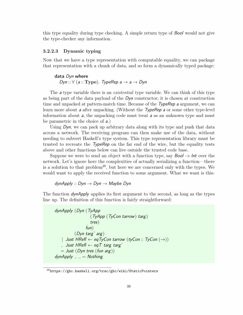
this type equality during type checking. A simple return type of Bool would not givethe type-checker any information.

3.2.2.3 Dynamic typing

Now that we have a type representation with computable equality, we can packagethat representation with a chunk of data, and so form a dynamically typed package:

data Dyn whereDyn :: ∀ (a :: Type). TypeRep a→ a→ Dyn

The a type variable there is an existential type variable. We can think of this typeas being part of the data payload of the Dyn constructor; it is chosen at constructiontime and unpacked at pattern-match time. Because of the TypeRep a argument, we canlearn more about a after unpacking. (Without the TypeRep a or some other type-levelinformation about a, the unpacking code must treat a as an unknown type and mustbe parametric in the choice of a.)

Using Dyn, we can pack up arbitrary data along with its type and push that dataacross a network. The receiving program can then make use of the data, withoutneeding to subvert Haskell’s type system. This type representation library must betrusted to recreate the TypeRep on the far end of the wire, but the equality testsabove and other functions below can live outside the trusted code base.

Suppose we were to send an object with a function type, say Bool → Int over thenetwork. Let’s ignore here the complexities of actually serializing a function—thereis a solution to that problem20, but here we are concerned only with the types. Wewould want to apply the received function to some argument. What we want is this:

dynApply :: Dyn→ Dyn→ Maybe Dyn

The function dynApply applies its first argument to the second, as long as the typesline up. The definition of this function is fairly straightforward:

dynApply (Dyn (TyApp(TyApp (TyCon tarrow) targ)tres)

fun)(Dyn targ’ arg)

| Just HRefl ← eqTyCon tarrow (tyCon :: TyCon (→)), Just HRefl ← eqT targ targ’= Just (Dyn tres (fun arg))

dynApply = Nothing

20https://ghc.haskell.org/trac/ghc/wiki/StaticPointers

38

We first match against the expected type structure—the first Dyn argument must be afunction type. We then confirm that the TyCon tarrow is indeed the representation for(→) (the construct tyCon ::TyCon (→) retrieves the compiler-generated representationfor (→)) and that the actual argument type matches the expected argument type. Ifeverything is good so far, we succeed, applying the function in fun arg .

3.2.2.4 Conclusion

Heterogeneous equality is necessary throughout this example. It first is necessary in thedefinition of eqT . In the TyApp case, we compare a1 to a2 . If we had only homogeneousequality, it would be necessary that the types represented by a1 and a2 be of the samekind. Yet, we can’t know this here! Even if the types represented by TyApp a1 b1 andTyApp a2 b2 have the same kind, it is possible that a1 and a2 would not. (For example,maybe the type represented by a1 has kind Type→ Type and the type representedby a2 has kind Bool → Type.) With only homogeneous equality, we cannot evenwrite an equality function over this form of type representation. The problem repeatsitself in the definition of dynApply , when calling eqTyCon tarrow TArrow . The call toeqT in dynApply , on the other hand, could be homogeneous, as we would know atthat point that the types represented by targ and targ’ are both of kind Type.

In today’s Haskell, the lack of heterogeneous equality means that dynApply mustrely critically on unsafeCoerce. With heterogeneous equality, dynApply can remainsafely outside the trusted code base.

3.2.3 Algebraic effects

Brady [8] describes an approach to the challenge of embedding side effects into a pure,functional language. His approach is to use composable algebraic effects, implementedas a domain-specific language embedded in Idris [9], a full spectrum dependently typedlanguage. This technique is meant to contrast with Haskell’s monad transformers [55].Brady’s library, Effects, is translatable directly into Dependent Haskell. With heavyuse of singletons, all of the code described in the original paper is even implementablein GHC 8.21

3.2.3.1 Example 1: an simple expression interpreter

To give you an idea of the power and flexibility of the algebraic effects approach,let’s look at a function that interprets a simple expression language.22 Here is theexpression AST:

data Expr = Val Nat | Add Expr Expr | Var String | Random Nat

21The code is available at https://github.com/goldfirere/thesis/tree/master/effects. Itdoes not compile with GHC 8.0.1 due to a small implementation bug. The fix is in the latestdevelopment version of GHC and may be available in GHC 8.0.2.

22This example is adapted from Brady [8, Section 2.1.3].

39

Expressions can contain literal numbers,23 addition, variable references, and naturalsrandomly generated up to some specified limit. In the version we will consider, theinterpreter is instrumented to print out the value of every random number generated.Thus the interpreter needs four different effectful capabilities: the ability to deal witherrors (in case a named variable does not exist), the ability to write output, access toa pseudo-random number generator, and an ambient environment of defined variables.This ambient environment has type Vars, an association list mapping variable namesto their values:

type Vars = [(String ,Nat)]

With all that in mind, here is the evaluator:

eval :: Handler StdIO e⇒ Expr → Eff e ’[EXCEPTION String , STDIO,RND, STATE Vars ] Nat

eval (Val x) = return xeval (Var x) = do vs ← get

case lookup x vs ofNothing → raise ("Unknown var: " ++ x)Just val → return val

eval (Add l r) = (+) 〈$〉 eval l 〈∗〉 eval reval (Random upper) = do num← rndNat 0 upper

putStrLn ("Random value: " ++ show num)return num

Let’s first look at the type of eval , with our goal being a general understanding ofwhat this technique brings us, not working out all the details.

The return type of this function is a specialization of Eff , a type defined by theEffects library. Eff is not a monad; the use of do-notation in the code in this section isenabled by the GHC extension RebindableSyntax. With RebindableSyntax, GHCuses whatever symbols are in scope to implement various features. In our case, Effectsdefines >> and >>= operators which work over Eff .

Eff takes three parameters: an underlying effect handler e, a type-level list ofcapabilities, and the return type of the computation. The underlying effect handlermust be able to handle read and write commands. We would generally expect this tobe IO, but an environment with an input list of strings and an output list of stringscould be used to model I/O in a pure environment. The list of capabilities is betterviewed as a set, as the order in this list is immaterial. Fancy footwork done by thetypes of the operations provided by the capabilities (like get or rndNat) looks up thecapability in the list, regardless of order.

23I have restricted this and other examples to work with naturals only. This restriction is in placesolely to play nicely with the use of singletons to translate the Idris library into a form compatiblewith GHC 8. In a full Dependent Haskell implementation, this restriction would not be necessary.

40

Once we’ve absorbed the type of eval , its body is rather uninteresting—and that’sexactly the point! We need not lift one capability through another (as must be donewith monad transformers) nor give any indication of how our capabilities are structured.It all just works.

With eval in hand, it is straightforward to write the function that actually canevaluate an expression:

runEval :: Vars → Expr → IO NatrunEval env expr = run (() :> () :> 123 :> env :> Empty) (eval expr)

The first argument to the Effects library function run is an environment of resources,where each resource is associated with a capability. While the order of capabilities doesnot matter in the body of eval , its order must match up with the order of resourcesgiven when running an Eff computation. In this case, the EXCEPTION String andSTDIO capabilities have no associated resource (the entries in the environment areboth ()). The RND capability uses a random generation seed (123 in our case), andthe STATE Vars needs the initial state, passed as a parameter to runEval .

Having defined all of the above, we can now observe this interaction:

λ> runEval [("x", 3)] (Var "x" ‘Add ‘ Random 12)Random value: 14

In this output, the 4 at the end is the result of evaluating the expression, which addsthe value of "x", 3, to the pseudo-random number 1.

3.2.3.2 Automatic lifting

In the example above, we can use the STATE capability with its get accessor, despitethe fact that STATE is buried at the bottom of the list of capabilities. This is done byget’s rather clever type:

get :: Π (prf :: SubList ’[STATE x ] xs).prf ∼ ’findSubListProof ’[STATE x ] xs

⇒ EffM m xs (UpdateWith ’[STATE x ] xs prf ) x

The function get takes in a proof that ’[STATE x ] xs is a sublist of xs, the list ofcapabilities in the result type. (EffM is a generalization of Eff that allows for thecapabilities to change during a computation. It lists the “before” capabilities and the“after” capabilities. Eff is just a type synonym for EffM with both lists the same.)Despite taking the proof in as an argument, get requires that the proof be the onefound by the findSubListProof function. In this way, the calling code does not need towrite the proof by hand; it can be discovered automatically. However, note that the

41

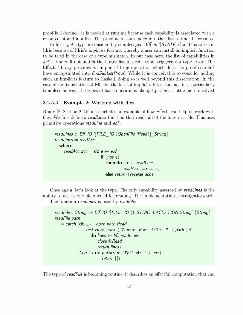
proof is Π-bound—it is needed at runtime because each capability is associated with aresource, stored in a list. The proof acts as an index into that list to find the resource.

In Idris, get’s type is considerably simpler: get ::Eff m ’[STATE x ] x . This works inIdris because of Idris’s implicits feature, whereby a user can install an implicit functionto be tried in the case of a type mismatch. In our case here, the list of capabilities inget’s type will not match the larger list in eval ’s type, triggering a type error. TheEffects library provides an implicit lifting operation which does the proof search Ihave encapsulated into findSubListProof . While it is conceivable to consider addingsuch an implicits feature to Haskell, doing so is well beyond this dissertation. In thecase of my translation of Effects, the lack of implicits bites, but not in a particularlytroublesome way; the types of basic operations like get just get a little more involved.

3.2.3.3 Example 2: Working with files

Brady [8, Section 2.2.5] also includes an example of how Effects can help us work withfiles. We first define a readLines function that reads all of the lines in a file. This usesprimitive operations readLine and eof .

readLines :: Eff IO ’[FILE_IO (OpenFile ’Read)] [String ]readLines = readAcc [ ]wherereadAcc acc = do e ← eof

if (not e)then do str ← readLine

readAcc (str : acc)else return (reverse acc)

Once again, let’s look at the type. The only capability asserted by readLines is theability to access one file opened for reading. The implementation is straightforward.

The function readLines is used by readFile:

readFile :: String → Eff IO ’[FILE_IO (), STDIO,EXCEPTION String ] [String ]readFile path

= catch (do ← open path Readtest Here (raise ("Cannot open file: " ++ path)) $do lines ← lift readLines

close @Readreturn lines)

(λerr → do putStrLn ("Failed: " ++ err)return [ ])

The type of readFile is becoming routine: it describes an effectful computation that can

42

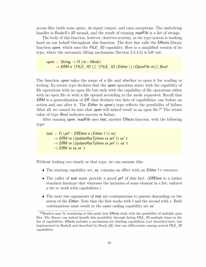
access files (with none open), do input/output, and raise exceptions. The underlyinghandler is Haskell’s IO monad, and the result of running readFile is a list of strings.

The body of this function, however, deserves scrutiny, as the type system is workinghard on our behalf throughout this function. The first line calls the Effects libraryfunction open, which uses the FILE_IO capability. Here is a simplified version of itstype, where the automatic lifting mechanism (Section 3.2.3.2) is left out:

open :: String → Π (m :: Mode)→ EffM e ’[FILE_IO ()] ’[FILE_IO (Either () (OpenFile m))] Bool

The function open takes the name of a file and whether to open it for reading orwriting. Its return type declares that the open operation starts with the capability offile operations with no open file but ends with the capability of file operations eitherwith no open file or with a file opened according to the mode requested. Recall thatEffM is a generalization of Eff that declares two lists of capabilities: one before anaction and one after it. The Either in open’s type reflects the possibility of failure.After all, we cannot be sure that open will indeed result in an open file.24 The returnvalue of type Bool indicates success or failure.

After running open, readFile uses test, another Effects function, with the followingtype:

test :: Π (prf :: EffElem e (Either l r) xs)→ EffM m (UpdateResTyImm xs prf l) xs’ t→ EffM m (UpdateResTyImm xs prf r) xs’ t→ EffM m xs xs’ t

Without looking too closely at that type, we can surmise this:

• The starting capability set, xs, contains an effect with an Either l r resource.

• The caller of test must provide a proof prf of this fact. (EffElem is a ratherstandard datatype that witnesses the inclusion of some element in a list, tailoreda bit to work with capabilities.)

• The next two arguments of test are continuations to pursue depending on thestatus of the Either . Note that the first works with l and the second with r . Bothcontinuations must result in the same ending capability set xs’ .

24Readers may be wondering at this point how Effects deals with the possibility of multiple openfiles. The library can indeed handle this possibility through listing FILE_IO multiple times in thelist of capabilities. Effects includes a mechanism for labeling capabilities (not described here, butimplemented in Haskell and described by Brady [8]) that can differentiate among several FILE_IOcapabilities.

43

• The test operator itself takes the capability set from xs to xs’ .

In our case, test is meant to check the Either () (OpenFile ’Read), stored in the firstcapability. (Here is the proof that the capability we seek is first in the list.) If theEither is Left, raise an exception. Otherwise, we know that the open succeeded, andthe inner do block can work with a capability FILE_IO (OpenFile ’Read).

The inner do block runs readLines, using lift because the type of readLines assumesonly the one FILE_IO capability, and readFile has more than just that. The sameautomatic proof search facility described earlier works with explicit lifts.

The use of close here is again interesting, because omitting it would be a typeerror. Here is close’s type (again, eliding the lifting machinery):

close :: ∀ m e. EffM e ’[FILE_IO (OpenFile m)] ’[FILE_IO ()] ()

It takes an OpenFile and closes it. Forgetting this step would be a type error becausetest requires that both paths result in the same set of capabilities. The failure pathfrom test has no open files at the end, and so the success path must also end with noopen files. The type of close achieves this.

A careful reader will note that we have to specify the Read invisible parameterto close. This is necessary to support the automatic lifting mechanism. Withoutknowing that it is searching for FILE_IO (OpenFile Read), it gets quite confused;looking for FILE_IO (OpenFile m) is just not specific enough. It is conceivable thatthis restriction could be lifted with a cleverer automatic lifting mechanism or atype-checker plugin [22, 38].

All of the code described above is wrapped in a catch in order to deal with anypossible exception; catch is not intricately typed and does not deserve further studyhere.

Having written readFile, we can now use it:

printFile :: FilePath→ IO ()printFile filepath

= do ls ← run (() :> () :> () :> Empty) (readFile filepath)mapM_ putStrLn ls

The return type of printFile is just the regular Haskell IO monad. Due to the wayGHC’s RebindableSyntax extension works, printFile must be written in a separatemodule from the code above in order to access the usual monadic meaning of do.

This example has shown us how the Effects not only makes it easy to mix andmatch different effects without the quadratic code cost of monad transformers, butit also helps us remember to release resources. Forgetting to release a resource hasbecome a type error.

44

3.2.3.4 Example 3: an interpreter for a well-typed imperative language

The final example with Effects is also the culminating example by Brady [8, Section 4]:an interpreter for an imperative language with mutable state. The goal of presentingthis example is simply to show that Effects scales to ever more intricate types, evenin its translation to Haskell. Accordingly, I will be suppressing many details in thispresentation. The curious can read the full source code online.25

This language, Imp, contains both expressions and statements:

data Ty = ... -- types in ImpinterpTy :: Ty → Type -- consider a Ty as a real Haskell Typedata Expr :: ∀ n. Vec Ty n→ Ty → Type where ...data Imp :: ∀ n. Vec Ty n→ Ty → Type where ...

Following the implementation in Idris, my translation uses a deep embedding for thetypes, using the datatype Ty instead of Haskell’s types. This is purely a design choice;using Haskell’s types works just as well.26

Expressions and statements (the datatype Imp) are parameterized over a vectorof types given to de Bruijn-indexed variables. Both expressions and statements alsoproduce an output value, included in their types above. Thus, an expression of typeExpr g t has type t in the typing context g .

Let’s focus on the statement form that introduces a new, mutable variable:

data Imp :: ∀ n. Vec Ty n→ Ty → Type whereLet :: ∀ t g u. Expr g t → Imp (t :& g) u → Imp g u...

The variable, of type t, is given an initial value by evaluating the Expr g t. The bodyof the Let is an Imp (t :& g) u—that is, a statement of type u in a context extendedby t. (The operator :& is the cons operator for Vec , here.)

Here is how such a statement is interpreted:25https://github.com/goldfirere/thesis/blob/master/effects/Sec4.hs26Interestingly, the use of a deep embedding in my implementation means that I have to label

interpTy as injective [86]. Otherwise, type inference fails. Idris’s type inference algorithm mustsimilarly use injectivity to accept this program.

45

interp :: ∀ g t. Imp g t → Eff IO ’[STDIO,RND, STATE (Vars g)] ( ’interpTy t)interp (Let @t’ e sc)

= do e’ ← lift (eval e)vars ← get @(Vars g)putM @(Vars g) (e’ :ˆ vars)res ← interp sc( :ˆ vars’)← get @(Vars (t’ :& g))putM @(Vars (t’ :& g)) vars’return res

I will skip over most of the details here, making only these points:

• It is necessary to use the @ invisibility override (Section 4.2.3.1) several timesso that the automatic lifting mechanism knows what to look for. Alternatives tothe approach seen here include using explicit labels on capabilities (see Brady [8,Section 2.1.2]), writing down the index of the capability desired, or implementinga type-checker plugin to help do automatic lifting.

• The putM function (an operation on STATE ) changes the type of the storedstate. In this case, the stored state is a vector that is extended with the newvariable. We must, however, remember to restore the original state, as otherwisethe final list of capabilities would be different than the starting list, a violation ofinterp’s type. (Recall that Eff , in interp’s type, requires the same final capabilityset as its initial capability set.)

• The eval function (elided from this text) uses a smaller set of capabilities. Itsuse must be lifted.

Despite the ever fancier types seen in this example, Haskell still holds up. Therequirement to specify the many invisible arguments (such as @(Vars g)) is indeedregrettable; however, I feel confident that some future work could resolve this painpoint.

3.2.3.5 Conclusion

The Effects library is a major achievement in Idris and shows some of the powerof dependent types for practical programming. I have shown here that this librarycan be ported to Dependent Haskell, where it remains just as useful. Perhaps asDependent Haskell is adopted, more users will prefer to use this approach over monadtransformers.

46

3.3 Why Haskell?There already exist several dependently typed languages. Why do we need another?This section presents several reasons why I believe the work described in this disserta-tion will have impact.

3.3.1 Increased reach

Haskell currently has some level of adoption in industry.27 Haskell is also used as thelanguage of choice in several academic programs used to teach functional programming.There is also the ongoing success of the Haskell Symposium. These facts all indicatethat the Haskell community is active and sizeable. If GHC, the primary Haskellcompiler, offers dependent types, more users will have immediate access to dependenttypes than ever before.

The existing dependently typed languages were all created, more or less, as play-grounds for dependently typed programming. For a programmer to choose to write herprogram in an existing dependently typed language, she would have to be thinkingabout dependent types (or the possibility of dependent types) from the start. However,Haskell is, first and foremost, a general purpose functional programming language. Aprogrammer might start his work in Haskell without even being aware of dependenttypes, and then as his experience grows, decide to add rich typing to a portion of hisprogram.

With the increased exposure GHC would offer to dependent types, the academiccommunity will gain more insight into dependent types and their practical use inprograms meant to get work done.

3.3.2 Backward-compatible type inference

Working in the context of Haskell gives me a stringent, immovable constraint: my workmust be backward compatible. In the new version of GHC that supports dependenttypes, all current programs must continue to compile. In particular, this means thattype inference must remain able to infer all the types it does today, including typesfor definitions with no top-level annotation. Agda and Idris require a top-level typeannotation for every function; Coq uses inference where possible for top-level definitionsbut is sometimes unpredictable. Furthermore, Haskellers expect the type inferenceengine to work hard on their behalf; they wish to rarely rely on manual provingtechniques.

27At the time of writing, https://wiki.haskell.org/Haskell_in_industry lists 81 companieswho use Haskell to some degree. That page, of course, is world-editable and is not authoritative.However, I am personally aware of Haskell’s (growing) use in several industrial settings, and Ihave seen quite a few job postings looking for Haskell programmers in industry. For example, seehttp://functionaljobs.com/jobs/search/?q=haskell.

47

The requirement of backward compatibility keeps me honest in my design of typeinference—I cannot cheat by asking the user for more information. The technicalcontent of this statement is discussed in Chapter 6 by comparison with the work ofVytiniotis et al. [99] and Eisenberg et al. [33]. See Sections 6.8.2 and 6.8.3. A furtheradvantage of working in Haskell is that the type inference of Haskell is well studied inthe literature. This dissertation continues this tradition in Chapter 6.

3.3.3 No termination or totality checking

Many dependently typed languages today strive to be proof systems as well asprogramming languages. These care deeply about totality: that all pattern matchesconsider all possibilities and that every function can be proved to terminate. Coqdoes not accept a function until it is proved to terminate. Agda behaves likewise,although the termination checker can be disabled on a per-function basis. Idrisembraces partiality, but then refuses to evaluate partial functions during type-checking.Dependent Haskell, on the other hand, does not care about totality.

Dependent Haskell emphatically does not strive to be a proof system. In a proofsystem, whether or not a type is inhabited is equivalent to whether or not a propositionholds. Yet, in Haskell, all types are inhabited, by ⊥ and other looping terms, at aminimum. Even at the type level, all kinds are inhabited by the following type family,defined in GHC’s standard library:

type family Any :: k -- no instances

The type family Any can be used at any kind, and so inhabits all kinds.Furthermore, Dependent Haskell has the Type :Type axiom, meaning that instead

of having an infinite hierarchy of universes characteristic of Coq, Agda, and Idris,Dependent Haskell has just one universe, which contains itself. It is well known thatself-containment of this form leads to logical inconsistency by enabling the constructionof a looping term [36], but I am unbothered by this—Haskell has many other loopingterms, too! (See Section 4.4.1 for more discussion on this point.) By allowing ourselvesto have Type:Type, the type system is much simpler than in systems with a hierarchyof universes.

There are two clear downsides of the lack of totality:

• What appears to be a proof might not be. Suppose we need to prove that type τequals type σ in order to type-check a program. We can always use ⊥ :: τ :≈:σto prove this equality, and then the program will type-check. The problem willbe discovered only at runtime. Another way to see this problem is that equalityproofs must be run, having an impact on performance. However, note that wecannot use the bogus equality without evaluating it; there is no soundness issue.

This drawback is indeed serious, and important future work includes designingand implementing a totality checker for Haskell. (See the work of Vazou et al.

48

[94] for one approach toward this goal. Recent work by Karachalias et al. [51]is another key building block.) Unlike in other languages, though, the totalitychecker would be chiefly used in order to optimize away proofs, rather than tokeep the language safe. Once the checker is working, we could also add compilerflags to give programmers compile-time warnings or errors about partial functions,if requested.

• Lack of termination in functions used at the type level might conceivably causeGHC to loop. This is not a great concern, however, because the loop is directlycaused by a user’s type-level program. In practice, GHC counts steps it uses inreducing types and reports an error after too many steps are taken. The usercan, via a compiler flag, increase the limit or disable the check.

The advantages to the lack of totality checking are that Dependent Haskell issimpler for not worrying about totality. It is also more expressive, treating partialfunctions as first-class citizens.

3.3.4 GHC is an industrial-strength compiler

Hosting dependent types within GHC is likely to reveal new insights about dependenttypes due to all of the features that GHC offers. Not only are there many surfacelanguage extensions that must be made to work with dependent types, but the backend must also be adapted. A dependently typed intermediate language must, forexample, allow for optimizations. Working in the context of an industrial-strengthcompiler also forces the implementation to be more than just “research quality,” butready for a broad audience.

3.3.5 Manifest type erasure properties

A critical property of Haskell is that it can erase types. Despite all the machineryavailable in Haskell’s type system, all type information can be dropped during compila-tion. In Dependent Haskell, this does not change. However, dependent types certainlyblur the line between term and type, and so what, precisely, gets erased can bedifficult to discern. Dependent Haskell, in a way different from other dependentlytyped languages, makes clear which arguments to functions (and data constructors)get erased. This is through the user’s choice of relevant vs. irrelevant quantifiers, asexplored in Section 4.2.2. Because erasure properties are manifestly available in types,a performance-conscious user can audit a Dependent Haskell program and see exactlywhat will be removed at runtime.

It is possible that, with practice, this ability will become burdensome, in that theuser has to figure out what to keep and what to discard. Idris’s progress toward typeerasure analysis [10, 90] may benefit Dependent Haskell as well.

49

3.3.6 Type-checker plugin support

Recent versions of GHC allow type-checker plugins, a feature that allows end users towrite a custom solver for some domain of interest. For example, Gundry [38] uses aplugin to solve constraints arising from using Haskell’s type system to check that aphysical computation respects units of measure. As another example, Diatchki [22] haswritten a plugin that uses an SMT solver to work out certain numerical constraintsthat can arise using GHC’s type-level numbers feature.

Once Haskell is equipped with dependent types, the need for these plugins willonly increase. However, because GHC already has this accessible interface, the work ofdeveloping the best solvers for Dependent Haskell can be distributed over the Haskellcommunity. This democratizes the development of dependently typed programs andspurs innovation in a way a centralized development process cannot.

3.3.7 Haskellers want dependent types

The design of Haskell has slowly been marching toward having dependent types.Haskellers have enthusiastically taken advantage of the new features. For example, over1,000 packages published at hackage.haskell.org use type families [86]. Anecdotally,Haskellers are excited about getting full dependent types, instead of just fakingthem [30, 59, 60]. Furthermore, with all of the type-level programming features thatexist in Haskell today, it is a reasonable step to go to full dependency.

50

Chapter 4

Dependent Haskell

This chapter provides an overview of Dependent Haskell. I will review the new featuresof the type language (Section 4.1), introduce the small menagerie of quantifiersavailable in Dependent Haskell (Section 4.2), explain pattern matching in the presenceof dependent types (Section 4.3), and conclude the chapter by discussing severalfurther points of interest in the design of the language.

There are many examples throughout this chapter, building on the followingdefinitions:

-- Length-indexed vectors, from Section 3.1.1data Nat = Zero | Succ Natdata Vec :: Type→ Nat → Type whereNil :: Vec a ’Zero(:>) :: a→ Vec a n→ Vec a ( ’Succ n)

infixr 5 :>

-- Propositional equality, from Section 2.4data a :∼: b whereRefl :: a :∼: a-- Heterogeneous lists, indexed by the list of types of elements

data HList :: [Type ]→ Type whereHNil :: HList ’[ ](:::) :: h→ HList t → HList (h ’: t)

infixr 5 :::

4.1 Dependent Haskell is dependently typedThe most noticeable change when going from Haskell to Dependent Haskell is that thelatter is a full-spectrum dependently typed language. Expressions and types intermix.This actually is not too great a shock to the Haskell programmer, as the syntax of

51

Haskell expressions and Haskell types is so similar. However, by utterly dropping thedistinction, Dependent Haskell has many more possibilities in types, as seen in thelast chapter.

No distinction between types and kinds The kind system of GHC 7.10 andearlier is described in Section 2.3. It maintained a distinction between types, whichclassify terms, and kinds, which classify types. Yorgey et al. [107] enriched the languageof kinds, allowing for some types to be promoted into kinds, but it did not mix thetwo levels.

My prior work [105] goes one step further than Yorgey et al. [107] and does mergetypes with kinds by allowing non-trivial equalities to exist among kinds. See my priorwork for the details; this feature does not come through saliently in this dissertation,as I never consider any distinction between types and kinds. It is this work that isimplemented and released in GHC 8. Removing the distinction between types andkinds has opened up new possibilities to the Haskell programmer. Below are briefexamples of these new capabilities:

• Explicit kind quantification. Previously, kind variables were all quantified implic-itly. GHC 8 allows explicit kind quantification:

data Proxy k (a :: k) = Proxy-- NB: Proxy takes both kind and type arguments

f :: ∀ k (a :: k). Proxy k a→ ()

• Kind-indexed GADTs. Previously, a GADT could vary the return types ofconstructors only in its type variables, never its kind variables; this restriction islifted. Here is a contrived example:

data G (a :: k) whereMkG1 :: G IntMkG2 :: G Maybe

Notice that Int and Maybe have different kinds, and thus that the instantiationof the G ’s k parameter is non-uniform between the constructors. Some recentprior work [75] explores applying a kind-indexed to enabling dynamic typeswithin Haskell.

• Universal promotion. As outlined by Yorgey et al. [107, Section 3.3], only sometypes were promoted to kinds in GHC 7.10 and below. In contrast, GHC 8 allowsall types to be used in kinds. This includes type synonyms and type families,allowing computation in kinds for the first time.

52

• GADT constructors in types. A constructor for a GADT packs an equalityproof, which is then exposed when the constructor is matched against. BecauseGHC 7.10 and earlier lacked informative equality proofs among kinds, GADTconstructors could not be used in types. (They were simply not promoted.)However, with the rich kind equalities permitted in GHC 8, GADT constructorscan be used freely in types, and type families may perform GADT patternmatching.

Expression variables in types Dependent Haskell obviates the need for mostclosed type families by allowing the use of ordinary functions directly in types. BecauseHaskell has a separate term-level namespace from its type-level namespace, any term-level definition used in a type must be prefixed with a ’ mark. This expands the useof a ’ mark to promote constructors as initially introduced by Yorgey et al. [107]. Forexample:

(+) :: Nat → Nat → NatZero + m = mSucc n + m = Succ (n + m)

append :: Vec a n→ Vec a m→ Vec a (n ’+m)append Nil v = vappend (h :> t) v = h :> (append t v)

Note that this ability does not eliminate all closed type families, as term-level functiondefinitions cannot use non-linear patterns, nor can they perform unsaturated matches(see Section 5.1.1.2).

Type names in terms It is sometimes necessary to go the other way and mentiona type when writing something that syntactically appears to be a term. For the samereasons we need ’ when using a term-level name in a type, we use ˆ to use a type-levelname in a term. A case in point is the code appearing in Section 3.1.3.2.

Pattern matching in types It is now possible to use case directly in a type:

tailOrNil :: Vec a n→ Vec a (case n of’Zero → ’Zero’Succ n’ → n’)

tailOrNil Nil = NiltailOrNil ( :> t) = t

53

Anonymous functions in types Types may now include λ-expressions:

eitherize :: HList types → HList ( ’map (λty → Either ty String) types)eitherize HNil = HNileitherize (h ::: t) = Left h ::: eitherize t

Other expression-level syntax in types Having merged types and expressions,all expression-level syntax is now available in types (for example, do-notation, letbindings, even arrows [46]). From a compilation standpoint, supporting these featuresis actually not a great challenge (once we have Chapters 5 and 6 implemented); itrequires only interleaving type-checking with desugaring.28 When a type-level useof elaborate expression-level syntax is encountered, we will need to work with thedesugared version, hence the interleaving.

4.2 QuantifiersBeyond simply allowing old syntax in new places, as demonstrated above, DependentHaskell also introduces new quantifiers that allow users to write a broader set offunctions than was previously possible. Before looking at the new quantifiers ofDependent Haskell, it is helpful to understand the several axes along which quantifierscan vary in the context of today’s Haskell.

In Haskell, a quantifier is a type-level operator that introduces the type of anabstraction, or function. In Dependent Haskell, there are four essential propertiesof quantifiers, each of which can vary independently of the others. To understandthe range of quantifiers that the language offers, we must go through each of theseproperties. In the text that follows, I use the term quantifiee to refer to the argumentquantified over. The quantifier body is the type “to the right” of the quantifier. Thequantifiers introduced in this section are summarized in Figure 4.1 on page 59.

4.2.1 Dependency

A quantifiee may be either dependent or non-dependent. A dependent quantifiee maybe used in the quantifier body; a non-dependent quantifiee may not.

Today’s Haskell uses ∀ for dependent quantification, as follows:

id :: ∀ a. a→ a

In this example, a is the quantifiee, and a→ a is the quantifier body. Note that thequantifiee a is used in the quantifier body.

28GHC currently type-checks the Haskell source directly, allowing it to produce better errormessages. Only after type-checking and type inference does it convert Haskell source into its internallanguage, the process called desugaring.

54

The normal function arrow (→) is an example of a non-dependent quantifier.Consider the predecessor function:

pred :: Int → Int

The Int quantifiee is not named in the type, nor is it mentioned in the quantifier body.In addition to ∀, Dependent Haskell adds a new dependent quantifier, Π. The only

difference between Π and ∀ is that Π-quantifiee is relevant, as we’ll explore next.

4.2.2 Relevance

A quantifiee may be either relevant or irrelevant. A relevant quantifiee may be usedanywhere in the function quantified over; an irrelevant quantifiee may be used only inirrelevant positions—that is, as an irrelevant argument to other functions or in typeannotations. Note that relevance talks about usage in the function quantified over,not the type quantified over (which is covered by the dependency property).

Relevance is very closely tied to type erasure. Relevant arguments in terms areprecisely those arguments that are not erased. However, the relevance property appliesequally to type-level functions, where erasure does not make sense, as all types areerased. For gaining an intuition about relevance, thinking about type erasure is a verygood guide.

Today’s Haskell uses (→) for relevant quantification. For example, here is the bodyof pred :

pred x = x − 1

Note that x , a relevant quantifiee, is used in a relevant position on the right-handside. Relevant positions include all places in a term or type that are not within atype annotation, other type-level context, or irrelevant argument context, as will bedemonstrated in the next example.

Today’s Haskell uses ∀ for irrelevant quantification. For example, here is the bodyof id (as given a type signature above):

id x = (x :: a)

The type variable a is the irrelevant quantifiee. According to Haskell’s scoped typevariables, it is brought into scope by the ∀ a in id ’s type annotation. (It could also bebrought into scope by using a in a type annotation on the pattern x to the left of the=.) Although a is used in the body of id , it is used only in an irrelevant position, inthe type annotation for x . It would violate the irrelevance of ∀ for a to be used outsideof a type annotation or other irrelevant context. As functions can take irrelevantarguments, irrelevant contexts include these irrelevant arguments.

Dependent Haskell adds a new relevant quantifier, Π. The fact that Π is bothrelevant and dependent is the very reason for Π’s existence!

55

4.2.3 Visibility

A quantifiee may be either visible or invisible. The argument used to instantiate avisible quantifiee appears in the Haskell source; the argument used to instantiate aninvisible quantifiee is elided.

Today’s Haskell uses (→) for visible quantification. That is, when we pass anordinary function an argument, the argument is visible in the Haskell source. Forexample, the 3 in pred 3 is visible.

On the other hand, today’s ∀ and (⇒) are invisible quantifiers. When we callid True, the a in the type of id is instantiated at Bool , but Bool is elided in the callid True. During type inference, GHC uses unification to discover that the correctargument to use for a is Bool .

Invisible arguments specified with (⇒) are constraints. Take, for example, show ::∀ a. Show a ⇒ a → String . The show function properly takes 3 arguments: the∀-quantified type variable a, the (⇒)-quantified dictionary for Show a (see Section 2.1if this statement surprises you), and the (→)-quantified argument of type a. However,we use show as, say, show True, passing only one argument visibly. The ∀ a argumentis discovered by unification to be Bool , but the Show a argument is discovered usinga different mechanism: instance solving and lookup. (See the work of Vytiniotis et al.[99] for the algorithm used.) We thus must be aware that invisible arguments may usedifferent mechanisms for instantiation.

Dependent Haskell offers both visible and invisible forms of ∀ and Π; the invisibleforms instantiate only via unification. Dependent Haskell retains, of course, the invisiblequantifier (⇒), which is instantiated via instance lookup and solving. Finally, notethat visibility is a quality only of source Haskell. All arguments are always “visible” inPico.

It may be helpful to compare Dependent Haskell’s treatment of visibility to thatin other languages; see Section 8.6.

4.2.3.1 Visibility overrides

It is often desirable when using rich types to override a declared visibility specification.That is, when a function is declared to have an invisible parameter a, a call site maywish to instantiate a visibly. Conversely, a function may declare a visible parameterb, but a caller knows that the choice for b can be discovered by unification and sowishes to omit it at the call site.

Instantiating invisible parameters visibly Dependent Haskell adopts the @ . . .syntax of Eisenberg et al. [33] to instantiate any invisible parameter visibly, whetherit is a type or not. Continuing our example with id , we could write id @Bool Trueinstead of id True. This syntax works in patterns, expressions, and types. In patterns,the choice of @ conflicts with as-patterns, such as using the pattern list@(x :xs) to bindlist to the whole list while pattern matching. However, as-patterns are almost always

56

written without whitespace. I thus use the presence of whitespace before the @ tosignal the choice between an as-pattern and a visibility override.29 Dictionaries cannotbe named in Haskell, so this visibility override skips over any constraint arguments.

Omitting visible parameters The function replicate :: Π (n ::Nat)→ a→ Vec a nfrom Section 3.1.1.3 creates a length-indexed vector of length n, where n is passedin as the first visible argument. (The true first argument is a, which is invisible andelided from the type.) However, the choice for n can be inferred from the context. Forexample:

theSimons :: Vec String 2theSimons = replicate 2 "Simon"

In this case, the two uses of 2 are redundant. We know from the type signature thatthe length of theSimons should be 2. So we can omit the visible parameter n whencalling replicate:

theSimons’ :: Vec String 2theSimons’ = replicate "Simon"

The underscore tells GHC to infer the missing parameter via unification.The two overrides can usefully be combined, when we wish to infer the instantiation

of some invisible parameters but then specify the value for some later invisibleparameter. Consider, for example, coerce :: ∀ a b. Coercible a b ⇒ a→ b. In the callcoerce (MkAge 3) (where we have newtype Age = MkAge Int), we can infer the valuefor a, but the choice for b is a mystery. We can thus say coerce @_ @Int (MkAge 3),which will convert MkAge 3 to an Int.

The choice of syntax for omitting visible parameters conflicts somewhat with thefeature of typed holes, whereby a programmer can leave out a part of an expression,replacing it with an underscore, and then get an informative error message about thetype of expression expected at that point in the program. (This is not unlike Agda’ssheds feature or Idris’s metavariables feature.) However, this is not a true conflict, asan uninferrable omitted visible parameter is indeed an error and should be reported;the error report is that of a typed hole. Depending on user feedback, this override ofthe underscore symbol may be hidden behind a language extension or other compilerflag.

29This perhaps-surprising decision based on whitespace is regrettable, but it has company. Thesymbol $ can mean an ordinary, user-defined operator when it is followed by a space but a TemplateHaskell splice when there is no space. The symbol . can mean an ordinary, user-defined operatorwhen it is preceded by a space but indicate namespace resolution when it is not. Introducing theseoddities seems a good bargain for concision in the final language.

57

4.2.4 Matchability

Suppose we know that f a equals g b. What relationship can we conclude aboutthe individual pieces? In general, nothing: there is no way to reduce f a ∼ g b forarbitrary f and g . Yet Haskell type inference must simplify such equations frequently.For example:

class Monad m wherereturn :: a→ m a...

just5 :: Maybe Intjust5 = return 5

When calling return in the body of just5 , type inference must determine how toinstantiate the call to return. We can see that m a (the return type of return) must beMaybe Int. We surely want type inference to decide to set m to Maybe and a to Int!Otherwise, much current Haskell code would no longer compile.

The reason it is sensible to reduce m a ∼ Maybe Int to m ∼ Maybe and a ∼ Intis that all type constructors in Haskell are generative and injective, according to thesedefinitions:

Definition (Generativity). If f and g are generative, then f a ∼ g b implies f ∼ g.30

Definition (Injectivity). If f is injective, then f a ∼ f b implies a ∼ b.

Because these two notions go together so often in the context of Haskell, I introducea new word matchable, thus:

Definition (Matchability). A function f is matchable iff it is generative and injective.

Thus, we say that all type constructors in Haskell are matchable. Note that if fand g are matchable, then f a ∼ g b implies f ∼ g and a ∼ b, as desired.

On the other hand, ordinary Haskell functions are not, in general, matchable.The inability to reduce f a ∼ g b to f ∼ g and a ∼ b for arbitrary functions isprecisely why type families must be saturated in today’s Haskell. If they were allowedto appear unsaturated, then the type inference algorithm could no longer assume thathigher-kinded types are always matchable,31 and inference would grind to a halt.

The solution is to separate out matchable functions from unmatchable ones,classifying each by their own quantifier, as described in my prior work [29].

The difference already exists in today’s Haskell between a matchable arrow and anunmatchable arrow, though this difference is invisible. When we write an arrow in a

30As we see in this definition, generativity is really a relation between pairs of types. We canconsider the type constructors to be a set such that any pair are generative w.r.t. the other. When Italk about a type being generative, it is in relation to this set.

31For example, unifying a b with Maybe Int would no longer have a unique solution.

58

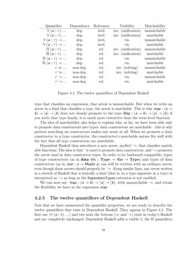
Quantifier Dependency Relevance Visibility Matchability∀ (a :: τ). ... dep. irrel. inv. (unification) unmatchable’∀ (a :: τ). ... dep. irrel. inv. (unification) matchable∀ (a :: τ)→ ... dep. irrel. vis. unmatchable’∀ (a :: τ)→ ... dep. irrel. vis. matchable

Π (a :: τ). ... dep. rel. inv. (unification) unmatchable’Π (a :: τ). ... dep. rel. inv. (unification) matchable

Π (a :: τ)→ ... dep. rel. vis. unmatchable’Π (a :: τ)→ ... dep. rel. vis. matchable

τ ⇒ ... non-dep. rel. inv. (solving) unmatchableτ ’⇒ ... non-dep. rel. inv. (solving) matchableτ → ... non-dep. rel. vis. unmatchableτ ’→ ... non-dep. rel. vis. matchable

Figure 4.1: The twelve quantifiers of Dependent Haskell

type that classifies an expression, that arrow is unmatchable. But when we write anarrow in a kind that classifies a type, the arrow is matchable. This is why map :: (a→b)→ [a ]→ [b ] does not cleanly promote to the type Map :: (a→ b)→ [a ]→ [b ]; ifyou write that type family, it is much more restrictive than the term-level function.

The idea of matchability also helps to explain why, so far, we have been able onlyto promote data constructors into types: data constructors are matchable—this is whypattern matching on constructors makes any sense at all. When we promote a dataconstructor to a type constructor, the constructor’s matchable nature fits well withthe fact that all type constructors are matchable.

Dependent Haskell thus introduces a new arrow, spelled ’→, that classifies match-able functions. The idea is that ’ is used to promote data constructors, and ’→ promotesthe arrow used in data constructor types. In order to be backward compatible, typesof type constructors (as in data Vec :: Type → Nat → Type) and types of dataconstructors (as in Just :: a→ Maybe a) can still be written with an ordinary arrow,even though those arrows should properly be ’→. Along similar lines, any arrow writtenin a stretch of Haskell that is lexically a kind (that is, in a type signature in a type) isinterpreted as ’→ as long as the DependentTypes extension is not enabled.

We can now say ’map :: (a → b) → [a ] → [b ], with unmatchable →, and retainthe flexibility we have in the expression map.

4.2.5 The twelve quantifiers of Dependent Haskell

Now that we have enumerated the quantifier properties, we are ready to describe thetwelve quantifiers that exist in Dependent Haskell. They appear in Figure 4.1. Thefirst one (∀ (a :: t). ...) and two near the bottom (⇒ and →) exist in today’s Haskelland are completely unchanged. Dependent Haskell adds a visible ∀, the Π quantifiers,

59

and matchable versions of everything.32

It is expected that the matchable quantifiers will be a rarity in user code. Thesequantifiers are used to describe type and data constructors, but matchability is assumedin a type or data constructor signature. Beyond those signatures, I don’t imaginemany users will need to write matchable function types. However, there is no reasonto prevent users from writing these, so I have included them in the user-facing design.

The visible ∀ is useful in situations where a type parameter might otherwise beambiguous. For example, suppose F is a non-injective [86] type family and considerthis:

frob :: ∀ a. F a→ F [a ]

This type signature is inherently ambiguous—we cannot know the choice of a evenif we know we want a such that frob :: Int → Bool—and GHC reports an error whenit is written. Suppose that we know we want a particular use of frob to have typeInt → Bool . Even with that knowledge, there is no way to determine how to instantiatea. To fix this problem, we simply make a visible:

frob :: ∀ a→ F a→ F [a ]

Now, any call to frob must specify the choice for a, and the type is no longer ambiguous.A Π-quantified parameter is both dependent (it can be used in types) and relevant

(it can be used in terms). Critically, pattern-matching (in a term) on a Π-quantifiedparameter informs our knowledge about that parameter as it is used in types, a subjectwe explore in the next section.

Lastly, Dependent Haskell omits the non-dependent, irrelevant quantifiers, as anon-dependent, irrelevant quantifiee would not be able to be used anywhere.

4.3 Pattern matchingWe will approach an understanding of pattern matches in stages, working through threeexamples of increasing complexity. All these examples will work over the somewhathackneyed length-indexed vectors for simplicity and familiarity.

32The choice of syntax here is directly due to the work of Gundry [37].

60

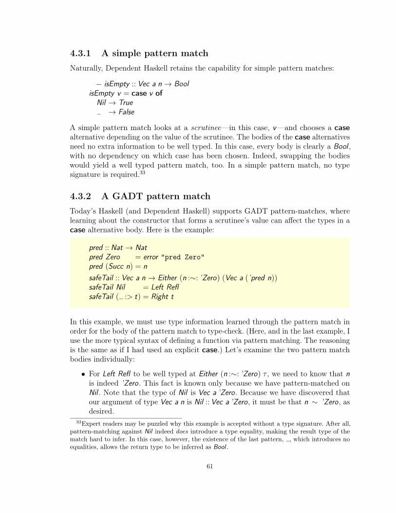
4.3.1 A simple pattern match

Naturally, Dependent Haskell retains the capability for simple pattern matches:

-- isEmpty :: Vec a n→ BoolisEmpty v = case v ofNil → True→ False

A simple pattern match looks at a scrutinee—in this case, v—and chooses a casealternative depending on the value of the scrutinee. The bodies of the case alternativesneed no extra information to be well typed. In this case, every body is clearly a Bool ,with no dependency on which case has been chosen. Indeed, swapping the bodieswould yield a well typed pattern match, too. In a simple pattern match, no typesignature is required.33

4.3.2 A GADT pattern match

Today’s Haskell (and Dependent Haskell) supports GADT pattern-matches, wherelearning about the constructor that forms a scrutinee’s value can affect the types in acase alternative body. Here is the example:

pred :: Nat → Natpred Zero = error "pred Zero"pred (Succ n) = nsafeTail :: Vec a n→ Either (n :∼: ’Zero) (Vec a ( ’pred n))safeTail Nil = Left ReflsafeTail ( :> t) = Right t

In this example, we must use type information learned through the pattern match inorder for the body of the pattern match to type-check. (Here, and in the last example, Iuse the more typical syntax of defining a function via pattern matching. The reasoningis the same as if I had used an explicit case.) Let’s examine the two pattern matchbodies individually:

• For Left Refl to be well typed at Either (n :∼: ’Zero) τ , we need to know that nis indeed ’Zero. This fact is known only because we have pattern-matched onNil . Note that the type of Nil is Vec a ’Zero. Because we have discovered thatour argument of type Vec a n is Nil ::Vec a ’Zero, it must be that n ∼ ’Zero, asdesired.

33Expert readers may be puzzled why this example is accepted without a type signature. After all,pattern-matching against Nil indeed does introduce a type equality, making the result type of thematch hard to infer. In this case, however, the existence of the last pattern, , which introduces noequalities, allows the return type to be inferred as Bool .

61

• For Right t to be well typed at Either τ (Vec a ( ’pred n)) (where t ::Vec a n’ forsome n’), we need to know that n ∼ ’Succ n’ , so that we can simplify ’pred nto ’pred ( ’Succ n’) to n’ . The equality n ∼ ’Succ n’ is exactly what we get bypattern-matching on :>.

Note that I have provided a type signature for safeTail . This is necessary in the eventof a GADT pattern match, because there is no way, in general, to infer the returntype of a pattern match where each branch has a type equality in scope.34

4.3.3 Dependent pattern match

New to Dependent Haskell is the dependent pattern match, shown here:

replicate :: Π n→ a→ Vec a nreplicate Zero = Nilreplicate (Succ n’) x = x :> replicate n’ x

Let’s again consider the function bodies one at a time:

• Its type signature tells us Nil has type Vec a ’Zero. Thus for Nil to be well typedin replicate, we must know that n ∼ ’Zero. We indeed do know this, as we havescrutinized n and found that n is ’Zero.

• For the recursive call to be well typed, we need to know that n ∼ ’Succ n’ ,which is, once again, what we know by the pattern match.

Note the difference between this case of dependent pattern match and the previouscase of GADT pattern match. In GADT pattern matching, the equality assumptionof interest is found by looking at the type of the constructor that we have found. In adependent pattern match, on the other hand, the equality assumption of interest isbetween the scrutinee and the constructor. In our case here, the scrutinized value isnot even of a GADT; Nat is a perfectly ordinary, Haskell98 datatype.

A question naturally comes up in this example: when should we do dependentpattern match and when should we do a traditional (non-dependent) pattern match?A naive answer might be to always do dependent pattern matching, as we can alwaysfeel free to ignore the extra, unused equality if we do not need it. However, this wouldnot work in practice—with an equality assumption in scope, we cannot accurately inferthe return type of a pattern match. Yet this last problem delivers us the solution: usedependent pattern matching only when we know a match’s result type, as propagateddown via a bidirectional type system. (This is much the same way that today’s Haskellallows inference in the presence of higher-rank types [74]. See Section 6.4 for the

34If this last statement is a surprise to you, the introduction of Vytiniotis et al. [99] has a niceexplanation of why this is a hard problem.

62

details.) If we know a result type and do not need the dependent pattern matchequality, no harm is done. On the other hand, if we do not know the result type, thisdesign decision means that dependent pattern matching does not get in the way ofinferring the types of Haskell98 programs.

4.4 DiscussionThe larger syntactic changes to Haskell as it becomes Dependent Haskell are sketchedabove. In addition to these changes, Haskell’s typing rules naturally become muchmore involved. Though a declarative specification remains out of reach, Chapter 6describes (and Appendix D details) the algorithm Bake, which is used to detecttype-correct Dependent Haskell programs. It is important future work to develop amore declarative specification of Dependent Haskell.

This section comments on several topics that affect the design of Dependent Haskell.

4.4.1 Type : Type

Dependent Haskell includes the Type : Type axiom, avoiding the infinite hierarchy ofsorts [57, 80] that appear in other dependently-typed languages. This choice is madesolely to simplify the language. Other languages avoid the Type : Type axiom inorder to remain consistent as a logic. However, to have logical consistency, a languagemust be total. Haskell already has many sources of partiality, so there is little risk inadding one more.

Despite the questionable reputation of the Type : Type axiom, languages withthis feature have been proved type-safe for some time. Cardelli [12] gives a thoroughearly history of the axiom and presents a type-safe language with Type : Type. Giventhe inherent partiality of Haskell, the inclusion of this axiom has little effect on thetheory.

4.4.2 Inferring Π

The discussion of quantifiers in this chapter begs a question: which quantifier is chosenwhen the user has not written any? The answer: →. Despite all of the advances tothe type system that come with Dependent Haskell, the non-dependent, relevant,visible, and unmatchable function type, →, remains the bedrock. In absence of otherinformation, this is the quantifier that will be used.

However, as determined by the type inference process (Chapter 6), an inferredtype might still have a Π in it. For example, if I declare

replicate’ = replicate

without giving a type signature to replicate’ , it should naturally get the same type(which includes a Π) as replicate. Indeed this is what is delivered by Bake, DependentHaskell’s type inference algorithm.

63

On the other hand, the generalized type of the expression λf g x → f (g x)is ∀ a b c . (b → c) → (a → b) → (a → c), the traditional type for functioncomposition, not the much more elaborate type (see Section 6.1) for a dependentlytyped composition function. The more exotic types are introduced only when writtenin by the user.

4.4.3 Roles and dependent types

Integrating dependent types with Haskell’s role mechanism [11] is a challenge, asexplored in some depth in my prior, unpublished work [27]. Instead of addressing thisissue head-on, I am deferring the resolution until we can find a better solution thanwhat was proposed in that prior work. That approach, unworthy of being repeated here,is far too ornate and hard to predict. Instead, I make a simplifying assumption thatall coercions used in types have a nominal role.35 This choice restricts the way Haskellnewtypes can work with dependent types if the coerce function has been used. Aviolation of this restriction (yet to be nailed down, exactly) can be detected after type-checking and does not affect the larger type system. It is my hope that, once the rest ofDependent Haskell is implemented, a solution to this thorny problem will present itself.A leading, unexplored candidate is to have two types of casts: representational andnominal. Currently, all casts are representational; possibly, tracking representationalcasts separately from nominal casts will allow a smoother integration of roles anddependent types than does the ornate approach in my prior work.

4.4.4 Impredicativity, or lack thereof

Despite a published paper [97] and continued attempts at cracking this nut, GHC lackssupport for impredicativity.36 Here, I use the following definitions in my meaning ofimpredicativity, which has admittedly drifted somewhat from its philosophical origins:

Definition (Simple types). A simple type has no constraint, quantification, or de-pendency.

Definition (Impredicativity). A program is impredicative if it requires a non-simpletype to be substituted for a type variable.

Impredicativity is challenging to implement while retaining predictable type infer-ence, essentially because it is impossible to know where to infer invisible arguments—invisible arguments can be hidden behind a type variable in an impredicative typesystem.

Dependent Haskell does not change this state of affairs in any way. In DependentHaskell, just like in today’s Haskell, impredicativity is simply not allowed.

35If you are not familiar with roles, do not fret. Instead, safely skip the rest of this subsection.36There does exist an extension ImpredicativeTypes. However, it is unmaintained, deprecated,

and quite broken.

64

There is a tantalizing future direction here, however: are the restrictions aroundimpredicativity due to invisible binders only? Perhaps. Up until now, it has beenimpossible to have a dependent or irrelevant binder without that binder also beinginvisible. (To wit, ∀ is the invisible, dependent, irrelevant binder of today’s Haskell.)One of the tasks of enhancing Haskell with dependent types is picking apart therelationship among all of the qualities of quantifiers [56]. It is conceivable that thereason impredicativity hinders the predictability of type inference has to do onlywith visibility, allowing arbitrary instantiations of type variables with complex types,as long as they have no invisible binders. Such an idea requires close study beforeimplementing, but by pursuing this idea, we may be able to relax the impredicativityrestriction substantially.

4.4.5 Running proofs

Haskell is a partial language. It has a multitude of ways of introducing a computa-tion that does not reduce to a value: ⊥/error , general recursion, incomplete patternmatches, non-strictly-positive datatypes, baked-in type representations [75], and possi-bly Girard’s paradox [36, 48], among others. This is in sharp contrast to many otherdependently typed language, which are total. (An important exception is Cayenne.See Section 8.3.)

In a total language, if you have a function pf that results in a proof that a ∼ b,you never need to run the function. (Here, I’m ignoring the possibility of multiple,different proofs of equality [91].) By the totality of that language, you are assuredthat pf will always terminate, and thus running pf yields no information.

On the other hand, in a partial language like Haskell, it is always possible that pfdiverges or errors. We are thus required to run pf to make sure that it terminates.This is disappointing, as the only point of running pf is to prove a type equality, andtypes are supposed to be erased. However, the Haskell function pf has two possibleoutcomes: an uninformative (at runtime) proof of type equality, or divergence. Thereseems to be no easy, sound way around this restriction, which will unfortunately havea real effect on the runtimes of dependently typed Haskell programs.37

Despite not having an easy, sound workaround, GHC already comes with an easy,unsound workaround: rewrite rules [73]. A rewrite rule (written with a RULES pragma)instructs GHC to exchange one fragment of a program in its intermediate languagewith another, by pattern matching on the program structure. For example, a user canwrite a rule to change map id to id . To the case in point, a user could write a rulethat changes pf ... to unsafeCoerce Refl . Such a rule would eliminate the possibility ofa runtime cost to the proof. By writing this rule, the user is effectively asserting thatthe proof always terminates.

37Note that running a term like pf is the only negative consequence of Haskell’s partiality. If, say,Agda always ran its proofs, it could be partial, too! This loses logical consistency—and may surpriseusers expecting something that looks like a proof to actually be a proof—but the language wouldremain type safe.

65

4.4.6 Import and export lists

Recall the safeTail example from Section 4.3.2. As discussed in that section, for safeTailto compile, it is necessary to reduce ’pred ( ’Succ n’) to n’ . This reduction requiresknowledge of the details of the implementation of pred . However, if we imagine thatpred is defined in another module, it is conceivable that the author of pred wishes tokeep the precise implementation of pred private—after all, it might change in futureversions of the module. Naturally, hiding the implementation of pred would preventan importing module from writing safeTail , but that should be the library author’sprerogative.

Another way of examining this problem is to recognize that the definition of predencompasses two distinct pieces of information: pred ’s type and pred ’s body. A moduleauthor should have the option of exporting the type without the body.

This finer control is done by a small generalization of the syntax in import andexport lists. If a user includes pred in an import/export list, only the name pred andits type are involved. On the other hand, writing pred(. .) (with a literal (. .) in thesource code) in the import/export list also includes pred ’s implementation. This echoesthe current syntax of using, say, Bool to export only the Bool symbol while Bool(. .)exports Bool with all of its constructors.

4.4.7 Type-checking is undecidable

In order to type-check a Dependent Haskell program, it is sometimes necesary to eval-uate expressions used in types. Of course, these expressions might be non-terminatingin Haskell. Accordingly, type-checking Dependent Haskell is undecidable.

This fact, however, is not worrisome. Indeed, GHC’s type-checker has had thepotential to loop for some time. Assuming that the solver’s own algorithm terminates,type-checking will loop only when the user has written a type-level program that loops.Programmers are not surprised when they write an ordinary term-level program thatloops at runtime; they should be similarly not surprised when they write a type-levelprogram that loops at compile time. In order to provide a better user experience,GHC counts reduction steps and halts with an error message if the count gets toohigh; users can disable this check or increase the limit via a compiler flag.

4.5 ConclusionThis chapter has offered a concrete description of Dependent Haskell. Other thanaround the addition of new quantifiers, most of the changes are loosening of restrictionsthat exist in today’s Haskell. (For example, a ’ mark in a type today can promote onlya constructor; Dependent Haskell allows any identifier to be so promoted.) Accordingly,and in concert with the conservativity of the type inference algorithm (Sections 6.8.2and 6.8.3), programs that compile today will continue to do so under DependentHaskell.

66

Naturally, what is described here is just my own considered vision for DependentHaskell. I am looking forward to the process of getting feedback from the Haskellcommunity and evolving this description of the language to fit the community’s needs.

67

Chapter 5

Pico: The intermediate language

This chapter presents Pico, the internal language that Dependent Haskell compilesinto. I have proved type safety (via the usual preservation and progress theorems,Theorem C.46 and Theorem C.78) and type erasure (Theorem C.83 and TheoremC.86). I believe Pico would make a strong candidate for the internal language in afuture version of GHC.

5.1 OverviewPico (pronounced “Π-co”, never “peek-o”) descends directly from the long line of workon System FC [87]. It is most closely related to the version of System FC presented inmy prior work [105] and in Gundry’s thesis [37].

Pico sits in the λ-cube [6] on the same vertex as the Calculus of Constructions [19],but with a very different notion of equality. A typical dependently typed calculuscontains a conversion rule, something like this:

τ : κ1 κ1 ≡ κ2

τ : κ2

Conv

This rule encapsulates the point of type equivalence: if a type τ is found to have somekind κ1 and κ1 is known to be equivalent to some κ2, then we can say that τ haskind κ2.38 This rule is flexible and helps a language to be succinct. It has a majordrawback, however: it is not syntax directed. In general, determining whether κ1 ≡ κ2

might not be easy. Indeed, type equivalence in Pico is undecidable, so we wouldhave a hard time building a type-checker with a Conv rule such as this one. Otherdependently typed languages are forced to restrict expressiveness in order to keep

38I tend to use the word “kind” when referring to the classification of a type. However, in thelanguages considered in this dissertation, kinds and types come from the same grammar; the terms“type” and “kind” are technically equivalent. Nevertheless, I find that discerning between these twowords can aid intuition and will continue to do so throughout the dissertation.

68

type-checking decidable; this need for decidable type equivalence is one motivation todesign a dependently typed language to be strongly normalizing.

Pico’s approach to type equivalence (and the Conv rule) derives from the coercionsthat provide the “C” in “System FC”. Instead of relying on a non-syntax-directedequivalence relation, Pico’s type equivalence requires evidence of equality in the formof coercions. Here is a simplified version of Pico’s take on the Conv rule:

τ : κ1 γ : κ1 ∼ κ2

τ B γ : κ2

Ty_Cast

In this rule, the metavariable γ stands for a coercion, a proof of the equality betweentwo types. Here, we see that γ proves that kinds κ1 and κ2 are equivalent. Thus, wecan type τ B γ at κ2 as long as τ can be typed at κ1. Note the critical appearance ofγ in the conclusion of the rule: this rule is syntax-directed. The type-checker simplyneeds to check the equality proofs against a set of (also syntax-directed) rules, not tocheck some more general equivalence relation.

The grammar for coercions (in Figure 5.1 on page 76) allows for a wide varietyof coercion forms, giving Pico a powerful notion of type equivalence. However,coercions have no notion of evaluation nor proper λ-abstractions.39 Thus, the factthat evaluation in Pico might not terminate does not threaten the type safety ofthe language. Coercions are held separate from types, and proving consistency of thecoercion language (Section 5.10)—in other words, that we cannot prove Int ∼ Bool—isthe heart of the type safety proof. It does not, naturally, depend on any terminationproof, nor any termination checking of the program being checked. The independenceof Pico’s type safety result from termination means that Pico can avoid manypotential traps that have snagged other dependently typed languages that rely onintricate termination checks.40

5.1.1 Features of Pico

Pico is a dependently typed λ-calculus with mutually recursive algebraic datatypesand a fixpoint operator. Recursion is modeled only via this fixpoint operator; there isno recursive let. Other than the way in which the operational semantics deals withcoercions in the form of push rules, the small-step semantics is what you might expectfor a call-by-name λ-calculus.

The typing relations, however, have a few features worth mentioning up front(other unusual features are best explained after the detailed coverage of Pico; seeSection 5.12).

39There is a coercion form that starts with λ; it is only a congruence form for λ-abstractions intypes, not a λ-abstraction in the coercion language. See Section 5.8.5.1.

40For example, see https://coq.inria.fr/cocorico/CoqTerminationDiscussion.

69

5.1.1.1 Relevance annotations and type erasure

A key concern when compiling a dependently typed language is type erasure. Giventhat terms and types can intermingle, what should be erased during compilation?And what data is necessary to be retained until runtime? Dependent Haskell (and, inturn, Pico) forces the user to specify this detail at each quantifier (Section 5.3). Inthe formal grammar of Pico, we distinguish between Πa:Relκ. ... and Πa:Irrelκ. .... Theformer is the type of an abstraction that is retained at runtime, written with a Π inHaskell; the latter, written with ∀, is fully erased. In order to back up this claim of fullerasure of irrelevant quantification, evaluation happens under irrelevant abstractions;see Section 5.7.1.

So that we can be sure a variable’s relevance is respected at use sites, variablecontexts Γ track the relevance of bound variables. Only relevant variables may appearin the “level” in which they were bound; when a typing premise refers to a higher“level”, the context is altered to mark all variables as relevant. For example, the caseconstruct caseκ τ of alt includes the return kind of the entire case expression as its κsubscript. This kind is type-checked in a context where all variables are marked asrelevant; because the kind is erased during compilation, the use of an irrelevant variablethere is allowed. As they are also erased, coercions are considered fully irrelevant aswell.

My treatment of resetting the context is precisely like what is done by Mishra-Lingerand Sheard [65].

5.1.1.2 Tracking matchable vs. unmatchable functions

Dependent Haskell supports both matchable—that is, generative and injective—abstractions and unmatchable ones (Section 4.2.4). Though at first it might appearthat separating out these two modalities is necessary only to support type inference,Pico maintains this distinction. Every Π-type in Pico is labeled as either matchableor unmatchable: ’Π denotes a matchable Π-type and

˜Π denotes an unmatchable one.

An unadorned Π is a metavariable which might be instantiated either to ’Π or˜Π. We

do not have to label λ-abstractions, however, because all λ-abstractions are alwaysunmatchable—only partially applied type constants (or functions returning them) arematchable.

Pico maintains the matchable/unmatchable distinction for two reasons:

Decomposing coercions over function applications Since at least the inventionof System FC [87], GHC has supported application decomposition. That is, from aproof that τ1 σ1 equals τ2 σ2, we can derive proofs of τ1 ∼ τ2 and σ1 ∼ σ2. I would liketo retain this ability in Pico in order to support the claim that Dependent Haskell isa conservative extension over today’s Haskell. However, decomposing an application

70

as above in the presence of unsaturated λ-abstractions is clearly bogus.41

The solution here is to keep matchable applications separate from unmatchableones, and allow decomposition only of matchable applications. The two applicationforms comprise different nodes in the Pico grammar. Decomposing only matchableapplications is a backward-compatible treatment, as today’s Haskell has only matchableapplications. In turn, keeping the application forms separate requires tracking thematchability of the abstractions themselves.

Pico’s support of the application decomposition while allowing unsaturated λ-abstractions is one of the key improvements Pico makes over Gundry’s evidencelanguage [37]. See Section 8.1 for more discussion of the comparison of my work toGundry’s.

Matching on partially applied constants Pico does not contain type families.Instead, it uses λ-abstractions and case expressions, as these are more familiar tofunctional programmers. And yet, I wish for Pico to support the variety of ways inwhich type families are used in today’s Haskell. One curiosity of today’s Haskell isthat it allows matching on partially applied data constructors:

type family IsLeft a whereIsLeft ’Left = ’TrueIsLeft ’Right = ’False

The type family IsLeft is inferred to have kind ∀ k . (k → Either k k)→ Bool . (Notethat k → Either k k is what you get when unifying the kind of Left with that of Right.)That is, it matches on the Left and Right constructors, even though these are notapplied to arguments. While it may seem that IsLeft is matching on a function—afterall, the type of IsLeft’s argument appears to be an arrow type—it is not. It is matchingonly on constructors, because today’s kind-level→ classifies only type constants. Thatis, it really should be spelled ’→.

To support functions such as IsLeft, Pico allows case scrutinees to have matchable’Π-types, instead of just fully applied datatypes. As designed here, matching on partiallyapplied data constructors is also available at the term level in Pico. However, practicalconsiderations (e.g., how would you compile such a match?) may lead us to preventthe use of this feature from surface Haskell.

5.1.1.3 Matching on Type

Today’s Haskell also has the ability, through its type families, to match on membersof Type. For example:

41For example, we can prove (λx :RelInt. 3) 4 ∼ (λx :RelInt. 3) 5 but do not wish to be able to prove4 ∼ 5.

71

type family IntLike x whereIntLike Integer = ’TrueIntLike Int = ’TrueIntLike = ’False

This ability for a function to inspect the choice of a type—and not a code for atype—is unique among production languages to Haskell, as far as I am aware. Withthe type families in today’s Haskell, discerning between types is done by simple patternmatching. However, if we compile type families to case statements, we need a way todeal with this construct, even though Type is not an algebraic datatype.

Fortunately, types like Either resemble data constructors like Just: both are classifiedby matchable quantification(s) over a type headed by another type constant. In the caseof Either , we have Either : ’Π_:RelType,_:RelType.Type;42 note that the body of theΠ-type is headed by the constant Type. For Just, we have Justa : ’Π_:Rela.Maybe a.43

With this similarity, it is not hard to create a typing rule for a case statement thatcan handle both data constructors (like Just) and types (like Either).

A key feature, however, that is needed to support matching on Type is defaultpatterns. For a closed datatype, where all the constructors can be enumerated, defaultpatterns are merely a convenience; any default can be expanded to list all possibleconstructors. For an open type, like Type, the availability of the default pattern isessential. It is for this reason alone that I have chosen to include default patterns inPico.

5.1.1.4 Hypothetical equality

Pico allows abstraction over coercions, much like any λ-calculus allows abstractionover expressions (or, in a call-by-value calculus, values). Coercion abstraction meansthat a type equality may be assumed in a given type. When we wish to evaluate aterm that assumes an equality, we must apply that term to evidence that the equalityholds—an actual coercion. It is this ability, to assume an equality, that allows Picoto have GADTs. See the example in Section 5.5 for the details.

5.1.2 Design requirements for Pico

In the course of any language design, there needs to be a guiding principle to aid inmaking free design decisions. The chief motivator for the design of Pico is that itshould be suitable for use as the internal language of a Haskell compiler. This use caseprovides several desiderata:

Decidable, syntax-directed, efficient type checking The use of types in acompiler’s intermediate language serves only as a check of the correctness of the

42Why Rel? See the end of Section 5.4.2.2.43The a subscript is explained in Section 5.4.1.

72

compiler. Any programmer errors are caught before the intermediate language codeis emitted, and so a correct compiler should only produce well typed intermediate-language programs, if it produces such programs at all. In addition, a correct compilerperforming program transformations on the intermediate language should take a welltyped program to a well typed program. However, not all compilers are correct, andthus it is helpful to have a way to check that intermediate-language program generationand transformation is at least type-preserving. To check this property, we need totype-check the intermediate language, both after it is originally produced and afterevery transformation. It thus must be easy and efficient to do so.

Pico essentially encodes a typing derivation right in the syntax of types andcoercions. It is thus very easy to write a type checker for the language. Type-checkingis manifestly decidable and can be done in one pass over the program text, with noconstraint solving.44 Pico’s lack of a termination requirement also significantly lowersthe burden of implementation of a type checker for the language.

Erasability An intermediate-language program should make clear what informationcan be erased at runtime. After all, when the compiler is done performing optimizations,runtime code generation must take place, and we thus need to know what informationcan be dropped. It is for this reason that Pico includes the relevance annotations.

A balance between ease of proving and ease of implementation Pico servestwo goals: to be a template for an implementation, and also to be a calculus used toprove type safety. These goals are sometimes at odds with each other.

These two goals of System FC have tugged in different directions since the adventof FC. Historically, published versions of the language have greatly simplified certaindetails. No previously published treatment of FC has included support for recursion,either through letrec or fix. In contrast, the implemented version of FC (also calledGHC Core) makes certain choices for efficiency; for example, applied type constructors,such as Either Int Bool , have a different representation than do applied type variables,such as a Int Bool . The former is stored as the head constructor with a list ofarguments, and the latter is stored as nested binary applications. This is convenientwhen implementing but meddlesome when proving properties. The divergence betweenpublished FC and the implemented version (more often called GHC Core) have led toa separate document just to track the implemented version [26].

In the design of Pico, I have aimed for balance between these two needs. Becauseof the risk that non-termination might cause unsoundness, I have explicitly includedfix in the design, just to make sure that the non-termination is obvious.45 I have

44I do not claim that it is strictly linear, as a formal analysis of its running time is beyond thescope of this dissertation. In particular, one rule (see Section 5.6.5) requires the use of a unificationalgorithm and likely breaks linearity.

45With Type : Type, we have the possibility of Girard’s paradox [36, 48] and thus can havenon-termination even without fix, but making the non-termination more obvious clarifies that wecan achieve type safety without termination.

73

not, however, included an explicit let or letrec construct, as the specification ofthese would be quite involved, and yet desugaring these constructs into λ and fix isstraightforward. (See Section 5.13.1.)

On the other hand, I have included case. Having case in the language alsosignificantly complicates the presentation, but here in a useful way: the existence ofcase (over unsaturated constructors) motivates the distinction between

˜Π and ’Π. The

desugaring of case into recursive types built, say, with fix is not nearly as simple asthe desugaring of let.

In the end, choices such as these are somewhat arbitrary and come down to taste.I believe that the choices I have made here bring us to a useful formalization withthe right points of complexity. Some of these design decisions are considered in moredepth after Pico has been presented; see Section 5.12.

5.1.3 Other applications of Pico

It is my hope that Pico sees application beyond just in Haskell. In designing it, I havetried to permit certain Haskell idioms (call-by-name semantics, the extra capabilitiesof case expressions outlined above) while still retaining a general enough flavor that itcould be adapted to other settings. I believe that the arguments above about Pico’sdesign mean that it is a suitable starting point for the design of an intermediatelanguage for any dependently typed surface language. Other uses might want call-by-value instead of call-by-name or to remove the somewhat fiddly distinction between’Π and

˜Π. These changes should be rather straightforward to make.

In certain areas, I have decided not to support certain existing Haskell constructsdirectly in Pico because doing so would clutter the language, making its applicabilitybeyond Haskell harder to envision. Various extensions of Pico—which would likelyappear in an implementation of Pico within GHC—are discussed in Section 5.13.These include representation polymorphism and support for the (→) type constructor,for example.

5.1.4 No roles in Pico

Recent versions of System FC have included roles [11], which distinguish between twodifferent notions of type equality: nominal equality is the equality relation embodiedin Haskell’s (∼ ) operator, whereas representational equality relates types that havebit-for-bit identical runtime representations. Tracking these two equality relations isimportant for allowing zero-cost conversions between types known to have the samerepresentation, and it is an important feature to boost performance of programs thatuse newtype to enforce abstraction.

However, roles greatly clutter the language and its proofs. Including them through-out this dissertation would distract us from the main goal of understanding a de-pendently typed language with Type : Type and at ease with non-termination. Itis for this reason that I have chosen to omit roles entirely from this work. (See also

74

Section 4.4.3 for a consideration of how roles interacts with the surface languageproposed here.) I am confident that, in time, roles can be integrated with the languagepresented here, perhaps along the lines I have articulated in a draft paper [27], thoughthe treatment there still leaves something to be desired. Regardless of clutter, havinga solid approach to combining roles with dependent types will be a prerequisite ofreleasing a performant implementation of dependent types in GHC.

5.2 A formal specification of Pico

The full grammar of Pico appears in Figure 5.1 on the next page and notationconventions appear in Figure 5.2 on page 77. We will cover these in detail in thefollowing sections. Later sections of this chapter will cover portions of the typing rules,but for a full listing of all the typing rules of the language, please see Appendix B.Figure 5.3 on page 78 includes the judgment forms and two key lemmas, useful inunderstanding the judgments. All of the metatheory lemmas, theorems, and proofsappear in Appendix C. This chapter mentions several key lemmas and theorems, butthe ordering here is intended for readability and lemma statements may be abbreviated;please see the appendix for the correct dependency ordering and full statements.

You will see that the Pico language is centered around what I call types, representedby metavariables τ , σ, and κ. As Pico is a full dependently typed language with aunified syntax for terms, types, and kinds, this production could be called “expressions”and could be assigned the metavariable e. However, I have decided to reserve e (andthe moniker “expression”) for erased expressions only, after all the types have beenremoved. These expressions are used only in the type erasure theorem (Section 5.11);the rest of the metatheory is about types. Nevertheless, a program written in Picointended to be run will technically be a type, and types in Pico have an operationalsemantics (Section 5.7).

As previewed in Section 5.1.1.2, Pico supports two different forms of Π-type:the matchable ’Π and the unmatchable

˜Π. It also supports two forms of application:

τ ψ is a matchable application and τ˜ψ is an unmatchable one. However, labelingall applications would grossly clutter this presentation, and so I just write τ ψ forboth kinds of applications, where we can discern between them by looking at τ ’skind. Indeed, the only reason that the grammar has to distinguish between the twoapplications at all is in the consistency proof (Section 5.10), a portion of which worksin an untyped setting. (See, in particular, the end of Section 5.10.2 for the one placewhere labeling the applications is used.) It is not expected that an implementation ofPico would need to mark the applications, as this mark is redundant with the typinginformation.

Note also the definition for arguments ψ: the application form τ ψ applies a typeto an argument, which can be a type, an irrelevant type, or a coercion. It would beequivalent to have six46 productions in the definition for types, but having a separate

46Product of two application modes (matchable vs. unmatchable) and three relevance modes (type

75

Metavariables:

T algebraic datatype K data constructora, b, x ,_ type/term variable c coercion variablei , j , k, n natural number/index

Π ::= ’Π matchable dep. quantifier|

˜Π unmatchable dep. quantifier

z ::= a | c type or coercion variableH ::= T |K |Type constantρ ::= Rel | Irrel relevance annotationδ ::= a:ρκ | c:φ binderφ ::= τ1

κ1∼κ2 τ2 heterogeneous equalityτ, σ, κ ::= a | τ ψ | τ˜ψ |Πδ. τ |λδ. τ dependent types

| Hτ constant applied to universals| τ B γ kind cast| caseκ τ of alt case-splitting| fix τ recursion| absurd γ τ absurdity elimination

ψ ::= τ |τ | γ argumentalt ::= π → τ case alternativeπ ::= H |_ pattern

γ, η ::= c coercion assumption| 〈τ〉 | sym γ | γ1 # γ2 equivalence| Hγ | γ ω |Πa:ρη. γ |Πc:(η1, η2). γ congruence| caseη γ of calt |fix γ |λa:ρη. γ |λc:(η1, η2). γ | absurd (η1, η2) γ| τ1 ≈η τ2 coherence| argk γ | argkn γ | resn γ | γ@ω Π-type decomposition| nthn γ | leftη γ | rightη γ generativity & injectivity| kind γ “John Major” equality| step τ β-equivalence

calt ::= π → γ case alternative in coercionω ::= γ |γ |(γ1, γ2) coercion argument

Σ ::= ∅ signature| Σ,T :(a:κ) algebraic datatype| Σ,K :(∆;T ) data constructor

Γ,∆ ::= ∅ |Γ, δ context/telescopeθ ::= ∅ | θ, τ/a | θ, γ/c substitution

Figure 5.1: The grammar of Pico

76

, (an overbar) indicates a list_ , a fresh variable whose name is not used

dom(∆) , the list of variables bound in ∆

prefix(·) , a prefix of a list; length specified elsewherefv(·) , extract all free variables, as a setH , H (when appearing in a type)τ ψ , τ ψ or τ˜ψ, depending on τ ’s kind

Π∆. τ , nested Πs?Π∆. τ , nested Πs, where the individual Πs used might differλ∆. τ , nested λs

τ1 ∼ τ2 , τ1κ1∼κ2 τ2 (when the kinds are obvious or unimportant)

• , an erased coercion# , the sets of free variables of two entities are distinctb·c , coercion erasure (Section 5.8.3)T·U , type erasure (Section 5.11)let is used in the metatheory only and should be eagerly inlined

Figure 5.2: Notation conventions of Pico

definition for arguments allows us to easily discuss what I call vectors,47 which are listsof arguments ψ. Similarly to the redundancy of application forms, tracking relevanttypes as compared to irrelevant types is also redundant with the kind of the functiontype; an implementation would not need to store this distinction.

Coercions are the most distinctive and most intricate part of Pico. Because theformation rules for coercions necessarily refer to many other parts of the language,a thorough treatment of coercions is delayed until the other constructs are covered.However, it may be helpful to readers unfamiliar with System FC to learn a few quickfacts about coercions: see Figure 5.4 on page 79.

As you will see in Figure 5.2, my presentation of Pico uses several abbreviationsand elisions in its typesetting. In particular, I frequently write types like Π∆. τ torepresents a nested Π-type, binding the variables listed in ∆ (which, as you can see, isjust a list of binders δ). An equality proposition in Pico lists both the related typesand their kinds. Often, the kinds are redundant, obvious, or unimportant, and so Ielide them in those cases.

All of the metatheory in this dissertation is typeset using ott [82]. This tooleffectively type-checks my work, preventing me from writing, say, the nonsense a:φ,which is rightly a ott parsing error.48 In addition, I have configured my use of ott torequire me to write the kinds of an equality proposition even when I intend for them

vs. irrelevant type vs. coercion)47I have adopted this terminology from Gundry [37].48Indeed, to include that example in the text, I had to avoid rendering it in ott syntax.

77

Σ tc H : ∆1; ∆2;H ′Constant H has universals ∆1, existentials ∆2, and belongsto parent type H ′.

Σ; Γ ty τ : κ Type τ has kind κ.

Σ; Γ;σ `τ0alt π → τ : κCase alternative π → τ yields something of kind κ whenused with a scrutinee τ0 of type σ.

Σ; Γ co γ : φ Coercion γ proves proposition φ.

Σ; Γ prop φ ok Proposition φ is well formed.

Σ; Γ vec ψ : ∆ Vector ψ is classified by telescope ∆.

Σ; Γ cev ψ : ∆Vector ψ is classified by telescope ∆ (with induction definedfrom the end).

sig Σ ok Signature Σ is well formed.

Σ ctx Γ ok Context Γ is well formed.

Σ; Γ s τ −→ τ ′ Type τ reduces to type τ ′ in one step.

Lemma (Kind regularity [Lemma C.43]). If Σ; Γ ty τ : κ, then Σ; Rel(Γ) ty κ : Type.

Lemma (Prop. regularity [Lemma C.44]). If Σ; Γ co γ : φ, then Σ; Rel(Γ) prop φ ok.

Figure 5.3: Judgments used in the definition of Pico

to be elided in the rendered output, as a check to make sure these parameters canindeed be written with the information to hand.

This chapter proceeds by explaining all of the various typing judgments individually.Section 5.3 explains contexts Γ, along with relevance annotations. Section 5.4 explainssignatures Σ, which contain specifications for constants H . Having covered the moreunexpected aspects of the syntax, Section 5.5 then presents examples of Pico programs.Types come next, in Section 5.6, followed by the operational semantics in Section5.7. Now having an thorough understanding of the rest of Pico, we are preparedto tackle coercions, the thorniest part, in Section 5.8. Section 5.9 covers one finalrule from the operational semantics (S_KPush), too challenging to describe beforecoercions are fully explained. Sections 5.10 and 5.11 cover the metatheory. Section5.12 describes certain, perhaps unexpected design decisions. The chapter concludes inSection 5.13 by considering a variety of extensions to Pico that are needed for full,backward-compatible support for Haskell as embodied in GHC 8.

78

Coercions define the equivalence relation ∼ that is used in Pico’s analogue of atraditional conversion rule, as presented in Section 5.1. Here is a brief introductionto coercions. The full definition of coercion formation rules appears in Appendix B.3.The rules are explicated in Section 5.8.

• Coercions are heterogeneous (Section 5.8.1). If a coercion γ proves τ1κ1∼κ2 τ2,

then we know that τ1 is convertible with τ2 and also that κ1 is convertiblewith κ2. The form kind γ extracts the kind equality from the type equality.I often elide the kinds when writing propositions, however.

• Equality may be assumed via a λ-abstraction over a coercion variable c,proving any arbitrary equality proposition. (Section 5.8.2)

• Equality is coherent (Section 5.8.3), meaning that a coercion relates any twotypes that are identical except for the coercions and casts within them. Thecoercion form τ1 ≈η τ2 proves that τ1 ∼ τ2 and is valid whenever τ1 and τ2

are identical, ignoring internal coercions. (The coercion η relates the types’kinds.)

• Equality is an equivalence (Section 5.8.4): 〈τ〉 is reflexive coercion over τ ;sym γ represents symmetry; and γ1 # γ2 represents transitivity.

• Equality is (almost) congruent (Section 5.8.5), meaning that if we have aproof of τ1 ∼ τ2, then we can derive a proof relating larger types containingτ1 and τ2 but are otherwise identical. The “almost” qualifier is due to atechnical restriction that can be ignored on a first reading.

• Coercions can be decomposed (Section 5.8.6). For example, if γ proves(Πa1:ρκ1. τ1) ∼ (Πa2:ρκ2. τ2), then argk γ proves κ1 ∼ κ2. Other coercionforms decompose other type forms.

• The step τ coercion relates τ to its small-step reduct. (Section 5.8.7)

Figure 5.4: A brief introduction to coercions

5.3 Contexts Γ and relevance annotationsOne of the distinctive aspects of Pico is its use of relevance annotations on binders.Every variable binding a:ρκ comes with a relevance annotation ρ, which can be eitherRel or Irrel. A typing context Γ is just a list of such binders (along with, perhaps,coercion variable binders) and so retains the relevance annotation. These annotations

79

come into play only in the rule for checking variable occurrences:

Σ ctx Γ ok a:Relκ ∈ Γ

Σ; Γ ty a : κTy_Var

Note that this rule requires a:Relκ ∈ Γ, with a relevant binder. Thus, only variablesthat are considered relevant—that is, variables that will remain at runtime—can beused in an expression. As described briefly above, when we “go up a level”, we reset thecontext, marking all variables relevant. This resetting is done by the Rel(Γ) operation,defined recursively on the structure of Γ as follows:

Rel(∅) = ∅Rel(Γ, a:ρκ) = Rel(Γ), a:Relκ

Rel(Γ, c:φ) = Rel(Γ), c:φ

The Rel(Γ) operation is used, for example, in the judgment to check contexts forvalidity:

Σ ctx Γ ok Context formation

sig Σ ok

Σ ctx ∅ okCtx_Nil

Σ; Rel(Γ) ty κ : Type a # Γ Σ ctx Γ ok

Σ ctx Γ, a:ρκ okCtx_TyVar

Σ; Rel(Γ) prop φ ok c # Γ Σ ctx Γ ok

Σ ctx Γ, c:φ okCtx_CoVar

Here, we see that a binding a:ρκ can be appended onto a context Γ when the a isfresh and the κ is well typed at Type in Rel(Γ). The reason for using Rel(Γ) insteadof Γ here is that the kind κ does not exist at runtime, regardless of the relevanceannotation on a. We are thus free to essentially ignore the relevance annotationson Γ, which is what Rel(Γ) does. The same logic applies to the use of Rel(Γ) in theCtx_CoVar rule. Indeed, all premises involving coercions use Rel(Γ), as all coercionsare erased and are thus irrelevant.

In order for premises that use Rel(Γ) to work in the metatheory, we must frequentlyuse the following lemma:

Lemma (Increasing relevance [Lemma C.6]). Let Γ and Γ′ be the same except thatsome bindings in Γ′ are labeled Rel where those same bindings in Γ are labeled Irrel.Any judgment about Γ is also true about Γ′.

80

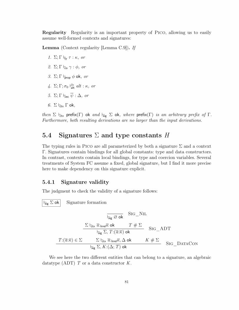
Regularity Regularity is an important property of Pico, allowing us to easilyassume well-formed contexts and signatures:

Lemma (Context regularity [Lemma C.9]). If

1. Σ; Γ ty τ : κ, or

2. Σ; Γ co γ : φ, or

3. Σ; Γ prop φ ok, or

4. Σ; Γ;σ0 `τ0alt alt : κ, or

5. Σ; Γ vec ψ : ∆, or

6. Σ ctx Γ ok,

then Σ ctx prefix(Γ) ok and sig Σ ok, where prefix(Γ) is an arbitrary prefix of Γ.Furthermore, both resulting derivations are no larger than the input derivations.

5.4 Signatures Σ and type constants H

The typing rules in Pico are all parameterized by both a signature Σ and a contextΓ. Signatures contain bindings for all global constants: type and data constructors.In contrast, contexts contain local bindings, for type and coercion variables. Severaltreatments of System FC assume a fixed, global signature, but I find it more precisehere to make dependency on this signature explicit.

5.4.1 Signature validity

The judgment to check the validity of a signature follows:

sig Σ ok Signature formation

sig ∅ okSig_Nil

Σ ctx a:Irrelκ ok T # Σ

sig Σ,T :(a:κ) okSig_ADT

T :(a:κ) ∈ Σ Σ ctx a:Irrelκ,∆ ok K # Σ

sig Σ,K :(∆;T ) okSig_DataCon

We see here the two different entities that can belong to a signature, an algebraicdatatype (ADT) T or a data constructor K .

81

An ADT is classified only by its list of universally quantified variables (oftenshortened to universals), as this is the only piece of information that varies betweenADTs. For example, the Haskell type Int contains no universals, while Either containstwo (both of kind Type), and Proxy ’s universals are (a : Type, b : a). The relevanceof universals is predetermined (see Section 5.4.2.2) and so no relevance annotationsappear on ADT specifications. Additionally, coercion variables are not permittedhere—coercion variables would be very much akin to Haskell’s misfeature of datatypecontexts49 and so are excluded.

A data constructor is classified by a telescope ∆ of existentially bound variables(or existentials) and the ADT to which it belongs. The grammar for telescopes is thesame as that for contexts, but we use the metavariables Γ and ∆ in distinct ways: Γis used as the context for typing judgments, whereas ∆ is more often used as somecomponent of a type. A telescope is a list of binders—both type variables and coercionvariables—where later binders may depend on earlier ones. A data constructor’sexistentials are the data that cannot be determined from an applied data constructor’stype. In this formulation, the term existential also includes what would normally beconsidered term-level arguments.

For example, let’s consider these Haskell definitions:

data Tuple a whereMkTuple :: ∀ a. Int → Char → a→ Tuple a

data Ex a whereMkEx :: ∀ a b. b → a→ Ex a

If I have a value of type Tuple Double, then I know the types of the data stored in aMkTuple, but I do not know the Int, the Char , or the Double—these are the existentials.Similarly, if I have a value of type Ex Char , then I know the type of one argument toMkEx , but I do not know the type of the other; I also know neither value. In this case,the second type, b, is existential, as are both values (of types b and a, respectively).

The use of the term existential to refer to term-level arguments may be non-standard, but it is quite convenient (while remaining technically accurate) in thecontext of a pure type system with ADTs.

5.4.2 Looking up type constants

Information about type constants is retrieved via the Σ tc H : ∆1; ∆2;H ′ judgment,presented in Figure 5.5 on the following page. This judgment retrieves three pieces ofdata about a type constant H : its universals, its existentials, and the head of the resulttype. It is best understood in concert with the typing rule that handles type constants,which also uses the typing judgment on vectors—ordered lists of arguments—alsopresented in Figure 5.5 on the next page. Let’s tackle this all in order of complexity.

49See discussion of how this is a misfeature at https://prime.haskell.org/wiki/NoDatatypeContexts.

82

Σ tc H : ∆1; ∆2;H ′ Σ ctx Γ okΣ; Rel(Γ) vec τ : Rel(∆1)

Σ; Γ ty Hτ : ’Π(∆2[τ/dom(∆1)]).H ′ τTy_Con

Σ tc H : ∆1; ∆2;H ′Type constant kinds, with universals ∆1,existentials ∆2, and result H ′

Σ tc Type : ∅;∅; TypeTc_Type

T :(a:κ) ∈ Σ

Σ tc T : ∅; a:Relκ; TypeTc_ADT

K :(∆;T ) ∈ Σ T :(a:κ) ∈ Σ

Σ tc K : a:Irrelκ; ∆;TTc_DataCon

Σ; Γ vec ψ : ∆ Type vector formation

Σ ctx Γ ok

Σ; Γ vec ∅ : ∅Vec_Nil

Σ; Γ ty τ : κ

Σ; Γ vec ψ : ∆[τ/a]

Σ; Γ vec τ, ψ : a:Relκ,∆Vec_TyRel

Σ; Rel(Γ) ty τ : κ

Σ; Γ vec ψ : ∆[τ/a]

Σ; Γ vec τ, ψ : a:Irrelκ,∆Vec_TyIrrel

Σ; Rel(Γ) co γ : φ

Σ; Γ vec ψ : ∆[γ/c]

Σ; Γ vec γ, ψ : c:φ,∆Vec_Co

Figure 5.5: Type constants H and vectors ψ

83

5.4.2.1 The constant Type

The constant Type has no universals, no existentials, and Type’s type is Type, asTc_Type tells us. Thus, in the use of Ty_Con when Hτ is just Type (normally,we omit such empty braces), we see that ∆1, ∆2, and τ are all empty, meaning thatwe get Σ; Γ ty Type : Type, as desired.

5.4.2.2 Algebraic datatypes

Let’s consider Maybe as an example. We see that the list of universals ∆1 is empty forall ADTs. Thus, the list of universal arguments τ must be empty in Ty_Con. The listof existentials ∆2 is a:RelType and the result type root is Type, both by Tc_ADT.We thus get Σ; Γ ty Maybe : ’Πa:RelType.Type, as desired. (Note that a is unused inthe body of the ’Π and thus that this type could also be written as Type→ Type.)

I have argued here how the rules work out this case correctly, but it may surprisethe reader to see that the argument to Maybe is treated as an existential here—partof ∆2—and not a universal. This could best be understood if we consider Type itselfto be an open ADT (that is, an extensible ADT) with no universal parameters. Tomake this even more concrete, here is how it might look in Haskell:

data Type whereBool :: TypeInt :: TypeMaybe :: Type→ TypeProxy :: ∀ (k :: Type). k → Type...

Thinking of ADTs this way, we can see why the argument to Maybe is existential,just like other arguments to constructors (see Section 5.4.1 for an explanation of theunusual use of the word existential here). We can also see that the kind parameter kto Proxy is also considered an existential in this context.

The last detail to cover here is the relevance annotation on the a, as assignedin Tc_ADT: all the variables are considered relevant. This is a free choice in thedesign of Pico. Any choice of relevance annotations would work, including allowingthe user to decide on a case-by-case basis. I have chosen to mark them as relevant,however, with the consideration that these ADTs might be present at runtime. Thereis nothing in Pico that restricts ADTs to be present only at compile time; the usermight write a runtime computation that returns Bool , for example.50 (Such a facilityreplaces Haskell’s current TypeRep facility [75].) By marking the ADT parameters asrelevant, a runtime decision can be made between, say, Maybe Int and Maybe Bool .This seems useful, and so I have decided to make these parameters relevant.

50This statement does not mean that you can extract the value Maybe Int from Just 3, whichwould require preserving all types for runtime.

84

5.4.2.3 Data constructors

The most involved case is that for data constructors, where both the universals andthe existentials can be non-empty. We’ll try to understand Ty_Con first by anexample inspired by the Haskell expression Left True :: Either Bool Char . Let’s recallthe definition of Either , a basic sum type:

data Either :: Type→ Type→ Type whereLeft :: a→ Either a bRight :: b → Either a b

In Pico this looks like the following:

Σ =Either :(a : Type, b : Type), Left:(x :Rela;Either),Right:(x :Relb;Either),Bool :(∅),True:(∅;Bool),False:(∅;Bool),Char :(∅)

Σ;∅ ty LeftBool ,Char True : Either Bool Char

We see how the universal arguments Bool and Char to the constructor Left are specifiedin the subscript; without these arguments, there would be no way to get the type ofLeft True in a syntax-directed way.

Universal argument saturation The grammar for type constant occurrences intypes requires them to appear fully saturated with respect to universals but perhapsunsaturated with respect to existentials. There are several reasons for this seeminglypeculiar design:

• It is helpful to separate universals from existentials in a variety of contexts. Forexample, existentials are brought into scope on a case-match, while universals arenot. Separating out these arguments is also essential in the step rule S_KPush.

• If Pico did not allow matching on unsaturated constants, it might be mostnatural to require saturation with respect to both universals and existentials(while still keeping these different arguments separate). This would allow, forexample, for a simple statement of the canonical forms lemma (Lemma C.75),because only a λ-expression would have a Π-type.

However, since Pico does allow matching on unsaturated constants, the grammarmust permit this form. Because Pico tracks the difference between matchable’Π and unmatchable

˜Π, we retain the simplicity of the canonical forms lemma,

as any expression classified by a ’Π must be a partially applied constant and anyexpression classified by a

˜Π must be a λ.

• All universal arguments are always irrelevant and erased during type erasure(Section 5.11). It is thus natural to separate these from existentials in thegrammar.

85

As with many design decisions, it is possible to redesign Pico and avoid thisunusual choice, but in my opinion, this design pays its weight nicely.

Typing rules for data constructors The Tc_DataCon rule looks up a dataconstructor K in the signature Σ to find its telescope of existentials ∆ and parentdatatype T . The second premise of the rule then looks up T to get the universals.The universals are annotated with Irrel, as universals are always irrelevant in dataconstructors—universal arguments are properly part of the type of a data constructorand are thus not needed at runtime. The telescope of existentials ∆ and datatype Tare also returned from tc.

Rule Ty_Con checks the supplied arguments τ against the telescope of universals,here named ∆1. Note that τ are checked against Rel(∆1); the braces that appear inthe production Hτ are part of the concrete syntax and do not represent wrappingeach individual τ ∈ τ in braces (cf. Section 5.6.2). Rule Ty_Con then builds theresult type, a ’Π-type binding the existentials and producing H ′—that is, the parenttype T—applied to all of the universals.

5.5 ExamplesThough these examples may make sense more fully after reading the sections below, itmay be helpful at this point to see a few short examples of Pico programs.

We will work with a definition of length-indexed vectors, a tried-and-true exampleof the design of GADTs. Here is how they are declared in Haskell (further explanationis available in Section 3.1.1):

data Nat = Zero | Succ Natdata Vec :: Type→ Nat → Type whereVNil :: Vec a 0VCons :: a→ Vec a n→ Vec a ( ’Succ n)

If Pico had a concrete syntax, these declarations would be transformed roughly intothe following:

Nat :: TypeZero :: NatSucc :: Nat → NatVec :: Type→ Nat → TypeVNil :: ∀ (a :: Type) (n :: Nat). (n ∼ Zero)→ Vec a nVCons :: ∀ (a :: Type) (n :: Nat).

∀ (m :: Nat). (n ∼ Succ m)→ a→ Vec a m→ Vec a n

The change seen here is just the transformation between specifying a GADT equalityconstraint via a return type in a declaration to using an explicit existential variablewith an explicit equality constraint.

86

In the abstract syntax of Pico, these declarations are represented by this signatureΣ0:

Σ0 =Nat:(∅),Zero:(∅;Nat),Succ :(_:RelNat;Nat),Vec :(a : Type, n : Nat),VNil :(c:n ∼ 0;Vec),VCons:(m:IrrelNat, c:n ∼ Succ m,_:Rela,_:RelVec am;Vec)

Let’s walk through these declarations. Our binding for Nat includes an empty list ofuniversally quantified type variables. This binding is followed by specifications forZero, which lists no existential variables and is a constructor of the datatype Nat, andSucc , which has one (anonymous) existential variable and also belongs to Nat. Thebindings for Vec and its constructors are similar, but with more parameters. Note thecoercion bindings in the telescopes associated with VNil and VCons, as well as theirrelevant binding for the existential m of VCons. The design we see here, echoing theHaskell, does not permit runtime extraction of the length of a vector. If we changedthe m to be relevant, then runtime length extraction would be trivial.

We will now look at a few simple operations on vectors, first in Haskell and thenin Pico.51

5.5.1 isEmpty

First, a very simple test for emptiness, in order to familiarize ourselves with pattern-match syntax in Pico:

isEmpty :: Vec a n→ BoolisEmpty VNil = TrueisEmpty (VCons ) = False

Translated to Pico, we get the following:

isEmpty :˜Π(a:IrrelType), (n:IrrelNat), (v :RelVec a n).Bool

isEmpty =λ(a:IrrelType), (n:IrrelNat), (v :RelVec a n).caseBool v of

VNil → λ(c:n ∼ 0), (c0:v ∼ VNila,n c).TrueVCons→ λ(m:IrrelNat), (c:n ∼ Succ m), (x :Rela), (xs:RelVec am),

(c0:v ∼ VConsa,nm c x xs).False

The most striking feature about this Pico code is the form of the case expression.Unlike the concrete syntax of Haskell, patterns in Pico do not directly bind any

51In these examples, I assume the use of numerals to specify elements of type Nat, and I alsoassume the existence of, e.g., Bool .

87

arguments. Note that there are no variable bindings to the left of the arrows in thecase-branches. Instead, I have chosen to have λs to the right of the arrow. This designchoice greatly simplifies the typing and scoping rules for pattern matches, because itremoves a binding site in the grammar (leaving us with two: Π and λ). Because of thetyping rule for case expressions (Section 5.6.5), we still must bind all of the existentialsof a data constructor when matching against it—even when these existentials areignored, as we see here.

The matches also bind a variable not mentioned in the data constructors’ exis-tentials: the coercion variable c0. This coercion witnesses the equality between thescrutinee (v , in this case) and the applied data constructor that introduces the casebranch. This coercion variable is bound in all matches, meaning that all patternmatching in Pico is dependent pattern matching.52

The behavior of case can also be viewed through its operational semantics, ascaptured in the following rule, excerpted from Section 5.7.2:

alti = H → τ0

Σ; Γ s caseκHτ ψ of alt −→ τ0 ψ 〈Hτ ψ〉S_Match

Note that the body of the match, τ0, is applied to the existential arguments to Hτand a coercion witnessing the equality between the scrutinee and the pattern. In thecase of a successful match, this coercion is reflexive, as denoted by the angle brackets〈Hτ ψ〉.

5.5.2 replicate

Let’s now look at replicate, one of the simplest functions that requires a proper Π-type.First, in Haskell:

replicate :: Π n→ a→ Vec a nreplicate Zero = VNilreplicate (Succ m) x = VCons x (replicate m x)

52Contrast to Gundry [37], who use two separate constructs, case and dcase, only the latterof which does dependent matching. This separation is necessary in his language because not allexpressions can be used in types and thus in dependent pattern matching. In particular, Gundryprevents λ-expressions in types, a limitation I have avoided by maintaining the distinction betweenmatchable and unmatchable Π-types.

88

Now, in Pico:

replicate :˜Π(a:IrrelType), (n:RelNat), (x :Rela).Vec a n

replicate =λa:IrrelType.fixλ(r :Rel

˜Π(n:RelNat), (x :Rela).Vec a n),

(n:RelNat), (x :Rela).caseVec a n n of

Zero → λc0:(n ∼ Zero).VNila,n c0

Succ→ λm:RelNat, c0:(n ∼ Succ m).VConsa,n m c0 x (r m x)

This example shows the (standard) use of fix as well as some of the more exoticfeatures of Pico. In the case branches, we see how we pass universal arguments tothe data constructors VNil and VCons. We also see how we have to wrap irrelevantarguments (the m in the last line) in braces. This example also shows where thecoercion variable c0 comes into play: it’s needed to provide the coercion to the VNiland VCons constructors to prove that the universal argument n is indeed of the shaperequired for these constructors. Without the ability to do a dependent pattern match,this example would be impossible to write, unless you fake dependent types usingsingletons or some other technique.

5.5.3 append

We’ll now examine how to append two vectors. This operation will also require theuse of an addition operation, defined using prefix notation so as not to pose a parsingchallenge:

plus :: Nat → Nat → Natplus Zero n = nplus (Succ m) n = Succ (plus m n)

append :: Vec a m→ Vec a n→ Vec a ( ’plus m n)append VNil ys = ysappend (VCons x xs) ys = VCons x (append xs ys)

89

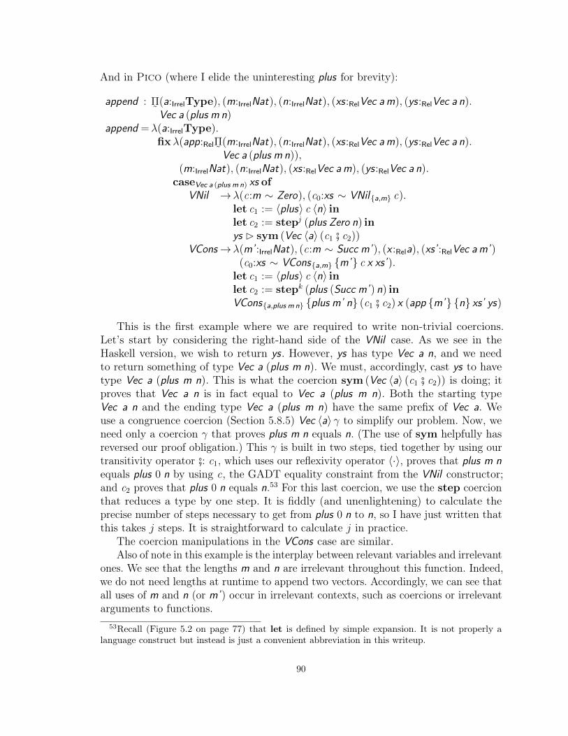
And in Pico (where I elide the uninteresting plus for brevity):

append :˜Π(a:IrrelType), (m:IrrelNat), (n:IrrelNat), (xs:RelVec am), (ys:RelVec a n).Vec a (plus m n)

append =λ(a:IrrelType).fixλ(app:Rel

˜Π(m:IrrelNat), (n:IrrelNat), (xs:RelVec am), (ys:RelVec a n).Vec a (plus m n)),

(m:IrrelNat), (n:IrrelNat), (xs:RelVec am), (ys:RelVec a n).caseVec a (plus m n) xs of

VNil →λ(c:m ∼ Zero), (c0:xs ∼ VNila,m c).let c1 := 〈plus〉 c 〈n〉 inlet c2 := stepj (plus Zero n) inys B sym (Vec 〈a〉 (c1 # c2))

VCons→λ(m’ :IrrelNat), (c:m ∼ Succ m’), (x :Rela), (xs’ :RelVec am’)(c0:xs ∼ VConsa,m m’ c x xs’).

let c1 := 〈plus〉 c 〈n〉 inlet c2 := stepk (plus (Succ m’) n) inVConsa,plus m n plus m’ n (c1 # c2) x (app m’ n xs’ ys)

This is the first example where we are required to write non-trivial coercions.Let’s start by considering the right-hand side of the VNil case. As we see in theHaskell version, we wish to return ys. However, ys has type Vec a n, and we needto return something of type Vec a (plus m n). We must, accordingly, cast ys to havetype Vec a (plus m n). This is what the coercion sym (Vec 〈a〉 (c1 # c2)) is doing; itproves that Vec a n is in fact equal to Vec a (plus m n). Both the starting typeVec a n and the ending type Vec a (plus m n) have the same prefix of Vec a. Weuse a congruence coercion (Section 5.8.5) Vec 〈a〉 γ to simplify our problem. Now, weneed only a coercion γ that proves plus m n equals n. (The use of sym helpfully hasreversed our proof obligation.) This γ is built in two steps, tied together by using ourtransitivity operator #: c1, which uses our reflexivity operator 〈·〉, proves that plus m nequals plus 0 n by using c, the GADT equality constraint from the VNil constructor;and c2 proves that plus 0 n equals n.53 For this last coercion, we use the step coercionthat reduces a type by one step. It is fiddly (and unenlightening) to calculate theprecise number of steps necessary to get from plus 0 n to n, so I have just written thatthis takes j steps. It is straightforward to calculate j in practice.

The coercion manipulations in the VCons case are similar.Also of note in this example is the interplay between relevant variables and irrelevant

ones. We see that the lengths m and n are irrelevant throughout this function. Indeed,we do not need lengths at runtime to append two vectors. Accordingly, we can see thatall uses of m and n (or m’) occur in irrelevant contexts, such as coercions or irrelevantarguments to functions.

53Recall (Figure 5.2 on page 77) that let is defined by simple expansion. It is not properly alanguage construct but instead is just a convenient abbreviation in this writeup.

90

5.5.4 safeHead

With length-indexed vectors, we can write a safe head operation, allowed only whenwe know that the vector has a non-zero length:

safeHead :: Vec a ( ’Succ n)→ asafeHead (VCons x ) = x

Note that safeHead contains a total pattern match; the VNil alternative is impossiblegiven the type signature of the function. This function translates to Pico thusly:

safeHead :˜Π(a:IrrelType), (n:IrrelNat), (v :RelVec a (Succ n)). a

safeHead =λ(a:IrrelType), (n:IrrelNat), (v :RelVec a (Succ n)).casea v ofVNil → λ(c:Succ n ∼ Zero), (c0:v ∼ VNila,Succ n c). absurd c aVCons→ λ(m:IrrelNat), (c:Succ n ∼ Succ m), (x :Rela), (xs:RelVec am),

(c0:v ∼ VConsa,Succ n m c x xs).x

The new feature demonstrated in this example is the absurd operator, whichappears in the body of the VNil case. In order to be sure that case expressions donot get stuck, the typing rules require that all matches are exhaustive. However, ingeneral, in can be undecidable to determine whether the type of a scrutinee indicatesthat a certain constructor can be excluded. In order to step around this potentialtrap, Pico supports absurdity elimination through absurd. The coercion passed intoabsurd (c, above) must prove that one constant equals another. This is, of course,impossible, and so we allow absurd γ τ to have any type τ .

5.6 Types τHaving gone through several examples explaining the flavor of Pico code, let’s nowwalk through the remaining typing rules of the system. Recall that we have alreadyseen the typing rules for variables, Ty_Var in Section 5.3, and constants, Ty_Conin Section 5.4.2.

91

5.6.1 Abstractions

The definition for types τ includes the usual productions for a pure type system,including both a Π-form and a λ-form:

Σ; Γ,Rel(δ) ty κ : Type

Σ; Γ ty Πδ. κ : TypeTy_Pi

Σ; Γ, δ ty τ : κ

Σ; Γ ty λδ. τ :˜Πδ. κ

Ty_Lam

The only novel component of these rules is the use of Rel(δ) in the premise to Ty_Pi.This is done to allow the bound variable to appear in κ, regardless of whether it isrelevant or not. As an example, the use of Rel(δ) here is necessary to allow the type ofHaskell’s ⊥:

˜Πa:IrrelType. a.

5.6.2 Applications

Terms with a Π-type (either type constants or λ-terms) can be applied to arguments,via these rules:

Σ; Γ ty τ1 : Πa:Relκ1. κ2 Σ; Γ ty τ2 : κ1

Σ; Γ ty τ1 τ2 : κ2[τ2/a]Ty_AppRel

Σ; Γ ty τ1 : Πa:Irrelκ1. κ2 Σ; Rel(Γ) ty τ2 : κ1

Σ; Γ ty τ1 τ2 : κ2[τ2/a]Ty_AppIrrel

Σ; Γ ty τ : Πc:φ. κ Σ; Rel(Γ) co γ : φ

Σ; Γ ty τ γ : κ[γ/c]Ty_CApp

We see in these rules that the argument form for an abstraction over an irrelevantbinder requires braces. (See the conclusion of Ty_AppIrrel.) The system wouldremain syntax-directed without marking off irrelevant arguments, but type erasure(Section 5.11) would then need to be type-directed. It seems easier just to separaterelevant arguments from irrelevant arguments syntactically.

Note also the use of Rel(Γ) in Ty_AppIrrel and Ty_CApp; resetting thecontext here happens because irrelevant arguments and coercions are erased in therunning program.

92

5.6.3 Kind casts

We can always use an equality to change the kind of a type:

Σ; Rel(Γ) co γ : κ1 ∼ κ2

Σ; Γ ty τ : κ1 Σ; Rel(Γ) ty κ2 : Type

Σ; Γ ty τ B γ : κ2

Ty_Cast

In this rule, a type of kind κ1 is cast by γ to have a type κ2. As always, the coercionis checked in a reset context Rel(Γ). The final premise, Σ; Rel(Γ) ty κ2 : Type isimplied by the first premise (which is actually Σ; Rel(Γ) co γ : κ1

Type∼Type κ2) viaproposition regularity, but we must include it in order to prove kind regularity54 beforewe prove coercion regularity.

5.6.4 fix

Pico supports fixpoints via the following rule:

Σ; Γ ty τ :˜Πa:Relκ. κ

Σ; Γ ty fix τ : κTy_Fix

The rule requires type τ to have an unmatchable˜Π so that we can be sure that τ ’s

canonical form is indeed a λ (as opposed to an unsaturated constant); otherwise theprogress theorem (Section 5.7) would not hold.

5.6.5 case

Unsurprisingly, the typing rules to support pattern matching are the most involvedand are presented in Figure 5.6 on the following page with the rules to type-checkcase branches.

Most of the premises of Ty_Case are easy enough to explain:

• The result kind of a case, κ is given right in the syntax; the first premiseΣ; Rel(Γ) ty κ : Type ensures that it is a valid result kind.

• We also must check the kind of the scrutinee, τ . This kind must have theform ’Π∆.H σ (note the matchable ’Π), where the σ cannot mention any of thevariables bound in ∆. (The Σ; Rel(Γ) ty H σ : Type premise checks this scopingcondition.) Note that the scrutinee’s type may be a ’Π-type in order to supportmatching against partially applied type and data constructors.

• The alternatives must be exhaustive and distinct. Exhaustivity is needed toprove that a well-typed case cannot get stuck, and distinctness is necessary toprove that the reduction relation is deterministic.

54Both regularity lemmas are stated in Figure 5.3 on page 78.

93

Σ; Rel(Γ) ty κ : Type Σ; Γ ty τ : σσ = ’Π∆.H σ Σ; Rel(Γ) ty H σ : Type∀i , Σ; Γ;σ `τalt alti : κ

alt are exhaustive and distinct for H , (w.r.t. Σ)Σ; Γ ty caseκ τ of alt : κ

Ty_Case

Σ; Γ;σ `τalt alt : κ Case alternatives

Σ tc H : ∆1; ∆2;H ′ ∆3,∆4 = ∆2[σ/dom(∆1)]dom(∆4) = dom(∆′)matchdom(∆3)(types(∆4); types(∆′)) = Just θΣ; Γ ty τ : ?Π∆3, c:τ0 ∼ Hσ dom(∆3). κ

Σ; Γ; ’Π∆′.H ′ σ `τ0alt H → τ : κAlt_Match

Σ; Γ ty τ : κ

Σ; Γ;σ `τ0alt _→ τ : κAlt_Default

types(∆) = τ Extract the types from a telescope

types(∅) = ∅types(∆, a:ρκ) = types(∆), κ

types(∆, c:τ1κ1∼κ2 τ2) = types(∆), κ1, κ2, τ1, τ2

Figure 5.6: Rule and auxiliary definitions for case expressions

We are left to consider type-checking the alternatives. This is done via the judgmentwith schema Σ; Γ; σ `τalt alt : κ. When Σ; Γ; σ `τalt alt : κ holds, we know that theexpression in the case alternative alt produces a type of kind κ when considered withsignature Σ and typing context Γ and when matched against a scrutinee τ of type σ.The premises of Ty_Case indeed check that all alternatives satisfy this judgment.

5.6.5.1 Checking case alternatives

The rule Alt_Match is intricate. It assumes a scrutinee τ0 of type ’Π∆′.H ′ σ, andwe are checking a case alternative H → τ .

First, we must verify that the constant H is classified by H ′—that is, either H isa data constructor of the datatype H ′ or H is a datatype and H ′ is Type. We saythat H ′ is the parent of H . This check is done by the Σ tc H : ∆1; ∆2;H

′ premise,which also extracts the universals ∆1 and existentials ∆2.

The next premise (reading to the right) uses ∆2[σ/dom(∆1)] to instantiate theexistentials with the known choices for the universals. These known choices σ areobtained from determining the type of the scrutinee; see the appearance of σ in the

94

type appearing before the alt in the conclusion of the rule. The second premise alsosplits the instantiated existentials into two telescopes, ∆3 and ∆4.

Note that ∆′ is an input to this rule; it is extracted from the type of the scrutinee.Accordingly, the third premise dom(∆4) = dom(∆′) serves two roles: it fixes the lengthof ∆4 (and, hence, ∆3) and it also forces any renaming of bound variables necessaryto line up the telescopes ∆′ and ∆4. Keeping the names of the bound variablesconsistent between these telescopes simplifies this rule. We see that in the event thatthe scrutinee is a fully saturated datatype or data constructor, ∆4 = ∆′ = ∅ and∆3 = ∆2[σ/dom(∆1)]; in this common case, then, unification is unnecessary.

The next premise uses a one-way unification algorithm to make sure that thebound telescope in the scrutinee’s type, ∆′, matches the expected shape ∆4. (Thetypes operation appears in Figure 5.6 on the previous page.) We will return to this inSection 5.6.5.2, below. In the common case of ∆′ = ∅ (that is, full saturation of thescrutinee), this premise is trivially satisfied. Also note that we do not use the outputof this premise, θ, anywhere in the rule, so skipping it on a first reading is appropriate.

Lastly, we must check that the body of the alternative, τ , has the right type. Thistype must bind (by any combination of matchable ’Π and unmatchable

˜Π—recall

that this is the meaning of ?Π from Figure 5.2 on page 77) all of the existentials in∆3, as well as the coercion variable witnessing the equality between τ0 (the scrutinee)and the applied H . In this rule the use of dom(∆3) as a list of arguments to Hσ isa small pun; we must imagine braces surrounding any variable in dom(∆3) that isirrelevantly bound. The return type of the abstraction in τ must be κ, the result kindof the overall match.

For examples of this in action—at least in the fully saturated case—see the workedout examples above (Section 5.5).

5.6.5.2 Unification in Alt_Match

Let’s examine the use of unification in Alt_Match more carefully. We will proceedby examining two examples, a simple one where unification is unnecessary and a moreinvolved one showing why we sometimes need it.

Our first example was given above, when first describing unsaturated matching(Section 5.1.1.2):

type family IsLeft x whereIsLeft ’Left = ’TrueIsLeft ’Right = ’False

The translation of Either into Pico appears in Section 5.4.2.3. This type familytranslated to the following Pico function (rewritten to be lowercase according to

95

Haskell naming requirements):

isLeft :˜Π(a:IrrelType), (x :Rel’Π(y :Rela).Either a a).Bool

isLeft =λ(a:IrrelType), (x :Rel’Π(y :Rela).Either a a).caseBool x of

Left → λc0:(x ∼ Lefta,a).TrueRight→ λc0:(x ∼ Righta,a).False

Comparing the first alternative against Alt_Match, we see the following concreteinstantiations of metavariables:

H = Left∆1 = s:IrrelType, t:IrrelType∆2 = y :RelsH ′= Eitherτ0 = x∆′= y :Rela

σ= a, a∆3 = ∅∆4 = y :Relaθ= ∅τ = λ(c0:x ∼ Lefta,a).Trueκ= Bool

In this example, the constructor is not applied to any existential variables, and so∆3, the telescope of binders that are to be bound by the match, is empty. The onlyvariable bound in the match body is c0, the dependent-match coercion variable. Alsonote that ∆4, the instantiated suffix of the telescope of existential arguments to Left,and ∆′, the telescope of binders in the type of the scrutinee, coincide. Accordingly,the match operation succeeds with an empty substitution θ = ∅.

In contrast, the following example shows why we need unification in Alt_Match:

data X whereMkX :: a→ a→ X

-- NB: a is existential; no universals heretype family UnX (x :: Bool ’→X ) :: Bool whereUnX ( ’MkX y) = y

Note that we’re extracting the first (visible) argument from an unsaturated use ofMkX . This Haskell code translates to the following Pico:

Σ =X :(∅),MkX :(a:IrrelType, y :Rela, z :Rela;X )

unX :˜Π(x :Rel’Π(z :RelBool).X ).Bool

unX =λ(x :Rel’Π(z :RelBool).X ).caseBool x ofMkX → λ(a:IrrelType), (y :Rela), (c0:x ’Π(z:RelBool).X∼’Π(z:Rela).X MkX a y).

y B sym (argk (kind c0))

Before we get into the minutiae of Alt_Match, let’s dwell a moment on the cast

96

necessary in the last line. According to both the type of unX and the return typeprovided in the case, the match must return something of type Bool . Yet the body ofa match must bind precisely the existential variables of a data constructor; accordingto the definition of MkX , the variable y has type a, not Bool . We thus must cast yfrom a to Bool . We do this by extracting out the right coercion from c0. This c0 isheterogeneous; I have typeset the code above with the kinds explicit to show this.The left-hand kind is the declared type of x , binding z of type Bool . The right-handkind is the kind of MkX a y , which binds z of type a. By using kind (which extractsa kind equality from a heterogeneous coercion; see Section 5.8.1), followed by argk(which extracts a coercion between the kinds of the arguments of Π-types; see Section5.8.6.1), and then sym (which reverses the orientation of a coercion), we get thecoercion needed, of type a ∼ Bool .

Now, we’ll try to understand the matching in Alt_Match. Let’s once againexamine the concrete instantiations of the metavariables in the rule:

H = MkX∆1 = ∅∆2 = a:IrrelType, y :Rela, z :RelaH ′= Xτ0 = x∆′= z :RelBool

σ= ∅∆3 = a:IrrelType, y :Rela∆4 = z :Relaθ= Bool/aτ = 〈as above〉κ= Bool

Recall that ∆3 and ∆4 are the prefix and suffix, respectively, of the telescope ofexistentials ∆2, after this telescope has been instantiated with the known argumentsfor the universals. However, with MkX , there are no universals at all (the datatypeX takes no arguments), and so this instantiation is a no-op. (The lack of universalsshows up in the equations above via an empty ∆1 and an empty σ.) We thus have∆3,∆4 = ∆2, where the length of ∆4 must match the length of ∆′, the telescopeof variables bound in the type of the scrutinee. We see that the scrutinee x hastype ’Π(z :RelBool).X and so ∆′ = z :RelBool . Thus ∆3—the existentials bound by thepattern match—has two elements (a and y) and ∆4 has one (z).

We now must make sure that the shape of the types in ∆′ match the templategiven by the types in ∆4. That is, ∆′ must be some instance of ∆4, as determinedby a unification algorithm (discussed in more depth in Section 7.3). In this case, theunification succeeds, assigning the type variable a to be Bool , as shown in the choicefor θ, above. Accordingly, the match is well typed.

Requiring this unification simply reduces the set of well typed programs. It is thusimportant to understand why the restriction is necessary. What goes wrong if we omitit? The problem comes up in the proof for progress, in the case where the scrutineehas a top-level cast. We will use step rule S_KPush (see Section 5.9); that rule hasseveral typing premises55 which can be satisfied only when this match succeeds. Therestriction is quite technical in nature, but any alternative not ruled out by the type

55These unexpected typing premises to a small-step reduction rule are addressed in Section 5.7.4.

97

of the scrutinee should be acceptable. See the proof of progress in Appendix C.11 forthe precise details.

5.6.5.3 Default alternatives

Pico supports default alternatives through the form _ → τ . This is a catch-allcase, to be used only when no other case matches. In a language with a simplertreatment for case statements, a default would be unnecessary; every case couldsimply enumerate all possible constructors. However, Pico has two features thatmakes defaults indispensable:

• When matching on a scrutinee of kind Type (or, say, a function returning aType), it would be impossible to enumerate all possibilities of this open type.Such matches must have a default alternative.

• If a scrutinee is partially applied, the typing rules dictate a delicate unificationprocess to make sure alternatives are well typed. (See Section 5.6.5.2.) Giventhe design of Alt_Match, it is possible some of the constructors of a datatypewould be ill typed as patterns in an unsaturated match. It might therefore bechallenging to detect whether an unsaturated match is exhaustive. To avoidthis problem, unsaturated matches may use a default alternative in order to beunimpeachably exhaustive.

Happily, the typing rule Alt_Default for default alternatives could hardly besimpler.

5.6.5.4 Absurdity

We saw in the safeHead example (Section 5.5.4) the need for absurdity eliminationvia the absurd operator. Here is the typing rule:

Σ; Rel(Γ) co γ : H1τ1 ψ1 ∼ H2τ2 ψ2 H1 6= H2

Σ; Rel(Γ) ty τ : Type

Σ; Γ ty absurd γ τ : τTy_Absurd

This rule requires that the coercion argument to absurd, γ, relate two unequal typeconstants H1 and H2. The type absurd γ τ can have any well formed kind, as chosenby τ . Because τ is needed only to choose the overall kind of the type, it is checked acontext reset by Rel.

As explained with the example, absurdity elimination is sometimes needed inthe body of case alternatives that can never be reached. In a language that admitsundefined , the absurd construct is not strictly necessary. Yet by including it, we candefinitively mark those alternatives that are unreachable. Simply returning undefinedwould not be as informative.

98

5.7 Operational semanticsNow that we have seen the static semantics of types, we are well placed to exploretheir dynamic semantics—how the types can reduce to values. The dynamic semanticsof types is expressed in Pico via a small-step operational semantics, captured in thejudgment Σ; Γ s τ −→ τ ′. Rules in this judgment are prefixed by “S_”. It must beparameterized over a typing environment because of the push rules, as explained inSection 5.7.4.

The operational semantics obeys preservation and progress theorems.

Theorem (Preservation [Theorem C.46]). If Σ; Γ ty τ : κ and Σ; Γ s τ −→ τ ′, thenΣ; Γ ty τ

′ : κ.

Theorem (Progress [Theorem C.78]). Assume Γ has only irrelevant variable bindings.If Σ; Γ ty τ : κ, then either τ is a value v , τ is a coerced value v B γ, or there exists τ ′such that Σ; Γ s τ −→ τ ′.

The progress theorem is non-standard in two different ways:

• As discussed shortly (Section 5.7.1), reduction can take place in a context withirrelevant variable bindings.

• The progress theorem guarantees that a stuck type is either a value v or acoerced value v B γ. This statement of the theorem follows previous work (suchas Weirich et al. [105]) and is applicable in the right spot in the proof of typeerasure (Section 5.11).

The operational semantics are also deterministic.

Lemma (Determinacy [Lemma C.20]). If Σ; Γ s τ −→ σ1 and Σ; Γ s τ −→ σ2, thenσ1 = σ2.

5.7.1 Values

A subset of the types τ are considered values, written with the metavariable v :

Definition (Values). Let values v be defined by the following sub-grammar of τ :

v ::=Hτ ψ |Πδ. τ |λa:Relκ. τ |λa:Irrelκ. v |λc:φ. τ

As we can see, values include applied constants, Π-types, and some λ-types.However, note a subtle but important part of this definition: the production forirrelevant abstractions is recursive. An irrelevant abstraction λa:Irrelκ. τ is a value ifand only if τ , the body, is also a value. This choice is important in order to prove typeerasure.

Our definition of values also gives us this convenient property:

99

Lemma (Value types [Lemma C.76]). If Σ; Γ ty v : κ, then κ is a value.

During compilation, we erase irrelevant components of an expression completely.This includes irrelevant abstractions. Thus, the erasure operation, written T·U andfurther explored in Section 5.11, includes this equation,

Tλa:Irrelκ. τU = TτU,

erasing the abstraction entirely. Yet we must make sure to maintain the followinglemma, referring to the definition of values on erased expressions:

Lemma (Expression redexes [Lemma C.84]). If TτU is not a value, then τ is not avalue.

If we have the equation above erasing irrelevant abstractions to the erasure of theirbodies but call all irrelevant abstractions values (that is, make λa:Irrelκ. τ a value for allτ), then this lemma becomes false. To wit, suppose τ is not a value. Then Tλa:Irrelκ. τUwould not be a value, but λa:Irrelκ. τ would be. Thus, in order to maintain this lemma,we have a recursive definition of values for irrelevant abstractions and, accordingly,evaluate under irrelevant abstractions as well. See rule S_IrrelAbs_Cong in Section5.7.3.

5.7.2 Reduction

Several of the small-step rules perform actual reduction in a type:

Σ; Γ s (λa:Relκ. σ1)˜σ2 −→ σ1[σ2/a]S_BetaRel

Σ; Γ s (λa:Irrelκ. v1)˜σ2 −→ v1[σ2/a]S_BetaIrrel

Σ; Γ s (λc:φ. σ)˜γ −→ σ[γ/c]S_CBeta

alti = H → τ0

Σ; Γ s caseκHτ ψ of alt −→ τ0 ψ 〈Hτ ψ〉S_Match

alti = _→ σ no alternative in alt matches HΣ; Γ s caseκHτ ψ of alt −→ σ

S_Default

alti = _→ σ no alternative in alt matches HΣ; Γ s caseκHτ ψ B γ of alt −→ σ

S_DefaultCo

τ = λa:Relκ. σ

Σ; Γ s fix τ −→ σ[fix τ/a]S_Unroll

100

Note that S_BetaIrrel requires a value v1 in the body of the abstraction in orderto keep the rules deterministic. The only other surprising feature in these rules is theway that S_Match works by applying the body of the alternative τ0 to the actualexistential arguments to Hτ and a reflexive coercion. This follows directly from mydesign of having case alternatives avoid a special binding form and use the existingforms in the language.

The Beta rules above make explicit that the application is an unmatchableapplication τ˜ψ. This is actually redundant, as all λ-abstractions are unmatchable. Ihave included the notation here to make it clearer how these rules line up with therules in the parallel rewrite relation used to prove consistency (Section 5.10.2).

5.7.3 Congruence forms

Pico has several uninteresting congruence forms,

Σ; Γ s σ −→ σ′

Σ; Γ s σ ψ −→ σ′ ψS_App_Cong

Σ; Γ s σ −→ σ′

Σ; Γ s σ B γ −→ σ′ B γS_Cast_Cong

Σ; Γ s σ −→ σ′

Σ; Γ s caseτ σ of alt −→ caseτ σ′ of altS_Case_Cong

Σ; Γ s τ −→ τ ′

Σ; Γ s fix τ −→ fix τ ′S_Fix_Cong

and one more unusual one:

Σ; Γ, a:Irrelκ s σ −→ σ′

Σ; Γ s λa:Irrelκ. σ −→ λa:Irrelκ. σ′S_IrrelAbs_Cong

This last rule allows for evaluation under irrelevant abstractions, as described inSection 5.7.1. It must add the new irrelevant variable to the context, but is otherwiseunexceptional.

5.7.4 Push rules

A system with explicit coercions like Pico must deal with the possibility that coercionsget in the way of reduction. For example, what happens when we try to reduce

((λx :RelBool . x)B 〈Bool〉)True ?

Casting by a reflexive coercion should hardly matter, and yet no rule yet describedapplies here. In particular, S_BetaRel does not.

101

Σ; Γ s (v B γ1)B γ2 −→ v B (γ1 # γ2)S_Trans

Σ; Rel(Γ) co γ0 : Πa:Relκ. σ ∼ Πa:Relκ′. σ′

γ1 = sym (argk γ0) γ2 = γ0@(τ B γ1 ≈sym γ1 τ)

Σ; Γ s (v B γ0) τ −→ v (τ B γ1)B γ2

S_PushRel

Σ; Rel(Γ) co γ0 : Πa:Irrelκ. σ ∼ Πa:Irrelκ′. σ′

γ1 = sym (argk γ0) γ2 = γ0@(τ B γ1 ≈sym γ1 τ)

Σ; Γ s (v B γ0) τ −→ v τ B γ1B γ2

S_PushIrrel

Σ; Rel(Γ) co γ0 : Πc:φ. σ ∼ Πc:φ′. σ′

γ1 = argk1 γ0 γ2 = argk2 γ0

η′ = γ1 # η # sym γ2 γ3 = γ0@(η′, η)

Σ; Γ s (v B γ0) η −→ v η′ B γ3

S_CPush

γ1 =˜Πa:Irrel〈κ〉. γ γ2 = τ1 ≈〈Type〉 τ2

τ1 =˜Πa:Irrelκ. (κ1[a B sym 〈κ〉/a]) τ2 =

˜Πa:Irrelκ. κ1

Σ; Γ s λa:Irrelκ. (v B γ) −→ (λa:Irrelκ. v)B (γ1 # γ2)S_APush

γ1 = γ0@(a ≈γ2 a B γ2) # sym γ2

γ2 = argk γ0

Σ; Γ s fix ((λa:Relκ. σ)B γ0) −→ (fix (λa:Relκ. (σ B γ1)))B γ2

S_FPush

Σ tc H : a:Irrelκ; ∆;H ′ ∆ = ∆1,∆2 n = |∆2|κ = ’Πa:Irrelκ,∆.H

′ a

σ = ’Π(∆2[τ/a][ψ/dom(∆1)]).H ′ τ

σ′ = ’Π(∆2[τ ′/a][ψ′/dom(∆1)]).H ′ τ ′

Σ; Rel(Γ) co η : σ ∼ σ′

Σ; Rel(Γ) vec τ′ : a:Relκ

∀i , γi = build_kpush_co(〈κ〉@(nths (resn η));ψ1...i−1)∀i , ψ′i = cast_kpush_arg(ψi ; γi)

H → κ′ ∈ alt

Σ; Γ s caseκ0 (Hτ ψ)B η of alt −→ caseκ0 Hτ ′ ψ′of alt

S_KPush

Figure 5.7: Push rules

102

To deal with this and similar scenarios, Pico follows the System FC tradition andcontains so-called push rules, as shown in Figure 5.7 on the previous page. These rulesare fiddly but—ignoring S_KPush for a moment—straightforward. They simply serveto rephrase a type with a coercion in the “wrong” place to an equivalent type with thecoercion moved out of the way. The rules can be derived simply by following the typingrules and a desire to push the coercion aside. Compared to previous work, the noveltyhere is in rules S_APush (which handles reduction under irrelevant abstractions andmust take into account the awkward substitution in Co_PiTy; see Section 5.8.5.1)and S_FPush (which handles fix, never before seen in System FC), but these rulesagain pose no design challenge other than the need for attention to detail.

Many of the push rules share an odd feature: they have typing judgment premises.These premises are the reason that the stepping judgment is parameterized on a typingcontext. In order to prove the progress theorem, it is necessary to prove consistency(Section 5.10), which basically says that no coercion (made without assumptions) canprove, say, Int ∼ Bool . Still ignoring S_KPush, the consistency lemma is enoughto admit the typing premises to the push rules. However, using consistency herewould mean that the preservation theorem depends on the consistency lemma, whileconsistency is normally used only to prove progress. In seems to lead to cleaner proofsto avoid the dependency of preservation on consistency, and so these typing premisesare necessary.

The S_KPush rule is very intricate and makes use of a variety of coercions.Explicating this rule in its entirety is best saved until after we have covered coercionsin more depth. See Section 5.9.

5.8 Coercions γPico comes with a very rich theory of equality, embodied in the large number ofcoercion forms. We will examine these forms in terms of the properties they imbueon the equality relation. Note that the coercion language is far from orthogonal; it isoften possible to prove one thing in multiple ways. Indeed, GHC comes with a coercionoptimizer [96] that transforms a coercion proving a certain proposition into another,simpler one proving the same proposition. Enhancing this optimizer is beyond thescope of this dissertation, however. It is needed only as an optimization in the speedof compilation and is not central to the theory or metatheory of the language.

All coercions are erased before runtime (Section 5.11). Accordingly, we check forwell typed coercions (via the judgment Σ; Γ co γ : φ) only in contexts reset by theRel(·) operator.

5.8.1 Equality is heterogeneous

The equality relation in Pico is heterogeneous, allowing ∼ to relate two types ofdifferent kinds. This is most clearly demonstrated in the rule for the well-formedness

103

of propositions:56

Σ; Γ prop φ ok Proposition formation

Σ; Γ ty τ1 : κ1

Σ; Γ ty τ2 : κ2

Σ; Γ prop τ1κ1∼κ2 τ2 ok

Prop_Equality

Note that the kinds κ1 and κ2 are allowed to differ.The particular flavor of heterogeneous equality in Pico is so-called “John Major”

equality [58], where an equality between two types implies the equality between thekinds:

Σ; Γ co γ : τ1κ1∼κ2 τ2

Σ; Γ co kind γ : κ1 ∼ κ2

Co_Kind

As we can see, the kind coercion form extracts a kind coercion from a type coercion.Though I have described my equality relation following McBride [58], he uses

identity proofs in quite a different way than I do here. His language confirms that anidentity proof is reflexive and then brings definitional equalities of the types and kindsinto scope. The surface Haskell version of heterogeneous equality works quite likeMcBride’s. My invocation of “John Major” here is to recall that an equality betweentypes implies the same relationship among the kinds.

It’s worth pausing here for a moment to consider two other possible meanings,among others, of heterogeneous equality:

Trellys equality The equality relation studied in the Trellys project [13] a hetero-geneous equality with no equivalent of the kind coercion. That is, if we have a proof ofτ1

κ1∼κ2 τ2, then there is no way to prove κ1 ∼ κ2 (absent other information). Indeed,Trellys equality (that is, omitting the Co_Kind rule) would work in Pico; thatcoercion form is never needed in the metatheory. Omitting it would weaken Pico’sequational theory, however, and so I have decided to include it.

Flexible homogeneous equality Another potential meaning of heterogeneousequality is that κ1 and κ2 might not be identical—as they would be in a traditionalhomogeneous equality relation—but they are propositionally equal.57 Such an equality

56This rule is the entire judgment—there is no other form of proposition supported in Pico.57I am distinguishing here between definitional equality and propositional equality. The former, in

Pico, refers to α-equivalence. Definitional equality is the equality used implicitly in typing rules whenwe use the same metavariable twice. If written explicitly, it is sometimes written ≡. Propositionalequality, on the other hand, means an equality that must be accompanied by a proof; in Pico, ∼ isthe propositional equality relation. Languages with a Conv rule (Section 5.1) import propositionalequality into their definitional equality. Pico does not do this, requiring a cast to use a propositionalequality.

104

would use this rule (not part of Pico):

Σ; Γ ty τ1 : κ1 Σ; Γ ty τ2 : κ2

Σ; Γ co γ : κ1 ∼ κ2

Σ; Γ prop τ1κ1 ∼κ2γ τ2 ok

Prop_Homogeneous

Note how ∼ is indexed by γ, the proof that the kinds are equal. I call this equalityhomogeneous, because even to form the equality τ1 ∼ τ2, we must know that the kindsare equal. Contrast to Prop_Equality, where the proposition itself is well formedeven when the kinds and/or types are not provably equal.

5.8.2 Equality is hypothetical

A key property of equality in Pico is that programs can assume an equality proof.This is how GADTs are implemented, by packing an equality proof into a nugget ofdata and then extracting it again on pattern match. In the body of the pattern match,we can assume the packed equality. Here is the typing rule:

Σ ctx Γ ok c:φ ∈ Γ

Σ; Γ co c : φCo_Var

Coercion variables are brought into scope by Π and λ over coercion binders.

5.8.3 Equality is coherent

Pico’s equality relation is coherent, in that the precise locations and structure ofcoercions within types is immaterial. This is a critical property because it is intendedfor a compiler to create and place these coercions. The type system must be agnosticto where, precisely, they are placed. Coherence is obtained through this coercion form:

Σ; Γ co η : κ1 ∼ κ2 bτ1c = bτ2cΣ; Γ ty τ1 : κ1 Σ; Γ ty τ2 : κ2

Σ; Γ co τ1 ≈η τ2 : τ1 ∼ τ2

Co_Coherence

This coercion form requires two well kinded types τ1 and τ2 as well as a coercion ηthat relates their kinds. It also requires the critical premise that bτ1c = bτ2c, whereb·c is a coercion erasure operation. This operation is separate from (though similarto) the type erasure operation spelled T·U and discussed several times thus far. Thefull definition of this operation is given in Definition C.47. Briefly, coercion erasureis defined recursively on types, binders, case alternatives, and propositions by the

105

following equations, treating other forms homomorphically:

bτ γc = bτc • bτ B γc = bτcbabsurd γ τc = absurd • bτc b(c:φ)c = (•:bφc)

As we can see coercion erasure simply removes the coercions from a type. We use• to stand in for an erased coercion application. I sometimes use the metavariableε to stand for a type that has its coercions erased, but τ and σ may also refer to acoercion-erased type, if that is clear from the context.

By using coercion erasure in its premise, the coherence coercion can relate any twotypes that are the same, ignoring the coercions. This is precisely what we mean bycoherence.

The coherence rule implies that any two proofs of equality are considered inter-changeable. In other words, Pico assumes the uniqueness of identity proofs (UIP) [44].This choice makes Pico “anti-HoTT”, that is, incompatible with homotopy typetheory [91], which takes as a key premise that there may be more than one way toprove the identity between two types. While baking UIP into the language may limitits applicability, Pico’s intended role as an intermediate language, where the coercionsare inferred by the compiler, makes this choice necessary. We would not want thestatic semantics of our programs to depend on the vagaries of how the compiler placedits equality proofs.

Note that the coherence form in Pico is rather more general than the coherenceform used in my prior work [105]. The way I have phrased coherence is critical for myconsistency proof. See Section 5.10.5 for more discussion.

5.8.4 Equality is an equivalence

The equality relation ∼ is explicitly an equivalence relation, via these rules:

Σ; Γ ty τ : κ

Σ; Γ co 〈τ〉 : τ ∼ τCo_Refl

Σ; Γ co γ : τ1 ∼ τ2

Σ; Γ co sym γ : τ2 ∼ τ1

Co_Sym

Σ; Γ co γ1 : τ1 ∼ τ2 Σ; Γ co γ2 : τ2 ∼ τ3

Σ; Γ co γ1 # γ2 : τ1 ∼ τ3

Co_Trans

Note the use of 〈τ〉 to denote a reflexive coercion over the type τ .

5.8.5 Equality is (almost) congruent

Given coercions between the component parts of two types, we often want to build acoercion relating the types themselves. For example, if we know that Σ; Γ co γ1 : τ1 ∼ σ1

106

and Σ; Γ co γ2 : τ2 ∼ σ2, then we can build Σ; Γ co γ1 γ2 : τ1 τ2 ∼ σ1 σ2. The formγ1 γ2 is typed by a congruence rule; each form of type has an associated congruencerule. The rules that do not bind variables appear in Figure 5.8 on the following page;I’ll call these the simple congruence rules. Rules that do bind variables are subtler;they appear in Figure 5.9 on page 109.

The simple congruence rules simply build up larger coercions from smaller ones.With the exception of Co_Absurd, they assert that the types related by the coercionare well formed; it is easier simply to check the types than to repeat all the conditionsin the relevant typing rules. The typing premises for absurd are simple enough ontheir own, however.

The notation I use for congruence rules deliberately mimics that of types. However,do not be fooled: the coercion γ1 γ2 does not apply a “coercion function” γ1 to someargument. The coercion γ1 γ2 never β-reduces to become some γ[γ2/c]. Similarly, theλ-coercion (one of the binding congruence forms) does not define a λ-abstraction overcoercions; it witnesses the equality between two λ-abstraction types.

Two of the congruence rules—Co_CApp and Co_Absurd—relate types thatmention coercions. In these congruence rules, the coercion γ must explicitly mentionthe two coercions that appear in the respective locations in the related types, as wedo not have a coercion form that relates coercions. For example, examine Co_CApp,declaring that γ0 (γ1, γ2) relates τ1 γ1 and τ2 γ2, given that γ0 relates τ1 and τ2. Insteadof (γ1, γ2) appearing in the coercion, we might naively expect some η that relates γ1

and γ2; since such an η does not exist in the grammar, we just list the two coercionsγ1 and γ2. The syntax for Co_Absurd is similar.

5.8.5.1 Binding congruence forms

The binding coercions forms (Figure 5.9 on page 109) all have a particular challengeto meet. Suppose we know that Σ; Γ co η : κ1 ∼ κ2 and we wish to prove equalitybetween Πa:ρκ1. τ1 and Πa:ρκ2. τ2. We surely must have a coercion γ relating τ1 to τ2.But in what context should we check γ? We cannot assign a both κ1 and κ2.

In Pico, I have chosen to favor the left-hand kind in the context and do asubstitution in the result. Let’s examine Co_PiTy closely. The coercion η indeedrelates κ1 and κ2. The coercion γ is checked in the context Γ, a:Relκ1—note the useof κ1 there. Regardless of the relevance annotation ρ on the coercion, the contextis extended with a binding marked Rel, echoing the use of Rel(δ) in the premise toTy_Pi (Section 5.6.1). The types related by γ (σ1 and σ2) might mention a, assumedto be of type κ1. For σ1, that assumption is correct; the left-hand type in the result isΠa:ρκ1. σ1. However, for σ2, this assumption is wrong: we wish a to have kind κ2 in theright-hand result type. In order to fix up the mess, the conclusion of Co_PiTy doesan unusual substitution, mentioning the type σ2[a B sym η/a]. This takes σ2—welltyped in a context where a has kind κ1—and changes it to expect a to have kind κ2.It does this by casting a by sym η, a coercion from κ2 to κ1. We can thus use the(standard) substitution lemma (Lemma C.35) to show that this result type is itself

107

∀i , Σ; Γ co γi : σi ∼ σ′iΣ; Γ ty Hσ : κ1 Σ; Γ ty Hσ′ : κ2

Σ; Γ co Hγ : Hσ ∼ Hσ′Co_Con

Σ; Γ co γ1 : τ1 ∼ τ2

Σ; Γ co γ2 : σ1 ∼ σ2

Σ; Γ ty τ1 σ1 : κ1 Σ; Γ ty τ2 σ2 : κ2

Σ; Γ co γ1 γ2 : τ1 σ1 ∼ τ2 σ2

Co_AppRel

Σ; Γ co γ1 : τ1 ∼ τ2

Σ; Γ co γ2 : σ1 ∼ σ2

Σ; Γ ty τ1 σ1 : κ1 Σ; Γ ty τ2 σ2 : κ2

Σ; Γ co γ1 γ2 : τ1 σ1 ∼ τ2 σ2Co_AppIrrel

Σ; Γ co γ0 : τ1 ∼ τ2

Σ; Γ ty τ1 γ1 : κ1 Σ; Γ ty τ2 γ2 : κ2

Σ; Γ co γ0 (γ1, γ2) : τ1 γ1 ∼ τ2 γ2

Co_CApp

Σ; Γ co η : κ1 ∼ κ2 Σ; Γ co γ0 : τ1 ∼ τ2

∀i , Σ; Γ co γi : σi ∼ σ′ialt1 = πi → σi alt2 = πi → σ′iΣ; Γ ty caseκ1 τ1 of alt1 : κ1 Σ; Γ ty caseκ2 τ2 of alt2 : κ2

Σ; Γ co caseη γ0 of πi → γi : caseκ1 τ1 of alt1 ∼ caseκ2 τ2 of alt2

Co_Case

Σ; Γ co γ : τ1 ∼ τ2

Σ; Γ ty fix τ1 : κ1 Σ; Γ ty fix τ2 : κ2

Σ; Γ co fix γ : fix τ1 ∼ fix τ2

Co_Fix

Σ; Γ co γ1 : H1τ1 ψ1 ∼ H ′1τ ′1 ψ′1 H1 6= H ′1

Σ; Γ co γ2 : H2τ2 ψ2 ∼ H ′2τ ′2 ψ′2 H2 6= H ′2

Σ; Γ co η : κ1 ∼ κ2

Σ; Γ co absurd (γ1, γ2) η : absurd γ1 κ1 ∼ absurd γ2 κ2

Co_Absurd

Figure 5.8: Congruence rules that do not bind variables

108

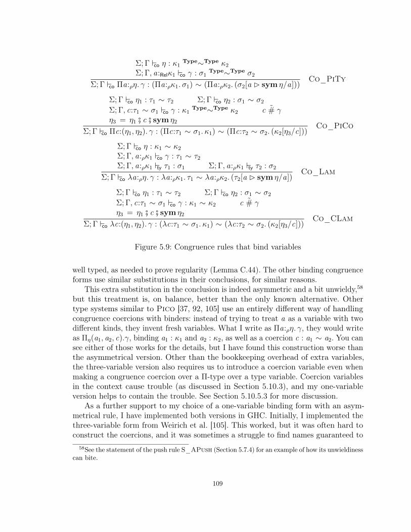
Σ; Γ co η : κ1Type∼Type κ2

Σ; Γ, a:Relκ1 co γ : σ1Type∼Type σ2

Σ; Γ co Πa:ρη. γ : (Πa:ρκ1. σ1) ∼ (Πa:ρκ2. (σ2[a B sym η/a]))Co_PiTy

Σ; Γ co η1 : τ1 ∼ τ2 Σ; Γ co η2 : σ1 ∼ σ2

Σ; Γ, c:τ1 ∼ σ1 co γ : κ1Type∼Type κ2 c # γ

η3 = η1 # c # sym η2

Σ; Γ co Πc:(η1, η2). γ : (Πc:τ1 ∼ σ1. κ1) ∼ (Πc:τ2 ∼ σ2. (κ2[η3/c]))Co_PiCo

Σ; Γ co η : κ1 ∼ κ2

Σ; Γ, a:ρκ1 co γ : τ1 ∼ τ2

Σ; Γ, a:ρκ1 ty τ1 : σ1 Σ; Γ, a:ρκ1 ty τ2 : σ2

Σ; Γ co λa:ρη. γ : λa:ρκ1. τ1 ∼ λa:ρκ2. (τ2[a B sym η/a])Co_Lam

Σ; Γ co η1 : τ1 ∼ τ2 Σ; Γ co η2 : σ1 ∼ σ2

Σ; Γ, c:τ1 ∼ σ1 co γ : κ1 ∼ κ2 c # γη3 = η1 # c # sym η2

Σ; Γ co λc:(η1, η2). γ : (λc:τ1 ∼ σ1. κ1) ∼ (λc:τ2 ∼ σ2. (κ2[η3/c]))Co_CLam

Figure 5.9: Congruence rules that bind variables

well typed, as needed to prove regularity (Lemma C.44). The other binding congruenceforms use similar substitutions in their conclusions, for similar reasons.

This extra substitution in the conclusion is indeed asymmetric and a bit unwieldy,58

but this treatment is, on balance, better than the only known alternative. Othertype systems similar to Pico [37, 92, 105] use an entirely different way of handlingcongruence coercions with binders: instead of trying to treat a as a variable with twodifferent kinds, they invent fresh variables. What I write as Πa:ρη. γ, they would writeas Πη(a1, a2, c).γ, binding a1 : κ1 and a2 : κ2, as well as a coercion c : a1 ∼ a2. You cansee either of those works for the details, but I have found this construction worse thanthe asymmetrical version. Other than the bookkeeping overhead of extra variables,the three-variable version also requires us to introduce a coercion variable even whenmaking a congruence coercion over a Π-type over a type variable. Coercion variablesin the context cause trouble (as discussed in Section 5.10.3), and my one-variableversion helps to contain the trouble. See Section 5.10.5.3 for more discussion.

As a further support to my choice of a one-variable binding form with an asym-metrical rule, I have implemented both versions in GHC. Initially, I implemented thethree-variable form from Weirich et al. [105]. This worked, but it was often hard toconstruct the coercions, and it was sometimes a struggle to find names guaranteed to

58See the statement of the push rule S_APush (Section 5.7.4) for an example of how its unwieldinesscan bite.

109

be fresh. When I refactored the code to use the one-variable version formalized here,the code became simpler.

5.8.5.2 Congruence over coercion binders

The congruence forms over types that bind coercion variables (rules Co_PiCo andCo_CLam) have two more wrinkles. The first is that there is no equivalent ofCo_PiTy’s η coercion that relates two propositions; we must settle for the pair ofcoercions (η1, η2) that appear in Co_PiCo and Co_CLam. These coercions relatecorresponding parts of the propositions. The second wrinkle is in the c # γ premise ofboth of these rules.

Definition (“Almost devoid”). Define c # γ (pronounced “γ is almost devoid of c”)to mean that the coercion variable c appears nowhere in γ except, perhaps, in one ofthe types related by a τ1 ≈η τ2 coercion.

The almost-devoid condition on Co_PiCo and Co_CLam restricts where thebound variable c can appear in the coercion body. This technical restriction, basedon the original idea by Weirich et al. [105], is necessary for my proof of consistency(Section 5.10) to go through. The motivation for the restriction is discussed in depthin Section 5.10.3.

The key example that this restriction forbids looks like this:

Σ; Γ 6 co Πc:(〈Int〉, 〈Bool〉). c : (Πc:Int ∼ Bool . Int) ∼ (Πc:Int ∼ Bool .Bool)

It would seem that this coercion would not cause harm, yet I know of no way to proveconsistency while allowing it. See Section 5.10.5 for a discussion of other approaches.

Happily, this restriction is not likely to bite when translating Dependent Haskellprograms to Pico, as we can write functions witnessing the isomorphism between thetwo types related above:

to :˜Π(x :Rel(

˜Πc:Int ∼ Bool . Int)). (

˜Πc:Int ∼ Bool .Bool)

to =λ(x :Rel(˜Πc:Int ∼ Bool . Int)), (c:Int ∼ Bool). (x c)B c

from :˜Π(x :Rel(

˜Πc:Int ∼ Bool .Bool)). (

˜Πc:Int ∼ Bool . Int)

from=λ(x :Rel(˜Πc:Int ∼ Bool .Bool)), (c:Int ∼ Bool). (x c)B sym c

A compiler of Dependent Haskell creates functions such as these as it is compilinga subsumption relationship ≤, as discussed further in Section 6.4.2. In other words,while we don’t have (Πc:Int ∼ Bool . Int) ∼ (Πc:Int ∼ Bool .Bool), these two typesare related by ≤, in both directions. This mean that a Dependent Haskell programthat expects one of these types in a certain context, but gets the other type, is stillwell typed.

When can the lack of the equality proof bite? Only when that proof is needed as acoercion argument to some function or GADT constructor. As we’ve just seen, using

110

it to cast is unnecessary, as we can just use one component of the isomorphism. Theforbidden equalities all relate Π-types over coercions. Yet, in Dependent Haskell, anabstraction over an equality constraint is considered a polytype. Passing a polytypeas an argument is considered a use of impredicativity, which is not supported. (SeeSection 4.4.4.) In particular, the equality constraint ((Int ∼ Bool)⇒ Int) ∼ ((Int ∼Bool) ⇒ Bool) is malformed in Dependent Haskell, because it passes polytypes asarguments to ∼ . I thus conjecture that no Dependent Haskell program is ruled outbecause of the coercion variable restriction. Proving such a claim seems challenging,however, and remains as an exercise for the reader.

5.8.5.3 (Almost) Congruence

The coercion variable restriction means that equality is not quite congruent, accordingto the following definition:

Definition (Congruence). Equality is congruent if, whenever Σ; Γ co γ : σ1κ∼κ σ2 and

Σ; Γ, a:ρκ ty τ : κ0, there exists η such that Σ; Γ co η : τ [σ1/a] κ0[σ1/a]∼κ0[σ2/a] τ [σ2/a].

If we were to try to prove that equality is congruent, it seems natural to proceedby induction on the typing derivation for τ . However, in the proof, we are stuck whenτ = λc:φ. τ0. The congruence form for λ-types over coercions is no help because of thecoercion variable restriction.59 If we strengthen the induction hypothesis to providewhat we need in this case, then other cases fail, unable to obey the restriction.

As a concrete example, consider this: Let Γ = y :RelInt, c:3 ∼ y and τ = λ(c ′:Int ∼Bool). xBc ′. We know Σ; Γ co c : 3 ∼ y and Σ; Γ, x :RelInt ty τ :

˜Π(c′:Int ∼ Bool).Bool .

Yet there seems to be no way to construct a proof of τ [3/x ] ∼ τ [y/x ].60

Instead of proving congruence, I am left proving almost-congruence, as follows:

Definition (Unrestricted coercion variables [Definition C.87]). Define a new judgment∗co to be identical to co, except with the c # γ premises removed from rules Co_PiCoand Co_CLam and all recursive uses of co replaced with ∗

co.

Now, the proof for the following theorem is straightforward:

Theorem ((Almost) Congruence [Theorem C.90]). Equality is congruent with thejudgment ∗co.

59Contrast to the proof of the lifting lemma in my prior work [106]; that proof relies on a criticalauxiliary lemma (their Lemma C.7) which requires a different coercion variable restriction than whatI am using here. Furthermore, I show in Section 5.10.5.2 that their restriction is too weak.

60It is tempting to try to prove this by using the Co_CLam form and then coherence formsstitched together with transitivity; after all, the c # γ restriction in Co_CLam does not affect thetypes in a coherence coercion. However, the η coercion in the coherence coercion (η relates the kindsof the types mentioned in the coherence coercion) must still be devoid of c, and that is where thisplan falls apart.

111

What this means, in practice, is that we can often think of equality as congruent,and intuition about the equality relation stemming from congruence is often accurate.In particular, if the type τ in the statement of congruence has no coercion abstractionsor Π-types, then congruence with respect to co holds.61

5.8.5.4 Consequences of congruence

Congruence is not, thankfully, a necessary property of Pico. Nowhere in the metatheorydo we rely on this result (or lack thereof).

In the implementation, however, congruence62 is used to perform some coercionoptimizations [96]. After desugaring Haskell into its Core language (currently basedon the version of System FC as described in my prior work [105]), GHC optionallyperforms coercion optimization, in the hope of converting large coercions into smallerones that prove the same propositions. This speeds up compilation and reduces thesize of the interface files that GHC writes to disk to store information about compiledmodules; the optimization has no effect at runtime, however, because coercions arefully erased before execution.

Congruence comes into play when optimizing a coercion such as (Πa:ρη. γ1)@γ2,where γ1@γ2 is a decomposition form that instantiates a Π-type (Section 5.8.6.2).Without going into further detail, in order to perform the instantiation requested, wemust find exactly the coercion suggested in the definition of congruence above. SincePico lacks congruence, the updated coercion optimizer sometimes fails to optimizethese coercions. The troublesome case—when we would run afoul of the c # γrestrictions in Co_PiCo and Co_CLam—is easy to detect, and the optimization issimply skipped when this were to happen. The lack of congruence does not otherwisebite.

5.8.6 Equality can be decomposed

Pico comes equipped with a large variety of ways of decomposing an equality to getout a smaller one—in some sense, these are the inverses of the congruence forms. Wewill approach these in batches.

5.8.6.1 The argk forms

The coercion form argk extracts a coercion between the kinds of the bound variablesin a coercion relating abstractions. The rules appear in Figure 5.10 on the next page.The rules are actually straightforward; look at Co_ArgK for a typical example. Thisform extracts the equality between κ1 and κ2 from the type of γ. The other forms work

61This intuition is hard to state precisely, because of the possibility that the contexts have abstrac-tions over coercions. We would somehow need a premise that states that no coercion abstractions are“reachable” from τ , but defining such a property and then proving this claim seems not to pay its way.

62What I call congruence here has been called the lifting lemma in the literature.

112

Σ; Γ co γ : (Πa:ρκ1. σ1) ∼ (Πa:ρκ2. σ2)

Σ; Γ co argk γ : κ1 ∼ κ2

Co_ArgK

Σ; Γ co γ : (Πc:(τ1 ∼ τ ′1). σ1) ∼ (Πc:(τ2 ∼ τ ′2). σ2)

Σ; Γ co argk1 γ : τ1 ∼ τ2

Co_CArgK1

Σ; Γ co γ : (Πc:(τ1 ∼ τ ′1). σ1) ∼ (Πc:(τ2 ∼ τ ′2). σ2)

Σ; Γ co argk2 γ : τ ′1 ∼ τ ′2Co_CArgK2

Σ; Γ co γ : (λa:ρκ1. σ1) ∼ (λa:ρκ2. σ2)

Σ; Γ co argk γ : κ1 ∼ κ2

Co_ArgKLam

Σ; Γ co γ : (λc:(τ1 ∼ τ ′1). σ1) ∼ (λc:(τ2 ∼ τ ′2). σ2)

Σ; Γ co argk1 γ : τ1 ∼ τ2

Co_CArgKLam1

Σ; Γ co γ : (λc:(τ1 ∼ τ ′1). σ1) ∼ (λc:(τ2 ∼ τ ′2). σ2)

Σ; Γ co argk2 γ : τ ′1 ∼ τ ′2Co_CArgKLam2

Figure 5.10: The argk rules of coercion formation

analogously. The forms with argki are necessary because Pico has no built-in notionof an equality between equalities: If we tried to extract a relation between propositionslike we do in Co_ArgK, we would need something that looks like φ1 ∼ φ2, whichdoes not exist in Pico. So, we have to extract either the left side of the propositionsor the right side.

Note that these rules are syntax-directed even though their conclusions overlap:we can always find the proposition a coercion proves and then decide which argk ruleto use.

5.8.6.2 The instantiation forms

Given a coercion between abstractions, we can instantiate the bound variable andget a coercion between the instantiated bodies. The rules for these coercions are inFigure 5.11 on the following page.

These rules are essentially concrete instances of two rule schemas, one for instanti-ation coercions built with @, and the other for “result” coercions built with res. Theinstantiation coercions can work with one of three argument types (relevant type,irrelevant type, and coercion) and one of two forms (Π and λ), leading to six verysimilar rules. Along the same lines, res coercions work with both Π and λ, thoughthis form is agnostic to the argument flavor, so we get only two rules.

The instantiation coercions are essential in writing the push rules (Section 5.7.4)

113

Σ; Γ co γ : Πa:Relκ1. σ1 ∼ Πa:Relκ2. σ2

Σ; Γ co η : τ1κ1∼κ2 τ2

Σ; Γ co γ@η : σ1[τ1/a] ∼ σ2[τ2/a]Co_InstRel

Σ; Γ co γ : Πa:Irrelκ1. σ1 ∼ Πa:Irrelκ2. σ2

Σ; Γ co η : τ1κ1∼κ2 τ2

Σ; Γ co γ@η : σ1[τ1/a] ∼ σ2[τ2/a]Co_InstIrrel

Σ; Γ co η1 : Πc:φ1. σ1 ∼ Πc:φ2. σ2

Σ; Γ co γ1 : φ1 Σ; Γ co γ2 : φ2

Σ; Γ co η1@(γ1, γ2) : σ1[γ1/c] ∼ σ2[γ2/c]Co_CInst

Σ; Γ co γ : λa:Relκ1. τ1 ∼ λa:Relκ2. τ2

Σ; Γ co η : σ1κ1∼κ2 σ2

Σ; Γ co γ@η : τ1[σ1/a] ∼ τ2[σ2/a]Co_InstLamRel

Σ; Γ co γ : λa:Irrelκ1. τ1 ∼ λa:Irrelκ2. τ2

Σ; Γ co η : σ1κ1∼κ2 σ2

Σ; Γ co γ@η : τ1[σ1/a] ∼ τ2[σ2/a]Co_InstLamIrrel

Σ; Γ co γ : λc:φ1. σ1 ∼ λc:φ2. σ2

Σ; Γ co η1 : φ1 Σ; Γ co η2 : φ2

Σ; Γ co γ@(η1, η2) : σ1[η1/c] ∼ σ2[η2/c]Co_CInstLam

Σ; Γ co γ : ?Π∆1. τ1 ∼ ?Π∆2. τ2 |∆1| = |∆2| = nΣ; Γ ty τ1 : Type Σ; Γ ty τ2 : Type

Σ; Γ co resn γ : τ1 ∼ τ2

Co_Res

Σ; Γ co γ : λ∆1. τ1 ∼ λ∆2. τ2 |∆1| = |∆2| = nΣ; Γ ty τ1 : κ1 Σ; Γ ty τ2 : κ2

Σ; Γ co resn γ : τ1 ∼ τ2

Co_ResLam

Figure 5.11: Instantiation rules of coercion formation

114

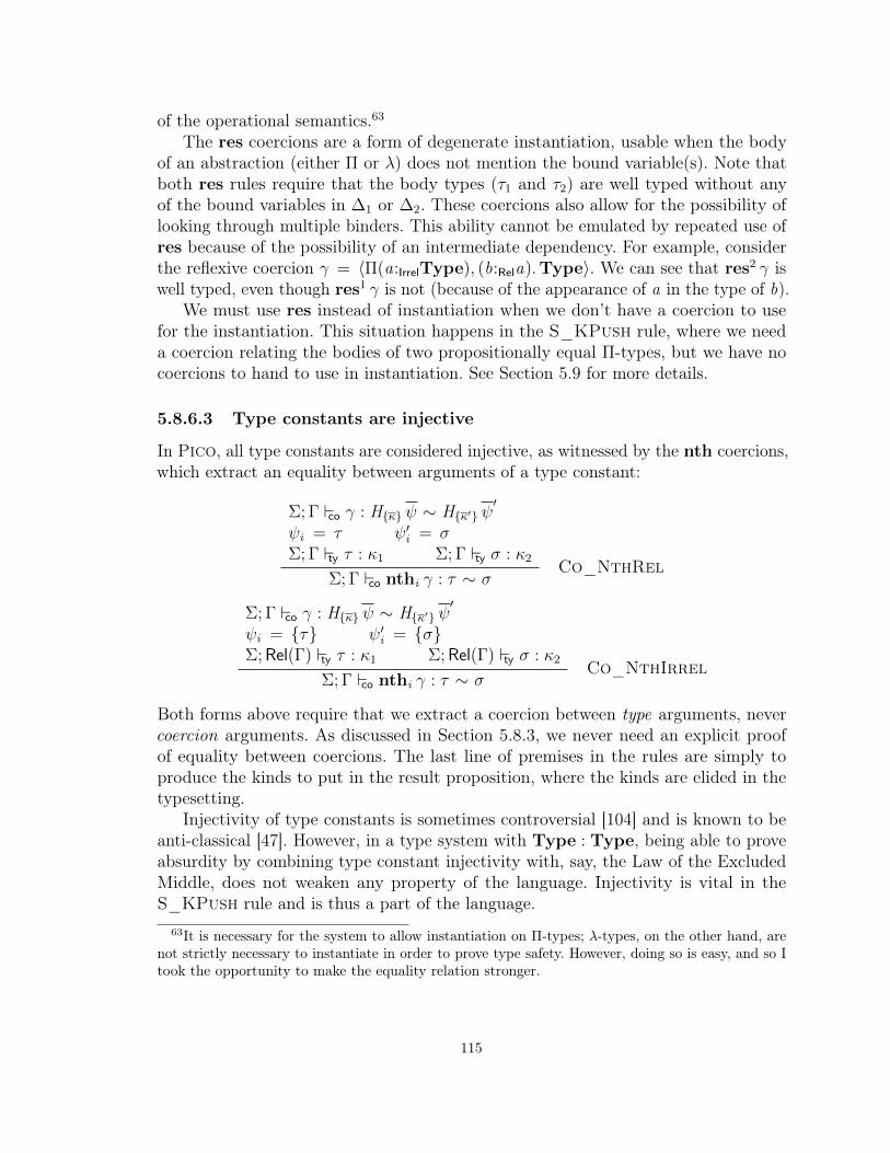
of the operational semantics.63

The res coercions are a form of degenerate instantiation, usable when the bodyof an abstraction (either Π or λ) does not mention the bound variable(s). Note thatboth res rules require that the body types (τ1 and τ2) are well typed without anyof the bound variables in ∆1 or ∆2. These coercions also allow for the possibility oflooking through multiple binders. This ability cannot be emulated by repeated use ofres because of the possibility of an intermediate dependency. For example, considerthe reflexive coercion γ = 〈Π(a:IrrelType), (b:Rela).Type〉. We can see that res2 γ iswell typed, even though res1 γ is not (because of the appearance of a in the type of b).

We must use res instead of instantiation when we don’t have a coercion to usefor the instantiation. This situation happens in the S_KPush rule, where we needa coercion relating the bodies of two propositionally equal Π-types, but we have nocoercions to hand to use in instantiation. See Section 5.9 for more details.

5.8.6.3 Type constants are injective

In Pico, all type constants are considered injective, as witnessed by the nth coercions,which extract an equality between arguments of a type constant:

Σ; Γ co γ : Hκ ψ ∼ Hκ′ ψ′

ψi = τ ψ′i = σΣ; Γ ty τ : κ1 Σ; Γ ty σ : κ2

Σ; Γ co nthi γ : τ ∼ σCo_NthRel

Σ; Γ co γ : Hκ ψ ∼ Hκ′ ψ′

ψi = τ ψ′i = σΣ; Rel(Γ) ty τ : κ1 Σ; Rel(Γ) ty σ : κ2

Σ; Γ co nthi γ : τ ∼ σCo_NthIrrel

Both forms above require that we extract a coercion between type arguments, nevercoercion arguments. As discussed in Section 5.8.3, we never need an explicit proofof equality between coercions. The last line of premises in the rules are simply toproduce the kinds to put in the result proposition, where the kinds are elided in thetypesetting.

Injectivity of type constants is sometimes controversial [104] and is known to beanti-classical [47]. However, in a type system with Type : Type, being able to proveabsurdity by combining type constant injectivity with, say, the Law of the ExcludedMiddle, does not weaken any property of the language. Injectivity is vital in theS_KPush rule and is thus a part of the language.

63It is necessary for the system to allow instantiation on Π-types; λ-types, on the other hand, arenot strictly necessary to instantiate in order to prove type safety. However, doing so is easy, and so Itook the opportunity to make the equality relation stronger.

115

Σ; Γ co γ : τ1 ψ1 ∼ τ2 ψ2

Σ; Γ ty τ1 : ’Πδ1. κ1 Σ; Γ ty τ2 : ’Πδ2. κ2

Σ; Γ co η : ’Πδ1. κ1 ∼ ’Πδ2. κ2

Σ; Γ co leftη γ : τ1 ∼ τ2

Co_Left

Σ; Γ co γ : τ1 σ1 ∼ τ2 σ2

Σ; Γ ty σ1 : κ1 Σ; Γ ty σ2 : κ2 Σ; Γ co η : κ1 ∼ κ2

Σ; Γ co rightη γ : σ1 ∼ σ2

Co_RightRel

Σ; Γ co γ : τ1 σ1 ∼ τ2 σ2Σ; Γ ty σ1 : κ1 Σ; Γ ty σ2 : κ2 Σ; Γ co η : κ1 ∼ κ2

Σ; Γ co rightη γ : σ1 ∼ σ2

Co_RightIrrel

Figure 5.12: Function application decomposition coercions

5.8.6.4 Matchable types are generative and injective

In Section 4.2.4, I define matchable as the conjunction of generative and injective. Picoincludes two coercion forms that witness the generativity (left) and injectivity (right)of matchable function types, as shown in Figure 5.12. Note that the applications in theproposition proved by γ are matchable applications τ ψ, distinct from unmatchableapplications τ˜ψ.Interestingly, these coercions require an extra coercion η that proves that the kindsof the output types are equal. This kind coercion is necessary to prove the consistencyof the kind coercion (Section 5.8.1). It is curiously absent from my prior work on kindequalities [105], but I now believe that this coercion is necessary—though I have yet tofind a counterexample to consistency by omitting it, I am unable to prove consistencywithout it.

Does adding this extra argument to left and right now weaken Pico’s expressive-ness, compared to its predecessors? Yes and no:

Yes, fewer coercions are available, when comparing against the system in myprior work [105]. However, I argue in Section 5.10.5.2 that the proof in that priorwork is broken, precisely around its kind coercion. If Pico reduces expressivenesscompared to an unsound system, this may be an improvement.

No fewer coercions are available, when comparing against the System FC beforekind equalities (that is, the System FC in GHC 7). Prior to GHC 8, the leftand right coercions required the kinds of the output types to be identical. Inthose cases, the η coercion in Pico’s left and right would just be reflexive.Though this restriction on the kinds was overlooked in the original publication

116

on System FC [87], it appears in later treatments [11, 32].64

I thus conclude that adding these extra kind coercions is appropriate, considering thattheir omission in GHC 8.0 may be unsafe and that including them is conservativewith respect to GHC 7.

5.8.7 Equality includes β-reduction

The last rule to consider in the co judgment is the one that witnesses β-reduction:

Σ; Γ ty τ : κ Σ; Γ ty τ′ : κ

Σ; Γ s τ −→ τ ′

Σ; Γ co step τ : τ ∼ τ ′Co_Step

This rule is in place of having β-equivalence be part of definitional equality, asis done in some other dependently typed languages, such as Coq. Instead, in orderto get a type to reduce, a Pico program must invoke the step coercion explicitly.Generating these coercions is quite painful to do by hand (as seen in the example inSection 5.5.3), but straightforward for a compiler.65

You will see that the rule requires both the redex and the reduct to be well kindedat kind κ. The requirement on the reduct is implied by the preservation theorem(Theorem C.46), but omitting it from the rule means that the proofs of propositionregularity (Lemma C.44) and preservation would have to be mutually inductive. Itseems simpler just to add this extra, redundant premise.

5.8.8 Discussion

The coercion language in Pico is quite extensive, boasting (or suffering from, dependingon your viewpoint) 37 separate typing rules. I consider here, briefly, why this is so.

There are several coercion forms (to wit, 10) that are absolutely essential for Picoto be proven type-safe and yet remain meaningful. These include the equivalence andcoherence rules, assumptions, the Π-congruence form over type variables,66 argk overΠ, instantiation over Π, injectivity, and β-reduction. With the exception of assumptions(Co_Var) and β-reduction (Co_Step), these forms are all needed somewhere in thepush rules (Section 5.7.4).67 Assumptions and β-reduction, however, make Pico what

64The left and right coercions were omitted entirely from Yorgey et al. [107]. Correspondingly,they were dropped from the implementation in GHC 7.4. However, users found that this omissionprevented some programs from being accepted. See GHC ticket #7205.

65If a type must reduce many times, it would be more efficient to support a stepn coercion formthat performs n steps at once. Indeed, this is what I plan to implement. It is easier, however, toprove properties about single-step reduction.

66This form is needed only to support reduction under irrelevant λs.67I am considering here a version of Pico without unsaturated matches. If we wish to include

unsaturated matches, we would also need res over Π.

117

it is; the language would be near useless as a candidate for an internal dependentlytyped language without these.

The rest of the forms merely enrich the equality relation, while remaining inessential.I have decided to include them to make the equality relation relate more types. Doingso makes Pico—and, in turn, Dependent Haskell—more expressive. When addingrules, we must be careful that the new forms do not violate consistency (or otherproved properties), so they are not entirely free. Perhaps there are more useful, saferules one could add later, simply by updating the relevant proofs. Because Piconever inspects the structure of a coercion, adding new rules introduces only a minimalburden on any implementation—essentially just for bookkeeping. I thus leave openthe possibility of more coercions as Pico gets used in practice.

5.9 The S_KPush rule

Σ tc H : a:Irrelκ; ∆;H ′ ∆ = ∆1,∆2 n = |∆2|κ = ’Πa:Irrelκ,∆.H

′ a

σ = ’Π(∆2[τ/a][ψ/dom(∆1)]).H ′ τ

σ′ = ’Π(∆2[τ ′/a][ψ′/dom(∆1)]).H ′ τ ′

Σ; Rel(Γ) co η : σ ∼ σ′

Σ; Rel(Γ) vec τ′ : a:Relκ

∀i , γi = build_kpush_co(〈κ〉@(nths (resn η));ψ1...i−1)∀i , ψ′i = cast_kpush_arg(ψi ; γi)

H → κ′ ∈ alt

Σ; Γ s caseκ0 (Hτ ψ)B η of alt −→ caseκ0 Hτ ′ ψ′of alt

S_KPush

The S_KPush rule handles the case where the scrutinee of a case expression isheaded by a cast. As in all previous work on System FC, this push rule is the mostintricate. However, in this dissertation, I have taken a new approach to S_KPushthat does not require the so-called “lifting lemma” of previous work.68 This liftinglemma is a generalization of the congruence property, which does not hold in Pico(Section 5.8.5.3). Instead, I rely on instantiating the type of a type constant, and onthe fact that type constant types are always closed. As the computational contentof the S_KPush rule must actually be implemented as part of a compiler that usesPico, this (slightly) simpler statement of S_KPush may prove to be a measurableoptimization in practice.

A few examples can demonstrate the general idea. Firstly, note that in S_KPush,only the scrutinee matters; the alternatives remain the same before and after thereduction. With that in mind, we can see scrutinees before and after pushing inFigure 5.13 on the following page.

68See for example, Weirich et al. [105], which contains a good, detailed explication of the liftinglemma.

118

Original scrutinee Assumptions / NotesPushed scrutineeTrue B 〈Bool〉 simple case; no universals (1)True

JustInt 3B γ Σ; Γ co γ : Maybe Int ∼ Maybe bb:IrrelType ∈ Γ

(2)

Justb (3B argk (〈’Πa:IrrelType, x :Rela.Maybe a〉@(nth1 γ)))

MkG Bool 〈Bool〉B γ Σ; Γ co γ : G Bool ∼ G bb:IrrelType ∈ Γ

(3)

MkG b (sym (argk1 η) # 〈Bool〉 # argk2 η), whereη = 〈’Π(a:IrrelType), (c:a ∼ Bool).G a〉@(nth1 γ)

(PackBool True MkPBool ,True)B γ Σ; Γ co γ : ’Πδ1.Ex Bool ∼ ’Πδ2.Ex bδ1 = y :RelProxy Bool Trueδ2 = y :RelProxy b (True B γ2)Σ; Γ co γ2 : Bool ∼ bb:IrrelType ∈ Γ

(4)

Packb True B η′0 (MkPBool ,True B η′1), whereκ = ’Π(k :IrrelType), (a:Irrelk), (x :RelProxy k a), (y :RelProxy k a).Ex kη0 = 〈κ〉@(nth1 (res1 γ))η′0 = argk η0

η1 = η0@(True ≈η′0 True B η′0)

η′1 = argk η1

The reductions above assume the following datatypes. In Haskell:

data Bool = False | Truedata Maybe a = Just a | Nothingdata G a whereMkG :: G Bool

data Proxy (a :: k) = MkPdata Ex k wherePack :: ∀ (a :: k). Proxy a→ Proxy a→ Ex k

And in Pico:

Σ =Bool :(∅),False:(∅;Bool),True:(∅;Bool)Maybe:(a:Type), Just:(x :Rela;Maybe),Nothing :(∅;Maybe)G :(a:Type),MkG :(c:a ∼ Bool ;G )Proxy :(k : Type, a : k),MkP :(∅;Proxy)Ex :(k :Type),Pack :(a:Irrelk , x :RelProxy k a, y :RelProxy k a;Ex)

Figure 5.13: Examples of S_KPush

119

build_kpush_co(γ;∅) = γ

build_kpush_co(γ;ψ, τ) = let c := build_kpush_co(γ;ψ) inc@(τ ≈argk c τ B argk c)

build_kpush_co(γ;ψ, τ) = let c := build_kpush_co(γ;ψ) inc@τ ≈argk c τ B argk c

build_kpush_co(γ;ψ, η) = let c := build_kpush_co(γ;ψ) inc@(η, sym (argk1 c) # η # argk2 c)

cast_kpush_arg(τ ; γ) = τ B argk γ

cast_kpush_arg(τ; γ) = τ B argk γcast_kpush_arg(γ; η) = sym (argk1 η) # γ # argk2 η

Figure 5.14: Helper functions implementing S_KPush

Example (1) In this example, there are no universals of the type in question (Bool),and so “pushing” is extraordinarily simple: just drop the coercion. We can see thisin terms of S_KPush in that both τ and ψ are empty. Note that if we had a non-reflexive coercion in the scrutinee—that is, if the scrutinee were, say, True B γ withΣ; Γ co γ : Bool ∼ a—the case expression would not be well typed. Rule Ty_Caserequires the type of a scrutinee to be of the form ’Π∆.H σ. The type a does nothave this form, and so such a scrutinee is disallowed. Also note that we cannot haveTrue B γ with Σ; Γ co γ : Bool ∼ Int due to the consistency lemma (Section 5.10).

Example (2) This is the simplest non-trivial example. We need to push a coercionγ proving Maybe Int ∼ Maybe b into JustInt 3. This coerced scrutinee has typeMaybe b; the pushed scrutinee must have the same type. We thus know it must startwith Justb. The only challenge left is to cast the argument, 3, with a coercion thatproves Int ∼ b. We will always be able to extract this coercion from the coercioncasting the scrutinee, γ. But how, in general?

The coercion needed to cast each (existential) argument to a constructor mustsurely depend on the type of the constructor. Previous versions of System FC dida transformation on this type to produce the coercion. In this work, I instantiatethe type using the @ operator (Section 5.8.6.2) via the helper metatheory functionsbuild_kpush_co and cast_kpush_arg, presented in Figure 5.14.

In the present case—pushing a coercion into Just : ’Πa:IrrelType, x :Rela.Maybe a—we take Just’s type and instantiate a by the coercion nth1 γ, which proves Int ∼ b.We are thus left with a coercion that proves

(’Πx :RelInt.Maybe Int) ∼ (’Πx :Relb.Maybe b).

120

bsym (argk1 η)−−−−−−−−→ Booly〈Bool〉

Bool ←−−−−−−−−argk2 η

Bool

Figure 5.15: “Casting” a coercion in Example (3)

Then, all we have to do is use argk to extract the coercion proving Int ∼ b and wecan use it to cast 3.

Seeing the above action in the definition for S_KPush may be challenging. Let’stake another look, focusing on the metavariables in the definition of the rule (presentedin Figure 5.7 on page 102). The type σ is the type of the underlying (uncoerced)scrutinee, and σ′ is the type of the coerced scrutinee. In our example, we haveσ = Maybe Int and σ′ = Maybe b. Note that neither of these are ’Π-types, and thusthe telescope ∆2 from the rule is empty, with n = 0. The κ metavariable in the ruleis the type of Just, above. The coercion we are building is the one to cast the firstargument, that is, γ1. The second argument to build_kpush_co is a list of all previousexistential arguments, but in our case, there are no previous arguments, so this list isempty. We thus have γ1 = build_kpush_co(〈κ〉@(nth1 γ);∅).69 We can see from thedefinition of build_kpush_co that the function just returns its first argument whenits second argument is empty, and so we get γ1 = 〈κ〉@(nth1 γ) as desired. The useof cast_kpush_arg is to apply the right argk form (Section 5.8.6.1), depending onwhether we are casting a type or “casting” a coercion.

We focus on understanding cast_kpush_arg on the next example.

Example (3) The datatype G is a simple-as-they-come GADT. In this example,we cast MkG :: G Bool to have type G b (for some type variable b). The action inS_KPush here is actually quite similar to the previous case, because MkG is quitesimilar to Just: both take one argument, whose type depends on the one universalparameter. The difference here is that MkG ’s argument is a coercion, whereas Just’s isa type. We thus cannot use argk in exactly the same way as before, instead requiringargk1 and argk2, as diagrammed in Figure 5.15. In this example, two of the steps inthe diagram are redundant, but they will not be, in general. It can be convenient tothink of constructions such as this as “casting” a coercion—that is, taking the coercion〈Bool〉 and changing it to connect b with Bool . Indeed, prior work [105] even used aspecial notation for this: γ B η1 ∼ η2, but I find it clearer to avoid the sugar.

69Technically, we should write res0 γ, because the superscript in res coercions is part of thelanguage, not the metatheory. However, a res0 coercion is a no-op, so I leave it out here for simplicity.

121

Example (4) Having warmed ourselves up on the simpler examples above, Example(4) demonstrates the full complexity of S_KPush, including dependent existentialarguments and an unsaturated scrutinee. We’ll take these complications one at a time.

Having dependent existentials motivates the intricacies of build_kpush_co. Sincethe pushed-in cast changes universal arguments (unless it’s reflexive), we need to castexistential arguments that may be dependent on the universals. However, if a laterexistential argument is dependent upon an earlier one and we change the earlier one,we must also change that later one. In this example, the first existential argument(instantiated to True) depends on the universal argument (instantiated to Bool), andthe second existential depends on the first. The first existential is cast by η′0 and thusthe second must be cast by η′1, which essentially replaces the occurrence of True in thetype of the applied MkP constructor with True B η′0, using a coherence coercion builtwith ≈. Indeed, this is the whole point of build_kpush_co—using coherence to alterthe types of later existentials depending on earlier ones. Here is the critical correctnessproperty of build_kpush_co:

Lemma (Correctness of build_kpush_co [Lemma C.45]).Assume Σ; Γ cev ψ : ∆[τ/a], and let γi = build_kpush_co(η;ψ1...i−1) and ψ′i =cast_kpush_arg(ψi ; γi). If Σ; Rel(Γ) co η : (’Π∆. σ)[τ/a] ∼ (’Π∆. σ)[τ ′/a], then:

1. Σ; Rel(Γ) co build_kpush_co(η;ψ) : σ[τ/a][ψ/dom(∆)] ∼ σ[τ ′/a][ψ′/dom(∆)]

2. Σ; Γ cev ψ′: ∆[τ ′/a]

This lemma is phrased in terms of cev; that relation includes the same elements as vec

but allows induction from right-to-left instead of the usual left-to-right. The η in thelemma statement relates the type of a constructor to itself, but with the universalsinstantiated with potentially different concrete arguments. These instantiations comedirectly from the coercion being pushed into the scrutinee, by way of nth. (Note thatthe ’Π quantifiers in the type of η above are not a consequence of the possibility ofunsaturation; instead, these are the existentials of the data constructor.) The lemmaconcludes that the resulting coercion relates the instantiated coercion (that is, theone built by build_kpush_co) to itself, with substitutions for both the universals andsome existentials. Along the way, it also asserts the validity of the cast existentials,via the cev result.

The remaining detail of Example (4) is its unsaturation. This is handled moresimply by a res coercion (Section 5.8.6.2), which looks through binders to relate thebodies of two abstract types. Indeed, S_KPush is the reason that the res coercionexists at all, though it is not a burden to support in the metatheory.

5.10 Metatheory: ConsistencyBroadly speaking, the type safety proof proceeds along lines well established by priorwork [11, 31, 106]. Indeed, the only challenge in proving the preservation theorem

122

τ1 ∝ τ2 Type compatibility

τ1 is not a valueτ1 ∝ τ2

C_NonValue1

τ2 is not a valueτ1 ∝ τ2

C_NonValue2

Hτ ψ ∝ Hτ ′ ψ′ C_TyCon

τ ∝ τ ′

Πa:ρκ. τ ∝ Πa:ρκ′. τ ′C_PiTy

Πc:φ. τ ∝ Πc:φ′. τ ′C_PiCo

λδ. τ ∝ λδ′. τ ′C_Lam

Figure 5.16: Type compatibility

is in dealing with S_KPush. The tricky bit is all in proving the correctness ofbuild_kpush_co; see Section 5.9. Otherwise, the proof of preservation is as expected.

On the other hand, progress is a challenge, as it has been in previous proofs oftype safety of System FC. We proceed, as before, by proving consistency and thenusing that to prove progress. (The definition for ∝ is in the next subsection.)

Lemma (Consistency [Lemma C.74]). If Γ contains only irrelevant type variablebindings and Σ; Γ co γ : τ1 ∼ τ2 then τ1 ∝ τ2.

We restrict Γ not to have any coercion variables bound. Otherwise, a coercionassumption might relate, say, Int and Bool and we would be unable to prove consistency.As consistency is needed only during the progress proof, this restriction does not posea problem.

5.10.1 Compatibility

The statement of consistency depends on the τ1 ∝ τ2 relation (pronounced “τ1 iscompatible with τ2”), as given in Figure 5.16. The goal of compatibility is to relateany two values (as defined in Section 5.7.1) that have the same head; non-valuesare compatible with everything. Note, in particular, in C_TyCon, that we careonly that the two H are the same. The universals (τ/τ ′) and existentials (ψ/ψ′) areallowed to differ. The one exception to this general scheme is in the C_PiTy rule,where we require the bodies τ/τ ′ also to be compatible. This is necessary becauseirrelevant binders are erased, and we must thus be sure that any exposed types arealso compatible.

123

Consistency is used in the progress proof mainly in order to establish the typingpremises of the push rules (Section 5.7.4). A representative example is in the casewhen we are trying to show that an application τ1 τ2 is either a value or can step (it isclearly not a coerced value; recall the statement of the progress theorem from Section5.7). The induction hypothesis tells us that τ1 is a value, a coerced value, or can step.If it can step, we are done by S_App_Cong. If τ1 is a value, we can determine thatit is a λ-abstraction and thus we can do β-reduction. The remaining case is when τ1 isa coerced value v B γ. We need to be able to show that γ relates two Π-types in orderto use S_PushRel. The right-hand type must be a Π-type because it is the functionin an application. But the only way we can show that the left-hand type is a Π-typeis by appealing to consistency.

We know, at this point, that the type being coerced is a value; thus its type is alsoa value (Lemma C.76, also introduced in Section 5.7.1). At this point, now that weknow that both types involved in the type of the coercion γ are values, compatibilitybecomes a much stronger definition, allowing us to conclude that if the types arecompatible and if one is a Π-type, the other must surely also be a Π-type. Because wecan rule out non-values in the places where we wish to invoke the consistency lemma,the flexibility around non-values does not get in our way.

5.10.2 The parallel rewrite relation

To prove consistency, I (following prior work) define a parallel rewrite relation, writtenτ1 τ2, and show that this relation includes pairs of compatible types only. A smallwrinkle with this definition is that the rewrite relation works over only types whosecoercions have been erased, as per the b·c operation, initially introduced along withcoherence coercions in Section 5.8.3. The operation, as you may recall, removes allcasts from a type, and replaces coercion arguments with an uninformative •. Strippingout casts and coercions is important in the rewrite relation; if the rewrite relationconsidered these features, the language would lose its coherence property. Goingforward, I use a convention where all types written as being related by have hadtheir coercions erased.

The rewrite relation appears in Figure 5.17 on the next page and Figure 5.18on page 126. Following conventions in the rewriting literature, I write τ1 τ3 τ2 tomean that τ1 τ3 and τ2 τ3, and I write τ1 ∗ τ2 to mean the reflexive, transitiveclosure of .

Note the Beta rules, which work over only unmatchable applications τ˜ψ. Thisfact allows us to conclude that matchable applications τ ψ never undergo β-reduction,in turn allowing us to prove that the left and right coercions are sound.

124

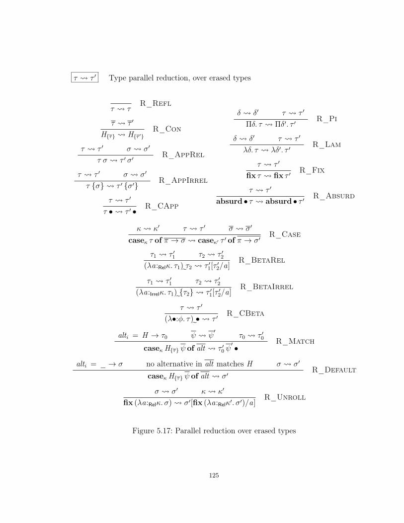
τ τ ′ Type parallel reduction, over erased types

τ τR_Refl

τ τ ′

Hτ Hτ ′R_Con

τ τ ′ σ σ′

τ σ τ ′ σ′R_AppRel

τ τ ′ σ σ′

τ σ τ ′ σ′R_AppIrrel

τ τ ′

τ • τ ′ •R_CApp

δ δ′ τ τ ′

Πδ. τ Πδ′. τ ′R_Pi

δ δ′ τ τ ′

λδ. τ λδ′. τ ′R_Lam

τ τ ′

fix τ fix τ ′R_Fix

τ τ ′

absurd • τ absurd • τ ′R_Absurd

κ κ′ τ τ ′ σ σ′

caseκ τ of π → σ caseκ′ τ ′ of π → σ′R_Case

τ1 τ ′1 τ2 τ ′2(λa:Relκ. τ1)˜τ2 τ ′1[τ ′2/a]

R_BetaRel

τ1 τ ′1 τ2 τ ′2(λa:Irrelκ. τ1)˜τ2 τ ′1[τ ′2/a]

R_BetaIrrel

τ τ ′

(λ•:φ. τ)˜• τ ′R_CBeta

alti = H → τ0 ψ ψ′

τ0 τ ′0

caseκHτ ψ of alt τ ′0 ψ′ •

R_Match

alti = _→ σ no alternative in alt matches H σ σ′

caseκHτ ψ of alt σ′R_Default

σ σ′ κ κ′

fix (λa:Relκ. σ) σ′[fix (λa:Relκ′. σ′)/a]R_Unroll

Figure 5.17: Parallel reduction over erased types

125

δ δ′ Parallel reduction of binders

κ κ′

a:ρκ a:ρκ′R_TyBinder

τ τ ′ κ1 κ′1 κ2 κ′2 σ σ′

•:τ κ1∼κ2 σ •:τ ′ κ′1∼κ′2 σ′R_CoBinder

γ γ′ “Reduction” of erased coercion

• •R_ErasedCo

Figure 5.18: Parallel reduction auxiliary relations

5.10.2.1 Substitution

The relation is almost a non-deterministic, strong version of normal reduction(Σ; Γ s τ −→ τ ′). In all the congruence forms (toward the top of Figure 5.17 on theprevious page), the relation definition recurs in every component, as necessary tosupport the following lemma:

Lemma (Parallel reduction substitution in parallel [Lemma C.51]). Assume ψ ψ′.

1. If τ1 τ2, then τ1[ψ/z ] τ2[ψ′/z ].

2. If δ1 δ2, then δ1[ψ/z ] δ2[ψ′/z ].

Note that all of the reductions are single-step.Beyond the congruence rules, the rewrite relation includes parallel variants of

the reduction rules from the normal step relation, toward the bottom of the figure.Note that these allow the components of a type to step as the reduction happens, asrequired for the local diamond lemma needed to prove confluence.

5.10.2.2 Confluence

This reduction relation is confluent (that is, has the Church-Rosser property). I provethis by proving a local diamond lemma:

Lemma (Local diamond [Lemma C.54]).

1. If τ0 τ1 and τ0 τ2, then there exists τ3 such that τ1 τ3 τ2.

2. If δ0 δ1 and δ0 δ2, then there exists δ3 such that δ1 δ3 δ2.

The proof of this lemma reasons by induction on the structure of τ0/δ0 and makesheavy use of the substitution lemma above. It is not otherwise challenging. The localdiamond lemma implies confluence.

126

5.10.3 Completeness of the rewrite relation

Having written a confluent rewrite relation, we must also connect this relation to ourequality relation. This is done via the following lemma:

Lemma (Completeness of type reduction [Lemma C.62]). If Σ; Γ co γ : τ1κ1∼κ2 τ2

and c # γ for every c:φ ∈ Γ, then:

1. There exists some erased type ε such that bτ1c ∗ ε ∗ bτ2c.

2. There exists some erased type ε such that bκ1c ∗ ε ∗ bκ2c.

Both the statement and proof of this lemma are rather more challenging thanthe previous ones. The proof proceeds by induction on the typing derivation. It isnecessary in the proof to use the induction hypothesis on a premise where the contextΓ is extended with a coercion variable (say, in the case for Co_PiCo). Thus, eventhough we will only use this lemma in a context with no coercion variables, we muststrengthen the induction hypothesis to allow for coercion variables. Critically, though,we restrict how all coercion variables in the context can appear in γ, according to thedefinition of #, introduced in Section 5.8.5.2. This restriction allows us to skip theimpossible Co_Var case while still allowing induction in the Co_PiCo case.

The definition of c # γ allows c to appear in the types related by a coherence ≈coercion. Happily, in the Co_Coherence case (when proving clause 1 of the lemma),we do not need to use the induction hypothesis, as a premise of Co_Coherencestates that the erased types are, in fact, already equal. It is for precisely this reasonthat c # γ can allow c in the types in a coherence coercion.

We also see that the statement of the completeness lemma requires us to proveboth that the types are joinable under and also that the kinds are. Otherwise, therewould be no way to handle the kind case.

Having strengthened the induction hypothesis appropriately, the actual proof is nottoo hard. The case for transitivity uses confluence—this is the only place confluence isused. The decomposition forms use the fact that when a value type reduces under ,the reduct has to have the same shape as the redex, with individual components in theredex reducing to those same components in the reduct. To deal with step, we mustconsider the different possibilities given by the Σ; Γ s τ −→ τ ′ relation. The properreduction rules all have analogues in , the congruence rules all follow from theinduction hypothesis, and the push rules cause no change to a type with its coercionserased. To prove that the kinds are joinable, we must rely heavily on the deterministicnature of the typing relation, but there are no other undue complications.

5.10.4 From completeness to consistency

Having established the relationship between Σ; Γ co γ : φ and joinability with respectto the rewrite relation, we must only show that the rewrite relation relates compatibletypes. Here are the key lemmas:

127

Lemma (Joinable types are consistent [Lemma C.72]). If ε1 ∗ ε3 ∗ ε2, thenε1 ∝ ε2.

Lemma (Erasure/consistency [Lemma C.73]). If bτ1c ∝ bτ2c, then τ1 ∝ τ2.

Other than some care needed around irrelevant abstractions (which cause recursionin the rules defining ∝), these lemmas are not hard to prove.

With all the groundwork laid, we can now conclude our consistency lemma, statednear the top of this section.

5.10.5 Related consistency proofs

There are a few aspects of the consistency proof where it may be helpful to highlightthe differences between my proof here and those in prior work. The comments belowdispute other, published proofs of consistency. The authors of these proofs haveconceded to me in private communication that their proofs were incorrect and do notdisagree with my assertions here.

5.10.5.1 Non-linear, non-terminating rewrite systems are not confluent

As described in some detail by Eisenberg et al. [32], non-terminating rewrite systemswith non-linear left-hand sides are not confluent. We can easily see that the rewriterelation is not terminating. In this presentation, however, its “left-hand side” islinear. Breaking from previous work, I have phrased type families in Pico as λ-expressions that use case; thus the parallel to rewrite systems is not as apparent asin previous work. In the context of my work here, a non-linear left-hand side wouldlook like a primitive equality check, as further explored in Section 5.13.2. Because theformalization of Pico that I am presenting does not contain this equality operator, Iavoid the non-confluence problem described by Eisenberg et al. [32].

Nevertheless, promising new work in the term-rewriting community [50] suggeststhat there is a way to prove consistency without confluence even after adding anequality check. I leave it as future work to reconcile the approach here with the recentresult cited above.

5.10.5.2 The proof of consistency by Weirich et al. [105] is wrong

The type system presented in my prior work [105] is very similar to Pico, althoughwithout dependency. Its treatment of Co_PiCo is subtly different, however. Althoughthere are numerous changes in how the syntax is structured, that work effectivelyloosens the definition of c # γ to allow c anywhere in a coherence coercion (τ1 ≈η τ2).In contrast, Pico allows c only in τ1 or τ2, but not in η. When armed with the kindcoercion (identical in Pico to the version in the previous work), this allows us toviolate a key lemma used to prove consistency. Here is the counterexample coercion,translated into Pico:

128

γ =˜Πc:(〈Int〉, 〈Bool〉).kind (3 ≈c (3B c))

In the body of the abstraction, the coercion variable c has type Int ∼ Bool . Wecan use a coherence coercion to relate 3 and 3B c; their kinds are also related by c.We can then extract the kinds of the types related by the coherence coercion. Puttingit all together yields this fact:

Σ;∅ co γ : (˜Πc:Int ∼ Bool . Int) ∼ (

˜Πc:Int ∼ Bool .Bool)

The problem is that we can see that no rewrite relation will join the two types relatedby γ. Because the prior work’s type system permits γ, its consistency proof mustbe wrong. (Pico rules out γ for using c in an illegal spot—the kind coercion in thesubscript for ≈.) Note that the language in that work might indeed be consistent (Ihave no counterexample to consistency), but its consistency surely cannot be provedvia the use of a rewrite relation in the way presented in that paper.

5.10.5.3 A one-variable version of Co_PiTy simplifies the consistencyproof

Weirich et al.’s language differs along a different dimension, using three binders insteadof one in its version of Co_PiTy. (See discussion in Section 5.8.5.1.) Apart fromthe awkwardness of needing extra variable names, the three-binder approach posesanother problem: it introduces a coercion variable into the context. Unlike for theirCo_PiCo, Weirich et al. do not introduce a coercion variable restriction for thiscoercion variable, as it is always a proof of equality between two variables. This extracoercion variable cannot imperil consistency. To prove this in the consistency proof,Weirich et al. employ a notion of “Good” contexts, which must be threaded throughtheir proofs. My one-variable version, with no bound coercion variable, avoids thiscomplication.

5.10.5.4 The proof of consistency by Gundry [37] is wrong

Gundry, in his thesis, takes a very different approach to proving consistency ofhis evidence language, also closely related to Pico. He sets up, essentially, a step-indexed logical relation and uses it to consider only closed coercions; when, say, acoercion variable is added to the context, Gundry quantifies over all possible closingsubstitutions.

A key property of Gundry’s logical relation is transitivity. Yet, in his proof oftransitivity, the indices do not work out. Gundry was not able to spot a straightforwardsolution, and in unpublished work, Weirich also tackled this problem and failed. NeitherGundry nor Weirich (nor I) have a proof that the step-indexed logical relation approachis not able to work, but no one has been able to finish the proof, either.

The failure of this approach is disappointing, because Gundry’s evidence language

129

does not have the coercion variable restriction inherent in Pico’s Co_PiCo rule.Gundry’s language thus allows more coercions than does Pico.

Can a System-FC-like language be proven consistent without a coercion variablerestriction on its analogue of Co_PiCo? My personal belief is “yes”—given that Ibelieve such a language is, in fact, consistent—but researchers have yet to show it.

5.11 Metatheory: Type erasureA critical property of any intermediate language used to compile Haskell is its ability tosupport type erasure. Haskell takes pride in erasing all of its complicated, helpful typesbefore runtime, and the intermediate language must show that this is possible. Picoachieves this goal through its relevance annotations, where irrelevant abstractionsand applications can be erased. In previous, non-dependent intermediate languagesfor Haskell, irrelevant abstractions and applications were also erased, but these wereeasier to spot, as they dealt with types instead of terms. In Pico, types and termsare indistinguishable, so we are required to use relevance annotations.

I prove the type erasure property via defining an untyped λ-calculus with anoperational semantics, defining an erasure operation that translates from Pico to theuntyped calculus, and proving a simulation property between the two languages.

5.11.1 The untyped λ-calculus

The definition of our erased calculus appears in Figure 5.19 on the following page. Itis an untyped λ-calculus with datatypes (allowing for default patterns) and fix. Thelanguage also contains two fixed constants, ’Π and

˜Π, here only to have something for

Π-types to erase to.The calculus also supports “coercion abstraction” via its λ•.e and e • forms. The

existence of these forms mean that coercion abstractions are not fully erased. We cansee why this must be so in the following example: let τ = λc:Int ∼ Bool . not (3B c).The type τ is a valid Pico type. We do not have to worry about the nonsense in thebody of the abstraction because consistency guarantees that we will never be ableto apply τ to a (closed) coercion. As an abstraction, τ is a value and a normal form.However, if our type erasure operation dropped coercion abstractions, then disasterwould strike. The erased expression would be not 3, which is surely stuck. We thusretain coercion abstractions and applications, while dropping the coercions themselvesby rewriting all coercions with the uninformative •.

What has now happened to our claim of type erasure? Coercions exist only toalter types, so have we kept some meddlesome vestige of types around? In a sense,yes, we have kept some type information around until runtime. However, two criticalfacts mean that this retention does not cause harm:

• Coercion applications contain no information, and therefore can be representedby precisely 0 bits. Indeed, this is how coercions are currently compiled in GHC,

130

Grammar:

e ::= a |H | e y |Π | case e of ealt |λa.e |λ•.e |fix e expressiony ::= e | • argument

ealt ::= π → e case alternative

e −→ e ′ Single-step operational semantics of expressions

(λa.e1) e2 −→ e1[e2/a]E_Beta

(λ•.e) • −→ eE_CBeta

ealti = H → e

caseH y of ealt −→ e y •E_Match

ealti = _→ e no alternative in ealt matches HcaseH y of ealt −→ e

E_Default

fix (λa.e) −→ e[fix (λa.e)/a]E_Unroll

e −→ e ′

e y −→ e ′ yE_App_Cong

e −→ e ′

case e of ealt −→ case e ′ of ealtE_Case_Cong

e −→ e ′

fix e −→ fix e ′E_Fix_Cong

Erasure operation, e = TτU:

TaU= aTHτU= HTτ1 τ2U= Tτ1U Tτ2U

Tτ1 τ2U= Tτ1UTτ1 γU= Tτ1U •TΠδ. τU= ΠTτ B γU= TτU

Tcaseκ τ of altU= case TτUof TaltUTλa:Relκ. τU= λa.TτUTλa:Irrelκ. τU= TτU

Tλc:φ. τU= λ•.TτUTfix τU= fix TτU

Tabsurd γ τU= ΠTπ → τU= π → TτU

Figure 5.19: The type-erased λ-calculus

131

by using an unboxed representation that is 0 bits wide. Thus, no memory istaken up at runtime.

• The coercion abstractions are not, in fact, meddlesome. The way in whichcoercion abstractions could cause harm at runtime is by causing a program to bea value when the user is not expecting it. For example, if a compiler translatedthe Haskell program 1 + 2 into the expression λ•.1 + 2, then we would neverget 3. I thus make this claim: no Haskell program ever evaluates to a coercionabstraction. This claim is properly a property of the type inference / elaborationalgorithm and so is deferred until Section 6.10.2.

One may wonder why Pico needs coercion abstractions at all. I can provide tworeasons: to preserve the simplified treatment of case that does not bind variables, andin order to enable floating. An optimizer may decide to common up two branches of acase expression (i.e., float the branches out), both of which bind the same coercionvariable. If there were no coercion abstraction form, this would be impossible. It is acorrectness property of the optimizer (well beyond the scope of this dissertation) tomake sure that the floated coercion abstraction does not halt evaluation prematurely.

5.11.2 Simulation

Here is the simulation property we seek:

Theorem (Type erasure [Theorem C.83]). If Σ; Γ s τ −→ τ ′, then either TτU −→ Tτ ′Uor TτU = Tτ ′U.

Note that the untyped language might step once or not at all. For example, whenPico steps by a push rule, the untyped language does not step. The proof of thistheorem is very straightforward.

5.11.3 Types do not prevent evaluation

Proving only that the erased calculus simulates Pico is not quite enough, as it stillmight be possible that an expression in the erased calculus can step even thoughthe Pico type from which it was derived is a normal form. The property we need isembodied in this theorem:

Theorem (Types do not prevent evaluation [Theorem C.86]). Suppose Σ; Γ ty τ : κand Γ has only irrelevant variable bindings. If TτU −→ e ′, then Σ; Γ s τ −→ τ ′ andeither Tτ ′U = e ′ or Tτ ′U = TτU.

This theorem would be false if Pico did not step under irrelevant binders, forexample.

The proof depends on both the progress theorem and the type erasure (simulation)theorem above, as well as this key lemma:

132

Lemma (Expression redexes [Lemma C.84]). If TτU is not an expression value, thenτ is neither a value nor a coerced value.

This lemma is straightforward to prove inductively on the structure of τ , and thenthe proof of the theorem above simply stitches together the pieces.

5.12 Design decisionsIn the course of designing Pico, I have had to make quite a number of design decisions.Some of these are forced by external constraints (such as the need for two Π-forms),but others have been relatively free choices. In this section, I revisit some of thesedecisions and try to motivate why I have built Pico in the way that I have. It ismy hope that this section will empower readers who wish to extend or alter Pico tounderstand its design better.

5.12.1 Coercions are not types

One alternative I considered was to make a coercion γ a possible production of a typeτ . This would allow, for example, the form τ1 τ2 to encompass both type applicationand coercion application. Going down this route, propositions φ would also have tobecome kinds κ, and we would have a rule such as

Σ; Γ co γ : φ

Σ; Γ ty γ : φTy_Coercion

This alternative design does not cause trouble with type safety, because we are injectingthe safe coercions into the unsafe types. The other way around—injecting potentiallynon-terminating types into coercions—would lead to chaos.

This injection would simplify aspects of the grammar and rules. For example, theargk1 and argk2 coercions could be rewritten in terms of argk and nth.

In the end, I decided against this design because it simply moves the complexityaround. Instead of the syntactic complexity inherent in Pico’s actual design, thisinjection would cause complexity in needing to rule out the presence of coercions invarious places where they would not appear. For example, the scrutinee of a case cannever be a coercion, and there is no good way to define what TγU should be. Thedesign I chose adds a little syntactic overhead to avoid these thorny proof obligations,and that seems to be a win.

5.12.2 Putting braces around irrelevant arguments

A similar design decision was to put braces around irrelevant arguments. The syntacticdistinction between relevant arguments and irrelevant ones is not necessary for syntax-directedness, because we can always look up the type of the function to see whether

133

we should consider the type application to be relevant or irrelevant. Yet putting thisdistinction directly in the syntax makes certain parts of the metatheory cleaner, whenrelevant and irrelevant applications are treated separately. Marking relevance in thesyntax also allows us to define an erasure operation that is not type-directed.

5.12.3 Including types’ kinds in propositions

Given that we can always extract a type’s kind from the type, why is it necessaryto mark all propositions with the types’ kinds, as in τ1

κ1∼κ2 τ2? (Recall that allpropositions in Pico are so marked, even though the kinds are frequently elided in thetypesetting.) Once again, having details present directly in the syntax of propositionsis more convenient than having those details implicit in the kinds of types. In thiscase, the kinds are necessary when defining argk1 and argk2. When proving thecompleteness of the rewrite relation (Section 5.10.3), we must be able to show that thekinds of the two types related by a coercion are joinable. Without having the kinds inthe types erased of coercions (that is, in the output of b·c), this is not provable.

An alternative here would be to have the erased language maintain the kindsbut to omit them from Pico proper, but that makes erasure type-directed and morechallenging. It seems simpler (and rather less error-prone) once again to make thesyntax more ornate and the proofs shorter.

5.13 ExtensionsI conclude this chapter by considering several extensions one might want to make toPico to support a few more features of Haskell.

5.13.1 let

Haskell allows binding variables with let, and it would be convenient to do so inPico as well. We shall consider the non-recursive case first and then move on to thecomplexities of letrec. Below, flouting Haskell convention, I use let to refer exclusivelyto the non-recursive case and use letrec when considering recursive bindings.

Non-recursive let would be very easy to incorporate. At first blush, we couldconsider let as a derived form, much as described in the literature [77, Section 11.5],replacing let (x : κ) := τ inσ with (λx :Relκ. σ) τ . However, doing so would makeoptimizations harder: with the explicit let form, the optimizer can know the value of xin σ; this connection is lost with the applied λ-expression. Nevertheless, adding let asa new proper type form would be straightforward. We could additionally incorporatethe ability to bind a coercion variable proving that, say, x ∼ τ in σ. We would also adda new rule to the operational semantics expanding out all let definitions directly; animplementation may wish to optimize this, however. The only real challenge we wouldrun into is adding a congruence coercion for let, which would share the complications

134

of the other binding forms (see Section 5.8.5.1). The designer of this extension couldchoose, however, to omit the congruence coercion for let, as the coercion is not strictlynecessary.

Recursive letrec has all of the complexities above, along with the challenge ofbeing recursive. In an expression such as letrec (x : κ) := τ inσ, we would not be ableto bind a coercion variable witnessing the equality between x and τ , as that wouldbring us into the realm of very dependent types [42]. Even ignoring that complication,we may also wish to consider the operational semantics of letrec. To my surprise, Iam unable to find a published account of an operational semantics that deals withletrec, other than my own unproven version [26]. I can imagine rewriting a letrecto a form where each recursive occurrence of a variable is replaced with a copy ofthe entire letrec. I believe this would hold together, though I have not worked outthe details. I do not wish to begin to imagine what a congruence coercion for letrecwould look like.

Despite these challenges, I do think an implemented version of Pico could accom-modate a primitive letrec rather easily, as the implementation of the language in anoptimizing compiler would not have to include the operational semantics rules verbatim.Indeed, despite many published versions of the operational semantics of System FC(e.g., [87]), GHC does not currently implement these rules directly. In a similar fashion,an implementation of Pico would not need to include the hideously inefficient versionof letrec sketched above but could use existing techniques to implement recursion.

Given that Pico incorporates general recursion via fix, adding such constructsshould not imperil type safety.

5.13.2 A primitive equality check

Haskell also supports non-linear patterns in its type families, as canonically embodiedby this type function:

type family Equals x y whereEquals a a = ’TrueEquals a b = ’False

The Equals type family effectively compares its two arguments. If they are identical(reducing other type families as possible and necessary), Equals returns True. On theother hand, if the two arguments are apart, in the sense described by Eisenberg et al.[32],70 Equals reduces to False. If the arguments are neither identical nor apart, thecall cannot reduce.

Equals cannot be represented in Pico as described in this chapter; no typing rulehas a notion of apartness built into it. Thus we need a new primitive if we are to

70Briefly, two types are apart if there is no possibility of a coercion between them. Or, rather, it isa conservative approximation of non-coercibility, as non-coercibility is undecidable.

135

Σ; Γ ty τ1 : κ Σ; Γ ty τ2 : κ

Σ; Γ ty equals τ1 τ2 : BoolTy_Equals

Σ; Γ ty τ : κ

Σ; Γ co axEquals τ : equals τ τ ∼ TrueCo_AxEquals

Σ; Γ ty τ1 : κ Σ; Γ ty τ2 : κapart(τ1; τ2)

Σ; Γ co axApart τ1 τ2 : equals τ1 τ2 ∼ FalseCo_AxApart

Σ; Γ s τ1 −→ τ ′1Σ; Γ s equals τ1 τ2 −→ equals τ ′1 τ2

S_Equals_Cong1

Σ; Γ s τ2 −→ τ ′2Σ; Γ s equals v1 τ2 −→ equals v1 τ ′2

S_Equals_Cong2

Σ; Γ s equals v v −→ TrueS_EqTrue

v1 6= v2

Σ; Γ s equals v1 v2 −→ FalseS_EqFalse

Figure 5.20: Typing rules for primitive equality

compile Equals. Actually, we need three:

τ ::= . . . | equals τ1 τ2

γ ::= . . . | axEquals τ | axApart τ1 τ2

The typing rules appear in Figure 5.20. Other than the new coercions axEqualsand axApart, these rules might be what one would expect: the equals form evaluatesits two arguments and then tests for equality. However, just having this evaluationbehavior (without the two new coercions) is not quite enough to emulate Haskell’sEquals: they cannot handle the case where Equals a a reduces to True, where a islocally bound type variable. In Haskell, the equality condition arising from a non-linearuse of a variable in a pattern does not require that the arguments be reduced to anynormal form; we thus have to handle this possibility in Pico. The same is true for theaxApart coercion, necessary to handle the case (like equals Int (Maybe a), where a isa local type variable) where the arguments are demonstrably apart but not normalforms.

The typing rules above cause a challenge in proving the completeness of the rewriterelation (Section 5.10.3). To prove completeness for Co_AxEquals, we would needto show that equals τ τ eventually reduces to True, but that requires termination.To prove completeness for Co_AxApart, we would need to show that τ1 and τ2

136

reduce to distinct values whenever apart(τ1; τ2). This also requires termination, inaddition to certain properties of apartness. Since Pico is non-terminating, this directapproach is hopeless. Instead, we might add new rules to the rewrite relation to dealwith these cases, but that moves the burden to the proof of the local diamond lemma(Section 5.10.2.2). Eisenberg et al. [32] explore this territory in some detail, but with anunsatisfying conclusion: that work assumes termination in order to get the consistencyproof to go through.

As mentioned above, it is possible that recent work in this area by Kahrs andSmith [50] gives us a way to include equals without losing consistency, but I have yetto formally connect my work to theirs.

5.13.3 Splitting type applications

Haskell type families permit an unusual operation I will call splitting:

type family Split x whereSplit (a b) = ’Just ’(a, b)Split other = ’Nothing

The Split function, inferred to have Haskell kind ∀ k1 k2. k2 → Maybe (k1 →k2, k1), can detect a type application. It will return Just if it sees IO Int but Nothingif it sees Bool . This function cannot be encoded into Pico as it stands.71 We insteadmust add a new primitive, split.

At its most basic, a split expression would look like this: split τ intoσ1 orσ2. Theidea is that if τ is a type application τ1 τ2, then the split expression reduces to σ1

(applied to some details of τ); otherwise, the expression reduces to σ2. The result kindof τ1 is known: it is the type of τ . However, the argument kind of τ1 is not apparentand thus must be passed to σ1. The type σ1 would thus be

˜Πa1:IrrelType, b1:Rel(’Πx :Rela1. κ), b2:Rela1, c:τ ∼ b1 b2. κ2

where κ is the kind of the scrutinee τ and κ2 is the result kind. Note the ’Π in thetype of b1, meaning that we can break apart only matchable applications. This is agood thing, because we would not want to be able to separate arbitrary functionsfrom their arguments to inspect one or the other. In this formulation, the kind of σ2

would just be κ2.Unfortunately, this “most basic” version does not quite cut it. The problem is

that the scrutinee τ might also be τ1 τ2 or τ1 γ2, and thus the split form wouldreally need four branches (including one for the default, atomic case). Each case wouldneed its own rule in the operational semantics. We would also need a push rule incase a coercion is in the way of examining a type application. The parallel rewrite

71Other type families, as long as their left-hand sides do not repeat variables, can be desugaredinto Pico, by adapting work by Augustsson [2].

137

relation would need to be extended as well, with analogues to all the new rules in theoperational semantics. In the end, it seems split is not paying its way, and so I havekept it out of this presentation. Despite this omission, I do believe it would not be atechnical challenge to add, should this feature prove necessary.

5.13.4 Levity polymorphism

In version 8, GHC supports levity polymorphism [28]. The idea is embodied in thefollowing mutually recursive definitions:

data UnaryRep = PtrRep | IntRep | ...type RuntimeRep = [UnaryRep ]constant TYPE :: RuntimeRep → Type -- primitive constanttype Type = TYPE ’PtrRep

The idea here is that instead of having one sort, Type, the language would have afamily of sorts, all headed by TYPE and indexed by an element of type RuntimeRep.At runtime, each sort corresponds to a different representation: values of a type ofkind TYPE ’[PtrRep ] are represented by pointers to potentially thunked data, whereasvalues of a type of kind TYPE ’[ IntRep ] are represented directly as machine integers.The use of a list to index TYPE is to support GHC’s unboxed tuples, which grouptogether values that would be passed in several registers; see a more detailed descriptionin my concurrent work [28].

As described in my concurrent work (and too much of a diversion here to repeatin detail), abstracting over runtime representations must be quite restricted, lest thecode generator be hamstrung when trying to compile code involving an unknownruntime representation.

Levity polymorphism is useful in Haskell because a number of constructs are trulyflexible in which representation they work over. Two telling examples are error and (→).Regardless of the representation of the result of a function, error is always well typed,and (→) works to connect types of varying representations (like Int#→ Bool , whereInt# has kind TYPE ’[ IntRep ] and Bool has kind Type—that is, TYPE ’[PtrRep ].)

Because levity polymorphism simply amounts to adding more sorts to a language,it would seem not to run into trouble with type safety. And I indeed believe this istrue, that levity polymorphism does not threaten the type safety proof. However, it isvery syntactically painful to add to the formalism, essentially requiring annotatingevery Π with the sort of its binder. This annotation becomes necessary for preciselythe same reasons that we must include kinds in the types of a proposition (Section5.12.3): we cannot prove completeness of the rewrite relation (Section 5.10.3) withoutit.

I thus leave adding levity polymorphism as an exercise to the reader; in my attemptto add this feature, I encountered no real challenge other than fiddliness and lots ofsyntactic noise.

138

5.13.5 The (→) type constructor

Haskell allows programmers to use the function arrow, (→), as a type constructor ofkind Type→ Type→ Type.72 Here are two examples of how this works:73

-- a class of categoriesclass Category (cat :: k → k → Type) whereid :: ∀ (a :: k). cat a a() :: ∀ (a :: k) (b :: k) (c :: k). cat b c → cat a b → cat a c-- the instance for (→)

instance Category (→) whereid x = x(f g) x = f (g x)

-- a lightweight reader monad, based on (→)instance Functor ((→) a) wherefmap f g x = f (g x)

instance Applicative ((→) x) wherepure x = λ → x(f <∗> g) x = f x (g x)

instance Monad ((→) x) where(f >>= g) x = g (f x) x

Unfortunately, Pico cannot, as written, easily accommodate (→). A non-depen-dent arrow is rightly seen as a degenerate form of Π: the type a→ b is the same as

˜Π_:Rela. b. Without introducing yet a new function type (on top of the six we alreadyhave) and argument syntax, it seems hard to abstract over this degenerate form of Π.

Instead, we could add (→) as a new primitive constant with coercions relating itto

˜Π:

H ::= . . . |(→)γ ::= . . . | arrow τ1 τ2

Σ tc (→) : ∅; a:RelType, b:RelType; TypeTc_Arrow

Σ; Γ ty τ1 : Type Σ; Γ ty τ2 : Type

Σ; Γ co arrow τ1 τ2 : (→) τ1 τ2 ∼˜Πa:Relτ1. τ2

Co_Arrow

The problem we are faced with at this point is consistency. Specifically, we willsurely be unable to prove completeness of the rewrite relation (Section 5.10.3) with theCo_Arrow rule. To repair the damage, we can alter the coercion erasure operation

72The kind of (→) really is restricted to be Type→ Type→ Type, even though a saturated useof it can relate unlifted types as well. This oddity is due to be explored, among other dark corners oflifted vs. unlifted types, in a paper I am hoping to write in the next year.

73Recall that, in ((→) x), x is the parameter that is normally written to the left of the arrow.

139

to also rewrite saturated arrow forms to be Π forms, where the following equation istried before other application forms:

b(→) τ1 τ2c =˜Πa:Relbτ1c. bτ2c

Now, completeness for Co_Arrow is trivial.The problem will last surface in the erasure/consistency lemma (Section 5.10.4),

which states that whenever bτ1c ∝ bτ2c, we have τ1 ∝ τ2. This is now plainly false. Wemust assert that arrow forms are consistent with Π-types:

(→) τ1 τ2 ∝˜Πa:Relτ1. τ2

C_Arrow1

˜Πa:Relτ1. τ2 ∝ (→) τ1 τ2

C_Arrow2

The definition of ∝ is used in the proof of progress, where now we must considerthe possibility of encountering unexpected arrow types. This possibility, though, isdispatched by adding one clause to the canonical forms lemma:

Lemma (Canonical form of arrow types). Σ; Γ 6 ty v : (→) τ1 τ2

That is, no value has an arrow type, because all λ-forms have Π-types instead.With this in hand, the progress proof should go through unimpeded.

5.14 ConclusionThis chapter is a full consideration of Pico. The detail presented here is intendedto be useful to implementors of the language and researchers interested in adaptingPico to be used as the internal language for a surface language other than Haskell.I believe Pico is a viable candidate as a general-purpose intermediate language fordependently typed surface languages.

140

Chapter 6

Type inference and elaboration, orHow to Bake a Pico

Chapter 4 presents the additions to modern Haskell to make it Dependent Haskell,and Chapter 5 presents Pico, the internal language to which we compile DependentHaskell programs. This chapter formally relates the two languages by defining atype inference/elaboration algorithm,74 Bake, checking Dependent Haskell code andproducing a well typed Pico program.

At a high level, Bake is unsurprising. It simply combines the ideas of severalpieces of prior work [33, 37, 99] and targets Pico as its intermediate language. Despiteits strong basis in prior work, Bake exhibits a few novelties:

• Perhaps its biggest innovation is how it decides between dependent and non-dependent pattern matching depending on whether the algorithm is in checkingor synthesis mode. (See also Section 6.4.)

• It turns out that checking the annotated expression (λ(x :: s)→ ...) :: ∀ x → ...depends on whether or not the type annotation describes a dependent function.This came as a surprise. See Section 6.6.4.

• The subsumption relation allows an unmatchable function to be subsumed by amatchable one. That is, a function expecting an unmatchable function a→ bcan also accept a matchable one a ’→ b.

After presenting the elaboration algorithm, I discuss the metatheory in Section 6.8.This section include a soundness result that the Pico program produced by Bakeis well typed. It also relates Bake both to OutsideIn and the bidirectional typesystem (“System SB”) from Eisenberg et al. [33], arguing that Bake is a conservativeextension of both.

74I refer to Bake variously as an elaboration algorithm, a type inference algorithm, and a typechecking algorithm. This is appropriate, as it is all three. In general, I do not differentiate betweenthese descriptors.

141

Full statements of all judgments appear in Appendix D, while theorems anddefinitions, with proofs, appear in Appendix E.

6.1 OverviewBake is a bidirectional [78] constraint-generation algorithm [79]. It walks over theinput syntax tree and generates constraints, which are later solved. It can operate ineither a synthesis mode (when the expected type of an expression is unknown) or inchecking mode (when the type is known). Like prior work [37, 99], I leave the details ofthe solver unspecified; any solver that obeys the properties described in Section 6.10.1will do. In practice, the solver will be the one currently implemented in GHC. Despitethe fact that the dependency tracking described here is omitted from Vytiniotis et al.[99], the most detailed description of GHC’s solver,75 the solver as implemented doesindeed do dependency tracking and should support all of the innovations described inthis chapter.

Constraints in Bake are represented by unification telescopes, which are lists ofpossibly dependent unification variables,76 with their types. Naturally, there are twosorts of unification variables: types α and coercions ι. The solver finds concrete typesto substitute in for unification variables α and concrete coercions to substitute infor unification variables ι. Implication constraints [84, 99] are handled by classifyingunification variables by quantified kinds and propositions. See Section 6.3.

The algorithm is stated as several judgments of the following general form:77

Σ; Ψ inputs outputs a Ω

Most judgments are parameterized by a fixed signature Σ that defines the datatypesthat are in scope.78 The context Ψ is a generalization of contexts Γ; a context Ψcontains both Pico variables and unification variables. Because this is an algorithmictreatment of type inference, the notation is careful to separate inputs from outputs.Everything to the left of is an input; everything to the right is an output. Mostjudgments also produce an output Ω, which is a unification telescope, containingbindings for only unification variables. This takes the place of the emitted constraints

75In the paper describing OutsideIn [99], the authors separate out the constraint generationfrom the solver. They call the constraint-generation algorithm OutsideIn and the solver remainsunnamed. I use the moniker OutsideIn to refer both to the constraint-generation algorithm and thesolver.

76Depending on the source, various works in the literature refer to unification variables as existentialvariables (e.g., [24]) or metavariables (e.g., [37] and the GHC source code). I prefer unificationvariables here, as I do not wish to introduce confusion with existentials of data constructors nor themetavariables of my metatheory.

77The definitions for Ψ and Ω appear in Figure 6.2 on page 147.78I do not consider in this dissertation how these signatures are formed. To my knowledge, there is

no formal presentation of the type-checking of datatype declarations, and I consider formalizing thisprocess and presenting an algorithm to be important future work.

142

seen in other constraint-generation algorithms. It also serves as a context in which totype-check the remainder of the syntax tree.

The solver’s interface looks like this:

Σ; Ψ solv Ω ∆; Θ

That is, it takes as inputs the current environment and a unification telescope. Itproduces outputs of ∆, a telescope of variables to quantify over, and Θ, the zonker(Section 6.3.1), which is an idempotent substitution from unification variables toother types/coercions. To understand the output ∆, consider checking the declarationy = λx → x . The variable x gets assigned a unification variable type α. No constraintsthen get put on that type. When trying to solve the unification telescope α:IrrelType,we have nothing to do. The way forward is, of course, to generalize. So we get∆ = a:IrrelType and Θ = a/α. In the constraint-generation rules for declarations, thebody of a declaration and its type are generalized over ∆. (See IDecl_Synthesizein Section 6.7.)

Writing a type inference algorithm for a dependently typed language presents achallenge in that the type of an expression can be very intricate. Yet we still wish toinfer types for unannotated expressions. To resolve this tension, Bake adheres to thefollowing:

Guiding Principle. In the absence of other information, infer a simple type.

Guiding Principle. Never make a guess.

For example, consider inferring a type for

compose f g = λx → f (g x)

The function compose could naively be given either of the following types:

compose :: (b → c)→ (a→ b)→ (a→ c)compose :: ∀ (a :: Type)

(b :: a→ Type)(c :: ∀ (x :: a)→ b x → Type)

. Π (f :: ∀ (x :: a). Π (y :: b x)→ c x y)(g :: Π (x :: a)→ b x)(x :: a)

→ c x (g x)

However, we surely want inference to produce the first one. If inference did not tendtoward simple types, there would be no hope of retaining principal types in thesystem. I do not prove that Bake infers principal types, as doing so is meaninglesswithout some non-deterministic specification of the type system, which is beyond thescope of this work. However, I wish to design Dependent Haskell with an eye toward

143

establishing a principal types result in the future. Inferring only rank-1 types stillallows for higher-rank types in a bidirectional type system [74]. Accordingly, it ismy hope that inferring only simple types will allow for Dependent Haskell to retainprincipal types.

The second guiding principle is that Bake should never make guesses. Guesses,after all, are sometimes wrong. By “guess” here, I mean that the algorithm and solvershould never set the value of a unification variable unless doing so is the only possibleway an expression can be well typed. Up until this point, GHC’s type inferencealgorithm has resolutely refused to guess. This decision manifests itself, among otherplaces, in GHC’s inability to work with a function f :: F a→ F a, where F is a typefunction.79 The problem is that, from f 3, there is no way to figure out what a shouldbe, and GHC will not guess the answer.

A key consequence of not making any guesses is that Bake (more accurately, thesolver it calls) does no higher-order unification. Consider this example:

fun :: a→ (f $ a)-- NB: The use of $ means that f is not a matchable function

bad :: Bool → Boolbad x = fun x

In the body of bad , it is fairly clear that we should unify f with the identity function.Yet the solver flatly refuses, because doing so amounts to a guess, given that there aremany ways to write the identity function.80

In my choice to avoid higher-order unification, my design diverges from the designsof other dependently typed languages, where higher-order unification is common. Timewill tell whether the predictability gotten from avoiding guesses is worth the potentialannoyance of lacking higher-order unification. Avoiding guesses is also critical forprincipal types. See Vytiniotis et al. [99, Section 3.6.2] for some discussion.

Now that we’ve seen the overview, let’s get down to details.

6.2 Haskell grammarI must formalize a slice of Dependent Haskell in order to describe an elaborationprocedure over it. The subset of Haskell I will consider is presented in Figure 6.1 onthe next page. Note that all Haskell constructs are typeset in upright Latin letters;this is to distinguish these from Pico constructs, typeset in italics and often usingGreek letters.

The version of Dependent Haskell presented here differs in a few details from thelanguage presented in Chapter 4. These differences are to enable an easier specification

79Unless F is known to be injective [86].80Note that my development does not natively support functional extensionality, so that these

different ways of writing an identity function are not equal to one another.

144

t, k ::= a |λqvar. t |Λqvar. t | t1 t2 | t1 @t2 | t :: s type/kind| case t of alt | t1 → t2 | t1

′→ t2 |fix t| let x := t1 in t2

qvar ::= aqvar |@aqvar quantified variableaqvar ::= a | a :: s quantified variable (w/o vis.)

alt ::= p→ t case alternativep ::= H x |_ patterns ::= quant qvar. s | t⇒ s | t type scheme/polytype

quant ::= ∀ | ′∀ |Π | ′Π quantifier

decl ::= x :: s := t | x := t declarationprog ::= ∅ | decl; prog program

Figure 6.1: Formalized subset of Dependent Haskell

of the elaboration algorithm. Translating between the “real” Dependent Haskell ofChapter 4 and this version can be done by a preprocessing step. Critically, (but withone exception) no part of this preprocessor needs type information. For example,∀ a b. ... is translated to ∀@a. ∀@b. ... so that it is easier to consider individual boundvariables.

The exception to the irrelevance of type information is in dealing with patternmatches. Haskell pattern matches can be nested, support guards, perhaps view patterns,perhaps pattern synonyms [76], etc. However, translating such a rich pattern syntaxinto a simple one is a well studied problem with widely used solutions [2, 101] andI thus consider the algorithm as part of the preprocessor and do not consider thisfurther.

6.2.1 Dependent Haskell modalities

Let’s now review some of the more unusual annotations in Dependent Haskell, originallypresented in Chapter 4. Each labeled paragraph below describes an orthogonal feature(visibility, matchability, relevance).

The @ prefix Dependent Haskell uses an @ prefix to denote an argument thatwould normally be invisible. It is used in two places in the grammar:

• An @-sign before an argument indicates that the argument is allowed to beomitted, yet the user has written it explicitly. This follows the treatment in myprior work on invisible arguments [33].

• An @-sign before a quantified variable (in the definition for qvar) indicates thatthe actual argument may be omitted when calling a function. In a λ-expression,

145

this would indicate a pattern that matches against an invisible argument (Section4.2.3.1). In a Π- or ∀-expression, the @-sign is produced by the preprocessorwhen it encounters a ∀ ... . or Π ... . quantification.

Ticked quantifiers Three of the quantifiers that can be written in DependentHaskell come in two varieties: ticked and unticked. A ticked quantifier introducesmatchable (that is, generative and injective) functions, whereas the unticked quantifierdescribes an unrestricted function space. Recall that type constructors and dataconstructors are typed by matchable functions, whereas ordinary λ-expressions arenot.

Relevance The difference between ∀ and Π in Dependent Haskell is that the formerdefines an irrelevant abstraction (fully erased during compilation) while the latter de-scribes a relevant abstraction (retained at runtime). In terms, an expression introducedby λ is a relevant abstraction; one introduced by Λ is an irrelevant one.

6.2.2 let should not be generalized

Though the formalized Haskell grammar includes let, I will take the advice of Vytiniotiset al. [98] that let should not be generalized. As discussed at some length in the workcited, local, generalized lets are somewhat rare and can easily be generalized by a typesignature. For all the same reasons articulated in that work, generalizing let poses aproblem for Bake. We thus live with an ungeneralized let construct.

6.2.3 Omissions from the Haskell grammar

There are two notable omissions from the grammar in Figure 6.1 on the precedingpage.

Type constants The Haskell grammar contains no production for H , a type con-stant. This is chiefly because type constants must be saturated with respect touniversals in Pico, whereas we do not need this restriction in Haskell. Accordingly,type constants are considered variables that expand to type constants that have beenη-expanded to take their universal arguments in a curried fashion. For example, Justin Haskell, which can appear fully unsaturated, becomes λa:IrrelType. Justa in Pico.

Recursive let Following the decision not to include a letrec construct in Pico(Section 5.1.2), the construct is omitted from the formalized subset of Haskell aswell. Having a formal treatment of letrec would require a formalization of Haskell’sconsideration of polymorphic recursion [41, 62, 67], whereby definitions with typesignatures can participate in polymorphic recursion while other definitions cannot.In turn, this would require a construct where a polymorphic function is treated

146

Metavariables:

α, β unification type variable ι unification coercion variable

Grammar extensions:

τ ::= . . . |αψ type/kindγ ::= . . . | ιψ coercion

ζ ::= α | ι unification variableΘ ::= ∅ |Θ,∀ z .τ/α |Θ,∀ z .γ/ι zonker (Section 6.3.1)ξ ::= ∅ | ξ, ζ 7→ ψ generalizer (Section 6.5)

u ::= α :ρ ∀∆.κ | ι : ∀∆.φ unif. var. bindingΩ ::= ∅ |Ω, u unification telescopeΨ ::= ∅ |Ψ, δ |Ψ, u typing context

I elide the ∀ when the list of variables or telescope quantified over would be empty.

Figure 6.2: Additions to the grammar to support Bake.

monomorphically in a certain scope and polymorphically beyond that scope.81 Theproblems faced here are not unique to (nor made particularly worse by) dependenttypes. I thus have chosen to exclude this construct for simplicity.

We have now reviewed the source language of Bake, and the previous chapterdescribed its target language, Pico. I’ll now fill in the gap by introducing the additionsto the grammar needed to describe the inference algorithm.

6.3 Unification variablesThe extensions to the grammar to support inference are in Figure 6.2. These extensionsall revolve around supporting unification variables, which are rather involved. Onemight think that unification variables need not be so different from ordinary variables;constraint generation could produce a telescope of these unification variables andsolving simply produces a substitution. However, this naive view does not work outbecause of unification variable generalization.82

Consider a λ-abstraction over the variable x . When doing constraint generationinside of the λ, the kinds of fresh unification variables might mention x . Here is a casein point, which will serve as a running example:

81Readers familiar with the internals of GHC may recognize its AbsBinds data constructor in thisdescription. Formalizing all of its intricacies would indeed be required to infer the type of a letrec.

82The treatment of unification variables throughout Bake is essentially identical to the treatmentby Gundry [37], which is itself closely based on the work of Dunfield and Krishnaswami [24].

147

poly :: ∀ j (b :: j)→ ...

example = λk a→ poly k a

Type inference can easily discover that the kind of a is k . But in order for the inferencealgorithm to do this, it must be aware that k is in scope before a is. Note that whenwe call the solver (after type-checking the entire body of example), k is not in scope.Thus, as we produce the unification telescope during constraint generation over thebody of example, we must somehow note that the unification variable α (the type ofa) can mention k .

This means that unification variable bindings are quantified over a telescope ∆.(You can see this in the definition for u in Figure 6.2 on the preceding page.) In thevocabulary of OutsideIn, the bindings in ∆ are the givens under which a unificationvariable should be solved for and a unification variable binding α :ρ ∀∆.κ or ι : ∀∆.φwith a non-empty ∆ is an implication constraint.

6.3.1 Zonking

Solving produces a substitution from unification variables to types/coercions. Fol-lowing the nomenclature within GHC, I call applying this substitution zonking. Thesubstitution itself, written Θ, is called a zonker.

Zonkers pose a naming problem. Consider solving to produce the zonker for example,above. Suppose the type of a is assigned to be α. We would like to zonk α to k . However,as before, k is out of scope when solving for α. We thus cannot just write k/α, as thatwould violate the Barendregt convention, where we can never name a variable that isout of scope (as it might arbitrarily change due to α-renaming).

The solution to this problem is to have all occurrences of unification variablesapplied to vectors ψ.83 When we zonk a unification variable occurrence αψ, the vectorψ is substituted for the variables in the telescope ∆ that α’s kind is quantified over.

Here is the formal definition of zonking:

Definition (Zonking [Definition E.19]). A zonker can be used as a postfix function.It operates homomorphically on all recursive forms and as the identity operation onleaves other than unification variables. Zonking unification variables is defined by theseequations:

∀ z .τ/α ∈ Θ =⇒ αψ[Θ] = τ [ψ[Θ]/z ]otherwise αψ[Θ] = αψ[Θ]

∀ z .γ/ι ∈ Θ =⇒ ιψ[Θ] = γ[ψ[Θ]/z ]

otherwise ιψ[Θ] = ιψ[Θ]

Continuing the example from above, we would say that a has the type αk , wherewe have α :Irrel ∀ k :IrrelType.Type. The solver will create a zonker with the mapping

83Recall that ψ is a metavariable that can stand for either a type or a coercion. Thus ψ is a mixedlist of types and coercions, suitable for substituting in for a list of type/coercion variables z .

148

Σ; Ψ ty τ : κ Extra rule to support unification variables in types

α :Rel ∀∆.κ ∈ Ψ Σ ctx Ψ okΣ; Ψ vec ψ : ∆

Σ; Ψ ty αψ : κ[ψ/dom(∆)]Ty_UVar

Σ; Ψ co γ : φ Extra rule to support unification variables in coercions

ι : ∀∆.φ ∈ Ψ Σ ctx Ψ okΣ; Ψ vec ψ : ∆

Σ; Ψ co ιψ : φ[ψ/dom(∆)]Co_UVar

Σ ctx Ψ ok Extra rules to support binding unification variables

Σ; Rel(Ψ,∆) ty κ : Type Σ ctx Ψ ok

Σ ctx Ψ, α :ρ ∀∆.κ okCtx_UTyVar

Σ; Rel(Ψ,∆) prop φ ok Σ ctx Ψ ok

Σ ctx Ψ, ι : ∀∆.φ okCtx_UCoVar

Figure 6.3: Extra rules in Pico judgments to support unification variables

∀ j .j/α (where I have changed the variable name for demonstration). This will zonkαk to become j [k/j ] which is, of course k as desired.

Note that the quantification we see here is very different from normal Π-quantifica-tion in Pico. These quantifications are fully second class and may be viewed almostas suspended substitutions.

6.3.2 Additions to Pico judgments

The validity and typing judgments in Pico all work over signatures Σ and contexts Γ.In Bake, however, we need to be able to express these judgments in an environmentwhere unification variables are in scope. I thus introduce mixed contexts Ψ, containingboth Pico variables and unification variables.

Accordingly, I must redefine all of the Pico judgments to support unificationvariables in the context. These judgments are written with a turnstile in place ofPico’s ` turnstile. There are also several new rules that must be added to supportunification variables. These rules appear in Figure 6.3.

Note the rules Ty_UVar and Co_UVar that support unification variableoccurrences. The unification variables are applied to vectors ψ which must match thetelescope ∆ in the classifier for the unification variable. In addition, this vector issubstituted directly into the unification variable’s kind.

These definitions support all of the properties proved about the original Pico

149

judgments, such as substitution and regularity. The statements and proofs are inAppendix E.

6.3.3 Untouchable unification variables

Vytiniotis et al. [99, Section 5.2] introduces the notion of touchable unification variables,as distinct from untouchable variables. Their observation is that it is harmful to assign avalue to a “global” unification variable when an equality constraint is in scope. “Global”here means that the unification variable has a larger scope than the equality constraint.We call the “local” unification variables touchable, and the “global” ones untouchable.OutsideIn must manually keep track of touchability; the set of touchable unificationvariables is an extra input to its solving judgment.

In Bake, on the other hand, tracking touchability is very easy with its use of unifi-cation telescopes: all unification variables quantified by the same equality constraintsas the constraint under consideration are touchable; the rest are untouchable.

To make this all concrete, let’s look at a concrete example (taken from Vytiniotiset al. [99]) where the notion of touchable variables is beneficial.

Suppose we have this definition:

data T a whereK :: (Bool ∼ a)⇒ Maybe Int → T a

I have written this GADT with an explicit equality constraint in order to make theuse of this constraint clearer. The definition for K is entirely equivalent to sayingK :: Maybe Int → T Bool .

We now wish to infer the type of

λx → case x of K n→ isNothing n

where isNothing :: ∀ a. Maybe a → Bool checks for an empty Maybe. Consider anymention of a new unification variable to be fresh. We assign x to have type α0 and theresult of the function to have type β0. By the existence of the constructor K in thecase-match, we learn that α0 should really be T α1. Inside the case alternative, wenow have a given constraint Bool ∼ α1. We then instantiate the polymorphic isNothingwith a unification variable β1, so that the type of isNothing is Maybe β1 → Bool . Wecan now emit two equality constraints:

• The argument type to isNothing , Maybe β1, must match the type of n, Maybe Int.

• The return type of the case expression (β0) is the return type of isNothing(Bool).

150

Pulling this all together, we get the following unification telescope:

Ω = [ α0:IrrelType,β0:IrrelType,α1:IrrelType,ι0:α0 ∼ T α1,β1 :Irrel ∀ (c:Bool ∼ α1).Type,ι1 : ∀ (c:Bool ∼ α1).(Maybe β1c ∼ Maybe Int),ι2 : ∀ (c:Bool ∼ α1).(β0 ∼ Bool)

Before we walk through what the solver does with such a telescope, what shouldit do? That is, what’s the type of our original expression? It turns out that this isnot an easy question to answer! The expression has no principal type. Both of thefollowing are true:

(λx → case x of K n→ isNothing n) :: ∀ a. T a→ a(λx → case x of K n→ isNothing n) :: ∀ a. T a→ Bool

Note that neither T a→ a nor T a→ Bool is more general than the other.We would thus like the solver to fail when presented with this unification telescope.

This is true, even though there is a solution to the inference problem (that is, a validzonker Θ with a telescope of quantified variables ∆; see the specification of solv, Section6.1):

∆ = a:IrrelType

Θ = T a/α0,Bool/β0,a/α1,〈T a〉/ι0,∀ c.Int/β1,∀ c.〈Maybe Int〉/ι1,∀ c.〈Bool〉/ι2

The problem is that here is another valid substitution for β0 and ι2:

Θ = . . . ,a/β0,. . . ,∀ c.sym c/ι2

These zonkers correspond to the overall type T a→ Bool and T a→ a, respectively.We must thus ensure that the solver rejects Ω outright. This is achieved by

making β0 untouchable when considering solving the ι2 constraint.84 As described84Why this particular mechanism works is discussed in some depth by Vytiniotis et al. [99, Section

151

by Vytiniotis et al. [99, Section 5.5], the solver considers the constraints individually.When simplifying (OutsideIn’s terminology for solving a simple, non-implicationconstraint) the ι1 and ι2 constraints, any unification variable not quantified by c isconsidered untouchable.85 Thus, β0 is untouchable when simplifying ι2, so the solverwill never set β0 to anything at all. It will remain an ambiguous variable and a typeerror will be issued.

Contrast this with α1, which is also not set by the solver. This variable, however,is fully unconstrained and can be quantified over and turned into the non-unificationvariable a. There is no way to quantify over β0, however.

Despite not setting β0, the solver is free to set β1 which is considered touchable,as it is also quantified by c. The unification variable β1 is fully local to the casealternative body, and setting it can have no effect outside of the case expression. Inthe terminology of OutsideIn, that unification would be introduced by ∃β1 in animplication constraint. In our example, the ability to set β1 means that we get onlyone type error reported, not two.

6.4 Bidirectional type-checkingLike previous algorithms for GHC/Haskell [33, 37, 74], Bake takes a bidirectionalapproach [78]. The fundamental idea to bidirectional type-checking is that, sometimes,the type inference algorithm knows what type to look for. When this happens, thealgorithm should take advantage of this knowledge.

Bidirectional type-checking works by defining two mutually recursive algorithms: atype synthesis algorithm and a type checking algorithm. The former is used when wehave no information about the type of an expression, and the latter is used when wedo indeed know an expression’s expected type. The algorithms are mutually recursivebecause of function applications: knowing the result type of a function call does nottell you about the type of the function (meaning the checking algorithm must usesynthesis on the function), but once we know the function’s type, we know the type ofits arguments (allowing the synthesis algorithm to use the more informative checkingalgorithm).

Historically, bidirectional type-checking in Haskell has been most useful whenconsidering higher-rank polymorphism—for example, in a type like (∀ a. a→ a)→ Int.Motivating higher-rank types would bring us too far afield, but the literature hashelpful examples [33, 74] and there is a brief introduction in Section 2.5. Naturally,Dependent Haskell continues to use bidirectional type-checking to allow for higher-ranktypes, but there is now even more motivation for bidirectionality.

5.2].85To make this a bit more formal, I would need to label the quantification by c by some label

drawn from an enumerable set of labels. The touchable unification variables would be those quantifiedby the same label as the constraint being simplified. We cannot just use the name c, as names arefickle due to potential α-variation.

152

As discussed above (Section 6.3.3), bringing equality constraints into scope makessome unification variables untouchable. In practice, this means that the result type ofa GADT pattern match must be known; programmers must put type annotations onfunctions that perform a GADT pattern match.

In a dependently typed language, however, any pattern match might bring equalityconstraints into scope, where the equality relates the scrutinee with the pattern. Forexample, if I say something as simple as case b of True → x ;False → y , I may wantto use the fact that b ∼ True when type-checking x or b ∼ False when type-checkingy . This is, of course, dependent pattern matching (Section 4.3.3). Our problem now isthat it seems that every pattern match introduces an equality constraint, meaningthat the basic type inference of Haskell might no longer work, stymied by untouchablevariables.

The solution is to take advantage of the equality available by dependent patternmatching only when the result type of the case expression is being propagateddownwards—that is, when the inference algorithm is in checking mode. If we donot know a case expression’s overall type, then the pattern match is treated as atraditional, non-dependent pattern match. Without bidirectional type-checking, theuser might have to annotate which kind of match is intended.86

6.4.1 Invisibility

As discussed in Section 4.2.3, Dependent Haskell programmers can choose the visibilityof their arguments: A visible argument must be provided at every function call, whilean invisible one may be elided. If the programmer wants to write an explicit value touse for an invisible argument, prefixing the argument with @ allows it to stand for theinvisible parameter.

In the context of type inference, though, we must be careful. As explored in myprior work [33], invisible arguments are sometimes introduced at the whim of thecompiler. For example, consider

-- isShorterThan :: [a ]→ [b ]→ BoolisShorterThan xs ys = length xs < length ys

Note that the type signature is commented out. The function isShorterThan takes twoinvisible arguments, a, and b. Which order should they appear in? Without the typesignature for guidance, it is, in general, impossible to predict what order these will begeneralized. See Eisenberg et al. [33, Section 3.1] for more discussion on this point.

Despite the existence of functions like isShorterThan with fully inferred type signa-tures, we wish to retain principal types in our type system—at least in the subset ofthe language that does not work with equality constraints. We thus must have threedifferent levels of visibility:

86The Dependent Haskell described by Gundry [37] indeed has the user annotate this choice forcase expressions. Due to Gundry’s restrictions on the availability of terms in types (see his Section6.2.3), however, the bidirectional approach would have been inappropriate in his design.

153

Required parameters (also called visible) must be provided at function call sites.

Specified parameters are invisible, but their order is user-controlled. These parame-ters are to functions with type signatures or with an explicit ∀....

Inferred parameters (called “generalized” in Eisenberg et al. [33]) are ones invented bythe type inference algorithm (like the parameter a in the example used to explainuntouchable variables; see Section 6.3.3). They cannot ever be instantiatedexplicitly. All coercion abstractions are inferred.

Note that these three levels of visibility are not a consequence of dependent types,but of having an invisibility override mechanism; these three levels of visibility arefully present in GHC 8. In the judgments that form Bake, I often write a subscriptReq, Spec, or Inf to Π symbols indicating the visibility of the binders quantified over.These subscripts have no effect on well-formedness of types and are completely absentfrom pure Pico.

Following my prior work, both the synthesis and checking algorithms are split intotwo judgments apiece: one written ty and one written ∗ty. The distinction is that thelatter works with types that may have invisible binders, while the former does not. Forexample, a type produced by the ty judgment in synthesis mode is guaranteed not tohave any invisible (that is, specified or inferred) binders at the outermost level. Thuswhen synthesizing the type of t1 in the expression t1 t2, we use the ty judgment, aswe want any invisible arguments to be inferred before applying t1 to t2. Consideringthe algorithm in checking mode, when processing a traditional λ-expression, we wantthe rule to be part of the ty judgment, to be sure that the algorithm has alreadyskolemized (Section 6.4.3) the known type down to one that accepts a visible argument.Conversely, the rule for an expression like λ @a→ ... must belong in the ∗ty judgment,as we want to see the invisible binders in the type to match against the invisibleargument the programmer wishes to bind.

The interplay between the starred judgments and the unstarred nudges this systemtoward principal types. Having these two different judgments is indeed one of the maininnovations in my prior work [33], where the separation is necessary to have principaltypes.

6.4.2 Subsumption

Certain expression forms do not allow inward propagation of a type. As mentionedabove, if we are checking an expression f x against a type τ , we have no way of usefullypropagating information about τ into f or x . Instead, we use the synthesis judgmentfor f and then check x ’s type against the argument type found for f . After all of this,we will get a type τ ′ for f x . We then must check τ ′ against τ—but they do not haveto match exactly. For example, if τ ′ is ∀ a. a→ a and τ is Int → Int, then we’re fine,as any expression of the former type can be used at the latter.

154

pre κ κ′ Convert a kind into prenex form.

ν ≤ Specpre κ2

˜Π∆. κ′2

pre˜Πνδ. κ2

˜Πδ,∆. κ′2

Prenex_Invis

pre κ2 ˜Π∆. κ′2

pre˜ΠReqδ. κ2

˜Π∆.

˜ΠReqδ. κ′2

Prenex_Vis

pre κ κPrenex_NoPi

κ1 ≤∗ κ2 “κ1 subsumes κ2.” (κ2 is in prenex form)

¬(ρ1 = Rel ∧ ρ2 = Irrel)κ3 ≤ κ1 τ κ2[τ1 b/a] ≤ κ4

ΠReqa:ρ1κ1. κ2 ≤∗˜ΠReqb:ρ2κ3. κ4

Sub_Fun

fresh ι:τ1 ∼ τ2

τ1 ≤∗ τ2

Sub_Unify

κ1 ≤ κ2 “κ1 subsumes κ2.”

Specinst κ1 κ′1 pre κ2

˜Π∆. κ′2

κ′1 ≤∗ κ′2κ1 ≤ κ2

Sub_DeepSkol

Figure 6.4: Subsumption in Bake (simplified)

What we need here is a notion of subsumption, whereby we say that ∀ a. a → asubsumes Int → Int, written

∀ a. a→ a ≤ Int → Int

For reasons well articulated in prior work [74, Section 4.6], my choice for the subsump-tion relation does deep skolemization. This means that the types ∀ a. Int → a→ a andInt → ∀ a. a→ a are fully equivalent. This choice is furthermore backward compatiblewith the current treatment of non-prenex types in GHC.

Bake’s subsumption relation is in Figure 6.4. The rules in this figure are simplifiedfrom the full rules (which appear in Section D.9), omitting constraint generation andelaboration. The rules in each judgment are meant to be understood as an algorithm,trying earlier rules before later ones. Thus, for example, rule Sub_Unify is not asuniversal as it appears.

The entry point is the bottom, unstarred subsumption judgment. It computes

155

the prenex form of κ2 using the auxiliary judgment pre and instantiates κ1. (TheSpec superscript to inst says to instantiate any argument that is no more visible thanSpec—that is, either Inf or Spec arguments.) The instantiated κ′1 and prenexed κ′2 arethen compared using the starred subsumption judgment.87

The starred judgment has the usual contravariance rule for functions. This rule,however, has three interesting characteristics.

Dependency We cannot simply compare κ2 ≤ κ4. The problem is that κ2 has avariable a of type κ1 in scope, whereas κ4 has a variable b of type κ3 in scope. Contrastthis rule to a rule for non-dependent functions where no such bother arises. In thefully detailed versions of these judgments, learning that κ1 ≤ κ2 gives us a term τsuch that τ :

˜Π_:Relκ1. κ2—that is, a way of converting a κ1 into a κ2. I include such

a τ when checking whether κ3 ≤ κ1. This τ is then used to convert b : κ3 into a valueof type κ1, suitable for substitution in for a. With this substitution completed, wecan perform the subsumption comparison against κ4 as desired.

Matchable functions subsume unmatchable ones Rule Sub_Fun includes asubsumptive relationship among the two flavors of Π. Whenever an unmatchable

˜Π-type is expected, surely a matchable ’Π-type will do. Thus we allow either Π on theleft of the ≤. Note that the other way would be wrong: not only might an unmatchable

˜Π-type not work where a matchable ’Π-type is expected, but we also have no way ofcreating the ’Π-type during elaboration. Our need to elaborate correctly keeps us fromgetting this wrong.

Irrel subsumes Rel Finally, the rule also includes a subsumptive relationship amongrelevances. If the relevances ρ1 and ρ2 match up, then all is well. But also if ρ1 is Irreland ρ2 is Rel, we are OK. If ρ2 is Rel, that says that the expression we are checking isallowed to use its argument relevantly, but nothing goes wrong if the expression, infact, does not (that is, if ρ1 is Irrel). Once again, elaboration keeps us honest here; ifthe rule is written the wrong way around, there is no sound way to elaborate.

6.4.3 Skolemization

In checking mode, the ∗ty judgment skolemizes any invisible quantifiers in the knowntype.88 As an example, consider

(λx → x) :: ∀ a. a→ a

87The stars on these judgments have a different meaning than the star on ty; they are borrowedfrom the notation by Peyton Jones et al. [74], not Eisenberg et al. [33].

88I am following Peyton Jones et al. [74] in my use of the word “skolem”. I understand that this wordmay have slightly different connotation in a logical context, but my use here has become standard inthe study of GHC/Haskell.

156

When checking the λ-expression against that type, we first must dispose of the ∀ a.This is done by essentially making a a fresh type constant, equal to no other. This actis called skolemization; a becomes a skolem. The variable x is then given this type a,and the body of the λ indeed has type a as desired.

As we look at more complicated examples, a question arises about how deeply toskolemize. Here is an illustrative example, taken from prior work [34]:

x = λ5 z → z-- x is inferred to have type ∀ a. Int → a→ a

y :: Int → ∀ b. b → by = x

In this example, we are checking x of type ∀ a. Int → a → a against the typeInt → ∀ b. b → b. We must be a bit careful here, though: x ’s type is fully inferred, andthus its quantification over a is Inf, not Spec. With the right flags,89 GHC prints x ’stype as ∀ a. Int → a→ a to denote that it is not available for a visibility override.

The type we are checking against does not have any invisible binders at the top(its first binder is the visible one for Int), so we do not initially skolemize. We insteaddiscover that there is no checking rule for variables and have to use the fall-throughcase for checking, which does synthesis and then a subsumption check. However, anaive approach would be wrong here: if we synthesize the type of x , we will getthe instantiated Int → α → α. This is because Inf binders are always instantiatedimmediately, much like in the original syntax-directed version of the Hindley-Milnertype system [18, 20]. In the subsumption check, we will want to set α to be b, theskolem created from y ’s type signature. We will be unable to do so, however, becausedoing so would be ill scoped: α occurs in the unification telescope before b is everbrought into scope. This means that it would be ill scoped for the value chosen forα to refer to b.90 It would quite unfortunate to reject this example, because thesubsumption judgment, with its deep skolemization, would have this work out if onlywe didn’t instantiate that Inf binder so eagerly.

Instead, I have written the ITyC_Infer rule (details in Section 6.6.2) to eagerlyskolemize the known type deeply, effectively before ever looking at the expression.This puts b firmly into scope when consider α, and the subsumption check (and latersolver) succeeds.

The solution to this problem proposed in prior work is to do deep skolemizationin the checking ∗ty judgment. This works in the System SB of Eisenberg et al. [33].However, it fails us here. The problem is that Dependent Haskell allows for constructslike λn @a → .... If we check that expression against Int → ∀ a. a → a, we want

89-fprint-explicit-foralls, specifically90Saying that this example fails because of scoping is a vast improvement over the state of affairs

in Eisenberg et al. [34], where a delicate line of reasoning based on the subtleties of the Barendregtconvention is necessary to show how this example goes awry. By tracking our unification variables ina telescope, problems like this become much clearer.

157

the as to match up. Yet deeply skolemizing the type we are checking against willeliminate the a and our algorithm will reject the code. We thus instead do shallowskolemization in ∗

ty and instead save the deep skolemization until we are forced toswitch into synthesis mode.

Returning to the x/y example, here is how it plays out:

1. The variable x is inferred to have type ∀ a. Int → a→ a when processing thedeclaration for x .

2. We then check the body of y against the type Int → ∀ b. b → b. As there areno invisible binders, no skolemization happens right away.

3. We quickly find that no checking rules apply. We then deeply skolemize theexpected type, getting Int → b → b for a skolem b.

4. Now, we synthesize the type for the expression x , getting Int → α→ α.

5. The subsumption relation checks whether Int → α→ α subsumes Int → b → b.This is indeed true with α := b, and the definition for y is accepted.91

We have thus accepted our problem example and remain in line with the declarativesystem proposed in my prior work [33, Section 6.2].

6.5 GeneralizationThere is one final aspect of the inference algorithm that requires study before welook at the individual pieces: the generalization operation.92 That said, in terms ofunderstanding the Bake algorithm, having a strong grasp on generalization is notterribly important; this is merely a technical step needed to make the mathematicshold together.

Suppose we are synthesizing the type of a λ-expression λx → τ . We choose aunification variable α for the type of x . We then must put x :Relα into the context whensynthesizing the type for τ . Synthesizing this type will produce a unification telescopeΩ. Now we have a problem: what unification telescope will we return from synthesizingthe type of the entire λ-expression? It looks something like α:IrrelType, x :Relα,Ω but,critically, that is not a unification telescope, as that context contains a binding for anordinary Pico variable, x .

91Although not visible in the simplified presentation of Sub_DeepSkol in Figure 6.4 on page 155,it is critical that κ2 is skolemized before κ1 is instantiated, lest we end up with the same scopingproblem. This can be seen in the full rule (Section D.9) with the fact that we include Ω1 in the finalgeneralization step. In contrast to other potential pitfalls mentioned earlier, leaving Ω1 out of thisline does not imperil the soundness of elaboration; it is only a matter of expressiveness of the sourceHaskell.

92What I call generalization here is precisely what Gundry [37, Section 7.5] calls “parameterisation”and writes with .

158

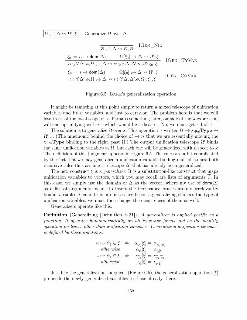
Ω → ∆ Ω′; ξ Generalize Ω over ∆.

∅ → ∆ ∅;∅IGen_Nil

ξ0 = α 7→ dom(∆) Ω[ξ0] → ∆ Ω′; ξ

α :ρ ∀∆′.κ,Ω → ∆ α :ρ ∀∆,∆′.κ,Ω′; ξ0, ξIGen_TyVar

ξ0 = ι 7→ dom(∆) Ω[ξ0] → ∆ Ω′; ξ

ι : ∀∆′.φ,Ω → ∆ ι : ∀∆,∆′.φ,Ω′; ξ0, ξIGen_CoVar

Figure 6.5: Bake’s generalization operation

It might be tempting at this point simply to return a mixed telescope of unificationvariables and Pico variables, and just to carry on. The problem here is that we willlose track of the local scope of x . Perhaps something later, outside of the λ-expression,will end up unifying with x—which would be a disaster. No, we must get rid of it.

The solution is to generalize Ω over x . This operation is written Ω → x :RelType Ω′; ξ. (The mnemonic behind the choice of → is that we are essentially moving thex :RelType binding to the right, past Ω.) The output unification telescope Ω′ bindsthe same unification variables as Ω, but each one will be generalized with respect to x .The definition of this judgment appears in Figure 6.5. The rules are a bit complicatedby the fact that we may generalize a unification variable binding multiple times; bothrecursive rules thus assume a telescope ∆′ that has already been generalized.

The new construct ξ is a generalizer. It is a substitution-like construct that mapsunification variables to vectors, which you may recall are lists of arguments ψ. Inthis case, we simply use the domain of ∆ as the vector, where my use of dom(∆)as a list of arguments means to insert the irrelevance braces around irrelevantlybound variables. Generalizers are necessary because generalizing changes the type ofunification variables; we must then change the occurrences of them as well.

Generalizers operate like this:

Definition (Generalizing [Definition E.31]). A generalizer is applied postfix as afunction. It operates homomorphically on all recursive forms and as the identityoperation on leaves other than unification variables. Generalizing unification variablesis defined by these equations:

α 7→ ψ1 ∈ ξ ⇒ αψ2[ξ] = αψ1,ψ2

otherwise αψ[ξ] = αψ[ξ]

ι 7→ ψ1 ∈ ξ ⇒ ιψ2[ξ] = ιψ1,ψ2

otherwise ιψ[ξ] = ιψ[ξ]

Just like the generalization judgment (Figure 6.5), the generalization operation [ξ]prepends the newly generalized variables to those already there.

159

Σ; Ψ ty t τ : κ a Ω synthesize a type (no invis. binders)Σ; Ψ ∗

ty t τ : κ a Ω synthesize a typeΣ; Ψ ty t : κ τ a Ω check a type (no invis. binders)Σ; Ψ ∗

ty t : κ τ a Ω check a typeΣ; Ψ pt s τ a Ω check a polytype (always with kind Type)

Σ; Ψ; ρ ∗arg t : κ ψ; τ a Ω check an argument at relevance ρΣ; Ψ;κ0; τ0 alt alt : κ alt a Ω check a case alt. against an unknown typeΣ; Ψ;κ0; τ0 altc alt : κ alt a Ω check a case alt. against a known type

Σ; Ψ q qvar a : κ; ν a Ω synth. type of a bound var.Σ; Ψ aq aqvar a : κ a Ω synth. type of a bound var. (w/o vis. marker)

Σ; Ψ aq aqvar : κ a : κ′; x .τ a Ω check type of a bound var. (w/o vis. marker)pi quant Π; ρ interpret a quantifier

fun κ; ρ1 γ; Π; a; ρ2;κ1;κ2 a Ω extract components of a function typeΣ; Ψ scrut alt;κ γ; ∆;H ; τ a Ω extract components of a scrutinee type

νinst κ ψ;κ′ a Ω instantiate a type

Σ; Γ decl decl x : κ := τ check a declarationΣ; Γ prog prog Γ′; θ check a program

Figure 6.6: Bake judgments

6.6 Type inference algorithmThe schema of the judgments that define Bake appear in Figure 6.6. I will not walkthrough each rule of each judgment to explain its inner workings. As discussed inthe introduction to this chapter, the individual rules are largely predictable. Theycan be reviewed in their entirety in Appendix D, and the statements of lemmas thatassert the soundness of many of these judgments appear in Section 6.8.1.4. Insteadof a thorough review of the algorithm, this section will call out individual rules withinteresting characteristics.

6.6.1 Function application

As discussed above (Section 6.4) function applications can only synthesize their type.The two rules for synthesizing the type of a function application (one for regularapplication and one for application with @) appear in Figure 6.7 on the next page,along with auxiliary judgments.

Walking through the ITy_App rule, we see that Bake first infers the type κ0

for the Haskell expression t1, elaborating t1 to become τ1 and producing a unificationtelescope Ω1. The type for τ1, though, might not manifestly be a function. This wouldhappen, for example, when inferring the type of λx y → x y , where the type initiallyassigned to x is just a unification variable α. Instead of writing κ0 as a function, Bake

160

Σ; Ψ ty t1 τ1 : κ0 a Ω1

fun κ0; Rel γ; Π; a; ρ;κ1;κ2 a Ω2

Σ; Ψ,Ω1,Ω2; ρ ∗arg t2 : κ1 ψ2; τ2 a Ω3

Σ; Ψ ∗ty t1 t2 (τ1 B γ)ψ2 : κ2[τ2/a] a Ω1,Ω2,Ω3

ITy_App

Σ; Ψ ∗ty t1 τ1 : ΠSpeca:ρκ1. κ2 a Ω1

Σ; Ψ,Ω1; ρ ∗arg t2 : κ1 ψ2; τ2 a Ω2

Σ; Ψ ∗ty t1 @t2 τ1 ψ2 : κ2[τ2/a] a Ω1,Ω2

ITy_AppSpec

fun κ; ρ1 γ; Π; a; ρ2;κ1;κ2 a Ω Extract out the parts of a function kind.

fun ΠReqa:ρκ1. κ2; ρ0 〈ΠReqa:ρκ1. κ2〉; Π; a; ρ;κ1;κ2 a ∅IFun_Id

fresh ι fresh β1, β2

Ω = β1:IrrelType, β2:IrrelType, ι:κ0 ∼˜ΠReqa:ρβ1. β2

fun κ0; ρ ι;˜Π; a; ρ; β1; β2 a Ω

IFun_Cast

Σ; Ψ; ρ ∗arg t : κ ψ; τ a Ω Check a function argument against its known type.

Σ; Ψ ∗ty t : κ τ a Ω

Σ; Ψ; Rel ∗arg t : κ τ ; τ a ΩIArg_Rel

Σ; Rel(Ψ) ∗ty t : κ τ a Ω

Σ; Ψ; Irrel ∗arg t : κ τ; τ a ΩIArg_Irrel

Figure 6.7: Function applications in Bake

instead uses its fun judgment, which extracts out the component parts of a functiontype.

It may be helpful in understanding the fun judgment to see its correctness property,as proved in Section E.9:

Lemma (Function position [Lemma E.37]). If Σ; Ψ ty κ : Type and fun κ; ρ1 γ; Π; a; ρ2;κ1;κ2 a Ω, then Σ; Ψ,Ω co γ : κ ∼ ΠReqa:ρ2κ1. κ2.

We can see here that fun produces a coercion γ that relates the input type κ tothe output type Πa:ρ2κ1. κ2. The input relevance ρ1 is to be used as a default—Bakewill assume that a function uses its argument relevantly unless told otherwise. Notethat relevance of arguments is not denoted in the user-written source code.

Looking at the definition of fun, we see two cases:

• If the input type κ is manifestly a Π-type, Bake just returns its componentpieces along with a reflexive coercion.

161

• Otherwise, it invents fresh unification variables as emits a constraint relatingthis variables to the input.

It might be tempting to define fun only by the second rule, IFun_Cast, but thiswould greatly weaken Bake’s power. Doing so would mean that the bidirectionalalgorithm would never be able to take advantage of knowing a function’s argumenttype. Furthermore, note that β2, the result type of the function in IFun_Cast, is notgeneralized with respect to a:ρβ1; a function type inferred via IFun_Cast will surelybe non-dependent. This decision was made in keeping with the guiding principle thatonly simple types should be inferred.

Once we have extracted the component parts of the function type, we can check theargument with the ∗arg judgment. This judgment takes the relevance of the argumentas an input; it simply uses the ∗ty checking judgment and insert braces as appropriate.

Contrast the behavior of ITy_App to that of ITy_AppSpec, which, crucially,does not use fun. Consider what would happen if the function’s type is not manifestlya Π-type. We could, like in IFun_Cast invent unification variables and emit aconstraint. But this would mean that the argument is inferred, not specified. Using aninferred argument with a visibility override violates the inference principles set forthby Eisenberg et al. [33] and would surely eliminate the possibility of principal types.Accordingly, ITy_AppSpec avoids such behavior and simply looks to make sure thatthe function’s type is of the appropriate shape. If it is not, Bake issues an error.

6.6.2 Mediating between checking and synthesis

The two modes of Bake meet head-on when we are checking an expression (such as afunction application) that has no rules in the checking judgment. The fall-throughcase of the checking judgment is this rule:

Σ; Ψ ∗ty t τ : κ1 a Ω

pre κ2 ∆;κ′2; τ2

Ω → ∆ Ω′; ξ1

κ1[ξ1] ≤∗ κ′2 τ ′2 a Ω2

Ω2 → ∆ Ω′2; ξ2

Σ; Ψ ty t : κ2 τ2 (λ∆. τ ′2[ξ2] τ [ξ1]) a Ω′,Ω′2ITyC_Infer

We are checking that t has type κ2. First, Bake synthesizes t’s type κ1, producingunification telescope Ω. We then must, as described in Section 6.4.3, deeply skolemizeκ2. Pulling out the quantifiers in κ2 (according to the pre judgment) gives us

˜Π∆. κ′2.

We then generalize Ω by ∆. It is this generalization step that allows the solver to solveunification variables in Ω with skolems in ∆ and allows the example from Section6.4.3 to be accepted. Having generalized, we then do the subsumption check. We nowmust generalize Ω2, the output unification telescope from the subsumption check, asΩ2 might refer to skolems bound in ∆.

162

Once again, the key interesting part of this rule is the first generalization step. Itis not necessary to do this in order to get correct elaboration, but the analysis in myprior work [33, end of Section 6.1] suggests that this is necessary in order to haveprincipal types.

6.6.3 case expressions

We see in Figure 6.6 on page 160 that there are two judgments for checking casealternatives. These correspond to the two rules for checking case expressions, one forsynthesis (ITy_Case) and one for checking (ITyC_Case). I refrain from includingthe actual rules here, as their myriad and ornate details would be distracting; theoverly curious can see Appendix D for these details.

As discussed previously (Sections 4.3.3 and 6.4), a case expression is treateddifferently depending on whether we can know its result type. In the case wherewe do not (ITy_Case), Bake invents a new unification variable β for the resulttype and checks each case alternative against it. This is why the alt judgment takesa result type, even though it is used during synthesis. After all, we do require allalternatives to produce the same result type. Producing the unification variable withineach alternative would risk running into a skolem escape, whereby the result typemight mention a variable locally bound within the alternative. It is simpler just topropagate the β down into alt. The alt judgment, in turn, does not use the equalitygotten from dependent pattern matching when checking alternatives. Recall that doingso during synthesis mode would cause trouble because the equality assumption wouldmake the β unification variable untouchable when solving constraints emitted whileprocessing the alternatives.

On the other hand, the altc judgment is used from ITyC_Case, in checking mode.This judgment is almost identical to alt except that it allows the alternatives to makeuse of the dependent-pattern-match equality.

6.6.4 Checking λ-expressions

Consider checking this expression:

(λ(f :: Int → Int)→ f 5) :: (∀ a. a→ a)→ Int (6.6.1)

This expression should be accepted. The λ takes a function over Ints and appliesit. The type signature then says that the λ should actually be applicable to anypolymorphic endofunction. Of course, such a function can be specialized to Int, so allis well. Indeed, the expression above is accepted by GHC.

The example above, however, is not dependent. Surprisingly, the intuition in theabove paragraph does not generalize to the dependent case. Consider this (contrived)

163

example:

(λ(f :: Bool → Bool)→ P) :: Π (g :: ∀ a. a→ a)→ Proxy ’(g 5, g ’True) (6.6.2)

where we have

data Proxy :: ∀ k . k → Type whereP :: ∀ k (a :: k). Proxy a-- equivalent to data Proxy a = P

Once again, the annotation on the λ argument is a specialized version of the argument’stype as given in the type signature. And yet, this expression must be rejected.

One way to boil this problem down is to consider what type we check the expressionP against. When we are checking P , we clearly have f :: Bool → Bool in scope. Yetthe natural type to check P against is Proxy ’(g 5, g ’True), which mentions g , notf . Even if the names were to be fixed, we would still have the problem that g 5 iscertainly not well typed if g has type Bool → Bool . We are stuck.

Another way to see this problem is to think about elaborating the subsumptionjudgment. In example (6.6.1), type inference will check whether ∀ a. a→ a ≤ Int → Int.When it discovers that this is true, the subsumption algorithm will also produce afunction that takes something of type ∀ a. a→ a to something of type Int → Int. If theexpression in example (6.6.1) is applied to an argument (naturally, of type ∀ a. a→ a),then this conversion function readies the argument to pass to the λ-expression.

In example (6.6.2), however, we need conversions both ways. We still need theconversion from ∀ a. a→ a to Bool → Bool , for exactly the same reason that we needit for example (6.6.1). We also need the conversion in the other direction (in this case,the impossible conversion from Bool → Bool to ∀ a. a → a) when checking that P ,with f :: Bool → Bool in scope, has type Proxy ’(g 5, g ’True), using g :: ∀ a. a→ a.

The solution to this is to have two separate rules, one in the non-dependent caseand one in the dependent case. Bake looks at the type being checked against (let’scall it τ). If τ uses its argument dependently, then Bake requires that the annotationon the λ argument and the function type as found in τ can be proved equal—thatis, that there is a coercion between them. Otherwise, we use subsumption, just as inexample (6.6.1). You can view the two rules in Section D.5; as usual, the rules are abit cluttered to present here.

6.7 Program elaborationUp until now, this chapter has focused more on the gate-keeping services provided byBake, preventing ill formed programs from being accepted. In this section, we willdiscuss elaboration, the process of creating the Pico program that corresponds to aninput Haskell program. Let’s look in particular on the highest levels of elaboration,processing Haskell declarations and programs. See Figure 6.8 on the next page for thetwo judgments of interest.

164

Σ; Γ decl decl x : κ := τ Check a Haskell declaration.

Σ; Γ ty t τ : κ a ΩΣ; Γ solv Ω ∆; Θτ ′ = λ∆. (τ [Θ]) κ′ =

˜ΠInf∆. (κ[Θ])

Σ; Γ decl x := t x : κ′ := τ ′IDecl_Synthesize

Σ; Γ pt s σ a Ω1

Σ; Rel(Γ) solv Rel(Ω1) ∆1; Θ1

σ′ =˜ΠInf∆1. (σ[Θ1])

Σ; Γ ∗ty t : σ′ τ a Ω2

Σ; Γ solv Ω2 ∅; Θ2

τ ′ = τ [Θ2]

Σ; Γ decl x :: s := t x : σ′ := τ ′IDecl_Check

Σ; Γ prog prog Γ′; θ Check a Haskell program.

Σ; Γ prog ∅ ∅;∅IProg_Nil

Σ; Γ decl decl x : κ := τΣ; Γ, x :Relκ, c:x ∼ τ prog prog Γ′; θ

Σ; Γ prog decl; prog x :Relκ, c:x ∼ τ,Γ′; (τ/x , 〈τ〉/c) θIProg_Decl

Figure 6.8: Elaborating declarations and programs

6.7.1 Declarations

The decl judgment processes the two forms of declaration included in the Haskellsubset formalized here: unannotated variable declarations and annotated variabledeclarations. It outputs the name of the new variable, its type κ and its value τ .Note that the environment used in decl is Σ; Γ, with a context containing only Picovariables, no unification variables. These are top-level declarations only.

Rule IDecl_Synthesize simply ties together the pieces of using the synthesisjudgment and the solver. Note that the definitions of τ ′ and κ′ in the rule generalizeover the telescope ∆ produced by the solver, and that the Π-type formed marks thebinders as inferred, never specified.

Rule IDecl_Check is a bit more involved. It first must check the type signatureusing the pt judgment, to make sure s it is a well formed polytype. This process mightemit constraints, and we must solve these before tackling the term-level expression.This would happen, for example, in the type ∀ a. Proxy a → (), as a’s kind isunspecified. The solver may produce a telescope ∆1 to generalize by. In our example,this telescope would include k :IrrelType, the type of a. Having sorted out the type

165

signature, we can now proceed to the expression t, which is checked against σ′ thegeneralized Pico translation of the user-written polytype s. We must solve once again.In this invocation of the solver, we insist that no further generalization be done becausethe user has already written the entire type of the expression. This decision is inkeeping with standard Haskell, where a declaration like

bad :: a→ Stringbad x = show x

is rejected, because accepting the function body requires generalizing over an extraShow a constraint.

6.7.2 Programs

The elaboration of whole programs is generally straightforward. This algorithm appearsin Figure 6.8 on the preceding page. The judgment Σ; Γ prog prog Γ′; θ produces asoutput an extension to the context, Γ′, as well as a closing substitution θ which mapsthe newly bound variable to its definition. (Recall that this formalization of Bakeignores recursion; thus no variable can be mentioned in its own declaration.)

The one non-trivial rule, IProg_Decl, checks a declaration and then incorporatesthis declaration into the context Γ used to check later declarations. There is one smalltwist here, though: because declared variables can be used in types as well as in terms,we wish the typing context to remember the equality between the variable and itsdefinition. This is done via the coercion variable c included in the context in thesecond premise to IProg_Decl.

6.8 MetatheoryThis chapter has explained the Bake algorithm in some detail, but what theoreticalproperties does it have? A type inference algorithm is often checked for soundnessand completeness against a specification. However, as argued by Vytiniotis et al. [99,Section 6.3], lining up an algorithm such as Bake against a declarative specificationis a challenge. Instead of writing a separate, non-algorithmic form of Bake, I presentthree results in this section:

• I prove that the elaborated Pico program produced by Bake is indeed a welltyped Pico program. This result—which I call soundness—marks an upper limiton the set of programs that Bake accepts. If it cannot be typed in Pico, Bakemust reject.93

93I do not prove a correspondence between the Haskell program and the Pico program producedby elaboration. It would thus theoretically be possible to design Bake to accept all input texts andproduce a trivial elaborated program. But that wouldn’t be nearly as much fun, and I have not doneso.

166

• In two separate subsections, I argue that Bake is a conservative extensionboth of the OutsideIn algorithm and the SB algorithm of Eisenberg et al. [33].That is, if OutsideIn or SB accepts a program, so does Bake. This resultssuggests that a version of GHC based on Bake will accept all Haskell programscurrently accepted. These arguments—I dare not quite call them proofs—arestated in less formal terms than other proofs in this dissertation. While it is likelypossible to work out the details fully, the presentation of the other systems andof Bake/Pico differ enough that the translation between the systems wouldbe fiddly, and artifacts of the translation would obscure the main point. Theindividual differences are discussed below.

These conservativity results provide a lower bound on the power of Bake,declaring that some set of Haskell programs must be accepted by the algorithm.

The results listed above bound the power of the algorithm both from below andfrom above, serving roughly as soundness and completeness results. It is left as futurework to define a precise specification of Bake and prove that it meets the specification.

6.8.1 Soundness

Here is the fundamental soundness result:

Theorem (Soundness of Bake elaboration [Theorem E.44]). If Σ ctx Γ ok andΣ; Γ prog prog Γ′; θ, then:

1. Σ ctx Γ,Γ′ ok

2. Σ; Γ subst θ : Γ′

3. dom(prog) ⊆ dom(Γ′)

This theorem assumes that the starting environment is well formed Σ ctx Γ ok andthat Bake accepts the source language program prog. In return, the theorem claimsthat the context extension Γ′ is well formed (assuming it is appended after Γ), thatthe substitution θ is a valid closing substitution (see below), and that indeed the newcontext Γ′ binds the variables declared in prog.

Closing substitutions are recognized by the new judgment subst, which appears inFigure 6.9 on the next page. (Note the turnstile `; this is a pure Pico judgment withno unification variables in sight.) It uses a new notation θ|z which restricts the domainof a substitution θ to operate only on the variables z . Informally, Σ; Γ subst θ : ∆ holdswhen the substitution θ eliminates the appearance of any of the variables in ∆. Hereis the key lemma that asserts the correctness of the judgment:

Lemma (Closing substitution [Lemma E.30]). If Σ; Γ subst θ : ∆ and Σ; Γ,∆,Γ′ ` J ,then Σ; Γ,Γ′[θ|dom(∆)] ` J [θ|dom(∆)].

167

Σ; Γ subst θ : ∆ “θ substitutes the variables in ∆ away.”

Σ; Γ subst θ : ∅Subst_Nil

Σ; Γ ty a[θ] : κΣ; Γ subst θ : ∆[θ|a ]

Σ; Γ subst θ : a:Relκ,∆Subst_TyRel

Σ; Rel(Γ) ty a[θ] : κΣ; Γ subst θ : ∆[θ|a ]

Σ; Γ subst θ : a:Irrelκ,∆Subst_TyIrrel

Σ; Rel(Γ) co c[θ] : φΣ; Γ subst θ : ∆[θ|c]Σ; Γ subst θ : c:φ,∆

Subst_Co

Figure 6.9: Validity of closing substitutions

Here, I use a notation where J stands for a judgment chosen from ty, co, prop, alt,vec, ctx, or s.

The use of subst in the conclusion of the elaboration soundness theorem means thatthe variable values stored in θ actually have the types as given in Γ′.

Naturally, proving this theorem requires proving the soundness of all the individualjudgments that form Bake. These proofs all appear in Section E.9.

6.8.1.1 Adapting lemmas on ` to

The first step in establishing the soundness result is to ensure that the structurallemmas proved for ` judgments still hold over the judgments. While doing thisfor the definitions as given does not pose a challenge, it is in getting these proofs towork that all of the complications around unification variables (to wit, zonkers andgeneralizers) arise.

Relating the two sets of judgments is accomplished by this key lemma:

Lemma (Extension [Lemma E.3]). Σ; Γ ` J if and only if Σ; Γ J .

Note that the context must contain only Pico variables, never unification variables.This fact is what allows the larger Σ; Γ J to imply the smaller Σ; Γ ` J .

168

Σ; Ψ z Θ : Ω “Θ zonks all the unification variables in Ω.”

Σ; Ψ z ∅ : ∅Zonk_Nil

Σ; Ψ,∆ ty τ : κΣ; Ψ z Θ : Ω[∀ dom(∆).τ/α]

Σ; Ψ z ∀ dom(∆).τ/α,Θ : α :Rel ∀∆.κ,ΩZonk_TyVarRel

Σ; Rel(Ψ,∆) ty τ : κΣ; Ψ z Θ : Ω[∀ dom(∆).τ/α]

Σ; Ψ z ∀ dom(∆).τ/α,Θ : α :Irrel ∀∆.κ,ΩZonk_TyVarIrrel

Σ; Ψ,∆ co γ : φΣ; Ψ z Θ : Ω[∀ dom(∆).γ/ι]

Σ; Ψ z ∀ dom(∆).γ/ι,Θ : ι : ∀∆.φ,ΩZonk_CoVar

Figure 6.10: Zonker validity

6.8.1.2 Soundness of the solver

The solver Σ; Ψ solv Ω ∆; Θ produces a generalization telescope and a zonker. Inorder to define a correctness property for this solver, we first need a judgment thatasserts the validity of the zonker. This judgment appears in Figure 6.10. The judgmentis quite similar to the judgment classifying closing substitutions ( subst, in Figure 6.9on the previous page), but it deals also with the complexity of having unificationvariables quantified over telescopes.

Naturally, we must require that the solver produce a valid zonker. We also requirethat the zonker be idempotent, as that is a necessary requirement to prove the zonkinglemma, below. Here is the soundness property we are assuming of the solver. Notethat this property is the only one we need to prove soundness of elaboration.

Property (Solver is sound [Property E.24]). If Σ ctx Ψ,Ω ok and Σ; Ψ solv Ω ∆; Θ,then Θ is idempotent, Σ ctx Ψ,∆ ok, and Σ; Ψ,∆ z Θ : Ω.

Lemma (Zonking [Lemma E.23]). If Θ is idempotent, Σ; Ψ z Θ : Ω, and Σ; Ψ,Ω,∆ J , then Σ; Ψ,∆[Θ] J [Θ].

6.8.1.3 Soundness of generalization

The following lemma asserts the correctness of the generalization judgment:

Lemma (Generalization [Lemma E.35]). If Ω → ∆ Ω′; ξ and Σ; Ψ,∆,Ω J , thenΣ; Ψ,Ω′,∆ J [ξ].

The proof of this lemma relies on the following smaller lemma (and its counterpartfor coercion variables):

169

Lemma (Generalization by type variable [Lemma E.32]). If Σ; Ψ,∆, α :ρ ∀∆′.κ,Ψ′ J , then Σ; Ψ, α :ρ ∀∆,∆′.κ,∆,Ψ′[α 7→ dom(∆)] J [α 7→ dom(∆)].

6.8.1.4 Soundness lemmas for individual judgments

Lemma (Instantiation [Lemma E.36]). If Σ; Ψ ty τ : κ and νinst κ ψ;κ′ a Ω, thenΣ; Ψ,Ω ty τ ψ : κ′ and κ′ is not a Π-type with a binder (with visibility ν2) such thatν2 ≤ ν.Lemma (Scrutinee position [Lemma E.38]). If Σ; Ψ ty τ : κ and Σ; Ψ scrut alt;κ γ; ∆;H ′; τ a Ω, then Σ; Ψ,Ω ty τ B γ : ’Π∆.H ′ τ and Σ; Rel(Ψ,Ω) ty H ′ τ : Type.Lemma (Prenex [Lemma E.40]). If Σ; Rel(Ψ) ty κ : Type and pre κ ∆;κ′; τ , thenΣ; Ψ ty τ :

˜Πx :Rel(

˜Π∆. κ′). κ.

Lemma (Subsumption [Lemma E.41]). Assume Σ; Rel(Ψ) ty κ1 : Type andΣ; Rel(Ψ) ty κ2 : Type. If either

1. κ1 ≤∗ κ2 τ a Ω, or

2. κ1 ≤ κ2 τ a Ω,then Σ; Ψ,Ω ty τ :

˜Πx :Relκ1. κ2.

Lemma (Type elaboration is sound [Lemma E.42]).1. If any of the following:

(a) Σ ctx Ψ ok and Σ; Ψ ty t τ : κ a Ω, or(b) Σ ctx Ψ ok and Σ; Ψ ∗

ty t τ : κ a Ω, or(c) Σ; Rel(Ψ) ty κ : Type and Σ; Ψ ty t : κ τ a Ω, or(d) Σ; Rel(Ψ) ty κ : Type and Σ; Ψ ∗

ty t : κ τ a Ω,

then Σ; Ψ,Ω ty τ : κ.

2. If Σ ctx Ψ ok and Σ; Ψ pt s σ a Ω, then Σ; Rel(Ψ,Ω) ty σ : Type.

3. If Σ; Ψ ty τ1 : Πνa:ρκ1. κ2 and Σ; Ψ; ρ ∗arg t2 : κ1 ψ2; τ2 a Ω, then Σ; Ψ,Ω tyτ1 ψ2 : κ2[τ2/a].

4. If Σ; Rel(Ψ) ty κ : Type, Σ; Ψ ty τ0 : ’Π∆.H τ , Σ; Rel(Ψ) ty H τ : Type, andΣ; Ψ; ’Π∆.H τ ; τ0 alt alt : κ alt a Ω, then Σ; Ψ,Ω; ’Π∆.H τ τ0alt alt : κ.

5. If Σ; Rel(Ψ) ty κ : Type, Σ; Ψ ty τ0 : ’Π∆.H τ , Σ; Rel(Ψ) ty H τ : Type, andΣ; Ψ;κ0; τ0 altc alt : κ alt a Ω, then Σ; Ψ,Ω;κ0

τ0alt alt : κ.

6. If Σ ctx Ψ ok and Σ; Ψ q qvar a : κ; ν a Ω, then Σ; Rel(Ψ,Ω) ty κ : Type.

7. If Σ ctx Ψ ok and Σ; Ψ aq aqvar a : κ a Ω, then Σ; Rel(Ψ,Ω) ty κ : Type.

8. If Σ; Ψ ty τ0 : κ and Σ; Ψ aq aqvar : κ a : κ′; x .τ a Ω, then Σ; Ψ,Ω ty τ [τ0/x ] :κ′.

170

OutsideIn construct Pico form NotesAxiom scheme Q Γ instances, etc.; implications are func-

tions; type family instances are viaunfoldings

Given constraint Qg, Qr ∆ constraints are named in PicoWanted constraint Qw Ω we must separate wanteds & givens

Figure 6.11: Translation from OutsideIn to Pico

6.8.2 Conservativity with respect to OutsideIn

I do not endeavor to give a full accounting of the OutsideIn algorithm here, insteadreferring readers to the original [99]. I will briefly explain judgments, etc., as theyappear and refer readers to Figure numbers from the original text.

There are several mismatches between concepts in OutsideIn and in Pico. Chiefamong these is that OutsideIn does not track unification variables in any detail.All unification variables (and type variables, in general) in OutsideIn have kindType, and thus there is no need for dependency tracking. In effect, many judgments inOutsideIn are parameterized by an unwritten set of in-scope unification variables. Wehave no such luxury of concision available in Bake, and so there must be considerationgiven to tracking the unification variables.

To partly bridge the gap between OutsideIn and Bake, I define encode whichdoes the translation, according to Figure 6.11. encodeing a construct from the leftcolumn results in a member of the syntactic class depicted in the middle column.

OutsideIn differentiates between algorithm-generated constraints C and user-written ones Q; the former contain implication constraints. I do not discern betweenthese classes, considering implication constraints simply as functions. I will use Qmetavariables in place of OutsideIn’s C.94

A further difference between OutsideIn and Bake is that the latter is bidirectional.When OutsideIn knows the type which it wishes to assign to a term, it synthesizesthe term’s type and then emits an equality constraint. In the comparison between thesystems, we will pretend that Bake’s checking judgments do the same.

The fact that I must change my judgments does not imperil the practical impactof the conservativity result—namely, programs that GHC accepts today will still beaccepted tomorrow. GHC already uses bidirectional type-checking and so has alreadyobviated the unidirectional aspect of OutsideIn. However, in order to make a formalcomparisons between that published algorithm, it is helpful to restrict ourselves to aunidirectional viewpoint.

A final difference is that Bake does elaboration, while OutsideIn does not. I94This conflation of Q and C does not mean that Dependent Haskell is now required to implement

implication constraints; it would be easy to add a post-type-checking pass (a “validity” check, in thevocabulary of the GHC implementation) that ensures that no constraints have implications.

171

shall use the symbol · to denote an elaborated type that is inconsequential in thiscomparison.

6.8.2.1 Expressions

Claim (Expressions [Claim E.45]). If Γ oi t : κ Qw under axiom set Q andsignature Σ, then Σ; Γ, encode(Q) ty t · : κ a α:IrrelType, encode(Qw) whereα = fuv(κ) ∪ fuv(Qw).

This claim relates OutsideIn’s Γ oi t : κ Qw judgment (Figures 6 and 13from Vytiniotis et al. [99]) to Bake’s synthesis ty judgment. Note that the outputΩ from Bake’s judgment must include both the wanteds (encode(Qw)) and also anyunification variables required during synthesis (α).

To argue this claim, we examine the different rules that make up OutsideIn’sjudgment, using structural induction. The details appear in Section E.10.

6.8.2.2 The solver

Property (Solver). If Q;Qg;α1 oisolv Qw Qr; Θ where Σ and Γ capture the signature

and typing context for the elements of that judgment, then

Σ; Γ, encode(Q), encode(Qg) solv α1:IrrelType, encode(Qw)

a2:IrrelType, encode(Qr)[a2/α2]; a2/α2,Θ,

where the a2 are fresh replacements for the α2 which are free in Qr or unconstrainedvariables in α1.

This property is a bit more involved than we would hope, but all of the complicationdeals with Bake’s requirement of tracking unification variables more carefully thandoes OutsideIn. Underneath all of the faffing about with unification variables, thekey point here is that Bake’s solver will produce the same residual constraint Qr asOutsideIn’s and the same zonking substitution Θ.

I do not try to argue this property directly, as I do not present the implemen-tation for the solver. However, this property shows a natural generalization of thesolver in an environment that includes dependencies among variables. Indeed, GHC’simplementation of the solver already handles such dependency.

6.8.2.3 Programs

Claim (Bind). If Γ oi t : κ Qw and Q; ε; fuv(κ) ∪ fuv(Qw) oisolv Qw Qr; Θ, then

Σ; Γ, encode(Q) decl x := t x :˜ΠInfa:IrrelType. (

˜ΠInfencode(Qr). κ[Θ])[a/α] := τ for

some τ , where α = fuv(κ[Θ]) ∪ fuv(Qr) and a are fresh replacements for the α.

This claim relates OutsideIn’s Bind rule (Figure 12) to Bake’s IDecl_Syn-thesize rule. It is a consequence of the claim on expressions and the property aboveof the solver.

172

Claim (Conservativity over OutsideIn). If Q; Γ oi prog, prog contains no annotatedbindings, and Σ captures the signature of the environment prog is checked in, thenΣ; Γ, encode(Q) prog prog Γ′; θ.

This claim relates the overall action of the OutsideIn algorithm (Figure 12) toBake’s algorithm for checking programs. It follows directly from the previous claim.

Because of this, I believe that any program without top-level annotations acceptedby OutsideIn is also accepted by Bake.

6.8.3 Conservativity with respect to System SB

Here, I compare Bake with the bidirectional algorithm (called SB) in Figure 8 ofEisenberg et al. [33]. That algorithm is proven to be a conservative extension bothof Hindley-Milner inference and also of the bidirectional algorithm presented byPeyton Jones et al. [74]. This SB algorithm, along with OutsideIn, is part of thebasis for the algorithm currently implemented in GHC 8.

Before we can successfully relate these systems, we must tweak both a bit to bringtheir approaches more in line with one another:

• System SB assumes an ability to guess monotypes. This is evident, for example,in the SB_Abs rule, where an unannotated λ-expression is processed and themonotype of the argument is guessed. Bake, of course, uses unification variables.I thus modify System SB to always guess a unification variable when it guesses.The modified rules are SB_Abs, SB_InstS, and SB_Var.

• Because of the previous change, it is now unfair in rule SB_App to insist thatthe result of synthesis be a function type. Instead, the result of synthesizing thetype of e1 is an arbitrary monotype, and the fun judgment is used to expand thisout to a proper function type. Note that we do not make a similar change inSB_TApp; doing so would be tantamount to saying that a unification variablemight unify with a type with an invisible binder, something we have forbidden.(See Section 6.10.1.3.) We similarly must modify SB_DAbs to allow for thepossibility of a unification variable being checked against.

• There is no convenient equivalent of integers in Bake; I omit the rule SB_Int.

• Bake does not do let-generalization. I thus modify SB_Let and SB_DLetto use the ∗

sb judgment instead of the generalizing judgment.

• System SB skolemizes deeply in its checking ∗sb judgment, while Bake skolemizesonly shallowly. We thus move the prenex operation from SB_DeepSkol toSB_Infer. I claim that this change does not alter the set of programs thatSystem SB accepts, due to the fact that neither non-Infer rule in the sb

judgment interacts with ∀s.

173

• Bake expends a great deal of effort tracking telescopes of unification variables,requiring the notion of a generalizer ξ. However, in the language supported bySystem SB, all type variables always have kind Type and so these telescopes areunnecessary. We thus simply ignore generalizers and the generalization judgment(which always succeeds, regardless).

The theorem below also needs to relate a context Ψ used in Bake with the moretraditional context Γ used in System SB. In the claim below, I use Ψ ≈ Γ to mean thatall Ψ has no coercion bindings, that all irrelevant bindings in Ψ are of kind Type, andthat no relevant bindings depend on any other. Furthermore, all unification variablesbound in Ψ are absent from Γ.

I can now make the following claim:

Claim (Conservativity with respect to System SB [Claim E.47]). Assume Ψ ≈ Γ.

1. If Γ sb t⇒ κ, then Σ; Ψ ty t · : κ a Ω.

2. If Γ ∗sb t⇒ κ, then Σ; Ψ ∗

ty t · : κ a Ω.

3. If Γ sb t⇐ κ, then Σ; Ψ ty t : κ · a Ω.

4. If Γ ∗sb t⇐ κ, then Σ; Ψ ∗

ty t : κ · a Ω.

A detailed argument for this claim appears in Section E.11.

6.9 PracticalitiesI have designed Bake with an eye toward implementing this algorithm directly inGHC. This section discusses some of the practical opportunities and challenges inintegrating Bake with the rest of GHC/Haskell.

6.9.1 Class constraints

In both Pico and Bake, I conspicuously ignore the possibility of Haskell’s type classesand instances. However, this is because classes and instances are already subsumed bythese formalizations’ handling of regular variables.

Classes in Haskell are already compiled into record types that store the imple-mentations of methods, and instances are record values (often called dictionaries)(Section 2.1). As Pico supports datatypes, it also supports classes. Nothing aboutthe type class system should matter at all in Pico. Indeed, System FC as currentlyimplemented in does not GHC 8 cares about type classes, to no ill effect.

During type inference, on the other hand, we need to care a bit about classes andinstances, because these are values that the type inference mechanism fills in for us.However, with Bake’s ability to distinguish visible arguments from invisible ones and

174

its orthogonal ability to work with variables of different relevances, the answer is rightin front of us: an instance is simply an inferred, relevant argument. That’s it! Theseare handled in the following rule, part of the judgment that converts a user-writtenpolytype into Pico:

Σ; Ψ ty t : Type τ a Ω1

Σ; Ψ,Ω1, $a:Relτ pt s σ a Ω2

Ω2 → $a:Relτ Ω′2; ξ

Σ; Ψ pt t⇒ s ˜ΠInf$a:Relτ. (σ[ξ]) a Ω1,Ω′2

IPtC_Constrained

This rule checks the constraint t, making sure it is well typed as a constraint (seeSection 6.9.5) and then checks the rest of the type, assuming the constraint. The useof a $ sign in the name of the constraint ($a) is meant to convey that the variable $acannot appear in the Haskell source.

Note that “given” class constraints (that is, a user-written context on a functiontype signature) are also handled without any effort, as a member of a telescope thatunification variables are quantified over.

In contrast to the Bake constraint generation algorithm, the solver must treatinstances separately and have a way of finding instances in the global set. However,this remains out of scope for this dissertation.

6.9.2 Scoped type variables

Scoped type variables in GHC/Haskell have an idiosyncratic set of rules detailingwhen variables are to be brought into scope [72]. Consider the following two examples,where t is an arbitrary term:

example1 = (t :: ∀ a. a→ a)

higherRank :: (∀ a. a→ a)→ ()example2 = higherRank t

In example1, the type variable a is in scope in t. In example2, however, a is not inscope. This is true despite the fact that, in both cases, Bake would check t againstthe same Pico type.

Instead of trying to track all of this in the constraint generation algorithm, however,Bake divides its pool of variable names into those names that can appear in a sourceprogram (a, b, x ) and those that cannot ($a, $b, $x ). When Bake must put a variable inthe context that should not be available in Haskell, it uses the $a variant. Scoped typevariables are explicitly brought into scope by λ or Λ. It is thus up to the preprocessorwhich must introduce abstractions as necessary to bring the scoped type variablesinto scope; as this process is not type-directed, incorporated this into the preprocessorshould not be a challenge.

175

Bake judgment GHC functionfun matchExpectedFunTysscrut matchExpectedTyConAppinst topInstantiatepre tcDeepSplitSigmaTy_maybe≤∗ tcSubTypeDS≤ tcSubTypeprog tcPolyBinds

Figure 6.12: GHC functions that already implement Bake judgments

6.9.3 Correspondence between Bake and GHC

The design of Bake is already quite close to that of GHC’s constraint-generationalgorithm. Figure 6.12 lists correspondences between Bake judgments and functionsalready existent in GHC.

Notably absent from Figure 6.12 are the main judgments such as ty. These areimplemented in GHC via its tcExpr function, which handles both directions of thebidirectional type system at the same time through its use of expected types, amechanism where the synthesis judgment is implemented by checking against a hole—essentially, a unification variable that can unify with a polytype. A full accounting ofGHC’s expected types and holes is out of scope here, but there should be no troubleadapting Bake’s bidirectional algorithm to GHC as previous bidirectional algorithmshave been adapted.

6.9.4 Unification variables in GHC

The GHC implementation takes a very different approach to unification variablesand zonking than does Bake. A GHC unification variable (called a metavariable inthe source code) is a mutable cell. The solver fills in the mutable cells. Though theimplementation details differ a bit, the same is currently true for unification coercionvariables (called coercion holes in GHC)—they are still mutable cells. The zonkingoperation walks through a type (or coercion or expression) and replaces pointers tomutable cells with the cells’ contents. On the other hand, Bake’s treatment of fillingin unification variables requires building up an explicit zonker Θ; in effect, the implicitsubstitution GHC builds in the heap using mutable cells is made explicit in Bake.

Another key difference between GHC and my formalization (and every other) isthat GHC variables track their own kinds. The implementation does track a contextused in looking up user-written variable occurrences, but no context is needed to, say,extract a type’s kind from the type itself. Because of this design, GHC does not needto track unification telescopes, even though GHC 8 already can have arbitrarily longchains of variables that depend on others. Instead, the solver takes (essentially) the

176

set of unification variables to solve for. Dependency checking is done after the fact asa simple pass making sure all variables in kinds are in scope.

A further consequence of GHC’s design is that there is no need for the concept ofgeneralizers ξ as I have described. Unification variable occurrences are not, in fact,applied to vectors. Along with the fact that GHC does not track contexts, it also usesstable names powered by a enumerable collection of Uniques. We thus do not have toworry about arbitrary α-renaming during constraint generation and solving. Takentogether, the need for generalizers is lost, and thus the generalization operation →disappears.

6.9.5 Constraint vs. Type

Haskell includes the kind Constraint that classifies all constraints; we thus haveShow :: Type→ Constraint. However, due to the datatype encoding of classes and thedictionary encoding of instances, Pico manipulates constraints just as it does ordinarytypes. For this reason, Pico makes no distinction between Constraint and Type. Thischoice follows GHC’s current practice, where Constraint and Type are distinct in thesource language but indistinguishable in the intermediate language. This design hassome unfortunate consequences; see GHC ticket #11715 for a considerable amount ofdiscussion.

Extending the language with dependent types is orthogonal to the problemspresented there, however. For simplicity, Bake as described here does not recognizeConstraint, putting all constraints in the kind Type with all the other types.

6.10 Discussion

6.10.1 Further desirable properties of the solver

Thus far, I have stated only one property (in Section 6.8.1.2) that the solver mustmaintain, that it must output a valid zonker. However, it is helpful to describe furtherproperties of the solver in order to make type inference more predictable and tomaintain the properties stated by Vytiniotis et al. [99], such as the fact that allinferred types are principal and that the solver makes no guesses. The full set of extraproperties are listed in Figure 6.13 on the next page.

6.10.1.1 Entailment

These properties are stated with respect to an entailment relation, defined as follows:

Definition (Entailment). We say that an environment Σ; Ψ entails a telescope ∆,written Σ; Ψ ( ∆, if there exists a vector ψ such that Σ; Ψ vec ψ : ∆.

177

Property 6.1 (Solver is guess-free). If Σ; Ψ solv Ω ∆; Θ, then Σ; Ψ,Ω ( ∆, EΘ,where EΘ = _:α ∼ τ | ∀ z .τ/α ∈ Θ is the equational constraint induced by thezonker Θ.

The above property is adapted from Vytiniotis et al. [99, Definition 3.2 (P1)].

Property 6.2 (Solver avoids non-simple types). If Σ; Ψ solv Ω ∆; Θ and ∀ z .τ/α ∈Θ, then τ is a simple type, with no invisible binders (at any level of structure) and nodependency.

Property 6.3 (Solver does not generalize over coercions). If Σ; Ψ solv Ω ∆; Θ,then ∆ binds no coercion variables.

Figure 6.13: Additional solver properties

As this section expands upon the ideas from Vytiniotis et al. [99], it is necessary tocheck whether this definition of entailment satisfies the entailment requirements fromthat work. These requirements are presented in Figure 6.14 on the following page.

All of this properties are easily satisfied, except for property (R8) (both components)which requires congruence. As explored in some depth in Section 5.8.5.3, Pico simplydoes not have this property. However, that same section argues that equality in Picois “almost congruent”, suggesting that the equality relation truly is congruent in theabsence of coercion abstractions. The proof that the OutsideIn algorithm infersprincipal types does require property R8 [99, Theorem 3.2], and so it is possible thatPico’s lack of congruence prevents Bake from inferring principal types. The detailshave yet to be worked out.

6.10.1.2 A guess-free solver

One of the guiding principles I set forth at the beginning of this chapter is that thealgorithm and solver be guess-free. We thus must assert that the solver is guess-free,an important step along the way to the proof of principal types in Vytiniotis et al.[99]. See Property 6.1.

6.10.1.3 Solver does not introduce impredicativity

An important but previously unstated property is that that solver must not set aunification variable to anything but a simple type, one with no invisible binders nordependency. (Such types are sometimes called τ -types, referring to the τ/σ split in thetypical presentation of the Hindley-Milner type system.) In the context of DependentHaskell, impredicativity has perhaps an unusual definition: no type variable is everinstantiated with a non-simple type. For this to hold, however, we must make surethat this property extends to unification variables as well, as those are sometimes usedto instantiate regular variables.

178

Reflexivity Σ; Ψ,∆ ( ∆ (R1)Transitivity Σ; Ψ,∆1 ( ∆2 ∧ Σ; Ψ,∆2 ( ∆3 =⇒ Σ; Ψ,∆1 ( ∆3 (R2)Substitution Σ; Ψ,∆1,Ψ

′ ( ∆2 ∧ Σ; Ψ subst θ : ∆1 (R3)=⇒ Σ; Ψ,Ψ′[θ] ( ∆2[θ]

Type eq. reflexivity Σ; Ψ ty τ : κ =⇒ Σ; Ψ ( _:τ ∼ τ (R4)Type eq. symmetry Σ; Ψ ( _:τ1 ∼ τ2 =⇒ Σ; Ψ ( _:τ2 ∼ τ1 (R5)Type eq. transitivity Σ; Ψ ( _:τ1 ∼ τ2 ∧ Σ; Ψ ( _:τ2 ∼ τ3 (R6)

=⇒ Σ; Ψ ( _:τ1 ∼ τ3

Conjunctions Σ; Ψ ( ∆1 ∧ Σ; Ψ ( ∆2 =⇒ Σ; Ψ ( ∆1,∆2 (R7)Substitutivity Σ; Ψ ( _:τ1 ∼ τ2 ∧ Σ; Ψ, a:Relκ0 ty τ : κ (R8a)

=⇒ Σ; Ψ ( _:τ [τ1/a] ∼ τ [τ2/a]Σ; Rel(Ψ) ( _:τ1 ∼ τ2 ∧ Σ; Ψ, a:Irrelκ0 ty τ : κ (R8b)

=⇒ Σ; Ψ ( _:τ [τ1/a] ∼ τ [τ2/a]

Figure 6.14: Required properties of entailment, following [99, Figure 3]

Solving unification variables with simple types is also important in the contextof the theory around principal types developed in my prior work [33]. Specifically,we must ensure that there are no invisible binders that are hidden underneath aunification variable. By forbidding filling a unification variable with a non-simple type,we have achieved this goal. See Property 6.2.

6.10.2 No coercion abstractions

In stating that Pico supports type erasure (Section 5.11), I admit that type erasuredoes not mean that we can erase coercion abstractions or applications, even thoughwe can erase the coercions themselves. Nevertheless, I argue that Pico can claim tosupport full type erasure because Bake never produces a Pico program that evaluatesto a coercion abstraction. To support this claim, we can look at the elaborated programproduced by Bake and where coercion abstractions can be inserted:

Around subsumption: Three rules extract out a telescope of binders using the prejudgment and then use these binders in the elaboration. If the telescope includesa coercion binder, the elaboration will include a coercion abstraction. However,I am arguing that there should be no coercion binders there in the first place, sowe can handle this case essentially by induction. (Rules affected: ITyC_Infer,rules in the pre judgment, and ISub_DeepSkol)

During generalization after running the solver: If the solver produces a tele-scope that binds coercions, Bake will similarly include a coercion abstract in itselaboration. We must thus assert Property 6.3. This property is not as restrictive

179

as it may seem, as the solver may still abstract over a class constraint whoseinstances store a coercion.95 (Rule affected: IDecl_Synthesize)

Elaborating case alternatives: When elaborating a case alternative, coercion ab-stractions are inserted. This is necessary for two reasons:

• GADT equalities can be brought into scope in a case alternative. Theseare bound by coercion abstractions.

• The dependent-pattern-match equality (Section 4.3.3) must be broughtinto scope by a coercion abstraction.

However, when a case expression is evaluated (by evaluation rule S_Match),these coercion abstractions will be applied to arguments and thus cannot be thefinal value of evaluating the outer Pico expression. (Rules affected: IAlt_Con,IAltC_Con)

These are the only Bake rules that can include a coercion abstraction in theirelaborated types. I thus conclude that type erasure is valid, with no possibility ofhaving evaluation be stuck on a coercion abstraction.

6.10.3 Comparison to Gundry [37]

The Bake algorithm presented here is very similar to the type inference algorithmpresented by Gundry [37, Chapter 7]. Here I review some of the salient differences.

• Gundry includes both a non-deterministic elaboration process and a deterministicone, proving that the deterministic process is sound with respect to the non-deterministic process (at least, in the absence of case). I have omitted a non-deterministic version of the algorithm, instead using the soundness of the resultantPico program to set an upper limit on the programs that Bake can accept.

• Gundry’s inch source language and his evidence intermediate language havetwo forms of case statement: one for traditional, non-dependent pattern match-ing; and one for dependent pattern matching. Bake chooses between thesepossibilities using the difference between checking and synthesis modes.

• While Gundry uses two separate judgments in synthesis mode, he uses only onechecking judgment. The need for two checking judgments here is an innovationthat derives from the need for principal types, as explored in my prior work [33].

• The inch language does not allow annotations on the binders of a λ-abstractionand so Gundry did not encounter the thorny case detailed in Section 6.6.4.

95For example, the Haskell equality constraint ∼ is such a class, distinct from the primitive equalityoperator in Pico. In the terminology of Vytiniotis et al. [100], the Haskell equality is lifted while thePico equality is unlifted.

180

• Gundry’s approach to delayed instantiation for function arguments followsalong the lines of Dunfield and Krishnaswami [24], using an auxiliary judgmentto control function application. While Bake has its ∗arg judgment, which issuperficially similar, Bake’s judgment can only handle one argument at a time.

• Gundry’s algorithm does not do deep skolemization. It would thus not bebackward compatible with GHC’s current treatment of higher-rank types.

• Gundry gives more details about the solver in his algorithm [37, Section 7.5.1].However, this solver is a novel algorithm that remains to be implemented. Instead,Bake targets the OutsideIn solver. Nevertheless, I do not think it would behard for Gundry’s general approach to target OutsideIn, as well.

• As a point of similarity, Gundry’s and Bake’s treatment of unification variablesare very closely aligned. This is not actually intentional—after reading Gundry’sapproach, I believed I could make the whole treatment of unification variablesmuch simpler. Yet despite a variety of attempts, I was unable to make thebasic lemmas that hold together a type system (e.g., substitution, regularity) gothrough without something as ornate as we have both used. I would love to seea simpler treatment in the future, but I do not hold out much hope.

6.11 ConclusionThis chapter has presented Bake, a type checking / inference / elaboration algorithmthat converts type-correct Dependent Haskell types and expressions into Pico. It isproven to produce type-correct Pico code, and it is designed in the hope of supportingprincipal types. Formulating a statement and proof of principal types in Bake isimportant future work.

This algorithm is also designed to work well with GHC’s existing type checkerinfrastructure, and in particular, its constraint solver. It is my hope and plan toimplement this algorithm, quite closely to how it is stated here, in GHC in the nearfuture.

181

Chapter 7

Implementation

This chapter reviews a number of practical issues that arise in the course of imple-menting the theory presented in this dissertation. Perhaps the most interesting ofthese is that the function that computes equality in GHC does not simply check forα-equivalence; see Section 7.2.

7.1 Current state of implementationAs of this writing (August 2016), only a portion of the improvements to Haskelldescribed in this dissertation are implemented. This section describes the current stateof play and future plans.

7.1.1 Implemented in GHC 8

The language supported by GHC 8 is already a large step toward the languagein this dissertation. The features beyond those available in GHC 7 are enabled byGHC’s TypeInType extension. I personally implemented essentially all aspects of thisextension and merged my work in with the development stream. I have had feedbackand bug reports from many users,96 indicating that my new features are alreadygaining traction in the community. Here are its features, in summary:

• The core language is very closely as described in my prior work [105].

• The kind of types ? is now treated as described in Section 7.4.

• Types and kinds are indistinguishable and fully interchangeable.

• Kind variables may be explicitly quantified:

96According to the GHC bug tracker, 19 users (excluding myself) have posted bugs against myimplementation.

182

data Proxy :: ∀ k . k → Type whereProxy :: ∀ k (a :: k). Proxy a

• The same variable can be used in a type and in a kind:

data T whereMkT :: ∀ k (a :: k). k → Proxy a→ T

• Type families can be used in kinds.

• Kind-indexed GADTs:

data G :: ∀ k . k → Type whereGInt :: G IntGMaybe :: G Maybe

data (:≈:) :: ∀ k1 k2. k1 → k2 → Type whereHRefl :: a :≈: a

• Higher-rank kinds are now possible:

class HTestEquality (f :: ∀ k . k → Type) wherehTestEquality :: ∀ k1 k2 (a :: k1) (b :: k2). f a→ f b → Maybe (a :≈: b)

instance HTestEquality TypeRep where -- from Section 3.2.2hTestEquality = eqT

• GADT data constructors can now be used in types.

• The type inference algorithm used in GHC over types directly corresponds tothose rules in Bake that deal with the constructs that are available in types(that is, missing case, let, and λ). This algorithm in GHC is bidirectional, as isBake.

7.1.2 Implemented in singletons

Alongside my work implementing dependent types in GHC, I have also continuedthe development of my singletons package [29, 30]. This package has some enduringpopularity: it has over 7,000 downloads, 31 separate users reporting bugs, is theprimary subject of several blog posts97 and has even made its way into a textbook onHaskell [81, Chapter 13]. The singletons package uses Template Haskell [83], GHC’s

97Here are a sampling:

183

meta-programming facility, to transform normal term-level declarations into type-levelequivalents.

I use my work in singletons as a proof-of-concept for implementing dependent types.My goal with the dependent types work is to make this package fully obsolete. In themeantime, it is an invaluable playground of ideas both for me and other Haskellerswho do not wish to wait for dependent types proper.

Because of its function as a proof-of-concept, I include here a list of featuressupported by singletons. By their support in the library, we can be confident thatthese features can also be supported in GHC without terrible difficulty. The singletonscurrently supports code using the following features in types:

• All term-level constructs supported by Template Haskell except: view patterns,do, list comprehensions, arithmetic sequences. (Template Haskell does notsupport GHC’s arrow notation.) The library specifically does support case, let(including recursive definitions) and λ-expressions. See my prior work for thedetails [29].

• Unsaturated type families and the distinction between matchable and unmatch-able arrows

• Type classes and instances

• Constrained types

• Pattern guards

• Overloaded numeric literals

• Deriving of Eq, Ord , Bounded , and Enum

• Record syntax, including record updates

• Scoped type variables

The latest major effort at improving singletons targeted GHC 7, though the librarycontinues to work with GHC 8. I am confident more constructs could be supportedwith a thorough update to GHC 8—in particular, do-notation cannot be supported inGHC 7 because it would require a higher-kinded type variable. Such type variablesare fully supported in GHC 8, and so I believe singletons could support do-notation

• https://www.schoolofhaskell.com/user/konn/prove-your-haskell-for-great-safety/dependent-types-in-haskell

• https://ocharles.org.uk/blog/posts/2014-02-25-dependent-types-and-plhaskell.html

• http://lambda.jstolarek.com/2014/09/promoting-functions-to-type-families-in-haskell/

• https://blog.jle.im/entry/practical-dependent-types-in-haskell-1.html

all by different authors—not to mention my own posts.

184

and list/monad comprehensions relatively easily now. However, I wish to spend myimplementation efforts on getting dependent types in Haskell for real instead of fakingit with singletons, and so may not complete these upgrades.

7.1.3 Implementation to be completed

There is still a fair amount of work to be done before the implementation of dependenttypes in Haskell is complete. Here I provide a listing of the major tasks to be completedand my thoughts on each task:

• Implement Pico as written in this dissertation. The biggest change over thecurrent implementation of GHC’s intermediate language is that Pico combinesthe grammar of types and of terms. The current intermediate language alreadysupports, for example, heterogeneous equality and the asymmetric bindingcoercion forms (Section 5.8.5.1). While combining the internal datatypes fortypes and terms will be the furthest reaching change, I think the most challengingchange will be the addition of the many different quantifier forms in Pico (withrelevance markers, visibility markers, and matchability markers).

• Combine the algorithms that infer the types of terms and the kinds of types.Currently, GHC maintains two separate, but similar, algorithms: one that type-checks terms and one that kind-checks types. These would be combined, asprescribed by Bake. I expect this to be a simplification when it is all done,as one algorithm will serve where there is currently two—and both are quitecomplex.

• Interleave type-checking with desugaring. Currently, GHC maintains two separatephases when compiling terms: type-checking ensures that the source expressionis well typed and also produces information necessary for elaboration into itsintermediate language. Afterwards, GHC desugars the type-checked program,translating it to the intermediate language. Desugaring today is done only afterthe whole module is type-checked. However, if some declarations depend onevaluating other declarations (because the latter are used in the former’s types),then desugaring and type-checking will have to be interleaved. I do not expectthis to be a challenge, however, for two reasons:

– Type-checking and desugaring are already interleaved, at least in types.Indeed, the kind checker for types produces a type in the intermediatelanguage today, effectively type-checking and desugaring all at once.

– Type-checking happens by going in order through a sequence of mutuallyrecursive groups. One expression cannot depend on another within the samegroup, and so we can just process each group one at a time, type-checkingand then desugaring.

185

• The source language will have to be changed to accept the new features. To behonest, I am a little worried about this change, as it will require updating theparser. Currently, the parsers for types and expressions are separate, but thistask would require combining them. Will this be possible? I already know of oneconflict: the ’ used in Template Haskell quoting (which made a brief appearancein Section 3.1.3.2) and the ’ used in denoting a namespace change. Both of theseelements of the syntax are pre-existing, and so I will have to find some way ofmerging them.

At this point, I do not foresee realistically beginning these implementation tasksbefore the summer of 2017. If that process goes swimmingly, then perhaps we will seeDependent Haskell released in early 2018. More likely, it will be delayed until 2019.

During the process of writing this dissertation, I worked on merging my implemen-tation of TypeInType into the GHC main development stream. This process was muchharder than I anticipated, taking up two more months than expected, working nearlyfull-time. I am thus leery of over-promising about the rest of the implementationtask embodied in this dissertation. However, my success in emulating so many ofthe features in Dependent Haskell in singletons gives me hope that the worst of theimplementation burden is behind me.

Despite not having fully implemented Dependent Haskell, I still have learned muchby implementing one portion of the overall plan. The rest of this chapter shares thishard-won knowledge.

7.2 Type equalityThe notion of type equality used in the definition of Pico is quite restrictive: it issimple α-equivalence. This equality relation is very hard to work with in practice,because it is not proof-irrelevant. That is, Int . 〈Type〉 6= Int. This is true despite thefact that the ∼ relation is proof-irrelevant.

The proof-relevant nature of = poses a challenge in transforming Pico expressionsinto other well typed Pico expressions. This challenge comes to a head in the unifier(Section 7.3) where, given τ1 and τ2, we must find a substitution θ such that τ1 = τ2.Unification is used, for example, when matching class instances. However, with proof-relevant equality, such a specification is wrong; it would fail to find an instanceC (Maybe a) when we seek an instance for C (Maybe Int . 〈Type〉). Instead, we wantθ and γ such that Σ; Γ co γ : τ1[θ] ∼ τ2[θ] (for an appropriate Σ and Γ). Experiencehas shown that constructing the γ is a real challenge.98

98When I attempted this implementation, the coercion language was a bit different than presentedin Pico. In particular, I did not have the ≈ coercion form, instead having the much more restrictedversion of coherence that appears in my prior work [105]. The new form ≈ is admissible given theolder form, but it is not easy to derive. It is conceivable that, with ≈, this implementation task wouldnow be easier.

186

7.2.1 Properties of a new definitional equality ≡The problem, as noted, is that the = relation is too small. How can we enlarge thisrelation? Since the relation we seek deviates both from α-equivalence and from ∼,we need a new name: let’s call it ≡, as it will be the form of definitional equality inthe implementation. (The relation is checked by the GHC function eqType, calledwhenever two types must be compared for equality.) We will define a new type system,Pico≡, based on ≡. Here are several properties we require of ≡, if we are to adaptthe existing metatheory for Pico:

Property 7.1. The ≡ relation must be an equivalence. That is, it must be reflexive,symmetric, and transitive.

Property 7.2. The ≡ relation must be a superset of =. That is, if τ1 = τ2, thenτ1 ≡ τ2.

Property 7.3. The ≡ relation must be a subset of ∼. That is, if τ1 ≡ τ2, then theremust be a proof of τ1 ∼ τ2 (in appropriate contexts).

Property 7.4. The ≡ relation must be congruent. That is, if corresponding componentsof two types are ≡, then so are the two types.

Property 7.5. The ≡ relation must be proof-irrelevant. That is, τ ≡ τ B γ for all τ .

Property 7.6. The ≡ relation must be homogeneous. That is, it can relate two typesof the same kind only.

Property 7.7. Computing whether τ1 ≡ τ2 must be quick.

We need Properties 7.1-7.4 for soundness. I will argue below that we can transformthe typing rules for Pico to use ≡ where they currently use =. This argument relieson these first four properties.

Property 7.5 means that our new definition of ≡ indeed simplifies the imple-mentation. After all, seeking a proof-irrelevant (that is, coherent) equality is whatstarted this whole line of inquiry. However, despite Property 7.5 masquerading asonly a desired property, it turns out that with my proof technique, this is a necessaryproperty. Indeed, it seems that once ≡ is any relation strictly larger than =, it mustbe proof irrelevant. This is because the translation from a derivation in Pico≡ to onein Pico (see next subsection) will use coercions as obtained through Property 7.3.These coercions must not interfere with ≡-equivalence.

Property 7.6 arises from the use of ≡ (that is, eqType) in the implementation.There are many places where we compare two types for equality and, if they are equal,arbitrarily choose one or the other. Thus, ≡ must be substitutive and accordinglyhomogeneous.

Property 7.7 arises because we use eqType very frequently. A slow computation ora search simply is not feasible.

187

Beyond these requirements, a larger ≡ relation is better. Having a larger ≡ makesimplementing Pico easier, as we will be able to replace one type with another type,as long as the two are ≡. Thus, having more types be related makes the system moreflexible.

7.2.2 Replacing = with ≡We can take the typing rules of Pico and mechanically replace uses of = (over types)with ≡ to form the rules of Pico≡. This is done by looking for every duplicated useof a type in the premises of a rule, and putting in a ≡ instead.

For example, the application rule is transformed from

Σ; Γ ty τ1 : Πa:Relκ1. κ2 Σ; Γ ty τ2 : κ1

Σ; Γ ty τ1 τ2 : κ2[τ2/a]Ty_AppRel

toΣ; Γ ty τ1 : κ0 κ0

→≡ Πa:Relκ1. κ2

Σ; Γ ty τ2 : κ′1 κ1 ≡ κ′1Σ; Γ ty τ1 τ2 : κ2[τ2/a]

DTy_AppRel

This new rule allows κ1 and κ′1 not to be α-equivalent, as long as they are ≡. Italso makes use of an extraction operator

→≡ that pulls out the component pieces ofa type, respecting ≡-equivalence. The full set of rules that define Pico≡ appear inAppendix F.

Continuing the notational convention where J can stand for any of the judgmentsty, co, alt, prop, ctx, vec, or s, we have following lemmas, relating Pico≡ to Pico:

Lemma (Pico≡ is an extension of Pico). If Σ; Γ ` J then Σ; Γ J .

Proof. Corollary of Property 7.2 of the definition of ≡.

We also need a lemma where a result in Pico≡ implies one in Pico. This is harderto state, as it requires an operation that translates a term τ that is well typed in Pico≡

into one well typed in Pico. We write the latter as dτe. The translation operation d·eis actually a deterministic operation on the typing derivation in Pico≡; the conversionis valid only when the original type is well formed in Pico≡. The full statement of thelemma relating Pico≡ to Pico appears in Appendix F, but the following informalstatement will serve us well here:

Lemma (Pico≡ is sound [Lemma F.10]). If Σ; Γ J , then Σ; dΓe ` dJ e.

With both of these lemmas in hand, we can see that Pico and Pico≡ are equivalentsystems and that all of the results from Pico carry over to Pico≡.

188

7.2.3 Implementation of ≡Having laid out the properties we require of ≡, my choice of implementation of ≡ isthis:

Definition (Definitional equality ≡). We have τ1 ≡ τ2 whenever bκ1c = bκ2c andbτ1c = bτ2c, where τ1 : κ1 and τ2 : κ2.

The operation bτc here is the coercion erasure operation from Section 5.8.3. Itsimply removes all casts and coercions from a type. In the implementation, we caneasily go from a type to its kind, as all type variables in GHC store their kinds directly(as also described in Section 6.9.4), with no need for a separate typing context. Theimplementation actually optimizes this equality check a bit, by comparing the kindsonly when the type contains a cast—this avoids the extra check in the common caseof a simple type.

This equality check easily satisfies the properties described above. It also supportsthe extraction operation, which simply looks through casts.

7.3 UnificationIt is often necessary to unify two types. This is done in rule Alt_Match in Picobut is also necessary in several places during type inference—for example, whenmatching up a class instance with a constraint that must be solved. With dependenttypes, however, how should such a unifier work? For example, should (a b) unify with(τ σ) B γ? The top-level forms of these are different, and yet, intuitively, we wouldwant them to unify. In other words, we want an algorithm that does unification up to≡.

I have thus implemented a novel unification algorithm in GHC that does indeedunify the forms above. To first order, this algorithm simply ignores casts and coercions.The problem if we ignore coercions altogether is that the resulting substitution mightnot be well kinded. As a simple example, consider unifying a with τ B γ. If we justignore casts, then we get the substitution τ/a—but τ and a might have different kinds.In the type application example, we similarly do not want the substitution τ/a, σ/bbut instead (τ B γ1)/a, (σ B γ2)/b for appropriate γ1 and γ2.

My approach, then, is for the algorithm to take three inputs: the two types tounify and a coercion between their kinds. At the leaves (matching a variable against atype), we insert this coercion to make the substitution well kinded. At interior nodes,we simply ensure that we have a new kind coercion to pass to recursive calls.

The unification algorithm is in Figure 7.1 on the next page. It works in the contextof a UM monad that can handle failure and stores the ambient substitution producedby unification. I will highlight a few interesting points in this algorithm:

• The unify function considers only those types which might be values. It specificallyavoids treating case or fix. This is because non-values are flattened away before

189

unify :: Type → Type → Coercion→ UM ()unify (τ1 . γ) τ2 η = unify τ1 τ2 (γ # η)unify τ1 (τ2 . γ) η = unify τ1 τ2 (η # sym γ)unify a τ2 η = unifyVar a τ2 ηunify τ1 a η = unifyVar a τ1 (sym η)unify Hτ1 Hτ2 = unifyTys τ 1 τ 2

unify (τ1 σ1) (τ2 σ2) = unifyTyApp τ1 σ1 τ2 σ2

unify (τ1 σ1) (τ2 σ2) = unifyTyApp τ1 σ1 τ2 σ2

unify (τ1 ) (τ2 ) = unifyApp τ1 τ2

unify (Πa:ρκ1.τ1) (Πa:ρκ2.τ2) = do unify κ1 κ2 〈Type〉unify τ1 τ2 〈Type〉

unify (Πc:φ1.τ1) (Πc:φ2.τ2) = do unifyProp φ1 φ2

unify τ1 τ2 〈Type〉unify (λa:ρκ1.τ1) (λa:ρκ2.τ2) = do unify κ1 κ2 〈Type〉

unify τ1 τ2 〈typeKind τ1〉unify (λc:φ1.τ1) (λc:φ2.τ2) = do unifyProp φ1 φ2

unify τ1 τ2 〈typeKind τ1〉unify = mzerounifyVar :: TyVar → Type → Coercion→ UM ()unifyVar a τ2 η = do mt1 ← substTyVar a

case mt1 ofNothing → bindTv a (τ2 . sym η)Just τ1 → unify τ1 τ2 η

unifyTys :: [Type ]→ [Type ]→ UM ()unifyTys [ ] [ ] = return ()unifyTys (τ1:τ 1) (τ2:τ 2) = do unify τ1 τ2 〈typeKind τ1〉

unifyTys τ 1 τ 2

unifyTys = mzerounifyTyApp :: Type → Type → Type → Type → UM ()unifyTyApp τ1 σ1 τ2 σ2 = do unifyApp τ1 τ2

unify σ1 σ2 〈typeKind σ1〉unifyApp :: Type → Type → UM ()unifyApp τ1 τ2 = do let κ1 = typeKind τ1

κ2 = typeKind τ2

unify κ1 κ2 〈Type〉unify τ1 τ2 〈κ1〉

unifyProp :: Prop → Prop → UM ()

unifyProp (τ1κ1∼κ′1 τ ′1) (τ2

κ2∼κ′2 τ ′2) = unifyTys [κ1, κ′1, τ1, τ

′1 ] [κ2, κ

′2, τ2, τ

′2 ]

Figure 7.1: A unification algorithm up to ≡

190

the unification algorithm runs, as described in my prior work Eisenberg et al.[32, Section 3.3].

• Examine unifyApp. After unifying the types’ kinds, it just passes a reflexivecoercion when unifying the types themselves. This is correct because, by thetime we are unifying the types, we know that the ambient substitution unifiesthe kinds. The coercion relating the types’ kinds is thus now reflexive.

• In the Hτ case, the algorithm does not make a separate call to unify kinds. Thisis because the τ are always well typed under a closed telescope. Since unifyTysworks left-to-right, the kinds of any later arguments must be unified by the timethose types are considered.

I claim, but do not prove, that this unification algorithm satisfies the propertiesnecessary for type safety. See Section C.3. For further discussion about the neces-sary properties of this algorithm, see Note [Specification of Unification] incompiler/types/Unify.hs in the GHC source code repository at https://github.com/ghc/ghc.

7.4 Parsing ?As described in Section 2.3.1, the kind of types in Haskell has long been denotedas ?. This choice poses a parsing challenge in a language where types and kindsare intermixed. Types can include binary type operators (via the TypeOperatorsextension), and Haskellers have been using ? as a binary infix operator on types forsome time. (For example, in the standard library GHC.TypeLits.) The parsing problemis thus: is ? an infix operator, or is it the kind of types?

GHC 8 offers two solutions to this problem, both already fully implemented. Firstly,forward-looking code should use the new constant Type to classify types. That is, wehave Int :: Type. So as not to conflict with existing uses of datatypes named Type,this new Type is not always available but must be imported, from the new standardmodule Data.Kind . Type is available whether or not TypeInType is specified.

The other solution to this problem is to let the parsing of ? depend on what ?is in scope. This approach is to enable a smoother migration path for legacy code.Without TypeInType specified, ? is available under its traditional meaning in codethat is syntactically obviously a kind (for example, after a :: in a datatype declaration).When TypeInType is turned on, ? is no longer available but must be imported fromData.Kind . This way, a module can choose to import Data.Kind ’s ? or a different ?,depending on its needs. Of course, the module could import these symbols qualifiedand use a module prefix at occurrence sites to choose which ? is meant. Because ? istreated as an ordinary imported symbol under TypeInType, module authors can nowuse standard techniques for managing name conflicts and migration.

191

In order to implement this second solution, the parser treats a space-separatedsequence of type tokens as just that, without further interpretation. Only later, whenwe have a symbol table available, can we figure out how to deal with ?. This extrastep of converting a sequence of tokens to a structured type expression outside of theparser actually dovetails with the existing step of fixity resolution, which similarlymust happen only after a symbol table is available.

7.5 Promoting base typesThis dissertation has dwelt a great deal on using algebraic datatypes in types andkinds. What about non-algebraic types, like Int, Double, or Char? These can be usedin types just as easily as other values. The problem is in reducing operations on thesetypes. For example, if a type mentions 5− 8, the normal type reduction process inthe type-checker can replace this with (−3). However, what if we see 5 + x − x for anunknown x? We would surely like to be able to discover that (5 + x − x) ∼ 5. Provingsuch equalities is difficult however.

It is here that a new innovation in GHC will come in quite handy: type-checkerplugins. Diatchki [22] has already used the plugin interface (also described by Gundry[38]) to integrate an SMT solver into GHC’s type-checker, in order to help with GHC’sexisting support for some type-level arithmetic. As more capabilities are added totypes, the need for a powerful solver to deal with arithmetic equalities will grow.By having a plugin architecture, it is possible that individual users can use solverstailored to their needs, and it will be easy for the community to increase the power oftype-level reasoning in a distributed way. These plugins can easily be distributed withapplication code and so are appropriate for use even in deployment.

192

Chapter 8

Related and future work

There is a great deal of work related to this dissertation, looking at designs of similarsurface languages, designs of similar intermediate languages, and similar type inferencealgorithms. This chapter reviews this related work, starting with a thorough comparisonwith the work of Gundry [37], which covers all of the areas above.

8.1 Comparison to Gundry’s thesisThe most apt comparison of my work is to that of Gundry [37]. His dissertation isdevoted to much the same goal as mine: adding dependent types to Haskell. I havetried to compare my work to his as this has been topical throughout this work. Here Isummarize some of the key points of difference and explain how my work expandsupon what he has done.

8.1.1 Unsaturated functions in types

Gundry’s intermediate language uses one element of the grammar to represent bothterms and types. But he offers separate typing judgments, as controlled by his useof a phase modality. In Gundry’s type system, every typing judgment holds at oneof three phases:99 runtime, compile time, or shared (Gundry’s Section 6.2). Gundrydescribes an access policy (Gundry’s Section 6.2.1) whereby an expression well typedat the shared phase can also be used in either the runtime or compile-time phases.Gundry’s use of phases is not unlike my use of relevance, where an expression welltyped at Gundry’s compile-time phase would be irrelevant in my formulation.

The big difference between my treatment and Gundry’s is that I essentially combinethe shared and runtime phases. That is, anything that is allowed at runtime is alsoallowed in types. Gundry prevents λ-expressions and unsaturated functions frombeing used in types. These constructs can be typed only at the runtime phase, never

99Actually, one of four, but both Gundry and I keep coercion typing so separate from other typingjudgments that I am excluding it here.

193

the shared or compile-time phases. Because of this restriction around unsaturatedfunctions, Gundry’s system must carefully track where unsaturated functions appearand prevent any expression containing one from being used in a type or a dependentcontext.

I avoid Gundry’s restriction by tracking matchable functions separate from un-matchable ones (Sections 4.2.4 and 5.8.6.4). This innovation permits me to allowunsaturated functions while retaining the useful left and right coercions. As a part ofthis aspect of my work, I also lift the matchable/unmatchable distinction into surfaceDependent Haskell, giving the user access to the ’→, ’Π, and ’∀ quantifiers.

8.1.2 Support for type families

Both Gundry’s and my treatments favor λ-abstractions and case expressions over typefamilies. In my case, I would support type families via compilation into those moreprimitive forms. Gundry’s work, however, explicitly does not support type families(Gundry’s Section 6.7.4). This lack of support is revealed in two missing features:

Matching on Type Through the way I have constructed my case expressions—specifically, treating Type as just another type constant—I allow pattern-matchingon elements of Type. Gundry’s treatment requires a scrutinee to be a member of aclosed algebraic datatype.

Unsaturated matching Haskell type families can match on unsaturated uses ofdata and type constructors, something not supported in Gundry’s work but supportedin Pico.

8.1.3 Axioms

Gundry’s evidence language includes support for axioms. While the notion of type-levelaxioms has been used in much prior work to represent type families, Gundry uses themto represent notions beyond those possible in type families, such as the commutativityof some primitive addition operation. In order to set up his consistency proof, heneeds to establish that the axioms are good, as defined in Gundry’s Definition 6.4 ofhis Section 6.5.1. Gundry does not provide an algorithm for determining whether aset of axioms are good, however.

Pico, in contrast, has no built-in support for axioms. One could try adding axiomsas global coercion variables available in every context, but that would interfere withthe current consistency proof (Section 5.10) which severely limits the use of coercionvariables. It is conceivable that adding axioms to Pico is possible by establishingsome condition, like Gundry’s good, that claims that the axioms do not interfere withconsistency. This remains as future work, however.

194

8.1.4 Type erasure

Gundry proves a type erasure property similar to mine. However, there is one keydifference: my type erasure erases irrelevant abstractions (as does today’s implementa-tion of System FC in GHC), while Gundry’s does not. It is not clear, however, thatthis change is significant, in that it might easily be possible to tweak Gundry’s systemto allow erasure of irrelevant abstractions, too.

See also Section 5.10.5.4 and Section 6.10.3 for further comments comparing mywork to Gundry’s.

8.2 Comparison to IdrisOf the available dependently typed language implementations, Idris is the most likeDependent Haskell. Idris was designed explicitly to answer the question “What ifHaskell had full dependent types?” [9, Introduction] The Idris implementation isavailable100 and is actively developed. So, how does Idris compare with DependentHaskell? I review the main points of difference, below.

8.2.1 Backward compatibility

From a practical standpoint, the biggest difference between Dependent Haskell andIdris is that the former joins an already existing ecosystem of Haskell libraries anddevelopers. Dependent Haskell is a conservative extension over existing implementationsof Haskell, and all legacy programs will continue to work under Dependent Haskell.Although Idris is certainly Haskell-like (and has a foreign-function interface availableto call Haskell code from Idris and vice versa) it is still not Haskell.

Pushing on this idea a bit more, for a project to be started in Idris, the programmersmust decide, at the outset, that they wish to use dependent types, as its type system isIdris’s most distinctive feature. With Dependent Haskell, on the other hand, developerscan choose to take a part of a larger Haskell application and rewrite just that partwith dependent types. This allows for gradual adoption, something that is much easierfor the general public to swallow.

8.2.2 Type erasure

Dependent Haskell and Idris take different approaches to type erasure. Idris’s approachis explained by Tejiščák and Brady [90] as a whole-program analysis, seeking out placeswhere an expression is needed and ensuring that all such expressions are available atruntime. Naturally, such an approach hinders separate compilation, which the authorsadmit is important future work (Tejiščák and Brady’s Section 8.1).

100http://www.idris-lang.org/

195

By contrast, Dependent Haskell depends on user-written choices—specifically,whether to use Π or ∀ when writing a type.

Which approach is better? It is hard to say at this point. The Idris approach hasthe advantage of automation. It may be hard for a user to know what expressions(especially those stored in datatypes) will be necessary at runtime. The choice betweenΠ and ∀ may also motivate library-writers to duplicate their data structures providingboth options. This is much like the fact that many current libraries provide both strictand lazy implementations of core data structures, as the better choice depends on aclient’s usage. Perhaps the option for library-writers to provide multiple versions of adatatype is an advantage, however: in Idris, a datatype’s parameter may be markedas relevant even if it is used only once. In that case, the Idris programmer is perhapsbetter served by using one data structure (with the field irrelevant) in most placesand the other data structure (with the field relevant) just where necessary. Time willtell whether the Dependent Haskell approach or the Idris approach is better.

8.2.3 Type inference

All Idris top-level definitions must be accompanied with type annotations. Even localdefinitions must have type annotations, sometimes requiring scoped type variables.One might say, then, that Idris does no type inference, only type checking. For thisreason, studying the type inference properties of the language might be less compelling.Indeed, Brady claims [9, Section 6] that Idris “avoid[s] such difficulties since, in general,type inference is undecidable for full dependent types. Indeed, it is not clear that typeinference is even desirable in many cases...”

While I admit that considering a principal-types property is much less compellingwhen all bindings are annotated, I still believe that writing a type inference algorithmor specification is helpful. I am unaware of a description in the literature of Idris’salgorithm beyond Brady [9, Section 4], describing the elaboration of an Idris programin terms of the tactics that generate code in Idris’s intermediate language, TT.Accordingly, it is hard to predict when an Idris program will be accepted. I tested thefollowing program against the latest version of Idris (0.12.1):

ty :Bool → Typety x = case x of True ⇒ Integer ;False ⇒ Charf :(x :Bool)→ ty xf x = case x of True ⇒ 5;False ⇒ ’x’

g :(x :Bool)→ ty xg x = the (ty x)

(case x of True ⇒ 5;False ⇒ ’x’)

h:(x :Bool)→ ty xh x = the (case x of True ⇒ Integer ;False ⇒ Char)

(case x of True ⇒ 5;False ⇒ ’x’)

196

Idris’s the is its form of type annotation, with the:(a:Type)→ a → a. Both f andg are accepted, while h is rejected. Note that the only difference between g and h isthat the body of ty is expanded in h. Is this a bug or the correct behavior? It is hardto know.

In contrast, Chapter 6 describes a bidirectional inference algorithm that detailshow to treat such expressions. (All of f , g , and h are accepted in Dependent Haskelland today’s approximation thereof using singletons.)

Beyond just having a specification, Dependent Haskell also retains Damas-Milnerlet-generalization for top-level expressions (as implemented by the IDecl_Synthe-size rule of Bake). This means that simply typed functions and local declarations neednot have type ascriptions. Indeed, in translating Idris’s Effects library to DependentHaskell (Section 3.2.3), I was able to eliminate several type annotations, needed inIdris but redundant in Haskell. Having let-generalization also powers examples likeinferring the schema from the use of a dependently typed database access library(Section 3.1.3), the equivalent of which would be impossible in Idris.

8.2.4 Editor integration

One arena where Idris is clearly out ahead is in its user interface. Indeed, despitethe fact that Idris is considerably younger, GHC has been clamoring to catch up toIdris’s user interface for some time now. Its emacs integration means that users caninteractively peruse error messages, expanding out the parts of interest and easilyignoring the unhelpful parts [17]. Dependent Haskell and GHC have much to learnfrom Idris in this respect; dependently typed programming in Haskell will demandimprovement.

8.3 Comparison to CayenneBeyond Idris, there are many other languages one might want a comparison against.The most frequent comparison I have been asked for, however, is to compare againstCayenne [3], which I shall do here.

Cayenne is a language introduced in 1998 by Augustsson essentially as a dependentlytyped variant of Haskell. Of particular interest, it shares Dependent Haskell’s cavalierattitude toward termination: Cayenne supports general recursion and all types arethus inhabited by ⊥. Accordingly, Augustsson admits that Cayenne is not useful as aproof assistant. However, he also argues that this admission does not mean it is uselessas a programming language. My argument in support of allowing general recursion ina dependently typed language (Section 4.4.5) broadly echoes Augustsson’s Section 5,claiming that a verification of partial correctness is better than no verification at all.

Despite the similarities between my work here and Augustsson’s, there are anumber of key differences:

197

8.3.1 Type erasure

Augustsson’s approach to type erasure is much simpler than mine. Cayenne erasesall expressions of type Type—that’s the full description of type erasure in Cayenne.This simplistic view has two shortcomings, however:

Cayenne erases too much Because every expression of type Type is lost, Cayennemust restrict its pattern-match facility not to work over scrutinees of type Type.Dependent Haskell allows matching on Type.

Cayenne erases too little Sometimes expressions of a type other than Type can beerased. For example, consider this function over length-indexed vectors (Section3.1.1):

safeHead :: Vec a ( ’Succ n)→ asafeHead (x :> ) = x

The n parameter to safeHead has type Nat and yet it can be erased in the callto safeHead . Cayenne would have no way of erasing this parameter.

8.3.2 Coercion assumptions

Cayenne has no support for equality assumptions. This means that it does not supportGADTs (Section 2.4) or dependent pattern matching (Section 4.3.3). Lacking thesefeatures significantly simplifies the design of the language and implementation, meaningthat many of the type inference issues (specifically, untouchability of type variables)described by Vytiniotis et al. [99] are avoided. The lack of equality assumptions alsoseverely weakens Cayenne’s ability to support intrinsic proofs—that is, types whosestructure ensure that all values of those types are valid (like Vec , which ensuresthat the vector is of the given length). Cayenne thus truly supports only extrinsicproofs: proofs written separately from the functions and data structures they reasonabout. These proofs must be written explicitly (intrinsic proofs are often encodedinto the structure of a function) and offer more opportunity to accidentally use anon-terminating proof.

8.3.3 A hierarchy of sorts

Cayenne uses an infinite hierarchy of sorts, similar to many other dependently typedlanguages, but in contrast to Dependent Haskell, with its Type:Type axiom. Au-gustsson describes this design decision as working in support of Cayenne’s treatmentas logical framework (if the user takes on the burden of termination checking) as wellas to support Cayenne’s implementation of type erasure.

198

8.3.4 Metatheory

While Augustsson presents typing rules for Cayenne, he offers no metatheory analysisfor Cayenne beyond proving that the evaluation of a type-erased program simulates theevaluation of the original. Similarly, Augustsson does not describe any type inferenceproperties in detail. The language requires top-level type annotations on all definitions,but inference is still necessary to check a dependently typed expression. Instead,Augustsson claims that “Type signatures can be omitted in many places” but does notelaborate [3, fourth-to-last bullet in Section 3.2]. Cayenne does syntactically requireall function arguments to be annotated, however.

8.3.5 Modules

Cayenne has a robust module system, more advanced than Haskell’s. As such, itsmodule system is more advanced also than Dependent Haskell’s. Cayenne uses depen-dent records as its modules, as a dependent record can store types as easily as otherexpressions. It remains as future work to see whether or not Dependent Haskell canincorporate these ideas and use records as modules.

8.3.6 Conclusion

As an early attempt to bring dependent types to Haskell, Cayenne deserves muchcredit. Despite being declared dead in 2005101, Haskellers still discuss this language. Itmay have been the first thought-out vision of what a Haskell-like dependently typedlanguage would look like and thus serves as an inspiration for both Agda and Idris.

8.4 Comparison to Liquid HaskellLiquid Haskell [93–95] is an ongoing project seeking to add refinement types to Haskell.A refinement type specifies a head type and a condition; any value of the refinementtype is asserted to meet the condition. For example, we might write the type of thelength function thus:

length :: [a ]→ n:Int | n > 0

The return type tells us that the return value will always be non-negative.The Liquid Haskell implementation works by reading in such annotations with

a Haskell file and checking that the refinements are satisfied. The check is done viaan SMT solver. No user intervention—other than writing the refinements in the firstplace—is required.

101http://lambda-the-ultimate.org/node/802

199

Liquid Haskell and Dependent Haskell are, in some ways, two different solutionsto (nearly) the same problem: the desire to rule out erroneous programs. By speci-fying tight refinements on our function types, we can have Liquid Haskell check thecorrectness of our programs. And doing so is easy, thanks to the power of the SMTsolver working in the background.

However, the refinement types of Liquid Haskell exist outside of the type systemproper: it is not possible to write a type-level program that can manipulate refinements,and it is also not possible to write refinements that can reason about Haskell’s typeclasses or other advanced type-level features. Along similar lines, it is not possible touse refinement types to write a program inadmissible in regular Haskell; for example,refinement types are not powerful enough to encode something like Idris’s algebraiceffects library (Section 3.2.3).

The beauty of Liquid Haskell is in its user interface. Proving that a program matchesits specification is fully automatic—something very much not true of Dependent Haskellprograms. The project has shown without a doubt that using an SMT solver to helptype-checking will lessen users’ proof burden. (Liquid Haskell is hardly the only toolthat uses an SMT solver for type-checking. See also, for example, Leino [54] andSwamy et al. [89], among others.)

It is my hope that, someday, Dependent Haskell can be the backend for LiquidHaskell. The merged language would have the type refinement syntax much likeLiquid Haskell’s current syntax, but it would desugar to proper dependent typesunder the hood. An SMT solver would remain as part of the system, possibly as atype-checker plugin. For function arguments, supporting refinement types is alreadypossible: a type like n:Int | n > 0 can be encoded as a dependent parameter n anda Haskell constraint. Much more problematic is a refined return type. For that samerefinement, we would need a existential package, saying that a function returns somen with n > 0. While Dependent Haskell supports existentials, packing and unpackingthese must be done manually. In practice, this packing and unpacking clutters thecode considerably and makes the refinement approach distasteful. Perhaps worse,the packing and unpacking would be performed at runtime, making end users paya cost for this compile-time checking. Overcoming these barriers—coming up witha lightweight syntax for existentials as well as zero runtime overhead—is importantfuture work, perhaps my highest-priority new research direction.

8.5 Comparison to TrellysThe Trellys project [13, 14, 85] aims toward a similar goal to my work here: includingdependent types in a language with non-termination. However, the Trellys approachis quite different from what I have done here, in that the language is formed of twofragments: a logical fragment and a programmatic fragment. The two halves sharea syntax, but some constructs (such as general recursion) are allowed only in theprogrammatic fragment. Proofs in the logical fragment can be trusted (and never have

200

to be run) but can still mention definitions in the programmatic fragment in limitedways.

Zombie [85], one of the languages of the Trellys project, allows potentially non-terminating functions in types but retains decidable type-checking by forcing the userto indicate how much to β-reduce the types. This stands in contract to DependentHaskell, where type-checking is undecidable.

8.6 Invisibility in other languagesSection 4.2.3 describes how Dependent Haskell deals with both visible and invisiblefunction arguments. Here, I review how this feature is handled in several otherdependently typed languages.

Agda In Agda, an argument in single braces ... is invisible and is instantiatedvia unification. An argument in double braces ... is invisible and is instantiatedby looking for an in-scope variable of the right type. One Agda encoding of, say, theShow class and its Show Bool instance would be to make Show a record containinga show field (much like GHC’s dictionary for Show) and a top-level variable of typeShow Bool . The lookup process for ... arguments would then find this top-levelvariable.

Thus, show ’s type in Agda might look like ∀ a → Show a → a → String .

Idris Idris supports type classes in much the same way as Haskell. A constraintlisted before a (⇒) is solved just like a Haskell type class is. However, other invis-ible arguments can also have custom solving tactics. An Idris argument in singlebraces ... is solved via unification, just like in Agda. But a programmer may in-sert a proof script in the braces as well to trigger that proof script whenever theinvisible parameter needs to be instantiated. For example, a type signature likefunc :default proof trivial pf :τ → ... names a (possibly dependent) parameterpf , of type τ . When func is called, Idris will run the trivial tactic to solve for a value oftype τ . This value will then be inserted in for pf . Because a default proof script of trivialis so common, Idris offers an abbreviation auto which means default proof trivial.

Coq Coq has quite a different view of invisible arguments than do Dependent Haskell,Agda, and Idris. In all three of those languages, the visibility of an argument is partof a type. In Coq, top-level directives allow the programmer to change the visibility ofarguments to already-defined functions. For example, if we have the definition

Definition id A (x :A) := x .

(without having used Set Implicit Arguments) both the A and x parameters arevisible. Thus the following line is accepted:

201

Definition mytrue1 := id bool true.

However, we can now change the visibility of the arguments to id with the directive

Arguments id A x .

allowing the following to be accepted:

Definition mytrue2 := id true.

Although Coq does not allow the programmer to specify an instantiation techniquefor invisible arguments, it does allow the programmer to specify whether or notinvisible arguments should be maximally inserted. A maximally inserted invisibleargument is instantiated whenever possible; a non-maximally inserted argument isonly instantiated when needed. For example, if the A argument to id were invisible andmaximally inserted, then any use of id would immediately try to solve for A; if thiswere not possible, Coq would report a type error. If A were not maximally inserted,than a use of id would simply have the type forall A,A → A, with no worry aboutinvisible argument instantiation.

The issue of maximal insertion in Dependent Haskell is solved via its bidirectionaltype system (Section 6.4). The subsumption relation effectively ensures that the correctnumber of invisible parameters are provided, depending on the context.

8.7 Type erasure and relevance in other languagesPico’s approach to relevance and type erasure is distinctive and pervasive in itsdefinition. Here I review several other approaches to type erasure in other languagesand calculi.

Gundry’s evidence language, Idris, and Cayenne See Sections 8.1.4, 8.2.2,and 8.3.1, respectively.

Agda The Agda wiki contains a comprehensive page on Agda’s support for irrel-evance annotations.102 The user can annotate certain definitions and parameters asirrelevant, by preceding them with a . prefix. Irrelevant values can be used in irrelevantcontexts only, much like how Pico treats irrelevantly bound variables. Irrelevant fieldsto a data constructor are ignored in an equality check, a feature that Pico does notcurrently support. For example, consider the following Agda program:

data T :Set wheremkT : .(n:N)→ T

data S :T → Set where

102http://wiki.portal.chalmers.se/agda/pmwiki.php?n=ReferenceManual.Irrelevance

202

mkS : .(n:N)→ S (mkT n)

x :S (mkT 3)x = mkS 3

y :S (mkT 4)y = x

This program is accepted despite the fact that x and y have manifestly different types.Yet because the parameter to mkT is denoted as irrelevant, the types are consideredequal. Note that, due to the restrictions around irrelevant contexts, if we remove the .prefix to the parameter to mkT , the constructor type for mkS would fail to type-check,because it uses its irrelevant argument n in a relevant context (as the argument to thenow-relevant mkT constructor). Conversely, dropping the . in the type of mkS wouldnot affect type checking.

It would be interesting future work to see how using relevance in this way mightaffect Dependent Haskell.

Despite having support for these irrelevance annotations, it seems that Agda doesnot have a well articulated type erasure property, instead depending on the extractionmechanism used to run Agda code.

Coq Coq uses an altogether different approach to relevance and erasure. Coq hastwo primary sorts, Prop and Set. (I am ignoring the infinite hierarchy of Types thatexist above Prop and Set.) All inhabitants of Prop are considered irrelevant andare erased during extraction. Coq thus enforces restrictions on the use of elements oftypes in Prop: chiefly, in the definition of an element of a type in Set, a program maynot pattern-match on an element of a type in Prop unless that type has exactly 0 or1 constructors. In other words, the choice of a value of a type in Set may not dependon any information from a type in Prop. This is sensible, because that informationwill disappear during extraction.

Because of Coq’s separation between Set and Prop, it is sometimes necessaryto have duplicate data structures, some with Set types and some with Prop types.(For example, the Coq standard library has three different variants of an existentialpackage—ex , sig and sigT—depending on which parts are in Prop vs. Set.) Suchduplication might also appear in Dependent Haskell, as I argue in Section 8.2.2.

ICC∗ Barras and Bernardo [7] introduce ICC∗ as a variant of Miquel’s ImplicitCalculus of Constructions [64]. ICC∗ contains two forms of Π-type as well as two formsof λ-extraction, in much the same way as Pico. The ICC literature uses “implicit”and “explicit” to refer to the concepts I call “irrelevant” and “relevant”, respectively; Iwill continue to use my own terminology here. (Further muddying these waters, theoriginal ICC also makes irrelevant arguments invisible. I have endeavored to keepvisibility and relevance quite separate in this dissertation.) ICC∗ includes an erasureoperation that converts ICC∗ expressions to ICC expressions by erasing irrelevant

203

arguments. In order to enforce appropriate use of irrelevant arguments, irrelevantlybound variables are forbidden from appearing in the erased, ICC-form of the body ofan abstraction. This restriction is enforced by a simple check for free variables in thetyping rule of the irrelevant λ-abstraction, in contrast to Pico’s approach of trackingrelevance in contexts. The Pico equivalent to ICC∗’s approach would resemble thisrule:

Σ; Γ, a:σ ty τ : κ a 6∈ fv(TτU)

Σ; Γ ty λa:Irrelσ. τ :˜Πa:Irrelσ. κ

Ty_Lam’

It is possible that such a rule would simplify the statement of Pico, but I imagine itwould complicate the proofs—especially of type erasure—as there would have to be away of propagating the information about where irrelevant variables can appear.

8.8 Future directionsWith the design for Dependent Haskell laid out here, what work is left to do? First andforemost, I must tackle the remainder of the implementation as sketched in Section7.1.3. However, beyond that, there are many more research questions left unanswered:

• With the added complexity of dependent types, type error messages will surelybecome even harder to read and act on. How can these be improved? Idris’stechnique of displaying interactive error messages (Section 8.2.4) may be a stepin the right direction, but it would be even better to have some theory of errormessages to use as a guiding principle in solving this problem.

• Relatedly, dependent types work wonders for authors who wish to write anembedded domain-specific language. Programs might be written in such anEDSL by practitioners who do not know much type theory or Haskell. How canwe expose a way for the DSL writer to customize the type error messages?

• What editor support is necessary to make dependent types in Haskell practical?Leading dependently typed languages (specifically, Coq, Agda, and Idris) all havequite advanced editor integration in order to make development more interactive.Haskell has some integration, but likely not enough to make dependently typedprogramming comfortable. What is missing here?

• Some dependently typed languages have found tactics a useful way of constructingproofs. Would such a technique be feasible in Dependent Haskell? What wouldsuch a facility look like?

• One of GHC’s chief strengths is its optimizer. Once we have dependent types, cantype-level information inform optimization in any meaningful way? In particular,using dependent types, an author might be able to write down “proofs” that aMonad instance is lawful. Can the optimizer take advantage of these proofs?Will we have to trust that they terminate to do so?

204

• How will dependent types interact with type-checker plugins? How can we usean SMT solver to make working with dependent types easier?

• Dependent types will allow for proper dependent pairs (Σ-types). Is it worthintroducing new syntax to support these useful constructs directly? Would thisnew syntax also pave the way for better integration with Liquid Haskell (Section8.4)?

• This dissertation has proved that the output of the Bake algorithm is a type-correct Pico program. It has not rigorously established, however, a principaltypes property or conservativity over today’s Haskell. What steps are missingbefore we can prove these?

• One might reasonably ask whether all the fancy type-level bells and whistlesaffect parametricity. I do not believe they do, but it would be informative to tryto prove this directly.

8.9 ConclusionThis chapter has really only scraped the surface of related work. There are simplytoo many dependently typed languages and calculi available to compare against all ofthem. In this crowd, however, Dependent Haskell stands out chiefly for its unapologeticembrace of non-termination and partial correctness. Dependent Haskell is, first andforemost, a programming language, and many valuable programs are indeed non-terminating or hard to prove to be total. These programs are welcome as first-classcitizens in Dependent Haskell.

205

Appendix A

Typographical conventions

This dissertation is typeset using LATEX with considerable help from lhs2TeX103 andott [82]. The lhs2TeX software allows Haskell code to be rendered more stylisticallythan a simple verbatim environment would allow. The table below maps Haskellsource to glyphs appearing in this dissertation:

Haskell Typeset Description-> → function arrow and other arrows=> ⇒ constraint arrow* ? the kind of types

forall ∀ dependent irrelevant quantifierpi Π dependent relevant quantifier++ ++ list concatenation

:~~: :≈: heterogeneous propositional equality:~> : lambda-calculus arrow (from Section 3.1.2)

undefined ⊥ canonical looping term

Figure A.1: Typesetting of Haskell constructs

In addition to the special formatting above, I assume a liberal overloading of numberliterals, including in types. For example, I write 2 where I really mean Succ (Succ Zero),depending on the context.

103http://www.andres-loeh.de/lhs2tex/

206

Appendix B

Pico typing rules, in full

B.1 Type constants

Σ tc H : ∆1; ∆2;H ′Type constant kinds, with universals ∆1,existentials ∆2, and result H ′

Σ tc Type : ∅;∅; TypeTc_Type

T :(a:κ) ∈ Σ

Σ tc T : ∅; a:Relκ; TypeTc_ADT

K :(∆;T ) ∈ Σ T :(a:κ) ∈ Σ

Σ tc K : a:Irrelκ; ∆;TTc_DataCon

B.2 Types

Σ; Γ ty τ : κ Type formation

Σ ctx Γ ok a:Relκ ∈ Γ

Σ; Γ ty a : κTy_Var

Σ tc H : ∆1; ∆2;H ′ Σ ctx Γ okΣ; Rel(Γ) vec τ : Rel(∆1)

Σ; Γ ty Hτ : ’Π(∆2[τ/dom(∆1)]).H ′ τTy_Con

Σ; Γ ty τ1 : Πa:Relκ1. κ2 Σ; Γ ty τ2 : κ1

Σ; Γ ty τ1 τ2 : κ2[τ2/a]Ty_AppRel

207

Σ; Γ ty τ1 : Πa:Irrelκ1. κ2 Σ; Rel(Γ) ty τ2 : κ1

Σ; Γ ty τ1 τ2 : κ2[τ2/a]Ty_AppIrrel

Σ; Γ ty τ : Πc:φ. κ Σ; Rel(Γ) co γ : φ

Σ; Γ ty τ γ : κ[γ/c]Ty_CApp

Σ; Γ,Rel(δ) ty κ : Type

Σ; Γ ty Πδ. κ : TypeTy_Pi

Σ; Rel(Γ) co γ : κ1 ∼ κ2

Σ; Γ ty τ : κ1 Σ; Rel(Γ) ty κ2 : Type

Σ; Γ ty τ B γ : κ2

Ty_Cast

Σ; Rel(Γ) ty κ : Type Σ; Γ ty τ : σσ = ’Π∆.H σ Σ; Rel(Γ) ty H σ : Type∀i , Σ; Γ;σ `τalt alti : κ

alt are exhaustive and distinct for H , (w.r.t. Σ)Σ; Γ ty caseκ τ of alt : κ

Ty_Case

Σ; Γ, δ ty τ : κ

Σ; Γ ty λδ. τ :˜Πδ. κ

Ty_Lam

Σ; Γ ty τ :˜Πa:Relκ. κ

Σ; Γ ty fix τ : κTy_Fix

Σ; Rel(Γ) co γ : H1τ1 ψ1 ∼ H2τ2 ψ2 H1 6= H2

Σ; Rel(Γ) ty τ : Type

Σ; Γ ty absurd γ τ : τTy_Absurd

Σ; Γ;σ `τalt alt : κ Case alternatives

Σ tc H : ∆1; ∆2;H ′ ∆3,∆4 = ∆2[σ/dom(∆1)]dom(∆4) = dom(∆′)matchdom(∆3)(types(∆4); types(∆′)) = Just θΣ; Γ ty τ : ?Π∆3, c:τ0 ∼ Hσ dom(∆3). κ

Σ; Γ; ’Π∆′.H ′ σ `τ0alt H → τ : κAlt_Match

208

Σ; Γ ty τ : κ

Σ; Γ;σ `τ0alt _→ τ : κAlt_Default

B.3 CoercionsΣ; Γ co γ : φ Coercion formation

Σ ctx Γ ok c:φ ∈ Γ

Σ; Γ co c : φCo_Var

Σ; Γ ty τ : κ

Σ; Γ co 〈τ〉 : τ ∼ τCo_Refl

Σ; Γ co γ : τ1 ∼ τ2

Σ; Γ co sym γ : τ2 ∼ τ1

Co_Sym

Σ; Γ co γ1 : τ1 ∼ τ2 Σ; Γ co γ2 : τ2 ∼ τ3

Σ; Γ co γ1 # γ2 : τ1 ∼ τ3

Co_Trans

Σ; Γ co η : κ1 ∼ κ2 bτ1c = bτ2cΣ; Γ ty τ1 : κ1 Σ; Γ ty τ2 : κ2

Σ; Γ co τ1 ≈η τ2 : τ1 ∼ τ2

Co_Coherence

∀i , Σ; Γ co γi : σi ∼ σ′iΣ; Γ ty Hσ : κ1 Σ; Γ ty Hσ′ : κ2

Σ; Γ co Hγ : Hσ ∼ Hσ′Co_Con

Σ; Γ co γ1 : τ1 ∼ τ2

Σ; Γ co γ2 : σ1 ∼ σ2

Σ; Γ ty τ1 σ1 : κ1 Σ; Γ ty τ2 σ2 : κ2

Σ; Γ co γ1 γ2 : τ1 σ1 ∼ τ2 σ2

Co_AppRel

Σ; Γ co γ1 : τ1 ∼ τ2

Σ; Γ co γ2 : σ1 ∼ σ2

Σ; Γ ty τ1 σ1 : κ1 Σ; Γ ty τ2 σ2 : κ2

Σ; Γ co γ1 γ2 : τ1 σ1 ∼ τ2 σ2Co_AppIrrel

209

Σ; Γ co γ0 : τ1 ∼ τ2

Σ; Γ ty τ1 γ1 : κ1 Σ; Γ ty τ2 γ2 : κ2

Σ; Γ co γ0 (γ1, γ2) : τ1 γ1 ∼ τ2 γ2

Co_CApp

Σ; Γ co η : κ1Type∼Type κ2

Σ; Γ, a:Relκ1 co γ : σ1Type∼Type σ2

Σ; Γ co Πa:ρη. γ : (Πa:ρκ1. σ1) ∼ (Πa:ρκ2. (σ2[a B sym η/a]))Co_PiTy

Σ; Γ co η1 : τ1 ∼ τ2 Σ; Γ co η2 : σ1 ∼ σ2

Σ; Γ, c:τ1 ∼ σ1 co γ : κ1Type∼Type κ2 c # γ

η3 = η1 # c # sym η2

Σ; Γ co Πc:(η1, η2). γ : (Πc:τ1 ∼ σ1. κ1) ∼ (Πc:τ2 ∼ σ2. (κ2[η3/c]))Co_PiCo

Σ; Γ co η : κ1 ∼ κ2 Σ; Γ co γ0 : τ1 ∼ τ2

∀i , Σ; Γ co γi : σi ∼ σ′ialt1 = πi → σi alt2 = πi → σ′iΣ; Γ ty caseκ1 τ1 of alt1 : κ1 Σ; Γ ty caseκ2 τ2 of alt2 : κ2

Σ; Γ co caseη γ0 of πi → γi : caseκ1 τ1 of alt1 ∼ caseκ2 τ2 of alt2

Co_Case

Σ; Γ co η : κ1 ∼ κ2

Σ; Γ, a:ρκ1 co γ : τ1 ∼ τ2

Σ; Γ, a:ρκ1 ty τ1 : σ1 Σ; Γ, a:ρκ1 ty τ2 : σ2

Σ; Γ co λa:ρη. γ : λa:ρκ1. τ1 ∼ λa:ρκ2. (τ2[a B sym η/a])Co_Lam

Σ; Γ co η1 : τ1 ∼ τ2 Σ; Γ co η2 : σ1 ∼ σ2

Σ; Γ, c:τ1 ∼ σ1 co γ : κ1 ∼ κ2 c # γη3 = η1 # c # sym η2

Σ; Γ co λc:(η1, η2). γ : (λc:τ1 ∼ σ1. κ1) ∼ (λc:τ2 ∼ σ2. (κ2[η3/c]))Co_CLam

Σ; Γ co γ : τ1 ∼ τ2

Σ; Γ ty fix τ1 : κ1 Σ; Γ ty fix τ2 : κ2

Σ; Γ co fix γ : fix τ1 ∼ fix τ2

Co_Fix

Σ; Γ co γ1 : H1τ1 ψ1 ∼ H ′1τ ′1 ψ′1 H1 6= H ′1

Σ; Γ co γ2 : H2τ2 ψ2 ∼ H ′2τ ′2 ψ′2 H2 6= H ′2

Σ; Γ co η : κ1 ∼ κ2

Σ; Γ co absurd (γ1, γ2) η : absurd γ1 κ1 ∼ absurd γ2 κ2

Co_Absurd

210

Σ; Γ co γ : (Πa:ρκ1. σ1) ∼ (Πa:ρκ2. σ2)

Σ; Γ co argk γ : κ1 ∼ κ2

Co_ArgK

Σ; Γ co γ : (Πc:(τ1 ∼ τ ′1). σ1) ∼ (Πc:(τ2 ∼ τ ′2). σ2)

Σ; Γ co argk1 γ : τ1 ∼ τ2

Co_CArgK1

Σ; Γ co γ : (Πc:(τ1 ∼ τ ′1). σ1) ∼ (Πc:(τ2 ∼ τ ′2). σ2)

Σ; Γ co argk2 γ : τ ′1 ∼ τ ′2Co_CArgK2

Σ; Γ co γ : (λa:ρκ1. σ1) ∼ (λa:ρκ2. σ2)

Σ; Γ co argk γ : κ1 ∼ κ2

Co_ArgKLam

Σ; Γ co γ : (λc:(τ1 ∼ τ ′1). σ1) ∼ (λc:(τ2 ∼ τ ′2). σ2)

Σ; Γ co argk1 γ : τ1 ∼ τ2

Co_CArgKLam1

Σ; Γ co γ : (λc:(τ1 ∼ τ ′1). σ1) ∼ (λc:(τ2 ∼ τ ′2). σ2)

Σ; Γ co argk2 γ : τ ′1 ∼ τ ′2Co_CArgKLam2

Σ; Γ co γ : ?Π∆1. τ1 ∼ ?Π∆2. τ2 |∆1| = |∆2| = nΣ; Γ ty τ1 : Type Σ; Γ ty τ2 : Type

Σ; Γ co resn γ : τ1 ∼ τ2

Co_Res

Σ; Γ co γ : λ∆1. τ1 ∼ λ∆2. τ2 |∆1| = |∆2| = nΣ; Γ ty τ1 : κ1 Σ; Γ ty τ2 : κ2

Σ; Γ co resn γ : τ1 ∼ τ2

Co_ResLam

Σ; Γ co γ : Πa:Relκ1. σ1 ∼ Πa:Relκ2. σ2

Σ; Γ co η : τ1κ1∼κ2 τ2

Σ; Γ co γ@η : σ1[τ1/a] ∼ σ2[τ2/a]Co_InstRel

Σ; Γ co γ : Πa:Irrelκ1. σ1 ∼ Πa:Irrelκ2. σ2

Σ; Γ co η : τ1κ1∼κ2 τ2

Σ; Γ co γ@η : σ1[τ1/a] ∼ σ2[τ2/a]Co_InstIrrel

211

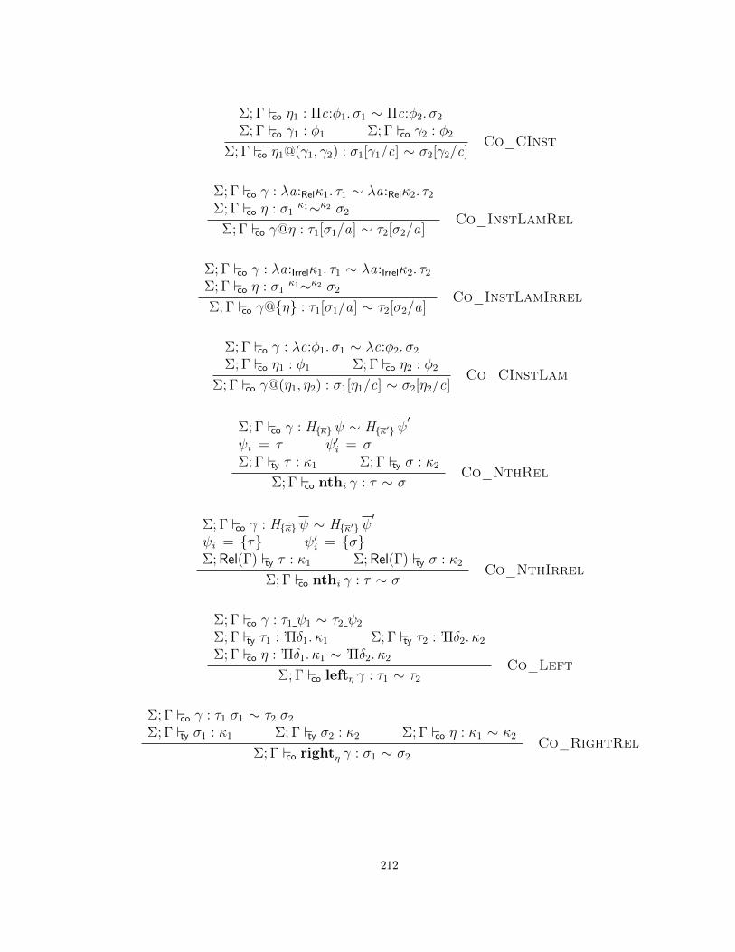
Σ; Γ co η1 : Πc:φ1. σ1 ∼ Πc:φ2. σ2

Σ; Γ co γ1 : φ1 Σ; Γ co γ2 : φ2

Σ; Γ co η1@(γ1, γ2) : σ1[γ1/c] ∼ σ2[γ2/c]Co_CInst

Σ; Γ co γ : λa:Relκ1. τ1 ∼ λa:Relκ2. τ2

Σ; Γ co η : σ1κ1∼κ2 σ2

Σ; Γ co γ@η : τ1[σ1/a] ∼ τ2[σ2/a]Co_InstLamRel

Σ; Γ co γ : λa:Irrelκ1. τ1 ∼ λa:Irrelκ2. τ2

Σ; Γ co η : σ1κ1∼κ2 σ2

Σ; Γ co γ@η : τ1[σ1/a] ∼ τ2[σ2/a]Co_InstLamIrrel

Σ; Γ co γ : λc:φ1. σ1 ∼ λc:φ2. σ2

Σ; Γ co η1 : φ1 Σ; Γ co η2 : φ2

Σ; Γ co γ@(η1, η2) : σ1[η1/c] ∼ σ2[η2/c]Co_CInstLam

Σ; Γ co γ : Hκ ψ ∼ Hκ′ ψ′

ψi = τ ψ′i = σΣ; Γ ty τ : κ1 Σ; Γ ty σ : κ2

Σ; Γ co nthi γ : τ ∼ σCo_NthRel

Σ; Γ co γ : Hκ ψ ∼ Hκ′ ψ′

ψi = τ ψ′i = σΣ; Rel(Γ) ty τ : κ1 Σ; Rel(Γ) ty σ : κ2

Σ; Γ co nthi γ : τ ∼ σCo_NthIrrel

Σ; Γ co γ : τ1 ψ1 ∼ τ2 ψ2

Σ; Γ ty τ1 : ’Πδ1. κ1 Σ; Γ ty τ2 : ’Πδ2. κ2

Σ; Γ co η : ’Πδ1. κ1 ∼ ’Πδ2. κ2

Σ; Γ co leftη γ : τ1 ∼ τ2

Co_Left

Σ; Γ co γ : τ1 σ1 ∼ τ2 σ2

Σ; Γ ty σ1 : κ1 Σ; Γ ty σ2 : κ2 Σ; Γ co η : κ1 ∼ κ2

Σ; Γ co rightη γ : σ1 ∼ σ2

Co_RightRel

212

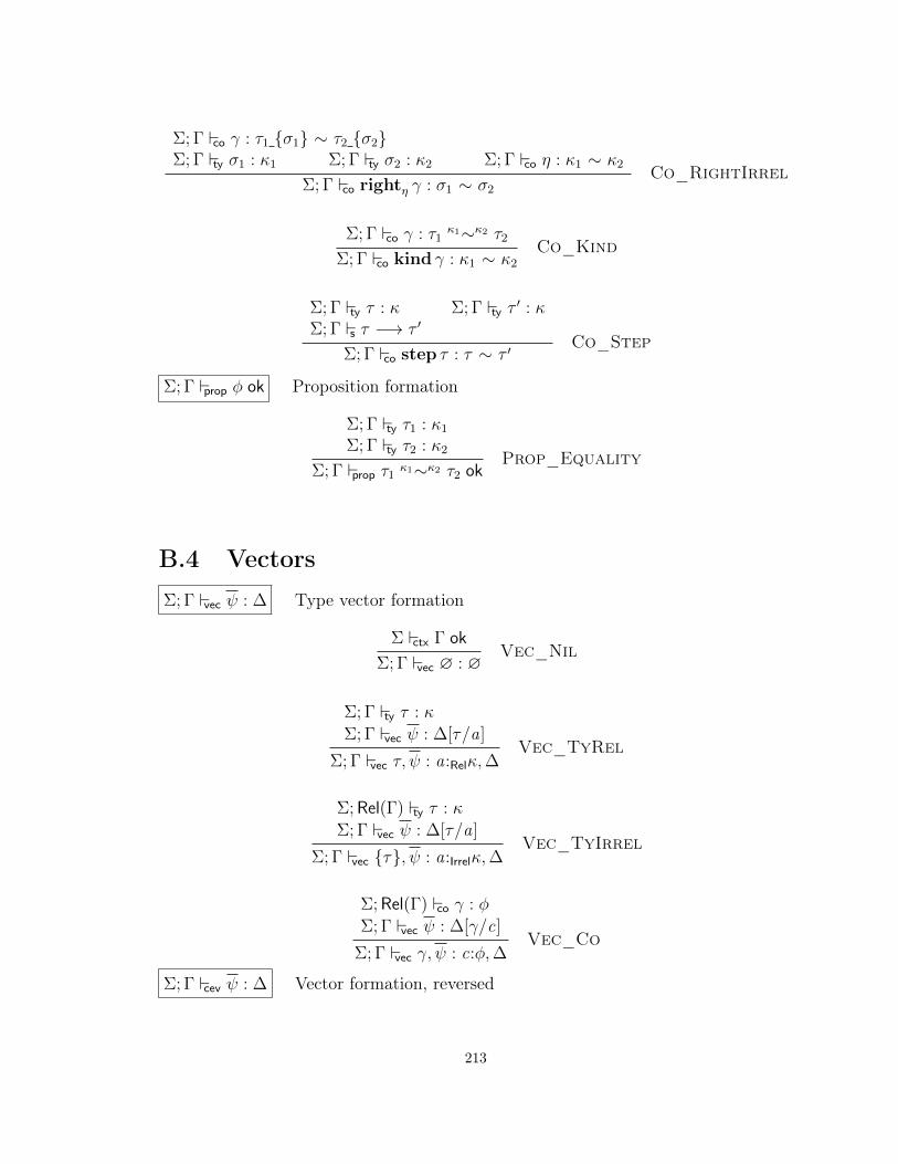
Σ; Γ co γ : τ1 σ1 ∼ τ2 σ2Σ; Γ ty σ1 : κ1 Σ; Γ ty σ2 : κ2 Σ; Γ co η : κ1 ∼ κ2

Σ; Γ co rightη γ : σ1 ∼ σ2

Co_RightIrrel

Σ; Γ co γ : τ1κ1∼κ2 τ2

Σ; Γ co kind γ : κ1 ∼ κ2

Co_Kind

Σ; Γ ty τ : κ Σ; Γ ty τ′ : κ

Σ; Γ s τ −→ τ ′

Σ; Γ co step τ : τ ∼ τ ′Co_Step

Σ; Γ prop φ ok Proposition formation

Σ; Γ ty τ1 : κ1

Σ; Γ ty τ2 : κ2

Σ; Γ prop τ1κ1∼κ2 τ2 ok

Prop_Equality

B.4 VectorsΣ; Γ vec ψ : ∆ Type vector formation

Σ ctx Γ ok

Σ; Γ vec ∅ : ∅Vec_Nil

Σ; Γ ty τ : κ

Σ; Γ vec ψ : ∆[τ/a]

Σ; Γ vec τ, ψ : a:Relκ,∆Vec_TyRel

Σ; Rel(Γ) ty τ : κ

Σ; Γ vec ψ : ∆[τ/a]

Σ; Γ vec τ, ψ : a:Irrelκ,∆Vec_TyIrrel

Σ; Rel(Γ) co γ : φ

Σ; Γ vec ψ : ∆[γ/c]

Σ; Γ vec γ, ψ : c:φ,∆Vec_Co

Σ; Γ cev ψ : ∆ Vector formation, reversed

213

Σ ctx Γ ok

Σ; Γ cev ∅ : ∅Cev_Nil

Σ; Γ cev ψ : ∆

Σ; Γ ty τ : κ[ψ/dom(∆)]

Σ; Γ cev ψ, τ : ∆, a:RelκCev_TyRel

Σ; Γ cev ψ : ∆

Σ; Rel(Γ) ty τ : κ[ψ/dom(∆)]

Σ; Γ cev ψ, τ : ∆, a:IrrelκCev_TyIrrel

Σ; Γ cev ψ : ∆

Σ; Rel(Γ) co γ : φ[ψ/dom(∆)]

Σ; Γ cev ψ, γ : ∆, c:φCev_Co

B.5 Contexts

sig Σ ok Signature formation

sig ∅ okSig_Nil

Σ ctx a:Irrelκ ok T # Σ

sig Σ,T :(a:κ) okSig_ADT

T :(a:κ) ∈ Σ Σ ctx a:Irrelκ,∆ ok K # Σ

sig Σ,K :(∆;T ) okSig_DataCon

Σ ctx Γ ok Context formation

sig Σ ok

Σ ctx ∅ okCtx_Nil

Σ; Rel(Γ) ty κ : Type a # Γ Σ ctx Γ ok

Σ ctx Γ, a:ρκ okCtx_TyVar

214

Σ; Rel(Γ) prop φ ok c # Γ Σ ctx Γ ok

Σ ctx Γ, c:φ okCtx_CoVar

B.6 Small-step operational semantics

Σ; Γ s σ −→ σ′ Small-step operational semantics

Σ; Γ s (λa:Relκ. σ1)˜σ2 −→ σ1[σ2/a]S_BetaRel

Σ; Γ s (λa:Irrelκ. v1)˜σ2 −→ v1[σ2/a]S_BetaIrrel

Σ; Γ s (λc:φ. σ)˜γ −→ σ[γ/c]S_CBeta

alti = H → τ0

Σ; Γ s caseκHτ ψ of alt −→ τ0 ψ 〈Hτ ψ〉S_Match

alti = _→ σ no alternative in alt matches HΣ; Γ s caseκHτ ψ of alt −→ σ

S_Default

alti = _→ σ no alternative in alt matches HΣ; Γ s caseκHτ ψ B γ of alt −→ σ

S_DefaultCo

τ = λa:Relκ. σ

Σ; Γ s fix τ −→ σ[fix τ/a]S_Unroll

Σ; Γ s (v B γ1)B γ2 −→ v B (γ1 # γ2)S_Trans

Σ; Γ, a:Irrelκ s σ −→ σ′

Σ; Γ s λa:Irrelκ. σ −→ λa:Irrelκ. σ′S_IrrelAbs_Cong

Σ; Γ s σ −→ σ′

Σ; Γ s σ ψ −→ σ′ ψS_App_Cong

215

Σ; Γ s σ −→ σ′

Σ; Γ s σ B γ −→ σ′ B γS_Cast_Cong

Σ; Γ s σ −→ σ′

Σ; Γ s caseτ σ of alt −→ caseτ σ′ of altS_Case_Cong

Σ; Γ s τ −→ τ ′

Σ; Γ s fix τ −→ fix τ ′S_Fix_Cong

Σ; Rel(Γ) co γ0 : Πa:Relκ. σ ∼ Πa:Relκ′. σ′

γ1 = sym (argk γ0) γ2 = γ0@(τ B γ1 ≈sym γ1 τ)

Σ; Γ s (v B γ0) τ −→ v (τ B γ1)B γ2

S_PushRel

Σ; Rel(Γ) co γ0 : Πa:Irrelκ. σ ∼ Πa:Irrelκ′. σ′

γ1 = sym (argk γ0) γ2 = γ0@(τ B γ1 ≈sym γ1 τ)

Σ; Γ s (v B γ0) τ −→ v τ B γ1B γ2

S_PushIrrel

Σ; Rel(Γ) co γ0 : Πc:φ. σ ∼ Πc:φ′. σ′

γ1 = argk1 γ0 γ2 = argk2 γ0

η′ = γ1 # η # sym γ2 γ3 = γ0@(η′, η)

Σ; Γ s (v B γ0) η −→ v η′ B γ3

S_CPush

γ1 =˜Πa:Irrel〈κ〉. γ γ2 = τ1 ≈〈Type〉 τ2

τ1 =˜Πa:Irrelκ. (κ1[a B sym 〈κ〉/a]) τ2 =

˜Πa:Irrelκ. κ1

Σ; Γ s λa:Irrelκ. (v B γ) −→ (λa:Irrelκ. v)B (γ1 # γ2)S_APush

γ1 = γ0@(a ≈γ2 a B γ2) # sym γ2

γ2 = argk γ0

Σ; Γ s fix ((λa:Relκ. σ)B γ0) −→ (fix (λa:Relκ. (σ B γ1)))B γ2

S_FPush

216

Σ tc H : a:Irrelκ; ∆;H ′ ∆ = ∆1,∆2 n = |∆2|κ = ’Πa:Irrelκ,∆.H

′ a

σ = ’Π(∆2[τ/a][ψ/dom(∆1)]).H ′ τ

σ′ = ’Π(∆2[τ ′/a][ψ′/dom(∆1)]).H ′ τ ′

Σ; Rel(Γ) co η : σ ∼ σ′

Σ; Rel(Γ) vec τ′ : a:Relκ

∀i , γi = build_kpush_co(〈κ〉@(nths (resn η));ψ1...i−1)∀i , ψ′i = cast_kpush_arg(ψi ; γi)

H → κ′ ∈ alt

Σ; Γ s caseκ0 (Hτ ψ)B η of alt −→ caseκ0 Hτ ′ ψ′of alt

S_KPush

B.7 Consistencyτ1 ∝ τ2 Type compatibility

τ1 is not a valueτ1 ∝ τ2

C_NonValue1

τ2 is not a valueτ1 ∝ τ2

C_NonValue2

Hτ ψ ∝ Hτ ′ ψ′ C_TyCon

τ ∝ τ ′

Πa:ρκ. τ ∝ Πa:ρκ′. τ ′C_PiTy

Πc:φ. τ ∝ Πc:φ′. τ ′C_PiCo

λδ. τ ∝ λδ′. τ ′C_Lam

τ τ ′ Parallel reduction over erased types

τ τR_Refl

217

τ τ ′

Hτ Hτ ′R_Con

τ τ ′ σ σ′

τ σ τ ′ σ′R_AppRel

τ τ ′ σ σ′

τ σ τ ′ σ′R_AppIrrel

τ τ ′

τ • τ ′ •R_CApp

δ δ′ τ τ ′

Πδ. τ Πδ′. τ ′R_Pi

κ κ′ τ τ ′ σ σ′

caseκ τ of π → σ caseκ′ τ ′ of π → σ′R_Case

δ δ′ τ τ ′

λδ. τ λδ′. τ ′R_Lam

τ τ ′

fix τ fix τ ′R_Fix

τ τ ′

absurd • τ absurd • τ ′R_Absurd

τ1 τ ′1 τ2 τ ′2(λa:Relκ. τ1)˜τ2 τ ′1[τ ′2/a]

R_BetaRel

τ1 τ ′1 τ2 τ ′2(λa:Irrelκ. τ1)˜τ2 τ ′1[τ ′2/a]

R_BetaIrrel

τ τ ′

(λ•:φ. τ)˜• τ ′R_CBeta

218

alti = H → τ0 ψ ψ′

τ0 τ ′0

caseκHτ ψ of alt τ ′0 ψ′ •

R_Match

alti = _→ σ no alternative in alt matches H σ σ′

caseκHτ ψ of alt σ′R_Default

σ σ′ κ κ′

fix (λa:Relκ. σ) σ′[fix (λa:Relκ′. σ′)/a]R_Unroll

δ δ′ Parallel reduction of binders

κ κ′

a:ρκ a:ρκ′R_TyBinder

τ τ ′ κ1 κ′1 κ2 κ′2 σ σ′

•:τ κ1∼κ2 σ •:τ ′ κ′1∼κ′2 σ′R_CoBinder

γ γ′ “Reduction” of erased coercion

• •R_ErasedCo

B.8 Small-step operational semantics of erased ex-pressions

e −→ e ′ Single-step operational semantics of expressions

(λa.e1) e2 −→ e1[e2/a]E_Beta

(λ•.e) • −→ eE_CBeta

ealti = H → e

caseH y of ealt −→ e y •E_Match

ealti = _→ e no alternative in ealt matches HcaseH y of ealt −→ e

E_Default

219

fix (λa.e) −→ e[fix (λa.e)/a]E_Unroll

e −→ e ′

e y −→ e ′ yE_App_Cong

e −→ e ′

case e of ealt −→ case e ′ of ealtE_Case_Cong

e −→ e ′

fix e −→ fix e ′E_Fix_Cong

220

Appendix C

Proofs about Pico

You may find the full grammar for Pico in Figure 5.1 on page 76 and its notationconventions in Figure 5.2 on page 77. The definition for values is in Section 5.7.1 andof the # operator in Section 5.8.5.2.

C.1 Auxiliary definitionsDefinition C.1 (Free variables). Define fv to be a function extracting free variables,overloaded to work over types τ , coercions γ, propositions φ, vectors ψ, alternativesalt , and telescopes ∆. The definitions are entirely standard.

Definition C.2 (Context extension). Define the relation Γ ⊆ Γ′ to mean that Γ is a(not necessarily contiguous) subsequence of Γ′.

C.2 Structural properties

C.2.1 Relevant contexts

Lemma C.3 (dom/Rel). dom(Rel(Γ)) = dom(Γ)

Proof. By its definition Rel(Γ) binds the same variables as Γ.

Lemma C.4 (Subsequence/Rel). If Γ ⊆ Γ′ then Rel(Γ) ⊆ Rel(Γ′).

Proof. By the definitions of ⊆ and Rel.

Lemma C.5 (Rel is idempotent). Rel(Rel(Γ)) = Rel(Γ)

Proof. By the definition of Rel.

Lemma C.6 (Increasing relevance). Let Γ and Γ′ be the same except that somebindings in Γ′ are labeled Rel where those same bindings in Γ are labeled Irrel.

221

1. If Σ; Γ ty τ : κ, then Σ; Γ′ ty τ : κ.

2. If Σ; Γ co γ : φ, then Σ; Γ′ co γ : φ.

3. If Σ; Γ prop φ ok, then Σ; Γ′ prop φ ok.

4. If Σ; Γ;σ0 `τ0alt alt : κ, then Σ; Γ′;σ0 `τ0alt alt : κ.

5. If Σ; Γ vec ψ : ∆, then Σ; Γ′ vec ψ : ∆.

6. If Σ ctx Γ ok, then Σ ctx Γ′ ok.

7. If Σ; Γ s τ −→ τ ′, then Σ; Γ′ s τ −→ τ ′.

Proof. By straightforward mutual induction, appealing to Lemma C.5.

C.2.2 Regularity, Part I

Lemma C.7 (Type variable kinds). If Σ ctx Γ ok and a:ρκ ∈ Γ, then there exists Γ′

such that Γ′ ⊆ Rel(Γ) and Σ; Γ′ ty κ : Type. Furthermore, the size of the derivationof Σ; Γ′ ty κ : Type is smaller than that of Σ ctx Γ ok.

Proof. Straightforward induction on Σ ctx Γ ok.

Lemma C.8 (Coercion variable kinds). If Σ ctx Γ ok and c:φ ∈ Γ, then there existsΓ′ such that Γ′ ⊆ Rel(Γ) and Σ; Γ′ prop φ ok. Furthermore, the size of the derivationof Σ; Γ′ prop φ ok is smaller than that of Σ ctx Γ ok.

Proof. Straightforward induction on Σ ctx Γ ok.

Lemma C.9 (Context regularity). If:

1. Σ; Γ ty τ : κ, OR

2. Σ; Γ co γ : φ, OR

3. Σ; Γ prop φ ok, OR

4. Σ; Γ;σ0 `τ0alt alt : κ, OR

5. Σ; Γ vec ψ : ∆, OR

6. Σ ctx Γ ok

Then Σ ctx prefix(Γ) ok and sig Σ ok, where prefix(Γ) is an arbitrary prefix of Γ.Furthermore, both resulting derivations are no larger than the input derivations.

Proof. Straightforward mutual induction.

222

C.2.3 Weakening

Lemma C.10 (Weakening). Assume Σ ctx Γ′ ok and Γ ⊆ Γ′.

1. If Σ; Γ ty τ : κ then Σ; Γ′ ty τ : κ.2. If Σ; Γ co γ : φ, then Σ; Γ′ co γ : φ.3. If Σ; Γ prop φ ok, then Σ; Γ′ prop φ ok.4. If Σ; Γ;σ0 `τ0alt alt : κ, then Σ; Γ′;σ0 `τ0alt alt : κ.5. If Σ; Γ vec ψ : ∆, then Σ; Γ′ vec ψ : ∆.6. If Σ ctx Γ,∆ ok, then Σ ctx Γ′,∆ ok.7. If Σ; Γ s τ −→ τ ′, then Σ; Γ′ s τ −→ τ ′.

Proof. By straightforward mutual induction, appealing to Lemma C.4, Lemma C.6(in order to be able to use the induction hypothesis in, e.g., Ty_AppIrrel), andLemma C.9 (in order to use the induction hypothesis in, e.g., Ty_Pi).

Lemma C.11 (Strengthening). Assume Γ′ ⊆ Γ and the variablesdom(Γ) \dom(Γ′) are never used.

1. If Σ; Γ ty τ : κ then Σ; Γ′ ty τ : κ.2. If Σ; Γ co γ : φ, then Σ; Γ′ co γ : φ.3. If Σ; Γ prop φ ok, then Σ; Γ′ prop φ ok.4. If Σ; Γ;σ0 `τ0alt alt : κ, then Σ; Γ′;σ0 `τ0alt alt : κ.5. If Σ; Γ vec ψ : ∆, then Σ; Γ′ vec ψ : ∆.6. If Σ ctx Γ ok, then Σ ctx Γ′ ok.7. If Σ; Γ s τ −→ τ ′, then Σ; Γ′ s τ −→ τ ′.

Proof. Similar to previous proof.

C.2.4 Scoping

Lemma C.12 (Scoping).

1. If Σ; Γ ty τ : κ, then fv(τ) ⊆ dom(Γ) and fv(κ) ⊆ dom(Γ).2. If Σ; Γ co γ : φ, then fv(γ) ⊆ dom(Γ) and fv(φ) ⊆ dom(Γ).3. If Σ; Γ prop φ ok, then fv(φ) ⊆ dom(Γ).4. If Σ; Γ;σ0 `τ0alt H → τ : κ, then fv(τ) ⊆ dom(Γ).5. If Σ; Γ vec ψ : ∆, then fv(ψ) ⊆ dom(Γ) and fv(∆) ⊆ dom(Γ).6. If Σ ctx Γ ok, then fv(Γ) = ∅.7. If sig Σ ok and Σ tc H : ∆1; ∆2;H ′, then fv(∆1) = ∅ and fv(∆2) ⊆ dom(∆1).

Proof. By straightforward mutual induction, appealing to Lemma C.3, Lemma C.7,Lemma C.8, and Lemma C.9.

223

C.3 UnificationWe assume the following properties of our unification algorithm.

Property C.13 (Domain of match). If matchV(τ 1; τ 2) = Just θ, then θ = ψ/z forsome ψ and z with V = z. In other words, the domain of the substitution returnedby a successful use of match is the variables V passed into match.

Property C.14 (match is sound). If matchV(τ 1; τ 2) = Just θ, then τ 1[θ] = τ 2.

Property C.15 (match/substitution). If matchV(τ 1; τ 2) = Just θ and dom(θ0)∩V =∅, matchV(τ 1[θ0]; τ 2[θ0]) = Just θ′ for some θ′.

C.4 DeterminacyLemma C.16 (Uniqueness of signatures). Assume sig Σ ok.

1. If T :(a:κ1) ∈ Σ and T :(a:κ2) ∈ Σ, then κ1 = κ2.

2. If K :(∆1;T1) ∈ Σ and K :(∆2;T2) ∈ Σ, then ∆1 = ∆2 and T1 = T2.

Proof. By the freshness conditions on sig Σ ok.

Lemma C.17 (Uniqueness of contexts). Assume Σ ctx Γ ok.

1. If a:ρ1κ1 ∈ Γ and a:ρ2κ2 ∈ Γ, then ρ1 = ρ2 and κ1 = κ2.

2. If c:φ1 ∈ Γ and c:φ2 ∈ Γ, then φ1 = φ2.

Proof. By the freshness conditions on Σ ctx Γ ok.

Lemma C.18 (Determinacy of type constants). If sig Σ ok, Σ tc H : ∆1; ∆′1;H1, andΣ tc H : ∆2; ∆′2;H2, then ∆1 = ∆2, ∆′1 = ∆′2, and H1 = H2.

Proof. From Lemma C.16.

Lemma C.19 (Values do not step). There exists no τ such that Σ; Γ s v −→ τ .

Proof. By induction on the structure of v .

Lemma C.20 (Determinacy).

1. If Σ; Γ ty τ : κ1 and Σ; Γ ty τ : κ2, then κ1 = κ2.

2. If Σ; Γ co γ : φ1 and Σ; Γ co γ : φ2, then φ1 = φ2.

3. If Σ; Γ s τ −→ σ1 and Σ; Γ s τ −→ σ2, then σ1 = σ2.

Proof. By mutual induction, appealing to Lemma C.17, Lemma C.18 (which requiresa use of Lemma C.9 first), and Lemma C.19.

224

C.5 VectorsLemma C.21. If Σ; Γ ty τ : κ and Σ; Γ cev ψ : ∆[τ/a], then Σ; Γ cev τ, ψ : a:Relκ,∆.

Proof. By induction on Σ; Γ cev ψ : ∆[τ/a].

Case Cev_Nil: In this case, ψ and ∆ are both empty, and so we are done byCev_Nil and Cev_TyRel.

Case Cev_TyRel: We now have ψ = ψ′, σ and ∆ = ∆′, b:Relκ0, with Σ; Γ ty σ :

κ0[τ/a][ψ′/dom(∆′)] and Σ; Γ cev ψ

′: ∆′[τ/a]. The induction hypothesis gives

us Σ; Γ cev τ, ψ′: a:Relκ,∆

′. We are done by Cev_TyRel.

Other cases: Similar.

Lemma C.22. If Σ; Rel(Γ) ty τ : κ and Σ; Γ cev ψ : ∆[τ/a], then Σ; Γ cev τ, ψ :a:Irrelκ,∆.

Proof. Similar to previous proof.

Lemma C.23. If Σ; Rel(Γ) co γ : φ and Σ; Γ cev ψ : ∆[γ/c], then Σ; Γ cev γ, ψ :c:φ,∆.

Proof. Similar to previous proof.

Lemma C.24. If Σ; Γ vec ψ : ∆ and Σ; Γ ty τ : κ[ψ/dom(∆)], then Σ; Γ vec ψ, τ :∆, a:Relκ.

Proof. By induction on Σ; Γ vec ψ : ∆.

Case Vec_Nil: In this case, ψ and ∆ are both empty, and so we are done byVec_Nil and Vec_TyRel.

Case Vec_TyRel: We now have ψ = σ, ψ′ and ∆ = b:Relκ0,∆

′ with Σ; Γ ty

σ : κ0 and Σ; Γ vec ψ′

: ∆′[σ/b]. We know, by assumption, that Σ; Γ ty τ :

κ[ψ/dom(∆)]. This expands to Σ; Γ ty τ : κ[σ/b][ψ′/dom(∆′)] (noting that

Lemma C.12 assures us that σ has no variables in dom(∆′) free). We can thususe the induction hypothesis to get Σ; Γ vec ψ

′, τ : ∆′[σ/b], a:Relκ[σ/b], or,

equivalently, Σ; Γ vec ψ′, τ : (∆′, a:Relκ)[σ/b]. We are done by Vec_TyRel.

Other cases: Similar.

Lemma C.25. If Σ; Γ vec ψ : ∆ and Σ; Rel(Γ) ty τ : κ[ψ/dom(∆)], then Σ; Γ vec

ψ, τ : ∆, a:Irrelκ.

225

Proof. Similar to previous proof.

Lemma C.26. If Σ; Γ vec ψ : ∆ and Σ; Rel(Γ) co γ : φ[ψ/dom(∆)], then Σ; Γ vec

ψ, γ : ∆, c:φ.

Proof. Similar to previous proof.

Lemma C.27 (Vec/Cev). We have Σ; Γ vec ψ : ∆ if and only if Σ; Γ cev ψ : ∆.

Proof. We’ll prove the forward direction first, by induction on the typing derivation:

Case Vec_Nil: We are done by Cev_Nil.

Case Vec_TyRel: By the induction hypothesis and Lemma C.21.

Case Vec_TyIrrel: By the induction hypothesis and Lemma C.22.

Case Vec_Co: By the induction hypothesis and Lemma C.23.

The reverse direction is similar, appealing to Lemma C.24, Lemma C.25, andLemma C.26.

Lemma C.28 (Vector lengths). If Σ; Γ vec ψ : ∆, then |ψ| = |∆|.

Proof. Straightforward induction on Σ; Γ vec ψ : ∆.

Lemma C.29 (Vector kinds). If Σ; Γ vec ψ : ∆, then for every ψ ∈ ψ, we have oneof the following:

1. ψ = τ and Σ; Γ ty τ : κ for some κ

2. ψ = τ and Σ; Rel(Γ) ty τ : κ for some κ

3. ψ = γ and Σ; Rel(Γ) co γ : φ for some φ

The resulting derivation is smaller than the input derivation.

Proof. Straightforward induction on Σ; Γ vec ψ : ∆.

Lemma C.30 (Application inversion). If Σ; Γ ty τ ψ : κ where ψ = ψ0, ψ1, thenΣ; Γ ty τ ψ0 : ?Π∆. κ0, Σ; Γ vec ψ1 : ∆ and κ = κ0[ψ1/dom(∆)].

Proof. Straightforward induction on ψ1.

Lemma C.31 (Telescope application). If Σ; Γ ty τ : ?Π∆. σ and Σ; Γ vec ψ : ∆, thenΣ; Γ ty τ ψ : σ[ψ/dom(∆)].

Proof. By straightforward induction on Σ; Γ vec ψ : ∆.

Lemma C.32 (Telescope instantiation). If Σ; Γ co η : ’Π∆. σ ∼ ’Π∆′. σ′, (∀i ,Σ; Γ co

γi : τi ∼ τ ′i ), Σ; Γ vec τ : ∆, and Σ; Γ vec τ′ : ∆′, then Σ; Γ co η@γ : σ[τ/dom(∆)] ∼

σ′[τ ′/dom(∆′)].

226

Proof. By induction on the structure of the list γ.

Case γ = ∅: By Lemma C.28, we can see that ∆ and ∆′ must both be empty. Weare done by assumption.

Case γ = γ0, γ1: In this case, we know Σ; Γ vec τ0, τ 1 : ∆ and thus that ∆ =a:Relκ0,∆1 with Σ; Γ ty τ0 : κ0 and Σ; Γ vec τ 1 : ∆1[τ0/a]. Similarly, we haveΣ; Γ ty τ

′0 : κ′0 and Σ; Γ vec τ

′1 : ∆′1[τ

′0/a]. We must show Σ; Γ co (η@γ0)@γ1 :

σ[τ0/a, τ 1/dom(∆1)] ∼ σ′[τ ′0/a, τ′1/dom(∆′1)]. We can rewrite our assumption

(expanding ∆ and ∆′) to be Σ; Γ co η : ’Πa:Relκ0,∆1. σ ∼ ’Πa:Relκ′0,∆

′1. σ

′ andthus derive Σ; Γ co η@γ0 : ’Π(∆1[τ0/a]). (σ[τ0/a]) ∼ ’Π(∆′1[τ

′0/a]). (σ′[τ ′0/a]).

We can then use the induction hypothesis to get Σ; Γ co (η@γ0)@γ :σ[τ0/a][τ 1/dom(∆1)] ∼ σ′[τ ′0/a][τ ′1/dom(∆′1)], which (noting that τ0 cannothave any of the dom(∆1) free) is what we wish to prove.

Remark. The above Lemma C.32 could be made more general, to work with˜Π as well

as ’Π. However, doing so would make the statement and proof more cluttered, and itis only ever needed with ’Π.

C.6 SubstitutionLemma C.33 (Value substitution). If v is a value with a free variable a, then v [σ/a]is also a value.

Proof. By the definition of values.

Lemma C.34 (Substitution/erasure). bτc[bσc/a] = bτ [σ/a]c

Proof. By induction on the structure of τ .

Lemma C.35 (Type substitution). Assume Σ; Γ ty σ : κ.

1. If Σ; Γ, a:ρκ,Γ′

ty τ : κ0, then Σ; Γ,Γ′[σ/a] ty τ [σ/a] : κ0[σ/a].

2. If Σ; Γ, a:ρκ,Γ′

co γ : φ, then Σ; Γ,Γ′[σ/a] co γ[σ/a] : φ[σ/a].

3. If Σ; Γ, a:ρκ,Γ′

prop φ ok, then Σ; Γ,Γ′[σ/a] prop φ[σ/a] ok.

4. If Σ; Γ, a:ρκ,Γ′;σ0 `τ0alt alt : κ, then Σ; Γ,Γ′[σ/a];σ0[σ/a] `τ0[σ/a]

alt alt [σ/a] : κ[σ/a].

5. If Σ; Γ, a:ρκ,Γ′

vec ψ : ∆, then Σ; Γ,Γ′[σ/a] vec ψ[σ/a] : ∆[σ/a].

6. If Σ ctx Γ, a:ρκ,Γ′ ok, then Σ ctx Γ,Γ′[σ/a] ok.

7. If Σ; Γ, a:ρκ,Γ′

s τ −→ τ ′, then Σ; Γ,Γ′[σ/a] s τ [σ/a] −→ τ ′[σ/a].

Proof. By mutual induction. Some interesting cases are below.

227

Case Ty_Var: Here, we know τ is some variable b. There are three cases toconsider:

Case b:Relκ0 ∈ Γ: We must derive Σ; Γ,Γ′[σ/a] ty b : κ0[σ/a]. We will useTy_Var. We establish Σ ctx Γ,Γ′[σ/a] ok by the induction hypothesis.Scoping (Lemma C.12) tells us that a 6∈ fv(κ0), and so we are done by thefact that b:Relκ0 ∈ Γ.

Case b = a: By weakening (Lemma C.10).Case b:Relκ0 ∈ Γ′: Once again, we get Σ ctx Γ,Γ′[σ/a] ok by the induction

hypothesis. Furthermore, we get b:Relκ0[σ/a] ∈ Γ′[σ/a] from b:Relκ0 ∈ Γ′.

Case Ty_Con: By Lemma C.12, Lemma C.9, and induction.

Case Alt_Match: We adopt the metavariable names from the rule:

Σ tc H : ∆1; ∆2;H ′ ∆3,∆4 = ∆2[σ/dom(∆1)]dom(∆4) = dom(∆′)matchdom(∆3)(types(∆4); types(∆′)) = Just θΣ; Γ ty τ : ?Π∆3, c:τ0 ∼ Hσ dom(∆3). κ

Σ; Γ; ’Π∆′.H ′ σ `τ0alt H → τ : κAlt_Match

We will use Alt_Match to prove our desired conclusion. Several premises areunchanged. The remaining ones we will have to prove:

∆′3,∆′4 = ∆2[σ[σ/a]/dom(∆1)]: By our choice of ∆′3 = ∆3[σ/a] and ∆′4 =

∆4[σ/a].matchdom(∆3)(types(∆4[σ/a]); types(∆′[σ/a])) = Just θ′: We can freely choose

θ′, but we still need to make sure that the match succeeds. This is byProperty C.15.

Case Co_Var: Similar to Ty_Var.

Case Co_PiTy: We adopt the metavariable names from the rule (renaming thevariable to be substituted to b):

Σ; Γ co η : κ1Type∼Type κ2

Σ; Γ, a:Relκ1 co γ : σ1Type∼Type σ2

Σ; Γ co Πa:ρη. γ : (Πa:ρκ1. σ1) ∼ (Πa:ρκ2. (σ2[a B sym η/a]))Co_PiTy

The induction hypothesis gives us:

• Σ; Γ,Γ′[σ/b] co η[σ/b] : κ1[σ/b] ∼ κ2[σ/b]

• Σ; Γ,Γ′[σ/b], a:Relκ1[σ/b] co γ[σ/b] : σ1[σ/b] ∼ σ2[σ/b]

228

By Co_PiTy, we get

Σ; Γ,Γ′[σ/b] co Πa:ρη[σ/b]. γ[σ/b] :

(Πa:ρκ1[σ/b]. σ1[σ/b]) ∼ (Πa:ρκ2[σ/b]. (σ2[σ/b][a B sym η[σ/b]/a]))

All that remains to show is that σ2[σ/b][a B sym η[σ/b]/a] = σ2[a Bsym η/a][σ/b], but this follows from the fact that a # σ, guaranteed by theBarendregt convention. We are done with this case.

Case Co_PiCo: We adopt the metavariable names from the rule:

Σ; Γ co η1 : τ1 ∼ τ2 Σ; Γ co η2 : σ1 ∼ σ2

Σ; Γ, c:τ1 ∼ σ1 co γ : κ1Type∼Type κ2 c # γ

η3 = η1 # c # sym η2

Σ; Γ co Πc:(η1, η2). γ : (Πc:τ1 ∼ σ1. κ1) ∼ (Πc:τ2 ∼ σ2. (κ2[η3/c]))Co_PiCo

For the most part, this follows the pattern of case Co_PiTy, but we must makesure that c # γ[σ/a]. This fact follows from the Barendregt convention, whichasserts that c cannot appear in σ.

Other cases: By the induction hypothesis, using Lemma C.33 for certain step rules,and using the Barendregt convention to rearrange substitutions (as in theCo_PiTy case).

Lemma C.36 (Coercion substitution). Assume Σ; Γ co γ : φ.

1. If Σ; Γ, c:φ,Γ′ ty τ : κ0, then Σ; Γ,Γ′[γ/c] ty τ [γ/c] : κ0[γ/c].

2. If Σ; Γ, c:φ,Γ′ co η : φ′, then Σ; Γ,Γ′[γ/c] co η[γ/c] : φ′[γ/c].

3. If Σ; Γ, c:φ,Γ′ prop φ′ ok, then Σ; Γ,Γ′[γ/c] prop φ

′[γ/c] ok.

4. If Σ; Γ, c:φ,Γ′;σ0 `τ0alt alt : κ, then Σ; Γ,Γ′[γ/c];σ0[γ/c] `τ0[γ/c]alt alt [γ/c] : κ[γ/c].

5. If Σ; Γ, c:φ,Γ′ vec ψ : ∆, then Σ; Γ,Γ′[γ/c] vec ψ[γ/c] : ∆[γ/c].

6. If Σ ctx Γ, c:φ,Γ′ ok, then Σ ctx Γ,Γ′[γ/c] ok.

7. If Σ; Γ, c:φ,Γ′ s τ −→ τ ′, then Σ; Γ,Γ′[γ/c] s τ [γ/c] −→ τ ′[γ/c].

Proof. Similar to proof for Lemma C.35.

Lemma C.37 (Vector substitution). If Σ; Γ vec ψ : ∆ and Σ; Γ,∆,Γ′ ty τ : κ, thenΣ; Γ,Γ′[ψ/dom(∆)] ty τ [ψ/dom(∆)] : κ[ψ/dom(∆)].

Proof. By induction on the structure of ∆.

Case ∆ = ∅: By assumption.

229

Case ∆ = a0:Relκ0,∆′: We know ψ = σ0, ψ

′, Σ; Γ ty σ0 : κ0, and Σ; Γ vec ψ′

:∆′[σ0/a]. Lemma C.35 tells us Σ; Γ,∆′[σ0/a],Γ′[σ0/a] ty τ [σ0/a] : κ[σ0/a]. Weare done by a use of the induction hypothesis.

Other cases: Similar.

C.7 Type constantsLemma C.38 (Type-in-type). If sig Σ ok, then Σ;∅ ty Type : Type.

Proof. Working backward, use Ty_Con so that we must show the following:

Σ tc Type : ∅;∅; Type: By Tc_Type.

Σ ctx ∅ ok: By Ctx_Nil.

Σ;∅ vec ∅ : ∅: By Vec_Nil.

We are thus done.

Lemma C.39 (Telescopes). If Σ ctx Γ,∆ ok, then Σ; Γ,∆ vec dom(∆) : ∆.

Proof. Proceed by induction on the structure of ∆.

Case ∆ = ∅: By Vec_Nil.

Case ∆ = a:Relκ,∆′: We must show Σ; Γ, a:Relκ,∆

′vec a, dom(∆′) : a:Relκ,∆

′. ByVec_TyRel, we must show Σ; Γ, a:Relκ,∆

′ty a : κ and Σ; Γ, a:Relκ,∆

′vec

dom(∆′) : ∆′. The first is by Ty_Var and the second is by the inductionhypothesis.

Other cases: Similar.

Lemma C.40 (Type constant telescopes). If sig Σ ok and Σ tc H : ∆1; ∆2;H ′, thenΣ ctx ∆1,∆2 ok.

Proof. By case analysis on Σ tc H : ∆1; ∆2;H ′.

Case Tc_ADT: Here ∆1 = ∅ and ∆2 = a:Relκ We see that Σ ctx a:Irrelκ ok fromsig Σ ok (Sig_ADT). A use of Lemma C.6 solves our goal.

Case Tc_DataCon: Here ∆1 = a:Irrelκ. We must show Σ ctx a:Irrelκ,∆2 ok. Fromsig Σ ok, we see that Σ ctx a:Irrelκ,∆2 ok (Sig_DataCon).

Case Tc_Type: Here ∆1 = ∆2 = ∅. We are done by Ctx_Nil.

230

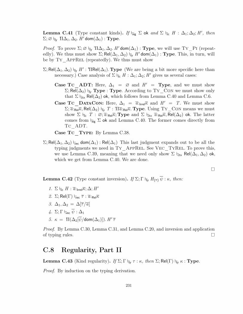
Lemma C.41 (Type constant kinds). If sig Σ ok and Σ tc H : ∆1; ∆2;H′, then

Σ;∅ ty ’Π∆1,∆2.H′ dom(∆1) : Type.

Proof. To prove Σ;∅ ty ’Π∆1,∆2.H′ dom(∆1) : Type, we will use Ty_Pi (repeat-

edly). We thus must show Σ; Rel(∆1,∆2) ty H′ dom(∆1) : Type. This, in turn, will

be by Ty_AppRel (repeatedly). We thus must show

Σ; Rel(∆1,∆2) ty H′ : ’ΠRel(∆1).Type (We are being a bit more specific here than

necessary.) Case analysis of Σ tc H : ∆1; ∆2;H ′ gives us several cases:

Case Tc_ADT: Here, ∆1 = ∅ and H ′ = Type, and we must showΣ; Rel(∆2) ty Type : Type. According to Ty_Con we must show onlythat Σ ctx Rel(∆2) ok, which follows from Lemma C.40 and Lemma C.6.

Case Tc_DataCon: Here, ∆1 = a:Irrelκ and H ′ = T . We must showΣ; a:Relκ,Rel(∆2) ty T : ’Πa:Relκ.Type. Using Ty_Con means we mustshow Σ tc T : ∅; a:Relκ; Type and Σ ctx a:Relκ,Rel(∆2) ok. The lattercomes from sig Σ ok and Lemma C.40. The former comes directly fromTc_ADT.

Case Tc_Type: By Lemma C.38.

Σ; Rel(∆1,∆2) vec dom(∆1) : Rel(∆1) This last judgment expands out to be all thetyping judgments we need in Ty_AppRel. See Vec_TyRel. To prove this,we use Lemma C.39, meaning that we need only show Σ ctx Rel(∆1,∆2) ok,which we get from Lemma C.40. We are done.

Lemma C.42 (Type constant inversion). If Σ; Γ ty Hτ ψ : κ, then:

1. Σ tc H : a:Irrelκ; ∆;H ′

2. Σ; Rel(Γ) vec τ : a:Relκ

3. ∆1,∆2 = ∆[τ/a]

4. Σ; Γ vec ψ : ∆1

5. κ = ’Π(∆2[ψ/dom(∆1)]).H ′ τ

Proof. By Lemma C.30, Lemma C.31, and Lemma C.20, and inversion and applicationof typing rules.

C.8 Regularity, Part IILemma C.43 (Kind regularity). If Σ; Γ ty τ : κ, then Σ; Rel(Γ) ty κ : Type.

Proof. By induction on the typing derivation.

231

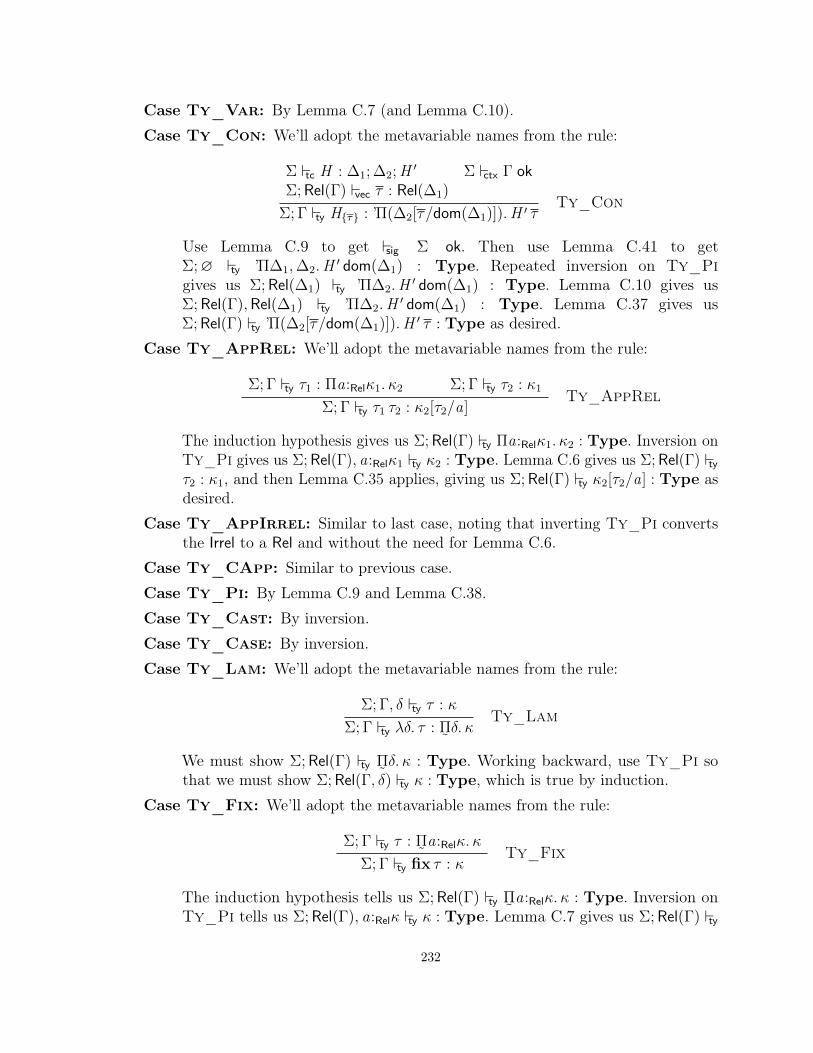
Case Ty_Var: By Lemma C.7 (and Lemma C.10).

Case Ty_Con: We’ll adopt the metavariable names from the rule:

Σ tc H : ∆1; ∆2;H ′ Σ ctx Γ okΣ; Rel(Γ) vec τ : Rel(∆1)

Σ; Γ ty Hτ : ’Π(∆2[τ/dom(∆1)]).H ′ τTy_Con

Use Lemma C.9 to get sig Σ ok. Then use Lemma C.41 to getΣ;∅ ty ’Π∆1,∆2.H

′ dom(∆1) : Type. Repeated inversion on Ty_Pigives us Σ; Rel(∆1) ty ’Π∆2.H

′ dom(∆1) : Type. Lemma C.10 gives usΣ; Rel(Γ),Rel(∆1) ty ’Π∆2.H

′ dom(∆1) : Type. Lemma C.37 gives usΣ; Rel(Γ) ty ’Π(∆2[τ/dom(∆1)]).H ′ τ : Type as desired.

Case Ty_AppRel: We’ll adopt the metavariable names from the rule:

Σ; Γ ty τ1 : Πa:Relκ1. κ2 Σ; Γ ty τ2 : κ1

Σ; Γ ty τ1 τ2 : κ2[τ2/a]Ty_AppRel

The induction hypothesis gives us Σ; Rel(Γ) ty Πa:Relκ1. κ2 : Type. Inversion onTy_Pi gives us Σ; Rel(Γ), a:Relκ1 ty κ2 : Type. Lemma C.6 gives us Σ; Rel(Γ) ty

τ2 : κ1, and then Lemma C.35 applies, giving us Σ; Rel(Γ) ty κ2[τ2/a] : Type asdesired.

Case Ty_AppIrrel: Similar to last case, noting that inverting Ty_Pi convertsthe Irrel to a Rel and without the need for Lemma C.6.

Case Ty_CApp: Similar to previous case.

Case Ty_Pi: By Lemma C.9 and Lemma C.38.

Case Ty_Cast: By inversion.

Case Ty_Case: By inversion.

Case Ty_Lam: We’ll adopt the metavariable names from the rule:

Σ; Γ, δ ty τ : κ

Σ; Γ ty λδ. τ :˜Πδ. κ

Ty_Lam

We must show Σ; Rel(Γ) ty˜Πδ. κ : Type. Working backward, use Ty_Pi so

that we must show Σ; Rel(Γ, δ) ty κ : Type, which is true by induction.

Case Ty_Fix: We’ll adopt the metavariable names from the rule:

Σ; Γ ty τ :˜Πa:Relκ. κ

Σ; Γ ty fix τ : κTy_Fix

The induction hypothesis tells us Σ; Rel(Γ) ty˜Πa:Relκ. κ : Type. Inversion on

Ty_Pi tells us Σ; Rel(Γ), a:Relκ ty κ : Type. Lemma C.7 gives us Σ; Rel(Γ) ty

232

κ : Type as desired.Case Ty_Absurd: Immediate.

Lemma C.44 (Proposition regularity). If Σ; Γ co γ : φ, then Σ; Rel(Γ) prop φ ok.

Proof. By induction on the typing derivation.

Case Co_Var: By Lemma C.8, Lemma C.9, and Lemma C.10.Case Co_Refl: Immediate.Case Co_Sym: By induction.Case Co_Trans: By induction.Case Co_Coherence: Immediate.Case Co_Con: Immediate.Case Co_AppRel: Immediate.Case Co_AppIrrel: Immediate.Case Co_CApp: Immediate.Case Co_PiTy: We adopt the metavariable names from the statement of the rule:

Σ; Γ co η : κ1Type∼Type κ2

Σ; Γ, a:Relκ1 co γ : σ1Type∼Type σ2

Σ; Γ co Πa:ρη. γ : (Πa:ρκ1. σ1) Type∼Type (Πa:ρκ2. (σ2[a B sym η/a]))Co_PiTy

The induction hypothesis (and inversion) give us the following:

• Σ; Rel(Γ) ty κ1 : Type

• Σ; Rel(Γ) ty κ2 : Type

• Σ; Rel(Γ), a:Relκ1 ty σ1 : Type

• Σ; Rel(Γ), a:Relκ1 ty σ2 : Type

We can straightforwardly use Ty_Pi to show that Σ; Rel(Γ) ty Πa:ρκ1. σ1 :Type. Choose a fresh b. We know Σ ctx Rel(Γ), a:Relκ1 ok by Lemma C.9.We can then use Ctx_TyVar (with Lemma C.6) to show that Σ ctx

Rel(Γ), b:Relκ2, a:Relκ1 ok (along with a little inversion and rebuilding to re-order the variables). We established above that Σ; Rel(Γ), a:Relκ1 ty σ2 :Type. Use weakening, Lemma C.10, (here and elsewhere in this case) toget Σ; Rel(Γ), b:Relκ2, a:Relκ1 ty σ2 : Type. We can use Co_Sym to seethat Σ; Rel(Γ), b:Relκ2 co sym η : κ2 ∼ κ1 and then Ty_Cast to see thatΣ; Rel(Γ), b:Relκ2 ty bBsym η : κ1. Lemma C.35 then gives us Σ; Rel(Γ), b:Relκ2 ty

σ2[b B sym η/a] : Type. Use Ty_Pi to get Σ; Rel(Γ) ty Πb:ρκ2. (σ2[b Bsym η/a]) : Type and α-equivalence to get Σ; Rel(Γ) ty Πa:ρκ2. (σ2[a Bsym η/a]) : Type. We are done by Prop_Equality.

233

Case Co_PiCo: We adopt the metavariable names from the statement of the rule:

Σ; Γ co η1 : τ1κ3∼κ4 τ2 Σ; Γ co η2 : σ1

κ5∼κ6 σ2

Σ; Γ, c:τ1κ3∼κ5 σ1 co γ : κ1

Type∼Type κ2 c # γη3 = η1 # c # sym η2

Σ; Γ co Πc:(η1, η2). γ : (Πc:τ1 κ3∼κ5 σ1. κ1) Type∼Type (Πc:τ2 κ4∼κ6 σ2. (κ2[η3/c]))Co_PiCo

The induction hypothesis (and inversion) give us the following:

• Σ; Rel(Γ) ty τ1 : κ3

• Σ; Rel(Γ) ty τ2 : κ4

• Σ; Rel(Γ) ty σ1 : κ5

• Σ; Rel(Γ) ty σ2 : κ6

• Σ; Rel(Γ), c:τ1 ∼ σ1 ty κ1 : Type

• Σ; Rel(Γ), c:τ1 ∼ σ1 ty κ2 : Type

We can straightforwardly use Ty_Pi to show that Σ; Rel(Γ) ty Πc:τ1 ∼ σ1. κ1 :Type. Choose a fresh b. We know Σ ctx Rel(Γ), c:τ1 ∼ σ1 ok by LemmaC.9. We can then use Ctx_CoVar (with Lemma C.6) to show that Σ ctx

Rel(Γ), c2:τ2 ∼ σ2, c:τ1 ∼ σ1 ok (along with a little inversion and rebuilding toreorder the variables). We also know Σ; Rel(Γ), c:τ1 ∼ σ1 ty κ2 : Type. Useweakening, Lemma C.10, (here and elsewhere in this case) to get Σ; Rel(Γ), c2:τ2 ∼σ2, c:τ1 ∼ σ1 ty κ2 : Type. We can use typing rules straightforwardly to seethat Σ; Rel(Γ), c2:τ2 ∼ σ2 co η1 # c2 # sym η2 : τ1 ∼ σ1. Lemma C.36 then givesus Σ; Rel(Γ), c2:τ2 ∼ σ2 ty κ2[η1 # c2 # sym η2/c] : Type. Use Ty_Pi to getΣ; Rel(Γ) ty Πc2:τ2 ∼ σ2. (κ2[η1 # c2 # sym η2/c]) : Type and α-equivalence toget Σ; Rel(Γ) ty Πc:τ2 ∼ σ2. (κ2[η1 # c # sym η2/c]) : Type. We are done.

Case Co_Case: Immediate.Case Co_Lam: We adopt the metavariable names from the statement of the rule:

Σ; Γ co η : κ1Type∼Type κ2

Σ; Γ, a:ρκ1 co γ : τ1σ1∼σ2 τ2

Σ; Γ, a:ρκ1 ty τ1 : σ1 Σ; Γ, a:ρκ1 ty τ2 : σ2

Σ; Γ co λa:ρη. γ : λa:ρκ1. τ1 ˜Πa:ρκ1. σ1∼˜

Πa:ρκ2. (σ2[aBsym η/a]) λa:ρκ2. (τ2[a B sym η/a])Co_Lam

We can use Ty_Lam to get Σ; Γ ty λa:ρκ1. τ1 :˜Πa:ρκ1. σ1. Proceeding similarly

to the case for Co_PiTy, we can get Σ; Γ ty λa:ρκ2. (τ2[a B sym η/a]) :

˜Πa:ρκ2. (σ2[a B sym η/a]) and we are done by Lemma C.6.

Case Co_CLam: Similar to previous case and the case for Co_PiCo.

Case Co_Fix: Immediate.

Case Co_Absurd: By induction and Ty_Absurd.

Case Co_ArgK: By induction, inversion, Lemma C.9, and Lemma C.7.

Case Co_CArgK1: By induction, inversion, Lemma C.9, and Lemma C.8.

234

Case Co_CArgK2: Similar to previous case.

Case Co_ArgKLam: Similar to case for Co_ArgK.

Case Co_CArgKLam1: Similar to case for Co_CArgK1.

Case Co_CArgKLam2: Similar to previous case.

Case Co_Res: Immediate.

Case Co_ResLam: Immediate.

Case Co_InstRel: We adopt the metavariable names from the statement of therule:

Σ; Γ co γ : Πa:Relκ1. σ1 ∼ Πa:Relκ2. σ2

Σ; Γ co η : τ1κ1∼κ2 τ2

Σ; Γ co γ@η : σ1[τ1/a] ∼ σ2[τ2/a]Co_InstRel

We will prove that σ1[τ1/a] is well-typed; the proof for σ2[τ2/a] is similar. Theinduction hypothesis (and some inversion) tells us Σ; Rel(Γ) ty Πa:Relκ1. σ1 :Type. Further inversion gives us Σ; Γ, a:Relκ1 ty σ1 : Type. The inductionhypothesis and an inversion also gives us Σ; Rel(Γ) ty τ1 : κ1. Lemma C.35 givesus Σ; Rel(Γ) ty σ1[τ1/a] : Type as desired.

Case Co_InstIrrel: Similar to previous case.

Case Co_CInst: Similar to previous case.

Case Co_InstLamRel: Similar to previous case.

Case Co_InstLamIrrel: Similar to previous case.

Case Co_CInstLam: Similar to previous case.

Case Co_NthRel: Immediate.

Case Co_NthIrrel: Immediate.

Case Co_Left: Immediate.Case Co_RightRel: We adopt the metavariable names from the statement of

the rule:

Σ; Γ co γ : τ1 σ1κ3[σ1/a]∼κ4[σ2/a] τ2 σ2

Σ; Γ ty σ1 : κ1 Σ; Γ ty σ2 : κ2 Σ; Γ co η : κ1Type∼Type κ2

Σ; Γ co rightη γ : σ1κ1∼κ2 σ2

Co_RightRel

The induction hypothesis tells us Σ; Rel(Γ) prop τ1 σ1κ3[σ1/a]∼κ4[σ2/a] τ2 σ2 ok,

and thus inversion gives us Σ; Rel(Γ) ty τ1 σ1 : κ3[σ1/a]. We know Σ; Γ ty τ1 :’Πa:Relκ1. κ3, and thus we can invert the type application to get Σ; Rel(Γ) ty σ1 :κ1 as desired. We can similarly derive the type for σ2, and we are thus done.

Case Co_RightIrrel: Similar to previous case.

Case Co_Kind: By Lemma C.43.

Case Co_Step: Immediate.

235

C.9 PreservationLemma C.45 (Correctness of build_kpush_co). Assume Σ; Γ cev ψ : ∆[τ/a], and letγi = build_kpush_co(η;ψ1...i−1) and ψ′i = cast_kpush_arg(ψi ; γi). If Σ; Rel(Γ) co η :(’Π∆. σ)[τ/a] ∼ (’Π∆. σ)[τ ′/a], then:

1. Σ; Rel(Γ) co build_kpush_co(η;ψ) : σ[τ/a][ψ/dom(∆)] ∼ σ[τ ′/a][ψ′/dom(∆)]

2. Σ; Γ cev ψ′: ∆[τ ′/a]

Proof. Proceed by induction on Σ; Γ cev ψ : ∆[τ/a].

Case Cev_Nil: In this case, both ψ and ∆ are empty. We must proveΣ; Rel(Γ) co build_kpush_co(η;∅) : σ[τ/a] ∼ σ[τ ′/a]. By definition,build_kpush_co(η;∅) = η. We are done by assumption and Cev_Nil.

Case Cev_TyRel: In this case, we have ψ = ψ0, τ0 and ∆ = ∆0, b:Relκ withΣ; Γ cev ψ0 : ∆0[τ/a] and Σ; Γ ty τ0 : κ[τ/a][ψ0/dom(∆0)]. We can see thatbuild_kpush_co(η;ψ0, τ0) = let c := build_kpush_co(η;ψ0) in c@(τ0 ≈argk c

τ0 B argk c). The induction hypothesis tells us that Σ; Rel(Γ) co c :

(’Πb:Relκ. σ)[τ/a][ψ0/dom(∆0)] ∼ (’Πb:Relκ. σ)[τ ′/a][ψ′0/dom(∆0)]. We can thus

deduce the following:

• Σ; Rel(Γ) co argk c : κ[τ/a][ψ0/dom(∆0)] ∼ κ[τ ′/a][ψ′0/dom(∆0)]

• Σ; Rel(Γ) ty τ0 B argk c : κ[τ ′/a][ψ′0/dom(∆0)]

• Σ; Rel(Γ) co τ0 ≈argk c τ0 B argk c : τ0 ∼ τ0 B argk c

• Σ; Rel(Γ) co c@(τ0 ≈argk c τ0 B argk c) : σ[τ/a][ψ0/dom(∆0)][τ0/b] ∼σ[τ ′/a][ψ

′0/dom(∆0)][τ0 B argk c/b]

Note that cast_kpush_arg(τ0; c) = τ0 B argk c and thus that we can sayτ ′0 = τ0 B argk c. Noting that the ψ0 cannot have b free due to the Barendregtconvention, we can rewrite the substutition [ψ0/dom(∆0)][τ0/b] as [ψ/dom(∆)]and rewrite the last judgment above as Σ; Rel(Γ) co build_kpush_co(η;ψ) :

σ[τ/a][ψ/dom(∆)] ∼ σ[τ ′/a][ψ′/dom(∆)], which is what we are trying to prove.

We are done proving result (1).

For result (2), we must prove Σ; Γ cev ψ′0, τ0 B argk c : ∆0[τ

′/a], b:Relκ[τ ′/a].This fact comes from a straightforward use of Cev_TyRel.

Case Cev_TyIrrel: Similar to previous case.

Case Cev_Co: In this case, we have ψ = ψ0, γ0 and ∆ =∆0, c0:φ0 with Σ; Γ cev ψ0 : ∆0[τ/a] and Σ; Rel(Γ) co γ0 :φ0[τ/a][ψ0/dom(∆0)]. We can see that build_kpush_co(η;ψ0, γ0) = let c :=

236

build_kpush_co(η;ψ0) in c@(γ0, sym (argk1 c) # γ0 # argk2 c). The inductionhypothesis tells us that Σ; Rel(Γ) co c : (’Πc0:φ0. σ)[τ/a][ψ0/dom(∆0)] ∼(’Πc0:φ0. σ)[τ ′/a][ψ

′0/dom(∆0)]. Let φ0 = σ1 ∼ σ2. We can thus deduce the

following:

• Σ; Rel(Γ) co sym (argk1 c) : σ1[τ′/a][ψ

′0/dom(∆0)] ∼

σ1[τ/a][ψ0/dom(∆0)]

• Σ; Rel(Γ) co argk2 c : σ2[τ/a][ψ0/dom(∆0)] ∼ σ2[τ ′/a][ψ′0/dom(∆0)]

• Σ; Rel(Γ) co sym (argk1 c) # γ0 # argk2 c : σ1[τ′/a][ψ

′0/dom(∆0)] ∼

σ2[τ ′/a][ψ′0/dom(∆0)]

• Σ; Rel(Γ) co c@(γ0, sym (argk1 c) # γ0 # argk2 c) :

σ[τ/a][ψ0/dom(∆0)][γ0/c0] ∼ σ[τ ′/a][ψ′0/dom(∆0)][sym (argk1 c) #

γ0 # argk2 c/c0]

Note that cast_kpush_arg(γ0; c) = sym (argk1 c) # γ0 # argk2 c and thus thatwe can say γ′0 = sym (argk1 c) # γ0 # argk2 c. Noting that the ψ0 cannothave c0 free due to the Barendregt convention, we can rewrite the substitution[ψ0/dom(∆0)][γ0/c0] as [ψ/dom(∆)] and rewrite the last judgment above asΣ; Rel(Γ) co build_kpush_co(η;ψ) : σ[τ/a][ψ/dom(∆)] ∼ σ[τ ′/a][ψ

′/dom(∆)],

which is what we are trying to prove. We are done proving result (1).

To prove result (2), we must show Σ; Γ cev ψ′0, sym (argk1 c) # γ0 # argk2 c :

∆0[τ ′/a], c0:φ0[τ ′/a], which we get from a straightforward use of Cev_Co.

Remark. Lemma C.45 could also be rewritten to work with˜Π, but with no need.

Theorem C.46 (Preservation). If Σ; Γ ty τ : κ and Σ; Γ s τ −→ τ ′, then Σ; Γ ty τ′ :

κ.

Proof. By induction on the typing derivation.

Case Ty_Var: Impossible, as variables do not step.

Case Ty_Con: Impossible, as constants do not step.

Case Ty_AppRel: We now have several cases, depending on how the expressionhas stepped:

Case S_BetaRel: By Lemma C.35.Case S_App_Cong: By induction.

237

Case S_PushRel: We adopt the metavariable names from the statement ofthe rule:

Σ; Rel(Γ) co γ0 : Πa:Relκ. σ ∼ Πa:Relκ′. σ′

γ1 = sym (argk γ0) γ2 = γ0@(τ B γ1 ≈sym γ1 τ)

Σ; Γ s (v B γ0) τ −→ v (τ B γ1)B γ2

S_PushRel

Inversion on Σ; Γ ty (v B γ0) τ : κ0 gives us Σ; Γ ty τ : κ′ and Σ; Γ ty v :Πa:ρκ. σ. Straightforward application of typing rules gives us Σ; Rel(Γ) co

γ1 : κ′ ∼ κ and Σ; Rel(Γ) co γ2 : σ[τ B γ1/a] ∼ σ′[τ/a]. We can thenderive Σ; Γ ty τ B γ1 : κ and thus Σ; Γ ty v (τ B γ1) : σ[τ B γ1/a] andΣ; Γ ty v (τ B γ1)B γ2 : σ′[τ/a] as desired.

Case Ty_AppIrrel: We now have several cases:

Case S_BetaIrrel: By Lemma C.35.Case S_App_Cong: By induction.Case S_PushIrrel: Similar to the case for S_PushRel.

Case Ty_CApp: We now have several cases:

Case S_CBeta: By Lemma C.36.Case S_App_Cong: By induction.Case S_CPush: We adopt the metavariable names of the rule:

Σ; Rel(Γ) co γ0 : Πc:φ. σ ∼ Πc:φ′. σ′

γ1 = argk1 γ0 γ2 = argk2 γ0

η′ = γ1 # η # sym γ2 γ3 = γ0@(η′, η)

Σ; Γ s (v B γ0) η −→ v η′ B γ3

S_CPush

We can see that Σ; Γ ty (v B γ0) η : σ′[η/c]. Let φ = τ1 ∼ τ2 andφ′ = τ3 ∼ τ4. Inversion and application of typing rules tells us the following:• Σ; Γ ty v : Πc:φ. σ• Σ; Rel(Γ) co η : τ3 ∼ τ4

• Σ; Rel(Γ) co γ1 : τ1 ∼ τ3

• Σ; Rel(Γ) co γ2 : τ2 ∼ τ4

• Σ; Rel(Γ) co η′ : τ1 ∼ τ2

• Σ; Rel(Γ) co γ3 : σ[η′/c] ∼ σ′[η/c]• Σ; Γ ty v η

′ : σ[η′/c]• Σ; Γ ty v η

′ B γ3 : σ′[η/c]

Note that the last fact proves this case.

Case Ty_Pi: Impossible, as Π-types do not step.

Case Ty_Cast: We now have several cases:

238

Case S_Trans: We adopt the metavariable names of the rule:

Σ; Γ s (v B γ1)B γ2 −→ v B (γ1 # γ2)S_Trans

We know Σ; Γ ty (v B γ1)B γ2 : κ. Inversion and typing rules give us thefollowing:

• Σ; Rel(Γ) co γ2 : κ2 ∼ κ• Σ; Rel(Γ) co γ1 : κ3 ∼ κ2

• Σ; Γ ty v : κ3

• Σ; Rel(Γ) co γ1 # γ2 : κ3 ∼ κ• Σ; Γ ty v B (γ1 # γ2) : κ

Note that the last fact proves this case.Case S_Cast_Cong: By induction.

Case Ty_Case: We now have several cases:

Case S_Match: We adopt the metavariable names of the rule:

alti = H → τ0

Σ; Γ s caseκHτ ψ of alt −→ τ0 ψ 〈Hτ ψ〉S_Match

Inversion and typing rules tell us the following:

• Σ; Γ ty Hτ ψ : ’Π∆′.H ′ σ (premise of Ty_Case)• Using Lemma C.42:

– Σ tc H : a:Irrelκ; ∆2;H ′

– ∆0,∆1 = ∆2[τ/a]– Σ; Γ vec ψ : ∆0

– ∆′ = ∆1[ψ/dom(∆0)] and σ = τ (Lemma C.20)• The premises of Alt_Match (also using Lemma C.18):

– ∆3,∆4 = ∆2[τ/a]– |∆4| = |∆1|– Σ; Γ ty τ0 : ?Π∆3, c:Hτ ψ ∼ Hτ dom(∆3). κ

• ∆3 = ∆0 and ∆4 = ∆1 (from |∆4| = |∆1| and the definitions of ∆0,∆1, ∆3, and ∆4)• Σ; Γ ty τ0 : ?Π∆0, c:Hτ ψ ∼ Hτ dom(∆0). κ (rewriting)• Σ; Γ ty τ0 ψ : ?Πc:Hτ ψ ∼ Hτ ψ. κ (Lemma C.31, where the κ needs

no substitution by Lemma C.12)• Σ; Γ ty τ0 ψ 〈Hτ ψ〉 : κ (Co_Refl and Ty_CApp, where the κ

needs no substitution by Lemma C.12)

Note that this last fact proves this case.

239

Case S_Default: We adopt the metavariable names of the rule:

alti = _→ σ no alternative in alt matches HΣ; Γ s caseκHτ ψ of alt −→ σ

S_Default

By Ty_Case, the redex has kind κ; inversion also gives us Σ; Γ; σ0 `τalt_→ σ : κ. Inverting Alt_Default gives us our goal.

Case S_DefaultCo: Similar to previous case.Case S_Case_Cong: By induction.Case S_KPush: We adopt the metavariable names of the rule:

Σ tc H : a:Irrelκ; ∆;H ′ ∆ = ∆1,∆2 n = |∆2|κ = ’Πa:Irrelκ,∆.H

′ a

σ = ’Π(∆2[τ/a][ψ/dom(∆1)]).H ′ τ

σ′ = ’Π(∆2[τ ′/a][ψ′/dom(∆1)]).H ′ τ ′

Σ; Rel(Γ) co η : σ ∼ σ′

Σ; Rel(Γ) vec τ′ : a:Relκ

∀i , γi = build_kpush_co(〈κ〉@(nths (resn η));ψ1...i−1)∀i , ψ′i = cast_kpush_arg(ψi ; γi)

H → κ′ ∈ alt

Σ; Γ s caseκ0 (Hτ ψ)B η of alt −→ caseκ0 Hτ ′ ψ′of alt

S_KPush

Note that we need to prove only that the type of (Hτ ψ)B η matches thatof Hτ ′ ψ

′, namely ’Π(∆2[τ′/a][ψ

′/dom(∆1)]).H

′ τ ′. We can derive thesefacts:• Σ; Γ ty Hτ ψ : ’Π(∆2[τ/a][ψ/dom(∆1)]).H

′ τ (by inversion of thetyping judgment on the redex)• Σ; Γ ty Hτ : ’Π(∆1[τ/a],∆2[τ/a]).H ′ τ (by Lemma C.30 followed by

inverting Ty_Con)• Σ; Γ vec ψ : ∆1[τ/a] (also from Lemma C.30)• Σ; Γ vec τ : a:Relκ (by inversion)• Σ; Rel(Γ) vec τ

′ : a:Relκ (from S_KPush)• Σ; Rel(Γ) co resn η : H ′ τ ∼ H ′ τ ′ (with the well-formedness of τ andτ ′ telling us that the τ and τ ′ do not have any variables in dom(∆2)free)• ∀i ,∃κi , Σ; Rel(Γ) ty τi : κi (by Lemma C.29)• ∀i ,∃κ′i , Σ; Rel(Γ) ty τ

′i : κ′i (by Lemma C.29)

• ∀i , Σ; Rel(Γ) co nthi (resn η) : τi ∼ τ ′i (from Co_NthRel)• Σ; Γ ty κ : Type, recalling that κ = ’Πa:Irrelκ,∆.H

′ a (by Lemma C.9,Lemma C.41, and Lemma C.10)• Σ; Γ co 〈κ〉 : κ ∼ κ (by Co_Refl)• Σ; Γ co 〈κ〉@(nths (resn η)) : (’Π∆1,∆2.H

′ a)[τ/a] ∼

240

(’Π∆1,∆2.H′ a)[τ ′/a] (by Lemma C.32)

• Σ; Γ cev ψ : ∆1[τ/a] (by Lemma C.27)• Σ; Γ cev ψ

′: ∆1[τ ′/a] (by Lemma C.45)

• Σ; Γ vec ψ′: ∆1[τ ′/a] (by Lemma C.27)

• Σ; Γ ty Hτ ′ : ’Π(∆1[τ′/a],∆2[τ

′/a]).H ′ τ ′ (by a use of Ty_Con,along with Lemma C.9)• Σ; Γ ty Hτ ′ ψ

′: ’Π(∆2[τ ′/a][ψ

′/dom(∆1)]).H ′ τ ′

This last fact is what we are trying to prove, and so we are done.

Case Ty_Lam: We now have several cases:

Case S_IrrelAbs_Cong: By induction.Case S_APush: We adopt the metavariable names from the rule:

γ1 =˜Πa:Irrel〈κ〉. γ γ2 = τ1 ≈〈Type〉 τ2

τ1 =˜Πa:Irrelκ. (κ1[a B sym 〈κ〉/a]) τ2 =

˜Πa:Irrelκ. κ1

Σ; Γ s λa:Irrelκ. (v B γ) −→ (λa:Irrelκ. v)B (γ1 # γ2)S_APush

Inversion and typing rules then give us the following facts:

• Σ; Γ ty λa:Irrelκ. (v B γ) :˜Πa:Irrelκ. κ1

• Σ; Γ, a:Irrelκ ty v B γ : κ1

• Σ; Rel(Γ), a:Relκ co γ : κ0 ∼ κ1

• Σ; Γ, a:Irrelκ ty v : κ0

• Σ; Γ ty λa:Irrelκ. v :˜Πa:Irrelκ. κ0

• Σ; Rel(Γ) ty κ : Type (by Lemma C.9 and Lemma C.7)• Σ; Rel(Γ) co 〈κ〉 : κ ∼ κ (by Co_Refl)• Σ; Rel(Γ) co

˜Πa:Irrel〈κ〉. γ :

˜Πa:Irrelκ. κ0 ∼

˜Πa:Irrelκ. (κ1[a B sym 〈κ〉/a])

(by Co_PiTy)• Σ; Rel(Γ) ty

˜Πa:Irrelκ. (κ1[a B sym 〈κ〉/a]) : Type (by Lemma C.44)

• Σ; Rel(Γ) ty˜Πa:Irrelκ. κ1 : Type (by Lemma C.43)

• Σ; Rel(Γ) co (˜Πa:Irrelκ. (κ1[a B sym 〈κ〉/a])) ≈〈Type〉 (

˜Πa:Irrelκ. κ1) :

(˜Πa:Irrelκ. (κ1[a B sym 〈κ〉/a])) ∼ (

˜Πa:Irrelκ. κ1) (by Co_Coherence)

We can then conclude, by Co_Trans and Ty_Cast, that the result hasthe same type,

˜Πa:Irrelκ. κ1 as the redex.

Case Ty_Fix: We now have several cases:

Case S_Unroll: We adopt the variable names from the rule:

τ = λa:Relκ. σ

Σ; Γ s fix τ −→ σ[fix τ/a]S_Unroll

We can then derive the following:

241

• Σ; Γ ty λa:Relκ. σ :˜Πa:Relκ. κ (by inversion)

• Σ; Γ, a:Relκ ty σ : κ (by inversion)• Σ; Γ ty fix (λa:Relκ. σ) : κ (by Ty_Fix)• Σ; Γ ty σ[fix (λa:Relκ. σ)/a] : κ (by Lemma C.35)

This last judgment is what we are trying to prove; we are done.Case S_Fix_Cong: By induction.Case S_FPush: We adopt the metavariable names from the rule:

γ1 = γ0@(a ≈γ2 a B γ2) # sym γ2

γ2 = argk γ0

Σ; Γ s fix ((λa:Relκ. σ)B γ0) −→ (fix (λa:Relκ. (σ B γ1)))B γ2

S_FPush

We can derive the following facts:• Σ; Γ ty fix ((λa:Relκ. σ)B γ0) : κ1 (conclusion of Ty_Fix)• Σ; Γ ty (λa:Relκ. σ)B γ0 :

˜Πa:Relκ1. κ1 (premise of Ty_Fix)

• Σ; Rel(Γ) co γ0 : κ0 ∼˜Πa:Relκ1. κ1 (inversion on Ty_Cast)

• Σ; Γ ty λa:Relκ. σ : κ0 (same inversion)• Σ; Γ ty λa:Relκ. σ :

˜Πa:Relκ. κ2 (inversion by Ty_Lam)

• κ0 =˜Πa:Relκ. κ2 (Lemma C.20)

• Σ; Γ, a:Relκ ty σ : κ2 (inversion by Ty_Lam)• Σ; Rel(Γ) co γ0 : (

˜Πa:Relκ. κ2) ∼ (

˜Πa:Relκ1. κ1) (substitution)

• Σ; Rel(Γ) co argk γ0 : κ ∼ κ1 (Co_ArgK)• γ2 = argk γ0 (premise of S_FPush)• Σ; Γ, a:Relκ ty a B γ2 : κ1 (Ty_Cast)• Σ; Γ, a:Relκ co a ≈γ2 a B γ2 : a ∼ a B γ2 (Co_Coherence)• Σ; Γ, a:Relκ co γ0@(a ≈γ2 a B γ2) : κ2 ∼ κ1[a B γ2/a] (Co_InstRel)• Σ; Rel(Γ) ty

˜Πa:Relκ1. κ1 : Type (Lemma C.43)

• Σ; Rel(Γ), a:Relκ1 ty κ1 : Type (inversion on Ty_Pi)• Σ; Rel(Γ) ty κ1 : Type (Lemma C.7 and Lemma C.10)• κ1[a B γ2/a] = κ1 (Lemma C.12, noting that a # κ1)• Σ; Γ, a:Relκ co γ0@(a ≈γ2 a B γ2) : κ2 ∼ κ1 (substitution)• Σ; Γ, a:Relκ co sym γ2 : κ1 ∼ κ (Co_Sym with Lemma C.10)• γ1 = γ0@(a ≈γ2 a B γ2) # sym γ2 (premise of S_FPush)• Σ; Γ, a:Relκ co γ1 : κ2 ∼ κ (Co_Trans)• Σ; Γ, a:Relκ ty σ B γ1 : κ (Ty_Cast and Lemma C.6)• Σ; Γ ty λa:Relκ. (σ B γ1) :

˜Πa:Relκ. κ (Ty_Lam)

• Σ; Γ ty fix (λa:Relκ. (σ B γ1)) : κ (Ty_Fix)• Σ; Γ ty (fix (λa:Relκ. (σ B γ1)))B γ2 : κ1 (Ty_Cast)

The last item proves this case.

Case Ty_Absurd: Impossible, as absurd γ τ does not step.

242

C.10 ConsistencyDefinition C.47 (Coercion erasure). Define the erasure of a type ε = bτc by thefollowing function (including auxiliary functions):

bac = a

bHτc = Hbτc

bτ1 τ2c = bτ1c bτ2cbτ1 τ2c = bτ1c bτ2cbτ γc = bτc •bΠδ. τc = Πbδc. bτcbτ B γc = bτc

bcaseκ τ of altc = casebκc bτcof baltcbλδ. τc = λbδc. bτcbfix τc = fix bτc

babsurd γ τc = absurd • bτc

ba:ρκc = a:ρbκcbc:φc = •:bφc

bτ1κ1∼κ2 τ2c = bτ1c bκ1c∼bκ2c bτ2c

bπ → τc = π → bτc

Notation C.48 (Erased types in consistency proof). The rewrite relation is definedonly over erased types. We use a convention that the occurrence of a metavariablein a mention of the relation indicates that the metavariable represents an erasedelement.

Notation C.49 (Reduction).

• We write ψ ψ′ to mean ∀i , ψi ψ′i .

• We write τ1 τ3 τ2 to mean τ1 τ3 and τ2 τ3.

• We write ∗ to mean the reflexive, transitive closure of .

• We write τ1 ∗ τ3∗ τ2 to mean τ1 ∗ τ3 and τ2 ∗ τ3.

Lemma C.50 (Parallel reduction substitution). Assume ψ ψ′. We can then

conclude:

1. τ [ψ/z ] τ [ψ′/z ]

2. δ[ψ/z ] δ[ψ′/z ]

243

Proof. By straightforward mutual induction on the structure of τ/δ.

Lemma C.51 (Parallel reduction substitution in parallel). Assume ψ ψ′.

1. If τ1 τ2, then τ1[ψ/z ] τ2[ψ′/z ].

2. If δ1 δ2, then δ1[ψ/z ] δ2[ψ′/z ].

Proof. By induction on τ1 τ2/δ1 δ2.

Case R_Refl: By Lemma C.50.

Congruence rules: By induction.

Case R_BetaRel: It must be that τ1 = (λb:Relκ1. τ3) τ4 and τ2 = τ ′3[τ ′4/b] whereτ3 τ ′3 and τ4 τ ′4. We must show that (λb:Relκ1[ψ/z ]. τ3[ψ/z ]) τ4[ψ/z ] τ ′3[τ ′4/b][ψ

′/z ]. Proceeding by R_BetaRel, the left-hand-side steps to τ5[τ6/b]

where τ3[ψ/z ] τ5 and τ4[ψ/z ] τ6. (We can choose τ5 and τ6.) We mustthus show that τ5[τ6/b] = τ ′3[τ ′4/b][ψ

′/z ]. First, we reorder substitutions to get

τ ′3[τ′4/b][ψ

′/z ] = τ ′3[ψ

′/z ][τ ′4[ψ

′/z ]/b], noting that b # ψ

′ by the Barendregtconvention. Choose τ5 = τ ′3[ψ

′/z ] and τ6 = τ ′4[ψ

′/z ]. We must show that

τ3[ψ/z ] τ5 and τ4[ψ/z ] τ6; expanding gives us that we must show τ3[ψ/z ] τ ′3[ψ

′/z ] and τ4[ψ/z ] τ ′4[ψ

′/z ]. Both of these follow directly from the induction

hypothesis, and so we are done.

Case R_BetaIrrel: Similar to previous case.

Case R_CBeta: By induction.

Case R_Match: It must be that:

• τ1 = caseκHσ ψ0 of alt

• τ2 = τ4 ψ′0 • where H → τ3 ∈ alt , τ3 τ4, and ψ0 ψ

′0.

We must show that caseκ[ψ/z ] Hσ[ψ/z ] ψ0[ψ/z ] of alt [ψ/z ] τ4[ψ′/z ]ψ

′0[ψ′/z ] •.

Proceeding by R_Match, the left-hand side steps to τ5 ψ′′0 • where τ3[ψ/z ] τ5

and ψ0[ψ/z ] ψ′′0, and we get to choose τ5 and ψ

′′0. We must show that

τ5 ψ′′0 • = τ4[ψ

′/z ]ψ

′0[ψ′/z ] •. Choose τ5 = τ4[ψ

′/z ] and ψ

′′0 = ψ

′0[ψ′/z ]. We

must show that τ3[ψ/z ] τ4[ψ′/z ] and ψ0[ψ/z ] ψ

′0[ψ′/z ]. Both of these follow

from the induction hypothesis, and so we are done.

Case R_Default: It must be that:

• τ1 = caseκHσ ψ0 of _→ σ0; alt

• τ2 = σ′0 where σ0 σ′0

We are done by the induction hypothesis.

Case R_Unroll: It must be that:

244

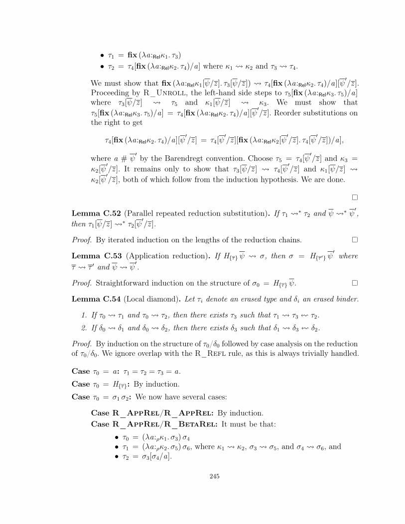
• τ1 = fix (λa:Relκ1. τ3)

• τ2 = τ4[fix (λa:Relκ2. τ4)/a] where κ1 κ2 and τ3 τ4.

We must show that fix (λa:Relκ1[ψ/z ]. τ3[ψ/z ]) τ4[fix (λa:Relκ2. τ4)/a][ψ′/z ].

Proceeding by R_Unroll, the left-hand side steps to τ5[fix (λa:Relκ3. τ5)/a]where τ3[ψ/z ] τ5 and κ1[ψ/z ] κ3. We must show thatτ5[fix (λa:Relκ3. τ5)/a] = τ4[fix (λa:Relκ2. τ4)/a][ψ

′/z ]. Reorder substitutions on

the right to get

τ4[fix (λa:Relκ2. τ4)/a][ψ′/z ] = τ4[ψ

′/z ][fix (λa:Relκ2[ψ

′/z ]. τ4[ψ

′/z ])/a],

where a # ψ′ by the Barendregt convention. Choose τ5 = τ4[ψ

′/z ] and κ3 =

κ2[ψ′/z ]. It remains only to show that τ3[ψ/z ] τ4[ψ

′/z ] and κ1[ψ/z ]

κ2[ψ′/z ], both of which follow from the induction hypothesis. We are done.

Lemma C.52 (Parallel repeated reduction substitution). If τ1 ∗ τ2 and ψ ∗ ψ′,

then τ1[ψ/z ] ∗ τ2[ψ′/z ].

Proof. By iterated induction on the lengths of the reduction chains.

Lemma C.53 (Application reduction). If Hτ ψ σ, then σ = Hτ ′ ψ′where

τ τ ′ and ψ ψ′.

Proof. Straightforward induction on the structure of σ0 = Hτ ψ.

Lemma C.54 (Local diamond). Let τi denote an erased type and δi an erased binder.

1. If τ0 τ1 and τ0 τ2, then there exists τ3 such that τ1 τ3 τ2.

2. If δ0 δ1 and δ0 δ2, then there exists δ3 such that δ1 δ3 δ2.

Proof. By induction on the structure of τ0/δ0 followed by case analysis on the reductionof τ0/δ0. We ignore overlap with the R_Refl rule, as this is always trivially handled.

Case τ0 = a: τ1 = τ2 = τ3 = a.

Case τ0 = Hτ: By induction.

Case τ0 = σ1 σ2: We now have several cases:

Case R_AppRel/R_AppRel: By induction.Case R_AppRel/R_BetaRel: It must be that:

• τ0 = (λa:ρκ1. σ3)σ4

• τ1 = (λa:ρκ2. σ5)σ6, where κ1 κ2, σ3 σ5, and σ4 σ6, and• τ2 = σ3[σ4/a].

245

Choose τ3 = σ5[σ6/a]. We must show τ1 τ3 and τ2 τ3. The first is byR_BetaRel. The second is by Lemma C.51.

Case R_BetaRel/R_BetaRel: It must be that:

• τ0 = (λa:ρκ. σ3)σ4

• τ1 = σ′3[σ′4/a], where σ3 σ′3 and σ4 σ′4• τ2 = σ′′3 [σ′′4/a], where σ3 σ′′3 and σ4 σ′′4 .

Using the induction hypothesis, we can get σ5 and σ6 such that

• σ′3 σ5 σ′′3• σ′4 σ6 σ′′4 .

Choose τ3 = σ5[σ6/a]. We must show σ′3[σ′4/a] σ5[σ6/a] and σ′′3 [σ′′4/a] σ5[σ6/a]. Both of these follow from Lemma C.51.

Case τ0 = σ1 σ2: Similar to τ0 = σ1 σ2.

Case τ0 = σ •: We now have several cases:

Case R_CApp/R_CApp: By induction.Case R_CApp/R_CBeta: It must be that:

• τ0 = (λ•:κ1 ∼ κ2. σ3) •• τ1 = (λ•:κ3 ∼ κ4. σ4) • where κ1 κ3, κ2 κ4, and σ3 σ4.• τ2 = σ5 where σ3 σ5

The induction hypothesis gives us σ6 such that σ4 σ6 σ5. Chooseτ3 = σ6. We must show τ1 τ3 and τ2 τ3. The first is by R_CBeta.The second is immediate.

Case R_CBeta/R_CBeta: By induction.

Case τ0 = Πδ. σ0: By induction and R_Pi.

Case τ0 = caseκ σ0 of alt : We now have several cases:

Case R_Case/R_Case: By induction and R_Case.Case R_Case/R_Match: It must be that:

• τ0 = caseκHσ ψ of H → ε

• τ1 = caseκ′ Hσ′ ψ′of H → ε′ where κ κ′, σ σ′, ψ ψ

′, andε ε′ (appealing to Lemma C.53)• τ2 = ε′′i ψ

′′ •, where Hi = H , εi ε′′i , and ψ ψ′′.

Using the induction hypothesis, we can get ε′′′i such that ε′i ε′′′i ε′′i andψ′′′ such that ψ′ ψ

′′′ ψ′′. Choose τ3 = ε′′′i ψ

′′′ •. We must show bothτ1 τ3 and τ2 τ3. The first is by R_Match. The second is by repeateduse of R_AppRel/R_AppIrrel/R_CApp.

Case R_Case/R_Default: It must be that:

246

• τ0 = caseκHσ ψ of _→ σ0; alt

• τ1 = caseκ′ Hσ′ ψ′of _ → σ′0; alt

′ where κ κ′, σ σ′, ψ ψ′,

σ0 σ′0, and alt alt′

• τ2 = σ′′0 where σ0 σ′′0

The induction hypothesis gives us ε such that σ′0 ε σ′′0 . We can seethat τ1 can step by R_Default (as the type constant H does not change),and thus that τ1 ε τ2. We are done.

Case R_Match/R_Match: It must be that:

• τ0 = caseκHσ ψ of alt• alti = H → κ1

• τ1 = κ′1 ψ′ • where κ1 κ′1 and ψ ψ

′.• τ2 = κ′′1 ψ

′′ • where κ1 κ′′1 and ψ ψ′′.

The induction hypothesis gives us κ′′′1 and ψ′′′ such that:

• κ′1 κ′′′1 κ′′1• ψ′ ψ

′′′ ψ′′

Choose τ3 = κ′′′1 [ψ′′′/z ] and we are done by Lemma C.51.

Case R_Match/R_Default: Impossible, as the premises contradict eachother.

Case R_Default/R_Default: By induction.

Case τ0 = λδ0. σ0: By induction and R_Lam.

Case τ0 = fixσ0: We have several cases:

Case R_Fix/R_Fix: By induction.Case R_Fix/R_Unroll: It must be that:

• τ0 = fix (λa:Relκ1. σ1)• τ1 = fix (λa:Relκ2. σ2) where κ1 κ2 and σ1 σ2

• τ2 = σ3[fix (λa:Relκ3. σ3)/a] where κ1 κ3 and σ1 σ3

The induction hypothesis gives us κ4 and σ4 such that κ2 κ4 κ3

and σ2 σ4 σ3. Choose τ3 = σ4[fix (λa:Relκ4. σ4)/a]. We must showτ1 τ3 and τ2 τ3. The first is by R_Unroll, and the second is byLemma C.51.

Case R_Unroll/R_Unroll: It must be that:

• τ0 = fix (λa:Relκ1. σ1)• τ1 = σ2[fix (λa:Relκ2. σ2)/a] where κ1 κ2 and σ1 σ2

• τ2 = σ3[fix (λa:Relκ3. σ3)/a] where κ1 κ3 and σ1 σ3

The induction hypothesis gives us κ4 and σ4 such that κ2 κ4 κ3 andσ2 σ4 σ3. Choose τ3 = σ4[fix (λa:Relκ4. σ4)/a] and we are done byLemma C.51.

247

Case τ0 = absurd γ σ0: By induction and R_Absurd.

Case δ0 = a:ρκ0: By induction and R_TyBinder.

Case δ0 = •:τ1 ∼ τ1: By induction and R_CoBinder.

Lemma C.55 (Confluence). Let τi denote an erased type. If τ1 ∗ τ2 and τ1 ∗ τ3,then there exists τ4 such that τ2 ∗ τ4

∗ τ3.

Proof. Consequence of Lemma C.54.

Lemma C.56 (Π-reduction). If Πδ. τ σ, then there exist δ′ and τ ′ such thatσ = Πδ′. τ ′, δ δ′, and τ τ ′.

Proof. Case anlysis on Πδ. τ σ.

Lemma C.57 (λ-reduction). If λδ. τ σ, then there exist δ′ and τ ′ such thatσ = λδ′. τ ′, δ δ′, and τ τ ′.

Proof. Case anlysis on λδ. τ σ.

Lemma C.58 (Matchable application reduction). If τ ψ σ, then there exist τ ′ andψ′ such that σ = τ ′ ψ′, τ τ ′, and ψ ψ′.

Proof. Case analysis on τ ψ σ.

Lemma C.59 (Coercion substitution/erasure). bτ [γ/c]c = bτc

Proof. By induction on the structure of τ .

Lemma C.60 (Type constant kinds shape). If Σ; Γ ty Hτ1 ψ1 : κ1 and Σ; Γ ty

Hτ2 ψ2 : κ2 (where the lengths of ψ1 and ψ2 are the same), then there exists a κ suchthat fv(κ) = a ∪ z, κ1 = κ[τ 1/a, ψ1/z ], and κ2 = κ[τ 2/a, ψ2/z ].

Proof. Lemma C.30 tells us that there exist κ3 and κ4 such that Σ; Γ ty Hτ1 :κ3 and Σ; Γ ty Hτ2 : κ4. Inversion (via the only applicable rule, Ty_Con)then tells us that Σ tc H : ∆1; ∆2;H

′, κ3 = ’Π(∆2[τ 1/dom(∆1)]).H′ τ 1,

and κ4 = ’Π(∆2[τ 2/dom(∆1)]).H′ τ 2. Lemma C.30 also tells us that Σ; Γ vec

ψ1 : prefix(∆2[τ 1/dom(∆1)]) and Σ; Γ vec ψ2 : prefix(∆2[τ 2/dom(∆1)]). Let∆3,∆4 = ∆2, where the length of ∆3 matches that of ψ1. Thus LemmaC.31 tells us that κ1 = ’Π(∆4[τ 1/dom(∆1), ψ1/dom(∆3)]).H

′ τ 1 and κ2 =’Π(∆4[τ 2/dom(∆1), ψ2/dom(∆3)]).H

′ τ 2. Thus, we are done, with a = dom(∆1),z = dom(∆2), and κ = ’Π∆4.H

′ a.

Definition C.61 (Joinability). We say that two types τ1 and τ2 are joinable if thereexists an erased type ε such that bτ1c ∗ ε ∗ bτ2c.

248

Lemma C.62 (Completeness of type reduction). If Σ; Γ co γ : τ1κ1∼κ2 τ2 and

c # γ for every c:φ ∈ Γ, then:

1. There exists some erased type ε such that bτ1c ∗ ε ∗ bτ2c.2. There exists some erased type ε such that bκ1c ∗ ε ∗ bκ2c.

Proof. By induction on the typing derivation. For the purposes of exposition, wepresent the types cases separately from the kinds cases, but in a formal proof, theywould be interleaved. First, the types cases:

Case Co_Var: Impossible.

Case Co_Refl: Choose ε = bτ1c and we are done.

Case Co_Sym: By induction.

Case Co_Trans: Use the metavariable names from the rule:

Σ; Γ co γ1 : τ1 ∼ τ2 Σ; Γ co γ2 : τ2 ∼ τ3

Σ; Γ co γ1 # γ2 : τ1 ∼ τ3

Co_Trans

The induction hypothesis gives us ε1 such that bτ1c ∗ ε1 ∗ bτ2c. It alsogives us ε2 such that bτ2c ∗ ε2 ∗ bτ3c. Lemma C.55 gives us ε3 such thatε1 ∗ ε3 ∗ ε2. Thus, ε3 is a common reduct of bτ1c and bτ3c as desired.

Case Co_Coherence: We know that bτ1c = bτ2c and thus either can be thecommon reduct.

Case Co_Con: By induction and repeated use of R_Con.

Case Co_AppRel: By induction and repeated use of R_AppRel.

Case Co_AppIrrel: By induction and repeated use of R_AppIrrel.

Case Co_CApp: By induction.

Case Co_PiTy: By induction. Note that the substitution in the conclusion iserased by coercion erasure and so poses no complications.

Case Co_PiCo: By induction. Note that we need the c # γ premise of Co_PiCoin order to use the induction hypothesis here. Once again, the substitution inthe conclusion causes no bother.

Case Co_Case: By induction and R_Case.

Case Co_Lam: Similar to Co_PiTy, noting that the substitution in the result ofCo_Lam is erased by coercion erasure and so poses no complications.

Case Co_CLam: Similar to Co_PiCo. Once again, the premise of c # γ iscritical.

Case Co_Fix: By induction and repeated use of R_Fix.

Case Co_Absurd: By induction.

249

Case Co_ArgK: The induction hypothesis gives us ε0 such that bΠa:ρκ1. σ1c ∗ε0∗ bΠa:ρκ2. σ2c. By repeated use of Lemma C.56, we see that ε0 = Πa:ρκ3. σ3

such that bκ1c ∗ κ3∗ bκ2c and bσ1c ∗ σ3

∗ bσ2c. Thus κ3 is a reduct ofbκ1c and bκ2c as desired.

Case Co_CArgK1: Like previous case.

Case Co_CArgK2: Like previous case.

Case Co_ArgKLam: Like case Co_ArgK, but appealing to Lemma C.57.

Case Co_CArgKLam1: Like previous case.

Case Co_CArgKLam2: Like previous case.

Case Co_Res: By induction and Lemma C.56.

Case Co_ResLam: By induction and Lemma C.57.

Case Co_InstRel: We use the metavariable names from the rule:

Σ; Γ co γ : Πa:Relκ1. σ1 ∼ Πa:Relκ2. σ2

Σ; Γ co η : τ1κ1∼κ2 τ2

Σ; Γ co γ@η : σ1[τ1/a] ∼ σ2[τ2/a]Co_InstRel

The induction hypothesis (along with Lemma C.56) gives us ε0 and ε1 such thatbσ1c ∗ ε0 ∗ bσ2c and bτ1c ∗ ε1 ∗ bτ2c. Lemma C.52 (with Lemma C.34)then tells us that bσ1[τ1/a]c ∗ ε0[ε1/a] ∗ bσ2[τ2/a]c as desired.

Case Co_InstIrrel: Similar to previous case.

Case Co_CInst: By induction, Lemma C.56, and Lemma C.59.

Case Co_InstLamRel: Like case Co_Inst, but appealing to Lemma C.57.

Case Co_InstLamIrrel: Like previous case.

Case Co_CInstLam: Like case Co_CInst, but appealing to Lemma C.57.

Case Co_NthRel: By induction and Lemma C.53.

Case Co_NthIrrel: By induction and Lemma C.53.

Case Co_Left: By induction and Lemma C.58.

Case Co_RightRel: By induction and Lemma C.58.

Case Co_RightIrrel: By induction and Lemma C.58.

Case Co_Kind: By induction.

Case Co_Step: We now must consider the different step rules:

Case S_BetaRel: By R_BetaRel.Case S_BetaIrrel: By R_BetaIrrel.Case S_CBeta: By R_CBeta and Lemma C.59.

250

Case S_Match: By R_Match.Case S_Default: By R_Default.Case S_DefaultCo: By R_Default.Case S_Unroll: By R_Unroll.Case S_Trans: bτ1c = bτ2c in this case.Congruence rules: By induction.Case S_KPush: We adopt the metavariable names from the statement of

the rule:

Σ tc H : a:Irrelκ; ∆;H ′ ∆ = ∆1,∆2 n = |∆2|κ = ’Πa:Irrelκ,∆.H

′ a

σ = ’Π(∆2[τ/a][ψ/dom(∆1)]).H ′ τ

σ′ = ’Π(∆2[τ ′/a][ψ′/dom(∆1)]).H ′ τ ′

Σ; Rel(Γ) co η : σ ∼ σ′

Σ; Rel(Γ) vec τ′ : a:Relκ

∀i , γi = build_kpush_co(〈κ〉@(nths (resn η));ψ1...i−1)∀i , ψ′i = cast_kpush_arg(ψi ; γi)

H → κ′ ∈ alt

Σ; Γ s caseκ0 (Hτ ψ)B η of alt −→ caseκ0 Hτ ′ ψ′of alt

S_KPush

The only differences between τ1 (the redex) and τ2 (the reduct) are theτ becoming the τ ′ and the ψ becoming ψ′, along with the dropped castby η. Casting is erased, so losing η is inconsequential. By the definitionof cast_kpush_arg, we can see that bcast_kpush_arg(ψ; γ)c = bψc forany ψ, so bψc = bψ′c. This leaves us only the τ , but we can see thatbτc ∗ ε ∗ bτ ′c (for some ε) by the induction hypothesis. We are doneby Lemma C.52.

Other push rules: bτ1c = bτ2c in these cases.

We now proceed to the kinds cases.

Case Co_Var: Impossible.

Case Co_Refl: Choose ε = bκ1c and we are done.

Case Co_Sym: By induction.

Case Co_Trans: Similar to the Co_Trans case for types, above.

Case Co_Coherence: By induction.

Case Co_Con: We adopt the metavariable names from the rule:

∀i , Σ; Γ co γi : σi ∼ σ′iΣ; Γ ty Hσ : κ1 Σ; Γ ty Hσ′ : κ2

Σ; Γ co Hγ : Hσ ∼ Hσ′Co_Con

251

We invert Σ; Γ ty Hσ : κ1 and Σ; Γ ty Hσ′ : κ2. These both can be provedonly by Ty_Con. The H in both judgments is the same, and so by LemmaC.9 and Lemma C.18, we have unique ∆1, ∆2, and H ′ such that Σ tc H :∆1; ∆2;H

′. We can thus see that κ1 = ’Π(∆2[σ/dom(∆1)]).H′ σ and κ2 =

’Π(∆2[σ′/dom(∆1)]).H

′ σ′. The induction hypothesis gives us ε′ such that, ∀i ,bσic ∗ ε′i ∗ bσ′ic. Choose ε = ’Π(b∆2c[ε′/dom(∆1)]).H

′ ε′. We must showthe following:

• ’Π(b∆2c[bσc/dom(∆1)]).H ′ bσc ∗ ε• ’Π(b∆2c[bσ′c/dom(∆1)]).H ′ bσ′c ∗ ε

Both of these follow from Lemma C.52.

Case Co_AppRel: We adopt the metavariable names from the rule:

Σ; Γ co γ1 : τ1 ∼ τ2

Σ; Γ co γ2 : σ1 ∼ σ2

Σ; Γ ty τ1 σ1 : κ1 Σ; Γ ty τ2 σ2 : κ2

Σ; Γ co γ1 γ2 : τ1 σ1 ∼ τ2 σ2

Co_AppRel

We invert both Σ; Γ ty τ1 σ1 : κ1 and Σ; Γ ty τ2 σ2 : κ2. Both must be proved byTy_AppRel. We thus get all of the following:

• Σ; Γ ty τ1 : Π1a:Relκ3. κ4

• Σ; Γ ty σ1 : κ3

• κ1 = κ4[σ1/a]

• Σ; Γ ty τ2 : Π2a:Relκ5. κ6

• Σ; Γ ty σ2 : κ5

• κ2 = κ6[σ2/a].

The (kind) induction hypothesis gives us ε1 such that Π1a:Relbκ3c. bκ4c ∗ ε1 ∗ Π2a:Relbκ5c. bκ6c. Lemma C.56 tells us Π1 = Π2 and gives us ε3 and ε4 suchthat ε1 = Π1a:Relε3. ε4. The (type) induction hypothesis also gives us ε2 suchthat bσ1c ∗ ε2 ∗ bσ2c. Choose ε = ε4[ε2/a]. We must show bκ4[σ1/a]c ∗ε4[ε2/a] ∗ bκ6[σ2/a]c. Lemma C.34 reduces this to bκ4c[bσ1c/a] ∗ ε4[ε2/a] ∗ bκ6c[bσ2c/a]. We are done by two uses of Lemma C.52.

Case Co_AppIrrel: Similar to previous case.

Case Co_CApp: Similar to (but easier than—no argument to worry about) previ-ous case.

Case Co_PiTy: Immediate. Both kinds are Type.

Case Co_PiCo: Immediate. Both kinds are Type.

Case Co_Case: By induction.

252

Case Co_Lam: We adopt the metavariable names from the rule:

Σ; Γ co η : κ1Type∼Type κ2

Σ; Γ, a:ρκ1 co γ : τ1σ1∼σ2 τ2

Σ; Γ, a:ρκ1 ty τ1 : σ1 Σ; Γ, a:ρκ1 ty τ2 : σ2

Σ; Γ co λa:ρη. γ : λa:ρκ1. τ1 ˜Πa:ρκ1. σ1∼˜

Πa:ρκ2. (σ2[aBsym η/a]) λa:ρκ2. (τ2[a B sym η/a])Co_Lam

The induction hypothesis tells us both that κ1 and κ2 are joinable and also thatσ1 and σ2 are joinable. We are done by R_Pi.

Case Co_CLam: Similar to previous case, again requiring the c # γ condition inorder to use the induction hypothesis.

Case Co_Fix: We adopt the metavariable names from the rule:

Σ; Γ co γ : τ1 ∼ τ2

Σ; Γ ty fix τ1 : κ1 Σ; Γ ty fix τ2 : κ2

Σ; Γ co fix γ : fix τ1 ∼ fix τ2

Co_Fix

Inversion on Σ; Γ ty fix τ1 : κ1 tells us that Σ; Γ ty τ1 : Π1a:Relκ1. κ1. Similarly,we can see that Σ; Γ ty τ2 : Π2a:Relκ2. κ2. The induction hypothesis gives us ε0such that bΠ1a:Relκ1. κ1c ∗ ε0 ∗ bΠ2a:Relκ2. κ2c. Use of Lemma C.56 gives usε1 such that bκ1c ∗ ε1 ∗ bκ2c and we are done.

Case Co_Absurd: By induction.

Case Co_ArgK: Here is the rule with all kinds included:

Σ; Γ co γ : (Πa:ρκ1. σ1) Type∼Type (Πa:ρκ2. σ2)

Σ; Γ co argk γ : κ1Type∼Type κ2

Co_ArgK

Both kinds are Type and so we are done.Case Co_CArgK1: Examine the typing rule with kinds included:

Σ; Γ co γ : (Πc:(τ1κ1∼κ2 τ ′1). σ1) Type∼Type (Πc:(τ2

κ3∼κ4 τ ′2). σ2)

Σ; Γ co argk1 γ : τ1κ1∼κ3 τ2

Co_CArgK1

The induction hypothesis (with Lemma C.56) gives us our result.

Case Co_CArgK2: Similar to previous caes.

Case Co_ArgKLam: Immediate. Both kinds are Type.

Case Co_CArgKLam1: Similar to case Co_CArgK1.

Case Co_CArgKLam2: Similar to previous case.

Case Co_Res: Immediate. Both kinds are Type.

253

Case Co_ResLam: Examine the typing rule with kinds included:

Σ; Γ co γ : λ∆1. τ1 ˜Π∆1. κ1∼˜

Π∆2. κ2 λ∆2. τ2 |∆1| = |∆2| = nΣ; Γ ty τ1 : κ1 Σ; Γ ty τ2 : κ2

Σ; Γ co resn γ : τ1κ1∼κ2 τ2

Co_ResLam

We are done by the induction hypothesis and Lemma C.56.

Case Co_InstRel: Immediate. Both kinds are Type.

Case Co_InstIrrel: Immediate. Both kinds are Type.

Case Co_CInst: Immediate. Both kinds are Type.

Case Co_InstLamRel: Here is the rule with kinds shown:

Σ; Γ co γ : λa:Relκ1. τ1 ˜Πa:Relκ1. κ3∼˜

Πa:Relκ2. κ4 λa:Relκ2. τ2

Σ; Γ co η : σ1κ1∼κ2 σ2

Σ; Γ co γ@η : τ1[σ1/a] κ3[σ1/a]∼κ4[σ2/a] τ2[σ2/a]Co_InstLamRel

Our desired result follows from the induction hypothesis and Lemma C.52.

Case Co_InstLamIrrel: Similar to previous case.

Case Co_CInstLam: Here is the rule with kinds shown:

Σ; Γ co γ : λc:φ1. σ1 ˜Πc:φ1. κ1∼˜

Πc:φ2. κ2 λc:φ2. σ2

Σ; Γ co η1 : φ1 Σ; Γ co η2 : φ2

Σ; Γ co γ@(η1, η2) : σ1[η1/c] κ1[η1/c]∼κ2[η2/c] σ2[η2/c]Co_CInstLam

Our desired result follows by the induction hypothesis and Lemma C.59.

Case Co_NthRel: We adopt metavariable names from the statement of the rule:

Σ; Γ co γ : Hκ ψσ1∼σ2 Hκ′ ψ

′

ψi = τ ψ′i = σΣ; Γ ty τ : κ1 Σ; Γ ty σ : κ2

Σ; Γ co nthi γ : τ κ1∼κ2 σCo_NthRel

The induction hypothesis gives us ε′ such that Hbκc bψc ∗ ε′ ∗ Hbκ′c bψ′c.

Furthermore, we know that the number of ψ is non-zero. The reductions mustthus be combinations of R_AppRel, R_AppIrrel, and R_CApp, and wecan thus consider the reduction of prefixes of the original types. Specifically, wecan deduce Hbκc bψ0c bτc ∗ ε0 ∗ Hbκ′c bψ

′0c bσc, where bψ0c is a prefix of

ψ and ψ′0 is a prefix of ψ′ (and τ and σ are as in the statement of the rule).

Let τ3 = Hκ ψ0 and τ4 = Hκ′ ψ′0. Lemma C.44 (and inversion) tell us that

Σ; Rel(Γ) ty Hκ ψ : σ1 and Σ; Rel(Γ) ty Hκ′ ψ′

: σ2. By Lemma C.30, theremust be σ3 and σ4 such that Σ; Rel(Γ) ty τ3 : σ3 and Σ; Rel(Γ) ty τ4 : σ4. Lemma

254

C.60 tells us that σ3 = σ5[κ/a, ψ/z ] and σ4 = σ5[κ′/a, ψ′/z ] for some σ5, a, and

z . Lemma C.53 tells us that κ and κ′ are joinable, as are ψ and ψ′. We thus have,by Lemma C.52 that σ3 and σ4 are joinable. Inversion on Σ; Rel(Γ) ty τ3 τ : σ6

and Σ; Rel(Γ) ty τ4 σ : σ7 tell us that σ3 and σ4 must have the form Π1a:ρκ1. σ8

and Π2a:ρκ2. σ9, where Σ; Rel(Γ) ty τ : κ1 and Σ; Rel(Γ) ty σ : κ2. By LemmaC.56, we can see that the joinability of σ3 and σ4 imply the joinability of κ1 andκ2, as desired.

Case Co_NthIrrel: Similar to previous case.

Case Co_Left: By induction.

Case Co_RightRel: By induction.

Case Co_RightIrrel: By induction.

Case Co_Kind: Immediate, as both kinds are Type.

Case Co_Step: With kinds shown, the rule is as follows:

Σ; Γ ty τ : κ Σ; Γ ty τ′ : κ

Σ; Γ s τ −→ τ ′

Σ; Γ co step τ : τ κ∼κ τ ′Co_Step

We can see that the desired result is immediate, as both types have the samekind κ.

Definition C.63 (Erased values). An erased value is an erased type ε such that thereexists a value v with bvc = ε.

Definition C.64 (Consistency over erased types). We overload the notation τ1 ∝ τ2

to include relating erased types, where the rules are the same except that all types areerased.

Lemma C.65 (Consistency is reflexive). ε ∝ ε

Proof. By induction on the structure of ε.

Lemma C.66 (Consistency is symmetric). If τ1 ∝ τ2, then τ2 ∝ τ1.

Proof. By induction on τ1 ∝ τ2.

Lemma C.67 (Reduction preserves values). If ε1 ε2 and ε1 is an erased value,then ε2 is an erased value.

Proof. By induction. The induction hypothesis in needed only in the ε1 = λa:Irrelκ. σcase.

255

Lemma C.68 (Consistency of reduction). If ε1 ε2, then ε1 ∝ ε2.

Proof. If ε1 is not an erased value, the result is immediate. We thus assume ε1 is anerased value. By induction over ε1 ε2.

Case R_Refl: By Lemma C.65.

Case R_Con: Immediate.

Case R_AppRel: Since ε1 is an erased value, it must be Hτ ψ. We are done byLemma C.53.

Case R_AppIrrel: Similar to previous case.

Case R_CApp: Similar to previous case.

Case R_Pi: By induction.

Case R_Case: Impossible.

Case R_Lam: Immediate.

Case R_Fix: Impossible.

Case R_Absurd: Impossible.

Case R_BetaRel: Impossible.

Case R_BetaIrrel: Impossible.

Case R_CBeta: Impossible.

Case R_Match: Impossible.

Case R_Default: Impossible.

Case R_Unroll: Impossible.

Lemma C.69 (Consistency of reductions). If ε1 ∗ ε2, then ε1 ∝ ε2.

Proof. By induction on the length of the reduction chain, appealing to LemmaC.68.

Lemma C.70 (Π-expansion). If ε1 is an erased value and ε1 Πδ. τ , then there existδ′ and τ ′ such that ε1 = Πδ′. τ ′ where δ δ′ and τ τ ′.

Proof. By case analysis on ε1 Πδ. τ .

Lemma C.71 (Π-expansions). If ε1 is an erased value and ε1 ∗ Πδ. τ , then thereexist δ′ and τ ′ such that ε1 = Πδ′. τ ′ where δ ∗ δ′ and τ ∗ τ ′.

Proof. By induction on the length of the reduction chain, using Lemma C.67 toestablish the value condition and appealing to Lemma C.70.

256

Lemma C.72 (Joinable types are consistent). If ε1 ∗ ε3 ∗ ε2, then ε1 ∝ ε2.

Proof. By induction on the structure of ε1. In all cases: If either ε1 or ε2 is not anerased value, the result is immediate. We thus assume both are values. We know (fromLemma C.69) that ε1 ∝ ε3 and ε2 ∝ ε3 and (from Lemma C.67) that ε3 is a value.

Now, suppose ε1 is not a Π-type or is a Π-type over a proposition. We can seefrom inversion on ε1 ∝ ε3 that ε3 must have the same head. We can further see frominversion on ε2 ∝ ε3 that ε2 must have the same shape, and thus that ε1 ∝ ε2 asdesired.

Finally, we consider ε1 = Πa:ρκ. τ . We see (from Lemma C.56) that ε3 = Πa:ρκ′. τ ′

with κ ∗ κ′ and τ ∗ τ ′. Now we can use Lemma C.71 to see that ε2 = Πa:ρκ′′. τ ′′

with κ′′ ∗ κ′ and τ ′′ ∗ τ ′. The induction hypothesis tells us τ ∝ τ ′′, which gives usε1 ∝ ε2 by C_PiTy.

Lemma C.73 (Erasure/consistency). If bτ1c ∝ bτ2c, then τ1 ∝ τ2.

Proof. If either τ1 or τ2 is not a value, the result is immediate. We thus assume bothare values. Proceed by induction on the structure of τ1.

Case τ1 = a: Impossible.

Case τ1 = Hτ: We have bτ1c = Hbτc, and thus bτ2c = Hτ ′ ψ. From the defini-tion of bτ2c, we can see that τ2 must be headed by H or be a cast. The latter isimpossible, as a cast is not a value. Thus τ2 is headed by H and we are done.

Case τ1 = σ1 σ2: For τ1 to be a value, it must be headed by some constant H . Proceedas in the previous case.

Case τ1 = Πa:ρκ. τ : Similar to case for Hτ, but also using the induction hypothesis.

Case τ1 = Πc:φ. τ : Similar to case for Hτ.

Case τ1 = τ B γ: Impossible.

Case τ1 = γ: Impossible.

Case τ1 = caseκ τ of alt : Impossible.

Case τ1 = λδ. σ: Similar to case for Hτ.

Case τ1 = fixσ: Impossible.

Case τ1 = absurd γ τ0: Impossible.

Lemma C.74 (Consistency). If Γ contains only irrelevant type variable bindings andΣ; Γ co γ : τ1 ∼ τ2 then τ1 ∝ τ2.

Proof. If either τ1 or τ2 is not a value, then we are done. So, we assume that bothare values. Lemma C.62 gives us ε such that bτ1c ∗ ε ∗ bτ2c. (This lemma isapplicable because there are no coercion bindings in Γ.) Lemma C.72 then tell us thatbτ1c ∝ bτ2c. Finally, Lemma C.73 gives us τ1 ∝ τ2 as desired.

257

C.11 ProgressLemma C.75 (Canonical forms).

1. If Σ; Γ ty v :˜Πδ. κ, then v = λδ. σ.

2. If Σ; Γ ty v : ’Πδ. κ, then v = Hτ ψ.

3. If Σ; Γ ty v : H σ, then v = H ′σ ψ.

Proof. By case analysis on the shape of values (along with Lemma C.20).

Lemma C.76 (Value types). If Σ; Γ ty v : κ, then κ is a value.

Proof. By case analysis on the possible shapes of values.

Lemma C.77 (Type constant parents). If sig Σ ok and Σ tc H : ∆1; ∆2;H′, then

Σ tc H′ : ∅; Rel(∆1); Type.

Proof. By case analysis on Σ tc H : ∆1; ∆2;H ′

Theorem C.78 (Progress). Assume Γ has only irrelevant variable bindings. If Σ; Γ ty

τ : κ, then either τ is a value v , τ is a coerced value v B γ, or there exists τ ′ such thatΣ; Γ s τ −→ τ ′.

Proof. By induction on the typing judgment.

Case Ty_Var: Impossible.

Case Ty_Con: τ is a value.

Case Ty_AppRel: We adopt the metavariable names from the rule:

Σ; Γ ty τ1 : Πa:Relκ1. κ2 Σ; Γ ty τ2 : κ1

Σ; Γ ty τ1 τ2 : κ2[τ2/a]Ty_AppRel

Use the induction hypothesis on τ1, giving us several cases:

Case τ1 = v : We now use Lemma C.75 to give us two cases:

Case τ1 = Hτ ψ: Then τ = Hτ ψ τ2 is a value and we are done.Case τ1 = λa:Relκ1. σ: We are done by S_BetaRel.

Case τ1 = v B γ: We wish to use S_PushRel but we must prove Σ; Rel(Γ) co

γ : Πa:Relκ. σ ∼ Πa:Relκ′. σ′ (for some Π, a, κ, σ, κ′, and σ′). We know

by inversion that Σ; Γ ty v B γ : Πa:Relκ1. κ2. Further inversion givesus Σ; Rel(Γ) co γ : κ0 ∼ Πa:Relκ1. κ2 and Σ; Γ ty v : κ0. Lemma C.74tells us that κ0 ∝ Πa:Relκ1. κ2. Lemma C.76 tells us that κ0 is a value.Inversion on κ0 ∝ Πa:Relκ1. κ2 must happen via C_PiTy, telling us thatκ0 = Πa:Relκ

′1. κ′2 for some κ′1 and κ′2. We can thus use S_PushRel and

are done with this case.

258

Case Σ; Γ s τ1 −→ τ ′1: We are done by S_AppRel_Cong.

Case Ty_AppIrrel: We adopt the metavariable names from the rule:

Σ; Γ ty τ1 : Πa:Irrelκ1. κ2 Σ; Rel(Γ) ty τ2 : κ1

Σ; Γ ty τ1 τ2 : κ2[τ2/a]Ty_AppIrrel

Use the induction hypothesis on τ1, giving us several cases:

Case τ1 = v : We now use Lemma C.75 to give us two cases, which are han-dled like the Ty_AppRel case, but using S_BetaIrrel in place ofS_BetaRel.

Case τ1 = v B γ: As in Ty_AppRel, but using S_PushIrrel.Case Σ; Γ s τ1 −→ τ ′1: By S_AppIrrel_Cong.

Case Ty_CApp: Like previous application cases, but using S_CBeta, S_CPush,and S_CApp_Cong. (The S_CPush rule looks a bit different thanS_PushRel, but the typing premise of that rule has the identical structure asthe previous case.)

Case Ty_Pi: Immediate, as all Π-types are values.

Case Ty_Cast: In this case, we know τ = τ0 B γ. Using the induction hypothesison τ0 gives us several cases:

Case τ0 = v : v B γ is a coerced value and so we are done.Case τ0 = v B η: We have τ = (v B η)B γ. We are done by S_Trans.Case Σ; Γ s τ0 −→ τ ′0: We are done by Cast_Cong.

Case Ty_Case: We know here that τ = caseκ τ0 of alt . Using the inductionhypothesis on τ0 gives us several cases:

Case τ0 = v : We can derive the following:

• Σ; Γ ty v : ’Π∆.H ′ σ (from a premise of Ty_Case)• v = τ0 = Hτ ψ (by Lemma C.75). Note that it does not matterwhether |∆| = 0 when using Lemma C.75.• Σ; Γ ty Hτ ψ : ’Π∆′.H ′′ τ (Lemma C.42)• Σ tc H : ∆1; ∆2;H ′′ (same invocation of Lemma C.42)• ∆′ = ∆, H ′ = H ′′, and τ = σ (Lemma C.20)

Since we have Σ tc H : ∆1; ∆2;H′ and

alt are exhaustive and distinct for H ′, (w.r.t. Σ), we can concludethat either there exists H → τ1 ∈ alt or there exists _→ τ1 ∈ alt . In theformer case, we use S_Match and we are done; in the latter case, we useS_Default.

Case τ0 = v B γ: We can derive the following:

259

• Σ; Γ ty v B γ : ’Π∆.H ′ σ (from a premise of Ty_Case)• Σ; Rel(Γ) co γ : κ0 ∼ ’Π∆.H ′ σ (inversion of Ty_Cast)• Σ; Γ ty v : κ0 (same inversion)• κ0 ∝ ’Π∆.H ′ σ (Lemma C.74)• κ0 is a value (Lemma C.76)• κ0 = ’Πδ1. κ1 (inversion on κ0 ∝ ’Π∆.H ′ σ)• v = Hτ ψ (Lemma C.75)• Σ tc H : a:Irrelκ; ∆2;H ′′ (Lemma C.42)• Σ; Γ ty Hτ ψ : ’Π(∆4[ψ/dom(∆3)]).H

′′ τ where ∆3,∆4 = ∆2[τ/a](same invocation of Lemma C.42)• κ0 = ’Π(∆4[ψ/dom(∆3)]).H ′′ τ (Lemma C.20)• H ′′ = H ′ and |∆| = |∆4| (repeated inversion on κ0 ∝ ’Π∆.H ′ σ)

There are now two possibilities: either H → σ0 ∈ alt or there is a defaultcase that matches. In the latter case, we are done by S_DefaultCo. Wethus assume the former.• Σ; Γ; ’Π∆.H ′ σ `vBγalt H → σ0 : κ (a premise of Ty_Case)• From the premises of Alt_Match:

– ∆0,∆1 = ∆2[σ/a]– dom(∆1) = dom(∆)

– matchdom(∆0)(types(∆1); types(∆)) = Just (ψ′/dom(∆0)) (also us-

ing Property C.13)• |∆1| = |∆| (from the fact that their domains are the same)• |∆1| = |∆4| (transitivity of =)• dom(∆0) = dom(∆3) (from the definitions of ∆0, ∆1, ∆3, and ∆4 and

the fact that |∆1| = |∆4|)• Let n = |∆1| and ∆5 be the suffix of ∆2 of length n.• ∆ = ∆5[σ/a][ψ

′/dom(∆0)] (Property C.14)

• Σ; Rel(Γ) co γ : ’Π(∆5[τ/a][ψ/dom(∆0)]).H′ τ ∼

’Π(∆5[σ/a][ψ′/dom(∆0)]).H

′ σ (substitution in the kind of γ asstated above)• Σ; Rel(Γ) ty H

′ σ : Type (premise of Ty_Case)• Σ tc H

′ : ∅; a:Relκ; Type (Lemma C.77)• Σ; Rel(Γ) vec σ : a:Relκ (Lemma C.42 with Lemma C.18)

We have now proved the premises of S_KPush and so stepping is possible.We are done with this case.

Case Σ; Γ s τ0 −→ τ ′0: We are done by S_Case_Cong.

Case Ty_Lam: We know that τ = λδ. τ0. If δ is anything but an irrelevant-type-variable binder, we are done. So we assume that we have τ = λa:Irrelκ0. τ0. Usingthe induction hypothesis on τ0 gives us several cases:

Case τ0 = v : We are done, as λa:Irrelκ0. v is a value.

260

Case τ0 = v B γ: We are done by S_APush.Case Σ; Γ, a:Irrelκ0 s τ0 −→ τ ′0: We are done by S_IrrelAbs_Cong.

Case Ty_Fix: We know that τ = fix τ0. Using the induction hypothesis on τ0

gives us several cases:

Case τ0 = v : We know Σ; Γ ty v :˜Πa:Relκ. κ. Lemma C.75 tells us v =

λa:Relκ. σ0 and we are done by S_Unroll.Case τ0 = v B γ: We can derive the following facts:

• Σ; Γ ty v B γ :˜Πa:Relκ. κ (premise of Ty_Fix)

• Σ; Rel(Γ) co γ : κ0 ∼˜Πa:Relκ. κ (inversion on Ty_Cast)

• Σ; Γ ty v : κ0 (same inversion)• κ0 ∝

˜Πa:Relκ. κ (Lemma C.74)

• κ0 is a value (Lemma C.76)• κ0 =

˜Πa:Relκ1. κ2 (inversion on C_PiTy)

• v = λa:Relκ1. σ (Lemma C.75)

We are done by S_FPush.Case Σ; Γ s τ0 −→ τ ′0: We are done by S_Fix_Cong.

Case Ty_Absurd: We know here that τ = absurd γ τ0 where Σ; Rel(Γ) co γ :H1τ1 ψ1 ∼ H2τ2 ψ2. By Lemma C.74, we also know that H1τ1 ψ1 ∝ H2τ2 ψ2.Both of these types are values, so this could only be by C_TyCon, but thatrule requires H1 = H2, which is a contradiction. This case cannot happen.

C.12 Type erasureThe type erasure operation e = TτU is defined in Figure 5.19 on page 131.

Definition C.79 (Expression values). Let values w be defined by the following sub-grammar of e:

w ::=H y |Π |λa.e |λ•.e

Lemma C.80 (Expression substitution). Tτ [σ/a]U = TτU[TσU/a]

Proof. By induction on the structure of τ .

Lemma C.81 (Irrelevant expression substitution). If Σ; Γ ty τ : κ and a:Irrelκ′ ∈ Γ,

then Tτ [σ/a]U = TτU.

Proof. By induction on the typing derivation.

261

Case Ty_Var: Here is the rule:

Σ ctx Γ ok a:Relκ ∈ Γ

Σ; Γ ty a : κTy_Var

We see that τ 6= a, because the rule would require a to be relevant. Thus τ = b(for some b 6= a) and thus the substitution causes no change.

Case Ty_Con: Immediate from the definition of T·U.Case Ty_AppRel: By induction.

Case Ty_AppIrrel: By induction. Note that we do not need to use the inductionhypothesis on the argument; we would not be able to because of the use of theRel(Γ) context.

Case Ty_CApp: By induction, not looking at the coercion.

Case Ty_Pi: Immediate from the definition of T·U.Case Ty_Cast: By induction, not looking at the coercion.

Case Ty_Case: By induction, not looking at the kind.

Case Ty_Lam: By induction, not looking at the classifier of the binder.

Case Ty_Fix: By induction.

Case Ty_Absurd: Immediate from the definition of T·U.

Lemma C.82 (Expression substitution of coercions). Tτ [γ/c]U = TτU

Proof. By induction on the structure of τ .

Theorem C.83 (Type erasure). If Σ; Γ s τ −→ τ ′, then either TτU −→ Tτ ′U orTτU = Tτ ′U.

Proof. By induction on Σ; Γ s τ −→ τ ′.

Case S_BetaRel: By E_Beta and Lemma C.80.

Case S_BetaIrrel: Both expressions are equal by Lemma C.81.

Case S_CBeta: By E_CBeta and Lemma C.82.

Case S_Match: By E_Match.

Case S_Default: By E_Default.

Case S_DefaultCo: By E_Default.

Case S_Unroll: By E_Unroll.

Case S_Trans: Both expressions are equal by the definition of T·U.

262

Case S_IrrelAbs_Cong: By the induction hypothesis.

Case S_App_Cong: By the induction hypothesis and E_App_Cong.

Case S_Cast_Cong: By the induction hypothesis.

Case S_Case_Cong: By the induction hypothesis and E_Case_Cong.

Case S_Fix_Cong: By the induction hypothesis and E_Fix_Cong.

Push rules: Both expressions are equal by the definition of T·U.

Lemma C.84 (Expression redexes). If TτU is not an expression value, then τ isneither a value nor a coerced value.

Proof. By induction on the structure of τ .

Case τ = a: Immediate.

Case τ = Hτ: Impossible.

Case τ = τ0 ψ0: We have two cases here:

Case τ1 = Hτ ψ: Impossible, as TτU is an expression value.Otherwise: Immediate, as τ is neither a value nor a coerced value.

Case τ = Πδ. τ0: Impossible.

Case τ = τ0 B γ: Since Tτ0 B γU is not an expression value, we know that Tτ0U isnot an expression value, because these expressions are the same. We thus usethe induction hypothesis to discover that τ0 is not a value or a coerced value.We thus know that τ0 B γ is not a coerced value (and is obviously not a value).

Case τ = caseκ τ0 of alt : Immediate.

Case τ = λa:Relκ0. τ0: Impossible.

Case τ = λa:Irrelκ0. τ0: We have two cases:

Case Tτ0U is an expression value: In this case Tλa:Irrelκ0. τ0U is also an ex-pression value, a contradiction.

Case Tτ0U is not an expression value: By induction, τ0 is neither a valuenor a coerced value. Thus, τ = λa:Irrelκ0. τ0 must also not be a value. (It isclearly not a coerced value.)

Case τ = λc:φ. τ0: Impossible.

Case τ = fix τ0: Immediate.

Case τ = absurd γ σ: Impossible.

263

Lemma C.85 (Expression values do not step). There is no e ′ such that w −→ e ′.

Proof. Straightforward case analysis on w .

Theorem C.86 (Types do not prevent evaluation). Suppose Σ; Γ ty τ : κ and Γhas only irrelevant variable bindings. If TτU −→ e ′, then Σ; Γ s τ −→ τ ′ and eitherTτ ′U = e ′ or Tτ ′U = TτU.

Proof. We know that TτU is not an expression value via the contrapositive of LemmaC.85. We thus know that τ is neither a value nor a coerced value by Lemma C.84.We can now use Theorem C.78 to get τ ′ such that Σ; Γ s τ −→ τ ′. Finally, we useTheorem C.83 to see that Tτ ′U = e ′ or Tτ ′U = TτU as desired.

Remark. Note in the statement of Theorem C.86 that the context Γ must have onlyirrelevant variable bindings. This means that the expression TτU is closed, as onewould expect of a program that we wish to evaluate.

C.13 CongruenceDefinition C.87 (Unrestricted coercion variables). Define a new judgment ∗co to beidentical to co, except with the c # γ premises removed from rules Co_PiCo andCo_CLam and all recursive uses of co replaced with ∗

co.

Remark. It is not necessary to introduce a ∗ty judgment that uses ∗co. Thus, for example,the Co_Refl rule of ∗co has a ty premise that may contain proofs of co.

Lemma C.88 (Subsumption of coercion typing). If Σ; Γ co γ : φ, then Σ; Γ ∗co γ : φ.

Proof. Straightforward induction.

Lemma C.89 (Unrestricted proposition regularity). If Σ; Γ ∗co γ : φ, then Σ; Γ prop

φ ok.

Proof. Identical to the proof for Lemma C.44.

Theorem C.90 ((Almost) Congruence). If Σ; Rel(Γ) co γ : σ1κ∼κ σ2 and

Σ; Γ, a:ρκ,Γ′

ty τ : κ0 where none of τ , κ0, κ and the types in Γ and Γ′ bind any coercionvariables, then there exists η such that Σ; Rel(Γ,Γ′[σ1/a]) ∗co η : τ [σ1/a] κ0[σ1/a]∼κ0[σ2/a]

τ [σ2/a].

Proof. By induction on the size of the derivation of Σ; Γ, a:ρκ,Γ′

ty τ : κ0, usingLemma C.88 frequently to convert between the coercion typing relations.

Case Ty_Var: Here τ = b. We have several cases:

Case b ∈ dom(Γ): By Lemma C.12, a # κ0. We are done, choosing η = 〈b〉.

264

Case b = a: By Lemma C.12, a # κ0. We are done, choosing η = γ.Case b ∈ dom(Γ′): We know Γ′ = Γ1, b:Relκ0,Γ2. Lemma C.9 and Lemma

C.7 give us Σ; Rel(Γ, a:ρκ,Γ1) ty κ0 : Type with a derivation smallerthan that with which we started. Use the induction hypothesis to getΣ; Rel(Γ,Γ1[σ1/a]) ∗

co η0 : κ0[σ1/a] ∼ κ0[σ2/a]. Choose η = b ≈η0 b B η0

and we are done.

Case Ty_Con: By Lemma C.29, repeated use of the induction hypothesis, LemmaC.35, and Co_Con.

Case Ty_AppRel: By the induction hypothesis, Lemma C.35, and Co_AppRel.

Case Ty_AppIrrel: By the induction hypothesis, Lemma C.35, andCo_AppIrrel.

Case Ty_CApp: We adopt the metavariable names from the rule (changing thename of the coercion used to γ′):

Σ; Γ ty τ : Πc:φ. κ Σ; Rel(Γ) co γ : φ

Σ; Γ ty τ γ : κ[γ/c]Ty_CApp

The induction hypothesis gives us η1 such that Σ; Rel(Γ,Γ′[σ1/a]) ∗co η1 :

τ [σ1/a] ∼ τ [σ2/a]. Choose η = η1 (γ′[σ1/a], γ′[σ2/a]). We are done by LemmaC.35 and Co_CApp.

Case Ty_Pi: We have several cases, depending on the shape of the binder:

Type variable binder: In this case, we know that τ = Πb:ρ′κ1. τ0

and κ0 = Type. The induction hypothesis gives us η1 such thatΣ; Rel(Γ,Γ′[σ1/a]), b:Relκ1[σ1/a] ∗co η1 : τ0[σ1/a] ∼ τ0[σ2/a]. We can alsouse Lemma C.9 and Lemma C.7 to see that Σ; Rel(Γ, a:ρκ,Γ

′) ty κ1 : Type,with a smaller derivation height than Σ; Γ, a:ρκ,Γ

′ty Πb:ρ′κ1. τ0 : Type.

We can thus use the induction hypothesis again to get η2 such thatΣ; Rel(Γ,Γ′[σ1/a]) ∗co η2 : κ1[σ1/a] ∼ κ1[σ2/a]. Choose η = (Πb:ρ′η2. η1)#η3,where

• η3 = σ3 ≈〈Type〉 σ4

• σ3 = Πb:ρ′κ1[σ2/a]. (τ0[σ2/a][b B sym η2/b])• σ4 = Πb:ρ′κ1[σ2/a]. τ0[σ2/a]

We must show Σ; Rel(Γ,Γ′[σ1/a]) ∗co η : (Πb:ρ′κ1. τ0)[σ1/a] ∼

(Πb:ρ′κ1. τ0)[σ2/a]. We will do this by proving both of these:

Σ; Rel(Γ,Γ′[σ1/a]) ∗co Πb:ρ′η2. η1 : (Πb:ρ′κ1[σ1/a]. τ0[σ1/a]) ∼ σ3 This isstraightforward from Co_PiTy.

Σ; Rel(Γ,Γ′[σ1/a]) ∗co σ3 ≈〈Type〉 σ4 : σ3 ∼ σ4 We must prove that both theleft-hand type and right-hand type have kind Type. The left-hand re-sult comes from Lemma C.89 on the result of the previous branch

265

of this list of things to prove. The right-hand result comes fromLemma C.44 on our assumption about γ and Lemma C.35 (us-ing Lemma C.6 in the ρ = Irrel case). Now we must prove thatthe erasure of the two types equal, which boils down to provingbτ0[σ2/a][b B sym η2/b]c = bτ0[σ2/a]c. By Lemma C.34, the LHS be-comes bτ0[σ2/a]c[bb B sym η2c/b]. We can see that bb B sym η2c = band thus the two sides of the equation are equal.

Coercion variable binder: In this case, we know that τ = Πc:φ. τ0

and κ0 = Type. The induction hypothesis gives us η1 such thatΣ; Rel(Γ,Γ′[σ1/a]), c:φ[σ1/a] ∗

co η1 : τ0[σ1/a] ∼ τ0[σ2/a]. Let φ =κ1

κ′1∼κ′2 κ2. We can also use Lemma C.9, Lemma C.8, and inver-sion on Prop_Equality to see that Σ; Rel(Γ, a:ρκ,Γ

′) ty κ1 : κ′1 andΣ; Rel(Γ, a:ρκ,Γ

′) ty κ2 : κ′2, both with a smaller derivation height thanΣ; Γ, a:ρκ,Γ

′ty Πc:φ. τ0 : Type. We can thus use the induction hypothesis

again to get η2 and η3 such that Σ; Rel(Γ,Γ′[σ1/a]) ∗co η2 : κ1[σ1/a] ∼

κ1[σ2/a] and Σ; Rel(Γ,Γ′[σ1/a]) ∗co η3 : κ2[σ1/a] ∼ κ2[σ2/a]. Choose

η = (Πc:(η2, η3). η1) # η4, where

• η4 = σ3 ≈〈Type〉 σ4

• σ3 = Πc:φ[σ2/a]. (τ0[σ2/a][η5/c])• σ4 = Πc:φ[σ2/a]. τ0[σ2/a]• η5 = η2 # c # sym η3

We must show Σ; Rel(Γ,Γ′[σ1/a]) ∗co η : (Πc:φ. τ0)[σ1/a] ∼ (Πc:φ. τ0)[σ2/a].We will do this by proving both of these:

Σ; Rel(Γ,Γ′[σ1/a]) ∗co Πc:(η2, η3). η1 : (Πc:φ[σ1/a]. τ0[σ1/a]) ∼ σ3 This isstraightforward from Co_PiCo. Note that we cannot guarantee thec # η1 condition here, necessitating the use of ∗co instead of co.

Σ; Rel(Γ,Γ′[σ1/a]) ∗co σ3 ≈〈Type〉 σ4 : σ3 ∼ σ4 We must prove that both theleft-hand type and right-hand type have kind Type. The left-handresult comes from Lemma C.89 on the result of the previous branch ofthis list of things to prove. The right-hand result comes from LemmaC.44 on our assumption about γ and Lemma C.35 (using Lemma C.6in the ρ = Irrel case). Now we must prove that the erasure of the twotypes equal, which boils down to proving bτ0[σ2/a][η5/c]c = bτ0[σ2/a]c.This holds by Lemma C.59.

Case Ty_Cast: We adopt the metavariable names from the rule (but renamingthe coercion used in the cast to γ′):

Σ; Rel(Γ) co γ : κ1 ∼ κ2

Σ; Γ ty τ : κ1 Σ; Rel(Γ) ty κ2 : Type

Σ; Γ ty τ B γ : κ2

Ty_Cast

266

The induction hypothesis gives us η1 such that Σ; Rel(Γ,Γ′[σ1/a]) ∗co η1 :

τ [σ1/a] κ1[σ1/a]∼κ1[σ2/a] τ [σ2/a]. Let η2 = ((τ [σ1/a] B γ′[σ1/a]) ≈sym γ′[σ1/a]

τ [σ1/a]) and η3 = (τ [σ2/a] ≈γ′[σ2/a] (τ [σ2/a] B γ′[σ2/a])). It is easy to see(using Lemma C.89 and Lemma C.35) that η2 and η3 are well-typed. Chooseη = η2 # η1 # η3, and we are done.

Case Ty_Case: By repeated use of the induction hypothesis, Lemma C.35, andCo_Case.

Case Ty_Lam: Like the case for Ty_Pi.

Case Ty_Fix: By the induction hypothesis, Lemma C.35, and Co_Fix.

Case Ty_Absurd: We adopt the metavariable names from the rule (but renamingthe coercion used to γ′):

Σ; Rel(Γ) co γ : H1τ1 ψ1 ∼ H2τ2 ψ2 H1 6= H2

Σ; Rel(Γ) ty τ : Type

Σ; Γ ty absurd γ τ : τTy_Absurd

The induction hypothesis gives us η1 such that Σ; Rel(Γ,Γ′[σ1/a]) ∗co η1 :

τ [σ1/a] ∼ τ [σ2/a]. Choose η = absurd (γ′[σ1/a], γ′[σ2/a]) η1. We know γ′[σi/a](for i ∈ 1, 2) is well-typed by Lemma C.35. We are thus done.

267

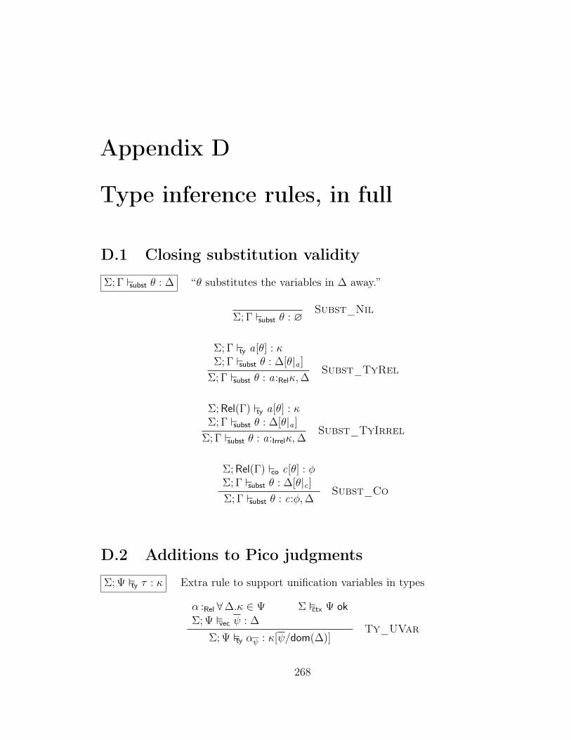
Appendix D

Type inference rules, in full

D.1 Closing substitution validity

Σ; Γ subst θ : ∆ “θ substitutes the variables in ∆ away.”

Σ; Γ subst θ : ∅Subst_Nil

Σ; Γ ty a[θ] : κΣ; Γ subst θ : ∆[θ|a ]

Σ; Γ subst θ : a:Relκ,∆Subst_TyRel

Σ; Rel(Γ) ty a[θ] : κΣ; Γ subst θ : ∆[θ|a ]

Σ; Γ subst θ : a:Irrelκ,∆Subst_TyIrrel

Σ; Rel(Γ) co c[θ] : φΣ; Γ subst θ : ∆[θ|c]Σ; Γ subst θ : c:φ,∆

Subst_Co

D.2 Additions to Pico judgments

Σ; Ψ ty τ : κ Extra rule to support unification variables in types

α :Rel ∀∆.κ ∈ Ψ Σ ctx Ψ okΣ; Ψ vec ψ : ∆

Σ; Ψ ty αψ : κ[ψ/dom(∆)]Ty_UVar

268

Σ; Ψ co γ : φ Extra rule to support unification variables in coercions

ι : ∀∆.φ ∈ Ψ Σ ctx Ψ okΣ; Ψ vec ψ : ∆

Σ; Ψ co ιψ : φ[ψ/dom(∆)]Co_UVar

Σ ctx Ψ ok Extra rules to support binding unification variables

Σ; Rel(Ψ,∆) ty κ : Type Σ ctx Ψ ok

Σ ctx Ψ, α :ρ ∀∆.κ okCtx_UTyVar

Σ; Rel(Ψ,∆) prop φ ok Σ ctx Ψ ok

Σ ctx Ψ, ι : ∀∆.φ okCtx_UCoVar

D.3 Zonker validity

Σ; Ψ z Θ : Ω “Θ zonks all the unification variables in Ω.”

Σ; Ψ z ∅ : ∅Zonk_Nil

Σ; Ψ,∆ ty τ : κΣ; Ψ z Θ : Ω[∀ dom(∆).τ/α]

Σ; Ψ z ∀ dom(∆).τ/α,Θ : α :Rel ∀∆.κ,ΩZonk_TyVarRel

Σ; Rel(Ψ,∆) ty τ : κΣ; Ψ z Θ : Ω[∀ dom(∆).τ/α]

Σ; Ψ z ∀ dom(∆).τ/α,Θ : α :Irrel ∀∆.κ,ΩZonk_TyVarIrrel

Σ; Ψ,∆ co γ : φΣ; Ψ z Θ : Ω[∀ dom(∆).γ/ι]

Σ; Ψ z ∀ dom(∆).γ/ι,Θ : ι : ∀∆.φ,ΩZonk_CoVar

D.4 Synthesis

Σ; Ψ ty t τ : κ a Ω Synthesize a type with no invisible binders.

269

Σ; Ψ ∗ty t τ : κ a Ω1

Specinst κ ψ;κ′ a Ω2

Σ; Ψ ty t τ ψ : κ′ a Ω1,Ω2

ITy_Inst

Σ; Ψ ∗ty t τ : κ a Ω Synthesize a type, perhaps with specified binders.

a:Relκ ∈ Ψ Infinst κ ψ;κ′ a Ω

Σ; Ψ ∗ty a a ψ : κ′ a Ω

ITy_Var

Σ; Ψ ty t1 τ1 : κ0 a Ω1

fun κ0; Rel γ; Π; a; ρ;κ1;κ2 a Ω2

Σ; Ψ,Ω1,Ω2; ρ ∗arg t2 : κ1 ψ2; τ2 a Ω3

Σ; Ψ ∗ty t1 t2 (τ1 B γ)ψ2 : κ2[τ2/a] a Ω1,Ω2,Ω3

ITy_App

Σ; Ψ ∗ty t1 τ1 : ΠSpeca:ρκ1. κ2 a Ω1

Σ; Ψ,Ω1; ρ ∗arg t2 : κ1 ψ2; τ2 a Ω2

Σ; Ψ ∗ty t1 @t2 τ1 ψ2 : κ2[τ2/a] a Ω1,Ω2

ITy_AppSpec

Σ; Rel(Ψ) pt s σ a Ω1

Σ; Ψ,Ω1 ∗ty t : σ τ a Ω2

Σ; Ψ ∗ty (t :: s) τ : σ a Ω1,Ω2

ITy_Annot

Σ; Ψ ty t0 τ0 : κ0 a Ω0

Σ; Ψ,Ω0 scrut alt;κ0 γ; ∆;H ′; τ a Ω′0freshα Ω′ = Ω0,Ω

′0, α:IrrelType

∀i , Σ; Ψ,Ω′; ’Π∆.H ′ τ ; τ0 B γ alt alti : α alti a Ωi

alt′

= make_exhaustive(alt ;κ)

Σ; Ψ ∗ty case t0 of alt caseα (τ0 B γ) of alt

′: α a Ω′,Ω

ITy_Case

Σ; Ψ q qvar a : κ1; ν a Ω1

Σ; Ψ,Ω1, a:Relκ1 ∗ty t τ : κ2 a Ω2

Ω2 → a:Relκ1 Ω′2; ξ

Σ; Ψ ∗ty λqvar. t λa:Relκ1. (τ [ξ]) :

˜Πνa:Relκ1. (κ2[ξ]) a Ω1,Ω′2

ITy_Lam

Σ; Ψ q qvar a : κ1; ν a Ω1

Σ; Ψ,Ω1, a:Irrelκ1 ∗ty t τ : κ2 a Ω2

Ω2 → a:Irrelκ1 Ω′2; ξ

Σ; Ψ ∗ty Λqvar. t λa:Irrelκ1. (τ [ξ]) :

˜Πνa:Relκ1. (κ2[ξ]) a Ω1,Ω′2

ITy_LamIrrel

270

Σ; Ψ ty t1 : Type τ1 a Ω1

Σ; Ψ ty t2 : Type τ2 a Ω2

a # τ2

Σ; Ψ ∗ty t1 → t2

˜ΠReqa:Relτ1. τ2 : Type a Ω1,Ω2

ITy_Arrow

Σ; Ψ ty t1 : Type τ1 a Ω1

Σ; Ψ ty t2 : Type τ2 a Ω2

a # τ2

Σ; Ψ ∗ty t1

′→ t2 ’ΠReqa:Relτ1. τ2 : Type a Ω1,Ω2

ITy_MArrow

Σ; Ψ ty t τ : κ a Ω1

fun κ; Rel γ;˜Π; a; Rel;κ1;κ2 a Ω2

Σ; Rel(Ψ,Ω1,Ω2) ty κ2 : Typefresh ι Ω = Ω1,Ω2, ι:κ2 ∼ κ1

Σ; Ψ ∗ty fix t fix (τ B (γ #

˜Πa:Rel〈κ1〉. ι)) : κ1 a Ω

ITy_Fix

Σ; Ψ ∗ty t1 τ1 : κ1 a Ω

Σ; Ψ,Ω, x :Relκ1 ∗ty t2 τ2 : κ2 a Ω2

Ω2 → x :Relκ1 Ω′2; ξ

Σ; Ψ ∗ty let x := t1 in t2 (λx :Relκ1. (τ2[ξ])) τ1 : κ2[ξ][τ1/x ] a Ω,Ω′2

ITy_Let

D.5 Checking

Σ; Ψ ty t : κ τ a Ω Check against a type with no invisible binders.

Σ; Ψ ty t0 τ0 : κ0 a Ω0

Σ; Ψ,Ω0 scrut alt;κ0 γ; ∆;H ′; τ a Ω′0Ω′ = Ω0,Ω

′0

∀i , Σ; Ψ,Ω′; ’Π∆.H ′ τ ; τ0 B γ altc alti : κ alti a Ωi

alt′

= make_exhaustive(alt ;κ)

Σ; Ψ ty case t0 of alt : κ caseκ (τ0 B γ) of alt′ a Ω′,Ω

ITyC_Case

271

fun κ; Rel γ;˜Π; a; Rel;κ1;κ2 a Ω0

¬(a # κ2)Σ; Rel(Ψ) pt s κ′1 a Ω1

Ω = Ω0,Ω1, ι:κ1 ∼ κ′1Σ; Ψ,Ω, b:Relκ

′1∗ty t : κ2[b B sym ι/a] τ a Ω2

Ω2 → b:Relκ′1 Ω′2; ξ

η = κ2[(a B ι)B sym ι/a] ≈〈Type〉 κ2

τ0 = (λa:Relκ1. (τ [ξ][a B ι/b]B η))B sym γ

Σ; Ψ ty λ(a :: s). t : κ τ0 a Ω,Ω′2ITyC_LamDep

fun κ; Rel γ;˜Π; a; Rel;κ1;κ2 a Ω0

Σ; Ψ aq aqvar : κ1 b : κ′1; x .τ1 a Ω1

Σ; Ψ,Ω0,Ω1, b:Relκ′1∗ty t : κ2 τ a Ω2

Ω2 → b:Relκ′1 Ω′2; ξ

Ω′ = Ω0,Ω1,Ω′2

Σ; Ψ ty λaqvar. t : κ (λa:Relκ1. τ [ξ][τ1[a/x ]/b])B sym γ a Ω′ITyC_Lam

fun κ; Irrel γ;˜Π; a; Irrel;κ1;κ2 a Ω0

¬(a # κ2)Σ; Rel(Ψ) pt s κ′1 a Ω1

Ω = Ω0,Ω1, ι:κ1 ∼ κ′1Σ; Ψ,Ω, b:Irrelκ

′1∗ty t : κ2[b B sym ι/a] τ a Ω2

Ω2 → b:Irrelκ′1 Ω′2; ξ

η = κ2[(a B ι)B sym ι/a] ≈〈Type〉 κ2

τ0 = (λa:Irrelκ1. (τ [ξ][a B ι/b]B η))B sym γ

Σ; Ψ ty Λ(a :: s). t : κ τ0 a Ω,Ω′2ITyC_LamIrrelDep

fun κ; Irrel γ;˜Π; a; Irrel;κ1;κ2 a Ω0

Σ; Ψ aq aqvar : κ1 b : κ′1; x .τ1 a Ω1

Σ; Ψ,Ω0,Ω1, b:Irrelκ′1∗ty t : κ2 τ a Ω2

Ω2 → b:Irrelκ′1 Ω′2; ξ

τ0 = (λa:Irrelκ1. τ [ξ][τ1[a/x ]/b])B sym γ

Σ; Ψ ty Λaqvar. t : κ τ0 a Ω0,Ω1,Ω′2ITyC_LamIrrel

Σ; Ψ ty t :˜ΠReqa:Relκ. κ τ a Ω

Σ; Ψ ty fix t : κ fix τ a ΩITyC_Fix

272

Σ; Ψ ∗ty t τ : κ1 a Ω

pre κ2 ∆;κ′2; τ2

Ω → ∆ Ω′; ξ1

κ1[ξ1] ≤∗ κ′2 τ ′2 a Ω2

Ω2 → ∆ Ω′2; ξ2

Σ; Ψ ty t : κ2 τ2 (λ∆. τ ′2[ξ2] τ [ξ1]) a Ω′,Ω′2ITyC_Infer

Σ; Ψ ∗ty t : κ τ a Ω Check against a type that may have specified binders.

¬(a # κ2)Σ; Rel(Ψ) pt s κ′1 a Ω1

Ω = Ω1, ι:κ1 ∼ κ′1Σ; Ψ,Ω, b:Relκ

′1∗ty t : κ2[b B sym ι/a] τ a Ω2

Ω2 → b:Relκ′1 Ω′2; ξ

η = κ2[(a B ι)B sym ι/a] ≈〈Type〉 κ2

τ0 = λa:Relκ1. (τ [ξ][a B ι/b]B η)

Σ; Ψ ∗ty λ@(a :: s). t :

˜ΠSpeca:Relκ1. κ2 τ0 a Ω,Ω′2

ITyC_LamInvisDep

Σ; Ψ aq aqvar : κ1 b : κ′1; x .τ1 a Ω1

Σ; Ψ,Ω1, b:Relκ′1∗ty t : κ2 τ a Ω2

Ω2 → b:Relκ′1 Ω′2; ξ

τ0 = λa:Relκ1. τ [ξ][τ1[a/x ]/b]

Σ; Ψ ∗ty λ@aqvar. t :

˜ΠSpeca:Relκ1. κ2 τ0 a Ω1,Ω′2

ITyC_LamInvis

¬(a # κ2)Σ; Rel(Ψ) pt s κ′1 a Ω1

Ω = Ω1, ι:κ1 ∼ κ′1Σ; Ψ,Ω, b:Irrelκ

′1∗ty t : κ2[b B sym ι/a] τ a Ω2

Ω2 → b:Irrelκ′1 Ω′2; ξ

η = κ2[(a B ι)B sym ι/a] ≈〈Type〉 κ2

τ0 = λa:Irrelκ1. (τ [ξ][a B ι/b]B η)

Σ; Ψ ∗ty Λ@(a :: s). t :

˜ΠSpeca:Irrelκ1. κ2 τ0 a Ω,Ω′2

ITyC_LamInvisIrrelDep

Σ; Ψ aq aqvar : κ1 b : κ′1; x .τ1 a Ω1

Σ; Ψ,Ω1, b:Irrelκ′1∗ty t : κ2 τ a Ω2

Ω2 → b:Irrelκ′1 Ω′2; ξ

τ0 = λa:Irrelκ1. τ [ξ][τ1[a/x ]/b]

Σ; Ψ ∗ty Λ@aqvar. t :

˜ΠSpeca:Irrelκ1. κ2 τ0 a Ω1,Ω′2

ITyC_LamInvisIrrel

273

Σ; Ψ ∗ty t1 τ1 : κ1 a Ω

Σ; Ψ,Ω, x :Relκ1 ∗ty t2 : κ τ2 a Ω2

Ω2 → x :Relκ1 Ω′2; ξ

Σ; Ψ ∗ty let x := t1 in t2 : κ (λx :Relκ1. (τ2[ξ])) τ1 a Ω,Ω′2

ITyC_Let

ν ≤ SpecΣ; Ψ, $a:ρκ1 ∗ty t : κ2 τ a ΩΩ → $a:ρκ1 Ω′; ξ

Σ; Ψ ∗ty t :

˜Πν$a:ρκ1. κ2 λ$a:ρκ1. τ [ξ] a Ω′

ITyC_Skol

Σ; Ψ ty t : κ τ a Ω

Σ; Ψ ∗ty t : κ τ a Ω

ITyC_Otherwise

Σ; Ψ pt s τ a Ω Check a poly-type (which always has type Type).

pi quant Π; ρΣ; Ψ q qvar a : κ; ν a ΩΣ; Ψ,Ω, a:ρκ pt s σ a Ω2

Ω2 → a:ρκ Ω′2; ξ

Σ; Ψ pt ∀ qvar. s Πνa:ρκ. (σ[ξ]) a Ω,Ω′2IPtC_Pi

Σ; Ψ ty t : Type τ a Ω1

Σ; Ψ,Ω1, $a:Relτ pt s σ a Ω2

Ω2 → $a:Relτ Ω′2; ξ

Σ; Ψ pt t⇒ s ˜ΠInf$a:Relτ. (σ[ξ]) a Ω1,Ω′2

IPtC_Constrained

Σ; Ψ ty t : Type τ a Ω

Σ; Ψ pt t τ a ΩIPtC_Mono

D.6 Inference for auxiliary syntactic elements

Σ; Ψ; ρ ∗arg t : κ ψ; τ a Ω Check a function argument against its known type.

Σ; Ψ ∗ty t : κ τ a Ω

Σ; Ψ; Rel ∗arg t : κ τ ; τ a ΩIArg_Rel

Σ; Rel(Ψ) ∗ty t : κ τ a Ω

Σ; Ψ; Irrel ∗arg t : κ τ; τ a ΩIArg_Irrel

274

Σ; Ψ;κ0; τ0 alt alt : κ alt a Ω Synth. a case alt. against a unification variable.

Σ tc H : ∆1; ∆2;H ′ ∆3,∆4 = ∆2[τ/dom(∆1)]dom(∆3) = x dom(∆4) = dom(∆′)matchdom(∆3)(types(∆4); types(∆′)) = Just θΣ; Ψ,∆3 ty t : κ τ a ΩΩ → ∆3 Ω′; ξ∆′3 = ∆3, c:τ0 ∼ Hτ x

Σ; Ψ; ’Π∆′.H ′ τ ; τ0 alt H x → t : κ H → λ∆′3. (τ [ξ]) a Ω′IAlt_Con

Σ; Ψ ty t : κ τ a Ω

Σ; Ψ;κ0; τ0 alt _→ t : κ _→ τ a ΩIAlt_Default

Σ; Ψ;κ0; τ0 altc alt : κ alt a Ω Check a case alt. against a known result type.

Σ tc H : ∆1; ∆2;H ′ ∆3,∆4 = ∆2[τ/dom(∆1)]dom(∆3) = x dom(∆4) = dom(∆′)matchdom(∆3)(types(∆4); types(∆′)) = Just θ0

∆′3 = ∆3, c:τ0 ∼ Hτ xΣ; Ψ,∆′3 ty t : κ τ a ΩΩ → ∆′3 Ω′; ξ

Σ; Ψ; ’Π∆′.H ′ τ ; τ0 altc H x → t : κ H → λ∆′3. (τ [ξ]) a Ω′IAltC_Con

Σ; Ψ ty t : κ τ a Ω

Σ; Ψ;κ0; τ0 altc _→ t : κ _→ τ a ΩIAltC_Default

Σ; Ψ q qvar a : κ; ν a Ω Synthesize a bound variable.

Σ; Ψ aq aqvar a : κ a Ω

Σ; Ψ q aqvar a : κ; Req a ΩIQVar_Req

Σ; Ψ aq aqvar a : κ a Ω

Σ; Ψ q @aqvar a : κ; Spec a ΩIQVar_Spec

Σ; Ψ aq aqvar a : κ a Ω Synthesize a bound variable (w/o vis. marker).

fresh β

Σ; Ψ aq a a : β a β:IrrelTypeIAQVar_Var

Σ; Rel(Ψ) pt s σ a Ω

Σ; Ψ aq (a :: s) a : σ a ΩIAQVar_Annot

275

Σ; Ψ aq aqvar : κ a : κ′; x .τ a Ω Check a bound variable (w/o vis. marker).

Σ; Ψ aq a : κ a : κ; x .x a ∅IAQVarC_Var

Σ; Rel(Ψ) pt s σ a Ω1

κ ≤ σ τ a Ω2

Σ; Ψ aq (a :: s) : κ a : σ; x .τ x a Ω1,Ω2

IAQVarC_Annot

pi quant Π; ρ Interpret a quantifier.

pi ∀ ˜Π; Irrel

IQu_ForAll

pi ′∀ ’Π; IrrelIQu_MForAll

pi Π ˜Π; Rel

IQu_Pi

pi ′Π ’Π; RelIQu_MPi

D.7 Kind conversionsfun κ; ρ1 γ; Π; a; ρ2;κ1;κ2 a Ω Extract out the parts of a function kind.

fun ΠReqa:ρκ1. κ2; ρ0 〈ΠReqa:ρκ1. κ2〉; Π; a; ρ;κ1;κ2 a ∅IFun_Id

fresh ι fresh β1, β2

Ω = β1:IrrelType, β2:IrrelType, ι:κ0 ∼˜ΠReqa:ρβ1. β2

fun κ0; ρ ι;˜Π; a; ρ; β1; β2 a Ω

IFun_Cast

Σ; Ψ scrut alt;κ γ; ∆;H ; τ a Ω Extract out the parts of a scrutinee’s kind.

Σ; Rel(Ψ) ty H τ : Type

Σ; Ψ scrut alt; ’Π∆.H τ 〈’Π∆.H τ〉; ∆;H ; τ a ∅IScrut_Id

276

Σ tc H : a:Irrelκ; ∆2;H ′

freshα fresh ιΩ = α:Irrelκ[α/a], ι:κ ∼ H ′ α

Σ; Ψ scrut (H x → t; alt);κ ι;∅;H ′;α a ΩIScrut_Cast

D.8 Instantiationνinst κ ψ;κ′ a Ω Instantiate so that a type’s first binder is more visible than ν.

freshα ν2 ≤ ν1

ν1inst κ2[α/a] ψ;κ′2 a Ω

ν1inst Πν2a:Relκ1. κ2 α, ψ;κ′2 a α:Relκ1,Ω

IInst_Rel

freshα ν2 ≤ ν1

ν1inst κ2[α/a] ψ;κ′2 a Ω

ν1inst Πν2a:Relκ1. κ2 α, ψ;κ′2 a α:Irrelκ1,Ω

IInst_Irrel

fresh ιν1inst κ2[ι/c] ψ;κ′2 a Ω

ν1inst ΠInfc:φ. κ ι, ψ;κ′2 a ι:φ,Ω

IInst_Co

ν1inst κ ∅;κ a ∅

IInst_Done

ν1 ≤ ν2 “Less-visible-than“ relation

ν ≤ νIVis_Refl

ν1 ≤ ν2 ν2 ≤ ν3

ν1 ≤ ν3

IVis_Trans

Inf ≤ SpecIVis_InfSpec

Spec ≤ ReqIVis_SpecReq

277

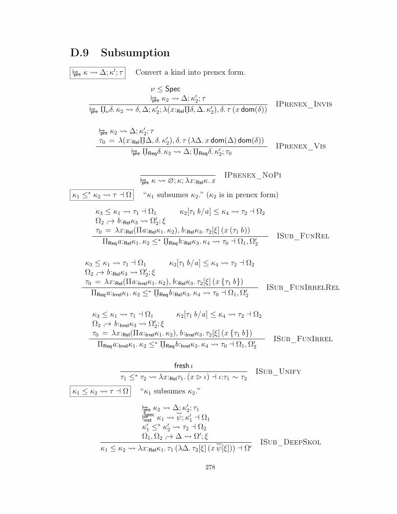
D.9 Subsumption

pre κ ∆;κ′; τ Convert a kind into prenex form.

ν ≤ Specpre κ2 ∆;κ′2; τ

pre˜Πνδ. κ2 δ,∆;κ′2;λ(x :Rel

˜Πδ,∆. κ′2), δ. τ (x dom(δ))

IPrenex_Invis

pre κ2 ∆;κ′2; ττ0 = λ(x :Rel

˜Π∆, δ. κ′2), δ. τ (λ∆. x dom(∆) dom(δ))

pre˜ΠReqδ. κ2 ∆;

˜ΠReqδ. κ′2; τ0

IPrenex_Vis

pre κ ∅;κ;λx :Relκ. xIPrenex_NoPi

κ1 ≤∗ κ2 τ a Ω “κ1 subsumes κ2.” (κ2 is in prenex form)

κ3 ≤ κ1 τ1 a Ω1 κ2[τ1 b/a] ≤ κ4 τ2 a Ω2

Ω2 → b:Relκ3 Ω′2; ξτ0 = λx :Rel(Πa:Relκ1. κ2), b:Relκ3. τ2[ξ] (x (τ1 b))

ΠReqa:Relκ1. κ2 ≤∗˜ΠReqb:Relκ3. κ4 τ0 a Ω1,Ω′2

ISub_FunRel

κ3 ≤ κ1 τ1 a Ω1 κ2[τ1 b/a] ≤ κ4 τ2 a Ω2

Ω2 → b:Relκ3 Ω′2; ξτ0 = λx :Rel(Πa:Irrelκ1. κ2), b:Relκ3. τ2[ξ] (x τ1 b)

ΠReqa:Irrelκ1. κ2 ≤∗˜ΠReqb:Relκ3. κ4 τ0 a Ω1,Ω′2

ISub_FunIrrelRel

κ3 ≤ κ1 τ1 a Ω1 κ2[τ1 b/a] ≤ κ4 τ2 a Ω2

Ω2 → b:Irrelκ3 Ω′2; ξτ0 = λx :Rel(Πa:Irrelκ1. κ2), b:Irrelκ3. τ2[ξ] (x τ1 b)

ΠReqa:Irrelκ1. κ2 ≤∗˜ΠReqb:Irrelκ3. κ4 τ0 a Ω1,Ω′2

ISub_FunIrrel

fresh ι

τ1 ≤∗ τ2 λx :Relτ1. (x B ι) a ι:τ1 ∼ τ2

ISub_Unify

κ1 ≤ κ2 τ a Ω “κ1 subsumes κ2.”

pre κ2 ∆;κ′2; τ1

Specinst κ1 ψ;κ′1 a Ω1

κ′1 ≤∗ κ′2 τ2 a Ω2

Ω1,Ω2 → ∆ Ω′; ξ

κ1 ≤ κ2 λx :Relκ1. τ1 (λ∆. τ2[ξ] (x ψ[ξ])) a Ω′ISub_DeepSkol

278

D.10 GeneralizationΩ → ∆ Ω′; ξ Generalize Ω over ∆.

∅ → ∆ ∅;∅IGen_Nil

ξ0 = α 7→ dom(∆) Ω[ξ0] → ∆ Ω′; ξ

α :ρ ∀∆′.κ,Ω → ∆ α :ρ ∀∆,∆′.κ,Ω′; ξ0, ξIGen_TyVar

ξ0 = ι 7→ dom(∆) Ω[ξ0] → ∆ Ω′; ξ

ι : ∀∆′.φ,Ω → ∆ ι : ∀∆,∆′.φ,Ω′; ξ0, ξIGen_CoVar

D.11 Programs

Σ; Γ decl decl x : κ := τ Check a Haskell declaration.

Σ; Γ ty t τ : κ a ΩΣ; Γ solv Ω ∆; Θτ ′ = λ∆. (τ [Θ]) κ′ =

˜ΠInf∆. (κ[Θ])

Σ; Γ decl x := t x : κ′ := τ ′IDecl_Synthesize

Σ; Γ pt s σ a Ω1

Σ; Rel(Γ) solv Rel(Ω1) ∆1; Θ1

σ′ =˜ΠInf∆1. (σ[Θ1])

Σ; Γ ∗ty t : σ′ τ a Ω2

Σ; Γ solv Ω2 ∅; Θ2

τ ′ = τ [Θ2]

Σ; Γ decl x :: s := t x : σ′ := τ ′IDecl_Check

Σ; Γ prog prog Γ′; θ Check a Haskell program.

Σ; Γ prog ∅ ∅;∅IProg_Nil

279

Σ; Γ decl decl x : κ := τΣ; Γ, x :Relκ, c:x ∼ τ prog prog Γ′; θ

Σ; Γ prog decl; prog x :Relκ, c:x ∼ τ,Γ′; (τ/x , 〈τ〉/c) θIProg_Decl

280

Appendix E

Proofs about the Bake algorithm

Throughout this appendix, I use a convention whereby in any case where the rule underconsideration is printed, any metavariable names in the rule shadow any metavariablenames in the lemma or theorem statement.

E.1 Type inference judgment propertiesDefinition E.1 (Judgments with unification variables). I write judgments with a newturnstile ; these judgments are identical to the corresponding judgments written witha ` except with the new rules as given in Appendix D. All lemmas proved over the oldjudgments hold over the new ones, noting that the new UVar rules are unaffected bycontext extension.

Definition E.2 (Generalized judgments). I sometimes write Σ; Ψ J , where Jstands for a judgment, one of the judgments headed by ty, co, prop, alt, vec, ctx, or s.Similarly, I write J [θ] to denote substitution in the component parts of the judgmentJ .

Lemma E.3 (Extension).

1. If Σ; Γ ` J , then Σ; Γ J .2. If Σ; Γ J and J mentions no unification variables, then Σ; Γ ` J .

Proof. The difference between the ` judgments and the judgments is only theaddition of new rules for new forms. No previously valid derivations are affected.Note that, although we can’t prove it now, the “mentions no unification variables” isredundant, as shown by Lemma E.11, below.

E.2 Properties adopted from Appendix CRemark. By the straightforward extension of the Rel(·) operation, all previous lemmas(Lemma C.3, Lemma C.4, Lemma C.5, Lemma C.6) dealing with contexts and relevance

281

remain true under the judgments.

Lemma E.4 (Type variable kinds [Lemma C.7]). (as stated previously, but withreference to judgments)

Proof. As before; the new forms do not pose any problems.

Lemma E.5 (Unification type variable kinds). If Σ ctx Ψ ok and α :ρ ∀∆.κ ∈ Ψ, thenthere exists Ψ′ such that Ψ′ ⊆ Rel(Ψ) and Σ; Ψ′,Rel(∆) ty κ : Type. Furthermore, thesize of the derivation of Σ; Ψ′,Rel(∆) ty κ : Type is smaller than that of Σ ctx Ψ ok.

Proof. Straightforward induction on Σ ctx Ψ ok.

Lemma E.6 (Coercion variable kinds [Lemma C.8]). (as stated previously, but withreference to judgments)

Proof. As before; the new forms do not pose any problems.

Lemma E.7 (Unification coercion variable kinds). If Σ ctx Ψ ok and ι : ∀∆.φ ∈ Ψ,then there exists Ψ′ such that Ψ′ ⊆ Rel(Ψ) and Σ; Ψ′,Rel(∆) prop φ ok. Furthermore,the size of the derivation of Σ; Ψ′,Rel(∆) prop φ ok is smaller than that of Σ ctx Ψ ok.

Proof. Straightforward induction on Σ ctx Ψ ok.

Lemma E.8 (Context regularity [Lemma C.9]). (as stated previously, but with refer-ence to judgments)

Proof. As before; the new forms do not pose any problems.

Lemma E.9 (Weakening [Lemma C.10]). Assume Σ ctx Ψ′ ok and Ψ ⊆ Ψ′. IfΣ; Ψ J , then Σ; Ψ′ J .

Proof. As before; the new forms do not pose any problems.

Lemma E.10 (Strengthening [Lemma C.11]). (as stated previously, but with referenceto judgments)

Proof. As before; the new forms do not pose any problems.

Lemma E.11 (Scoping [Lemma C.12]). (as stated previously, but with reference to judgments)

Proof. We must consider now Ty_UVar and Co_UVar. These cases are similar;let’s focus on Ty_UVar:

α :Rel ∀∆.κ ∈ Ψ Σ ctx Ψ okΣ; Ψ vec ψ : ∆

Σ; Ψ ty αψ : κ[ψ/dom(∆)]Ty_UVar

282

We see that α ∈ dom(Ψ), and the induction hypothesis tells us that the scopingrequirement holds for ψ. Lemma E.5 tells us that Σ; Ψ′,Rel(∆) ty κ : Type for someΨ′ ⊆ Rel(Ψ). This derivation is smaller than the one ending in Ty_UVar, and sowe can use the induction hypothesis to see that fv(κ) ⊆ (dom(Ψ) ∪ dom(∆)).The substitution in the conclusion removes all use of variables in dom(∆), and sofv(κ) ⊆ dom(Ψ) as desired.

Lemma E.12 (Determinacy [Lemma C.20]). (as stated previously, but with referenceto judgments)

Proof. As before.

Lemma E.13 (Type substitution [Lemma C.35]). If Σ; Ψ ty σ : κ and Σ; Ψ, a:ρκ,Ψ′

J , then Σ; Ψ,Ψ′[σ/a] J [σ/a].

Proof. By induction on Σ; Ψ, a:ρκ,Ψ′ J . We consider only the new cases.

Case Ty_UVar:

α :Rel ∀∆.κ ∈ Ψ Σ ctx Ψ okΣ; Ψ vec ψ : ∆

Σ; Ψ ty αψ : κ[ψ/dom(∆)]Ty_UVar

We must prove Σ; Ψ,Ψ′[σ/a] ty αψ[σ/a] : κ[ψ/dom(∆)][σ/a]. (Recall that nor-mal substitutions θ do not map unification variables.) We know α :Rel ∀∆.κ ∈Ψ, a:ρκ,Ψ

′, Σ ctx Ψ, a:ρκ,Ψ′ ok and Σ; Ψ, a:ρκ,Ψ

′ vec ψ : ∆. By the inductionhypothesis, we can conclude Σ ctx Ψ,Ψ′[σ/a] ok and Σ; Ψ,Ψ′[σ/a] vec ψ[σ/a] :∆[σ/a]. We now have two cases, depending on the location of α:

Case α :Rel ∀∆.κ ∈ Ψ: In this case, Lemma E.11 tells us that ∆ cannot mentiona, and thus ∆[σ/a] = ∆. We can thus use α :Rel ∀∆.κ ∈ Ψ to com-plete the premises for Ty_UVar, showing that Σ; Ψ,Ψ′[σ/a] ty αψ[σ/a] :

κ[ψ[σ/a]/dom(∆)]. The kind can be rewritten as κ[σ/a][ψ[σ/a]/dom(∆)]as we know a 6∈ fv(κ). It can then further be rewritten to κ[ψ/dom(∆)][σ/a]as desired.

Case α :Rel ∀∆.κ ∈ Ψ′: It must be the case that α :Rel ∀ (∆[σ/a]).(κ[σ/a]) ∈Ψ′[σ/a]. Rule Ty_UVar then gives us Σ; Ψ,Ψ′[σ/a] ty αψ[σ/a] :

κ[σ/a][ψ[σ/a]/dom(∆)] which can be (see above) rewritten asΣ; Ψ,Ψ′[σ/a] ty αψ[σ/a] : κ[ψ/dom(∆)][σ/a] as desired.

Case Co_UVar: Similar to previous case.

Lemma E.14 (Coercion substitution [Lemma C.36]). If Σ; Ψ co γ : φ andΣ; Ψ, c:φ,Ψ′ J , then Σ; Ψ,Ψ′[γ/c] J [γ/c].

283

Proof. Similar to previous proof.

Lemma E.15 (Vector substitution [Lemma C.37]). If Σ; Ψ vec ψ : ∆ and Σ; Ψ,∆,Ψ′ J , then Σ; Ψ,Ψ′[ψ/dom(∆)] J [ψ/dom(∆)].

Proof. As before, referring to Lemma E.13 and Lemma E.14. Note that this version isgeneralized to work over any judgment J while the previous proof lemma works onlyover ty. This generalization poses no trouble.

E.3 RegularityLemma E.16 (Increasing relevance in vectors). If Σ; Ψ vec ψ : ∆, then Σ; Rel(Ψ) vecψ : Rel(∆).

Proof. Straightforward induction on the typing derivation, appealing to Lemma C.6.

Lemma E.17 (Kind regularity [Lemma C.43]). If Σ; Ψ ty τ : κ, then Σ; Rel(Ψ) ty κ :Type.

Proof. By induction on the typing derivation. We consider only the new case:

Case Ty_UVar:

α :Rel ∀∆.κ ∈ Ψ Σ ctx Ψ okΣ; Ψ vec ψ : ∆

Σ; Ψ ty αψ : κ[ψ/dom(∆)]Ty_UVar

We must prove Σ; Rel(Ψ) ty κ[ψ/dom(∆)] : Type. By Lemma E.8 and LemmaE.5, there exists Ψ′ such that Ψ′ ⊆ Rel(Ψ) and Σ; Ψ′,Rel(∆) ty κ : Type.Lemma E.9 then gives us Σ; Rel(Ψ,∆) ty κ : Type. Lemma E.16 tells us thatΣ; Rel(Ψ) vec ψ : Rel(∆). We can thus use Lemma E.15 to get Σ; Rel(Ψ) tyκ[ψ/dom(∆)] : Type as desired.

Lemma E.18 (Proposition regularity [Lemma C.44]). If Σ; Ψ co γ : φ, thenΣ; Rel(Ψ) prop φ ok.

Proof. The proof for the Co_UVar case is similar to the proof above for Ty_UVar.Other cases are as before.

284

E.4 ZonkingDefinition E.19 (Zonker). A zonker Θ is a substitution from unification variables αand ι to types and coercions, respectively. Each mapping also includes a list of typeand coercion variables under which it is quantified.

Θ ::=∅ |Θ,∀ z .τ/α |Θ,∀ z .γ/ι

Lemma E.20 (Zonker domains). If Σ; Ψ z Θ : Ω, then dom(Θ) = dom(Ω).

Proof. By straightforward induction.

Lemma E.21 (Zonking a relevant type variable). If α :Rel ∀∆.κ ∈ Ω, Σ; Ψ z Θ : Ω,no binding in Ω refers to a later one, and the range of Θ is disjoint from its domain,then there exists τ such that ∀ dom(∆).τ/α ∈ Θ and Σ; Ψ,∆[Θ] ty τ : κ[Θ].

Proof. By induction on Σ; Ψ z Θ : Ω.

Case Zonk_Nil: Impossible, as Ω is empty.

Case Zonk_TyVarRel: We have two cases here:

Case Ω = α :Rel ∀∆.κ,Ω′: We see that Θ = ∀ dom(∆).τ/α,Θ′, satisfying thefirst conclusion. The premise of Zonk_TyVarRel tells us Σ; Ψ,∆ tyτ : κ. By assumption, we know that ∆ and κ cannot refer to α nor anyvariables in Ω′. Thus ∆ = ∆[Θ] and κ = κ[Θ], and thus we can concludeΣ; Ψ,∆[Θ] ty τ : κ[Θ] as desired.

Case Ω = α′ :ρ ∀∆′.κ′,Ω′, with α 6= α′: We see that Θ = ∀ dom(∆′).τ ′/α′,Θ′.Let Θ0 = ∀ dom(∆′).τ ′/α′. We can further see thatα :Rel ∀ (∆[Θ0]).(κ[Θ0]) ∈ Ω′[Θ0] and Σ; Ψ z Θ′ : Ω′[Θ0]. Becausethe range of Θ is disjoint from its domain and the fact that Ω iswell-scoped, we know Ω′[Θ0] must be well-scoped. We can thus usethe induction hypothesis to get τ such that ∀ dom(∆).τ/α ∈ Θ′ andΣ; Ψ,∆[Θ0][Θ

′] ty τ : κ[Θ0][Θ′]. Because Θ is idempotent, we can rewrite

this as Σ; Ψ,∆[Θ] ty τ : κ[Θ] as desired.

Case Zonk_TyVarIrrel: Like second half of previous case.

Case Zonk_CoVar: Like previous case.

Lemma E.22 (Zonking a coercion variable). If ι : ∀∆.φ ∈ Ω, Σ; Ψ z Θ : Ω, nobinding in Ω refers to a later one, and the range of Θ is disjoint from its domain, thenthere exists γ such that ∀ dom(∆).γ/ι ∈ Θ and Σ; Ψ,∆[Θ] co γ : φ[Θ].

Proof. Similar to previous proof.

285

Lemma E.23 (Zonking). If Θ is idempotent, Σ; Ψ z Θ : Ω and Σ; Ψ,Ω,∆2 J , thenΣ; Ψ,∆2[Θ] J [Θ].

Proof. By induction on the derivation Σ; Ψ,Ω,∆2 J .

Case Ty_Var:Σ ctx Γ ok a:Relκ ∈ Γ

Σ; Γ ty a : κTy_Var

We know Σ ctx Ψ,Ω,∆2 ok and a:Relκ ∈ Ψ,Ω,∆2. We must prove Σ; Ψ,∆2[Θ] tya[Θ] : κ[Θ]. Zonking a non-unification variable (like a) has no effect, so we mustprove Σ; Ψ,∆2[Θ] ty a : κ[Θ]. We will use Ty_Var, so we must prove thefollowing:

Σ ctx Ψ,∆2[Θ] ok: By the induction hypothesis.a:Relκ[Θ] ∈ Ψ,∆2[Θ]: From a:Relκ ∈ Ψ,Ω,∆2, we know that a must appear

either in Ψ or in ∆2. If a is in Ψ, we are done, using Lemma E.11 to showthat zonking κ has no effect. If a is in ∆2, then a:Relκ[Θ] must be in ∆2[Θ],and so we are done with this case.

Case Co_Var: Similar to previous case.

Case Ty_UVar:

α :Rel ∀∆.κ ∈ Ψ Σ ctx Ψ okΣ; Ψ vec ψ : ∆

Σ; Ψ ty αψ : κ[ψ/dom(∆)]Ty_UVar

We know Σ; Ψ,Ω,∆2 ty αψ : κ[ψ/dom(∆)] and must prove Σ; Ψ,∆2[Θ] ty αψ[Θ] :

κ[ψ/dom(∆)][Θ]. We further know that Σ; Ψ,Ω,∆2 vec ψ : ∆ By the inductionhypothesis, Σ; Ψ,∆2[Θ] vec ψ[Θ] : ∆[Θ] and Σ ctx Ψ,∆2[Θ] ok. There are thenseveral possibilities:

Case α :Rel ∀∆.κ ∈ Ψ: By Lemma E.20, we know that dom(Θ) = dom(Ω). FromΣ ctx Ψ,Ω,∆2 ok and Lemma E.11 we know that nothing in Ψ can mentionany variable bound in Ω. We also know that αψ[Θ] = αψ[Θ] and κ[Θ] = κ.The telescope ∆ is mentioned in Ψ and therefore is unaffected by thezonking substitution Θ. We can thus conclude that α :Rel ∀∆.κ ∈ Ψ,∆2[Θ]and Σ; Ψ,∆2[Θ] vec ψ[Θ] : ∆. We can thus use Ty_UVar to concludeΣ; Ψ,∆2[Θ] ty αψ[Θ] : κ[ψ[Θ]/dom(∆)]. We can rewrite this kind to beκ[ψ/dom(∆)][Θ] as desired because κ[Θ] = κ.

Case α :Rel ∀∆.κ ∈ Ω: We then use Lemma E.21 to get Σ; Ψ,∆[Θ] ty τ :κ[Θ] and ∀ dom(∆).τ/α ∈ Θ. Thus (by Definition E.19) αψ[Θ] =

τ [ψ[Θ]/dom(∆)]. Lemma E.9 gives us Σ; Ψ,∆2[Θ],∆[Θ] ty τ : κ[Θ].

286

The induction hypothesis tells us that Σ; Ψ,∆2[Θ] vec ψ[Θ] : ∆[Θ].Now, we apply Lemma E.15 to get Σ; Ψ,∆2[Θ] ty τ [ψ[Θ]/dom(∆)] :κ[Θ][ψ[Θ]/dom(∆)], which can easily be rewritten to Σ; Ψ,∆2[Θ] tyτ [ψ[Θ]/dom(∆)] : κ[ψ/dom(∆)][Θ] as desired.

Case Co_UVar: Similar to previous case, but using Lemma E.22.

Other cases: Similar to proof for Lemma C.35.

E.5 SolverThe solver (solv) must have the following properties.

Property E.24 (Solver is sound). If Σ ctx Ψ,Ω ok and Σ; Ψ solv Ω ∆; Θ, then Θis idempotent, Σ ctx Ψ,∆ ok, and Σ; Ψ,∆ z Θ : Ω.

E.6 Supporting functionsDefinition E.25 (make_exhaustive). Define make_exhaustive(alt ;κ) as follows:

make_exhaustive(alt ;κ) = alt ((_→ τ) ∈ alt)

make_exhaustive(alt ;κ) = alt ;_→ errorκ "failed match" (otherwise)

E.7 Supporting lemmasLemma E.26 (Vector extension). If Σ; Ψ,∆,Ψ′ vec ψ : ∆′, then Σ; Ψ,∆,Ψ′ vecdom(∆), ψ : ∆,∆′.

Proof. We know Σ ctx Ψ,∆,Ψ′ ok by Lemma E.8. Proceed by induction on thestructure of ∆.

Case ∆ = ∅: Trivial.

Case ∆ = a:ρκ,∆1: To use Vec_TyRel, we must show Σ; Ψ,∆,Ψ′ ty a : κ (whichis by Ty_Var) and Σ; Ψ,∆,Ψ′ vec dom(∆1), ψ : (∆1,∆

′)[a/a]. The substitutionclearly has no effect, so we are done by the induction hypothesis.

Other cases: Similar.

Lemma E.27 (Type variables instantiation). If Σ ctx a:Irrelκ ok, then Σ ctx

b:Irrelκ[b/a] ok.

287

Proof. By induction on the length of κ.

Case κ = ∅: Trivial.

Case κ = κ′, κ0: Here, we know a = a ′, a0 and b = b′, b0. Our assumption is that

Σ ctx a ′:Irrelκ′, a0:Irrelκ0 ok. Inversion (of Ctx_TyVar) gives us Σ; a ′:Relκ

′ty

κ0 : Type and Σ ctx a ′:Irrelκ′ ok. The induction hypothesis tells us Σ ctx

b′:Irrelκ

′[b′/a ′] ok. We must show Σ; b

′:Relκ

′[b′/a ′] ty κ0[b

′/a ′] : Type. Use Lemma

C.10 (Weakening) to get Σ; b′:Relκ

′[b′/a ′], a ′:Relκ

′ty κ0 : Type. Lemma C.39

gives us Σ; b′:Relκ

′[b′/a ′] vec b

′: (b

′:Relκ

′[b′/a ′]). We can thus use Lemma C.37 to

get Σ; b′:Relκ

′[b′/a ′] ty κ0[b

′/a ′] : Type as desired. We then use Ctx_TyVar

and we are done.

Lemma E.28 (Decreasing relevance). If Σ ctx Rel(Ψ) ok, then Σ ctx Ψ ok.

Proof. Straightforward induction on Σ ctx Rel(Ψ) ok.

Lemma E.29 (Closing substitution substitution).

1. If Σ; Γ, a:Relκ,Γ′

subst θ : ∆ and Σ; Γ ty σ : κ, then Σ; Γ,Γ′[σ/a] subst σ/a θ :∆[σ/a].

2. If Σ; Γ, a:Irrelκ,Γ′

subst θ : ∆ and Σ; Rel(Γ) ty σ : κ, then Σ; Γ,Γ′[σ/a] subst

σ/a θ : ∆[σ/a].

3. If Σ; Γ, c:φ,Γ′ subst θ : ∆ and Σ; Γ co γ : φ, then Σ; Γ,Γ′[γ/c] subst γ/c θ :∆[γ/c]

Proof. By induction on the subst derivation. We will consider the type substitutioncase; the others are similar.

Case Subst_Nil: Trivial.

Case Subst_TyRel: In this case, we know Σ; Γ, a:ρκ,Γ′

subst θ : b:Relκ0,∆ andmust show Σ; Γ,Γ′[σ/a] subst σ/a θ : b:Relκ0[σ/a],∆[σ/a]. Inverting gives usΣ; Γ, a:ρκ,Γ

′ty b[θ] : κ0 and Σ; Γ, a:ρκ,Γ

′subst θ : ∆[θ|b ]. To use Subst_TyRel,

we must show Σ; Γ,Γ′[σ/a] ty b[σ/a θ] : κ0[σ/a] and Σ; Γ,Γ′[σ/a] subst σ/a θ :∆[σ/a][(σ/a θ)|b ]. The first of these is directly from the induction hypothesis.The induction hypothesis also gives us Σ; Γ,Γ′[σ/a] subst σ/a θ : ∆[θ|b][σ/a].We are left only to show that ∆[θ|b ][σ/a] = ∆[σ/a][(σ/a θ)|b ]. On the right,we care only about θ’s action on b, so we can rewrite to ∆[σ/a][σ/a (θ|b)],which can then be rewritten to ∆[θ|b ][σ/a] as desired.

Case Subst_TyIrrel: Similar to previous case.

Case Subst_Co: Similar to previous case.

288

Lemma E.30 (Closing substitution). Assume Σ; Γ subst θ : ∆. Let θ′ = θ|dom(∆).

1. If Σ; Γ,∆,Γ′ ty τ : κ, then Σ; Γ,Γ′[θ′] ty τ [θ′] : κ[θ′].

2. If Σ; Γ,∆,Γ′ co γ : φ, then Σ; Γ,Γ′[θ′] co γ[θ′] : φ[θ′].

3. If Σ; Γ,∆,Γ′ prop φ ok, then Σ; Γ,Γ′[θ′] prop φ[θ′] ok.

4. If Σ; Γ,∆,Γ′;σ0 `τ0alt alt : κ, then Σ; Γ,Γ′[θ′];σ0[θ′] `τ0[θ′]alt alt [θ′] : κ[θ′].

5. If Σ; Γ,∆,Γ′ vec ψ : ∆, then Σ; Γ,Γ′[θ′] vec ψ[θ′] : ∆[θ′].

6. If Σ ctx Γ,∆,Γ′ ok, then Σ ctx Γ,Γ′[θ′] ok.

7. If Σ; Γ,∆,Γ′ s τ −→ τ ′, then Σ; Γ,Γ′[θ′] s τ [θ′] −→ τ ′[θ′].

Proof. By induction on Σ; Γ subst θ : ∆. By analogy with the Σ; Ψ J notation, I willuse Σ; Γ ` J to refer collectively to the judgments over which this lemma is defined.

Case Subst_Nil: In this case, ∆ = ∅ and we are done by assumption.

Case Subst_TyRel:

Σ; Γ ty a[θ] : κΣ; Γ subst θ : ∆[θ|a ]

Σ; Γ subst θ : a:Relκ,∆Subst_TyRel

We know Σ; Γ subst θ : a:Relκ,∆ and Σ; Γ, a:Relκ,∆,Γ′ ` J . We must prove

Σ; Γ ` J [θ|a,dom(∆)]. We know Σ; Γ ty a[θ] : κ and thus we can use Lemma C.35to get Σ; Γ,∆[θ|a ],Γ′[θ|a ] ` J [θ|a ]. We then use the induction hypothesis to getΣ; Γ ` J [θ|a ][θ|dom(∆)]. It remains only to show that θ|a θ|dom(∆) = θ|a,dom(∆).This amounts to showing that dom(∆) # a[θ]. We have this by Lemma C.12,and so we are done.

Case Subst_TyIrrel: Similar to previous case.

Case Subst_Co: Similar to previous case, referring to Lemma C.36.

E.8 GeneralizationDefinition E.31 (Generalizer). A generalizer ξ is a mapping from unification variablesto vectors:

ξ ::=∅ | ξ, α 7→ ψ | ξ, ι 7→ ψ

289

A generalizer can be applied postfix as a function. It operates only on occurrences ofunification variables, acting homomorphically on all other forms:

α 7→ ψ1 ∈ ξ ⇒ αψ2[ξ] = αψ1,ψ2

otherwise αψ[ξ] = αψ[ξ]

ι 7→ ψ1 ∈ ξ ⇒ ιψ2[ξ] = ιψ1,ψ2

otherwise ιψ[ξ] = ιψ[ξ]

Lemma E.32 (Generalization by type variable). If Σ; Ψ,∆, α :ρ ∀∆′.κ,Ψ′ J , thenΣ; Ψ, α :ρ ∀∆,∆′.κ,∆,Ψ′[α 7→ dom(∆)] J [α 7→ dom(∆)].

Proof. Let ξ = α 7→ dom(∆). Proceed by induction on the typing derivation. Theonly interesting case is for unification variables:

Case Ty_UVar: Here, we know Σ; Ψ,∆, α :ρ ∀∆′.κ,Ψ′ ty βψ : κ0 and must showΣ; Ψ, α :ρ ∀∆,∆′.κ,∆,Ψ′[ξ] ty βψ[ξ] : κ0[ξ]. We have two cases:

Case α = β: In this case, we know ρ = Rel and κ0 = κ[ψ/dom(∆′)]. In orderto use Ty_UVar, we must show Σ ctx Ψ, α :Rel ∀∆,∆′.κ,∆,Ψ′[ξ] ok (whichwe get from the induction hypothesis) and Σ; Ψ, α :Rel ∀∆,∆′.κ,∆,Ψ′[ξ] vecdom(∆), ψ : ∆,∆′. We know Σ; Ψ,∆, α :ρ ∀∆′.κ,Ψ′ vec ψ : ∆′. The induc-tion hypothesis tells us that Σ; Ψ, α :ρ ∀∆,∆′.κ,∆,Ψ′[ξ] vec ψ[ξ] : ∆′[ξ].However, we can see (Lemma E.11) that ∆′[ξ] = ∆. Then, Lemma E.26tells us Σ; Ψ, α :ρ ∀∆,∆′.κ,∆,Ψ′[ξ] vec dom(∆), ψ[ξ] : ∆,∆′ as desired.Rule Ty_UVar gives us

Σ; Ψ, α :ρ ∀∆,∆′.κ,∆,Ψ′[ξ] ty αdom(∆),ψ[ξ] : κ[dom(∆), ψ/dom(∆,∆′)].

Indeed we can rewrite the kind as κ[ψ/dom(∆′)] and we are done.Case α 6= β: As with other substitution properties, we must break into cases

depending on where β is, but all cases are straightforwardly shown by theinduction hypothesis.

Case Co_UVar: Similar to non-matching sub-case of previous case.

Lemma E.33 (Generalization by coercion variable). If Σ; Ψ,∆, ι : ∀∆′.φ,Ψ′ J ,then Σ; Ψ, ι : ∀∆,∆′.φ,∆,Ψ′[ι 7→ dom(∆)] J [ι 7→ dom(∆)].

Proof. Similar to previous proof.

Lemma E.34 (Generalizer scope). If Ω → ∆ Ω′; ξ, then dom(ξ) = dom(Ω).

Proof. Straightforward induction on Ω → ∆ Ω′; ξ.

290

Lemma E.35 (Generalization). If Ω → ∆ Ω′; ξ and Σ; Ψ,∆,Ω J , thenΣ; Ψ,Ω′,∆ J [ξ].

Proof. By induction on Ω → ∆ Ω′; ξ.

Case IGen_Nil: By assumption.

Case IGen_TyVar: Here, we know Ω = α :ρ ∀∆′.κ,Ω1 and Ω′ =α :ρ ∀∆,∆′.κ,Ω′1. Let ξ0 = α 7→ dom(∆). The first step is to showΣ; Ψ, α :ρ ∀∆,∆′.κ,∆,Ω1[ξ0] J [ξ0]. This is true by Lemma E.32. Weknow Ω1[ξ0] → ∆ Ω′1; ξ1. We then use the induction hypothesis to getΣ; Ψ, α :ρ ∀∆,∆′.κ,Ω′1,∆ J [ξ0][ξ1]. However, because the domains of ξ0 and ξ1

are distinct (by the well-formedness of Ω), we can rewrite as Σ; Ψ,Ω′,∆ J [ξ]as desired.

Case IGen_CoVar: Similar to previous case, appealing to Lemma E.33.

E.9 SoundnessLemma E.36 (Instantiation). If Σ; Ψ ty τ : κ and νinst κ ψ;κ′ a Ω, then Σ; Ψ,Ω tyτ ψ : κ′ and κ′ is not a Π-type with a binder (with visibility ν2) such that ν2 ≤ ν.

Proof. Let’s call the condition on the visibility of the binder (if any) of the result kindthe visibility condition. Proceed by induction on the derivation of the inst judgment.

Case IInst_Rel:

freshα ν2 ≤ ν1

ν1inst κ2[α/a] ψ;κ′2 a Ω

ν1inst Πν2a:Relκ1. κ2 α, ψ;κ′2 a α:Relκ1,Ω

IInst_Rel

We must show that Σ; Ψ, α:Relκ1,Ω ty τ αψ : κ′2 and that κ′2 satisfies the visibilitycondition. We can assume that Σ; Ψ ty τ : Πν2a:Relκ1. κ2. By inversion by Ty_Pi,Lemma E.8, and Lemma E.4, we can see that Σ; Rel(Ψ) ty κ1 : Type. ThusΣ ctx Ψ, α:Relκ1 ok and Lemma E.9 gives us Σ; Ψ, α:Relκ1 ty τ : Πν2a:Relκ1. κ2.Thus, Ty_AppRel gives us Σ; Ψ, α:Relκ1 ty τ α : κ2[α/a]. The inductionhypothesis then tells us that Σ; Ψ, α:Relκ1,Ω ty τ αψ : κ′2 and gives us thevisibility condition, as desired.

Case IInst_Irrel: Like previous case.

Case IInst_Co: Like previous cases, but appealing to Lemma E.6 instead ofLemma E.4.

291

Case IInst_Done: The typing rule is by assumption. The visibility condition isby the fact that no previous rule in the judgment applied.

Lemma E.37 (Function position). If Σ; Ψ ty κ : Type and fun κ; ρ1 γ; Π; a; ρ2;κ1;κ2 a Ω, then Σ; Ψ,Ω co γ : κ ∼ ΠReqa:ρ2κ1. κ2.

Proof. By case analysis on the derivation of fun.

Case IFun_Id:

fun ΠReqa:ρκ1. κ2; ρ0 〈ΠReqa:ρκ1. κ2〉; Π; a; ρ;κ1;κ2 a ∅IFun_Id

Let κ = ΠReqa:ρκ1. κ2. We know Σ; Ψ ty κ : Type and thus Σ; Ψ co 〈κ〉 : κ ∼ κas desired.

Case IFun_Cast:

fresh ι fresh β1, β2

Ω = β1:IrrelType, β2:IrrelType, ι:κ0 ∼˜ΠReqa:ρβ1. β2

fun κ0; ρ ι;˜Π; a; ρ; β1; β2 a Ω

IFun_Cast

Let Ψ0 = Ψ, β1:IrrelType, β2:IrrelType and Ψ1 = Ψ0, ι:κ0 ∼˜ΠReqa:ρβ1. β2. We

first must show Σ ctx Ψ′ ok. We know Σ ctx Ψ ok by Lemma E.8. Adding β1

and β2 to Ψ maintains well-formedness; thus Σ ctx Ψ0 ok. In order to add thebinding for ι, we must show that Σ; Rel(Ψ0) ty κ0 : Type and Σ; Rel(Ψ0) ty

˜ΠReqa:ρβ1. β2 : Type. The former is by assumption. The latter comes fromΣ ctx Ψ0 ok, two uses of Ty_UVar, and a use of Ty_Pi. Thus Σ ctx Ψ1 okand Σ; Ψ1 co ι : κ0 ∼

˜ΠReqa:ρβ1. β2 as desired.

Lemma E.38 (Scrutinee position). If Σ; Ψ ty τ : κ and Σ; Ψ scrut alt;κ γ; ∆;H ′; τ a Ω, then Σ; Ψ,Ω ty τ B γ : ’Π∆.H ′ τ and Σ; Rel(Ψ,Ω) ty H ′ τ : Type.

Proof. By case analysis on the derivation for the scrut judgment.

Case IScrut_Id:

Σ; Rel(Ψ) ty H τ : Type

Σ; Ψ scrut alt; ’Π∆.H τ 〈’Π∆.H τ〉; ∆;H ; τ a ∅IScrut_Id

Let κ = ’Π∆.H τ . Working backwards from a use of Ty_Cast, we need toshow that Σ; Rel(Ψ) co 〈κ〉 : κ ∼ κ, and thus that Σ; Rel(Ψ) ty κ : Type. Thiscomes directly from Lemma E.17. The second conclusion is assumed as a premiseof IScrut_Id.

292

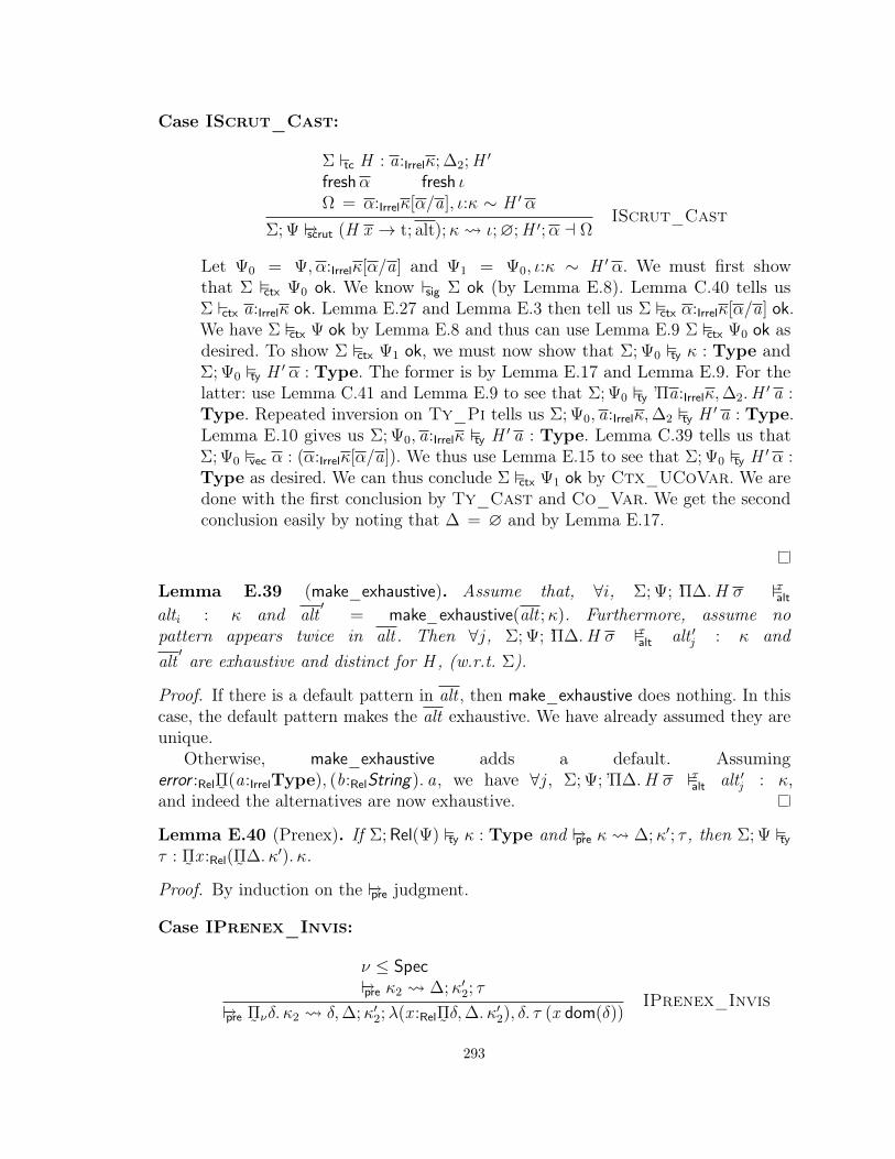
Case IScrut_Cast:

Σ tc H : a:Irrelκ; ∆2;H ′

freshα fresh ιΩ = α:Irrelκ[α/a], ι:κ ∼ H ′ α

Σ; Ψ scrut (H x → t; alt);κ ι;∅;H ′;α a ΩIScrut_Cast

Let Ψ0 = Ψ, α:Irrelκ[α/a] and Ψ1 = Ψ0, ι:κ ∼ H ′ α. We must first showthat Σ ctx Ψ0 ok. We know sig Σ ok (by Lemma E.8). Lemma C.40 tells usΣ ctx a:Irrelκ ok. Lemma E.27 and Lemma E.3 then tell us Σ ctx α:Irrelκ[α/a] ok.We have Σ ctx Ψ ok by Lemma E.8 and thus can use Lemma E.9 Σ ctx Ψ0 ok asdesired. To show Σ ctx Ψ1 ok, we must now show that Σ; Ψ0 ty κ : Type andΣ; Ψ0 ty H ′ α : Type. The former is by Lemma E.17 and Lemma E.9. For thelatter: use Lemma C.41 and Lemma E.9 to see that Σ; Ψ0 ty ’Πa:Irrelκ,∆2.H

′ a :Type. Repeated inversion on Ty_Pi tells us Σ; Ψ0, a:Irrelκ,∆2 ty H ′ a : Type.Lemma E.10 gives us Σ; Ψ0, a:Irrelκ ty H ′ a : Type. Lemma C.39 tells us thatΣ; Ψ0 vec α : (α:Irrelκ[α/a]). We thus use Lemma E.15 to see that Σ; Ψ0 ty H ′ α :Type as desired. We can thus conclude Σ ctx Ψ1 ok by Ctx_UCoVar. We aredone with the first conclusion by Ty_Cast and Co_Var. We get the secondconclusion easily by noting that ∆ = ∅ and by Lemma E.17.

Lemma E.39 (make_exhaustive). Assume that, ∀i, Σ; Ψ; ’Π∆.H σ τaltalti : κ and alt

′= make_exhaustive(alt ;κ). Furthermore, assume no

pattern appears twice in alt . Then ∀j, Σ; Ψ; ’Π∆.H σ τalt alt ′j : κ andalt′are exhaustive and distinct for H , (w.r.t. Σ).

Proof. If there is a default pattern in alt , then make_exhaustive does nothing. In thiscase, the default pattern makes the alt exhaustive. We have already assumed they areunique.

Otherwise, make_exhaustive adds a default. Assumingerror :Rel

˜Π(a:IrrelType), (b:RelString). a, we have ∀j, Σ; Ψ; ’Π∆.H σ τalt alt ′j : κ,

and indeed the alternatives are now exhaustive.

Lemma E.40 (Prenex). If Σ; Rel(Ψ) ty κ : Type and pre κ ∆;κ′; τ , then Σ; Ψ tyτ :

˜Πx :Rel(

˜Π∆. κ′). κ.

Proof. By induction on the pre judgment.

Case IPrenex_Invis:

ν ≤ Specpre κ2 ∆;κ′2; τ

pre˜Πνδ. κ2 δ,∆;κ′2;λ(x :Rel

˜Πδ,∆. κ′2), δ. τ (x dom(δ))

IPrenex_Invis

293

We know Σ; Rel(Ψ) ty˜Πνδ. κ2 : Type. Inversion gives us Σ; Rel(Ψ, δ) ty

κ2 : Type. The induction hypothesis thus tells us that Σ; Ψ, δ ty τ :

˜Πx2:Rel(

˜Π∆. κ′2). κ2. Let Ψ′ = Ψ, x :Rel(

˜Πδ,∆. κ′2), δ. We need Σ ctx Ψ′ ok,

for which we need Σ; Rel(Ψ) ty˜Πδ,∆. κ′2 : Type, which can be proved

by inversions and Ty_Pi. We thus have Σ ctx Ψ′ ok. We now show thatΣ; Ψ′ ty τ (x dom(δ)) : κ2. First, we note that Σ; Ψ′ ty x dom(δ) :

˜Π∆. κ′2 by

the appropriate application rule. (It depends on the relevance of δ.) Thereis no substitution in the kind, because we are applying to dom(δ). ThusΣ; Ψ′ ty τ (x dom(δ)) : κ2[x dom(δ)/x2] by Ty_AppRel. However, we knowx2 # κ2 by Lemma E.11 and so we are done by two uses of Ty_Lam.

Case IPrenex_Vis:

pre κ2 ∆;κ′2; ττ0 = λ(x :Rel

˜Π∆, δ. κ′2), δ. τ (λ∆. x dom(∆) dom(δ))

pre˜ΠReqδ. κ2 ∆;

˜ΠReqδ. κ′2; τ0

IPrenex_Vis

We know Σ; Rel(Ψ) ty˜ΠReqδ. κ2 : Type. Inversion gives us Σ; Rel(Ψ, δ) ty κ2 :

Type. The induction hypothesis then gives us Σ; Ψ, δ ty τ :˜Πx2:Rel(

˜Π∆. κ′2). κ2.

Let Ψ′ = Ψ, x :Rel(˜Π∆, δ. κ′2), δ. We need Σ ctx Ψ′ ok, for which we need

Σ; Rel(Ψ) ty˜Π∆, δ. κ′2 : Type. This can be proved by inversions and Ty_Pi. We

thus have Σ ctx Ψ′ ok. We now show that Σ; Ψ′ ty τ (λ∆. x dom(∆) dom(δ)) : κ2.First, we show that Σ; Ψ′,∆ ty x dom(∆) dom(δ) : κ′2. Once we show thatΣ ctx Ψ′,∆ ok (as can be shown by inversions, Lemma E.8, and LemmaE.9), then this comes directly from the type of x . Thus, we can conclude,by repeated use ofTy_Lam, that Σ; Ψ′ ty λ∆. x dom(∆) dom(δ) :

˜Π∆. κ′2. Ac-

cordingly, Σ; Ψ′ ty τ (λ∆. x dom(∆) dom(δ)) : κ2[(λ∆. x dom(∆) dom(δ))/x2],but the substitution in the kind has no effect by Lemma E.11. We thus haveΣ; Ψ′ ty τ (λ∆. x dom(∆) dom(δ)) : κ2. We are done by several uses of Ty_Lam.

Case IPrenex_NoPi:

pre κ ∅;κ;λx :Relκ. xIPrenex_NoPi

Assuming Σ; Rel(Ψ) ty κ : Type, we must show Σ; Ψ ty λx :Relκ. x :˜Πx :Relκ. κ.

This is true by straightforward application of typing rules.

Lemma E.41 (Subsumption). Assume Σ; Rel(Ψ) ty κ1 : Type and Σ; Rel(Ψ) ty κ2 :Type. If either

1. κ1 ≤∗ κ2 τ a Ω, OR

2. κ1 ≤ κ2 τ a Ω

294

Then Σ; Ψ,Ω ty τ :˜Πx :Relκ1. κ2.

Proof. By mutual induction on the subsumption judgments.

Case ISub_FunRel:

κ3 ≤ κ1 τ1 a Ω1 κ2[τ1 b/a] ≤ κ4 τ2 a Ω2

Ω2 → b:Relκ3 Ω′2; ξτ0 = λx :Rel(Πa:Relκ1. κ2), b:Relκ3. τ2[ξ] (x (τ1 b))

ΠReqa:Relκ1. κ2 ≤∗˜ΠReqb:Relκ3. κ4 τ0 a Ω1,Ω′2

ISub_FunRel

Our assumption says that Σ; Rel(Ψ) ty Πa:Relκ1. κ2 : Type and Σ; Rel(Ψ) ty

˜Πa:Relκ3. κ4 : Type. Inversion of Ty_Pi tells us the following:

• Σ; Rel(Ψ) ty κ1 : Type

• Σ; Rel(Ψ), a:Relκ1 ty κ2 : Type

• Σ; Rel(Ψ) ty κ3 : Type

• Σ; Rel(Ψ), b:Relκ3 ty κ4 : Type

The induction hypothesis then tells us Σ; Ψ,Ω1 ty τ1 :˜Πx1:Relκ3. κ1. Lemma E.9

gives us Σ; Rel(Ψ,Ω1), b:Relκ3, a:Relκ1 ty κ2 : Type. Rule Ty_AppRel tells usΣ; Ψ,Ω1, b:Relκ3 ty τ1 b : κ1[b/x ], but Lemma E.11 tells us that the substitution inthe kind has no effect. We can thus use Lemma E.13 to get Σ; Rel(Ψ,Ω1), b:Relκ3 tyκ2[τ1 b/a] : Type. Now, we can use the induction hypothesis again to getΣ; Ψ,Ω1, b:Relκ3,Ω2 ty τ2 :

˜Πx2:Relκ2[τ1 b/a]. κ4. Lemma E.35 tells us now that

Σ; Ψ,Ω1,Ω′2, b:Relκ3 ty τ2[ξ] : (

˜Πx2:Relκ2[τ1 b/a]. κ4)[ξ], but Lemma E.34 tells us

the [ξ] in the kind has no effect. Let

Ψ′ = Ψ,Ω1,Ω′2, x :Rel(Πa:Relκ1. κ2), b:Relκ3.

To show Σ ctx Ψ′ ok, we need only show that Σ; Rel(Ψ,Ω1),Ω′2 ty Πa:Relκ1. κ2 :Type (noting that Lemma E.35 and Lemma E.8 imply Σ ctx Ψ,Ω1,Ω

′2 ok),

but this is true by Lemma E.9. We must now show Σ; Ψ′ ty τ2[ξ] (x (τ1 b)) : κ4.We’ve already ascertained that Σ; Ψ′ ty τ1 b : κ1. We see that Σ; Ψ′ ty x (τ1 b) :κ2[τ1 b/a]. Thus Σ; Ψ′ ty τ2[ξ] (x (τ1 b)) : κ4[x (τ1 b)/x2], but Lemma E.11 tellsus that the substitution in the kind has no effect. We are thus done by two usesof Ty_Lam.

Case ISub_FunIrrelRel: Similar to previous case. Note that b can be usedirrelevantly even though it is bound relevantly. The opposite way would notwork.

Case ISub_FunIrrel: Similar to previous case.

295

Case ISub_Unify:

fresh ι

τ1 ≤∗ τ2 λx :Relτ1. (x B ι) a ι:τ1 ∼ τ2

ISub_Unify

We must show that Σ; Ψ, ι:τ1 ∼ τ2 ty λx :Relτ1. (x B ι) :˜Πx :Relτ1. τ2. Our last step

will be Ty_Lam and thus we must show Σ; Ψ, ι:τ1 ∼ τ2, x :Relτ1 ty x B ι : τ2,for which we only need show that Σ ctx Ψ, ι:τ1 ∼ τ2 ok, for which we only needshow that Σ; Rel(Ψ) ty τ1 : Type and Σ; Rel(Ψ) ty τ2 : Type, which we knowby assumption. We are done.

Case ISub_DeepSkol:

pre κ2 ∆;κ′2; τ1

Specinst κ1 ψ;κ′1 a Ω1

κ′1 ≤∗ κ′2 τ2 a Ω2

Ω1,Ω2 → ∆ Ω′; ξ

κ1 ≤ κ2 λx :Relκ1. τ1 (λ∆. τ2[ξ] (x ψ[ξ])) a Ω′ISub_DeepSkol

We must show Σ; Ψ,Ω′ ty λx :Relκ1. τ1 (λ∆. τ2[ξ] (x ψ[ξ])) :˜Πx :Relκ1. κ2. The last

step will be Ty_Lam, so we must show Σ; Ψ,Ω′, x :Relκ1 ty τ1 (λ∆. τ2[ξ] (x ψ[ξ])) :κ2. From Σ; Rel(Ψ) ty κ1 : Type, we can use Ctx_TyVar to see Σ ctxΨ, x :Relκ1 ok. Thus Σ; Ψ, x :Relκ1 ty x : κ1. Lemma E.36 then tells usthat Σ; Ψ, x :Relκ1,Ω1 ty x ψ : κ′1. We then know (by Lemma E.17) thatΣ; Rel(Ψ, x :Relκ1,Ω1) ty κ′1 : Type. Lemma E.40 tells us that Σ; Ψ ty τ1 :

˜Πx1:Rel(

˜Π∆. κ′2). κ2. Lemma E.17 and inversion gives Σ; Rel(Ψ,∆) ty κ′2 : Type.

We can then use the induction hypothesis with context Ψ, x :Relκ1,∆,Ω1 (knownwell-formed by Lemma E.9) to get Σ; Ψ, x :Relκ1,∆,Ω1,Ω2 ty τ2 :

˜Πx2:Relκ

′1. κ′2.

Lemma E.35 shows that Σ; Ψ, x :Relκ1,Ω′,∆ ty τ2[ξ] : (

˜Πx2:Relκ

′1. κ′2)[ξ]. The

kind can be rewritten to˜Πx2:Rel(κ

′1[ξ]). κ

′2[ξ] but Lemma E.34 tells us that

κ′2[ξ] = κ′2. We established earlier that Σ; Ψ, x :Relκ1,Ω1 ty x ψ : κ′1. We canweaken this to Σ; Ψ, x :Relκ1,∆,Ω1,Ω2 ty x ψ : κ′1 and then use Lemma E.35to get Σ; Ψ, x :Relκ1,Ω

′,∆ ty (x ψ)[ξ] : κ′1[ξ]. We know that x [ξ] = x be-cause x is just a non-unification variable. Rule Ty_AppRel thus gives usΣ; Ψ, x :Relκ1,Ω

′,∆ ty τ2[ξ] (x ψ[ξ]) : κ′2[x ψ[ξ]/x2] but Lemma E.11 tells us thatthe substitution in the kind has no effect. We now use Ty_Lam (repeatedly)to see Σ; Ψ, x :Relκ1,Ω

′ ty λ∆. τ2[ξ] (x ψ[ξ]) :˜Π∆. κ′2. Thus Ty_AppRel tells us

Σ; Ψ, x :Relκ1,Ω′ ty τ1 (λ∆. τ2[ξ] (x ψ[ξ])) : κ2[(λ∆. τ2[ξ] (x ψ[ξ]))/x1], but Lemma

E.11 tells us that the substitution in the kind has no effect. We only need toreshuffle the context; in other words, we must now show Σ ctx Ψ,Ω′, x :Relκ1 okto be done. For this to hold, we need to know that none of Ω′ depend on x . First,note that x is local to rule ISub_DeepSkol. We see that ∆ is produced by prewith no mention of x , Ω1 is produced by inst with no mention of x , and Ω2 is

296

produced by ≤∗ with no mention of x . Therefore, x is not mentioned in any ofthese, and we are done.

Lemma E.42 (Type elaboration is sound).

1. If any of the following:

(a) Σ ctx Ψ ok and Σ; Ψ ty t τ : κ a Ω, OR(b) Σ ctx Ψ ok and Σ; Ψ ∗

ty t τ : κ a Ω, OR(c) Σ; Rel(Ψ) ty κ : Type and Σ; Ψ ty t : κ τ a Ω, OR(d) Σ; Rel(Ψ) ty κ : Type and Σ; Ψ ∗

ty t : κ τ a Ω

Then Σ; Ψ,Ω ty τ : κ.

2. If Σ ctx Ψ ok and Σ; Ψ pt s σ a Ω, then Σ; Rel(Ψ,Ω) ty σ : Type.

3. If Σ; Ψ ty τ1 : Πνa:ρκ1. κ2 and Σ; Ψ; ρ ∗arg t2 : κ1 ψ2; τ2 a Ω, then Σ; Ψ,Ω tyτ1 ψ2 : κ2[τ2/a].

4. If Σ; Rel(Ψ) ty κ : Type, Σ; Ψ ty τ0 : ’Π∆.H τ , Σ; Rel(Ψ) ty H τ : Type, andΣ; Ψ; ’Π∆.H τ ; τ0 alt alt : κ alt a Ω, then Σ; Ψ,Ω; ’Π∆.H τ τ0alt alt : κ.

5. If Σ; Rel(Ψ) ty κ : Type, Σ; Ψ ty τ0 : ’Π∆.H τ , Σ; Rel(Ψ) ty H τ : Type, andΣ; Ψ;κ0; τ0 altc alt : κ alt a Ω, then Σ; Ψ,Ω;κ0

τ0alt alt : κ.

6. If Σ ctx Ψ ok and Σ; Ψ q qvar a : κ; ν a Ω, then Σ; Rel(Ψ,Ω) ty κ : Type.

7. If Σ ctx Ψ ok and Σ; Ψ aq aqvar a : κ a Ω, then Σ; Rel(Ψ,Ω) ty κ : Type.

8. If Σ; Ψ ty τ0 : κ and Σ; Ψ aq aqvar : κ a : κ′; x .τ a Ω, then Σ; Ψ,Ω ty τ [τ0/x ] :κ′.

Proof. Proceed by induction on the structure of the type inference derivation.

Case ITy_Inst:

Σ; Ψ ∗ty t τ : κ a Ω1

Specinst κ ψ;κ′ a Ω2

Σ; Ψ ty t τ ψ : κ′ a Ω1,Ω2

ITy_Inst

The induction hypothesis gives us Σ; Ψ,Ω1 ty τ : κ. Lemma E.36 then gives usΣ; Ψ,Ω1,Ω2 ty τ ψ : κ′ as desired.

Case ITy_Var: By Ty_Var and Lemma E.36.

297

Case ITy_App:

Σ; Ψ ty t1 τ1 : κ0 a Ω1

fun κ0; Rel γ; Π; a; ρ;κ1;κ2 a Ω2

Σ; Ψ,Ω1,Ω2; ρ ∗arg t2 : κ1 ψ2; τ2 a Ω3

Σ; Ψ ∗ty t1 t2 (τ1 B γ)ψ2 : κ2[τ2/a] a Ω1,Ω2,Ω3

ITy_App

The induction hypothesis tells us that Σ; Ψ,Ω1 ty τ1 : κ0. Thus Σ; Rel(Ψ,Ω1) tyκ0 : Type by Lemma E.17. Lemma E.37 tells us that Σ; Rel(Ψ,Ω1,Ω2) co γ :κ0 ∼ ΠReqa:ρκ1. κ2. Rule Ty_Cast gives us Σ; Ψ,Ω1,Ω2 ty τ1Bγ : ΠReqa:ρκ1. κ2.Another use of the induction hypothesis (for the ∗arg premise) gives us our desiredoutcome.

Case ITy_AppSpec: By induction.

Case ITy_Annot: By induction.

Case ITy_Case:

Σ; Ψ ty t0 τ0 : κ0 a Ω0

Σ; Ψ,Ω0 scrut alt;κ0 γ; ∆;H ′; τ a Ω′0freshα Ω′ = Ω0,Ω

′0, α:IrrelType

∀i , Σ; Ψ,Ω′; ’Π∆.H ′ τ ; τ0 B γ alt alti : α alti a Ωi

alt′

= make_exhaustive(alt ;κ)

Σ; Ψ ∗ty case t0 of alt caseα (τ0 B γ) of alt

′: α a Ω′,Ω

ITy_Case

The induction hypothesis tells us that Σ; Ψ,Ω0 ty τ0 : κ0. Lemma E.38 tellsus that Σ; Ψ,Ω0,Ω

′0 ty τ0 B γ : ’Π∆.H ′ τ and Σ; Rel(Ψ,Ω0,Ω

′0) ty H

′ τ : Type.Rule Ctx_UTyVar gives us Σ ctx Ω′ ok. The induction hypothesis (for alt)tells us that, ∀i, Σ; Ψ,Ω′,Ωi ; ’Π∆.H ′ τ τ0Bγalt alti : α. Lemma E.39 then tells usthat alt ′ are well-formed and exhaustive. Lemma E.9 (and Lemma E.8 on the altjudgments) allows us to combine all the Ωi into Ω. We are done by Ty_Case.

Case ITy_Lam:

Σ; Ψ q qvar a : κ1; ν a Ω1

Σ; Ψ,Ω1, a:Relκ1 ∗ty t τ : κ2 a Ω2

Ω2 → a:Relκ1 Ω′2; ξ

Σ; Ψ ∗ty λqvar. t λa:Relκ1. (τ [ξ]) :

˜Πνa:Relκ1. (κ2[ξ]) a Ω1,Ω′2

ITy_Lam

The induction hypothesis (on q) tells us that Σ; Rel(Ψ,Ω1) ty κ1 : Type.Thus Σ ctx Ψ,Ω1, a:Relκ1 ok and we can use the induction hypothesis to getΣ; Ψ,Ω1, a:Relκ1,Ω2 ty τ : κ2. By Lemma E.35, we get Σ; Ψ,Ω1,Ω

′2, a:Relκ1 ty

τ [ξ] : κ2[ξ] and thus Σ; Ψ,Ω1,Ω′2 ty λa:Relκ1. (τ [ξ]) :

˜Πνa:Relκ1. (κ2[ξ]) as desired.

Case ITy_LamIrrel: Like previous case.

298

Case ITy_Arrow: By induction and Lemma E.9

Case ITy_MArrow: By induction and Lemma E.9

Case ITy_Fix:

Σ; Ψ ty t τ : κ a Ω1

fun κ; Rel γ;˜Π; a; Rel;κ1;κ2 a Ω2

Σ; Rel(Ψ,Ω1,Ω2) ty κ2 : Typefresh ι Ω = Ω1,Ω2, ι:κ2 ∼ κ1

Σ; Ψ ∗ty fix t fix (τ B (γ #

˜Πa:Rel〈κ1〉. ι)) : κ1 a Ω

ITy_Fix

The induction hypothesis gives us Σ; Ψ,Ω1 ty τ : κ and thus Σ; Rel(Ψ,Ω1) tyκ : Type by Lemma E.17. Lemma E.37 gives us Σ; Rel(Ψ,Ω1,Ω2) co γ : κ ∼

˜ΠReqa:Relκ1. κ2 and then Ty_Cast tells us Σ; Ψ,Ω1,Ω2 ty τBγ :

˜ΠReqa:Relκ1. κ2.

Thus, Lemma E.8 tells us Σ ctx Ψ,Ω1,Ω2 ok. In order to prove Σ ctx Ω ok, wemust show Σ; Rel(Ψ,Ω1,Ω2) ty κ2 : Type and Σ; Rel(Ψ,Ω1,Ω2) ty κ1 : Type.The first of these is a premise to ITy_Fix. To get the second, we use LemmaE.17 to get Σ; Rel(Ψ,Ω1,Ω2) ty

˜ΠReqa:Relκ1. κ2 : Type and then invert. We can

conclude Σ ctx Ω ok by Ctx_UCoVar.

Inversion on Σ; Ψ,Ω1,Ω2 ty τ B γ :˜ΠReqa:Relκ1. κ2 tells us that Σ; Rel(Ψ,Ω) co

γ : κ ∼˜ΠReqa:Relκ1. κ2. We can further see (by Co_PiTy) that Σ; Rel(Ψ,Ω) co

˜Πa:Rel〈κ1〉. ι : (

˜Πa:Relκ1. κ2) ∼ (

˜Πa:Relκ1. (κ1[aBsym 〈κ1〉/a])) However, because

a # κ1 (by Lemma E.11), that last substitution has no effect, and so weconclude Σ; Rel(Ψ,Ω) co

˜Πa:Rel〈κ1〉. ι : (

˜Πa:Relκ1. κ2) ∼ (

˜Πa:Relκ1. κ1) and thus

Σ; Ψ,Ω ty τB(γ#˜Πa:Rel〈κ1〉. ι) :

˜Πa:Relκ1. κ1. Finally, Ty_Fix gives us Σ; Ψ,Ω ty

fix (τ B (γ #˜Πa:Rel〈κ1〉. ι)) : κ1 as desired.

Case ITy_Let:

Σ; Ψ ∗ty t1 τ1 : κ1 a Ω

Σ; Ψ,Ω, x :Relκ1 ∗ty t2 τ2 : κ2 a Ω2

Ω2 → x :Relκ1 Ω′2; ξ

Σ; Ψ ∗ty let x := t1 in t2 (λx :Relκ1. (τ2[ξ])) τ1 : κ2[ξ][τ1/x ] a Ω,Ω′2

ITy_Let

The induction hypothesis gives us Σ; Ψ,Ω ty τ1 : κ1. Lemma E.17 tells usΣ; Rel(Ψ,Ω) ty κ1 : Type and thus that Σ ctx Ψ,Ω, x :Relκ1 ok. Another useof the induction hypothesis gives us Σ; Ψ,Ω, x :Relκ1,Ω2 ty τ2 : κ2. LemmaE.35 then gives us Σ; Ψ,Ω,Ω′2, x :Relκ1 ty τ2[ξ] : κ2[ξ] and thus Σ; Ψ,Ω,Ω′2 tyλx :Relκ1. (τ2[ξ]) :

˜Πx :Relκ1. (κ2[ξ]) Rule Ty_AppRel gives us Σ; Ψ,Ω,Ω′2 ty

(λx :Relκ1. (τ2[ξ])) τ1 : κ2[ξ][τ1/x ] as desired.

Case ITyC_Case: Similar to the case for ITy_Case. The only differences arethe definition of Ω′ (which is simpler in this case) and the use of altc in place ofalt. Both alt and altc are proven sound via the induction hypothesis.

299

Case ITyC_LamDep:

fun κ; Rel γ;˜Π; a; Rel;κ1;κ2 a Ω0

¬(a # κ2)Σ; Rel(Ψ) pt s κ′1 a Ω1

Ω = Ω0,Ω1, ι:κ1 ∼ κ′1Σ; Ψ,Ω, b:Relκ

′1∗ty t : κ2[b B sym ι/a] τ a Ω2

Ω2 → b:Relκ′1 Ω′2; ξ

η = κ2[(a B ι)B sym ι/a] ≈〈Type〉 κ2

τ0 = (λa:Relκ1. (τ [ξ][a B ι/b]B η))B sym γ

Σ; Ψ ty λ(a :: s). t : κ τ0 a Ω,Ω′2ITyC_LamDep

We have assumed Σ; Rel(Ψ) ty κ : Type and thus can use Lemma E.37 to getΣ; Rel(Ψ,Ω0) co γ : κ ∼

˜ΠReqa:Relκ1. κ2. (The ¬(a # κ2) premise is not used in

this rule; it is used to filter out which cases are handled in the next one.) ByLemma E.8, we have Σ ctx Rel(Ψ) ok and thus can use the induction hypothesis toget Σ; Rel(Ψ,Ω1) ty κ′1 : Type. We must now prove that Σ; Rel(Ψ,Ω), b:Relκ

′1 ty

κ2[b B sym ι/a] : Type. First, we prove that Σ ctx Rel(Ψ,Ω), b:Relκ′1 ok. For

this, it is left to prove only that Σ; Rel(Ψ,Ω0,Ω1) ty κ1 : Type. This we canget from Lemma E.18, inversion of Ty_Pi, and Lemma E.4. The inversionof Ty_Pi also tells us that Σ; Rel(Ψ,Ω0), a:Relκ1 ty κ2 : Type. Lemma E.9allows us to weaken this to Σ; Rel(Ψ,Ω), b:Relκ

′1, a:Relκ1 ty κ2 : Type. We can

see that Σ; Rel(Ψ,Ω), b:Relκ′1 ty b B sym ι : κ1. We thus use Lemma E.13 to

get Σ; Rel(Ψ,Ω), b:Relκ′1 ty κ2[b B sym ι/a] : Type as desired. We then use the

induction hypothesis to get Σ; Ψ,Ω, b:Relκ′1,Ω2 ty τ : κ2[b B sym ι/a]. Lemma

E.35 allows us to rewrite this to Σ; Ψ,Ω,Ω′2, b:Relκ′1 ty τ [ξ] : κ2[b B sym ι/a][ξ],

but Lemma E.34 tells us the [ξ] in the kind has no effect. Lemma E.9 allowsus to weaken this to Σ; Ψ,Ω,Ω′2, a:Relκ1, b:Relκ

′1 ty τ [ξ] : κ2[b B sym ι/a]. We

can see that Σ; Ψ,Ω,Ω′2, a:Relκ1 ty a B ι : κ′1 and thus we can use Lemma E.13to get Σ; Ψ,Ω,Ω′2, a:Relκ1 ty τ [ξ][a B ι/b] : κ2[b B sym ι/a][a B ι/b]. Inliningsubstitutions, we can rewrite the kind to κ2[(a B ι) B sym ι/a]. We can thensee that Σ; Ψ,Ω,Ω′2, a:Relκ1 ty τ [ξ][a B ι/b] B η : κ2 and by Ty_Lam thatΣ; Ψ,Ω,Ω′2 ty λa:Relκ1. (τ [ξ][a B ι/b] B η) :

˜Πa:Relκ1. κ2. A use of Ty_Cast

gives us Σ; Ψ,Ω,Ω′2 ty (λa:Relκ1. (τ [ξ][a B ι/b]B η))B sym γ : κ as desired.

Case ITyC_Lam:

fun κ; Rel γ;˜Π; a; Rel;κ1;κ2 a Ω0

Σ; Ψ aq aqvar : κ1 b : κ′1; x .τ1 a Ω1

Σ; Ψ,Ω0,Ω1, b:Relκ′1∗ty t : κ2 τ a Ω2

Ω2 → b:Relκ′1 Ω′2; ξ

Ω′ = Ω0,Ω1,Ω′2

Σ; Ψ ty λaqvar. t : κ (λa:Relκ1. τ [ξ][τ1[a/x ]/b])B sym γ a Ω′ITyC_Lam

300

Lemma E.37 tells us Σ; Rel(Ψ,Ω0) co γ : κ ∼˜ΠReqa:Relκ1. κ2. Lemma E.18 and

inversions tell us Σ; Rel(Ψ,Ω0) ty κ1 : Type and Σ; Rel(Ψ,Ω0), a:Relκ1 ty κ2 :Type. We can conclude Σ ctx Rel(Ψ,Ω0), a:Relκ1 ok and thus (using LemmaE.28) Σ; Ψ,Ω0, a:Relκ1 ty a : κ1. The induction hypothesis on aq then tells usΣ; Ψ,Ω0, a:Relκ1,Ω1 ty τ1[a/x ] : κ′1. We can see by the construction of Ω1 and κ′1that a # Ω1 and a # κ′1. Because we are in rule ITyC_Lam, it means thatITyC_LamDep does not apply. This can be for one of two reasons, and thuswe now have two cases:

Case aqvar = a (unannotated binder): In this case, we see (by IAQ-VarC_Var) that κ′1 = κ1. We can choose a = b by the α-renaming.Thus, Σ; Rel(Ψ,Ω0), b:Relκ

′1 ty κ2 : Type.

Case a # κ2: We now use Lemma E.10 to get Σ; Rel(Ψ,Ω0) ty κ2 : Type.

Regardless of which case above we are in, we now must prove Σ ctxΨ,Ω0,Ω1, b:Relκ

′1 ok. To do this, we must show only that Σ; Rel(Ψ,Ω0,Ω1) ty

κ′1 : Type, which comes from Lemma E.17 and Lemma E.10. We can then useLemma E.9 to get Σ; Rel(Ψ,Ω0,Ω1), b:Relκ

′1 ty κ2 : Type. The induction hypoth-

esis now applies to get Σ; Ψ,Ω0,Ω1, b:Relκ′1,Ω2 ty τ : κ2. Lemma E.35 tells us

Σ; Ψ,Ω0,Ω1,Ω′2, b:Relκ

′1 ty τ [ξ] : κ2[ξ], but Lemma E.34 tells us the [ξ] in the kind

has no effect. Lemma E.9 gives us Σ; Ψ,Ω0, a:Relκ1,Ω1,Ω′2, b:Relκ

′1 ty τ [ξ] : κ2.

We can thus use Lemma E.13 to get Σ; Ψ,Ω0, a:Relκ1,Ω1,Ω′2 ty τ [ξ][τ1[a/x ]/b] :

κ2[τ1[a/x ]/b], but Lemma E.11 tells us the substitution in the kind has no effect.Noting that, by analysis stemming from our two cases previously, a # Ω′2,we can reshuffle the context to be Ψ,Ω0,Ω1,Ω

′2, a:Relκ1 and thus conclude

Σ; Ψ,Ω0,Ω1,Ω′2 ty λa:Relκ1. τ [ξ][τ1[a/x ]/b] :

˜Πa:Relκ1. κ2. Thus Ty_Cast gives

us Σ; Ψ,Ω0,Ω1,Ω′2 ty (λa:Relκ1. τ [ξ][τ1[a/x ]/b])B sym γ : κ as desired.

Case ITyC_LamIrrelDep: Like case for ITyC_LamDep.

Case ITyC_LamIrrel: Like case for ITyC_Lam.

Case ITyC_Fix:

Σ; Ψ ty t :˜ΠReqa:Relκ. κ τ a Ω

Σ; Ψ ty fix t : κ fix τ a ΩITyC_Fix

We know Σ; Rel(Ψ) ty κ : Type. We can thus conclude by Ty_Pi thatΣ; Rel(Ψ) ty

˜Πa:Relκ. κ : Type. We thus use the induction hypothesis to get

Σ; Ψ,Ω ty τ :˜Πa:Relκ. κ. Thus we are done by Ty_Fix.

301

Case ITyC_Infer:

Σ; Ψ ∗ty t τ : κ1 a Ω

pre κ2 ∆;κ′2; τ2

Ω → ∆ Ω′; ξ1

κ1[ξ1] ≤∗ κ′2 τ ′2 a Ω2

Ω2 → ∆ Ω′2; ξ2

Σ; Ψ ty t : κ2 τ2 (λ∆. τ ′2[ξ2] τ [ξ1]) a Ω′,Ω′2ITyC_Infer

The induction hypothesis tells us that Σ; Ψ,Ω ty τ : κ1. We have assumedΣ; Rel(Ψ) ty κ2 : Type. We can thus use Lemma E.40 to get Σ; Ψ ty τ2 :

˜Πx :Rel(

˜Π∆. κ′2). κ2. Lemma E.17 and inversion gives us Σ; Rel(Ψ,∆) ty κ′2 : Type

and thus Lemma E.8 and Lemma E.28 give us Σ ctx Ψ,∆ ok. We can thususe Lemma E.9 to get Σ; Ψ,∆,Ω ty τ : κ1 and then Lemma E.35 to getΣ; Ψ,Ω′,∆ ty τ [ξ1] : κ1[ξ1]. Lemma E.17 tells us Σ; Rel(Ψ,Ω′,∆) ty κ1[ξ1] :Type and Lemma E.9 tells us Σ; Rel(Ψ,Ω′,∆) ty κ′2 : Type. We can thus useLemma E.41 to get Σ; Ψ,Ω′,∆,Ω2 ty τ ′2 :

˜Πx :Rel(κ1[ξ1]). κ

′2. Lemma E.35 then

tells us Σ; Ψ,Ω′,Ω′2,∆ ty τ′2[ξ2] : (

˜Πx :Rel(κ1[ξ1]). κ

′2)[ξ2], but Lemma E.34 tells

us that the [ξ2] in the kind has no effect (because neither κ′2 nor κ1 nor ξ1

can mention anything bound in Ω2). We thus have Σ; Ψ,Ω′,Ω′2,∆ ty τ′2[ξ2] :

˜Πx :Rel(κ1[ξ1]). κ

′2. Ty_AppRel (with Lemma E.9) tells us Σ; Ψ,Ω′,Ω′2,∆ ty

τ ′2[ξ2] τ [ξ1] : κ′2[τ [ξ1]/x ] but Lemma E.11 tells us that the substitution in the kindhas no effect. Multiple uses of Ty_Lam gives us Σ; Ψ,Ω′,Ω′2 ty λ∆. τ ′2[ξ2] τ [ξ1] :

˜Π∆. κ′2. Yet another use of Lemma E.9 and Ty_AppRel gives us Σ; Ψ,Ω′,Ω′2 tyτ2 (λ∆. τ ′2[ξ2] τ [ξ1]) : κ2[λ∆. τ ′2[ξ2] τ [ξ1]/x ], where Lemma E.11 tells us that thesubstitution in the kind has no effect. We are thus done.

Invisible λ/Λ cases: Like corresponding visible λ/Λ cases. Note that the differencebetween the ty and ∗

ty checking judgments is relevant for user-facing issues oftype inference (e.g., principal types), not the soundness we are proving here.

Case ITyC_Let: Similar to case for ITy_Let. The only difference is that theexpected type is propagated down.

Case ITyC_Skol:

ν ≤ SpecΣ; Ψ, $a:ρκ1 ∗ty t : κ2 τ a ΩΩ → $a:ρκ1 Ω′; ξ

Σ; Ψ ∗ty t :

˜Πν$a:ρκ1. κ2 λ$a:ρκ1. τ [ξ] a Ω′

ITyC_Skol

We have assumed Σ; Rel(Ψ) ty˜Πν$a:ρκ1. κ2 : Type. Inversion gives us

Σ; Rel(Ψ), $a:Relκ1 ty κ2 : Type, and we can thus use the induction hypothesis toget Σ; Ψ, $a:ρκ1,Ω ty τ : κ2. Lemma E.35 tells us Σ; Ψ,Ω′, $a:ρκ1 ty τ [ξ] : κ2[ξ],but Lemma E.34 tells us that the [ξ] in the kind has no effect. We can thus

302

conclude Σ; Ψ,Ω′ ty λ$a:ρκ1. (τ [ξ]) :˜Πν$a:ρκ1. κ2 as desired.

Case ITyC_Otherwise: By induction.

Case IPtC_Pi:

pi quant Π; ρΣ; Ψ q qvar a : κ; ν a ΩΣ; Ψ,Ω, a:ρκ pt s σ a Ω2

Ω2 → a:ρκ Ω′2; ξ

Σ; Ψ pt ∀ qvar. s Πνa:ρκ. (σ[ξ]) a Ω,Ω′2IPtC_Pi

The induction hypothesis (on q) tells us Σ; Rel(Ψ,Ω) ty κ : Type. Thus Σ ctxRel(Ψ,Ω, a:ρκ) ok and we can use the induction hypothesis (on pt) to getΣ; Rel(Ψ,Ω, a:ρκ,Ω2) ty σ : Type. Lemma E.35 gives us Σ; Rel(Ψ,Ω,Ω′2, a:ρκ) tyσ[ξ] : Type and thus Σ; Rel(Ψ,Ω,Ω′2) ty

˜Πa:ρκ. (σ[ξ]) : Type as desired.

Case IPtC_Constrained:

Σ; Ψ ty t : Type τ a Ω1

Σ; Ψ,Ω1, $a:Relτ pt s σ a Ω2

Ω2 → $a:Relτ Ω′2; ξ

Σ; Ψ pt t⇒ s ˜ΠInf$a:Relτ. (σ[ξ]) a Ω1,Ω′2

IPtC_Constrained

Lemma C.38, Lemma E.9 and Lemma E.3 tell us Σ; Rel(Ψ) ty Type : Typeand thus we can use the induction hypothesis on ty to get Σ; Ψ,Ω1 ty τ : Type.We thus have Σ ctx Ψ,Ω1, $a:Relτ ok and can use the induction hypothe-sis on pt to get Σ; Rel(Ψ,Ω1, $a:Relτ,Ω2) ty σ : Type. Lemma E.35 givesus Σ; Rel(Ψ,Ω1,Ω

′2, $a:Relτ) ty σ[ξ] : Type and thus Σ; Rel(Ψ,Ω1,Ω

′2) ty

˜ΠInf$a:Relτ. (σ[ξ]) : Type as desired.

Case IPtC_Mono: By induction.

Case IArg_Rel: By induction and straightforward use of typing rules.

Case IArg_Irrel: By induction and straightforward use of typing rules.

Case IAlt_Con:

Σ tc H : ∆1; ∆2;H ′ ∆3,∆4 = ∆2[τ/dom(∆1)]dom(∆3) = x dom(∆4) = dom(∆′)matchdom(∆3)(types(∆4); types(∆′)) = Just θΣ; Ψ,∆3 ty t : κ τ a ΩΩ → ∆3 Ω′; ξ∆′3 = ∆3, c:τ0 ∼ Hτ x

Σ; Ψ; ’Π∆′.H ′ τ ; τ0 alt H x → t : κ H → λ∆′3. (τ [ξ]) a Ω′IAlt_Con

We wish to prove Σ; Ψ,Ω′; ’Π∆′.H ′ τ τ0alt H → λ∆3, (c:τ0 ∼ Hτ x ). (τ [ξ]) : κ,

303

given the premises above along with

• Σ; Rel(Ψ) ty κ : Type

• Σ; Ψ ty τ0 : ’Π∆′.H ′ τ

• Σ; Rel(Ψ) ty H ′ τ : Type

We will use Alt_Match. This requires the following:

Σ tc H : ∆1; ∆2;H ′: This is a premise above.∆3,∆4 = ∆2[τ/dom(∆1)]: This is a premise above.dom(∆4) = dom(∆′): This is a premise above.matchdom(∆3)(types(∆4); types(∆′)) = Just θ: This is a premise above.Σ; Ψ,Ω′ ty λ∆3, (c:τ0 ∼ Hτ x ). (τ [ξ]) : ?Π∆3, c:τ0 ∼ Hτ dom(∆3). κ: Let Ψ′ =

Ψ,Ω′,∆3, c:τ0 ∼ Hτ x . We must show only that Σ; Ψ′ ty τ [ξ] : κ. (Notethat dom(∆3) = x , which is the one discrepancy between the quantifiedcontexts above.) To use the induction hypothesis on ty, we must showΣ; Rel(Ψ,∆3) ty κ : Type, which means we must show only that Σ ctxΨ,∆3 ok and then use Lemma E.9. Lemma C.40 gives us Σ ctx ∆1,∆2 okand by Lemma E.3, Σ ctx ∆1,∆2 ok. Lemma C.77 gives us Σ tc H ′ :∅; Rel(∆1); Type. We know Σ; Rel(Ψ) ty H ′ τ : Type. By Lemma C.42(easily updated to use judgments), we can see that Σ; Rel(Ψ) vec τ :Rel(∆1) and thus Lemma E.15 tells us Σ ctx ∆2[τ/dom(∆1)] ok and byLemma E.8 and Lemma E.9, Σ ctx Ψ,∆3 ok as desired. We have concludedthat Σ; Rel(Ψ,∆3) ty κ : Type and so can use the induction hypothesisto get Σ; Ψ,∆3,Ω ty τ : κ. Lemma E.35 tells us Σ; Ψ,Ω′,∆3 ty τ [ξ] : κ[ξ],but Lemma E.34 tells us that the [ξ] in the conclusion has no effect. Thelast step here is to use weakening to add the binding for c to the context.This requires proving only that Σ; Rel(Ψ,Ω′,∆3) ty Hτ x : ’Π∆4.H

′ τ . Wecan see that Σ; Rel(Ψ,Ω′,∆3) ty Hτ : ’Π∆3,∆4.H

′ τ by Ty_Con. We arethus done by Lemma C.31 (easily updated for judgments).

Case IAlt_Default: By induction and Alt_Default.

Case IAltC_Con: This case is identical to that for IAlt_Con. The difference isthe assumptions that can be made when solving for the unification variables inΩ, which does not affect the course of this proof.

Case IAltC_Default: Similar to the case for IAlt_Default.

Case IQVar_Req: By induction.

Case IQVar_Spec: By induction.

Case IAQVar_Var:

fresh β

Σ; Ψ aq a a : β a β:IrrelTypeIAQVar_Var

304

We must show only that Σ; Rel(Ψ), β:RelType ty β : Type. This is true byTy_UVar.

Case IAQVar_Annot: By induction.

Case IAQVarC_Var:

Σ; Ψ aq a : κ a : κ; x .x a ∅IAQVarC_Var

Given Σ; Ψ ty τ0 : κ, we must show Σ; Ψ ty x [τ0/x ] : κ. By assumption.

Case IAQVarC_Annot:

Σ; Rel(Ψ) pt s σ a Ω1

κ ≤ σ τ a Ω2

Σ; Ψ aq (a :: s) : κ a : σ; x .τ x a Ω1,Ω2

IAQVarC_Annot

Given Σ; Ψ ty τ0 : κ, we must show Σ; Ψ,Ω1,Ω2 ty (τ x )[τ0/x ] : σ, which can berewritten to Σ; Ψ,Ω1,Ω2 ty τ τ0 : σ. We know Σ ctx Ψ ok by Lemma E.8. Theinduction hypothesis then tells us Σ; Rel(Ψ,Ω1) ty σ : Type. Lemma E.17 tellsus Σ; Rel(Ψ) ty κ : Type. We can thus use Lemma E.41 to get Σ; Ψ,Ω1,Ω2 ty τ :

˜Πx :Relκ. σ. Rule Ty_AppRel gives us Σ; Ψ,Ω1,Ω2 ty τ τ0 : σ[τ0/x ], but LemmaE.11 tells us that the substitution in the kind has no effect. We are done.

Lemma E.43 (Declarations). If Σ ctx Γ ok and Σ; Γ decl decl x : κ := τ , thendom(decl) = x and Σ; Γ ty τ : κ.

Proof. By case analysis on the type inference judgment.

Case IDecl_Synthesize:

Σ; Γ ty t τ : κ a ΩΣ; Γ solv Ω ∆; Θτ ′ = λ∆. (τ [Θ]) κ′ =

˜ΠInf∆. (κ[Θ])

Σ; Γ decl x := t x : κ′ := τ ′IDecl_Synthesize

By Lemma E.3, we have Σ ctx Γ ok. We then use Lemma E.42 to get Σ; Γ,Ω tyτ : κ. Lemma E.8 gives us Σ ctx Γ,Ω ok. Property E.24 tells us that Θ isidempotent, that Σ ctx Γ,∆ ok, and that Σ; Γ,∆ z Θ : Ω. Lemma E.9 gives usΣ; Γ,∆,Ω ty τ : κ. We can then use Lemma E.23 to get Σ; Γ,∆ ty τ [Θ] : κ[Θ].Rule Ty_Lam (used repeatedly) gives us Σ; Γ ty τ ′ : κ′. Lemma E.3 givesΣ; Γ ty τ

′ : κ′ as desired.

305

Case IDecl_Check:

Σ; Γ pt s σ a Ω1

Σ; Rel(Γ) solv Rel(Ω1) ∆1; Θ1

σ′ =˜ΠInf∆1. (σ[Θ1])

Σ; Γ ∗ty t : σ′ τ a Ω2

Σ; Γ solv Ω2 ∅; Θ2

τ ′ = τ [Θ2]

Σ; Γ decl x :: s := t x : σ′ := τ ′IDecl_Check

Lemma E.3 provides Σ ctx Γ ok. We then use Lemma E.42 to get Σ; Rel(Γ,Ω1) tyσ : Type. Lemma E.8 gives us Σ ctx Rel(Γ,Ω1) ok. Property E.24 tells us Θ1

is idempotent, Σ ctx Rel(Γ),∆1 ok, and Σ; Rel(Γ),∆1 z Θ1 : Rel(Ω1). LemmaE.9 gives us Σ; Rel(Γ),∆1,Rel(Ω1) ty σ : Type. Lemma E.23 then says thatΣ; Rel(Γ),∆1 ty σ[Θ1] : Type. Lemma C.6 gives us Σ; Rel(Γ),Rel(∆1) ty σ[Θ1] :Type and thus we can use Ty_Pi repeatedly to get Σ; Rel(Γ) ty σ′ : Type.A second use of Lemma E.42 gives us Σ; Γ,Ω2 ty τ : σ′. A second use ofProperty E.24 tells us Θ2 is idempotent and Σ; Γ z Θ2 : Ω2. We can thus useLemma E.23 once again to tell us Σ; Γ ty τ [Θ2] : σ′[Θ2], except that Lemma E.11tells us that zonking the kind has no effect. Thus Σ; Γ ty τ ′ : σ′, and Lemma E.3gives us Σ; Γ ty τ

′ : σ′ as desired.

Theorem E.44 (Full program elaboration is sound). If Σ ctx Γ ok and Σ; Γ progprog Γ′; θ, then:

1. Σ ctx Γ,Γ′ ok

2. Σ; Γ subst θ : Γ′

3. dom(prog) ⊆ dom(Γ′)

Proof. By induction on the type inference judgment.

Case IProg_Nil: Trivial.

Case IProg_Decl:

Σ; Γ decl decl x : κ := τΣ; Γ, x :Relκ, c:x ∼ τ prog prog Γ′; θ

Σ; Γ prog decl; prog x :Relκ, c:x ∼ τ,Γ′; (τ/x , 〈τ〉/c) θIProg_Decl

Lemma E.43 tells us that x = dom(decl) and Σ; Γ ty τ : κ. We must showΣ ctx Γ, x :Relκ, c:x ∼ τ ok. To do this, we need only Σ; Rel(Γ) ty κ : Type,which we get from Lemma C.43. We can then use the induction hypothesisto get Σ ctx Γ, x :Relκ, c:x ∼ τ,Γ′ ok, Σ; Γ, x :Relκ, c:x ∼ τ subst θ : Γ′, and

306

dom(prog) ⊆ dom(Γ′). We already have that the outgoing context is well-formedand the domain condition. We need only show that Σ; Γ subst (τ/x , 〈τ〉/c) θ : x :Relκ, c:x ∼ τ,Γ′. Let θ′ = (τ/x , 〈τ〉/c) θ. We will work backwards.The last step will be Subst_TyRel. We must show Σ; Γ ty x [θ′] : κ andΣ; Γ subst θ

′ : (c:x ∼ τ,Γ′)[τ/x ]. We have already established the former (notingthat x [θ′] = τ). We rewrite the latter as Σ; Γ subst θ

′ : c:τ ∼ τ,Γ′[τ/x ]. Thiswill be shown by Subst_Co. We must then show Σ; Rel(Γ) co c[θ′] : τ ∼ τ andΣ; Γ subst θ

′ : Γ′[τ/x ][〈τ〉/c]. The former is straightforwardly by Co_Refl andLemma C.6. For the latter, recall that we know Σ; Γ, x :Relκ, c:x ∼ τ subst θ : Γ′.Thus, two uses of Lemma E.29 gives us Σ; Γ subst θ

′ : Γ′[τ/x ][〈τ〉/c] as desired.We are done.

E.10 Conservativity with respect to OutsideIn

.This section assumes the introduction to Section 6.8.2, where much of the conser-

vativity argument is given.

Claim E.45 (Expressions). If Γ oi t : κ Qw under axiom set Q and signatureΣ, then Σ; Γ, encode(Q) ty t · : κ a α:IrrelType, encode(Qw) where α = fuv(κ) ∪fuv(Qw).

Proof sketch. Case VarCon: OutsideIn fully instantiates all variables, producingunification variables for any quantified type variables and emitting wantedconstraints for any constraint in the variable’s type. Bake does the same, viaits inst judgment.

Case App: In this case, t = t1 t2. OutsideIn’s is a fairly typicaly application formrule, but using constraints to assert that the type of t1 is indeed a function.Bake works similarly, using its fun judgment to assert that a type is a Π-type.Of course, OutsideIn’s treatment of t2 uses synthesis while Bake’s uses itschecking judgment.

Case Abs: This rule coresponds quite closely to Bake’s ITy_Lam rule. Note thatOutsideIn does not permit annotations on λ-bound variables, simplifyingthe treatment of abstractions. Furthermore, Bake must use its generalizationjudgment (written with →) to handle its unification variables, while OutsideIndoes not need to have this complication.

307

Case Case: Contrast OutsideIn’s rule with Bake’s:

Γ e : τ C β, γ freshKi:∀abi.Qi ⇒ υi → T a bi freshΓ, (xi:[a 7→ γ]υi) ei : τi Ci δi = fuv(τi, Ci)− fuv(Γ, γ)

C ′i =

Ci ∧ τi ∼ β if bi = ε and Qi = ε

∃δi.([a 7→ γ]Qi ⊃ Ci ∧ τi ∼ β) otherwiseΓ case e of Ki xi → ei : β C ∧ (T γ ∼ τ) ∧ (

∧C ′i)

Case

Σ; Ψ ty t0 τ0 : κ0 a Ω0

Σ; Ψ,Ω0 scrut alt;κ0 γ; ∆;H ′; τ a Ω′0freshα Ω′ = Ω0,Ω

′0, α:IrrelType

∀i , Σ; Ψ,Ω′; ’Π∆.H ′ τ ; τ0 B γ alt alti : α alti a Ωi

alt′

= make_exhaustive(alt ;κ)

Σ; Ψ ∗ty case t0 of alt caseα (τ0 B γ) of alt

′: α a Ω′,Ω

ITy_Case

Σ tc H : ∆1; ∆2;H ′ ∆3,∆4 = ∆2[τ/dom(∆1)]dom(∆3) = x dom(∆4) = dom(∆′)matchdom(∆3)(types(∆4); types(∆′)) = Just θΣ; Ψ,∆3 ty t : κ τ a ΩΩ → ∆3 Ω′; ξ∆′3 = ∆3, c:τ0 ∼ Hτ x

Σ; Ψ; ’Π∆′.H ′ τ ; τ0 alt H x → t : κ H → λ∆′3. (τ [ξ]) a Ω′IAlt_Con

The first premises line up well, with both checking the scrutinee. Both rulesthen must ensure that the scrutinee’s type is headed by a type constant (Tin OutsideIn, H in Bake). This is done via the emission of a constraint inOutsideIn (the T γ ∼ τ constraint in the conclusion) and the use of scrut inBake. One reason for a difference in treatment here is that Bake wishes touse any information available because of the existence of its checking judgment,whereas OutsideIn is free to invent new, uninformative unification variables(γ). This difference makes Bake produce the unification variables only whenthe scrutinee’s type (κ0) is not already manifestly the right shape.

Both rules then check the individual alternatives, which have to look up theconstructor (Ki and H , respectively) in the environment. Pico gathers thethree sorts of existentials together in ∆2; OutsideIn expands this out to thebi, Qi, and υi. OutsideIn does not permit unsaturated matching, so we cantreat ∆4 as empty. OutsideIn does not consider scoped type variables; it thusonly brings in xi of types υi while checking each alternative; Bake brings allof ∆3 into scope. OutsideIn checks the synthesized type of each alternative,τi against the overall result type β; Bake ensures the types of the alternativesline up by using a checking judgment against the result kind κ. (Note that, likeOutsideIn, this result kind is a unification variable. We can see that the κ in

308

IAlt_Con is the α from ITy_Case.)

The constraint C ′i emitted by OutsideIn is delicately constructed. If there areno existential type variables and no local constraints, OutsideIn emits a simpleconstraint. Otherwise, it has to emit an implication constraint. OutsideIn’simplication constraints allow unification variables to be local to a certain con-straint; the treatment of implication constraints is somewhat different thanthat of simple constraints. In particular, when solving an implication constraint,any unification variables that arose outside of that implication are considereduntouchable—they cannot then be unified. (See Section 6.3.3.) In order to avoidimposing the untouchability restriction, OutsideIn makes a simple constraintwhen possible. Due to Bake’s more uniform treatment of implications, thisdistinction is not necessary; untouchability is informed by the order of unificationvariables in the context passed to the solver.

Bake makes its version of implication constraints via the generalization judgment(written with →). All of the constraints generated while checking the alternativeare quantified over variables in ∆3; this precisely corresponds to the apapearanceof the Qi to the left of the ⊃ in OutsideIn’s constraint C ′i. (Recall that Qi is acomponent of Bake’s ∆3.) Bake also adds another equality assumption intoits ∆′3; this equality has to do with dependent pattern matching (Section 4.3.3)and has no place in the non-dependent language of OutsideIn.

Case Let: Other than Bake’s generalization step, these rules line up perfectly.

Cases LetA and GLetA: These cases cover annotated lets, where the boundvariable is also given a type. I do not consider this form separately, insteadpreferring to use the checking judgments to handle this case.

E.11 Conservativity with respect to System SBThis section compares Bake with System SB, as presented by Eisenberg et al. [33,Figure 8]. Omitted elaborations are denoted with ·. Please refer to the introduction toSection 6.8.3 for changes needed to both System SB and Bake in order to prove thefollowing claims.

Claim E.46 (System SB Subsumption). If κ1 ≤dsk κ2, then κ1 ≤ κ2 · a Ω.

Proof sketch. Note that this refers to the judgment in Eisenberg et al. [33, bottomof Figure 9]. If we assume all relevances are Rel, the rules of the Bake subsumptionjudgments are identical to those of the SB judgments. The one exception is thecomparison between DSK_Refl and ISub_Unify, where Bake emits an equalityconstraint instead of simply asserting that the two types are equal. This variance isaddressed by the tweaks above, and thus we are done.

309

Claim E.47 (Conservativity with respect to System SB). Assume Ψ ≈ Γ.

1. If Γ sb t⇒ κ, then Σ; Ψ ty t · : κ a Ω.

2. If Γ ∗sb t⇒ κ, then Σ; Ψ ∗

ty t · : κ a Ω.

3. If Γ sb t⇐ κ, then Σ; Ψ ty t : κ · a Ω.

4. If Γ ∗sb t⇐ κ, then Σ; Ψ ∗

ty t : κ · a Ω.

Proof sketch. By induction on the input derivation. This remains only a proof sketchbecause I have not concretely defined the tweaks above, nor have I given a fullaccounting of how types written in SB source are checked to become Pico types.

Case SB_Abs: We know here that t = λx . t0, κ =˜ΠReqx :Relα. κ2, and that

Γ, x :Relα∗sb t0 ⇒ κ2. We will use ITy_Lam. By IQVar_Req and IAQ-

Var_Var, we can see that Σ; Ψ q x x : α; Req a α:IrrelType. The inductionhypothesis tells us that Σ; Ψ, α:IrrelType, x :Relα ∗ty t0 · : κ2 a Ω. We can thususe ITy_Lam to get Σ; Ψ ∗

ty λx . t0 · :˜ΠReqx :Relα. κ2 a α:IrrelType,Ω. We

then must use ITy_Inst to remove the star from the judgment; however, giventhat the kind starts with a visible binder, instantiation has no effect, and we arethus done.

Case SB_InstS: By ITy_Inst, noting that Bake’s instantiation operation instbehaves exactly like the manual instantation in SB_InstS’s conclusion.

Case SB_Var: By ITy_Var.

Case SB_App: By ITy_App, noting that all visible quantification in System SBis relevant, and thus the ∗arg judgment reduces to ∗ty.

Case SB_TApp: By ITy_AppSpec.

Case SB_Annot: Here, we know t = (Λ@a. t0) :: s0 where Σ; Ψ pts0 κ a Ω1 and κ =

˜ΠSpeca:IrrelType, b:IrrelType. κ0. Furthermore,

we know Γ, a:IrrelType ∗sb t0 ⇐ κ0. The induction hypothesis tells us

Σ; Ψ, a:IrrelType, $b:IrrelType ∗ty t0 : κ0 · a Ω2. We wish to use ITyC_Skol(repeatedly) to get from that last judgment to Σ; Ψ, a:IrrelType ∗

ty t0 :

˜ΠSpec$b:IrrelType. κ0 · a Ω3. Rename $b to b. We now wish to useITyC_LamInvisIrrel (repeatedly). Consider one use. We can see thatΣ; Ψ aq a : Type a : Type; x .x a ∅. We know Σ; Ψ, a:IrrelType ∗

ty

t0 :˜ΠSpecb:IrrelType. κ0 · a Ω3 and can thus conclude Σ; Ψ ∗

ty Λ@a. t0 :

˜ΠSpeca:IrrelType, b:IrrelType. κ0 · a Ω4. Repeat this process to get Σ; Ψ ∗

ty

Λ@a. t0 :˜ΠSpeca:IrrelType, b:IrrelType. κ0 · a Ω5. This can be rewritten as

Σ; Ψ ∗ty Λ@a. t0 : κ · a Ω5. Thus ITy_Annot gives us Σ; Ψ ∗

ty (Λ@a. t0) ::s0 · : κ a Ω6 as desired.

Case SB_Let: By ITy_Let.

310

Case SB_DLet: By ITyC_Let. Note that System SB’s decision to putSB_DLet in the unstarred judgment is immaterial, as pointed out by Eisenberget al. [33, footnote 13].

Case SB_DAbs: By ITyC_Lam.

Case SB_Infer: By ITyC_Infer and Claim E.46.

Case SB_DeepSkol: Recall that according to the tweaks I have made to this al-gorithm, this rule now does shallow skolemization. We are done by ITyC_Skol.

311

Appendix F

Proofs about Pico≡

F.1 The Pico≡ type systemThe Pico≡ system is introduced in Section 7.2; its rules, in full, are as follows:φ ≡ φ′

τ1 ≡ τ ′1 κ1 ≡ κ′1 κ2 ≡ κ′2 τ2 ≡ τ ′2τ1

κ1∼κ2 τ2 ≡ τ ′1κ′1∼κ′2 τ2

DE_Prop

alt ≡ alt ′

τ ≡ τ ′

π → τ ≡ π → τ ′DE_Alt

ψ ≡ ψ′

∅ ≡ ∅DE_VecNil

τ ≡ τ ′ ψ ≡ ψ′

τ, ψ ≡ τ ′, ψ′ DE_VecTyRel

τ ≡ τ ′ ψ ≡ ψ′

τ, ψ ≡ τ ′, ψ′DE_VecTyIrrel

ψ ≡ ψ′

γ, ψ ≡ γ′, ψ′ DE_VecCo

Γ ≡ Γ′

312

∅ ≡ ∅DE_CtxNil

κ ≡ κ′ Γ ≡ Γ′

a:ρκ,Γ ≡ a:ρκ′,Γ′DE_CtxTy

φ ≡ φ′ Γ ≡ Γ′

c:φ,Γ ≡ c:φ′,Γ′DE_CtxCo

Σ; Γ ty τ : κ Type formation

Σ ctx Γ ok a:Relκ ∈ Γ

Σ; Γ ty a : κDTy_Var

Σ tc H : ∆1; ∆2;H ′ Σ ctx Γ okΣ; Rel(Γ) vec τ : Rel(∆1)

Σ; Γ ty Hτ : ’Π(∆2[τ/dom(∆1)]).H ′ τDTy_Con

Σ; Γ ty τ1 : κ0 κ0→≡ Πa:Relκ1. κ2

Σ; Γ ty τ2 : κ′1 κ1 ≡ κ′1Σ; Γ ty τ1 τ2 : κ2[τ2/a]

DTy_AppRel

Σ; Γ ty τ1 : κ0 κ0→≡ Πa:Irrelκ1. κ2

Σ; Rel(Γ) ty τ2 : κ′1 κ1 ≡ κ′1Σ; Γ ty τ1 τ2 : κ2[τ2/a]

DTy_AppIrrel

Σ; Γ ty τ : κ0 κ0→≡ Πc:φ. κ

Σ; Rel(Γ) co γ : φ′ φ ≡ φ′

Σ; Γ ty τ γ : κ[γ/c]DTy_CApp

Σ; Γ,Rel(δ) ty κ : τ τ ≡ Type

Σ; Γ ty Πδ. κ : TypeDTy_Pi

Σ; Rel(Γ) co γ : κ1 ∼ κ2

Σ; Γ ty τ : κ′1 Σ; Rel(Γ) ty κ2 : σκ1 ≡ κ′1 σ ≡ Type

Σ; Γ ty τ B γ : κ2

DTy_Cast

313

Σ; Rel(Γ) ty κ : τ0 τ0 ≡ Type Σ; Γ ty τ : σ

σ→≡ ’Π∆.H σ

Σ; Rel(Γ) ty H σ : τ1

τ1 ≡ Type∀i , Σ; Γ; ’Π∆.H σ τalt alti : κ

alt are exhaustive and distinct for H , (w.r.t. Σ)Σ; Γ ty caseκ τ of alt : κ

DTy_Case

Σ; Γ, δ ty τ : κ

Σ; Γ ty λδ. τ :˜Πδ. κ

DTy_Lam

Σ; Γ ty τ :˜Πa:Relκ1. κ2 κ1 ≡ κ2

Σ; Γ ty fix τ : κDTy_Fix

Σ; Rel(Γ) co γ : H1τ1 ψ1 ∼ H2τ2 ψ2 H1 6= H2

Σ; Rel(Γ) ty τ : κ κ ≡ Type

Σ; Γ ty absurd γ τ : τDTy_Absurd

Σ; Γ;σ τalt alt : κ Case alternatives

Σ tc H : ∆1; ∆2;H ′ ∆3,∆4 = ∆2[σ/dom(∆1)]dom(∆4) = dom(∆′)matchdom(∆3)(types(∆4); types(∆′)) = Just θΣ; Γ ty τ : κ0 κ0 ≡ ?Π∆3, c:τ0 ∼ Hσ dom(∆3). κ

Σ; Γ; ’Π∆′.H ′ σ τ0alt H → τ : κDAlt_Match

Σ; Γ ty τ : κ′ κ′ ≡ κ

Σ; Γ;σ τ0alt _→ τ : κDAlt_Default

Σ; Γ co γ : φ Coercion formation

Σ ctx Γ ok c:φ ∈ Γ

Σ; Γ co c : φDCo_Var

Σ; Γ ty τ : κ

Σ; Γ co 〈τ〉 : τ ∼ τDCo_Refl

Σ; Γ co γ : τ1 ∼ τ2

Σ; Γ co sym γ : τ2 ∼ τ1

DCo_Sym

314

Σ; Γ co γ1 : τ1κ1∼κ2 τ2 Σ; Γ co γ2 : τ ′2

κ′2∼κ3 τ3

τ2 ≡ τ ′2 κ2 ≡ κ′2Σ; Γ co γ1 # γ2 : τ1 ∼ τ3

DCo_Trans

Σ; Γ co η : κ1 ∼ κ2 bτ1c = bτ2cΣ; Γ ty τ1 : κ′1 Σ; Γ ty τ2 : κ′2κ1 ≡ κ′1 κ2 ≡ κ′2

Σ; Γ co τ1 ≈η τ2 : τ1 ∼ τ2

DCo_Coherence

∀i , Σ; Γ co γi : σi ∼ σ′iΣ; Γ ty Hσ : κ1 Σ; Γ ty Hσ′ : κ2

Σ; Γ co Hγ : Hσ ∼ Hσ′DCo_Con

Σ; Γ co γ1 : τ1 ∼ τ2

Σ; Γ co γ2 : σ1 ∼ σ2

Σ; Γ ty τ1 σ1 : κ1 Σ; Γ ty τ2 σ2 : κ2

Σ; Γ co γ1 γ2 : τ1 σ1 ∼ τ2 σ2

DCo_AppRel

Σ; Γ co γ1 : τ1 ∼ τ2

Σ; Γ co γ2 : σ1 ∼ σ2

Σ; Γ ty τ1 σ1 : κ1 Σ; Γ ty τ2 σ2 : κ2

Σ; Γ co γ1 γ2 : τ1 σ1 ∼ τ2 σ2DCo_AppIrrel

Σ; Γ co γ0 : τ1 ∼ τ2

Σ; Γ ty τ1 γ1 : κ1 Σ; Γ ty τ2 γ2 : κ2

Σ; Γ co γ0 (γ1, γ2) : τ1 γ1 ∼ τ2 γ2

DCo_CApp

Σ; Γ co η : κ1Type∼Type κ2

Σ; Γ, a:Relκ1 co γ : σ1Type∼Type σ2

Σ; Γ co Πa:ρη. γ : (Πa:ρκ1. σ1) ∼ (Πa:ρκ2. (σ2[a B sym η/a]))DCo_PiTy

Σ; Γ co η1 : τ1 ∼ τ2 Σ; Γ co η2 : σ1 ∼ σ2

Σ; Γ, c:τ1 ∼ σ1 co γ : κ1Type∼Type κ2 c # γ

η3 = η1 # c # sym η2

Σ; Γ co Πc:(η1, η2). γ : (Πc:τ1 ∼ σ1. κ1) ∼ (Πc:τ2 ∼ σ2. (κ2[η3/c]))DCo_PiCo

315

Σ; Γ co η : κ1 ∼ κ2 Σ; Γ co γ0 : τ1 ∼ τ2

∀i , Σ; Γ co γi : σi ∼ σ′ialt1 = πi → σi alt2 = πi → σ′iΣ; Γ ty caseκ1 τ1 of alt1 : κ1 Σ; Γ ty caseκ2 τ2 of alt2 : κ2

Σ; Γ co caseη γ0 of πi → γi : caseκ1 τ1 of alt1 ∼ caseκ2 τ2 of alt2

DCo_Case

Σ; Γ co η : κ1 ∼ κ2

Σ; Γ, a:ρκ1 co γ : τ1 ∼ τ2

Σ; Γ, a:ρκ1 ty τ1 : σ1 Σ; Γ, a:ρκ1 ty τ2 : σ2

Σ; Γ co λa:ρη. γ : λa:ρκ1. τ1 ∼ λa:ρκ2. (τ2[a B sym η/a])DCo_Lam

Σ; Γ co η1 : τ1 ∼ τ2 Σ; Γ co η2 : σ1 ∼ σ2

Σ; Γ, c:τ1 ∼ σ1 co γ : κ1 ∼ κ2 c # γη3 = η1 # c # sym η2

Σ; Γ co λc:(η1, η2). γ : (λc:τ1 ∼ σ1. κ1) ∼ (λc:τ2 ∼ σ2. (κ2[η3/c]))DCo_CLam

Σ; Γ co γ : τ1 ∼ τ2

Σ; Γ ty fix τ1 : κ1 Σ; Γ ty fix τ2 : κ2

Σ; Γ co fix γ : fix τ1 ∼ fix τ2

DCo_Fix

Σ; Γ co γ1 : H1τ1 ψ1 ∼ H ′1τ ′1 ψ′1 H1 6= H ′1

Σ; Γ co γ2 : H2τ2 ψ2 ∼ H ′2τ ′2 ψ′2 H2 6= H ′2

Σ; Γ co η : κ1τ1∼τ2 κ2 τ1 ≡ Type τ2 ≡ Type

Σ; Γ co absurd (γ1, γ2) η : absurd γ1 κ1 ∼ absurd γ2 κ2

DCo_Absurd

Σ; Γ co γ : τ1 ∼ τ2

τ1→≡ Πa:ρκ1. σ1 τ2

→≡ Πa:ρκ2. σ2

Σ; Γ co argk γ : κ1 ∼ κ2

DCo_ArgK

Σ; Γ co γ : κ1 ∼ κ2

κ1→≡ Πc:(τ1 ∼ τ ′1). σ1 κ2

→≡ Πc:(τ2 ∼ τ ′2). σ2

Σ; Γ co argk1 γ : τ1 ∼ τ2

DCo_CArgK1

Σ; Γ co γ : κ1 ∼ κ2

κ1→≡ Πc:(τ1 ∼ τ ′1). σ1 κ2

→≡ Πc:(τ2 ∼ τ ′2). σ2

Σ; Γ co argk2 γ : τ ′1 ∼ τ ′2DCo_CArgK2

316

Σ; Γ co γ : τ1 ∼ τ2

τ1→≡ λa:ρκ1. σ1 τ2

→≡ λa:ρκ2. σ2

Σ; Γ co argk γ : κ1 ∼ κ2

DCo_ArgKLam

Σ; Γ co γ : κ1 ∼ κ2

κ1→≡ λc:(τ1 ∼ τ ′1). σ1 κ2

→≡ λc:(τ2 ∼ τ ′2). σ2

Σ; Γ co argk1 γ : τ1 ∼ τ2

DCo_CArgKLam1

Σ; Γ co γ : κ1 ∼ κ2

κ1→≡ λc:(τ1 ∼ τ ′1). σ1 κ2

→≡ λc:(τ2 ∼ τ ′2). σ2

Σ; Γ co argk2 γ : τ ′1 ∼ τ ′2DCo_CArgKLam2

Σ; Γ co γ : φ |∆1| = |∆2| = n

φ→≡ ?Π∆1. τ1 ∼ ?Π∆2. τ2

Σ; Γ ty τ1 : σ1 σ1 ≡ TypeΣ; Γ ty τ2 : σ2 σ2 ≡ Type

Σ; Γ co resn γ : τ1 ∼ τ2

DCo_Res

Σ; Γ co γ : φ |∆1| = |∆2| = n

φ→≡ λ∆1. τ1 ∼ λ∆2. τ2

Σ; Γ ty τ1 : κ1 Σ; Γ ty τ2 : κ2

Σ; Γ co resn γ : τ1 ∼ τ2

DCo_ResLam

Σ; Γ co γ : φ1

φ1→≡ Πa:Relκ1. σ1 ∼ Πa:Relκ2. σ2

Σ; Γ co η : τ1κ′1∼κ′2 τ2

κ1 ≡ κ′1 κ2 ≡ κ′2Σ; Γ co γ@η : σ1[τ1/a] ∼ σ2[τ2/a]

DCo_InstRel

Σ; Γ co γ : φ1

φ1→≡ Πa:Irrelκ1. σ1 ∼ Πa:Irrelκ2. σ2

Σ; Γ co η : τ1κ′1∼κ′2 τ2

κ1 ≡ κ′1 κ2 ≡ κ′2Σ; Γ co γ@η : σ1[τ1/a] ∼ σ2[τ2/a]

DCo_InstIrrel

317

Σ; Γ co η1 : φ3

φ3→≡ Πc:φ1. σ1 ∼ Πc:φ2. σ2

Σ; Γ co γ1 : φ′1 φ1 ≡ φ′1 Σ; Γ co γ2 : φ′2 φ2 ≡ φ′2Σ; Γ co η1@(γ1, γ2) : σ1[γ1/c] ∼ σ2[γ2/c]

DCo_CInst

Σ; Γ co γ : φ1

φ1→≡ λa:Relκ1. τ1 ∼ λa:Relκ2. τ2

Σ; Γ co η : σ1κ′1∼κ′2 σ2 κ1 ≡ κ′1 κ2 = κ′2

Σ; Γ co γ@η : τ1[σ1/a] ∼ τ2[σ2/a]DCo_InstLamRel

Σ; Γ co γ : φ1

φ1→≡ λa:Irrelκ1. τ1 ∼ λa:Irrelκ2. τ2

Σ; Γ co η : σ1κ′1∼κ′2 σ2 κ1 ≡ κ′1 κ2 ≡ κ′2

Σ; Γ co γ@η : τ1[σ1/a] ∼ τ2[σ2/a]DCo_InstLamIrrel

Σ; Γ co γ : φ3

φ3→≡ λc:φ1. σ1 ∼ λc:φ2. σ2

Σ; Γ co η1 : φ′1 φ1 ≡ φ′1Σ; Γ co η2 : φ′2 φ2 ≡ φ′2

Σ; Γ co γ@(η1, η2) : σ1[η1/c] ∼ σ2[η2/c]DCo_CInstLam

Σ; Γ co γ : φ φ→≡ Hκ ψ ∼ Hκ′ ψ

′

ψi = τ ψ′i = σΣ; Γ ty τ : κ1 Σ; Γ ty σ : κ2

Σ; Γ co nthi γ : τ ∼ σDCo_NthRel

Σ; Γ co γ : φ φ→≡ Hκ ψ ∼ Hκ′ ψ

′

ψi = τ ψ′i = σΣ; Rel(Γ) ty τ : κ1 Σ; Rel(Γ) ty σ : κ2

Σ; Γ co nthi γ : τ ∼ σDCo_NthIrrel

318

Σ; Γ co γ : φ

φ→≡ τ1 ψ1 ∼ τ2 ψ2

Σ; Γ ty τ1 : κ0 κ0→≡ ’Πδ1. κ1

Σ; Γ ty τ2 : κ′0 κ′0→≡ ’Πδ2. κ2

Σ; Γ co η : φ′

φ′ ≡ ’Πδ1. κ1 ∼ ’Πδ2. κ2

Σ; Γ co leftη γ : τ1 ∼ τ2

DCo_Left

Σ; Γ co γ : φ

φ→≡ τ1 σ1 ∼ τ2 σ2

Σ; Γ ty σ1 : κ1 Σ; Γ ty σ2 : κ2

Σ; Γ co η : φ′ φ′ ≡ κ1 ∼ κ2

Σ; Γ co rightη γ : σ1 ∼ σ2

DCo_RightRel

Σ; Γ co γ : φ

φ→≡ τ1 σ1 ∼ τ2 σ2

Σ; Γ ty σ1 : κ1 Σ; Γ ty σ2 : κ2

Σ; Γ co η : φ′ φ′ ≡ κ1 ∼ κ2

Σ; Γ co rightη γ : σ1 ∼ σ2

DCo_RightIrrel

Σ; Γ co γ : τ1κ1∼κ2 τ2

Σ; Γ co kind γ : κ1 ∼ κ2

DCo_Kind

Σ; Γ ty τ : κ Σ; Γ ty τ ′ : κ′ κ ≡ κ′

Σ; Γ s τ −→ τ ′

Σ; Γ co step τ : τ ∼ τ ′DCo_Step

Σ; Γ prop φ ok Proposition formation

Σ; Γ ty τ1 : κ1

Σ; Γ ty τ2 : κ2

Σ; Γ prop τ1κ1∼κ2 τ2 ok

DProp_Equality

Σ; Γ vec ψ : ∆ Type vector formation

Σ ctx Γ ok

Σ; Γ vec ∅ : ∅DVec_Nil

319

Σ; Γ ty τ : κ′ κ ≡ κ′

Σ; Γ vec ψ : ∆[τ/a]

Σ; Γ vec τ, ψ : a:Relκ,∆DVec_TyRel

Σ; Rel(Γ) ty τ : κ′ κ ≡ κ′

Σ; Γ vec ψ : ∆[τ/a]

Σ; Γ vec τ, ψ : a:Irrelκ,∆DVec_TyIrrel

Σ; Rel(Γ) co γ : φ′ φ ≡ φ′

Σ; Γ vec ψ : ∆[γ/c]

Σ; Γ vec γ, ψ : c:φ,∆DVec_Co

Σ ctx Γ ok Context formation

sig Σ ok

Σ ctx ∅ okDCtx_Nil

Σ; Rel(Γ) ty κ : τ τ ≡ Typea # Γ Σ ctx Γ ok

Σ ctx Γ, a:ρκ okDCtx_TyVar

Σ; Rel(Γ) prop φ ok c # Γ Σ ctx Γ ok

Σ ctx Γ, c:φ okDCtx_CoVar

Σ; Γ s σ −→ σ′ Small-step operational semantics

Σ; Γ s (λa:Relκ. σ1)σ2 −→ σ1[σ2/a]DS_BetaRel

Σ; Γ s (λa:Irrelκ. v1) σ2 −→ v1[σ2/a]DS_BetaIrrel

Σ; Γ s (λc:φ. σ) γ −→ σ[γ/c]DS_CBeta

alti = H → τ0

Σ; Γ s caseκHτ ψ of alt −→ τ0 ψ 〈Hτ ψ〉DS_Match

alti = _→ σ no alternative in alt matches HΣ; Γ s caseκHτ ψ of alt −→ σ

DS_Default

320

alti = _→ σ no alternative in alt matches HΣ; Γ s caseκHτ ψ B γ of alt −→ σ

DS_DefaultCo

τ = λa:Relκ. σ

Σ; Γ s fix τ −→ σ[fix τ/a]DS_Unroll

Σ; Γ s (v B γ1)B γ2 −→ v B (γ1 # γ2)DS_Trans

Σ; Γ, a:Irrelκ s σ −→ σ′

Σ; Γ s λa:Irrelκ. σ −→ λa:Irrelκ. σ′DS_IrrelAbs_Cong

Σ; Γ s σ −→ σ′

Σ; Γ s σ ψ −→ σ′ ψDS_App_Cong

Σ; Γ s σ −→ σ′

Σ; Γ s σ B γ −→ σ′ B γDS_Cast_Cong

Σ; Γ s σ −→ σ′

Σ; Γ s caseτ σ of alt −→ caseτ σ′ of altDS_Case_Cong

Σ; Γ s τ −→ τ ′

Σ; Γ s fix τ −→ fix τ ′DS_Fix_Cong

Σ; Rel(Γ) co γ0 : φ

φ→≡ Πa:Relκ. σ ∼ Πa:Relκ

′. σ′

γ1 = sym (argk γ0) γ2 = γ0@(τ B γ1 ≈sym γ1 τ)

Σ; Γ s (v B γ0) τ −→ v (τ B γ1)B γ2

DS_PushRel

Σ; Rel(Γ) co γ0 : φ

φ→≡ Πa:Irrelκ. σ ∼ Πa:Irrelκ

′. σ′

γ1 = sym (argk γ0) γ2 = γ0@(τ B γ1 ≈sym γ1 τ)

Σ; Γ s (v B γ0) τ −→ v τ B γ1B γ2

DS_PushIrrel

321

Σ; Rel(Γ) co γ0 : φ0

φ0→≡ Πc:φ. σ ∼ Πc:φ′. σ′

γ1 = argk1 γ0 γ2 = argk2 γ0

η′ = γ1 # η # sym γ2 γ3 = γ0@(η′, η)

Σ; Γ s (v B γ0) η −→ v η′ B γ3

DS_CPush

γ1 =˜Πa:Irrel〈κ〉. γ γ2 = τ1 ≈〈Type〉 τ2

τ1 =˜Πa:Irrelκ. (κ1[a B sym 〈κ〉/a]) τ2 =

˜Πa:Irrelκ. κ1

Σ; Γ s λa:Irrelκ. (v B γ) −→ (λa:Irrelκ. v)B (γ1 # γ2)DS_APush

γ1 = γ0@(a ≈γ2 a B γ2) # sym γ2

γ2 = argk γ0

Σ; Γ s fix ((λa:Relκ. σ)B γ0) −→ (fix (λa:Relκ. (σ B γ1)))B γ2

DS_FPush

Σ tc H : a:Irrelκ; ∆;H ′ ∆ = ∆1,∆2 n = |∆2|κ = ’Πa:Irrelκ,∆.H

′ a

σ = ’Π(∆2[τ/a][ψ/dom(∆1)]).H ′ τ

σ′ = ’Π(∆2[τ ′/a][ψ′/dom(∆1)]).H ′ τ ′

Σ; Rel(Γ) co η : φ φ ≡ σ ∼ σ′

Σ; Rel(Γ) vec τ ′ : a:Relκ

∀i , γi = build_kpush_co(〈κ〉@(nths (resn η));ψ1...i−1)∀i , ψ′i = cast_kpush_arg(ψi ; γi)

H → κ′ ∈ alt

Σ; Γ s caseκ0 (Hτ ψ)B η of alt −→ caseκ0 Hτ ′ ψ′of alt

DS_KPush

F.2 Properties of ≡Section 7.2 stated some properties of ≡ somewhat informally. Here are the more formaldescriptions:

Property F.1 (Formal statement of Property 7.3). If Σ; Γ ty τ : κ, Σ; Γ ty τ′ : κ,

and τ ≡ τ ′, then there exists γ such that Σ; Rel(Γ) co γ : τ ∼ τ ′.

Property F.2 (Formal statement of Property 7.4). If ψ ≡ ψ′, then τ [ψ/z ] ≡ τ [ψ

′/z ].

Lemma F.3 (Transporting coercions). If Σ; Rel(Γ) co γ : φ, Σ; Rel(Γ) prop φ′ ok, and

φ ≡ φ′, then there exists γ′ such that Σ; Rel(Γ) co γ′ : φ′.

322

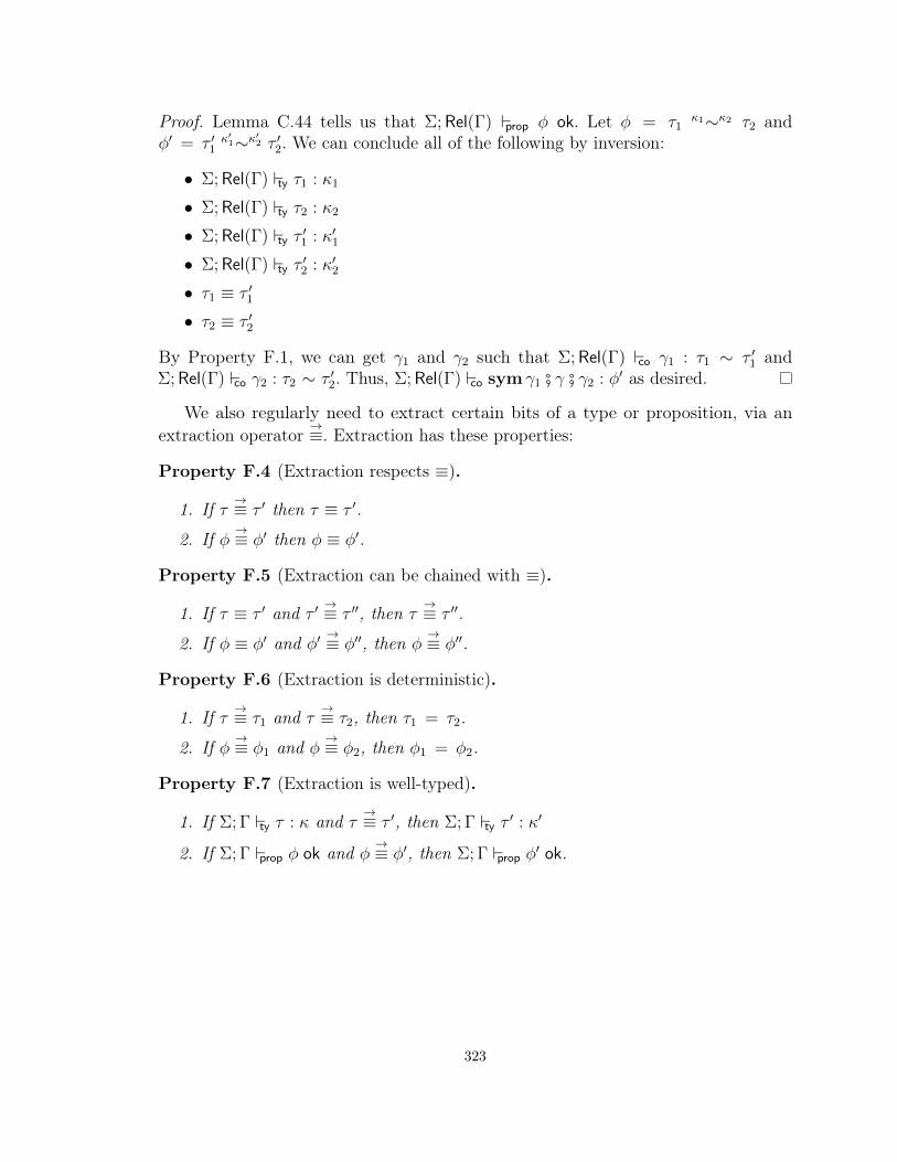
Proof. Lemma C.44 tells us that Σ; Rel(Γ) prop φ ok. Let φ = τ1κ1∼κ2 τ2 and

φ′ = τ ′1κ′1∼κ′2 τ ′2. We can conclude all of the following by inversion:

• Σ; Rel(Γ) ty τ1 : κ1

• Σ; Rel(Γ) ty τ2 : κ2

• Σ; Rel(Γ) ty τ′1 : κ′1

• Σ; Rel(Γ) ty τ′2 : κ′2

• τ1 ≡ τ ′1

• τ2 ≡ τ ′2

By Property F.1, we can get γ1 and γ2 such that Σ; Rel(Γ) co γ1 : τ1 ∼ τ ′1 andΣ; Rel(Γ) co γ2 : τ2 ∼ τ ′2. Thus, Σ; Rel(Γ) co sym γ1 # γ # γ2 : φ′ as desired.

We also regularly need to extract certain bits of a type or proposition, via anextraction operator

→≡. Extraction has these properties:

Property F.4 (Extraction respects ≡).

1. If τ→≡ τ ′ then τ ≡ τ ′.

2. If φ→≡ φ′ then φ ≡ φ′.

Property F.5 (Extraction can be chained with ≡).

1. If τ ≡ τ ′ and τ ′→≡ τ ′′, then τ

→≡ τ ′′.

2. If φ ≡ φ′ and φ′→≡ φ′′, then φ

→≡ φ′′.

Property F.6 (Extraction is deterministic).

1. If τ→≡ τ1 and τ

→≡ τ2, then τ1 = τ2.

2. If φ→≡ φ1 and φ

→≡ φ2, then φ1 = φ2.

Property F.7 (Extraction is well-typed).

1. If Σ; Γ ty τ : κ and τ→≡ τ ′, then Σ; Γ ty τ

′ : κ′

2. If Σ; Γ prop φ ok and φ→≡ φ′, then Σ; Γ prop φ

′ ok.

323

F.3 Lemmas adapted from Appendix CLemma F.8 (Scoping). (as Lemma C.12, but with reference to judgments)

Proof. Similar to the proof for Lemma C.12.

Lemma F.9 (Context regularity). If:

1. Σ; Γ ty τ : κ, OR

2. Σ; Γ co γ : φ, OR

3. Σ; Γ prop φ ok, OR

4. Σ; Γ;σ0 τ0alt alt : κ, OR

5. Σ; Γ vec ψ : ∆, OR

6. Σ ctx Γ ok

Then Σ ctx prefix(Γ) ok and sig Σ ok, where prefix(Γ) is an arbitrary prefix of Γ.Furthermore, both resulting derivations are no larger than the input derivations.

Proof. Straightforward mutual induction.

F.4 Soundness of Pico≡

The following lemma also defines the d·e operation. This deterministic operation isdefined to be the existentially-quantified output of the clauses of the following lemma,as labeled. Note that making sense of d·e requires that the argument be well-formed(that is, the premises of the clause defining the operation must be satisfied). Forexample, dτe is not just an operation over a type τ , but it also requires Σ; Γ ty τ : κas an input.

Lemma F.10 (Pico≡ is sound). The uses of dΓe below depend on Lemma F.9above.

1. If Σ ctx Γ ok, then Σ ctx Γ′ ok where Γ′ ≡ Γ. Let dΓe , Γ′. Furthermore,Rel(dΓe) = dRel(Γ)e and if Γ = Γ0, δ, then dΓe = dΓ0e, δ′.

2. If Σ; Γ ty τ : κ, then Σ; dΓe ty τ′ : κ′ where τ ′ ≡ τ and κ′ ≡ κ. Let dτe , τ ′.

3. If Σ; Γ co γ : φ, then Σ; dΓe co γ′ : φ′ where φ ≡ φ′.

4. If Σ; Γ; σ τalt alt : κ and we have τ ′ and κ′ such that τ ′ ≡ τ and κ′ ≡ κ, thenΣ; dΓe;σ `τ ′alt alt ′ : κ′ where alt ′ ≡ alt . Let dalte , alt ′.

5. If Σ; Γ prop φ ok, then Σ; dΓe prop φ′ ok where φ′ ≡ φ. Let dφe , φ′.

6. If Σ; Γ vec ψ : ∆, then Σ; dΓe vec ψ′: ∆ where ψ

′ ≡ ψ. Let dψe , ψ′.

7. If Σ; Γ s σ −→ τ , Σ; Γ ty σ : κ, and Σ; Γ ty τ : κ, then Σ; dΓe s dσe −→ dτe.

324

Proof. By induction on the typing derivations.

Case DCtx_Nil: Immediate.

Case DCtx_TyVar:

Σ; Rel(Γ) ty κ : τ τ ≡ Typea # Γ Σ ctx Γ ok

Σ ctx Γ, a:ρκ okDCtx_TyVar

We must show Σ ctx dΓe, a:ρκ′ ok for some κ′ ≡ κ. Note that dΓe is well-formed

by the induction hypothesis. The induction hypothesis gives us dκe such thatΣ; Rel(dΓe) ty dκe : τ ′ such that τ ′ ≡ τ . By transitivity of ≡ (Property 7.1), τ ′ ≡Type. We have Σ; Rel(dΓe) ty τ

′ : Type (by Lemma C.43) and Σ; Rel(dΓe) ty

Type : Type (by Lemma C.38 and Lemma C.10). We then use Property F.1 toget γ such that Σ; Rel(dΓe) co γ : τ ′ ∼ Type. Choose κ′ = dκeBγ. We see thatΣ; Rel(dΓe) ty dκeB γ : Type as desired. Property 7.5 tells us that κ ≡ dκeB γ,and so we are done.

Case DCtx_CoVar: By induction.

Case DTy_Var: By induction.

Case DTy_Con: By induction. Note that relating the result type (well-typedin Pico) to the input type (well-typed in Pico≡) by ≡ requires congruence,Property F.2. Congruence is similarly used in many other cases.

Case DTy_AppRel:

Σ; Γ ty τ1 : κ0 κ0→≡ Πa:Relκ1. κ2

Σ; Γ ty τ2 : κ′1 κ1 ≡ κ′1Σ; Γ ty τ1 τ2 : κ2[τ2/a]

DTy_AppRel

The induction hypothesis tells us Σ; dΓe ty dτ1e : κ′0 where κ′0 ≡ κ0, andΣ; dΓe ty dτ2e : κ′′1 where κ′′1 ≡ κ′1. By Property F.5, we get κ′0

→≡ Πa:Relκ1. κ2.By Lemma C.43, we have Σ; Rel(dΓe) ty κ

′0 : Type. Thus by Property F.7, we

get Σ; Rel(dΓe) ty Πa:Relκ1. κ2 : σ. Inversion tells us that σ = Type. We canthus use Property 7.1 and Property F.1 to get γ1 such that Σ; Rel(dΓe) co γ1 :κ′0 ∼ Πa:Relκ1. κ2.

Now, inversion and Lemma C.7 tells us Σ; Rel(dΓe) ty κ1 : Type and LemmaC.43 tells us Σ; Rel(dΓe) ty κ

′′1 : Type. Thus Property 7.1 and Property F.1

give us γ2 such that Σ; Rel(dΓe) co γ2 : κ′′1 ∼ κ1. We now choose dτ1 τ2e ,(dτ1eB γ1) (dτ2eB γ2) and we can see that Σ; dΓe ty dτ1 τ2e : κ2[dτ2eB γ2/a] asdesired. Relating this output kind to the input kind is achieved by Property F.2and Property 7.5.

Case DTy_AppIrrel: Similar to previous case.

325

Case DTy_CApp: Similar to previous cases, but appealing to Lemma F.3.

Case DTy_Pi:

Σ; Γ,Rel(δ) ty κ : τ τ ≡ Type

Σ; Γ ty Πδ. κ : TypeDTy_Pi

The induction hypothesis gives us Σ; dΓ,Rel(δ)e ty dκe : τ ′ where τ ′ ≡ τ . LemmaC.43 tells us Σ; dRel(Γ, δ)e ty τ

′ : Type. We know Σ; dRel(Γ, δ)e ty Type : Typeby Lemma C.38 and Lemma C.10. We can thus use Property F.1 to get γ suchthat Σ; dRel(Γ, δ)e co γ : τ ′ ∼ Type. We can conclude Σ; dΓ,Rel(δ)e ty dκeB γ :Type. By the extra condition in the induction hypothesis for contexts, wecan rewrite this to Σ; dΓe,Rel(δ′) ty dκe B γ : Type, where δ′ ≡ δ. We cannow use Ty_Pi to conclude Σ; dΓe ty Πδ′. (dκeB γ) : Type as desired. Here,dΠδ. κe , Πδ′. (dκeB γ).

Case DTy_Cast:

Σ; Rel(Γ) co γ : κ1 ∼ κ2

Σ; Γ ty τ : κ′1 Σ; Rel(Γ) ty κ2 : σκ1 ≡ κ′1 σ ≡ Type

Σ; Γ ty τ B γ : κ2

DTy_Cast

The induction hypothesis gives us:

• Σ; Rel(dΓe) co γ′ : κ′′1 ∼ κ′′2 with κ′′1 ≡ κ1 and κ′′2 ≡ κ2

• Σ; dΓe ty dτe : κ′′′1 where κ′′′1 ≡ κ′1• Σ; Rel(dΓe) ty dκ2e : σ′ where σ′ ≡ σ

Lemma C.44, Lemma C.43, Property 7.1, and Property F.1 give us γ0 suchthat Σ; Rel(dΓe) co γ0 : κ′′′1 ∼ κ′′1. We can thus use Ty_Cast to get Σ; dΓe ty

dτeB γ0 : κ′′2 as desired.

Case DTy_Case: Along the lines of similar cases. We need Lemma F.8 to establishthat the result type of the scrutinee does not mention the bound telescope ∆.

Other cases: Proceed as above. At this point, we have seen a variety of constructsand how to handle them. The remaining cases are similar, using the propertiesof ≡ and

→≡ to get from a typing derivation in Pico≡ to one in Pico.

326

Bibliography

[1] Thorsten Altenkirch, Conor McBride, and James McKinna. Why dependenttypes matter. 2005. URL http://www.strictlypositive.org/ydtm.ps.gz.

[2] Lennart Augustsson. Compiling pattern matching, pages 368–381. Springer BerlinHeidelberg, Berlin, Heidelberg, 1985. ISBN 978-3-540-39677-2. doi: 10.1007/3-540-15975-4_48. URL http://dx.doi.org/10.1007/3-540-15975-4_48.

[3] Lennart Augustsson. Cayenne—a language with dependent types. In Proc.ACM SIGPLAN International Conference on Functional Programming, ICFP’98, pages 239–250. ACM, 1998.

[4] Christiaan P. R. Baaij. Digital Circuits in Cλash: Functional Specification andType-Directed Synthesis. PhD thesis, University of Twente, 2015.

[5] Patrick Bahr. Composing and decomposing data types: A closed type familiesimplementation of data types à la carte. In Workshop on Generic Programming.ACM, 2014.

[6] Henk Barendregt. Introduction to generalized type systems. J. Funct. Program.,1(2):125–154, 1991.

[7] Bruno Barras and Bruno Bernardo. The implicit calculus of constructions asa programming language with dependent types. In Roberto Amadio, editor,Foundations of Software Science and Computational Structures, FOSSACS 2008,pages 365–379, Budapest, Hungary, 2008. Springer Berlin Heidelberg.

[8] Edwin Brady. Programming and reasoning with algebraic effects and dependenttypes. In International Conference on Functional Programming. ACM, 2013.

[9] Edwin Brady. Idris, a general-purpose dependently typed programming language:Design and implementation. J. Funct. Prog., 23, 2013.

[10] Edwin Brady, Conor McBride, and James McKinna. Inductive families neednot store their indices. In Stefano Berardi, Mario Coppo, and Ferruccio Dami-ani, editors, Types for Proofs and Programs, volume 3085 of Lecture Notes inComputer Science. 2004.

327

[11] Joachim Breitner, Richard A. Eisenberg, Simon Peyton Jones, and StephanieWeirich. Safe zero-cost coercions for Haskell. J. Funct. Program., 26:1–79, 2016.

[12] Luca Cardelli. A polymorphic λ-calculus with Type:Type. Technical report,DEC/Compaq Systems Research Center, 1986. Research report 10.

[13] Chris Casinghino, Vilhelm Sjöberg, and Stephanie Weirich. Step-indexed nor-malization for a language with general recursion. In Proc. 4th Workshop onMathematically Structured Functional Programming, Tallinn, Estonia, pages25–39, 2012.

[14] Chris Casinghino, Vilhelm Sjöberg, and Stephanie Weirich. Combining proofsand programs in a dependently typed language. In Proceedings of the 41stACM SIGPLAN-SIGACT Symposium on Principles of Programming Languages,POPL ’14. ACM, 2014.

[15] Manuel M. T. Chakravarty, Gabriele Keller, and Simon Peyon Jones. Associatedtype synonyms. In International Conference on Functional Programming, ICFP’05. ACM, 2005.

[16] Manuel M. T. Chakravarty, Gabriele Keller, Simon Peyton Jones, and SimonMarlow. Associated types with class. In ACM SIGPLAN-SIGACT Symposiumon Principles of Programming Languages, 2005.

[17] David Raymond Christiansen. A pretty printer that says what it means. Talk,Haskell Implementors Workshop, Vancouver, BC, Canada, 2015. URL https://www.youtube.com/watch?v=m7BBCcIDXSg.

[18] Dominique Clément, Thierry Despeyroux, Gilles Kahn, and Joëlle Despeyroux.A simple applicative language: Mini-ML. In Conference on LISP and FunctionalProgramming, LFP ’86. ACM, 1986.

[19] Thierry Coquand and Gérard Huet. The calculus of constructions. Informationand Computation, 76(2):95 – 120, 1988. ISSN 0890-5401. doi: http://dx.doi.org/10.1016/0890-5401(88)90005-3. URL http://www.sciencedirect.com/science/article/pii/0890540188900053.

[20] Luis Damas. Type Assignment in Programming Languages. PhD thesis, Univer-sity of Edinburgh, 1985.

[21] Nicolaas Govert de Bruijn. Lambda calculus notation with nameless dummies, atool for automatic formula manipulation, with application to the church-rossertheorem. Indagationes Mathematicae (Proceedings), 75(5):381âĂŞ392, 1972.ISSN 1385-7258. doi: 10.1016/1385-7258(72)90034-0. URL http://dx.doi.org/10.1016/1385-7258(72)90034-0.

328

[22] Iavor S. Diatchki. Improving haskell types with SMT. In Proceedings of the2015 ACM SIGPLAN Symposium on Haskell, Haskell ’15. ACM, 2015.

[23] Larry Diehl and Tim Sheard. Generic lookup and update for infinitary inductive-recursive types. In Proceedings of the 1st International Workshop on Type-DrivenDevelopment, TyDe 2016. ACM, 2016.

[24] Joshua Dunfield and Neelakantan R. Krishnaswami. Complete and easy bidirec-tional typechecking for higher-rank polymorphism. In International Conferenceon Functional Programming, ICFP ’13. ACM, 2013.

[25] Richard A. Eisenberg. Dependent types in haskell. Presentation to New YorkCity Haskell Users’ Group, Oct 2014. URL https://github.com/goldfirere/nyc-hug-oct2014.

[26] Richard A. Eisenberg. System FC, as implemented in GHC. Technical ReportMS-CIS-15-09, University of Pennsylvania, 2015. URL https://github.com/ghc/ghc/blob/master/docs/core-spec/core-spec.pdf.

[27] Richard A. Eisenberg. An overabundance of equality: Implementing kind equal-ities into haskell. Technical Report MS-CIS-15-10, University of Pennsylva-nia, 2015. URL http://www.cis.upenn.edu/~eir/papers/2015/equalities/equalities.pdf.

[28] Richard A. Eisenberg and Simon Peyton Jones. Levity polymorphism. Draft,2016. URL http://cs.brynmawr.edu/~rae/papers/2017/levity/levity.pdf.

[29] Richard A. Eisenberg and Jan Stolarek. Promoting functions to type families inHaskell. In ACM SIGPLAN Haskell Symposium, 2014.

[30] Richard A. Eisenberg and Stephanie Weirich. Dependently typed programmingwith singletons. In ACM SIGPLAN Haskell Symposium, 2012.

[31] Richard A. Eisenberg, Dimitrios Vytiniotis, Simon Peyton Jones, and StephanieWeirich. Closed type families with overlapping equations (extended version).Technical Report MS-CIS-13-10, University of Pennsylvania, 2013.

[32] Richard A. Eisenberg, Dimitrios Vytiniotis, Simon Peyton Jones, and StephanieWeirich. Closed type families with overlapping equations. In Principles ofProgramming Languages, POPL ’14. ACM, 2014.

[33] Richard A. Eisenberg, Stephanie Weirich, and Hamidhasan Ahmed. Visibletype application. In European Symposium on Programming (ESOP), LNCS.Springer-Verlag, 2016.

329

[34] Richard A. Eisenberg, Stephanie Weirich, and Hamidhasan Ahmed. Visible typeapplication (extended version). 2016. URL http://www.cis.upenn.edu/~eir/papers/2016/type-app/visible-type-app-extended.pdf.

[35] Jeff Epstein, Andrew P. Black, and Simon Peyton Jones. Towards haskell in thecloud. In Haskell Symposium. ACM, 2011.

[36] Jean-Yves Girard. Interprétation fonctionnelle et élimination des coupures del’arithmétique d’ordre supérieur. PhD thesis, Université Paris 7, 1972.

[37] Adam Gundry. Type Inference, Haskell and Dependent Types. PhD thesis,University of Strathclyde, 2013.

[38] Adam Gundry. A typechecker plugin for units of measure: Domain-specificconstraint solving in GHC Haskell. In Proceedings of the 2015 ACM SIGPLANSymposium on Haskell, Haskell ’15. ACM, 2015.

[39] Cordelia V. Hall, Kevin Hammond, Simon L. Peyton Jones, and Philip L. Wadler.Type classes in haskell. ACM Trans. Program. Lang. Syst., 18(2), March 1996.

[40] Bastiaan Heeren, Daan Leijen, and Arjan van IJzendoorn. Helium, for learninghaskell. In Workshop on Haskell. ACM, 2003.

[41] Fritz Henglein. Type inference with polymorphic recursion. ACM Trans. Program.Lang. Syst., 15(2):253–289, April 1993. ISSN 0164-0925. doi: 10.1145/169701.169692. URL http://doi.acm.org/10.1145/169701.169692.

[42] Jason J. Hickey. Formal objects in type theory using very dependent types.In Foundations of Object Oriented Languages (FOOL ’96), 1996. URL http://www.cis.upenn.edu/~bcpierce/FOOL/FOOL3.html.

[43] J. Roger Hindley. The principal type-scheme of an object in combinatory logic.Transactions of the American Mathematical Society, 146, 1969.

[44] Martin Hofmann and Thomas Streicher. The groupoid interpretation of typetheory. In Giovanni Sambin and Jan M. Smith, editors, Twenty-Five Years ofConstructive Type Theory, Oxford Logic Guides, Venice, Italy, 1995. OxfordUniversity Press.

[45] Paul Hudak, John Hughes, Simon Peyton Jones, and Philip Wadler. A historyof haskell: Being lazy with class. In Conference on History of ProgrammingLanguages, 2007.

[46] John Hughes. Generalising monads to arrows. Sci. Comput. Program., 37(1-3),May 2000.

330

[47] Chung-Kil Hur. Agda with excluded middle is inconsistent. Email to Agdamailing list, January 2010. URL https://lists.chalmers.se/pipermail/agda/2010/001526.html.

[48] Antonius J. C. Hurkens. A simplification of Girard’s paradox, pages 266–278.Springer Berlin Heidelberg, Berlin, Heidelberg, 1995. ISBN 978-3-540-49178-1.doi: 10.1007/BFb0014058. URL http://dx.doi.org/10.1007/BFb0014058.

[49] Mark P. Jones. Type classes with functional dependencies. In European Sympo-sium on Programming, 2000.

[50] Stefan Kahrs and Connor Smith. Non-Omega-Overlapping TRSs are UN. InDelia Kesner and Brigitte Pientka, editors, 1st International Conference onFormal Structures for Computation and Deduction (FSCD 2016), volume 52of Leibniz International Proceedings in Informatics (LIPIcs), pages 22:1–22:17,Dagstuhl, Germany, 2016. Schloss Dagstuhl–Leibniz-Zentrum fuer Informatik.ISBN 978-3-95977-010-1. doi: http://dx.doi.org/10.4230/LIPIcs.FSCD.2016.22.URL http://drops.dagstuhl.de/opus/volltexte/2016/5996.

[51] Georgios Karachalias, Tom Schrijvers, Dimitrios Vytiniotis, and Simon Pey-ton Jones. GADTs meet their match. In International Conference on FunctionalProgramming, ICFP ’15. ACM, 2015.

[52] Oleg Kiselyov, Ralf Lämmel, and Keean Schupke. Strongly typed heterogeneouscollections. In Proc. 2004 ACM SIGPLAN Workshop on Haskell, Haskell ’04,pages 96–107. ACM, 2004.

[53] Ralf Lämmel and Simon Peyton Jones. Scrap your boilerplate: A practicaldesign pattern for generic programming. In Workshop on Types in LanguagesDesign and Implementation. ACM, 2003.

[54] K. Rustan M. Leino. Dafny: An automatic program verifier for functionalcorrectness. In Edmund M. Clarke and Andrei Voronkov, editors, Logic forProgramming, Artificial Intelligence, and Reasoning, LPAR’16, pages 348–370.Springer Berlin Heidelberg, 2010.

[55] Sheng Liang, Paul Hudak, and Mark Jones. Monad transformers and modularinterpreters. In Proceedings of the 22Nd ACM SIGPLAN-SIGACT Symposiumon Principles of Programming Languages, POPL ’95. ACM, 1995.

[56] Sam Lindley and Conor McBride. Hasochism: the pleasure and pain of depen-dently typed Haskell programming. In ACM SIGPLAN Haskell Symposium,2013.

[57] Zhaohui Luo. An Extended Calculus of Constructions. PhD thesis, University ofEdinburgh, 1990.

331

[58] Conor McBride. Dependently Typed Functional Programs and their Proofs. PhDthesis, University of Edinburgh, 1999. URL http://strictlypositive.org/thesis.pdf.

[59] Conor McBride. Faking it: Simulating dependent types in Haskell. J. Funct.Program., 12(5):375–392, July 2002.

[60] Conor McBride. The Strathclyde Haskell Enhancement. https://personal.cis.strath.ac.uk/conor.mcbride/pub/she/, 2011.

[61] Conor Thomas McBride. How to keep your neighbours in order. In Proceedings ofthe 19th ACM SIGPLAN International Conference on Functional Programming,ICFP ’14. ACM, 2014.

[62] Lambert Meertens. Incremental polymorphic type checking in B. In Proceedingsof the 10th ACM SIGACT-SIGPLAN Symposium on Principles of ProgrammingLanguages, POPL ’83. ACM, 1983.

[63] Robin Milner. A Theory of Type Polymorphism in Programming. Journal ofComputer and System Sciences, 17, 1978.

[64] Alexandre Miquel. The implicit calculus of constructions: Extending pure typesystems with an intersection type binder and subtyping. In Samson Abramsky,editor, Typed Lambda Calculi and Applications, volume 2044 of Lecture Notes inComputer Science, pages 344–359. Springer Berlin Heidelberg, 2001.

[65] Nathan Mishra-Linger and Tim Sheard. Erasure and polymorphism in puretype systems. In Foundations of Software Science and Computational Structures(FoSSaCS). Springer, 2008.

[66] J. Garrett Morris and Mark P. Jones. Instance chains: type class programmingwithout overlapping instances. In ACM SIGPLAN International Conference onFunctional Programming, 2010.

[67] Alan Mycroft. Polymorphic type schemes and recursive definitions. Springer,Berlin, Heidelberg, 1984.

[68] Ulf Norell. Towards a practical programming language based on dependent typetheory. PhD thesis, Department of Computer Science and Engineering, ChalmersUniversity of Technology, SE-412 96 Göteborg, Sweden, September 2007.

[69] Nicolas Oury and Wouter Swierstra. The power of Pi. In Proc. 13th ACMSIGPLAN international conference on Functional programming, ICFP ’08, pages39–50. ACM, 2008.

[70] Conrad Parker. Type-level instant insanity. The Monad.Reader, (8), 2007.

332

[71] Simon Peyton Jones, editor. Haskell 98 Language and Libraries: The RevisedReport. Cambridge University Press, 2003.

[72] Simon Peyton Jones and Mark Shields. Lexically-scoped type variables. Draft,2004. URL http://research.microsoft.com/en-us/um/people/simonpj/papers/scoped-tyvars/.

[73] Simon Peyton Jones, Andrew Tolmach, and Tony Hoare. Playing by the rules:rewriting as a practical optimisation technique in GHC. In Haskell Workshop,pages 203–233, 2001.

[74] Simon Peyton Jones, Dimitrios Vytiniotis, Stephanie Weirich, and Mark Shields.Practical type inference for arbitrary-rank types. Journal of Functional Pro-gramming, 17(1), January 2007.

[75] Simon Peyton Jones, Stephanie Weirich, Richard A. Eisenberg, and DimitriosVytiniotis. A reflection on types. In A list of successes that can change the world,LNCS. Springer, 2016. A festschrift in honor of Phil Wadler.

[76] Matthew Pickering, Gergő Érdi, Simon Peyton Jones, and Richard A. Eisenberg.Pattern synonyms. In ACM SIGPLAN Haskell Symposium. ACM, 2016.

[77] Benjamin C. Pierce. Types and Programming Languages. MIT Press, Cambridge,MA, 2002.

[78] Benjamin C. Pierce and David N. Turner. Local type inference. ACM Trans.Program. Lang. Syst., 22(1), January 2000.

[79] François Pottier and Didier Rémy. Advanced Topics in Types and ProgrammingLanguages, chapter The Essence of ML Type Inference, pages 387–489. TheMIT Press, 2005.

[80] Bertrand Russell. Mathematical llogic as based on a theory of types. Amer. J.Math., 30:222–262, 1908.

[81] Alejandro Serrano Mena. Beginning Haskell: A Project-Based Approach. Apress,2013.

[82] Peter Sewell, Francesco Zappa Nardelli, Scott Owens, Gilles Peskine, ThomasRidge, Susmit Sarkar, and Rok Strniša. Ott: Effective tool support for theworking semanticist. Journal of Functional Programming, 20(1), January 2010.

[83] Tim Sheard and Simon Peyton Jones. Template meta-programming for Haskell.In Proc. 2002 ACM SIGPLAN workshop on Haskell, Haskell ’02, pages 1–16.ACM, 2002.

333

[84] Vincent Simonet and François Pottier. A constraint-based approach to guardedalgebraic data types. ACM Trans. Program. Lang. Syst., 29(1), January 2007.

[85] Vilhelm Sjöberg and Stephanie Weirich. Programming up to congruence. In Pro-ceedings of the 42Nd Annual ACM SIGPLAN-SIGACT Symposium on Principlesof Programming Languages, POPL ’15. ACM, 2015.

[86] Jan Stolarek, Simon Peyon Jones, and Richard A. Eisenberg. Injective typefamilies for Haskell. In Haskell Symposium, Haskell ’15. ACM, 2015.

[87] Martin Sulzmann, Manuel M. T. Chakravarty, Simon Peyton Jones, and KevinDonnelly. System F with type equality coercions. In Types in languages designand implementation, TLDI ’07. ACM, 2007.

[88] Martin Sulzmann, Gregory J. Duck, Simon Peyton-Jones, and Peter J. Stuckey.Understanding functional dependencies via constraint handling rules. J. Funct.Program., 17(1), January 2007.

[89] Nikhil Swamy, Cătălin Hriţcu, Chantal Keller, Aseem Rastogi, Antoine Delignat-Lavaud, Simon Forest, Karthikeyan Bhargavan, Cédric Fournet, Pierre-YvesStrub, Markulf Kohlweiss, Jean-Karim Zinzindohoue, and Santiago Zanella-Béguelin. Dependent types and multi-monadic effects in F?. In Proceedingsof the 43rd Annual ACM SIGPLAN-SIGACT Symposium on Principles ofProgramming Languages, POPL ’16. ACM, 2016.

[90] Matúš Tejiščák and Edwin Brady. Practical erasure in dependently typedlanguages. Draft, 2015. URL http://eb.host.cs.st-andrews.ac.uk/drafts/dtp-erasure-draft.pdf.

[91] The Univalent Foundations Program. Homotopy Type Theory: Univalent Foun-dations of Mathematics. https://homotopytypetheory.org/book, Institutefor Advanced Study, 2013.

[92] Floris van Doorn, Herman Geuvers, and Freek Wiedijk. Explicit convertibilityproofs in pure type systems. In Proceedings of the Eighth ACM SIGPLANInternational Workshop on Logical Frameworks and Meta-languages: Theory andPractice, LFMTP ’13, pages 25–36, New York, NY, USA, 2013. ACM. ISBN978-1-4503-2382-6. doi: 10.1145/2503887.2503890. URL http://doi.acm.org/10.1145/2503887.2503890.

[93] Niki Vazou, Eric L. Seidel, and Ranjit Jhala. LiquidHaskell: Experience withrefinement types in the real world. In Proceedings of the 2014 ACM SIGPLANSymposium on Haskell, Haskell ’14. ACM, 2014.

[94] Niki Vazou, Eric L. Seidel, Ranjit Jhala, Dimitrios Vytiniotis, and Simon Pey-ton Jones. Refinement types for Haskell. In International Conference onFunctional Programming, ICFP ’14. ACM, 2014.

334

[95] Niki Vazou, Alexander Bakst, and Ranjit Jhala. Bounded refinement types. InProceedings of the 20th ACM SIGPLAN International Conference on FunctionalProgramming, ICFP 2015. ACM, 2015.

[96] Dimitrios Vytiniotis and Simon Peyton Jones. Evidence Normalization in Sys-tem FC. In Femke van Raamsdonk, editor, 24th International Conferenceon Rewriting Techniques and Applications (RTA 2013), volume 21 of Leib-niz International Proceedings in Informatics (LIPIcs), pages 20–38, Dagstuhl,Germany, 2013. Schloss Dagstuhl–Leibniz-Zentrum fuer Informatik. ISBN978-3-939897-53-8. doi: http://dx.doi.org/10.4230/LIPIcs.RTA.2013.20. URLhttp://drops.dagstuhl.de/opus/volltexte/2013/4050.

[97] Dimitrios Vytiniotis, Stephanie Weirich, and Simon Peyton Jones. Boxy types:Inference for higher-rank types and impredicativity. In International Conferenceon Functional Programming, ICFP ’06. ACM, 2006.

[98] Dimitrios Vytiniotis, Simon Peyton Jones, and Tom Schrijvers. Let should notbe generalized. In Types in Language Design and Implementation, TLDI ’10.ACM, 2010.

[99] Dimitrios Vytiniotis, Simon Peyton Jones, Tom Schrijvers, and Martin Sulzmann.OutsideIn(X): Modular type inference with local assumptions. Journal ofFunctional Programming, 21(4-5), September 2011.

[100] Dimitrios Vytiniotis, Simon Peyton Jones, and José Pedro Magalhães. Equalityproofs and deferred type errors: A compiler pearl. In International Conferenceon Functional Programming, ICFP ’12. ACM, 2012.

[101] Philip Wadler. Compiling pattern matching. In Simon Peyton Jones, editor,The Implementation of Functional Programming Languages. Prentice-Hall, 1987.

[102] Philip Wadler and Stephen Blott. How to make ad-hoc polymorphism lessad-hoc. In POPL, pages 60–76. ACM, 1989.

[103] Geoffrey Washburn and Stephanie Weirich. Boxes Go Bananas: Encodinghigher-order abstract syntax with parametric polymorphism. In InternationalConference on Functional Programming. ACM, 2003.

[104] Stephanie Weirich. Paradoxical typecase. Presentation to WG2.8., November2012. URL http://www.cis.upenn.edu/~sweirich/talks/wg28-paradoxes.pdf.

[105] Stephanie Weirich, Justin Hsu, and Richard A. Eisenberg. System FC withexplicit kind equality. In International Conference on Functional Programming,ICFP ’13. ACM, 2013.

335

[106] Stephanie Weirich, Justin Hsu, and Richard A. Eisenberg. System FC with ex-plicit kind equality (extended version). Technical report, University of Pennsylva-nia, 2013. URL http://www.cis.upenn.edu/~sweirich/nokinds-extended.pdf.

[107] Brent A. Yorgey, Stephanie Weirich, Julien Cretin, Simon Peyton Jones, Dim-itrios Vytiniotis, and José Pedro Magalhães. Giving Haskell a promotion. InTypes in Language Design and Implementation, TLDI ’12. ACM, 2012.

336