depreciation manipulation and its impact on firms’ returns
TRANSCRIPT

A Work Project, presented as part of the requirements for the Award of a Masters
Degree in Finance from the Faculdade de Economia da Universidade Nova de Lisboa
Depreciation manipulation and its impact on firms’ returns
Kristina Vadeikaite
Mst16000210
A Project carried in Finance, with the supervision of
Professor Ana Marques
January, 2010

1
Abstract
Earnings management is typically achieved via discretionary accruals (such as
depreciation). Dechow et al. (1996), Archibald (1972), and Peasnell et al. (2000) present
results on the market reaction to depreciation manipulation that are inconsistent. They find
either no reaction or a negative one. This study aims at settling this contradiction by using
several different methods, in order to identify a possible manipulation, with a sample of
S&P500 firms.
Data suggests that firms are manipulating depreciation. Furthermore, an analysis of useful
life of assets reveals that firms have been increasing it since the dot com bubble burst and
that its value is larger in profitable firms. However, results of our event studies reveal that
the market is not reacting to deprecation manipulation. Thus, it seems possible for firms to
fool the markets via this specific manipulation.
Keywords Depreciation manipulation; Earnings management; Market reaction
2
1. Introduction
Depreciation is one of the accounting activities that has a sizable impact on companies’
profits. There is some flexibility for calculating the value of depreciation, which in turn
allows firms to window-dress their accounts to a certain extent. Depreciation manipulation
is a tool of earnings management and, according to Bartov (1993), can be classified as an
act of earnings-smoothing. Brenton and Stolowy (2004) state that the ―additional‖ fund
(result of the manipulation of depreciation) can be saved over the good times and used over
the bad ones, in this way smoothing the normal fluctuation of earnings.
Manipulation of depreciation can be achieved in two ways: via switching depreciation
method or changing estimation of assets useful life. The key reasons behind these changes
are an aspiration to increase profits and a need to be comparable with the industry
accounting standards (Healy and Wahlen, 1999). Comiskey (1971) indicates that a change
from accelerated to straight line depreciation accounting method increases the reported
earnings per share in all the companies included in her study of the steel market. Dechow et
al. (1996) indicate that once earnings manipulation becomes known to the public, the price
of the share drops accordingly to the amount that is perceived to be overstated. Archibald
(1972) does not find abnormal performance of the stock during the announcement of the
change of depreciation method. However, Peasnell et al. (2000), state that earnings
management through depreciation manipulation is ―a somewhat transparent‖, and thus it
does make an impact to the market price of the firm
Plummer and Mets (2001) comment that ―although prior researches suggest that firms
manage earnings to achieve certain reporting objectives, the literature provides limited
evidence on which specific components or accruals are used for earnings management‖.
3
This study aims to enrich existing earnings management literature by studying financial
markets’ reactions to the manipulation of depreciation. In order to identify the possible
manipulation, four different depreciation manipulation proxies have been used. The first
two estimate the value of abnormal depreciation (following the methodologies of
Marquardt and Wiedman’s (2004) and Jennings and Marques (2006) (unpublished)), the
third one is depreciation index (Beneish’s (1997) method) and the final one is useful life of
assets (Jennings and Marques (2006) (unpublished)). The sample consists of firms from the
Standard & Poor’s 500 Index (S&P500) and the data covers a period of 9 years (from 1999
to 2007).
The study yields three important results. First, by using four different methodologies it is
found that firms manipulate depreciation to a certain extent. Second, useful life of asset
over the sample has a tendency to increase since dot com burst bubble and is superior in
profitable companies, which might imply that firms manipulate depreciation for earnings
management. Third, four regressions (two with variable of interest abnormal depreciation,
one with depreciation index and one with useful life of assets) yield the same result, that is
market does not react to depreciation manipulation.
This paper contributes to the literature on earnings management which, according to Bartov
(1993) and Hillier and McCrae (1998) is quite unexplored. Moreover, the study resolves the
dispute in the existing literature on depreciation manipulation. The study uses formula
created by Jennings and Marques (2006), which has never been published, thus the paper
helps to get the work of authors public. The results obtained by employing four different
methodologies give a new perspective on depreciation manipulation for a ―real market‖, to
be more precise firms can mislead market via the calculation of the depreciation expense,

4
as market does not react to this manipulation. Finally, the paper creates new questions and
areas for exploration in finance research literature.
The remainder of the paper is organized as follows. The next section reviews pertinent
literature and develops the research questions. Section three explains how the final sample
was obtained. Section four outlines the methodology used in this study. Section five reports
the descriptive statistics and reports the results. The last section concludes the paper and
suggests some lines for future research.
2. Literature review and research questions
2.1 Earnings manipulation and management
In finance, manipulation can be defined as an act where false signal or information is being
sent in order to make investors purchase or vend specific securities, to make a gain out of
this operation (Ogut et al., 2009). It can be classified into three categories, as it can be
action-based, trade-based or information-based manipulation (Allan and Gale, 1992).
Financial information manipulation is also called accounting manipulation and, according
to Beneish (2001), it is vaguely different from earnings management. As a result, the two
terms are sometimes used interchangeably. Earnings manipulation can be defined as
―intentional misstatements or omissions of amounts and disclosures in financial statements
to deceive users‖ (Arens and Loebbecke, 2000). On the other hand, earnings management
has been defined by Healy and Wahlen (1999), which state that ―earnings management is
an action where managers apply judgment in constructing transaction or in financial
reporting to modify financial reports, in order to mislead shareholder about the firm’s

5
financial performance or make an impact on contractual outcomes that depend on this
information‖.
According to Ayres (1994) there are three ways of managing earnings. The first is accrual
management, which can be explained as a desire to modify earnings by varying items such
as useful lives, probability to recover debts and other. The second way is to alter the timing
of the introduction of obligatory accounting policies. The final way is to change from one
accounting method to another.
2.2 Reasons and consequences of earnings management
Healy and Wahlen (1999) find three main reasons for earning management: capital market
motivations, regulation and contract motivation. Some examples of capital market
motivation are found in Dechow et al.’s (1996) research, which point out that significant
stimulus for earnings manipulation is an aspiration to attract external financing at low cost
and to avoid debt covenant restrictions. Moreover, Stubben (2006) reveals that accruals
management is being used to meet firms’ earnings and sales forecasts. Regulation motives
are found by Altamuro et al. (2005), which indicate that companies manipulate revenue
recognition due to the desire to meet industry benchmarks. Finally, contractual motivation
can be portrayed by Bartov (1993) research, where the author introduces earnings-
smoothing (when earnings manipulating is being used to reduce the fluctuation from the
company’s normal state) and debt-equity hypothesis (positive correlation exists between
debt to equity ratio and earnings manipulation).
6
Earnings management has several consequences on company’s results and its appearance to
the stakeholders. Barton and Simko (2002) find that authors reveal that ―the penalty
imposed by the market per penny of earnings per share (EPS) missed is more severe for
firms missing by a penny than by a larger amount―. Dechow et al. (1996) indicate that once
earnings manipulation becomes known to the public, the price of the share drops
accordingly to the amount that is perceived to be overstated. Consequently, the cost of
capital for these companies increases. Beneish (1997) finds that companies that have
violated GAAP, in order to favorably improve the financial reports, experience abnormal
negative returns for the following two years.
2.3 Depreciation manipulation
One way to manage earnings is to smooth them by manipulating depreciation. As there is
some flexibility for calculation of the depreciation amount, firms may window-dress their
accounts to a certain extent (Brenton and Stolowy, 2004). Beck (2003) quotes Wexler
(economist at Merrill Lynch, 2001), which states that depreciation manipulation accounted
for 25% of the improvements in second-quarter profits (S&P500 firms). Hiller and Mccrae
(1998) study the earnings smoothing potential of systematic depreciation and find that
manipulation can be achieved in two ways: (i) via switching depreciation method and (ii)
changing estimation of assets’ useful life.
Switching depreciation methods: Myers (1967) was the first to analyze this topic. The
author finds that the switch of depreciation method by companies in 1965 and 1966 had a
positive impact on earnings per share. The author also notes that depreciation manipulation
can be done only once and that the impact of this kind of earnings management is
7
restricted. For instance, the switch of depreciation method allows firm to build up an
―earnings bank‖, which will be used upcoming year and the need to have another one will
require to change accounting procedures once more1. Comiskey (1971) indicates that a
change from accelerated to straight line depreciation accounting method increases the
reported earnings per share in all the companies included in her study of the steel market.
Archibald (1972) does not find abnormal performance of the stock during the
announcement of the change of depreciation method. Finally, Jackson et al. (2008) find
that the number of firms using accelerated depreciation method for all or some of their
depreciable assets have dropped from roughly 31 percent in 1988 to around 14 percent in
2006. Results indicate that the choice of depreciation method makes an impact on firm’s
management decisions regarding limited capital resource.
Changing the estimation of useful life of assets’: Bartov (1993) reveals that income from
the sale of assets in the companies that experience low income are higher than in the ones
who are having high incomes, which suggests the conclusion of manipulation of timing of
the assets. More recent research by Gunny (2005) indicates that manipulation of timing of
asset sale (in a sense of earnings management) has a negative economic impact on the
operating results of the following period (earnings and cash flow). Herrmann et al. (2003)
reveal that ―in case firms report current operating income is below (above) management's
forecasted number, firms tend to increase (decrease) earnings through the sale of fixed
assets‖ (this research was conducted on Japanese firms).
1According to Myers (1967) earnings bank refers to additional money that stays in a firm when depreciation method is changed.

8
2.4 Research questions
Plummer and Mets (2001) comment that although prior research suggests that ―firms
manage earnings to achieve certain reporting objectives, the literature provides limited
evidence on which specific components or accruals are used for earnings management‖.
Hillier and McCrae (1998) state that although there were numerous studies made on
earnings smoothening, ―only a few of those has concentrated on depreciation‖. Bartov
(1993) also indicates that the potential of depreciation to smoothen earnings
and ability to manipulate depreciation method is quite unexplored. This paper aims at
filling the gap that is present in the earnings management literature with regard to
depreciation manipulation. Specifically, two research questions will be addressed. The first
is whether firms currently manage earnings via depreciation expenses. If the answer to the
first research question is positive the second research question is whether the market reacts
to this manipulation. Finding a negative market reaction for manipulation would indicate
that capital markets can see through manager’s manipulation of this value. On the other
hand, finding no market reaction suggests that firms can fool the market via the calculation
of the depreciation expense.
3. Sample
The sample selection process begins with all firms included in the S&P500. According to
Perry et al. (2001), this index is relevant due to its economic significance, more precisely
size of the firms. Laudicina (2005) state that results reported by the S&P 500 firms are
more applicable to the research, as it is most generally referenced U.S. equity standard.
Research is conducted using yearly financial statements. Ogut et al. (2009) state that even

9
though manipulation of accounting methods can occur in the middle of the year, it is
important to study year-end financial statements, as they are accessible for public use and
are employed by investors and analysts.
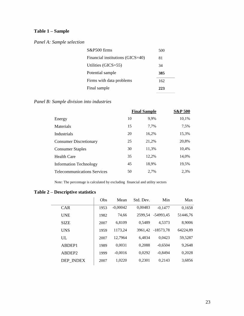
The calculation of the firms included in the final sample is described in Table 1. Firms
belonging to financial and utilities industries were excluded due to their specific regulation.
This is done by using the Global Industry Classification Standards (GICS), which
according to Bhojraj et al. (2003), are significantly better in various settings of capital
markets research than other industry classification schemes. This yields a potential sample
of 385 firms. Due to time constraints, we randomly select 223 firms. The sample period
covers a period of 9 years (from 1998 to 2007).
Data is collected from two sources. First, the information needed for the calculation of
abnormal depreciation and useful life of assets is retrieved from Compustat quarterly
database. Second, market reaction information is collected from CRSP.
4. Methodology
In this study we use four different proxies for identification of depreciation manipulation.
The first two are measures of abnormal depreciation. The third is a measure of depreciation
index. The fourth proxy is a measure of manipulation of the useful life of assets. Each one
of these proxies is then used in an event study, in order to assess if the market reacts to
firms that manipulate depreciation when the earnings announcements are made.

10
4.1. Measures of abnormal depreciation, depreciation index and manipulation of
useful life
The first abnormal depreciation variable (ABDEP1) is calculated following Marquardt and
Wiedman’s (2004) method. It is based on the calculation of the expected value of
depreciation, which is assumed to remain a constant in proportion with gross property,
plant, and equipment and its subtraction from the ―real‖ value of depreciation.
, , 1 , , 1 , 1ABDEP1 * & / & /j t j t j t j t j tDEP DEP GrossPP E GrossPP E TA
Net depreciation (Q2), coded as ―Depreciation Net Qtly‖ in Compustat.
Gross PP&E (Q), coded as ―PP&E-Total Gross Qtly‖ in Compustat.
Total Assets (Q), coded as ―Total Assets Qtly‖ in Compustat.
The second abnormal depreciation variable (ABDEP2) and useful life of asset (UL) is
calculated by using formula created by Jennings and Marques (2006)3. Authors, after the
revision of existing literature, look at a case study of ―Waste Management, Inc.‖, which
mentions three items to be compared at an industry level: percent of Net PP&E in Assets
(capital intensity), useful life, and a ration of depreciation/revenues. Thus, authors suggest
calculating useful life of asset. The analysis of this item should portray the willingness to
manipulate depreciation.
onDepreciati
EPMeanGrossPUL
&
2 Q - quarterly data 3 Jennings and Marques was working on the topic ―The manipulation depreciation‖, though the paper has not been published. The paper
aimed at ―assesing if or not there has been recent and widespread manipulation of earningsm via changes in depreciation plocies‖. Furthermore, second step was to investigate possible consequences of manipulation. I would like to thank for Prof. Ana Marques
(Universidade Nova de Lisboa) and Prof. Ross Jennings (University of Texas at Austin) for allowing using thier unpublished formulas
and findings.

11
Gross depreciation (Q), coded as ―Depreciation Gross Qtly‖ in Compustat.
Gross PP&E (Q), coded as ―PP&E-Total Gross Qtly‖ in Compustat.
The useful life of asset is an important item for the calculation of unexpected depreciation.
&ABDEP2
MeanGrossPP EDepreciation
lagUL
Gross depreciation (Q), coded as ―Depreciation Gross Qtly‖ in Compustat.
Gross PP&E (Q), coded as ―PP&E-Total Gross Qtly‖ in Compustat.
It is important to emphasize that the calculation might be biased due the fact that
Compustat database yield depreciation and amortization as one item named depreciation
and there is none specific item for land.
The third depreciation variable (DEP_INDEX) is calculated by using Beneish’s (1997)
methodology. The author indicates that a depreciation index greater than one is an indicator
of the slow down of the rate by which assets have been depreciated. This can occur due to
two reasons: firm has switched its depreciation method in order to increase earnings or
estimation of asset’s useful life has been raised.
1 1 1/ ( & )DEP _ INDEX
/ ( & )
t t t
t t t
Depreciation Depreciation PP E
Depreciation Depreciation PP E
Gross depreciation (Q), coded as ―Depreciation Gross Qtly‖ in Compustat.
Gross PP&E (Q), coded as ―PP&E-Total Gross Qtly‖ in Compustat.
These results can be sorted by applying Zatta (2005) criteria. This is needed to be done as
―indexes are not foolproof and have frequently produced erroneous results‖ (Harrington,

12
2005). According to Zatta (2005), the depreciation index needs to be interpreted by looking
at it in the multiple period samples. Moreover, the author states ―if the rate of depreciation
falls over two periods, it raises the possibility that the company has boosted its estimates of
assets’ useful lives or adopted a new depreciation method that increases income‖. This
method yielded 23 companies in the sample, which probably manipulated depreciation. For
these companies an indicator variable is created, in which manipulators are coded as 1 and
non-manipulators as 0.
4.2. Reaction to abnormal depreciation and manipulation of useful life
The next part of this study tests market reactions to the abnormal depreciation and the
manipulation of the useful life of assets. Equations 1, 2 and 3 correspond to the three
different proxies for abnormal depreciation discussed above. Equation 4 analyzes the
reaction to the manipulation of useful life. The models are as follows:
CAR = 0
variables of interest: + 1 ABDEP1
other variables: + 2 UNE + 3UNS + 4 SIZE (1)
CAR = 0
variables of interest: + 1 ABDEP2
other variables: + 2 UNE + 3UNS + 4 SIZE (2)
CAR = 0
variables of interest: + 1 DEP_INDEX
other variables: + 2 UNE + 3UNS + 4 SIZE+ 5DM (3)
CAR = 0
variables of interest: + 1 UL
other variables: + 2 UNE + 3UNS + 4 SIZE (4)

13
In order to measure market reaction, an event study is conducted, with its 3-day window
centred at the date of the earnings announcement. The study is made by using the 4th
quarter earnings’ announcement day, as it contains the yearly performance of the company.
Normal return in this study refers to the firm-specific daily return, while the expected return
is calculated using a value-weighted index.
The control variables used in regressions were unexpected earnings (UNE), unexpected
sales (UNS), and size (SIZE). According to Hsu (2002), unexpected earnings occur when
company’s reported earnings deviate from analysts’ forecasts and are considered to be a
useful tool in predicting abnormal returns. In this study, unexpected earnings are calculated
as a real value minus value of the same quarter last year. Moreover, unexpected sales are
calculated in the same manner. According to Kothari (2001), the size of a company is
related to the abnormal returns during earnings announcement days. This variable is
calculated as natural logarithm of total assets.
5. Findings
5.1. Descriptive statistics
Descriptive statistics of all variables used in the four regressions, before scaling the data
and excluding outliers are presented in table 3. As we can see from the table, dependent
variable CAR is varying substantially. According to Seiler (2000), this variability could
have been caused by the type of methodology used to perform the event study. Extreme
data points are found in unexpected earning and unexpected sales variables as well. These
could be explained by the nature of S&P500 as it is composed of companies of different
size, belonging to diverse sectors. The descriptive statistics of variables of interest indicates

14
outliers that could be further investigated for earning manipulation. For example,
DEP_INDEX has a maximum value of 3,68 (and more than one suggest earnings
management).
According to Evans (1997), outliers’ identification is significant in regression analysis as
outliers can impact model in such way that it will make the conclusions of study biased. In
order to eliminate this impact, 2% of extreme data points are removed (1% from each side).
As expected, this procedure increased adjusted R-squared of the regression lines. The first
regression, for example, had a adjusted R-squared of 0,4% before procedure and 5,47%
after it. In addition to that, scaling is made by dividing variables by market value, as this
procedure allows normalizing data.
Table 3 shows the correlation between variables. The table depict that variables have a
weak (coefficient from -0,2 to 0,2) relationship (by Pearson and Spearman correlation)4,
where the strongest one are seen between CAR and unexpected sales and the two of the
proxies for abnormal depreciation, ABDEP1 and ABDEP2, which are also strongly
correlated (0,684). Moreover, this relationship is statistically significant (p-value of 0.000).
All of the regressions have positive significant correlation between CAR and unexpected
sales, which suggests that market reacts positively to unexpected sales (as expected in line
with Hsu, 2002). On the other hand, the table depict that there is a low positive correlation
between CAR and ABDEP1, and ABDEP2 (respectively 0,018 and 0,011), suggesting that
when abnormal depreciation is increasing CAR is increasing as well, and low negative
correlation between CAR and DEP_INDEX, and UL (respectively -0,03 and -0,014),
suggesting that when abnormal depreciation or useful life of asset is increasing CAR is
4 Spearman correlation indicates relationship between X and Y, when they are related by any monotonic fuction, while Pearson
correlation is a result of a linear fuction between X and Y.
15
decreasing. In addition, table 3 shows that significance correlation is found between UL
and SIZE (0,030), UNE and SIZE (0,006) ABDEP1 and UNS (0,005), UNS and SIZE
(0,041), ABDEP2 and SIZE (0,013), and UNE and SIZE (0,001).
Table 4, panel A presents analysis of useful life of assets for a timeframe from 1999 to
2007. This suggests that, on average, until the ―dot com bubble burst‖ the useful life of the
assets in the sample companies was decreasing and after this event it has a tendency to
increase. This implies smaller depreciation expenses and larger net income (2001-
onwords), which is an important figure for analysts, investors and market in general.
Moreover, t-test, represented in a third column of the table, evaluates if the change from
one year to another is significant; we can see that these changes were significant from 2001
to 2002, from 2002 – 2003, and from 2005 to 2006. The significant change in 2001-2002
reconfirms assumption that after ―dot com bubble burst‖, the increase in useful life of assets
is statistically significant. 2002-2003 significance can be explained by recovering economy
after slowdown in 2001. 2005-2006 corporate earnings were slowing down due to rising
rates and commodities’ prices (Mellody Hubson, President of Ariel Capiltal Management,
2006).
Additionally, table 4, panel B reveals that profitable companies on average have higher
useful life of the assets than firms with a loss. These results might suggest earnings
management by manipulating useful life of assets (one of the ways to manipulate
depreciation). T-test reconfirms that difference between these two values is significant.
5.2. Results of event study
All the models are tested by Hausman test, which according to Brooks (2008) allows
determining which is the most suitable way to run a regression – using fixed effects or

16
random effects. Fixed effects are used when it is important to control for omitted variables
that vary among cases but are invariable over time. The model gives more consistent
results, but might not be most efficient model to run. Random effects are used to control for
omitted variables that alter over time but are constant between cases. The model gives
better P-values, but it might be inconsistent due to omitted variables. In this study,
estimation regressions are ran by using random effects.
Table 5 represent the estimation results for the four linear regressions. The results obtained
provide no support to the second hypothesis that the market reacts to depreciation
manipulation, since there is no relationship between CAR and ABDEP1, ABDEP2,
DEP_INDEX, and UL. In fact, all estimated coefficients are not statistically significant.
This result is consistent with the correlation coefficients present in table 3 – a weak, and
close to zero correlation. On the other hand, the estimated coefficients for unexpected sales
are all positive and statistically significant, as expected. Size is the other variable that is
statistically significant, but only in regressions 1 and 4. Adjusted R2 is 5,47%, 5,03%,
4,78%, and 3,04% (respectively to each regression). This suggests that the fourth proxy is
the least informative one.
The result that markets do not react to depreciation manipulation is in line with several
previous findings. Archibald (1972) finds no abnormal performance of stock during the
announcement of the change of depreciation method. Moreover, some authors have
predicted similar results. Beneish (1997) stated ―earnings management via depreciation is
potentially transparent (because changes in estimates that alter depreciation expense are
disclosed in footnotes) and economically implausible (because of timing of capital
expenditures would need to be discovered partly from the arrival of profitable investments
opportunities)‖. Peasnell et al. (2000), state that earnings management through

17
depreciation manipulation is ―a somewhat transparent‖, it does make an impact to the
market price of the firm.
On the other hand, Comiskey (1971) finds that depreciation manipulation increases
earnings per share. Dechow (1996) states that once earnings management is known the
price of the stock drops. Beneish (1997) indicates that companies which violate GAAP
experience negative abnormal returns for two following years. Taking into account that
four different proxies are used in this study, the findings in this paper should end the
dispute: financial markets do not react to depreciation manipulation.
6. Conclusion
This study analyzes a sample of S&P500 firms, using four different methods to identify
firms which may be manipulating earnings via depreciation and assesses the extent of the
market reaction to this possible manipulation.
There are three important results. First, abnormal depreciation methodologies used in this
study proved that firms manipulate depreciation to a certain extent. Second, useful life of
assets over the sample has a tendency to increase since the dot com burst and is superior in
profitable companies, which might imply firms manipulate depreciation for earnings
management. Third, all specifications of the event study conducted regressions yield the
same result: capital markets do not react to depreciation manipulation.
Overall the results are different from the commonly held believe (which were found in
some studies) that the market should react negatively to depreciation manipulation. There
are, however, some limitations to this study. First, boundaries of event study. Seiler (2000)
states that correct identification of ―real‖ values is vital for accurate detection of abnormal
performance. Thus, alternative performance measures could have been used: mean adjusted

18
returns, market adjusted returns, control portfolios, or risk adjusted returns. Second, the
models used in the study may not be able to capture depreciation manipulation, for example
Harrington (2005) quotes Beneish, author of one of the methodologies used state, ―the best
rate of success we had for the earning management index is 50 percent‖. Third, data from
Compustat gives a combined data of amortization and depreciation, which may have an
impact on results.
Future studies could create a different method for calculation abnormal depreciation and
investigate the relation between depreciation manipulation and corporate governance
policies of firms.

19
References
Ayres, F.L., 1994. ―Perceptions of earnings quality: What managers need to know‖.
Management Accounting, Vol. 75 (9), pp. 27-29.
Allen, F. and G. Douglas, 1992, ―Stock-Price Manipulation‖. The Review of
Financial Studies, Vol. 5 (3), pp: 503-529.
Altamuro, J., A. L. Beatty and J. Weber, 2005. ―The Effects of accelerated revenue
recognition on earnings management and earnings informativeness: Evidence from SEC
Staff Accounting Bulletin No. 101‖. The Accounting Review, Vol. 80 (2), pp. 373-401.
Archibald, T. R., 1972. ―Stock Market Reaction to the Depreciation Switch-Back‖.
The Accounting Review, Vol. 47 (1), pp. 22-30.
Arens, A. A. and J. K. Loebbecke, 2000. Auditing: An Integrated Approach,
Prentice Hall International, Inc., New Jersey.
Barton, J., and P. Simko. 2002. ―The balance sheet as an earnings management
constraint‖. The Accounting Review, Vol. 11 (Supplement), pp. 1-27.
Brooks, C., 2008. ―Introductory Econometrics for Finance‖. Cambridge University
Press.
Bartov, E., 1993. ―The timing of asset sales and earnings manipulations‖, The
Accounting Review, Vol. 68 (4), pp. 840 – 855.
Beck R., 2003. ―Second quarter profit growth rooted in shaky ground‖. Source:
http://www.dailyherald.com/business/col_beck.asp.
Beneish, M. D., 2001. ―Earnings Management: A Perspective‖, Managerial Finance,
Vol. 27 (12), pp. 3-17.

20
Beneish, M. D., 1997. ―Detecting GAAP violation: Implications for assessing
earnings management among firms with extreme financial performance‖. Journal of
Accounting and Public Policy, Vol. 16 (3), pp. 271–309.
Bhojraj, S., C. M. C. Lee, and D. K. Oler. 2003. ―What’s my line? A comparison of
industry classification schemes for capital market research‖. Journal of Accounting
Research, Vol. 41 (5), pp. 745-774.
Breton, G. and H. Stolowy, 2004. ―Accounts Manipulation: A Literature Review
and Proposed Conceptual Framework‖. Review of Accounting and Finance, Vol. 3 (1),
pp.5- 66.
Comiskey, E. E., 1971. ―Market Response to Changes in Depreciation Accounting‖.
The Accounting Review, Vol. 46 (2), pp. 279-285.
Dechow, M. P., G. R. Sloan and P. A. Sweeney, 1996. ―Causes and Consequences
of Earnings Manipulation: An Analysis of Firms Subject to Enforcement Actions by the
SEC‖. Contemporary Accounting Review, Vol. 13 (2), pp. 1-36.
Evans P., 1997. ―Strategies for Detecting Outliers in Regression Analysis: An
Introductory Primer‖, Paper presented at the Annual Meeting of the Southwest Educational
Research Association.
Gunny, E., 2005.――What are the Consequences of Real Earnings Management?‖.
University of Colorado at Boulder - Department of Accounting.
Harrington C. (2005). ―Formulas for detection / Analysis ratios for detecting
financial statement fraud‖. Fraud Magazine (4 ).
Healy, P. M. and J. M. Wahlen, 1999. ―A review of the earnings management
literature and its implications for standard setting‖. Accounting Horizons, Vol. 13 (4) 365-
383.
21
Herrmann, D., T. Inoue and W. B. Thomas (2003) The Sale of Assets to Manage
Earnings in Japan‖. Journal of Accounting Research, Vol. 41 (1), pp. 89-108.
Hillier, J., M. McCrae, 1998. ―The earnings smoothing potential of systematic
depreciation‖, Abacus, Vol. 28 (1), pp. 32-39.
Hsu C., 2002. "Standardized Unexpected Earnings in the U.S. Technology Sector‖,
International Business and Economics Research Journal, Vol. 33 (1).
Jackson, S. B., K. X. T. Liu and M. Cecchini, 2008. ―Economic Consequences of
Firms’ Depreciation Method Choice: Evidence from Capital Investments‖. Journal of
Accounting & Economics, Vol. 3 (1), pp. 73–109.
Kothari, S., 2001.‖ Capital markets research in accounting‖. Journal of Accounting
and Economics, Vol. 31 (1–3), pp. 105–231.
Laudicina, P. A., 2005. ―World out of balance – navigating global risks to seize
competitive advantage‖. McGraw-Hill.
Marquardt, A. C., I. C. Wiedman, 2004. ―How Are Earnings Managed? An
Examination of Specific Accruals‖. Contemporary accounting Research, Vol. 21 (2), pp.
413-439.
Myers, H. J., 1967. ―Depreciation manipulation for fun and profit‖. Financial
Analysts Journal, Vol. 23 (6), pp. 117-123.
Ogut, H., R. Aktas, A. Alp and M. M. Doganay (2009). ―Prediction of financial
information manipulation by using support vector machine and probabilistic neural
network‖. Expert Systems with Applications: An International Journal, Vol. 36 (3) pp.
5419-5423.
Peasnell, K., P. Pope,S. Young, 2000. ―Detecting earnings using cross-sectional
abnormal accruals models‖, Accounting and Business Research, Vol (30), pp: 313-326.

22
Perry, J., P. Lim, K. Hobson, N. Neusner, 2001. ―Biz blahs and blame‖. U.S. News
& World Report (October 29), pp. 54.
Plummer, E., D. P. Mest, 2001. ―Evidence on the management of earnings
components‖. Journal of Accounting, Auditing & Finance, Vol. 16 (4), pp. 301-323.
Seiler, M. J., 2000. ―The efficacy of event-study methodologies: measuring ereit
abnormal performance under condition of induced variance‖, Vol. 113 (1).
Stubben, S., 2006. ―Do firms use discretionary revenues to meet earnings and
revenue targets?‖ Working paper: Stanford University.
Zata L. J., 2005. ―Numbers don’t lie — or do they? Uncovering earnings
manipulations‖. Wiss & Company, LLP.
23
Table 1 – Sample
Panel A: Sample selection
S&P500 firms 500
Financial institutions (GICS=40) 81
Utilities (GICS=55) 34
Potential sample 385
Firms with data problems 162
Final sample 223
Panel B: Sample division into industries
Final Sample S&P 500
Energy 10 9,9% 10,1%
Materials 15 7,7% 7,5%
Industrials 20 16,2% 15,3%
Consumer Discretionary 25 21,2% 20,8%
Consumer Staples 30 11,3% 10,4%
Health Care 35 12,2% 14,0%
Information Technology 45 18,9% 19,5%
Telecommunications Services 50 2,7% 2,3%
Note: The percentage is calculated by excluding financial and utility sectors
Table 2 – Descriptive statistics
Obs Mean Std. Dev. Min Max
CAR 1953 -0,00042 0,00483 -0,1477 0,1658
UNE 1982 74,66 2599,54 -54993,45 51446,76
SIZE 2007 6,8109 0,5489 4,5373 8,9006
UNS 1959 1173,24 3961,42 -18573,78 64224,89
UL 2007 12,7964 6,4834 0,0423 59,5287
ABDEP1 1989 0,0031 0,2088 -0,6504 9,2648
ABDEP2 1999 -0,0016 0,0292 -0,8494 0,2028
DEP_INDEX 2007 1,0220 0,2301 0,2143 3,6856

24
Table 3 – Correlation and statically significance
CAR UL UNS UNE SIZE ABDEP2 DEP_INDEX ABDEP1
CAR 1,000 -0,016 0,036 0,022 0,050 0,046 0,038 0,034
UL -0,015 1,000 0,025 -0,023 0,015 -0,022 0,031 -0,01
UNS 0,047 0,004 1,000 0,065 -0,081 0,077 0,015 -0,025
UNE 0,005 -0,010 0,059 1,000 -0,025 0,003 -0,012 0,016
SIZE 0,040 0,045 -0,041 -0,072 1,000 -0,078 0,023 0,019
ABDEP2 0,023 0,029 0,041 -0,034 -0,052 1,000 0,007 0,684
DEP_INDEX 0,040 0,025 -0,003 -0,008 0,019 0,011 1,000 0,008
ABDEP1 0,024 0,023 -0,062 -0,024 0,009 0,173 0,003 1,000
Spearman/Pearson
Correlation
CAR . 0,261 0,023 0,420 0,046 0,168 0,047 0,159
UL 0,261 . 0,427 0,338 0,030 0,114 0,145 0,162
UNS 0,023 0,427 . 0,006 0,041 0,043 0,454 0,005
UNE 0,420 0,338 0,006 . 0,001 0,073 0,373 0,155
SIZE 0,046 0,030 0,041 0,001 . 0,013 0,209 0,347
ABDEP2 0,168 0,114 0,043 0,073 0,013 . 0,316 0,000
DEP_INDEX 0,047 0,145 0,454 0,373 0,209 0,316 . 0,445
ABDEP1 0,159 0,162 0,005 0,155 0,347 0,000 0,445 .
Sig. (1-tailed)

25
Table 4 – Characteristics of useful life of asset
Panel A: analysis made by years
Year Useful Life of Asset T-test
1999 11,75
2000 11,67 0,515
2001 11,73 0,742
2002 12,92 0,000
2003 13,25 0,038
2004 13,41 0,202
2005 13,29 0,399
2006 13,52 0,037
2007 13,62 0,432
Panel B: analysis by loss/profit firms
Firms’ profitability Useful Life of Asset T-test
Positive 13,10
Negative 10,45 0,023
Table 5 – Results of linear regressions (dependent variable – CAR)
Regression 1
(ABDEP1)
Regression 2
(ABDEP2)
Regression 3
(DEP_INDEX)
Regression 4 (UL)
Coef. P-value Coef. P-value Coef. P-value Coef. P-value
UNE 1,3775 0,491 1,4828 0,458 1,1954 0,877 2,5721 0,739
SIZE 0,0018 0,078 0,0022 0,032 0,0197 0,059 0,0022 0,033
UNS 5,4144 0,047 5,7249 0,035 7,0515 0,010 6,1738 0,023
ABDEP1 0,0601 0,492 - - - - - -
ABDEP2 - - 0,0182 0,342 - - - -
DEP_INDEX - - - - -0,0444 0,182 - -
DM - - - - 0,0059 0,215 - -
UL - - - - - -
_cons -0,0135 0,059 -0,0160 0,023 -0,0100 0,221 -0,0006 0,479
Number of
observations
Adj. R-squared
1808
0,0547
1839
0,0503
1811
0,0478
1844
0,0304

26