Depth map upsampling using compressive sensing based model

Longquan Dai, Haoxing Wang, Xiaopeng Zhang n

National Laboratory of Pattern Recognition, Institute of Automation Chinese Academy of Sciences, 95 Zhongguancun East Road, Beijing, China

a r t i c l e i n f o

Article history:Received 20 November 2013Received in revised form24 November 2014Accepted 30 November 2014Communicated by Zhouchen LinAvailable online 18 December 2014

Keywords:Depth mapCompressive sensingUpsampling

a b s t r a c t

We propose a newmethod to enhance the lateral resolution of depth maps with registered high-resolutioncolor images. Inspired by the theory of compressive sensing (CS), we formulate the upsampling task as asparse signal recovery problem that solves an underdetermined system. With a reference color image, thelow-resolution depth map is converted into suitable sampling data (measurements). The signal recoveryproblem, defined in a constrained optimization framework, can be efficiently solved by variable splittingand alternating minimization. Experimental results demonstrate the effectiveness of our CS-basedmethod: it competes favorably with other state-of-the-art methods with large upsampling factors andnoisy depth inputs.

& 2014 Elsevier B.V. All rights reserved.

1. Introduction

In recent years, a wide range of devices have been developed tomeasure the 3D information in the real world, such as laser scanners,structured-light systems, time-of-flight cameras and passive stereosystems. The depth maps (range images) captured with most activesensors usually suffer from relatively low resolution, limited precis-ion and significant sensor noise. Therefore, effective depth map post-processing techniques are essential for practical applications such asscene reconstruction and 3D video production, especially for 3D facerecognition [1] and 3D object recognition [2,3].

In this paper, we present a method to enhance the spatial res-olution of a depth map with a registered high-resolution color image.Our method is based on two key assumptions: first, neighboringpixels with similar colors are likely to have similar depth values; sec-ond, just like most natural images, an ideal depth map without noisecorruption has large smooth regions and relatively few discontinu-ities, and therefore can be approximated with a sparse representationin some transform domain such as multiscale wavelets. Although thefirst assumption has been extensively explored in recent depth post-processing work [4–9], relative less attention has been given to thesecond assumption [10,11].

Inspired by the theory of compressive sensing [12,13], we try torecover the upsampled depth map in a sparse signal reconstructionprocess. We first compute a set of measurement data from the low-resolution depth map. The measurement data near depth disconti-nuities are generated with a cellular automaton algorithm, and no

filtering techniques are involved in the process. Then we recon-struct the depth signal in an optimization model, with constraintson measurements, smoothness and representation sparseness. Anefficient numerical method is provided to solve the model withlinear complexity in the number of the image pixels. Experimentalresults show that, by solving the problem in a CS-based framework,our algorithm can produce high quality depth results with relativelylow resolution depth maps. And it shows stable performance undernoisy conditions.

The rest of the paper is organized as follows. Related work isreviewed in Section 2. Section 3 provides a brief introduction to theCS theory, whereas our CS-based upsampling model is presentedin Section 4. After that, in Section 5, we describe how to generate thesampling data for the model, and we provide a numerical solutionin Section 6. Section 7 reports the experimental results and discusseshow to register a low resolution depth map and its companion highresolution color image as well as the influence of sampling pattern.At last, conclusions are given in Section 8.

2. Related work

As stated in Section 1, the idea of enhancing a depth map witha coupled color image is not new. Existing methods can be roughlyclassified as either filtering-based methods [5–8] or optimization-based methods [4,9].

Filtering-based methods employ color information with variousedge-preserving filters [14,15]. Kopf et al. [5] use a joint bilateralfilter to refine the upsampled depth results. Yang et al. [6] insteadinitialize a cost volume and iteratively smooth each cost slice with abilateral filter. Sub-pixel accuracy is achieved with an interpolation

Contents lists available at ScienceDirect

journal homepage: www.elsevier.com/locate/neucom

Neurocomputing

http://dx.doi.org/10.1016/j.neucom.2014.11.0600925-2312/& 2014 Elsevier B.V. All rights reserved.

n Corresponding author. Tel./fax: þ86 10 82544696.E-mail addresses: lqdai@nlpr.ia.ac.cn (L. Dai),

Haox.wang@nlpr.ia.ac.cn (H. Wang), xpzhang@nlpr.ia.ac.cn (X. Zhang).

Neurocomputing 154 (2015) 325–336

scheme. Huhle et al. [8] rely on nonlocal means filters (NLM) fordepth denoising and upsampling. One advantage of filtering-basedmethods is that they can be easily parallelized on graphics hard-ware [7,8]. However, to find enough support for each pixel, largefiltering kernels are often used, or the filters have to be performediteratively, which might lead to over-smoothed depth results.

The methods which are more closely related to our algorithm arethe optimization-based methods [4,9]. In [4], Diebel and Thrunconstruct a two-layer Markov Random Field model for depth mapupsampling. The color information of neighboring pixels is encodedas edge weights of the graph. Recently, Park et al. [9] improve thismodel by including a multi-cue edge weighting scheme and an NLMenergy term, which turns out to be very effective for preserving finestructures and depth discontinuities. To make the problem tractable,both methods use quadratic cost functions, which can be solvedusing standard numerical methods such as conjugate gradient. Ourmethod differs from these methods in which we formulate themodel with l1 sparseness and total variation constraints, whichshows the more robust behavior against noise and low sampl-ing rates.

Recently, some researchers have explored sparse representationsfor depth map processing [10,11]. Tošić et al. [10] use sparse codingtechniques [16] to learn a dictionary from Middlebury disparity datasets. This dictionary is exploited in a MRF model, which bringsaccuracy improvements for stereo depth estimation and range imagedenoising. Hawe et al. [11] propose a CS-based depth estimationmethod from sparse measurements. They show that, by taking only5% of the disparity data as measurements, their method can recoverthe full disparity map with high accuracy, which is quite impressive.An essential point of their method is that the pixels lying at depthboundaries should be selected as sampling points, otherwise thereconstruction accuracy would be seriously affected. Unfortunately,such information is unavailable in our low-resolution depth inputs.We provide a novel method to generate measurements at thesesampling positions with a registered reference color image, whichproves crucial for the upsampling accuracy. Moreover, we employ adifferent CS model with better regularization ability.

3. CS theory and underdetermined linear system

CS theory finds an optimal solution xn from the observed datayARm by reducing the problem to solving an underdeterminedlinear system. In mathematical terms, the observed data ym isconnected to the signal xn of interest via

Φx¼ y ð1Þwhere mon, x is the s-sparse vector which only has s nonzerocomponents and the measurement matrix ΦARm�n models thelinear measurement process. Traditional wisdom of linear algebrasuggests that the number m of measurements must be at least aslarge as the signal length n. Indeed, if mon, the classical linearalgebra indicates that the underdetermined linear system Eq. (1) hasinfinite solutions. In other words, without additional information, itis impossible to recover x from y in the case mon. However, withadditional sparsity assumption, it is actually possible to reconstructthe sparse vector x from underdetermined measurements y¼Φxbecause many real-world signals are sparse. Even though they areacquired with seemingly too few measurements, exploiting sparsityenables us to solve the resulting underdetermined systems of linearequations. More importantly, there are many efficient algorithms forthe reconstruction [17–19].

Specifically, CS theory reconstructs x as a solution of followingcombinatorial optimization problem

minx

‖x‖0

s:t: Φx¼ y ð2Þwhere ‖x‖0 denotes the number of nonzero entries of a vector.However, the minimization problem is nonconvex and NP-hard. Itthus is intractable for a modern computer. An alternative method isℓ1 minimization, which can be interpreted as the convex relaxationℓ0 minimization.

minx

‖x‖1s:t: Φx¼ y ð3ÞOne major shortcoming of above considerations is that they do

not carry over to the complex setting such as the contaminatedmeasurements y. As a remedy, we can directly extend the ℓ1 mini-mization (3) to a more general ℓ1 minimization taking measurementerror into account, namely,

minx

‖x‖1

s:t: ‖Φx�y‖22rϵ ð4ÞIt is worth noting that the solution of Eq. (4) is strongly linked

to the output of the ℓ1 denoising, which consists in solving, forsome parameter βZ0

minxβ‖x‖1þ1

2 ‖Φx�y‖22 ð5Þ

Expecting Eq. (3) can restore any x for any Φ is unreasonable.Instead, CS theory only proves that for any integer n42 s, thereexists a measurement matrix ΦARm�n with m¼2 s rows such thatevery s sparse vector xARn can be recovered from its measurementvector yAΦx as a solution of Eq. (3). However, finding out themeasurement matrixΦ is a remarkably intriguing endeavor. To date,it is still an open problem to construct explicit matrices which areprovably optimal in a compressive sensing setting. One novelty of thework is just providing a method to construct the measurementmatrix Φ for depth upsampling.

The depth upsampling problem can be reduced to the problemof using the underdetermined linear system Eq. (1) to find anoptimal solution xn from few measurements ym because depthupsampling aims to restore a high-resolution depth map from alow-resolution depth map and the values of the low-resolutiondepth map can be viewed as the samplers of the high-resolutiondepth map. Unfortunately, depth maps are not usually sparse in thecanonical (pixel) basis. But they are often sparse after a suitabletransformation, for instance, a wavelet transform or discrete cosinetransform. This means that we can write x¼Ψz, where zn is asparse vector and Ψ n�n is a unitary matrix representing the trans-form. Recalling y¼Φx, depth upsampling finds a solution x¼Ψ Tzfrom the underdetermined linear system Eq. (6).

ΦΨ Tz¼ y ð6ÞObviously, the underdetermined linear system (6) is similar to

the underdetermined linear system (1) and the similarity leadsus to guess that CS theory also deals with this kind of under-determined linear system. Indeed, studying Eq. (6) is the originof CS theory. Without any doubt, CS theory can efficiently solveit [12,13,20] by using the optimization problem (3).

4. CS-based upsampling model

We build our upsampling model upon a fundamental fact thatmany signals can be represented or approximated with only a fewcoefficients in a suitable basis. Consider a high-resolution depthmap dARn in column vector form, it can be linearly representedwith an orthonormal basis Ψ ARn�n and a set of coefficients xARn:d¼Ψx; x¼Ψ Td. The map d is linearly measured m times (m5n),which leads to a set of measurements yARm with a measurementmatrix ΦARm�n: y¼Φd. The CS theory tries to recover depth map

L. Dai et al. / Neurocomputing 154 (2015) 325–336326

d from measurements y with the sparsest vector x:

mind

‖Ψ Td‖0

s:t: y¼Φd ð7ÞThis l0 minimization problem is known to be NP-hard even for app-roximate solutions [21]. If ‖:‖0 is approximated with a convex term‖:‖1, the resulting problem can be posed as a linear program [22]. Forpractical applications, themeasurement constraints are usually relaxeddue to additive noise. These approximations lead to the following l1regularization problem:

mind

‖Ψ Td‖1

s:t: ‖y�Φd‖2oϵ ð8Þwhere ϵ is a bound for the underlying noise.

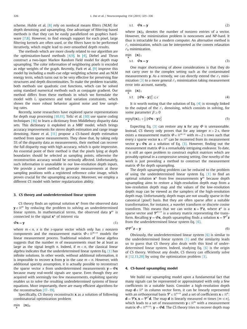
Sparsity as a prior could not guarantee that Eq. (8) could produceregularized results as it can only help us identify a solution from theinfinite possible solutions of the underdetermined linear system (6).Fig. 1(b) shows the upsampled result produced by Eq. (8). We canobserve that the depth surfaces suffer from fluctuation artifactswhich significantly lower the upsampling quality. To solve theproblem, we incorporate an additional total variation (TV) term forsmoothing the depth map while still preserving discontinuities. TheTV term is defined in l1 norm:

‖d‖TV ¼ ∑n

i ¼ 1ðj∇hðdðiÞÞjþj∇vðdðiÞÞjÞ ð9Þ

where ∇h;∇v denote the local horizontal and vertical gradients forpixel dðiÞ respectively. In practice, we find that l1 norm TV (alsoknown as anisotropic TV [23]) produces sharper boundaries than l2norm for our data sets. After adding this term to the objectivefunction in Eq. (8), we convert our final model into the followingunconstrained optimization problem:

mind

α‖d‖TVþβ‖Ψ Td‖1þ12 ‖y�Φd‖22 ð10Þ

where parameters α;β control the weights of the two regularizationterms. The regularized result of Eq. (10) is demonstrated in Fig. 1(c).Compared with the result of Eq. (8), the nasty artifacts are removedentirely and therefore the depth surfaces in Fig. 1(c) are rathersatisfactory.

ForΨ andΦ, we follow the patterns defined in [11]:Ψ representsa Daubechies Wavelet basis, while Φ samples the high-resolutiondepth map with canonical pixel basis. The term Φ is important forour depth upsampling application as Φ should satisfy the minimummeasurement requirement [24] deduced from CS theory. Strictlyspeaking, CS theory could not be directly applied to our modelwithout mathematical proofs because we add an extra TV term tothe standard CS model and thus our CS-based upsampling model(10) does not coincide with the standard CS model. However, we find

that our CS-based upsampling model shares the similar behaviorwith the standard CS model because both of them solve the under-determined linear system. Thus the factors that influence the finalresults of the standard CS model should also influence the resultingquality of our CS-based upsampling model. In the sequel, we willconduct experiments to verify the assumption and employ theconclusions of CS theory to discuss how to construct a satisfactoryΦ for accurate recovery.

5. Sampling data generation

This section describes how to construct the measurement matrixΦ used for depth upsampling (i.e. how to generate the samplingdata from a low-resolution depth map Dl and a registered high-resolution color image Ih) as the measurement matrixΦ is a specificmatrix that should satisfy the minimum measurement require-ments. In the following paragraphs, the sampling position informa-tion is denoted as a mask image Mh. If the pixel (i,j) is selected as asampling point, Mhði; jÞ ¼ 1; otherwise Mhði; jÞ ¼ 0. The samplingvalues are stored in a high resolution depth map Dh. Note that Dh isused for sampling purpose only, and it is not the final output of ourupsampling algorithm. The measurement matrix Φ and the mea-surements y can be easily constructed from Mh and Dh. Withoutlosing any generality, the upsampling factor for both horizontal andvertical directions is set as U. A pixel ði; jÞADl corresponds to a U�Upatch in the high resolution image space.

5.1. Minimal number of measurements

Both the compressive sensing problem Eq. (1) and our depthupsampling problem Eq. (6) consist in reconstructing an s-sparsevector from an underdetermined linear system. Although the sparsityassumption hopefully helps in identifying the original vector, it isunreasonable to expect that we can restore original vector from theobserved measurements with arbitrary number. Indeed, there is alower bound for the number of measurements. In other words, thenumber of measurements must be greater than the minimal numberof measurements; otherwise, no one could identify the originalvector. More importantly, the lower measurement number impliesthe larger upsampling rates for depth upsampling.

In literature, CS theory has proved that the mutual coherenceμðΦ;Ψ Þ between the sensing matrix Φ and the representationbasis Ψ determines the minimal number of measurements andμðΦ;Ψ ÞA ½1; ffiffiffi

np �.

μðΨ ;ΦÞ ¼ ffiffiffin

p � max1rk;jrn

j⟨ψ k;ϕj⟩j ð11Þ

Then, for a fixed signal f nARn whose coefficients are at most Snonzero entries in the basis Ψ , the CS theory [20] guarantees that

Fig. 1. The upsampling results of Eqs. (8) and (10). (a) Is the ground truth, (b) demonstrates the 8X upsampling result of Eq. (8), (c) shows the 8X upsampling result ofEq. (10). Compared (c) with (b), we can observe that there are nasty artifacts on the depth surfaces of (b).

L. Dai et al. / Neurocomputing 154 (2015) 325–336 327

select m measurements in the Φ domain uniformly at random; if

mZC � μ2ðΨ ;ΦÞ � S � logn ð12Þ

for some positive constant C, the solution of compressive sensing isexact with overwhelming probability. More specifically, it is shownthat the probability of success exceeds 1�δ if

mZC � μ2ðΨ ;ΦÞ � S � log nδ

� �ð13Þ

At last, we note that both the lower bound and the restorationquality for our depth upsampling problem are determined by thesensing partner of the sensing matrix Φ as the representation basisΨ are selected as the Daubechies Wavelet basis in advance.

To fight against the high mutual coherence between the mea-surement matrixΦ and orthogonal representation bases Ψ [25], it isnatural and reasonable to randomly map the depth values of lowresolution depth map Dl into the high resolution depth map Dh.Specifically speaking, in depth upsampling situation, a pixel ði; jÞADl

corresponds to a U�U patch in Dh. From this patch, we randomlyselect one sample with uniform distribution, and set their Mh valuesto 1 as follows:

DhðinUþs; jnUþtÞ ¼Dlði; jÞ s; t ¼ 1;…;U ð14Þ

5.2. Our sampling method

Although the random sampling scheme could reduce the mutualcoherence and therefore decreases the lower bound of measure-ments, the sampling scheme could not keep depth edges in the highresolution depth map as sharp as depth edges in the low resolutiondepth map. Instead, we manually select pixels around depth dis-continuities as sampling data points and add random samplingpositions in the homogeneous region to decrease the mutualcoherence μðΨ ;ΦÞ. As discussed previously, this procedure is essen-tial for the accuracy of the model. Since depth borders are not knownbefore upsampling, we will infer their positions and the correspond-ing measurements with the auxiliary information of the registeredcolor photo.

We first detect homogeneous regions and border regions in theoriginal depth map Dl with a simple thresholding scheme. A pixelp¼ ði; jÞADl is classified as ‘homogenous’ if its depth value DlðpÞsatisfies the following condition, otherwise it falls into the ‘border’region:

jDlðpÞ�DlðqÞjoλ; 8qANðpÞ ð15Þ

where NðpÞ is the 4-connected neighborhood of pixel p, and λ is adepth threshold value. We then map this region information to thehigh resolution image space.Mh;Dh in homogeneous and border regi-ons are computed successively. Our sampling method is quite differentfromHawe et al.'s work [11]. Their method relies on intensity edges forborder detection, since no depth information is available. We insteaduse Dl for rough region detection, and then incorporate edge informa-tion to compute Mh and Dh only in border regions, which helps todistinguish intensity edges and actual depth borders.

The procedure described above works well for small or mod-erate upsampling factors. However, when U reaches 16 or evenlarger, the generated sampling points would be too sparse in thehigh resolution image space to meet the minimum measurementrequirements [24]. We provide a simple hierarchical solution forlarge upsampling factors. Large U is decomposed into a set of smallfactors: U ¼ U1 � U2…Um. Then, starting from the low resolutiondepth map, the sampling data generation process is performed mtimes with small factors to get the final high resolution Mh and Dh.In practice, U¼16 are decomposed as 4�4 respectively, such thatthe number of the times m is kept as low as possible.

5.2.1. Sampling homogeneous regionsFor a homogenous pixel ði; jÞADl, its depth value is directly

mapped to a U�U homogenous patch in Dh as follows:

DhðinUþs; jnUþtÞ ¼Dlði; jÞ s; t ¼ 1;…;U ð16Þ

From this patch, we randomly select one or several sampleswith uniform distribution, and set their Mh values to 1. As statedin [25], this random selection helps to lower the mutual coherencebetween Ψ and Φ.

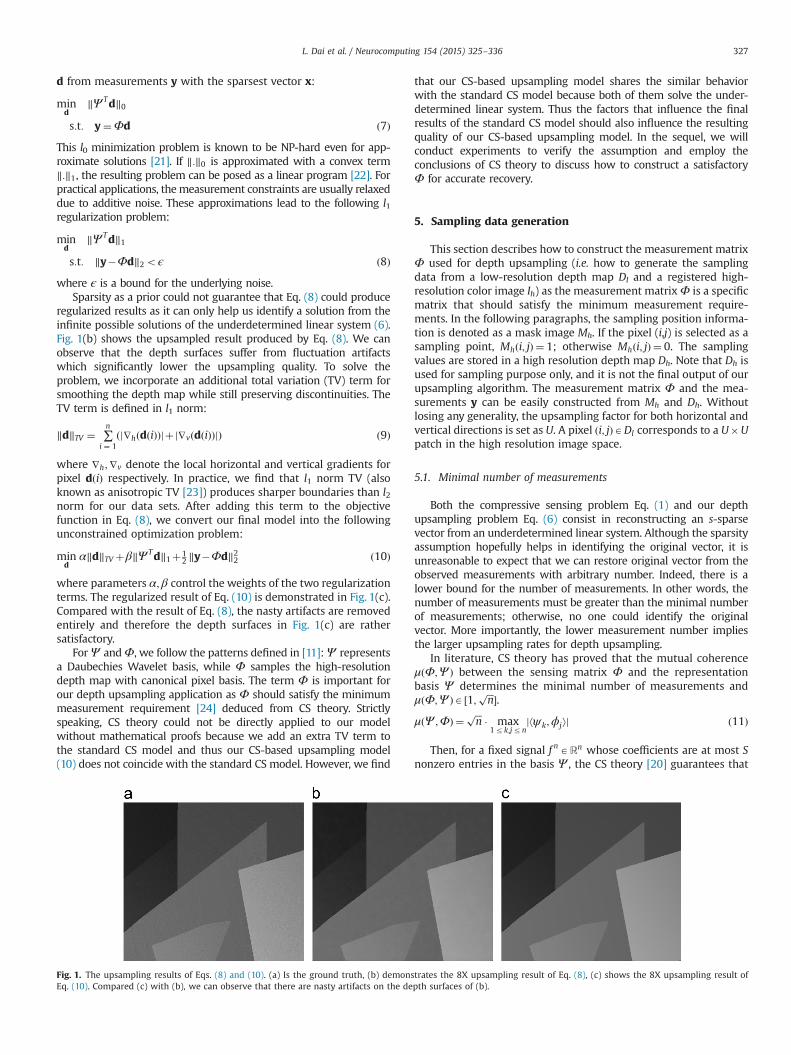
Fig. 2 shows the sampling data generation process for homo-geneous regions. We can observe that each pixel in the low resol-ution depth map (left image) corresponds to a 2�2 patch in the highresolution depth map (right image), where the pixels with the samecolor on either side denote the pixel-patch mapping. In the datageneration process, we randomly chose a red pixel in each patch andassign the corresponding depth in the low resolution depth map to it.

5.2.2. Sampling border regionsFor border pixels in Dl, their depth values are not reliable due to

the downsampling process, and directly mapping these pixels to Dh

would introduce significant sampling errors. We instead try to fillthese regions in Dh with homogenous depth values computed in theprevious step. The color image Ih should be considered in the fillingprocess. This problem can be posed as an inpainting problem with areference color image, and it shares some similarities with the occ-lusion handling problem in traditional stereo depth estimation [26].

Here, we provide a border region filling method based on theclassic Cellular Automata (CA) [27]. CA usually works on a regulargrid of cells, with finite states and local transition rules, which aresuitable for many image processing applications [28]. In mathema-tical terms, a cellular automaton is a triplet A¼ ðS;N; δÞ, where S is anon-empty state set. N is the neighborhood system, and δ : SN Oursolution is based on the CA model proposed by Vezhnevets andKonouchine [29]. Their model can propagate two labels to the fullimage. We employ this model for depth propagation and extend thelocal transition rules to respect the color distribution and the edgesin Ih, such that the propagation does not generate incorrect depthboundaries. Specifically, for each pixel p, our method stores a fourstate variable Sp ¼ ðDp;Θp; C

!p; EpÞ, where Dp denotes the depth of

pixel p, Θp is the ‘transition strength’ of pixel p, C!

p stands for thefeature vector of pixel p (i.e.the three dimensional vector of pixel p'scolor of Ih ) and Ep records Ih color edges detected by Canny filter.Without loss of generality, we assume Θp is bounded to [0, 1].

Initially, we assign Θp ¼ 1 for all the pixels with valid depthvalues, otherwise Θp ¼ 0. Moreover, if p lies on a color edge, Ep ¼ 1,otherwise Ep ¼ 0. After initialization, we collect all the pixels in theborder regions as a set P. The CA-based region filling algorithmupdates Spð8pAPÞ in an iterative manner according to the ruleslisted in Algorithm 1 which renews Sp from time t to tþ1, where f is

Fig. 2. An illustration of the sampling data generation process for homogeneousregions. Each pixel in the low resolution depth map (left image) corresponds to a2�2 patch in the high resolution depth map (right image), where the pixels withthe same color on either side denote the one-to-one mapping. The red color pixelsin each patch are randomly chosen and we assign the corresponding depths in thelow resolution depth map to them. (For interpretation of the references to color inthis figure caption, the reader is referred to the web version of this article.)

L. Dai et al. / Neurocomputing 154 (2015) 325–336328

a monotone decreasing function bounded to [0,1]:

f ð C!p1; C!

p2Þ ¼ 1�‖ C

!p1� C!

p2‖2ffiffiffi

3p ð17Þ

Algorithm 1. CA-based border region filling algorithm.

Input:State variables St

Output:

State variables Stþ1

1: for 8pAP do2: Dtþ1

p ¼Dtp

3: Θtþ1p ¼Θt

p

4: for 8qANðpÞ do5: if Ep ¼ ¼ 0 and Eq ¼ ¼ 1 then6: continue7: end if8: if f ð C!p; C

!qÞ �Θt

q4Θtp then

9: Dtþ1q ¼Dt

p

10: Θtþ1q ¼ f ð C!p; C

!qÞ �Θt

q

11: end if12: end for13: end for14: return Stþ1

In each iteration, the transition strength Θp is updated with theneighboring color information. The pixels lying on intensity edgesare only allowed to propagate depth information along the edge(Lines 5–7 in Algorithm 1). When no more pixel changes its state inthe iteration, the algorithm stops, and the output state variables areused to update Dh andMh. The pixels in P lying at color edges (i.e.thepixel pAE¼ fpjEp ¼ 1g) are all selected as sampling points. Thenthe subset P�fpjEp ¼ 0g of the remaining pixels are randomlyselected with a uniform distribution.

Using biological metaphor, the pseudocode listed above has anintuitive explanation. Since the depth values are discrete and have Ldifferent quantization levels, we can treat the depth assigning pro-cess which diffuses the depths from interpolating seeds to inter-polated pixels as growth and struggle for domination of L types ofbacteria. The culture media is limited to the border regions P. Thebacteria start to spread from the seed pixels and try to occupy all theborder regions P. We define the battlefront of different bacteria typesas the pixel set E and constrain that the warriors in the battlefrontshould not escape from the battlefield and invade the region of otherbacteria types (i.e.the if statement Ep ¼ ¼ 0 and Eq ¼ ¼ 1 in thepseudocode does). At each step, each bacteria p tries to attack itsneighbors NðpÞ. The attack force is defined by the attacker's transi-tion strength Θp and the distance between the feature vectorsC!

p1; C!

p2of attacker and defender. If the attack force is greater than

defender's strength, the defending pixel is conquered and its depthand strength are changed. The result of these local competitions isthat the strongest bacteria occupy the neighboring sites and gradu-ally spread over the border regions P.

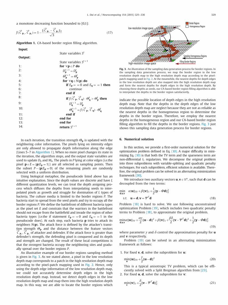
An illustrative example of our border regions sampling methodis given in Fig. 3. As we stated above, a pixel in the low resolutiondepth map corresponds to a patch in the high resolution depth mapaccording to the pixel-patch mapping used in Fig. 2. Hence, onlyusing the depth edge information of the low resolution depth map,we could not accurately determine depth edges in the highresolution depth map. Instead, we detect depth edges in the lowresolution depth map and map them into the high resolution depthmap. In this way, we are able to locate the border regions which

indicate the possible location of depth edges in the high resolutiondepth map. Note that the depths in the depth edges of the lowresolution depth map are neglect because they are not as reliable asthe nearest depths in the homogeneous region to determine thedepths in the border region. Therefore, we employ the nearestdepths in the homogeneous region and our CA-based border regionfilling algorithm to fill the depths in the border regions. Fig. 3 justshows this sampling data generation process for border regions.

6. Numerical solution

In this section, we provide a first-order numerical solution for theoptimization problem defined in Eq. (10). A major difficulty in mini-mizing Eq. (10) is that both the TV term and the sparseness term arenon-differential l1 regularizes. We decompose the original probleminto three subproblems with variable-splitting and quadratic penaltytechniques. For each subproblem, efficient solution is available. There-fore, the original problem can be solved in an alternatingminimizationframework [30].

We introduce two auxiliary vectors u; vARn, such that d can bedecoupled from the two terms:

mind;u;v

αju‖TV þβ‖v‖1þ12‖y�Φd‖22

s:t: u¼ d; v¼Ψ Td ð18ÞProblem (18) is hard to solve. We use following unconstrainedoptimization Problem (19), which includes two quadratic penaltyterms to Problem (18), to approximate the original problem.

mind;u;v

α‖u‖TV þαγ2‖u�d‖2þβ‖v‖1þ

βδ2‖v�Ψ Td‖2þ1

2‖y�Φd‖22

ð19Þwhere parameter γ and δ control the approximation penalty for uand v respectively.

Problem (19) can be solved in an alternating minimizationframework as follows:

1. For fixed v, d, solve the subproblem for u:

minu

‖u‖TV þγ2‖u�d‖2 ð20Þ

This is a typical anisotropic TV problem, which can be effi-ciently solved with a Split Bregman algorithm from [23].

2. For fixed u, d, solve the subproblem for v:

minv

‖v‖1þδ2‖v�Ψ Td‖22 ð21Þ

Fig. 3. An illustration of the sampling data generation process for border regions. Inthe sampling data generation process, we map the border region in the lowresolution depth map to the high resolution depth map according to the pixel-patch mapping used in Fig. 2. At the meanwhile, the nearest depths for depth edgesin the low resolution depth are also mapped into the high resolution depth mapand form the nearest depths for depth edges in the high resolution depth. Bychoosing these depths as seeds, our CA-based border region filling algorithm is ableto interpolate the depths in the border region satisfactorily.

L. Dai et al. / Neurocomputing 154 (2015) 325–336 329

The problem is well studied in CS literature. Using the simpleone-dimensional shrinkage operator, we can directly writedown its analytic solution.

v¼max Ψ Td�1δ;0

� �sgnðΨ TdÞ ð22Þ

3. Finally, for fixed u,v, solve the subproblem for d:

mind

αγ2‖u�d‖2þβδ

2‖v�Ψ Td‖2þ1

2‖y�Φd‖22 ð23Þ

This least square problem promises a closed-form solution:

d¼ KðαγuþβΨvþyÞ ð24Þwhere K ¼ ðαγIþβδIþΦTΦÞ�1 is a diagonal matrix.

Steps 1–3 are iteratively performed until the algorithm converges.For our upsampling problem on 1390�1110 images, stable resultscan be efficiently achieved within 200 iterations.

7. Experiments

In this section, we first describe a preprocessing step to register thedepth camera and conventional camera as the procedure is an essentialstep for following experiments. Second, the experiments’ parameterconfiguration and the evaluation index are presented. After that, wecompare the upsampling results of different sensing patterns anddiscuss the functions of different terms in Eq. (10). Last but not least,we conduct extensive experiments, including the synthesized data andthe real world date, to illustrate the upsampling ability of our method.

7.1. Depth map registration

Depth maps and theirs companion color images are capturedby different cameras, thus they do not registered well in reality. LetXd ¼ ðX;Y ; Z;1Þ denote the 3D homogeneous coordinates of thepixels of a depth map, and Xc ¼ ðr; c;1Þ represent the 2D homo-geneous coordinates of the companion high-resolution RGB imageof the depth map. We have the following projection relationshipabout Xd and Xc:

Xc ¼ sK½R j t�Xd ð25Þwhere s is a scale factor, K is the intrinsic parameters of the opticalcamera, R and t are the rotation and translation matrix whichdescribe the rotation and translation of the optical camera and thedepth camera.

We can use the well-known calibration method introduced byZhang [31] to calibrate the parameters of the two cameras. However,the depth camera could not capture textures as the RGB camera does.Instead of using the traditional visible textures, we can use a planarcalibration pattern which consists of holes for the reason that theseholes can be captured by both cameras. A similar method has beenused by Park et al. [9] to register depth maps and color images too.For the two calibrated cameras, we can project any points Xd whichare on the low-resolution depth map onto the high-resolution RGBimage by using Eq. (25). In this situation, the scaling term s is therelative resolution between the depth camera and the optical camera,in other words, it is the upsampling rate. For any point xt which is onthe low-resolution depth map with depth value dt, we can transformthe local coordinate of the depth camera ½xt ; dt ;1�T into the worldcoordinate Xd by the following equation:

Xd ¼ P�1t ½xt dt 1�T ð26Þ

where P�1t is the inverse of the 4�4 projective transformation Pt

which converts the world coordinate Xd into the local coordinate½xt dt 1�T of the depth camera.

7.2. Parameter configuration and evaluation index

In the sequent experiments, we quantitatively test our algorithmon the Middlebury stereo datasets [32], which provide both highresolution color images and ground truth depth maps, as well as thewell-known KITTI Vision Benchmark Suite. Specifically, for thesynthesized experiments illustrated in Section 7.4, we use ‘Books’,‘Dolls’, ‘Moebius’ and ‘Plastic’ images of the Middlebury datasetswhereas we randomly choose three depth images from the KITTIVision Benchmark Suite to perform real data upsampling. The testplatform is a PC with Intel i5 2.8GHz CPU and 4GB memory. Theupsampling performance of our method is rather stable whenλ;α;β; γ; δ are in the ranges ½2;5�; ½0:5;2�; ½0:5;1:5�; ½25;35�; ½25;35�,respectively. For convenience, we consistently keep the parametersetting λ;α;β; γ; δ of all the data sets used in the experimentsunchanged, where λ¼ 4:0;α¼ 1:0;β¼ 1:0; γ ¼ 32:0;δ¼ 32:0. Theupsampling factor U, in our experiments, varies from 2X to 16X,which covers the resolution range for most depth sensors. For agiven factor U, the ground truth depth map is downsampled by U tocreate the input depth data.

For performance evaluation, we need to explain the meaning ofgetting a satisfactory result with a high probability because CS theoryonly guarantees that we have a high probability (refer to Eqs. (12)and (13) to obtain an exact result. Performing hundred expe-riments for an image and accounting the number of satisfactoryresults is not a rational method to evaluate the performance of ourmethod. Instead of using this direct method, we evaluate the PSNRindex of an upsampling result, which quantifies the quality of aresult. We measure the quality of the upsampled results with peaksignal-to-noise ratio, often abbreviated PSNR, which is used tomeasure the ratio between the maximum possible power of a signaland the power of corrupting noise that affects the fidelity of itsrepresentation [33]. If our method gets a satisfactory result with ahigh probability, the upsampling result tends to has a large PSNRindex, otherwise, it should have a small PSNR index at most ofthe time.

7.3. Sampling pattern

A common doubt about our upsampling method is whether the CStheory can be applied to our depth upsampling model as an additionalTV term is added to the tradition CS restoration model (Eq. (7). Franklyspeaking, we do not offer a mathematical analysis for the model as thetraditional CS theory does and we think that a detailed mathematicalanalysis is out of the scope of this paper as we only target at providinga novel and practical depth upsampling method. However, theexperimental results in the sequel support the idea of that our depthupsampling model behaves as the traditional CS restoration model(Eq. (7) does.

A major difference between CS model and the traditional inter-polation methods is whether the quality of final results is heavilyaffected by the sampling pattern of observed data. To the best of ourknowledge, the sampling pattern of observed data plays a minor rolein the interpolation quality for the traditional interpolation methods.In other words, the final results only depend on the number ofinterpolating pixels. On the contrary, the observed data's samplingpattern completely determines the final results of CS model. i.e. forsome sampling patterns, the CS model could satisfactorily restore thefinal result from the observed data. For the other sampling patterns,the CS model fails to complete this task, even the number of observeddepths is the same in both situations. The reason is that, as we statedin Section 5.1, the minimal numberm of measurements is determinedby the mutual coherence μ2ðΨ ;ΦÞ, i.e.

mZC � μ2ðΨ ;ΦÞ � S � logn ð27Þ

L. Dai et al. / Neurocomputing 154 (2015) 325–336330

For uniform grid distribution, μðΨ ;ΦÞ ¼ 6. Whereas, in the ran-dom sampling distribution situation, μðΨ ;ΦÞ ¼ 2:5 which is smallerthan the mutual coherence value of the uniform grid distribution.

Fig. 4(c) and (d) illustrates the phenomenon for 8X upsampling,where we take two different sampling patterns (or distribution) withthe same sampling number. One distribution is the uniform grid,which is usually employed by the traditional interpolation methods.The other one is the random distribution generated by Eq. (14). Wecan observe that our CS based model is unable to interpolate themissing depths in the edges boundary for the uniform samplingpattern and successes to recovery the depths for random distribution.The behavior coincides with the prediction of the CS theory. Randomdistribution is still an inappropriate sampling pattern as it could notkeep the sharp depth edges. The shortcoming can be observedin Fig. 4(c). As a remedy, in Section 5.2, we proposed a novel hybridsampling pattern which randomly takes sample in homogeneousregions and deterministically the depths in border regions. Theresults is demonstrated in Fig. 4(d). Compared with previous twosampling patterns which are the deterministic sampling pattern (i.e.uniform grid) and random distribution (i.e.random sampling) respec-tively, the restoration result Fig. 4(e) of our hybrid sampling pattern isthe best among the three sampling patterns.

7.4. Evaluations using the Middlebury stereo datasets

Our algorithm (denoted as CS1) was implemented with Matlab.For comparison, four methods are selected: the bilateral-filtering

based method (denoted as Bilateral) [6], two MRF-based methods(denoted as MRF1, MRF2) [4,9] and the original CS-based method(denoted as CS2) [11]. For the first two methods, we implementedthem with Matlab, and the parameters were finely tuned. For CS2and MRF2, we directly use the source code provided by the authors.One thing needed to be clarified is that CS2 was not designed forthe upsampling problem. We provide the results to show that oursampling strategy is more suitable for the specific problem.

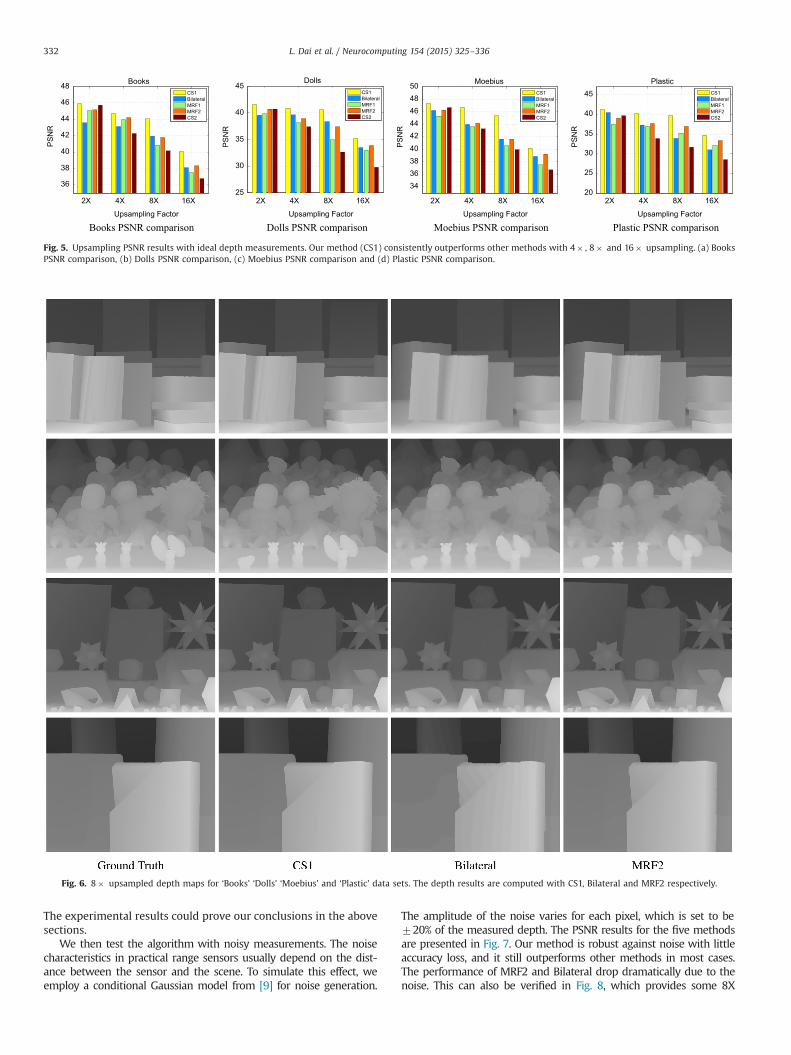
We first test the algorithm with ‘ideal’ low resolution depthmaps without noise corruption. The PSNR results for the fivemethods under various upsampling factors are presented in Fig. 5.Our algorithm works better under large upsampling factors. Itconsistently outperforms other methods with 2X, 4X, 8X and 16Xupsampling. MRF2 also gives overall satisfactory results in mostcases, while Bilateral and MRF 1 performs well under lowupsampling rates. Compared with the sampling method used inCS2, our sampling data generation method plays an important rolein high quality CS-based upsampling.

For the qualitative comparison of PSNR, we present some 8Xupsampled results computed by CS1, Bilateral and MRF2 methodsin Fig. 6. It can be seen that our method preserves sharp andaccurate depth boundaries during the upsampling process, whichdemonstrates the effects of the l1 regularization terms. We alsoown this achievement to our sampling method because ourmethod could generate accurate samples on boundaries with CA-based region filling method and the produced boundaries coincidewith the color edges of the high-resolution reference RGB photo.

Fig. 4. Sampling Pattern for 8X upsampling. (a) and (b) exhibit the guidance image and ground truth respectively, (c) demonstrates the uniform sampling, (d) illustrates therandom sampling, and (e) shows our sampling pattern. The sampling number is the same for the three distributions. We can observe that the restoration quality is verydifferent.

L. Dai et al. / Neurocomputing 154 (2015) 325–336 331

The experimental results could prove our conclusions in the abovesections.

We then test the algorithm with noisy measurements. The noisecharacteristics in practical range sensors usually depend on the dist-ance between the sensor and the scene. To simulate this effect, weemploy a conditional Gaussian model from [9] for noise generation.

The amplitude of the noise varies for each pixel, which is set to be720% of the measured depth. The PSNR results for the five methodsare presented in Fig. 7. Our method is robust against noise with littleaccuracy loss, and it still outperforms other methods in most cases.The performance of MRF2 and Bilateral drop dramatically due to thenoise. This can also be verified in Fig. 8, which provides some 8X

2X 4X 8X 16X

36

38

40

42

44

46

48

Upsampling Factor

PS

NR

Books

Books PSNR comparison

2X 4X 8X 16X25

30

35

40

45

Upsampling FactorP

SN

R

Dolls

Dolls PSNR comparison

2X 4X 8X 16X

343638404244464850

Upsampling Factor

PS

NR

Moebius

Moebius PSNR comparison

2X 4X 8X 16X20

25

30

35

40

45

Upsampling Factor

PS

NR

Plastic

Plastic PSNR comparison

Fig. 5. Upsampling PSNR results with ideal depth measurements. Our method (CS1) consistently outperforms other methods with 4� , 8� and 16� upsampling. (a) BooksPSNR comparison, (b) Dolls PSNR comparison, (c) Moebius PSNR comparison and (d) Plastic PSNR comparison.

Fig. 6. 8� upsampled depth maps for ‘Books’ ‘Dolls’ ‘Moebius’ and ‘Plastic’ data sets. The depth results are computed with CS1, Bilateral and MRF2 respectively.

L. Dai et al. / Neurocomputing 154 (2015) 325–336332

upsampled results computed by CS1, MRF2 and Bilateral methodsrespectively.

Our method has a great set of advantages. On the border regions,our cellular automata sampling method can produce sharp andaccurate edges. Therefore, we could obtain edge-preserving results.On the homogeneous regions, our sampling method could reduce

the mutual coherence between the measurement matrix Φ and theunitary matrix Ψ by random sampling. So our CS-based upsamplingalgorithm outperforms other methods. Although it is abnormal thatthe performance of our method is nearly same for lower upsamplingfactors such as 2X, 4X, 8X, the behavior is reasonable according to CStheory and the behavior does not imply fewer samples can keep

2X 4X 8X 16X25

30

35

40

45

Upsampling Factor

PS

NR

Books

Books PSNR comparison

2X 4X 8X 16X20222426283032343638

Upsampling Factor

PS

NR

Dolls

Dolls PSNR comparison

2X 4X 8X 16X

262830323436384042

Upsampling Factor

PS

NR

Moebius

Moebius PSNR comparison

2X 4X 8X 16X20

25

30

35

40

Upsampling Factor

PS

NR

Plastic

Plastic PSNR comparison

Fig. 7. Upsampling PSNR results with noisy measurements. Our method (CS1) still outperforms other methods in most cases. It shows robust behavior in noisy conditions.

Fig. 8. 8� upsampled depth maps with noisy measurements for ‘Books’ ‘Dolls’ ‘Moebius’ and ‘Plastic’ data sets. The depth results are computed with CS1, Bilateral and MRF2respectively.

L. Dai et al. / Neurocomputing 154 (2015) 325–336 333

reconstruction accuracy because the accuracy of our method decr-ease drastically at 16X upsampling factor and this tendency will bekept for larger U. For all the data sets, our algorithm produces thefinal results in 100 seconds, which is almost the same to the runningtime of CS2, but a bit slower than the MRF-based methods.

7.5. The performance characteristic of our method

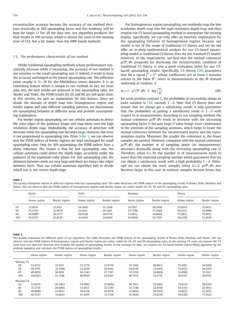
Unlike traditional upsampling methods whose performances con-sistently decrease while U increasing, the accuracy of our method isnot sensitive to the small upsampling rate U. Indeed, it tends to keepthe accuracy unchanged at the lowest upsampling rate. The inflectionpoint usually is U¼16 for the Middlebury stereo datasets. It is aninteresting feature which is unique to our method. In fact, for mostdata sets, the best results are achieved at low upsampling rates. For‘Books’ and ‘Dolls’, the PSNR results for 2X and 8X are still quite close.In this section, we give an explanation for this feature. Since wedivide the domain of depth map into homogeneous region andborder region and take different sampling patterns, we discriminatethe upsampling behavior at different areas and provide correspond-ing explanation.

For border region upsampling, we use cellular automata to detectthe color edges of the guidance image and map them onto the highresolution depth map. Undoubtedly, the accuracy of detection willdecrease while the upsampling rate becomes large. However, the erroris not proportional to upsampling rate. From Table 1, we can observethat the PSNR indices of border regions are kept unchanged for smallupsampling rates. Only for 16X upsampling, the PSNR indices have asharp reduction. The reason is that for low upsampling rate, thecellular automata could detect the depth edges accurately under theguidance of the registered color photo. For 16X upsampling rate, thedistances between seeds are very large and there are many color edgesbetween them. Thus our cellular automata algorithm fails to decidewhich one is the correct depth edge.

For homogeneous region upsampling, we randomly map the lowresolution depth map into the high resolution depth map and thenemploy our CS based upsampling method to interpolate the missingdepths. Specifically, we can only offer an heuristic explanation forthe upsampling behavior of homogeneous regions because ourmodel is out of the scope of traditional CS theory and we do notoffer an in-deep mathematical analysis for our CS-based upsam-pling model as traditional CS theory does for the standard CS model.However, in the experiments, we find that the mutual coherenceμðΨ ;ΦÞ proposed for disclosing the reconstruction condition oftraditional CS theory is also a good evaluation index for our CS-based upsampling model. Specifically, CS theory [20] guaranteesthat fix a signal f nARn whose coefficients are at most S nonzeroentries in the basis Ψ ; select m measurements in the Φ domainuniformly at random; if

mZC � μ2ðΨ ;ΦÞ � S � log nδ

� �ð28Þ

for some positive constant C, the probability of successfully obtain anexact solution to (18) exceeds 1�δ. Note that CS theory does notensure that we always get a satisfactory result; it only guaranteesthat the probability of getting a satisfactory result is 1�δ withrespect to m measurements. According to our sampling method, themutual coherence μðΨ ;ΦÞ tends to decrease with the increasingupsampling factor U because large U value brings more randomnessto the selection of the sampling positions, which helps to lower themutual coherence between the measurement matrix and the repre-sentation matrix. Moreover, the smaller the coherence is, the fewersamples are needed. However, compared with the mutual coherenceμðΨ ;ΦÞ, the number m of sampling pixels (or measurements)decreases drastically along with the increasing upsampling rate U.Therefore, when U¼16, the number m of measurements tends tolower than the expected sampling number which guarantees that wecan obtain a satisfactory result with a high probability 1�δ. Altho-ugh we can obtain the most samples when U¼2, μðΨ ;ΦÞ alsobecomes larger in this case. In contrast, samples become fewer, but,

Table 1The quality evaluation indices at different regions with four upsampling rates. The table illustrates the PSNR indices of the upsampling results of Books, Dolls, Moebius andPlastic. We can observe that the PSNR indices of homogenous regions and border region are rather stable for 2X, 4X and 8X upsampling rates.

Books Dolls Moebius Plastic

Homo region Border region Homo region Border region Homo region Border region Homo region Border region

2X 53.8519 33.1011 54.3603 31.3568 56.7017 38.2858 55.8319 35.60134X 51.1759 31.9870 53.3611 29.5401 55.7788 37.2668 54.3312 34.98868X 49.8089 30.3277 50.6128 28.0730 53.6832 34.8609 53.6831 33.605116X 45.5557 21.4138 41.4395 24.6849 47.0020 32.7195 50.6382 21.4138

Table 2The quality evaluation for different parts of our algorithm. The table illustrates the PSNR indices of the upsampling results of Books, Dolls, Moebius and Plastic. We canobserve that the PSNR indices of homogenous regions and border region are rather stable for 2X, 4X and 8X upsampling rates. In the missing TV rows, we remove the TVterm from our objective function and evaluate the quality of upsampling results. In the missing CA rows, we replace our CA-based border region filling algorithm by theuniform sampling and calculate the PSNR indices of upsampling results.

Homo region Border region Homo region Border region Homo region Border region Homo region Border region

Missing TV2X 53.0372 33.1011 53.7279 31.0730 55.7442 38.0812 55.4101 34.94564X 50.2701 31.7098 52.2636 29.1045 54.8139 37.0478 53.4155 34.23958X 49.6819 30.2011 50.3343 27.7391 53.1256 34.4606 52.8909 33.116716X 44.6423 21.1348 40.8926 24.3241 46.3314 32.1776 49.6787 20.9351

Missing CA2X 53.8519 26.5463 54.3603 25.9694 56.7017 33.3882 55.8319 29.05034X 51.1759 24.9265 53.3611 23.7245 55.7788 32.8109 54.3312 26.39128X 49.8089 22.0931 50.6128 20.4178 53.6832 28.3978 53.6831 23.201216X 45.5557 14.4655 41.4395 13.7329 47.0020 25.6259 50.6382 17.9143

L. Dai et al. / Neurocomputing 154 (2015) 325–336334

the minimal number of measurements also small. As a result, theprobability 1�δ of getting a satisfactory result is not changed verymuch for a wide range of upsampling.

It is also interesting to discuss the affect of the TV regularizationand our CA-based border region filling algorithm for depth upsam-pling because they are two novel terms which are introduced to theclassical compressive sensing model by us. In order to disclose theaffect of them, we remove the TV regularization from our samplingmodel and evaluate the quality of upsampling results at first. Afterthat, we substitute our CA-based border region filling algorithm withthe uniform sampling illustrated in Fig. 4(c) to reveal the function ofour CA-based border region filling algorithm. The quantitative resultsare reported in Table 2. Compared to Table 1, we can easily find thatthe TV regularization term mainly affects the upsampling quality ofhomogeneous regions. This is because the PSNR indices are signifi-cantly decreased in contrast to the PSNR indices in the border region.Different from the TV regularization term, our CA-based border regionfilling algorithm only affects the quality of upsampling results in theborder region. The reason is that the PSNR indices of homogeneousregions in the missing CA rows are same to the data in Table 1. If wecompare the PSNR indices of the border region in the missing TV rowsto PSNR indices in the missing CA rows, we can also observe that theCA-based border region filling algorithm heavily affects the finalupsampling results. However, it is not reasonable to say that the CA-based border region filling algorithm is more important than the TVregularization because the TV regularization is only designed tosmooth the depth values in the homogeneous region and the CA-based border region filling algorithm is only used to keep the sharpedges in the border region. In our algorithm, the two different termsare jointly exploited to improve the upsampling quality in thehomogeneous region and border region simultaneously.

7.6. Real world experiments

Lacking of 3D laser scanner, we use the standard database fromKITTI Vision Benchmark Suite [34]. All of the data is acquired by astandard station wagon with two color and grayscale video cameras.The accurate ground truth is provided by a Velodyne laser scanner. Wetake advantage of the laser scanner and companied color image toperform our experiments.

The KITTI database aims to offer people a challenging real-worldcomputer vision benchmarks for autonomous driving. However, thedatabase is not in preparation for stereo evaluation as Scharstein [35]did. It is a big challenge to use this KITTI Vision database forupsampling experiments, because all of the data is captured fromKarlsruhe streets and the obtained scenes are usually very large, thusthe object structures are relatively small in the pictures. Comparedwith the artificial in-door pictures used in state-of-the-art methods[4,6,9,11], it suffers from varied sensing noise. This situation demandsstrong denosing ability of upsampling algorithm.

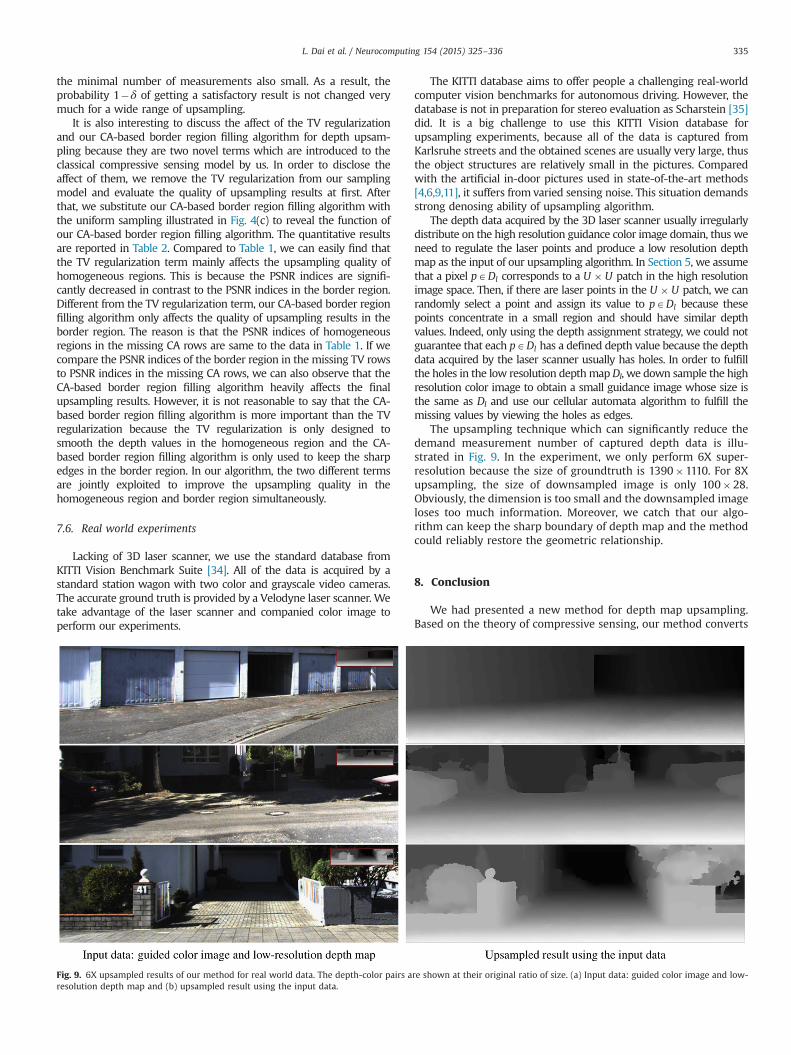
The depth data acquired by the 3D laser scanner usually irregularlydistribute on the high resolution guidance color image domain, thus weneed to regulate the laser points and produce a low resolution depthmap as the input of our upsampling algorithm. In Section 5, we assumethat a pixel pADl corresponds to a U � U patch in the high resolutionimage space. Then, if there are laser points in the U � U patch, we canrandomly select a point and assign its value to pADl because thesepoints concentrate in a small region and should have similar depthvalues. Indeed, only using the depth assignment strategy, we could notguarantee that each pADl has a defined depth value because the depthdata acquired by the laser scanner usually has holes. In order to fulfillthe holes in the low resolution depthmapDl, we down sample the highresolution color image to obtain a small guidance image whose size isthe same as Dl and use our cellular automata algorithm to fulfill themissing values by viewing the holes as edges.

The upsampling technique which can significantly reduce thedemand measurement number of captured depth data is illu-strated in Fig. 9. In the experiment, we only perform 6X super-resolution because the size of groundtruth is 1390�1110. For 8Xupsampling, the size of downsampled image is only 100�28.Obviously, the dimension is too small and the downsampled imageloses too much information. Moreover, we catch that our algo-rithm can keep the sharp boundary of depth map and the methodcould reliably restore the geometric relationship.

8. Conclusion

We had presented a new method for depth map upsampling.Based on the theory of compressive sensing, our method converts

Fig. 9. 6X upsampled results of our method for real world data. The depth-color pairs are shown at their original ratio of size. (a) Input data: guided color image and low-resolution depth map and (b) upsampled result using the input data.

L. Dai et al. / Neurocomputing 154 (2015) 325–336 335

the low resolution depth maps into a set of measurements, andthen formulates the upsampling task as a constrained optimiza-tion problem with data, smoothness and represent sparsenessconstraints. We validated our method with the Middlebury datasets, demonstrating that our method clearly outperforms previousmethods under large upsampling factors and noisy inputs.

Acknowledgements

This work was supported by National Natural Science Founda-tion of China (Nos. 61332017, 61331018, 91338202, and 61271430)).The authors would like to thank respected anonymous reviewersfor their constructive and valuable suggestions for improving theoverall quality of this paper.

References

[1] Y. Lei, M. Bennamoun, M. Hayat, Y. Guo, An efficient 3D face recognitionapproach using local geometrical signatures, Pattern Recognit. 47 (2) (2014)509–524.

[2] E. Rodolà, A. Albarelli, F. Bergamasco, A. Torsello, A scale independent selectionprocess for 3D object recognition in cluttered scenes, Int. J. Comput. Vis. 102(1–3) (2013) 129–145, ISSN 0920-5691.

[3] Y. Guo, F. Sohel, M. Bennamoun, M. Lu, J. Wan, Rotational projection statisticsfor 3D local surface description and object recognition, Int. J. Comput. Vis. 105(1) (2013) 63–86, ISSN 0920-5691.

[4] J. Diebel, S. Thrun, An application of Markov random fields to range sensing,in: Proceedings of Conference on Neural Information Processing Systems, MITPress, Cambridge, MA, 2005.

[5] J. Kopf, M.F. Cohen, D. Lischinski, M. Uyttendaele, Joint bilateral upsampling,ACM Transa. Graph. 26 (3), ISSN 0730-0301.

[6] Q. Yang, R. Yang, J. Davis, D. Nister´, Spatial-depth super resolution for rangeimages, in: IEEE Conference on Computer Vision and Pattern Recognition,2007. ISSN 1063-6919, 1–8.

[7] D. Chan, H. Buisman, C. Theobalt, S. Thrun, A noise aware filter for real-timedepth upsampling, in: Workshop on Multi-camera and Multi-modal SensorFusion Algorithms and Applications, Marseille, France, 2008.

[8] B. Huhle, T. Schairer, P. Jenke, W. Strasser, Fusion of range and color images fordenoising and resolution enhancement with a non-local filter, Comput. Vis.Image Underst. 114 (12) (2010) 1336–1345, ISSN 1077-3142.

[9] J. Park, H. Kim, Y. Tai, M.S. Brown, I. Kweon, High quality depth mapupsampling for 3D-TOF cameras, in: Proceedings of the 2011 InternationalConference on Computer Vision, IEEE Computer Society, Washington, DC, USA,2011. ISBN 978-1-4577-1101-5, 1623–1630.

[10] I. Tošić, B.A. Olshausen, B.J. Culpepper, Learning sparse representations ofdepth, IEEE J. Sel. Top. Signal Process. 5 (2011) 941–952.

[11] S. Hawe, K.D.M. Kleinsteuber, Dense Disparity Maps from Sparse DisparityMeasurements, IEEE Computer Society, Los Alamitos, CA, USA. ISBN 978-1-4577-1101-5, 2126–2133, 2011.

[12] E. Candès, J. Romberg, T. Tao, Robust uncertainty principles: exact signalreconstruction from highly incomplete frequency information, IEEE Trans. Inf.Theory 52 (2) (2006) 489–509, ISSN 0018-9448.

[13] D. Donoho, Compressive sensing, IEEE Trans. Inf. Theory 52 (4) (2006)1289–1306, ISSN 0018-9448.

[14] C. Tomasi, R. Manduchi, Bilateral Filtering for Gray and Color Images, in:Proceedings of the Sixth International Conference on Computer Vision, IEEEComputer Society, Washington, DC, USA, vol. 839, 1998. ISBN 81-7319-221-9.

[15] A. Buades, B. Coll, J.M. Morel, in: IEEE Conference on Computer Vision andPattern Recognition, vol. 2, vol. 2, 2005, pp. 60–65. ISSN 1063-6919.

[16] B.A. Olshausen, D.J. Field, Sparse coding with an overcomplete basis set: astrategy employed by V1? Vis. Res. 37 (1997) 3311–3325, ISSN 0042-6989.

[17] M. Figueiredo, R. Nowak, S. Wright, Gradient projection for sparse reconstruc-tion: application to compressed sensing and other inverse problems,IEEE J. Sel. Top. Signal Process. 1 (4) (2007) 586–597, ISSN 1932-4553.

[18] E.T. Hale, W. Yin, Y. Zhang, Fixed-point continuation for ℓ1-minimization:methodology and convergence, SIAM J. Optim. 19 (3) (2008) 1107–1130, ISSN1052-6234.

[19] Y. Wang, W. Yin, Sparse signal reconstruction via iterative support detection,SIAM J. Imaging Sci. 3 (3) (2010) 462–491, ISSN 1936-4954.

[20] E. Candès, M. Wakin, An introduction to compressive sampling, IEEE SignalProcess. Mag. 25 (2) (2008) 21–30, ISSN 1053-5888.

[21] S. Muthukrishnan, Data streams: Algorithms and Applications, Found. Trendsin Theoretical Computer Science, vol. 1, Now Publishers Inc., Hanover, MA,USA, 2005.

[22] S. Chen, D. Donoho, M. Saunders, Atomic decomposition by basis pursuit,SIAM Rev. 43 (1) (2001) 129–159, ISSN 0036-1445.

[23] T. Goldstein, S. Osher, The split Bregman method for L1-regularized problems,SIAM J. Imaging Sci. 2 (2) (2009) 323–343, ISSN 1936-4954.

[24] E. Candès, J. Romberg, Sparsity and incoherence in compressive sampling,Inverse Probl. 23 (2007) 969–985, ISSN 0266-5611.

[25] D.L. Donoho, X. Huo, Uncertainty principles and ideal atomic decomposition,IEEE Trans. Inf. Theory 47 (7) (2006) 2845–2862, ISSN 0018-9448.

[26] L. Wang, H. Jin, R. Yang, M. Gong, Stereoscopic inpainting: joint color anddepth completion from stereo images, in: IEEE Conference on ComputerVision and Pattern Recognition, 2008, pp. 1–8. ISSN 1063-6919.

[27] J.V. Neumann, Theory of Self-Reproducing Automata, University of IllinoisPress, Champaign, IL, USA, 1966.

[28] D. Popovici, A. Popovici, Cellular automata in image processing, in: 15thInternational Symposium on Mathematical Theory of Networks and Systems,2002.

[29] V. Vezhnevets, V. Konouchine, GrowCut: interactive multi-label N-D imagesegmentation by cellular automata, in: GraphiCon, 2005.

[30] Y. Wang, J. Yang, W. Yin, Y. Zhang, A new alternating minimization algorithmfor total variation image reconstruction, SIAM J. Imaging Sci. 1 (3) (2008)248–272, ISSN 1936-4954.

[31] Z. Zhang, A flexible new technique for camera calibration, IEEE Trans. PatternAnal. Mach. Intell. 22 (11) (2000) 1330–1334, ISSN 0162-8828.

[32] H. Hirschmüller, D. Scharstein, Evaluation of cost functions for stereo match-ing, in: IEEE Conference on Computer Vision and Pattern Recognition, 2007,1–8. ISSN 1063-6919.

[33] Q. Huynh-Thu, M. Ghanbari, Scope of validity of PSNR in image/video qualityassessment, Electron. Lett. 44 (13) (2008) 800–801, ISSN 0013-5194.

[34] A. Geiger, P. Lenz, R. Urtasun, Are we ready for autonomous driving?. The KITTIvision benchmark suite, in: IEEE Conference on Computer Vision and PatternRecognition, 2012, pp. 3354–3361. ISSN 1063-6919.

[35] D. Scharstein, R. Szeliski, A taxonomy and evaluation of dense two-framestereo correspondence algorithms, Int. J. Comput. Vis. 47 (1–3) (2002) 7–42,ISSN 0920-5691.

Longquan Dai received his B.S. degree in ElectronicEngineering from Henan University of Technology,China, in 2006. He received his M.S. degree in Electro-nic Engineering from Shantou University, China, in2010. Currently, he is working toward the Ph.D. degreein Computer Science at institute of automation, Chineseacademy of sciences, China. His research interests lie incomputer graphics, computer vision and optimization-based techniques for image analysis and synthesis.

Haoxing Wang is a Ph.D. candidate in the Sino-FrenchLaboratory (LIAMA) and National Laboratory of PatternRecognition (NLPR) at Institute of Automation, ChineseAcademy of Sciences. He received his B.S. and M.S.degrees in geographic information system from WuhanUniversity of Technology, China in 2006, and BeijingNormal University, China, in 2010, respectively. Hisresearch interests include photogrammetry, structurefrom motion techniques, optimization-based techni-ques for image analysis and synthesis.

Xiaopeng Zhang received his M.Sc. degree in Mathe-matics from Northwest University in 1987, and the Ph.D.degree in Computer Science from Institute of Software,Chinese Academy of Sciences (CAS), in 1999. He is aProfessor in the Sino-French Laboratory (LIAMA) and(National Laboratory of Pattern Recognition) at Instituteof Automation, CAS. His main research interests arecomputer graphics and pattern recognition. He receivedthe National Scientific and Technological Progress Prize(Second Class) in 2004. Xiaopeng Zhang is a member ofACM and IEEE.

L. Dai et al. / Neurocomputing 154 (2015) 325–336336