Deriving a Complete Type Inference for Hindley-Milner and Vector Sizes usingExpansionI

Axel Simona

a Technische Universitat Munchen, Lehrstuhl fur Informatik 2, Garching b. Munchen, Germany

Abstract

Type inference and program analysis both infer static properties about a program. Yet, they are constructed usingvery different techniques. We reconcile both approaches by deriving a type inference from a denotational semanticsusing abstract interpretation. We observe that completeness results in the abstract interpretation literature can beused to derive type inferences that are backward complete, a property akin to the inference of principal typings. Theresulting algorithm is similar to that of Milner-Mycroft, that is, it infers Hindley-Milner types while allowing forpolymorphic recursion. Although undecidable, we present a practical check that reliably distinguished typeable fromuntypeable programs. Instead of type schemes, we use expansion to instantiate types. Since our expansion operatoris agnostic to the abstract domain, we are able to apply it not only to types. We illustrate this by inferring the size ofvector types using systems of linear equalities and present practical uses of polymorphic recursion using vector types.

Keywords: type inference, abstract interpretation, principal typings, polymorphic recursion, expansion, completeanalysis, vector size inference, affine relations

1. Introduction

New computer languages are continuously designed, often in the form of domain-specific languages (DSLs). Onedesign aspect of a DSL is if the language should be statically typed and, if so, whether type inference should beused. Type inference is likely to be ruled out since addressing the special language features of a DSL in the typeinference may turn into an open-ended research problem. We therefore propose to apply the abstract interpretationframework [2] to constructively derive a type inference algorithm. The motivation is that a variety of abstract domainshave been developed over the years that can potentially be re-used for type inference, thereby going beyond Herbrandabstractions (type expressions containing type variables) commonly used in type inference. However, even if a set ofdomains are chosen and some type inference rules are put forth, different front-ends for the DSL might implement thetype inference slightly differently, thus infer different types for the same input and thereby accept a different set ofprograms. In order to address this issue, we propose to require the type inference to be backward complete, meaningthat it infers best (most general) types for every function and expression in the program. The benefit is that it is easyto decide if an implementation of the type inference is incorrect or imprecise (its inferred types are unsound or notthe best) and that type annotations are not required since there is no need to refine a type that is best (although theDSL may allow them for documentation purposes). These qualities also apply to inferences that deliver principaltypings [9], however, this notion requires that best types can be inferred in a bottom-up manner which is not possiblefor a Hindley-Milner type system [21]. We give a constructive way to create type inferences that infer best typesby building on a result from the abstract interpretation literature [15] that shows that, once certain properties hold, abackward complete type inference can be derived by simply abstracting the semantics of the language. However, thepresence of any branching construct (an if or a case statement) makes the derivation of a backward complete typeinference impossible, as illustrated by the following example:

ISupported by DFG Emmy Noether program SI 1579/1 and Microsoft SEIF 2013 grant. This work extends an earlier conference paper [18].URL: Axel.Simon@in.tum.de (Axel Simon)

Preprint submitted to Science of Computer Programming September 6, 2013

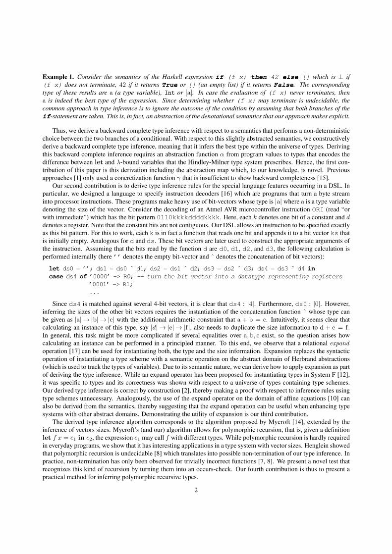
Example 1. Consider the semantics of the Haskell expression if (f x) then 42 else [] which is ⊥ if(f x) does not terminate, 42 if it returns True or [] (an empty list) if it returns False. The correspondingtype of these results are a (a type variable), Int or [a]. In case the evaluation of (f x) never terminates, thena is indeed the best type of the expression. Since determining whether (f x) may terminate is undecidable, thecommon approach in type inference is to ignore the outcome of the condition by assuming that both branches of theif-statement are taken. This is, in fact, an abstraction of the denotational semantics that our approach makes explicit.

Thus, we derive a backward complete type inference with respect to a semantics that performs a non-deterministicchoice between the two branches of a conditional. With respect to this slightly abstracted semantics, we constructivelyderive a backward complete type inference, meaning that it infers the best type within the universe of types. Derivingthis backward complete inference requires an abstraction function α from program values to types that encodes thedifference between let and λ-bound variables that the Hindley-Milner type system prescribes. Hence, the first con-tribution of this paper is this derivation including the abstraction map which, to our knowledge, is novel. Previousapproaches [1] only used a concretization function γ that is insufficient to show backward completeness [15].

Our second contribution is to derive type inference rules for the special language features occurring in a DSL. Inparticular, we designed a language to specify instruction decoders [16] which are programs that turn a byte streaminto processor instructions. These programs make heavy use of bit-vectors whose type is |a| where a is a type variabledenoting the size of the vector. Consider the decoding of an Atmel AVR microcontroller instruction ORI (read “orwith immediate”) which has the bit pattern 0110kkkkddddkkkk. Here, each k denotes one bit of a constant and ddenotes a register. Note that the constant bits are not contiguous. Our DSL allows an instruction to be specified exactlyas this bit pattern. For this to work, each k is in fact a function that reads one bit and appends it to a bit vector ks thatis initially empty. Analogous for d and ds. These bit vectors are later used to construct the appropriate arguments ofthe instruction. Assuming that the bits read by the function d are d0, d1, d2, and d3, the following calculation isperformed internally (here ’’ denotes the empty bit-vector and ˆ denotes the concatenation of bit vectors):

let ds0 = ’’; ds1 = ds0 ˆ d1; ds2 = ds1 ˆ d2; ds3 = ds2 ˆ d3; ds4 = ds3 ˆ d4 incase ds4 of ’0000’ -> R0; -- turn the bit vector into a datatype representing registers

’0001’ -> R1;...

Since ds4 is matched against several 4-bit vectors, it is clear that ds4 : |4|. Furthermore, ds0 : |0|. However,inferring the sizes of the other bit vectors requires the instantiation of the concatenation function ˆ whose type canbe given as |a| → |b| → |c| with the additional arithmetic constraint that a + b = c. Intuitively, it seems clear thatcalculating an instance of this type, say |d| → |e| → |f|, also needs to duplicate the size information to d + e = f .In general, this task might be more complicated if several equalities over a,b, c exist, so the question arises howcalculating an instance can be performed in a principled manner. To this end, we observe that a relational expandoperation [17] can be used for instantiating both, the type and the size information. Expansion replaces the syntacticoperation of instantiating a type scheme with a semantic operation on the abstract domain of Herbrand abstractions(which is used to track the types of variables). Due to its semantic nature, we can derive how to apply expansion as partof deriving the type inference. While an expand operator has been proposed for instantiating types in System F [12],it was specific to types and its correctness was shown with respect to a universe of types containing type schemes.Our derived type inference is correct by construction [2], thereby making a proof with respect to inference rules usingtype schemes unnecessary. Analogously, the use of the expand operator on the domain of affine equations [10] canalso be derived from the semantics, thereby suggesting that the expand operation can be useful when enhancing typesystems with other abstract domains. Demonstrating the utility of expansion is our third contribution.

The derived type inference algorithm corresponds to the algorithm proposed by Mycroft [14], extended by theinference of vectors sizes. Mycroft’s (and our) algorithm allows for polymorphic recursion, that is, given a definitionlet f x = e1 in e2, the expression e1 may call f with different types. While polymorphic recursion is hardly requiredin everyday programs, we show that it has interesting applications in a type system with vector sizes. Henglein showedthat polymorphic recursion is undecidable [8] which translates into possible non-termination of our type inference. Inpractice, non-termination has only been observed for trivially incorrect functions [7, 8]. We present a novel test thatrecognizes this kind of recursion by turning them into an occurs-check. Our fourth contribution is thus to present apractical method for inferring polymorphic recursive types.

2

a)u ∈P(U)

γ←→α

p ∈ P

f

yyf ]

u′ ∈P(U)γ←→α

p′ ∈ P

b)P(U)

∅

(a)≡P

⊥P

γ

αu⊆

p

vP

c)P(U)

∅

(a)≡P

⊥P

α

γu⊆ pvP

Figure 1: concrete/abstract transformers and monotone versus antitone abstraction

Overall, this paper makes the following four contributions:

• It observes that type inferences that are backward complete abstract interpretations exhibit the advantages as-sociated with the inference of principal typings, but that they are more general. We derive a backward com-plete type inference for the Hindley-Milner type system for which no principal typings exist by calculatingf ] = α f γ where f is the denotational semantics of an ML-like language, lifted to sets and f ] is thecorresponding type inference rule. We define the novel abstraction map α from value environments to Hindley-Milner type environments that encodes how λ- and let-bound variables differ in the way they are abstracted.

• We present a type inference for vector sizes that demonstrates how type inference can be extended by classicabstract domains found in program analysis.

• Our derivation instantiates function types using a domain-agnostic expand operator rather than type schemes.We illustrate the universality of this expand operator by extending the derived type system with the inference ofvector sizes.

• We present a novel test that turns all non-terminating behaviors that we have observed into an occurs check,thereby presenting a practical approach to inferring polymorphic recursive types.

After a primer on abstractions to types, Sect. 3 defines the denotational semantics that Sect. 4 abstracts to types,yielding a type inference algorithm. Section 5 sketches the inference of bit vectors sizes and presents an example forpolymorphic recursion (Sect. 5.2). Finally, Sect. 6 discusses our implementation and related work.

2. Overview of Abstracting into Types

We review the basics of backward completeness and how type inference can be described as an abstract interpre-tation. We then show how polymorphic types can be represented without type schemes.

2.1. Completeness in Abstract InterpretationFigure 1a) shows how the abstract interpretation framework [2] proposes to relate some abstract property p ∈ P

with several concrete properties u ⊆ U using an abstraction function α : P(U)→ P and/or a concretization functionγ : P → P(U). Given a complete partial order vP on P, the tuple 〈α, γ〉 forms a monotone Galois connection withα(u) vP p iff u ⊆ γ(p) as illustrated in Fig. 1b). We lift the program semantics that operates on the universe ofvalues U to P(U) and use it as the collecting semantics f . A monotone abstract transfer function f ] : P → P is asound approximation of f : P(U) → P(U) iff α f vP f

] α where (f g) = λx . f(g(x)). If α f = f ] αthen f ] is so-called backwards-complete [15] and the least fixpoint of f ] is the best possible (vP-smallest) abstractproperty p ∈ P, that is α(lfp⊆∅ (f)) = lfpvP

⊥P(f ]) where lfp≤S is the ≤-smallest fixpoint starting at S. Such an analysis

is called (abstract) complete [5, 15]. This paper derives a type inference for Hindley-Milner types that is abstractcomplete by calculating f ] = α f γ where f is the denotational semantics of an ML-like language, lifted to setsand f ] is the corresponding type inference rule. The so derived rules are backward complete if the additional property∀u1, u2 ∈P(U) . α(u1) = α(u2)⇒ α(f(u1)) = α(f(u2)) holds [15]. The latter property states that two inputs u1,u2 to a semantic rule f have no effect on its resulting type α(f(ui)) as long as their type α(ui) remains the same or,more intuitively, that the type system is not a dependent type system. The obtained backward complete inference rules

3

ensure that the inferred type for any program variable and expression is the most general type within the universe oftypes P which is often referred to as principal typing [9]. In our related work section, we will detail the differencebetween backward complete type inference and other definitions of principal typings [21].

2.2. Abstract Interpretation for TypesThe abstract interpretation framework is usually used for may-analyses that express possible behaviors of a pro-

gram. For instance, the abstract domain of intervals infers the may information x ∈ [2, 5] when approximating thepossible results of the Haskell expression if (f x) then 2 else 5. In contrast, type inferences are must-analyses that gather constraints that exclude certain program behaviors. For instance, inferring the type of the expres-sion if (f x) then ’11’ else ’10101’ yields a type error since the bit vectors ’11’ and ’10101’ giverise to two constraints, namely that the expression must be of type |2| and of type |5|, which is inconsistent. Note thatboth analyses may internally represent the states of the two branches with a = 2 and a = 5. However, when may-factsare inferred, the states are joined (yielding [2, 5] for the interval domain) whereas in the case where must-facts areinferred, the states are intersected (leading to an inconsistent constraint system). In other words, the union of twoprogram behaviors corresponds to an intersection in the abstract type domain. Analogously, the semantics of loopsthat is characterized by a least-fixpoint computation corresponds to a greatest-fixpoint computation on types. Thisis reflected by using an antitone Galois connection 〈α, γ〉 where p vP α(u) iff u ⊆ γ(p) as illustrated in Fig. 1c).The antitone relation between concrete and abstract domain is chosen to reflect the difference between type systemsand standard program analysis [1]. It is also possible to simply flip the abstract lattice upside down in which case thenumber of constraints grows with the number of program behaviors. This view has also been taken in the literature[14]. In this paper we chose the antitone view since commonly known abstract domains can be reused for type in-ference without flipping their join and meet operations. For instance, Herbrand structures that we use for types havepreviously been used to infer possible instantiations in Prolog programs [6]. Moreover, for vector sizes we use theaffine domain [10] that has previously been used to infer equality relations between numeric program variables.

2.3. Representing Polymorphism without Type SchemesLet X denote the set of program variables. For simplicity, we assume that variables at binding sites (λ- and let-

bindings) are pair-wise different. The Hindley-Milner type system assigns, to each variable x ∈ X, a type term rangingover a binary function symbol · → ·, data constructors and type variables. Additionally, variables at let-declarationsare usually associated with a type scheme which states which type variables may be instantiated. Due to the ability toinstantiate let-bound variables, these are called “polymorphic” whereas λ-bound variables are called “monomorphic”.However, this is overly simplistic, as illustrated by our running example, an elaborate identity function:

Example 2. The program let f = λx . let g = λy . x in g g in f yields the following type environment whenanalyzing x in λy . x:

f 7→ ∀a . a→a, x 7→ a, g 7→ ∀b .b→a, y 7→ b

Here, the type variable a is instantiated when using f (thus f is “polymorphic”) but not instantiated when using g.

Instead of type schemes that specify which type variables to instantiate, we will define an abstraction map αXM forwhole environments in which all type variables are implicitly ∀-quantified, resulting in the following types for Ex. 2:

f 7→ a→a, x 7→ a, g 7→ b→a, y 7→ b

As indicated in the example, using g requires that only the type variable b is instantiated to a fresh variable. Inorder to clarify how to instantiate the types above, we define a pre-order on X, with x 4 y if x is in scope of y, thatis, when y is bound by λy . e1 or by let y = e2 in e3 then ei may contain x. In the more general case of allowingbinding groups of the form letx = . . . ; y = . . . in . . ., both x 4 y and y 4 x hold since they are visible in eachother’s body. Let x ≺ y abbreviate y 64 x ∧ x 6= y. In the example, the ordering of the variables is f ≺ x ≺ g ≺ y.Furthermore, let Xλ ⊆ X denote the set of λ-bound variables, here x, y ∈ Xλ, f, g ∈ X \ Xλ. Instantiating the typeof u ∈ X \ Xλ substitutes fresh variables for all variables in the type of u that do not also occur in v ≺ u. The typeschemes can thus be recovered through a traversal starting at the ≺-smallest variable and generating type schemes ateach variable u ∈ X \ Xλ for all as-of-yet unquantified variables. Note, though, that the analysis we derive nevercreates any type schemes and but computes which variables to instantiate on-the-fly using 4 and Xλ.

This concludes the preliminaries for deriving a complete type inference. We now define the concrete semantics.

4

S[[·]] : E→ (X→ U⊥)→ U⊥S[[x]] ρ = ρ(x)

S[[λx . e]] ρ = ↑UF(λv .S[[e]] (ρ[x 7→ v]))

S[[e1 e2]] ρ = (v1 ∈F ? (v2 ∈W ? Ω : ↓UF(v1)v2) : Ω) where vi = S[[ei]] ρ for i = 1, 2

S[[let x = e in e′]] ρ = (v ∈W ? Ω : S[[e′]] (ρ[x 7→ v])) where v = lfp⊥Uλv .S[[e]] (ρ[x 7→ v])

S[[C e1 . . . en]] ρ = (v1 ∈W ? Ω : . . . (vn ∈W ? Ω : if δU(C v1 . . . vn) 6= ∅then ↑UA(C v1 . . . vn) else Ω) . . .) where vi = S[[ei]] ρ for i ∈ [1, n]

S[[case es of C x1 . . . xn : et; ee]] ρ = (vs ∈A ? if δU(↓UA(vs)) ∩ (∪δU(C v′1 . . . v′n) | v′i ∈ U) = ∅ then Ω else

if ↓UA(vs) = C v1 . . . vn then S[[et]] ρ[x1 7→ v1, . . . xn 7→ vn] else S[[ee]] ρ

: Ω) where vs = S[[es]] ρ

Figure 2: standard denotational semantics for e ∈ E

3. Syntax and Semantics

Before we give a semantic meaning to types, we commence by defining the syntax and semantics of an extendedλ-calculus. We mainly follow Milner [13] but add algebraic data types. Let x ∈ X and let C ∈ C be the n-aryconstructor of some algebraic data type. The set of expressions E is given by the following grammar:

e ∈ Ee ::= x | λx . e | e1 e2 | let x = e in e′

| C e1 . . . en | case es of C x1 . . . xn : et; ee

Here, the standard constructs of the λ-calculus are extended by a let-construct that allows x to be recursivelyused in e (x is in scope in e). The second line defines values in form of constructors with n arguments and a test thatmatches the value of the scrutinee es against the constructor C and, if successful, evaluates the “then”-branch et in anenvironment where xi is bound to the ith value of the constructor. If the match fails, the “else”-branch ee is evaluated.For the sake of presentation, we set C = Cons,Nil ∪ Z, for lists and integers.

Evaluating an expression may terminate with a type error. For instance, it is a type error if e1 ∈ E in the applicatione1 e2 does not evaluate to a λ-expression. In contrast, evaluating let f = λx . f (Cons 0 x) in f Nil may result ina heap overflow error. The aim in type checking a program is to guarantee the absence of type errors but the ambitionis not as high as proving the absence of other run-time errors. We now give a formal semantics to e ∈ E.

3.1. SemanticsLet S⊥ := S∪⊥Swhere⊥S /∈ S denotes an undefined value or a non-terminating evaluation. The denotational

standard semantics evaluates e ∈ E to a program value U⊥ where U is a sum of constructors terms A, functions F andthe set ω where ω, the wrong value, denotes a type error. It is defined as follows:

U := A + F + WF := U→ U⊥A := C v1 . . . vn | vi ∈ UW := ω

We construct values of type U from a value in D = A,F,W using the injection functions ↑UD(·) : D → U (thus,↑UD (x) is analogous to a Haskell/ML constructor of the algebraic data type U that wraps D). Conversely, define anextraction function ↓UD(·) : U⊥ → D⊥ with ↓UD(↑UD(v)) = v for all v ∈ D and ↓UD(·) = ⊥U otherwise. For brevity, letΩ =↑UW(ω) ∈ U denote the error value. We define the following C-like conditional to test if v ∈ U originated in D:

(v ∈D ? v1 : v2) =

v1 if v =↑UD(d) for some d ∈ D⊥U if v = ⊥Uv2 if otherwise

5

C[[·]] : E→P((X→ U⊥)→ U⊥)

C[[x]] = λρ . ρ(x)C[[λx . e]] = λρ . ↑UF(λv . S(ρ[x 7→ v])) | S ∈ C[[e]]C[[e1 e2]] = λρ . (S1ρ∈F ? (S2ρ∈W ? Ω : ↓UF(S1ρ)S2ρ) : Ω) | Si ∈ C[[ei]], i = 1, 2

C[[let x = e in e′]] = λρ . (v ∈W ? Ω : S′(ρ[x 7→ v])) | S′ ∈ C[[e′]] ∧ v ∈ V where V = lfp⊥U

λv . S(ρ[x 7→ v]) | S ∈ C[[e]]C[[C e1 . . . en]] = λρ . (S1ρ∈W ? Ω : . . . (Snρ∈W ? Ω : if δU(C S1ρ . . . Snρ) 6= ∅

then ↑UA(C S1ρ . . . Snρ) else Ω) . . .) | Si ∈ C[[ei]], i ∈ [1, n]C[[case es of C x1 . . . xn : et; ee]] := λρ . if @a .↑UA(a)=Ssρ ∨ δU(↓UA(Ssρ)) ∩ (∪δU(C v′1 . . . v

′n)|v′i ∈ U)=∅

then Ω else Stρ[x1 7→ v1, . . . xn 7→ vn]

| δU(↓UA(Ssρ)) ∩ δU(C v1 . . . vn) 6= ∅ ∧ vi ∈ U ∧ Ss ∈ C[[es]] ∧ St ∈ C[[et]]∪ λρ . if @a .↑UA(a)=Ssρ ∨ δU(↓UA(Ssρ)) ∩ (∪δU(C v′1 . . . v

′n)|v′i ∈ U)=∅

then Ω else Seρ | Ss ∈ C[[es]] ∧ Se ∈ C[[ee]]Figure 3: collecting semantics for e ∈ E, with case-statements being abstracted

The evaluation of an expression uses a value environment ρ ∈ X→ U⊥ that binds program variables X to valuesU⊥ = U∪⊥P. Choose x, y ∈ dom(ρ) such that x 6= y. An updated environment ρ′ = ρ[x 7→ v] ∈ X→ U⊥ obeysρ′(x) = v and ρ′(y) = ρ(y). A variable x is removed from ρ by projection, written ρ′ = ∃x(ρ), where ρ′(y) = ρ(y).

For the sake of defining the semantics of the language in a denotational way, we introduce fixpoint computationsand an order on values. Given a complete partial order 〈L,v〉 and a monotone function ψ : L → L, define theleast-fixpoint lfpv⊥ψ to be thev-smallest element l ∈ L with⊥ v l and ψ(l) v l. Define the partial order on valuesv ∈ U⊥ as follows: ⊥U v for all v ∈ U⊥. Moreover, f1 f2 if fi =↓UF(vi) 6= ⊥U for i = 1, 2 and f1(v) f2(v)for all v ∈ U. Also, C v1

1 . . . v1n C v2

1 . . . v2n if C vi1 . . . v

in =↓UA(vi) for i = 1, 2 and v1

k v2k for all k ∈ [1, n].

The denotational semantics S[[e]] ∈ (X → U⊥) → U⊥ of an expression e ∈ E is defined in Fig 2. Here, theconditional statement is used in two ways: Firstly, (v ∈D ? . . . ↓UD (v) . . . : Ω) is used to test if v ∈ U is in factelement of D and then to extract this element ↓UD(v) ∈ D while returning the type error Ω otherwise. Secondly, if avalue v is merely required not to be a type error, the statement (v ∈W ? Ω : . . .) is used which returns Ω if v is atype error. Note that both conditionals evaluate to ⊥U if v = ⊥U and, hence, the definition of e1 e2 returns ⊥U if e2 isundefined which gives the language a call-by-value semantics.

User-defined data types are given by the function δU : C×U∗ →P(∆) that maps a constructor and its argumentsto a set of data types ∆, to be defined later. For instance, δU(42) = Int, δU(Nil) = [Int], [[Int]], . . . andδU(Cons ↑UA(42) ↑UA(Nil)〉) = [Int]. Applying a constructor C ∈ C to arguments v1, . . . vn is a type error ifδU(C v1 . . . vn) = ∅, that is, if no matching user-define data type exists. Analogously, for case-statements, the valuevs of the scrutinee es must not only be a constructor term A but also share possible data types δU(↓UA(vs)) with theconstructor C. Here,

⋃δU(C v′1 . . . v

′n) | v′i ∈ U computes the possible data types that can be constructed using C.

3.2. Collecting SemanticsIn program analysis, every abstract value (here: a type) represents many concrete values. In order to relate a type

with a set of values, we lift the semantics S[[e]] : (X → U⊥) → U⊥ of an expression e ∈ E to a collecting semanticsC[[e]] : P((X → U⊥) → U⊥). We lift each rule of the standard semantics in Fig. 3 to work over sets by convertingeach rule S[[e]] ρ = . . .S[[e′]] . . . to C[[e]] = λρ . . . . S . . . | S ∈ C[[e′]], resulting in the rules in Fig. 3. The onlyexception is the case-statement for which the collecting semantics is a proper abstraction of the standard semantics.Here, the collecting semantics returns two function sets, one that always returns et and one that always returns ee.The test is further abstracted to ensure that the denotation does not depend on the actual value of es. Section 4.8will illustrate that this abstraction is required to derive a complete abstraction to types. Note that the evaluation of etrequires that the variables x1, . . . xn are bound to some value. We chose all values C v1 . . . vn that belong to the samedatatype as the value of es. This concludes the discussion of syntax and semantics.

6

4. Abstraction to Types

This section defines types, abstractions for (environments of) values, and finally derives the type inference algorithm.

4.1. Monomorphic and Polymorphic TypesThe underlying idea of types is to assign a type expression t ∈ M (or simply “type”) to a value that is calculated

in a program. Types in the context of the language E are defined as follows:

D t1 . . . tm ∈ ∆ algebraic data typest ∈ M monomorphic type expressionst ::= t1 → t2 | D t1 . . . tm

Here, the types of values that are not functions are given by some user-defined set of algebraic data types ∆ ⊂M.For the sake of simplicity, we fix ∆ = Int ∪ [t] | t ∈M. The definition of monotypes thus simplifies as follows:

t ∈ M monomorphic type expressionst ::= t1 → t2 | Int | [t]

During inference, and later also for polymorphic types, it is necessary to allow type variables v ∈ V to occur in atype expression, giving rise to polymorphic type expressions:

a,b, . . . ∈ V type variablest ∈ P polymorphic type expressionst ::= a | b | . . . | t1 → t2 | Int | [t]

The purpose of type variables is to act as a placeholder for other type expressions. Replacing type variables int ∈ P by another type expression creates an instance of t. The set of ground instances are those that contain no moretype variables and is given by ground:

ground : P→P(M)

ground(t) = σt ∈M | σ ∈ V →M

Here, σ ∈ V → M is a substitution that replaces type variables by monomorphic types. We define a partial or-der vP on t1, t2 ∈ P such that t1 vP t2 iff ground(t1) ⊆ ground(t2). Let t1≡Pt2 iff ground(t1) = ground(t2),that is, t1 is equal to t2 modulus the renaming of type variables. We use P⊥≡P

to denote the set of ≡P-equivalenceclasses of terms augmented with ⊥P. Then

〈P⊥≡P,vP, lca,gci, (a)≡P ,⊥P〉

is a complete lattice with join lca, meet gci, top element (a)≡P and a bottom element ⊥P with ⊥P vP t vP (a)≡P

for all elements t ∈ P⊥≡P. Here, (t)≡P denotes the ≡P-equivalence class of t ∈ P. The greatest common instance

t = gci(t1, t2) is calculated using unification [11]: Rename the variables in ti, giving t′i, such that t′1, t′2 do not

share any variables and t′i≡Pti for i = 1, 2. Then t = (σt′1)≡P if the most general unifier σ = mgu(t′1, t′2) exists

and t = ⊥P otherwise. For example, gci([a] → [Int], [Int] → b) = [Int] → [Int] = σ([a] → [Int]) withσ = mgu([a] → [Int], [Int] → b) = a/Int,b/[Int]. The dual operation lca : P × P → P calculates the leastcommon anti-instance [11]. For instance, lca([Int] → a, [[Int]] → a) = [b] → a. Note that lca preserves typevariables when they occur in compatible locations. In abuse of syntax, we also use lca : P(M)→ P ∪ ⊥P on setsof monotypes with lca(∅) := ⊥P. The relationship between sets of monomorphic type expressions and polymorphictype expressions can now be described by the following Galois insertion1 that uses lca on sets as α and a slightlyextended ground function of type ground : P⊥≡P

→P(M) as γ with ground(⊥P) := ∅:

〈P(M),⊆,∪,∩,M, ∅〉ground←lca

〈P⊥≡P,vP, lca,gci, (a)≡P ,⊥P〉

Given the ability to transform a set of types into a polymorphic type, it remains to show how to abstract a value toa set of types.

1A Galois insertion is a Galois connection where γ is injective which we ensure by factoring the abstract type lattice into equivalence classes.

7

αM : U⊥ →P(M)

αM(⊥U) = MαM(↑UA(c)) = Int if c ∈ Z

αM(↑UA(Cons l ll)) = [t] | t ∈ αM(l) ∩ αM(ll)

αM(↑UA(Nil)) = [t] | t ∈MαM(↑UF(f)) = t1 → t2 | v1 ∈ U∧

v2 = f(v1)∧ti ∈ αM(vi)

αM(Ω) = ∅

γM : M→P(U⊥)

γM(Int) = ⊥U ∪ ↑UZ(c) | c ∈ ZγM([t]) = ⊥U ∪ ↑UA(Nil) ∪

↑UA(Cons l ll) | l ∈ γM(t) \ ⊥U∧ll ∈ γM([t]) \ ⊥U

γM(ta → tr) = ⊥U ∪ ↑UF(f) | f ∈ U→ U⊥∧∀v ∈ γM(ta) \ ⊥U .f(v) ∈ γM(tr)

Figure 4: abstracting and concretizing values to types

4.2. Relating Values and TypesThe basic ingredients to relating program values and types are the functions αM : U⊥ → P(M) and γM : M →

P(U⊥) in Fig. 4 that map a single value to the corresponding set of types and a single type to the correspondingsets of values, respectively. For instance, αM(↑UA (Nil)) = [Int], [Int → Int], . . . which can be turned into apolymorphic type lca(αM(↑UA(Nil))) = [a]. In fact, these definitions encapsulate the definition of the user-defineddata types and thus allow us to give a formal definition of δU that mapped a constructor expression datatype:

Definition 1. The map δU : C×U∗ → ∆ of user-defined datatypes is defined δU(C v1 . . . vn) = αM(↑UA(C v1 . . . vn)).

Observe that lifting the functions in Fig. 4 to accept sets, that is, λu .⋂u∈u αM(u) and λt .

⋃t∈t γM(t) yields an

(antitone) Galois connection for single variables. The next section addresses how to abstract whole environments.

4.3. Relational Abstraction to TypesThe previous section illustrated how values of variables can be abstracted into types. While it is straightforward

to lift this abstraction point-wise to an environment, it is also incorrect:

Example 3. Consider the type environment when evaluating 42 in (λid . (λy . 42) id) (λx . x). At this point, λx . xhas been passed to id and to y. Applying αM point-wise gives [id 7→ T, y 7→ T ] where T = αM(λx . x) = Int→Int, [Int] → [Int], . . .. Thus, under this abstraction, id and y may have different types, that is, [id 7→ (a →a)≡P , x 7→ (a→a)≡P ] = [id 7→ a→a, x 7→ b→b]. This is incorrect, since y and id always observe the same value.

In order to state that two variables must have the same type, we represent an environment as a set of vectors oftypes. For instance, an environment [x 7→ a, y 7→ a] is represented by the set of vectors 〈t, t〉 | t ∈ M whereas[x 7→ a, y 7→ b] is represented by 〈t1, t2〉 | t1, t2 ∈ M. This abstraction preserves the relation between differentvariables and is therefore called relational.

Since vectors representing types of variables vary in length, depending on the number of variables in scope,we construct them as maps P(X → M) from program variables X to a type M, just like the maps for concreteenvironments ρ : X → U. For any fixed X, we interpret P(X → M) as X-indexed vectors P(MX). As such,they form a complete lattice 〈P(X → M),⊆,∪,∩, [x 7→ t]x∈X,t∈M, ∅〉. Vectors of polymorphic types are definedanalogously as maps from X to P but with the addition of identifying vectors that are equal modulus renaming ofvariables, written (X→ P)≡P , and the addition of a bottom element ⊥P. The resulting set forms the complete lattice

〈(X→ P)⊥≡P,vP , lca,gci, [x 7→ (a)≡P ]x∈X,⊥P〉

with join lca and meet gci defined below. Here vP denotes the conjunction of the point-wise lifting of the relationvP on polymorphic type expressions with ⊥PvP t for all t ∈ (X→ P)⊥≡P

. Note that the top element [x 7→ (a)≡P ]x∈Xmaps each x to a different type variable since two (a)≡P represent different equivalence classes. The join gci andmeet lca is calculated by interpreting the vector 〈t1, . . . , tn〉 as a single type t1 → . . .→ tn, applying gci (resp. lca),and converting the result back to a vector. Since relations within the type t1 → . . . → tn are preserved, the relationsbetween t1, . . . tn are preserved. We consider an example that contrasts vector and point-wise application of lca:

8

P(X→ U⊥)γXM←αXM

P(X→M)ground←lca

(X→ P)⊥≡P

f

yyf ]M

yf ]PP(X ∪ κ → U⊥)

γXM←αXM

P(X ∪ κ →M)ground←lca

(X ∪ κ → P)⊥≡P

Figure 5: our approach to abstracting denotational semantics

Example 4. Suppose two identifiers f, g can take on the following two monotypes ~t1,~t2 ∈M〈f,g〉:

〈Int→(Int→ [Int])→Int,Int→(Int→ [Int])→ [Int]〉〈Int→([Int]→Int)→ [Int],Int→([Int]→Int)→ [[Int]]〉

Replacing the comma by a function type symbol→, applying lca and replacing→ again by a comma yields:

〈Int→a→c,Int→a→ [c]〉

This result is an anti-instance since applying σ1 = a/Int → [Int], c/Int yields the first row and σ2 =a/[Int]→Int, c/[Int] the second row. By way of contrast, applying lca point-wise to ~t1 and ~t2, that is, computing〈lca(~t1(f),~t2(f)), lca(~t1(g),~t2(g)〉 ∈ Pf,g results in the anti-instance

〈Int→a→c,Int→b→ [d]〉

which is not the least-common anti-instance as it can be instantiated to 〈Int→a→c, Int→a→ [c]〉.

In order to account for the bottom element ⊥P in (X → P)⊥≡Pwe define lca(⊥P, t) = lca(t,⊥P) = t and

gci(⊥P, t) = gci(t,⊥P) = ⊥P. We lift the lca operation to sets, allowing us to relate polytype environments withtheir corresponding monotype environments, as given by the following Galois insertion:

〈P(X→M),⊆〉ground←lca

〈(X→ P)⊥≡P,vP 〉

In this context, we assume that lca(∅) = ⊥P. We lift ground : P⊥≡P→P(M) to vectors (X→ P)⊥≡P

as follows:

ground : (X→ P)⊥≡P→P(X→M)

ground(⊥P) = ∅ground(〈t1, . . . tn〉) = 〈σt1, . . . σtn〉 ∈M | σ ∈ V →M

Thus ground(〈a,b, Int〉) = 〈t1, t2, Int〉 | t1 ∈ M, t2 ∈ M whereas ground(〈a→ Int, a〉) = 〈t→ Int, t〉 |t ∈ M. Given operations to map sets of monotype vectors to a polytype vector, we now consider the abstraction ofconcrete environments.

4.4. Abstracting Value Environments to TypesThis section presents how the denotational semantics is abstracted to sets of type vectors. In order to express the

relationship of the environment ρ that is passed to the denotational semantics S[[·]] with the resulting value u = S[[·]] ρ,we simply bind u to a special variable κ in the same environment. Thus, instead of abstracting λρ . Sρ : (X→ U⊥)→U⊥ for each S ∈ C[[e]], we abstract λρ . ρ[κ 7→ (Sρ)] : (X→ U⊥)→ (X∪κ → U⊥) which is shown as f in Fig. 5.

Since the previous section already discussed the abstraction between sets of type vectors and polytypes, that is,between f ]M and f ]P in Fig. 5, we now address how to abstract a value environment to a set of type vectors, thatis, between f and f ]M. Let ρM ∈ X → M denote a single vector of types and ρM a set of type vectors. Figure 6

9

γXM : P(X→M)→P(X→ U⊥)

γXM (ρM) :=⋃ρ ⊆ X→ U⊥ | ρM ⊆ αXM(ρ) = ρ ∈ X→ U⊥ | ρM ⊆ αXM1(ρ)

αXM1 : (X→ U⊥)→P(X→M)

αXM1(ρ) :=⋃ρM ⊆ X→M | ∀ρM ∈ ρM, x ∈ X . ρM(x) ∈ αM(ρ(x)) ∧m.t. where

m.t. ≡ ∀x1, . . . xn ∈ mono(P ) .∀ρ1M, ρ

2M ∈ ρM .∀i, j ∈ [1, n] .

ρ1M(xi) = ρ2

M(xi)⇒ ρ1M(xj) = ρ2

M(xj)

αXM : P(X→ U⊥)→P(X→M)

αXM(ρ) :=⋂

ρ∈ραXM1(ρ)

liftXM : P((X→ U⊥)→ U⊥)→P(X→M)→P(X ∪ κ →M)

liftXM(C) := αXM λρ . ρ[κ 7→ Sρ] | S ∈ C, ρ ∈ ρ γXM =

λρM .⋂

ρ∈X→U⊥αXM1(ρ[κ 7→ Sρ]) | S ∈ C ∧ ρM ⊆ αXM1(ρ)

Figure 6: abstracting the collecting semantics to vectors of types

presents three functions that transform concrete (value) environments to abstract (set of type vector) environmentsand vice-versa. Specifically, the concretization function γXM takes a set of type vectors ρM and accumulates anymatching value environment ρ. The abstraction from concrete environments ρ to sets of type vectors ρM is split intotwo functions: αXM1 takes a single environment ρ to matching type environments, while αXM lifts this operation to setsof concrete environments ρ. The function αXM1 that abstracts a single environment features a restriction m.t. whichstands for monotype restriction that results in λ-bound variables taking on fewer types than let-bound variables. Wewill present this restriction in Sect. 4.6. The fourth function liftXM in Fig. 6 takes the collecting semantics C = C[[e]]of some expression e and lifts it to the corresponding semantics on sets of type vectors. It is here where we return theoriginal environment in which the result type is bound to the special variable κ, as illustrated in Fig. 5. This simplifiesthe presentation and implementation since only vectors need to be handled, rather than functions. We now derive atype inference algorithm by applying liftXM to each syntactic construct in Fig. 3, commencing with liftXM(C[[x]]).

4.5. Lifting Variable Accesses to Sets of TypesIn this section we apply the lifting function liftXM to the collecting semantics of a variable lookup which Fig. 3

defined as C[[x]] = λρ . ρ(x). This seemingly innocuous construct turns out to be the most intricate: The liftXMfunction simply binds the value of ρ(x) to κ, leading to:

liftXM(C[[x]]) = λρM .⋂

ρ∈X→U⊥

αXM1(ρ[κ 7→ ρ(x)]) | ρM ⊆ αXM1(ρ)

For the sake of illustration, suppose that x is bound to λv . v. Since the value λv . v in ρ and the value λv . vthat is bound to κ can be invoked with different inputs, their abstraction to types may not be the same. Consider theevaluation for the set ρ1

M, . . . ρmM= ρM and a corresponding value environment ρ with ρM =αXM1(ρ). We evaluate

αXM1(ρ[κ 7→ ρ(x)]) by inlining the definition of αXM1 but ignore the monotype restriction for now:⋃ρκM ⊆ X→M | ∀ρM ∈ ρκM, x ∈ X . ρM(x) ∈ αM(ρ(x))

We now address the task of finding ρκM which is a set of vectors over dom(ρ) ∪ κ. Let ∃x(ρM) denote anenvironment in which the component x is omitted. Then ∃κ(ρκM) = ρM where ρM := ρ1

M, . . . ρmM and ρ1

M, . . . ρmM

are defined as above. The challenge is to extend each ρiM with a binding for κ. One possibility is to bind κ in each ρiMto ρjM(x), yielding ρiM[κ 7→ ρjM(x)] | i, j ∈ [1,m]. However, this definition ignores the fact that ρjM(z) = ρiM(z)

for all z ≺ x since otherwise ρjM and ρiM correspond to different evaluations of the program. Thus, we define ρκM as:

10

ρκM = ρiM[κ 7→ ρjM(x)] | i, j ∈ [1,m] ∧ ∀z ∈ dom(ρjM) . z ≺ x⇒ ρjM(z) = ρiM(z)Since this definition is tied to sets of type vectors, we observe that the calculation above can be expressed using a

generic expand operation from the literature [17] that can be applied to any abstract domain. We define it as follows:

Definition 2. Let DX = X → D be an abstract domain mapping variables X to an element d ∈ D of a lattice〈D,v,t,u,>,⊥〉. Let addx : DX → DX∪x augment a domain element with a new dimension set to top, that is,addx(d) = d[x 7→ >] | d ∈ d. We also use its natural lifting to sets of variables addX : DX → DX∪X . Lety1, . . . yn, y

′1, . . . y

′n be pair-wise different. Then let swapy1...yn,y′1...y′n : DX → DX exchange the value of yi with that

of y′i for all i ∈ [1, n]. Expansion of variables y1 . . . yn to y′1 . . . y′n can now be defined as follows:

expandy1...yn,y′1...y′n : DX → DX∪y′1...y′n

expandy1...yn,y′1...y′n(d) = addy′1...y′n(d) u swapy1...yn,y′1...y′n(addy′1...y′n(d))

An alternative definition of ρκM using expand can now be given as follows. Let ∃y1,...yn(d) = ∃y1(. . . ∃yn(d) . . .).Let y1, . . . yn = y ∈ dom(ρM) | x ≺ y denote the set of arguments and local definitions within x. Then

ρκ′

M = ∃y′1,...y′n(expandxy1...yn,κy′1...y′n(ρM))

is equivalent to ρκM, that is, κ is bound to an instance of the type of x. The following proposition ascertains this:

Proposition 1. Let y1, . . . yn = y ∈ dom(ρM) | x ≺ y. Creating an instance κ of x by computing ρκM isequivalent to expanding x, y1, . . . yn to κ, y′1, . . . y

′n in ρM and projecting out y′1, . . . y

′n.

Proof. Show ρκ′

M = ρκM. Set v = addκy′1...y′n(ρM) = ρM[κ 7→ t0, y′1 7→ t1, . . . y

′n 7→ tn] | ρM ∈ ρM, t0, . . . tn ∈M.

Then ρκ′

M = ∃y′1,...y′n(v ∩ vs) where vs = swapxy1...yn,κy′1...y′n(v). Since y′i are arbitrary in v, ρκ′

M = ∃y′1,...y′n v ∩∃y′1,...y′n vs follows. Observe that ∃y′1,...y′n vs = ρM[x 7→ t0, y1 7→ t1, . . . yn 7→ tn, κ 7→ ρM(x)] | ρM ∈ ρM ∧t0, . . . tn ∈M. Note that z ∈ dom(ρM) | z ≺ x = dom(ρM) \ x, y1, . . . yn. Thus, ρκ

′

M = ρκM follows.

The advantage of instantiating types using expand is that it is agnostic to the underlying domain and, hence, canalso be applied to polymorphic types. Consider the following example:

Example 5. Consider instantiating the definition of g when evaluating one of its two uses in f = λx . let g =λy . x in g g. At this point the return type f is still unrestricted, hence let ρP = [f 7→ a→r, x 7→ a, g 7→ b→a]. As ρPmaps no variables y with g ≺ y, the monotype semantics liftXM(C[[g]]) = λρM .∃y′1,...y′n(expandgy1...yn,κy′1...y′n(ρM))

simplifies to λρM . expandg,κ(ρM)) and lifts to polymorphic types as λρP . expandg,κ(ρP)). Thus, we add a bindingto a > variable, yielding ρ′P = ρP[κ 7→ c], and calculate the meet gci of ρ′P and ρ′P where g and κ are swapped:

f x g κ

expandg,κ(ρP) = gci

(〈 a→r , a , b→a , c 〉≡P ,〈 a→r , a , c , b→a 〉≡P

)= gci

(〈 a→r , a , b→a , c 〉,〈 d→s , d , f , e→d 〉

)= 〈 a→r , a , b→a , e→a 〉≡P

Note that arguments to gci are mere representatives of their equivalence classes and recall that gci was definedto rename variables before applying unification, as done in the second equation. The result contains a fresh instanceρP(κ) = e→a of g whose return type is the same type a as the argument x of f .

Note that the definition of expand represents a universal concept that can be found in many contexts. Anyactual implementation is likely to use a domain-specific, more efficient way of calculating expand . For instance,expandxy1...ym,x′y′1...y′m on a polytype environment [z1 7→ t1, . . . zn 7→ tn, x 7→ tx, y1 7→ u1, . . . ym 7→ um] can becalculated by renaming all type variables in tx, u1, . . . um that do not occur in t1, . . . tn. When m = 0 then this isexactly what generalizing the type tx to a type scheme ∀(vars(tx) \ vars(t1, . . . tn)) . tx calculates in the let-rule oftheW-algorithm [3]. Our inference performs this computation for each use of x. Given let x y1 . . . yn = . . . x . . .,expansion instantiates tx by replacing the variables vars(tx, u1, . . . um) \ vars(t1, . . . tn) in tx with fresh ones.

11

own : X× E→P(X\Xλ × Xλ)

own(f, x) = ∅own(f, λx . e) = 〈f, x〉 ∪ own(f, e)

own(f, e1 e2) = own(f, e1) ∪ own(f, e2)

own(f, let x = e in e′) = own(x, e) ∪ own(f, e′)

own(f, C e1 . . . en) = ∪i=1,...nown(f, ei)

own(f, case es of C x1 . . . xn : et; ee) = 〈f, x1〉, . . . 〈f, xn〉 ∪ own(f, es) ∪ own(f, et) ∪ own(f, ee)

Figure 7: calculating the owner of a variable

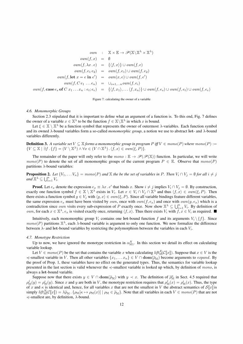
4.6. Monomorphic GroupsSection 2.3 stipulated that it is important to define what an argument of a function is. To this end, Fig. 7 defines

the owner of a variable x ∈ Xλ to be the function f ∈ X\Xλ in which x is bound.Let ξ ∈ X \ Xλ be a function symbol that represents the owner of outermost λ-variables. Each function symbol

and its owned λ-bound variables form a so-called monomorphic group, a notion we use to abstract let- and λ-boundvariables differently.

Definition 3. A variable set V ⊆ X forms a monomorphic group in program P iff V ∈ mono(P ) where mono(P ) :=V ⊆ X | ∃f . f = (V \ Xλ) ∧ ∀x ∈ (V ∩ Xλ) . 〈f, x〉 ∈ own(ξ, P ).

The remainder of the paper will only refer to the mono : E → P(P(X)) function. In particular, we will writemono(P ) to denote the set of all monomorphic groups of the current program P ∈ E. Observe that mono(P )partitions λ-bound variables:

Proposition 2. Let V1, . . . Vn = mono(P ) and X the be the set of variables in P . Then Vi ∩ Vj = ∅ for all i 6= jand Xλ ⊆

⋃ni=1 Vi.

Proof. Let ex denote the expression ex ≡ λx . e′ that binds x. Show i 6= j implies Vi ∩ Vj = ∅. By construction,exactly one function symbol f ∈ X \ Xλ exists in Vi. Let x ∈ Vi ∩ Vj ∩ Xλ and thus 〈f, x〉 ∈ own(ξ, P ). Thenthere exists a function symbol g ∈ Vj with 〈g, x〉 ∈ own(ξ, P ). Since all variable bindings feature different variables,the same expression ex must have been visited by own , once with own(f, ex) and once with own(g, ex) which is acontradiction since own visits every sub-expression of P exactly once. Now show Xλ ⊆

⋃ni=1 Vi. By definition of

own , for each x ∈ Xλ, ex is visited exactly once, returning 〈f, x〉. Thus there exists Vi with f, x ∈ Vi as required.

Intuitively, each monomorphic group Vi contains one let-bound function f and its arguments Vi \f. Sincemono(P ) partitions Xλ, each λ-bound variable is argument to only one function. We now formalize the differencebetween λ- and let-bound variables by restricting the polymorphism between the variables in each Vi.

4.7. Monotype RestrictionUp to now, we have ignored the monotype restriction in αXM1. In this section we detail its effect on calculating

variable lookup.Let V ∈ mono(P ) be the set that contains the variable x when calculating liftXM(C[[x]]). Suppose that x ∈ V is the

4-smallest variable in V . Then all other variables x1, . . . xn ∈ V ∩ dom(ρM) become arguments to expand . Bythe proof of Prop. 1, these variables have no effect on the generated types. Thus, the semantics for variable lookuppresented in the last section is valid whenever the 4-smallest variable is looked up which, by definition of mono, isalways a let-bound variable.

Suppose now that there exists y ∈ V ∩ dom(ρM) with y ≺ x. The definition of ρκM in Sect. 4.5 required thatρjM(y) = ρiM(y). Since x and y are both in V , the monotype restriction requires that ρjM(x) = ρiM(x). Thus, the typeof x and κ is identical and, hence, for all variables x that are not the smallest in V the abstract semantics of S[[x]] issimply liftXM(C[[x]]) = λρM . ρM[κ 7→ ρM(x)] | ρM ∈ ρM. Note that all variables in each V ∈ mono(P ) that are not4-smallest are, by definition, λ-bound.

12

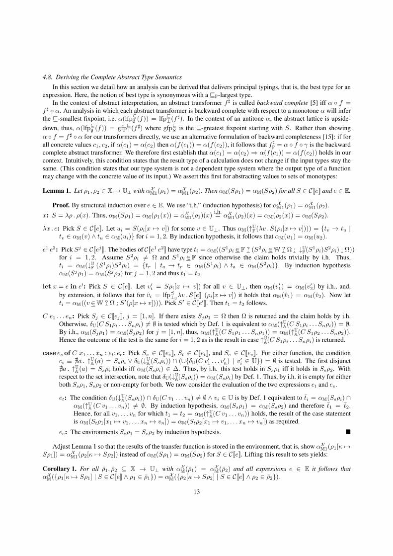
4.8. Deriving the Complete Abstract Type Semantics

In this section we detail how an analysis can be derived that delivers principal typings, that is, the best type for anexpression. Here, the notion of best type is synonymous with a vP-largest type.

In the context of abstract interpretation, an abstract transformer f ] is called backward complete [5] iff α f =f ] α. An analysis in which each abstract transformer is backward complete with respect to a monotone α will inferthe v-smallest fixpoint, i.e. α(lfp⊆∅ (f)) = lfpv⊥(f ]). In the context of an antitone α, the abstract lattice is upside-down, thus, α(lfp⊆∅ (f)) = gfpv>(f ]) where gfpvS is the v-greatest fixpoint starting with S. Rather than showingα f = f ] α for our transformers directly, we use an alternative formulation of backward completeness [15]: if forall concrete values c1, c2, if α(c1) = α(c2) then α(f(c1)) = α(f(c2)), it follows that f ]P = α f γ is the backwardcomplete abstract transformer. We therefore first establish that α(c1) = α(c2) ⇒ α(f(c1)) = α(f(c2)) holds in ourcontext. Intuitively, this condition states that the result type of a calculation does not change if the input types stay thesame. (This condition states that our type system is not a dependent type system where the output type of a functionmay change with the concrete value of its input.) We assert this first for abstracting values to sets of monotypes:

Lemma 1. Let ρ1, ρ2 ∈ X→ U⊥ with αXM1(ρ1) = αXM1(ρ2). Then αM(Sρ1) = αM(Sρ2) for all S ∈ C[[e]] and e ∈ E.

Proof. By structural induction over e ∈ E. We use “i.h.” (induction hypothesis) for αXM1(ρ1) = αXM1(ρ2).

x: S = λρ . ρ(x). Thus, αM(Sρ1) = αM(ρ1(x)) = αXM1(ρ1)(x)i.h.= αXM1(ρ2)(x) = αM(ρ2(x)) = αM(Sρ2).

λx . e: Pick S ∈ C[[e]]. Let ui = S(ρi[x 7→ v]) for some v ∈ U⊥. Thus αM(↑UF (λv . S(ρi[x 7→ v]))) = tv → tu |tv ∈ αM(v) ∧ tu ∈ αM(ui) for i = 1, 2. By induction hypothesis, it follows that αM(u1) = αM(u2).

e1 e2: Pick Sj ∈ C[[ej ]]. The bodies of C[[e1 e2]] have type ti = αM((S1ρi ∈F ? (S2ρi ∈W ? Ω : ↓UF(S1ρi)S2ρi) : Ω))

for i = 1, 2. Assume S2ρi 6= Ω and S1ρi ∈F since otherwise the claim holds trivially by i.h. Thus,ti = αM(↓UF (S1ρi)S

2ρi) = tr | ta → tr ∈ αM(S1ρi) ∧ ta ∈ αM(S2ρi). By induction hypothesisαM(Sjρ1) = αM(Sjρ2) for j = 1, 2 and thus t1 = t2.

let x = e in e′: Pick S ∈ C[[e]]. Let v′i = Sρi[x 7→ v]) for all v ∈ U⊥, then αM(v′1) = αM(v′2) by i.h., and,by extension, it follows that for vi = lfp⊥U

λv .S[[e]] (ρi[x 7→ v]) it holds that αM(v1) = αM(v2). Now letti = αM((v ∈W ? Ω : S′(ρ[x 7→ v]))). Pick S′ ∈ C[[e′]]. Then t1 = t2 follows.

C e1 . . . en: Pick Sj ∈ C[[ej ]], j = [1, n]. If there exists Sjρ1 = Ω then Ω is returned and the claim holds by i.h.Otherwise, δU(C S1ρi . . . Snρi) 6= ∅ is tested which by Def. 1 is equivalent to αM(↑UA(C S1ρi . . . Snρi)) = ∅.By i.h., αM(Sjρ1) = αM(Sjρ2) for j = [1, n], thus, αM(↑UA(C S1ρ1 . . . Snρ1)) = αM(↑UA(C S1ρ2 . . . Snρ2)).Hence the outcome of the test is the same for i = 1, 2 as is the result in case ↑UA(C S1ρi . . . Snρi) is returned.

case es of C x1 . . . xn : et; ee: Pick Ss ∈ C[[es]], St ∈ C[[et]], and Se ∈ C[[ee]]. For either function, the conditionci ≡ @a . ↑UA (a) = Ssρi ∨ δU(↓UA (Ssρi)) ∩ (∪δU(C v′1 . . . v

′n) | v′i ∈ U) = ∅ is tested. The first disjunct

@a . ↑UA(a) = Ssρi holds iff αM(Ssρi) ∈ ∆. Thus, by i.h. this test holds in Ssρ1 iff it holds in Ssρ2. Withrespect to the set intersection, note that δU(↓UA(Ssρi)) = αM(Ssρi) by Def. 1. Thus, by i.h. it is empty for eitherboth Ssρ1, Ssρ2 or non-empty for both. We now consider the evaluation of the two expressions et and ee.

et: The condition δU(↓UA(Ssρi)) ∩ δU(C v1 . . . vn) 6= ∅ ∧ vi ∈ U is by Def. 1 equivalent to ti = αM(Ssρi) ∩αM(↑UA (C v1 . . . vn)) 6= ∅. By induction hypothesis, αM(Ssρ1) = αM(Ssρ2) and therefore t1 = t2.Hence, for all v1, . . . vn for which t1 = t2 = αM(↑UA(C v1 . . . vn)) holds, the result of the case statementis αM(Stρ1[x1 7→ v1, . . . xn 7→ vn]) = αM(Stρ2[x1 7→ v1, . . . xn 7→ vn]) as required.

ee: The environments Seρ1 = Seρ2 by induction hypothesis.

Adjust Lemma 1 so that the results of the transfer function is stored in the environment, that is, show αXM1(ρ1[κ 7→Sρ1]) = αXM1(ρ2[κ 7→ Sρ2]) instead of αM(Sρ1) = αM(Sρ2) for S ∈ C[[e]]. Lifting this result to sets yields:

Corollary 1. For all ρ1, ρ2 ⊆ X → U⊥ with αXM(ρ1) = αXM(ρ2) and all expressions e ∈ E it follows thatαXM(ρ1[κ 7→ Sρ1] | S ∈ C[[e]] ∧ ρ1 ∈ ρ1) = αXM(ρ2[κ 7→ Sρ2] | S ∈ C[[e]] ∧ ρ2 ∈ ρ2).

13

By applying lca on each side of the equations we obtain Lemma 2:

Lemma 2. For all ρ1, ρ2 ⊆ X → U⊥ with lca(αXM(ρ1)) = lca(αXM(ρ2)) and all expressions e ∈ E, it follows thatlca(αXM(ρ1[κ 7→ Sρ1] | S ∈ C[[e]] ∧ ρ1 ∈ ρ1)) = lca(αXM(ρ2[κ 7→ Sρ2] | S ∈ C[[e]] ∧ ρ2 ∈ ρ2)).

Proof. For the sake of a contradiction, let ti = lca(αXM(ρi[κ 7→ Sρi] | S ∈ C[[e]] ∧ ρi ∈ ρi))κ and t1 6= t2.Then there exists S ∈ C[[e]] and ρiM ∈ P(X ∪ κ → M) such that ρiM ∈ αXM1(ρi[κ 7→ Sρi]) and ρ1

M(κ) 6= ρ2M(κ).

However, this is a contradiction to Lem. 1.

Lemma 2 allows us to derive backward complete abstract transfer functions as f ]P = α f γ for each concrete f .

4.9. Calculating the Best Abstract Transformers

In this section we derive abstract transformers for the semantic rules (aka concrete transformer) in Fig. 3. Theabstraction map liftXM in Fig. 6 takes a collecting semantics to a semantics over sets of type vectors and binds the resultto the special variable κ. Thus, the semantic equation over polymorphic types for an expression e ∈ E is given byT [[e]] := lca liftXM(C[[e]]) ground resulting in the polymorphic type (T [[e]]ρ)κ. Consider each rule in turn.

Variable. Equation (1) in Fig. 8 expands C[[x]] and pushes ground and lca into the set expression. Inlining the firstαXM1 results in Eq. (2) that returns type sets whose projection on X \ κ is bounded by ground(ρP) and αXM1(ρ).We chose ρ such that both bounds coincide which eliminates that intersection over all ρ. As discussed in Sect. 4.5,the monotype restriction in αXM1 creates the case distinction between let-bound variables and λ-bound variables. Theformer translates to an expand construct in Eq. (3) that Eq. (4) lifts to polytypes. Section 4.7 detailed that λ-boundvariables translate to a simple variable lookup, as implemented by Eq. (5).

Abstraction. Eqn. (6) expands liftXM before (7) pushes ground inside and moves lca past the intersection over ρ.Equation (8) expands the definition of C[[λx . e]] and Eqn. (9) expands the application of αM to the function type.Here, t1 → t2 replaces t. The lifting (10) follows from Lemma 1, rendering ρ unused, leading to Eqn. (11). Equation(12) follows by Lemma 2 with lca(M) = (a)≡P .

Application. We expand the standard semantics, giving Eqn. (13), and then inline αM in Eqn. (14). Observe that↑UF (↓UF (v1)) = v1 since v1 ∈ F. Now choose v2 for e which fixes ta, yielding Eqn. (15). Note here that no types aregenerated when ↓UF (v1)v2 is ⊥U. Equation (16) follows due to the identity αM γM, leading to the typing constraintin Eqn. (17). The latter translates to a meet expression gci, i.e., unification (18). Note here that the first case onlyapplies if unification succeeded, that is, if ρ′P 6= ⊥P.

Binding. After inlining liftXM in Fig. 9, the expanded semantic in Eqn. (19) is lifted to types in Eqn. (20) and the lfpis replaced with a greatest-fixpoint computation. Equation (21) lifts this fixpoint computation to one on polymorphictypes, thereby making the possibility that an empty environment is computed explicit by returning ⊥P.

Constructors. After pushing lca and ground inside, the collecting semantics C[[C e1 . . . en]] needs expanding inEqn. (22). We distinguish the case where Siρ∈W and the remaining if-statement in Fig. 3. With αM(Ω) = ∅, thetranslation of the first case yields Eqn. (23). The second case is represented by tc(ρP) and is computed in Eqn. (25).Mapping the constructor and its argument to a datatype is performed by δM and δP which are here defined as follows:

Definition 4. The datatype of a constructor is given by δP : C×P∗ → P⊥, namely: δP(Nil) = [(a)≡P ], δP(Cons h t) =gci([h], t) and δP(c) = Int for all c ∈ Z. Define δM : C×M∗ →P(P) as δM(C t1 . . . tn) = ground(δP(C t1 . . . tn)).

Thus, Eqn. (26) computes the datatype without resorting the concrete values. The lifting to polytypes in Eqn. (27)separates the empty set of types into an error case. This error case is merged with that of Eqn. (23), yielding Eqn. (24).

14

T[[·]

]:

E→

(X→

P)⊥ ≡

P→

(X∪κ→

P)⊥ ≡

P

T[[x

]]=

lcaλρM.⋂ α

X M1(ρ

[κ7→Sρ])|S∈C[

[x]]∧ρ∈γX M

(ρM

)gro

und

(1)

=λρP.lca

(⋂ ρ∈X→

U⊥αX M

1(ρ

[κ7→ρ(x

)])|g

round

(ρP)⊆αX M

1(ρ

))

(2)

=λρP.lca( ⋂ ρ

∈X→

U⊥

⋃ ρ

M⊆

X∪κ→

M∣ ∣ ∣ ∣∀ρ M

∈ρM,y∈X∪κ.ρM

(y)∈αM

(ρ[κ7→ρ(x

)](y

))∧

m.r.∧gro

und

(ρP)⊆∃ κ

(ρM

)⊆αX M

1(ρ

)

)ifx/∈Xλ

(3)

=λρP.lca

(∃y′ 1,...y′ n(expandxy1...y

n,κy′ 1...y′ n(gro

und

(ρP)

)w

herey

1,...y n

=y∈dom

(ρP)|x≺y

ifx/∈Xλ

(4)

=λρP.∃y′ 1,...y′ n(expandxy1...y

n,κy′ 1...y′ n(ρ

P))

whe

rey

1,...y n

=y∈dom

(ρP)|x≺y

ifx∈Xλ

(5)

=λρP.ρ

P[κ7→ρP(x

)]

T[[λx.e

]](6

)=

lcaλρM.(⋂ ρ∈X→

U⊥

(⋃ ρM

[κ7→t]|t∈αM

(Sρ)∧S∈C[

[λx.e

]]∧ρM∈ρM⊆αX M

1(ρ

)))gro

und

(7)

=λρP.⋂ ρ

∈X→

U⊥lcaρ

M[κ7→t]|t∈αM

(Sρ)∧S∈C[

[λx.e

]]∧ρM∈gro

und

(ρP)⊆αX M

1(ρ

)(8

)=

λρP.⋂ ρ

∈X→

U⊥lcaρ

M[κ7→t]|t∈αM

(↑U F(λv.S

(ρ[x7→v])

))∧S∈C[

[e]]∧ρM∈gro

und

(ρP)⊆αX M

1(ρ

)(9

)=

λρP.⋂ ρ

∈X→

U⊥lcaρ

M[κ7→t 1→t 2

]|v

2=S

(ρ[x7→v 1

])∧S∈C[

[e]]∧v 1∈U∧t i∈αM

(vi)∧ρM∈gro

und

(ρP)⊆αX M

1(ρ

)(1

0)

=λρP.⋂ ρ

∈X→

U⊥lcaρ

M[κ7→t 1→t 2

]|t

2=T

[[e]](ρM

[x7→t 1

])κ∧t 1∈M∧ρM∈gro

und

(ρP)⊆αX M

1(ρ

)(1

1)

=λρP.lcaρ

M[κ7→t 1→t 2

]|t

2=T

[[e]](ρM

[x7→t 1

])κ∧t 1∈M∧ρM∈gro

und

(ρP)

(12)

=λρP. ρ′ P[κ

7→t 1→t 2

]if⊥

P6=ρ′ P

=T

[[e]](ρP[x7→

(a) ≡

P])

andt 1

=ρ′ P(x

)an

dt 2

=ρ′ P(κ

)

⊥P

othe

rwis

eT

[[e1e 2

]]=

lcaλρM.(⋂ ρ∈X→

U⊥

(⋃ ρM

[κ7→t]|t∈αM

(Sρ)∧S∈C[

[e1e 2

]]∧ρM∈ρM⊆αX M

1(ρ

))gro

und

(13)

=λρP.lcaρ

M[κ7→t]|↓

U F(v

1)∈F∧v 26=

Ω∧t∈αM

(↓U F(v

1)v

2)∧env

whe

reenv≡v i

=Siρ∧Si∈S[

[ei]]∧ρM∈ρM⊆αX M

1(ρ

)(1

4)

=λρP.⋂ ρ

∈X→

U⊥lcaρ

M[κ7→t]|∃t a,tr∈M.↓U F

(v1)∈F∧v 26=

Ω∧↑U F

(↓U F(v

1))∈γM

(ta→t r

)∧∀v∈γM

(ta).↓U F

(v1)v∈γM

(tr)\⊥

P∧t∈αM

(↓U F(v

1)v

2)∧env

(15)

=λρP.⋂ ρ

∈X→

U⊥lcaρ

M[κ7→t]|∃t r∈M.v

1∈γM

(ta→t r

)∧v 2∈γM

(ta)∧↓U F

(v1)v

2∈γM

(tr)∧t∈αM

(↓U F(v

1)v

2)∧env

(16)

=λρP.⋂ ρ

∈X→

U⊥lcaρ

M[κ7→t r

]|∃t r∈M.v

1∈γM

(ta→t r

)∧v 2∈γM

(ta)∧env

(17)

=λρP. lc

aρ

M[κ7→t r

]|∃t r∈M.t

1=t a→t r∧t 2

=t a∧t i

=T

[[ei]]ρ

Mκ∧ρM∈gro

und

(ρP)

ifT

[[ei]]ρM6=∅

⊥P

othe

rwis

e(1

8)

=λρP. ρ′ P[κ

7→t r

]if⊥

P6=ρ′ P

=gci(T

[[e1]]ρ

P,ρP[κ7→

(T[[e

2]]ρ

Pκ)→

(a) ≡

P])

andT

[[ei]]ρP6=⊥

Pan

dle

tta→t r

=ρ′ P(κ

)

⊥P

othe

rwis

e

Figu

re8:

deriv

ing

the

type

infe

renc

eal

gori

thm

byab

stra

ctin

gth

eco

llect

ing

sem

antic

s,pa

rton

e

15

T[[letx

=eine′

]]=

lcaλρM.(⋂ ρ∈X→

U⊥

(⋃ ρM

[κ7→t]|t∈αM

(Sρ)∧S∈C[

[letx

=eine′

]]∧ρM∈ρM⊆αX M

1(ρ

)))gro

und

(19)

=λρP.⋂ ρ

∈X→

U⊥lcaρ

M[κ7→t′

]|v6=

Ω∧t′∈αM

(S′ ρ

[x7→v])∧S′∈S[

[e′ ]]∧v∈l

fp ⊥

Uλv.S

(ρ[x7→v])|S∈C[

[e]]∧

ρM∈gro

und

(ρP)⊆αX M

1(ρ

)(2

0)

=λρP.lcaρ

M[κ7→t′

]|t′∈T

[[e′ ]]

(ρM

[x7→t]

)κ∧t∈

gfp⊆ MλT.⋂ t∈

T(T

[[e]]ρ

M[x7→t]

)κ∧ρM∈gro

und

(ρP)

(21)

=λρP. T[[

e′]]ρ

P[x7→t]

if⊥

P6=t

=gfpv

P(a

) ≡Pλt.T

[[e]](ρP[x7→t]

)κ

⊥P

othe

rwis

eT

[[Ce 1...en]]

=lcaλρM.(⋂ ρ∈X→

U⊥

(⋃ ρM

[κ7→t]|t∈αM

(Sρ)∧S∈C[

[Ce 1...en]]∧ρM∈ρM⊆αX M

1(ρ

)))gro

und

(22)

=λρP.⋂ ρ

∈X→

U⊥lcaρ

M[κ7→t]|t∈αM

(Sρ)∧S∈C[

[Ce 1...en]]∧ρM∈gro

und

(ρP)⊆αX M

1(ρ

)(2

3)

=λρP. lc

a(∅

)(α

M(S

1ρ)

=∅∨...∨αM

(Snρ)

=∅)∧Si∈C[

[ei]]∧ρM∈gro

und

(ρP)⊆αX M

1(ρ

)t c

(ρP)

othe

rwis

e(2

4)

=λρP. ⊥ P

ifT

[[e1]]

=⊥

P∨...∨T

[[en]]

=⊥

P∨δ P

(C(T

[[e1]]ρ

P)...(T

[[en]]ρ

P))

=⊥

PρP[κ7→δ P

(C(T

[[e1]]ρ

P)...(T

[[en]]ρ

P))]

othe

rwis

e

whe

ret c

(25)

=λρP. lcaρ

M[κ7→t]|t∈αM

(δU(C

S1ρ...Snρ))∧Si∈C[

[ei]]∧ρM∈gro

und

(ρP)⊆αX M

1(ρ

)(2

6)

=λρP.lcaρ

M[κ7→t]|t∈δ M

(Ct 1...tn))∧t i∈αM

(Siρ

)∧Si∈C[

[ei]]∧ρM∈gro

und

(ρP)⊆αX M

1(ρ

)(2

7)

=λρP. ⊥ P

ifδ P

(C(T

[[e1]]ρ

P)...(T

[[en]]ρ

P))

=⊥

PρP[κ7→δ P

(C(T

[[e1]]ρ

P)...(T

[[en]]ρ

P))]

othe

rwis

eT

[[casee s

ofCx

1...xn

:e t

;ee]]

=lcaλρM.(⋂ ρ∈X→

U⊥

(⋃ ρM

[κ7→t]|t∈αM

(Sρ)∧S∈C[

[casee s

ofCx

1...xn

:e t

;ee]]∧ρM∈ρM⊆αX M

1(ρ

)))gro

und

=λρP.⋂ ρ

∈X→

U⊥lcaρ

M[κ7→t]|t∈αM

(Sρ)∧S∈C[

[casee s

ofCx

1...xn

:e t

;ee]]∧ρM∈gro

und

(ρP)⊆αX M

1(ρ

)

(28)

=λρP. lc

a(∅

)∀ρ∈X→

U⊥.@a.↑

U A(a

)=Ssρ∨δ U

(↓U A(Ssρ))∩

(∪δ

U(C

v′ 1...v′ n)|v′ i∈U)

=∅∧Ss∈C[

[es]]∧

ρM∈gro

und

(ρP)⊆αX M

1(ρ

)

gci(t t

(ρP),te(ρ

P))

othe

rwis

e(2

9)

=λρP. lca

(∅)

∀ρ∈X→

U⊥.α

M(Ssρ)∩

(∪δ

M(C

t′ 1...t′ n)|t′ i∈M)

=∅∧Ss∈C[

[es]]∧ρM∈gro

und

(ρP)⊆αX M

1(ρ

)

gci(t t

(ρP),te(ρ

P))

othe

rwis

e(3

0)

=λρP. ⊥ P

gci(T

[[es]]ρ

P,δ P

(C(a

) ≡P...(

a) ≡

P))

=⊥

Pgci(t t

(ρP),T

[[ee]]ρ

P)ot

herw

ise

whe

ret t

(31)

=λρP.⋂ ρ

∈X→

U⊥lcaρ

M[κ7→t]|t∈αM

(Sρ[x

17→v 1,...xn7→v n

])∧δ U

(↓U A(Ssρ))∩δ U

(Cv 1...vn)6=∅∧v i∈U∧

St∈C[

[et]]∧ρM∈gro

und

(ρP)⊆αX M

1(ρ

)(3

2)

=λρP.⋂ ρ

∈X→

U⊥lcaρ

M[κ7→t]|t∈αM

(Sρ[x

17→v 1,...xn7→v n

])∧αM

(Ssρ)∩δ M

(Ct 1...tn)6=∅∧v i∈U∧t i∈γM

(vi)∧

St∈C[

[et]]∧ρM∈gro

und

(ρP)⊆αX M

1(ρ

)(3

3)

=λρP.T

[[et]](∃ κ

(gci(ρ′ P[κ7→T

[[es]]ρ

P],ρ′ P[κ7→δ P

(Ct 1...tn)]

)))

whe

reρ′ P

=ρP[x

17→t 1,...xn7→t n

]an

dt 1

=(a

) ≡P,...t n

=(a

) ≡P

Figu

re9:

deriv

ing

the

type

infe

renc

eal

gori

thm

byab

stra

ctin

gth

eco

llect

ing

sem

antic

s,pa

rttw

o

16

x ∈ Xλ

ρP ` x : ρP(x)(VAR-LAM)

x ∈ X \ Xλ x, y1, . . . yn = mono(P )

ρP ` x : (expandxy1...yn,κy′1...y′n(ρP))(κ)(VAR)

ρP[x 7→ t1] ` e : t2 t1 freshρP ` λx . e : t1 → t2

(ABS)

ρP ` e1 : t1 ρP ` e2 : t2σ = mgu(t2 → tr, t1) tr fresh

σρP ` e1 e2 : σtr(APP)

ρP[x 7→ t] ` e : t t vP (a)≡P greatestρP[x 7→ t] ` e′ : t′

ρP ` let x = e in e′ : t′(LET)

Figure 10: inference rules deduced from the semantic equations

Conditional. We distinguish the common error case when expanding the semantics in Eqn. (28). The error conditionis lifted to monotypes in Eqn. (29) and to polytypes in Eqn. (30). The non-error cases translate to gci(tt(ρP), te(ρP))since both function sets in Fig. 3 can be executed. The latter trivially reduces to T [[ee]]ρP as shown in Eqn. (30). Thenon-trival case is developed in Eqn. (31). The test δU(↓UA(Ssρ)) ∩ δU(C v1 . . . vn) 6= ∅ over values is lifted to sets oftypes, yielding Eqn. (32). Since the values v1, . . . vn that pass this test are bound to x1, . . . xn, this relation needs to bemade explicit in the lifting to polytypes. To this end, Eqn. (33) binds the ti to a different type variable each and addsbindings to xi, yielding ρ′P. In order to cater for the test, we bind the type of es to the temporary variable κ in ρ′P andunify this environment with one where κ is bound to the datatype that C t1 . . . tn may belong to, thereby restrictingthe ti. The temporary variable κ is then removed using ∃κ before the environment is used to evaluate et.

4.10. Translation from Equations to Inference Rules

In order to illustrate the difference between the inference algorithm in Figs. 8, 9 and typing rules, we translatethem by writing each rule λρP . body(ρP) if cond as an inference rule with cond as antecedent and ρP ` body(ρP)κas consequence. A first concession is to drop all handling of type errors ⊥P. While the first three rules translatestraightforwardly, the application rule e1 e2 uses gci which can be simplified: Since both arguments share ρP, nosubstitutions will be calculated for them. Hence, it suffices to calculate the mgu for the κ-bound type and applythe substitution to the whole environment, the latter being indicated by writing σρP in the consequence. Finally,the calculation of the greatest fixpoint is colloquially stated by requiring that t is the vP-greatest solution for whichρP[x 7→ t] ` e : t holds. Overall, while the resulting typing rules are equivalent to the inference algorithm in Figs. 8and 9 (except for error checking), it is hard to see that they present an algorithm with a straightforward implementation.

5. Inference of Vector Sizes

In this section, we sketch how we augmented the type inference with bit vectors that are polymorphic in theirlength. To this end, let S = P(

∑i cixi = c | ci, c ∈ Z, xi ∈ X) be the universe of size constraint systems. The

solution of s ∈ S is given by γS : S → P(Z|X|) with γS(s) = 〈v1, . . . v|X|〉 ∈ Z|X| | s[x1/v1, . . . x|X|/v|X|] holds.For each s ∈ S let s≡S denote some normalized constraint system in row-echelon form with γS(s) = γS(s≡S). LetS≡S = s ∈ S | s≡S = s denote the set of normalized size constraint systems. Define the meet s1uSs2 = (s1∪s2)≡S

and s1 vS s2 iff γS(s1) ⊆ γS(s2). Then 〈S≡S ,vS,uS〉 is a complete semi-lattice.

5.1. Interaction between Type- and Size Domain

We extend the Herbrand abstractions that represent types with |a| ∈ P, the type of bit vectors of size a ∈ V,and also allow Herbrand constants N ⊃ P that may instantiate type variables representing bit-vector sizes. The typeinference now operates on tuples ρP B s ∈ P((X → P)≡P × S≡S)

⊥. The two domains are co-fibered [20], that is, adomain operation on the master domain ρP can invoke one or more domain operations on the slave domain s. Thereare three ways how the size domain is manipulated:

• During instantiation of a let-bound variable x from t to a new instance t′, we compute the substitutions[a1/b1, . . . an/bn] = mgu(t, t′) and update the size domain s to expanda1...an,b1...bn

(s).

17

• During the calculation of the meet ρ1P B s1 t ρ2

P B s2, we first calculate ρ′P = gci(ρ1P, ρ

2P). All resulting

substitutions of the form a/b or a/c where c ∈ N are also applied to s′ = s1 uS s2. Any equation of the forma = b or a = c, c ∈ N in s′ is applied as substitution [a/b], respectively [a/c], to ρ′P. The result is bottom ifeither domain is bottom.

• At the end of the let- and λ-rule, type variables may exist in s that no longer exist in ρP. Remove these variablesfrom s using Gaussian elimination.

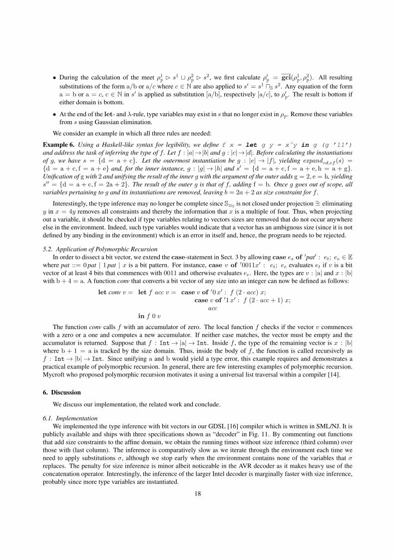
We consider an example in which all three rules are needed:

Example 6. Using a Haskell-like syntax for legibility, we define f x = let g y = xˆy in g (g ’11’)and address the task of inferring the type of f . Let f : |a|→|b| and g : |c|→|d|. Before calculating the instantiationsof g, we have s = d = a + c. Let the outermost instantiation be g : |e| → |f |, yielding expandcd,ef (s) =d = a + c, f = a + e and, for the inner instance, g : |g| → |h| and s′ = d = a + c, f = a + e,h = a + g.Unification of g with 2 and unifying the result of the inner g with the argument of the outer adds g = 2, e = h, yieldings′′ = d = a + c, f = 2a + 2. The result of the outer g is that of f , adding f = b. Once g goes out of scope, allvariables pertaining to g and its instantiations are removed, leaving b = 2a+ 2 as size constraint for f .

Interestingly, the type inference may no longer be complete since S≡S is not closed under projection ∃: eliminatingy in x = 4y removes all constraints and thereby the information that x is a multiple of four. Thus, when projectingout a variable, it should be checked if type variables relating to vectors sizes are removed that do not occur anywhereelse in the environment. Indeed, such type variables would indicate that a vector has an ambiguous size (since it is notdefined by any binding in the environment) which is an error in itself and, hence, the program needs to be rejected.

5.2. Application of Polymorphic RecursionIn order to dissect a bit vector, we extend the case-statement in Sect. 3 by allowing case es of

′pat′ : et; ee ∈ Ewhere pat ::= 0 pat | 1 pat | x is a bit pattern. For instance, case v of ′0011x′ : et; ee evaluates et if v is a bitvector of at least 4 bits that commences with 0011 and otherwise evaluates ee. Here, the types are v : |a| and x : |b|with b + 4 = a. A function conv that converts a bit vector of any size into an integer can now be defined as follows:

let conv v = let f acc v = case v of ′0x′ : f (2 · acc) x;case v of ′1x′ : f (2 · acc + 1) x;

accin f 0 v

The function conv calls f with an accumulator of zero. The local function f checks if the vector v commenceswith a zero or a one and computes a new accumulator. If neither case matches, the vector must be empty and theaccumulator is returned. Suppose that f : Int→ |a| → Int. Inside f , the type of the remaining vector is x : |b|where b + 1 = a is tracked by the size domain. Thus, inside the body of f , the function is called recursively asf : Int→ |b| → Int. Since unifying a and b would yield a type error, this example requires and demonstrates apractical example of polymorphic recursion. In general, there are few interesting examples of polymorphic recursion.Mycroft who proposed polymorphic recursion motivates it using a universal list traversal within a compiler [14].

6. Discussion

We discuss our implementation, the related work and conclude.

6.1. ImplementationWe implemented the type inference with bit vectors in our GDSL [16] compiler which is written in SML/NJ. It is

publicly available and ships with three specifications shown as “decoder” in Fig. 11. By commenting out functionsthat add size constraints to the affine domain, we obtain the running times without size inference (third column) overthose with (last column). The inference is comparatively slow as we iterate through the environment each time weneed to apply substitutions σ, although we stop early when the environment contains none of the variables that σreplaces. The penalty for size inference is minor albeit noticeable in the AVR decoder as it makes heavy use of theconcatenation operator. Interestingly, the inference of the larger Intel decoder is marginally faster with size inference,probably since more type variables are instantiated.

18

decoder lines time w/o sizes time w. sizesTexas MSP430 217 0.1s 0.2sAtmel AVR 941 1.6s 1.9sIntel x86 5610 3.7s 3.6s

Figure 11: performance of type checking various decoders

6.2. Observing Non-Termination through an Extended Occurs CheckThe lattice of Herbrand abstractions has infinite descending chains [11], that is, during a fixpoint computation the

type of a function may arbitrarily often be instantiated, thereby creating at least as many type variables than unificationeliminates. Thus, the fixpoint computation may not terminate. The possibility of non-termination follows from theundecidability of inferring a polymorphic recursive type for a function [8]. However, all non-terminating programs weknow are type incorrect. As an example, consider the function f x = f (x 1). Suppose we compute a fixpointfor f starting with f : a→b, thus x : a. When evaluating the body of the function, we instantiate f to f : c→d andobserve that x : Int→c thereby applying the substitution a/Int→c. In the next iteration, we have f : (Int→c)→b.Checking the body creates another instance f : (Int→ e)→ g and we observe that x : Int→ (Int→ e), therebyapplying the substitution c/(Int → e). Now the function type is f : (Int → (Int → e)) → b. We can checkfor these re-occurring patterns before each fixpoint iteration by simply unifying the uninstantiated type of f witheach of its usage sites. For instance, the unification of the current type of f with the current type of its usage givesgci((Int → (Int → e)) → b, (Int → e) → g) = ⊥P. In particular, the unification fails since the substitutione/Int→e triggers an occurs check. In this case, we abort the fixpoint computation since the refinement of f will goon indefinitely. If the unification succeeds then the function is not polymorphic recursive, that is, unifying the functionwith all its call sites is exactly what Damas’W algorithm does. Thus, if the unification fails for other reasons (that is,due to a constructor clash), we ignore this and continue with the fixpoint computation to find a polymorphic recursivetype. Although this extended occurs check is very simple, it catches all non-terminating behaviors we have observedso far, thereby giving a practical inference for polymorphic recursive types.

6.3. Related WorkTofte [19] observes the following about devising new type systems:

Guessing and verifying are inseparable parts of developing a new theory. None is prior to the other neitherin time nor in importance. I believe the reason why the guessing has been so hard is precisely that theverifying has been hard.

Instead of guessing, Cousot [1] proposes to use his abstract interpretation framework [2] to systematically con-struct type inferences (and thus type systems) by abstracting the language semantics, thereby replacing the hard taskof verification. We build on this work. However, Cousot partitions type variables into those bound in a type schemeand those that are free which, as shown by Ex. 2, is not generally possible. Moreover, his derived inference for Milner-Mycroft types [14] eliminates and re-introduces type schemes in every rule which instantiates λ-bound variables justlike let-bound variables, leading to types that are too general.

Type schemes seem to be a brittle, since syntactic, concept. Henglein’s inference for polymorphic recursion [8]gathers type variables of certain λ-bound variables in order to prevent them from being generalized. However, hisalgorithm collects the wrong variables [4, p. 164]. In fact, Henglein’s reduction from semi-unification to polymorphicrecursion is complicated by the incorrect inference and a corrected reduction should be much simpler.

The use of expansion [17] instead of type schemes can avoid the complex proofs involving arguments about freeand bound type variables [4, 12] and immediately lends itself to new applications as in the instantiation of vector sizeinformation as discussed in Sect. 5. Other results in the abstract interpretation literature, namely on completeness[2, 5, 15] and modularity [6], deserve highlighting in the context of type systems: By specifying a type inference of alanguage by the universe of types and requiring a modular and complete type inference, there is neither ambiguity ofwhat types must be inferable nor a prescription of the employed algorithm. However, given that the lattice of Herbrandabstractions 〈P,vP〉 has infinite descending chains, the only work on using abstract interpretation for type inferenceproposes to apply widening to ensure termination of the fixpoint computation [1, 7] rather than addressing the bigger

19

challenge [5] of restricting the lattice to avoid infinite descending chains. Even then, neither Gori and Levi [7] nor Jim[9] found any type correct program that required many iterations to type check which coincides with our experience.In particular, only incorrect programs in which instantiation replaces a type variable a by an expression involving aseem to trigger an infinite refinement. Since these trivial cases are found by our extended occurs check, we are asof yet not aware of any program for which our inference does not terminate. Thus, it might be worth ignoring theproblem of infinite descending chains and to further investigate into complete extensions such as our size inference.

Since Wells states that the Hindley-Milner type system has no “principal typings” [21], the chasm to our workneeds to be explained: Wells’ notion demands three properties of a type system to have principal typings: translatedto abstract interpretation nomenclature, these are completeness of transfer functions, condensing domains [6] (whichare both fair) and that types must be inferable in a bottom-up manner (which is unfair to Hindley-Milner since let-and λ-bound variables are abstracted differently and in a bottom-up analysis where variables are encountered beforetheir definition sites). In fact, the existence of αXM in Fig. 6 alone guarantees that a best type exists, although it mightnot be possible to infer it. Note that Cousot only defined γXM explicitly and defined αXM in terms of γXM [1], whichseems to suggest that defining an αXM as we have done in this work is non-trival.

6.4. ConclusionWe derived a type inference algorithm for the Hindley-Milner type system using the abstract interpretation frame-

work. In contrast to previous work, our derived algorithm is complete by construction by being built on a novelαXM featuring a monotype restriction. We proposed expansion over type schemes to handle instantiation. The latterallowed us to construct a complete inference for vector sizes.

Acknowledgements. I thank Jan Midtgaard and the anonymous reviewers for improving the presentation and RobertoGiacobazzi and Andy King for useful discussions.

[1] P. Cousot. Types as Abstract Interpretations. In Principles of Programming Languages, pages 316–331, Paris, France, January 1997. ACM.invited paper.

[2] P. Cousot and R. Cousot. Systematic Design of Program Analysis Frameworks. In Principles of Programming Languages, pages 269–282,San Antonio, Texas, USA, January 1979. ACM.

[3] L. Damas and R. Milner. Principal Type-Schemes for Functional Programs. In Principles of Programming Languages, pages 207–212,Albuquerque, New Mexico, USA, 1982. ACM.

[4] M. Emms and H. Leiß. Extending the type checker of Standard ML by polymorphic recursion. Theoretical Computer Science, 212(1-2):157– 181, 1999.

[5] R. Giacobazzi, F. Ranzato, and F. Scozzari. Making abstract interpretations complete. Journal of the ACM, 47(2):361–416, 2000.[6] R. Giacobazzi, F. Ranzato, and F. Scozzari. Making abstract domains condensing. Trans. Comput. Log., 6(1):33–60, 2005.[7] R. Gori and G. Levi. An Experiment in Type Inference and Verification by Abstract Interpretation. In A. Cortesi, editor, Verification, Model

Checking, and Abstract Interpretation, volume 2294 of LNCS, pages 237–241, Venice, Italy, January 2002. Springer.[8] F. Henglein. Type Inference with Polymorphic Recursion. Transactions on Programming Languages and Systems, 15:253–289, 1991.[9] Trevor Jim. What are principal typings and what are they good for? In Principles of Programming Languages, pages 42–53, St. Petersburg

Beach, Florida, USA, 1996. ACM.[10] M. Karr. On affine relationships among variables of a program. Acta Informatica, 6(2):133–151, 1976.[11] J.-L. Lassez, M. J. Maher, and K. Marriott. Unification Revisited. In M. Boscarol, L. Carlucci Aiello, and G. Levi, editors, Foundations of

Logic and Functional Programming, volume 306 of LNCS, pages 67–113, Trento, Italy, December 1986. Springer.[12] S. Lenglet and J. Wells. Expansion for Universal Quantifiers. In H. Seidl, editor, European Symp. on Prog. Lang. and Systems, volume 7211

of LNCS, pages 456–475, Tallinn, Estonia, March 2012. Springer.[13] R. Milner. A Theory of Type Polymorphism in Programming. J. Comput. Sys. Sci., 17(3):348–375, 1978.[14] A. Mycroft. Polymorphic Type Schemes and Recursive Definitions. In M. Paul and B. Robinet, editors, Symposium on Programming, volume

167 of LNCS, pages 217–228, Toulouse, France, April 1984. Springer.[15] D. A. Schmidt. Comparing Completeness Properties of Static Analyses and Their Logics. In N. Kobayashi, editor, Asian Symposium on

Programming Languages and Systems, volume 4279 of LNCS, pages 183–199, Sydney, Australia, November 2006. Springer.[16] A. Sepp, J. Kranz, and A. Simon. GDSL: A Generic Decoder Specification Language for Interpreting Machine Language. In Tools for

Automatic Program Analysis, ENTCS, Deauville, France, September 2012. Springer.[17] H. Siegel and A. Simon. Summarized Dimensions Revisited. In L. Mauborgne, editor, Workshop on Numeric and Symbolic Abstract Domains,

ENTCS, Venice, Italy, September 2011. Springer.[18] A. Simon. Deriving a Complete Type Inference for Hindley-Milner and Vector Sizes using Expansion. In Partial Evaluation and Program

Manipulation, SIGPLAN, Rome, Italy, January 2013. ACM.[19] M. Tofte. Operational Semantics and Polymorphic Type Inference. PhD thesis, University of Edinburgh, UK, 1988.[20] A. Venet. Abstract Cofibered Domains: Application to the Alias Analysis of Untyped Programs. In Static Analysis Symposium, LNCS, pages

366–382, London, UK, 1996. Springer.[21] J. B. Wells. The Essence of Principal Typings. In P. Widmayer, F. T. Ruiz, R. M. Bueno, M. Hennessy, S. Eidenbenz, and R. Conejo, editors,

Colloquium on Automata, Languages and Programming, volume 2380 of LNCS, pages 913–925, Malaga, Spain, July 2002. Springer.

20