description of fault detection and identification ...sail.unist.ac.kr/papers/prodiag_2014.pdf ·...
TRANSCRIPT

ANL/NE-12/57
Description of Fault Detection and Identification
Algorithms for Sensor and Equipment Failures and
Preliminary Tests Using Simulations
Nuclear Engineering Division


About Argonne National Laboratory Argonne is a U.S. Department of Energy laboratory managed by UChicago Argonne, LLC under contract DE-AC02-06CH11357. The Laboratory’s main facility is outside Chicago, at 9700 South Cass Avenue, Argonne, Illinois 60439. For information about Argonne and its pioneering science and technology programs, see www.anl.gov.
Availability of This Report This report is available, at no cost, at http://www.osti.gov/bridge. It is also available on paper to the U.S. Department of Energy and its contractors, for a processing fee, from:
U.S. Department of Energy
Office of Scientific and Technical Information
P.O. Box 62
Oak Ridge, TN 37831-0062
phone (865) 576-8401
fax (865) 576-5728
Disclaimer This report was prepared as an account of work sponsored by an agency of the United States Government. Neither the United States Government nor any agency thereof, nor UChicago Argonne, LLC, nor any of their employees or officers, makes any warranty, express or implied, or assumes any legal liability or responsibility for the accuracy, completeness, or usefulness of any information, apparatus,
product, or process disclosed, or represents that its use would not infringe privately owned rights. Reference herein to any specific commercial product, process, or service by trade name, trademark, manufacturer, or otherwise, does not necessarily constitute or imply its endorsement, recommendation, or favoring by the United States Government or any agency thereof. The views and opinions of
document authors expressed herein do not necessarily state or reflect those of the United States Government or any agency thereof, Argonne National Laboratory, or UChicago Argonne, LLC.
ANL/NE-12/57
Description of Fault Detection and Identification Algorithms for
Sensor and Equipment Failures and Preliminary Tests Using
Simulations
prepared by R.B. Vilim, A. Heifetz, Y.S. Park, and J. Choi Nuclear Engineering Division, Argonne National Laboratory November 30, 2012

Description of Fault Detection and Identification Algorithms for Sensor and Equipment Failures and
Preliminary Tests Using Simulations
November 30, 2012
ANL/NE-12/57 iii
Page intentionally blank

Description of Fault Detection and Identification Algorithms for Sensor and Equipment Failures and
Preliminary Tests Using Simulations iv November 30, 2012
ABSTRACT
On-going research to develop and evaluate operator aids that can facilitate more timely response to plant faults and grid disturbances and thereby increase plant resilience is described. The work involves collaboration between Argonne National Laboratory (ANL) and Idaho National Laboratory (INL). This research examines how technology advances can contribute to increased operator awareness and aid in better formulating a response to upsets. Control actions executed in a timely manner before the plant state reaches safety settings can increase plant resilience. Ready access to procedures and to planning tools that provide trends and can project ahead based on proposed control actions support this goal. Advanced automation can play a role. There is a lag in the speed with which human operators can progress through a procedure - observing all the “procedure adherence” expectations to avoid human error. Automation can take the plant to an acceptable state more quickly. Work on three elements that address these objectives is described. A new method and approach for detecting sensor degradation and substitution of the degraded sensor reading with a high-quality estimate for the value of the underlying process variable is described. A method for diagnosing from instrumented process variables the identity of an equipment failure is described. These two capabilities provide assurance that the plant condition is known providing an opportunity for application of a third element, more refined control through automation. A technology demonstration platform to aid in the visualization of how these technologies might integrate is described. It provides an environment for simulating the linkages among algorithms for sensor fault estimation, component fault diagnosis, and advanced control with the objective of better understanding the interactions among these three component technologies.
Description of Fault Detection and Identification Algorithms for Sensor and Equipment Failures and
Preliminary Tests Using Simulations
November 30, 2012
ANL/NE-12/57 v
Table of Contents
ABSTRACT ................................................................................................................................... iv
List of Figures ................................................................................................................................ vi
1 Introduction ................................................................................................................................ 1
1.1 Background ......................................................................................................................... 1 1.2 Technical Issue and Objective ............................................................................................ 2 1.3 Approach ............................................................................................................................. 3 1.4 Organization ........................................................................................................................ 5
2 Sensor Fault Estimation .............................................................................................................. 6
2.1 Background ........................................................................................................................... 6 2.2 State of the Art ...................................................................................................................... 6 2.3 Gap Analysis......................................................................................................................... 8 2.4 New Algorithm: AFTR-MSET ............................................................................................. 8 2.5 Models ................................................................................................................................ 10 2.5.1 Resistance Temperature Detector ......................................................................... 10 2.5.2 Printed Circuit Heat Exchanger ............................................................................ 15 2.6 Algorithm Results ............................................................................................................... 16 2.6.1 MSET – Application to Monitoring Dynamic Sensor Response .......................... 16 2.6.2 AFTR-MSET ........................................................................................................ 20
3 Component Fault Identification ................................................................................................ 26
3.1 Background ....................................................................................................................... 26 3.2 Algorithms ........................................................................................................................ 27 3.3 Results. .............................................................................................................................. 29
4 Automation for Fault Recovery ................................................................................................ 35
4.1 Background ....................................................................................................................... 35 4.2 Advanced Control Technologies ....................................................................................... 35 4.3 Collaboration ..................................................................................................................... 36 4.4 Automation to Replace Procedure-Based Manual Control ............................................... 36
5 Technology Demonstration Platform ....................................................................................... 37
5.1 Architecture ....................................................................................................................... 37 5.2 Modules ............................................................................................................................. 42 5.2.1 Plant ...................................................................................................................... 42 5.2.2 Control and Protection Systems ............................................................................ 43 5.2.3 Signal Processing Routines ................................................................................... 46 5.3 Operator Station ................................................................................................................ 47
6 Future Work .............................................................................................................................. 48
7 Conclusion ................................................................................................................................ 50
8 References ................................................................................................................................ 51
Description of Fault Detection and Identification Algorithms for Sensor and Equipment Failures and
Preliminary Tests Using Simulations vi November 30, 2012 LIST OF FIGURES
Figure 1.1 Current Paper-Based Manual Procedures for Recovery from an Internal Fault ...... 1
Figure 1.2 Envisioned Computer-Based Procedures and Operator Aids for Enhanced Fault Recovery ......................................................................................................... 5
Figure 2.1 Resistance Temperature Detector .......................................................................... 10
Figure 2.2 Schematics of Dynamical System Model of RTD Performance ........................... 11
Figure 2.3 Dynamics of Two Correlated Sensors .................................................................. 14
Figure 2.4. Schematic Drawing of Sensor Fault Detection in Four Sensors Connected to Input and Output of PCHE .................................................................................... 15
Figure 2.5 Different Training and Monitoring Transients Connecting the Same Initial and Final Steady-State RTD State Vectors .................................................................. 17
Figure 2.6. Parametric Plots (x vs. u) Graphical Representation of the RTD response. .......... 17
Figure 2.7 Estimation of RTD Input and Output Temperatures of the Monitoring Transient with MSET BART Kernel Trained on the RTD Training Transient..... 18
Figure 2.8 Parametric Plot of RTD States in the Memory Matrix Populated with Vectors of the Training Transient ....................................................................................... 19
Figure 2.9 MSET BART Kernel Estimation of Monitoring Transient Using Memory Matrix Populated with Vectors of the Training Transient ..................................... 19
Figure 2.10 Schematic Diagram of Two Correlated RTD’s Driven by the Same Forcing Function ................................................................................................................. 20
Figure 2.11 Training and Monitoring Transients for Fault Detection in a System of Two Correlated RTD’s .................................................................................................. 21
Figure 2.12 Estimation of Two RTD’s with L2 Norm and Vectors Learned from the Training Data ......................................................................................................... 21
Figure 2.13 Estimation of Two RTD’s with Proprietary Norm Minimization and Vectors Learned from Training Data .................................................................................. 22
Figure 2.14 Schematic Diagram of HTR Dynamics with HOT and COLD Inputs and
Outputs................................................................................................................... 22
Figure 2.15 Training and Monitoring Transients for One Input and Two Outputs (HOT and COLD) of HTR … .......................................................................................... 23
Figure 2.16 Fault Detection and Attribution with the Vectors Learned from the Training Data and Proprietary Norm Minimization ............................................................. 24
Figure 2.17 Training and Monitoring Transients for the Input and Outputs (HOT and COLD) of HTR for the Case when Both HTR inputs are Changing. .................... 25
Figure 2.18 Fault Detection and Attribution with the Vectors Learned from the Training Data and Proprietary Norm Minimization ............................................................. 25

Description of Fault Detection and Identification Algorithms for Sensor and Equipment Failures and
Preliminary Tests Using Simulations
November 30, 2012
ANL/NE-12/57 vii
Figure 3.1 Fault Diagnosis GUI Showing Clogged Filter in CVCS as Identified by PRODIAG ............................................................................................................. 27
Figure 3.2 Mapping of Sensor Signals into Faulty Components through the Three Knowledge Bases of PRODIAG ........................................................................... 29
Figure 3.3 Execution Flow and Logic in PRODIAG as Determined by Manual Inspection of the Coding ......................................................................................................... 30
Figure 3.4 Comparison of Diagnoses Based on Forward-Chaining and Backward-Chaining Rule Evaluation ...................................................................................... 31
Figure 3.5 Example of a Plant Component (Single-Phase Heat Exchanger) Represented in JBoss Drool in Object-Oriented Format ............................................................ 33
Figure 3.6 Example of a Confluence Rule for a Plant Component (Single-Phase Heat Exchanger) as Represented in JBoss Drool in Object-Oriented Format ............... 34
Figure 5.1 EPICS Organization .............................................................................................. 38
Figure 5.2 Examples of EPICS Records ................................................................................. 39
Figure 5.3 Structure of IOC .................................................................................................... 39
Figure 5.4 EPICS Structure for Interfacing GUIs with Databases ......................................... 40
Figure 5.5 Python Bridge Program and Its Relation to Databases and Plant Models ............. 41
Figure 5.6 Schematic of Computer System Interfaces ............................................................ 41
Figure 5.7 Time Sequencing and Handshaking of Tasks in Plant Simulator ......................... 42
Figure 5.8 Schematic of a Propotional-Intergral-Derivative Controller ................................. 44
Figure 5.9 SCM Block Diagram of a PI Controller ................................................................ 44
Figure 5.10 Representation of the SCM Generator Power Controller. Wiith Bpass, Inventory, and Mixed Controller ........................................................................... 46
Figure 5.11 Block Diagram of Precooler Temperature PI Controller ....................................... 46
Figure 5.12 Signal Processing Algorithm Execution under EPICS .......................................... 47
Figure 5.13 Plant Control Station Window ............................................................................... 48
Figure 5.14 Real Time Status Station Window ......................................................................... 49

Description of Fault Detection and Identification Algorithms for Sensor and Equipment Failures and
Preliminary Tests Using Simulations viii November 30, 2012
Page intentionally blank
Description of Fault Detection and Identification Algorithms for Sensor and Equipment Failures and
Preliminary Tests Using Simulations
November 30, 2012
ANL/NE-12/57 ix
ACRONYMS
ANL Argonne National Laboratory ARC Advanced Reactor Concepts ARMA Auto Regressive Moving Average ASI Advanced Sensors and Instrumentation CCD Classification Dictionary CVCS Chemical and Volume Control System CCW Component Cooling Water System DOE Department of Energy GPASS General Plant Analyzer and System Simulator HTR High Temperature Recuperator IDE Integrated Development Environment INL Idaho National Laboratory LS Least Squares LWRS Light Water Reactor Sustainability MSET Multivariate State Estimation Technique NE Nuclear Energy NEET Nuclear Energy Enabling Technologies NPP Nuclear Power Plant NRC Nuclear Regulatory Commission PID Piping Database PIDB Piping and Instrumentation Database PRD Physical Rules Database PID Proportional Integral Derivative PCHE Printed Circuit Heat Exchanger PCS Plant Control System PRE Precoller PWR Pressurized Water Reactor RTD Resistance Temperature Detector SMR Small Modular Reactor SVD Singular Value Decomposition TH Thermal Hydraulic

Description of Fault Detection and Identification Algorithms for Sensor and Equipment Failures and
Preliminary Tests Using Simulations
November 30, 2012
ANL/NE-12/57 1
1. Introduction
The Advanced Sensors and Instrumentation (ASI) technology area under the Nuclear Energy Enabling Technologies (NEET) Program was created by the U.S. Department of Energy (DOE) Office of Nuclear Energy (NE) to coordinate instrumentation and controls (I&C) research across DOE-NE programs and to identify and address common needs. The project Design to Achieve Fault Tolerance and Resilience, one of ten projects in the NEET ASI technology-area portfolio, is the subject of this report. This project is to develop and evaluate operator aids that can facilitate more timely response to plant faults and grid disturbances and thereby increase plant resilience for such events. The project involves collaboration between Argonne National Laboratory (ANL) and Idaho National Laboratory (INL). It leverages many tens of man-years of ANL experience in the development of equipment fault detection and identification algorithms and the design of control and protection systems for advanced reactors with a comparable amount of experience at INL in the design, licensing, operating, and maintaining of existing and advanced light water reactors.
1.1 Background
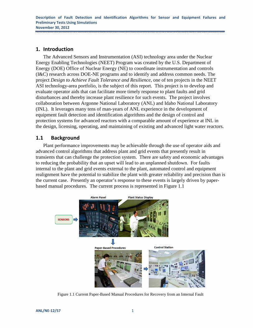
Plant performance improvements may be achievable through the use of operator aids and advanced control algorithms that address plant and grid events that presently result in transients that can challenge the protection system. There are safety and economic advantages to reducing the probability that an upset will lead to an unplanned shutdown. For faults internal to the plant and grid events external to the plant, automated control and equipment realignment have the potential to stabilize the plant with greater reliability and precision than is the current case. Presently an operator’s response to these events is largely driven by paper-based manual procedures. The current process is represented in Figure 1.1
Figure 1.1 Current Paper-Based Manual Procedures for Recovery from an Internal Fault

Description of Fault Detection and Identification Algorithms for Sensor and Equipment Failures and
Preliminary Tests Using Simulations 2 November 30, 2012
The control systems in today’s fleet of commercial nuclear power plants were designed
using the concept of hierarchical supervisory control. This mode of control assumes that electric demand does not change rapidly, typically limited to step changes of ten percent and ramp changes of three percent per minute. Plant systems essentially behave quasi-statically within the plant control system (PCS) envelope under these conditions. But for some plant duty-cycle events a significant imbalance in heat production and generation develops across the plant creating short term conditions that for the current design of the protection system results in a plant trip. As an example, many existing plants are not able to run back to house load after a full loss of load event, tripping instead on reactor protection system function.
Advanced algorithms might make use of anticipatory signals to better match primary heat rates with the balance-of-plant heat rate in combination with momentary excursion of trip settings to avoid tripping the plant. The use of feed-forward control might be used in combination with existing feedback loops to buffer the reactor from disturbances originating on the grid or in the balance of plant. As an example, the steam generator provides an energy storage capability that under current control algorithms is not fully exploited for its capability to buffer the plant from grid events. With re-engineered control algorithms it may be possible to disconnect from the grid on a rapid power runback. This allows for a quick reconnect rather than the precipitous shutdown and attendant equipment realignment that presently occurs after a trip.
The incentive to pursue advanced strategies for handling these events reflects what has
been learned of plant faults from the accumulated maintenance records of fifty years of operation. Computerized maintenance records of internal plant faults and their operational consequences provide insight for improving operation through more informed control and protection system design incorporating the updated condition status of the plant components. With the power of modern computing hardware and software now sufficient to provide the updated status of plant component condition, it may now be possible to better match control room tasks to the operator’s strengths and weaknesses. Automated systems perform more reliably than humans at rote tasks such as procedures-driven control actions. Humans on the other hand perform better at system oversight, evaluating complex situations and formulating an appropriate response. These new approaches benefit not only light water reactors but have applicability to the operation of advanced reactor concepts as well.
1.2 Technical Issue and Objective
A commercial nuclear power plant must operate safely, reliably, and with high efficiency and availability while meeting the production demands of a central power grid. These performance goals can, however, be challenged by events external to the plant (such as grid disturbances) or internal faults (such as component degradation, component failure, and operator error). Successful recovery from these events before they result in a protection system trip (and, hence, furthering the above goals) requires the operator to correctly identify the fault and to take the correct control action all in a timely manner. However, at present the operator is hampered by the need to first process a myriad of sensor data to identify the fault

Description of Fault Detection and Identification Algorithms for Sensor and Equipment Failures and
Preliminary Tests Using Simulations
November 30, 2012
ANL/NE-12/57 3
and then, assuming he has made a correct diagnosis, follow a paper-based set of procedures to recover from the fault. Both steps are time-consuming and their execution prone to error.
The objective of this multi-year project is to perform research that can lead to greater
resilience of nuclear power plants through the development and application of advanced technologies to improve operator awareness and decision making. Long term project goals include:
• Integration of fault detection and identification with automatic control algorithms for operation in a plant simulation environment.
• Installation of these integrated tools on a technology demonstration platform.
• Consideration of human factors in the design of the technology demonstration platform.
• Demonstration to the power-reactor industry of automated system response to detected and identified component degradation or failures to highlight the value compared to current manual procedures.
Objectives for FY12 as stated in the project research plan [1] and whose progress is reported on in this document are:
• Modernize and Extend Fault Detection and Identification Algorithms and Software - The principles that underlie the MSET and PRODIAG packages are still valid today but recent advances in software design tools leave their coding dated with respect to ease of maintenance and use. Work will begin to bring these tools up to a level where they can be easily interfaced with a modern event-based control-systems package.
• Develop Software Architecture for Simulator Platform for Demonstration of
Automated Control - The performance improvements sought under this project will be demonstrated on a simulation platform. The simulator will support execution of the fault detection and identification algorithms under concurrent plant simulation. It will be used to study plant response under automated control to perform the required equipment-realignment procedures.
1.3 Approach
A plant that can operate with greater flexibility and agility will be more resilient to the events described above. Resilience will be increased when degraded equipment is readily sensed. Advance notice of a failing component before alarm setpoints are reached provides an operator or an automatic control system greater time to act increasing the likelihood of averting a shutdown. Similarly for external events, if a plant is forced off the grid by a grid disturbance but is able to execute a controlled runback in power before protection system shutdown, then the plant is available for a quick reconnect. The plant is more resilient than

Description of Fault Detection and Identification Algorithms for Sensor and Equipment Failures and
Preliminary Tests Using Simulations 4 November 30, 2012 otherwise since grid demand can be met sooner and alternate electricity sources are not needed in the interim to meet house load.
The instrumentation and control system is a key element for achieving greater resilience to
faults. The enabler is digital system technology. With it the computationally intensive information processing associated with advanced real-time instrumentation and control algorithms is possible. Greater resilience can be realized in several ways.
• Reduced plant deviation through earlier detection and identification of failures.
• Tighter process variable regulation for improved plant trajectory management during upsets for avoidance of trip signals.
• Timelier operator response to events through the use of computer-prompted automated
procedures rather than paper-based manual procedures. All these capabilities can be realized through the design of the instrumentation and control system without negatively impacting the steady-state performance of the plant. In fact they may actually open up the design space in that the designer can take advantage of the resulting reduced likelihood and consequence of events that adversely affect safety, reliably, and availability.
In this work technology advances are examined that potentially can contribute to improved operator awareness and decision making for more agile plant operation and thus greater resilience to stressors.
Improved operator awareness of the plant state contributes to resiliency. At a most basic
level operator awareness is acquired from sensor readings. However, awareness can be improved by providing the operator with higher-level abstractions obtained from combining multiple sensor readings with relationships derived from the laws of physics and engineering that govern the plant state. As an example, during an off-normal transient one could present the rate and integral of energy accumulation in the primary system and related protection system settings (both expressed in consistent units) or the trends of imminent energy imbalances across the major domains of systems - e.g. for PWRs: reactor power to primary system to secondary system to electrical system. The operator would then have a high-level basis for judging the operating space available for averting a reactor scram.
Improved decision making so that systems can more timely carry out their function
contributes to resiliency. Control actions executed in a timely manner based on an understanding of an evolving situation before the plant state reaches safety settings will increase plant resilience. Ready access to procedures and to planning tools that provide trends and can project ahead based on proposed control actions support this goal. Advanced automation can play a role. There is a lag in the speed with which human operators can

Description of Fault Detection and Identification Algorithms for Sensor and Equipment Failures and
Preliminary Tests Using Simulations
November 30, 2012
ANL/NE-12/57 5
progress through a procedure - observing all the “procedure adherence” expectations to avoid human error. Automation can take the plant to an acceptable state much quicker.
The technologies under investigation conceptually might integrate in the manner shown in Figure 1.2.
Figure 1.2. Envisioned Computer-Based Procedures and Operator Aids for Enhanced Fault Recovery
1.4 Organization
The organization of this report reflects the idea that increased automation of operator aids and control actions will result in increased operational flexibility and plant resilience. In practice these improvements will be realized only if the plant condition is known to a high degree of confidence. To meet this requirement sensor fault estimation and component fault identification technologies are needed. Methods for detecting sensor degradation and substitution of the degraded sensor reading with a high-quality estimate for the value of the underlying process variable are described in Section 2. Methods for detecting and identifying from instrumented process variables the identity of an equipment failure are described in Section 3. In Section 4 initial work on how improved operator awareness might be used

Description of Fault Detection and Identification Algorithms for Sensor and Equipment Failures and
Preliminary Tests Using Simulations 6 November 30, 2012 for better decision making and control is described. Section 5 describes a technology demonstration platform for assessing at the system and plant level though simulations the performance of these technologies.
2. Sensor Fault Estimation
Technologies are needed to detect in the output of a sensor the presence of physical
degradation of the sensor and to generate a “corrected” sensor value that better matches the underlying process variable value until such time as the sensor can be re-calibrated or replaced. Validated sensor readings are a requirement of methods for diagnosing equipment failures addressed in Section 3.
2.1 Background
There are various solutions to this problem but they all have limitations that stem from their underlying theory. A common limitation of data-driven or so-called “black-box” estimation techniques is a lack of a first-principle rationale for selecting the values of parameters related to the system for which estimation is to be performed. The neural network approach provides no guidelines based on first principles as to the number of interior perceptrons needed to realize a good representation of the physical system. Similarly, in the Multivariate State Estimation Technique (MSET) [2] there are no guidelines for how the measurement vector should be composed or for what is an appropriate set of training data to ensure the physical behavior of the system is adequately captured. These shortcomings stem from a failure of these methods to consider how first principles information that describes the physical system should enter to constrain the degrees-of-freedom inherent in a data-driven model. One outcome is that the process of developing a reliable estimation model becomes an ad hoc procedure with no a priori guarantee of expected performance.
Current data-driven methods do not, in their development, include an explicit representation of the plant physics that underlies a collection of sensor readings. This includes an absence of the representation of the deterministic dependence of successive observation vectors on time, i.e. dynamic state excitation is not treated in a way that acknowledges the particular plant physics. As a consequence the estimated sensor vector is limited in its applicability to scenarios that are frequently encountered in sensor fault detection problems. These limitations are described below.
2.2 State of the Art
ANL has previously developed MSET to perform on-line sensor fault detection and identification. Our initial investigation in this project consisted of applying MSET to monitoring dynamic response of resistance temperature detector (RTD). Originally, MSET was designed for monitoring multiple sensors in a plant. MSET is based on least-squares (LS) estimation method. In the MSET approach, an n-by-1 state vector X is formed by recording
Description of Fault Detection and Identification Algorithms for Sensor and Equipment Failures and
Preliminary Tests Using Simulations
November 30, 2012
ANL/NE-12/57 7
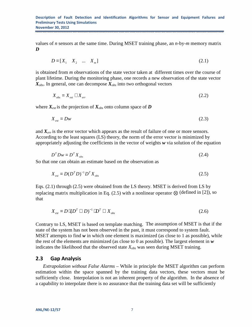
values of n sensors at the same time. During MSET training phase, an n-by-m memory matrix D 1 2[ ... ]mD X X X= (2.1) is obtained from m observations of the state vector taken at different times over the course of plant lifetime. During the monitoring phase, one records a new observation of the state vector Xobs. In general, one can decompose Xobs into two orthogonal vectors
obs est errX X X= + (2.2) where Xest is the projection of Xobs onto column space of D
estX Dw= (2.3) and Xerr is the error vector which appears as the result of failure of one or more sensors. According to the least squares (LS) theory, the norm of the error vector is minimized by appropriately adjusting the coefficients in the vector of weights w via solution of the equation
T T
obsD Dw D X= (2.4) So that one can obtain an estimate based on the observation as
1( )T Test obsX D D D D X−= (2.5)
Eqs. (2.1) through (2.5) were obtained from the LS theory. MSET is derived from LS by replacing matrix multiplication in Eq. (2.5) with a nonlinear operator ⊗ (defined in [2]), so that
1( )T Test obsX D D D D X−= ⋅ ⊗ ⋅ ⊗ (2.6)
Contrary to LS, MSET is based on template matching. The assumption of MSET is that if the state of the system has not been observed in the past, it must correspond to system fault. MSET attempts to find w in which one element is maximized (as close to 1 as possible), while the rest of the elements are minimized (as close to 0 as possible). The largest element in w indicates the likelihood that the observed state Xobs was seen during MSET training.
2.3 Gap Analysis
Extrapolation without False Alarms – While in principle the MSET algorithm can perform estimation within the space spanned by the training data vectors, these vectors must be sufficiently close. Interpolation is not an inherent property of the algorithm. In the absence of a capability to interpolate there is no assurance that the training data set will be sufficiently

Description of Fault Detection and Identification Algorithms for Sensor and Equipment Failures and
Preliminary Tests Using Simulations 8 November 30, 2012 dense to populate the entire normal operation region. So there is a need for MSET-type state estimation that can more reliably cover normal operation from the standpoint of interpolation.
With no formal basis for interpolation, extrapolation by analog is similarly deficient.
Without a means for even mild extrapolation beyond the training data set, small changes in normal operation can take the system outside of the learned region and give rise to a false alarm. Thus, false alarms are a “way of life”. [3, 4]
Dynamic State Estimation – The absence in MSET of a transient estimation capability rules out the detection of sensor or component faults that are observable as anomalies only in transient data. For example, the degradation of the time response of an RTD is observable only in the dynamic response of the device. Similarly wear in mechanical components can result in anomalous force amplification during changes in load (compared to steady state operation). So wear may go initially undetected during steady-state operation until later when wear has advanced sufficiently to result in unexpected catastrophic failure.
In particular, the MSET algorithm has no mechanism for learning the relationship among
process variables during a transient. A transient excites dynamics that create new relationships between inputs and outputs that do not exist during steady state. Since there is no mechanism for learning these relationships, dynamics that are excited can result in estimation error and lead to false alarms in fault detection applications. One might alternately explicitly account for the error caused by the excited modes by widening the uncertainty threshold, but the detection sensitivity goes down as a result.
2.4 New Algorithm: AFTR-MSET
This report describes results from a new data-driven Algorithm for Transient Multivariable Sensor Estimation (AFTR-MSET) developed in a companion NEET ASI project [5] to address the above limitations. The method [6] starts with a representation of the conservation laws for the physical system written as a set of ordinary differential equations. This model does not need to be known in detail, but some understanding of its general structure proves helpful for developing a robust data-driven model. Conditions that the training data must satisfy are then derived that ensure a reliable and robust data-driven model. This model serves as a basis for performing state estimation and for detecting failing sensors. The development also makes evident how the reliability of a data-driven model is inherently limited when it is obtained without regard to the properties of the physical system.
A theoretical underpinning lends rigor to new capabilities. The approach formally treats storage effects that give rise to dynamic excitation of the states of the system. While the system states are not necessarily measured they leave their mark as time lagged correlations in the measured process variables. A suitable lagged set of measurements implicitly contains this state information and a memory matrix that contains this data is able to represent the effect of state excitation.
The new capabilities are listed below. Only the first capability has been demonstrated, and
then through simulation. Initial results are presented in Subsection 2.6 of this report. The

Description of Fault Detection and Identification Algorithms for Sensor and Equipment Failures and
Preliminary Tests Using Simulations
November 30, 2012
ANL/NE-12/57 9
remaining capabilities are predicted based on theoretical properties. They too will be demonstrated through simulations.
• A capability to perform state estimation during dynamic excited transients and a sensor
has failed or degraded.
• A capability to perform a degree of extrapolation sufficient to solve the false alarm problem associated with newly arrived normal-operation data that lies outside the range of learned data.
• Identification of the conditions necessary for determining whether the data-driven model has properly captured causality between the inputs that drive a physical system and the outputs of the system as observed through a sensor set.
• A method to manage strong non-linearities that exceed the capabilities of a single data-driven model.
Using System Basis for Estimation - In order to formulate a computationally-efficient algorithm, we return to Eq. (2.5) in the Least Squares (LS)/MSET formulation. Instead of the entire memory matrix D we use a matrix A where the projection of the observed vector on the column space of A is
estX Aw= (2.6) (2.6) The error vector is err obs estX X X= − (2.7) where T
obsw A X= (2.8) so that
Test obsX AA X= (2.9)
Eq. (2.9) is the LS estimation using the system basis. The error vector is of the form
1 2[ ]Terr nX e e e= ⋯ . (2.10)
From empirical knowledge of the NPP, we know that among the n sensors installed at NPP, only a small number will fail at any given time. Therefore, we expect that using the L2 norm, one will detect sensor fault, but will not attribute the error correctly to the “faulty” sensor.
Description of Fault Detection and Identification Algorithms for Sensor and Equipment Failures and
Preliminary Tests Using Simulations 10 November 30, 2012
To correctly detect and identify sensor fault, we propose an error vector of the form
[ ]0 0T
err iX e= ⋯ ⋯ . (2.13) The location of the non-zero error ei, i.e. the value of index i is not known a-priori. The number i will be identified when the search routine returns the error vector of the form in Eq. (2.13). By analogy with statistical mechanics, we choose a norm that minimizes the entropy of the error vector Xerr. In general, entropy of any system is proportional to the log of the number of filled states. We can view the n elements of Xerr as the number of available states (boxes) to be filled with non-zero entries. Using an appropriate norm minimization we allow an arbitrarily large number to be assigned to ei (i.e. fill the i th box) on the condition that all other states remain empty.
In practice, one might not obtain “exact” zeros in Eq. (2.13). Instead, one should set the tolerance level, i.e., a small number ε, such that any number smaller than ε would be considered as a “zero.”
2.5 Models
2.5.1 Resistance Temperature Detector
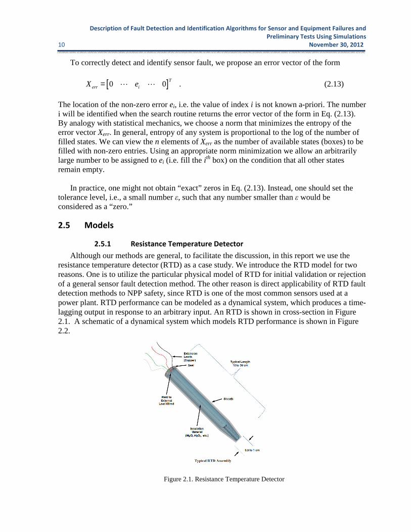
Although our methods are general, to facilitate the discussion, in this report we use the resistance temperature detector (RTD) as a case study. We introduce the RTD model for two reasons. One is to utilize the particular physical model of RTD for initial validation or rejection of a general sensor fault detection method. The other reason is direct applicability of RTD fault detection methods to NPP safety, since RTD is one of the most common sensors used at a power plant. RTD performance can be modeled as a dynamical system, which produces a time-lagging output in response to an arbitrary input. An RTD is shown in cross-section in Figure 2.1. A schematic of a dynamical system which models RTD performance is shown in Figure 2.2.
Figure 2.1. Resistance Temperature Detector
Description of Fault Detection and Identification Algorithms for Sensor and Equipment Failures and
Preliminary Tests Using Simulations
November 30, 2012
ANL/NE-12/57 11
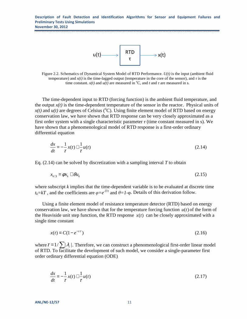
Figure 2.2. Schematics of Dynamical System Model of RTD Performance. U(t) is the input (ambient fluid
temperature) and x(t) is the time-lagged output (temperature in the core of the sensor), and τ is the time constant. x(t) and u(t) are measured in oC, and t and τ are measured in s.
The time-dependent input to RTD (forcing function) is the ambient fluid temperature, and the output x(t) is the time-dependent temperature of the sensor in the reactor. Physical units of x(t) and u(t) are degrees of Celsius (oC). Using finite element model of RTD based on energy conservation law, we have shown that RTD response can be very closely approximated as a first order system with a single characteristic parameter τ (time constant measured in s). We have shown that a phenomenological model of RTD response is a first-order ordinary differential equation
1 1( ) ( )
dxx t u t
dt τ τ= − +
(2.14)
Eq. (2.14) can be solved by discretization with a sampling interval T to obtain
1k k kx x uφ θ+ = + (2.15)
where subscript k implies that the time-dependent variable is to be evaluated at discrete time tk=kT , and the coefficients are φ=e-T/τ and θ=1-φ. Details of this derivation follow.
Using a finite element model of resistance temperature detector (RTD) based on energy conservation law, we have shown that for the temperature forcing function ( )u t of the form of the Heaviside unit step function, the RTD response ( )x t can be closely approximated with a single time constant
/( ) (1 )tx t C e τ−= − (2.16)
where 1/ | |iτ λ= ∑ . Therefore, we can construct a phenomenological first-order linear model of RTD. To facilitate the development of such model, we consider a single-parameter first order ordinary differential equation (ODE)
1 1
( ) ( )dx
x t u tdt τ τ
= − + (2.17)

Description of Fault Detection and Identification Algorithms for Sensor and Equipment Failures and
Preliminary Tests Using Simulations 12 November 30, 2012
which is a particular example of a general first order constant-coefficient linear system with a forcing function
( ) ( )dx
Ax t Bu tdt
= + (2.18)
where ( )x t is the state vector, and ( )u t is the input signal. Eq. (2.18) has the general solution
0 0( ) ( ) ( ) ( ) ( )o
t
tx t t t x t B t u dφ φ ξ ξ ξ= − + −∫ (2.19)
where ���� is the state transition matrix, which is the solution of the homogeneous ODE Eq. (2.18)
( )d
A tdt
φ φ= (2.20)
so that ( ) Att eφ = (2.21) In the RTD model 1/A τ= − and 1/B τ= , so that
/( ) tt e τφ −= (2.22)
Then
0
0
/( )/ /
0( ) ( ) ( )t tt t
t
ex t e x t e u d
ττ ξ τ ξ ξ
τ
−− −= + ∫ (2.23)
If the initial condition for Eq. (2.18) is 0 0t = and (0) 0x = , then
0
//( ) ( )
t t
t
ex t e u d
τξ τ ξ ξ
τ
−
= ∫ (2.24)
If we assume the forcing function to have the form of the scaled Heaviside unit step function with amplitude C, then the solution is
/( ) (1 )tx t C e τ−= − (2.25)
which confirms the validity of using Eq. (2.17) as a phenomenological model of RTD response. Next, we develop discrete-time solution of Eq. (2.17). We use the discrete time notation kt kT= , where T is the sampling interval. We propagate the state vector ( )x t in time
from 0 kt t kT= = to 1 ( 1)kt t k T+= = + . The sampling interval T is assumed to be small enough
Description of Fault Detection and Identification Algorithms for Sensor and Equipment Failures and
Preliminary Tests Using Simulations
November 30, 2012
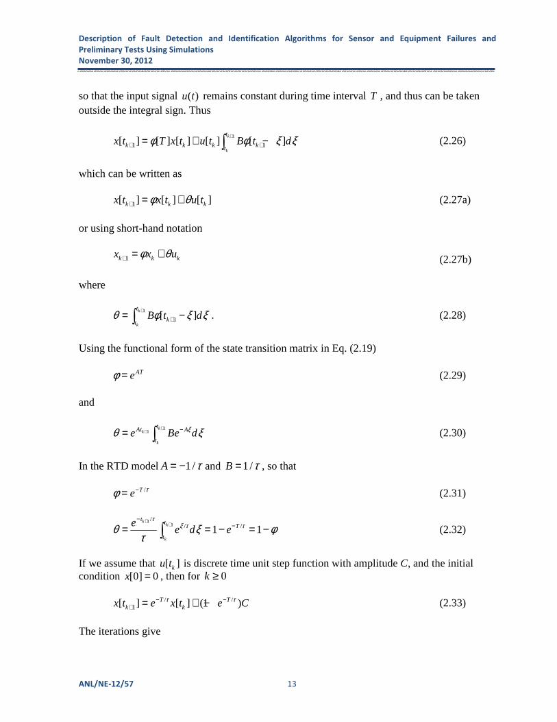
ANL/NE-12/57 13
so that the input signal ( )u t remains constant during time interval T , and thus can be taken outside the integral sign. Thus
1
1 1[ ] [ ] [ ] [ ] [ ]k
k
t
k k k ktx t T x t u t B t dφ φ ξ ξ+
+ += + −∫ (2.26)
which can be written as
1[ ] [ ] [ ]k k kx t x t u tφ θ+ = + (2.27a)
or using short-hand notation 1k k kx x uφ θ+ = + (2.27b) where
1
1[ ]k
k
t
ktB t dθ φ ξ ξ+
+= −∫ . (2.28)
Using the functional form of the state transition matrix in Eq. (2.19) ATeφ = (2.29) and
1
1k
k
k
tAt A
te Be dξθ ξ+
+ −= ∫ (2.30)
In the RTD model 1/A τ= − and 1/B τ= , so that
/Te τφ −= (2.31)
11
// /1 1
kk
k
t tT
t
ee d e
τξ τ τθ ξ φ
τ+
+−
−= = − = −∫ (2.32)
If we assume that [ ]ku t is discrete time unit step function with amplitude C, and the initial condition [0] 0x = , then for 0k ≥ / /
1[ ] [ ] (1 )T Tk kx t e x t e Cτ τ− −
+ = + − (2.33)
The iterations give

Description of Fault Detection and Identification Algorithms for Sensor and Equipment Failures and
Preliminary Tests Using Simulations 14 November 30, 2012
/
2 /
3 /
//
[ ] (1 )
[2 ] (1 )
[3 ] (1 )
[ ] [ ] (1 ) (1 )k
T
T
T
tkTk
x T C e
x T C e
x T C e
x t x kT C e C e
τ
τ
τ
ττ
−
−
−
−−
= −= −= −
= = − = −
⋮
(2.34)
Thus we obtain the discrete time analog of the continuous time solution in Eq. (2.25).
A sensor at a nuclear power plant (NPP) consists of a sensing element, which is directly in contact with the thermal fluid, and an electronic module, which is connected to the sensing element but physically located outside of the cooling system. Physical degradation of an RTD sensing element manifests itself in slower sensor response, i.e., increase in the value of τ. According to Nuclear Regulatory Commission (NRC) regulations, an RTD is considered to be defective if its time constant approximately doubles. The change in τ cannot be inferred from steady-state observation because in the steady state, the RTD output is not related to τ but to the amplitude of the forcing function. Therefore, fault detection which relies on steady-state measurements will detect sensor failure only if the sensor stops responding altogether. The time constant can potentially be obtained from the dynamic response of the sensor. In addition to sensing element degradation, other sources of measurement faults include noise in the electronic module. In this project, we have investigated detection of sensor faults caused by both the sensing element and the electronic module.
In a power plant, sensors are typically placed at the input and output legs of a component
of the plant cooling system, which has at least one input and one output. Therefore, sensors, in general are correlated in time. A general schematic drawing of two correlated sensors is shown in Figure 2.3. Sensors 1 and 2 have inputs u1(t) and u2(t), and corresponding outputs x1(t) and x2(t). Sensors 1 and 2 are defined to be correlated if the inputs u1(t) and u2(t) are correlated. For
Figure 2.3. Dynamics of Two Correlated Sensors. Sensors 1 and 2 inputs u1(t) and u2(t), and corresponding
outputs x1(t) and x2(t). Correlation between u1(t) and u2(t) is provided by the dynamical response of the Component, which has u1(t) and u2(t) as input and output.
Description of Fault Detection and Identification Algorithms for Sensor and Equipment Failures and
Preliminary Tests Using Simulations
November 30, 2012
ANL/NE-12/57 15
the Component in Figure 2.3, u1(t) is the input, and u2(t) is the output. The correlation function between u1(t) and u2(t) is provided by the response of the Component, which itself is a dynamical system. In the simplest case, the Component is an Identity, i.e., u1(t) = u2(t). A physical example of such a case may be represented by two RTDs located next to each other in a straight section of pipe.
2.5.2 Printed Circuit Heat Exchanger
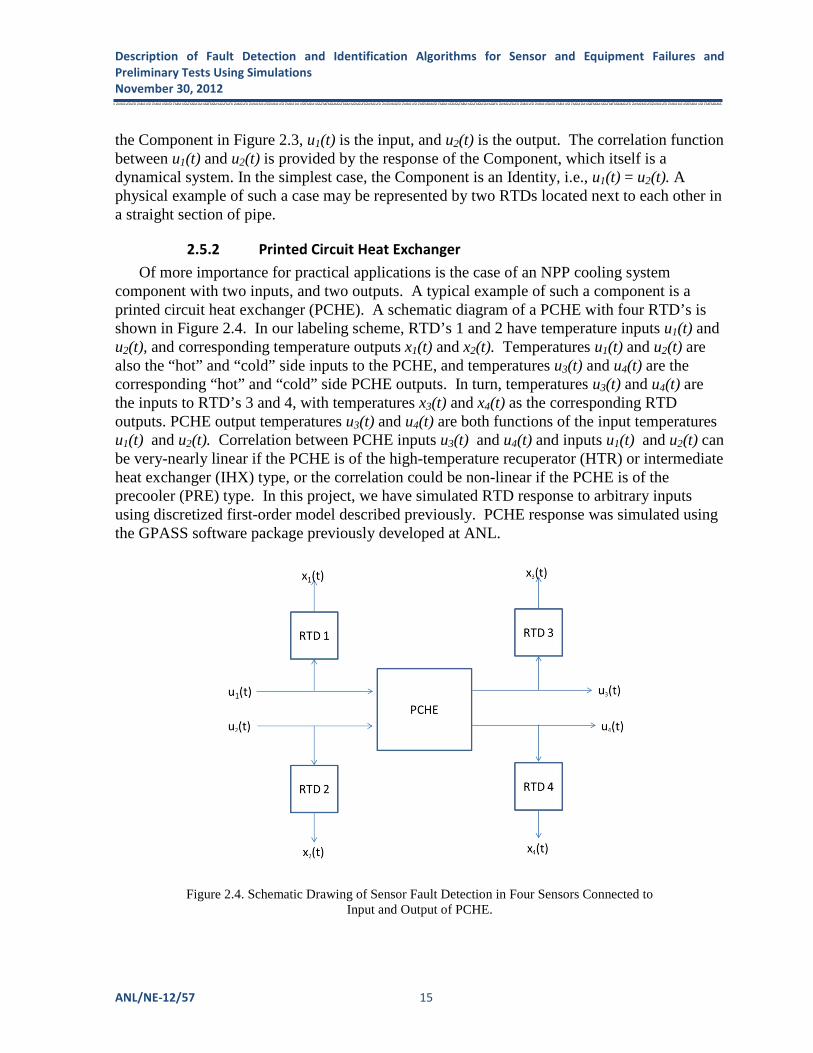
Of more importance for practical applications is the case of an NPP cooling system component with two inputs, and two outputs. A typical example of such a component is a printed circuit heat exchanger (PCHE). A schematic diagram of a PCHE with four RTD’s is shown in Figure 2.4. In our labeling scheme, RTD’s 1 and 2 have temperature inputs u1(t) and u2(t), and corresponding temperature outputs x1(t) and x2(t). Temperatures u1(t) and u2(t) are also the “hot” and “cold” side inputs to the PCHE, and temperatures u3(t) and u4(t) are the corresponding “hot” and “cold” side PCHE outputs. In turn, temperatures u3(t) and u4(t) are the inputs to RTD’s 3 and 4, with temperatures x3(t) and x4(t) as the corresponding RTD outputs. PCHE output temperatures u3(t) and u4(t) are both functions of the input temperatures u1(t) and u2(t). Correlation between PCHE inputs u3(t) and u4(t) and inputs u1(t) and u2(t) can be very-nearly linear if the PCHE is of the high-temperature recuperator (HTR) or intermediate heat exchanger (IHX) type, or the correlation could be non-linear if the PCHE is of the precooler (PRE) type. In this project, we have simulated RTD response to arbitrary inputs using discretized first-order model described previously. PCHE response was simulated using the GPASS software package previously developed at ANL.
Figure 2.4. Schematic Drawing of Sensor Fault Detection in Four Sensors Connected to
Input and Output of PCHE.

Description of Fault Detection and Identification Algorithms for Sensor and Equipment Failures and
Preliminary Tests Using Simulations 16 November 30, 2012
2.6 Algorithm Results
2.6.1 MSET - Application to Monitoring Dynamic Sensor Response
MSET operates by comparing a new measurement against the existing database, and has no capacity to generalize. Therefore, MSET accuracy depends entirely on the content of the training data. In general, the larger the size of the training data, the more accurate MSET performance would be. The size of the data which can be used for MSET training, aside from the obvious limited volume of recorded data, is also limited by sensor’s lifetimes. That is, NPP data recorded over a timespan larger than the sensor’s lifetime may contain readings from failed sensors. The implicit assumption in MSET is that the state vector of NPP sensors has only a finite number of “normal” states. That is, all “normal” states of the NPP cooling system can be learned from a reasonably small amount of training data. This assumption might be justified if MSET is to be used for monitoring of steady-state observations. During normal NPP operation, temperature, pressure and flow rate of the cooling fluid do not change frequently. Thus, it is very likely that all “normal” steady states of the state vector can be learned from several years-worth of training data. On the other hand, transitions between steady states can occur via a variety of transients. In general, the plant is seldom at steady state since it is either purposefully undergoing a normal operational transient or undergoing an unexpected upset transient. Even when the plant is nominally at steady state, control system dead band may result in small transients as controlled variables alternately drift between dead band limits. In order to learn all possible transients of NPP cooling system, MSET may need to be trained on an excessively large database of prior measurements. Even if such database becomes available, this places a computational burden of inverting the memory matrix consisting of possibly millions of elements.
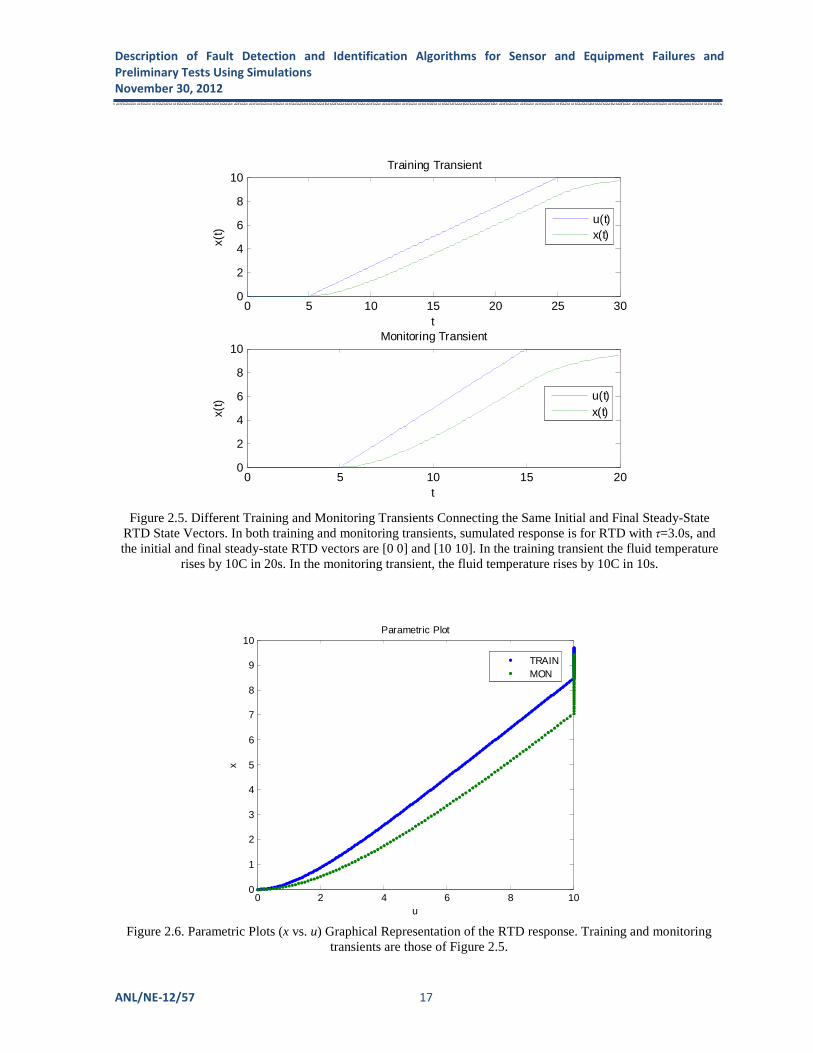
An example of two different transients connecting the same steady states is shown in
Figure 2.5. The top panel displays training transient during which fluid temperature rises by 10C in 20s. The bottom panel displays a monitoring transient during which fluid temperature rises by 10C in 10s. RTD response output temperature is calculated in both cases using τ=3.0s and T=0.1s. In the MSET formalism, the state vector of RTD is a time-dependent 2-by-1 vector of the input and output temperatures X(t)=[ x(t) u(t)] T. All training and monitoring states of the RTD can be displayed graphically as points on a 2-D plane. RTD training and monitoring states of Figure 2.5 are plotted as parametric curves of output vs. input temperatures in Figure 2.6. As can be seen from either Figure 2.5 or Figure 2.6, both the training and monitoring transients connect initial and final steady states (0,0) and (10,10). All the points on the training and monitoring transients for t<5s in Figure 2.5 map to the point (0,0) in Figure 2.6. Training transient points for 5s<t<25s and monitoring transient points for 5s<t<15s map to two different parametric curves in Figure 2.6. Training transient points for t>25s and monitoring transient points for t>15s in Figure 2.5 map to the vertical line intersecting the horizontal axis at Tin = 10C in Figure 2.6.
Description of Fault Detection and Identification Algorithms for Sensor and Equipment Failures and
Preliminary Tests Using Simulations
November 30, 2012
ANL/NE-12/57 17
Figure 2.5. Different Training and Monitoring Transients Connecting the Same Initial and Final Steady-State RTD State Vectors. In both training and monitoring transients, sumulated response is for RTD with τ=3.0s, and the initial and final steady-state RTD vectors are [0 0] and [10 10]. In the training transient the fluid temperature
rises by 10C in 20s. In the monitoring transient, the fluid temperature rises by 10C in 10s.
Figure 2.6. Parametric Plots (x vs. u) Graphical Representation of the RTD response. Training and monitoring transients are those of Figure 2.5.
0 5 10 15 20 25 300
2
4
6
8
10
t
x(t)
Training Transient
u(t)x(t)
0 5 10 15 200
2
4
6
8
10
t
x(t)
Monitoring Transient
u(t)x(t)
0 2 4 6 8 100
1
2
3
4
5
6
7
8
9
10
u
x
Parametric Plot
TRAINMON
Description of Fault Detection and Identification Algorithms for Sensor and Equipment Failures and
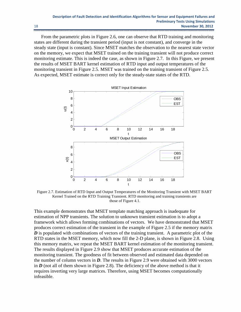
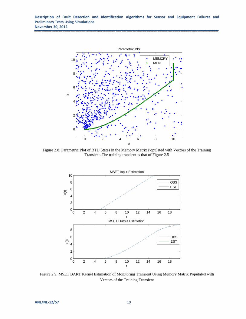
Preliminary Tests Using Simulations 18 November 30, 2012 From the parametric plots in Figure 2.6, one can observe that RTD training and monitoring states are different during the transient period (input is not constant), and converge in the steady state (input is constant). Since MSET matches the observation to the nearest state vector on the memory, we expect that MSET trained on the training transient will not produce correct monitoring estimate. This is indeed the case, as shown in Figure 2.7. In this Figure, we present the results of MSET BART kernel estimation of RTD input and output temperatures of the monitoring transient in Figure 2.5. MSET was trained on the training transient of Figure 2.5. As expected, MSET estimate is correct only for the steady-state states of the RTD.
Figure 2.7. Estimation of RTD Input and Output Temperatures of the Monitoring Transient with MSET BART Kernel Trained on the RTD Training Transient. RTD monitoring and training transients are
those of Figure 4.1. This example demonstrates that MSET template matching approach is inadequate for estimation of NPP transients. The solution to unknown transient estimation is to adopt a framework which allows forming combinations of vectors. We have demonstrated that MSET produces correct estimation of the transient in the example of Figure 2.5 if the memory matrix D is populated with combinations of vectors of the training transient. A parametric plot of the RTD states in the MSET memory, which now fill the 2-D plane, is shown in Figure 2.8. Using this memory matrix, we repeat the MSET BART kernel estimation of the monitoring transient. The results displayed in Figure 2.9 show that MSET produces accurate estimation of the monitoring transient. The goodness of fit between observed and estimated data depended on the number of column vectors in D. The results in Figure 2.9 were obtained with 3000 vectors in D (not all of them shown in Figure 2.8). The deficiency of the above method is that it requires inverting very large matrices. Therefore, using MSET becomes computationally infeasible.
0 2 4 6 8 10 12 14 16 180
2
4
6
8
10
t
u(t)
MSET Input Estimation
OBSEST
0 2 4 6 8 10 12 14 16 180
2
4
6
8
t
x(t)
MSET Output Estimation
OBSEST
Description of Fault Detection and Identification Algorithms for Sensor and Equipment Failures and
Preliminary Tests Using Simulations
November 30, 2012
ANL/NE-12/57 19
Figure 2.8. Parametric Plot of RTD States in the Memory Matrix Populated with Vectors of the Training
Transient. The training transient is that of Figure 2.5
Figure 2.9. MSET BART Kernel Estimation of Monitoring Transient Using Memory Matrix Populated with
Vectors of the Training Transient
0 2 4 6 8 10
0
2
4
6
8
10
u
x
Parametric Plot
MEMORYMON
0 2 4 6 8 10 12 14 16 180
2
4
6
8
10
t
u(t)
MSET Input Estimation
OBSEST
0 2 4 6 8 10 12 14 16 180
2
4
6
8
t
x(t)
MSET Output Estimation
OBSEST

Description of Fault Detection and Identification Algorithms for Sensor and Equipment Failures and
Preliminary Tests Using Simulations 20 November 30, 2012
2.6.2 AFTR-MSET
Fault Detection in a System of Two Correlated RTD’s Using Training Vectors and Proprietary Norm - As discussed in Section 2.5.1, the simplest case of two correlated RTD’s monitoring temperature input and output of a Component is when the Component is an Identity, i.e., u1(t) = u2(t) in Figure 2.3. A physical example of such case may be represented by two RTDs located next to each other in a straight section of pipe. A schematic diagram of such scenario is shown in Figure 2.10. The RTD’s 1 and 2 with respective temperature outputs x1(t) and x2(t) are driven by the same forcing function temperature u(t). In the training transient shown in Figure 2.11, both RTD’s are “normal” with τ1= τ2=3.0s.In the monitoring transient, we introduce sensor fault in RTD1 by choosing τ1=6.0s, while RTD2 is “normal” with τ2=3.0s. Figures 2.12 and 2.13 display the result of sensor estimation using a basis learned from the training transient. In Figure 2.12, the fault is detected with L2 norm minimization, but the error is incorrectly attributed to both RTD’s. In Figure 2.13, fault is detected with the proprietary norm minimization, and the error is correctly attributed to the “faulty” RTD1. In the proprietary norm estimation, the tolerance was set to ε=10-5. This example demonstrates the validity of our hypothesis of detection and attribution of sensor fault.
Figure 2.10. Schematic Diagram of Two Correlated RTD’s Driven by the Same Forcing Function. RTDs 1 and 2
with outputs x1(t) and x2(t) are driven by the same forcing function u(t).

Description of Fault Detection and Identification Algorithms for Sensor and Equipment Failures and
Preliminary Tests Using Simulations
November 30, 2012
ANL/NE-12/57 21
Figure 2.11. Training and Monitoring Transients for Fault Detection in a System of Two Correlated RTD’s. In the training transient, τ1=τ2=3.0s. In the monitoring transient τ1=6.0s (defective RTD) and τ2=3.0s.
Figure 2.12. Estimation of Two RTD’s with L2 Norm and Vectors Learned from the Training Data. In the
minimized L2 norm estimation, we minimize the square of the error vector. While RTD1 is “normal” and RTD2 is “fault”, minimization of L2 norm detects the fault but incorrectly attributes the error to both RTD’s.

Description of Fault Detection and Identification Algorithms for Sensor and Equipment Failures and
Preliminary Tests Using Simulations 22 November 30, 2012
Figure 2.13. Estimation of Two RTD’s with Proprietary Norm Minimization and Vectors Learned from Training Data.
Fault Detection in HTR Using Training Vectors and Proprietary Norm - Subsection 2.5.2 describes the general case of four correlated RTD’s monitoring two inputs and two outputs of a PCHE (see Figure 2.4). Presently, we have investigated a simplified scenario, in which temperatures at the input and output of a PCHE were assumed to be monitored directly (without RTD’s).
The PCHE in our study was a high-temperature recuperator (HTR) with CO2 as a working fluid. Schematic diagram of HTR dynamics with HOT and COLD inputs u1(t) and u2(t) and
Figure 2.14. A schematic Diagram of HTR Dynamics with HOT and COLD Inputs and Outputs. HOT and COLD
inputs are u1(t) and u2(t), and HOT and COLD outputs x1(t) and x2(t).

Description of Fault Detection and Identification Algorithms for Sensor and Equipment Failures and
Preliminary Tests Using Simulations
November 30, 2012
ANL/NE-12/57 23
HOT and COLD outputs x1(t) and x2(t) is shown in Figure 2.14. The correlation between HTR inputs was calculated with GPASS code in the quasi-static mode (energy and mass storage was turned off). We considered two separate cases: (1) u1(t) is changing while u2(t) remains constant, (2) both u1(t) and u2(t) are changing. In both cases, a sensor fault was simulated by adding a constant baseline shift of 1oC to the COLD sensor output x2(t).
In the HTR system, there are two dependent and two independent variables. Therefore, the rank of the basis cannot be larger than two. However, numerical calculations of the basis of the training transient have indicated that the basis is full rank. We explain this inconsistency by the presence of mild nonlinearities in the HTR response. We use rank one approximation of the training vectors
Figure 2.15 shows the training and monitoring transients for the case of only one input changing. Non-zero singular values of the training transient are σ1=104.08791, σ2=0.0512 and σ3=0.0006. Since σ1/ σ2 >1e3, we obtained an approximation of the training data using rank one SVD approximation. Sensor fault detection and attribution is shown in Figure 2.16. Using the proprietary norm minimization, the fault was correctly attributed to the COLD output. Estimation with the proprietary norm minimization requires setting the value of tolerance to classify a number as a zero. Tolerance is related to nonlinearity of the system, so it is a function of transient amplitude. Thus tolerance may need to be estimated from both the training data and the monitoring data. In this example, the tolerance was ε=0.01.
Figure 2.15. Training and Monitoring Transients for One Input and Two Outputs (HOT and COLD) of HTR. In this for the case, one HTR input is changing and another input is stationary. Fault is introduced as a 1C baseline
shift in the COLD output of HTR.
0 50 100 150 2000
10
20
IN
TRAINMON
0 50 100 150 200-0.5
0
0.5
1
HO
T
TRAINMON
0 50 100 150 200-10
0
10
20
CO
LD
TRAINMON
0 50 100 150 2000
10
20
IN
TRAINMON
0 50 100 150 200-0.5
0
0.5
1
HO
T
TRAINMON
0 50 100 150 200-10
0
10
20
CO
LD
TRAINMON
0 50 100 150 2000
10
20
IN
TRAINMON
0 50 100 150 200-0.5
0
0.5
1
HO
T
TRAINMON
0 50 100 150 200-10
0
10
20
CO
LD
TRAINMON

Description of Fault Detection and Identification Algorithms for Sensor and Equipment Failures and
Preliminary Tests Using Simulations
24 November 30, 2012
Figure 2.16. Fault Detection and Attribution with the Vectors Learned from the Training Data and Proprietary Norm Minimization. The error is correctly attributed to the COLD output.
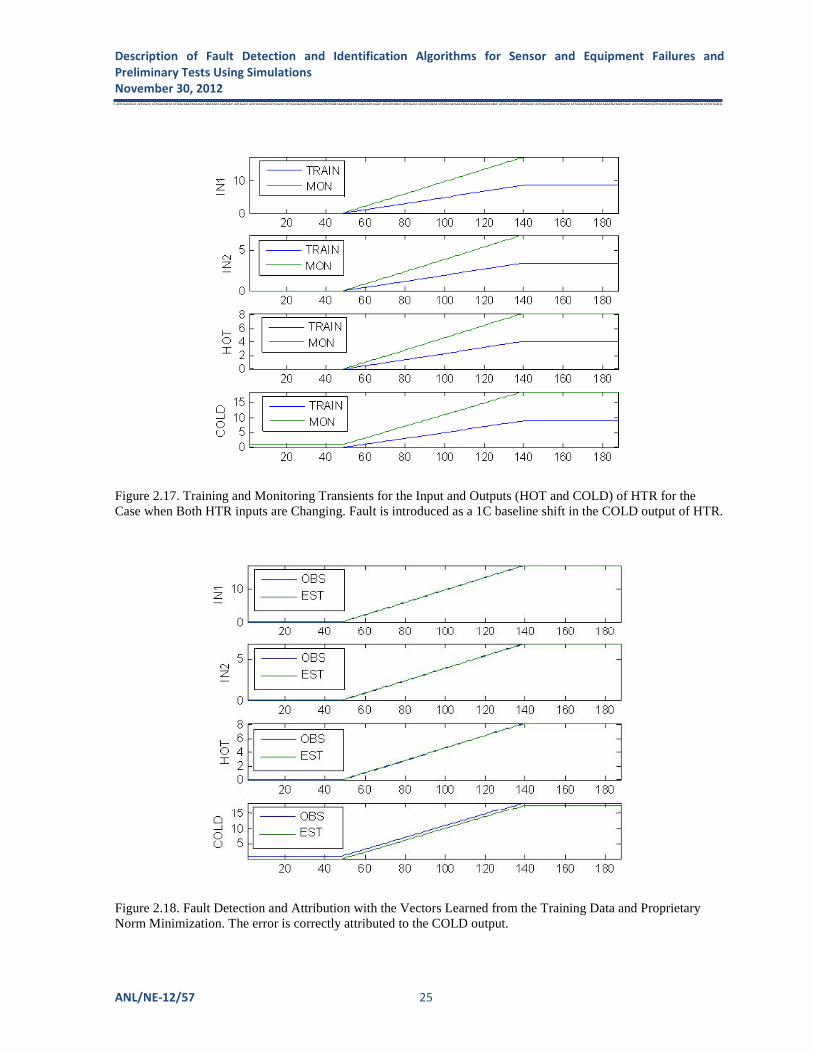
Figure 2.17 shows the training and monitoring transients for the case of both outputs changing. Non-zero singular values of the training transient are σ1=119.0836, σ2=0.0852, σ3=0.0229, and σ4=0.0053. Again, since σ1/ σ2 >1e3, we obtained a linear approximation of the vector training data using rank one SVD approximation. Sensor fault detection and attribution is shown in Figure 2.18. HTR nonlinearity with both inputs changing was slighter stronger compared to the case of only one input changing. For the RTD estimation in Figure 2.18, tolerance was set to ε=0.05.
Description of Fault Detection and Identification Algorithms for Sensor and Equipment Failures and
Preliminary Tests Using Simulations
November 30, 2012
ANL/NE-12/57 25
Figure 2.17. Training and Monitoring Transients for the Input and Outputs (HOT and COLD) of HTR for the Case when Both HTR inputs are Changing. Fault is introduced as a 1C baseline shift in the COLD output of HTR.
Figure 2.18. Fault Detection and Attribution with the Vectors Learned from the Training Data and Proprietary Norm Minimization. The error is correctly attributed to the COLD output.
Description of Fault Detection and Identification Algorithms for Sensor and Equipment Failures and
Preliminary Tests Using Simulations 26 November 30, 2012
3. Component Fault Identification
Diagnosing an equipment fault differs in a fundamental way from diagnosing a sensor fault. A corrupted sensor output can be detected using the analytic methods of Section 2 without the need for complex reasoning. Only a representation for the normal operating state of the system is needed. An equipment fault, on the other hand, involves a redirection of mass, energy, or momentum as a consequence of a physical change in the system from normal. For fault diagnosis to proceed there needs to be some reasoning process that can relate observed changes in process variables back to a physical change in the system.
It is important that sensors are validated before an equipment fault diagnosis proceeds.
The methods of the previous section provide such a capability.
3.1 Background
The methods and algorithms of the PRODIAG code [7] were developed to perform automated diagnosis of faults in nuclear power plants. Data from plant sensors are sampled periodically and trends are compared against the steady-state condition to determine if an anomaly exists. If an anomaly is detected, the code attempts to identify the cause through a reasoning process that involves rules that relate faults to sensor trends combined with knowledge of how plant components are connected.
The code implementation is representative of expert systems developed in the mid 1990’s.
That is, the reasoning process is intimately wedded to the execution of rules as opposed to more recent trends where the rules are presented for simultaneous execution by a reasoning engine. The code is programmed in Prolog.
While the implementation of PRODIAG may be dated by today’s computer science
standards, two of the underlying methods of the code still stand as powerful and innovative. First, the rule base is formulated in a way that does not require a fault event to be hypothesized or for a fault list to be scanned exhaustively. The search procedure is not event driven but uses the qualitative reasoning of de Kleer [8,9] and consistency-based diagnosis to arrive at a fault diagnosis. This approach avoids having to a priori precompile for the system of interest an exhaustive list of faults for consideration. Second, the rules are implemented in a way that is generalized and independent of the users particular Piping Instrumentation Diagram (PID). That is, the code accepts the user’s specific PID data without the need to reformulate any of the rules. Thus, application of the code to a new application involves, in principle, only providing a new PID.
PRODIAG was tested extensively in the late 1990s on the Chemical and Volume Control System (CVCS) of the Braidwood nuclear power plant [10]. These tests involved data from the plant simulator. The tests were performed blind and without noise on the signals. The code correctly diagnosed the fault in 37 of 39 [10] transients presented to it. Figure 3.1 is a screenshot from that work where a clogged filter in the CVCS was correctly diagnosed by PRODIAG.

Description of Fault Detection and Identification Algorithms for Sensor and Equipment Failures and
Preliminary Tests Using Simulations
November 30, 2012
ANL/NE-12/57 27
Figure 3.1. Fault Diagnosis GUI Showing Clogged Filter in CVCS as Identified by PRODIAG
Work is underway on this project to bring the implementation of PRODIAG up to modern
software standards. From a developer’s standpoint the objective is to make the code more maintainable and extensible. From a production standpoint the objective is to make the code modular so that it can be seamlessly interfaced to the technology demonstration platform. The tasks for achieving this are
• Characterize and Delineate the PRODIAG Program
• Specification of New Software Architecture
• Rewrite of PRODIAG Code
• Identify Role and Use of an Open-Source Automated Reasoning Engine
3.2 Algorithms
The methods of PRODIAG as described in [10] are summarized prior to reporting progress
on the above modernization tasks. The most basic function of components in thermal-hydraulic (TH) processes is to provide
sources or sinks of mass, momentum, or energy. Once components are classified as sources or sinks of these three functions, their malfunction can be identified by detecting imbalances in the conservation of mass, momentum, and energy. The advantage of this function-oriented ap-proach stems from the relatively small number of generic types of components (e.g., pump, valve, and heat exchanger) utilized in TH processes and the fact that each component is designed to perform basically one key function. In contrast, there are hundreds or even thousands of possible modes of component failures in nuclear power plant processes.

Description of Fault Detection and Identification Algorithms for Sensor and Equipment Failures and
Preliminary Tests Using Simulations 28 November 30, 2012
PRODIAG' s reasoning is based on qualitative physics [9] where a small number of
qualitative values, such as increasing, decreasing, and unchanging trends, are used to represent the values of continuous real-valued variables. Qualitative reasoning approximates the back-of-the-envelope calculations that analysts use to confirm, semi-quantitatively, certain general numerical features of a transient response. By taking a qualitative reasoning approach, generality is gained. For example, the trend information of a flow signal can be used for diagnosis without knowledge of the exact numerical value of the flow signal and independent of the process. This advantage, however, is offset by some loss of information, which cannot be avoided.
When a component malfunctions, it causes the process TH signals, e.g., pressure, flow,
temperature, and level, to vary or trend from their expected values, producing a set of symptoms. The traditional event-oriented expert system diagnostic approach is to apply "if (symptom/condition) then (fault/consequence)" production rules to directly relate process symptoms into component faults. PRODIAG’S diagnostic strategy is carried out by separating information into three distinct but interacting knowledge bases:
1. A systematic structuring of the qualitative form of the macroscopic conservation equations
constitutes the physical rules database (PRD). 2. A functional classification of generic process components forms the component
classification dictionary (CCD). 3. The process-specific piping database (PID) information is represented in the piping and
instrumentation database (PIDB). Process symptoms are related to component faults through the three-step mapping illustrated in
Figure 3.2, where the three knowledge bases perform the following functions: 1. The PRD maps the qualitative trends in the T-H signals (e.g., increasing pressure and
decreasing flow) into function imbalance trends in the three conservation types of mass, momentum, and energy. For example, it identifies a mass decrease or a momentum increase.
2. The CCD maps the identified function imbalance type and trend into generic faulty component types (e.g., closed valve, pump, and electric heater), whose failure could have been responsible for the identified imbalance, i.e., the inadequate performance of one of the three T-H functions: mass transfer, momentum transfer, and energy transfer.
3. The PIDB containing the process schematics (PID) information is applied to match specific sensors and identify specific components from the generic faulty component types, e.g., valve, pump, and electric heater, as the possible faulty component candidates.
Through this three-step mapping, the diagnosis is transformed into a function-oriented
approach and confines the process-dependent information solely to the PIDB. The PRD and the CCD are process independent. There is no need to predefine a list of possible process component faults, and the diagnostic system can be ported across different processes/plants by incorporating the appropriate PIDB through modifications only of input data files.

Description of Fault Detection and Identification Algorithms for Sensor and Equipment Failures and
Preliminary Tests Using Simulations
November 30, 2012
ANL/NE-12/57 29
Figure 3.2. Mapping of Sensor Signals into Faulty Components through the Three Knowledge Bases of
PRODIAG
3.3 Results
This section describes progress on the four tasks listed at the end of Section 3.1.
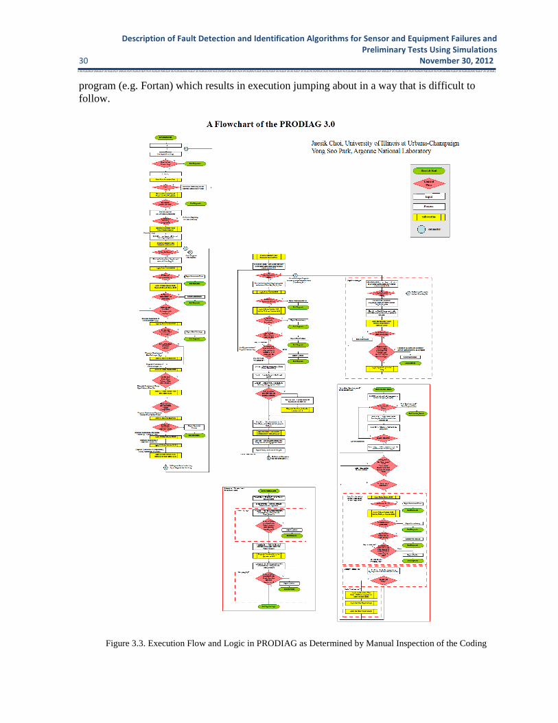
Characterize and Delineate the PRODIAG Program – An important first step was to verify that the PRODIAG coding implements the functionality defined by flowcharts in the original program documentation. The roughly 8,000 lines of Prolog code were manually inspected and the logic was newly flow charted for comparison with the original code documentation. The new flowchart is shown in Figures 3.3, albeit reduced in size to fit on a single page. The documentation effort undertaken has provided additional information on 1) detail of code structure including key variable names and logic loops, 2) inconsistencies that exist between the original flow charts and the code, 3) portions of the code that were not previously flow charted (such as the time window selector, get_data, junction search, and negative Q-logic) have now been flowcharted, 4) text descriptions of predicates present in the code but not otherwise documented, e.g. conflict resolution and junction search.
The manual inspection yielded additional findings. One is that the code does not employ object-oriented programming practices. This stems in part from the fact that standard Prolog does not support object-oriented coding. As a result the code is not structured in a way that makes it easy to read. The code as written in Prolog reads like a procedural-based
Description of Fault Detection and Identification Algorithms for Sensor and Equipment Failures and
Preliminary Tests Using Simulations 30 November 30, 2012 program (e.g. Fortan) which results in execution jumping about in a way that is difficult to follow.
Figure 3.3. Execution Flow and Logic in PRODIAG as Determined by Manual Inspection of the Coding

Description of Fault Detection and Identification Algorithms for Sensor and Equipment Failures and
Preliminary Tests Using Simulations
November 30, 2012
ANL/NE-12/57 31
Forward Evaluation
Backward Evaluation
Figure 3.4. Comparison of Diagnoses Based on Forward-Chaining and Backward-Chaining Rule Evaluation
Additionally, PRODIAG by nature of its Prolog implementation performs a diagnosis
through a rule-evaluation algorithm that is essentially hardcoded for the current PRODIAG rule set. This makes maintenance of existing rules and the addition of new rules difficult. The main difficulty is that Prolog is better suited for backward-chaining of rules whereas many of our confluence rules exist in forward-chaining form. These two types of rule evaluation are illustrated in Figure 3.4.

Description of Fault Detection and Identification Algorithms for Sensor and Equipment Failures and
Preliminary Tests Using Simulations 32 November 30, 2012
Additionally, there is a significant amount of legacy code which under the procedural-
based coding approach results in poor readability. Utility modules exist in PRODIAG for performing lower-level functions and these modules tend to be dispersed throughout the code and for some functions multiple-module versions exist. This has added clutter to the code. The utility modules need to be consolidated in a library. The occurrence of multiple-versions arising from either a lack of programming generality (i.e. hardwiring) or a sequence of poorly maintained revisions needs to be addressed. Order needs to be brought to this conglomeration that has evolved over time.
Specification of New Software Architecture – The above findings were considered in the selection of a preferred language for the re-write of the PRODIAG software.
Different programming languages and automated reasoning environments were judged for
their suitability for use in the re-write. Considered was support for or existence of 1) an inference capability, 2) object-oriented capability, 3) debugger, 4) semi-natural English-type language, and 5) integrated development environment (IDE). The tools examined were the Max-SAT solver, the VisiRule package, PyKE, and Drools (JBoss), each of which is described below. A more detailed description of each language and the results of an evaluation performed for a simple set of rules are given in [11]. A short summary of each tool follows.
The Max-SAT [12] solver could potentially be interfaced with the current implementation
of PRODIAG in Prolog. However, such a Prolog implementation would rule out the use of many advanced language programming features, such as object-oriented models. The MAX-SAT solver is very powerful tool for realizing complex logic statements and has a very succinct syntax for representation of logic statements. While in principle it is possible to do the represent PRODIAG logic statements for submittal to the MAX-SAT solver, this will require re-writing the logic rules in conjunctive form. This is a major task and additionally yields code that is less intuitive for reading by non-experts. However, at a later time we may wish to re-write PRODIAG rules in a model-based diagnostic context. Max-SAT solver would be a good choice for that task.
The VisiRule [13] package provides a graphical programming tool, natural language-like
representations, and object-oriented models. It may also maintain the diagnostic modules in Prolog because VisiRule is built on top of Prolog. By nature of its visual rule expression, it is limited in its capacity for representing complex logic rules. VisiRule translates the users graphical input into an intermediate language that is then translated in to Prolog. The existence of the intermediate language makes the users application difficult to debug. It is sold by a UK based company, Logic Programming Associate.
PyKE [14] is a Python based rule engine. It resembles the Prolog in a sense that it
maintains the backward chaining for inference. Advantages of PyKe include a good interface to high level languages (Python) and its rule representation is intuitive. However, it has not been actively maintained since 2008.
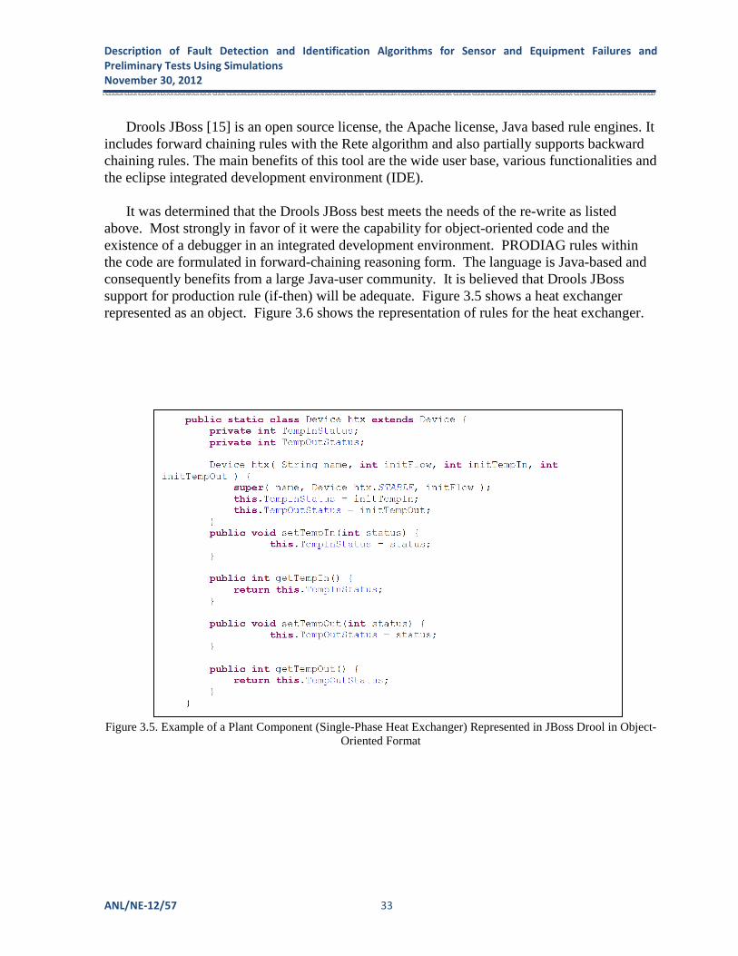
Description of Fault Detection and Identification Algorithms for Sensor and Equipment Failures and
Preliminary Tests Using Simulations
November 30, 2012
ANL/NE-12/57 33
Drools JBoss [15] is an open source license, the Apache license, Java based rule engines. It includes forward chaining rules with the Rete algorithm and also partially supports backward chaining rules. The main benefits of this tool are the wide user base, various functionalities and the eclipse integrated development environment (IDE).
It was determined that the Drools JBoss best meets the needs of the re-write as listed
above. Most strongly in favor of it were the capability for object-oriented code and the existence of a debugger in an integrated development environment. PRODIAG rules within the code are formulated in forward-chaining reasoning form. The language is Java-based and consequently benefits from a large Java-user community. It is believed that Drools JBoss support for production rule (if-then) will be adequate. Figure 3.5 shows a heat exchanger represented as an object. Figure 3.6 shows the representation of rules for the heat exchanger.
Figure 3.5. Example of a Plant Component (Single-Phase Heat Exchanger) Represented in JBoss Drool in Object-Oriented Format
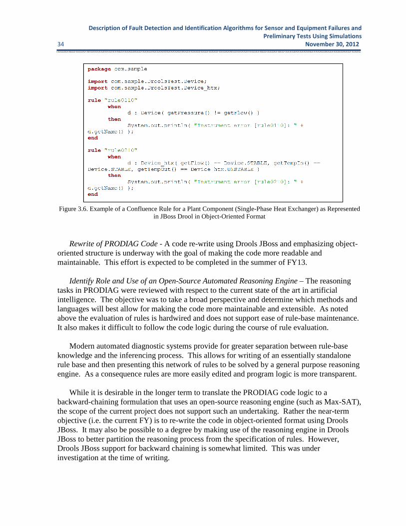
Description of Fault Detection and Identification Algorithms for Sensor and Equipment Failures and
Preliminary Tests Using Simulations 34 November 30, 2012
Figure 3.6. Example of a Confluence Rule for a Plant Component (Single-Phase Heat Exchanger) as Represented in JBoss Drool in Object-Oriented Format
Rewrite of PRODIAG Code - A code re-write using Drools JBoss and emphasizing object-
oriented structure is underway with the goal of making the code more readable and maintainable. This effort is expected to be completed in the summer of FY13.
Identify Role and Use of an Open-Source Automated Reasoning Engine – The reasoning
tasks in PRODIAG were reviewed with respect to the current state of the art in artificial intelligence. The objective was to take a broad perspective and determine which methods and languages will best allow for making the code more maintainable and extensible. As noted above the evaluation of rules is hardwired and does not support ease of rule-base maintenance. It also makes it difficult to follow the code logic during the course of rule evaluation.
Modern automated diagnostic systems provide for greater separation between rule-base
knowledge and the inferencing process. This allows for writing of an essentially standalone rule base and then presenting this network of rules to be solved by a general purpose reasoning engine. As a consequence rules are more easily edited and program logic is more transparent.
While it is desirable in the longer term to translate the PRODIAG code logic to a
backward-chaining formulation that uses an open-source reasoning engine (such as Max-SAT), the scope of the current project does not support such an undertaking. Rather the near-term objective (i.e. the current FY) is to re-write the code in object-oriented format using Drools JBoss. It may also be possible to a degree by making use of the reasoning engine in Drools JBoss to better partition the reasoning process from the specification of rules. However, Drools JBoss support for backward chaining is somewhat limited. This was under investigation at the time of writing.
Description of Fault Detection and Identification Algorithms for Sensor and Equipment Failures and
Preliminary Tests Using Simulations
November 30, 2012
ANL/NE-12/57 35
4. Automation and Fault Recovery
Plant performance improvements may be achievable through the use of automation that addresses grid and plant events that presently result in unwanted transients that can challenge the protection system. The sensor fault estimation and component fault identification methods of the previous sections provide high assurance that the plant condition is known providing an opportunity for more refined control as is achievable through automation.
4.1 Background
Automation can improve the resilience of the plant to faults. Compared to an operator it can take the plant to an acceptable state more quickly and with greater precision. It can be used to control the alignment of equipment so that temporary imbalances in heat generation and heat removal are absorbed so that a transient can be transitioned without exceeding safety settings. In existing plants there is the opportunity to absorb the excess heat generation following a disconnect from the grid by coordinated control of balance-of-plant equipment including the steam generator, bypass system, and feed water equipment.
Computer-based lookup procedures have the potential to shorten the time bottleneck by
avoiding the need to find and then leaf through the appropriate physical document. The speed with which human operators can make control-action decisions and progress through a procedure in response to an identified fault - observing all the “procedure adherence” expectations to avoid human error - has an impact on plant resilience. Control actions executed in a timely manner and based on an understanding of the evolving situation before the plant state encroaches on safety settings will increase plant resilience. Ready access to procedures and to planning tools that provide trends and can project ahead based on proposed control actions support this goal.
4.2 Advanced Control Techniques
In addition to simply automating the execution of a procedure, there is potential for more innovative applications of control technology to increase plant resilience.
Adaptive control involves automatically adjusting the response characteristics of a controller (e.g. gain constants of a PID controller) based on the plant operating state. This capability can provide greater resilience during off-normal transients. For example, in existing plants control of the steam generator is achieved using controllers that have fixed gains over the range of operation. The values for the gains are optimized for operation at the full-power condition. As a consequence for events such as grid disturbances that excite dynamics resulting from large temporary energy imbalances that take the plant away from the normal operating state, there is a greater likelihood of a reactor trip. If the controllers were able to sense the plant condition and adapt their gains to provide a more damped overall plant response, then the likelihood of a trip would be reduced.
Description of Fault Detection and Identification Algorithms for Sensor and Equipment Failures and
Preliminary Tests Using Simulations 36 November 30, 2012
Another example of adaptive control involves a failure of the grid. With the plant islanded,
the object is to increase the ability of the steam generator to temporarily absorb and store heat, then releasing the heat by steam flow through the limited capacity atmospheric dump and turbine bypass valves. The steam generator would continue to be supplied with a high rate of feed water up to a fairly high indicated water level rather than reducing feed water flow. This would require changing the feed water level algorithm to level-dominant rather dependant on the difference between feed water flow and steam flow.
Anticipatory control involves having the plant control system for severe disturbances and grid blackouts put the plant on a trajectory that anticipates the final desired power level and plant configuration. For example, given a failure of the grid with the plant islanded, and banks of control rods cannot be dropped very quickly to reduce the core's heat, anticipatory control actions would be based on the trajectory of parameters in the plant and perhaps from input from the grid. Feed-forward control could be used in combination with existing feedback loops to buffer the reactor from disturbances originating on the grid or in the balance of plant.
Plant equipment would be protected, regardless of the control system actions.
Scheduled protection system settings involve trip setpoints that are a function of plant operating mode. For full-power operation there is a spectrum of anticipated transients that span a range with respect to frequency of occurrence, duration, and severity. In principle trip settings then should be set dynamically to reflect the expected cumulative fatigue associated with each type of anticipated event over the life of the plant. Such informed settings avoid unnecessary margin. In present plants, however, for a given operating mode (e.g. full power) the active protection channels and their limiting settings are fixed. One consequence is that there is a high likelihood of scramming on a loss of load event whereas a momentary relaxing of trip setpoints might otherwise allow the plant to successfully runback power, provided there is sufficient margin in the safety analysis to accommodate this. Advanced protection systems therefore should have the capability for dynamically-set actuation points thereby recovering margin while still achieving the objective of limiting material damage over life.
4.3 Collaboration
This project involves a degree of collaboration between Idaho National Laboratory (INL) and Argonne National Laboratory (ANL). Each laboratory has its respective work package with tasks and deliverables with the tasks complementing each other to a degree. Essentially the INL tasks address advanced plant operational needs and regulatory issues while ANL tasks address development of technology that can support these advanced needs while operating under an adjusted regulatory framework. The objective is to take advantage of each laboratory’s specialized expertise.
4.4 Automation to Replace Procedure-Based Manual Control
The objective among the two laboratories will be to demonstrate that advanced fault detection and identification provides new opportunities for automating what today are designated as operator actions [16]. The purpose is to effect a more immediate response to the

Description of Fault Detection and Identification Algorithms for Sensor and Equipment Failures and
Preliminary Tests Using Simulations
November 30, 2012
ANL/NE-12/57 37
transient and thereby make it less severe, potentially avoiding reactor trips and nuclear safety challenges. Another objective in automating certain plant transient responses is to keep the operator in more of a plant response oversight role rather than being immersed in the detailed steps of event recognition, diagnoses, and correction. If successful, the methodologies developed are transferable to a large range of operating transients that today challenge the operators to respond both quickly and correctly.
ANL and INL will work closely in the identification of fault detection and identification of nuclear plant system transients, potentially those associated with the Chemical and Volume Control System (CVCS) of a pressurized water reactor. One or more plant transients associated with the system will be selected for detailed studies on how automation could improve plant response and avoid a reactor trip, in lieu of relying on procedure-based operator actions [16]. The abnormal operating procedures (AOPs) associated with the system will be analyzed for opportunities to apply automation as a means of improving response and reducing operator dependence in a time-critical situation. A revised AOP will be developed that takes into account the additional automation to address the particular transient. Depending on funding and suitable simulation capabilities, a demonstration of the improved plant transient response based on the automation and revised AOP will be conducted.
5. Technology Demonstration Platform
As an aid to the visualization of the technologies developed under this project a technology demonstration platform has a role to play. Visualization tools can serve as aids to the non-specialist, i.e. an individual not involved in the intimate details of instrumentation and control technology development. Given the close coupling among algorithms for sensor fault estimation, component fault diagnosis, and advanced control, simulation-based visualization methods can help with better understanding the interactions among the component technologies. The platform will provide an environment for studying and demonstrating how technology advances make for a safer, more reliable, and economic plant.
The non-specialist individual can appear in several roles and capacities. There is the program sponsor who can be better served through a high-level interactive rendering of the technologies. Under the NEET program cross-cutting objective there are the program managers of the individual reactor programs (LWRS, SMR, ARC, and NGNP). There is the operator whose performance can be improved through training on a virtual representation of the system he will eventually operate. Traditionally an operator is trained on a physical mock-up of the equipment. Training on a virtual representation of the equipment can proceed more quickly and at reduced cost. Then there is the licensing agency. An interactive virtual rendering of the facility and its operation can provide a better picture of the overall system and serve as a basis for focusing discussions between the submitter and the agency.
5.1 Architecture
The platform architecture centers on the Experimental Physics and Industrial Control System (EPICS) software package. EPICS provides a general treatment of 1) data bases for
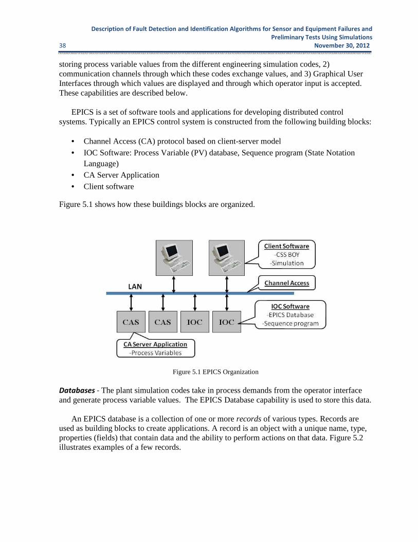
Description of Fault Detection and Identification Algorithms for Sensor and Equipment Failures and
Preliminary Tests Using Simulations 38 November 30, 2012 storing process variable values from the different engineering simulation codes, 2) communication channels through which these codes exchange values, and 3) Graphical User Interfaces through which values are displayed and through which operator input is accepted. These capabilities are described below.
EPICS is a set of software tools and applications for developing distributed control systems. Typically an EPICS control system is constructed from the following building blocks:
• Channel Access (CA) protocol based on client-server model
• IOC Software: Process Variable (PV) database, Sequence program (State Notation Language)
• CA Server Application
• Client software
Figure 5.1 shows how these buildings blocks are organized.
Figure 5.1 EPICS Organization
Databases - The plant simulation codes take in process demands from the operator interface and generate process variable values. The EPICS Database capability is used to store this data.
An EPICS database is a collection of one or more records of various types. Records are used as building blocks to create applications. A record is an object with a unique name, type, properties (fields) that contain data and the ability to perform actions on that data. Figure 5.2 illustrates examples of a few records.

Description of Fault Detection and Identification Algorithms for Sensor and Equipment Failures and
Preliminary Tests Using Simulations
November 30, 2012
ANL/NE-12/57 39
Analog input record Calculation record Binary output record
record(ai, “scs:flow") { field(DTYP,“XY566") field(SCAN,“Passive") field(EGU,"lpm") }
record(calc, "scs:alarm") { field(SCAN,“Passive") field(INPA,"scs:flow PP NMS") field(CALC,"A>10.0?1:0") }
record(bo, "scs:solenoid") { field(DTYP,“XY220") field(SCAN,“.1 second") field(OMSL,“closed_loop") field(DOL,” scs:alarm" }
Figure 5.2 Examples of EPICS Records A record performs action when it is processed. For example, when an output record is processed, it fetches the value which it is to output, converts the value, and then writes that value to the specified location. Scanning determines when a record is processed. Each record must specify the scanning method that determines when it will be processed. There are three scanning methods for database records: (1) periodic, (2) event, and (3) passive.
Communication Channels - Process variable values and control system signals are passed between plant simulation codes and databases through EPICS communication channels. A typical implementation for managing this data passing is the Input Output Controller (IOC). The IOC is a computer running software called “IOC Core”. The major software components of an IOC are depicted in Figure 5.3.
Figure 5.3. Structure of IOC
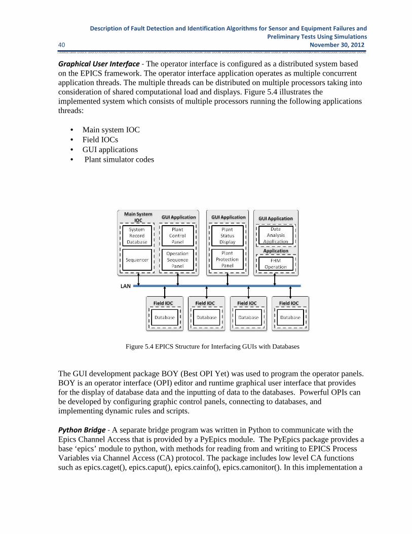
Description of Fault Detection and Identification Algorithms for Sensor and Equipment Failures and
Preliminary Tests Using Simulations 40 November 30, 2012
Graphical User Interface - The operator interface is configured as a distributed system based on the EPICS framework. The operator interface application operates as multiple concurrent application threads. The multiple threads can be distributed on multiple processors taking into consideration of shared computational load and displays. Figure 5.4 illustrates the implemented system which consists of multiple processors running the following applications threads:
• Main system IOC • Field IOCs • GUI applications • Plant simulator codes
Figure 5.4 EPICS Structure for Interfacing GUIs with Databases The GUI development package BOY (Best OPI Yet) was used to program the operator panels. BOY is an operator interface (OPI) editor and runtime graphical user interface that provides for the display of database data and the inputting of data to the databases. Powerful OPIs can be developed by configuring graphic control panels, connecting to databases, and implementing dynamic rules and scripts. Python Bridge - A separate bridge program was written in Python to communicate with the Epics Channel Access that is provided by a PyEpics module. The PyEpics package provides a base ‘epics’ module to python, with methods for reading from and writing to EPICS Process Variables via Channel Access (CA) protocol. The package includes low level CA functions such as epics.caget(), epics.caput(), epics.cainfo(), epics.camonitor(). In this implementation a
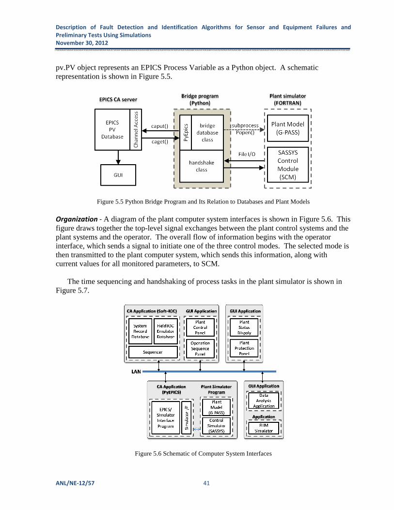
Description of Fault Detection and Identification Algorithms for Sensor and Equipment Failures and
Preliminary Tests Using Simulations
November 30, 2012
ANL/NE-12/57 41
pv.PV object represents an EPICS Process Variable as a Python object. A schematic representation is shown in Figure 5.5.
Figure 5.5 Python Bridge Program and Its Relation to Databases and Plant Models Organization - A diagram of the plant computer system interfaces is shown in Figure 5.6. This figure draws together the top-level signal exchanges between the plant control systems and the plant systems and the operator. The overall flow of information begins with the operator interface, which sends a signal to initiate one of the three control modes. The selected mode is then transmitted to the plant computer system, which sends this information, along with current values for all monitored parameters, to SCM.
The time sequencing and handshaking of process tasks in the plant simulator is shown in Figure 5.7.
Figure 5.6 Schematic of Computer System Interfaces

Description of Fault Detection and Identification Algorithms for Sensor and Equipment Failures and
Preliminary Tests Using Simulations 42 November 30, 2012
Figure 5.7 Time Sequencing and Handshaking of Tasks in Plant Simulator Hardware - The platform hardware consists of the following components:
• Four 46-inch (diagonal) flat panels.
• Dell Extreme Core I7 Studio XPS
• NVIDIA GTX460 graphics card (2)
5.2 Modules
The section describes the various modules for simulating plant processes and for executing signal processing algorithms that run under EPICS.
5.2.1 Plant
Plant simulation software is used to achieve a whole-plant simulation capability. In general the platform architecture developed under EPICS can support any plant systems code. In its present stage of development the platform provides a whole-plant simulation capability

Description of Fault Detection and Identification Algorithms for Sensor and Equipment Failures and
Preliminary Tests Using Simulations
November 30, 2012
ANL/NE-12/57 43
for reactors under the ARC and aSMR programs. These plants are liquid-metal reactor concepts with a Rankine or Brayton cycle balance of plant.
The platform is presently configured to simulate a sodium fast reactor with a super-critical carbon dioxide Brayton cycle balance of plant. The primary and intermediate system of the plant is modeled using the SASSYS one-dimensional systems code [17]. The reactor design simulated (as supplied through the SASSYS input deck) is the ABTR from [18]. The primary system of this liquid-metal reactor is configured in a pool-type arrangement with the reactor core, primary pumps, intermediate heat exchangers, and direct reactor auxiliary cooling system heat exchangers all immersed in a pool of sodium within the reactor vessel. The hot primary sodium transfers it heat to an intermediate heat exchanger. The balance of plant is modeled using the G-PASS code one-dimensional systems. The balance of plant presently simulated (as supplied through the G-PASS input deck) is the split-flow supercritical carbon-dioxide Brayton cycle. The intermediate (non-radioactive) system sodium exits the intermediate heat exchanger and flows to a Na-to-CO2 heat exchanger. This heat exchanger is the interface between the nuclear heat supply system and the Brayton cycle power conversion system. The intermediate sodium heats the supercritical CO2 which then flows into the turbine-generator performing work and generating electricity. The CO2 then goes through a series of recuperator heat exchangers, coolers, and compressors before it re-enters the Na-to-CO2 heat exchanger.
5.2.2 Control and Protection Systems
The control and protection systems are modeled using the SCM code. SCM provides for the modeling of control circuits and protection logic through a user-defined assemblage of code-provided mathematical primitives. The control systems presently simulated (as supplied through the SCM input deck) are a Generator Power Controller that uses turbine bypass and mass inventory operating in a mixed-mode and a Precooler Temperature Controller. The plant protection system is not modeled in the current SCM input deck.
Both of the controllers operate on the principle of proportional-integral (PI) control. In the general framework of the PI controller, the value of the variable ���� is forced to approach its target value ����� by repeatedly changing the value of the variable����, which has some causal relationship to����. The PI controller is described by the following set of equations forming a closed loop:
��� � ���� � ����� (5.1)
����� � �� ��� � ��� � ������
� (5.2)
��� � d�� � ���� � ����� (5.3)
Here the change ����� in the variable ���� consists of the sum of the terms proportional to the time-dependent error ��� with proportional gain constant ��, and a term proportional to the

Description of Fault Detection and Identification Algorithms for Sensor and Equipment Failures and
Preliminary Tests Using Simulations 44 November 30, 2012 integral of with integral proportional gain . These equations are represented schematically in Figure 5.8.
Figure 5.8 Schematic of a Proportional-Integral-Derivative Controller The representation of a PI controller achieved using SCM is shown in the block diagram of Figure 5.9. The individual blocks represent mathematical primitives available to the user through SCM.
Figure 5.9. SCM Block Diagram of a PI Controller The present SCM input deck is configured to force the control variables in G-PASS that drive the plant simulation. At each G-PASS time step, the SCM input deck makes available current values of the control variables from the G-PASS code, calculates the new values, and passes them back to G-PASS. Using the updated values of the control variables, G-PASS calculates the solution for the plant.
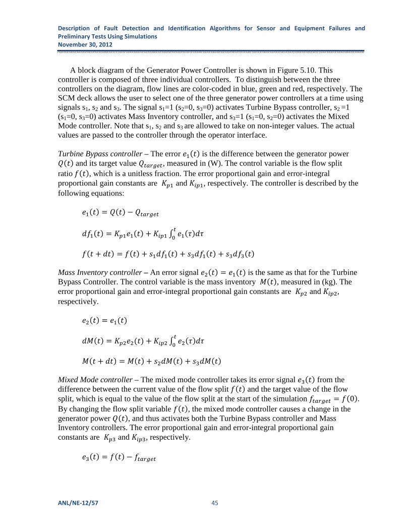
Description of Fault Detection and Identification Algorithms for Sensor and Equipment Failures and
Preliminary Tests Using Simulations
November 30, 2012
ANL/NE-12/57 45
A block diagram of the Generator Power Controller is shown in Figure 5.10. This controller is composed of three individual controllers. To distinguish between the three controllers on the diagram, flow lines are color-coded in blue, green and red, respectively. The SCM deck allows the user to select one of the three generator power controllers at a time using signals s1, s2 and s3. The signal s1=1 (s2=0, s3=0) activates Turbine Bypass controller, s2 =1 (s1=0, s3=0) activates Mass Inventory controller, and s3=1 (s1=0, s2=0) activates the Mixed Mode controller. Note that s1, s2 and s3 are allowed to take on non-integer values. The actual values are passed to the controller through the operator interface. Turbine Bypass controller – The error ���� is the difference between the generator power ���� and its target value �����, measured in (W). The control variable is the flow split ratio����, which is a unitless fraction. The error proportional gain and error-integral proportional gain constants are ��� and ����, respectively. The controller is described by the following equations:
���� � ���� � �����
������ � ��� ���� � ���� � �������
�
��� � ��� � ���� � �������� � �������� � ��������
Mass Inventory controller – An error signal ���� � ���� is the same as that for the Turbine Bypass Controller. The control variable is the mass inventory ���, measured in (kg). The error proportional gain and error-integral proportional gain constants are ��� and ����, respectively.
���� � ����
� ��� � ��� ���� � ���� � �������
�
�� � ��� � ��� � ��� ��� � ��� ���
Mixed Mode controller – The mixed mode controller takes its error signal ���� from the difference between the current value of the flow split ���� and the target value of the flow split, which is equal to the value of the flow split at the start of the simulation ����� � ��0�. By changing the flow split variable ����, the mixed mode controller causes a change in the generator power ����, and thus activates both the Turbine Bypass controller and Mass Inventory controllers. The error proportional gain and error-integral proportional gain constants are ��� and ����, respectively.
���� � ���� � �����

Description of Fault Detection and Identification Algorithms for Sensor and Equipment Failures and
Preliminary Tests Using Simulations 46 November 30, 2012
Figure 5.10. Representation of the SCM Generator Power Controller. Wiith Bpass, Inventory, and Mixed Controller Elements Differentiated by Color.
A block diagram of the Precooler Temperature PI controller is shown in Figure 5.11.
Figure 5.11 Block Diagram of Precooler Temperature PI Controller.
5.2.3 Signal Processing Routines
A capability is provided for executing signal processing routines in tandem with a plant simulation as it marches through time. The passing of data between signal processing algorithms and the plant and control system simulation codes is implemented using the EPICS channel provides protocol. The signal processing routines are run under MATLAB. The

Description of Fault Detection and Identification Algorithms for Sensor and Equipment Failures and
Preliminary Tests Using Simulations
November 30, 2012
ANL/NE-12/57 47
proper synchronization of signal processing script execution and the simulation software execution is controlled from EPICS. The entire process is represented schematically in Figure 5.12.
Figure 5.12 Signal Processing Algorithm Execution under EPICS
5.3 Operating Station
The Plant Control Station shown in Figure 5.13 provides an interactive session for manually controlling plant actuators in a SASSYS-GPASS simulation synchronized to real time. The user can choose to manipulate rod reactivity, normalized primary pump torque, normalized intermediate pump torque, and generator demand power by adjusting a corresponding slider bar. The immediate effects of these changes and the response of the plant’s safety systems can be observed in real time through plots of many different reactor variables, including: reactor power, primary and intermediate flow rates, primary and intermediate pump speeds, reactor inlet and outlet temperatures, and intermediate heat exchanger inlet and outlet temperatures. The Real Time Status Station shown in Figure 5.14 displays the instantaneous values of plant process variables against a schematic of the plant. All of the major plant components are displayed on the screen. Temperatures of various components are updated as they are calculated in real time. A blinking effect also highlights these reactor components in red when a relevant reactor variable is modified. This station allows the operator to control the balance-of-plant using one of the three control modes described earlier: bypass control, inventory control, and mixed-mode control. When an electric power change is initiated under one of these control modes, the activated valves and piping blink to show how control is being affected. This panel also provides clickable tabs at the inlet and outlet of each component. When clicked a table appears with the values of process variables.
MATLAB engine
Signal
Processing
Algorithm
Matlab
Channel
Access
(MCA)
Return Results
Train / Monitor
Get / Put
EPICS
database of
Process
Variables
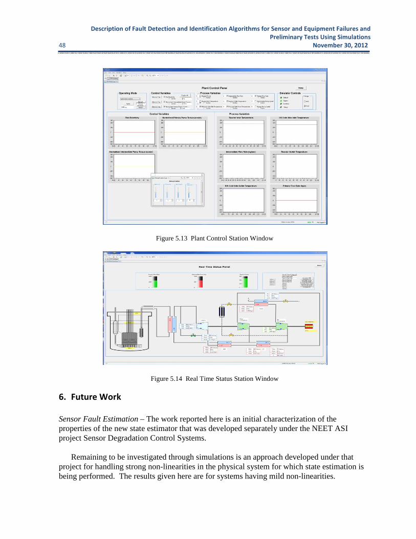
Description of Fault Detection and Identification Algorithms for Sensor and Equipment Failures and
Preliminary Tests Using Simulations 48 November 30, 2012
Figure 5.13 Plant Control Station Window
Figure 5.14 Real Time Status Station Window
6. Future Work
Sensor Fault Estimation – The work reported here is an initial characterization of the properties of the new state estimator that was developed separately under the NEET ASI project Sensor Degradation Control Systems.
Remaining to be investigated through simulations is an approach developed under that project for handling strong non-linearities in the physical system for which state estimation is being performed. The results given here are for systems having mild non-linearities.

Description of Fault Detection and Identification Algorithms for Sensor and Equipment Failures and
Preliminary Tests Using Simulations
November 30, 2012
ANL/NE-12/57 49
In principle even strong non-linearities should not present a difficulty. The methods of the above project anticipate them. However, there is some uncertainty as to how noise on the sensor readings will propagate through the algorithms of the methods. For systems exhibiting strong non-linearities operating points will be nearer than otherwise possibly creating difficulties in obtaining a good approximation for a quantity that is the analog of a derivative that is evaluated by a numerical difference. Numerical simulations are needed to assess this. Component Fault Identification – A goal for FY13 is to have a beta version of PRODIAG programmed in the new language (i.e. JBoss Drool) in an object-oriented program structure. The new implementation will be judged a success if the code passes acceptances tests which essentially require that the code produce the same results for CVCS and CCW problems for which the original PRODIAG was run.
Beyond the current fiscal year there is a need to extend the rule base. Presently the code contains no confluence rules for two-phase flow conditions. These rules are needed before the code can be applied to fault diagnoses in a feed water system or steam generator. Additionally, the code needs to be extended so diagnosis can be performed under changing conditions resulting from control system actions, in particular those in response to a fault. A conclusion based on work to date is that the current PRODIAG and the under-development object-oriented version (i.e. procedural based) are not suited to accept such changes.
A new PRODIAG architecture is needed to allow for seamless addition of new rules. The present intertwining of rule evaluation and its sequencing resulting from the procedural approach make expansion of the rule base difficult. Present automated diagnosis systems have evolved to avoid this problem by writing rules in forward chaining logic and presenting a network of such rules to an essentially standalone reasoning engine. However, the research needed to undertake this task is beyond the scope of the current multi-year project plan. It is therefore proposed that this research task be taken up in collaboration with a university funded under the NEET ASI competitive funds set-aside. The principal investigator already has an existing subcontract with the Computer Science Department at the University of Illinois Urbana-Champaign. The personnel on the subcontract are eminently qualified to take on this task. Automation – The investigation of automatic control for the CVCS described in Section 4.4 will take place in FY13.
Beyond FY13 there is interest in applying enhanced automation to the loss-of-load transient. Preliminary work [16] suggests that through modification of control algorithms there is the potential to avert a reactor scram. In principle if only control system modifications were made to the exclusion of the protection system, then licensing aspects associated with this change would be minimal.

Description of Fault Detection and Identification Algorithms for Sensor and Equipment Failures and
Preliminary Tests Using Simulations 50 November 30, 2012
7. Conclusion
On-going research to develop and evaluate operator aids that can facilitate more timely response to plant faults and grid disturbances and thereby increase plant resilience was described. The work involves collaboration between Argonne National Laboratory (ANL) and Idaho National Laboratory (INL). Presently an operator’s response to these events is hampered by the need to first process a myriad of sensor data to diagnose a fault. This research described how technology advances can contribute to increased operator awareness and aid in better formulating his response to upsets. Control actions executed in a timely manner before the plant state reaches safety settings can increase plant resilience. Ready access to procedures and to planning tools that provide trends and can project ahead based on proposed control actions support this goal. Advanced automation can play a role.
Work on three elements that address these objectives was described. A new method and approach for detecting sensor degradation and substitution of the degraded sensor reading with a high-quality estimate for the value of the underlying process variable was described. A method for diagnosing from instrumented process variables the identity of an equipment failure was described. These two capabilities provide assurance that the plant condition is known providing an opportunity for application of a third element, more refined control through automation.
A technology demonstration platform to aid in the visualization of how these technologies might integrate was described. It provides an environment for simulating the linkages among algorithms for sensor fault estimation, component fault diagnosis, and advanced control with the objective of better understanding the interactions among these three component technologies.
8. References
1. R.B.VILIM, “Design to Achieve Fault Tolerance and Resilience,” project research plan, Advanced Sensors and Instrumentation, DOE NEET program, February 2012.
2. J. P. HERZOG, S. W. WEGERICH, R. M. SINGER, and K. C. GROSS, “Theoretical Basis for the Multivariate State Estimation Technique (MSET), ANL-NT-49, December 1997.
3. K. C. GROSS, personal communication, Oracle Corporation, San Diego, California, October 2012.
4. M. YOUSUF, personal communication, Exelon Nuclear, Warrenville, Illinois, September 2012.
5. R.B.VILIM, “Sensor Degradation Control Systems,” project research plan, Advanced Sensors and Instrumentation, DOE NEET program, February 2012.
6. R. B.VILIM, “Data-Driven Estimation for Dynamic Systems: Theory and Properties,” unpublished data, Argonne National Laboratory, November 2012.
7. J. REIFMAN and T.Y.C. WEI, “PRODIAG” A Process-Independent Transient Diagnostic System – I: Theoretical Concepts,” Nuclear Science and Engineering, 131, 329-347, 1999.

Description of Fault Detection and Identification Algorithms for Sensor and Equipment Failures and
Preliminary Tests Using Simulations
November 30, 2012
ANL/NE-12/57 51
8. J. DE KLEER and J. KURIEN, “Fundamentals of Model-Based Diagnosis,” Proceedings of SafeProcess03, 2003.
9. J. DE KLEER and J. BROWN, “A Qualitative Physics Based on Confluences,” Artificial Intelligence, 24, Issue 1-3, Dec, 1984.
10. J. REIFMAN and T.Y.C. WEI, “PRODIAG” A Process-Independent Transient Diagnostic System – II: Validation Test,” Nuclear Science and Engineering, 131, 348-369, 1999.
11. J. CHOI, “Survey of Recent Advances in Diagnostic Systems,” unpublished report, Argonne National Laboratory, November 2012.
12. M. CODISH, “Logic Programming with Satisfiability,” Theory and Practice of Logic Programming, Vol. 1, Issue 8, 121-128, January 2008.
13. R. KOWALSKI, VisiRule, Logic Programming Associates, London, England, 2012 14. B. FREDERIKSEN, “Applying Expert System Technology to Code Reuse with Pyke,
PyCon 2008, Chicago, IL, March 2008. 15. P. BROWNE, JBoss Drools Business Rules, PACKT Publishing, March 2009. 16. K. THOMAS, personal communication, Idaho National Laboratory, September 2012. 17. F. E. DUNN, F.G. PROHAMMER, D. P. WEBER, and R.B. VILIM, “The SASYS-1
LMFBR Systems Analysis Code,” International Topical Meeting on Fast Reactor Safety, Knoxville, Tennessee, April 21-25, 1985.
18. Y. I. CHANG, P.J. FINCK, and C. GRANDY, “Advanced Burner Test Reactor Preconceptual Design Report,” ANL-ABR-1, Argonne National Laboratory, September 2006.

Description of Fault Detection and Identification Algorithms for Sensor and Equipment Failures and
Preliminary Tests Using Simulations 52 November 30, 2012

Description of Fault
November 30, 2012
Argonne National Laboratory is a U.S. Department of Energy laboratory managed by UChicago Argonne, LLC
Nuclear Engineering Division Argonne National Laboratory
9700 South Cass Avenue, Bldg. 208
Argonne, IL 60439-4825
www.anl.gov