description of light propagation through a circular

Description of light propagation through a circular aperture using nonparaxial

vector diffraction theory

Shekhar Guha Air Force Research Laboratory, Materials and Manufacturing Directorate, Wright-Patterson

Air Force Base, Dayton, Ohio, 45433, USA [email protected]

Glen D. Gillen Air Force Research Laboratory, Materials and Manufacturing Directorate, Anteon

Corporation, Wright-Patterson Air Force Base, Dayton, Ohio, 45433, USA [email protected]

Abstract: Using nonparaxial vector diffraction theory derived using the Hertz vector formalism, integral expressions for the electric and magnetic field components of light within and beyond an apertured plane are obtained for an incident plane wave. For linearly polarized light incident on a circular aperture, the integrals for the field components and for the Poynting vector are numerically evaluated. By further two-dimensional integration of a Poynting vector component, the total transmission of a circular aperture is determined as a function of the aperture radius to wavelength ratio. The validity of using Kirchhoff boundary conditions in the aperture plane is also examined in detail.

© 2005 Optical Society of America

OCIS codes: (050.1960) Diffraction theory

References and links 1. G. R. Kirchhoff, “Zur Theorie der Lichtstrahlen,” Ann. Phys. (Leipzig) 18, 663-695 (1883). 2. A. Sommerfeld, “Zur mathematischen Theorie der Beugungsercheinungen,” Nachr. Kgl. Wiss. Gottingen 4, 338-

342 (1894). 3. Lord Rayleigh, “On the passage of waves through apertures in plane screens, and allied problems,” Philos. Mag.

43, 259-272 (1897). 4. O. Mitrofanov, M. Lee, J. W. P. Hsu, L. N. Pfeifer, K. W. West, J. D. Wynn and J. F. Federici, “Terahertz pulse

propagation through small apertures,” App. Phys. Lett. 79, 907–909 (2001). 5. B. Lu and K. Duan, “Nonparaxial propagation of vectorial Gaussian beams diffracted at a circular aperture,” Opt.

Lett 28, 2440–2442 (2003). 6. K. Duan and B. Lu, “Vectorial nonparaxial propagation equation of elliptical Gaussian beams in the presence of

a rectangular aperture,” J. Opt. Sec. Am. A 21, 1613–1620 (2004). 7. G. D. Gillen and S. Guha, “Modeling and propagation of near-field diffraction patterns: A more complete ap-

proach,” Am. J. Phys. 72, 1195–1201 (2004). 8. W. Freude and G. K. Grau, “Rayleigh-Sommerfeld and Helmholtz-Kirchhoff integrals: application to the scalar

and vectorial theory of wave propagation and diffraction,” J. Lightwave Technol. 13, 24–32, (1995). 9. J. A. Stratton and L.J. Chu, “Diffraction theory of electromagnetic waves,” Phys. Rev. 56, 99–107, (1939).

10. H. A. Bethe, “Theory of diffraction by small holes,” Phys. Rev. 66, 163–182 (1944). 11. R. K. Luneberg, Mathematical Theory of Optics (U. California Press, Berkeley, Calif., 1964). 12. G. Bekefi, “Diffraction of electromagnetic waves by an aperture in a large screen,” J. App. Phys. 24, 1123–1130

(1953).

(C) 2005 OSA 7 March 2005 / Vol. 13, No. 5 / OPTICS EXPRESS 1424#6195 - $15.00 US Received 5 January 2005; revised 18 February 2005; accepted 18 February 2005

¨

¨

mailto:[email protected]

mailto:[email protected]

13. C. L. Andrews, “Diffraction pattern in a circular aperture measured in the microwave region,” J. Appl. Phys. 21, 761–767 (1950).

14. M. J. Ehrlich, S. Silver and G. Held,“Studies of the Diffraction of Electromagnetic waves by circular apertures and complementary obstacles: the near-zone field,” J. Appl. Phys. 26, 336–345 (1955).

15. M. Born and E. Wolf Principles of Optics (Cambridge University Press, Cambridge, 2003.) 16. A. Schoch, “Betrachtungen uber das Schallfeld einer Kolbenmembran,”Akust. Z. 6, 318–326 (1941). 17. A. H. Carter and A. O. Williams, Jr., “A New Expansion for the velocity potential of a piston source,” J. Accoust.

Soc. Am. 23, 179–184 (1951). 18. M. Mansuripur, A. R. Zakharian and J. V. Moloney, “Interaction of light with subwavelength structures,” Opt.

Photonics News, 56–61 (March 2003).

1. Introduction

Even though the diffraction of light by an aperture is a fundamental phenomenon in optics and has been studied for a long time [1–3], it continues to be of modern interest [4–8]. It has been long recognized that ‘vector’ diffraction theory needs to be used to describe propagation of light in and around structures that are of the same length scale or smaller than the wavelength of light [9]. Study of diffraction of light through an aperture with a radius (a) comparable to the wavelength of light (λ ) is a challenging phenomenon to model completely, especially for the case of a/λ ranging between 0.1 and 10, which falls in between the theory of transmission of light through very small apertures (a � λ ) [4, 10] and vector diffraction theory using Kirch-hoff boundary conditions and high-frequency approximations [5, 6, 9, 11]. The high-frequency approximations and Kirchhoff boundary conditions assume that the light field in the aperture plane is known and is unperturbed by the presence of the aperture. While mathematically con-sistent and correctly predicting light distributions beyond the aperture plane, these assumptions fail to represent physical waves in the vicinity of the aperture plane and violate Maxwell’s equations.

Paraxial approximations have historically been used to reduce the mathematical complexity and the computational time required for numerical integration, albeit at the cost of limiting the regions of their validity. The finite difference time domain (FDTD) method provides an accurate description of light distributions in the vicinity of the aperture without Kirchhoff or paraxial approximations, but can become computationally time-intensive at larger distances of propagation.

In this paper we show that using modern desktop computers, detailed solutions for all the electric and magnetic field components (as well as the Poynting vector) for all points in space in the aperture plane and beyond are obtainable for a/λ ≥ 0.1, within a reasonable period of time (minutes) using vector diffraction theory but without invoking any approximations. The expressions for the field components are first obtained here as double integrals, which are valid anywhere in space within and beyond the aperture plane. Then the field components are expressed as two computationally efficient single integrals for two mutually exclusive and all-encompassing volumes of space beyond the aperture plane. Detailed two-dimensional beam profiles of the electric field and light distributions for a variety of aperture sizes and longitu-dinal distances are presented. The resulting three-dimensional plots provide a unique visual representation of diffraction phenomena, which had been historically hindered by the excessive computational time required. Significant differences are shown to exist between the Poynting vector components and the commonly used modulus square of the electric field. It is shown that the distribution of the electric field at and near the circular aperture is not circularly symmetric, in agreement with experimental results [12–14]. However, the field distributions obtained using the Kirchhoff boundary conditions are circularly symmetric showing that for any range of aper-ture to wavelength ratios, the Kirchhoff boundary conditions are invalid at and near the aperture plane. The total power transmitted through a plane parallel to the aperture plane is calculated as


¨

a function of the aperture size. For the specific case of points along the optical axis, analytical forms of the electromagnetic field components are derived.

2. Hertz vector diffraction theory (HVDT)

The electric (E) and magnetic (H) fields of an electromagnetic wave of wavelength λ and traveling in vacuum can be determined from the polarization potential [15], or Hertz vector (ΠΠΠ), through the relations

EEE k2ΠΠΠ + ∇∇∇(∇∇∇ ΠΠΠ) , (1)

and

H − k2

iωµo ∇∇∇ ××× ΠΠΠ ik

� εo

µo ∇∇∇ ××× ΠΠΠ, (2)

where the Hertz vector is a smooth and continuous function everywhere and satisfies Maxwell’s wave equation, k 2π

λ is the wave number, and εo and µo denote the vacuum permeability and permittivity constants. For the case of a plane wave which is linearly polarized (say along the x-direction) and propagating in the +z direction, all of the E and H field components can be calculated from Πx, the x-component of the Hertz vector [12], and have the following forms:

Ex k2Πx +

∂ 2Πx

∂ x2 ,

Ey ∂ 2Πx

∂ y∂ x ,

Ez ∂ 2Πx

∂ z∂ x , (3)

and

Hx 0,

Hy − k2

iωµo

∂ Πx

∂ z ik �

εo

µo

∂ Πx

∂ z ,

Hz k2

iωµo

∂ Πx

∂ y −ik �

εo

µo

∂ Πx

∂ y . (4)

From the fields given in Eqs. (3) and (4) it is straight-forward to obtain the Poynting vector, S, where

S Re(E× H∗) Re � EyH∗

z − EzH∗ y �

i+ Re � −ExH∗

z �

j + Re � ExH∗

y �

k, (5)

and i, j, k denote the unit vectors in the x, y and z directions.

2.1. Double integral forms for the field components

We assume the plane wave described above is incident on an aperture which is perfectly con-ducting, of negligible thickness, and located in the x y plane at z 0. Because the aperture is assumed to be conducting, it is required that the tangential components of the electric field and the normal components of the magnetic field vanish in the plane of the aperture. Applying these boundary conditions on the electromagnetic fields and requiring that the Hertz vector and the


= ·

= =

=

=

=

=

=

= =

= =

=

=

- =

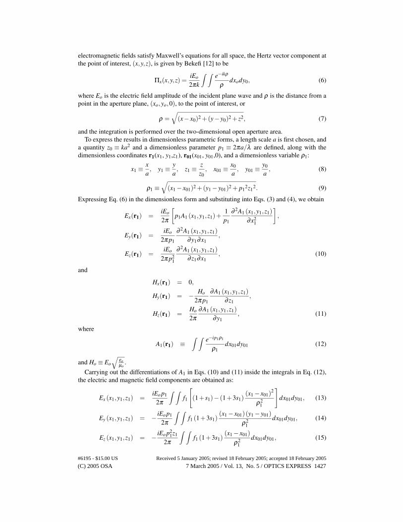
electromagnetic fields satisfy Maxwell’s equations for all space, the Hertz vector component at the point of interest, (x,y,z), is given by Bekefi [12] to be

Πx(x,y,z) = iEo

2πk

� � e−ikρ

ρ dxody0, (6)

where Eo is the electric field amplitude of the incident plane wave and ρ is the distance from a point in the aperture plane, (xo, yo,0), to the point of interest, or

ρ �

(x− x0)2 + (y− y0)2 + z2 , (7)

and the integration is performed over the two-dimensional open aperture area. To express the results in dimensionless parametric forms, a length scale a is first chosen, and

a quantity z0 ≡ ka2 and a dimensionless parameter p1 ≡ 2πa/λ are defined, along with the dimensionless coordinates r1(x1, y1,z1), r01(x01, y01,0), and a dimensionless variable ρ1:

x1 ≡ x a , y1 ≡

y a , z1 ≡

z z0

, x01 ≡ x0

a , y01 ≡

y0

a , (8)

ρ1 ≡ �

(x1− x01)2 + (y1− y01)2 + p12z12 . (9)

Expressing Eq. (6) in the dimensionless form and substituting into Eqs. (3) and (4), we obtain

Ex(r1) iEo

2π

�

p1A1 (x1,y1,z1) + 1 p1

∂ 2A1 (x1, y1,z1) ∂ x2

1

�

,

Ey(r1) iEo

2π p1

∂ 2A1 (x1,y1,z1) ∂ y1∂ x1

,

Ez(r1) iEo

2π p2 1

∂ 2A1 (x1,y1,z1) ∂ z1∂ x1

, (10)

and

Hx(r1) 0,

Hy(r1) − Ho

2π p1

∂ A1 (x1,y1,z1) ∂ z1

,

Hz(r1) Ho

2π ∂ A1 (x1,y1,z1)

∂ y1 , (11)

where

A1(r1) ≡ � � e−ip1ρ1

ρ1 dx01dy01 (12)

and Ho ≡ Eo

� εo µo

. Carrying out the differentiations of A1 in Eqs. (10) and (11) inside the integrals in Eq. (12),

the electric and magnetic field components are obtained as:

Ex (x1,y1,z1) iEo p1

2π

� � f1

�

(1+ s1) − (1+ 3s1) (x1− x01)

2

ρ2 1

�

dx01dy01, (13)

Ey (x1,y1,z1) − iEo p1

2π

� � f1 (1+ 3s1)

(x1− x01) (y1− y01) ρ2

1 dx01dy01, (14)

Ez (x1,y1,z1) − iEo p2

1z1

2π

� � f1 (1+ 3s1)

(x1− x01) ρ2

1 dx01dy01, (15)


=

=

=

=

=

=

=

=

=

=

Hx (x1,y1,z1) 0, (16)

Hy (x1,y1,z1) − Ho p3

1z1

2π

� � f1s1dx01dy01, (17)

Hz (x1,y1,z1) Ho p2

1 2π

� � f1s1 (y1− y01)dx01dy01, (18)

where

f1 ≡ e−ip1ρ1

ρ1 (19)

and

s1 ≡ 1

ip1ρ1

�

1+ 1

ip1ρ1

�

. (20)

For a circular aperture of radius a, the limits of the integrals in Eqs. (13)–(18) are: � 1

−1

� √ 1−y2

01

− √

1−y2 01

dx01dy01. (21)

2.2. Single integral forms for the field components

2.2.1. Within the geometrically illuminated region (r1 < 1)

Although the double integral forms for the electric and magnetic fields presented in the previ-ous section give the complete solution to the Hertz vector diffraction theory for any point in space with z1 ≥ 0, and can be numerically evaluated in minutes on currently available desktop computers, to obtain a detailed description of the light diffracted by the aperture over a large number of points in space, it is desirable to reduce the computation time further. Schoch [16] demonstrated that the surface integral of the Hertz vector in Eq. (6) can be expressed as a line integral around the edge of the aperture for field points within the geometrically illuminated region, or r1 < 1 where r1 is defined below in Eq. (25). Expressing Schoch’s line integral form in terms of the dimensionless parameters of Eqs. (8) and (9), the Hertz vector component for a circular aperture of radius a becomes

Πx (x1,y1,z1) = Eoa2

p2 1

�

e−ip2 1z1 −

1 2π

� 2π

0

e−ip1q

L2 (1− r1 cos φ)dφ

�

, (22)

where q2 (x1,y1,z1,φ ) = L2 + p2

1z2 1, (23)

L2 (x1, y1, φ) = 1+ r2 1− 2r1 cos φ (24)

and r1 (x1,y1) =

� x2

1 + y2 1. (25)

Substituting Eq. (22) into Eqs. (3) and (4) the electric and magnetic field components can be expressed as

Ex (x1,y1,z1) Eo

�

e−ip2 1z1 −

1 2π

� 2π

0 f2adφ

�

,

Ey (x1,y1,z1) − Eo

2π p2 1

� 2π

0 f2bdφ ,

Ez (x1,y1,z1) − Eo

2π p3 1

� 2π

0 f2cdφ , (26)


=

=

=

=

=

=

and

Hx (x1,y1,z1) 0,

Hy (x1,y1,z1) Ho

�

e−ip2 1z1 −

i 2π p2

1

� 2π

0 f2ddφ

�

,

Hz (x1,y1,z1) − iHo

2π p1

� 2π

0 f2edφ , (27)

where

f2a ≡ αβ γ + 1 p2

1 (α11β γ + β11αγ + γ11αβ ) +

2 p2

1 (α1β1γ + β1γ1α + γ1α1β ) ,

f2b ≡ α12β γ + β12αγ + γ12αβ

+α (β1γ2 + γ1β2) + β (α1γ2 + γ1α2) + γ (α1β2 + β1α2) , f2c ≡ α13β γ + α3 (β γ1 + γβ1) , f2d ≡ α3β γ,

f2e ≡ α2β γ + β2αγ + γ2αβ . (28)

The variables α , β and γ are defined as

α ≡ e−ip1q,

β ≡ 1 L2 ,

γ ≡ 1− r1 cos φ . (29)

The subscripts of α , β and γ in Eq. (28) correspond to partial derivatives; for example,

α1 ∂ α ∂ x1

, α2 ∂ α ∂ y1

, α3 ∂ α ∂ z1

,

α11 ∂ 2α

∂ x2 1

, α12 ∂ 2α

∂ y1∂ x1 , etc. (30)

The partial derivative terms of α are

α1 ≡ −ip1αq1, α2 ≡ −ip1αq2, α3 ≡ −ip1αq3, (31)

α11 ≡ −ip1 (α1q1 + αq11) , α12 ≡ −ip1 (α2q1 + αq12) , α13 ≡ −ip1 (α3q1 + αq13) , (32)

where

q1 ≡ x1δ q

, q2 ≡ y1δ q

, q3 ≡ p2

1z1

q , (33)

q11 ≡ δ q

+ x2

1 q

� cos φ

r3 1 −

δ 2

q2

�

, (34)

q12 ≡ x1y1

q

� cos φ

r3 1 −

δ 2

q2

�

, q13 ≡ −p2 1x1z1

δ q3 (35)


=

=

=

= = =

= =

and δ ≡

r1− cos φ r1

. (36)

The partial derivative terms of β are

β1 ≡ − 2L1

L3 , β2 ≡ − 2L2

L3 , (37)

β11 ≡ 6L2

1 L4 −

2L11

L3 , β12 ≡ 6L1L2

L4 − 2L12

L3 , (38)

where

L1 ≡ x1δ L

, L2 ≡ y1δ L

, (39)

L11 ≡ δ L

+ x2

1 L

� cos φ

r3 1 −

δ 2

L2

�

, L12 ≡ x1y1

L

� cos φ

r3 1 −

δ 2

L2

�

. (40)

The partial derivative terms of γ are

γ1 ≡ − x1 cos φ

r1 , γ2 ≡ −y1 cos φ

r1 , (41)

γ11 ≡ − cos φ

r1

�

1− x2

1

r2 1

�

, γ12 ≡ x1y1 cos φ

r3 1

. (42)

2.2.2. Within the geometrical shadow region (r1 > 1)

For points of interest in the geometrical shadow region, or where z1 ≥ 0 and r1 > 1, Carter and Williams [17] demonstrated that the double integral of the Hertz vector component in Eq. (6) can also be expressed as a single integral. Using the Carter and Williams’ integral form (Eq. 12 of Ref. [17]) for the double integral in Eq. (6), the Hertz vector component can be expressed as

Πx (x1,y1,z1) = a2Eo

π p2 1

� π/2

0

u v

cos ψdψ, (43)

where

u ≡ e−ip1g− e−ip1h , v ≡ �

r2 1− sin2

ψ, (44)

and

g≡ �

p2 1z2

1 + (v+ cos ψ)2 , h≡ �

p2 1z2

1 + (v− cos ψ)2 . (45)

Substituting Eq. (43) into Eqs. (3) and (4) the electric and magnetic field components become

Ex (x1,y1,z1) Eo

π

� π/2

0 f3adψ,

Ey (x1,y1,z1) Eo

π p2 1

� π/2

0 f3bdψ,

Ez (x1,y1,z1) Eo

π p3 1

� π/2

0 f3cdψ, (46)


=

=

=

and

Hx (x1,y1,z1) 0,

Hy (x1,y1,z1) iHo

π p2 1

� π/2

0 f3ddψ,

Hz (x1,y1,z1) − iHo

π p1

� π/2

0 f3edψ, (47)

where

f3a ≡ cos ψ

v

�

u+ 1 p2

1

�

u11 − 2x1u1

v2 + 3ux2

1 v4 −

u v2

��

,

f3b ≡ cos ψ

v

�

u12 − y1u1

v2 + 3x1y1u

v4 − x1u2

v2

�

,

f3c ≡ cos ψ

v

� u13 −

x1u3

v2

� ,

f3d ≡ cos ψ

v u3,

f3e ≡ cos ψ

v

� u2−

y1u v2

� . (48)

The subscripts of u correspond to partial derivatives (as in Eq. (30)):

u1 ≡ −ip1

� g1e−ip1g− h1e−ip1h

� , u2 ≡ −ip1


� , (49)

u3 ≡ −ip3 1z1

� e−ip1g

g −

e−ip1h

h

�

, (50)

u11 ≡ −ip1


� − p2

1

� g2

1e−ip1g− h2 1e−ip1h

� ,

u12 ≡ −ip1


� − p2

1

� g1g2e−ip1g− h1h2e−ip1h

� ,

u13 ≡ −ip1


� − p2

1

� g1g3e−ip1g− h1h3e−ip1h

� , (51)

where

g1 ≡ x1ga, g2 ≡ y1ga, g3 ≡ z1 p2

1 g

, (52)

g11 ≡ ga − x2

1 g

� g2

a + cos ψ

v3

� , g12 ≡ −

x1y1

g

� g2

a + cos ψ

v3

� , g13 ≡ −

x1z1 p2 1

g2 ga, (53)

h1 ≡ x1ha, h2 ≡ y1ha, h3 ≡ z1 p2

1 h

, (54)

h11 ≡ ha − x2

1 h

� h2

a − cos ψ

v3

� , h12 ≡ −

x1y1

h

� h2

a − cos ψ

v3

� , h13 ≡ −

x1z1 p2 1ha

g2 , (55)

and ga ≡

v+ cos ψ vg

, ha ≡ v− cos ψ

vh . (56)

Even though the single integral expressions for E and H (Eqs. (26), (27), (46) and (47)) involve a large number of terms, they can be evaluated significantly (10 to 15 times) faster than the double integral expressions (Eqs. (13)–(18)).


=

=

=

3. Vector diffraction theory using Kirchhoff boundary conditions (KVDT)

The Hertz vector diffraction theory (HVDT) described above provides the values of the elec-tromagnetic fields in the aperture plane and beyond. The Kirchhoff boundary conditions, on the other hand, specify the values of the fields in the aperture plane. Starting from these specified values at z 0 the fields for z > 0 can be obtained using the Green’s function method of solution of the wave equation. Luneberg [11] has shown how the Green’s function method can be used to derive the longitudinal component (Ez) of the fields from the known transverse components in the aperture plane.

Luneberg’s method has recently been used by Lu and Duan [5, 6] to derive analytical ex-pressions for the electric field components of diffracted waves beyond the aperture. However, despite the claim in Refs. [5, 6] that the treatment of the problem is nonparaxial, the analytical expressions derived there are based upon the assumption that the on-axis distance to the point of interest is large compared to the radial distance (Eq. 6 in Lu and Duan [5] and Eq. 7 in Duan and Lu [6]). Here we derive the vector components of the electric and magnetic fields in terms of double integrals in dimensionless parameters for incident planar beam distributions of arbi-trary shape, using the Kirchhoff boundary conditions, with the aim of determining the region of their validity. Neither the paraxial (Fresnel) approximation nor the approximations used by Lu and Duan [5, 6] are invoked here.

Given a beam of light whose electric field distribution in the plane z 0 is known in terms of the coordinates x0 and y0 in the plane as E Ex(r0)i + Ey(r0) j, the field at a point r xi+ y j + zk is given by [11]

Ex(r) = − 1

2π

� � ∞

−∞ Ex(r0)

∂ G(r,r0) ∂ z

dx0dy0, (57)

Ey(r) = − 1

2π

� � ∞

−∞ Ey(r0)

∂ G(r,r0) ∂ z

dx0dy0, (58)

where r0 x0 i+ y0 j. The Green’s function G used in Eqs. (57) and (58) is given by

G(r,r0) = e−ikρ

ρ , (59)

and the distance ρ is defined in Eq. (7). Using Eqs. (57) and (58) in the Maxwell equation ∇ E 0 in charge-free space, i.e.,

∂ Ez

∂ z −

� ∂ Ex

∂ x +

∂ Ey

∂ y

�

, (60)

and interchanging the orders of the partial derivatives of G, we obtain

2π ∂ Ez

∂ z

� � ∞

−∞

�

Ex(r0) ∂ 2G ∂ x∂ z

+ Ey(r0) ∂ 2G ∂ y∂ z

�

dx0dy0

∂ ∂ z

�� ∞

−∞

�

Ex(r0) ∂ G ∂ x

+ Ey(r0) ∂ G ∂ y

�

dx0dy0

�

. (61)

From Eq. (61), Ez is obtained as

Ez(r) 1

2π

� � ∞

−∞

�

Ex(r0) ∂ G ∂ x

+ Ey(r0) ∂ G ∂ y

�

dx0dy0 + F1(x,y), (62)

where F1(x,y) is a function to be determined from the boundary conditions. The term F1(x,y), was ignored in previous treatments [5, 6, 11], and is necessary for Ez to approach the imposed boundary condition as z approaches 0.


=

= = =

=

· =

=

=

=

=

Using the length scale a, the quantity z0 ≡ ka2, the dimensionless parameter p1 ≡ 2πa/λ , and the normalized units of Eqs. (8) and (9) as before, and the expression for the Green’s function from Eq. (59), the three components of the electric field vector can now be rewritten as

Ex(r1) − p3

1z1

2π

� � ∞

−∞ Ex(r01) f1s1dx01dy01,

Ey(r1) − p3

1z1

2π

� � ∞

−∞ Ey(r01) f1s1dx01dy01,

Ez(r1) p2

1 2π

�� ∞

−∞

� Ex(r01)(x1− x01)

+Ey(r01)(y1− y01) �

f1s1dx01dy01

� + F1(x1,y1), (63)

where f1 and s1 are defined in Eqs. (19) and (20). The magnetic field components can be derived similarly to the derivation of the electric field

components using Green’s theorem in Eqs. (57) - (62), yielding

Hx(r1) − p3

1z1

2π

� � ∞

−∞ Hx(r01) f1s1dx01dy01,

Hy(r1) − p3

1z1

2π

� � ∞

−∞ Hy(r01) f1s1dx01dy01,

Hz(r1) p2

1 2π

�� ∞

−∞

� Hx(r01)(x1− x01)

+ Hy(r01)(y1− y01) �

f1s1dx01dy01

� + F2(x1, y1), (64)

where F2(x1, y1) is a function to be determined from the boundary conditions. Using Eqs. (63) and (64) the Poynting vector components can be calculated from Eq. (5).

In the Kirchhoff formalism [9] the field components on the dark side of the screen are as-sumed to be zero except at the opening, where they have their undisturbed values that they would have had in the absence of the screen. For a linearly polarized plane wave light beam (say with E in the x-direction, and H in the y-direction) incident on a circular aperture of radius a in an opaque screen, the electric field components just at the exit of the aperture (at the z 0 plane) are then

Ex(x01, y01,0) �

E0 if x2 01 + y2

01 < 1 0 otherwise

Ey(x01, y01,0) 0 Ez(x01, y01,0) 0, (65)

and the magnetic field components are

Hx(x01, y01,0) 0

Hy(x01, y01,0) �

H0 if x2 01 + y2

01 < 1 0 otherwise

Hz(x01, y01,0) 0. (66)

Inserting Eqs. (65) and (66) in Eqs. (63) and (64), the expressions for the electric and mag-netic fields are obtained:

Ex(x1,y1,z1) −E0 p3

1z1

2π B1(x1,y1,z1), (67)


=

=

=

=

=

=

=

=

=

=

=

=

=

=

Ey(x1,y1,z1) 0, (68)

Ez(x1,y1,z1) E0 p2

1 2π

[B2(x1,y1,z1) − B2(x1,y1,0)] , (69)

and

Hx(x1,y1,z1) 0, (70)

Hy(x1,y1,z1) −H0 p3

1z1

2π B1(x1,y1,z1), (71)

Hz(x1,y1,z1) H0 p2

1 2π

[B3(x1, y1, z1) − B3(x1,y1,0)] , (72)

where

B1(x1,y1,z1) � 1

−1

� √ 1−y2

01

− √

1−y2 01

f1s1dx01dy01, (73)

B2(x1,y1,z1) � 1

−1

� √ 1−y2

01

− √

1−y2 01

f1s1(x1− x01)dx01dy01, (74)

B3(x1,y1,z1) � 1

−1

� √ 1−y2

01

− √

1−y2 01

f1s1(y1− y01)dx01dy01. (75)

The terms B2(x1,y1,0) and B3(x1, y1,0) in Eqs. (69) and (72) arise from the presence of the terms F1(x1,y1) and F2(x1,y1) in Eqs. (62)–(64). They ensure that the boundary conditions Ez Hz 0 at z1 0 (Eqs. (65) and (66)) are valid. As mentioned earlier, they have been ignored in Refs.[5, 6, 11], so that the calculated longitudinal field components Ez and Hz obtained there do not vanish at z1 0, contradicting the boundary condition.

It should be noted that both the Ex and Hy KVDT integrals (Eqs. (67), (71) and (73)) have the same form as the Hy HVDT double integral (Eq. (17)) and one of the four integral terms of the HVDT Ex component (Eq. (13)), and are radially symmetric with respect to x1 and y1. Therefore the calculated fields of Ex and Hy using KVDT will always have radial symmetry and are independent of the orientation of the polarization for normally incident light. In contrast, the HVDT method shows (Eqs. (13)–(18)) that the components of all the electromagnetic fields except Hx and Hy are dependent on the direction of the incident polarization.

4. Analytical on-axis expressions and calculations

4.1. Analytical on-axis expressions using HVDT

Starting with the Hertz vector diffraction theory, analytical expressions for the components of E and H for on-axis positions and z1 ≥ 0 can be obtained by direct integration. Using Eqs. (3) and (6) the on-axis integral expression for Ex can be found to be

Ex(0,0,z1) Eo i

2π

��

p1 e−ip1r2

r2 − i

e−ip1r2

r2 2

− e−ip1r2

p1r3 2 − p1x2

01 e−ip1r2

r2 2

+3ix2 01

e−ip1r2

r4 2

+ 3x2 01

e−ip1r2

p1r5 2

�

dx01dy01

�

, (76)

where r2

� x2

01 + y2 01 + p2

1z2 1. (77)


=

=

=

=

=

=

=

=

= = =

=

=

=

After converting to polar coordinates and integrating the angular terms, the radial integral is integrated by parts where the definite integral from each term in Eq. (76) cancels with that of another term’s definite integral. The resulting analytical expression for the on-axis x-component of the electric field becomes

Ex(0,0,z1) Eo i 2

�

i(e1− e2) − 1 p1

� e1

d1 −

e2

d2

�

+ip2 1z2

1

� e1

d2 1 −

e2

d2 2

�

+ p1z2 1

� e1

d3 1 −

e2

d3 2

��

, (78)

where

e1 e−ip1 √

1+p2 1z2

1 ,

e2 e−ip2 1z1 ,

d1

� 1+ p2

1z2 1,

d2 p1z1. (79)

Similarly, for on-axis points the double integral expression for the y-component of the mag-netic field becomes

Hy (0, 0,z1) = Ho p1z1

2π

� � �

ip1 e−ip1r2

r2 2

+ e−ip1r2

r3 2

�

dx01dy01, (80)

which can be integrated to

Hy (0,0, z1) = Ho

⎛ ⎝e−ip2 1z1 − p1z1

e−ip1 √

1+p2 1z2

1 � 1+ p2

1z2 1

⎞ ⎠ . (81)

Using Eqs. (78) and (81) the z-component of the Poynting vector can be evaluated for on-axis points.

At the center of the circular aperture the real and imaginary components of Ex reduce to

Real [Ex (0,0,0)] = Eo

�

1− 1 2

�

cos p1 + sin p1

p1

��

(82)

and

Imaginary [Ex (0,0,0)] = − Eo

2

� cos p1

p1 − sin p1

�

, (83)

while Hy/Ho approaches unity for all values of p1.

4.2. Analytical on-axis expressions using KVDT

For on-axis points (x1 y1 0) the non-zero components of the fields evaluated from the KVDT integral term B1 (Eq. (73)) also reduce to the analytical forms:

Ex(0,0,z1) = Eo

⎛ ⎝e−ip2 1z1 − p1z1

e−ip1 √

1+p2 1z2

1 � 1+ p2

1z2 1

⎞ ⎠ , (84)

and

Hy(0,0,z1) = Ho

⎛ ⎝e−ip2 1z1 − p1z1

e−ip1 √

1+p2 1z2

1 � 1+ p2

1z2 1

⎞ ⎠ . (85)


=

=

=

=

=

==

As z1 approaches the aperture plane, both Ex/Eo and Hy/Ho approach unity and are indepen-dent of the value of p1 and the orientation of the incident polarization.

The KVDT integrals B2 and B3 are identically equal to zero for x1 y1 0, so that the longitudinal components Ez and Hz vanish for on-axis points, and the Poynting vector only has a z-component, or

S(0,0,z1) = S0

⎛ ⎝ 1+ 2p2 1z2

1

1+ p2 1z2

1 −

2p1z1 � 1+ p2

1z2 1

cos

�

p2 1z1

��

1+ 1

p2 1z2

1 − 1

��⎞ ⎠ k, (86)

where

So ≡ EoH∗ o

� εo

µo |Eo|2 (87)

denotes the intensity of the incident undisturbed beam. Due to the cosine term in Eq. (86), the on-axis value of the Poynting vector oscillates with z1

for p1 > π , with locations of the maxima and the minima given by

z1m p2

1− m2π2

2mπ p2 1

, (88)

where m has integer values from 1 to p1/π . Odd values of m correspond to maxima and even values correspond to minima. The value of m 1 gives the location of the on-axis maximum farthest from the aperture, and is roughly 1/(2π) for large values of p1.

5. Power transmission function

The radiative power transmitted through a surface normal to the z-axis is given by

Pz (z1) �

∞

−∞

� ∞

−∞ Sz (x1,y1,z1)dx1dy1. (89)

Defining Po ≡ πa2So as the amount of unperturbed incident power that would be intercepted by the aperture, the power transmission function of the aperture, T , is given by

T ≡ Pz

Po

1 Po

� ∞

−∞

� ∞

−∞ Sz (x1,y1,z1) dx1dy1, (90)

where Sz is determined from the calculated values of E and H for a given value of a/λ .

6. Calculation of electromagnetic fields and Poynting vectors

In this section the results of the calculations of the electromagnetic field integrals are presented. The expressions derived in sections 2–5 were calculated on commonly available desktop com-puters (2.4 GHz Pentium processor) using the commercial software Mathcad. The tolerance of integration in Mathcad was typically set between 10−3 and 10−5. The calculation time required to run the single integral expressions was found to be approximately 10 to 15 times faster than that required for a calculation using the double integral expressions.

6.1. Beam distributions in the aperture plane

Figures 1–9 show the distributions of the normalized fields and normalized axial Poynting vector component, Sz/So, in the aperture plane. These results were obtained from the previously derived integral expressions by setting z1 10−5 and making sure that the values of the integrals


==

=

=

=

=

=

=

were unchanged when a smaller value of z1 was chosen. A convention adopted in the following figures is that in each graph, solid lines denote the real components and the dotted lines denote the imaginary components of the fields.

Figure 1 shows the calculation of the x-component of the electric field in the aperture plane as a function of x1 and y1, for a/λ 5. The calculated Ex field is seen to exhibit radial asym-metry in agreement with experimental measurements by Andrews [13] and Ehrlich et al. [14] in the aperture plane for diffraction of microwave radiation. The number of oscillations of Ex along the y-axis from the center of the aperture to the edge is equal to the aperture to wave-length ratio, a/λ . Along with the strong asymmetry in the x and y-directions, it is seen that the value of the real part of Ex at the center of the aperture is Eo/2, whereas according to Kirchhoff approximations, Ex should be equal to Eo everywhere in the aperture. The real and imaginary parts of Ex(0,0,0) obtained from Eqs. (82) and (83), are plotted as a function of a/λ in Figs. 2(a) and (b), respectively. Figure 2 shows that at the aperture plane, the Kirchhoff approximation is not valid even for large values of a/λ , with the real part of Ex oscillating between 0.5 and 1.5, for all a/λ > 0.5. The oscillations of Fig. 2, which continue indefinitely as p1 increases, with values of 1.5 occurring for a/λ values having half-integer values, and 0.5 for integer values, have previously been experimentally demonstrated [14]. Eq. (83) also shows that as p1, i.e. a/λ , goes to zero, the value of the imaginary part of Ex(0,0,0) diverges as 1/p1, thereby implying that the HVDT theory described here is invalid for small p1 (< 0.1.) The results presented here match the experimental measurements for a/λ ≥ 0.5 shown in Ref. [12–14]. The present HVDT results may therefore be considered to be valid for a/λ ≥ 0.5.

Figure 1 also shows that near the rim of the aperture the imaginary component of Ex increases rapidly in magnitude, causing the modulus square of the electric field to diverge as x1 → ±1. At the same positions in space however, Hy rapidly approaches zero. The resulting z-component of the Poynting vector, Sz, has a smooth and continuous transition across the rim of the aperture, unlike |Ex|2, as illustrated in Fig. 3(a). There are also significant differences between |Ex|2

and Sz in the aperture plane along the y-axis, as shown in Fig. 3(b). The values of Ex and Hy displayed in Fig. 3 were calculated using Eqs. (26) and (27) for r1 < 1 and Eqs. (46) and (47) for r1 > 1. Other electromagnetic field components (Ey, Ez and Hz) also possess some structure in the aperture plane, but with negligible (< 10−3) magnitudes.

The expression of the Hertz vector integrals in the single integral forms allow detailed cal-culations of the light intensity distribution in the aperture plane (as well as beyond it) as shown in Figs. 4–9. To obtain adequate resolution in these two-dimensional plots, 200 by 200 single integrals were calculated for each quadrant which took approximately four hours to run. Cal-culation of the intensity values over an array of the same size using the double integrals took approximately 60 hours.

To emphasize the difference between the squared modulus of the electric field, |Ex|2, and the Poynting vector component, Sz, the two-dimensional distribution of |Ex/Eo|2 and Sz/So are plotted in Figs. 4 and 5, respectively, both for a/λ 5. As mentioned before, even in the aperture plane, the transition of the Poynting vector component Sz between the illuminated and the dark region is smooth, whereas according to the Kirchhoff boundary conditions, there is a sharp discontinuity of the electric field (as well as Sz) at the boundary.

In Figs. 6–9, the x y distribution of Sz in the aperture plane is plotted for a/λ 2.5, 2, 1, and 0.5, respectively. From the center of the aperture out to the rim along the y-axis, the number of oscillations of Sz equals the value of a/λ . Figure 9 illustrates that for a/λ < 1 the oscillatory behavior of Ex, and subsequently Sz, in the aperture plane have been eliminated, and an ellipticity in the beam profile has become the dominant characteristic.


=

=

- =

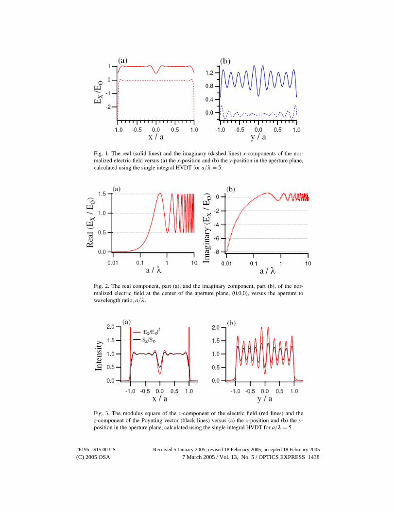
Fig. 1. The real (solid lines) and the imaginary (dashed lines) x-components of the nor-malized electric field versus (a) the x-position and (b) the y-position in the aperture plane, calculated using the single integral HVDT for a/λ 5.

Fig. 2. The real component, part (a), and the imaginary component, part (b), of the nor-malized electric field at the center of the aperture plane, (0,0,0), versus the aperture to wavelength ratio, a/λ .

Fig. 3. The modulus square of the x-component of the electric field (red lines) and the z-component of the Poynting vector (black lines) versus (a) the x-position and (b) the yposition in the aperture plane, calculated using the single integral HVDT for a/λ 5.


=

-=

Fig. 4. Calculated modulus square of the x-component of the electric field (|Ex/Eo|2) versus x and y in the aperture plane using single integral HVDT,

� (x/a)2 + (y/a)2 < 1 and for

a/λ 5.

6.2. Beam distributions beyond the aperture plane

6.2.1. On-axis calculations

The analytical expressions obtained for the fields for on-axis points, (x y 0), in Eqs. (78), (81), (84) and (85) provide an understanding of the behavior of the beam away from the aperture plane. In Fig. 10 the on-axis values of Sz/So calculated using HVDT (Eqs. (78) and (81)) and KVDT (Eqs. (84) and (85)) are plotted along with the on-axis value of |Ex/Eo|2

(from Eq. (78)) for a/λ 0.5, 1, 2.5 and 5. As discussed before, for a/λ > 1 the on-axis in-tensity values go through a number of minima and maxima, with the total number of minima or maxima roughly equal to the value of a/λ and the positions of the maxima or minima given by z1 ≈ 1/(2mπ) where the maxima occur for odd integer values of m and the minima occur for even integer values of m. The last maximum (farthest from the aperture) occurs at z1 ≈ 1/(2π), and for z1 ≥ 1/(2π) the intensity drops off as 1/z2

1, corresponding to the spreading of a spherical wave.

For small z1, i.e., in and near the aperture plane, the HVDT and KVDT results are different from each other and from |Ex/Eo|2 for all the cases of a/λ , as shown in Fig. 10. However, the HVDT and KVDT results and |Ex/Eo|2 come close to each other, even for a/λ 0.5, for z1 > 0.2. This implies that even for a/λ ≈ 0.5, KVDT can be used to predict beam shapes at planes sufficiently far away from the aperture.


=

= =

=

=

Fig. 5. Calculated z-component of the Poynting vector (Sz/So) versus x and y in the aperture plane using single integral HVDT,

� (x/a)2 + (y/a)2 < 1 and for a/λ 5.


� (x/a)2 + (y/a)2 < 1 and for a/λ 2.5.


=

=


� (x/a)2 + (y/a)2 < 1 and for a/λ 2.


� (x/a)2 + (y/a)2 < 1 and for a/λ 1.


=

=


� (x/a)2 + (y/a)2 < 1 and for a/λ 0.5.

6.2.2. Diffracted beam shapes

To determine if the radial asymmetry observed for a/λ 0.5 in Fig. 9 persists as the beam propagates away from the aperture, the dependence of Sz/So on the radial coordinate r1 is plotted along the x and y axes in Figs. 11(a)–(c) for a/λ 0.5 and in Figs. 11(d)–(f) for a/λ 5 for three different values of z1 (10−4, 0.1 and 1). Figure 11(a)–(c) shows that for a/λ 0.5, at the aperture plane (z1 10−4) the beam is elliptically shaped with the major axis in the xdirection. Results of calculation using the FDTD method (for a/λ 0.308, at z1 0.052) are shown in Ref. [18]. The plot of transmitted intensity “corresponding to Ex” in Fig. 10 of [18] also shows the radial asymmetry and the elongation of the beam along the x-axis. As the beam propagates, the ellipticity decreases and beyond z1 > 0.1 the beam becomes elongated along the y-axis. The plots in Figs. 11(d)–(f) show that for larger a/λ values, although the beam is strongly asymmetric near the aperture plane, as it propagates away from the aperture plane it becomes radially symmetric more quickly than for the smaller a/λ case. Figures 12 and 13 show the detailed two-dimensional distribution of Sz/So at the positions of an axial maximum (z1 1/(6π)) and an axial minimum (z1 1/(4π)), for a/λ 5.

6.3. The longitudinal component of the electric field: Ez

Along with the transverse field components, the Hertz vector theory allows the calculation of the longitudinal fields Ez and Hz as well. Since the incident unperturbed light beam is assumed to be a plane wave, it has no longitudinal field components. According to Eqs. 6c and 8 in Ref. [12], Ez vanishes within the aperture at the aperture plane. Evaluation of the integral in Eq. (15) at various x1, y1 points within the aperture shows that the integral is independent of z1 as z1 approaches 0, so that Ez is proportional to z1. This verifies that (consistent with the


=

=

= = =

= = =

= = =

Fig. 10. Calculated on-axis values for the modulus square of the x-component of the electric field (red line) using HVDT, the z-component of the Poynting vector (black line) using HVDT, and the z-component of the Poynting vector (blue line) using KVDT for: (a) a/λ 0.5, (b) a/λ 1, (c) a/λ 2.5 and (d) a/λ 5.

Fig. 11. Calculated Sz/So for a/λ 0.5 with (a) z1 10−4, (b) z1 0.1, (c) z1 1, and for a/λ 5 with (d) z1 10−4, (e) z1 0.1, and (f) z1 1, using the single integral HVDT. The distance r1 is either x or y normalized to the aperture radius, a.


= = = =

= = = = = = = =

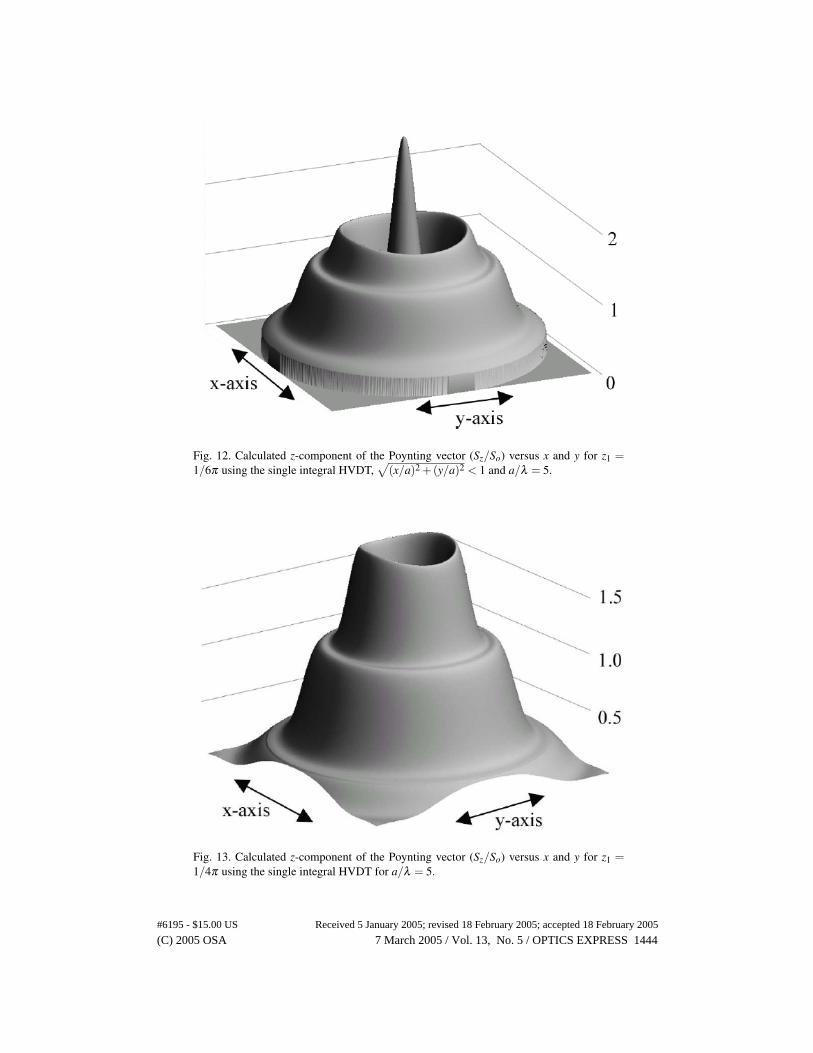
Fig. 12. Calculated z-component of the Poynting vector (Sz/So) versus x and y for z1 1/6π using the single integral HVDT,

� (x/a)2 + (y/a)2 < 1 and a/λ 5.

Fig. 13. Calculated z-component of the Poynting vector (Sz/So) versus x and y for z1 1/4π using the single integral HVDT for a/λ 5.


= =

= =

Fig. 14. Calculated real, (a), and imaginary, (b), components of Ez/Eo for θ 0◦ (x-axis), 22.5◦, 45◦, 67.5◦ and 90◦ (y-axis), for a/λ 0.5 and z1 0.05.

Fig. 15. Calculated real, (a), and imaginary, (b), components of Ez/Eo for θ 0◦ (x-axis), 22.5◦, 45◦, 67.5◦ and 90◦ (y-axis), for a/λ 5 and z1 0.05.

requirement of Maxwell’s equations) Ez vanishes in the aperture plane, i.e., when z1 → 0. Here we present the results of some calculations showing distribution of Ez/Eo at various distances near the aperture. Figures 14 and 15 show the dependence of Ez/Eo on the radial coordinate r1 for various values of the angular coordinate θ , for a/λ 0.5 and 5 respectively, at a distance of z1 0.05. It is seen that the maximum value of both the real and the imaginary parts of Ez/Eo (for both values of a/λ ) are obtained for θ1 0, i.e., along the x-axis. Figures 16 and 17 show the dependence of Ez/Eo on x1 (for y1 0) at various distances from the aperture (z1 0.05, 0.1, 0.5, and 1) for a/λ 0.5 and 5, respectively. It is seen that even for a/λ 5, the Ez can be a substantial fraction (20 percent) of the incident field amplitude at certain positions in front of the aperture.

6.4. Power transmission function calculations

Evaluating T using Eq. (90) for different z1 values shows that for fields calculated using HVDT, T is independent of z1. In contrast, if the fields calculated using KVDT are used to calculate Pz, the value of T depends upon z1, thus showing that the Kirchhoff assumption is in violation of the conservation of energy principle as well as of the Maxwell’s equations.


= = =

= = =

= =

= = =

= =

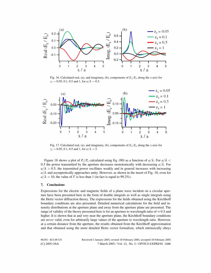
Fig. 16. Calculated real, (a), and imaginary, (b), components of Ez/Eo along the x-axis for z1 0.05, 0.1, 0.5 and 1, for a/λ 0.5.

Fig. 17. Calculated real, (a), and imaginary, (b), components of Ez/Eo along the x-axis for z1 0.05, 0.1, 0.5 and 1, for a/λ 5.

Figure 18 shows a plot of Pz/Po calculated using Eq. (90) as a function of a/λ . For a/λ < 0.5 the power transmitted by the aperture decreases monotonically with decreasing a/λ . For a/λ > 0.5, the transmitted power oscillates weakly and in general increases with increasing a/λ and asymptotically approaches unity. However, as shown in the insert of Fig. 18, even for a/λ 10, the value of T is less than 1 (in fact is equal to 99.2%).

7. Conclusions

Expressions for the electric and magnetic fields of a plane wave incident on a circular aper-ture have been presented here in the form of double integrals as well as single integrals using the Hertz vector diffraction theory. The expressions for the fields obtained using the Kirchhoff boundary conditions are also presented. Detailed numerical calculations for the field and in-tensity distributions at the aperture plane and away from the aperture plane are presented. The range of validity of the theory presented here is for an aperture to wavelength ratio of ≈ 0.5 and higher. It is shown that at and very near the aperture plane, the Kirchhoff boundary conditions are never valid, even for arbitrarily large values of the aperture to wavelength ratio. However, at a certain distance from the aperture, the results obtained from the Kirchhoff approximation and that obtained using the more detailed Hertz vector formalism, which intrinsically obeys


= =

= =

=

Fig. 18. Calculated transmission function as a function of the aperture radius to wavelength of light ratio, calculated using HVDT.

Maxwell’s equations, are about identical, even for aperture to wavelength ratios as small as 0.5. Radial asymmetry of the electric field distribution for small circular apertures have been experimentally demonstrated before. Here we have presented, for the first time to our knowl-edge, calculations of the detailed two-dimensional field and intensity distributions, along with the calculation of the longitudinal component (Ez) of the electric field using the Hertz vector diffraction theory.

Schoch [16] has shown that the double integral of Πx in Eq. (6) over a surface can be trans-formed into a line integral along the aperture edge for an aperture of arbitrary shape. The method described here for a circular aperture can therefore be extended to elliptical or rec-tangular apertures.

Acknowledgment

The authors thank Prof. Wolfgang Freude of Universitat Karlsruhe for pointing out to them the limitations of the Kirchhoff boundary conditions at the Annual Meeting of the Optical Society of America, Rochester, New York, October 2004.


description of light propagation through a circular

Documents