descriptive discriminant analysis for repeated measures data

Descriptive Discriminant Analysis for Repeated Measures Data

A Dissertation Submitted to the College of

Graduate Studies and Research

in Partial Fulfillment of the Requirements

for the Degree of Doctor of Philosophy

in the Collaborative Graduate Program in Biostatistics

University of Saskatchewan

Saskatoon

By

Tolulope Timothy Sajobi

© Copyright Tolulope Timothy Sajobi, 2012. All rights reserved

i

Permission to Use

In presenting this dissertation in partial fulfillment of the requirements for a Postgraduate

degree from the University of Saskatchewan, I agree that the Libraries of this University may

make it freely available for inspection. I further agree that permission for copying of this

thesis/dissertation in any manner, in whole or in part, for scholarly purposes may be granted

by the professor or professors who supervised my thesis/dissertation work or, in their

absence, by the Head of the Department or the Dean of the College in which my thesis work

was done. It is understood that any copying or publication or use of this thesis/dissertation or

parts thereof for financial gain shall not be allowed without my written permission. It is also

understood that due recognition shall be given to me and to the University of Saskatchewan

in any scholarly use which may be made of any material in my thesis/dissertation.

Requests for permission to copy or to make other uses of materials in this dissertation

in whole or part should be addressed to:

Graduate Chair, Collaborative Biostatistics Program

School of Public Health

University of Saskatchewan

107 Wiggins Road

Saskatoon, Saskatchewan

S7N 5E5 Canada

ii

Abstract

Background: Linear discriminant analysis (DA) encompasses procedures for classifying

observations into groups (predictive discriminant analysis, PDA) and describing the relative

importance of variables for distinguishing between groups (descriptive discriminant analysis,

DDA) in multivariate data. In recent years, there has been increased interest in DA

procedures for repeated measures data. PDA procedures that assume parsimonious repeated

measures mean and covariance structures have been developed, but corresponding DDA

procedures have not been proposed. Most DA procedures for repeated measures data rest on

the assumption of multivariate normality, which may not be satisfied in biostatistical

applications. For example, health-related quality of life (HRQOL) measures, which are

increasingly being used as outcomes in clinical trials and cohort studies, are likely to exhibit

skewed or heavy-tailed distributions. As well, measures of relative importance based on

discriminant function coefficients (DFCs) for DDA procedures have not been proposed for

repeated measures data. Purpose: The purpose of this research is to develop repeated

measures discriminant analysis (RMDA) procedures based on parsimonious covariance

structures, including compound symmetric and first order autoregressive structures, and that

are robust (i.e., insensitive) to multivariate non-normal distributions. It also extends these

methods to evaluate the relative importance of variables in multivariate repeated measures

(i.e., doubly multivariate) data. Method: Monte Carlo studies were conducted to investigate

the performance of the proposed RMDA procedures under various degrees of group mean

separation, repeated measures correlation structures, departure from multivariate normality,

and magnitude of covariance mis-specification. Data from the Manitoba Inflammatory Bowel

Disease Cohort Study, a prospective longitudinal cohort study about the psychosocial

iii

determinants of health and well-being, are used to illustrate their applications. Results: The

conventional maximum likelihood (ML) estimates of DFCs for RMDA procedures based on

parsimonious covariance structures exhibited substantial bias and error when the covariance

structure was mis-specified or when the data followed a multivariate skewed or heavy-tailed

distribution. The DFCs of RMDA procedures based on robust estimators obtained from

coordinatewise trimmed means and Winsorized variances, were less biased and more

efficient when the data followed a multivariate non-normal distribution, but were sensitive to

the effects of covariance mis-specification. Measures of relative importance for doubly

multivariate data based on linear combinations of the within-variable DFCs resulted in the

highest proportion of correctly ranked variables. Conclusions: DA procedures based on

parsimonious covariance structures and robust estimators will produce unbiased and efficient

estimates of variable relative importance of variables in repeated measures data and can be

used to test for change in relative importance over time. The choice among these RMDA

procedures should be guided by preliminary descriptive assessments of the data.

iv

Acknowledgements

My profound gratitude goes to my PhD advisor, Dr. Lisa Lix, who has mentored me

in research, critical thinking, and scientific writing. I am indebted to her invaluable insight,

suggestion for improvements, and motivation during the program. I also thank members of

my Advisory Committee for their invaluable contributions, suggestions, and criticisms of the

research. The clinical insight and expertise provided by Dr. Jennifer Jones has improved the

application of this research. The contributions of Drs. Longhai Li and William Laverty in

improving the statistical methodology are well appreciated. I have also received constructive

suggestions and feedback from the Manitoba Inflammatory Bowel Disease (IBD) Cohort

Study Researchers and thank them for allowing me to use their data for my statistical

analyses.

My doctoral research would not have been successful without the financial support I

have received from the Canadian Institutes of Health Research Vanier Graduate Scholarship

and the University of Saskatchewan Graduate Scholarship.

I am grateful to my family members for standing by me throughout my graduate

program. I have benefitted from unceasing support of my parents Albert and Abigail Olu-

Sajobi. Many thanks to my family members: Taiwo, Kenny, Ireoluwa, Temilade, who

believed in me throughout the program. Also, I am also thankful for the support, and

encouragement of my wife, Abimbola Sajobi; I could not have made it through the graduate

school without you.

My graduate studies in Canada would not have been successful without the support of

my friend, Samuel Hanson who also assisted in proof reading this dissertation. I have also

v

enjoyed the friendship of Bolaji & Joke Adeniji, Aderopo & Ijeoma Adesola, Teju

Bababunmi, Oyedele & Olaitan Ola, Taiwo Egbewande, Idowu Haastrup, Kunle Aruleba,

Tolu Oshoro, and Oluwaseun Oguntade. Your friendship and support has seen me through

my graduate studies.

I am grateful to Drs. Shola Adeyemi and Oduenyungbo, who encouraged me to

consider a career in biostatistics. I have also benefitted from the support and friendships of

my colleagues, Kunle Osuntuyi, Ireka Ikenna, and Dare Owatemi, who are fellow

statisticians. Your inspirations and unceasing encouragements are invaluable through my

doctoral program.

Thanks to Bolanle Dansu and Yuhui Huang who me assisted in collecting data from

the simulation studies. Finally, I appreciate the support and encouragement I have received

from past and present members of the Population Health Data Laboratory at the University of

Saskatchewan.

vi

Dedication

This dissertation is dedicated to the following people:

Albert and Abigail Olu-sajobi, my parents, who sacrificed their best for me so that I could

have a good education. I am eternally grateful to you for giving me the platform to go this

far.

Abimbola Sajobi, my wife, who believed in me and motivated me to pursue graduate studies

when I least wanted to. Thank you for keeping me sane and for sharing in my pains and glory

as a graduate student. I could not have made it through without you; I love you Temmy.

Tolutoyosi Sajobi, my son, who was born in the course of writing this dissertation. Your

arrival has brought happiness and joy to our family, I love you TY!

vii

Table of Contents

Permission to Use ..................................................................................................................... i

Abstract ..................................................................................................................................... i

Acknowledgements ................................................................................................................ iv

Dedication ............................................................................................................................... vi

Table of Contents .................................................................................................................. vii

List of Tables ........................................................................................................................ xiii

List of Figures ........................................................................................................................ xv

Chapter 1. Introduction.......................................................................................................... 1

1.1 Purpose and Objectives ................................................................................................. 2

1.2 Rationale for Thesis ...................................................................................................... 3

1.3 Organization of Thesis .................................................................................................. 4

References ............................................................................................................................. 6

Section I. Repeated Measures Discriminant Analysis ......................................................... 9

Chapter 2. Discriminant Analysis for Repeated Measures Data: A Review ................... 10

Abbreviation ....................................................................................................................... 11

Abstract ............................................................................................................................... 12

viii

2.1 Introduction ................................................................................................................. 13

2.2 Statistical Concepts in Discriminant Analysis ............................................................ 14

2.3 Examples of Potential Applications of Repeated Measures Discriminant Analysis .. 16

2.4 Repeated Measures Discriminant Analysis ................................................................ 18

2.4.1 The Covariance Pattern Model ........................................................................... 19

2.4.2 The Linear Mixed-Effects Model ....................................................................... 22

2.4.3 Comparisons Amongst Procedures ..................................................................... 23

2.5 Implementing Repeated Measures Discriminant Analysis ......................................... 24

2.6 Discussion ................................................................................................................... 29

References ........................................................................................................................... 33

Appendix 2-1. Example Dataset for Repeated Measures Discriminant Analysis .............. 39

Appendix 2-2. Illustration of SAS syntax to Implement Discriminant Analysis Procedures

based on Mixed-Effects and Covariance Structure Models ................................................ 41

Chapter 3: Descriptive Discriminant Analysis for Repeated Measures Data ................. 47

Abbreviations ...................................................................................................................... 47

3.1 Introduction ................................................................................................................. 48

3.2 Descriptive Discriminant Analysis for Repeated Measures Data ............................... 50

References ........................................................................................................................... 54

Chapter 4. Discriminant Analysis for Repeated Measures Data: Effects of Mean and

ix

Covariance Mis-specification on Bias and Error in Discriminant Function Coefficients

................................................................................................................................................. 56

Abbreviations ...................................................................................................................... 57

Abstract ............................................................................................................................... 58

4.1 Introduction ................................................................................................................. 59

4.2 Estimation of DFCs in DA Procedures for RM Data ................................................. 60

4.3 Methodology ............................................................................................................... 63

4.4 Results ......................................................................................................................... 65

4.5 Conclusions ................................................................................................................. 68

Acknowledgements ............................................................................................................. 75

References ........................................................................................................................... 76

Appendix I: Maximum Likelihood Estimation for RMDA Procedures ............................. 79

Section II: Robust Discriminant Analysis for Non-Normal Data ..................................... 84

Chapter 5. Discriminant Analysis for Non-normal Data .................................................. 85

Abbreviations ...................................................................................................................... 85

5.1 Introduction ................................................................................................................. 86

5.2 Robust Discriminant Analysis for Multivariate Group Designs ................................. 86

5.2 Trimmed Estimation in Multivariate and Repeated Measures Data ........................... 89

5.3 Discussion ................................................................................................................... 93

x

References ........................................................................................................................... 96

Chapter 6. Robust Descriptive Discriminant Analysis for Repeated Measures Data .. 101

Abbreviations .................................................................................................................... 102

Abstract ............................................................................................................................. 104

6.1. Introduction ........................................................................................................... 105

6.2. DFC Estimation for RMDA Procedures ............................................................... 107

6. 3. CT Estimation of DFCs ........................................................................................ 109

6.4. Simulation Study ................................................................................................... 110

6.5. Results ................................................................................................................... 114

6.7 Discussion and Conclusions ..................................................................................... 131

References ......................................................................................................................... 136

Appendix I: Maximum Likelihood Estimation for Parameters of RMDA Procedures that

assume Unstructured Means and Parsimonious Covariances ........................................... 141

Appendix II: Supplementary Documentation ................................................................... 143

Section III. Variable Importance Measures for Multivariate Repeated Measures Data

............................................................................................................................................... 161

Chapter 7. Variable Importance Measures ...................................................................... 162

Abbreviations .................................................................................................................... 162

7.1 Introduction ............................................................................................................... 163

xi

7.2 Description of Measures of Relative Importance for Multivariate Group Designs .. 164

7.3 Statistical Inference about Variable Importance ....................................................... 169

7.4 Discussion ................................................................................................................. 171

References ......................................................................................................................... 175

Chapter 8. Evaluation of Variable Importance in Multivariate Repeated Measures Data

............................................................................................................................................... 179

Abbreviations .................................................................................................................... 180

Abstract ............................................................................................................................. 181

8.1 Introduction ............................................................................................................... 182

8.2 Methods ..................................................................................................................... 184

8.3 Simulation Study ....................................................................................................... 189

8.4 Results ....................................................................................................................... 193

8.5 Numeric Example ..................................................................................................... 198

8.6 Discussion ................................................................................................................. 202

Acknowledgements ........................................................................................................... 205

References ......................................................................................................................... 206

Appendix I: Estimation of Transformed Discriminant Function Coefficients of Variable

Importance Measures for Multivariate Repeated Measures Discriminant Analysis

Procedures ......................................................................................................................... 210

xii

Appendix II: Supplementary SAS Program Documentation ............................................ 213

Chapter 9. Discussion and Conclusions ............................................................................ 234

Abbreviations .................................................................................................................... 234

9.1 Summary ................................................................................................................... 235

9.2 Discussion ................................................................................................................. 237

9.3 Research Strengths and Limitations .......................................................................... 239

9.4 Future Research ........................................................................................................ 241

9.5 Conclusions and Recommendations ......................................................................... 244

References ......................................................................................................................... 247

xiii

List of Tables

Table 2-1. Means and Standard Deviations for Percent Correct Sentence Test Scores in Two

Cochlear Implant Groups ........................................................................................................ 26

Table 2-2: Fit Statistics and Apparent Error Rates (APER) for the Mixed-Effects Model with

Three Covariance Structures ................................................................................................... 29

Table 3-1. Repeated Measures Models for Discriminant Analysis ........................................ 49

Table 4-1. Configurations of 1 Investigated in the Simulation Study ................................... 64

Table 4-2. Average Standardized MSE and Bias by Covariance Structure, Magnitude of

Correlation, and Mean Configuration for p = 3 ...................................................................... 69


Correlation and Mean Configuration for p = 5 ....................................................................... 70


Correlation and Mean Configuration for p = 9 ....................................................................... 71

Table 6-1. Configurations of μ1 for the Monte Carlo Study ................................................. 113

Table 6-2. Mean(SD) Bias of Discriminant Function Coefficients by Population Distribution

and Correlation Structure ...................................................................................................... 116

Table 6-3. Average (SD) RMSE of Discriminant Function Coefficients by Population

Distribution and Correlation Structure .................................................................................. 118

Table 6-4. Mean (SD) Bias of Discriminant Function Coefficients by Population Distribution

and Mean Configuration ....................................................................................................... 120

Table 6-5. Mean (SD) RMSE of Discriminant Function Coefficients by Population

Distribution and Mean Configuration ................................................................................... 122

Table 6-6. Descriptive Statistics for the Inflammatory Bowel Disease Questionnaire by

xiv

Disease Activity Group ......................................................................................................... 130

Table 6-7. Discriminant Function Coefficients for Discriminant Analysis Procedures Applied

to the Inflammatory Bowel Disease Questionnaire Data ...................................................... 131

Table 7-1. Measures of Relative Importance for Multivariate Group Designs .................... 167

Table 8-2. Average Any-Variable and Average Per-Variable Correct Ranking Percentages for

Standardized Discriminant Function Coefficients by Number of Outcomes (q) and Variable

Mean Configuration .............................................................................................................. 196

Table 8-3. Average Any-Variable and Per-vVriable Correct Ranking Percentages for

Standardized Discriminant Function Coefficients by Variable Mean Configuration and

Covariance Structure ............................................................................................................. 197

Table 8-4. Descriptive Statistics for IBDQ Domain Scores ................................................. 199

Table 8-5. Standardized Discriminant Function Coefficients and Relative Importance Ranks

of IBDQ Domains ................................................................................................................. 201

xv

List of Figures

Figure 6-1. Relative Average Bias and RMSE of Robust RMDA Procedures for Non-Normal

Population Distributions and Number of Repeated Measurements ...................................... 127


Population Distributions and Total Sample Size .................................................................. 128

1

Chapter 1. Introduction

Linear discriminant analysis (DA) is a multivariate procedure for predicting group

membership (predictive discriminant analysis, PDA) and describing group separation

(descriptive discriminant analysis, DDA) in multivariate data for two or more groups of study

participants. PDA focuses on the development of efficient classification rules, while DDA

identifies the relative importance of variables for discriminating between groups using measures

based on discriminant function coefficients (DFCs)1-2

.

In recent years, there has been increased interest in DA procedures for repeated measures

data, which arise when measurements are collected at two or more occasions for a single variable

(i.e., univariate repeated measures data) or multiple variables (i.e., multivariate repeated

measures data or doubly multivariate data). The linear DA procedure has some limitations when

applied to repeated measures data; it assumes complete observations, a multivariate normal

distribution, and equal numbers of observations for each study participant. DA procedures for

repeated measures data have been developed based on growth curve, covariance pattern, and

mixed-effects models5-8

, but these procedures are for predicting group membership and not for

describing the relative importance of variables for describing group differences (i.e., DDA).

DA procedures for repeated measures data have a number of applications. They have been

used to predict pregnancy outcomes (i.e., normal versus abnormal) based on diagnostic test

results collected over time3, and to classify study participants as depressed or not depressed

based on depression scale scores collected over time4.

DDA procedures have also been applied to health-related quality of life (HRQOL) data9,

although not to repeated measures HRQOL data. HRQOL data consist of individuals’ ratings on

2

multiple inter-related dimensions (i.e., domains) that encompass physical, mental, and social

health. Longitudinal HRQOL studies examine trajectories of change in health status repeatedly

over time and the psychosocial factors associated with change10-11

.

Applying DDA procedures to non-normal data may lead to biased conclusions about the

variables that discriminate between groups1. PDA procedures have been developed for

multivariate non-normal data and are based on multivariate generalization of Box and Cox12

transformation13

, rank transformation14

, and non-parametric approaches such as kernel density

estimation1. Robust DDA procedures have not been developed for multivariate repeated

measures data. Therefore, the development of DDA procedures that are robust to non-normality

in high-dimensional repeated measures data and their application for evaluating variable

importance in studies of HRQOL data, which are often characterized by non-normal

distributions15

, represents an opportunity for research.

1.1 Purpose and Objectives

The purpose of this research is to develop DDA procedures for the analysis of repeated

measures data. The objectives are to develop:

1. DDA procedures based on parsimonious covariance structures for repeated measures

data;

2. DDA procedures based on robust estimators for non-normal data;

3. Techniques based on repeated measures DDA procedures for describing the relative

importance of variables in multivariate repeated measures data.

3

1.2 Rationale for Thesis

Health-related quality of life (HRQOL) measures are employed in clinical, observational,

comparative effectiveness, and health services research studies as predictors, mediators,

moderators or outcome variables to investigate factors affected by, and affecting health. For

example, HRQOL data collected at one point in time might be used to predict mortality or

morbidity one or five years later. HRQOL measures are also used to investigate the effectiveness

of both clinical and population-based interventions, such as new treatments for chronic disease16-

17.

DDA procedures developed in this research will be particularly useful for assessing the

relative importance of HRQOL dimensions that discriminate between groups of study

participants measured over time. The ability to make statements like “… was the most important

HRQoL dimension” or “… had the greatest impact of all the dimensions” can help clinicians to

understand the aspects of HRQOL that are amenable to change. This in turn may help to inform

treatment decisions. When comparing chronic disease patients to healthy controls, DDA

procedures can provide information about the domains on which the disease has the greatest

effect, which might be useful in the development of clinical interventions.

In clinical investigations, differences between treatment and control groups are often

investigated on multiple correlated outcomes. The familywise Type I error rate (FWR), the

probability of erroneously rejecting at least one null hypothesis, may be allocated unequally

amongst primary and secondary outcomes18-19

. The DDA procedures developed in this research

could be used to assign weights to the outcomes. They can also be used to detect response shift,

which is a change in patients’ self-evaluation of their perceptions, feelings, or behaviours over

time20-21

. DDA procedures can be used for variable selection, to develop parsimonious statistical

4

models.

1.3 Organization of Thesis

This thesis is organized into three sections and is comprised of four manuscripts. Three of

the manuscripts are published, and the last is in preparation for peer-review submission. Section

I begins with Manuscript 1, “Discriminant analysis for repeated measures data: a review”,

which is presented in Chapter 2. This manuscript reviews the literature on DA procedures for

repeated measures data, including procedures based on covariance structure, mixed-effects, and

growth curve models. Their implementation is illustrated using an example dataset. Chapter 3 is

a linking chapter that summarizes the strengths and limitations of existing DA procedures.

Manuscript 2 is presented in Chapter 4, “Discriminant analysis for repeated measures data:

effects of mean and covariance misspecification on bias and error in discriminant function

coefficients”. The effects of covariance structure misspecification on bias and error in the

discriminant function coefficients of repeated measures DA procedures were investigated using

Monte Carlo methods.

Section II begins with Chapter 5, which examines the strengths and limitations of

existing robust DA procedures for multivariate non-normal data. These include trimmed

estimators, which have been shown to possess good theoretical properties for non-normal data,

are computationally efficient, and are relatively straightforward to implement. The theory

underlying trimmed estimators for multivariate data is reviewed and trimming approaches for

multivariate and repeated measures data are presented. Manuscript 3 is presented in Chapter 6,

“Robust descriptive discriminant analysis for repeated measures data”. The manuscript

5

investigates the development of robust DDA procedures based on trimmed means and

Winsorized covariances. The effects of population distribution on bias and error in the

discriminant function coefficients of DDA procedures based on least squares or maximum

likelihood estimators, as well as trimmed estimators, were evaluated using Monte Carlo methods.

Section III focuses on measures of relative importance for variables in multivariate

repeated measures data. The section begins with a review of existing measures of relative

importance based on DDA models in Chapter 7. Chapter 8 investigates methods based on

RMDA procedures for evaluating the relative importance of variables in multivariate repeated

measures data. Discriminant function coefficients are used in combination with dimension

reduction techniques to evaluate the relative importance of variables in multivariate repeated

measures data. Monte Carlo technique was used to evaluate the methods under a variety of data-

analytic conditions. Data from the Manitoba Inflammatory Bowel Disease (IBD) cohort study is

used to demonstrate the implementation of the procedures.

Chapter 9 summarizes the key findings and research conclusions. Limitations of the

research and opportunities for future research are also presented.

6

References

1. McLachlan, G. J. (1992). Discriminant Analysis and Statistical Pattern Recognition. New

York: Wiley.

2. Rencher, A. C. (2002). Methods of Multivariate Analysis. New Jersey: Wiley.

3. Marshall, G., De la Cruz-Mesia, R., Quitanna, F. A., & Baron, A.E. (2009). Discriminant

analysis for longitudinal data with multiple continuous responses and possibly missing data.

Biometrics, 65, 69 – 80.

4. Feighner, J. P., & Sverdlov, L. (2002). The use of discriminant analysis to separate a study

population by treatment subgroups in a clinical trial with a new pentapeptide antidepressant.

Journal of Applied Research, 2, 17 – 18.

5. Albert, J. M., & Kshirsagar, A. M. (1993). The reduced-rank growth curve model for

discriminant analysis of longitudinal data. Australian Journal of Statistics, 25, 345 – 357.

6. Roy, A., & Khattree, R. (2005a). Discrimination and classification with repeated measures

data under different covariance structures. Communications in Statistics – Simulation and

Computation, 34, 167 – 178.

7. Roy, A., & Khattree, R. (2005b). On discrimination and classification with multivariate

repeated measures data. Journal of Statistical Planning and Inference, 134, 462 – 485.

8. Tomasko, L., Helms, R. W., & Snappin, S. M. (1999). A discriminant analysis extension to

mixed models. Statistics in Medicine, 18, 1249 – 1260.

9. Sajobi, T. T., Lix, L.M., Clara, I., Walker, J., Graff, L., Rawsthorne, P., Ediger, J., Miller, N.,

Rogala, L., Carr, R., & Bernstein, C (2012). Measures of relative importance for health-

related quality of life. Quality of Life Research, 21, 1 – 11.

7

10. Testa, M. A., & Nackley, J. F. (1994). Methods for quality-of-life studies. Annual Review of

Public Health, 15, 535 – 559.

11. Testa, M. A., & Simonson, D. C. (1996). Assessment of quality-of-life outcomes. New

England Journal of Medicine, 334, 835 – 840.

12. Box, G. E. P., & Cox, D. R. (1964). An analysis of transformations. Journal of the Royal

Statistical Society, Series B, 211 – 243.

13. Iman, R. L., & Conover, W. J. (1979). The use of the rank transformation in regression.

Technometrics, 23; 105 – 110.

14. Velilla, S., & Barrio, J. A. (1994). A discriminant rule under transformation. Technometrics,

36, 348 – 353.

15. Fairclough, D. L., Peterson, H. F., Cella, D., & Bonomi, P. (1998). Comparison of several

model-based methods for analysing incomplete quality of life data in cancer clinical trials.

Statistics in Medicine, 17, 781 – 796.

16. Wu, A. (1996). The role of quality assessments in medical practice. Bert Spilker, ed.

Lippincott-Raven Publishers: Philadelphia.

17. Murray, C. J., & Lopez, A. D. (1997). Global mortality, disability, and the contribution of

risk factors: global burden of disease study. Lancet, 349, 1436 – 1442.

18. Benjamini, Y., & Hochberg, Y. (1997). Multiple hypotheses testing with weights.

Scandinavian Journal of Statistics, 24, 407 – 418.

19. Lix, L. M., & Sajobi, T. T. (2010) Testing multiple outcomes in repeated measures data.

Psychological Methods, 15, 268 – 280.

8

20. Schwartz, C., & Sprangers, M. A. G. (1999). Methodological approaches for assessing

response shift in longitudinal health-related quality-of-life research. Social Science &

Medicine, 48, 1531 – 1548.

21. Sajobi, T. T., Lix, L. M., Huang, Y., Sawatzky, R., Liu, J., & Mayo, N. E. (in press). Relative

importance measures to detect reprioritization response shift. Quality of Life Research.

9

Section I. Repeated Measures Discriminant Analysis

10

Chapter 2. Discriminant Analysis for Repeated Measures Data: A Review

Lisa M. Lix1

Tolulope T. Sajobi1

1School of Public Health, University of Saskatchewan, Canada

The manuscript presented in this chapter is published in Frontiers in Quantitative Psychology

and Measurement with the following citation:

Lix, L. M., & Sajobi, T. T. (2010). Discriminant analysis for repeated measures data: a review.

Frontiers in Quantitative Psychology and Measurement, 1, 1 – 9.

This manuscript has been modified to meet the dissertation requirements of the University of

Saskatchewan. My contribution to this published manuscript includes the review of the literature,

statistical analysis using an example dataset, and preparation of manuscripts for publication.

11

Abbreviation

AIC = Akaike information criterion

APER = Apparent error rate

AR-1 = First-order autoregressive

CS = Compound Symmetric

DA = Discriminant analysis

DDA = Descriptive discriminant analysis

DRD = Discriminant –regression-discriminant

HAM-D = Hamilton Depression Rating Scale

MANOVA = Multivariate Analysis of Variance

MAR = Missing at Random

MER = Misclassification error rate

PDA = Predictive discriminant analysis

UN = Unstructured

12

Abstract

Discriminant analysis (DA) encompasses procedures for classifying observations into groups

(i.e., predictive discriminative analysis) and describing the relative importance of variables for

distinguishing amongst groups (i.e., descriptive discriminative analysis). In recent years, a

number of developments have occurred in DA procedures for the analysis of data from repeated

measures designs. Specifically, DA procedures have been developed for repeated measures data

characterized by missing observations and/or unbalanced measurement occasions, as well as

high-dimensional data in which measurements are collected repeatedly on two or more variables.

This paper reviews the literature on DA procedures for univariate and multivariate repeated

measures data, focusing on covariance pattern and linear mixed-effects models. A numeric

example illustrates their implementation using SAS software.

Keywords: repeated measures; longitudinal; multivariate; classification; missing data

13

2.1 Introduction

Linear discriminant analysis (DA), first introduced by Fisher1 and discussed in detail by

Huberty and Olejnik2, is a multivariate technique to classify study participants into groups

(predictive discriminant analysis; PDA) and describe group differences (descriptive discriminant

analysis; DDA). DA is widely used in applied psychological research to develop accurate and

efficient classification rules and to assess the relative importance of variables for discriminating

between groups.

To illustrate, consider the study of Onur, Alkin, and Tural3. The authors investigated

clinical measures to distinguish patients with respiratory panic disorder from patients with non-

respiratory panic disorder. The authors developed a classification rule in a training dataset, that

is, in a sample of patients with panic disorder (N = 124) in which patients with the respiratory

subtype (n1 = 79) could be identified. Data were collected for all patients on eight measures of

panic-agoraphobia spectrum symptoms and traits. Using PDA, a classification rule was

developed with these eight measures; the rule accurately assigned 86.1% of patients to the

correct subtype. DDA results showed that four of the measures were most important for

discriminating between patients with and without respiratory panic disorder. The rule developed

in the training dataset is used to classify new patients with panic disorder into subtype groups in

order to “tailor more specific treatment targets” (p. 485).

DA has been applied to a diverse range of studies within the psychology discipline. For

example, in neuropsychology it has been used to distinguish children with autism from healthy

controls4, in educational psychology it has been applied in studies about intellectually gifted

students5, and in clinical psychology it has been applied in addictions research

6. Sherry

7

discusses some applications in counseling psychology.

14

DA is usually applied to multivariate problems in which data are collected at a single

point in time. Multivariate textbooks that include sections on DA8-10

as well as DA textbooks2,11

provide little, if any, discussion about procedures for repeated measures designs, in which study

participants provide responses at two or more measurement occasions. Repeated measures

designs arise in many disciplines, including social and behavioral science disciplines. A review

of DA procedures for repeated measures data is therefore timely given that a number of

developments have occurred in procedures for data characterized by missing observations and/or

unbalanced measurement occasions and high-dimensional data in which measurements are

collected repeatedly on two or more variables.

The purpose of this manuscript is to (a) provide examples of the types of research

problems to which repeated measures DA procedures can be applied, (b) describe several

repeated measures DA procedures, focusing on those based on covariance pattern and linear

mixed-effects regression models, and (c) illustrate the implementation of these procedures.

2.2 Statistical Concepts in Discriminant Analysis

Let yij be a q 1 vector of observed measurements on q variables in a training dataset, in

which group membership is known, for the ith study participant (i = 1 , ..., nj) in the jth group (j

= 1, 2). While this manuscript focuses on the analysis of two-group designs, the procedures have

been generalized to multi-group problems1,11

. It is assumed that yij ~ Nq(μj, Σj), where μj andjΣ

are the population mean vector and covariance matrix for the jth group and are estimated by jμ

and jΣ , respectively.

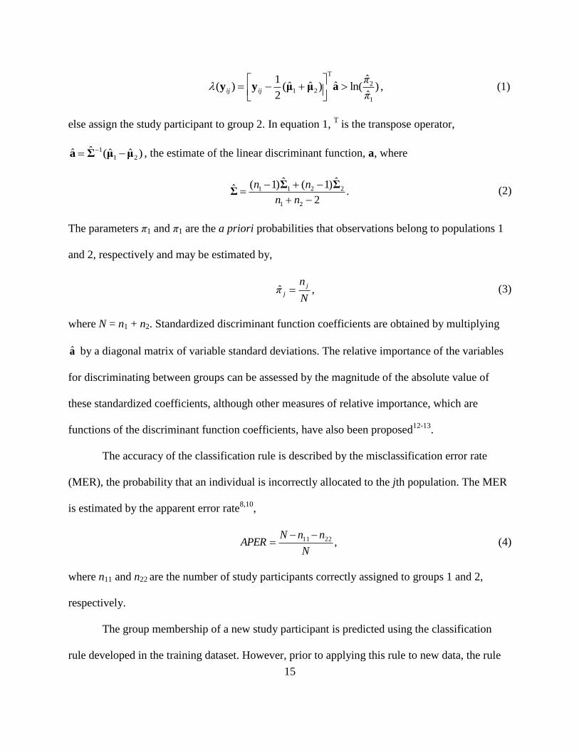
The linear DA classification rule is: Assign the ijth study participant to group 1 if

15

)ˆ

ˆln(ˆ)ˆˆ(

2

1)(

1

2

T

21π

πijij

aμμyy , (1)

else assign the study participant to group 2. In equation 1, T is the transpose operator,

)ˆˆ(ˆˆ21

1μμΣa , the estimate of the linear discriminant function, a, where

.2

ˆ)1(ˆ)1(ˆ

21

2211

nn

nn ΣΣΣ (2)

The parameters π1 and π1 are the a priori probabilities that observations belong to populations 1

and 2, respectively and may be estimated by,

,ˆN

nπ

j

j (3)

where N = n1 + n2. Standardized discriminant function coefficients are obtained by multiplying

a by a diagonal matrix of variable standard deviations. The relative importance of the variables

for discriminating between groups can be assessed by the magnitude of the absolute value of

these standardized coefficients, although other measures of relative importance, which are

functions of the discriminant function coefficients, have also been proposed12-13

.

The accuracy of the classification rule is described by the misclassification error rate

(MER), the probability that an individual is incorrectly allocated to the jth population. The MER

is estimated by the apparent error rate8,10

,

,2211

N

nnNAPER

(4)

where n11 and n22 are the number of study participants correctly assigned to groups 1 and 2,

respectively.

The group membership of a new study participant is predicted using the classification

rule developed in the training dataset. However, prior to applying this rule to new data, the rule

16

should be validated in order to assess its generalizability. Internal and external validation

techniques are discussed in a number of sources, including Timm10

and McLachlan11

.

Papers that provide a more detailed introduction to the theory and application of classical

linear DA include Huberty14

and Sherry7. A critical evaluation of the differences between DA

and logistic regression, another method that is commonly applied to classification problems, is

provided by Lei and Koehly15

. In general, DA is preferred when its underlying derivational

assumptions are satisfied because DA will have greater statistical power than logistic regression.

2.3 Examples of Potential Applications of Repeated Measures Discriminant

Analysis

Repeated measures DA procedures are applied to data collected on multiple occasions for

the same individual; often these data will arise in studies about development, maturation, or

aging processes. Below, we discuss a number of examples of the kinds of studies in which

repeated measures DA can be used.

Levesque, Ducharme, Zarit, Lachance, and Giroux16

were interested in classifying

husbands, who were care providers for functionally or cognitively impaired wives, into three

psychological distress groups based on changes in exposure to stress over time. The variables in

the study included objective stressors, such as wives’ functional impairment and memory and

behavioral problems, as well as subjective stressors such as role overload and relationship

deprivation. All variables were collected at two measurement occasions. Measures of change

over time, as well as some of the baseline measurements, were used to develop the classification

model using conventional linear DA. A total of N = 205 study participants provided data at the

17

baseline measurement occasion. More than one quarter (28.2%) of participants dropped out of

the study between the first and second measurement occasions; these individuals were excluded

from the analysis.

A second example comes from the study of Rietveld et al.17

. The researchers were

interested in discriminating monozygotic from dizygotic twins using measures of twin similarity

and confusion collected at ages six, eight, and 10 years. Self-report data on these measures were

obtained from both mothers and fathers. Classical linear DA was used to construct a separate

classification rule for each measurement occasion and for each parent, resulting in a total of six

rules. The rules were used to describe differences in classification accuracy over time and

between parents. Loss to follow up was substantial. While 691 twin pairs were initially recruited

into the study, by the third measurement occasion (i.e., age 10), mothers’ evaluations were only

available for 324 (46.9%) twin pairs and fathers’ evaluations were only available for 279

(40.4%) pairs. The classification rules were validated using a leave-one-out internal validation

method.

de Coster, Leentjens, Lodder, and Verhey18

applied classical linear DA to develop a

classification rule for first-time stroke patients using data collected on the 17 items of the

Hamilton Rating Scale for Depression (HAM-D) at one, three, six, and nine months post stroke.

A total of 206 patients were classified as depressed or not depressed; the depression diagnosis

was assigned based on the Structured Clinical Interview for the DSM-IV. The measurements

collected prior to the diagnosis of depression were used to classify patients into groups using

classical linear DA. The following HAM-D items were most important for discriminating

between depressed and non-depressed patients: depressed mood, reduced appetite, thoughts of

suicide, psychomotor retardation, psychic anxiety, and fatigue. Loss to follow up was small (i.e.,

18

about 10%).

2.4 Repeated Measures Discriminant Analysis

While the previous section illustrates the kinds of studies in which repeated measures DA

procedures can be applied, the authors of these studies used the classical linear DA procedure

instead. The application of classical linear DA to repeated measures data has been criticized for a

number of reasons19-20

: (a) observations with missing values are removed from analysis via

casewise deletion, (b) covariates are difficult to include, and (c) the classical DA procedure

cannot be applied to high dimensional data in which N is less than the product of the number of

repeated measurements and the number of variables.

Research about repeated measures DA has primarily been undertaken for PDA

procedures, rather than DDA procedures. Early research about PDA focused on procedures based

on the growth curve model21-23

as well as a stagewise discriminant, regression, discriminant

(DRD) procedure24

. Under the latter procedure, DA is applied separately to the data from each

measurement occasion. The discriminant function coefficients estimated at each measurement

occasion are then entered into a linear regression model and DA is applied to the slope and

intercept coefficients from this regression model. In terms of DDA procedures, Albert and

Kshirsagar25

developed two procedures for univariate repeated measures data, which are used to

evaluate the relative importance of the measurement occasions for discriminating amongst

groups. The first procedure is based on repeated measures multivariate analysis of variance

(MANOVA) while the second procedure is based on the growth curve model of Pothoff and

Roy26

.

19

To introduce DA procedures for repeated measures data, denote yl (l = 1 ,…, N) as the

vector of observations for the lth study participant, where the first nj observation vectors are for

participants in group 1 and the remaining observation vectors are for individuals in group 2. In

the case of univariate repeated measures data, that is, data that are collected on multiple

measurement occasions for a single variable, yl has dimension pl × 1, where pl is the number of

measurement occasions for the lth individual. In multivariate repeated measures data, that is, data

that are collected on multiple measurement occasions for two or more variables, yl has dimension

qpl × 1, where q is the number of variables. For simplicity, all procedures will be described for

the case pl = p.

2.4.1 The Covariance Pattern Model

The covariance pattern model was originally proposed by Jenrich and Schlutcher27

. For

univariate repeated measures data, the model is given by

yl = Xlβ + εl, (5)

where β is the k × 1 vector of parameters to be estimated, Xl is the p × k design matrix that

defines groups membership, and εl ~ Np(0, Σ). Group means are computed from estimates of the

fixed effects parameters, that is, βXyμ ˆ)(Eˆlll . This model assumes Σ has a functional form

such as compound symmetric (CS) or first-order autoregressive (AR-1). The CS covariance

structure assumes equal correlation between pairs of measurement occasions and constant

variance across the occasions. The assumption of equi-correlation, regardless of the time lag

between measurement occasions, may not be realistic in data collected over time, where the

magnitude of correlation often decreases as the time lag between measurement occasions

20

increases. The AR-1 covariance structure assumes the correlation between pairs of measurement

occasions decays over time but the variance remains constant across the occasions 28

. By

assuming a functional form for Σ, the number of variance and covariance parameters to estimate

is reduced, which may result in improved classification accuracy and is advantageous to ensure

the data are not overfit when total sample size is small relative to the number of measurement

occasions. For example, in a study with p = 4 repeated measurements, there are p(p + 1)/2 =

4(5)/2 = 10 parameters to estimate when Σ is unstructured as compared to two parameters to

estimate (one correlation and one variance) when a CS or AR-1 structure is assumed.

Repeated measures DA procedures based on the covariance pattern model can

accommodate time-invariant covariates, that is, explanatory variables that do not change across

the measurement occasions28

. The inclusion of covariates in the model may help to improve

classification accuracy. As well, it is possible to specify a mean structure for the model, such as

assuming that the means remain constant over time 29

, which reduces the number of mean

parameters to estimate and therefore may further improve classification accuracy.

Repeated measures DA based on the covariance pattern model for univariate repeated

measures data is described by Roy and Khattree29

. Under a CS structure, the authors showed, via

statistical proof that the classification rule does not depend on Σ. That is, assign the lth subject to

group 1 if

p,yp

k

lkl

2

ˆˆ)( 21

1

y (6)

else, allocate to group 2. In equation 6, ylk is the observation for the lth study participant on the

kth repeated measurement,

p

k

jkj p1

1 ˆˆ and jk is the estimated mean for the jth group on the

21

kth repeated measurement. By comparison, for an AR-1 structure the classification rule depends

on the correlation parameter, , as well as the estimated group means.

Repeated measures DA based on the covariance pattern model have also been described

for multivariate repeated measures data30-32

. Briefly, the covariance matrix of the repeated

measurements is assumed to have a Kronecker product structure, denoted by the notation

qp ΣΣΣ , where Σp is the covariance matrix of the repeated measurements and Σq is the

covariance matrix of the variables. A Kronecker product structure assumes that the covariance

matrix of the repeated measurements is constant across all variables; adopting this structure

results in a substantial reduction in the number of parameters to estimate. For example, with p =

4 and q = 3, there are a total of 4(5)/2 + 3(4)/2 = 16 covariance parameters to estimate under a

Kronecker product structure as compared to 12(13)/2 = 78 parameters to estimate when an

unstructured covariance is assumed. Roy and Khatree30

also describe models in which the

multivariate mean vector is assumed to have a specific function form (i.e., constant mean) over

time, although they do not investigate the effects of classification accuracy when the mean

structure is misspecified. Misspecification of the covariance structure in both univariate and

multivariate repeated measures analyses may result in increased misclassification rates. The

effects of misspecification are considered in a subsequent section of this manuscript. Graphic

exploration of the data, likelihood ratio tests, and penalized log-likelihood measures such as the

Akaike information criterion (AIC) have been recommended to guide the selection of a well-

fitted model with an appropriate covariance structure 28

.

22

2.4.2 The Linear Mixed-Effects Model

For univariate repeated measures data, the linear mixed-effects model is

lllll εdZβXy , (7)

where β is the k × 1 vector of fixed effect parameters, Xl is the p × k matrix of corresponding

covariates, and Zl is the p × s design matrix associated with the s × 1 vector of subject-specific

random effects dl. The error vector εl ~ Np(0, Ul) and the random effects vector dl ~ Ns(0, Gl) are

assumed to be independent. The subject-specific covariance matrix is defined as

lllll UZGZΣ T . (8)

A repeated measures DA procedure based on the mixed-effects model was first proposed by

Choi33

. Subsequently, Tomasko et al.20

developed procedures that assume various covariance

structures (such as CS and AR-1) for U, the covariance matrix of the residual errors; the

application of these procedures was illustrated by Wernecke, Kalb, Schink, and Wegner34

. The

classification rule is: Assign the lth study participant to group 1 if

)ˆ

ˆln()ˆˆ(ˆ)ˆˆ(

2

1)(

1

221

1

T

21π

πlllllll

μμΣμμyy , (9)

else, assign the participant to group 2. In equation 9, jlμ is the lth subject-specific mean for the

jth group. Maximum likelihood methods are used to estimate jlμ and Σ . A strength of DA

based on the linear mixed-effects model is that both time-varying and time-invariant covariates

can be accommodated in the model; covariate information may help to reduce misclassification

error. Moreover, this model can accommodate an unequal number of measurements per

individual.

Gupta35

extended Choi’s33

methodology to develop DA procedures based on the linear

23

mixed-effects model for multivariate repeated measures data. Roy19

proposed a classification

procedure for incomplete multivariate repeated measures data based on the multivariate linear

mixed-effects model that assumes a Kronecker product structure for the covariance matrix of the

residual errors. Marshall, De la Cruz-Mesia, Quitanna, and Baron36

developed classification

procedures based on the bivariate non-linear mixed-effects model that assumes a Kronecker

product structure for the residual error covariance matrix.

2.4.3 Comparisons Amongst Procedures

Research about the performance of different repeated measures DA procedures has been

limited. Roy and Khattree30-31

used simulation techniques to compare procedures based on

different covariance structures for univariate and multivariate repeated measures data. They

found that for univariate repeated measures data, the average APER for a procedure based on an

unstructured covariance was larger than the APER for procedures based on CS and AR-1

structures, regardless of the form of the population covariance. However, for multivariate

repeated measures data, a misspecified Kronecker product covariance structure resulted in a

higher APER than a correctly specified Kronecker product covariance structure. One study that

investigated DA procedures based on the mixed-effects model20

found that when sample size

was small, procedures that specified a covariance structure for the residual errors generally had

lower APERs than a procedure that adopted an unstructured covariance. However, for moderate

to large sample sizes, the increase in classification accuracy was often negligible. None of the

comparative studies that have been conducted to date have investigated the effect of a

misspecified mean structure on the APER.

24

The effect of missing data on classification accuracy was studied by Roy19

. She compared

the accuracy of a classification procedure based on the multivariate mixed-effects model to the

accuracy of a non-parametric classification procedure that used a multiple imputation method to

fill in the missing observations. The assumption underlying both models is that the data are

missing at random (MAR)37

. She found that the APER for the mixed-effects procedure was less

than the median error rate for the procedure based on the multiple imputation method. Roy

suggested that because the multiple imputation method introduces noise into the data, it may not

always be the optimal method to use.

2.5 Implementing Repeated Measures Discriminant Analysis

Covariance pattern models and mixed-effects models can be fit to univariate and

multivariate repeated measures data using the MIXED procedure in SAS38

. These models have

been described in several sources39-41

. Covariance pattern models are specified using a

REPEATED statement to identify the repeated measurements and define a functional form for

the covariance matrix. Mixed-effects models are specified using a RANDOM statement to

identify one or more subject-specific effects; a REPEATED statement may also be included to

define a functional form for the covariance matrix of the residuals. In multivariate repeated

measures data, the MIXED procedure can also be used to specify a Kronecker product structure

for the covariance matrix. However, the MIXED statement is limited to specifying Σp as

unstructured, AR-1, or CS, and Σq as unstructured. The parameter estimates and covariances are

extracted from the MIXED output using ODS output and the classification rule is defined to

calculate the APER. This last step can be completed using programming software such as

25

SAS/IML.

To illustrate, we use a numeric example based on the dataset described by Nunez-Anton

and Woodworth42

, which consists of the percent correct scores on a sentence test administered to

two groups of study participants wearing different hearing implants1. The purpose of the analysis

is to develop a classification rule to distinguish between the two type of implants. All study

participants were deaf prior to connection of the implants. Data are available for 19 participants

in group 1 and 16 participants in group 2, and measurements were obtained at one, nine, 18, and

30 months after connection of the implants. A total of 14 study participants had complete data at

all four measurement occasions. The pattern of missing data is intermittent. For this analysis we

assume that the data follow a multivariate normal distribution and also that the missing

observations are MAR37

.

Table 2-1 provides information about the number of complete observations, means, and

standard deviations for each measurement occasions for the two groups. The raw data are

provided in Appendix 1, along with the SAS code to define the dataset, audio.

26

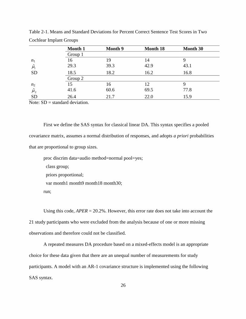
Table 2-1. Means and Standard Deviations for Percent Correct Sentence Test Scores in Two

Cochlear Implant Groups

Month 1 Month 9 Month 18 Month 30

Group 1

n1 16 19 14 9

29.3 39.3 42.9 43.1

SD 18.5 18.2 16.2 16.8

Group 2

n2 15 16 12 9

2 41.6 60.6 69.5 77.8

SD 26.4 21.7 22.0 15.9

Note: SD = standard deviation.

First we define the SAS syntax for classical linear DA. This syntax specifies a pooled

covariance matrix, assumes a normal distribution of responses, and adopts a priori probabilities

that are proportional to group sizes.

proc discrim data=audio method=normal pool=yes;

class group;

priors proportional;

var month1 month9 month18 month30;

run;

Using this code, APER = 20.2%. However, this error rate does not take into account the

21 study participants who were excluded from the analysis because of one or more missing

observations and therefore could not be classified.

A repeated measures DA procedure based on a mixed-effects model is an appropriate

choice for these data given that there are an unequal number of measurements for study

participants. A model with an AR-1 covariance structure is implemented using the following

SAS syntax.

27

data audio_long1;

set audio;

time=1; y=month1; output;




drop month1 month9 month18 month30;

run;

data audio_long; set audio_long1;

int=1;

timeg=time*group;

run;

proc sort data=audio_long;

by id;

run;

proc mixed data=audio_long method=ml;

class id group;

model y=time group time*group/ solution;

random intercept / subject=id v=1 solution;

repeated / type=ar(1) subject=id;

28

ods output v=vmat solutionf=parms_mat;

run;

The dataset audio_long1 converts the data into a person-period format and in audio_long,

we create new variables called timeg (interaction) and int (model intercept). The MIXED syntax

specifies the use of maximum likelihood estimation and implements a model containing the fixed

effects of time, group, and their interaction. The RANDOM statement specifies a random

intercept and requests the estimated covariance matrix for subject 1. The REPEATED statement

specifies an AR-1 structure for the residual errors. The ODS statement indicates that 1Σ will be

output to a new dataset named vmat, while the fixed-effects parameters are output to the dataset

parms_mat. Two additional models were fit to these data (syntax not shown), to identify a well-

fitting model for these data. One model included a random intercept and random slope, and the

second included the quadratic term for time as an additional model covariate. The former did not

result in improved model fit, as judged by the AIC, and the latter resulted in problems with

estimation of the covariance parameters. Appendix 2 provides example code used to extract the

ODS output into SAS/IML to implement the linear classification rule.

Fit statistics and APERs are provided in Table 2-2 for three models, to illustrate the effect

of modifying the covariance structure on classification accuracy.

29

Table 2-2: Fit Statistics and Apparent Error Rates (APER) for the Mixed-Effects Model with

Three Covariance Structures

Structure of lΣ AIC n11 n22 APER (%)

AR-1 877.2 12 12 31.4

CS 886.2 12 13 28.6

UN 876.3 14 16 14.3

Note: AR-1 = first-order autoregressive; CS = compound symmetric; UN = unstructured; AIC =

Aikake Information Criterion; n11 and n22 are the number of study participants correctly

classified to groups 1 and 2, respectively; APER = apparent error rate.

Overall, the model with an unstructured covariance had the lowest value of the AIC and

also resulted in the lowest APER. While no guidelines exist about acceptable magnitude of the

APER, it is possible to test for differences in APER values across models11, 43

.

Example syntax is provided in Appendix 2 that could be used to fit both a CS and AR-1

covariance pattern to these data. Given that the covariance pattern model is only applicable to

datasets with complete observations, this syntax is provided for illustration purposes.

2.6 Discussion

While research about repeated measures DA spans more than a 30-year period, there have

been a number of recent developments in PDA procedures based on covariance pattern and

mixed-effects models for univariate and multivariate repeated measures data. These

developments provide applied researchers with a number of options to develop accurate and

efficient classification rules when data are collected repeatedly on the same subjects. Several of

these procedures can be implemented using standard statistical software, although some

supplementary programming is required to implement the classification rule.

30

There are opportunities for further research about repeated measures DA procedures. For

example, there has been limited research about procedures for non-normal data and

heterogeneous group covariances. While the misclassification error rate of classical linear DA is

reasonably robust (i.e., insensitive) to outliers44

, heavy-tailed distributions may result in some

loss of classification accuracy and inflate the standard errors of discriminant function

coefficients. Non-parametric DA procedures, which do not assume a normal distribution of

responses, such as nearest neighbor classification procedures, have been investigated for

repeated measures data45

. PDA procedures based on the multivariate Box and Cox

transformation46

and a rank transformation method47

, which Baron48

found to perform well for a

number of different non-normal distributions, as well as distribution-free methods49

, have not yet

been investigated for repeated measures data. Roy and Khattree29-30

developed PDA procedures

for heterogeneous group covariances based on the covariance pattern model while Marshall and

Baron50

proposed PDA procedures based on the mixed-effects model for conditions of

covariance heterogeneity, which can be implemented using SAS software. Roy and Khattree30

showed in a single numeric example that when covariances are heterogeneous, a PDA procedure

for unequal group covariances had a lower APER than a procedure that assumed homogeneity of

group covariances. Additional research is needed to compare the classification accuracy of these

procedures across a range of conditions of heterogeneity, particularly when group sizes are

unequal, and to develop software to implement these procedures. As well, comparisons with

conventional linear DA could also be undertaken.

Non-ignorable missing data, that is, data that are missing not at random (Little & Rubin,

1987) is likely to affect the accuracy of DA classification rules. Pattern mixture and selection

models 51-53

have been proposed to adjust for potential bias in mixed-effects models when it

31

cannot be assumed that the mechanism of missingness is ignorable. Further research could

investigate the development of DA procedures based on these models.

Finally, other models could be investigated for repeated measures data. Examples include

extensions of the growth curve model25

to include random effects and machine learning models

for high dimensional data54

.

32

Acknowledgements

This research was supported by funding from the Manitoba Health Research Council, a Canadian

Institutes of Health Research (CIHR) New Investigator Award to the first author, and a CIHR

Vanier Graduate Scholarship to the second author.

33

References

1. Fisher, R. A. (1936). The use of multiple measurements in taxonomic problems. Annals

of Eugenics, 7, 179 – 188.

2. Huberty, C. J., & Olejnik S. (2006). Applied MANOVA and Discriminant Analysis. New

Jersey: Wiley.

3. Onur, E., Alkin, T., & Tural, U. (2007). Panic disorder subtypes: further clinical

differences. Depression and Anxiety, 24, 479 – 486.

4. Williams, D. L., Goldstein, G., & Minshew, N. J. (2006). The profiles of memory

function in children with autism. Neuropsychology, 20, 21 – 29.

5. Pyryt, M. C. (2004). Pegnato revisited: using discriminant analysis to identify gifted

children. Psychology Science, 46, 342 – 347.

6. Corcos, M., Loas, G., Sperana, M., Perez-Diaz, F., Stephan, P., Vernier, A., Lang, F.,

Nezelof, S., Bizouard, P., Veniss, J, L., & Jeammet, P. (2008). Risk factors for addictive

disorders: a discriminant analysis on 374 addicted and 513 nonpsychiatric participants.

Psychological Reports, 102, 435 – 449.

7. Sherry, A. (2006). Discriminant analysis in counseling psychology research. The

Counseling Psychologist, 34, 661 – 683.

8. Rencher, A. C. (2002). Methods of Multivariate Analysis. New Jersey: Wiley.

9. Tabachnick, B. G., & Fidell, L. S. (2007). Using Multivariate Statistics, 5th

Edition.

Boston: Allyn & Bacon.

10. Timm, N. H. (2006). Applied Multivariate Analysis. New York: Springer-Verlag.


34

York: Wiley.

12. Huberty, C. J., & Wisenbaker, J. M. (1992). Variable importance in multivariate group

comparisons. Journal of Educational Statistics, 17, 75 – 91.

13. Thomas, R. D. (1992). Interpreting discriminant functions: a data analytic approach.

Multivariate Behavioural Research, 27, 335 – 362.

14. Huberty, C. J. (1984). Issues in the use and interpretation of discriminant analysis.

Psychological Bulletin, 95, 156 – 171.

15. Lei, P., & Koehly, L. M. (2003). Linear discriminant analysis versus logistic regression:

A comparison of classification errors in the two-group case. The Journal of Experimental

Education, 72, 25 – 49. .

16. Levesque, L., Ducharme, F., Zarit, S. H., Lachance, L., & Giroux F. (2008). Predicting

longitudinal patterns of psychological distress in older husband caregivers: further

analysis of existing data. Aging and Mental Health, 12, 333 – 342.

17. Rietveld, M. J. H., van der Valk, J. C., Bongers, I. L., Stroet, T. M., Slagboom, P. E., &

Boomsma, D. I. (2000). Zygosity diagnosis in young twins by parental report. Twin

Research, 3, 134 – 141.

18. de Coster, L., Leentjens A. F. G., Lodder, J., & Verhey, F. R. J. (2005). The sensitivity

of somatic symptoms in post-stroke depression: a discriminant analytic approach.

International Journal of Geriatric Psychiatry, 20, 358 – 362.

19. Roy, A. (2006). A new classification rule for incomplete doubly multivariate data using

mixed effects model with performance comparisons on the imputed data. Statistics in

Medicine, 25, 1715 – 1728.

20. Tomasko, L., Helms, R. W., & Snappin, S. M. (1999). A discriminant analysis extension

35

to mixed models. Statistics in Medicine, 18, 1249 – 1260.

21. Azen S. P., & Afifi, A. A. (1972). Two models of assessing prognosis on the basis of

successive observations. Mathematical Biosciences, 14, 169 – 176.

22. Lee, J. C. (1982). Classification of growth curves. In Classification, Pattern Recognition,

and Reduction of Dimensionality. Handbook of Statistics, vol. 2, P. R. Krishnaiah and L.

N. Kanal, eds. (Amsterdam: North – Holland), pp. 121-137.

23. Albert, A. (1983). Discriminant analysis based on multivariate response curves: a

descriptive approach to dynamic allocation. Statistics in Medicine, 2, 95 – 106.

24. Afifi, A. A., Sacks, S. T., Liu, V. Y., Weil, M. H., & Shubin, H. (1971). Accumulative

prognostic index for patients with barbiturate, glutethimide and meprobamate

intoxication. New England Journal of Medicine, 285, 1497 – 1502.



26. Potthoff, R. F., & Roy, S. N. (1964). A generalized multivariate analysis of variance

model useful especially for growth curve problems. Biometrika, 51, 313 – 326.

27. Jenrich, R. I., & Schluchter, M. D. (1986). Unbalanced repeated measures models with

structural covariance matrices. Biometrics, 42, 805 – 820.

28. Fitzmaurice, G. M., Laird, N. M., & Ware, J. H. (2004). Applied Longitudinal Analysis.

New Jersey: Wiley.

29. Roy, A., & Khattree, R. (2005a). Discrimination and classification with repeated

measures data under different covariance structures. Communications in Statistics –

Simulation and Computation, 34, 167 – 178.


36


31. Roy, A., & Khattree, R. (2007). Classification of multivariate repeated measures data

with temporal autocorrelation. Advances in Data Analysis and Classification, 1, 175 –

199.

32. Krzysko, M., & Skorzybut, M. (2009). Discriminant analysis of a multivariate repeated

measures data with a Kronecker product structured covariance matrices. Statistical

Papers, 50, 817 – 855.

33. Choi, S. C. (1972). Classification of multiply observed data. Biometrische Zeitschrift, 14,

8 – 11. .

34. Wernecke, K. D., Kalb, G., Schink, B., & Wegner, B. (2004). A mixed model approach

to discriminant analysis with longitudinal data. Biometrical Journal, 46, 246 – 254.

35. Gupta, A. K. (1986). On a classification rule for multiple measurements. Computer

Mathematics and Applications, 12, 301 – 308.


analysis for longitudinal data with multiple continuous responses and possibly missing

data. Biometrics, 65, 69 – 80.

37. Little, R. J. A., & Rubin, D.B. (1987). Statistical Analysis with Missing Data. New York:

Wiley.

38. SAS Institute Inc. (2008). SAS/STAT User's Guide, Version 9.2. Cary, NC: SAS Institute

Inc.

39. Littell, R. C., Pendergast, J., & Natarajan, R. (2000). Tutorial in biostatistics: modelling

covariance structure in the analysis of repeated measures data. Statistics in Medicine, 19,

1793 – 1819.

37

40. Singer, J. D. (1998). Using SAS PROC MIXED to fit multilevel models, hierarchical

models, and individual growth models. Journal of Educational and Behavioral Statistics,

24, 323 – 355.

41. Thiebaut, R., Jacqmin-Gadda, H., Chene, G., Leport, C., & Commenges. D. (2002).

Bivariate linear mixed models using SAS PROC MIXED. Computer Methods and

Programs in Biomedicine, 69, 249 – 256.

42. Nunez-Anton, V., & Woodworth, G. G. (1994). Analysis of longitudinal data with

unequally spaced observations and time-dependent correlated errors. Biometrics, 50, 445

– 456.

43. Lachenbruch, P. A., & Mickey, M. R. (1968). Estimation of error rates in discriminant

analysis. Technometrics, 10, 1 – 11.

44. Lee, C. K., & Ord, J. K. (1990). Discriminant analysis via least absolute deviations.

Decision Sciences, 21, 86 – 96.

45. Bagui, S. C., & Mehra, K. L. (1999). Classification of multiple observations using multi-

stage nearest rank neighbor rule. Journal of Statistical Planning and Inference, 76, 163 –

183.

46. Velilla, S., & Barrio, J. A. (1994). A discriminant rule under transformation.

Technometrics, 36, 348 – 353.

47. Conover, W. J., & Iman, R. L. (1980). The rank transformation as a method of

discrimination with some examples. Communications in Statistics, 9, 465 – 487.

48. Baron, A. E. (1991). Misclassification among methods used for multiple group

discrimination: the effects of distributional properties. Statistics in Medicine, 10, 757 –

766.

38

49. Burr, T., & Doak, J. (2007). Distribution-free discriminant analysis. Intelligent Data

Analysis, 11, 651 – 662.

50. Marshall, G., & Baron, A. E. (2000). Linear discriminant models for unbalanced

longitudinal data. Statistics in Medicine, 19, 1969 – 1981.

51. Hedeker, D., & Gibbons, R. D. (1997). Application of random-effects pattern-mixture

models for missing data in longitudinal studies. Psychological Bulletin, 2, 64 – 78. .

52. Little, R. J. A. (1993). Pattern-mixture models for multivariate incomplete data. Journal

of the American Statistical Association, 88, 125 – 134.

53. Little, R. J. A. (1995). Modeling the dropout mechanism in repeated-measures studies.

Journal of the American Statistical Association, 90, 1112 – 1121.

54. Hastie, T., Tibshirani, R., & Friedman, J. H. (2001). Elements of Statistical Learning:

Data Mining, Inference, and Prediction. New York: Springer.

39

Appendix 2-1. Example Dataset for Repeated Measures Discriminant Analysis

Id group month1 month9 month18 month30

1 1 28 33 47 59

2 1 . 13 21 26

3 1 50 46 . .

4 1 13 30 42 .

5 1 43 61 67 .

6 1 . 59 57 61

7 1 21 38 . .

8 1 . 10 20 31

9 1 14 35 37 44

10 1 16 33 45 52

11 1 31 50 43 62

12 1 4 11 14 15

13 1 0 18 35 38

14 1 50 55 59 .

15 1 38 59 61 .

16 1 67 68 . .

17 1 46 58 52 .

18 1 25 42 . .

19 1 22 27 . .

20 2 33 66 . .

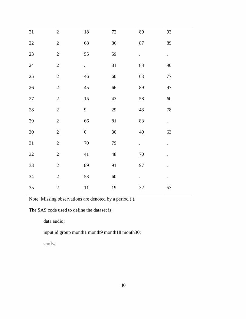
40

21 2 18 72 89 93

22 2 68 86 87 89

23 2 55 59 . .

24 2 . 81 83 90

25 2 46 60 63 77

26 2 45 66 89 97

27 2 15 43 58 60

28 2 9 29 43 78

29 2 66 81 83 .

30 2 0 30 40 63

31 2 70 79 . .

32 2 41 48 70 .

33 2 89 91 97 .

34 2 53 60 . .

35 2 11 19 32 53

Note: Missing observations are denoted by a period (.).

The SAS code used to define the dataset is:

data audio;

input id group month1 month9 month18 month30;

cards;

41

Appendix 2-2. Illustration of SAS syntax to Implement Discriminant Analysis Procedures

based on Mixed-Effects and Covariance Structure Models

Mixed-effects model

This SAS/IML syntax reads the SAS datasets from the ODS output (see section 5) for the

MIXED procedure and demonstrates the application of the classification rule to the data for the

first study participant.

proc iml;

reset noname;

use audio_long;

read all var {id int time group timeg y} into tempmat where (y >= 0);

use parms_mat;

read all var {‘estimate’} into beta;

beta1a=beta[1:3];

beta1b=beta[5];

beta1=beta1a//beta1b;

use vmat;

read all var {‘index’ ‘col1’ ‘col2’ ‘col3’ ‘col4’} into vmat;

ntot=35;

n1=19;

n2=16;

discrim=j(ntot,1,.);

count=j(ntot,1,.);

42

**this portion of the code applies the classification rule to the data for subject id=1**;

subj=1;

xmatss1=tempmat[1:4,2:5];

xmatss2=xmatss1;

xmatss2[,3]=0;

ymatss=tempmat[1:4,6];

vmatss=vmat[1:4,3:6];

mu1=xmatss1*beta1;

mu2=xmatss2*beta1;

discrim[subj]=(ymatss-0.5*(mu1+mu2))`*(inv(vmatss)*(mu1-mu2));

print ‘Discriminant function for subject id=1’;

print discrim[format=6.2];

if discrim[subj] >=ln(n2/n1) then count[subj]=1;

else count[subj]=0;

quit;

Covariance pattern model

This SAS/IML syntax applies the DA classification rule defined in equation 6, which is based on

a CS covariance structure. It also applies a classification rule based on an AR-1 covariance

structure. Unlike the previous analyses, neither of these models includes subject-specific effects.

**DA BASED ON COVARIANCE PATTERN MODEL WITH CS STRUCTURE**;

43

proc iml;

reset noname;

use audio;

read all var {month1 month9 month18 month30} into y;

p=4;

n1=19;

n2=16;

nsum = n1+n2;

dsum = j(nsum,1,.);

do i = 1 to nsum;

d1 = sum(y[i,]);

if i = 1 then dsum = d1;

else dsum = dsum//d1;

end;

y1 = y[1:n1,];

y2 = y[(n1+1):nsum, ];

ybar1 = y1[+,]/n1;

ybar2 = y2[+,]/n2;

ybar = ybar1//ybar2;

yp = j(1,p,1);

mu1 = yp*(ybar1`)/p;

mu2 = yp*(ybar2`)/p;

d = j(nsum,1,.);

44

countn = 0;

countn1 = 0;

do t = 1 to nsum;

if dsum[t] >= (mu1 + mu2)#p/2 then countn = countn + 1;

end;

do t = 1 to n1;

if dsum[t] >= (mu1 + mu2)#p/2 then countn1 = countn1 + 1;

end;

a = n1 - countn1;

aper = (countn - countn1 + a)*100/nsum;

print 'APER';

print aper[format=6.2];

quit;

**DA BASED ON COVARIANCE PATTERN MODEL WITH AR-1 STRUCTURE**;

proc mixed data = audio_long method = ml;

class id group;

model y = time group time*group /solution;

repeated / type = ar(1) subject = id;

ods output covparms = cov;

run;

proc iml;

45

reset noname;

use audio;

read all var {month1 month9 month18 month30} into z;

use cov;

read all var {'estimate'} into v;

rho = v[1];

n1=19;

n2=16;

nsum =n1+n2;

p = 4;

dtot = j(nsum, 1, .);

dtot2 = j(nsum,1, .);

do i = 1 to nsum;

dtot[i] = sum(z[i,]);

end;

do k = 1 to nsum;

dtot2[k] = sum(z[k,2:p-1]);

end;

mdtot = dtot/p;

mdtot2 = dtot2/(p-2);

z1 = z[1:n1, ];

z2 = z[(n1+1):nsum, ];

46

zbar1 = z1[+,]/n1;

zbar2 = z2[+,]/n2;

zbar = zbar1//zbar2;

zp = j(1,p,1);

mu1 = zp*(zbar1`)/p;

mu2 = zp*(zbar2`)/p;

/**Allocation Rule****/

zcount = 0;

zcount1=0;

do ir = 1 to nsum;

if (p*mdtot[ir] - rho*(p-2)*mdtot2[ir])>= (1/2)*(p - rho*(p-2))*(mu1+ mu2) then zcount

= zcount+1;

end;

do ir = 1 to n1;

if (p*mdtot[ir] - rho*(p-2)*mdtot2[ir])>= (1/2)*(p - rho*(p-2))*(mu1+mu2) then zcount1

= zcount1+1;

end;

z1= n1 - zcount1;

aper = (zcount - zcount1+ z1)*100/nsum;

print ’APER';

print aper[format = 6.2];

quit;

47

Chapter 3: Descriptive Discriminant Analysis for Repeated Measures Data

Abbreviations

AR-1 = First-order autoregression

CS = Compound symmetry



DFC = Discriminant function coefficient

MANOVA = Multivariate analysis of variance

RMDA = Repeated measures discriminant analysis

RMDDA = Repeated measures descriptive discriminant analysis

48

3.1 Introduction

The previous chapter reviews various repeated measures discriminant analysis (RMDA)

procedures for predicting group membership and describing group separation in univariate and

multivariate repeated measures data. This includes discriminant analysis (DA) procedures based

on growth curve, mixed-effects, and covariance structure models1-3

. Although these procedures

are based on different underlying assumptions, they result in better classification accuracy than

the conventional DA procedure when the underlying model assumptions are satisfied. DA

procedures based mixed-effects models are advantageous over the conventional DA procedure in

that it can be accommodate both time variant and time invariant covariates and can also be used

to predict group memberships when in studies with missing observations. Similarly, DA

procedures based on covariance structure models, which assume constant means and

parsimonious covariance structures are advantageous when the sample size is small. A

summarized description of strengths and limitations of the existing RMDA procedures is

provided in Table 3-1. Although these RMDA procedures have been specifically developed for

prediction of group membership in repeated measures data, there is less emphasis on the

description of group separations (i.e., descriptive discriminant analysis, DDA).

49

Table 3-1. Repeated Measures Models for Discriminant Analysis

Model Description Advantages Limitations

Covariance

Structure Models

1. The proposed DA

procedures assume

constant repeated

measures means and

parsimonious covariance

structures for univariate

and multivariate repeated

measures data.

2. Estimation of the DFCs

is based on the maximum

likelihood estimation

method.

1. Can be used in

studies with small

sample size.

2. Results in better

classification

accuracy than the

conventional DA

procedure.

1. Assumes complete

data on all

measurement

occasions

2. Classification

accuracy may be

reduced due to mis-

specification of

covariance structure.

3. The assumption of

constant means may

not be tenable in

repeated measures

studies with non-

constant means.

Mixed-effects

models

1. The proposed DA procedure

is based means and

covariances estimated from a

mixed-effects model that

assume parsimonious

1. DA procedure can

be used when data are

missing at random.

2. Can accommodate

covariates to improve

1. Can be

computationally

intensive in

multivariate repeated

measures data.

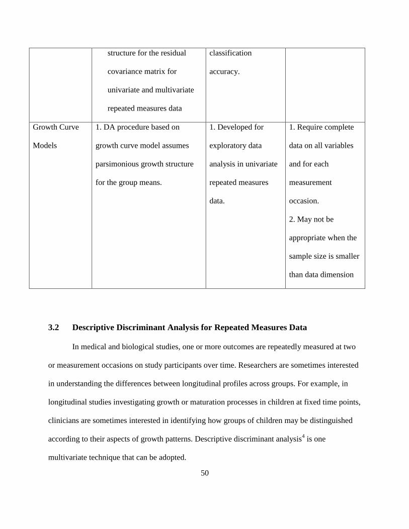
50

structure for the residual

covariance matrix for

univariate and multivariate

repeated measures data

classification

accuracy.

Growth Curve

Models

1. DA procedure based on

growth curve model assumes

parsimonious growth structure

for the group means.

1. Developed for

exploratory data

analysis in univariate

repeated measures

data.

1. Require complete

data on all variables

and for each

measurement

occasion.

2. May not be

appropriate when the

sample size is smaller

than data dimension

3.2 Descriptive Discriminant Analysis for Repeated Measures Data

In medical and biological studies, one or more outcomes are repeatedly measured at two

or measurement occasions on study participants over time. Researchers are sometimes interested

in understanding the differences between longitudinal profiles across groups. For example, in

longitudinal studies investigating growth or maturation processes in children at fixed time points,

clinicians are sometimes interested in identifying how groups of children may be distinguished

according to their aspects of growth patterns. Descriptive discriminant analysis4 is one

multivariate technique that can be adopted.

51

Let Yij be the p 1 random vector of observed measurements for the ith study participant

(i = 1, ...,nj; N = n1 + n2) in the jth group (j = 1, 2). It is assumed that Yij ~ Np(μj, Σj), where μj

and Σj are the population mean vector and covariance for the jth group. DDA can be expressed as

a regression model, where discriminant function score lij is expressed as

ijij cl ya (1)

where

)ˆˆ(ˆ)ˆ(2

121

1T

21 μμΣμμ c , (2)

and a corresponds to the vector of discriminant function coefficients given by

)ˆˆ(ˆˆ21

1μμΣa , (3)

,2

ˆ)1(ˆ)1(ˆ 2211

N

nn ΣΣΣ (4)

and

.ˆj

n

1i

ij

jn

j

y

μ (5)

The discriminant function coefficients (DFCs) can be used to rank order variables according to

their ability to discriminate between groups5-6

. Although the conventional DDA procedure may

be used to describe group separation in repeated measures data, it does not take advantage of the

special structure the data and may not be appropriate in studies with sample sizes.

Descriptive discriminant analysis procedures for repeated measures data that assume

parsimonious means and/or covariance structures are alternative approach to describing group

separation in repeated measures data. Earlier references to repeated measures descriptive

discriminant analysis (RMDDA) include the two RMDDA procedures developed by Albert and

52

Kshirsagar7 to evaluate the relative importance of the measurement occasions for discriminating

amongst groups. The first procedure is based on repeated measures multivariate analysis of

variance (MANOVA) while the second procedure is based on the growth curve model of Pothoff

and Roy8. While the former places no restriction on the means and covariance structures, the

latter assume parsimonious growth curve structures for the group means and developed goodness

of fit tests to determine the appropriate growth curve for the means. However, these two

procedures make no assumptions about the covariance structures for the data.

In this chapter and subsequent ones, we investigate the use of DFCs derived from RMDA

procedures that assume parsimonious covariance and mean structures for describing group

separation in repeated measures data. More specifically, RMDA procedures that assume

parsimonious means and/or covariance structures are investigated. This includes RMDA

procedures that assume constant means and compound symmetric (CS) or first order

autoregressive (AR-1) covariance structures for predicting group memberships in univariate

repeated measures data. Also, RMDA procedures that assume structured and unstructured group

means and Kronecker product covariance structures have also been developed for multivariate

repeated measures data. These procedures are particularly advantageous for describing group

separation in high-dimensional longitudinal studies where the sample size is small relative to the

dimension of the data.

However, previous research on the DFCs from the conventional DDA procedure for

multivariate group designs has shown that DFCs are sensitive to a variety of data characteristics,

which may consequently influence the ability to correctly rank order a set of correlated variables.

William and Titus9 used Monte Carlo methods to investigate the influence of several data

characteristics on bias and error in the DFCs of the conventional DA procedure. Their study

53

showed that the bias and error in the estimated DFCs are influenced by the number of outcomes,

the magnitude of separation between group means, and the magnitude of correlation among the

variables. However, conclusions from this study are limited because the conditions investigated

are limited to normally distributed data and for certain selected mean configurations and

correlation structures.

For RMDA procedures that assume parsimonious structures on the means and

covariances, previous research suggests that the assumption of parsimony improves the accuracy

of prediction of group membership3, a mis-specification of the covariance structure may

influence the classification accuracy of the procedures10

. To investigate the accuracy and

precision of DFCs derived from RMDA procedures for describing group separation, we

hypothesize that in addition to the influence of a variety of data characteristics, the DFCs of

these procedures may be influenced by the assumption of parsimony on the means and

covariance structures as well as covariance and mean structure mis-specification.

The next chapter is a manuscript that investigates the effects of the assumptions of

parsimony and mis-specification of RM mean and covariance structures on bias and error in the

discriminant function coefficients of repeated measures DA procedures based on constant mean

structures using Monte Carlo techniques. This manuscript has been accepted for publication in

the Journal of Modern Applied Statistical Methods

54

References



2. Lee, J. C. (1982). Classification of growth curves. In Classification, Pattern Recognition,

and Reduction of Dimensionality. Handbook of Statistics, vol. 2, P. R. Krishnaiah and L.

N. Kanal, eds. (Amsterdam: North – Holland), pp. 121 – 137.

3. Roy, A., & Khattree, R. (2005). Discrimination and classification with repeated measures




of Eugenics, 7, 179 – 188.



6. Thomas, R. D. (1992). Interpreting discriminant functions: a data analytic approach.

Multivariate Behavioural Research, 27, 335 – 362.



8. Potthoff, R. F., & Roy, S. N. (1964). A generalized multivariate analysis of variance

model useful especially for growth curve problems. Biometrika, 51, 313 – 326.

9. Williams, B. K., & Titus, K. (1988). Assessment of sampling stability in ecological

applications of discriminant analysis. Ecology, 69, 1275 – 1285.


with temporal autocorrelation. Advances in Data Analysis and Classification, 1; 175 –

55

199.

56

Chapter 4. Discriminant Analysis for Repeated Measures Data: Effects of Mean and

Covariance Mis-specification on Bias and Error in Discriminant Function

Coefficients

Tolulope T. Sajobi1

Lisa M. Lix1, 2

William H. Laverty2

Longhai Li2

1. School of Public Health, University of Saskatchewan, Saskatoon, Canada

2. Department of Mathematics & Statistics, University of Saskatchewan, Saskatoon, Canada

A shortened version of this chapter has been accepted for publication in Journal of Modern

Applied Statistical Methods as of May 2011. This chapter contains additional details in the

Appendix. This manuscript has been re-organized in this chapter to meet the dissertation

requirements of the University of Saskatchewan. My contribution to this published manuscript

includes the review of the literature, statistical analysis using an example dataset, and preparation

of the manuscript for publication.

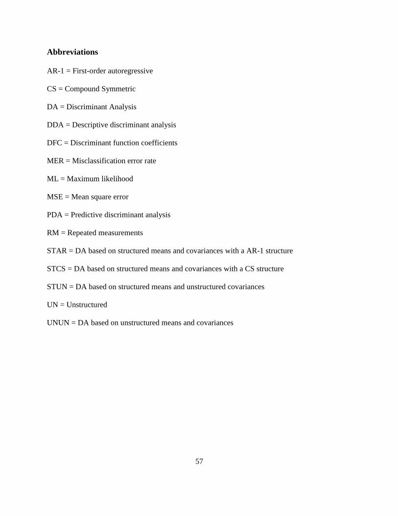
57

Abbreviations

AR-1 = First-order autoregressive

CS = Compound Symmetric

DA = Discriminant Analysis


DFC = Discriminant function coefficients

MER = Misclassification error rate

ML = Maximum likelihood

MSE = Mean square error


RM = Repeated measurements

STAR = DA based on structured means and covariances with a AR-1 structure

STCS = DA based on structured means and covariances with a CS structure

STUN = DA based on structured means and unstructured covariances

UN = Unstructured

UNUN = DA based on unstructured means and covariances

58

Abstract

Discriminant analysis (DA) procedures based on parsimonious mean and/or covariance

structures have recently been proposed for repeated measures (RM) data. This paper investigates

bias and means square error of discriminant function coefficients (DFCs) of these DA procedures

when mean and/or covariance structures are correctly specified and misspecified.

Key Words: bias; discriminant function coefficients; mean square error; multivariate; model

misspecification

59

4.1 Introduction

Linear discriminant analysis (DA) is a multivariate procedure, originally proposed by

Fisher1, for predicting group membership (predictive discriminant analysis; PDA) and/or

describing group separation (descriptive discriminant analysis; DDA) on multiple variables2. The

classical linear PDA procedure has also been applied to repeated measures (RM) data3-4

, in

which study participants are measured on a single variable at two or more occasions. Classical

linear DA will not result in an efficient classification rule in multivariate or RM data when there

are a large number of variables or measurement occasions relative to sample size. In recent

years, a number of PDA procedures for RM data have been proposed5-9

. Specifically, Roy and

Khattree6-7

developed DA procedures based on parsimonious mean and covariance structures for

both univariate (i.e., measurements on one outcome variable) and multivariate (i.e.,

measurements on two or more outcome variables) RM data to address the issue of classification

efficiency when sample size is small. For univariate RM data, the proposed procedures based on

a constant RM mean vector and either a compound symmetric (CS) or first-order autoregressive

(AR-1) covariance. While these procedures can result in efficient classification rules in high-

dimensional data8, they can also result in inflated misclassification error rates (MERs) when the

mean and/or covariance structure is/are incorrectly specified.

Although these procedures were originally developed for PDA, the discriminant function

coefficients (DFCs) that are produced can be used for DDA, that is, to quantify the relative

importance of the measurement occasions for discriminating amongst groups10

. In classical linear

DA, it is known that bias and error variation of DFCs is influenced by a variety of characteristics

of the data, including degree and pattern of separation between groups (i.e., group mean vectors),

60

and magnitude of correlation among the outcome variables11-12

. However, to date, there has been

little, if any research, about the effects of mis-specifying the mean and/or covariance structure on

DDA procedures for RM data.

The purpose of this study is to investigate the effects of RM mean and/or covariance

misspecification on bias and error in DFCs of DDA procedures based on constant mean vectors

and/or structured covariance matrices in univariate RM data. The manuscript is organized as

follows: First, the investigated DA procedures are described. The results of a Monte Carlo study,

which was conducted to investigate the effects of mean and covariance structure mis-

specification under a variety of data-analytic conditions, are presented. The manuscript

concludes with some considerations about selecting a DDA procedure for RM data.

4.2 Estimation of DFCs in DA Procedures for RM Data

Throughout this manuscript, we focus on the case of g = 2 groups, although all procedures

can also be generalized to g > 2. In general, the number of uncorrelated DFC vectors is equal to g

– 1.

Let yij be the p 1 random vector of observed measurements for the ith study participant (i

= 1, ...,nj; N = n1 + n2) in the jth group (j = 1, 2). It is assumed that yij ~ Np(μj, Σj), where μj and

Σj are the population mean vector and covariance for the jth group and are estimated by jμ and

jΣ , respectively. The linear DFC vector is estimated by

)ˆˆ(ˆˆ21

1μμΣa . (1)

For the conventional linear DA procedure,

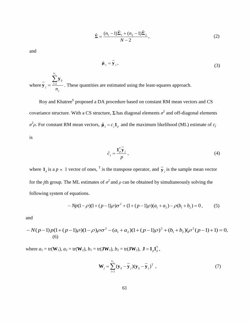
61

,2

ˆ)1(ˆ)1(ˆ 2211

N

nn ΣΣΣ (2)

and

,jj yμ ˆ

(3)

wherej

n

i

ij

jn

j

1

y

y . These quantities are estimated using the least-squares approach.

Roy and Khatree6 proposed a DA procedure based on constant RM mean vectors and CS

covariance structure. With a CS structure, Σ has diagonal elements σ2 and off-diagonal elements

σ2ρ. For constant RM mean vectors, pjj c 1μ ˆ and the maximum likelihood (ML) estimate of cj

is

pc

jp

j

y1T

ˆ , (4)

where p1 is a p 1 vector of ones, T is the transpose operator, and

jy is the sample mean vector

for the jth group. The ML estimates of σ2

and ρ can be obtained by simultaneously solving the

following system of equations.

0)())()1(1())1(1)(1( 2121

2 bbaappNp , (5)

and

,0)1)1()(())1(1)(()1)()1(1()1( 2

21

2

21

2 pbbpaapppN

(6)

where a1 = tr(W1), a2 = tr(W2), b1 = tr(JW1), b2 = tr(JW2), T

pp11J ,

T

1

)()(jij

n

i

jijj

j

yyyyW

, (7)

62

and tr is the trace operator. The DFCs are estimated by substituting the ML estimates of Σ and jμ

in equation 1.

Roy and Khattree6 proposed a DA procedure based on constant RM mean vectors and AR-1

covariance structure. With an AR-1 structure, Σ has diagonal elements σ2 and off-diagonal

elements σ2ρ

l, where l is the number of lags between measurement occasions. Estimates of cj, σ

2,

and ρ are obtained by simultaneously solving

0)2()2( 21 jjjj mppmpccp , (8)

,0))1(2)2)((()2(

)2()2()1(

22

22

2

1133

2

322

22

2

21111

2

1

22

pppcncncn

cnNp

(9)

and

.0)}1()1()22(){(

})({})({

})({)1()1(

22

22

2

11

3

2

333222

2

22211

1

2

111

322

pppcncn

cncn

pNpN

(10)

The details of these equations are provided in the Appendix. The estimates of the DFCs are

obtained by substituting the ML estimates of Σ and μj in equation 1.

For DA procedure based on constant RM mean vectors and unstructured covariance, the

ML estimate of μj is as shown in equation 3 and Σ is estimated as

N

j

j

2

1ˆ

W

Σ , (11)

where Wj is obtained from equation 7.

63

4.3 Methodology

The investigated procedures in the Monte Carlo study were: (a) DA procedure based on

unstructured mean vectors and unstructured covariances (UN), (b) DA procedure based on

constant mean vectors and unstructured covariances (STUN), (c) DA procedure based on

constant mean vectors and CS covariances (STCS), and (d) DA based on constant mean vectors

and AR-1 covariances (STAR).

The following conditions were manipulated in the study: (a) number of repeated

measurements (p), (b) total sample size (N), (c) group sizes, (d) pattern and magnitude of

correlation among the repeated measurements, and (e) RM mean vector configuration. The

number of groups (g = 2) and the population distribution (normal) were fixed.

The number of RMs was set at p = 3, 5, 7, and 9. Previous studies have considered values of

p ranging from 3 to 106,7,11

. Total sample sizes of N = 60, 90, and 120 were investigated, giving

N/p ranging from 6.6 to 40.0.

Although previous simulation studies about DA procedures for RM data have primarily

focused on equal group size conditions6-7

, unequal group sizes have also been investigated for

multivariate designs13-14

. The unequal group sizes selected for this study were (n1, n2) = (24, 36)

for N = 60, (36, 54) for N = 90, and (48, 72) for N = 120. These were selected based on previous

research13, 15

.

The standard errors of DFCs are known to be influenced by the magnitude of correlation

amongst the variables16

. Six population correlation structures were investigated: (a) Q1: CS

structure with parameter ρ = 0.3, (b) Q2: CS structure with ρ = 0.7, (c) Q3: AR-1 structure with ρ

= 0.3, (d) Q4: AR-1 structure with ρ = 0.7, (e) Q5: unstructured with average correlation amongst

the off-diagonal elements of 0.3, and (e) Q6: unstructured with average correlation amongst the

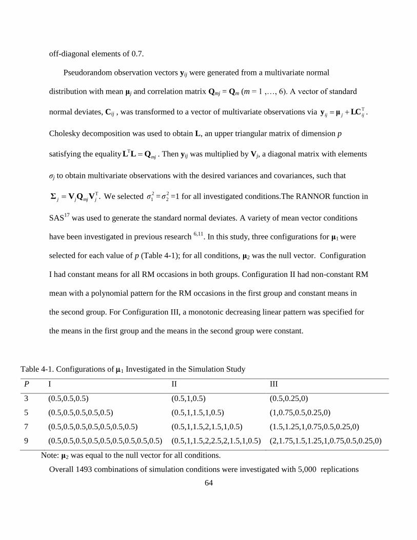
64

off-diagonal elements of 0.7.

Pseudorandom observation vectors yij were generated from a multivariate normal

distribution with mean μj and correlation matrix Qmj = Qm (m = 1 ,…, 6). A vector of standard

normal deviates, Cij , was transformed to a vector of multivariate observations via T

ijjij LCμy .

Cholesky decomposition was used to obtain L, an upper triangular matrix of dimension p

satisfying the equality mjQLL T. Then yij was multiplied by Vj, a diagonal matrix with elements

σj to obtain multivariate observations with the desired variances and covariances, such that

.T

jmjjj VQVΣ We selected 2

1σ =2

2σ =1 for all investigated conditions.The RANNOR function in

SAS17

was used to generate the standard normal deviates. A variety of mean vector conditions

have been investigated in previous research 6,11

. In this study, three configurations for μ1 were

selected for each value of p (Table 4-1); for all conditions, μ2 was the null vector. Configuration

I had constant means for all RM occasions in both groups. Configuration II had non-constant RM

mean with a polynomial pattern for the RM occasions in the first group and constant means in

the second group. For Configuration III, a monotonic decreasing linear pattern was specified for

the means in the first group and the means in the second group were constant.

Table 4-1. Configurations of 1 Investigated in the Simulation Study

P I II III

3 (0.5,0.5,0.5) (0.5,1,0.5) (0.5,0.25,0)

5 (0.5,0.5,0.5,0.5,0.5) (0.5,1,1.5,1,0.5) (1,0.75,0.5,0.25,0)

7 (0.5,0.5,0.5,0.5,0.5,0.5,0.5) (0.5,1,1.5,2,1.5,1,0.5) (1.5,1.25,1,0.75,0.5,0.25,0)

9 (0.5,0.5,0.5,0.5,0.5,0.5,0.5,0.5,0.5) (0.5,1,1.5,2,2.5,2,1.5,1,0.5) (2,1.75,1.5,1.25,1,0.75,0.5,0.25,0)

Note: μ2 was equal to the null vector for all conditions.

Overall 1493 combinations of simulation conditions were investigated with 5,000 replications

65

for each combination. The study was conducted using SAS/IML software17

. Two measures of

performance were used to evaluate the DFCs: mean square error (MSE) and norm of the average

bias18

. The former is

||)ˆ(1

||1

aa

M

k

kM

b , (12)

and the latter is

M

k

kM

e1

2||ˆ||1

aa , (13)

where a is the population vector of DFCs, ||x|| is the norm of x and M is the number of

replications (i.e., M = 5000). Both measures takes values on the interval [0, ) and the smaller

the bias or error in the DFCs, the better. To adjust for the confounding effect of degree of

separation between the two group means on bias and error, the MSE and bias in the DFCs were

standardized using the distance between the two group mean vectors. Therefore,

|||| 21 μμ

bbst

, (14)

and

|||| 21 μμ

eest

. (15)

4.4 Results

The average standardized MSE and bias values are summarized in Tables 4-2 to 4-5 for the

four investigated values of p.

As Table 4-2 reveals for p = 3, when the observations in both groups were sampled from

populations with constant mean vectors (i.e., configuration I), MSE was smallest (and similar)

66

for both the STCS and STAR DA procedures and largest for the UN procedure. When the data

were sampled from a population with a non-constant mean configuration (i.e., configurations II

or III), MSE and bias were smallest for either the UN or STCS procedure and were substantially

largest for the STUN and STAR procedures. For example, under a CS covariance structure and

when ρ = 0.7 and p = 3, the UN and STAR procedures had the smallest and largest average MSE,

respectively, when data were sampled from a population with mean configuration II, while the

UN and STUN procedures had the smallest and largest MSE respectively, when data were

sampled from a population with mean configuration III.

For DA procedures based on constant mean vectors (i.e., STUN, STCS, and STAR), the

average MSE decreased as the correlation among the RMs increased when the mean and

covariance structure were correctly specified. This finding was observed regardless of the

number of RMs. But when either the covariance or mean structure was misspecified, the average

MSE increased as the correlation among the repeated measurements increased. For example,

when p = 3 and under AR-1 population covariance structure, the average MSE for the UN

procedure was 0.35 and 0.64 when ρ = 0.3 and ρ = 0.7, respectively, while the average MSE of

the STAR procedure were 0.07 and 0.05 when ρ = 0.3 and ρ = 0.7, respectively, when data were

sampled from a population with constant mean configuration (Table 4-2).

For DA procedures based on structured covariances, the average MSE and bias increased

when the covariance structure was misspecified and the mean structures were correctly specified,

regardless of the number of RMs. For example, under a AR-1 population covariance structure

and when ρ = 0.3 and p = 3, the average MSE and bias of the STCS procedure were 1.3 and 2.0

times the average MSE of the STAR procedure, respectively, when the data were sampled from a

population with mean configuration I. Similarly, the average MSE and bias of DA procedures

67

based on structured covariances increased under a correctly specified population covariance but a

misspecified mean structure. For example, when p = 3 and ρ = 0.3 under AR-1 population

covariance structure, the average MSE and bias of the STAR procedure when the data were

sampled from a population with mean configuration II were 6.4 and 7.0 times the average MSE

and bias of the STAR procedure under a constant mean configuration, respectively.

For the STUN procedure, the average bias increased when the mean and covariance structures

were misspecified, but STCS procedure had the smallest MSE when the data were sampled from

a population with a constant mean configuration, regardless of the number of RM. For example,

when p = 7, under an unstructured population covariance structure and when ρ = 0.3 and p = 7,

the average MSE and bias of the STUN procedure were 0.70 and 2.75 times the average MSE

and bias of the STCS procedures, respectively, when the data were sampled from a population

with a constant mean configuration (Table 4-4).

Moreover, for each DA procedure, the average MSE and bias due to misspecification of

the covariance structure increased as the magnitude of correlation and number of RMs increased.

For example, when p = 5 and under a CS population covariance structure, the average MSEs of

the STAR procedure were 2.6 and 5.5 times the average MSE of the STCS procedure for ρ = 0.3

and ρ = 0.7, respectively, when data were sampled from a population with a constant mean

configuration (Table 3). The corresponding bias values for the STAR procedure were 4.2 and

10.7 times the bias of the STCS procedure when ρ = 0.3 and ρ = 0.7, respectively. Similarly,

when p = 9, the average MSEs of the STCS procedure were 8,3 and 11.0 times the average MSE

of the STAR procedure for ρ = 0.3 and ρ = 0.7, respectively, while the corresponding average

bias values were 11.0 times the average bias of the STCS procedure when ρ = 0.3 and ρ = 0.7

(Table 4-5).

68

Finally, analyses revealed that the average MSE for each of the DA procedures decreased

as the sample size increased. For example, the average MSEs of UN procedure were 7.82, 3.77,

and 2.50 when N = 60, 90, and 120 respectively. In contrast, the average bias for each DA

procedure remained largely unchanged as the sample size increased, regardless of the mean

configuration and number of RM. For example, the overall average bias of the STAR procedure

were 2.12, 2.10 and 2.10 when N = 60, 90, and 120, respectively.

69

Table 4-2. Average Standardized MSE and Bias by Covariance Structure, Magnitude of Correlation, and Mean Configuration for p = 3

Covariance Structure

ρ Mean Configuration

MSE Bias

UN STUN STCS STAR UN STUN STCS STAR CS 0.3 I 0.34 0.11 0.07 0.09 0.08 0.08 0.07 0.15 II 0.31 0.45 0.38 0.52 0.09 0..52 0.52 0.61 III 0.52 0.64 0.61 0.63 0.13 0.98 0.98 0.98 0.7 I 0.65 0.12 0.05 0.09 0.06 0.05 0.05 0.21 II 0.65 1.89 1.81 2.38 0.14 1.20 1.20 1.38 III 1.16 3.00 2.95 2.99 0.25 2.27 2.27 2.29 AR(1) 0.3 I 0.35 0.14 0.09 0.07 0.08 0.08 0.15 0.08 II 0.30 0.56 0.33 0.44 0.09 0.59 0.47 0.56 III 0.48 0.43 0.41 0.41 0.11 0.75 0.77 0.75 0.7 I 0.64 0.13 0.08 0.05 0.06 0.06 0.22 0.06 II 0.66 3.29 2.44 3.10 0.16 1.61 1.40 1.58 III 1.01 1.11 1.06 1.06 0.16 1.34 1.36 1.34 UN 0.3 I 0.38 0.13 0.08 0.16 0.08 0.08 0.15 0.27 II 0.34 0.33 0.41 0.53 0.10 0.42 0.54 0.60 III 0.61 1.20 1.25 1.31 0.18 1.40 1.45 1.47 0.7 I 0.67 0.12 0.05 0.12 0.06 0.05 0.08 0.27 II 0.66 1.47 1.52 2.03 0.13 1.05 1.10 1.27 III 1.29 4.34 4.41 4.48 0.32 2.77 2.81 2.83

Note: See Table 4-1 for a description of the mean configurations; CS = compound symmetric; AR-1 = first-order autoregressive; UN =

unstructured; ρ = correlation parameter; UN = unstructured mean and covariance; STUN = structured mean and unstructured

covariance; STCS = structured mean and CS covariance; STAR = structured mean and AR-1 covariance. Numbers in bold correspond to

bias and error values of DA procedures for which the mean and covariance structures are correctly specified.

70

Table 4-3. Average Standardized MSE and Bias by Covariance Structure, Magnitude of Correlation and Mean Configuration for p = 5



MSE Bias

UN STUN STCS STAR UN STUN STCS STAR CS 0.3 I 0.56 0.14 0.05 0.13 0.06 0.06 0.05 0.21 II 0.53 0.96 0.80 1.09 0.09 0.60 0.60 0.69 III 0.63 1.21 1.13 1.16 0.12 0.89 0.89 0.91 0.7 I 1.10 0.16 0.02 0.11 0.04 0.04 0.03 0.23 II 1.35 4.40 4.19 5.20 0.18 1.39 1.39 1.54 III 1.80 6.06 5.95 6.00 0.27 2.08 2.08 2.09 AR(1) 0.3 I 0.56 0.20 0.08 0.05 0.09 0.09 0.14 0.07 II 0.46 0.76 0.37 0.48 0.09 0.48 0.38 0.45 III 0.55 0.57 0.47 0.45 0.10 0.55 0.56 0.55 0.7 I 1.06 0.21 0.08 0.04 0.05 0.05 0.22 0.04 II 0.96 2.42 1.51 2.01 0.11 0.99 0.83 0.95 III 1.08 0.86 0.76 0.72 0.10 0.72 0.74 0.72 UN 0.3 I 0.66 0.20 0.14 0.20 0.08 0.08 0.31 0.35 II 0.64 2.26 1.33 1.67 0.11 0.96 0.77 0.86 III 0.75 1.61 1.63 1.61 0.15 1.03 1.08 1.07 0.7 I 1.15 0.17 0.03 0.10 0.04 0.03 0.07 0.22 II 1.40 4.81 4.44 5.35 0.18 1.45 1.42 1.56 III 2.04 7.57 7.66 7.76 0.30 2.33 2.36 2.37

Note: See Table 4-1 for a description of the mean configurations; CS = compound symmetric; AR-1 = first-order autoregressive; UN

= unstructured; ρ = correlation parameter; UN = unstructured mean and covariance; STUN = structured mean and unstructured

covariance; STCS = structured mean and CS covariance; STAR = structured mean and AR-1 covariance. Numbers in bold correspond

to bias and error values of DA procedures for which the mean and covariance structures are correctly specified

71

Table 4-4. Average Standardized MSE and Bias by Covariance Structure, Magnitude of Correlation and Mean Configuration for p = 9



MSE Bias

UN STUN STCS STAR UN STUN STCS STAR CS 0.3 I 1.33 0.31 0.03 0.25 0.07 0.07 0.03 0.33 II 1.54 2.56 2.04 2.51 0.13 0.66 0.66 0.74 III 1.64 2.88 2.53 2.59 0.16 0.84 0.84 0.85 0.7 I 2.18 0.29 0.01 0.11 0.03 0.03 0.02 0.22 II 5.14 11.58 10.97 12.40 0.29 1.54 1.54 1.64 III 6.12 14.07 13.66 13.72 0.37 1.96 1.96 1.96 AR(1) 0.3 I 1.19 0.47 0.07 0.04 0.12 0.12 0.13 0.07 II 0.98 1.41 0.51 0.75 0.09 0.41 0.31 0.40 III 1.40 1.38 0.74 0.78 0.13 0.44 0.44 0.47 0.7 I 2.17 0.46 0.07 0.02 0.07 0.07 0.19 0.03 II 2.05 2.51 0.86 1.22 0.09 0.58 0.43 0.51 III 2.03 1.27 0.69 0.70 0.10 0.41 0.43 0.41 UN 0.3 I 1.95 0.47 0.09 0.33 0.08 0.07 0.22 0.41 II 4.73 10.85 12.28 12.84 0.32 1.46 1.63 1.67 III 6.85 35.01 30.47 30.74 0.43 2.40 2.26 2.27 0.7 I 2.86 0.37 0.01 0.12 0.04 0.03 0.06 0.23 II 8.52 24.32 23.45 25.40 0.43 2.26 2.25 2.35 III 10.07 32.21 31.44 32.00 0.56 2.98 2.97 2.99

Note: See Table 4-1 for a description of the mean configurations; CS = compound symmetric; AR-1 = first-order autoregressive; UN =

unstructured; ρ = correlation parameter; UN = unstructured mean and covariance; STUN = structured mean and unstructured

covariance; STCS = structured mean and CS covariance; STAR = structured mean and AR-1 covariance; Numbers in bold correspond

to bias and error values of DA procedures for which the mean and covariance structures are correctly specified.

72

4.5 Conclusions

This manuscript investigated the effects of RM mean and/or covariance structure mis-

specification on bias and error in DFCs for DA procedures based on parsimonious mean and/or

covariance structures. As expected, the bias and error in the DFCs of the investigated procedures

increased when the RM mean and/or covariance structures were misspecified. The average bias

and error variation due to misspecification of the RM mean structure was greater than the

average bias and error variation due to RM covariance structure misspecification for all of the

investigated procedures. While DA procedures based on parsimonious RM mean and covariance

structures had negligible bias when the mean and covariances are correctly specified, the UN DA

procedure had the smallest bias when the data were sampled from a population with non-constant

mean configuration.

Based on the study findings, we recommend adopting a DA procedure based on

unstructured mean vectors and covariance matrices when the researcher has prior knowledge to

suggest that the mean longitudinal profile for each group will change across the repeated

measures occasions. If the mean longitudinal profile in each group is not expected to increase or

decrease across the measurement occasions, either the STCS or STAR procedure are

recommended because they require estimation of a fewer number of parameters, although any of

the procedures can be expected to perform well in terms of both bias and error variation.

To reduce the effect of mean and/or covariance structure misspecification on bias and

error in the DFCs, preliminary tests of model fit could be undertaken before adopting a DDA

procedure for RM data. Graphical exploration of the data, likelihood ratio tests, or penalized log-

likelihood measures like the Akaike information criterion have all been proposed to guide the

73

specification of mean and covariance structures19

.

The limitations of this study should be noted. We focused on normally distributed data. The

impact of mean and/or covariance misspecification on bias and error in the DFCs when data are

sampled from non-normal distribution has not been investigated. While mild departures from

multivariate non-normality are known to have little effect on classification accuracy of

conventional DA procedure20

, classification accuracy can be severely affected under large

departures21-22

. Inferences about DFCs of the linear DA procedures may also be affected by the

degree of departure from the assumption of multivariate normality22

. The DA procedures

considered in manuscript also focused only on complete data, an assumption which may not be

satisfied in RM studies, which are often characterized by missing observations and unbalanced

measurements occasions23

. In the simulation study, the RM variances were assumed to be

constant across variables and groups. Linear DA procedures rest on the assumption of covariance

homogeneity2. Departures from this assumption may result in reduced classification accuracy

24.

DFCs have been shown to be relatively robust to violation of this assumption when the data are

normally distributed25

, but it is not known if this robustness will continue to be evident when the

covariance and/or mean vector is misspecified.

A number of opportunities for future research exist in the development of DDA procedures

for RM data. Although several studies have examined the effects of population distribution on

classification accuracy, there is limited investigation of the effects of population distribution and

other data characteristics on bias and error in DFCs. Existing studies in this area have only

focused on the effects of sample size, number of outcome variables, and mean configuration on

bias and variation in DFCs when data were sampled from normally distributed data12, 26

. This

study investigated DA procedures based on constant mean vectors and/or structured covariances.

74

However, the assumption of a constant repeated measures group mean structure may not be

tenable when the interest is in the assessment of the relative importance of measurement

occasions that discriminate between groups. DA procedures based on non-constant mean vectors

and CS or AR-1 covariance structures can be further investigated. These procedures which

assume non-constant mean configurations and parsimonious structures will be useful for

assessing the relative importance of information collected at each measurement occasions in

univariate repeated measures studies.

In summary, although the adoption of a DA procedure based on a parsimonious mean and/or

covariance structure can reduce the number of parameters to estimate, which is beneficial when

sample size is small6, this study shows that bias and error variation in the DFCs can be large,

particularly when there is misspecification of the RM mean structure. A researcher’s choice of a

DA procedure for RM data is dependent, in part, on the trade-off between parsimony in

parameter estimation and bias and/or error in the DFCs.

75

Acknowledgements

This research was supported by a Canadian Institutes of Health Research (CIHR) Vanier

Graduate Scholarship to the first author, and a CIHR New Investigator Award to the second

author.

76

References


of Eugenics, 7, 179 – 188.

2. Huberty, C. J., & Olejnik, S. (2006). Applied MANOVA and Discriminant Analysis. New

York: Wiley.

3. Feighner, J. P., & Sverdlov, L. (2002). The use of discriminant analysis to separate a

study population by treatment subgroups in a clinical trial with a new pentapeptide

antidepressant. Journal of Applied Research, 2, 17 – 18.

4. Levesque, L., Ducharme, F., Zarit, S. H., Lachance, L., & Giroux, F. (2008). Predicting

longitudinal patterns of psychological distress in older husband caregivers: further

analysis of existing data. Aging Mental Health, 12, 333 – 343.

5. Marshall, G., & Baron, A. E. (2000). Linear discriminant models for unbalanced

longitudinal data. Statistics in Medicine, 19, 1969 – 1981.







with temporal autocorrelation. Advances in Data Analysis and Classification, 1, 175 –

199.


77


10. Thomas, D. R. (1992). Interpreting discriminant functions: a data analytic approach.

Multivariate Behavioral Research, 27, 335 – 362.

11. William, B. K., & Titus, K. (1988). Assessment of sampling stability in ecological


12. William, B. K., Titus, K., & Hines, J. E. (1991). Stability and bias of classification rates

in biological applications of discriminant analysis. The Journal of Wildlife Management,

54, 331 – 341.


discrimination – The effects of distributional properties. Statistics in Medicine, 10, 757 –

766.

14. He, X., & Fung, W. K. (2000). High breakdown estimation for multiple populations with

applications to discriminant analysis. Journal of Multivariate Analysis, 72, 151 – 162.

15. Lei, P., & Koehly, L. M. (2003). Linear discriminant analysis versus logistic regression: a

comparison of classification errors in the two-group case. Journal of Experimental

Education, 72, 25 – 49.

16. Thomas, D. R., & Zumbo, B. D. (1996). Using a measure of variable importance to

investigate the standardization of discriminant coefficients. Journal of Educational and

Behavioral Statistics, 21, 110 – 130.

17. SAS Institute Inc. (2008). SAS/IML user's guide, version 9.2. Cary, NC: SAS Institute,

Inc.

18. Croux, C., & Dehon, C. (2001). Robust linear discriminant analysis using S-estimators.

Canadian Journal of Statistics, 29, 473 – 493.

78

19. Fitzmaurice, G., Laird, N. M., & Ware, J. H. (2004). Applied Longitudinal Analysis. New

Jersey: Wiley.

20. Ashikaga, T., & Chang, P. C. (1981). Robustness of Fisher’s linear discriminant function

under two-component mixed-normal models. Journal of the American Statistical

Association, 76, 375 – 676.

21. Lachenbruch, P. A., Sneeringer, C., & Revo, L. T. (1973). Robustness of the linear and

quadratic discriminant function to certain types of non-normality. Communications in

Statistics, 1, 39 – 57.

22. McLachlan, G. J. (1992). Discriminant Analysis and Statistical Pattern Recognition.

New York: Wiley.

23. Fairclough, D. L., Peterson, H. F., Cella, D., & Bonomi, P. (1998). Comparison of several

model-based methods for analysing incomplete quality of life data in cancer clinical

trials. Statistics in Medicine, 17, 781 – 796.

24. Solberg, H. E., 1988. Discriminant analysis. Critical Reviews in Clinical Laboratory

Sciences, 9, 209 – 242.

25. Owen, J. G., & Chmielewski, M. A. (1985). On canonical variates analysis and the

construction of confidence ellipses in systematic studies. Systematic Zoology, 34, 366 –

374.

79

Appendix I: Maximum Likelihood Estimation for RMDA Procedures

For DDA with constant mean structure, let Θ be a column vector of model parameters,

where the first two elements denote the mean parameters and the last two elements correspond to

σ2 and ρ, respectively. Let ijy be 1 p vector of repeated measurements on the ith participant (i

= 1, 2…., nj, j = 1, 2; N = n1 + n2) in the jth group, and Yj denote the njp data matrix for the jth

group. Then the log of the joint likelihood function L is

)},()({tr2

1||log

22log

2) ,...,,|log( 1

2

1 1

T

21 jij

j

n

i

jijN

jNNpy μyΣμyΣyy Θ

(A-1)

where T is the transpose operator.

Assuming a constant mean structure for the group means,

pjj c 1μ , (A-2)

where cj is the mean for the measurement occasions for the jth group and 1p is a p 1 vector of

ones). Equation 4 in the text simplifies to

),)()((tr2

1

)(tr2

1||log

22log

2),|log(

2

1

1

1

21

j

pjjpjjj ccn

NNp

1yΣ1y

WΣΣYYΘ

(A-3)

where W = W1 + W2, ,)()( T

1

jij

n

i

jijj

j

yyyyW

and tr is the trace operator. Equating the first

order derivatives of equation A-3 to zero, the ML estimate of the mean values for the jth group,

cj is as given in equation 4.

Assuming a CS covariance structure forjΣ ,

Σ = ])1[( T2

ppp 11I , (A-4)

80

where is the magnitude of correlation among the repeated measurements, 2 is repeated

measures variance assumed to be constant across measurement occasions, and Ip is the pp

identity matrix. Then,

|Σ| = ,)1]()1(1[ 12 pp p (A-5)

and

],)1(1

[)1(

1 T

2

1

pppp

11IΣ

(A-6)

where Σ is positive definite, and 11

1

p. Substituting the values of |Σ| and Σ

-1 in

equations A-4 and A-5 into the log of the likelihood function (equation A-2) gives

),(tr)1(1

)()1(2

1

)1log(2

)1())1(1log(

2log

22log

2

2

2

JWW

ptr

pNp

NNNp

(A-7)

where W is as defined in equation 7, and J is a p ×p

matrix of ones. The first order derivatives of

the log-likelihood function with respect to σ2 and ρ are as given in equations 5 and 6 The

maximum likelihood (ML) estimates of σ2 and ρ are obtained by setting f1 and f2 to zero and

solving the equations. The ML estimates of the DFCs for this DDA procedure are obtained by

substituting the ML estimates of cj , σ2 , and ρ into equation 1.

81

DDA based on Constant Means and AR-1 Covariance Structure

Assuming a first-order autoregressive structure forΣ ,

122 )1(|| pp Σ , (A-8)

12

1-

)1(

p 2

0ΣΣ , (A-9)

where

10....00

10....00

....................

0....10

0....01

00....01

2

2

2

0Σ

. (A-10)

The first order derivatives of the log of the joint likelihood function of equation A-2 is given in

equation 8. Here,

pm

jp

j

y1T

1 , (A-11)

)2(

1

T

2

pm

jpjjp

j

yyy1, (A-12)

and 1j

y and jp

y , are respectively, the first and pth elements of the vector j

y

Substituting the values of |Σ| and Σ-1

from equations A-8 and A-9 into the log-likelihood

function (equation A-2) gives

))1(

tr(2

1)1log(

2

)1(log

22log

2 22

022 *W

Σ

pNNpNp, (A-13)

where

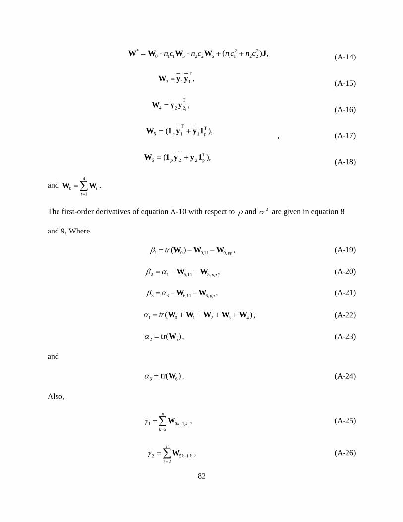
82

,)( -- 2

22

2

116225110

*JWWWW cncncncn

(A-14)

,

T

113 yyW (A-15)

,

T

224 1yyW

(A-16)

),( T

p1

T

15 1yy1W p , (A-17)

),( T

p2

T

26 1yy1W p (A-18)

and

4

1

0

t

tWW .

The first-order derivatives of equation A-10 with respect to and 2 are given in equation 8

and 9, Where

pptr ,011,001 )( WWW , (A-19)

pp,511,512 WW , (A-20)

pp,611,633 WW , (A-21)

)( 432101 WWWWW tr , (A-22)

)(tr 52 W , (A-23)

and

)(tr 63 W . (A-24)

Also,

p

k

kk

2

,101 W , (A-25)

p

k

kk

2

,152 W , (A-26)

83

and

,2

,163

p

k

kkW (A-27)

where Wuk-1,k is the (k-1,k)th element of Wu (u = 0 ,…, 6) and k = 1 ,…, p. The ML estimates of

c1, c2, σ2 and ρ are obtained by solving the systems of equations 8, 9, and 10 simultaneously. The

ML estimates of the vector of DFCs for this DDA procedure is obtained by substituting the ML

estimates of c1, c2, σ2, and ρ into equation 1.

84

Section II: Robust Discriminant Analysis for Non-Normal Data

85

Chapter 5. Discriminant Analysis for Non-normal Data

Abbreviations

CT = Coordinatewise trimming




HRQOL = Health-related quality of life

MCD = Minimum covariance determinant

MER = Misclassification error rates



MVE = Minimum volume ellipsoid



TL = Trimmed likelihood

86

5.1 Introduction

The previous section examines discriminant analysis (DA) procedures that assume

parsimonious covariance and mean structures for normally distributed repeated measures data1-3

.

However, these DA procedures rest on the assumptions of multivariate normality and covariance

homogeneity, which may not be satisfied in practice. Normality of the outcome variables may

not be a tenable assumption in clinical investigations. For example, patient-reported outcomes

such as health-related quality of life measures frequently exhibit heavy-tails and skewed

distributions4. Also, treatment groups may exhibit greater variability than control groups

5-6.

The linear DA procedure will sometimes result in smaller misclassification error rates

(MERs) for predictive discriminant analysis (PDA) in multivariate non-normal than normal

data7-9

. It may also frequently produce incorrect variable rankings for descriptive discriminant

analysis (DDA) when the data are non-normal10

. Although several DA procedures that are

insensitive (i.e., robust) to departures from multivariate normality assumptions in multivariate

group designs, there are limited investigations about robust DDA procedures for rank ordering

variables in non-normal data. Also, robust repeated measures discriminant analysis (RMDA)

procedures for describing group separations in non-normal repeated measures data have not been

developed.

This chapter reviews the literature on robust DA procedures for multivariate data and repeated

measures data.

5.2 Robust Discriminant Analysis for Multivariate Group Designs

DA classification procedures that are robust to departures from multivariate normal distributions

87

have been developed for predicting group memberships in multivariate group designs. These

include (a) DA procedures based on rank transformation of the data, and (b) DA procedures

based on robust estimators of means and covariances. The former includes procedures based on

rank transformation of the data11

, rank cut-offs12

, and non-linear transformation of the data13

.

While these procedures have been shown to improve classification accuracy5, DA based on

transformation of the non-normal data may not be appropriate when there are between-group

interactions because the ranks are not a linear function of the original scores14-15

.

DA procedures based on robust estimators of means and covariance matrices have been

proposed for predicting group memberships in non-normal data. The robustness of an estimator

is typically quantified via the breakdown point, the minimum proportion of outliers in the data

that can inflate the estimators arbitrarily far from their true values. The breakdown point for least

squares estimators is zero16

. Among the robust estimators of means and covariance is the class of

M-estimators of mean and covariance which was first proposed by Huber17

. In M-estimators, a

weighted function of the Mahalanobis distances (M-distances) of the observations is applied to

the data such that observations with large M- distances are given reduced weights while

observations with smaller M-distances are given larger weights. DA procedures based on M-

estimators of mean and covariances have been shown to improve classification accuracy than the

conventional DA based on least squares estimators when data are non-normal18

. Campbell19-20

also proposed robust DA coefficients based on M-estimators applied to canonical scores of the

data. However, DA procedures based on M-estimators have low breakdown points as the data

dimension increases21

.

DA procedures have also been developed based on robust estimators with high breakdown

points for classification in non-normal multivariate data. This includes S-estimators22-23

,

88

minimum covariance determinant (MCD) estimators, and minimum volume ellipsoid (MVE)

estimators24

. In MCD and MVE estimators, the means and covariance estimates are obtained

from a subset of the data with the smallest covariance determinant or volume ellipsoid. Robust

DA procedures based on MCD or MVE estimators are obtained by replacing the conventional

least squares estimates with the MCD or MVE estimates of the mean and covariances,

respectively. However, these procedures may be computationally intensive for high-dimensional

multivariate data and may not result in improved classification accuracy when there are no

outliers in the data22

.

DA procedures have been developed based on trimmed estimators, for which means and

covariance estimates are computed based on a subset of the original data obtained by removing a

predetermined proportion of the observations from each tail of the distribution of the original

data. The trimming approach, which was first developed for testing differences between group

means when data are non-normal and group covariances are homogeneous, are intuitively

appealing estimators because of their computational simplicity and good theoretical properties25

.

Ahmed and Lachenbruch26

proposed robust DA procedures based on applying DA to a subset of

the original data obtained by removing observations with extreme Mahalanobis scores. This

includes a DA procedure based on the iterative trimming suggestion of Gnanadesikan and

Kettenring27

in which 5% or 10% of the observations with the largest Mahalanobis distances are

trimmed, and the classification rule is developed based on the mean and covariance estimates of

the remaining observations. Another approach uses a classification rule developed from a subset

of the original data obtained by trimming the discriminant scores of the observations. These

robust DA procedures showed better classification accuracy than the classical DA based on least

squares estimators in non-normal data. However, Campbell19

notes that the former and latter DA

89

procedures may not achieve the optimal classification accuracy in non-normal data because the

Mahalalnobis scores of the observations is influenced by the outliers.

5.2 Trimmed Estimation in Multivariate and Repeated Measures Data

Tukey & McLaughlin28

first proposed trimmed estimators based on the Student t test for testing

differences between population means. Let 1)(Y )2(Y …. )nY( denote the order statistics for

a random sample of size n drawn from a population with a continuous symmetric distribution

function F(( )

Y) and unknown mean μ and standard deviation σ. Define gj = [δn], where δ

represents the proportion of the observations to be trimmed, or censored, from each tail of the

distribution and [x] is the integer less than or equal to x. Then the δ-trimmed mean is

gn

Y

Y

gn

gi

i

t

2

1

. (1)

This trimmed mean has been shown to asymptotically follow a normal distribution by the

following theorem.

Theorem: Univariate Trimming

For a continuous symmetric population with distribution function F, let denote the

quantile, i.e., F( ) = . As n ,

))(,0(N)( 2 tYn , (2)

where

1

2)()21()( 222 tdFt .

Tukey & Mclaughlin26

were the first to Studentize trimmed means. They proposed the

trimmed t statistic

90

)1(/(

~2

hhs

Yt

w

t , (3)

where 2

ws is the Winsorized sums of squared deviations, and h = n – 2g is the effective number of

observations.

Other variants of this test statistic have been developed including Yuen’s t-statistic29-30

.

Wilcox31

proposed the Winsorized variance as a consistent estimator of the variance of the

trimmed data instead of the trimmed variance data when testing for differences between

population means for non-normal data. He showed that test procedures based on trimmed means

and Winsorized variances are more robust to the effects of variance heterogeneity and non-

normality than test procedures based on least squares estimators.

Several trimmed estimators of means and covariances have been developed for non-

normal multivariate data. We review a number of trimming approaches that has not previously

been used to develop robust DA procedures.

Srivasta and Mudholkar32

proposed an extension of univariate trimming to multivariate

data. This approach is based on coordinate trimming of the multivariate data to develop robust

estimators of means and covariance matrices.

Let Yi = (Yi1, Yi2,…, Yip)T (i = 1, …, n) denote an independent and identically distributed

random vector from a population with μ = (μ1 … μp)T and Σ , where

T is the transpose operator.

Let F(Y1 Y2,…, Yp) define the joint distribution function, Flk(Yl, Yk) denote the bivariate

distribution function for Yl, and Yk, and Fk(yk) (l, k = 1, 2,…., p) denote the marginal distribution

function for the kth variable. The parameters μ and Σ are estimated by T1 )(ˆ p2 Y ... Y Yμ and Σ ,

respectively. Let knkk YYY )((2)1) ....( denote the order statistic of the sample for the kth variable.

91

The trimmed mean Ttt1tt )(ˆ p2 Y , ... ,Y Yμ where

gn

gi

kik Ygn

Y1

)(t2

1 (4)

is the trimmed mean for the kth outcome variable, and g = [δn], where δ represents the

proportion of the observations to be trimmed, or censored, from each tail of the distribution and

[x] is the integer less than or equal to x. The trimmed mean has been shown to asymptotically

follow a multivariate normal distribution by the following theorem.

Theorem: Multivariate Coordinate Trimming32,33

Asymptotically, as n ,

).,()ˆ( )(wpt Nn Σ0μμ (5)

The Winsorized covariance has been shown as a consistent estimator of .)(wΣ The estimated

Winsorized covariance is

Sw= (sm), (6)

where

1

))((1

n

zzzz

s

lilm

n

i

im

m

j

, (7)

is the variance for the mth and lth outcome, and

n

i

imm zn

y1

w ,1

(8)

is the group winsorized mean for the mth outcome, where

mgim yz )1( if mgim yy )1(

92

= imy if mgnimmg yyy )()1( (9)

= mgny )( if mgnim yy )( , for i = 1, …, n. □

Robust estimators based on coordinatewise trimming (CT) of the data have been adopted in

previous studies for multivariate and repeated measures procedures. For example, Srivastava and

Mudholkar32

developed a robust Hottelling T2-statistic based on 15% coordinate-wise trimming

of the non-normal multivariate data. Keselman et al.34

proposed robust non-pooled Welch-type

and Huynh Improved General Approximation test statistics based on CT of the data for testing

main and interaction effects in repeated measures designs when data are non-normal.

Trimmed likelihood (TL) estimation is another approach that has been proposed for

obtaining robust estimates of means and covariances for likelihood-based models 35-36

but has not

been used to develop robust DA procedures for non-normal repeated measures data. Under this

approach, robust estimates of the mean and covariance are obtained by trimming the likelihood

function rather than directly trimming the data. The trimmed likelihood is expressed as

gn

i

gnfTL1

)()1( ),|,...,(),( ΣμyyΣμ . (10)

The robust estimates of the mean and covariance are obtained by maximizing the trimmed

likelihood function. Because the likelihood is scalar-valued, this trimming approach can be done

on univariate as well as multivariate data. However, in elliptical distributions, the maximum

trimmed likelihood approach is equivalent to trimming the Mahalanobis distance as suggested by

Ahmed and Lachenrbuch27

, which may not be efficient due to the distortion of the sample mean

and covariance matrices.

Another general class of trimmed estimators for likelihood-based models adopts two-stage

93

trimming, in which initial robust estimation (e.g., trimming, MCD or MVE) are used to select a

sub-sample of the data prior on which likelihood-based inferences are made. Previous work in

this area includes the two-stage robust estimator of Broffit, Clarke, and Lachenbruch37

in which a

proportion of observations with the largest Mahalanobis distance are trimmed prior to

maximization of the likelihood function. Cuesta-Albertos, Matran, and Mayo-Iscar38

also

suggested an iterative two-stage method in which the robust estimation is used to obtain a

suitably trimmed dataset on which ML estimation is conducted. This approach has been shown

to result in high-breakdown estimators of means and covariances when data are non-normal,

however, its extension to discriminant analysis have not been investigated.

5.3 Discussion

This chapter reviews existing robust DA procedures that have been developed for non-

normal data. This includes DA procedures based on rank transformation of the non-normal data

and other computer-intensive empirical methods for developing robust estimators. More

specifically, trimmed estimation methods for multivariate group designs and repeated measures

data, which are computationally efficient with good asymptotic properties, are reviewed.

This chapter reviews a number of other trimmed estimation approaches that has not been

previously investigated for developing robust DA procedures. While all these approaches have

been shown to be robust to non-normality, the choice among these robust estimation approaches

remains unclear as there are no previous investigations comparing these estimation methods.

While CT estimation method is not as computationally intensive as other robust methods, it is

less sensitive to outlying observations because observations considered to be an outlier based on

one variable but not an outlier on the other variables are not necessarily removed from the data.

94

For RMDA procedures that are developed for repeated measures data, there are no previous

investigations of robust RMDA procedures for non-normal repeated measures data. Although the

existing robust DA procedures for multivariate group designs can be extended to repeated

measures data, they do not take advantage of the special structure in the data and may be not be

useful for describing group separation in high dimensional non-normal data. While previous

research has shown that the bias and error in the DFCs of the conventional DA procedures have

been, there is limited investigation of the effects of non-normality on the bias and error in

discriminant function coefficients (DFCs) of the conventional DA and RMDA procedures that

assume parsimonious covariance structures. These procedures are useful for evaluating the

relative importance of variables in longitudinal studies such as health-related quality of life

(HRQOL) studies that are often characterized by non-normal distributions.

The RMDA procedures that assume constant means have been described in the previous

chapters. These procedures have been shown to improve the accuracy of the classification rule

for repeated measures data and advantageous when the sample size is small relative to the

number of repeated measures data. However, the assumption of constant repeated measures

mean may not be tenable in longitudinal studies that investigate longitudinal changes on one or

more variables over time. For example, in longitudinal studies of growth or maturation processes

in groups of children or adolescents, the assumption of constant group means may not be tenable

when the interest is in describing the differences in the longitudinal profiles of groups39-40

. In the

next chapter, we propose new RMDA procedures that assume unstructured group means and

parsimonious covariance structures. Also robust RMDA procedures that assume parsimonious

means and/or covariance structures are developed for describing group separation in non-normal

repeated measures data.

95

Despite the benefits of adopting DA procedures based on robust estimators, one limitation

of robust estimators is increased bias in the parameter estimates as the breakdown point

increases41

. Our goal in developing robust RMDA procedures is to derive robust DFCs with

smaller bias and errors that can be used to describe group separation in non-normal repeated

measures data. In the next chapter, we investigate the influence of population distribution on bias

and error of DFCs of the robust RMDA procedures under a variety of data analytic conditions in


96

References







with temporal autocorrelation. Advances in Data Analysis and Classification, 1, 175 -

199.

4. Beaumont, J. L., Lix, L. M., Yost, K. J., & Hahn, E. A. (2006). Application of robust

statistical methods for sensitivity analysis of health-related quality of life outcomes.

Quality of Life Research, 15, 349 – 356.

5. Blair, R.C., & Sawilowsky, S. (1993). Comparison of two tests useful in situations where

treatment is expected to increase variability relative to controls. Statistics in Medicine,

12, 2233 – 2243.

6. Troendle, J.F., Blair, R.C., Rumsey, D., & Moke, P. (1997). Parametric and non-

parametric tests or the overall comparison of several treatments to a control when

treatment is expected to increase variability. Statistics in Medicine, 16, 2729 – 2739.



766.



97


9. Lachenbruch, P. A., Sneeringer, C, & Revo, L. T. (1973). Robustness of the linear and

quadratic discriminant function to certain types of non-non-normality. Communications

in Statistics, 1, 39 – 57.


York: Wiley.

11. Conover, W. J., & Iman, R. L. (1980). The rank transformation as a method of

discrimination with some examples. Communications in Statistics, 9, 465 – 487.

12. Randles, R. H., Broffit, J. D., Ramberg, J. S., & Hogg, R. V. (1978a). Discriminant

analysis based on ranks. Journal of the American Statistical Association, 73, 379 – 384.

13. Velilla, S., & Barrio, J. A. (1994). A discriminant rule under transformation.

Technometrics, 36, 348 – 353.

14. Blair, R. C., Sawilowsky, S. S., & Higgins, J. J. (1987). Limitations of the rank transform

statistic in tests for interactions. Journal of Communications in Statistics – Simulation &

Computation, 16, 1133 – 1145.

15. Sawilowsky, S. S., Blair, R. C., & Higgins, J. J. (1989). An investigation of the type I

error and power properties of the rank transform procedure in factorial ANOVA. Journal

of Educational Statistics, 14, 255 – 267.

16. Chork, C. Y., & Rousseeuw, P. J. (1992). Integrating a high breakdown option into

discriminant analysis in exploration geochemistry. Journal of Geochemical Exploration,

43, 191 – 203.

17. Huber, P. J. (1964). Robust Estimation for a location parameter. Annals of Mathematical


98

18. Randles, R. H., Broffit, J. D., Ramberg, J. S., & Hogg, R. V. (1978b). Generalized linear

and quadratic discriminant functions using robust estimates. Journal of the American

Statistical Association, 73, 564 – 568.

19. Campbell, N. A. (1979). Canonical variate anlaysis: some practical aspects. PhD Thesis,

University of London.

20. Campbell, N. A. (1982). Robust procedures in multivariate analysis II. Robust canonical

variate analysis. Applied Statistics, 31, 1 – 8.

21. Hawkins, D. M., & McLachlan, G. J. (1997). High-breakdown linear discriminant

analysis. Journal of the American Statistical Association, 92, 136 – 143.


applications to discriminant analysis. Journal of multivariate analysis, 72, 151 – 162.



24. Roussew, P.J., & van Zomeren, B. C. (1990). Unmasking multivariate outliers and

leverage points. Journal of American Statistical Association, 85, 633 – 661.

25. Wilcox, R. R. (1994). Some results on the Tukey-McLaughlin and Yuen methods for

trimmed means when distributions are skewed. Biometrical Journal, 36, 259 – 273.

26. Ahmed, S. W., & Lachenbruch, P. A. (1977). Discriminant analysis when scale

contamination is present in the initial sample. In Classification and Clustering; J.Van

Ryzin, ed, 331 – 353. New York, Academic Press.

27. Gnanadesikan, R., & Kettenring, J. R. (1972). Robust estimates, residual, and other

outliers detection with multiresponse data. Biometrics, 28, 81 – 124.

28. Tukey, J. W., & McLaughlin, D. H. (1963). Less vunelrable confidence and significance

99

procedures for location based on a single sample: trimming/winsorization I. Sankhya A,

25, 331 – 352.

29. Yuen, K. K. (1974). The two-sampled trimmed t for unequal population variances.

Biometrika, 61, 165 – 170.

30. Dixon, W. J., & Yuen, K. K. (1974). Trimming and winsorization: A review. Statistical

Papers, 15, 157 – 170.

31. Wilcox, R. R. (1995). ANOVA: A paradigm for low power and misleading measures of

effect size. Review of Educational Research, 65, 51 – 77.

32. Srivastava, D. K., & Mudholkar, G. S. (2001). Trimmed T2: A robust analog of

hottelling’s T2. Journal of Statistical Planning and Inference, 97, 343 – 358.

33. Arcones, M. A. (1995). Asymptotic normality of multivariate trimmed means. Statistics

& Probability Letters, 25, 43 – 53.

34. Keselman, H. J., Kowalchuk, R. K., Algina, J., Lix, L., & Wilcox, R. R. (2000). Testing

treatment effects in repeated measures designs: trimmed means and bootstrapping. British

Journal of Mathematical and Statistical Psychology, 53, 175 – 191.

35. Bednarski, T., & Clarke, B. R. (1993). Trimmed likelihood estimation of location and

scale of the normal distribution. Australian Journal of Statistics, 35, 141 – 153.

36. Hadi, A. S., & Luceno, A. (1997). Maximum trimmed likelihood estimators: a unified

approach, examples, and algorithms. Computational Statistics & Data Analysis, 25, 251 –

272.

37. Broffit, B., Clarke, W. R., & Lachenbruch, P. A. (1980). The effects of Huberizing and

trimming on the discriminating function. Communications in Statistics A- Theory and

Methods, 9, 13 – 25.

100

38. Cuesta-Albertos, J. A., Matran, C., & Mayo-Iscar, A. (2008). Trimming and likelihood:

Robust location and dispersion estimation in the elliptical model. Annals of Statistics, 36,

2284 – 2318.



40. Groenink, M., Rozendaal, L., Naeff, M. S. J., et al. (1998). Marfan syndrome in children

and adolescents: predictive and prognostic value of aortic root growth for screening for

aortic complications. Heart, 80, 163 – 169.

41. Daszykowski, M., Kaczmarek, K., Vander Heyden, Y., & Walczak, B. (2007). Robust

statistics in data analysis – a review of Basic Concepts. Chemometrics and Intelligent

Laboratory Systems, 85, 203 – 219.

101

Chapter 6. Robust Descriptive Discriminant Analysis for Repeated Measures Data

Tolulope T. Sajobi1

Lisa M. Lix1, 3

Bolanle M. Dansu1,2

William Laverty3

Longhai, Li3

1School of Public Health, University of Saskatchewan, Saskatoon, CANADA

2Department of Statistics, University of Agriculture, Abeokuta, NIGERA

3Department of Mathematics & Statistics, University of Saskatchewan, Saskatoon, CANADA

The manuscript presented in this chapter has been accepted for publication in Computational

Statistics and Data Analysis. It has been re-organized in this chapter to meet the dissertation

requirements of the University of Saskatchewan. The candidate’s contributions include the

development of new robust descriptive discriminant analysis procedures, design and

implementation of Monte Carlo study, statistical analysis of the example dataset, and preparation

of the published manuscript

102

Abbreviations

AR-1 = First-order autogressive structure

CS = Compound symmetric structure




DFC = Discriminant function coefficients

HT-I = Non-normal distribution with moderately heavy tails

HT-II = Non-normal distribution with extremely heavy tails


MER = Misclassification error rates


MVE = Minimum volume ellipsoid



RMSE = Root mean square error

SK-I = Non-normal distribution with moderate skewness

SK-II = Non-normal distribution with extreme skeweness

STAR = DA based on structured means and covariances with a AR-1 structure

STCS = DA based on structured means and covariances with a CS structure

UN = Unstructured


UNCS = DA based on unstructured means and covariances with a CS structure

103

UNAR = DA based on unstructured means and covariances with a AR-1 structure

104

Abstract

Discriminant analysis (DA) procedures based on parsimonious mean and/or covariance

structures have recently been proposed for repeated measures data. However, these procedures

rest on the assumption of a multivariate normal distribution. This study examines repeated

measures DA (RMDA) procedures based on maximum likelihood (ML) and coordinatewise

trimming (CT) estimation methods and investigates bias and root mean square error (RMSE) in

discriminant function coefficients (DFCs) using Monte Carlo techniques. Study parameters

include population distribution, covariance structure, sample size, mean configuration, and

number of repeated measurements. The results show that for ML estimation, bias in DFC

estimates was usually largest when then data were normally distributed, but there was no

consistent trend in RMSE. For non-normal distributions, the average bias of CT estimates for

procedures that assume unstructured group means and structured covariances was at least 40%

smaller than the values for corresponding procedures based on ML estimators. The average

RMSE for the former procedures was at least 10% smaller than the average RMSE for the latter

procedures, but only when the data were sampled from extremely skewed or heavy-tailed

distributions. This finding was observed even when the covariance and mean structures of the

RMDA procedure were mis-specified. The proposed robust procedures can be used to identify

measurement occasions that make the largest contribution to group separation when the data are

sampled from multivariate skewed or heavy-tailed distributions.

Key Words: bias; covariance structure; discriminant function coefficients; repeated

measurements; root mean square error

105

6.1. Introduction

Linear discriminant analysis (DA)1 is a multivariate procedure for predicting group

membership (predictive discriminant analysis; PDA) and/or describing group separation

(descriptive discriminant analysis; DDA) on a set of correlated variables. The former focuses on

the accuracy of classification while the latter uses discriminant function coefficients (DFCs) to

rank order variables according to their contributions to group separation2. The linear DA

procedure makes no assumptions about the structures of the means or covariances of the

variables other than the assumption of homoscedasticity (i.e., equality) of group covariances.

Recently, several repeated measures DA (RMDA) procedures based on parsimonious mean and

covariance structures, including constant means and compound symmetric (CS) or first-order

autoregressive (AR-1) covariances, have been developed for PDA3-6

. These procedures are

efficient when sample size is small relative to the number of repeated measurements, although

mis-specification of the mean or covariance structure may influence bias and accuracy.

Previous research has shown that while the linear DA procedure will sometimes result in

smaller misclassification error rates (MERs) for PDA in multivariate non-normal than normal

data7-9

, it will also frequently produce incorrect variable ranks for DDA when the data are non-

normal10

. Thus, departures from the assumption of multivariate normality may have serious

consequences for researchers who adopt the linear DA procedure. However, the effects of non-

normality on the performance of RMDA procedures based on parsimonious mean and covariance

structures have received little, if any, attention.

Several linear DA procedures that are robust (i.e., insensitive) to departures from the

assumption of multivariate normality have been proposed11-12

by replacing the conventional

least-squares estimators of means and covariances with robust estimators, including M-

106

estimators13

, S-estimators14,15

, minimum covariance determinant (MCD) estimators16-17

,

minimum volume ellipsoid (MVE) estimators17, 18

, and estimators based on the trimmed

Mahalanobis distance (M-distance)19,20

;. Some of these estimators have shown poor performance

for PDA. Specifically, M-estimators may result in high MERs in high-dimensional data21

.

Moreover, estimators based on trimmed M-distances may be sensitive to multivariate outliers13

One approach that has not previously been used to develop robust DA procedures is to adopt

estimators based on coordinatewise trimming (CT). In univariate data, trimmed means possess

good theoretical properties for heavy-tailed and skewed distributions, are computationally

efficient, and straightforward to implement22

. To implement CT, the coordinates of the

multivariate data are independently trimmed by removing a pre-determined proportion of the

observations from each tail of the distribution. Trimmed means and Winsorized covariances are

then computed from the CT data; the latter are the theoretically correct estimators of variance

corresponding to the trimmed mean. Robust estimators based on CT have been adopted in

previous studies about multivariate and repeated measures procedures23-25

.

RMDA procedures have a number of applications for describing group differences or

predicting group membership. de Coster, Leentjens, Lodder, and Verhey26

used DA to develop a

classification rule for stroke patients. Self-reported depression scores at one, three, six, and nine

months post stroke were used to discriminate between patients with and without a clinical

diagnosis of depression. RMDA procedures can also be used to identify the ages at which there

are significant differences between the growth curves of male and female adolescents27-28

.

In this study, we investigate robust RMDA procedures based on parsimonious means and/or

covariances in which the conventional maximum likelihood (ML) estimates of the means and

covariances are replaced by ML estimates of means and covariance parameters based on CT. The

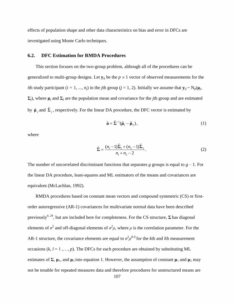
107

effects of population shape and other data characteristics on bias and error in DFCs are

investigated using Monte Carlo techniques.

6.2. DFC Estimation for RMDA Procedures

This section focuses on the two-group problem, although all of the procedures can be

generalized to multi-group designs. Let yij be the p 1 vector of observed measurements for the

ith study participant (i = 1, ..., nj) in the jth group (j = 1, 2). Initially we assume that yij ~ Np(μj,

Σj), where μj and Σj are the population mean and covariance for the jth group and are estimated

by jμ and jΣ , respectively. For the linear DA procedure, the DFC vector is estimated by

)ˆˆ(ˆˆ21

1μμΣa , (1)

where

.2

ˆ)1(ˆ)1(ˆ

21

2211

nn

nn ΣΣΣ (2)

The number of uncorrelated discriminant functions that separates g groups is equal to g – 1. For

the linear DA procedure, least-squares and ML estimators of the means and covariances are

equivalent (McLachlan, 1992).

RMDA procedures based on constant mean vectors and compound symmetric (CS) or first-

order autoregressive (AR-1) covariances for multivariate normal data have been described

previously4, 29

, but are included here for completeness. For the CS structure, Σ has diagonal

elements of σ2 and off-diagonal elements of σ

2ρ, where ρ is the correlation parameter. For the

AR-1 structure, the covariance elements are equal to σ2ρ

|k-l| for the kth and lth measurement

occasions (k, l = 1 ,…, p). The DFCs for each procedure are obtained by substituting ML

estimates of Σ, μ1, and μ2 into equation 1. However, the assumption of constant μ1 and μ2 may

not be tenable for repeated measures data and therefore procedures for unstructured means are

108

developed next.

For a RMDA procedure that assumes a CS structure for Σ and unstructured means, let Θ be

a column vector of model parameters where the first 2p elements denote the mean parameters

and the last two elements correspond to σ2 and σ

2ρ, respectively. Let Yj denote the njp data

matrix for the jth group and n = n1 + n2. Then the joint log-likelihood function is

)}()({tr2

1||log

22log

2),|(log 1

2

1 1

T

21 jij

j

n

i

jij

jnnpl μyΣμyΣYYΘ

, (3)

where T is the transpose operator. The ML estimate of μj is jμ and the estimates of ρ and 2 are

obtained by solving

,0)())()1(1())1(1)(1( 9898

2 bbaappnp (4)

and

,0)1)1()((

))1(1)(()1)()1(1()1(

2

98

2

98

2

pbb

paapppn

(5)

where a8 = tr(W1), a9 = tr(W2), b8 = tr(JW1), b9 = tr(JW2), Wj = ),()(1

T

jij

n

i

jij

j

yyyy

and

j

n

i

ij

jn

j

1

y

y , (6)

T

pp11J , and 1p is a p × 1vector of ones. The DFCs are estimated by substituting the ML

estimates of ρ, σ2, and μj into equation 1. The Appendix provides further details.

For a RMDA procedure with an AR-1 structure for Σ and unstructured mean vectors, the

ML estimate of μj is defined previously and the estimates of ρ and σ2 are obtained by solving

02)1( 222 αργβρρσnp , (7)

109

and

,0)()1()1( 2232 pnpn (8)

where 2)(tr 10WΣ ,

11

11 ,)(tr

l mpl

lmpp

,

WWWW , )(Wtrα ,

W = W1 + W2, and Wij is the (i, j)th element of W. The DFC estimates are obtained by

substituting the ML estimates of Σ (based on ρ and σ2), μ1, and μ2 into equation 1. The Appendix

provides further details.

6. 3. CT Estimation of DFCs

For CT of repeated measurements, let jmnjmjm jyyy )((2)1) .... ( denote the order statistics

for the jth group and the mth (m = 1, …, p) occasion. Define gj = [δnj], where δ represents the

proportion of the observations to be trimmed, or censored, from each tail of the distribution and

[x] is the integer less than or equal to x. When symmetric trimming is adopted, so that the same

number of observations are removed from each tail of the distribution, the effective sample size

for the jth group is fj = nj – 2gj. The trimmed mean for the jth group on the mth occasion is

jj

j

gn

gi

jmi

j

jm yf

y1

)(t

1. (8)

Define zijm as

jmgijm jyz )1( if jmgijm j

yy )1(

= ijmy if jmgnijmjmg jjjyyy )()1(

= jmgn jjy )( if jmgnijm jj

yy )( .

Then

110

jn

i

ijm

j

jm zn

z1

w ,1

(9)

is the jth Winsorized mean for the mth occasion. The Winsorized sum of squared deviations for

the mth and lth occasions in the jth group is

))(( ww

1

w jlijljm

n

i

ijmjml zzzzssj

, (10)

and Swj= (sswjml) is the Winsorized sums of squares and cross product matrix. The pooled

Winsorized covariance is

221

w2w1w

ff

SSΣ . (11)

For the linear DA procedure, CT is used to define a subsample of observations; trimmed

means and Winsorized covariances are computed as described. Robust estimates of the DFCs of

procedures that assume unstructured or structured means and structured covariances are derived

by maximizing the likelihood of the CT data. More specifically, CT is used to define a

subsample of observations for which means and covariances are estimated by solving the

systems of equations defined previously. Given that CT estimators are derived by trimming each

coordinate22, 30 - 31

, they share similar robustness properties to univariate trimmed estimators.

6.4. Simulation Study

A Monte Carlo study was conducted to examine bias and error in DFCs for the following

procedures: (a) conventional DA procedure that assumes unstructured means and covariances

(UNUN), (b) RMDA procedure that assumes unstructured means and CS covariances (UNCS),

(c) RMDA procedure that assumes unstructured means and AR-1 covariances (UNAR), (d)

111

RMDA procedure that assumes structured (i.e., constant) means and CS covariances (STCS), and

(e) RMDA procedure that assumes structured means and AR-1 covariances (STAR). The DFCs

of each procedure were estimated using ML methods applied to the original and CT data.

The following conditions were investigated: (a) number of repeated measurements (p), (b)

total sample size (n), (c) group sizes, (d) pattern and magnitude of correlation among the

repeated measurements, (e) mean configuration, and (f) population distribution. All procedures

were investigated for two independent groups.

The number of repeated measurements was set at p = 3, 5, and 7. Previous studies about

RMDA procedures have considered p ranging from 3 to 104. Total sample sizes of n = 60, 100,

and 140 were investigated. Although previous simulation studies for RMDA procedures have

primarily focused on equal group sizes4-5

, unequal group sizes have also been shown to affect the

MER of DA procedures8, 14

, and may therefore influence bias and RMSE of DFCs. For n = 60,

the group sizes were ( 21,nn ) = (30, 30), (24, 36), and (15, 45). For n = 100, they were ( 21,nn ) =

(50, 50), (40, 60), and (25, 75). For n = 140, the group sizes were ( 21,nn ) = (70, 70), (56, 84) and

(35, 105). These group sizes, which represents small to large degrees of group size imbalance,

were chosen based on previous research8,15, 29, 32

(Baron, 1991; Sajobi et al., in press; Van Aelst

& Willems, 2010). For the unequal group size cases, the coefficient of group size variation

ranged from 0.2 to 0.533

(Lix & Fouladi, 2007).

Error in DFCs is known to be influenced by both the magnitude and pattern of correlation

amongst the observations34

(Thomas & Zumbo, 1996). Therefore, six correlation structures were

investigated: (a) Q1: CS with ρ = 0.3 (b) Q2: CS with ρ = 0.6, (c) Q3: AR-1 with ρ = 0.3, (d) Q4:

AR-1 with ρ = 0.6, (e) Q5: UN with average ρ = 0.6, and (f) Q6: UN with average ρ = 0.6.

The data were generated from multivariate normal and non-normal distributions. For the

112

former, the marginal skewness and kurtosis values are γ1 = 0 and γ2 = 0, respectively.

Pseudorandom observation vectors yij were generated from a multivariate distribution with mean

μj and correlation matrix Qsj = Qs (s = 1, … , 6). A p×1 vector of standard normal deviates, Cij,

was transformed to a vector of multivariate observations via ijjij LCμy . The Cholesky

decomposition was used to obtain L, an upper triangular matrix of dimension p satisfying the

equality sjQLL T. Then yij was multiplied by Vj, a diagonal matrix with elements σj, to obtain

multivariate observations with the desired variances and covariances such that .T

jsjjj VQVΣ For

all the investigated conditions, Σ1 = Σ2.

When the assumption of multivariate normality was violated, we considered conditions in

which the data from the two groups were sampled from the same distribution as well as

conditions in which the data for the two groups were sampled from different distributions. For

the former, we considered two skewed distributions with γ1 = 1.8 and γ2 = 5.9 (SK-I) and γ1 =

13.2 and γ2 = 42892.9 (SK-II), respectively. Two heavy-tailed distributions were investigated,

with γ1 = 0 and γ2 = 33 (HT-I) for the first while the second was similar to a heavy-tailed Cauchy

distribution for which 1 and 2 are undefined (HT-II). For the latter, we investigated the case in

which observations in group 1 were sampled from a HT-II distribution while the observations in

group 2 were sampled from a SK-II distribution and denoted this condition by HT-II/SK-II.

These non-normal distributions represent moderate and extreme departures from multivariate

normality and have been investigated in previous studies employing trimmed estimators35, 36

(Berkovits, Hancock, & Nevitt, 2000; Keselman et al., 2007). Field and Genton37

describe a

family of multivariate non-normal distributions obtained by modifying the quantiles. The

variables g and h, which control the magnitude of γ1 and γ2, are used to transform a standard

normal variate, C, as follows:

113

2

2exp

)exp(ijm

ijm

ijm Ch

g

Cgy . (12)

When g = 0, this equation reduces to

ijmijmijm CCh

y )2

exp( 2 . (13)

The g and h parameters provide a convenient approach to generate data from multivariate

distributions. When g = h = 0, the distribution is multivariate normal. The parameter h

determines the heaviness of the tails of a distribution while the parameter g controls the

magnitude of skewness.

Three configurations for 1μ were selected based on previous research (Table 1) and

p1μ 5.02 for all conditions4, 38

. Configuration I had constant means across the repeated

measurements in both groups. Configuration II had non-constant means in a quadratic pattern for

the first group. For configuration III, a monotonic decreasing linear pattern was specified for 1μ .

These configurations represent the types of structures common in repeated measures studies39

.

Table 6-1. Configurations of μ1 for the Monte Carlo Study

Configuration p = 3 p = 5 p = 7

I (1, 1, 1) (1, 1, 1, 1, 1) (1, 1, 1, 1, 1, 1, 1)

II (1, 1.5, 1) (1, 1.5, 2, 1.5, 1) (1, 1.5, 2, 2.5, 2, 1.5, 1)

III (1, 0.75, 0.5) (1.5, 1.25, 1, 0.75, 0.5) (2, 1.75, 1.5, 1.25, 1, 0.75, 0.5)

Note: μ2 = 0.51p for all conditions.

For the robust procedures, a 20% symmetric trimming rule was adopted as recommended by

Wilcox22

. All combinations of conditions were investigated for each procedure and each method

of estimation, resulting in a total of 3 x 3 x 3 x 6 x 3 x 6= 2916 combinations. There were 10,000

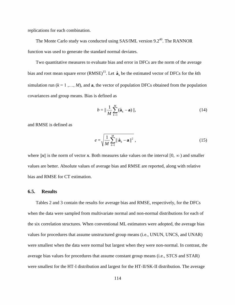
114

replications for each combination.

The Monte Carlo study was conducted using SAS/IML version 9.240

. The RANNOR

function was used to generate the standard normal deviates.

Two quantitative measures to evaluate bias and error in DFCs are the norm of the average

bias and root mean square error (RMSE)15

. Let ka be the estimated vector of DFCs for the kth

simulation run (k = 1 ,…, M), and a, the vector of population DFCs obtained from the population

covariances and group means. Bias is defined as

b = || )ˆ(1

1

aa

M

k

kM

||, (14)

and RMSE is defined as

e =

M

k

kM 1

2||ˆ||1

aa , (15)

where ||x|| is the norm of vector x. Both measures take values on the interval [0, ) and smaller

values are better. Absolute values of average bias and RMSE are reported, along with relative

bias and RMSE for CT estimation.

6.5. Results

Tables 2 and 3 contain the results for average bias and RMSE, respectively, for the DFCs

when the data were sampled from multivariate normal and non-normal distributions for each of

the six correlation structures. When conventional ML estimators were adopted, the average bias

values for procedures that assume unstructured group means (i.e., UNUN, UNCS, and UNAR)

were smallest when the data were normal but largest when they were non-normal. In contrast, the

average bias values for procedures that assume constant group means (i.e., STCS and STAR)

were smallest for the HT-I distribution and largest for the HT-II/SK-II distribution. The average

115

bias values for the investigated procedures based on ML estimators were sometimes influenced

by the correlation structure. For the UNUN procedure, average bias values were similar across

the six correlation structures. For all the procedures based on ML estimators, the average bias

was smallest for a CS or AR-1 correlation structure and largest for a UN structure (i.e, Q5 or Q6).

When CT estimation was adopted, average bias values for the UNUN, UNCS, and UNAR

procedures were smallest for the SK-I distribution and largest for the HT-II/SK-II condition. In

contrast, the average bias values for the STCS and STAR procedures were smallest when the

data were sampled from the SK-II distribution and largest for the normal distribution. For the

UNUN, UNCS and UNAR procedures, average bias was smallest for either a CS (i.e., Q1 and

Q2) or AR-1 (i.e., Q3 and Q4) structure. For the STCS and STAR procedures, bias was smallest

for the Q2 and Q3 structures but largest for the Q5 and Q6 structures, regardless of the population

distribution.

When the data were sampled from multivariate non-normal distributions, average bias

values were generally lower for robust than ML estimators. However, this depended on the

procedure and the correlation structure. For example, for the SK-I distribution with Q6, average

bias for the UNCS procedure based on ML and CT estimators were 0.45 and 0.32, respectively,

whereas the average bias values for the STCS procedure were 1.29 and 1.41, respectively. The

average bias values for UNUN, UNCS, and UNAR procedure based on CT estimators exhibited

smaller variability (i.e., standard deviation) than the corresponding ML estimates, although this

again depends on the covariance structure and population distribution. In contrast, the average

bias values for the STCS and STAR procedures based on ML estimators had larger standard

deviation values than those of the corresponding procedures based on ML estimators when data

were normal but not under non-normal distributions.

116

Table 6-2. Mean(SD) Bias of Discriminant Function Coefficients by Population Distribution and Correlation Structure

Distribution Correlation

Structure

ML Estimation CT Estimation

UNUN UNCS UNAR STCS STAR UNUN UNCS UNAR STCS STAR

Normal Q1 0.05(0.05) 0.06(0.05) 0.28(0.16) 0.75(0.33) 0.78(0.33) 0.13(0.07) 0.11(0.05) 0.32(0.14) 0.89(0.30) 0.90(0.29)

Q2 0.04(0.04) 0.04(0.05) 0.05(0.05) 0.34(0.25) 0.33(0.25) 0.18(0.06) 0.15(0.05) 0.15(0.05) 0.46(0.20) 0.43(0.20)

Q3 0.05(0.05) 0.16(0.06) 0.06(0.05) 0.51(0.21) 0.51(0.23) 0.13(0.05) 0.22(0.08) 0.11(0.05) 0.66(0.18) 0.64(0.19)

Q4 0.06(0.06) 0.35(0.14) 0.08(0.06) 0.87(0.29) 0.86(0.43) 0.11(0.05) 0.40(0.19) 0.09(0.04) 1.00(0.26) 0.98(0.38)

Q5 0.06(0.05) 0.54(0.34) 0.67(0.42) 1.04(0.55) 1.06(0.53) 0.14(0.06) 0.51(0.32) 0.68(0.40) 1.15(0.52) 1.16(0.50)

Q6 0.07(0.05) 0.32(0.13) 0.70(0.43) 1.39(0.67) 1.54(0.67) 0.18(0.12) 0.31(0.14) 0.69(0.38) 1.51(0.63) 1.65(0.63)

SK-I Q1 0.19(0.06) 0.22(0.06) 0.34(0.16) 0.64(0.38) 0.68(0.36) 0.08(0.04) 0.07(0.05) 0.28(0.16) 0.80(0.32) 0.83(0.31)

Q2 0.19(0.06) 0.22(0.05) 0.23(0.05) 0.38(0.18) 0.38(0.18) 0.10(0.05) 0.08(0.04) 0.07(0.04) 0.40(0.22) 0.38(0.22)

Q3 0.18(0.06) 0.23(0.06) 0.21(0.06) 0.43(0.22) 0.41(0.28) 0.07(0.04) 0.17(0.07) 0.06(0.04) 0.58(0.19) 0.57(0.21)

Q4 0.21(0.07) 0.37(0.08) 0.24(0.06) 0.77(0.30) 0.74(0.47) 0.08(0.04) 0.35(0.15) 0.07(0.06) 0.90(0.28) 0.89(0.41)

Q5 0.23(0.06) 0.62(0.33) 0.71(0.42) 0.97(0.56) 1.00(0.54) 0.13(0.08) 0.52(0.34) 0.66(0.42) 1.08(0.54) 1.10(0.52)

Q6 0.26(0.08) 0.45(0.18) 0.77(0.47) 1.29(0.72) 1.44(0.71) 0.11(0.05) 0.32(0.14) 0.70(0.43) 1.41(0.66) 1.56(0.67)

SK-II Q1 0.65(0.11) 0.72(0.12) 0.74(0.14) 0.74(0.21) 0.76(0.21) 0.34(0.06) 0.36(0.08) 0.45(0.14) 0.58(0.39) 0.66(0.36)

Q2 0.72(0.06) 0.81(0.04) 0.81(0.04) 0.78(0.04) 0.78(0.04) 0.23(0.09) 0.28(0.09) 0.28(0.09) 0.39(0.17) 0.40(0.17)

Q3 0.63(0.08) 0.69(0.06) 0.70(0.06) 0.66(0.10) 0.67(0.09) 0.30(0.07) 0.34(0.08) 0.34(0.08) 0.42(0.21) 0.43(0.25)

Q4 0.68(0.13) 0.73(0.13) 0.74(0.13) 0.78(0.21) 0.80(0.24) 0.37(0.10) 0.46(0.07) 0.43(0.09) 0.71(0.30) 0.69(0.45)

Q5 0.84(0.21) 1.02(0.34) 1.03(0.37) 1.05(0.42) 1.06(0.42) 0.51(0.19) 0.72(0.34) 0.78(0.41) 0.95(0.54) 0.98(0.52)

Q6 0.95(0.37) 1.09(0.46) 1.18(0.54) 1.26(0.65) 1.30(0.65) 0.66(0.24) 0.72(0.32) 0.92(0.51) 1.21(0.76) 1.34(0.74)

HT-I Q1 0.33(0.07) 0.36(0.07) 0.43(0.16) 0.58(0.39) 0.64(0.37) 0.10(0.06) 0.10(0.08) 0.28(0.17) 0.73(0.34) 0.77(0.33)

Q2 0.34(0.06) 0.38(0.06) 0.38(0.06) 0.45(0.13) 0.46(0.13) 0.06(0.05) 0.06(0.06) 0.06(0.06) 0.35(0.24) 0.34(0.24)

Q3 0.31(0.07) 0.34(0.07) 0.34(0.06) 0.42(0.20) 0.43(0.23) 0.07(0.05) 0.17(0.06) 0.09(0.07) 0.51(0.20) 0.51(0.24)

117

Q4 0.35(0.08) 0.43(0.06) 0.37(0.08) 0.72(0.31) 0.68(0.48) 0.14(0.06) 0.35(0.11) 0.16(0.07) 0.83(0.29) 0.82(0.44)

Q5 0.41(0.09) 0.72(0.33) 0.78(0.41) 0.95(0.54) 0.97(0.53) 0.20(0.12) 0.56(0.34) 0.67(0.43) 1.03(0.55) 1.05(0.52)

Q6 0.46(0.15) 0.60(0.24) 0.86(0.49) 1.22(0.76) 1.37(0.73) 0.24(0.07) 0.39(0.18) 0.74(0.47) 1.35(0.69) 1.49(0.69)

HT-II Q1 0.45(0.09) 0.51(0.09) 0.55(0.15) 0.62(0.32) 0.65(0.32) 0.19(0.07) 0.20(008) 0.33(0.16) 0.66(0.37) 0.71(0.36)

Q2 0.48(0.06) 0.55(0.05) 0.55(0.05) 0.56(0.05) 0.57(0.09) 0.09(0.08) 0.13(0.08) 0.13(0.08) 0.34(0.23) 0.35(0.22)

Q3 0.43(0.08) 0.48(0.08) 0.49(0.07) 0.49(0.15) 0.50(0.16) 0.15(0.07) 0.22(0.07) 0.19(0.08) 0.45(0.22) 0.45(0.27)

Q4 0.47(0.10) 0.55(0.09) 0.53(0.10) 0.71(0.29) 0.72(0.38) 0.23(0.07) 0.38(0.08) 0.27(0.08) 0.77(0.31) 0.74(0.48)

Q5 0.57(0.13) 0.85(0.35) 0.89(0.41) 0.98(0.52) 1.00(0.51) 0.32(0.16) 0.63(0.36) 0.72(0.46) 0.99(0.58) 1.03(0.55)

Q6 0.64(0.23) 0.80(0.33) 0.98(0.51) 1.20(0.75) 1.31(0.72) 0.41(0.12) 0.51(0.23) 0.80(0.49) 1.28(0.73) 1.42(0.71)

HT-II/SK-II Q1 0.65(0.10) 0.72(0.08) 0.75(0.09) 0.84(0.16) 0.85(0.15) 0.33(0.10) 0.31(0.07) 0.41(0.13) 0.61(0.39) 0.68(0.37)

Q2 0.75(0.13) 0.84(0.09) 0.84(0.09) 0.83(0.12) 0.83(0.12) 0.17(0.08) 0.20(0.08) 0.20(0.07) 0.36(0.20) 0.37(0.19)

Q3 0.66(0.12) 0.72(0.10) 0.73(0.10) 0.75(0.15) 0.76(0.13) 0.24(0.05) 0.24(0.06) 0.26(0.06) 0.43(0.22) 0.42(0.28)

Q4 0.65(0.11) 0.71(0.10) 0.71(0.09) 0.88(0.16) 0.90(0.17) 0.41(0.14) 0.45(0.10) 0.37(0.08) 0.73(0.31) 0.69(0.48)

Q5 0.82(0.13) 1.01(0.29) 1.03(0.32) 1.12(0.38) 1.13(0.37) 0.54(0.26) 0.68(0.36) 0.75(0.43) 0.96(0.55) 0.99(0.53)

Q6 0.86(0.22) 1.00(0.34) 1.11(0.47) 1.33(0.57) 1.35(0.58) 0.74(0.07) 0.70(0.17) 0.90(0.45) 1.24(0.75) 1.38(0.73)

Note: Normal distribution has skewness (γ1) = 0 and kurtosis (γ2) = 0; SK-I has γ1 = 1.8 and γ2 = 5.9; SK-II has γ1 = 13.2 and γ2 =

42892.9; HT-I has γ1 = 0 and γ2 = 33; HT-II has γ1 = ∞ and γ2 = ∞. Q1 = CS with ρ = 0.3; Q2 = CS with ρ = 0.6; Q3 = AR-1 with ρ =

0.3; Q4 = AR-1 with ρ = 0.6; Q5 = UN with average ρ = 0.3; Q6 = UN with average ρ = 0.6. ρ = correlation parameter. UNUN = UN

group means and UN covariances; UNCS = UN group means and CS covariances; UNAR = UN group means and AR-1 covariances;

STCS = Structured group mean vectors and CS-covariance structure; STAR = Structured group mean vectors and AR-1 covariance.

AR-1 = First-order autoregressive; CS = compound symmetric; UN = unstructured; SD = Standard deviation

118

Table 6-3. Average (SD) RMSE of Discriminant Function Coefficients by Population Distribution and Correlation Structure

Distribution Correlation

Structure



Normal Q1 0.55(0.17) 0.47(0.17) 0.55(0.12) 0.77(0.34) 0.80(0.33) 0.69(0.18) 0.57(0.18) 0.64(0.12) 0.91(0.31) 0.92(0.30)

Q2 0.42(0.l2) 0.34(0.13) 0.33(0.13) 0.36(0.25) 0.36(0.25) 0.55(0.12) 0.44(0.12) 0.44(0.13) 0.48(0.22) 0.45(0.21)

Q3 0.52(0.14) 0.44(0.13) 0.43(0.15) 0.53(0.23) 0.53(0.25) 0.65(0.15) 0.55(0.13) 0.53(0.16) 0.68(0.20) 0.66(0.21)

Q4 0.78(0.24) 0.65(0.16) 0.67(0.23) 0.89(0.29) 0.88(0.43) 0.93(0.26) 0.78(0.17) 0.78(0.25) 1.03(0.27) 1.01(0.39)

Q5 0.59(0.20) 0.76(0.27) 0.83(0.35) 1.05(0.55) 1.08(0.53) 0.72(0.21) 0.81(0.23) 0.89(0.32) 1.17(0.52) 1.18(0.50)

Q6 0.83(0.35) 0.79(0.28) 1.12(0.31) 1.41(0.67) 1.56(0.66) 1.02(0.37) 0.89(0.32) 1.20(0.30) 1.54(0.62) 1.68(0.62)

SK-I Q1 0.58(0.15) 0.50(0.15) 0.57(0.12) 0.67(0.36) 0.72(0.35) 0.68(0.18) 0.56(0.19) 0.63(0.13) 0.84(0.32) 0.86(0.32)

Q2 0.46(0.11) 0.39(0.12) 0.39(0.13) 0.40(0.19) 0.40(0.19) 0.54(0.13) 0.41(0.14) 0.41(0.14) 0.42(0.24) 0.41(0.24)

Q3 0.55(0.13) 0.45(0.14) 0.47(0.14) 0.46(0.24) 0.46(0.27) 0.64(0.15) 0.52(0.14) 0.52(0.17) 0.61(0.22) 0.60(0.23)

Q4 0.78(0.21) 0.63(0.15) 0.68(0.20) 0.80(0.30) 0.79(0.44) 0.91(0.25) 0.73(0.17) 0.77(0.24) 0.94(0.28) 0.93(0.41)

Q5 0.63(0.17) 0.80(0.28) 0.86(0.36) 0.99(0.55) 1.02(0.53) 0.71(0.22) 0.81(0.25) 0.88(0.33) 1.11(0.53) 1.12(0.51)

Q6 0.86(0.27) 0.83(0.21) 1.15(0.32) 1.33(0.69) 1.47(0.69) 0.97(0.34) 0.87(0.29) 1.19(0.30) 1.46(0.64) 1.60(0.65)

SK-II Q1 0.76(0.09) 0.78(0.10) 0.79(0.13) 0.78(0.20) 0.79(0.20) 0.68(0.14) 0.62(0.15) 0.69(0.12) 0.68(0.32) 0.73(0.32)

Q2 0.79(0.06) 0.84(0.04) 0.85(0.04) 0.80(0.05) 0.80(0.05) 0.53(0.13) 0.47(0.15) 0.47(0.15) 0.43(0.19) 0.43(0.19)

Q3 0.73(0.08) 0.74(0.07) 0.75(0.07) 0.69(0.10) 0.70(0.10) 0.65(0.13) 0.56(0.14) 0.59(0.15) 0.48(0.22) 0.50(0.24)

Q4 0.86(0.10) 0.80(0.12) 0.83(0.11) 0.82(0.20) 0.83(0.23) 0.83(0.15) 0.71(0.14) 0.78(0.14) 0.78(0.27) 0.79(0.37)

Q5 0.95(0.19) 1.06(0.33) 1.07(0.35) 1.08(0.41) 1.09(0.41) 0.80(0.19) 0.90(0.28) 0.95(0.34) 1.00(0.51) 1.03(0.50)

Q6 1.14(0.28) 1.19(0.40) 1.28(0.48) 1.30(0.62) 1.34(0.62) 1.03(0.13) 1.01(0.17) 1.23(0.35) 1.30(0.68) 1.41(0.67)

HT-I Q1 0.61(0.13) 0.56(0.12) 0.61(0.12) 0.64(0.35) 0.68(0.35) 0.65(0.18) 0.56(0.19) 0.63(0.13) 0.78(0.33) 0.81(0.33)

119

Q2 0.52(0.10) 0.49(0.11) 0.49(0.11) 0.47(0.15) 0.48(0.15) 0.51(0.13) 0.40(0.15) 0.40(0.15) 0.39(0.25) 0.38(0.25)

Q3 0.58(0.12) 0.50(0.13) 0.53(0.13) 0.45(0.22) 0.47(0.24) 0.62(0.15) 0.51(0.15) 0.52(0.17) 0.55(0.23) 0.55(0.25)

Q4 0.79(0.17) 0.65(0.13) 0.71(0.16) 0.76(0.30) 0.76(0.42) 0.87(0.23) 0.71(0.17) 0.76(0.22) 0.88(0.29) 0.88(0.41)

Q5 0.69(0.14) 0.86(0.28) 0.90(0.36) 0.98(0.53) 1.00(0.52) 0.70(0.21) 0.83(0.26) 0.89(0.33) 1.06(0.54) 1.08(0.52)

Q6 0.90(0.18) 0.91(0.16) 1.18(0.34) 1.29(0.70) 1.42(0.69) 0.94(0.30) 0.88(0.25) 1.20(0.31) 1.40(0.66) 1.54(0.66)

HT-II Q1 0.68(0.10) 0.65(0.10) 0.68(0.12) 0.67(0.30) 0.71(0.29) 0.67(0.17) 0.58(0.18) 0.65(0.13) 0.72(0.34) 0.77(0.34)

Q2 0.63(0.09) 0.63(0.09) 0.64(0.09) 0.59(0.11) 0.60(0.11) 0.52(0.14) 0.42(0.16) 0.42(0.16) 0.39(0.24) 0.39(0.23)

Q3 0.65(0.10) 0.59(0.11) 0.62(0.11) 0.53(0.17) 0.55(0.18) 0.64(0.15) 0.52(0.16) 0.54(0.17) 0.51(0.24) 0.51(0.26)

Q4 0.84(0.12) 0.71(0.12) 0.76(0.11) 0.77(0.27) 0.78(0.35) 0.87(0.20) 0.70(0.16) 0.77(0.20) 0.83(0.30) 0.83(0.42)

Q5 0.80(0.13) 0.95(0.31) 0.98(0.38) 1.02(0.50) 1.04(0.49) 0.75(0.21) 0.87(0.27) 0.92(0.35) 1.04(0.56) 1.07(0.53)

Q6 1.01(0.13) 1.02(0.20) 1.22(0.38) 1.27(0.68) 1.37(0.67) 0.97(0.22) 0.92(0.20) 1.21(0.33) 1.35(0.68) 1.48(0.67)

HT-II/SK-II Q1 0.81(0.10) 0.81(0.09) 0.84(0.09) 0.92(0.15) 0.93(0.14) 0.65(0.14) 0.54(0.14) 0.62(0.10) 0.66(0.35) 0.71(0.34)

Q2 0.87(0.13) 0.90(0.11) 0.90(0.11) 0.88(0.14) 0.88(0.13) 0.48(0.10) 0.35(0.10) 0.35(0.10) 0.38(0.19) 0.38(0.19)

Q3 0.83(0.11) 0.80(0.11) 0.82(0.11) 0.82(0.16) 0.83(0.15) 0.59(0.10) 0.45(0.11) 0.48(0.11) 0.45(0.22) 0.46(0.26)

Q4 0.91(0.10) 0.81(0.12) 0.86(0.09) 0.96(0.15) 0.98(0.15) 0.82(0.17) 0.66(0.14) 0.71(0.14) 0.77(0.29) 0.77(0.41)

Q5 0.97(0.13) 1.08(0.27) 1.10(0.29) 1.19(0.35) 1.19(0.35) 0.79(0.26) 0.84(0.31) 0.89(0.37) 0.98(0.54) 1.01(0.52)

Q6 1.10(0.12) 1.14(0.26) 1.27(0.37) 1.40(0.53) 1.42(0.53) 1.02(0.13) 0.92(0.11) 1.17(0.31) 1.30(0.70) 1.43(0.69)

Note: Normal distribution has skewness (γ1) = 0 and kurtosis (γ2) = 0; SK-I has γ1 = 1.8 and γ2 = 5.9; SK-II has γ1 = 13.2 and γ2 = 42892.9; HT-I

has γ1 = 0 and γ2 = 33; HT-II has γ1 = ∞ and γ2 = ∞. Q1 = CS with ρ = 0.3; Q2 = CS with ρ = 0.6; Q3 = AR-1 with ρ = 0.3; Q4 = AR-1 with ρ = 0.6;

Q5 = UN with average ρ = 0.3; Q6 = UN with average ρ = 0.6. ρ = correlation parameter. UNUN = UN group means and UN covariances; UNCS =

UN group means and CS covariances; UNAR = UN group means and AR-1 covariances; STCS = Structured group mean vectors and CS-

covariance structure; STAR = Structured group mean vectors and AR-1 covariance. AR-1 = First-order autoregressive; CS = compound

symmetric; UN = unstructured; SD = Standard deviation

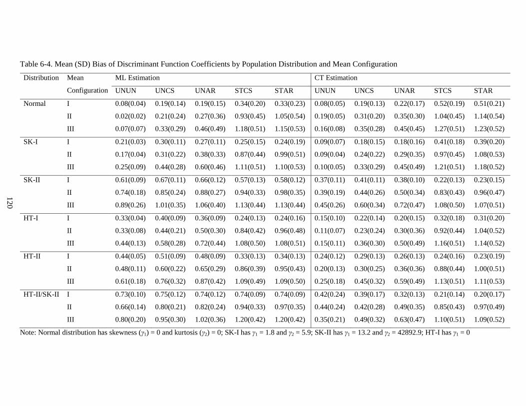
120

Table 6-4. Mean (SD) Bias of Discriminant Function Coefficients by Population Distribution and Mean Configuration

Distribution

Mean

Configuration



Normal I 0.08(0.04) 0.19(0.14) 0.19(0.15) 0.34(0.20) 0.33(0.23) 0.08(0.05) 0.19(0.13) 0.22(0.17) 0.52(0.19) 0.51(0.21)

II 0.02(0.02) 0.21(0.24) 0.27(0.36) 0.93(0.45) 1.05(0.54) 0.19(0.05) 0.31(0.20) 0.35(0.30) 1.04(0.45) 1.14(0.54)

III 0.07(0.07) 0.33(0.29) 0.46(0.49) 1.18(0.51) 1.15(0.53) 0.16(0.08) 0.35(0.28) 0.45(0.45) 1.27(0.51) 1.23(0.52)

SK-I I 0.21(0.03) 0.30(0.11) 0.27(0.11) 0.25(0.15) 0.24(0.19) 0.09(0.07) 0.18(0.15) 0.18(0.16) 0.41(0.18) 0.39(0.20)

II 0.17(0.04) 0.31(0.22) 0.38(0.33) 0.87(0.44) 0.99(0.51) 0.09(0.04) 0.24(0.22) 0.29(0.35) 0.97(0.45) 1.08(0.53)

III 0.25(0.09) 0.44(0.28) 0.60(0.46) 1.11(0.51) 1.10(0.53) 0.10(0.05) 0.33(0.29) 0.45(0.49) 1.21(0.51) 1.18(0.52)

SK-II I 0.61(0.09) 0.67(0.11) 0.66(0.12) 0.57(0.13) 0.58(0.12) 0.37(0.11) 0.41(0.11) 0.38(0.10) 0.22(0.13) 0.23(0.15)

II 0.74(0.18) 0.85(0.24) 0.88(0.27) 0.94(0.33) 0.98(0.35) 0.39(0.19) 0.44(0.26) 0.50(0.34) 0.83(0.43) 0.96(0.47)

III 0.89(0.26) 1.01(0.35) 1.06(0.40) 1.13(0.44) 1.13(0.44) 0.45(0.26) 0.60(0.34) 0.72(0.47) 1.08(0.50) 1.07(0.51)

HT-I I 0.33(0.04) 0.40(0.09) 0.36(0.09) 0.24(0.13) 0.24(0.16) 0.15(0.10) 0.22(0.14) 0.20(0.15) 0.32(0.18) 0.31(0.20)

II 0.33(0.08) 0.44(0.21) 0.50(0.30) 0.84(0.42) 0.96(0.48) 0.11(0.07) 0.23(0.24) 0.30(0.36) 0.92(0.44) 1.04(0.52)

III 0.44(0.13) 0.58(0.28) 0.72(0.44) 1.08(0.50) 1.08(0.51) 0.15(0.11) 0.36(0.30) 0.50(0.49) 1.16(0.51) 1.14(0.52)

HT-II I 0.44(0.05) 0.51(0.09) 0.48(0.09) 0.33(0.13) 0.34(0.13) 0.24(0.12) 0.29(0.13) 0.26(0.13) 0.24(0.16) 0.23(0.19)

II 0.48(0.11) 0.60(0.22) 0.65(0.29) 0.86(0.39) 0.95(0.43) 0.20(0.13) 0.30(0.25) 0.36(0.36) 0.88(0.44) 1.00(0.51)

III 0.61(0.18) 0.76(0.32) 0.87(0.42) 1.09(0.49) 1.09(0.50) 0.25(0.18) 0.45(0.32) 0.59(0.49) 1.13(0.51) 1.11(0.53)

HT-II/SK-II I 0.73(0.10) 0.75(0.12) 0.74(0.12) 0.74(0.09) 0.74(0.09) 0.42(0.24) 0.39(0.17) 0.32(0.13) 0.21(0.14) 0.20(0.17)

II 0.66(0.14) 0.80(0.21) 0.82(0.24) 0.94(0.33) 0.97(0.35) 0.44(0.24) 0.42(0.28) 0.49(0.35) 0.85(0.43) 0.97(0.49)

III 0.80(0.20) 0.95(0.30) 1.02(0.36) 1.20(0.42) 1.20(0.42) 0.35(0.21) 0.49(0.32) 0.63(0.47) 1.10(0.51) 1.09(0.52)

Note: Normal distribution has skewness (γ1) = 0 and kurtosis (γ2) = 0; SK-I has γ1 = 1.8 and γ2 = 5.9; SK-II has γ1 = 13.2 and γ2 = 42892.9; HT-I has γ1 = 0

121

and γ2 = 33; HT-II has γ1 = ∞ and γ2 = ∞. See Table 1 for a description of mean configurations. UNUN = UN group means and UN covariances; UNCS =

UN group means and CS covariances; UNAR = UN group means and AR-1 covariances; STCS = Structured group mean vectors and CS-covariance

structure; STAR = Structured group mean vectors and AR-1 covariance. AR-1 = First-order autoregressive; CS = compound symmetric; UN = unstructured;

SD = Standard deviation

122

Table 6-5. Mean (SD) RMSE of Discriminant Function Coefficients by Population Distribution and Mean Configuration

Distribution Mean

Configuration



Normal I 0.79(0.32) 0.70(0.27) 0.69(0.28) 0.36(0.20) 0.36(0.22) 0.95(0.35) 0.82(0.29) 0.82(0.30) 0.54(0.19) 0.53(0.21)

II 0.47(0.14) 0.42(0.20) 0.50(0.29) 0.93(0.45) 1.06(0.54) 0.61(0.16) 0.51(0.17) 0.58(0.26) 1.04(0.45) 1.14(0.54)

III 0.58(0.17) 0.59(0.24) 0.77(0.41) 1.21(0.51) 1.19(0.53) 0.73(0.18) 0.69(0.21) 0.84(0.38) 1.32(0.50) 1.28(0.53)

SK-I I 0.79(0.27) 0.70(0.22) 0.69(0.23) 0.30(0.15) 0.29(0.18) 0.93(0.32) 0.80(0.27) 0.79(0.28) 0.45(0.18) 0.43(0.21)

II 0.51(0.14) 0.46(0.20) 0.55(0.30) 0.87(0.44) 0.99(0.51) 0.59(0.16) 0.48(0.18) 0.56(0.28) 0.97(0.44) 1.09(0.53)

III 0.63(0.16) 0.64(0.26) 0.82(0.42) 1.15(0.51) 1.14(0.53) 0.70(0.17) 0.67(0.23) 0.85(0.40) 1.26(0.51) 1.24(0.53)

SK-II I 0.78(0.07) 0.75(0.08) 0.75(0.08) 0.62(0.11) 0.62(0.11) 0.84(0.19) 0.76(0.14) 0.75(0.16) 0.35(0.14) 0.35(0.15)

II 0.85(0.19) 0.89(0.24) 0.92(0.27) 0.95(0.33) 0.99(0.34) 0.67(0.20) 0.59(0.24) 0.67(0.32) 0.85(0.42) 0.97(0.47)

III 0.99(0.26) 1.06(0.35) 1.11(0.39) 1.16(0.43) 1.16(0.44) 0.76(0.22) 0.79(0.32) 0.94(0.42) 1.14(0.50) 1.13(0.51)

HT-I I 0.78(0.21) 0.71(0.16) 0.70(0.18) 0.32(0.12) 0.32(0.15) 0.89(0.29) 0.78(0.24) 0.77(0.26) 0.38(0.18) 0.37(0.20)

II 0.57(0.13) 0.55(0.21) 0.62(0.29) 0.85(0.42) 0.97(0.48) 0.57(0.16) 0.48(0.20) 0.57(0.30) 0.93(0.44) 1.05(0.52)

III 0.70(0.16) 0.73(0.28) 0.89(0.41) 1.13(0.50) 1.12(0.51) 0.68(0.17) 0.68(0.25) 0.86(0.41) 1.22(0.51) 1.20(0.52)

HT-II I 0.79(0.16) 0.73(0.10) 0.72(0.11) 0.42(0.10) 0.43(0.11) 0.88(0.26) 0.77(0.21) 0.76(0.23) 0.34(0.17) 0.34(0.19)

II 0.68(0.15) 0.68(0.22) 0.74(0.28) 0.87(0.39) 0.96(0.43) 0.61(0.18) 0.51(0.22) 0.60(0.32) 0.89(0.44) 1.01(0.50)

III 0.82(0.18) 0.87(0.21) 0.99(0.41) 1.14(0.49) 1.13(0.49) 0.72(0.18) 0.72(0.28) 0.89(0.42) 1.20(0.51) 1.18(0.52)

HT-II/SK-II I 0.96(0.08) 0.88(0.08) 0.89(0.07) 0.84(0.08) 0.84(0.08) 0.81(0.27) 0.67(0.22) 0.65(0.22) 0.29(0.15) 0.29(0.17)

II 0.84(0.15) 0.87(0.21) 0.90(0.24) 0.99(0.33) 1.02(0.34) 0.71(0.23) 0.56(0.26) 0.64(0.34) 0.86(0.43) 0.98(0.49)

III 0.94(0.18) 1.01(0.29) 1.10(0.35) 1.26(0.41) 1.25(0.41) 0.65(0.17) 0.65(0.29) 0.82(0.43) 1.12(0.51) 1.11(0.52)

Note: Normal distribution has skewness (γ1) = 0 and kurtosis (γ2) = 0; SK-I has γ1 = 1.8 and γ2 = 5.9; SK-II has γ1 = 13.2 and γ2 = 42892.9; HT-I has γ1 = 0

123

and γ2 = 33; HT-II has γ1 = ∞ and γ2 = ∞. See Table 1 for a description of mean configurations. UNUN = UN group means and UN covariances; UNCS =

UN group means and CS covariances; UNAR = UN group means and AR-1 covariances; STCS = Structured group mean vectors and CS-covariance

structure; STAR = Structured group mean vectors and AR-1 covariance. AR-1 = First-order autoregressive; CS = compound symmetric; UN = unstructured;

SD = Standard deviation

124

For RMSE, the bias values were consistently lowest for the UNUN, UNCS, and UNAR

procedures when ML estimators were adopted, but tended to be smaller for the normal

distribution than for non-normal distributions (Table 3). For the STCS and STAR procedures,

values were lower for non-normal than normal distributions. A comparison of procedures based

on ML and CT estimation revealed that when the data were normally distributed, the latter

procedures resulted in slightly higher average RMSE values than the former. RMSE was

generally lower for CT estimation than for ML estimation when the data were non-normal, but

again this depended on the procedure, the degree of departure from multivariate normality, and

the correlation structure.

Average bias and RMSE for each of the mean configurations and population distributions

are reported in Tables 4 and 5, respectively. For UNCS and UNAR procedures, the average bias

values (Table 4) were usually smaller for Configuration I, which had a constant mean pattern,

than for Configurations II and III, which had non-constant mean patterns, regardless of the

method of estimation and population distribution. For the STCS and STAR procedures, the

differences amongst the mean configurations were usually much larger. For example, the average

bias values for the STCS and STAR procedures under Configuration II were about 1.5 times the

values under Configuration I, when the data were sampled from the HT-II/SK-II distribution.

For CT estimation, average bias values for UNUN, UNCS, and UNAR procedures were

smaller than the values for the corresponding procedures based on ML estimators when the data

were sampled from non-normal distributions. For example, for Configuration III, the average

values for the UNAR procedure based on CT and ML estimators were 1.02 and 0.63,

respectively, for the SK-II/HT-II condition. For STCS and STAR procedures, the average bias

values were smaller for CT estimation than for ML estimation, but this again depended on the

125

mean configuration and the population distribution.

Moreover, the average RMSE values for STAR and STAR procedures (Table 5) were

smallest under Configuration I and largest under Configuration II or III, regardless of the

population distribution and estimation method. However, the average RMSE when the mean

structure was mis-specified increased for non-normal distributions. For example, the average

RMSE of the STCS procedure based on ML estimation for Configuration II was 2.6, 2.9, and 1.5

times greater than the average RMSE of the STCS procedure for Configuration I when data are

sampled from normal, SK-I, and SK-II distributions, respectively.

The average RMSE for the corresponding robust procedures were smaller than the

corresponding procedure based on ML estimators when the data were sampled from SK-II or

HT-II distributions but not the SK-I or HT-I distributions.

For robust UNUN, UNCS, and UNAR procedures, average RMSE values were smallest for

Configuration II and largest for Configuration I, regardless of the distribution. For

Configurations II and III, the average RMSE values for these procedures were smaller than the

corresponding procedures based on ML estimators when the data were sampled from a non-

normal distribution, except the SK-I distribution. Overall, the average RMSE values for

procedures based on CT estimators exhibited more variability than procedures based on ML

estimators.

Figure 1 provides average relative bias and RMSE for the procedures based on CT

estimation for non-normal distributions for different numbers of repeated measurements. While

the average relative bias for all the robust procedures increased with p, the average relative

RMSE values for these procedures remained largely unchanged for both skewed and heavy-

tailed distributions. But the average relative bias and RMSE for all the procedures increased as p

126

increased for the HT-II/SK-II distribution. Finally, the relative average bias and RMSE for

robust procedures that assume unstructured group means (i.e., UNUN, UNCS, and UNAR)

decreased as n increased when the data were sampled from non-normal distributions (Figure 2).

However, the change in average relative bias and RMSE for the robust procedures that assume

constant group means (i.e., STCS and STAR) was negligible as n increased.

127


Population Distributions and Number of Repeated Measurements

128


Population Distributions and Total Sample Size

129

6.6 Numeric Example

Data to illustrate the procedures are from the Manitoba Inflammatory Bowel Disease

(IBD) Cohort Study, a prospective longitudinal study, initiated in 2002, of patients recently

diagnosed with Crohn’s disease or ulcerative colitis41-42

. Data were collected at six-month

intervals using self-report instruments. Study participants were assigned to active (n1 = 265) and

inactive (n2 = 116) disease groups based on self-reported IBD symptoms at study entry.

Differences between active and inactive groups of participants on scores for a disease-specific

measure of quality of life, the IBD questionnaire (IBDQ), were investigated for the first two

years of the study (i.e., first five measurement occasions). The primary research question is

whether active and inactive disease groups differ in their longitudinal profiles of quality of life.

The group means and descriptive measures of skewness and kurtosis for a modified set of

IBDQ data are reported in Table 6. A mean imputation method was adopted to ensure complete

data at all occasions43

. Marginal measures of skewness and kurtosis suggest a moderate departure

from the assumption of a normal distribution in the active disease group when compared with the

inactive group (Table 6). A linearly increasing trend was observed (i.e., poorer quality of life)

for the active disease group, while a constant trend was observed for the inactive group. We use

the pooled covariance to estimate the DFCs (equation 2)

690.39

441.17677.50

379.60455.31795.76

05.35363.398487.39699.44

32.30914.29776.35072.384663.23

Σ .

The ML and robust estimates of the DFCs for each RMDA procedure are reported in Table

7. These were implemented using a SAS program written by the authors40

; the program is

provided in Appendix II. There are substantial differences in the estimated DFCs for the

130

procedures and for ML and robust estimation methods, leading to different conclusions about the

rank order of the repeated measurements for group discrimination. For the UNCS and UNAR

procedures, the CT estimates were larger than those of the UNCS procedure based on ML

estimators for all measurement occasions, except Month 18. For the UNUN procedure, the CT

estimates were larger than the ML estimates for Months 0, 18, and 24. In contrast, the CT

estimates for the STCS and STAR procedures were larger than the corresponding ML estimates

for the first three occasions.

Table 6-6. Descriptive Statistics for the Inflammatory Bowel Disease Questionnaire by Disease

Activity Group

Occasion

(Month)

Active Disease Group

Inactive Disease Group

Mean (SD) γ1 γ2 Mean (SD) γ1 γ2

0 158.37(27.94) 1.52 3.28 185.59(23.40) 0.97 2.28

6 165.53(28.53) 1.31 2.52 186.13(22.19) 0.34 -1.76

12 166.26(31.83) -1.73 4.40 188.27(18.76) -0.76 0.25

18 169.53(28.75) -0.98 1.06 188.60(19.82) -0.81 0.77

24 171.88(27.77) -1.98 5.70 188.09(23.25) -0.67 0.19

SD = Standard deviation; γ1 = skewness; γ2 = kurtosis

131

Table 6-7. Discriminant Function Coefficients for Discriminant Analysis Procedures Applied to

the Inflammatory Bowel Disease Questionnaire Data

Occasion (Month) UNUN UNCS UNAR STCS STAR

ML Estimation

0 -0.43 -0.22 -0.09 0.21 0.19

6 -0.29 -0.13 -0.17 0.15 0.07

12 0.30 0.69 1.00 0.59 0.30

18 0.43 0.56 0.28 0.54 0.28

24 0.10 0.43 0.32 0.55 0.53

CT Estimation

0 -0.69 -0.30 -0.13 0.29 0.28

6 0.10 -0.19 -0.23 0.21 0.11

12 0.24 0.74 1.06 0.63 0.33

18 0.56 0.46 0.20 0.47 0.25

24 0.19 0.45 0.38 0.51 0.49

UNUN = UN group means and UN covariances; UNCS = UN group means and CS covariances;

UNAR = UN group means and AR-1 covariances; STCS = Structured group means and CS-

covariance; STAR = Structured group means and AR-1 covariance. AR-1 = First-order

autoregressive; CS = compound symmetric; UN = unstructured

6.7 Discussion and Conclusions

In this study, we investigated RMDA procedures based on structured and unstructured

means and covariances with ML estimation and robust RMDA procedures based on CT and

illustrated their implementation using a numeric example. As expected, bias and error in the

DFCs of the investigated procedures were influenced by the shape of the population distribution,

but the effect of non-normality was associated with the population correlation structure and mean

configuration. Mis-specification of the mean and/or covariance structure resulted in increased

132

average bias and RMSE, but the effect was smaller when the data were multivariate non-normal

than when they were multivariate normal. Among all the investigated procedures, DA procedures

that assume unstructured group means and parsimonious covariance structures (i.e., UNCS and

UNAR) were less sensitive to mis-specification of the mean structure while the UNUN

procedure was least sensitive to mis-specification of the covariance structure regardless of the

population distribution.

As expected, RMDA procedures based on CT estimators were less sensitive to distribution

shape when compared to procedures based on ML estimation when the data were sampled from

non-normal distributions. More specifically, the DFCs of the UNCS and UNAR procedures

based on CT estimators were less biased and had less error than DFCs of other RMDA

procedures for extreme departures from a multivariate normal distribution. However, the DFCs

of these procedures may not always be more efficient than other procedures for moderate

departures from a multivariate normal distribution.

Based on the findings of this study, we recommend adopting a RMDA procedure based on

unstructured group means (i.e., UNUN, UNCS or UNAR) when the data are normally distributed

and their corresponding robust alternatives when there are indications of strong departure from

the multivariate normality assumption. However, the RMDA procedures based on CT estimators

may not be efficient in non-normal distributions when the group mean or covariance structure is

mis-specified. Therefore, we recommend that the choice among these RMDA procedures based

on unstructured group means should be guided by other data characteristics such as structure and

magnitude of correlations among the repeated measurements. A preliminary descriptive analysis

of the data could be undertaken to guide a researcher’s choice among these procedures. Also,

tests of model fit such as likelihood ratio tests, or penalized log-likelihood measures like the

133

Akaike information criterion might be used to guide the specification of mean and covariance

structures39

.

One criticism of CT estimators is that they rely on asymptotic normality of the trimmed

data25

and may be less efficient when the sample size is small and when data are normally

distributed22

. But as shown in the Monte Carlo study, the robust RMDA procedures that assume

no parsimony on the group means showed negligible differences in bias and RMSE for the

conventional and robust estimators under small sample size conditions and when the data were

normally distributed. Hence, they may be adopted by applied researchers when there are slight

departures from the assumption of multivariate normality.

This study has some limitations. The simulation study focused on conditions in which group

covariances were equal; this may not be a reasonable assumption in all data-analytic problems.

In addition, complete data were generated for all measurement occasions.

A number of opportunities exist in the development of robust RMDA procedures. While this

study showed that procedures based on trimmed estimators control bias and error under

departures from the multivariate normality assumption, further investigation about the effects of

population distribution on the ability of these procedures to correctly rank order repeated

measurements with respect to their relative contributions to group separation are needed44

.

Further research is needed to ascertain if reduction in bias and/or error in the DFCs of robust DA

procedures can lead to more accurate rank ordering of the repeated measurements under strong

departures from multivariate normality and other data-analytic conditions.

While RMDA procedures based on CT estimation controlled the bias in the DFCs when

the data were non-normal for correctly specified covariance and mean structures, the RMSE was

only controlled under the most extreme departures from non-normality. Therefore, while the

134

robust RMDA procedures investigated in this study show promise, further research is warranted

to investigate other approaches such as trimmed estimation methods based on robust

Mahalanobis distances45

and trimmed likelihood estimation methods46-47

.

In conclusion, robust RMDA procedures are recommended for describing group

separation in non-normal repeated measures data. The assumption of parsimonious covariance

structures in these procedures are advantageous when sample size is small relative to the number

of measurement occasions. The procedures can be applied in growth, developmental, or

maturation studies to quantify the relative contribution of the repeated measurements to group

discrimination under substantial departures from a multivariate normal distribution.

135

Acknowledgements


Graduate Scholarship to the first author, a CIHR New Investigator Award to the second author,

and funding from Nigerian Education Trust Fund to the third author.

136

References

1. Fisher, R. A. (1936). The use of multiple measurements in taxonomic problems. Annals of

Eugenics, 7, 179 – 188.

2. Rencher, A. C. (2002). Methods of Multivariate Analysis. Wiley, New Jersey.

3. Lix, L.M., & Sajobi, T. T. (2010). Discriminant analysis for repeated measures data: a

review. Frontiers in Quantitative Psychology & Measurement, 1, 1 – 9.



Computations, 34, 167 – 178.






under two-component mixed normal models. Journal of the American Statistical Association,

76, 676 – 680.



766.

9. Lachenbruch, P. A., Sneeringer, C., & Revo, L. T. (1973). Robustness of the linear and

quadratic discriminant function to certain types of non-normality. Communications in

Statistics – Theory and Methods, 1, 39 – 56.

10. McLachlan, G. J. (1992). Discriminant Analysis and Statistical Pattern Recognition. Wiley,

137

New York.

11. Todorov, V., & Pires, A. M. (2007). Comparative performance of several robust discriminant

analysis methods. REVSTAT Statistical Journal, 5, 63 – 83.

12. Todorov, V., Neykov, N., & Neytchev, P. (1994). Robust two-group discrimination by

bounded influence regression. Computational Statistics and Data Analysis,17, 289 – 302.

13. Campbell, N. A. (1982). Robust procedures in multivariate analysis II. Robust canonical

variate analysis. Journal of Applied Statistics, 31, 1 – 8.


applications to discriminant analysis. Journal of Multivariate Analysis, 72, 151 – 162.



16. Hubert, M., van Driessen, K. (2004). Fast and robust discriminant analysis. Computational

Statistics and Data Analysis, 45, 301 – 320.

17. Rousseeuw, P. J. (1984). Least median of squares regression. Journal of the American

Statistical Association, 79, 851 – 857.

18. Rousseeuw, P. J., & van Zomeren, B. C. (1990). Unmasking multivariate outliers and

leverage points. Journal of American Statistical Association, 85, 633 – 661.

19. Ahmed, S. W., & Lachenbruch, P. A. (1977). Discriminant analysis when scale

contamination is present in the initial sample, in: J.Van Ryzin (Ed), Classification and

Clustering, New York, Academic Press, pp. 351 – 353.

20. Gnanadesikan R., & Kettenring J.R. (1972). Robust estimates, residual, and other outliers

detection with multiresponse data. Biometrics, 28, 81 – 124.

21. Hawkins, D. M., & McLachlan, G. J. (1997). High-breakdown linear discriminant analysis.

138




23. Keselman, H. J., Algina, J., Wilcox, R. R., & Kowalchuk, R. K. (2000). Testing repeated

measures hypothesis when covariance matrices are heterogeneous: Revisiting the robustness

of the Welch-James test again. Journal of Educational Psychology and Measurement, 60,

925 – 938.

24. Keselman, H. J., Algina, J., Lix, L. M., & Wilcox, R. R. (2000). Testing treatment effects in

repeated measures designs: trimmed means and bootstrapping. British Journal. Mathematical

Statistics and Psychology, 53, 175 – 191.

25. Srivastava, D. K., & Mudholkar, G. S. (2001). Trimmed T2: a robust analog of Hottelling’s

T2. Journal of Statistical Planning and Inference, 97, 343 – 358.

26. de Coster, L., Leentjens, A. F. G., Lodder, J., & Verhey, F. R. J. (2005). The sensitivity of

somatic symptoms in post-stroke depression: a discriminant analytic approach. International

Journal of Geriatric Psychiatry, 20, 358 – 362.

27. Cutting, L. E., Huang, G., Zeger, S., et al. (2002). Growth curve analysis of

neuropsychological profiles in children with neurofribromatosis Type 1: specific cognitive

tests remain “spared” and “impaired” over time. Journal of the International

Neuropsychological Society. 8, 838 – 846.

28. Knutsson, U., Dahlgren, J., Marcus, C., et al. (1997). Circadian cortisol rhythms in health

boys and girls: relationship with age, growth, body composition, and pubertal development.

Journal of Clinical Endocrinology and Metabolism, 82, 536 – 540.

29. Sajobi T. T., Lix L. M, Laverty, W., & Li, L. (in press). Discriminant analysis for repeated

139

measures data: effects of covariance misspecification on bias and error in discriminant

function coefficients. Journal of Modern Applied Statistical Methods.

30. Huber, P. J. (2004). Robust Statistics. Wiley, New Jersey.

31. Maronna, R., Martin, R. D., & Yohai, V. (2006). Robust Statistics – Theory and Methods.

Wiley, New Jersey.

32. Van Aelst, S., & Willems, G. (2010). Inference for robust canonical variate analysis.

Advances in Data Analysis and Classification. 4, 181 – 197.

33. Lix, L. M., & Fouladi, R. T. (2007). Robust step-down tests for multivariate independent

group designs. British Journal of Mathematical and Statistical Psychology, 60, 245 – 265.




35. Berkovits, I., Hancock, G. R., & Nevitt, J. (2000). Bootstrap resampling approaches for

repeated measures designs: relative robustness to sphericity and normality violations. Journal

of Educational Psychology and Measurement, 60, 877 – 892.

36. Keselman, H. J., Wilcox, R. R., Lix, L. M., Algina, J., & Fradette, K. (2007). Adaptive robust

estimation and testing. British Journal of Mathematical and Statistical Psychology, 60, 267 –

293.

37. Field, C., & Genton, M. G. (2006). The multivariate g- and h- distribution. Technometrics,

48, 104 – 111.



39. Fitzmaurice, G., Laird, N. M., & Ware, J. H. (2004). Applied Longitudinal Analysis. Wiley,

140

New Jersey.

40. SAS Institute Inc. (2008). SAS/IML user's guide, version 9.2. North Carolina: SAS Institute,

Inc.

41. Graff, L. A., Walker, J. R., Lix, L. M., et al. (2006). The relationship of inflammatory bowel

disease type and activity to psychological functioning and quality of life. Clinical

Gastorenterology & Hepatology, 4, 1491 – 1501.

42. Lix, L. M., Graff, L. A., Walker, J. R., et al. (2008). Longitudinal study of quality of life and

psychological functioning for active, fluctuating, and inactive disease patterns. Inflammatory

Bowel Diseases, 14, 1575 – 1584.

43. Little, R. J. A., & Rubin, D. B. (2002). Statistical Analysis with Missing Data, 2nd

Ed. Wiley,

New Jersey.

44. Sajobi, T. T., Lix, L. M., Clara I., et al. (2012). Measures of relative importance for health-


45. Rousseeuw, P. J., & Leroy, A. M. (1987). Robust regression and outlier detection. New

York: Wiley.

46. Hadi A. S., & Luceno A. (1997). Maximum trimmed likelihood estimators: a unified

approach, examples, and algorithms. Computational Statistics and Data Analysis, 25, 251 –

272.

47. Neykov, N. M., Filzmoser, R., D., & Neytchev, P. (2007). Robust fitting of mixtures using

the trimmed likelihood estimator. Computational Statistics and Data Analysis, 17, 299 – 308.

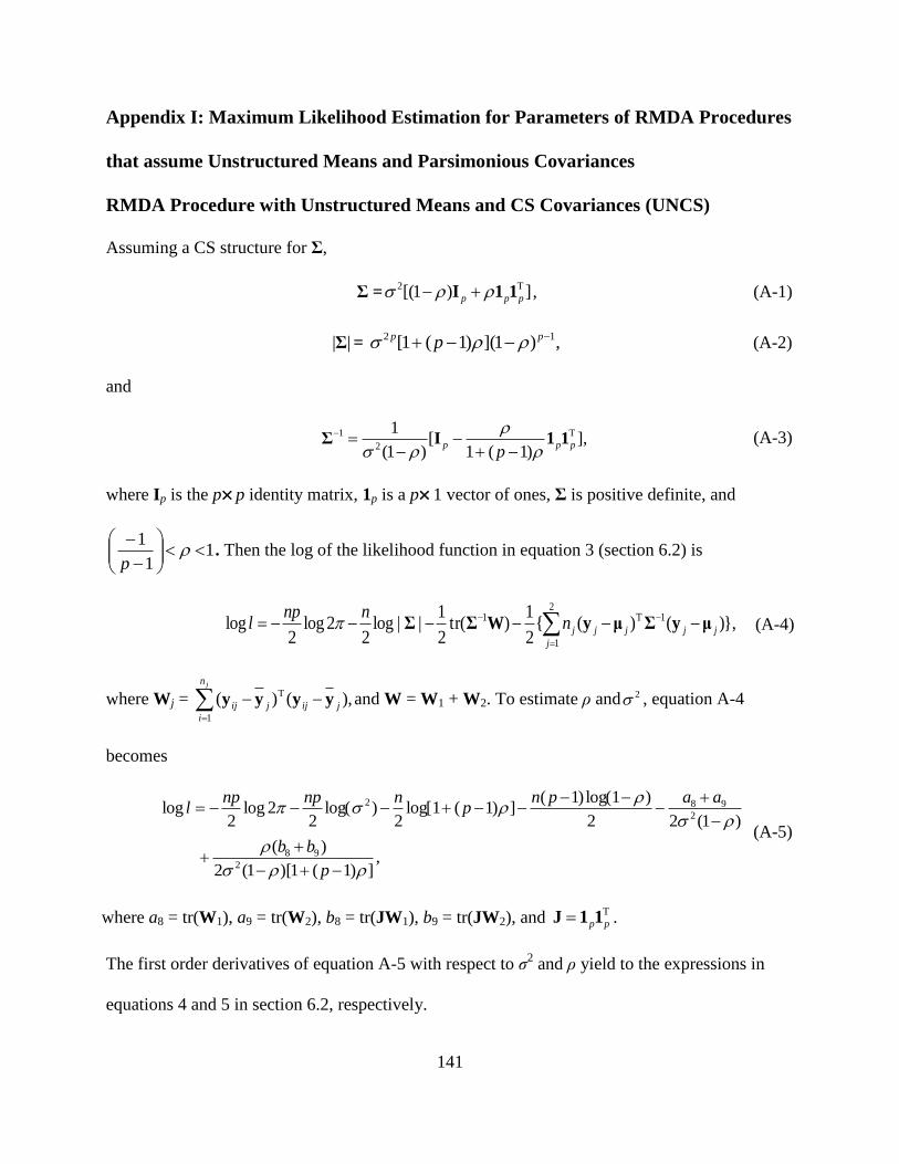
141

Appendix I: Maximum Likelihood Estimation for Parameters of RMDA Procedures

that assume Unstructured Means and Parsimonious Covariances

RMDA Procedure with Unstructured Means and CS Covariances (UNCS)

Assuming a CS structure for Σ,

Σ = ])1[( T2

ppp 11I , (A-1)

|Σ| = ,)1]()1(1[ 12 pp p (A-2)

and

],)1(1

[)1(

1 T

2

1

pppp

11IΣ

(A-3)

where Ip is the pp identity matrix, 1p is a p1 vector of ones, Σ is positive definite, and

11

1

p. Then the log of the likelihood function in equation 3 (section 6.2) is

},)()({2

1)(tr

2

1||log

22log

2log

2

1

1T1

j

jjjjjnnnp

l μyΣμyWΣΣ (A-4)

where Wj = ),()(1

T

jij

n

i

jij

j

yyyy

and W = W1 + W2. To estimate ρ and 2 , equation A-4

becomes

,])1(1)[1(2

)(

)1(22

)1log()1(])1(1log[

2)log(

22log

2log

2

98

2

982

p

bb

aapnp

nnpnpl

(A-5)

where a8 = tr(W1), a9 = tr(W2), b8 = tr(JW1), b9 = tr(JW2), and T

pp11J .

The first order derivatives of equation A-5 with respect to σ2 and ρ yield to the expressions in

equations 4 and 5 in section 6.2, respectively.

142

RMDA Procedure with Unstructured Means and AR-1 Covariances (UNAR)

For a AR-1 structured ,Σ

,)1(|| 122 pp Σ (A-6)

and

,)1( 122

01

p

ΣΣ (A-7)

where

1..........0

1.........0

................

0....10

001

0......01

2

2

2

0

Σ .

The joint log-likelihood function in equation 3 (see section 6.2) can be expressed as

)1(2

)(tr)1log(

2

)1(log

22log

2log

22

022

WΣpnnpnpl , (A-8)

where 2)(tr 10WΣ ,

11

11 ,)(tr

l mpl

lmpp

,

WWWW , )(Wtrα ,

W = W1 + W2, and Wij is the (i, j)th element of W. Equation A-8 simplifies to

)1(2

2)1log(

2

)1(log

22log

2log

22

222

pnnpnpl . (A-9)

The first order derivatives of equation A-9 with respect to σ2 and ρ yields the expressions in

equations 7 and 8 (section 6.2), respectively.

143

Appendix II: Supplementary Documentation

Description

This supplementary documentation contains SAS programming syntax (SAS Institute Inc., 2008)

to illustrate the implementation of repeated measures discriminant analysis procedures in non-

normal repeated measures data.

The documentation begins with syntax to read data from a .txt or .dat file into a file named

‘rsdata’ and a temporary SAS dataset called rmdaappendix. If the data are not in a .txt or .dat file,

then the syntax at the beginning of the program will change. Consult your SAS user’s manual or

contact the authors if you require assistance to prepare your dataset for use.

The documentation illustrates the syntax for data that contain six repeated measurements on a

HRQOL outcome. The data for the six repeated measurements are name y1, y2, y3, y4, y5,and

y6. The data also contain the numeric variable grp, which is used to discriminate between the

two study groups. The grp variable takes on values of 0 and 1. In this example, there are 45

observations (i.e., individuals) in group 1 and 25 observations in group 2. The group sizes must

be specified in the SAS program.

The components of the program that require user input are highlighted in boldface font.

The program will generate an error if there are missing data for any of the variables in the

dataset.

Reference

SAS Institute Inc. (2008). SAS/IML user's guide, version 9.2. Cary, NC: SAS Institute Inc.

144

SAS Syntax

**read in the data**;

filename rmdata 'Note to users: the dataset path and filename is inserted between the single

quotation marks';

data rmdappendix;

infile rmdata;

input grp y1 y2 y3 y4 y5 y6;

run;

**Use the IML procedure to read the dataset and its specifications**;

proc iml;

use rmdappendix;

read all var {y1 y2 y3 y4 y5 y6} into Y;

read all var {grp} into X;

x = design(x);

dv = ncol(y);

grpsz1 = 45; grpsz2 = 25;

ng = 2;

per = 0.2;

nj = {45 25};

ntot = 70;

bhat = inv(x`*x)*x`*y;

bhatw = bhat;

ss1 = J(dv,dv,0); ss2 = j(dv,dv,0);

145

ss1=((y#x[,1]-x[,1]*bhatw[1,])`*(y#x[,1]-x[,1]*bhatw[1,]));


sig = (ss1 +ss2)/(ntot-2);

/****************************************************************************

Module name: Trmn

Module Outputs:

bhat: Output matrix of least squares or trimmed means for each variable.

bhatw: Output matrix of group least squares or winsorized means for each variable

ytw: Output matrix of least squares of winsorized observations

***************************************************************************/

start trmn(trim, y, x, nj, bhat, bhatw, ytw, df) global(per,dv,ng);

ntot = sum(nj);

if trim=0 then do;

bhat=inv(x`*x)*x`*y;

bhatw=bhat;

ytw = y;

df=nj-1;

end;

if trim =1 then do;

bhat=J(ng,dv,0);

bhatw=bhat;

ytw = J(ntot,dv,0);

df=J(1,ng,0);

f=1;

146

m=0;

do j=1 to ng;

samp=nj[j];

l=m+samp;

g=int(per#samp);

df[j]=samp-2#g-1;

do k = 1 to ncol(y);

temp = y[f:l, k];

nv = temp;

temp[rank(nv),] = nv;

trimy = temp[g+1: samp-g,];

trimmn = sum(trimy)/(df[j]+1);

bhat[j,k] = trimmn;

mint = min(trimy);

maxt = max(trimy);

do p=1 to nrow(nv);

if nv[p]<=mint then nv[p] = mint;

if nv[p]>=maxt then nv[p] = maxt;

end;

ytw[f:l,k]=nv;

bhatw[j,k]=sum(nv)/samp;

end;

m = l;

147

f=f+nj[j];

end;

end;

finish;

/************************************************************************

Module Name: class_unstrmeanmod

Module Output: Output vector of discriminant function coefficients based on UNUN procedure

*************************************************************************/

start class_unstrmeanmod (y, x,bhat, bhatw,grpsz1,grpsz2,dv,dcoef1);

one = j(dv,1, 1);

n = nrow(y);

ybard=bhat[1,]-bhat[2,];



sig = (ss1 +ss2)/(n-2);

dcoef1= inv(sig)*(ybard)`;

finish class_unstrmeanmod;

/****************************************************************************

Module Name: ddacs_mod

Module Output: Output vector of discriminant function coefficients based on UNCS Procedure

***************************************************************************/

start ddacs_mod(y,x,bhat, bhatw, grpsz1, grpsz2, dv,dcoef2);

n = nrow(y);

148

b3 = J(dv,1,0);

ybar = y[+,]/n;

gp1 = y[1:grpsz1, ];

gp2 = y[grpsz1+1:n,];

jn = J(dv,dv,1);


w1=((y#x[,1]-x[,1]*bhatw[1,])`*(y#x[,1]-x[,1]*bhatw[1,]));


a8 = trace(w1); a9 = trace(w2); b8 = trace(jn*w1); b9 = trace(jn*w2);

/**** Estimating an initial estimate of rho****/

ybarn = repeat(ybar,n,1);

gp = y - ybarn;

gpass = gp[##,];

sq_gp = repeat(sqrt(gpass),n,1);

gpa = gp/sq_gp;

S = t(gpa)*(gpa);

rho1 = (s[+,+] - trace(s))/(dv*(dv-1));

sige = 0; iter = 0; converge = 0.0000001;

/***Evaluating the functions***/

do until(maxab< converge);

sig = ((1 + (dv-1)*rho1)*(a8+a9) - rho1*(b8+b9))/ (n*dv*(1-rho1)*(1 + (dv-1)*rho1));

absig = abs(sige - sig);

sige = sig;

149

/***Derivatives Function***/

k0 = n*(dv-1)*dv*sig;

pp = -((dv-2)*k0 - ((a8+a9)*(dv-1)**2) + (b8+b9)*(dv-1))/((dv-1)*k0);

qq =-(k0 - 2*(a8+a9)*(dv-1))/((dv-1)*k0);

rr = -(b8 + b9 - a8 - a9)/((dv-1)*k0);

aa = (1/3)*(3*qq-pp**2);

bb = (1/27)*(2*pp**3 - 9*pp*qq + 27*rr);

d = (bb**2)/4 + (aa**3)/27;

if d < 0 then s1 = 0;

else s1 = d**0.5;

s2 = (-bb/2 + s1)**(1/3);

ar = -bb/2 - s1;

if ar < 0 then do;

ar1 = -ar;

ar2 = ar1**(1/3);

s3 = -ar2;

end;

else do;

s3 = ar**(1/3);

end;

rho2 = s2 + s3 - pp/3;

iter = iter +1;

abr1 = abs(rho1 - rho2);

150

rho1 = rho2;

maxab = max(absig//abr1);

end;

sigm = (sig)*(( (1-rho2)*i(dv) + rho2*jn));

dcoef2 = inv(sigm)*(ybard)`;

finish ddacs_mod;

/**********************************************************************

Module Name: ddar

Module Output: Output vector of discriminant function coefficients based on UNAR

*********************************************************************/

start ddar (y, x, bhat, bhatw,grpsz1, grpsz2, dv,dcoef3);

n = nrow(y);

ybar = y[+,]/n;



gpbar1 = gp1[+,]/grpsz1;





w0 = w1 + w2;

a1 = trace(w0);

beta1 = trace(w0) - w0[1,1] - w0[dv,dv];

gama1 = 0;

151

do i = 1 to dv-1;

gama1 = gama1 + w0[i,i+1];

end;



gp = y - ybarn;

gpass = gp[##,];


gpa = gp/sq_gp;

S = t(gpa)*(gpa);

rho1 = (s[+,+] - trace(s))/(dv*(dv-1));


do until (maxab< converge);

sig = (beta1*rho1**2 - (2*gama1*rho1) + a1)/(n*dv*(1-rho1**2));

sige = sig;


pp = -(gama1) /(n*(dv-1)*sig);

qq =-(n*(dv-1)*sig - (a1+beta1))/(n*(dv-1)*sig);

rr = -(gama1)/(n*(dv-1)*sig);

aa = (1/3)*(3*qq-pp**2);

bb = (1/27)*(2*pp**3 - 9*pp*qq + 27*rr);

d = (bb**2)/4 + (aa**3)/27;

if d < 0 then s1 = 0;

152

else s1 = d**0.5;

s2 = (-bb/2 + s1)**(1/3);

ar = -bb/2 - s1;

if ar < 0 then do;

ar1 = -ar;

ar2 = ar1**(1/3);

s3 = -ar2;

end;

else do;

s3 = ar**(1/3);

end;

rho2 = s2 + s3 - pp/3;

iter = iter +1;


rho1 = rho2;


end;

v = J(dv,dv,0);

do i = 1 to dv;

do j = 1 to dv;

v[i,j] = sig*rho2**(abs(i-j));

end; end;

dcoef3 = inv(v)*(ybard)`;

153

finish ddar;

/****************************************************************************

Module Name: royddacs_mod

Module Output: Output vector of discriminant function coefficients based on STCS Procedure

*****************************************************************************/

start royddacs_mod(y,x, bhat, bhatw, grpsz1, grpsz2, dv,dcoef4);

n = nrow(y);

one = j(dv, 1, 1);

b3 = J(dv,1,0);

ybar = y[+,]/n;





mu1 = bhat[1,]*one/dv;


mn1 = mu1* one;

mn2 = mu2 * one;

w1 = J(dv,dv,0);

w2 = J(dv,dv,0);

jn = J(dv,dv,1);



154


a8 = trace(w1); a9 = trace(w2); b8 = trace(jn*w1); b9 = trace(jn*w2);



gp = y - ybarn;

gpass = gp[##,];


gpa = gp/sq_gp;

s = t(gpa)*(gpa);

rho1 = (s[+,+] - trace(s))/(dv*(dv-1));


/***Evaluating the functions***/


sig = ((1 + (dv-1)*rho1)*(a8+a9) - rho1*(b8+b9))/ (n*dv*(1-rho1)*(1 + (dv-1)*rho1));


sige = sig;

/***Derivatives Function***/

k0 = n*(dv-1)*dv*sig;

pp = -((dv-2)*k0 - ((a8+a9)*(dv-1)**2) + (b8+b9)*(dv-1))/((dv-1)*k0);

qq =-(k0 - 2*(a8+a9)*(dv-1))/((dv-1)*k0);

rr = -(b8 + b9 - a8 - a9)/((dv-1)*k0);

aa = (1/3)*(3*qq-pp**2);

bb = (1/27)*(2*pp**3 - 9*pp*qq + 27*rr);

155

d = (bb**2)/4 + (aa**3)/27;

if d < 0 then s1 = 0;

else s1 = d**0.5;

s2 = (-bb/2 + s1)**(1/3);

ar = -bb/2 - s1;

if ar < 0 then do;

ar1 = -ar;

ar2 = ar1**(1/3);

s3 = -ar2;

end;

else do;

s3 = ar**(1/3);

end;

rho2 = s2 + s3 - pp/3;

iter = iter +1;


rho1 = rho2;


end;

sigm = (sig)*(( (1-rho2)*i(dv) + rho2*jn));

dcoef4 = inv(sigm)*(mn1 - mn2);

finish royddacs_mod;

156

/*****************************************************************************

Module Name: royddar_mod

Module Output: Output vector of discriminant function coefficients based on STAR Procedure

*****************************************************************************/

start royddar (y,x, bhat, bhatw, grpsz1, grpsz2, dv,dcoef5);

one = J(dv, 1, 1);

n = nrow(y);

ybar = y[+,]/n;







mn1 = mu1* one;

mn2 = mu2 * one;




w3 = bhatw[1,]`*bhatw[1,];

w4 = bhatw[2,]`*bhatw[2,];

w5 = one*bhatw[1,] + bhatw[1,]`*one`;

w6 = one*bhatw[2,] + bhatw[2,]`*one`;

157

w0 = w1 + w2+ grpsz1*w3 + grpsz2*w4;

a1 = trace(w0);

a2 = trace(w5);

a3 = trace(w6);




gama1 = 0;

gama2 = 0;

gama3 = 0;

do i = 1 to dv-1;

gama1 = gama1 + w0[i,i+1];

gama2 = gama2 + w5[i, i+1];

gama3 = gama3 + w6[i, i+1];

end;

cc = grpsz1*(mu1**2) + grpsz2*(mu2**2);



gp = y - ybarn;

gpass = gp[##,];


gpa = gp/sq_gp;

s = t(gpa)*(gpa);

158

rho1 = (s[+,+] - trace(s))/(dv*(dv-1));



sig = ((beta1 - grpsz1*mu1*beta2 - grpsz2*mu2*beta3 + cc*(dv - 2))*(rho1**2) - 2*(gama1 -

grpsz1*mu1*gama2 - grpsz2*mu2*gama3 + cc*(dv-1))*(rho1) +

(a1 - grpsz1*mu1*a2 - grpsz2*mu2*a3 + cc*dv))/(n*dv*(1-rho1**2));

sige = sig;


pp = -(gama1-grpsz1*mu1*gama2 - grpsz2*mu2*gama3 + cc*(dv-1)) /(n*(dv-1)*sig);

qq =-(n*(dv-1)*sig - (a1+beta1) + grpsz1*mu1*(a2+ beta2) + grpsz2*mu2*(a3 + beta3) -

cc*(2*dv-2))/(n*(dv-1)*sig);

rr = -(gama1- grpsz1*mu1*gama2 - grpsz2*mu2*gama3 + cc*(dv-1) )/(n*(dv-1)*sig);

aa = (1/3)*(3*qq-pp**2);

bb = (1/27)*(2*pp**3 - 9*pp*qq + 27*rr);

d = (bb**2)/4 + (aa**3)/27;

if d < 0 then s1 = 0;

else s1 = d**0.5;

s2 = (-bb/2 + s1)**(1/3);

ar = -bb/2 - s1;

if ar < 0 then do;

ar1 = -ar;

ar2 = ar1**(1/3);

s3 = -ar2;

159

end;

else do;

s3 = ar**(1/3);

end;

rho2 = s2 + s3 - pp/3;

iter = iter +1;


rho1 = rho2;


end;

v = J(dv,dv,0);

do i = 1 to dv;

do j = 1 to dv;

v[i,j] = sig*rho2**(abs(i-j));

end; end;

dcoef5 = inv(v)*(mn1 - mn2);

finish royddar;

****Compute Discriminant Function Coefficients based on ML Estimation;

trim = 0;

cal trmn(trim, y, x, nj, bhat, bhatw, ytw, df);

call class_unstrmeanmod (y, x,bhat, bhatw,grpsz1,grpsz2,dv,dcoef1);

call ddacs_mod(y,x,bhat, bhatw, grpsz1, grpsz2, dv,dcoef2);

call ddar (y,x, bhat, bhatw, grpsz1, grpsz2,dv,dcoef3);

160

call royddacs_mod(y, x, bhat, bhatw, grpsz1, grpsz2,dv, dcoef4);

call royddar (y,x, bhat, bhatw, grpsz1, grpsz2,dv,dcoef5);

****Compute Discriminant Function Coefficients based on CT Estimation;

trim = 1;

call trmn(trim, y, x, nj, bhat, bhatw, ytw, df);

call class_unstrmeanmod (ytw, x,bhat, bhatw,grpsz1,grpsz2,dv,tdcoef1);

call ddacs_mod(ytw,x,bhat, bhatw, grpsz1, grpsz2, dv,tdcoef3);

call ddar (ytw,x, bhat, bhatw, grpsz1, grpsz2,dv,tdcoef3);

call royddacs_mod(ytw, x, bhat, bhatw, grpsz1, grpsz2,dv, tdcoef4);

call royddar (ytw,x, bhat, bhatw, grpsz1, grpsz2,dv,tdcoef5);

Print 'Vector of DFCs for UNUN Procedure based on ML Estimators;' dcoef1[format =8.2];

Print 'Vector of DFCs for UNUN Procedure based on CT Estimators;' tdcoef1[format =8.2];

Print 'Vector of DFCs for UNCS Procedure based on ML Estimators;' dcoef2[format =8.2];

Print 'Vector of DFCs for UNCS Procedure based on CT Estimators;' tdcoef2[format =8.2];

Print 'Vector of DFCs for UNAR Procedure based on ML Estimators;' dcoef3[format =8.2];

Print 'Vector of DFCs for UNAR Procedure based on CT Estimators;' tdcoef3[format =8.2];

Print 'Vector of DFCs for STCS Procedure based on ML Estimators;' dcoef4[format =8.2];

Print 'Vector of DFCs for STCS Procedure based on CT Estimators;' tdcoef4[format =8.2];

Print 'Vector of DFCs for STAR Procedure based on ML Estimators;' dcoef5[format =8.2];

Print 'Vector of DFCs for STAR Procedure based on CT Estimators;' tdcoef5[format =8.2];

quit;

161

Section III. Variable Importance Measures for Multivariate

Repeated Measures Data

162

Chapter 7. Variable Importance Measures

Abbreviations




DRC = Discriminant ratio coefficient

FTR = F-to-remove statistic


MANOVA = Multivariate analysis of variance


SDFC = Standardized discriminant function coefficient

SC = Structure coefficient

TDRC = Total discriminant ratio coefficient

163

7.1 Introduction

In clinical investigations involving the comparison of two groups (i.e., treatment and

control), data are often collected on a battery of outcomes. It is often desirable to test for

differences between groups and to identify the variables that predict differences between groups.

Global tests of group differences can be obtained using multivariate procedures, such as

multivariate analysis of variance (MANOVA)1-2

. Following a significant overall test of

differences between groups, researchers may be interested in identifying the domains that

discriminate between groups. The conventional approach is to conduct multiple tests of

significance for evaluating group differences on the outcomes using an appropriate multiple

testing procedure to control the overall probability of type I error3-4

. The variables that are

statistically significant are considered to be the most important variables that discriminate

between groups.

Relative importance analysis is another approach for identifying the most important

variables that discriminate between groups. The concept of variable importance, which has been

historically subject to diverse interpretations in the statistics literature and in many disciplines5-7

,

was first developed within the regression model framework for quantifying the relative

importance of explanatory variables in predicting an outcome. In recent years, the concept of

variable importance has been extended to describe the relative importance of outcome variables

in multivariate group designs using descriptive discriminant analysis (DDA) models.

In DDA, one or more linear combinations of the variables that maximize group separation

are identified and the discriminant function coefficients (DFCs) from DDA are used to rank the

variables according to their contribution to group separation8. Several measures of relative

importance based on DFCs have been proposed including standardized discriminant function

164

coefficients (SDFCs)9-10

, structure coefficients (SCs), discriminant ratio coefficients (DRCs)11

,

total discriminant ratio coefficients (TDRCs)12

, and F-to-remove (FTR) statistics9,13

. Relative

importance measures can be used to rank order outcome variables based on their ability to

discriminate between groups. These measures are now being adopted for identifying variables

that discriminate between groups in several disciplines14,15

. They are also useful for testing

hypothesis about differences in the DFCs and/or ranks of variables16

.

In this chapter, measures of relative importance derived from the DFCs of DDA are

described. A number of issues that arise in the assessment of relative importance of variables are

also discussed.

7.2 Description of Measures of Relative Importance for Multivariate Group

Designs

In two-group multivariate designs, Huberty and Wisenbaker9 defined variable importance

as the relative contribution of a variable to group discrimination. More specifically, they defined

the relative importance of a variable as (a) its contribution to a latent variable, (b) its contribution

to a linear discriminant function, and (c) its contribution to a grouping variable effect. These

measures, which are functions of the DFCs, are used to rank the variables based on their

contribution to group separation.

Let yij be the p 1 vector of observed measurements for the ith study participant (i = 1,...,

nj) in the jth group (j = 1, 2, N = n1 + n2). Assume that yij ~ Np(μj, Σj), where μj and Σj are the

population mean and covariance for the jth group and are estimated by jμ and jΣ , respectively.

For the linear discriminant analysis (DA) procedure, the DFC vector is estimated by

165

)ˆˆ(ˆˆ21

1μμΣa , (1)

where

.2

ˆ)1(ˆ)1(ˆ

21

2211

nn

nn ΣΣΣ (2)

The number of uncorrelated discriminant functions that separates g groups is equal to g – 1.

The SDFC is one commonly adopted measure of relative importance. It is a unitless

measure that range from -1 to 1. The SDFC quantifies the relative importance of a variable by

taking into account the presence of other variables in the study. While there have been arguments

in favour of using SDFCs to measure relative importance17,18

, they are known to be sensitive to

correlation among the variables18

.

The SDFC for the kth variable is,

,*

kkk saa (3)

where ak and sk are the DFC and standard deviation on the kth variable, respectively. SDFCs can

be positive or negative, and the absolute magnitude determines relative importance.

The SC is the correlation between a DFC and the individual variable. SCs are particularly

useful for assessing variable importance because they provide direct information about the

relationship between a discriminant function and an outcome variable. However, Rencher and

Scott19

have argued against using SCs because they do not take into account the presence of

other variables.

DRC9,10

measures the relative importance of a variable as a proportion of the group

differences explained by this variable. The DRC is given by

,*

kkk faq (4)

where *

ka and fk are the SDFC and SC for the kth variable, respectively. DRC values typical range

166

between 0 and 1, although negative values indicate potential collinearity among the variables or

the presence of suppressor variables. Suppression occurs when a variable makes little or no

direct contribution to group separation on its own but contributes to group separation indirectly

through another variable.

Thomas and Zumbo13

proposed the TDRC to measure relative importance. The TDRC

for the kth variable is

)(

||

T

T

aaS

S kkkk

at , (5)

where STkk is the (k,k)th element of ST, ST = T/ (N – 1), T = H + E,

2

1

T

1

))((j

jij

n

i

jij

j

yyyyE , (6)

is the error sum of squares and cross product matrix,

2

1

T))((j

jjjn yyyyH , (7)

is the hypothesis sum of squares and cross product matrix, and T is the transpose operator.

TDRCs can take values within the interval [0, ∞), with a larger value indicating greater relative

importance.

The FTR9,13

for the kth variable is

2

)(321

2

)(2

)()/()(

)/(

kkk

kkk

ksakzz

sakF

, (8)

where ),2(2 pNk ,/ 21

2

3 nnNk ak is the DFC for the kth variable, 21 and zz are the group

means for the discriminant function score corresponding to a, and s(kk) is the positive square root

167

Table 7-1. Measures of Relative Importance for Multivariate Group Designs

Measure Description Advantages Limitations

SDFC 1. A product of the estimated

DFC and the standard

deviation on each variable.

2. Ranks variables based on

the absolute values of the

SDFC

1. It is a unitless measure

2. Evaluates importance

while accounting for the

presence of other study

variables

3. Available in existing

software

1. It is sensitive to

correlation among

the variables

2. May not be

appropriate when

there are suppressor

variables in the

study

SC 1. A measure of correlation

between each variable and

the discriminant function

score.

2. SC values range between 0

and 1.

1. Evaluates the

importance of a variable

as its contribution to the

discriminant function.

2. Available in existing

software

1. A univariate

measure of

correlation that does

not account for the

presence of other

study variables

DRC 1. A product of the SDFC

and the structure

coefficient. It quantifies

the relative importance of

a variable as the

proportion of the group

differences explained by

1. It satisfies all axioms

about variable

importance.

2. Recommended as the

most reliable measure of

relative importance.

3. Robust to several data


correlation among

the variables.

2. Not to easy to

compute in existing

software

168

the variable.

2. DRC values range

between 0 and 1.

characteristics

TDRC 1. A variant of the SDFC that

uses the total error sum of

squares and cross product

matrix to standardize the

DFCs.

2. TDRC takes values in the

interval [0, ∞).

1. TDRC has been

recommended as a

measure for identifying

suppressor variables

when used in conjunction

with the DRC.


the magnitude of

correlation among

the variables.

FTR

statistic

1. A variant of the step-wise

multivariate analysis of

variance (MANOVA)

measure.

2. The FTR statistic takes

values in the interval [0,

∞)

1. The FTR statistic

quantifies the importance

of a variable as its

contribution to a grouping

effect.

2. Evaluates the unique

contribution of a variable

to a grouping effect

1. The FTR statistic

does not account for

the presence of

other study

variables.

of the kth diagonal element of the inverse of E, which is defined in equation 6. The FTR can take

values within the interval [0, ∞), with a larger value indicating greater relative importance.

The strengths and limitations of these measures of relative importance are summarized in

169

Table 7-1.

7.3 Statistical Inference about Variable Importance

While measures of relative importance can be used in exploratory analyses to identify the

most important variables, there are limited investigations about whether the size of the DFC for a

variable is large enough to suggest that the variable is important. The conventional rule of thumb

is one approach often used by applied researchers to evaluate if the magnitude of the relative

importance measure is large enough to determine if a variable is important. This includes setting

cut off points, to determine what size is important20,21

. For example, variables with DRC values

above 1/2p can be considered important while variables with negative DRC values are suggested

to be suppressor variables with no direct contribution to group separation. However, given that

sample estimates of DFCs of variable rankings ignore the sample error in that data, such rules of

thumb are sensitive to sample size and the number of variables in the study.

Assessing statistical significance of a variable’s DFC provides an alternative approach for

evaluating the size of a variable’s DFC in relation to variable importance. A number of

parametric and non-parametric tests of significance of DFCs have been described in the

literature..

Statistical significance based on the theoretical distribution of the DFCs is another valid

approach proposed for testing if a variable’s rank is significantly different from zero. Parametric

tests based on asymptotic theory have been developed to test for statistical significance of

DFCs16, 22

. For example, Rao16

proposed an F-test to evaluate statistical significance of a

variable’s contribution to group separation. This test is given as

170

),1(~)(

))((2

)(3

2

)(

2

* pnFDpnk

DDpnF

k

k

k

, (9)

where )()(21

1T

21

2yySyy D , and 2

)(kD is the value of D2 when the kth variable is omitted

from the analysis. For this test, the null hypothesis is that the DFC for the kth variable is equal to

zero (i.e., H0: ak = 0; H1: ak ≠ 0). A statistically significant ak suggests that the kth variable’s

contribution to group separation is statistically significant.

More recently, Bodnar and Okhirin23

derived a more general statistic for testing statistical

significance of a variable’s DFCs or testing differences between the DFCs of two variables.

Define T as

1

21

T

21

1T~

)(ˆ)(1ˆ

ˆ1

pn

L

tpnTμμRμμLΣL

aL, (10)

where LΣLΣLLΣΣR11T11 ˆ/ˆˆˆˆ T

, and L is a contrast vector corresponding to the variable

DFCs being tested. Similarly, these parametric tests can be used to derive confidence intervals

for the DFC for each variable. However, these parametric tests are sensitive to departures from

the underlying assumptions of DDA and may not perform well when the sample size is small.

Re-sampling based statistical methods10, 24

that repeatedly sample from the original data,

are alternative methods for testing hypothesis about statistical significance of DFCs or for testing

differences between the ranks of two variables. Dalgleish24

tested for statistical significance of

structure coefficients by constructing approximate confidence intervals using a Jacknife

technique and concluded that bootstrap confidence intervals provide a more reliable way to

evaluate statistical significance of a variable’s importance. For the FTR statistic, Huberty and

Wisenbaker10

proposed two statistical tests based on bootstrap methods for testing if a variable is

statistically important and whether two variables are statistically equal in importance. Given that

171

resampling-based methods do not assume a parametric distribution, they are particularly useful

for assessing statistical significance of a variable’s importance when the data distribution is not

known. This methodology has been used with other variable importance measures (such as

relative weights and Pratt’s index) in the regression literature for testing hypotheses and

constructing confidence intervals25, 26

.

7.4 Discussion

While previous research has shown that there is a lack of agreement about the “best”

measure of relative importance, these measures may not always result in consistent rankings of a

set of variables27-28

. Dissimilarities in rankings may arise, in part, because of data characteristics

and deviations from the assumptions of multivariate normality and homogeneity (i.e., equality)

of group covariance matrices. When the assumptions of the DDA model are satisfied, these

measures result in correct rank ordering of the variables because DDA has greater statistical

power to discriminate between groups. However, under assumption violations, these measures

may result in incorrect rank ordering of the variables19

.

Moreover, data characteristics such as collinearity and suppression effects can also influence

the consistency of variable rankings for these measures. For example, when the DRC is used to

rank order the variables according to their contribution to group separation, an exclusion of

variables with large negative DRC values (due to suppression or collinearity) from the analysis

has been recommended12

. In contrast, other variable importance measures, which are not

sensitive to suppression effect, may rank this variable as important. Hence, DRCs may result in a

different rank ordering of the variables than other measures of relative importance when

suppressor variables are excluded from the analysis.

Although variable importance measures have been developed mainly for descriptive

172

purposes, they are also useful for inferential analyses. For example,tests of the significance of

sample variable ranks may be conducted in order to generalize conclusions about variable

importance to the population. Hypotheses about whether there is a statistically significant change

in a variable importance over two measurement occasions may also be tested using measures of

relative importance. However, although a number of approaches for evaluating statistical

significance of variable importance ranking have been described in section 7.3, the statistical

power and Type I error rates of these tests have not been investigated. Moreover, the measures of

relative importance described here have only been applied to rank order a set of correlated

variables in multivariate data collected at a single time point. There is limited investigation about

their application in evaluating the relative importance of variables in multivariate repeated

measures data. Such data often arise in longitudinal studies in which multiple outcomes are

measured at two or more measurement occasions. In these studies, researchers seek to

understand the most important HRQOL dimensions on which the differences between groups are

maximized. Measures of relative importance have potential applications in identifying the most

importance variables on which group

The measures of importance described in this chapter assume complete data on all

variables, with casewise deletion of study participants with incomplete data. However, casewise

deletion can result in biased estimates of relative importance when the mechanism of

missingness is not random29

. While an imputation method29

could be adopted when there are

missing values, the statistical theory underlying DA procedures based on imputation methods are

yet to be developed.

There are additional considerations when conducting a relative importance analysis. The

conclusion that one variable is more important than another can only be applied to the set of

173

variables under investigation. Hence, changing the variable set included in the analysis may

result in different conclusions about relative importance. As well, relative importance may be

associated with covariates such as age and sex. Stratified analyses might be conducted to assess

the influence of covariates on the results. Alternatively, covariates can be incorporated into the

mean of the DA model by conditioning on the covariates and by adopting a multivariate analysis

of covariance model30

.

Relative importance measures have a number of potential uses in exploratory and inferential

research. In exploratory research, they can be used to identify a small set of domains on which to

focus in future studies. The measures could be used to assign weights to the domains when using

a multiple testing procedure to control the overall probability of a Type I error; procedures in

which the weights are assigned a priori have been shown to result in substantially improved

power to detect group differences on the most important variables31-32

.

More recently, DA procedures that assume parsimonious means and covariance structures

have been developed for predicting group memberships in repeated measures data33-35

. Although

these procedures are advantageous for classification in studies with small sample size, there are

limited investigations of their application for describing the relative importance of

variables/measurement occasions in repeated measures data. Given that the DFCs of DDA

procedures can be used to quantify the relative importance of variable in multivariate group

designs, DFCs from the repeated measures discriminant analysis (RMDA) procedures can also

be used to describe the relative contribution of variables and measurement occasions in

multivariate repeated measures data. Measures of relative importance based on these RMDA

procedures could be useful in longitudinal health-related quality of life (HRQOL) studies in

which researchers seek to understand the most important HRQOL domains on which the

174

differences between groups are maximized36

. The next chapter proposes new methods for

evaluating the relative importance of variables in multivariate repeated measures data with a

numeric example from a longitudinal HRQOL study.

175

References

1. Fairclough, D. L. (2002). Design and Analysis of Quality of Life Studies in Clinical Trials.

New York: Chapman & Hall.

2. Sheehan-Holt, J. K. (1998). MANOVA simultaneous test procedures: The power and

robustness of restricted multivariate contrasts. Journal of Educational and Psychological

Measurement, 58, 861 – 881.

3. Timm, N. H. (2006). Applied Multivariate Analysis. New York: Springer-Verlag.

4. Lix, L. M & Sajobi, T. T. (2010). Testing multiple outcomes in repeated measures data.


5. Tabachnik, B. G., & Fidell, L. S. (2001). Using multivariate statistics, 4th

edition. Boston:

Allyn & Bacon.

6. Healy, M. J. R. (1990). Measuring importance. Statistics in Medicine, 9, 633 – 637.

7. Johnson, J. W. (2000). A heuristic method for estimating the relative weight of predictor

variables in multiple regression. Multivariate Behavioral Research, 35, 1 – 19.

8. Huberty, C. J., & Olejnik, S. (2006). Applied MANOVA and Discriminant Analysis. New

York: Wiley.

9. Huberty, C. J. (1984). Issues in the use and interpretation of discriminant analysis.

Psychological Bulletin, 95, 156 – 171.

10. Huberty, C. J., & Wisenbaker, J. M. (1992). Variable importance in multivariate

group comparisons. Journal of Educational Statistics, 17, 75 – 91.



176

12. Thomas, D. R. (1997). A note Huberty and Wisenbaker’s “Views of variable importance”.

Journal of Educational and Behavioural Statistics, 22, 309 – 322.




14. Sajobi, T. T., Lix, L.M., Clara, I., et al. (2012). Measures of relative importance for health-


15. Lievens, F., Van Hoye, G., & Schreurs, B. (2005). Examining the relationship between

employer knowledge dimensions and organizational attractiveness: An application in a

military context. Journal of Occupational and Organizational Psychology, 78, 553 – 572.

16. Rao, C. R. (1970). Inference on discriminant coefficients. In Essays in probability and

statistics, Bose et al. (Eds), 587 – 602. North Carolina: University of North Carolina.

17. Rencher, A. C. (1995). Methods of Multivariate Analysis. New York: Wiley.

18. Rencher, A. C., & Scott, D. T. (1990). Assessing the contribution of individual variables

following rejection of a multivariate hypothesis. Communications in Statistics – Simulation

and Computation, 19, 535 – 553.

19. Rencher, A. C. (1992). Interpretation of canonical discriminant functions, canonical variates,

and principal components. The American Statistician, 46, 217 – 225.

20. Ochieng, C. O., & Zumbo, B. D. (2001). Examination of a variable ordering index in linear

regression models: An assessment of the relative Pratt index in Likert data. Paper presented

at the Bob Conry Conference on Measurement Evaluation and Research and Methodology,

Vancouver, Canada.

177

21. Tabachnick, B. G., & Fidell, L. S. (1989). Using Multivariate Statistics (2nd Edition). New

York: Harper & Row.

22. Radcliffe, J. (1968). A note on the construction of confidence intervals for the coefficients of

a second canonical variable. Proceedings of the Cambridge Philosophical Society, 64, 471 –

475.

23. Bodnar, T., & Okhirin, Y. (2011). On the product of inverse Wishart and normal distributions

with applications to discriminant analysis and portfolio theory. Scandinavian Journal of

Statistics, 38, 311 – 331.

24. Dalgleish, L. I. (1994). Discriminant analysis: Statistical inference using the jackknife and

bootstrap procedures. Psychological Bulletin, 116, 498 – 508.

25. Tonidandel, S., Lebreton, J. M., & Johnson, J. W. (2009). Determining statistical significance

of relative weights. Psychological Methods, 14, 387 – 399.

26. Thomas, D. R., Zhu, P., & Decady, Y. J. (2007). Point estimates and confidence intervals for

variable importance in multiple linear regression. Journal of Educational and Behavioural


27. Finch, W. H., & Laking, T. (2008). Evaluation of the use of standardized weights for

interpreting results from a descriptive discriminant analysis. Multiple Linear Regression

Viewpoints, 34, 19 – 34.

28. Huberty, C. J. (1975). The stability of three indices of relative variable contribution in

discriminant analysis. Journal of Experimental Education, 44, 59 – 64.

29. Little, R. J. A., & Rubin, D. B. (2002). Statistical Analysis with Missing Data (2nd Edition).

New Jersey: Wiley.

30. Kim, K., & Timm, N. (2007). Univariate and Multivariate General Linear Models: Theory

178

and Applications with SAS (2nd Edition). New York: Chapman & Hall/CRC.

31. Benjamini, Y., & Hochberg, Y. (1997). Multiple hypothesis testing with weights.

Scandinavian Journal of Statistics, 24, 407 – 418.

32. Maurer, W., Hothorn, L. A., & Lechmacher, W. (1995). Multiple comparisons in drug

clinical trials and preclinical assays: A priori ordered hypotheses. In Vollman, J., (Ed),

Biometrie in der chemische-pharmazeutichen Industrie (Vol. 6). Stuttgart: Fischer Verlag.

33. Lix, L. M. & Sajobi, T. T. (2010) Discriminant analysis for repeated measures data: a review.

Frontiers in Quantitative Psychology and Measurement, 1, 1 – 9.






36. Feighner, J. P., & Sverdlov, L. (2002). The use of discriminant analysis to separate a study

population by treatment subgroups in a clinical trial with a new pentapeptide antidepressant.

Journal of Applied Research, 2, 17 – 18.

179

Chapter 8. Evaluation of Variable Importance in Multivariate Repeated Measures

Data

Tolulope T. Sajobi1

Lisa M. Lix1,2

Longhai Li2

William H. Laverty2

1School of Public Health, University of Saskatchewan, Saskatoon, CANADA

2Department of Mathematics & Statistics, University of Saskatchewan, Saskatoon, CANADA

180

Abbreviations

AR-1 = First-order autoregressive structure

CS = Compound symmetric structure




IBDQ = Inflammatory Bowel Disease Questionnaire




UN = Unstructured

UNAR = DA based on unstructured means and covariances with a AR-1 structure

UNCS = DA based on unstructured means and covariances with a CS structure


181

Abstract

Repeated measures discriminant analysis (RMDA) procedures that assume parsimonious

covariance structures have been recently developed for predicting group membership in

multivariate repeated measures data, in which two or more outcome variables are repeatedly

measured at more than two measurement occasions. However, there is less emphasis on the use

of the discriminant function coefficients of these procedures for evaluating the relative

importance of variables in multivariate repeated measures data. This study compares

standardized discriminant function coefficients (SDFCs) of two RMDA procedures based on

their ability to correctly rank order variables according to their ability to discriminate between

groups. These include the stagewise RMDA procedure and an RMDA procedure that assume

Kronecker product covariance structures. Monte Carlo techniques were used to evaluate the

SDFCs of these procedures for different conditions of number of variables, total sample size,

mean configuration, and correlation structure. Percentages of any-variable and average per-

variable correct rankings were evaluated. Overall, SDFC based on the average of with-variable

DFCs for RMDA procedure that assume Kronecker product covariance structure resulted in the

highest percentages of correct rankings and largest concordance values. Moreover, the SDFCs

for these RMDA procedures are sensitive to the magnitude of separation between group means,

and the magnitude of variable correlation. Variable importance measures are an important tool

identifying the most importance outcome that discriminate between groups in multivariate


Key words: relative importance; multivariate repeated measures data; discriminant analysis;

Kronecker product; covariance structure

182

8.1 Introduction

Multivariate repeated measures data in which q ≥ 2 outcome variables are measured at

p ≥ 2 measurement occasions are common in medical and social science research studies that

compares groups of individuals for efficacy of treatment or interventions. For example, a recent

review of research studies on psychotherapy for the treatment of youth mental health disorders

suggests that this literature abounds with studies in which participants exposed to child-, parent-,

family-, or teacher-focused interventions were compared with participants randomized to a

placebo condition, standard case management protocol, or alternate treatment, on multiple

measures of patient symptoms, behaviours, level of functioning, and psychosocial responses1.

Longitudinal health-related quality of life data are another example of multivariate repeated

measures data. They consist of individuals’ ratings on multiple inter-related domains, such as

mental health, physical function, and social function, which are collected at multiple occasions

following disease diagnosis or treatment2-3

.

There are several reasons why a researcher might test for group differences on multiple

outcome variables that are measured on multiple occasions. Researchers may be interested

modeling the joint evolution of outcome variables or in understanding how that evolution differs

for different groups of study participants. In clinical trials, for example, differences between

treatment and control groups or severely ill versus less severely ill patients may be examined.

There may be limited research knowledge about which outcome(s) will be the responsive to

treatment.

While multivariate data are usually characterized by between variable correlations,

multivariate repeated measures data contain two sources of correlation: (a) within-variable

correlation, which arises because the repeated measurements for each outcome variable are

183

correlated and (b) between-variable correlation, which arises because the responses on the

outcome variables at each measurement occasion are correlated. Statistical procedures that

accounts for both correlation sources include procedures for testing omnibus hypotheses of no

group differences4-6

such as repeated measures analysis of variance (RMANOVA) and analysis

of covariance (ANCOVA). Post-hoc multiple testing procedures7 have also been proposed for

identifying the outcomes on which group differences exist in multivariate repeated measures

studies. Moreover, classification models, such as repeated measures discriminant analysis

(RMDA) procedures that assume structured covariances, have been proposed for predicting

disease status in multivariate repeated measures data8-11

. One model is based on a stage-wise

discriminant analysis procedure, in which within-variable growth trends are summarized using

regression functions (Stage 1) and a DA classification rule is developed based on the subject–

specific predicted scores from the regression functions (Stage 2). More recently, RMDA models

that assume parsimonious means and/or covariances have been developed for discrimination in

multivariate repeated measures data12-13

. These procedures, which assume Kronecker product

structure, are particularly advantageous when the sample size is small relative to data dimension.

However, these procedures have focused on prediction and not description of group separation.

Variable importance analysis based on discriminant function coefficients provides an

alternative approach for identifying the most important outcomes that are responsive to treatment

in multivariate repeated measures data. These measures have been developed to rank a set of

variables according to their ability to discriminate between groups in multivariate data14-15

, but

there have been few studies in which these methods have been extended to multivariate repeated

measures data. Methods that have been proposed to evaluate the variable importance in

multivariate repeated measures studies include assigning ranks to a set of variables using

184

discriminant function coefficients (DFCs) from descriptive discriminant analysis (DDA) to the

baseline data16-17

, or ranking variables based on measures of relative importance derived from

applying DDA to subject-specific longitudinal change scores18-19

. These methods do not account

for within-variable and between-variable correlation and may be inefficient when the sample size

is small relative to the number of variables.

Given this background, the purpose of this study is to develop variable importance

measures based on the DFCs of RMDA procedures that assume Kronecker product covariance

structures for evaluating variable importance in multivariate repeated measures data. Their

performance under a variety of data analytic conditions is examined using Monte Carlo

techniques and data from the longitudinal cohort study are used to demonstrate their

implementation.

8.2 Methods

Let yij be the pq 1 vector of observed measurements corresponding to p repeated

measurements on each of the q outcome variables for the ith study participant in the jth group (i

= 1, ..., nj; j = 1, 2; n = n1 + n2).The vectors are structured such that the repeated measurements

are nested within each variable. Assume that yij ~ Npq(μj, Ωj), where μj and Ωj= Ω are the

population mean and covariance for the jth group and are estimated by jμ and ,Ω respectively.

Here, we describe three methods for evaluating the relative importance of variables in

multivariate repeated measures data.

Method 1 is a stagewise procedure, in which DFCs are estimated separately for each

outcome variable using RMDA procedure and then used to estimate subject-specific discriminant

function score for each variable (stage 1). Standardized discriminant function coefficients

185

(SDFC), which are estimated from the discriminant function score data, are then used to rank

order the variables (stage 2). Possible choices for RMDA procedures for estimating DFCs for

each outcome variable include RMDA procedures such as the RMDA based on unstructured

means and compound symmetric covariance (UNCS) and RMDA based on unstructured means

and first order autoregressive (AR-1) covariances (UNAR), which have been previously

proposed by Sajobi et al 20

.

Let µjk and kkΩ denote p×1 vector of repeated measures means and p×p covariance

matrix, respectively, for the kth (k = 1,2, …q) variable in the jth group. Here, kkΩ corresponds to

the kth matrix on the diagonal of Ω. Define w = (wk) as a p×q matrix of DFCs such that

)( 21

1

kkkkk μμΩw , (1)

where kw , the kth column of w, is a p×1 vector of DFCs for the kth outcome variable. The ML

estimates of µjk and kkΩ will depend on the choice of RMDA procedure adopted. The

discriminant function score for the ith individual on the kth variable in the jth group as

ijkkijk ywT*z , (2)

where )( *

ijk

*

j zz is the nj × q matrix of discriminant function scores for the jth group, and

),(N~ Λmz jq

*

j . Define w* as

)( 21

1mmΛw

* . (3)

where mj and Λ are estimated by

j

n

i

ij

jn

j

1

*

ˆ

z

m , (4)

and

186

1

)ˆ)(ˆ(

ˆ

T*2

1 1

*

n

jijj

j

n

i

ij

j

mymy

Λ , (5)

respectively.

Standardized DFCs (SDFCs) based on *w are used to rank the variables based on their

contribution to group separation. The SDFC for the kth variable is

kkkk ws Λ** , (6)

where *

kw is the kth (k = 1 , 2,…, q) element of *w , and kkΛ is the kth element on the diagonal of

Λ .

Methods 2 and 3 are the SDFCs based on linear combinations of within-variable DFCs of

a RMDA procedure that adopts unstructured means and Kronecker product covariance structure.

The choice of this procedure is consistent with conclusions from previous research that RMDA

procedures that assume no parsimony on the mean structures results in DFCs with less bias and

error (see Chapter 6).

For a Kronecker product covariance, VΣΩ , where Σ and V are q×q positive definite

variance-covariance matrix for the outcome variables and p×p positive definite correlation

matrix among the repeated measurements, respectively, and is the Kronecker product operator.

SDFCs for Methods 2 and 3 are developed from RMDA procedure whose Kronecker product

covariance is characterized by unstructured Σ and unstructured V. For this RMDA procedure,

the vector of DFCs is given by

.)()( T

21

1μμVΣa (7)

Let CT be a q×1 transformation that summarizes the within-variable DFCs into a single score for

each variable and observation. The vector of linearly transformed DFCs is given as

187

aCI Maa )( T* q (8)

= T

21

-1-1T ))()(( μμVΣCI q . (9)

This simplifies to

T

21

T-1* ))(( μμCΣa , (10)

where α is a constant that is dependent on the choice of C, )( TCIM q , and Iq is a q×q

identity matrix. Estimates of Σ, ρ, μ1, and μ2 are obtained via the maximum likelihood (ML)

estimation method as described in the Appendix. The vector of SDFCs is given by )( kdd ,

where

*

kkkk ad Ω* , (11)

kd is the kth element of d, *

ka is the kth (k = 1 , 2,…, q) element of *a , and

*ˆkkΩ is the kth

diagonal element of )()( T*CIΩCIΩ qq

.The outcome variables are ranked based on the

magnitude of the transformed SDFC, with a value of one representing the variable with the

largest absolute value.

For Method 2, ,p

p1C which corresponds to the average of all repeated measurements on

each variable. In contrast, C is a p1 vector such that the first and last elements are 1 and -1,

respectively, and the remaining entries of C are zero.

In the following theorem, we show that the rank ordering of variables based on Methods

2 and 3 are equivalent to the ranking ordering of variables based on the SDFCs derived from

applying DDA to a linear transformation of the yij.

188

Theorem

Assume that yij ~ Npq(μj, Ω), where VΣΩ , Σ is the unstructured between variable

variance-covariance matrix, V is the p×p positive definite CS correlation structure among the

repeated measurements. Define *

ijy as ij

*

ij Myy where )MVMMμyT)(,(N~ jq

*

ij is a q×1

vector of transformed measurements obtained by based on the transformed within-variable

repeated measurements, and )( TCIM q . Then,

*aMa , (12)

and

)(( *aMa) rr , (13)

where a is the vector of DFCs obtained by applying DDA to the original data, a* is the vector of

DFCs obtained from applying DDA to the transformed data, and r is a step function that ranks

the elements of a vector according to the magnitude of the elements.

Proof

The vector of DFCs, a, can be expressed as

.)()( T

21

1μμVΣa

(14)

This simplifies to the expression in equation 10. For the transformed data, the left hand side of

the equality in equation 12 can be expressed as

)())(( 21

1TμμMMVΣMa

* . (15)

This simplifies to

,))(( 21

1

*

μμCΣa

p (16)

where TCVC . Hence,

189

),(( *aMa) rr (17)

and the theorem is proved.

8.3 Simulation Study

Monte Carlo techniques were used to evaluate the performance of our proposed methods

for evaluating variable importance in multivariate repeated measures data. The following

methods were investigated: (a) SDFCs based on a sequential procedure (Method 1) which uses a

DA procedure based on unstructured means and covariances (UNUN) to evaluate DFCs in the

first step, (b) SDFCs based on a sequential procedure (Method 1) which uses a DA procedure

based on unstructured means and CS covariances (UNCS) to evaluate DFCs in the first step, (c)

SDFCs based on a sequential RMDA procedure (Method 1) in which a DA procedure based on

unstructured means and first order autoregressive covariances (UNAR) is used to evaluate the

DFCs in the first step, (d) SDFCs derived from average within-variable DFCs of a RMDA

procedure based on a Kronecker product covariance structure (Method 2), (e) SDFCs derived

from the difference between the first and last within-variable DFCs of a RMDA procedure based

on a Kronecker product covariance structure (Method 3).

The number of outcome variables was set at q = 5 and 7, while the number of repeated

measurements was held constant at p = 3. Previous studies about RMDA procedures have

considered q ranging from 3 to 1020,21

. Total sample sizes of n = 50, 100, and 240 were

investigated, which gives n/pq values ranging from 2.4 to 16. Based on previous simulations

studies21, 22

, both equal and unequal sample size conditions were investigated. For n = 50, the

group sizes were ( 21,nn ) = (30, 30), ( 21,nn ) = (20, 30), and ( 21,nn ) = (30, 20). For n = 100, they

190

were ( 21,nn ) = (50, 50), ( 21,nn ) = (40, 60), and ( 21,nn ) = (60, 40). For n = 240, they were ( 21,nn

) = (120, 120), ( 21,nn ) = (96, 144), and ( 21,nn ) = (144, 96).

The mean structure and magnitude of separation between group means have also been

shown to influence the estimation of DFCs and rank ordering of the variables14,15

. In this study,

the mean vectors had the configuration jqjpj μμμ , where μjp is the p×1 mean vector for the

measurement occasions and μjq is the q×1 mean vector for the outcome variables for the jth

group. Table 8-1 describes the three configurations for μ1q and μ1p that were investigated and

their corresponding magnitude of group differences (i.e., Mahalanobis distance,

)()( 21

1T

21

2μμΩμμ D ). For configuration I, a monotonic decreasing linear pattern was

specified for μ1q, while while a constant trend was assumed for μ1p. For Configuration II, non-

constant means in a quadratic pattern was specified for μ1q, while a constant trend was assumed

for μ1p. For Configuration III, a polynomial trend was specified for μ1q, while a decreasing linear

trend was specified for μ1p. In all cases, μ2p and μ2q were vectors of zeros. These configurations

represent the types of structures common in repeated measures studies23

.

Data were generated from a multivariate normal distribution with mean μj and covariance

matrix Ω, which has Kronecker product structure of the form LρLT, where L is a diagonal

matrix with qp σσσ on the diagonal, σp is the vector of standard deviations for the repeated

measurements, and σq is the vector of standard deviations for the outcome variables. As well, a

Kronecker product correlation structure was assumed for ρ such that ρ = ρp ρq, where ρp is a

CS correlation matrix for the measurement occasions and ρq is an unstructured correlation matrix

for the outcome variables, respectively. Three values were considered for ρp: (a) ρp = (ρp) = 0.1,

(b) ρp = (ρp) = 0.4, and (c) ρp = (ρp) = 0.7. For the correlation among the outcome variables, two

population matrices were considered: (a) unstructured with average correlation among the off-

191

diagonal elements of 0.4 (Qq1) and (b) unstructured with average correlation among the off-

diagonal elements of 0.7 (Qq2). For all investigated conditions, ,2

2

2

1 pq1 and Ω1 = Ω2.

All combinations of conditions were investigated for each method, resulting in a total of

324 combinations. There were 5000 replications for each combination. The simulation study was

conducted using SAS/IML version 9.224

.

For every set of conditions, the variables were ranked based on the magnitude of the

SDFCs with a value of one representing the variable with the largest absolute value. Ties in

ranks were resolved by assigning mid-ranks15, 25

. The population ranks were obtained by rank

ordering the population DFCs, which were calculated from the population means and covariance

matrices. The proportion of correctly ranked variables was estimated for each method by

comparing the sample ranks for the variables with the population ranks and computing the any-

variable and per-variable correct ranking percentages26

. The former is the average percentage of

simulations in which the sample ranks were the same as the corresponding population ranks for

any variable, while the latter is the percent of simulations in which any variable was correctly

ranked and is averaged across all variables.

192

Table 8-1. Configurations of μ1p and μ1q for the Monte Carlo Study

Configuration μ1p μ1q

p=3 q = 5 D2 q = 7 D

2

I (1, 1, 1.5) (2.5, 2, 1.5, 1 0.5) 58.44 (3.5,3, 2.5,2,1.5,1,0.5) 148.75

II (1, 1, 1) (0.5, 1, 1.5, 1, 0.5) 14.25 (0.5,1,1.5,2,1.5,1,0.5) 33

III (1, 0.7, 0.5) (1.5,0.5,1 1.5, 0.5) 10.88 (1.5,1,0.5,1,1.5,1,0.5) 12.5

Note: μ2q and μ2p are both null vectors for all conditions.

193

8.4 Results

Tables 8-2 and 8-3 describe the average any-variable and average per-variable correct

ranking percentages for the three methods. Overall, Method 2, in which the SDFCs are based on

the average within-variable DFCs of a RMDA procedure that assumes a Kronecker product

covariance structure, achieved the highest proportion of correctly-ranked variables, while

Method 3, in which the SDFC vector is estimated from the within-variable difference scores,

achieved the smallest proportion of correctly ranked variables. For each method, the proportion

of correctly ranked variables were largest when q = 5 and smallest when q = 7, regardless of the

mean configuration and total sample size.

The performance of these methods was influenced by the type of mean configuration for

the data. The average any-variable correct ranking percentage for Method 1 was largest when the

data for group 1 were sampled from a population with mean configuration I and smallest when

the data for group 1 were sampled from a population with mean configuration III, when q = 5.

However, when q = 7, the average any-variable correct ranking percentages were largest when

the data were drawn from a population with mean configuration I and smallest when drawn from

a population with mean configuration II. There were negligible differences in the average any-

variable and per-variable correct ranking percentages when UNUN, UNCS, and UNAR

procedures were adopted to estimate the DFCs, regardless of the population mean configuration.

For Method 2, the average any-variable correct ranking percentage values were largest

under configuration I and smallest under mean configuration III, although the difference between

the correct ranking percentage values for this method when the data were sampled from mean

configuration I and II were negligible, for q = 5. For method 3, the average correct ranking

percentage values were largest when the data were sampled from a population with mean

194

configuration I but smallest when sampled from a population with mean configuration II.

Similar trends were observed for average per-variable correct ranking results. However,

for Methods 1 and 3, the difference between the average per-variable correct ranking percentages

under mean configuration II and III were negligible when q = 7 (Table 8-2).

The average any-variable and per-variable correct ranking percentages for these methods

by mean configuration and variable correlations are described in Table 8-3. For method 1, the

average any-variable correct ranking percentages under Qq1 were higher than the value under Qq2

when the data were sampled from a population with mean configuration I or III. However, for

Configuration II, the changes in any-variable correct ranking percentage were substantially

higher under Qq2 than under Qq1. For Method 2, the average any-variable correct ranking

percentage was slightly higher under Qq2 than under Qq1 when the data were sampled from a

population with mean configuration I. For other mean configurations, the average any-variable

correct ranking percentage values for Method 2 decreased as the magnitude of variable

correlation decreased. For Method 3, there was also a slight increase in average any-variable

correct ranking percentage under Qq2 than under Qq1. But for other mean configurations, the

change in percentage values under Qq1 and Qq2 were negligible.

In terms of the per-variable correct ranking percentages, the percentages for Method 2

and Method 3 were largest under Qq1 but smallest under Qq2, regardless of the mean

configuration. For example, the average any-variable correct ranking percentage for Method 2

under Qq1 was about 5% higher than the value under Qq2 when the data were sampled from a

population with mean configuration For Method 1, the average per-variable correct ranking

percentage values were largest under Qq1 but smallest under Qq2, only when the data were

sampled from a population with mean configuration I or III. When the data were sampled from a

195

population with mean configuration II, the average correct ranking percentage values for Method

1 was about 2.5% smaller under Qq1 than the corresponding values for Qq2.

Finally, the average any-variable and per-variable correct ranking rates for each of the

methods decrease as the sample size increased. While, there were no substantial changes in the

any-variable correct ranking percentage values of Method 1 and Method 3 as n increased, the

change in percentage values for Method 2 was about 10%. For each method, the change in the

per-variable correct ranking percentage values as n increased was not more than 2%.

196

Table 8-1. Average Any-Variable and Average Per-Variable Correct Ranking Percentages for Standardized Discriminant Function

Coefficients by Number of Outcomes (q) and Variable Mean Configuration

q Mean

Configuration

Method 1 Method 2 Method 3

UNUN UNCS UNAR

Any-Variable Correct Ranking (%)

5 I 80.80 80.54 80.45 96.75 84.03

II 56.27 56.14 55.86 76.23 14.18

III 22.09 22.07 22.13 37.49 20.97

7 I 74.35 74.03 74.00 98.15 81.03

II 41.06 40.87 40.62 98.57 17.46

III 50.41 50.26 50.44 53.4 46.66

Average 53.96 53.79 53.72 75.79 43.80

Per-Variable Correct Ranking (%)

5 I 28.03 27.87 27.76 43.11 29.83

II 11.25 11.23 11.17 15.25 2.84

III 4.42 4.41 4.43 7.50 4.19

7 I 18.23 18.08 17.98 22.89 20.56

II 5.87 5.84 5.80 14.01 2.49

III 7.20 7.18 7.21 7.62 6.67

Average 12.46 12.39 12.35 18.27 11.02

197

Table 8-3. Average Any-Variable and Per-Variable Correct Ranking Percentages for Standardized Discriminant Function Coefficients

by Variable Mean Configuration and Covariance Structure

Mean

Configuration

Variable

Correlation

Method 1 Method 2 Method 3

UNUN UNCS UNAR

Any-Variable Correct Ranking (%)

I Qq1 81.50 81.43 81.46 96.39 80.90

Qq2 72.70 72.13 71.97 98.79 84.75

II Qq1 43.71 43.65 43.19 94.94 19.13

Qq2 55.49 55.44 55.20 77.08 11.77

II Qq1 37.04 37.00 37.17 51.16 33.95

Qq2 35.47 35.33 35.41 39.66 33.68

Per-Variable Correct Ranking (%)

I Qq1 24.93 24.85 24.79 35.67 26.70

Qq2 21.13 20.88 20.72 30.22 23.57

II Qq1 7.65 7.60 7.54 16.20 3.31

Qq2 10.00 10.00 9.97 12.99 1.94

II Qq1 5.93 5.93 5.96 8.73 5.47

Qq2 5.69 5.66 5.67 6.39 5.39

Note: See Table 8-1 for a description of repeated measures and variable mean configurations. UNUN = RMDA based on unstructured

means and covariances; UNCS = RMDA based on unstructured means and CS covariances;UNAR = RMDA based on unstructured

means and AR(1) covariances; Qp1 = UN with average ρq = 0.3; Q2 = UN with average ρq = 0.6. ρq = correlation among the outcomes

198

8.5 Numeric Example

Data to illustrate the implementation of these methods for evaluating relative importance

of variables in multivariate repeated measures data were from the Manitoba Inflammatory Bowel

Disease (IBD) Cohort Study, which was introduced in Chapter 6. This is a prospective

longitudinal study, initiated in 2002, of patients who were recently diagnosed with Crohn’s

disease or ulcerative colitis. Data were collected at six-month intervals using self-report

instruments. Study participants were assigned to active (n1 = 265) and inactive (n2 = 116) disease

groups based on self-reported IBD symptoms at study entry. Health-related quality of life

(HRQOL) data is collected in the Cohort Study using disease-specific and generic HRQOL

instruments, including the Inflammatory Bowel Disease Questionnaire (IBDQ)27

. The IBDQ is a

disease-specific instrument that has 32 items grouped into four domains: bowel symptoms (10

items), systemic symptoms (five items), emotional factors (12 items), and social factors (five

items). Each item is scored on a 7-point Likert scale, ranging from 1 (worst of health) to 7 (best

of health). The average score on each domain ranges from 1 to 7, with higher scores indicating

better HRQOL. More details about this study and the self-report instruments have been described

elsewhere28-29

.

Data on disease activity were missing for 2% of the participants. Participants with at least

one missing HRQOL domain score constituted 23% and 16% of the total sample at months 0 and

24, respectively. To reduce the number of missing observations, a mean imputation method30

was adopted.

Differences between active and inactive groups of participants on scores for the four IBDQ

domains were investigated for the first two years of the study (i.e., first five measurement

occasions). The primary research question is to identify which domains are the most important

199

that explain differences between the longitudinal profiles of quality of life for active and inactive

groups. The methods described in this research were used to identify the most important IBDQ

domains. These methods were implemented using a SAS program written by the authors24

; the

program is provided in Appendix II.

Table 8-4. Descriptive Statistics for IBDQ Domain Scores

IBDQ Domains Month 0 Month 6 Month 12 Month 18 Month 24

Active Disease (n1 = 265)

Bowel Symptom 4.92(1.03) 5.15(1.01) 5.20(1.07) 5.27(1.01) 5.34(1.01)

Emotional Health 4.92(1.01) 5.16(1.00) 5.16(1.08) 5.26(0.97) 5.36(0.97)

Systemic Symptoms 4.07(1.19) 4.34(1.20) 4.34(1.26) 4.49(1.22) 4.49(1.26)

Social Function 5.63(1.30) 5.97(1.10) 5.87(1.31) 6.10(1.10) 6.09(1.12)

Inactive Disease (n2 = 116)

Bowel Symptom 6.00(0.78) 5.92 (0.85) 5.94(0.77) 5.99(0.73) 5.95(0.83)

Emotional Health 5.80(0.90) 5.76 (0.83) 5.85(0.71) 5.80(0.73) 5.85(0.79)

Systemic Symptoms 5.10(1.06) 5.09(1.03) 5.12(0.97) 5.24(1.00) 5.13(1.08)

Social Function 6.63(0.63) 6. 60(0.49) 6.67(0.46) 6.71(0.51) 6.59(0.74)

Note: Reported values are means (SD); IBDQ = Inflammatory Bowel Disease Questionnaire

The IBDQ domains scores were summarized using means and standard deviations at each

measurement occasion (Table 8-4). While the domains in active disease groups exhibited an

increasing trend over time, there were no significant changes in the mean scores for the domains

over time in the inactive disease group. Statistical tests of significance of difference between

IBDQ domain scores for both active and inactive disease groups suggests the group mean scores

are significantly different on each of the IBDQ domains at study baseline.

The SDFCs and the corresponding ranks for each method are described in Table 8-5.

Method 1 identified the IBDQ emotional health domain and bowel symptoms as the first and

200

second most important domains, respectively. Method 2 identified the IBDQ bowel symptoms

and social functioning domains as the first and second most important outcome variables for

discriminating between groups. Method 3 identified the IBDQ bowel symptom and systemic

symptoms domains as the first and second most important domains that discriminate between

groups.

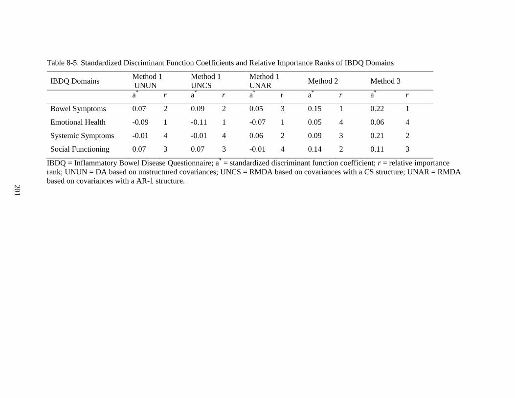
201

Table 8-5. Standardized Discriminant Function Coefficients and Relative Importance Ranks of IBDQ Domains

IBDQ Domains Method 1

UNUN

Method 1

UNCS

Method 1

UNAR Method 2 Method 3

a* r a

* r a

* r a

* r a

* r

Bowel Symptoms 0.07 2 0.09 2 0.05 3 0.15 1 0.22 1

Emotional Health -0.09 1 -0.11 1 -0.07 1 0.05 4 0.06 4

Systemic Symptoms -0.01 4 -0.01 4 0.06 2 0.09 3 0.21 2

Social Functioning 0.07 3 0.07 3 -0.01 4 0.14 2 0.11 3

IBDQ = Inflammatory Bowel Disease Questionnaire; a* = standardized discriminant function coefficient; r = relative importance

rank; UNUN = DA based on unstructured covariances; UNCS = RMDA based on covariances with a CS structure; UNAR = RMDA

based on covariances with a AR-1 structure.

202

8.6 Discussion

This study proposes new methods for evaluating the relative importance of variables in

multivariate repeated measures data. These methods are based on the DFCs derived from stage-

wise RMDA and RMDA procedures in combination with dimension reduction techniques. These

procedures for evaluating the relative importance of variables are advantageous when the sample

size is small relative to the data dimension. Their performance under a variety of data-analytic

conditions was investigated using Monte Carlo techniques and a numeric example was used to

illustrate their application.

Our study results suggests the performance of these methods in correctly rank ordering a

set of variables in multivariate repeated measures design is influenced by the magnitude of

separation between groups, the magnitude of covariance among the variables, and the size of the

outcome variable set. While these procedures differ in their sensitivity to data characteristics,

Method 2, which is based on the SDFCs derived from the average of the within-variable DFCs of

a RMDA procedure that assumes unstructured means and Kronecker product covariances,

maintained the highest any-variable and per-variable correct ranking percentages in almost all

the investigated conditions. While Method 1 was less sensitive to the mean configuration and

correlations among the variables, methods based on the RMDA procedures that assume a

Kronecker product covariance structure (i.e., Methods 2 and 3) were more sensitive to the

configuration of the group means and the magnitude of correlation among the variables. The

percentage of correctly ranked variables for each method decreased as the number of outcome

variables increased.

Moreover, conclusions from the numeric example suggest that bowel symptoms and

emotional health domains are the most important domains that discriminate between active and

203

inactive groups. These findings about the importance of these two IBDQ domains are consistent

with findings from previous studies about the importance of these domains in predicting

longitudinal change in the quality of life of active and inactive disease groups in the IBD

population.

Based on the findings of this study, we recommend that Method 2 be adopted for

evaluating the relative variable importance in multivariate repeated measures data because it

achieved the highest correct ranking rates among the methods investigated. However, previous

research has shown that RMDA procedures may be sensitive to mis-specification of the

covariance structure20,12

, which may in turn influence the rank ordering of variables. We

therefore, recommend that a preliminary evaluation of mean and covariance structure fit such as

log-likelihood ratio test (LRT) be conducted prior to choosing a method. For example, the LRT

developed by Roy and Khattree may be used for testing whether a Kronecker product structure is

a good fit for the data12,31

.

The limitations of these methods for evaluating relative variable importance in

multivariate repeated measures data should be noted. Although previous research notes that

dimension reduction techniques are relatively straightforward to implement, they may result in

loss of information about within-variable temporal trends32

, which may influence the conclusions

about the rank ordering of variables based on the DFCs of RMDA procedures. The simulation

study focused on conditions in which group covariances were equal; this may not be a reasonable

assumption in all data-analytic problems. In addition, complete data were generated for all

measurement occasions. In this study, the SDFC, which is most commonly adopted measure of

relative importance estimated from the DDA model15

, was used to rank order the variables

according to their contribution to group separation. Other measures of relative importance such

204

as the F-to-remove statistic and discriminant ratio coefficients

14,25, which could also be used to

evaluate importance of variables, they were not investigated in this study.

While multivariate repeated measures data are often characterized by observations with

missing data, the methods described in this study assume complete data on all participants and at

each measurement occasion with casewise deletion of observations due to missing data.

However, casewise deletion can result in biased estimates of relative importance when the

mechanism of missingness is not random30

. This is evident in the numeric example where about

24% of the observations have missing values. Although mean imputation method was used to

adjust for missing observations, there are no optimal methods to control bias in the DFC

estimates. Also, multiple imputation30, 33

might be used instead of mean imputation because the

former results in more efficient estimates of the variability than the latter. However,

implementing multiple imputation method for the procedures described in this study may be

computationally intensive. Therefore, the choice between these imputation methods may be

influenced by considerations about the trade-offs between computational burden and accuracy of

parameter estimates.

In summary, this study investigates new methods to evaluate the relative importance of

variables in multivariate repeated measures data. These methods are based on DFCs from

RMDA procedures that assume parsimonious covariance structures. Measures of relative

importance have a number of potential uses for researchers who are interested in studying the

longitudinal change on multiple outcomes. They can be used to identify the set of outcomes that

are most responsive to treatment interventions in longitudinal studies.

205

Acknowledgements


Graduate Scholarship to the first author, and a CIHR New Investigator Award to the second

author.

206

References

1. Keefe, F. J., Dunsmore, J., & Burnett, R. (1992). Behavioral and cognitive–behavioral

approaches to chronic pain: Recent advances and future directions. Journal of Consulting

and Clinical Psychology, 60, 528–536.

2. Soderdahl, D. W., Davis, J. W., Schellhammer, P. F., et al. (2005). Prospective longitudinal

comparative study of health-related quality of life in patients undergoing invasive treatments

for localized prostate cancer. Journal of Endourology, 19, 318 – 326.

3. Perez, D. J., William, S. M., Christensen, E. A., McGee, R. O., & Campbell, A. V. (2001). A

longitudinal study of health-related quality of life and utility measures in patients with

advanced breast cancer. Quality of Life Research, 10, 587 – 593.

4. Boik, R. J. (1991). Scheffe’s mixed model for multivariate repeated measures: A relative

efficiency evaluation. Communication in Statistics, 20, 1233 – 1255.

5. Sheehan-Holt, J. K. (1998). MANOVA simultaneous test procedures: The power and

robustness of restricted multivariate contrasts. Journal of Educational and Psychological

Measurement, 58, 861 – 881.

6. Kim, K., & Timm, N. (2007). Univariate and Multivariate General Linear Models. (2nd

Ed.). Florida: Chapman & Hall/CRC.

7. Lix, L. M., & Sajobi, T. T. (2010). Testing multiple outcomes in repeated measures designs.


8. Lix, L. M., & Sajobi, T. T. (2010). Discriminant analysis for repeated measures data: a

review. Frontiers in Quantitative Psychology and Measurement, 1, 1 – 9.

9. Marshall, G., & Baron, A. E. (2000). Linear discriminant models for unbalanced longitudinal

data. Statistics in Medicine, 19, 1969 – 1981.

207

10. Afifi, A. A., Sacks, S. T., Liu, V. Y., Weil, M. H., & Shubin, H. (1971). Accumulative

prognostic index for patients with barbiturate, glutethimide and meprobamate intoxication.

New England Journal of Medicine, 285, 1497 – 1502.

11. Chang, P. C., Afifi, A. A., Liu, V. Y., Nishijima, H., & Weil, M. H., Shubin, H. (1975).

Prognostic indices for the assessment of patients with Gram-negative bacteremia and shock.

Gram-Negative Bacteria Infections and Mode of Endotoxin Actions – Pathophysiological,

Immunological, and Clinical Aspects, New York: Springer- Verlag.




13. Roy, A., & Khattree, R. (2007). Classification of multivariate repeated measures data with

temporal autocorrelation. Advances in Data Analysis and Classification, 1, 175 – 199.

14. Sajobi, T. T., Lix, L. M., Clara, I., et al. (2012). Measures of relative importance for health-




16. Kivett, V. R., & McCulloch, B. J. (1992). Older rural survivors: Their prediction and

terminal care. Journal of Applied Gerontology, 11, 407 – 424.

17. de Coster, L., Leentjens A. F. G., Lodder, J., & Verhey, F. R. J. (2005). The sensitivity of

somatic symptoms in post-stroke depression: a discriminant analytic approach. International

Journal of Geriatric Psychiatry, 20, 358 – 362.

18. van Tubergen, A., van der Heijde, D., Anderson, J., et al. (2003). Comparison of statistically

derived ASAS improvement criteria for ankylosing spondylitis with clinically relevant

208

improvement according to an expert model. Annals of the Rheumatic Disease, 62, 215 – 221.

19. Levesque, L., Ducharme, F., Zarit, S. H., Lachance, L., & Giroux F. (2008). Predicting

longitudinal patterns of psychological distress in older husband caregivers: further analysis of

existing data. Aging and Mental Health, 12, 333 – 342.

20. Sajobi T. T., Lix L. M., Laverty, W., & Li, L. (in press). Discriminant analysis for repeated

measures data: Effects of covariance misspecification on bias and error in discriminant

function coefficients. Journal of Modern Applied Statistical Methods.



766.

22. Lix, L. M., & Fouladi, R. T. (2007). Robust step-down tests for multivariate independent

group designs. British Journal of Mathematical and Statistical Psychology, 60, 245 – 265.


New Jersey.

24. SAS Institute Inc. (2008). SAS/IML user's guide, version 9.2. SAS Institute, Inc., Cary, North

Carolina.



26. Lix, L. M., & Sajobi, T. T., & Dansu, B. M. A comparison of variable importance measures

for patient reported outcomes. Presented at the International Conference on Health Policy

Statistics, Cleveland, OH, October 5 – 7, 2011.

209

27. Lix, L. M., Graff, L. A., Walker, J. R, L., et al. (2008). Longitudinal study of quality of life

and psychological functioning for active, fluctuating, and inactive disease patterns.

Inflammatory Bowel Diseases, 14, 1575 – 1584.

28. Graff, L. A., Walker, J. R., Lix, L. M., et al. (2006). The relationship of inflammatory bowel

disease type and activity to psychological functioning and quality of life. Clinical

Gastoroenterology and Hepatology, 4, 1491 – 1501.

29. Guyatt, G. H., Mitchell, A., Irvine, E. J., et al. (1989). A new measure of health status for

clinical trials in inflammatory bowel disease. Gastroenterology, 96, 804 – 810.


Ed. New

Jersey: Wiley.

31. Roy, A., & Khattree, R. (2003). Tests for mean and covariance structures relevant in repeated

measures based discriminant analysis. Journal of Applied Statistical Science, 12, 91 – 104.

32. Bandyopadhyay, S., Ganguli, B., & Chatterjee, A. (2011). A review of multivariate

longitudinal data analysis. Statistical Methods in Medical Research, 20, 299 – 330.

33. Roy, A. (2006). A new classification rule for incomplete doubly multivariate data using

mixed effects model with performance comparisons on the imputed Data. Statistics in

Medicine, 25, 1715 – 1728.

210

Appendix I: Estimation of Transformed Discriminant Function Coefficients of

Variable Importance Measures for Multivariate Repeated Measures Discriminant

Analysis Procedures

Let yij be the pq-variate normally distributed multivariate repeated measures data corresponding

to p repeated measurements on each of the q variables in the jth group (i = 1, ..., nj; j = 1, 2; n =

n1 + n2). Assume that yij ~ Npq(μj, Ω), where VΣΩ , Σ is the unstructured between variable

variance-covariance matrix, V is the p×p positive definite compound symmetric structure among

the repeated measurements. The log of the likelihood function l =L(µj1, µj2, Ω| y1j, …,ynj; n = n1 +

n2) is

2

1

1 ))(()((tr2

1||log

22log

2log

j

jijjij

nnpl μyμyVΣVΣ (A-1)

2

1

1 ))(()((tr2

1||log

22log

2log

j

jjjjjj nnnp

l μyμyWVΣVΣ , (A-2)

2

1

1-1- ))(()((tr2

1||log

22log

2log

j

jjjjjj nnnp

l μyμyWVΣVΣ

(A-3)

where Wj = ).()(1

T

jij

n

i

jij

j

yyyy

The ML estimate of μj is obtained by equating the first-order derivatives of equation A-3 to zero.

To obtain the ML estimates of ρ, and Σ, A-3 simplifies to

WVΣVΣ )(2

1||log

2||log

22log

2log 11 tr

nqnpnpql , (A-4)

For a compound symmetric correlation matrix, V,

V = ])1[( T2

ppp 11I , (A-5)

|V| = ,)1]()1(1[ 12 pp p (A-6)

211

and

],)1(1

[)1(

1 T

2

1

pppp

11IV

(A-7)

where where is the common correlation for the repeated measurements, 2 is repeated

measures variance assumed to be constant across measurement occasions, Ip is the pp identity

matrix, 1p is a p×1 vector of ones, V is positive definite, and 11

1

p. Substituting the

values of |V| and V-1

in equations A-6 and A-7 into the log of the likelihood function (equation

A-4) gives

,})1(1){1(2)1(2

||log2

})1(1log{2

)1log(2

)1(2log

2log

21

p

kk

npp

nqqpnnpql Σ

(A-8)

where ,)(tr 1

1 WΣI pk ,)(tr 1

2 WΣJ pk W = W1 + W2, and .T

pp11J

The first order derivative of equation A-8 with respect to ρ and Σ yields

)(})1(2{})1()1()1({)1( 2101

2

2100

3

0 kkkkpkpkpkpkkp , (A-9)

and

T2

1 1 1 1

))((1

jmijm

j

n

i

p

l

p

m

jmijm

lm

j

j

npyyyy-Σ

, (A-10)

where ppnqk )1(0 , ,)(tr 1

1 WΣI pk ,)(tr 1

2 WΣJ pk W = W1 + W2, ,T

pp11J

Ip is a p×p identity matrix, 1p is a p×1 vector of ones, and υlm is the (l,m)th element of V. The ML

estimates of ρ and Σ are obtained by equating A-9 and A-10 to zero and solving the systems of

equations simultaneously.

For Method 2, p

p1C . Then the transformed DFC vector is

212

,))()(( T

21

-1-1TμμVΣCIa

* q (A-11)

T

21

1T-1 ))(( μμVCΣa* . (A-12)

This simplifies to

T

21

T-1 ))(( μμCΣa

* , (A-13)

where

pp

)1(1

1

. (A-14)

For Method 3, C is a p1 vector such that the first and pth elements are 1 and -1, respectively,

while the remaining elements are zero. Then

T

21

T-1 ))(( μμCΣa

* , (A-15)

where

1

1. (A-16)

213

Appendix II: Supplementary SAS Program Documentation

Description

This supplementary documentation contains SAS programming syntax (SAS Institute

Inc., 2008) to illustrate the implementation of methods for evaluating variable importance in

multivariate repeated measures data.

The documentation begins with syntax to read data from a .txt or .dat file into a file

named ‘mrdata’ and a temporary SAS dataset called ‘mrmappendix’. If the data are not in a .txt

or .dat file, then the syntax at the beginning of the program will change. Consult your SAS user’s

manual or contact the authors if you require assistance to prepare your dataset for use.

This documentation demonstrates the SAS syntax for multivariate repeated measures data

that contains three outcome variables that were measured at 3 measurement occasions. The data

for first variable for the three measurement occasions are named y11, y12, and y13, respectively.

The data for the second outcome variable for the three measurement occasions are named y21,

y22, and y23, respectively. The data for the third outcome variable are named y31, y32, and y33,

respectively. The data also contain the numeric variable grp, which is used to discriminate

between the two study groups. The grp variable takes on values of 0 and 1. In this example, there

are 54 observations (i.e., individuals) in group 1 and 76 observations in group 2. The group sizes

must be specified in the SAS program.

The components of the program that require user input are highlighted in boldface font.

The program will generate an error if there are missing data for any of the variables in the

dataset.

Reference

SAS Institute Inc. (2008). SAS/IML user's guide, version 9.2. Cary, NC: SAS Institute Inc.

214

**Read in the data**;

filename mrmdata 'Note to users: the dataset path and filename is inserted between the single

quotation marks';

data mrmappendix;

infile mrmdata;

input grp y11 y12 y13 y21 y22 y23 y31 y32 y33;

run;

**Use the IML procedure to read the dataset and its specifications**;

proc iml;

use mrmappendix;

read all var { y11 y12 y13 y21 y22 y23 y31 y32 y33} into y;

read all var {grp} into x;

knum = 3; lnum = 3;

dv = knum#lnum;

grpsz1 = 54; grpsz2 = 76;

c1 = {1 1 1}/3;

c2 = {1 0 -1}/3;

/*********************************************************************

Module Name: stagewiseda

Module Output:

sdfc: Standardized discrimiant function coefficients based on UNUN Procedure

rsdfc1: Variable Ranking based on sdfc1

*********************************************************************/

start stagewise_unun(y,knum,lnum, grpsz1,grpsz2,dv,dcoef1, ddcoef1,sdfc1, rsdfc1);

215

one = j(dv,1, 1); n = nrow(y);

dfs = J(n, knum,0); adc = J(1,knum,0);

dcoef1 = J(lnum, knum, 0); dcoef = J(lnum, knum, 0);

gp1 = y[1: grpsz1, ]; gp2 = y[(grpsz1+1):n, ];

ybar1 = gp1[+,]/grpsz1; ybar2 = gp2[+,]/grpsz2;

ss1 = J(dv,dv,0); ss2 = J(dv,dv,0);

do i = 1 to grpsz1;

ss1 = ss1+ (gp1[i,]- ybar1)`*(gp1[i,]- ybar1);

end;

do i = 1 to grpsz2;


end;

sig = (ss1 +ss2)/(n-1);

/***Estimate DFCs for data on each variable (Stage 1)*****/

do m = 1 to knum;

dcoef1[,m] = inv(sig[(((m-1)*lnum)+1): (m*lnum), (((m-1)*lnum)+1): (m*lnum)])*(

(ybar1[,(((m-1)*lnum)+1): m*lnum]) - (ybar2[,(((m-1)*lnum)+1): m*lnum]))`;

adc[,m]= sqrt((dcoef1[,m])`*(sig[(((m-1)*lnum)+1): (m*lnum), (((m-1)*lnum)+1):

(m*lnum)])*dcoef1[,m]);

dcoef[,m]=(dcoef1[,m])/adc[,m];

dfs[,m] = y[,(((m-1)*lnum)+1):(m*lnum)]*dcoef[,m];

end;

/**Compute Discriminant function Scores for each variable based on DFCs in Stage 1****/

216

dfs1 = dfs[1:grpsz1,]; dfs2 = dfs[(grpsz1 + 1): n, ];

dfbar1 = dfs1[+,]/grpsz1; dfbar2 = dfs2[+,]/grpsz2;

/***Estimate DFCs based on the discriminant function scores (Stage 2) *****/

dss1 = J(knum,knum,0); dss2 = j(knum,knum, 0);

do i = 1 to knum;

dss1 = dss1+ (dfs1[i,]- dfbar1)`*(dfs1[i,]- dfbar1);


end;

dsig = (dss1 +dss2)/(n-2);

ddcoef1 = inv(dsig)*(dfbar1 - dfbar2)`;

dadc =(ddcoef1`*(dsig)*ddcoef1);

sddcoef1 = ddcoef1/dadc;

****Compute SDFCs and Variable Ranks***;

sdfc1 = J(knum,1,0);

do k = 1 to knum;

sdfc1[k] = sddcoef1[k]*sqrt(dsig[k,k]);

end;

rsdfc1 = knum-ranktie(abs(sdfc1))+1;

finish stagewise_unun;

/***************************************************************************

Module Name: stagewise_uncs

Module Output:

sdfc2: Standardized discrimiant function coefficients based on UNCS Procedure

217


*************************************************************************/

start stagewise_uncs(y,knum, lnum,grpsz1, grpsz2, dv, ddcoef2, sdfc2, rsdfc2);

n = nrow(y);

dcoef2 = J(lnum, knum, 0); dcoef22 = J(lnum, knum, 0);

dcoef = J(lnum, knum, 0); dfs = J(n,knum,0); adc2 = J(1,knum,0);

ybard = J(1,dv,0); msigm = J(dv,dv,0); ybar = y[+,]/n;




do i = 1 to grpsz1;


end;

/****Estimate the ML Estimates of CS covariance parameters for Repeated Measurements on

Each Variable***/

do i = 1 to grpsz2;


end;

sig1 = ss1/(grpsz1-1); sig2 = ss2/(grpsz2-1);

w = (ss1 +ss2)/(n-1);

jn = J(lnum,lnum,1);

a8 = J(1,knum, 0); a9 = J(1,knum, 0); b8 = J(1,knum, 0); b9 = J(1,knum, 0);

k0 = J(1,knum,0); pp = J(1,knum,0); qq = J(1,knum,0); rr = J(1,knum,0); aa = J(1,knum,0); bb

218

= J(1,knum,0);

d = J(1,knum,0); s1 = J(1,knum,0); s2 = J(1,knum,0); s3= J(1,knum,0); ar = J(1,knum,0); ar1 =

J(1,knum,0); ar2= J(1,knum,0);

mrho1= J(1,knum,0); mrho2 = J(1,knum,0); abr1= J(1,knum,0);

msig = J(1,knum,0); msige = J(1,knum,0); au = J(1,knum,0);

do m = 1 to knum;

ym = y[, (((m-1)*lnum)+1): m*lnum];

ybard[,(((m-1)*lnum)+1): m*lnum] = (ybar1[,(((m-1)*lnum)+1): m*lnum]) - (ybar2[,(((m-

1)*lnum)+1): m*lnum]);

mybar = ybar[, (((m-1)*lnum)+1): m*lnum];

w1 = sig1[(((m-1)*lnum)+1): (m*lnum), (((m-1)*lnum)+1): (m*lnum)];

w2 = sig2[(((m-1)*lnum)+1): (m*lnum), (((m-1)*lnum)+1): (m*lnum)];

a8[,m] = trace(w1); a9[,m] = trace(w2); b8[,m] = trace(jn*w1); b9[,m] = trace(jn*w2);

mybarn = repeat(mybar,n,1);

mgp = ym - mybarn;

mgpass = mgp[##,];

msq_gp = repeat(sqrt(mgpass),n,1);

mgpa = mgp/msq_gp;

S = t(mgpa)*(mgpa);

mrho1[,m] = (s[+,+] - trace(s))/(lnum*(lnum-1));


iter = 0; converge = 0.00001;

msig[,m] = ((1 + (lnum-1)*mrho1[,m])*(a8[,m]+a9[,m]) - mrho1[,m]*(b8[,m]+b9[,m]))/

219

(n*lnum*(1-mrho1[,m])*(1 + (lnum-1)*mrho1[,m]));

absig = abs(msige[,m] - msig[,m]);

msige[,m] = msig[,m];

k0[,m] = n*(lnum-1)*lnum*msig[,m];

pp[,m] = -((lnum-2)*k0[,m] - ((a8[,m]+a9[,m])*(lnum-1)**2) + (b8[,m]+b9[,m])*(lnum-

1))/((lnum-1)*k0[,m]);

qq[,m] =-(k0[,m] - 2*(a8[,m]+a9[,m])*(lnum-1))/((lnum-1)*k0[,m]);

rr[,m] = -(b8[,m]+b9[,m] - a8[,m] - a9[,m])/((lnum-1)*k0[,m]);

aa[,m] = (1/3)*(3*qq[,m]-pp[,m]**2);

bb[,m] = (1/27)*(2*pp[,m]**3 - 9*pp[,m]*qq[,m] + 27*rr[,m]);

d[,m] = (bb[,m]**2)/4 + (aa[,m]**3)/27;

if d[,m] < 0 then s1[,m] = 0;

else s1[,m] = d[,m]**0.5;

au[,m] = -bb[,m]/2 + s1[,m];

if au[,m] < 0 then s2[,m] =0;

else s2[,m] = (au[,m])**(1/3);

ar[,m] = -bb[,m]/2 - s1[,m];

if ar[,m] < 0 then do;

ar1[,m] = -ar[,m];

ar2[,m] = ar1[,m]**(1/3);

s3[,m] = -ar2[,m];

end;

else do;

220

s3[,m] = ar[,m]**(1/3);

end;

mrho2[,m] = s2[,m] + s3[,m] - pp[,m]/3;

iter = iter +1;

abr1[,m] = abs(mrho1[,m] - mrho2[,m]);

mrho1[,m] = mrho2[,m];

maxab = max(absig//abr1[,m]);

end;

msigm[(((m-1)*lnum)+1): (m*lnum), (((m-1)*lnum)+1): (m*lnum)] = (msig[,m])*( (1-

mrho2[,m])*i(lnum) + mrho2[,m]*jn);

end;

***Compute the DFCs and Discriminant Function Scores for Each Variable (Stage 1);

do m = 1 to knum;

dcoef2[,m] = inv(msigm[(((m-1)*lnum)+1): (m*lnum), (((m-1)*lnum)+1):

(m*lnum)])*(ybard[,(((m-1)*lnum)+1): m*lnum])`;

adc2[,m]= sqrt((dcoef2[,m])`*(msigm[(((m-1)*lnum)+1): (m*lnum), (((m-1)*lnum)+1):


dcoef22[,m]=(dcoef2[,m])/adc2[,m];

dfs[,m] = y[,(((m-1)*lnum)+1):(m*lnum)]*dcoef2[,m];

end;

dfs1 = dfs[1:grpsz1,];

dfs2 = dfs[(grpsz1 + 1): n, ];

dfbar1 = dfs1[+,]/grpsz1;

221

dfbar2 = dfs2[+,]/grpsz2;

/***Estimate DFCs based on the discriminant function scores (Stage 2)*/


do i = 1 to knum;



end;



dadcd = (ddcoef2`*(dsig)*ddcoef2);

ddcoef2_t = ddcoef2/dadcd;



do k = 1 to knum;

sdfc2[k] = ddcoef2_t[k]*sqrt(dsig[k,k]);

end;


finish stagewise_uncs;

/*************************************************************************

Module Name: stagewise_unar

Module Output:

sdfc3: Standardized discrimiant function coefficients based on UNAR Procedure


222

*************************************************************************/

start stagewise_unar(y,knum, lnum,grpsz1, grpsz2, dv,ddcoef3, sdfc3, rsdfc3);

n = nrow(y); dcoef3 = J(lnum, knum, 0);

dcoef33 = J(lnum, knum, 0); dfs = J(n,knum,0);

adc3 = J(1,knum,0); ybard = J(1,dv,0); msigm = J(dv,dv,0); ybar = y[+,]/n;




/****Estimate the ML Estimates of CS covariance parameters for Repeated Measurements on

Each Variable***/

do i = 1 to grpsz1;


end;

do i = 1 to grpsz2;


end;

sig1 = ss1/(grpsz1-1); sig2 = ss2/(grpsz2-1);

ws = (ss1 + ss2);

gama1 = J(1, knum, 0); jn = J(lnum,lnum,1);

beta1 = J(1, knum, 0); a1 = J(1,knum, 0); a9 = J(1,knum, 0);

b8 = J(1,knum, 0); b9 = J(1,knum, 0);

k0 = J(1,knum,0); pp = J(1,knum,0); qq = J(1,knum,0); rr = J(1,knum,0); aa = J(1,knum,0); bb

= J(1,knum,0);

223

d = J(1,knum,0); s1 = J(1,knum,0); s2 = J(1,knum,0); s3= J(1,knum,0); ar = J(1,knum,0); ar1 =

J(1,knum,0); ar2= J(1,knum,0);

mrho1= J(1,knum,0); mrho2 = J(1,knum,0); abr1= J(1,knum,0);

msig = J(1,knum,0); msige = J(1,knum,0); au = J(1,knum,0);

do m = 1 to knum;

ym = y[, (((m-1)*lnum)+1): m*lnum];

ybard[,(((m-1)*lnum)+1): m*lnum] = (ybar1[,(((m-1)*lnum)+1): m*lnum]) - (ybar2[,(((m-

1)*lnum)+1): m*lnum]);

mybar = ybar[, (((m-1)*lnum)+1): m*lnum];

w = ws[((m-1)*lnum+1) : m*lnum, ((m-1)*lnum+1) : m*lnum];

a1[,m] = trace(w);

beta1[,m] = trace(w) - w[1,1] - w[lnum,lnum];

do i = 1 to lnum-1;

gama1[,m] = gama1[,m] + w[i,i+1];

end;

mybarn = repeat(mybar,n,1);

mgp = ym - mybarn;

mgpass = mgp[##,];

msq_gp = repeat(sqrt(mgpass),n,1);

mgpa = mgp/msq_gp;

s = t(mgpa)*(mgpa);

mrho1[,m] = (s[+,+] - trace(s))/(lnum*(lnum-1));


224

iter = 0; converge = 0.000001;

msig[,m] = (beta1[,m]*mrho1[,m]**2 - (2*gama1[,m]*mrho1[,m]) + a1[,m])/(n*lnum*(1-

mrho1[,m]**2));

msige[,m] = msig[,m];

absig = abs(msige[,m] - msig[,m]);

pp[,m] = -(gama1[,m]) /(n*(lnum-1)*msig[,m]);

qq[,m] =-(n*(lnum-1)*msig[,m] - (a1[,m]+beta1[,m]))/(n*(lnum-1)*msig[,m]);

rr[,m] = -(gama1[,m])/(n*(lnum-1)*msig[,m]);

aa[,m] = (1/3)*(3*qq[,m]-pp[,m]**2);

bb[,m] = (1/27)*(2*pp[,m]**3 - 9*pp[,m]*qq[,m] + 27*rr[,m]);

d[,m] = (bb[,m]**2)/4 + (aa[,m]**3)/27;

if d[,m] < 0 then s1[,m] = 0;

else s1[,m] = d[,m]**0.5;

au[,m] = -bb[,m]/2 + s1[,m];

if au[,m] < 0 then s2[,m] =0;

else s2[,m] = (au[,m])**(1/3);

ar[,m] = -bb[,m]/2 - s1[,m];

if ar[,m] < 0 then do;

ar1[,m] = -ar[,m];

ar2[,m] = ar1[,m]**(1/3);

s3[,m] = -ar2[,m];

end;

else do;

225

s3[,m] = ar[,m]**(1/3);

end;

mrho2[,m] = s2[,m] + s3[,m] - pp[,m]/3;

iter = iter +1;

abr1[,m] = abs(mrho1[,m] - mrho2[,m]);

mrho1[,m] = mrho2[,m];

maxab = max(absig//abr1[,m]);

end;

v = J(lnum, lnum, 0);

do i = 1 to lnum;

do j = 1 to lnum;

v[I,J] = msig[,m]*mrho2[,m]**(abs(i-j));

end;end;

msigm[(((m-1)*lnum)+1): (m*lnum), (((m-1)*lnum)+1): (m*lnum)] = v;

end;

***Compute the DFCs and Discriminant Function Scores for Each Variable (Stage 1);

do m = 1 to knum;

dcoef3[,m] = inv(msigm[(((m-1)*lnum)+1): (m*lnum), (((m-1)*lnum)+1):

(m*lnum)])*(ybard[,(((m-1)*lnum)+1): m*lnum])`;

adc3[,m]= sqrt((dcoef3[,m])`*(msigm[(((m-1)*lnum)+1): (m*lnum), (((m-1)*lnum)+1):


dcoef33[,m]=(dcoef3[,m])/adc3[,m];

dfs[,m] = y[,(((m-1)*lnum)+1):(m*lnum)]*dcoef3[,m];

226

end;

dfs1 = dfs[1:grpsz1,]; dfs2 = dfs[(grpsz1 + 1): n, ];

dfbar1 = dfs1[+,]/grpsz1; dfbar2 = dfs2[+,]/grpsz2;

/**Compute Discriminant function Scores for each variable based on DFCs in Stage 1*/


do i = 1 to knum;



end;



dadcd3 = (ddcoef3`*(dsig)*ddcoef3);

ddcoef3 = ddcoef3/dadcd3;



do k = 1 to knum;

sdfc3[k] = ddcoef3[k]*sqrt(dsig[k,k]);

end;


finish stagewise_unar;

/****************************************************************************

Module Name: mrmda

227

Module Output:

sdfc4: Standardized discrimiant function coefficients for Method 2


sdfc5: Standardized discrimiant function coefficients for Method 3


*****************************************************************************/

start mrmda (y, knum, lnum, grpsz1, grpsz2, dv, c1, c2, tdcoef, sdfc4, sdfc5,rsdfc4, rsdfc5);

n = nrow(y);

mdcoef = J(dv, 1, 0);

one = J(lnum,1,1);

ybar = y[+,]/n;


ybar1 = gp1[+,]/grpsz1;

ybar2 = gp2[+,]/grpsz2;

w = J(dv,dv,0);

/***ML Estimation of Kronecker product covariance parameters (i.e, V and Sigma)*/

do i = 1 to n;

w = w + (y[i,]- ybar)`*(y[i,]- ybar);

end;

mya = J(n,dv,0);

do i =1 to n;

mya[i,] = y[i,] - ybar;

end;

228

yass=mya[##, ];

sq_assm= repeat(sqrt(yass),n,1);

yan=mya/sq_assm;

v0=t(yan)*yan;

vi = J(knum, knum, 0);

do k = 1 to lnum;

vi = vi + v0[((k-1)*knum+1): k*knum, ((k-1)*knum+1): k*knum];

end;

vi=vi/knum;

rest= (vi[+,+]-trace(vi))/(lnum*(lnum-1));

ve=(1-rest) *I(lnum) + rest#(one*t(one));

jj = I(lnum); v = J(lnum,lnum,0);

tau = I(lnum) @ I(knum);

/* Calculating the mle's mlv and mlsig of V and Sigma.*/

mlsige=j(knum,knum,0); iter=0; converge = 0.001;

do until (maxab<converge);

ive=inv(ve);

do l = 1 to lnum;

do m = 1 to lnum;

v[l,m] = t(jj[,l])*ive*jj[,m];

end;end;

sigma_e=j(knum,knum,0);

subba = J(n,dv, 0);

229

subb = J(n, dv, 0);

do i = 1 to n;

subba[i, ]= y[i,] - ybar;

end;

do k = 1 to lnum;

subb[,((k-1)*knum)+1 : k*knum] = t(tau[((k-1)*knum)+1 : k*knum, ]* t(subba));

end;

do l = 1 to lnum;

do m = 1 to lnum;

sigma_e = sigma_e + v[l, m]*(t(subb[,((m-1)*knum)+1 : m*knum])* subb[, ((l-1)*knum)+1 :

l*knum]);

end; end;

mlsig=sigma_e/(n*lnum);

absig=abs(trace(mlsige-mlsig));

mlsige=mlsig;

imlsig=inv(mlsig);

k3=trace((I(lnum)@imlsig)*w);

k4=trace(((one*t(one))@imlsig)*w);

s=lnum-1; ko=n*knum*s*lnum;

pp=(ko-s*ko+(k3*s**2)-s*k4)/(s*ko); qq=(2*s*k3-ko)/(s*ko); rr=(k3-k4)/(s*ko);

aa=(1/3)*(3*qq-pp**2); bb=(1/27)*(2*pp**3 -9*pp*qq + 27*rr);

discrim=(abs(bb)**2)/4+(abs(aa)**3)/27;

if discrim > 0 then do;

230

s1 = (discrim)**0.5;

end;

else do;

s1 =0;

end;

sn = -bb/2+ s1;

if sn > 0 then do;

s2=(sn)**(1/3);

end;

else do;

s2 = (abs(sn))**(1/3);

end;

ar=-(bb/2)- s1;

if ar <0 then

do;

ar1=-ar; ar2=ar1**(1/3); s3=-ar2;

end;

else

do;

s3=ar**(1/3);

end;

ro2=abs(s2+s3-(pp/3));

mlv=(1-ro2)*I(lnum)+ro2*one*t(one);

231

ve=mlv;

iter=iter+1;

abr1=abs(rest-ro2);

rest=ro2;

maxab=max(absig//abr1);

end;

omega = mlsig @ ve;

****Compute overall DFCs and its linear transformation based on c1 and c2**;

mdcoef = inv(omega) *(ybar1 - ybar2)`;

madc = sqrt(abs(mdcoef`*omega*mdcoef));

mdcoef = mdcoef/madc;

m1 = i(knum)@c1;

m2 = i(knum)@c2;

tdcoef1 = m1*mdcoef;

tdcoef2 = m2*mdcoef;

tomega1 = m1*omega*m1`;

tomega2 = m2*omega*m2`;

****Compute transformed SDFCs and Variable Rankings***;


do k = 1 to knum;

sdfc4[k] = tdcoef1[k]*sqrt(abs(tomega1[k,k]));

end;

232



do k = 1 to knum;

sdfc5[k] = tdcoef2[k]*sqrt((tomega2[k,k]));

end;


finish mrmda;

call stagewise_unun(y,knum,lnum, grpsz1,grpsz2,DV,dcoef1,ddcoef1, sdfc1, rsdfc1);

call stagewise_uncs(y,knum, lnum,grpsz1, grpsz2, dv, ddcoef2, sdfc2,rsdfc2);

call stagewise_unar(y,knum, lnum,grpsz1, grpsz2, dv, ddcoef3, sdfc3, rsdfc3);

call mrmda (y, knum, lnum, grpsz1, grpsz2, dv, c1, c2, tdcoef, sdfc4, sdfc5,rsdfc4, rsdfc5);

Print 'Vector of SDFC for stagewise RMDA-UNUN procedure (Method 1) ;' sdfc1[format =8.2];

Print 'Vector of Variable Rank DFCs for SDFCs based on Stagewise RMDA(Method 1) ;'

rsdfc1[format =8.2];

Print 'Vector of SDFCs for stagewise RMDA procedure based on UNCS procedure(Method 1) ;'

sdfc2[format =8.2];

Print 'Vector of Variable Rank DFCs for SDFCs derived from Stagewise RMDA-UNCS

procedure(Method 1) ;' rsdfc2[format =8.2];

Print 'Vector of SDFCs for stagewise RMDA-UNAR procedure(Method 1);' sdfc3[format =8.2];

Print 'Vector of Variable Rank DFCs based on SDFCs of Stagewise RMDA-UNAR

procedure(Method 1);' rsdfc3[format =8.2];

Print 'Vector of SDFCs for transformed SDFCs of RMDA procedure that assume Kronecker

product covariance (Method 2);' sdfc4[format =8.2];

233

Print 'Vector of Variable Ranks for transformed SDFCs of RMDA procedure that assume

Kronecker product covariance (Method 2);' rsdfc4[format =8.2];

Print 'Vector of SDFCs for transformed SDFCs of RMDA procedure that assume Kronecker

product covariance (Method 3);' sdfc5[format =8.2];

Print 'Vector of Variable Ranks for transformed SDFCs of RMDA procedure that assume

Kronecker product covariance (Method 3);' rsdfc5[format =8.2];

quit;

234

Chapter 9. Discussion and Conclusions

Abbreviations






IBD = Inflammatory bowel disease

IBDQ = Inflammatory Bowel Disease Questionnaire

LR = Logistic regression

MAR = Missing at random

MNAR = Missing not at random


MSE = Mean square error


RMSE = Root mean square error


235

9.1 Summary

The objectives of this research were to develop descriptive discriminant analysis (DDA)

procedures based on parsimonious covariance structures that are also insensitive to non-

normality in repeated measures data and to develop techniques based on repeated measures DDA

procedures for evaluating the relative importance of variables that discriminate between groups

in multivariate repeated measures data.

Repeated measures discriminant analysis (RMDA) procedures that assume parsimonious

covariance structures (and possibly even parsimonious mean structures) have been developed

based on growth curve, mixed-effects, and covariance structure models1 for classifying

observations in univariate and multivariate repeated measures data. As Huberty and Wisenbaker2

note, discriminant analysis (DA) procedures can also be used to identify the relative importance

of variables for discriminating between groups. There has been little, if any research on the topic

of DDA for repeated measures data.

This dissertation begins by investigating RMDA procedures based on covariance

structure models for describing group separation in univariate repeated measures data. The bias

and error in the discriminant function coefficients (DFCs) of RMDA procedures that assume

parsimonious covariance structures were investigated under a variety of data-analytic conditions

using Monte Carlo methods. Bias in the DFCs was influenced by mis-specification of the

covariance structure of the data. The magnitude of bias due to mis-specification was largest

under normally distributed data, but it was attenuated for multivariate non-normal data. As

expected, mean square error (MSE) was smallest for all procedures when the covariance was

correctly specified and largest when it was mis-specified. The effect of mis-specification on the

errors of the DFCs was attenuated when the data were multivariate non-normal. Parsimony of the

236

covariance structure resulted in smaller error but larger bias in the DFCs estimates. The DFCs of

the linear DA procedure that assumes unstructured covariances was less biased but also less

efficient.

Robust RMDA procedures that are insensitive to departures from the assumption of

multivariate normality were developed for describing group separation in non-normal data.

These robust RMDA procedures were developed based on coordinatewise trimming (CT) of the

repeated measures data and applying maximum likelihood (ML) estimators to the trimmed data.

The CT approach was adopted because of its computational simplicity and good theoretical

properties that have been demonstrated in previous research for multivariate data. The DFCs of

these procedures were less biased than the DFCs of the RMDA procedures based on ML

estimators for untrimmed data. The impact of mis-specification of the covariance structure on

bias in the DFCs of robust RMDA procedures was smaller than for RMDA procedures based on

ML estimators when the data were sampled from non-normal distributions.

The root mean square error (RMSE) of the estimated DFCs was influenced by the

population distribution, covariance structure, and mean structure. The DFCs of robust RMDA

procedures that did not place any restrictions on the group means were more efficient (i.e.,

smaller RMSE) than the DFCs of the corresponding procedures based on ML estimators when

the population covariance structure was mis-specified. Error in the DFCs increased as the

magnitude of the correlation among the repeated measurements.

New measures of relative importance based on DFCs from RMDA procedures were

developed for identifying the variables that discriminate between groups in multivariate repeated

measures data. These new measures are the standardized discriminant function coefficients

(SDFCs) based on a stage-wise RMDA procedure and linear transformations of the DFCs of a

237

multivariate RMDA procedure that assumes a Kronecker product covariance covariance

structure. Statistical derivations about the equivalence of variable ranks for based on SDFCs

obtained from linear transformation of the DFCs of the RMDA procedures and variable ranks

based on SDFCs obtained from linear transformations of the variables were provided. A

comparison of these methods using Monte Carlo techniques suggests that SDFCs based on the

average of within-variable DFCs of a RMDA procedure with a Kronecker product covariance

structure resulted in the highest proportion of correctly ranked variables among the investigated

procedures. However, the proportion of correctly ranked variables was sensitive to data-analytic

characteristics, including the magnitude of separation between the group means, the structure and

magnitude of correlation among the outcomes, and the number of study variables. This finding

was also demonstrated in the numeric example, where there were disimilarities in the rank order

of inflammatory bowel disease (IBDQ) domains from different relative importance measures.

9.2 Discussion

Mis-specification of the covariance structure for DA procedures results in reduced

classification accuracy3-4

. The current research has shown that covariance mis-specification can

also result in increased bias and error in the DFCs of RMDA procedures. While conventional

RMDA procedures are sensitive to departures from a multivariate normal distribution, the

proposed robust RMDA procedures resulted in reduced bias and error in non-normal

distributions. The DFCs of RMDA procedures based on coordinatewise trimming (CT) of the

non-normal data were less biased and more efficient than those of RMDA procedures based on

ML estimators under strong departures from multivariate normal distribution. For moderately

skewed and or heavy-tailed distribution, the DFCs of the former procedures were similar to those

of the latter procedures. However, it is important to note that there were no disadvantages

238

associated with using robust RMDA procedures when the data were normally distributed. These

findings are consistent with previous research showing that trimmed means and Winsorized

estimators perform equally well under normally distributed data and small sample sizes5. Thus,

robust RMDA procedures should be routinely used because they can offer distinct advantages

when the data demonstrate significant departures from multivariate normality.

Our findings about bias and error in the DFCs of RMDA procedures that assume

parsimonious covariance structures are consistent with previous research findings6-7

. Adopting a

DA procedure based on a simplified covariance structure will substantially reduce the number of

parameters to estimate, but bias in the parameter estimates can sometimes be large and will

increase as the degree of deviance between the model and the data increases. A researcher’s

choice of a DA procedure for repeated measures data is dependent, in part, on the trade-off

between parsimony and bias and/or error in the DFCs when describing differences between

groups.

Data characteristics such as the magnitude of separation between group means and

magnitude and pattern of correlation among the variables influenced the proposed methods for

evaluating variable importance in multivariate repeated measures data. These results corroborate

previous findings about the sensitivity of measures of relative importance to a variety of data

analytic conditions8-9

. However, a mis-specification of the within-variable correlation structure

did not have a large influence on the ability of the proposed methods to correctly rank order the

variables according to their contributions to group separation in multivariate repeated measures

data. This might be attributed to the fact that the proposed methods adopt dimension reduction

techniques to summarize within-variable measurements on each variable. Previous research has

shown that while dimension reduction techniques are straightforward to implement, they may

239

result in some loss of information about the temporal trends in the data10

.

Data from the Manitoba Inflammatory Bowel Disease (IBD) Cohort Study11

were used to

illustrate the application of robust RMDA procedures for describing group separation (Chapter

6). It was also used to illustrate the application of methods for evaluating the relative importance

of variables in multivariate repeated measures data (Chapter 8). The choice of this dataset for the

numeric examples was motivated by its characteristics, namely (a) moderate to strong

correlations among the domains, (b) high-dimensional data for multiple domains and

measurement occasions, and (c) moderate to extreme departures from multivariate normality

assumptions. Through the numeric examples, software to implement the procedures was

presented. This detailed information on the application of the proposed procedures can benefit

applied statisticians as well as clinicians who will implement the proposed methods in their own

research. Our analysis suggests that the IBD Questionnaire (IBDQ) bowel symptoms and

emotional health domains were the most important domains that discriminated between active

and inactive disease groups within the first two years of the study. These findings are consistent

with previous research based on data collected at study baseline12

.

9.3 Research Strengths and Limitations

This research has a number of strengths. The robust RMDA procedures developed in this

study are based on CT of the repeated measures data, which is straightforward to implement.

This estimation method, which replaces the conventional mean and covariance with trimmed

means and Winsorized covariances, possesses good theoretical properties in both skewed and

heavy-tailed distributions13

. Another advantage of this robust estimation approach is that

observations considered to be “outliers” with respect to some coordinates are not completely

eliminated from the sample, which preserves information on the non-outlying coordinates15

.

240

To evaluate the relative importance of variables in multivariate repeated measures data,

DFCs from the RMDA procedures were used in combination with dimension reduction

techniques to rank variables according to their contribution to group separation. These proposed

methods for evaluating relative importance of variables in multivariate repeated measures data

are intuitively appealing, easy to implement, and are advantageous when the sample size is small

relative to the data dimension10

. In addition, the methods described in this study were also found

to be less sensitive to mis-specification of the covariance structure for multivariate repeated

measures data.

However, the limitations of this research should be noted. An assumption that underlies

the methods investigated in this research is homogeneity of group covariances. This assumption

may not always be satisfied in clinical studies in which there is more variability in the treatment

group than the control group16

. Previous research has shown that the conventional DA procedure

based on least squares estimators is less sensitive to heterogeneity of group covariances when the

data are normally distributed and more sensitive to heterogeneity in non-normal distributions17

.

Quadractic DA procedures that allow for heterogeneity in group covariances have been

developed for repeated measures data, but their emphasis is on prediction and not description.

The impact of group covariance heterogeneity on the ranking accuracy of the investigated

procedures is not known for multivariate non-normal data.

The investigated RMDA procedures assume complete data on all observations and across

repeated measurements, with casewise deletion of observations occurring when there is missing

data. However, casewise deletion may result in biased estimates of DFCs when the mechanism

of missingness is not random18

and loss of statistical power due to smaller sample size.

The DFCs of RMDA procedures can be used to evaluate the importance of

241

variables/measurement occasions in discriminating between groups. However, sample statistics

cannot be generalized to the population. Inferential methods for DFCs and the corresponding

ranks have been proposed and could also be applied to repeated measures data. For example,

Huberty and Wisenbaker2 adopted bootstrap methods to test whether DFCs are significantly

different from zero. A recent paper on statistical inference for relative importance measures was

proposed by our research group, but was beyond the scope of this dissertation19

.

The conclusion that one variable is more important than another variable can only be

applied to the set of variables under investigation. Therefore, changing the mix of variables

included in a study could change a researcher’s conclusions about variable importance2. Finally,

variable selection techniques were not applied to the data prior to conducting DDA20-21

. It is

assumed that the set of variables are determined a priori and selected based on theoretical

considerations. This is a reasonable approach in the analysis of multi-dimensional HRQOL data,

where researchers are unlikely to have a plan to exclude some domains from the analysis.

9.4 Future Research

This research study have focused on the development of repeated measures DDA

procedures and their application in evaluating variable importance in multivariate repeated

measures data. Topics for future investigations in this topic area are numerous. These include the

development of robust RMDA procedures for evaluating variable importance in multivariate

repeated measures data characterized by non-normal distributions, non-ignorable missing data,

and/or measurement error. As well, statistical inference about variable importance measures also

represents an area for further exploration.

While robust RMDA procedures have been developed based on the CT estimation

method for repeated measures data, further research could investigate high breakdown robust

242

estimators for describing group separation in multivariate repeated measures data, including

minimum covariance determinant estimators and trimmed likelihood estimation methods22-23

,

which have been proposed for developing robust maximum likelihood estimators of means and

covariances. Unlike the CT estimation which independently trims the data on each measurement

occasion separately, these highbreakdwon estimators are advantageous because they account for

both within-variable and between-variable correlations among the variable in developing robust

estimators of means and covariances24, 25

.

An assumption underlying the methods in the dissertation is that the outcome variables

are measured without error. However, this assumption may not be tenable in longitudinal health-

related quality of life (HRQOL) studies where proxy measurements may be obtained for study

participants who are unable to self-report their quality of life. Previous research has shown that

the presence of measurement error in variables may influence the classification accuracy of the

DA classification rule and result in incorrect rank ordering of the variables that discriminate

between groups26

. One method to address measurement error in discriminant analysis models is

the moment reconstruction method, a form of regression calibration for logistic regression27

.

However, there is limited investigation about methods for correcting measurement error in

continuous variables when adopting RMDA procedures.

The methods used to evaluate the relative importance of variables in multivariate

repeated measures data rests on the assumption of multivariate normality. The sensitivity of these

procedures to multivariate non-normal repeated measures data has not been investigated.

Although robust RMDA procedures based on CT have been proposed in this study, the extension

of these procedures to multivariate repeated measures data has not been investigated. Such

procedures are particularly relevant for evaluating variable importance in non-normal

243

multivariate repeated measures data. Further research will investigate whether the CT approach

is unbiased and efficient when each repeated measurement on each variable is trimmed

separately and then a linear combination of the observations is created. The application of this

robust procedure for evaluating the relative importance of variables in multivariate non-normal

repeated measures data will also be investigated.

In two-group repeated measures studies there is only one statistically significant

discriminant function. However, for multi-group designs, more than one statistically significant

discriminant function may exist; consequently the assessment of variable importance may not be

straightforward. Huberty and Wisenbaker2 proposed using a weighted linear combination of the

DFCs on each variable to evaluate variable importance in multi-group designs. Further research

is needed to develop this approach for constructing relative importance measures in multi-group


The RMDA procedures developed in this study do not accommodate missing

observations. Previous research has investigated RMDA procedures based on multiple

imputation methods and mixed-effects models when the data are characterized by missing

observations20

. The RMDA procedure based on the mixed-effects model, which classifies

observations into groups based on their subject-specific means and covariances28-30

, have been

shown to result in better classification accuracy than the conventional DA procedure based on

multiply imputed data, when the missing data are assumed to be missing at random (MAR).

RMDA procedures based on mixed-effects models can also accommodate unbalanced repeated

measures data and MAR observations. However, there no current research on RMDA procedures

that can accommodate missing not at random (MNAR) pattern of missingness (i.e., non-

ignorable missing data) in multivariate repeated measures data. While pattern-mixture31

and

244

selection32

models approaches have been proposed to address non-ignorable missing data in

multivariate repeated measures data, RMDA procedures based on these statistical techniques

have not been developed.

Inferential techniques for DFCs were not investigated in this study. Tests of statistical

significance for DFCs include parametric tests based on asymptotic F- or t-distributions33-34

.

Resampling-based methods have also been developed. Moreover, statistical inference about a

variable’s importance or changes in the importance of a variable over time has received little

attention in the literature. Future research could investigate inferential methods of variable

importance in both univariate and multivariate repeated measures data.

9.5 Conclusions and Recommendations

This study investigated RMDA procedures based on parsimonious covariance structures

that are insensitive to non-normal repeated measures data and investigated their potential use for

evaluating the relative importance of variables in multivariate repeated measures data. Although

robust DA procedures have been proposed for classifying observations into groups when data are

non-normal35-36

, this is the first study to develop robust RMDA procedures that assume

parsimonious covariance structures for non-normal repeated measures data. The DFC estimates

of RMDA procedures proposed in this study were found to be influenced by a number of data

characteristics including population distribution, the magnitude of separation between group

means, mean configuration, number of outcome variables, and the magnitude of correlation

among the repeated measurements/variables. Similarly, the proposed methods for evaluating

variable importance in multivariate repeated measures data were also influenced by these

characteristics.

Choosing a procedure for discriminant analysis of repeated measures data should be

245

guided by careful consideration of: (a) study design features such as total sample size and

number of variables/repeated measurements, (b) distributional shape, and (c) data characteristics

such as correlation structure, mean structure, and correlations.

The relationship between the sample size and number of variables and/or repeated

measurements will determine whether a discriminant analysis procedure with a simplified

covariance structure should be selected. While it is possible to conduct statistical tests of

departures from the assumptions of normality37-38

, these tests are sensitive to sample size38

.

Instead, descriptive measures of skewness and kurtosis should be used to select a procedure.

Preliminary assessment of the mean and covariance structures of the data can be conducted.

While graphical exploratory analysis may be used to identify the mean structure, statistical tests

of model fit such as likelihood ratio tests, or penalized log-likelihood measures like the Akaike

information criterion40

may be adopted to guide the specification of both the mean and

covariance structures.

For applied researchers, descriptive discriminant analysis methods can be used instead of

multiple tests of significance to identify the measurement occasions/variable on which group

differences might exist. Software and documentation to support its use by applied researchers is

provided to facilitate uptake of these methods.

In summary, this study developed DDA procedures with parsimonious covariance

structures and based on robust estimators for describing group separation in repeated measures

data. Methods for evaluating the relative importance of variables that discriminate between

groups in multivariate repeated measures data were also developed. This study contributes to the

statistical literature on methods for analyzing high-dimensional multivariate repeated measures

data. The proposed procedures have a number of uses for researchers who conduct longitudinal

246

studies about HRQOL; they can be used to assign weights to the domains when using a multiple

testing procedure to control the overall probability of a Type I error in multivariate repeated

measures data. Also, they can be used to identify the domains that are most responsive to change

over time, in order to develop additional questions about these domains in future studies.

247

References

1. Lix, L. M., & Sajobi, T. T. (2010) Discriminant analysis for repeated measures data: a

review. Frontiers in Quantitative Psychology and Measurement, 1, 1 – 9.

2. Huberty, C. J., & Wisenbaker, J. M. (1992). Variable importance in multivariate

group comparisons. Journal of Educational Statistics, 17, 75 – 91.



4. Williams, B. K., Titus, K. K., & Hines, J. E. (1990). Stability and bias of classification rates

in biological applications of discriminant analysis. The Journal of Wildlife Management, 54,

331 – 341.




6. Roy, A., & Khattree, R. (2007). Classification of multivariate repeated measures data with

temporal autocorrelation. Advances in Data Analysis and Classification, 1, 175-199.








248

10. Bandyopadhyay, S., Ganguli, B., & Chatterjee, A. (2011). A review of multivariate

longitudinal data analysis. Statistical Methods in Medical Research, 20, 299 – 330.

11. Lix, L. M., Graff, L. A., Walker, J. R., Clara, I., et al. (2008). Longitudinal study of quality

of life and psychological functioning for active, fluctuating, and inactive disease patterns in

inflammatory bowel disease. Inflammatory Bowel Diseases, 14, 1575 – 1584.

12. Sajobi, T. T., Lix, L. M., Clara, I., et al. (2012). Measures of relative importance for health-

related quality of life. Quality of Life Research, 21, 1- 11.

13. Wilcox, R. R., 1994. Some results on the Tukey-McLaughlin and Yuen methods for


14. Keselman, H. J., Algina, J., Wilcox, R. R., et al. (2000). Testing repeated measures

hypotheses when covariance matrices are heterogeneous: Revisiting the robustness of the

Welch-James test again. Educational and Psychological Measurement, 60, 925 – 938.

15. Srivastava, D. K., & Mudholkar, G. S. (2001). Trimmed T2: A robust analog of Hottelling’s

T2. Journal of Statistical Planning and Inference, 97, 343 – 358.

16. Solberg, H. E. (1988). Discriminant analysis. Critical Reviews in Clinical Laboratory

Sciences, 9, 209 – 242.



766.


Ed. New

Jersey: Wiley.

19. Sajobi, T. T., Lix, L. M., Huang, Y., Sawatzky, R., Liu, J., & Mayo, N. E. (in press).

Relative importance measures to detect reprioritization response shift. Quality of Life

249

Research.

20. McKay, R. J., & Campbell, N. A. (1982a). Variable selection techniques in discriminant

analysis I. Description. British Journal of Mathematical & Statistical Psychology, 35, 1 –

29.

21. McKay, R. J., & Campbell, N. A. (1982b). Variable selection techniques in discriminant

analysis II. Allocation. British Journal of Mathematical & Statistical Psychology, 35, 30 –

41.

22. Hubert, M., & van Driessen, K. (2004). Fast and robust discriminant analysis.

Computational Statistics and Data Analysis. 45, 301 – 320.

23. Hadi A. S., & Luceno A. (1997). Maximum trimmed likelihood estimators: a unified

approach, examples, and algorithms. Computational Statistics & Data Analysis, 25, 251 –

272.

24. Hawkins, D. M., & McLachlan, G. J. (1997). High-breakdown linear discriminant analysis.


25. Bednarski, T., & Clarke, B. R. (1993). Trimmed likelihood estimation of location and scale

of the normal distribution. Austrialian Journal of Statistics, 35, 141 – 153.

26. Liu, Y., & Gavriel, S. (2009). The effects of measurement errors on psychometric properties

in ergonomics studies: Implications for correlations, ANOVA, linear regression, factor

analysis, and linear discriminant analysis. Ergonomics, 52, 499 – 511.

27. Freedman, L. S., Fainberg, V., Kipnis, V., Midthune, D., & Caroll, R. J. (2004). A new

method for dealing with measurement error in explanatory variables of regression models.

Biometrics, 60, 172 – 181.


250


29. Wernecke, K. D., Kalb, G., Schink, B., & Wegner, B. (2004). A mixed model approach to

discriminant analysis with longitudinal data. Biometrical Journal, 46, 246 – 254.


analysis for longitudinal data with multiple continuous responses and possibly missing data.

Biometrics, 65, 69 – 80.

31. Guo, W., Ratcliffe, S. J., & Have, T. T. (2004). A random pattern-mixture model for

longitudinal data with dropouts. Journal of the American Statistical Association, 99, 929 –

937.

32. Troxel, A. B., Harrington, D. P., & Lipsitz, S. R. (1998). Analysis of longitudinal data with

non-ignorable non-monotone missing values. Applied Statistics, 47, 425 – 438.

33. Bodnar, T., & Okhirin, Y. (2011). On the product of inverse Wishart and normal

distributions with applications to discriminant analysis and portfolio theory. Scandinavian

Journal of Statistics, 38, 311 – 331.

34. Radcliffe, J. (1968). A note on the construction of confidence intervals for the coefficients

of a second canonical variable. Proceedings of the Cambridge Philosophical Society, 64,

471 – 475.




36. Lachenbruch, P. A., Sneeringer, C, & Revo, L. T. (1973). Robustness of the linear and

quadratic discriminant function to certain types of non-non-normality. Communications in


251

37. Box, G.E. P. (1949). A general distribution theory for a class of likelihood criteria.

Biometrika, 36, 317 – 346.

38. Mardia, K. V. (1980). Tests of univariate and multivariate normality. In P.R. Krishnaiah

(Ed.), Handbook of Statistics, Vol 1 (pp 279 – 320). Amsterdam: North-Holland.

39. Shapiro, S. S., Wilk, M. B., & Chen, H. J. (1968). A comparative study of various tests for

normality. Journal of the American Statistical Association, 63, 1343 – 1372.


New Jersey.

descriptive discriminant analysis for repeated measures data

Documents