Descriptive Statistics

Chapter 2

§ 2.1

Frequency Distributions

and Their Graphs

Larson & Farber, Elementary Statistics: Picturing the World, 3e 3

LEARNING OBJECTIVES1. Construct a frequency distribution that includes classes, frequencies, midpoints, relative frequencies, and cumulative frequencies.2. Construct frequency histograms, frequency polygons, relative frequency histograms, and ogives.

Larson & Farber, Elementary Statistics: Picturing the World, 3e 4

Upper Class Limits

Class Frequency, f

1 – 4 4

5 – 8 5

9 – 12 3

13 – 16 4

17 – 20 2

Frequency DistributionsA frequency distribution is a table that shows classes or intervals of data with a count of the number in each class. The frequency f of a class is the number of data points in the class.

Frequencies

Lower Class Limits

Larson & Farber, Elementary Statistics: Picturing the World, 3e 5

Class Frequency, f

1 – 4 4

5 – 8 5

9 – 12 3

13 – 16 4

17 – 20 2

Frequency DistributionsThe class width is the distance between lower (or upper) limits of consecutive classes.

The class width is 4.

5 – 1 = 49 – 5 = 4

13 – 9 = 417 – 13 = 4

The range is the difference between the maximum and minimum data entries.

Larson & Farber, Elementary Statistics: Picturing the World, 3e 6

Constructing a Frequency Distribution

Guidelines1. Decide on the number of classes to include. The number

of classes should be between 5 and 20; otherwise, it may be difficult to detect any patterns.

2. Find the class width as follows. Determine the range of the data, divide the range by the number of classes, and round up to the next convenient number.

3. Find the class limits. You can use the minimum entry as the lower limit of the first class. To find the remaining lower limits, add the class width to the lower limit of the preceding class. Then find the upper class limits.

4. Make a tally mark for each data entry in the row of the appropriate class.

5. Count the tally marks to find the total frequency f for each class.

Larson & Farber, Elementary Statistics: Picturing the World, 3e 7

Constructing a Frequency Distribution

18 20 21 27 29 20

19 30 32 19 34 19

24 29 18 37 38 22

30 39 32 44 33 46

54 49 18 51 21 21

Example:

The following data represents the ages of 30 students in a statistics class. Construct a frequency distribution that has five classes.

Continued.

Ages of Students

Larson & Farber, Elementary Statistics: Picturing the World, 3e 8

Constructing a Frequency Distribution

Example continued:

Continued.

1. The number of classes (5) is stated in the problem.

2. The minimum data entry is 18 and maximum entry is 54, so the range is 36. Divide the range by the number of classes to find the class width.

Class width =

365

= 7.2 Round up to 8.

Larson & Farber, Elementary Statistics: Picturing the World, 3e 9

Constructing a Frequency Distribution

Example continued:

Continued.

3. The minimum data entry of 18 may be used for the lower limit of the first class. To find the lower class limits of the remaining classes, add the width (8) to each lower limit.

The lower class limits are 18, 26, 34, 42, and 50.The upper class limits are 25, 33, 41, 49, and 57.

4. Make a tally mark for each data entry in the appropriate class.

5. The number of tally marks for a class is the frequency for that class.

Larson & Farber, Elementary Statistics: Picturing the World, 3e 10

Constructing a Frequency Distribution

Example continued:

250 – 57

342 – 49

434 – 41

826 – 33

1318 – 25

Tally Frequency, fClass

30f

Number of studentsAges

Check that the sum

equals the number in

the sample.

Ages of Students

Larson & Farber, Elementary Statistics: Picturing the World, 3e 11

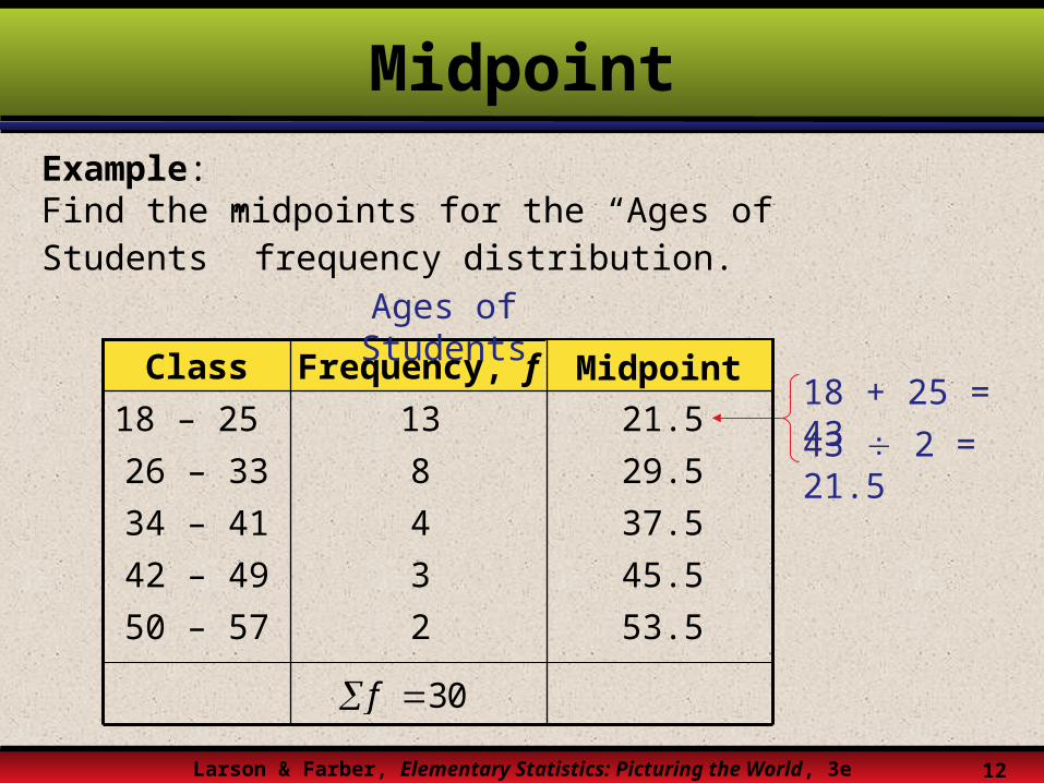
Midpoint

The midpoint of a class is the sum of the lower and upper limits of the class divided by two. The midpoint is sometimes called the class mark.

Midpoint = (Lower class limit) + (Upper class limit) 2

Frequency, fClass Midpoint

41 – 4

Midpoint = 12

4 52

2.5

2.5

Larson & Farber, Elementary Statistics: Picturing the World, 3e 12

MidpointExample:Find the midpoints for the “Ages of Students” frequency distribution.

53.5

45.5

37.5

29.5

21.518 + 25 = 43

43 2 = 21.5

50 – 57

42 – 49

34 – 41

26 – 33

2

3

4

8

1318 – 25

Frequency, fClass

30f

Midpoint

Ages of Students

Larson & Farber, Elementary Statistics: Picturing the World, 3e 13

Relative Frequency

ClassFrequency

, f

Relative Frequenc

y

1 – 4 4

The relative frequency of a class is the portion or percentage of the data that falls in that class. To find the relative frequency of a class, divide the frequency f by the sample size n.

Relative frequency = Class frequencySample size

Relative frequency841

0.222

0.222

fn

18f fn

Larson & Farber, Elementary Statistics: Picturing the World, 3e 14

Relative FrequencyExample:Find the relative frequencies for the “Ages of Students” frequency distribution.

50 – 57 2

3

4

8

13

42 – 49

34 – 41

26 – 33

18 – 25

Frequency, fClass

30f

Relative Frequency

0.067

0.1

0.133

0.267

0.433 fn

1330

0.433

1fn

Portion of students

Larson & Farber, Elementary Statistics: Picturing the World, 3e 15

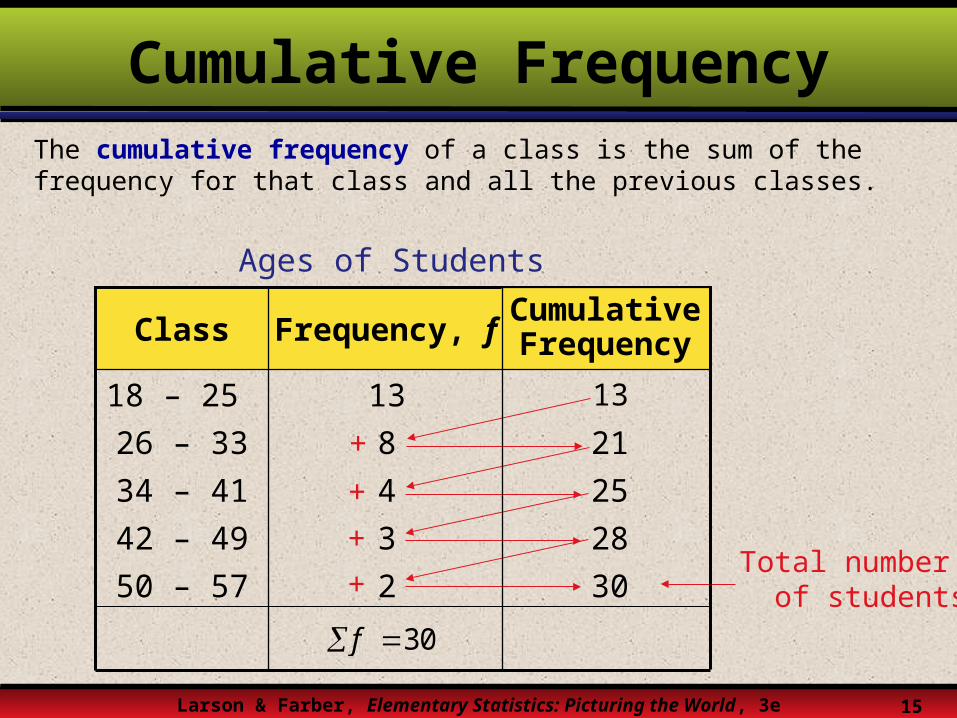
Cumulative FrequencyThe cumulative frequency of a class is the sum of the frequency for that class and all the previous classes.

30

28

25

21

13

Total number of students

+

+++50 – 57 2

3

4

8

13

42 – 49

34 – 41

26 – 33

18 – 25

Frequency, fClass

30f

Cumulative Frequency

Ages of Students

Larson & Farber, Elementary Statistics: Picturing the World, 3e 16

A frequency histogram is a bar graph that represents the frequency distribution of a data set.

Frequency Histogram

1. The horizontal scale is quantitative and measures the data values.

2. The vertical scale measures the frequencies of the classes.

3. Consecutive bars must touch.

Class boundaries are the numbers that separate the classes without forming gaps between them.

The horizontal scale of a histogram can be marked with either the class boundaries or the midpoints.

Larson & Farber, Elementary Statistics: Picturing the World, 3e 17

Class BoundariesExample:Find the class boundaries for the “Ages of Students” frequency distribution.

49.5 57.5

41.5 49.5

33.5 41.5

25.5 33.5

17.5 25.5The distance from the upper limit of the first class to the lower limit of the second class is 1.Half this distance is 0.5.

Class Boundaries

50 – 57 2

3

4

8

13

42 – 49

34 – 41

26 – 33

18 – 25

Frequency, fClass

30f

Ages of Students

Larson & Farber, Elementary Statistics: Picturing the World, 3e 18

Frequency HistogramExample:Draw a frequency histogram for the “Ages of Students” frequency distribution. Use the class boundaries.

23

4

8

13

Broken axis

Ages of Students

10

8

6

4

2

0

Age (in years)

f

12

14

17.5 25.5 33.5 41.5 49.5 57.5

Larson & Farber, Elementary Statistics: Picturing the World, 3e 19

Frequency PolygonA frequency polygon is a line graph that emphasizes the continuous change in frequencies.

Broken axis

Ages of Students

10

8

6

4

2

0

Age (in years)

f

12

14

13.5 21.5 29.5 37.5 45.5 53.5 61.5

Midpoints

Line is extended to the x-axis.

Larson & Farber, Elementary Statistics: Picturing the World, 3e 20

Relative Frequency Histogram

A relative frequency histogram has the same shape and the same horizontal scale as the corresponding frequency histogram.

0.4

0.3

0.2

0.1

0.5

Ages of Students

0

Age (in years)

Rela

tive f

req

uen

cy(p

ort

ion

of

stu

den

ts)

17.5 25.5 33.5 41.5 49.5 57.5

0.433

0.267

0.1330.1

0.067

Larson & Farber, Elementary Statistics: Picturing the World, 3e 21

Cumulative Frequency Graph

A cumulative frequency graph or ogive, is a line graph that displays the cumulative frequency of each class at its upper class boundary.

17.5

Age (in years)

Ages of Students

24

18

12

6

30

0

Cu

mu

lati

ve

freq

uen

cy(p

ort

ion

of

stu

den

ts)

25.5 33.5 41.5 49.5 57.5

The graph ends at the upper boundary of the last class.