design and assessment of fm-mcfs-suited sdm-roadms with

Abstract—In this paper, we focus on the design of different node architectures suitable for Few-Mode Multi-Core Fibers (FM-MCFs) based networks. Both dimensions, core and mode, open different possible ways to group spatial channels depending on the physical impairments of the Space-Division Multiplexed (SDM) optical fibers. Moreover, the channel switching across a group of cores/modes at once and the end-to-end routing are not only mandatory aspects for certain spatial channels, but also recommendable in order to reduce the node complexity/cost. Thus, we propose various SDM-capable node architectures based on versatile and homogeneous spatial group configurations. Then, a unified physical-layer-aware Quality of Transmission (QoT) estimator is formulated to not only evaluate these node architectures in a simulation tool, but also validate them in a real experimental environment using a stateful Path Computation Element (PCE) as a central controller. The obtained results disclose that the cost-efficient node design parameter, namely, the size of the spatial group 𝑮 , depends on both the network and traffic profile size. Specifically, for a national optical backbone network equipped with a homogeneous and hexagonally arranged 6-weakly-coupled modes and 7-weakly-coupled cores fibers, 𝑮 equals 6, while for a continental backbone network, 𝑮 can raise up to 14. In any case, we demonstrate that the cost-benefit tradeoff in node design must be analyzed in detail in order to meet the huge traffic volumes of the next years.

Index Terms—SDM, FM-MCFs, QoT Estimator, ROADMs, Network Design, Resource Allocation.

NOMENCLATURE

A/D add/drop

ASE amplified spontaneous emission

AoD architecture on demand

BBP bandwidth blocking probability

BER bit error rate

BV-OXC bandwidth variable optical cross connect

BVT bandwidth variable transponder

R. Rumipamba-Zambrano is with the Corporación Nacional de Telecomunicaciones CNT E.P., 170518 Quito, Ecuador; Coordinación de Investigación e Innovación, ABREC, 170528 Quito, Ecuador, and with the Institute for Applied Sustainability Research, Quito, Ecuador (e-mail: [email protected]) R. Muñoz and R. Casellas are with the Centre Tecnològic de Telecomunicacions de Catalunya, Barcelona 08860, Spain (e-mail: [email protected]; [email protected]). J. Perelló and S. Spadaro are with the Advanced Broadband Communications Center (CCABA), Universitat Politècnica de Catalunya (UPC) – Barcelona

CAPEX capital expenditures

CD chromatic dispersion

D nodal degree

DMGD differential modal group delay

DP dual-polarization

DSP digital signal processing

DT12 12-node deutsche telekom optical network

EDFA erbium-doped fiber amplifier

EON elastic optical network

EROs explicit route objects

FF first-fit

FEC forward error correction

FJoS fractional joint switching

FMF few-mode fiber

FM-MCFs few-mode multi-core fibers

FM-SSS few-mode-based SSS

FS frequency slot

G group size

GB guard-band

GLC group lane change

GN Gaussian-noise

GVD group velocity dispersion

HT holding time

I number of connected SDM fibers in an SDM-ROADM

IAT inter-arrival time

ICXT inter-core crosstalk

ICS inter-core skew

IMXT inter-mode crosstalk

InS with LC independent switching with lane change support

Tech, 08034 Barcelona, Spain (e-mail: [email protected]; [email protected] ). Abdulaziz E. Elfiqi is with School of Engineering, The University of Tokyo, 7-3-1 Hongo, Bunkyo-ku, Tokyo, Japan, and with the Electronics and Electrical Communications Engineering Department, Faculty of Electronic Engineering, Menoufia University, Menouf 32952, Egypt (e-mail: [email protected]).

Copyright (c) 2020 IEEE.

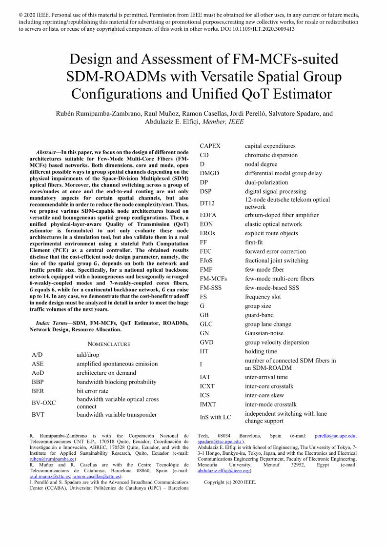
Rubén Rumipamba-Zambrano, Raul Muñoz, Ramon Casellas, Jordi Perelló, Salvatore Spadaro, and Abdulaziz E. Elfiqi, Member, IEEE

Design and Assessment of FM-MCFs-suited SDM-ROADMs with Versatile Spatial Group Configurations and Unified QoT Estimator1

© 2020 IEEE. Personal use of this material is permitted. Permission from IEEE must be obtained for all other uses, in any current or future media, including reprinting/republishing this material for advertising or promotional purposes,creating new collective works, for resale or redistribution to servers or lists, or reuse of any copyrighted component of this work in other works. DOI 10.1109/JLT.2020.3009413

InS w/o LC independent switching without lane change support

I2 internet 2

J core count

JoS joint switching

K mode count

L offered load

LC lane change

LP linear polarized

MCFs multi-core fibers

MDL mode-dependent loss

MEM micro-electro-mechanical

MIMO multiple-input multiple-output

MMFs multi-mode fibers

MPLS multi-protocol label switching

MUX/DEMUX multiplexer/demultiplexer

NLI non-linear interference

NLSE nonlinear Schrödinger equation

ODLs optical delay lines

OPEX operational expenditures

OSNR optical signal-to-noise-ratio

PCE path computation element

PCECC PCE central controller

PCEP PCE protocol

PCReq path computation request

PM polarization multiplexing

QoT quality of transmission

RA resource allocation

ROADM reconfigurable optical add/drop multiplexer

RMCMSA route, modulation format, core, mode and spectrum assignment

RMCSA route, modulation format, core and spectrum assignment

RMMSA route, modulation format, mode and spectrum assignment

RMSA route, modulation format and spectrum assignment

RSA route, spectrum assignment

Rx receiver

S spatial multiplicity

SCh super-channel

SCh BVT super-channel bandwidth-variable transponder

SDM space division multiplexing

SDM-EON SDM-based elastic optical network

SDM-ROADM SDM-capable roadm

SDM-SSS SDM-based SSS

SDN software defined networks

SE spectral efficiency

SEROs secondary explicit route objects

SLC subgroup lane change

SMF single-mode fiber

SMFB single-mode fiber bundle

SNR signal-to-noise-ratio

SP shortest path

Spa-SCh spatial super-channel

Spe-SCh spectral super-channel

SSS spectrum selective switch

TED traffic engineering database

TP traffic profile

TR transmission reach

WDM wavelength division multiplexing

XT crosstalk

I. INTRODUCTION

HE emerging telecom services in the 5G era, such as ultra-high-definition video streaming, cloud computing,

connected car, virtual/augmented reality, etc., have enormously increased the traffic volume that has to be supported by all network regions. According to the literature, network traffic multiplies by 10-fold every 4 years [1]. For this reason, optical technologies have continuously evolved in the last years in order to keep pace with this exponential traffic growth. For example, in the early 90’s, Wavelength Division Multiplexing (WDM) technology was proposed, using a fixed frequency grid. Some years later, a flexible frequency grid was introduced, arising the concepts of Flex-Grid WDM and Elastic Optical Networks (EON) [2]. EONs aimed at increasing the Spectral Efficiency (𝑆𝐸) of Single-Mode Fibers (SMFs) by allocating a variable-sized Frequency Slot (FS). Furthermore, a group of optical signals occupying a set of FSs can form optical Super-Channels (SChs). Nevertheless, SMFs’ capacity will be unable to cope with the enormous bandwidth requirements giving rise to unavoidable collapse [3], [4] when the so-called non-linear Shannon’s limit is reached. A promising alternative to tackle this issue is the Space Division Multiplexing (SDM) technology, which proposes to enable parallel optical paths in order to surpass the 100 Tb/s capacity of SMF-based systems. However, besides parallelization, integration and sharing of system components is necessary [1], [4]–[6] in order to reduce the cost and energy per bit regarding today’s SMF systems. Both Flex-Grid WDM and SDM technologies are orthogonal in principle, but their combination [7]–[9] in the so-called SDM-EON networks emerges as an attractive solution to scale up the network capacity even more. Furthermore, a gradual migration from EON towards SDM-EON is required to be carried out as the demand capacity grows up [10].

T

Nowadays, there are mainly four transmission media candidates to realize SDM: i) a bundle of SMFs (SMFB) within the same fiber ribbon cable, ii) a single mode transmitted in several cores within the same fiber cladding, namely, Multi-Core Fibers (MCFs), iii) a transmission of multiple or some guided modes within the same fiber core, namely, Multi-Mode Fibers (MMFs) or Few-Mode Fibers (FMFs), respectively, and iv) a combination of FMFs and MCFs, i.e., few modes are transmitted in various cores within the same fiber-cladding (FM-MCFs). The latter three SDM fiber types suffer from different impairments, such as Differential Mode Group Delay (DMGD) and both linear and/or nonlinear crosstalk (XT) between modes and/or cores. The XT level limits the application scope to short- or long-reach communications [11]. Moreover, transparent communication, i.e., without regeneration, is only possible until the XT threshold is attained, unless Multiple-Input Multiple-Output (MIMO) is applied [12]–[14]. Various SDM fiber layouts including homogeneous and heterogeneous MCFs [15], [16] with ultra-low XT levels have been demonstrated for long-haul communications [17], [18], even fibers with high spatial channel count [19]. Heterogeneous MCFs enables Dense-SDM and may lower the linear XT [16]. However, the application of MIMO-DSP can become prohibited in long-haul transmission since they exhibit higher DMGD than homogeneous MCFs increasing the memory length of such MIMO systems [12].

The SDM fiber candidates also determine the options for optical channel switching at the SDM-capable Reconfigurable Optical Add/Drop Multiplexers (SDM-ROADMs). Some node architectures have been proposed for SDM, based on hard-wired internal connections [20], [21] and Architecture on Demand (i.e., customized internal connections according to traffic needs) [22]. Specifically, the so-called Independent switching (InS), Fractional Joint Switching (FJoS) and Joint Switching (JoS) options are suitable for different SDM fibers depending on the XT level [23]. Thus, InS can be only applied to uncoupled SDM fibers, FJoS to uncoupled or weakly coupled, while JoS to any kind of SDM fiber. Until now, to the best of our knowledge, these node architectures have been mainly applied to the first three types of SDM fibers mentioned before (i.e., SMFBs, MCFs, FMFs), while only [24] considers particular node architectures for a 3-mode 7-core SDM fiber.

In the case of FM-MCFs, a suitable node architecture to be applied is FJoS, where the group switching size (𝐺) can be equal to the mode count (𝐾 ) transmitted by each core 𝑗 . However, weak-coupling regime, where both intermodal (IM) and inter-core (IC) linear crosstalk (XT) are very small compared to the linear polarization coupling and other interferences (Amplified Spontaneous Emission ASE noise and nonlinear interference) [25], enables different feasible 𝐺 configurations to be tested, depending on the spatial multiplicity (𝑆 𝐽 ∙ 𝐾 , being 𝐽 the core count within a fiber cladding). The fact is that different mode groups inside each core of the weakly-coupled modes and cores FM-MCFs (henceforth referred to as weakly-coupled FM-MCFs solely) can be treated as independent transmission streams [26]–[28]. Nowadays, the applicability of this approach has been

demonstrated for short-reach transmission (e.g., access, metro, intra-data center, etc.), where DSP complexity is relaxed by applying MIMO-free or partial MIMO [26], [29]–[31]. Nevertheless, some initial efforts and investigations have been also carried out in long-haul transmission [32]–[34].

Ongoing researches are focused on solving various challenges such as: suppression of DMGD within every mode group, suppression of IMXT and mode-dependent loss (MDL) at butt coupling, etc. [32] in order to realize long-haul weakly-coupled FM-MCF transmission. These challenges can be tackled by applying a combination of different techniques and design parameters, namely, refractive-index profiles, effective index difference between modes ( ∆ ), fiber geometry, splicing technologies, photonic lanterns or silicon-photonic-based multiplexers, ring-core FM erbium-doped fiber amplifiers, free-space optics type gain equalizer, DMGD compensation, etc. [27], [33]–[36].

Unlike [24], where only one case of FJoS (unique 𝐺) for a particular FM-MCF structure is evaluated, this study considers these expected homogeneous weakly-coupled FM-MCFs for long-haul transmission to study different channel switching schemes including the physical-layer impairments analysis in FM-MCFs transmission by considering the linear and nonlinear effects in a unified developed QoT estimator. Then, we design their corresponding specialized node architectures and evaluate them for different optical backbone networks and under different traffic profiles. Furthermore, different channel switching schemes in node architectures lead to propose various resource allocation mechanisms for weakly-coupled-FM-MCFs-based networks.

The rest of this paper is organized as follows. Section II presents the FM-MCFs-based networks, where different SDM-ROADM architectures are discussed. In Section III, the QoT model is proposed and explored. The algorithms for resource allocation and network provisioning are described in Section IV. Section V presents the numerical evaluation in three subsections. Subsection V.A describes the scenario details and assumptions. The performance evaluation of the different proposed SDM-ROADMs architectures is presented in subsection V.B, while the experimental validation is shown in subsection V.C. Finally, Section VI draws up the main conclusions and envisions future work.

II. FM-MCFS-BASED SDM NETWORKS

A typical SDM network (Fig. 1) is composed of SDM-ROADMs linked by SDM fibers, e.g., weakly-coupled FM-MCFs. Other network elements are spectral/spatial SCh Bandwidth-Variable Transponders (BVTs) [37] connected to the Add/Drop (A/D) modules of the SDM-ROADMs, as well as amplifiers in between nodes (not shown in Fig. 1). Note that regenerators are not considered in transparent optical networks, as the one shown in Fig. 1. Here, an SDM link deploys several parallel optical-paths. For instance, if a 6-modes 7-cores SDM fiber is considered, the total number of parallel optical-paths is given by the spatial multiplicity, i.e., 𝑆 𝐽 ∙ 𝐾 7 ∙ 6 42. One connection (or lightpath) is established between two SDM-

ROADMs that, in this case, can be composed by a group of optical paths carrying a common wavelength (color).

In FM-MCFs, we have to deal with XT between cores and propagated modes. However, if the core pitch and diameter are large and short enough [38], respectively, the so-called weakly-coupled MCFs allows transparent long-haul communications. Meanwhile, if coherent detection is used, any mode coupling can be compensated fully [39], [40] by applying full MIMO at the receiver side (Rx). In weak-couple regime (considered in this work), the IMXT between spatial modes of different groups can be neglected and these modes are known as non-degenerate, while the spatial modes of the same group are strongly coupled and called as degenerate modes because they experiment similar propagation constants [27], [41].

Fig. 1. Basic SDM network elements.

If such strongly-coupled degenerate modes transmitted per core are discriminated, then the MIMO-DSP complexity and power consumption can be reduced by processing each mode group separately [26], [39]. In other words, low-complexity partial MIMO can be applied for each mode group comprising degenerate modes of the same high-order Linearly Polarized (LP) mode (e.g., LP11a and LP11b is a two-fold degeneracy mode group). To illustrate this, in Fig. 2, we represent a full 12 12 MIMO for 4-LP modes in strong-coupling regime versus a 2 ∙ ( 4 4 ) plus 2 ∙ (2 2) MIMO in weak-coupling regime (considered in this work) in order to decouple linear impairments. Here, we can observe MIMO equalization for 4 independent mode subgroups, instead of applying it for one general group of 6 spatial modes.

Fig. 2. (a) Full and (b) partial MIMO equalization for strong-coupling and weak-coupling regime, respectively.

A. SDM-ROADM Architectures for FM-MCFs

Regular ROADMs (for SMF) are in charge of automatically adding, dropping or bypassing (transparent switching) lightpaths in Flex-Grid WDM networks. The design of these ROADMs includes Spectrum Selective Switch (SSS) devices, which are able to switch any FS from any of its input ports to any of its output ports [42]. Extending this node architecture to SDM-EON networks, as shown in Fig. 3, SDM-SSSs have been defined [20], [43] to manage 𝑀 𝑁 instead of 1 𝑁 ports. These SDM-SSSs are especially useful for spatial group switching [23], where one spectrum portion is switched across 𝑀 𝑆 spatial channels at once. This strategy represents the real spirit of SDM networks where integration and sharing of system components are expected; otherwise, the architecture would become equivalent to a parallel arrangement of regular ROADMs with 1 𝑁 SSSs, as the design of the so-called space-continuity-constrained SDM-ROADMs (cf. Fig. 1(c) [44]). Indeed, these kind of nodes fulfilling the space continuity constraint are known in the literature as InS without Lane Change (LC) support [20], [45]. The LC support is defined as the ability to realize spatial conversion that for SMFBs and MCFs implies to switch the channel transmission from one fiber/core to another, respectively. In contrast, for FMFs this capacity requires mode conversion [46], while for FM-MCFs both types of spatial conversion are possible: mode conversion and/or core switching.

On the other hand, an SDM-ROADM must include an SDM MUX/DEMUX, which combines/separates spatial channels, either through FAN-IN/FAN-OUT or MODE MUX/DEMUX for cores or modes, respectively, as shown in Fig. 3. Specifically for FMFs or FM-MCFs, there are two SSS adaptation options for JoS/FJoS operation: spatial diversity and multi-mode beams [47]–[49]. On one side, spatial diversity [Fig. 3(a)] is the straightforward solution, requiring to separate all spatial channels in single-mode inputs, because the reconfiguration is based on 1 𝑁 SSSs for SMFs by exciting simultaneously various input ports with micro-electro-mechanical (MEMs) micromirrors [50]. In this design, for example, we can appreciate the four subgroups formed by LP , LP and LP , LP fundamental and high-order LP modes, respectively, distinguished by colored solid lines (see also Table I). On the other side, the multi-mode beams alternative [Fig. 3(b)], directly accomplishes 1 𝑁 FM-SSSs by replacing an SMF collimator array with an FMF collimator one. These FM-SSSs allow having an identical switching approach and design as SMF-based WDM systems, while they show wider channel transitions (as mode count increases) requiring larger spectral Guard-bands [43]. For this reason, spatial-diversity-based SDM-SSSs are preferred in the SDM-ROADM design realizing JoS/FJoS operation. In Fig. 3(b), we can appreciate that MODE MUX/DEMUX is not necessary since FM-SSSs are able to manage multi-mode connections (up to 𝐾 spatial modes per physical port). Hereinafter, LP will refer to a specific spatial mode of FM-MCFs layout (i.e., when we know what LP mode is transmitted), while 𝑚 will refer to a generic spatial mode of FM-MCFs layout supporting 𝐾 spatial modes. An

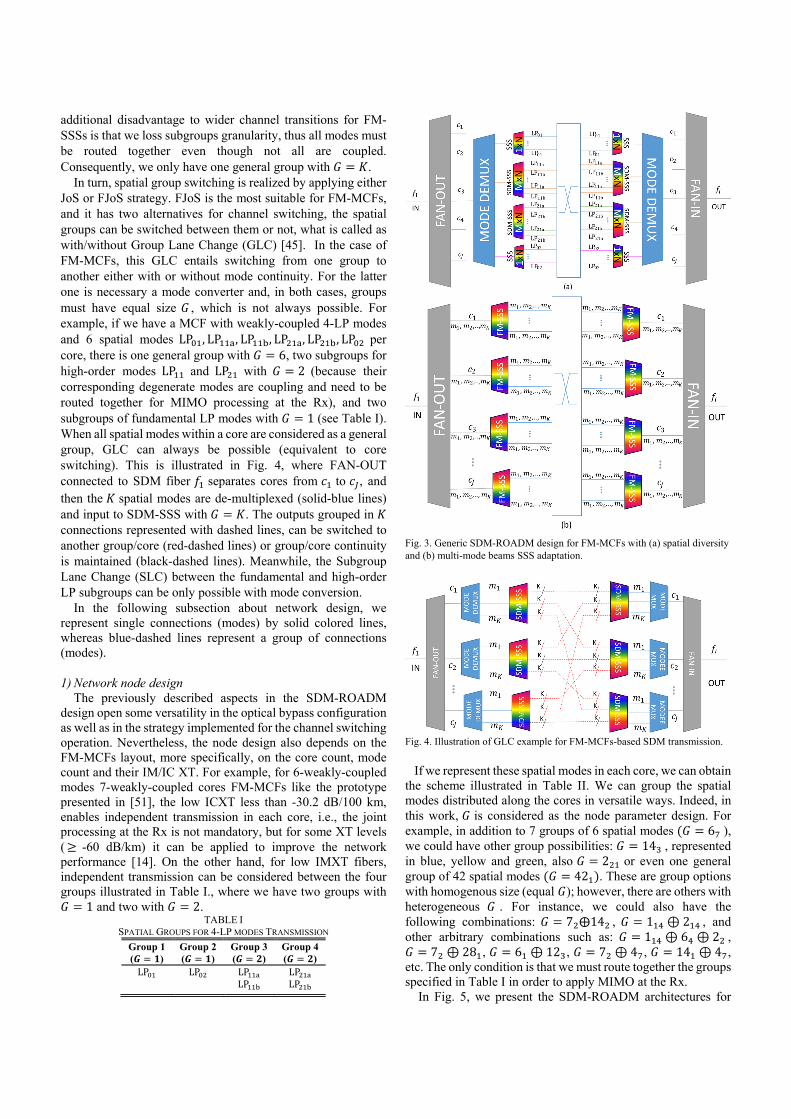
additional disadvantage to wider channel transitions for FM-SSSs is that we loss subgroups granularity, thus all modes must be routed together even though not all are coupled. Consequently, we only have one general group with 𝐺 𝐾.

In turn, spatial group switching is realized by applying either JoS or FJoS strategy. FJoS is the most suitable for FM-MCFs, and it has two alternatives for channel switching, the spatial groups can be switched between them or not, what is called as with/without Group Lane Change (GLC) [45]. In the case of FM-MCFs, this GLC entails switching from one group to another either with or without mode continuity. For the latter one is necessary a mode converter and, in both cases, groups must have equal size 𝐺 , which is not always possible. For example, if we have a MCF with weakly-coupled 4-LP modes and 6 spatial modes LP , LP , LP , LP , LP , LP per core, there is one general group with 𝐺 6, two subgroups for high-order modes LP and LP with 𝐺 2 (because their corresponding degenerate modes are coupling and need to be routed together for MIMO processing at the Rx), and two subgroups of fundamental LP modes with 𝐺 1 (see Table I). When all spatial modes within a core are considered as a general group, GLC can always be possible (equivalent to core switching). This is illustrated in Fig. 4, where FAN-OUT connected to SDM fiber 𝑓 separates cores from 𝑐 to 𝑐 , and then the 𝐾 spatial modes are de-multiplexed (solid-blue lines) and input to SDM-SSS with 𝐺 𝐾. The outputs grouped in 𝐾 connections represented with dashed lines, can be switched to another group/core (red-dashed lines) or group/core continuity is maintained (black-dashed lines). Meanwhile, the Subgroup Lane Change (SLC) between the fundamental and high-order LP subgroups can be only possible with mode conversion.

In the following subsection about network design, we represent single connections (modes) by solid colored lines, whereas blue-dashed lines represent a group of connections (modes).

1) Network node design The previously described aspects in the SDM-ROADM

design open some versatility in the optical bypass configuration as well as in the strategy implemented for the channel switching operation. Nevertheless, the node design also depends on the FM-MCFs layout, more specifically, on the core count, mode count and their IM/IC XT. For example, for 6-weakly-coupled modes 7-weakly-coupled cores FM-MCFs like the prototype presented in [51], the low ICXT less than -30.2 dB/100 km, enables independent transmission in each core, i.e., the joint processing at the Rx is not mandatory, but for some XT levels ( -60 dB/km) it can be applied to improve the network performance [14]. On the other hand, for low IMXT fibers, independent transmission can be considered between the four groups illustrated in Table I., where we have two groups with 𝐺 1 and two with 𝐺 2.

TABLE I SPATIAL GROUPS FOR 4-LP MODES TRANSMISSION

Group 1 (𝑮 𝟏)

Group 2 (𝑮 𝟏)

Group 3 (𝑮 𝟐)

Group 4 (𝑮 𝟐)

LP LP

LP LP

LP LP

Fig. 3. Generic SDM-ROADM design for FM-MCFs with (a) spatial diversity and (b) multi-mode beams SSS adaptation.

Fig. 4. Illustration of GLC example for FM-MCFs-based SDM transmission.

If we represent these spatial modes in each core, we can obtain the scheme illustrated in Table II. We can group the spatial modes distributed along the cores in versatile ways. Indeed, in this work, 𝐺 is considered as the node parameter design. For example, in addition to 7 groups of 6 spatial modes 𝐺 6 ), we could have other group possibilities: 𝐺 14 , represented in blue, yellow and green, also 𝐺 2 or even one general group of 42 spatial modes 𝐺 42 . These are group options with homogenous size (equal 𝐺); however, there are others with heterogeneous 𝐺 . For instance, we could also have the following combinations: 𝐺 7 ⨁14 , 𝐺 1 ⊕ 2 , and other arbitrary combinations such as: 𝐺 1 ⊕ 6 ⊕ 2 , 𝐺 7 ⊕ 28 , 𝐺 6 ⊕ 12 , 𝐺 7 ⊕ 4 , 𝐺 14 ⊕ 4 , etc. The only condition is that we must route together the groups specified in Table I in order to apply MIMO at the Rx.

In Fig. 5, we present the SDM-ROADM architectures for

FM-MCFs with homogeneous 𝐺 considering spatial-diversity-based SDM-SSSs, given the previously described advantages that they offer. Moreover, note that with the design based on multi-mode beams, group switching configurations 𝐺 14 , 𝐺 2 would not be affordable because this re-arrangement of the spatial groups is configured after de-multiplexing the spatial modes, while 𝐺 42 should be supported by not yet demonstrated 𝑀 𝑁 FM-SSSs. From Fig. 5 to Fig. 7 can be considered as general schemes for whatever FM-MCFs layout, while Fig. 8 and Fig. 9 are particular cases for MCF layouts with 𝐾 6 . For JoS SDM-ROADM, represented in Fig. 5, depending on the spatial multiplicity, the design can nowadays be unaffordable, owing to the current commercial SSS sizes; however, it is worth to be considered for benchmark purposes. Among the homogeneous groups for 6-mode 7-core SDM fiber, unlike 𝐺 14 , 𝐺 6 allows GLC without mode conversion, whereas for 𝐺 2 , SLC can be done by applying core switching and/or mode conversion. For the sake of simplicity, we show and evaluate in Section IV, node architectures where GLC/SLC does not imply mode conversion; otherwise, node architectures with group/subgroup continuity are only considered.

TABLE II 6-MODE REPRESENTATION INSIDE 7-CORES AND GROUP OPTIONS

core mode 1 2 3 4 5 6 7

1 LPo1 LPo1 LPo1 LPo1 LPo1 LPo1 LPo1

2 LPo2 LPo2 LPo2 LPo2 LPo2 LPo2 LPo2

3 LP11a LP11a LP11a LP11a LP11a LP11a LP11a

4 LP11b LP11b LP11b LP11b LP11b LP11b LP11b

5 LP21a LP21a LP21a LP21a LP21a LP21a LP21a

6 LP21b LP21b LP21b LP21b LP21b LP21b LP21b

For these SDM-ROADMs, we show a design for 𝐼-connected SDM fibers, i.e., nodal degree (𝐷 𝐼), each fiber 𝑓 has 𝐽 cores and, in its turn, each core transmits 𝐾 spatial modes. Cores 𝑐 ,…,𝑐 and modes 𝑚 ,…,𝑚 are combined/separated by an SDM MUX/DEMUX. Each SDM-SSS must include one group of ports for A/D operation, whose connection is represented by gray-dotted lines, therefore, the SDM-SSS size can be generalized as 𝐺 𝐼 ∙ 𝐺 when GLC/SLC is not supported. Moreover, the required number of SDM-SSSs per node is 2 ∙

𝑔𝑟𝑜𝑢𝑝_𝑐𝑜𝑢𝑛𝑡 ∙ 𝐼, where 𝑔𝑟𝑜𝑢𝑝_𝑐𝑜𝑢𝑛𝑡 ∙

. Traffic

in each node is injected/extracted by Spatial Super-Channel (Spa-SCh) BVTs connected to A/D module.

For JoS, shown in Fig. 5, 𝐺 𝐽 ∙ 𝐾 and group continuity is implicit. Therefore, the SDM-SSS size is equal to 𝐽 ∙ 𝐾 𝐼 ∙𝐽 ∙ 𝐾 . Figure 6 and Fig. 7 represent FJoS with 𝐺 𝐾 with

and without GLC, respectively. Consequently, the size of SDM-SSSs for FJoS ( 𝐺 𝐾 ) with GLC is 𝐾 𝐼 ∙ 𝐽 ∙ 𝐾 and for the one without GLC is 𝐾 𝐼 ∙ 𝐾. On the other hand, Fig. 8 shows the SDM-ROADM architecture for FJoS with 𝐺 2 ∙ 𝐽 without SLC. The LP modes of each core are grouped in an SDM-SSS with 2 ∙ 𝐽 𝐼 ∙ 2 ∙ 𝐽 size. Finally, Fig. 9 shows the

node architecture for FJoS with 𝐺 2 ∙ , having 3 groups formed by LP , LP ; LP , LP and LP , LP . The SLC is not considered, i.e., core and mode continuity constraints are fulfilled, therefore the SDM-SSS size is 2 𝐼 ∙ 2. Table III. Summarizes the SDM-SSS parameters for different SDM-ROADM presented before.

Fig. 5. SDM-ROADM architecture for JoS, 𝐺 𝐽 ∙ 𝐾 , and 𝐷 2.

Fig. 6. SDM-ROADM architecture for FJoS with 𝐺 𝐾 and GLC, 𝐷 2

Fig. 7. SDM-ROADM architecture for FJoS without GLC and with 𝐺 𝐾 , 𝐷 2.

Fig. 8. SDM-ROADM architecture for FJoS with 2 ∙ 𝐽 , and 𝐷 2.

Fig. 9. SDM-ROADM architecture for FJoS with 𝐺 2 ∙ , 𝐷 2 (only drop connections are shown for simplicity).

TABLE III SDM-SSS PARAMETERS FOR EACH SDM-ROADM

SDM-ROADM SDM-SSS size SDM-SSS count JoS (𝐺 𝐽 ∙ 𝐾) 𝐽 ∙ 𝐾 𝐼 ∙ 𝐽 ∙ 𝐾

2 ∙ 𝑔𝑟𝑜𝑢𝑝_𝑐𝑜𝑢𝑛𝑡 ∙ 𝐼 FJoS (𝐺 𝐾, w/ GLC) 𝐾 𝐼 ∙ 𝐽 ∙ 𝐾 FJoS (𝐺 𝐾, w/o GLC) 𝐾 𝐼 ∙ 𝐾 FJoS (𝐺 2 ∙ 𝐽 , w/o SLC) 2 ∙ 𝐽 𝐼 ∙ 2 ∙ 𝐽 FJoS (𝐺 2 ∙ , w/o SLC) 2 𝐼 ∙ 2

III. FM-MCFS-BASED QOT ESTIMATOR

A. QoT Model

In this subsection, we develop a unified expression of the end-to-end QoT for weakly-coupled-FM-MCFs-based networks. The signal propagation of dual-polarized (DP) transmission in dispersive- nonlinear fiber is represented by the nonlinear Schrödinger equation (NLSE) [25], [41], [52]. For FM-MCFs, we can formulate NLSE for 𝐾-multi-modes inside 𝐽-multi-cores fiber as follows:

𝜕𝑨

𝜕𝑧𝛼2𝑨𝒗𝒖 jβ𝑨 𝑄 𝑨

j43γ 𝜁

23

𝑨 𝑨∗ 𝑨

j ∑ 𝑤 𝑨 𝑨 𝑨∗ 2 𝑨 𝑨 𝑨 ,(1)

where 𝑨 is the vector field envelope for mode (𝑣 within core ( 𝑢 ) expressed for dual-polarization as 𝐴 𝐴 . T, H denotes to the transpose and Hermitian-transpose of a vector, and 𝛿 is the Kronecker delta function. 𝛼 and β are the attenuation coefficient and average group velocity dispersion (GVD) parameter of the propagating modes, respectively, and γ is the nonlinear coefficient. 𝑄 is the linear-coupling XT

between different signal (mode 𝑘 in core 𝑗 with mode 𝑣 in core u), 𝜁 represent the intra- and inter-modal nonlinear tensors, and 𝑤 are the inter-core nonlinear tensors. The

above equation contains different FM-MCFs impairments: linear DMGD between different modes (2nd term), linear inter-core XT (3rd), nonlinear inter- and intra-modal XT (4th), and nonlinear intra-cores XT (5th).

In order to obtain a unified analytical model for QoT based on FM-MCFs, we follow a similar procedure as in [52], [53] and adopt the well-known Gaussian-Noise (GN) model for long-haul FM-MCFs transmission. Based on a rigorous mathematical analysis, we obtain the nonlinear interference XT as:

XT ,

𝑃 ∑ sinh 𝜓

sinh 𝜓 ∑

sinh 𝜓 , (2)

where,

𝜓√34𝜋𝐿 , 𝑁 𝐵

√34 𝜋 𝛽 𝑁 𝐵 ∆𝛽

1 ∑ 𝑄,

𝜓 ,

∑,

and 𝑃 is the channel power, 𝐵 is the noise bandwidth, ∆𝛽 is the DMGD between different co-propagated modes inside the same core. 𝑁 is the number of co-propagated channels, 𝐵 is the WDM channel spacing, 𝐿 , 1 2α and 𝐿 1 𝑒 2𝛼𝐿 2𝛼 are the asymptotic-effective and effective length, respectively, for a span length 𝐿𝑠. Finally, the Transmission Reach (TR, i.e., the maximum achievable distance), as a QoT metric, pending to specific forward error correction (FEC) limit of BER can be obtained as:

TR 𝐿 SNR , (3)

where ⌊. ⌋ is the floor-integer of a value, 𝐿 is the span length and SNR is the correspondence Signal-to-Noise ratio to

the FEC-BER limit. P denotes the EDFA noise per node and

XT is the MUX/DEMUX imperfect-interference. XT

is the linear ICXT and can be expressed as XT 𝐽

1 𝐿 Q 𝑃 for the center-core in homogeneous and

hexagonally arranged J-weakly-coupled cores FM-MCFs, where 𝑅 is the bending radius and Λ is the pitch distance [54].

One important aspect that should be considered is the propagation delay difference between cores, sometimes referred in the literature to as inter-core skew (ICS) [12]. If such ICS is not properly compensated in the fiber link, the memory length of the MIMO systems increases linearly with the transmission distance limiting the TR. However, a combination of Optical Delay Lines (ODLs) [12] and residual ICS compensation at SDM-ROAMs can prevent large memory length requirements of such partial MIMO systems considered in this work.

B. QoT Estimations

Considering the analytical model described above, in this subsection we present the results of the QoT estimations by taking into account some parameters. Table IV and V show the summary of the main physical parameters for a homogeneous and hexagonally arranged 6-modes 7-cores FM-MCF as well as for transmission, respectively, taken from [41], [52]. Moreover, the XT assumed is about -52 dB/km (2-dB compensation for

the worst ICXT value reported in [51] for long edge of the C-band), while a perfect MUX/DEMUX with zero interference is considered.

TABLE IV MAIN PHYSICAL PARAMETERS FOR A HOMOGENEOUS 6-WEAKLY-COUPLED

MODES AND 7-WEAKLY-COUPLED CORES FM-MCF

Parameter Symbol Value Nonlinear coefficient 𝛾 1.4 W−1km−1

Chromatic Dispersion CD 21.5 ps/km∙nm

attenuation 𝛼 0.22 dB/km

TABLE V MAIN PHYSICAL PARAMETERS FOR TRANSMISSION

Parameter Symbol Value ASE noise 𝐏𝐀𝐒𝐄 -30 dBm

Bit Error Rate BER 10 Forward Error Correction FEC 20%

Span length 𝑳𝒔 80 km

Channel spacing 𝐁𝒄𝒉 41 GHz

Number of channels 𝐍𝒄𝒉 10

Symbol rate 𝑹𝒔 32 GBaud

Wavelength 𝝀 1550 nm

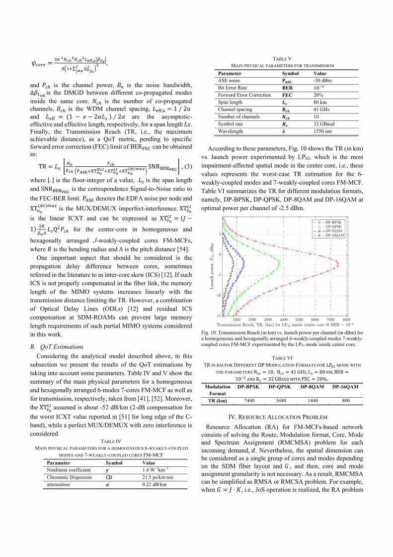
According to these parameters, Fig. 10 shows the TR (in km)

vs. launch power experimented by LP02, which is the most impairment-affected spatial mode in the center core, i.e., these values represents the worst-case TR estimation for the 6-weakly-coupled modes and 7-weakly-coupled cores FM-MCF. Table VI summarizes the TR for different modulation formats, namely, DP-BPSK, DP-QPSK, DP-8QAM and DP-16QAM at optimal power per channel of -2.5 dBm.

Fig. 10. Transmission Reach (in km) vs. launch power per channel (in dBm) for a homogeneous and hexagonally arranged 6-weakly-coupled modes 7-weakly-coupled cores FM-MCF experimented by the LP02 mode inside center core.

TABLE VI TR IN KM FOR DIFFERENT DP MODULATION FORMATS FOR LP MODE WITH

THE PARAMETERS N 10, B 41 GHZ, L 80 KM, BER10 AND R 32 GBAUD WITH FEC 20%.

Modulation Format

DP-BPSK DP-QPSK DP-8QAM DP-16QAM

TR (km) 7440 3680 1440 800

IV. RESOURCE ALLOCATION PROBLEM

Resource Allocation (RA) for FM-MCFs-based network consists of solving the Route, Modulation format, Core, Mode and Spectrum Assignment (RMCMSA) problem for each incoming demand, 𝑑. Nevertheless, the spatial dimension can be considered as a single group of cores and modes depending on the SDM fiber layout and 𝐺 , and then, core and mode assignment granularity is not necessary. As a result, RMCMSA can be simplified as RMSA or RMCSA problem. For example, when 𝐺 𝐽 ∙ 𝐾, i.e., JoS operation is realized, the RA problem

is equivalent to RMSA since the demand capacity, 𝑟 , is equally split into 𝐽 ∙ 𝐾 spatial channels. In contrast, if 𝑟 is divided into 𝐾 spatial modes, the RMCSA problem arises, and then, one core index has to be assigned to each demand either fulfilling the core continuity or not. Meanwhile, other 𝐺 sizes may entail assigning one core index and/or LP mode(s).

Consequently, as some dimension ( 𝐽 and/or 𝐾 ) can be suppressed during the RA process depending on the considered 𝐺, some equivalent node architectures appear from the channel routing point of view. For example, JoS node architecture for routing purposes is equivalent to SMF-based ROADM, while the RA considering FJoS w/o GLC architecture is equivalent to carry it out for InS w/o LC one, with the difference that 𝑟 is divided into 𝑛 spatial channels, e.g., into 6 spatial modes represented in the FM-MCF of Table II. In other words, the Spa-SCh spans 6 spatial modes, but in practice, it is equivalent to allocate a Spectral Super-Channel (Spe-SCh) over one single spatial group. Furthermore, a demand 𝑑 can require to be allocated onto 𝑛 𝐺 spatial channels, occupying 𝑛 spatial

groups 𝑛 , therefore, this situation is equivalent to

allocate a Spa-SCh over two or more spatial groups. Note that 𝑛 would be the number of spatial channels generated by a Spa-SCh BVT. Table VII summarizes the equivalent RA problems to be addressed for the node architectures detailed in Table III. Here, we can see that the architecture counterpart for three cases is the same InS w/o LC; however, the RA problem to be solved is slightly different, namely, RMCSA, RMMSA and RMCMSA. In general, the required spectral resources, i.e., the required number of FSs (𝑛 ) for a demand, 𝑑, spanning 𝑛 ∙ 𝐺 spatial channels are given by:

𝑛∙ ∙

, (4)

where 𝑆𝐸 is the spectral efficiency, 𝐺𝐵 and 𝑊 account for Guard-band and FS width, respectively, both in GHz.

TABLE VII EQUIVALENT RA PROBLEMS FOR DIFFERENT SDM-ROADM ARCHITECTURES

NODE ARCHITECTURE

NODE ARCHITECTURE COUNTERPART

RA PROBLEM

JoS (𝐺 𝐽 ∙ 𝐾) SMF-based ROADM RMSA FJoS (𝐺 𝐾, w/ GLC)

InS w/ LC RMCSA without core continuity

FJoS (𝐺 𝐾, w/o GLC)

InS w/o LC RMCSA with core continuity

FJoS (𝐺 2 ∙ 𝐽 , w/o SLC)

InS w/o LC RMMSA (implicit the core continuity constraint)

FJoS (𝐺 2 ∙ , w/o SLC)

InS w/o LC RMCMSA with core continuity

Heuristic algorithms for solving different RA problems are listed in Table VI and detailed in Algorithms 1 to 4. Algorithm 1 details RMSA problem for JoS operation. Here, 𝑛 is equal to 1, i.e., we have one spatial group 𝑔 comprising 𝑘 spatial modes per 𝑗 cores. This algorithm is described as follows. When a demand, defined as a triplet < source (𝑠 ) node, destination (𝑡 ) node, demand capacity (𝑟 ) >, arrives at the network, the Γ 3

candidate Shortest Paths (SPs) are computed by using Yen’s algorithm (line 3). For each path 𝑝 , we compute the Most Spectrally Efficient (MSE) modulation format with TR equal or higher than the path length (𝑙 ) (line 6). Then, the number of required FSs (𝑛 ) is computed by Eq. 1. The free continuous and contiguous spectral resources are only searched in the first LP mode of 𝑔 (line 8) and they are allocated over 𝑛 spatial channels (line 9). If any of the candidate paths 𝑝 has available spectral resources, the demand 𝑑 is considered as served (line 15). Otherwise, it is considered as blocked. Note that the route and spectrum are assigned in a First-Fit (FF) fashion, while the MSE strategy is employed for modulation format assignment.

Algorithm 2 describes the RMCSA problem without core continuity for FJoS (𝐺 𝐾, w/ GLC). The main difference with the previously presented Algorithm 1 is that 𝑛 can be equal or greater than 1; however, the free spectral resources are only searched in the first LP mode of each group (line 12) and they are allocated over the all LP modes of the corresponding core index 𝑖 (𝑐 ). Once the required 𝑛 are fulfilled, i.e., free spectral resources are found in the first 𝑛 groups (cores, in this case, using FF core assignment strategy), the algorithm stops and the demand 𝑑 is considered as served (line 21). Otherwise, other candidate paths 𝑝 are explored. If no 𝑝 can satisfy the demand 𝑑, it is considered as blocked.

Algorithm 3 shows the RA process for both FJoS (𝐺 𝐾, w/o GLC) and FJoS 𝐺 2 ∙ 𝐽 , w/o SLC] SDM-ROADM architectures. The similarity occurs because in both cases one dimension (𝐽 or 𝐾) is suppressed during the RA process, i.e., one common wavelength spans either across all cores (per SDM fiber) or modes (per core). At the end, the unique dimension can be seen as a set of 𝐿𝑃 𝑚𝑜𝑑𝑒 𝑔𝑟𝑜𝑢𝑝𝑠, each one represented as 𝑔 (line 10). For RMCSA, we have one LP mode group per 𝑐 comprised of all spatial modes, while for RMMSA there are 3 LP mode groups per 𝑐 formed by LP &LP , LP &LP , LP &LP modes, as detailed in Table II. However, the free spectral resources are only searched in the first LP mode of each group (line 11) and allocated them over all LP modes or over the two LP modes of all cores, for RMCSA or RMMSA, respectively. Again, FF strategy is employed for both core and LP mode assignment.

Finally, Algorithm 4 shows the RA process for FJoS (𝐺2 ∙ , w/o SLC) SDM-ROADM architecture. Here, the RMCMSA problem arises, what means that core index and LP mode must be assigned to each incoming demand 𝑑 . The searching of the free spectral resources has to be executed by iterating per each candidate path 𝑝, cor 𝑐 and 𝑚𝑜𝑑𝑒 𝑔𝑟𝑜𝑢𝑝 𝑔 . Like in Algorithm 3, there are three 𝐿𝑃 𝑚𝑜𝑑𝑒 𝑔𝑟𝑜𝑢𝑝𝑠, namely, LP &LP , LP &LP , LP &LP modes. Once again, the free spectral resources are only search in the first LP mode of each group (line 12) and allocated them over the two LP modes of the corresponding core 𝑐 .

Note that the rate of SCh BVTs is adapted following the Eq. 4. This is, for a given lightpath, we start assigning the MSE modulation format. Then, the maximum symbol rate per optical channel should be allocated. Finally, by varying the optical channel count arranged over the spectral and spatial

dimensions, we satisfy a specific 𝑟 . As a result, the rate SCh BVTs is adapted by three degrees of flexibility, namely, 𝑅 , modulation format and optical channel count.

Algorithm 1: RMSA heuristic

1: Input: 𝐺𝑟 𝑉,𝐸 // Physical Network 𝐺𝐵 // Assumed guard-band per SCh 𝑑 𝑠 , 𝑡 , 𝑟 // Demand arriving at the network 𝐺 // Group size 𝑛 // Number of spatial channels needed to form the SCh.

𝑛 ← // Number of required groups

Pre-computed 𝑇𝑅 as a QoT estimation for different modulation formats 2: Begin: 3: 𝑃 ←Compute Γ=3 candidate SPs between 𝑠 and 𝑡 in 𝐺𝑟 4: X ←false // binary flag to determine if 𝑑 is blocked or accepted 5: For each 𝑝 in 𝑃 do 6: Find the MSE modulation format with 𝑇𝑅 𝑙 𝑘𝑚

7: Compute 𝑛

8: If continuous and contiguous 𝑛 FSs are free in 𝑔 along 𝑝 then

9: Allocate the 𝑛 spectral resources in the 𝑛 spatial channels

10: X←true, considering 𝑑 as served 11: break 12: end if 13: end for 14: If 𝑋 is false then 15: Consider 𝑑 as blocked 16: end if 17: End.

Algorithm 2: RMCSA heuristic




7: Compute 𝑛

8: 𝑛 ← 0 // init value for the spatial channels counter 9: 𝐴 ← ∅ // Set of feasible candidate spatial groups 10: If continuous and contiguous 𝑛 FSs are free in any 𝑐 along 𝑝 then

11: 𝑛 ← 𝑛 1 12: 𝐴 ← 𝐴 ∪ 𝑐 13: end if 14: If 𝑛 𝑛 then

15: Allocate the 𝑛 spectral resources in the |A| spatial groups


Algorithm 3: RMCSA/ RMMSA heuristic




7: Compute 𝑛

8: 𝑛 ← 0 // init value for the spatial channels counter 9: 𝐴 ← ∅ // Set of feasible candidate spatial groups 10: For each 𝑔 of the SDM fiber do 11: If continuous and contiguous 𝑛 FSs are free in 𝑔 along 𝑝 then

12: 𝑛 ← 𝑛 1 13: 𝐴 ← 𝐴 ∪ 𝑔 14: end if 15: If 𝑛 𝑛 then

16: break // Select the 𝑛 first spatial groups

17: end if 18: end for 19: If 𝑛 𝑛 then



V.NUMERICAL RESULTS

A. Scenario details and Assumptions

We consider the two topologies shown in Fig. 11, whose main characteristics are depicted in Table VIII. We consider the national 12-node Deutsche Telekom [DT12, Fig. 6(a)] and the continental 9-node Internet 2 [I2, Fig. 6(b)] optical networks. For the experiments carried out in next subsections, we consider that the network links are equipped with homogeneous and hexagonally arranged 6-weakly-coupled modes 7-weakly-coupled cores FM-MCFs with the main physical parameters listed in Table IV. This means that each network link is equipped with 42 spatial channels, each one with 128 FSs of 12.5 GHz. Moreover, according to the nomenclature followed in Figs. 5-9 and Table III, 𝐽 7 and 𝐾 6.

As for the TR, we consider TR values listed in Table VI obtained by means of our GN-model-based QoT estimator presented in Section III for different modulation formats with a maximum 32-GBaud symbol rate and a minimum 9-GHz GB. Recall that these reported TR values are the most pessimistic (worst) ones, since i) they are computed for the most impairment-affected spatial mode (LP02) inside the center core

through a hexagonally arranged 6-modes 7-cores FM-MCF; and, ii) we consider the most pessimistic 𝑅 and GB values in the context of our research. Like other works [55]–[57], these considerations allow adapting the modulation format according to the routing path length regardless (whatever) the spatial channel over which the optical signals are transmitted.

Algorithm 4: RMCMSA heuristic




7: Compute 𝑛

8: 𝑛 ← 0 // init value for the spatial channels counter 9: 𝐴 ← ∅ // Set of feasible candidate spatial groups 10: For each 𝑐 of the SDM fiber do 11: For each 𝑔 of the 𝑐 do

12: If continuous and contiguous 𝑛 FSs are free in 𝑔 along 𝑝 then

13: 𝑛 ← 𝑛 1 14: 𝐴 ← 𝐴 ∪ 𝑔

15: end if 16: If 𝑛 𝑛 then


18: end for 19: If 𝑛 𝑛 then


21: end for 22: If 𝑛 𝑛 then



Moreover, we consider a dynamic scenario where demands

arrive at the network following a Poisson process with negative exponentially distributed inter-arrival time (IAT). Each request asks for a bidirectional lightpath between uniformly distributed 𝑠 and 𝑡 nodes with bit-rate 𝑟 during a certain holding time (HT), also following a negative exponential distribution. The 𝑟 value follows two Traffic Profiles (TPs), namely, moderate TP1 with 2-Tb/s average bit-rate and a high TP2 with 4-Tb/s average bit-rate. Different offered loads (L) are obtained by fixing the IAT and varying the HT accordingly (L=HT/IAT). To get statistically relevant results, we offer 1x106 bidirectional requests per execution.

Fig. 11. Reference networks: (a) DT12 and (b) I2.

TABLE VIII MAIN CHARACTERISTICS OF REFERENCE NETWORKS

Network (|𝓝|, |𝓔|)

Avg. Link Length

[km]

Network Diameter

[km]

Nodal Degree

Min/Avg/Max

Network connectivity

DT (12, 20) 243 1,019 2/3.33/5 9.96 I2 (9, 13) 1,063 4,116 2/2.88/4 8.79

B. Performance Evaluation

In Fig. 12, we show the Bandwidth Blocking Probability (BBP) vs. Load (in Pb/s) for the node architectures detailed in Table VI where the RA mechanisms follow the procedures detailed in Algorithms 1 to 4. Moreover, we consider two backbone network topologies and TPs mentioned before in subsection V.A.

As a rule of thumb, the smaller the 𝐺 value, the higher the flexibility to allocate demands. Consequently, we also expect that performance in terms of BBP decreases as 𝐺 value decreases, as the results presented in previous work [23].

In light of the results, for the national DT12 network and moderate TP1 [Fig. 12(a)], we can appreciate that the expectations stated in the previous paragraph are truly evidenced. In fact, we verify that the lower the 𝐺 value, the lower the BBP (therefore, the higher the throughput). In all cases, the required spatial channels (𝑛 ) is equal to 𝐺 . This means that for the required bit-rates of TP1, the demands can be allocated in up to two spatial channels (𝐺 2) without degrading the performance. This is because path lengths in the DT12 national backbone network allow assigning high spectral efficient modulation formats, being possible to well accommodate the required spectral resources by each demand even though the available spatial channels to allocate Spa-SChs are reduced from 42 to 2. Nevertheless, it is worth to be analyzed the throughput gain versus the complexity (ergo, cost) of network nodes. For instance, for a target BBP of 1%, a ~14% throughput gain is evidenced for FJoS (𝐺 2 , w/o SLC) against FJoS (𝐺 6 , w/ GLC) while at least 3 (𝐾/2 ) complexity increase is needed from the SDM-SSS count point of view. Another important outcome from Fig. 12(a) is that the performance of FJoS (𝐺 6, w/ GLC) and FJoS (𝐺 6, w/o GLC) is practically equal, as previous results published in [44]. This means that the ability to realize GLC does not entail significant throughput gains, but the node architecture can increase its complexity by 7 (𝐽) in terms of SDM-SSS output ports against the equivalent architecture without GLC.

On the other hand, for the DT12 backbone network and TP2 [Fig. 12(b)], the high bit-rate demands yield different results from the previously described ones. In fact, throughput

increases as 𝐺 decreases until 𝐺 6. However, 𝐺 2 does not improve the throughput, which means that although high spectral efficient modulation formats are assigned, the demands require high spectral resources when only two spatial channels are available to allocate them. We could assign more spatial channels in order to occupy two or more subgroups (i.e., 𝑛 2); however, we verify that the results are not improved even they can worse, as a consequence of overhead caused by GBs needed. Thus, the best results in terms of throughput and node complexity for this set of experiments are the one yielding by FJoS (𝐺 6 , w/o GLC) architecture. However, again we should analyze the trade-off between throughput and node complexity. For instance, for a target BBP of 1%, the throughput gains from benchmark scenario with 𝐺 42 to 𝐺 14 and 𝐺 6 are ~56% and ~100%, while the complexity increment of node architecture in terms of SDM-SSS count goes from 3 to 7 , respectively. Furthermore, ~27% throughput gains going from 𝐺 14 to 𝐺 6 has to be assessed if it justifies a 7/3 ( 2 ∙ 𝑗/𝑘 ) node complexity increment in terms of SDM-SSS count. That is, conversely to what happens with the throughput, the lower the 𝐺 value, the higher the node complexity and, therefore, the cost.

As for the I2 backbone network, the performance results for either TP1 [Fig. 12(c)] or TP2 [Fig. 12(d)] are roughly similar. It is evidenced that there exists a significant throughput gain

from 𝐺 42 to 𝐺 14; however, for lower 𝐺 values there are not so much differences between their curves. This occurs because, for continental backbone networks, path lengths require assigning less spectrally efficient modulation formats and, therefore, the spectral resources per Spa-SCh increase, hindering the allocation as the number of available spatial channels decreases. Again, one approach to address this issue could be to increase 𝑛 , i.e., the number of subgroups used; but we verify that for 𝐺 6 this is not a solution, whereas for 𝐺2 , as shown in Fig. 13, this alternative improves the performance with 𝑛 14 and 𝑛 6 (equivalent Spa-SCh BVTs for 𝐺 14 and 𝐺 6 node architectures, respectively). However, the greatest improvement is achieved with 𝑛 6 (lower overhead), but its results do not surpass the performance of FJoS (𝐺 6, w/ GLC) architecture. One aspect that worth to be differentiated from Fig. 12(c) and Fig. 12(d) is that the higher the TP in terms of bit-rate, the lower the throughput gain evidenced for 𝐺 14 against 𝐺 42. To put this in numbers, for a target BBP of 1% and TP1, the throughput gain for 𝐺14 versus 𝐺 42 is ~63%, while for TP2 this throughput is reduced down to ~19%. As evidenced, the best results in terms of throughput and node complexity for this set of experiments are the one yielding by FJoS (𝐺 14, w/o SLC).

Fig. 12. BBP vs Load (in Pbps) for: (a) DT12 and TP1, (b) DT12 and TP2, (c) I2 and TP1, and (d) I2 and TP2.

Fig. 13. BBP vs Load (Pbps) for I2 network, TP2, 𝐺 2 and different 𝑛 .

Hence, from the overall results shown in Fig. 12, we can conclude that high TPs optimize both the spectral occupation (decreasing the BBP) and the hardware resources from the SDM-ROADMs and BVTs point of view. For example, in the case of TP2, the architecture yielding the best results is FJoS (𝐺 6, w/o GLC) and FJoS (𝐺 14, w/o SLC), for DT12 and I2 backbone networks, respectively. This also demonstrates that the cost-efficient 𝐺 value increases as higher the network size and TP are.

Finally, it is noteworthy that for benchmark scenario JoS (𝐺42) some spatial channels would not be used depending on the demand capacity if a Partial Space Assignment (PSA) strategy is used [58]; however, spatial traffic grooming could be applied [59] (although not considered in this work).

C. Experimental Validation

This subsection aims at complementing the simulation studies by validating the real operation of the previously presented architectures and algorithms. The experimental evaluation is carried out using a Path Computation Element (PCE)-based controller referred to as PCE Central Controller (PCECC) [60], [61] deployed at the ADRENALINE testbed at the Centre Tecnològic de Telecomunicacions de Catalunya (CTTC). Both the PCE and its protocol interface (PCEP) allow not only to compute routes based on network graphs but also to drive the establishment of the so-called Label Switched Paths (connections) and to configure the different network elements such as BV-Optical Cross Connects (BV-OXCs), Multi-Protocol Label Switching (MPLS) switches and BVTs. As a Proof-of-Concept, we implement in the PCECC the RMCSA without core continuity algorithm (see Algorithm 2) for FJoS ( 𝐺 𝑘 , w/ GLC) SDM-ROADM architecture. The Path Computation executes Algorithm 2 by using the Traffic Engineering Database (TED) information (topology and network resources) updated by the topology manager. In order to be compatible with the PCEP protocol and existing procedures, the support of SDM required several extensions. First, selected core and mode are conveyed in the unnumbered interface identifier (the 32-bit field encompasses a given port, core and mode). The TED manages the status of the available

FSs (flexi-grid) on per (port, core, mode) basis. The PCE can reply to a path computation request (PCReq) or to a Path Instantiation (PCInit) request. In the latter, in addition to computing the path, the PCE proceeds to setup the path and reflect the new status of the TED accordingly. In either case, the output of the Path Computation is encoded as Explicit Route Objects (EROs) and Secondary EROs (SEROs) describing all information about RA process, i.e., network links and network resources (modulation format, core, spatial mode and FSs). Our choice is to use multiple SEROs in order to encode the different media channels in the computed group supporting the SCh (each individual FS can be routed independently, as computed by the algorithm). Each SERO contains the ordered list of network links – with core and mode, and the Generalized MPLS label for Flex-Grid that described that specific FS according to RFC 7699 [62]. For the establishment, the EROs/SEROs are passed to the provisioning manager function. This operates as an active stateful PCE storing existing lightpaths in the Link State Protocol (LSP) database, and programming network elements. Figure 14 shows the BBP vs. Load (in Pbps) for I2 network, TP2, 𝐺 6 architecture with GLC taking into account the same assumptions of subsection V.A, except that demands are uni-directional and route assignment is based on shortest feasible path, i.e., the shortest path able to accommodate the required number of FSs.

Fig. 14. BBP vs Load (Pbps) for I2 network, TP2, 𝐺 6 obtained from PCE-

based Controller.

Figure 15 shows a sample capture of a PCEP exchange between an operator client and the PCECC, to setup and later release a service. The request specifies the endpoints of the service, as well as the total bandwidth in Gbps to be supported. The response encompasses the ERO and the SEROs, as described above.

This experiment demonstrates that the architectures and RA algorithms proposed in this work can be implemented in real network operation environments.

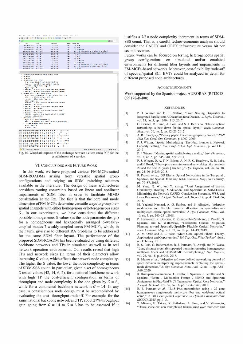
Fig. 15. Wireshark capture of the exchange between a client and a PCE for the

establishment of a service.

VI. CONCLUSIONS AND FUTURE WORK

In this work, we have proposed various FM-MCFs-suited SDM-ROADMs arising from versatile spatial group configurations and relying on SDM switching schemes available in the literature. The design of these architectures considers routing constraints based on linear and nonlinear impairments of SDM fiber in order to facilitate MIMO equalization at the Rx. The fact is that the core and mode dimension of FM-MCFs determine versatile ways to group their spatial channels with either homogenous or heterogeneous sizes 𝐺 . In our experiments, we have considered the different possible homogeneous 𝐺 values (as the node parameter design) for a homogeneous and hexagonally arranged 6-weakly-coupled modes 7-weakly-coupled cores FM-MCFs, which, in their turn, give rise to different RA problems to be addressed for the same SDM fiber layout. The performance of the proposed SDM-ROADM has been evaluated by using different backbone networks and TPs in simulated as well as in real network operation environments. Our results reveal that high TPs and network sizes (in terms of their diameter) allow increasing 𝐺 value, which affects the network node complexity. The higher the 𝐺 value, the lower the node complexity in terms of SDM-SSS count. In particular, given a set of homogeneous 𝐺 tested values (42, 14, 6, 2), for a national backbone network with high TP the cost-efficient configuration in terms of throughput and node complexity is the one given by 𝐺 6, while for a continental backbone network is 𝐺 14. In any case, a conscientious node design must be accomplished by evaluating the cost- throughput tradeoff. For example, for the same national backbone network and TP, about 27% throughput gain going from 𝐺 14 to 𝐺 6 has to be assessed if it

justifies a 7/3 node complexity increment in terms of SDM-SSS count. That is, a careful techno-economic analysis should consider the CAPEX and OPEX infrastructure versus bit per second revenue. Future works can be focused on testing heterogeneous spatial group configurations on simulated and/or emulated environments for different fiber layouts and impairments in FM-MCFs-based networks. Moreover, cost-flexibility trade-off of spectral/spatial SCh BVTs could be analyzed in detail for different proposed node architectures.

ACKNOWLEDGMENTS

Work supported by the Spanish project AURORAS (RTI2018-099178-B-I00)

REFERENCES [1] P. J. Winzer and D. T. Neilson, “From Scaling Disparities to

Integrated Parallelism: A Decathlon for a Decade,” J. Light. Technol., vol. 35, no. 5, pp. 1099–1115, 2017.

[2] O. Gerstel, M. Jinno, A. Lord, and S. J. Ben Yoo, “Elastic optical networking: A new dawn for the optical layer?,” IEEE Commun. Mag., vol. 50, no. 2, pp. 12–20, 2012.

[3] A. R. Chraplyvy, “Plenary paper: The coming capacity crunch,” 2009 35th Eur. Conf. Opt. Commun., p. 8007, 2009.

[4] P. J. Winzer, “Spatial Multiplexing : The Next Frontier in Network Capacity Scaling,” Eur. Conf. Exhib. Opt. Commun., p. We.1.D.1, 2013.

[5] P. J. Winzer, “Making spatial multiplexing a reality,” Nat. Photonics, vol. 8, no. 5, pp. 345–348, Apr. 2014.

[6] P. J. Winzer, D. A. T. N. Eilson, A. N. R. C. Hraplyvy, N. B. Labs, and H. Road, “Fiber-optic transmission and networking : the previous 20 and the next 20 years [ Invited ],” Opt. Express, vol. 26, no. 18, pp. 24190–24239, 2018.

[7] R. Proietti et al., “3D Elastic Optical Networking in the Temporal , Spectral , and Spatial Domains,” IEEE Commun. Mag., no. February, pp. 79–87, 2015.

[8] M. Yang, Q. Wu, and Y. Zhang, “Joint Assignment of Spatial Granularity, Routing, Modulation, and Spectrum in SDM-EONs: Minimizing the Network CAPEX Considering Spectrum, WSS, and Laser Resources,” J. Light. Technol., vol. 36, no. 18, pp. 4153–4166, 2018.

[9] M. Yaghubi-Namaad, A. G. Rahbar, and B. Alizadeh, “Adaptive modulation and flexible resource allocation in space-division- multiplexed elastic optical networks,” J. Opt. Commun. Netw., vol. 10, no. 3, pp. 240–251, 2018.

[10] P. Lechowicz, R. Goscien, R. Rumipamba-Zambrano, J. Perello, S. Spadaro, and K. Walkowiak, “Greenfield Gradual Migration Planning toward Spectrally-Spatially Flexible Optical Networks,” IEEE Commun. Mag., vol. 57, no. 10, pp. 14–19, 2019.

[11] A. M. Ortiz and R. L. Sáez, “Multi-Core Optical Fibers: Theory, Applications and Opportunities,” Sel. Top. Opt. Fiber Technol. Appl., no. February, 2018.

[12] R. S. Luís, G. Rademacher, B. J. Puttnam, Y. Awaji, and N. Wada, “Long distance crosstalk-supported transmission using homogeneous multicore fibers and SDM-MIMO demultiplexing,” Opt. Express, vol. 26, no. 18, p. 24044, 2018.

[13] R. Munoz et al., “Adaptive software defined networking control of space division multiplexing super-channels exploiting the spatial-mode dimension,” J. Opt. Commun. Netw., vol. 12, no. 1, pp. A58–A69, 2020.

[14] R. Rumipamba-Zambrano, J. Perello, S. Spadaro, J. Perelló, and S. Spadaro, “Route , Modulation Format , MIMO and Spectrum Assignment in Flex-Grid/MCF Transparent Optical Core Networks,” J. Light. Technol., vol. 36, no. 16, pp. 3534–3546, 2018.

[15] B. J. Puttnam et al., “2.15 Pb/s transmission using a 22 core homogeneous single-mode multi-core fiber and wideband optical comb,” in 2015 European Conference on Optical Communication (ECOC), 2015, pp. 1–3.

[16] T. Mizuno, H. Takara, K. Shibahara, A. Sano, and Y. Miyamoto, “Dense space division multiplexed transmission over multicore and

multimode fiber for long-haul transport systems,” J. Light. Technol., vol. 34, no. 6, pp. 1484–1493, 2016.

[17] T. Hayashi, T. Taru, O. Shimakawa, T. Sasaki, and E. Sasaoka, “Ultra-low-crosstalk multi-core fiber feasible to ultra-long-haul transmission,” 2011 Opt. Fiber Commun. Conf. Expo. Natl. Fiber Opt. Eng. Conf., pp. 1–3, 2011.

[18] T. Mizuno et al., “Long-Haul Dense Space-Division Multiplexed Transmission over Low-Crosstalk Heterogeneous 32-Core Transmission Line Using a Partial Recirculating Loop System,” J. Light. Technol., vol. 35, no. 3, pp. 488–498, 2017.

[19] J. Sakaguchi et al., “228-spatial-channel Bi-directional data communication system enabled by 39-core 3-mode fiber,” J. Light. Technol., vol. 37, no. 8, pp. 1756–1763, 2019.

[20] D. M. Marom and M. Blau, “Switching solutions for WDM-SDM optical networks,” IEEE Commun. Mag., vol. 53, no. 2, pp. 60–68, 2015.

[21] J. Sakaguchi et al., “SDM-WDM hybrid reconfigurable add-drop nodes for self-homodyne photonic networks,” 2013 IEEE Photonics Soc. Summer Top. Meet. Ser. PSSTMS 2013, vol. 2, pp. 117–118, 2013.

[22] N. Amaya et al., “Fully-elastic multi-granular network with space/frequency/time switching using multi-core fibres and programmable optical nodes,” Opt. Express, vol. 21, no. 7, p. 8865, Apr. 2013.

[23] B. Shariati et al., “Impact of spatial and spectral granularity on the performance of SDM networks based on spatial superchannel switching,” J. Light. Technol., vol. 35, no. 13, pp. 2559–2568, 2017.

[24] F. Arpanaei, N. Ardalani, H. Beyranvand, and S. A. Alavian, “Three-dimensional resource allocation in space division multiplexing elastic optical networks,” J. Opt. Commun. Netw., vol. 10, no. 12, pp. 959–974, 2018.

[25] G. P. Agrawal, S. Mumtaz, and R. J. Essiambre, “Nonlinear performance of sdm systems designed with multimode or multicore fibers,” Opt. Fiber Commun. Conf. OFC 2013, vol. 0, no. 2, pp. 12–14, 2013.

[26] C. Koebele et al., “40km transmission of five mode division multiplexed data streams at 100Gb/s with low MIMO-DSP complexity,” Opt. InfoBase Conf. Pap., pp. 39–41, 2011.

[27] J. Carpenter, B. C. Thomsen, and T. D. Wilkinson, “Degenerate Mode-Group Division Multiplexing,” vol. 30, no. 24, pp. 3946–3952, 2012.

[28] F. Feng et al., “High-Order Mode-Group Multiplexed Transmission over a 24km Ring-Core Fibre with OOK Modulation and Direct Detection,” Eur. Conf. Opt. Commun. ECOC, vol. 2017-September, no. 1, pp. 1–3, 2017.

[29] M. Jiang et al., “Weakly coupled 4-mode step-index FMF and demonstration of IM/DD MDM transmission,” in 17th International Conference on Optical Communications and Networks (ICOCN2018), 2019, vol. 11048, p. 72.

[30] J. Li et al., “Weakly-coupled mode division multiplexing over conventional multi-mode fiber with intensity modulation and direct detection,” Frontiers of Optoelectronics, vol. 12, no. 1. Higher Education Press, pp. 31–40, 01-Mar-2019.

[31] C. Rottondi, P. Boffi, P. Martelli, and M. Tornatore, “Routing, Modulation Format, Baud Rate and Spectrum Allocation in Optical Metro Rings with Flexible Grid and Few-Mode Transmission,” J. Light. Technol., vol. 35, no. 1, pp. 61–70, Jan. 2017.

[32] T. Hayashi et al., “Six-Mode 19-Core Fiber with 114 Spatial Modes for Weakly-Coupled Mode-Division-Multiplexed Transmission,” J. Light. Technol., vol. 35, no. 4, pp. 748–754, 2017.

[33] K. Shibahara et al., “Dense SDM (12-Core × 3-Mode) transmission over 527 km with 33.2-ns mode-dispersion employing low-complexity parallel MIMO frequency-domain equalization,” J. Light. Technol., vol. 34, no. 1, pp. 196–204, 2016.

[34] Y. Sasaki, K. Takenaga, S. Matsuo, K. Aikawa, and K. Saitoh, “Few-mode multicore fibers for long-haul transmission line,” Opt. Fiber Technol., vol. 35, pp. 19–27, 2017.

[35] M. Kasahara, K. Saitoh, T. Sakamoto, N. Hanzawa, and T. Matsui, “Design of Three-Spatial-Mode Ring-Core Fiber,” vol. 32, no. 7, pp. 1337–1343, 2014.

[36] R. Maruyama, N. Kuwaki, S. Matsuo, and M. Ohashi, “Experimental investigation of relation between mode-coupling and fiber characteristics in few-mode fibers,” in Conference on Optical Fiber Communication, Technical Digest Series, 2015, vol. 2015-June, p. M2C.1.

[37] R. Munoz et al., “SDN control of sliceable multidimensional (spectral and spatial) transceivers with YANG/NETCONF,” J. Opt. Commun. Netw., vol. 11, no. 2, pp. A123–A133, 2019.

[38] K. Saitoh and S. Matsuo, “Multicore fiber technology,” J. Light. Technol., vol. 34, no. 1, 2016.

[39] R. Ryf et al., “Mode-division multiplexing over 96 km of few-mode fiber using coherent 6×6 MIMO processing,” J. Light. Technol., vol. 30, no. 4, pp. 521–531, 2012.

[40] S. Randel et al., “6×56-Gb/s mode-division multiplexed transmission over 33-km few-mode fiber enabled by 6×6 MIMO equalization,” Opt. Express, vol. 19, no. 17, p. 16697, 2011.

[41] S. Mumtaz, R. J. Essiambre, and G. P. Agrawal, “Nonlinear propagation in multimode and multicore fibers: Generalization of the Manakov equations,” J. Light. Technol., vol. 31, no. 3, pp. 398–406, 2013.

[42] M. Ruiz et al., “Planning fixed to flexgrid gradual migration: Drivers and open issues,” IEEE Commun. Mag., vol. 52, no. 1, pp. 70–76, 2014.

[43] M. Jinno and Y. Mori, “Unified Architecture of an Integrated SDM-WSS Employing a PLC-Based Spatial Beam Transformer Array for Various Types of SDM Fibers,” J. Opt. Commun. Netw., vol. 9, no. 2, p. A198, 2017.

[44] R. Rumipamba-Zambrano, F.-J. Moreno-Muro, J. Perelló, P. Pavón-Mariño, and S. Spadaro, “Space continuity constraint in dynamic Flex-Grid/SDM optical core networks: An evaluation with spatial and spectral super-channels,” Comput. Commun., vol. 126, 2018.

[45] D. M. Marom et al., “Survey of Photonic Switching Architectures and Technologies in Support of Spatially and Spectrally Flexible Optical Networking [Invited],” J. Opt. Commun. Netw., vol. 9, no. 1, p. 1, Jan. 2017.

[46] Y. Cao et al., “Mode conversion-based crosstalk-aware routing, spectrum and mode assignment in space-division multiplexing elastic optical networks,” ICOCN 2017 - 16th Int. Conf. Opt. Commun. Networks, vol. 2017-Janua, no. 1, pp. 1–3, 2017.

[47] N. K. Fontaine et al., “Few-Mode Fiber Wavelength Selective Switch with Spatial-Diversity and Reduced-Steering Angle,” Opt. Fiber Commun. Conf., no. c, pp. 3–5, 2014.

[48] D. M. Marom et al., “Wavelength-selective switch with direct few mode fiber integration,” Opt. Express, vol. 23, no. 5, p. 5723, 2015.

[49] K. Ho, S. Member, J. M. Kahn, and J. P. Wilde, “Wavelength-Selective Switches for Mode-Division Multiplexing : Scaling and Performance Analysis,” pp. 1–13, 2014.

[50] L. E. Nelson et al., “Spatial superchannel routing in a two-span ROADM system for space division multiplexing,” J. Light. Technol., vol. 32, no. 4, pp. 783–789, 2014.

[51] T. Sakamoto et al., “Six-Mode Seven-Core Fiber for Repeated Dense Space-Division Multiplexing Transmission,” J. Light. Technol., vol. 36, no. 5, pp. 1226–1232, 2018.

[52] A. E. Elfiqi, A. A. I. Ali, Z. A. El-Sahn, K. Kato, and H. M. H. Shalaby, “Theoretical analysis of long-haul systems adopting mode-division multiplexing,” Opt. Commun., vol. 445, no. March, pp. 10–18, 2019.

[53] P. Poggiolini, G. Bosco, A. Carena, V. Curri, Y. Jiang, and F. Forghieri, “The GN-Model of Fiber Non-Linear Propagation and its Applications,” J. Light. Technol., vol. 32, no. 4, pp. 694–721, Feb. 2014.

[54] T. Hayashi, T. Taru, O. Shimakawa, T. Sasaki, and E. Sasaoka, “Uncoupled multi-core fiber enhancing signal-to-noise ratio.,” Opt. Express, vol. 20, no. 26, pp. B94-103, 2012.

[55] K. Walkowiak, M. Klinkowski, and P. Lechowicz, “Dynamic Routing in Spectrally Spatially Flexible Optical Networks with Back-to-Back Regeneration,” J. Opt. Commun. Netw., vol. 10, no. 5, p. 523, May 2018.

[56] B. Shariati, A. Mastropaolo, N. P. Diamantopoulos, J. M. Rivas-Moscoso, D. Klonidis, and I. Tomkos, “Physical-layer-aware performance evaluation of SDM networks based on SMF bundles, MCFs, and FMFs,” J. Opt. Commun. Netw., vol. 10, no. 9, pp. 712–722, 2018.

[57] J. Perelló, J. M. Gené, A. Pagès, J. A. Lazaro, and S. Spadaro, “Flex-Grid/SDM Backbone Network Design with Inter-Core XT-Limited Transmission Reach,” J. Opt. Commun. Netw., vol. 8, no. 8, p. 540, Aug. 2016.

[58] R. Rumipamba-Zambrano, J. Perelló, J. M. Gené, and S. Spadaro, “Cost-effective spatial super-channel allocation in Flex-Grid/MCF optical core networks,” Opt. Switch. Netw., vol. 27, pp. 93–101, Jan.

2018. [59] R. Rumipamba-Zambrano, J. Perelló, and S. Spadaro, “Dynamic

Traffic Grooming in Joint Switching ( JoS ) -enabled Flex-Grid / SDM Optical Core Networks,” in European Conference on Optical Communication, 2018, no. 1, pp. 2–4.

[60] “RFC 8283 - An Architecture for Use of PCE and the PCE Communication Protocol (PCEP) in a Network with Central Control.” [Online]. Available: https://tools.ietf.org/html/rfc8283. [Accessed: 14-Jan-2020].

[61] R. Martínez, R. Casellas, R. Vilalta, and R. Muñoz, “Distributed vs. Centralized PCE-based Transport SDN Controller for Flexi-Grid Optical Networks,” in Optics InfoBase Conference Papers, 2017, vol. 7, pp. 6–8.

[62] “RFC 7699 - Generalized Labels for the Flexi-Grid in Lambda Switch Capable (LSC) Label Switching Routers.” [Online]. Available: https://tools.ietf.org/html/rfc7699. [Accessed: 14-Jan-2020].

design and assessment of fm-mcfs-suited sdm-roadms with

Documents