design and construction of a fluidized bed

University of North DakotaUND Scholarly Commons

Theses and Dissertations Theses, Dissertations, and Senior Projects

January 2013

Design And Construction Of A Fluidized BedRobert Ryan Mota

Follow this and additional works at: https://commons.und.edu/theses

This Thesis is brought to you for free and open access by the Theses, Dissertations, and Senior Projects at UND Scholarly Commons. It has beenaccepted for inclusion in Theses and Dissertations by an authorized administrator of UND Scholarly Commons. For more information, please [email protected].

Recommended CitationMota, Robert Ryan, "Design And Construction Of A Fluidized Bed" (2013). Theses and Dissertations. 1575.https://commons.und.edu/theses/1575

https://commons.und.edu?utm_source=commons.und.edu%2Ftheses%2F1575&utm_medium=PDF&utm_campaign=PDFCoverPages

https://commons.und.edu/theses?utm_source=commons.und.edu%2Ftheses%2F1575&utm_medium=PDF&utm_campaign=PDFCoverPages

https://commons.und.edu/etds?utm_source=commons.und.edu%2Ftheses%2F1575&utm_medium=PDF&utm_campaign=PDFCoverPages

https://commons.und.edu/theses?utm_source=commons.und.edu%2Ftheses%2F1575&utm_medium=PDF&utm_campaign=PDFCoverPages

https://commons.und.edu/theses/1575?utm_source=commons.und.edu%2Ftheses%2F1575&utm_medium=PDF&utm_campaign=PDFCoverPages

mailto:[email protected]

DESIGN AND CONSTRUCTION OF A FLUIDIZED BED

by

Robert Ryan Mota

Bachelor of Science, California State Polytechnic University, Pomona, 2010

A Thesis

Submitted to the Graduate Faculty

of the

University of North Dakota

in partial fulfillment of the requirements

for the degree of

Masters of Science

Grand Forks, North Dakota

December

2013

ii

This thesis, submitted by Robert Ryan Mota in partial fulfillment of the requirements for the

Degree of Master of Science from the University of North Dakota, has been read by the Faculty

Advisory Committee under whom the work has been done and is hereby approved.

____________________________________

Dr. Steven A Benson, Chairperson

____________________________________

Dr. Gautham Krishnamoorthy

____________________________________

Dr. Michael D. Mann

This thesis meets the standards for appearance, conforms to the style and format

requirements of the Graduate School of the University of North Dakota, and is hereby approved.

____________________________________

Dr. Wayne Swisher

Dean of the Graduate School

____________________________________

Date

iii

PERMISSION

Title Design and Construction of a Fluidized Bed

Department Chemical Engineering

Degree Masters of Science

In presenting this thesis in partial fulfillment of the requirements for a graduate degree

from the University of North Dakota, I agree that the library of this University shall make it

freely available for inspection. I further agree that permission for extensive copying for

scholarly purposes may be granted by the professor who supervised my thesis work or, in his

absence, by the chairperson of the department or the dean of the Graduate School. It is

understood that any copying or publication or other use of this thesis or part thereof for financial

gain shall not be allowed without my written permission. It is also understood that due

recognition shall be given to me and to the University of North Dakota in any scholarly use

which may be made of any material in my thesis.

Signature ________________________

Robert R. Mota

Date 12-4-2013

iv

TABLE OF CONTENTS

LIST OF FIGURES ....................................................................................................................... ix

LIST OF TABLES ....................................................................................................................... xiii

ABSTRACT ...................................................................................................................... xviii

CHAPTER

I. INTRODUCTION ........................................................................................................................1

1.1 Objective ....................................................................................................................1

1.2 Scope .......…………………………………………………………………………...1

1.3 Motivation ..................................................................................................................1

II. LITERATURE REVIEW ............................................................................................................4

2.1 Introduction................................................................................................................4

2.2 Background information ............................................................................................6

2.2. Thermodynamics and kinetics of gasification ...........................................................6

2.3 Types of reactors ......................................................................................................10

2.3.1 Entrained flow gasifier ...............................................................................10

2.3.2 Moving bed gasifier ...................................................................................12

2.3.3 Fluidized bed reactor .................................................................................14

2.4 Fuel quality and fuel properties ...............................................................................16

2.4.1 Lignite coal ................................................................................................18

2.5 Impurity transformations .........................................................................................23

2.6 Impacts of impurities................................................................................................25

v

2.7 Measures to minimize impurities .............................................................................26

2.7. Alternative bed materials .............................................................................26

2.7.2 Mineral additives .......................................................................................27

2.7.3 Pretreating coals ........................................................................................27

2.7.4 Blending of coals........................................................................................27

2.8 Applications .............................................................................................................28

2.8.1 Fuel Production .........................................................................................29

2.8.1.1 Methane...................................................................................................29

2.8.1.2 Methonol .................................................................................................29

2.8.1.3 Fischer-Trospsch synthesis .....................................................................29

2.8.2 Chemical Production .................................................................................30

2.8.2.1 Ammonia .................................................................................................30

2.8.3 Hydrogen Production.................................................................................30

2.8.4 Power generation .......................................................................................31

2.9 Summary ..................................................................................................................33

III. DETAILED DESIGN OF A FLUIDIZED BED AND ITS ASSOCIATED UNIT

OPERATIONS FOR COAL COMBUSTION AND GASIFICATION .......................................34

3.1 Introduction..............................................................................................................34

3.2 Fluidized bed design ................................................................................................36

3.2.1 Fluidization Calculations ..........................................................................36

3.2.1.1 Minimum Fluidization velocity ...................................................39

3.2.1.2 Operating Velocity ......................................................................40

3.2.1.3 Characterizing the fluidization in the reactor ............................41

3.2.1.4 Slugging Velocity ........................................................................42

vi

3.2.1.5 Bed Height ...................................................................................44

3.2.1.6 Terminal Velocity ........................................................................45

3.2.1.7 Fluidization Summary .................................................................46

3.2.1.8 Reactor Diameter ........................................................................46

3.2.2 Combustion Calculations ...........................................................................47

3.2.2.1 Reactor Power Requirements ......................................................50

3.2.2.2 Reactor Height ............................................................................50

3.2.2.3 Combustion Calculations Summary ............................................51

3.2.3 Distributor Plate Design ............................................................................52

3.3 Simulation ................................................................................................................57

3.4 Fluidized Bed Design Summary ...............................................................................60

3.5 Design of Corresponding Unit Operations ..............................................................61

3.5.1 Pregasification Unit Operations ................................................................61

3.5.1.1 Air Pre-Heater ............................................................................62

3.5.1.2 Steam Generator .........................................................................62

3.5.1.3 Coal Feeder .................................................................................63

3.5.2 Syngas Cleanup Unit Operations, Post gasification ..................................64

3.5.2.1 Cyclone ........................................................................................64

3.5.2.2 Heat Exchangers .........................................................................67

3.6 Summary ...................................................................................................................73

IV. EXPERIMENTAL .....................................................................................................................76

4.1 Introduction ..............................................................................................................76

4.2 Design of Process .....................................................................................................76

vii

4.3 Construction .............................................................................................................78

4.3.1 Unit Operations ..........................................................................................78

4.3.1.1 Air Preheater ...............................................................................78

4.3.1.2 Steam Generator .........................................................................79

4.3.1.3 Coal Feeder .................................................................................79

4.3.1.4 Fluidized Bed Reactor.................................................................80

4.3.1.5 Cyclone ........................................................................................80

4.3.1.6Heat Exchangers ..........................................................................81

4.3.2 Controls......................................................................................................82

4.3.3 Operating Issues ........................................................................................83

4.3.3.1 Thermal Expansion of the Bed ....................................................83

4.3.3.2 Thermocouple Problem ...............................................................87

4.4 Ash Sampling System ...............................................................................................88

4.5 Commissioning of the System...................................................................................90

4.5.1 Fluidization Experiments ...........................................................................90

4.5.2 Shakedown Experiments ............................................................................94

4.5.2.1 Combustion Experiments ............................................................94

4.5.2.1.1 Oxygen Combustion .................................................96

4.5.2.1.2 Carbon Conversion ..................................................96

4.5.2.2 Hydro-gasification ......................................................................97

4.5.3 Tar Formation ............................................................................................99

4.5.4 Bed Agglomeration Formation ................................................................103

4.5.5 Summary ...................................................................................................105

viii

V. RESULTS AND DISCUSSION .............................................................................................106

5.1 Introduction................................................................................................................106

5.2 Air Gasification ..........................................................................................................106

5.3 Oxygen Gasification...................................................................................................113

5.4 Oxygen gasification summary ....................................................................................119

5.5 Agglomerate Generation ............................................................................................120

5.5.1Agglomerate Sample Preparation................................................................120

5.5.2 Combustion Generated Agglomerates ........................................................122

5.5.3 Gasification Agglomerates..........................................................................124

5.6 Summary ....................................................................................................................167

VI. CONCLUSIONS ...................................................................................................................169

VII. RECOMMENDATIONS FOR FUTURE WORK ...............................................................171

Appendix A: Standard Operating Procedure for the fluidized bed gasifier .................................175

Appendix B: Loss on Ignition Tables ..........................................................................................186

Appendix C: Temperature profiles of the reactor for gasification experiments. .........................187

Appendix D: Coal Feeder Calibration .........................................................................................190

Appendix E: Steam Calibration ...................................................................................................195

Appendix F: Hydrogen sulfide concentration for air blown gasification …………………..196

Appendix G: Fuel properties of lignite: Ultimate, Proximate and Mineral analysis………..….197

REFERENCES ........................................................................................................................198

ix

LIST OF FIGURES

Figure Page

1. Reaction Sequence for gasification of coal ......................................................................... 7

2. The influence of Heating Rate on Gasification. .................................................................. 8

3. Reaction Rates in Temperature Zones. ............................................................................... 9

4. Texaco’s Entrained Flow Gasifier .................................................................................... 12

5. Bed Gasifier operating in Dry-Ash Mode ......................................................................... 13

6. Depiction of a fluidized bed. ............................................................................................. 15

7. Chemical and Physical Properties of Coals in the Various Rank Classes ....................... 17

8. Description of ash formation in the gasification process. ................................................ 21

9. Impurity buildup of slag and temperature profile between

the furnace and slag layer ................................................................................................. 24

10. Schematic of Applications for gasification ....................................................................... 28

11. Comparison of efficiencies for power generation of low and high ranked coals ............. 32

12. Process flow diagram of the gasification process. ............................................................ 37

13. Fluidizing mapping regime. .............................................................................................. 42

14. Distributor plate pressure versus superficial gas velocity. ................................................ 55

15. ASPEN simulation model of gasification process. ........................................................... 58

16. Depiction of a cyclone. ..................................................................................................... 65

17. Schematic of the shell and tube heat exchanger with baffles. .......................................... 69

18. Cocurrent flow regime for heat exchanger. ...................................................................... 70

x

19. Counter current flow for a heat exchanger. ...................................................................... 71

20. Baffle configuration for the inlet of the heat exchanger. .................................................. 72

21. Baffle configuration for the outlet of the heat exchanger. ................................................ 73

22. Constructed fluidized bed reactor sytem. .......................................................................... 77

23. Coal Feeding system. ........................................................................................................ 84

24. Pneumatic sand replenishing system. ............................................................................... 85

25. Bypass system for ash and char sample collection from the cyclone. .............................. 89

26. Fluidization experiment, pressure drop Vs velocity at ambient conditions. ..................... 91

27. Fluidization experiment, pressure drop Vs velocity at operating conditions.................... 92

28. Theoretical velocity versus pressure drop across the bed. ................................................ 92

29. Combustion shakedown experiment: flue-gas composition

at different coal feedrates .................................................................................................. 95

30. Oxygen combustion experiment. ...................................................................................... 96

31. Carbon Conversion in different combustion experiments. ............................................... 97

32. Hydro-gasification shakedown experiment. ..................................................................... 98

33. Loss on Ignition analysis of lignite coal. ........................................................................ 100

34. Liquid samples collected at different gasification conditions......................................... 101

35. TGA/DSC analysis of a liquid sample under gasification conditions. ........................... 102

36. TGA analysis on a tar sample collected under gasification conditions. ......................... 103

37. Agglomeration formation under combustion conditions. ............................................... 104

38. Air gasification: Syngas composition Vs. carbon to oxygen ratio.................................. 107

39. Air gasification: Carbon conversion at different carbon to oxygen ratios. ..................... 111

40. Air blown gasification: Cold gas efficiency versus carbon to oxygen ratio. ................. 112

41. Oxygen gasification: Syngas composition versus oxygen to carbon ratio. .................... 113

xi

42. Gasification: carbon conversion versus oxygen to carbon ratio. .................................... 115

43. Oxygen gasification: Cold gas efficiency at different oxygen to carbon ratios. ............. 116

44. Oxygen gasification: Syngas composition versus steam to carbon ratio. ....................... 117

45. Oxygen gasification: syngas composition versus steam to carbon ratio......................... 118

46. Polished agglomerate samples before carbon coat. ........................................................ 121

47. Backscattered electron images of combustion generated impurities

showing morphology analysis points. ............................................................................. 124

48. Backscattered electron images of air gasification(1-1B) generated

impurities showing morphology analysis points. ........................................................... 126

49. Backscattered electron images of air gasification(1-1B) generated


50. Backscattered electron images of Air gasification (1-1C) generated

impurities showing SEMPC analysis grids. .................................................................... 128

51. Ternary Diagram of SEMPC of sample 1-1C ................................................................. 129

52. Backscattered electron images of air gasification (1-1F) generated


53. Backscattered electron images of Air gasification (1-1F) generated

impurities showing SEMPC analysis grids. .................................................................... 133

54. Ternary Diagram of SEMPC of sample 1-1F. ................................................................ 134

55. Backscattered electron images of air gasification (11-1B) generated


56. Backscattered electron images of oxygen gasification (12-1) generated


57. Backscattered electron images of Oxygen gasification (12-1) generated

impurities showing SEMPC analysis grids ..................................................................... 138

58. Ternary Diagram of SEMPC of sample 12-1 ................................................................. 139



xii


impurities showing morphology analysis points. ........................................................... 143 61. `Backscattered electron images of gasification (2-1) generated


62. Backscattered electron images of gasification (2-3) generated








66. Ternary Diagram of SEMPC of sample 2-6 ................................................................... 152





69. Ternary Diagram of SEMPC of sample 2-9 ................................................................... 156

70. Network modifiers creating non-bridging oxygen atoms. .............................................. 158

71. Viscous flow sintering of particles. ................................................................................ 159

72. Viscosity prediction of lignite using Kalmanovitch viscosity prediction model. .......... 161

73. Viscosity calculations of unclassified point count data. ................................................. 163

xiii

LIST OF TABLES

Table Page

1. Summary of fluidization calculations ............................................................................... 46

2. Predicted coal consumption based on different reactor sizes ........................................... 47

3. Summary of combustion calculations. .............................................................................. 52

4. Design criteria for distributor plate ................................................................................... 57

5. Aspen simulation results of gasification simulation. ........................................................ 59

6. Fluidized bed design summary. ........................................................................................ 61

7. Lapple method for cyclone dimensions. ........................................................................... 66

8. Summary of cyclone design parameters

9. Comparison of theoretical and experimental fluidization values

at ambient and operating conditions. ................................................................................. 93

10 Syngas comparison between hydro-gasifcation and literature values. .............................. 98

11.Syngas composition of air blown gasification comparison to TRIGTRIG. .................... 108

12. Confidence intervals for air gasification. ........................................................................ 110

13. Comparison of UND data with TRIG for oxygen blown gasification. ........................... 114

14. Comparison of carbon conversion and cold gas efficiency ............................................ 117

15. Morphology analysis results of Combustion Generated impurities.

Elemental results expressed as weight percent, normalized to 100%. .................................. 123

16. Morphology analysis results of Air Gasification (1-1B) Generated impurities.


17. Morphology analysis results of Air Gasification (1-1C) Generated impurities.


xiv

18. SEMPC analysis results of Air Gasification (1-1C). Results expressed as

weight percent, normalized to 100%. ................................................................................... 128

19. SEMPC elemental results of Air Gasification (1-1C). Elemental results

expressed as weight percent, normalized to 100%. .............................................................. 129

20. Morphology analysis results of Air Gasification (1-1F) Generated impurities.


21. SEMPC analysis results of Air Gasification (1-1F). Results expressed as


22. SEMPC elemental results of Air Gasification (1-1F). Elemental results


23. Morphology analysis results of Air Gasification (11-1B) Generated impurities.


24. Morphology analysis results of Oxygen Gasification (12-1) Generated impurities.


25. SEMPC analysis results of Oxygen Gasification (12-1). Results expressed

as weight percent, normalized to 100%. ............................................................................... 138

26. SEMPC elemental results of Oxygen Gasification (12-1). Elemental

results expressed as weight percent, normalized to 100%. ................................................... 138





29. Morphology analysis results of Gasification (2-1) Generated impurities.








xv

33. SEMPC analysis results of Gasification (2-6). Results expressed as


34. SEMPC elemental results of Gasification (2-6). Elemental results




36. SEMPC analysis results of Gasification (2-9). Results expressed as


37. SEMPC elemental results of Gasification (2-9). Elemental results


38. ASTM mineral analysis of coal. ..................................................................................... 162

39. CCSEM analysis of Center lignite coal. ......................................................................... 166

xvi

ACKNOWLEDGEMENTS

I would like to thank the department of chemical engineering for giving me the

opportunity to do research. I would like to thank my advisor Dr. Steve Benson for all of his

guidance, support and patience. I would like to thank my advisory committee members, Dr.

Michael Mann and Dr. Gautham Krishnamoorthy for their guidance and support. I am grateful

for the UND chemical engineering department faculty; each of them has helped me in some way

along my journey. I would like to thank the Department of Energy Epscor-who funded the

project.

I am grateful to staff and resources at Microbeam technologies for allowing me to use

their equipment to analyze my work, and for the guidance and assistance. I would also like to

acknowledge the work both Harry Feilen and David Hirschmann did towards my project.

Finally, I would like to thank all other people who have contributed directly or indirectly to my

research that I am unable to thank individually.

xvii

I would like to dedicate my master’s thesis to my loving parents, Robert and Julie as well as

my sister, Jacquelyn and brother, Vincent for all of their love and support.

xviii

ABSTRACT

Coal combustion is responsible for the majority of electricity production in the United

States. It is however, also the primary cause for carbon dioxide emissions, which contribute to

global warming. With oil reaching its peak production in the near future, alternative fuel sources

will be needed to meet the worlds growing energy demands. Coal is an abundant resource that

has the potential to meet those demands. In contrast to coal combustion, coal gasification only

partially oxidizes the coal to produce a syngas containing of hydrogen and carbon monoxide,

which means less carbon dioxide emissions. Utilizing coal in gasification technologies is the key

to using coal in a more environmentally friendly way. Coal utilized gasification technologies

have a variety of different applications. These applications include production of synthetic

natural gas, production of methanol, to converting the syngas to gasoline, or chemicals like

ammonia or a more efficient method to produce electricity for power generation. There are some

challenges associated with coal when trying to extract its energy. These challenges exist due to

the impurities that are inherent in coal. These impurities get released upon combustion and

gasification systems and cause corrosion and erosion which can lead to damaging of expensive

equipment used in chemical processing plants. Therefore research is needed to address these

challenges, in order to improve the gasification systems so they can become more efficient. One

area of gasification technology that can utilize coal to generate useful products is fluidized bed

gasification. Fluidized bed gasification is not as widely used as other gasification technologies in

industry. This is because these systems have their own unique set of challenges associated with

xix

them. This research is focused on fluidized bed gasification with lignite as the design fuel. In

this work a fluidized bed gasifier was designed, constructed, commissioned and optimized for

hydrogen production. The design was based off of the literature and centered on the minimum

fluidization velocity. Shakedown experiments were performed as part of commissioning the

system. Experiments were run under combustion conditions, air blown gasification, oxygen

blown gasification, oxygen combustion, and a hydrogen retort. A hydrogen rich syngas was

produced, containing 58% hydrogen for the retort experiments and as high as 55% for oxygen

blown gasification. This hydrogen rich stream was largely because of the water gas shift

reaction that took place downstream of the gasifier. Along with these experiments, deposits from

the impurities were formed under realistic conditions. The deposits were prepared and analyzed

using scanning electron microscopy. The two methods which were used to characterize the

deposits were morphology, which uses EDS to identify the atoms present in the sample, and

point count (SEMPC) which uses a computer program to compare and classify the mineral

phases present in the sample. Based on the results of the SEMPC analysis the mechanism from

which the deposits formed was through viscous flow sintering. The atomic species most

responsible for the sintering was found to be organically associated sodium and calcium in the

lignite.

1

CHAPTER I

INTRODUCTION

1.1 Objective

The objective of this research is to learn about gasification systems by designing and

constructing a fluidized bed gasifier with Lignite coal as the design fuel.

1.2 Scope

The scope of this project is design a fluidized bed for the gasification of lignite based on the

literature. Once that design is determined to be valid, the system will be constructed and

commissioned. The system will consist of a fluidized bed gasifier, along with post gasification

cleanup systems. Gasification experiments will be performed and behavior of the system will

analyzed including syngas composition, carbon conversion, cold gas efficiency, tar formation,

and impurity generation.

1.3 Motivation

With Oil prices being higher than ever, there is a new interest in developing green/alternative

energy technologies. Historically, compared to other types of alternative energy, petroleum

derived fuels have dominated the energy market, and realistically will continue to dominate the

energy market for the foreseeable future. Coal, like oil, is a fossil fuel and is the main source for

the majority of the world’s electricity. Coal is an abundant energy resource that will play an

important role in future energy requirements(Annual Energy Outlook 2011, 2011). The U.S has

a large amount of coal reserves that will last for a couple hundred years. In fact, in 2010 the

United States used coal to generate 46% of its total power, and reflects a 4.5% increase in coal

usage from the previous year(World Energy Council, 2013). This makes the utilization of coal

as an energy resource attractive due to its high abundance worldwide, and low cost. However, a

2

lot of the coal in the U.S is lignite, which is a low ranked coal that has not been used as much for

energy applications as its high rank counterparts. This is partly due to the inherent problems that

are associated with lignite that prevent technology from being further developed for its use.

Specifically lignite has a high moisture content, as well as large amounts of alkali metals namely

sodium, that can cause a lot of fouling of equipment and other problems.(Matsuoka, Suzuki,

Eylands, Benson, & Tomita, 2006). Coal presents some environmental challenges; it can create

pollution and contribute to global warming by releasing carbon dioxide into the atmosphere. The

utilization of coal is very versatile; coal can be used to produce chemicals, in electricity

production, and the production of hydrogen. One of the technologies that can utilize coal in a

more productive was is a process known as gasification. Gasification is a process in which turns

any material with a high carbon content, into a gaseous fuel with a heating value. It is a process

which is similar to combustion; however, gasification limits the amount of oxygen that is

available to react with fuel source, which creates a reducing environment. Ultimately, the

product gas in gasification is known as a syngas, and typically contains hydrogen and carbon

monoxide. There are different types of coals, each one with its own unique properties. The

unique properties of each coal present with it different problems and challenges that need to be

overcome. Depending on the application that is desired, for example, the production of

chemicals, hydrogen or electricity, as well as the availability, will determine the type of coal to

be used. Once the type of coal is selected, this will dictate the type reactor that will be

implemented to carry out the gasification process. Although the type of reactor does depend on

the type of coal being used there is an underlying common problem that affects each type of

gasification process in its own unique way that is the impurities in the coal. This work will show

how gasification, fluidized bed technology, along with coal can provide cleaner and more

3

efficient ways to utilize energy in the future. It will also provide a brief history on gasification,

what gasification is, and what its applications are and address some of the problems that

researchers are trying to overcome. As well go through actually designing, constructing and

commissioning of the fluidized bed system, present and interpret the data and offer

recommendations for future work.

4

CHAPTER II

2. LITERATURE REVIEW

2.1 Introduction

Gasification is a technology that has been around for a long time. In its most primitive

sense, humans have utilized gasification since we have figured out how to control fire and use it

to burn wood to keep ourselves warm (C. Higman, 2003). Over time different types of fuel have

been used, however the process has essentially remained unchanged. What exactly is

gasification? There have been two dominant definitions have evolved over the years. The first

by Higman and Van der Burgt, which is that gasification is a process where any carbonaceous

fuel is converted to a gaseous product with a heating value. Under this definition, such processes

as pyrolysis, partial oxidation, and hydrogenation are included (C. Higman, 2003). It should be

noted that this definition excludes combustion because during the combustion process, the

product fuel gas has no residual heating value. However, Berkowitz defines gasification

differently, and makes a sharp distinction between it and other process (Berkowitz, 1979). The

key point in Berkowitz’s definition of gasification is that all of the organic material in coal is

converted a gaseous form. Equally important, with this definition, only coal rank and

temperature affect the rate of gasification (Berkowitz, 1979). A simpler way of looking at

gasification is this: it is a process where fuel is burned in a reducing environment that is the

amount of oxygen that is burning the fuel is very limited, so that the products are not fully

oxidized. In any case when the carbon-rich fuel is gasified, the end result is a mixture of gasses

5

consisting of carbon monoxide and hydrogen which together is known as syn-gas

(C. Higman, 2013). In the gasification process, many different feedstock’s’ can be

utilized for energy (Minchener, 2005). The first fuel to be used was wood, although

wood was also needed for other applications, and became scarce. It was during the

beginning of the industrial revolution where a new type of fuel would be needed, so coal

started to be utilized for the purpose of heating and lighting. The production of town gas

is where gasification founds its niche in providing itself useful towards society. The

main purpose of town gas was for town illumination. Other applications that followed

were heating, the use as a raw material in the chemical industry and power generation.

One of the initial drawbacks of the town gas is that it had a low heating value which

could not provide much heat to utilize over long distances (C. Higman, 2003). This

combined with other technologies emerging such as the light bulb, put gasification on the

backburner of wide commercial use. At the heart of gasification carbon reacts with

oxygen and steam to produce hydrogen and carbon monoxide which can be summarized

in the chemical equation of the overall process below:

C + H2O H2 + CO

This is, however, an oversimplification of the gasification process. Gasification consists

of many steps and side reactions, all of which help determine the quality and composition

of the syngas. Usually gasification is described with six sets of reactions. They are the

combustion reactions, steam gasification reaction, Boudouard reaction, water gas shift

reaction, methanation reaction and hydro-gasification reaction. Their chemical equations

with associated enthalpies can be seen in the equations that follow:

1. Combustion reactions:

6

C + O2 CO2 ΔH= - 16900 BTU/lb-mol

C + 1/2O2 CO ΔH= - 47,600 BTU/lb-mol

CO + 1/2O2 CO2 ΔH= - 121,700 BTU/lb-mol

2. Steam gasification reaction:

C + H2O CO + H2 ΔH= 56,490 BTU/lb-mol

3. Boudouard reaction:

CO2 + C 2CO ΔH= + 74200 BTU/lb-mol

4. Water gas shift reaction:

CO + H2O CO2 + H2 ΔH= - 17,700 BTU/lb-mol

5. Methanation reaction:

CO + 3H2 CH4 + H2O ΔH= - 88,700 BTU/lb-mol

6. Hydro-gasification reaction:

2H2 + C CH4 ΔH= - 32,200 BTU/lb-mol

The water gas shift reaction plays an important role in converting the syngas to a

hydrogen rich stream. The chemical composition of the syngas will depend on the

operating conditions, residence times and chemical kinetics (S. A. Benson & Sondreal,

n.d.)

2.2 Background information

2.2.1 Thermodynamics and kinetics of gasification

Gasification can be a very complex process; this is due to the fact that usually the

carbonaceous material contains other materials within it such as impurities that can affect

the chemistry of the gasification process. The chemistry of gasification can be described

7

by thermodynamics, which is what will happen at certain conditions of temperature and

pressure and kinetics, which is what route will the reactions take and how fast do the

chemical reactions occur. Thermodynamically steam gasification takes place at 850 °C

and above, anything below that is considered pyrolysis (C. Higman, 2003). Despite the

fuel type, gasification exhibits the following reactions: Pyrolysis and tar cracking,

combustion reactions, steam gasification, secondary reactions, the water gas shift reaction

and methanation reactions. The most notable of the secondary reactions that take place in

the gasification process is the Boudouard reaction. Due to the fact that the initial steps of

pyrolysis and tar cracking are endothermic, heat must be provided by an outside source,

and thus makes the overall gasification process endothermic (S. A. Benson & Sondreal,

n.d.). The water-gas shift and methanation reactions are exothermic which contributes to

the energy balance at lower temperatures (chemical reaction 4). Figure 1 depicts the

general steps of gasification and the products produced.

Figure 1: Reaction Sequence for gasification of coal (C. Higman, 2003)

The first step when heating up the coal particles is devolatilization. The

devolatilization of coal occurs when the coal is heated up; the volatile matter that is

8

trapped within the coal matrix gets evaporated out, which results in the coal turning into

char. Devolatilization is a very important step, and the rate at which it occurs dictates

what happens in the chemical reactions that occur afterwards. Devolatilization occurs at

temperatures between 350-800 °C. The rate of devolatilization depends on the rate of

heating, particle size and the rate of gasification of by the water gas shift reaction (the

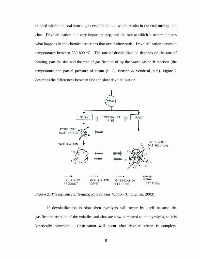
temperature and partial pressure of steam (S. A. Benson & Sondreal, n.d.). Figure 2

describes the differences between fast and slow devolatilization.

Figure 2: The influence of Heating Rate on Gasification.(C. Higman, 2003)

If devolatilization is slow then pyrolysis will occur by itself because the

gasification reaction of the volatiles and char are slow compared to the pyrolysis, so it is

kinetically controlled. Gasification will occur after devolatilization is complete.

9

However if devolatilization is fast pyrolysis and gasification will occur at the same time

because there was not enough time for the volatile matter to build up so that pyrolysis can

occur on its own. When coal is devolatilized it produces an array of different products

that include: tars, hydrocarbon liquid, and gasses like methane, carbon monoxide, carbon

dioxide, hydrogen, water and hydrogen cyanide. These products react with the oxygen in

the environment; the degree to which the products react with the oxygen depends on how

much volatile matter is produced (C. Higman, 2003). The reactions that govern the

overall conversion rate are the slowest reactions, these are: the Boudouard reaction, and

the hydrogenation reactions. Equally important, there are some physical steps that affect

the rate of reaction within a reactor. There are three temperature zones in the reactor a

low temperature, medium temperature and a high temperature zone that affect the

reaction rate, which is illustrated in Figure 3.

Figure 3: Reaction Rates in Temperature Zones.(C. Higman, 2003)

10

In the low temperature zone, the chemical reaction is the rate controlling step. In zone

two, although the rate of the chemical reaction is higher the reaction is limited by internal

diffusion of the reactants. Meanwhile, in the high temperature zone, the bulk surface

diffusion is the rate limiting step.

2.3 Types of reactors

According to Berkowitz’s definition of gasification only coal rank and temperature

affect the rate of gasification, and is better understood when looking at the different ways

to gasify coal. There are different reactor regimes that can be used to gasify coal, all of

which have characteristics that are unique to that process. The type of reactor that is

chosen for gasification will dictate what the operating conditions will be (temperature and

pressure) as well as what type of coal that can be used. There are three main types of

gasifiers that are in use today, they are the entrained flow gasifier, the moving bed

gasifier, and the fluidized bed gasifier. There are two more types of reactors that are not

as well known the transport reactor, which is similar to a fluidized bed and a torbed

reactor.

2.3.1 Entrained flow gasifier

In entrained-flow gasifiers, air or oxygen with steam is fed into the top of the

gasifier which causes the coal particles to become entrained within the reactor. In order

for this entrainment to occur the coal must be ground to a fine particle size of 100μm, this

fine particle size also ensures good mass transfer between the coal particles and oxidant.

Entrained flow gasifiers operate in a co-current flow pattern, and usually residence times

for these types of reactors are on the order of a few seconds. Entrained flow gasifiers

operate at high temperatures to ensure good conversion of carbon materials to syngas.

11

Also, operating at high temperatures ensure that all the ash is melted into slag, as a result

these reactor all operate in a slagging mode (“Impurities in Combustion and Gasification

Systems Lecture # 14 – Section 2 . Fireside behavior I – Transport Mechanisms Section 3

-- Fireside behavior of fuel impurities – slagging and fouling,” n.d.). The main advantage

to entrained-flow gasifiers is that they have the ability to handle any coal feedstock and

produce a clean, tar-free, syngas. Although the reactor is versatile in the type of coal that

is used certain coals are avoided due to the properties of the coal. For example, lignite

coal is often not desired for entrained flow gasifiers because of its high moisture content,

this requires more energy to be put into the reactor to evaporate the excess moisture and

is not as economical as the high ranked coals. Coals with high ash contents are also not

preferred because of the additional energy required to melt the ash into slag (R. E. .

Barrett, n.d.). The fine coal feed can be fed to the gasifier in either a dry or slurry form.

The slurry feed is a simpler operation, but it introduces water into the reactor which needs

to be evaporated. The result of this additional water is a product syngas with higher H2 to

CO ratio, but with a lower gasifier thermal efficiency. Entrained-flow gasifiers have a

high conversion efficiency of 98% of converting material into syngas. This key trait is

why entrained flow gasifiers are used in practice in such technologies as Integrated

Combined Gas Cycle (IGCC) and thus the technology for this type of reactor is the most

developed. One major drawback to this reactor type is that it requires a lot of oxidant to

get a good conversion which increases the operating cost of the reactor. An example of

an entrained-flow gasifier can be seen in Figure 4. Figure 4 is a picture of Texaco’s

entrained-flow gasifier which has heat exchanger tubes inside the reactor.

12

Figure 4: Texaco’s Entrained Flow Gasifier (“NETL.doe.gov,” n.d.)

2.3.2 Moving bed gasifier

In a moving bed gasifier, large particles move down the reactor, and reacts with

gasses that are moving countercurrent to the coal particles. The particle size of the coal

for this reactor should be course so that there is good permeability within the particle.

Also, the courser the particle size the less chance of chemical burning and less of a

pressure drop through the reactor. Reactions in this reactor take place in different zones

of the reactor. The top of the gasifier is considered the drying zone. The coal enters the

reactor here and is heated and dried by the product gas leaving the reactor. Meanwhile,

the products gas is interacting with the fresh feed and as a result is cooled upon making

its exit out the reactor. The coal then makes its way to what is known as the

13

carbonization zone. This is where devolatilization and pyrolysis occur. Next is the

gasification zone, where the char reacts with steam and carbon dioxide. Finally at the

bottom of the reactor is where the combustion zone is. This zone is where oxygen reacts

with the char it is the hottest zone due to the fact that the combustion reactions are

exothermic. The Moving Bed gasifier can operate in two different modes, a dry ash

mode and in a slagging mode. In dry ash mode, the temperature is controlled with steam

and the gasifier is operated at a temperature below the ash-slagging temperature, Figure

5.

Figure 5: Bed Gasifier operating in Dry-Ash Mode (“NETL.doe.gov,” n.d.)

The excess steam reacts with the char and prevents the formation of ash. There is

excess ash is still produced in the combustion zone of the reactor, which is cooled by the

excess steam, which promotes solidification of the ash that is produced. An example of

an entrained flow gasifier, which operates in dry ash mode, is the Lurgi dry ash gasifier.

In slagging mode operation, less steam is used, which results in a higher operating

14

temperature. This higher temperature allows for the ash to melt and form slag within the

reactor. An example of a moving bed gasifier that operates in slagging mode is the BGL

gasifier. Moving bed reactors can handle low ranked coals that exhibit high reactivity’s

(R. E. Barrett, n.d.) such as lignite. In fact, if higher ranked coals are going to be used

then the design of the reactor has to modify in order to account for the swelling and

caking those higher ranked coals, such as bituminous coal exhibits. One main advantage

to utilizing this type of gasifier is that it does not require a large amount of oxidant for

operation, which lowers the operating cost of the process. Equally important, there is less

preparation of the feedstock going into the reactor. Larger particle sizes of coal can be

used, and thus eliminates the need to grind the coal to a particular mesh size. The

moving bed gasifier has some disadvantages as well, one of which is it has a hard time

handling the fine particulate matter produced in the coal ash. Another disadvantage is that

tars are produced in the reactor which can cause problems with limiting heat and mass

transfer.

Although there is a third gasification system, the paper will now switch gears to

discuss lignite as a fuel source and the associated problems with it. Then go back to

explaining the last gasification system and then tie the use of lignite as a fuel source into

fluidized bed gasifiers.

2.3.3 Fluidized bed reactor

Fluidized-bed gasifiers employ a reactor bed contained with a fluidizing, solid,

medium such as sand. Coal is fed into the side of the reactor, while the oxidant (air or

oxygen) are fed in from the bottom to promote the fluidizing of the sand. Once the sand

is fluidized it takes on properties that act more like a fluid then a solid. Fluidized beds

15

promote back-mixing, and efficiently mix feed coal particles with coal particles already

undergoing gasification see Figure 6.

Figure 6: Depiction of a fluidized bed.(“NETL.doe.gov,” n.d.)

Due to the thorough mixing within the gasifier, a constant temperature is sustained in the

reactor bed. In fluidized reactor regimes, the operating temperature should be high

enough to decompose the tars and other liquid products produced during pyrolysis and

devolatilization. At the same time the temperature is should be lower than the softening

point of ash. This is to prevent ash from being formed, because ash can cause problems

such as defluidization as well as inhibit heat and mass transfer. Due to this temperature

constraints highly reactive coals, such as lignite are often utilized so that a good carbon

conversion can be achieved at the lower operating temperatures. During Fluidization

some char particles are entrained in the raw syngas as its leaves the top of the gasifier,

16

but are recovered and recycled back to the reactor via a cyclone. Ash particles, removed

below the bed, give up heat to the incoming steam and recycle gas. At startup, the bed is

heated externally before the feedstock is introduced. To sustain fluidization, or

suspension of coal particles within the gasifier, coal of small particles sizes (<6 mm) is

normally used.

2.4 Fuel quality and fuel properties

Coal forms from a natural process that occurs over time. It involves plant life

absorbing carbon dioxide from the atmosphere. A combination of sunlight, moisture,

temperature, pressure and time; the carbon dioxide from the plants get converted into

compounds such as carbon, oxygen, hydrogen as well as complex substances like sugars,

starches cellulose and lignin (Raask, 1985). Over time, this vegetation is converted into

various forms of coal. The organic matter will first turn into peat, which is a woody

substance. The peat gets buried it becomes compressed and secluded from oxygen which

is the first step in the transformation of peat into coal.

Coals are classified by rank, with lignite being the lowest ranked coal, then sub-

bituminous, bituminous and anthracite the highest. The most widely accepted method to

classify coal is the ASTM method. This method classifies coal based on the amount of

fixed carbon, and heating value, which is calculated in a mineral matter free basis. There

are some common trends that occur with coal properties as coal climbs higher in rank.

Generally since lower ranked coals are younger coals, they contain higher moisture

content, a lower heating value along with a lower amount of fixed carbon. Equally

important, as the rank of coal increases the amount of oxygen decreases, which gives

important insight to the characteristics of the coal. The amount of oxygen in the coal is an

17

indication of how reactive the coal is, this reactivity has an influence on operating

conditions and the type of reactor which will be best suited for that type of coal, which

will be discussed later. It can be seen from Figure 7 the chemical and physical

compositions of coals according to rank. It is also important to not from the table that the

percent of volatile matter within the coal also decreases with increasing coal rank.

Figure 7: Chemical and Physical Properties of Coals in the Various Rank Classes (S.

Benson, n.d.; Description, n.d.)

Impurities are an important and unique characteristic of coal they appear in

different forms of mineral matter that are present in the coal. Coal can have up to fifty to

sixty different types of minerals, however the major ones include clay, sulfides, sulfates,

carbonates and silicates. Impurities are important because they impact the design,

performance, and reliability of the system. Impurities also cause pollution and can be

toxic. Impurities are associated in coal by different means. Impurities can be water

associated, with water soluble minerals. These types of associations are in small

18

amounts. Impurities can also be associated in mineral grains, which can either be

included or excluded in the coal particle. Finally there are organically associated

impurities. These impurities are bound as salts of carboxylic acid, along with organically

associated sulfur. Impurities in coal are rank dependent, that is in high ranked coals such

as anthracite and bituminous the impurities are primarily mineral associated whereas the

low ranked coals the impurities are organically associated, water associated and mineral

associated. Organically associated impurities, prove to cause the most trouble in

combustion/gasification systems. This is due to the fact that, these impurities are released

when the coal is heated up, and can cause corrosion and fouling problems to equipment.

Since lignite contains a lot of volatile matter, there are a lot more impurities organically

associated with it compared to a higher ranked coal. This, along with Lignite’s high

moisture content, makes it a challenging fuel to utilize for combustion and gasification

systems.

2.4.1 Lignite coal

Low rank coal such as lignite and subbituminous coals are in large abundance

throughout the world. According to the U.S Department of energy, the world contains

514 billion metric tons of low rank reserves. In the United States alone contains

approximately 149 million tons of low rank coal reserves. Utilizing these reserves for

practical purposes can alleviate the United States dependence on foreign Oil and help the

country become energy independent. However using low rank coals such as lignite,

present challenges in gasification systems. If these challenges can be overcome, then the

use of lignite for gasification can provide many opportunities for gasification

applications. Some of the challenges that lignite presents in gasification systems are high

19

moisture content, high reactivity, non-caking properties, ash content, and inorganic

material such as sodium.

The reactions of lignite coals in gasification systems are unique to the properties

that the fuel posses, that make them different than bituminous coals. Due to the unique

properties of lignite, technologies that have been used for bituminous coal applications

must be modified in order for them to be used on lignite. Specifically, when compared to

bituminous coals lignites have a different molecular and physical structure, a significantly

higher moisture content, lower heating value, higher porosity and surface area and

different mineral content. These are important factors that influence and dictate how

lignite will be utilized when being applied to different gasification systems.

High moisture content has an effect on the operating conditions of the gasifier, the

feeding system requirements, and the process yields of the product gas. High moisture

content also means it can reduce the energy density of the coal; this is mainly why lignite

coals have a lower heating value then bituminous and subbituminous coals. Data has been

collected by studies that show that North Dakota lignites normally have moisture contents

of 35% and above. Moisture in low rank coals is present in the coal due to hydrogen

bonding both on the surface of the coal, as well as in the pores within the coal. The

hydrogen bonding in the coal helps contribute to the rigid structure that characterizes

lignites. Which helps explain why when lignite is dried, the structure becomes greatly

weakened.

Lignites are known to have high sodium content in the ash that is produced. This

mineral matter can cause corrosion problems in high temperature applications. At high

temperatures the sodium vaporizes and becomes a part of the syngas. After the

20

gasification process the syngas will go through unit operations such as heat exchangers or

boilers (depending on the application), where the temperature of the gas will decrease.

As a result of this temperature decrease (in the case of syngas cooling) the sodium will

condense onto the heat transfer surfaces. This will cause fouling and corrosion, and will

decrease the efficiency of the heat exchanger. The high amounts of carboxylic groups

influence the behavior of alkali metals such as sodium. It is proposed that when the

carboxylic acids start to decompose at low temperatures that mechanism plays a

significant role in the sodium that is contained within the carboxylic acid. The sodium

gets released into the ash which can cause the fouling of equipment. During gasification

there are many different chemical transformations occurring simultaneously that

influence the ash formation. These phases are aluminosilicate, silicate, sulfides, and

metals. Sodium is known to react with all of these phases. And generally sodium has

been found to take these various forms within the ash composition: Na2O, NaOH, Na2S,

sodium silicates and sodium aluminosilicates (Raask, 1985).

Each type of fuel can have specific problems related to the mineral matter in

boiler operation. Ash analysis taken from O’Gorman and Walker (1972) showed that

gypsum, pyrite, and thenardite (sodium sulfate) were the principle constituents of the low

temperature ash. Sodium sulfate can form at low temperatures when coal is heated in an

oxidizing environment with its mineral matter. Alkali metals, such as sodium, are within

the coal matrix in different forms such as organometal salts, chlorides, sulfates,

carbonates, and silicates. One explanation as to why lignites, especially lignites from

North Dakota, contain large amounts of sodium is due to the local ground water. The

ground water contains a lot of sodium, and because coal has a very porous structure,

21

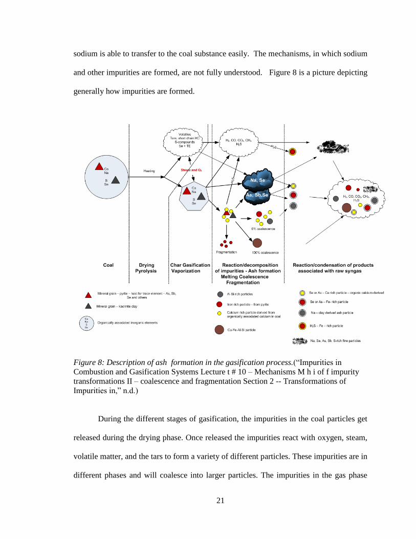
sodium is able to transfer to the coal substance easily. The mechanisms, in which sodium

and other impurities are formed, are not fully understood. Figure 8 is a picture depicting

generally how impurities are formed.

Figure 8: Description of ash formation in the gasification process.(“Impurities in

Combustion and Gasification Systems Lecture t # 10 – Mechanisms M h i of f impurity

transformations II – coalescence and fragmentation Section 2 -- Transformations of

Impurities in,” n.d.)

During the different stages of gasification, the impurities in the coal particles get

released during the drying phase. Once released the impurities react with oxygen, steam,

volatile matter, and the tars to form a variety of different particles. These impurities are in

different phases and will coalesce into larger particles. The impurities in the gas phase

22

will condense, and the impurities in the liquid phase will solidify, which will cause

problems to equipment downstream of the gasification process such as boilers and syngas

coolers. Research has shown that salts such as sodium chloride do not volatilize below

475 K, on its own. However, some researchers have shown through experiments that

sodium chloride does form eutectoids with other minerals in the ash.

Lignite is a highly reactive coal in reducing Environments, but the reactivity does

not correlate with the surface area (Timpe et el 1989). However, the high reactivity of

low ranked coals can be attributed to the abundance of free radicals that are formed

during thermal transformations of oxygen functional groups. An example of such a

mechanism is decarboxylation. The free radicals can either react with volatile species or

coalesce to form a highly cross linked solid char. This newly formed char is what gives

low ranked coals their non-caking characteristic. Due to the fact that this cross linked

char is non-caking, allows for more mixing and reaction at higher temperature. This

cross linking phenomena that occurs in lignites during gasification differs than what

bituminous coals undergo when gasified. When a bituminous coal is gasified, the char

melts which forms a liquid in the coal, known as tar. This is because the micro-porous

structure of lignite is enlarged as carbon is consumed which increases diffusion across a

more open structure. As a result, the reactivity’s of low ranked coals at lower

temperatures are much higher than bituminous coals. The higher reactivity is influenced

by the larger pore structure, and the catalytic affect of organically associated cations such

as calcium, magnesium and sodium. One of the positive attributes of utilizing lignite as a

fuel source is that it the coal will form less tars than its bituminous counterpart which can

prevent problems like plugging up the reactor.

23

2.5 Impurity transformations

The impurities in lignite are released during the gasification of coal. The impurities

that cause a lot of the problems are iron, sulfur, sodium and potassium. These impurities

affect the performance of gasification reactors. Depending on the type of reactor will

depend on how they affect the gasification process. With a high temperature reactor the

impurities will released. The more volatile species will travel through the process and

condense on heat transfer surfaces. This condensation will cause corrosion and wear on

these heat transfer surfaces and decrease efficiencies. Meanwhile the less volatile species

will attached themselves to the reactor walls and create a viscous, molten slag. This slag

can build up and cause physical damage as well as an increase in operating temperature

to achieve the same quality of gasification. Figure 9 is a schematic of ash deposition build

up on the inside of a reactor wall. In a high temperature reactor, such as an entrained

flow reactor, the impurities will have the same effect as in a high temperature boiler. The

rate of fouling and slagging depends on the temperature of the deposit collecting surface

and on the temperature gradient across the deposit layer.

24

Figure 9: Impurity buildup of slag and temperature profile between the

furnace and slag layer

Once the impurities are released from the coal they start to deposit onto the wall and

condense based on their boiling point. Starting right after steam in figure 4, going from

left to right the dark, black region, are metal deposits, followed by alkali salts, silicates +

salts and then silicates. Metals deposit is usually due to the combustion of pyrite rich

coals. The layering affect is due to the temperature gradient across the deposits. The

temperature gets hotter as it enters different regions of the slag, and is hottest in the flue

gas. These temperature differences influence different minerals in the coal and how they

condense on to the surface. As these layers build different minerals will form their own

unique slag layer accordingly. In low temperature reactors such as fluidized bed reactors,

the impurities affect the gasification in a different way. Since fluidized beds operate at a

temperature that is below the softening point of ash, slagging is not a problem like in the

high temperature reactors. This is not to say that fluidized beds do not have their own

problems. Since fluidized bed reactors operate at lower temperatures, lower ranked coals

25

are used because they are more reactive, which makes up for that lower operating

temperature. A major problem in low temperature fluidized bed reactors is agglomeration

of bed material, which results in defluidization of the reactor. This results in reactor

being offline, for repair which can cause loss in profits. Agglomeration in fluidized beds

occurs due to the high sodium content in lignite. Lignite, like most coals contain a lot of

clays, and pyrite. The high sodium in the lignite gets released and reacts with silica,

which is a common bed material in fluidized bed to form low temperature eutectics. The

sulfur is released from the pyrite and acts as a binding agent between the sodium and the

silica, the result is agglomeration. Typically fluidized beds operate in the range of 850 °C

to 950 °C. However, agglomeration typically begins at temperatures lower than the

operating temperature.. Impurities affect both high temperatures as well as low

temperature reactors. In low temperature reactors there is a more immediate effect on

process, which can result in immediate shutdown due to agglomeration. Whereas in high

temperature reactors impurities have a more of a delayed affect causing damaging

corrosion and slag affects over time.

2.6 Impacts of impurities

Impurities have a large impact on gasification process. The fuel properties of

lignite have to be considered in the design and operation of reactors. The influence of the

impurities in the ash requires larger design surface areas, and operational costs. A major

influence on impurities is the temperature. Impurities will behave at different

temperatures. Equally important the mode of occurrence will also influence the impact

impurities have on the gasification process. Lignite has a large amount of volatile matter

with inorganic minerals organically associated within the coal matrix. The impurities

26

will affect both high temperature reactors as well as low temperature reactors. It’s the

same problem, but affects both situations in a unique way. With high temperature

reactors the impurities will cause slagging, corrosion and fouling on equipment. In low

temperature reactors, the impurities cause agglomeration, and corrosion on heat transfer

surfaces.

2.7 Measures to minimize impurities

2.7.1 Alternative bed materials

Since silica sand is the primary cause of agglomeration by reacting with sodium,

as well as the primary bed material, using a different bed material would cause less or no

agglomeration. Alumina and alumina sand was investigated (Bartels, Lin, Nijenhuis,

Kapteijn, & van Ommen, 2008). It was shown that whereas with silica agglomeration

started to occur at temperatures as low as 700 degrees C with an alumina bed

agglomeration did not start until 800 degree C. the application of alumina sand was

investigated in a fluidized bed of straw pellets and the results were that agglomeration

started at 920 degrees C. the results of these experiments showed that alumina allows for

an increase in operating temperature will prevent agglomeration from occurring so

quickly (Bartels). Other bed material to replace the typical silica sand bed include:

Mullite Sand (2SiO2 3Al2O3), Sillimanite (Al2SiO5), Magnesium Oxide (MgO),

Magnesite (MgCO3), Limestone (CaCO3), Dolomite (CaMg(CO3)2), Ferric Oxide

(Fe2O3), pre-calcined Dolomite, Bauxite (high in Al), and zirconium sand (ZrSiO4). All

of this material showed an improvement to the prevention of agglomeration. It should be

noted that magnesium oxide agglomeration mechanisms are different than that of silica.

Equally important, abrasion and erosion was an issue with the pre-calcined dolomite.

27

2.7.2 Mineral additives

In order to limit the low melting point eutectics from forming, one proposed

solution is to add minerals to the fluidized bed. These minerals will alter the ash

characteristics that are deposited on the bed particles. The additives react with alkalis to

form higher melting point eutectics. These mineral additives include, clay, kaosil, and

bauxite to help limit agglomeration in silica sand based bed.

2.7.3 Pre-treating coals

Pre-treating the coal involves removal of sodium by water washing the coal

before gasification. Alternatively, another avenue is to add aluminum or calcium to the

coal before gasification. This will change the ash characteristics from a low melting point

ash to a higher melting point ash (Zhang, D Jackson, P Vuthaluru, n.d.) . Pre-treating the

coal with aluminum showed the coal ash was high in Al-rich phases of high melting

points.

2.7.4 Blending of coals

This method involves blending high sodium/high sulfur lignite with a sub-

bituminous coal that has higher ash content, with lower sodium and sulfur. The idea

behind this is that the high melting point ash of the subbituminous enriches the coal with

high melting point ash and reduces the low melting point ash species (Zhang, D Jackson,

P Vuthaluru, n.d.). Research from Vuthaluru showed that irrespective of the blend ratio,

the results showed that aluminum retention in the bed ash and fly ash was higher than the

raw coal runs. This is due to the fact that there are higher levels of aluminum in the sub-

bituminous samples. Edax analysis showed in several regions the presence of sulfated ash

28

dissolved in high melting Al/Si/Mg/Ca-rich ash. These high melting phases were also

confirmed by XRD analysis, by the same researches

2.8 Applications

Gasification is a technology that can be very useful in the future to meet many of

the worlds needs. This is because that gasification is a process that produces a syngas

that can be used for many different applications. The three main applications of

gasification are the production of chemicals, synfuels and electricity (“The Future of

Coal-Options for a Carbon-Constrained World,” n.d.). Figure 10 depicts the gasification

process with its ability to use different feed-stocks to produce many different products.

Figure 10: Schematic of Applications for gasification3

It can be seen from Figure 4 that a large variety of chemicals can be produced.

Among these are Ammonia, Methanol and Hydrogen.

29

2.8.1 Fuel Production

2.8.1.1 Methane

Methane is produced from with the use of a nickel catalyst, directly from the

syngas. Methane production usually occurs at lower temperatures between

700 °C to 1000 °C. These lower temperatures makes fluidized bed technology

suitable for methane production, because the operating temperatures operate

in the same range. The organically associated sodium and calcium found in

lignite, which are usually associated with problems provide catalytic activity

for methane production (Benson and Sondreal, 2010). The methane reaction

is exothermic. Examples in industry where gasification syngas is used to

produced methane were in North Dakota DGC’s GPSP operated on high-

sodium lignite (S. A. Benson & Sondreal, n.d.) Methanol

Approximately 9% of the world’s methanol production is based on coal

gasification (Chmielniak & Sciazko, 2003). Most methanol gasification plants are

smaller than traditional plants. Methanol synthesis reactions take place when carbon

monoxide and carbon dioxide react with hydrogen to produce methanol and water, in

which both reactions are exothermic. The process is catalytic and uses a copper-zinc

catalyst. Some design considerations for methanol include gasification pressure, syngas

cooling arrangement, and acid-gas removal. Methanol can be used to for energy, fuel

such as gasoline, fuel cells and act as a building block for synthetic hydrocarbons.

2.8.1.2 Fischer-Trospsch synthesis

The Fischer-Trospsch process is a large scale process that can produce liquid

fuels from syngas derived coal. The main components of the Fischer-

30

Trospsch process include alkanes, alkenes, and alcohols. This process uses a

heterogeneous catalytic process to produce liquid fuels. A gasification plant

in South Africa called Sasol utilizes Fischer-Trospsch synthesis to convert

coal derived syngas into liquid fuels.

2.8.2 Chemical Production

2.8.2.1 Ammonia

Over 90% of ammonia is produced by the reforming of natural gas; the rest is

produced by gasification of coal or oil. There are certain specifications associated with

the ammonia process like nitrogen to hydrogen ratio, the amount of water and the

combined amount of carbon monoxide and carbon dioxide must be below 30ppmv as

well as limitations on sulfur and inerts. Ammonia plants based on gasification

technologies normally surpass these specifications. Some of the design considerations

for an ammonia plant based on gasification are the removal of tars, desulfurization, CO2

removal, and adjustment of the nitrogen to hydrogen ratio.

2.8.3 Hydrogen Production

Hydrogen is traditionally largely produced by steam reforming of natural gas,

however, about 32% of the hydrogen produced in the world comes from gasification14

.

Early gasification systems were called retorts. They were externally heated systems

which were heated indirectly from the combustion gasses. Early on these systems were

used to produce town gas. In the 1940’s a retort system was used at the University of

North Dakota to convert lignite to a hydrogen rich stream. The gasifier used was a fixed

bed. Steam Hydrogen can typically be used for silicon wafer production and optic fiber

31

cable production. Some design considerations of hydrogen production through

gasification are the same as methanol.

2.8.4 Power generation

Power generation via gasification has received a lot of attention, especially in the

United States as part of the Clean Coal Power Initiative (“The Coal Resource- A

Comprehensive Overview of Coal,” 2005). The most well-known design for this purpose

is the integrated gasification combined cycle (IGCC) (Maurstad, Herzog, Bolland, &

Beér, n.d.). Power generation from gasification is predicted to be one of the dominant

markets for gasification technology with IGCC as the primary design. Due to increasing

environmental restrictions on the emissions of coal, IGCC technology provides a clean

way to continue to use coal as an energy resource. In an integrated combined gas cycle,

the syngas produced from gasification is used to drive a turbine to generate electricity.

Integration of the gasifier, gas turbine, and steam turbine allows for higher efficiencies

(Powell, C.; Morreale, 2008). Figure 11 compares the efficiencies for a typical low

ranked coal and a typical bituminous coal for different technologies including

conventional pulverized coal combustion to IGCC.

http://www.netl.doe.gov/technologies/coalpower/cctc/

32

Figure 11: Comparison of efficiencies for power generation of low and high

ranked coals (Zhang, D Jackson, P Vuthaluru, n.d.)

IGCC plants provide environmental benefits from traditional combustion applications.

IGCC plants are particularly well-suited for co-generation. An IGCC plant could produce

power when electricity prices are high, but scale back power production and divert

syngas to another product, like transportation fuels or chemicals. Some challenges of

IGCC include High Capital costs compared with alternative power plant designs,

financial viability is often dependent upon subsidies or tax credits (“NETL.doe.gov,”

n.d.). As a relatively new technology relative to Pulverized Coal the development and

design costs are much higher for IGCC. Availability also impacts operating costs and

must be consistent enough to meet growing electricity demand. The complexity of IGCC

33

relative to older, more established plant designs (Maurstad et al., n.d.), also increases

operating costs and can impact availability and the generation of capital for plant

development. Fluidized bed gasification can be the basis for new technologies from low

rank coal to achieve high overall process efficiency.

2.9 Summary

Gasification is an old technology that has the potential to provide the answers to a

more sustainable energy future. The applications of gasification technology are

numerous and diverse. Continuing to advance the research is imperative to overcome

some of the challenges the prevent gasification technology to gain more mainstream

success. Fluidized bed gasification is the least developed, however provides

advantages in utilizing lignite coal, an abundant resource in the United States.

34

Chapter III

3. DETAILED DESIGN OF A FLUIDIZED BED AND ITS ASSOCIATED UNIT

OPERATIONS FOR COAL COMBUSTION AND GASIFICATION

3.1 Introduction

Of the three main types of gasification reactors mentioned in the literature, the fluidized

bed is the least utilized in industry. This could be due to the challenges associated with fluidized

beds such as difficulty in scaling-up from a bench scale reactor(Pugsley, T. Mahinpey, n.d.).

Another possibility is that when using low-ranked fuels, such as lignite, it creates problems with

the fluidization, which is difficult to control. Despite these challenges, there are fluidized beds

being used in industry for gasification applications. Currently there are six types of gasification

processes using fluidized bed gasifiers operated at an industrial scale (Collot, 2006). These

technologies include: the BHEL fluidized bed gasifier, the High Temperature Winkler (HTW)

gasifier, the Integrated Drying Gasification Combined Cycle (IDGC), the Kellogg Rust

Westinghouse (KWR) gasifier or U-gas, the Kellogg Brown and Root (KBR) Transport gasifier,

and Great Point Energy. Of these six technologies the KBR and IDGCC gasifiers are circulating

fluidized beds, (CFB), while the rest are bubbling fluidized beds, (BFB). Between these six

technologies, three of them are used exclusively for power generation (KBR, HTW, and

IDGCC). While only one is used exclusively for the production of synthetic natural gas, (Great

Point Energy). Meanwhile the other two, KBR and U-gas produce a syngas that has the capacity

for power generation, production of chemical or fuels. Fluidized bed technology is an attractive

way to gasify coal. There are many advantages to using fluidized beds for gasification

compared to Entrained Flow and Moving Bed gasification reactor technologies. The fluidized

bed reactor consists of a reactor that contains a fluidizing medium. Typically the fluidizing

medium is sand; however research has been done with other bed materials. The selection of bed

35

material will largely depend on the application, along with the fuel type in the reactor. The

fluidizing medium exploits one of the most attractive features of a fluidized which is its ability to

maintain a uniform temperature throughout the bed. Equally important, the mixing of sand

promotes good heat and mass transfer which result in the chemical reactions getting carried out

closer to completion. For combustion applications, the fluidized bed also offers some

advantages over traditional combustion furnace regimes. The fluidized bed for combustion

offers a better way to control and mitigate pollution from the production of SOx and NOx. In a

fluidized bed, Combustion takes place at lower temperatures of 760 °C to 982 °C compared to

conventional combustion systems, where combustion takes place between 1398 °C to 1899 °C

(S. A. Benson, 1985). The lower operating temperature of the bed allows for the ability to use

lower quality fuels, and in the case where there are in bed tubes, the lower temperature reduces

tube fouling. Lastly, due to the thorough mixing, the heat transfer in a fluidized bed is five times

greater than the convective section of a typical combustion system which will result in a

reduction in overall combustor size (S. A. Benson, 1985). The size and density of particles

affects the operating behavior of the fluidized bed. Geldart proposed a classification system for

particles that share similar characteristics into four different groups. These groups are based on

the solid-fluid density difference and particle size. The design of a fluidized bed can based on

which Geldart particle group is selected, which will dictate which fluidization regime and what

type of fluidized bed will be used. The four different groups in the Geldart classification system

are group A, group B, group C, and group D. Group A particles range in size from 20 to 100 μm,

with densities less than 1.4g/cm3 and are used mainly in powder catalyzed beds. Particles in

group B have a particle size range of 40 to 500 μm with densities between 1.4 and 4 g/cm3; these

are described as sand-like particles. Group C has size range of 20 to 30 μm, they are fine and

36

cohesive and can be difficult to fluidize, without mechanical agitation. Group D are larger

particles with a size of 600 μm and above. High fluid velocities are required to fluidize these

particles, which have high densities and can cause abrasion. A fluidized bed uses air and in

gasification applications, steam to both act as the fluidizing medium as well as the vehicle to

react with the coal and carry out the combustion or gasification process. The air enters in from

the bottom of the reactor, through a distributor plate. As the air moves through the bed the

pressure builds up to a certain point. In this stage it is considered a packed bed. Once the

velocity exceeds a value the pressure drop remains constant, and is equal to the weight of the

bed, at this point the particles in the bed are moving and the reactor is considered a fluidized bed.

A characteristic of the fluidized bed is that it exhibits two phase flow, which can be difficult to

characterize and fully understand. Along with this complex, two phase phenomena; kinetic data

is not readily available. This is in part, why there is no straight forward method to design a

fluidized bed. As a result, fluidized bed design is based largely on empirical equations, along

with the designers overall experience with gasification. The following work will present the

detailed design of a fluidized bed reactor for combustion and gasification, along with the unit

operations that are associated for the gasification process. The Focus of the work was to design a

small scale fluidized bed, because of this, that is where most of the detail and emphasis has been

placed. An attempt has been made to present this design in clear straight forward manner;

however, there is not one specific way to design a fluidized bed.

3.2 Fluidized bed design

3.2.1 Fluidization Calculations

A Fluidized bed gasifier was designed based fluidization calculations, and combustion

calculations taken from the literature. The reactor was designed using lignite coal as the design

37

fuel. There are many different unit operations that are required to make a fluidized bed process

operate. These unit operations include a fuel feeding system, an air pre-heater, a cyclone, and

two condensers to remove any liquids from the syngas, see Figure 12.

Figure 12: Process flow diagram of the gasification process.

From Figure 12 air and steam will be fed into the reactor from the bottom, and mix before going

through the distributor plate. Coal will be fed into the reactor from the side, and the reaction will

take place within the fluidized sand bed. Once the gasification reactions take place, the syngas

will be cleaned up by going through a pollution control cleanup system. This system will consist

of a cyclone, which will remove the any particulate matter in the syngas, as well as any bed

material that may be elutriated. Next, the syngas will go through a pair of condensers. These

condensers will remove and condensable organic material, such as tar, as well as water. The

fluidized bed will be controlled through pressure gauges. This will allow the operator insight to

how to fluidized bed is behaving, by monitoring the pressure the type of fluidizing regime will

be known, as well as if there are any problems occurring such as agglomeration formation, which

38

may cause fluidization to decrease or stop all together. Next, the temperature will be monitored

at different points of the process, for safety purposes. The reactor’s temperature will be

monitored, as well as, at different locations downstream, which will also serve as a way to

regulate and condense out any organic tar like, and aqueous material. Figure 12 describes the

overall gasification process, but inside the reactor is where the coal, air and steam enter and the

gasification reactions take place. As the gas flowrate through the fixed bed is increased, the

pressure drop will rise until the minimum fluidization velocity is reached, the packed bed will

then become fluidized. The onset of fluidization occurs when the drag force of the upward

moving gas equals the weight of the particles, in this state, the sand particles takes on the

behavior of a fluid. When the gas flowrate is further increased, the fluidized bed will go through

different fluidizing regimes. For Geldart group B particles an increase in the gas flowrate will

change the fluidization regime from a bubbling bed, to a slugging bed or turbulent churning , and

with a further increase in velocity, into the fast fluidization regime and pneumatic transport. At

the point of fast fluidization, the bed material will be blown out and will need to be recycled and

replenished with new bed material. The key advantage to a fluidized is bed is the fluidizing of

solid particles so that they take on the characteristics of a fluid rather than a solid, this mixing

allows for a uniform bed temperature as well as enhancing the heat and mass transfer. It is the

heat and mass transfer enable the gasification reactions to take place. As a result the heat and

mass transfer, and therefore the gasification reactions are heavily dependent on the fluidization

parameters. Because of this, the design of the fluidized bed focuses and emphasizes the

fluidization calculations first and, the combustion calculations as secondary. the following

section will explain the different fluidization parameters and calculations and how they influence

the design of the reactor, starting with the minimum fluidization velocity.

39

3.2.1.1 Minimum Fluidization velocity

The minimum fluidization velocity is one of, if not the most, important design parameters

for fluidized beds; and is largely determined by both the size of the particles in the bed, as well

as the bulk density of the particles. To a lesser extent, the minimum fluidization is also

influenced on operating conditions such as temperature and pressure. For this calculation the

particles in the bed are taken as sand and the fluidizing medium is a mixture of air and steam, but

since air is present in a much larger quantity in steam, only air will be considered in the

calculation. Sand is considered a Geldart B particle. The steam is neglected for ease of

calculation. The properties of air were determined for the operating conditions of 1500 degrees

Fahrenheit and at atmospheric pressure. The minimum fluidization was calculated based on an

average particle size of 595 microns. It is important to base the minimum fluidization velocity

on the average particle size of the bed oppose to a uniform particle size because it will provide a

better representation of particles that are actually in the bed. Equally important, bed material can

be lost during operation due to the elutriation of particles, which requires replenishing the bed

material during operation. These bed materials can vary in size from the particles are actually in

the bed. Based on the design methods presented by Kunii and Levenspiel in Fluidization

Engineering 2nd

Edition, the minimum fluidization velocity was calculated using the formula:

(Eq: 3.1)

Where

Umf= Minimum fluidization velocity of the particles within the bed.

dp is the diameter of the particle,

ρs and ρg are the densities of the particle and fluid respectively,

g is the acceleration due to gravity,

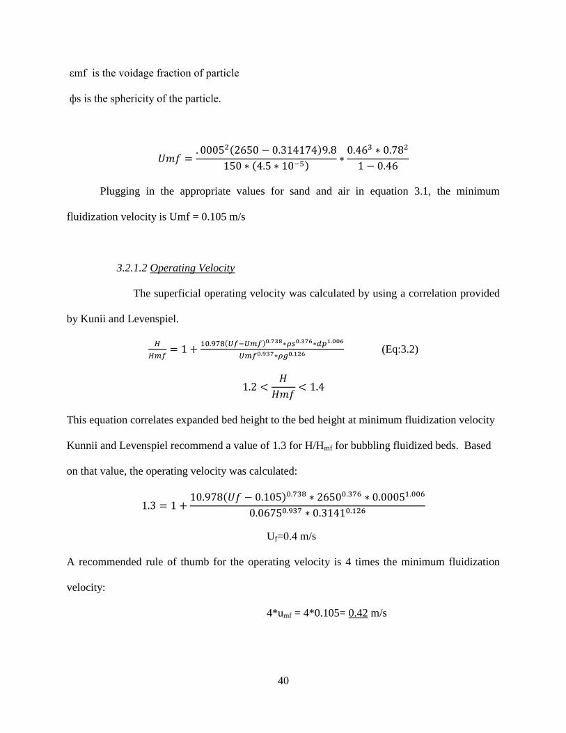
40

εmf is the voidage fraction of particle

фs is the sphericity of the particle.

Plugging in the appropriate values for sand and air in equation 3.1, the minimum

fluidization velocity is Umf = 0.105 m/s

3.2.1.2 Operating Velocity

The superficial operating velocity was calculated by using a correlation provided

by Kunii and Levenspiel.

(Eq:3.2)

This equation correlates expanded bed height to the bed height at minimum fluidization velocity

Kunnii and Levenspiel recommend a value of 1.3 for H/Hmf for bubbling fluidized beds. Based

on that value, the operating velocity was calculated:

Uf=0.4 m/s

A recommended rule of thumb for the operating velocity is 4 times the minimum fluidization

velocity:

4*umf = 4*0.105= 0.42 m/s

41

This value is recommended to ensure good quality fluidization. The value calculated from

equation 3.2 is in close agreement with the rule of thumb. The rule of thumb acts as a check to

make sure the operating velocity is within a reasonable range to ensure good fluidization.

3.2.1.3 Characterizing the fluidization in the reactor

Now that the operating velocity has been calculated, it can be used in conjunction with the

average particle size in the bed to map out the fluidizing regime of the reactor. This will identify

the range and characterize what type fluidization will be occurring (i.e.: bubbling, fast, or

pneumatic transport). In order to map out the fluidization regime, two dimensionless quantities

are calculated and .

(Eq: 3.3)

(Eq: 3.4)

Once calculated, these values can be plotted against a fluid mapping chart, provided by Kunii

and Levenspiel to predict which fluidization regime the reactor will behave like at operating

conditions. Plugging in the values at operating conditions for (Eq: 3.3) and (Eq:3.4):

=0.18

=7.9

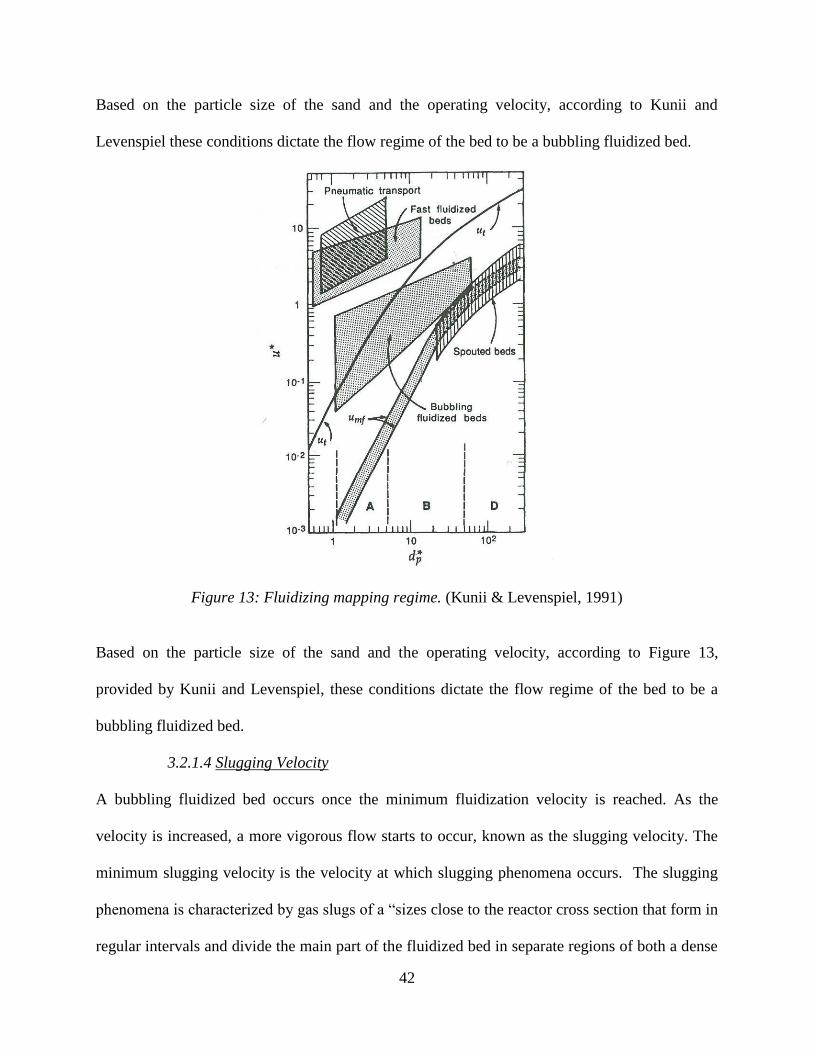
42

Based on the particle size of the sand and the operating velocity, according to Kunii and

Levenspiel these conditions dictate the flow regime of the bed to be a bubbling fluidized bed.

Figure 13: Fluidizing mapping regime. (Kunii & Levenspiel, 1991)

Based on the particle size of the sand and the operating velocity, according to Figure 13,

provided by Kunii and Levenspiel, these conditions dictate the flow regime of the bed to be a

bubbling fluidized bed.

3.2.1.4 Slugging Velocity

A bubbling fluidized bed occurs once the minimum fluidization velocity is reached. As the

velocity is increased, a more vigorous flow starts to occur, known as the slugging velocity. The

minimum slugging velocity is the velocity at which slugging phenomena occurs. The slugging

phenomena is characterized by gas slugs of a “sizes close to the reactor cross section that form in

regular intervals and divide the main part of the fluidized bed in separate regions of both a dense

43

and a lean phase (Wen-Ching Yang, 2003).” Slugging regimes can occur in deep beds which is

defined as a bed with an aspect ratio that is greater than one, but usually occurs with an aspect

ratio that is greater than 2 (Rao, Curtis, Hancock, & Wassgren, 2010). The aspect ratio is

defined as a height to diameter ratio of the fluidized bed. With larger aspect ratios, the bed

provides enough time for bubble in the bed to coalesce into bigger ones and form slugs within

the reactor. The formation of these slugs produce large pressure fluctuations inside the fluidized

bed, which can have a negative effect on bed mixing and solid contacting; which ultimately can

affect the conversion of the product. The slugging velocity can be estimated based on a

correlation from Stewart and Davidson (Wen-Ching Yang, 2003):

(Eq: 3.5)

Where is the minimum slugging velocity. The equation takes into account the minimum

fluidization velocity as well as the diameter of the bed. The minimum slugging velocity was

calculated

The slugging velocity was determined to be:

=.165 m/s

The maximum bed height below which the bed will be freely bubbling can be calculated from

(Eq:3.6)

44

Baeyens and Geldart carried out experiments to determine the height of the bed at which

complete slugging sets in as:

(Eq: 3.7)

Based on the two equations slugging will occur when the gas velocity exceeds 0.165 m/s and

will fully set in 85.6 cm above the distributor plate. Based on these criteria the 11.4 cm is the

maximum bed height for a bubbling bed and 85.6 cm gives a maximum value for slugging to

fully set in. this means a bed height between 11.4 to 85.6 cm slugging may occur (Wen-Ching

Yang, 2003). In order to ensure smooth, bubbling fluidization, the fluidized bed should be below

these values to ensure that no slugging occurs in the bed. It should be noted that the slugging

velocity of 0.165m/s is very close to the minimum fluidization velocity and below the theoretical

operating velocity of the bed. At the time of operation, the velocity this will have to be closely

monitored and adjusted to minimize slugging. Due to the smaller scale of laboratory and bench

scale reactors, slugging occurs more often and is common in these systems.

3.2.1.5 Bed Height

From the above calculation, the maximum bed height for the bubbling fluidized bed

should be around eleven and a half centimeters. Based on that knowledge using the correlation

for coal related material provided by Babu Et Al for bubbling beds(Kunii & Levenspiel, 1991),

the static bed height can be calculated using the equation below.

Lf

Lmf 1 10 97 U Umf 0 73 dp

1 006ρp0 376Umf

0 937ρf 0 126 (Eq: 3.8)

The conditions for the validity of this correlation is that the bubbling bed should be at ambient

temperature, have a particle size in the range of 0.05 < dp < 2.87 mm and particle density

45

between 257 < ρp < 3923 kg/m3

and a pressure range of 0.1 < P < 7Mpa. All of the conditions for

this equation are met with the exception of the ambient temperature. This will have a small

influence on the results because the elevated temperature will decrease the minimum fluidization

velocity. Since the minimum fluidization velocity is a small factor it should not influence the

result drastically. Equally important, this is the only correlation for coal related material

available to find the static bed height of the bed. Using 11.4cm as a value for is

calculated to be 8.1 cm.

3.2.1.6 Terminal Velocity

The terminal velocity is the maximum velocity of a particle in the fluidized bed, where the drag

force equals the buoyancy force. For spherical particles in a fluidized bed the terminal velocity

can be described by:

(Eq: 3.9)

Ut=4.73 m/s

Ut=4.73 m/s > Uf=0.4 m/s

Although the particles are not spherical, this equation provides and quick and easy way to get an

estimate of the terminal velocity of the particles in the bed. The terminal velocity of the average

sand particle was calculated (Kunii & Levenspiel, 1991) and checked to make sure it was greater

than the operating fluidization velocity; this ensures that the particles will be able to be fluidized.

Since operating the reactor in a bubbling fluid flow mode is desired, the terminal velocity also

acts as an upper operating limit, and completes the fluidization characterization of the fluidized

bed

46

3.2.1.7 Fluidization Summary

Fluidization calculations were performed in order to get an idea of how the reactor will behave

and operate. These calculations start with one of the most important parameters of fluidized

beds; the minimum fluidization velocity. From the minimum fluidization the rest of the fluid

characteristics can be determined. From the operating velocity and operating mode of the reactor,

as well as determine at which velocities will influence and change the operating characteristics of

the reactor. The summary of the fluidization calculations can be seen in the table 1 below:

Table 1: Summary of fluidization calculations

Fluidization Calculations

Minimum Fluidization Velocity, Umf (m/s) 0.105

Operating fluidization Velocity, Uf (m/s) 0.4

Minimum Slugging Velocity, Us1 (m/s) 0.165

Terminal Velocity, Ut (m/s) 4.73

Bed Height, Hb (cm) 8.1

Max Bed height for Freely Bubbling, Hfb (cm) 11.4

Bed Height for Stable Slugging, Zs (cm) 85.6

3.2.1.8 Reactor Diameter

A diameter was selected based on a correlation provided by Souza-Santos which gives an

approximate relationship of fuel consumption based on the cross sectional area of the reactor

(Souza-Santos, 2010).

(Eq: 3.10)

Where the mass flowrate of fuel, S is the cross sectional area of the reactor and P is the

absolute pressure. Based on this correlation different fuel consumption rates were determined

based on different reactor sizes shown in Table 2.

47

Table 2: Predicted coal consumption based on different reactor sizes Diameter (in) Area (m

2) Coal Feed Rate (kg/s) Coal Feed Rate (lb/hr)

1 0.24

2 0.97

3 2.19

4 3.9

5 6.1

6 8.7

7 11.9

8 15.6

9 19.7

10 24.4

With a desired coal throughput of 2 to 5 pounds per hour, along with standard pipe sizes that are

readily available based on the preliminary calculation provided by Table 2. A pipe diameter of

three inches was selected for determining the necessary size of the reactor.

3.2.2 Combustion Calculations

With the diameter of the pipe selected, along with the operating velocity from the

fluidization calculations; combustion calculations can be performed to determine the flow rates

for air, coal and steam for gasification to take place. Souza Santos provides a chemical equation

based on total oxidation. The equation below is a simplified version of this equation, where the

original equation takes into account the formation of SOx and NOx, this simpler version does

not. NOx compounds were neglected , because of two reasons. First, NOx formation does not

occur or occurs very little under 1300 °C which is above the design temperature of 815 °C.

48

Also, the studying of NOx and SOx compounds is not the focus of this work. The Balanced

chemical equation is:

CHahOao+ (1+ ah/4 - ao/2) O2CO2 + ah/2 H2O (Eq: 3.11)

a= ac+ah/4

The molar coefficients for this equation are obtained by using the values in the ultimate analysis

and should be calculated on a dry basis (Souza-Santos, 2010). To calculate the molar

coefficients the values from the ultimate analysis are normalized to carbon and converted from a

mass fraction to a molar fraction using:

(Eq:3.12)

Calculating the coefficients for hydrogen and oxygen and simplifying, the chemical equation

becomes:

CH0.79O0.16+ 1.1O2CO2 + 0.39H2O

a=1+ 0.79/4=1.1

This balanced chemical equation, gives a better representation of the Lignite fuel that will

actually be used in the gasification process. With a good representation of the composition of

the fuel, combustion flowrates for lignite, air and steam can be calculated. In order to do this an

equivalence ratio, is defined for the gasification process. The equivalency ratio is defined as

the ratio of actual air to fuel ratio to the stoichiometric air to fuel ratio, mathematically written

as:

(Eq: 3.13)

49

The quality of syngas that can be generated is strongly related to how the equivalence ratio is

defined8. Typically for gasification systems an equivalence ratio of 0.2 is employed for

combustion calculations(P. Basu, 2006).

Since the equivalence ratio is much greater than one it is considered a fuel rich mixture, which

agrees with the gasification process. Based on the chemical equation, the molecular weight of

the lignite can be estimated:

(Eq: 3.14)

The stoichiometric air to fuel ratio can be calculated by:

(Eq: 3.15)

By using the equivalence ratio the operating air to fuel ratio for gasification can be calculated

(Turns, 2012):

=

The flowrate of the coal can be calculated by dividing the mass flowrate of air. The mass

flowrate of air was calculated based on the minimum fluidizing velocity. Based on previous

calculations the minimum fluidization velocity was found, and based on that the operating

velocity was calculated to be four times the minimum fluidization velocity, which ensures good

50

fluidization operation, which was found to be 0.4 m/s. With a reactor diameter 0.0762m, and

with the density of air, the mass flowrate of air can be calculated:

(Eq:3.16)

Now the coal feed rate can be calculated by dividing the amount of air going into the reactor by

the operating air to fuel ratio:

A

F

(Eq: 3.17)

Based on the literature, the optimum steam to fuel ratio can range from 0.2 to 0.6 (Industry &

Paper, 2012) (Govind, R. Shah, n.d.). A value of 0.6 was chosen for the calculation.

(Eq:3.18)

3.2.2.1 Reactor Power Requirements

An energy balance was performed to calculate the amount of energy required to heat up the sand

in the reactor. The amount of energy to heat up the sand:

Due to the fact that the gasification process is an endothermic reaction, it is going to require heat

for the process to take place. The above calculation reflects that fact and provides an idea of how

much energy is needed for the process.

3.2.2.2 Reactor Height

51

The reactor dimensions were determined based on a residence time for the reaction to take place.

Based on literature review, fluidized beds have a residence time between 10 to 100 seconds

(Minchener, 2005). The height of the reactor was calculated based on the residence time

required for coal to gasify into a syngas. If a residence time of 10 seconds was used to calculate

the height of the reactor it would be 3.86 meters, which corresponds to around 12 feet. Due to

lab space constraints, a 3.86 m high reactor is not possible. In order to fit the reactor within lab

space available a residence time of four seconds was used to calculate the height of the reactor.

(Eq: 3.19)

Where τ is the residence time is seconds and Q is the total volumetric flowrate entering the

reactor, that is of air, coal, and steam; and d is the diameter of the reactor in m.

L=1.524m

With a residence time of four seconds, the reactor height was calculated to be 1.524 m which

corresponds to five feet in length.

3.2.2.3 Combustion Calculations Summary

Initially the diameter of the reactor was estimated using an equation provided in the literature.

This equation is based on historic values related to bubbling fluidized bed gasifiers and relates

the fuel consumption rate to reactors cross sectional area. Based on this equation, along with the

throughput design parameter and pipe size availability, a reactor diameter was chosen. A

simplified chemical equation was used along with an estimated molecular weight of the lignite

fuel, based on the ultimate analysis was used. These parameters, along with the fluidization

calculations were used to determine the air, coal and steam flowrates for gasification to occur

52

inside the reactor. An estimate of how much energy is required for the gasification process to

take place was also calculated. Finally the height of the reactor was calculated based on the

residence time of coal. The parameters and calculated results from the combustion calculations

are summarized in Table 3:

Table 3: Summary of combustion calculations.

Combustion Calculations

Equivalence ratio, Ф 0.2

ṁair (kg/hr) 1.96

ṁcoal (kg/hr) 0.93

ṁsteam (kg/hr) 0.56

Reactor Diameter, (m) 0.0762

Reactor Height (m) 1.524

3.2.3 Distributor Plate Design

One important aspect of a fluidized bed is its distributor plate. The distributor plate sits at

the bottom of the reactor, it allows for the gasses to enter the reactor and fluidize the bed as well

as provide support for the bed inside the reactor. The Primary function of the distributor plate is

to distribute the fluidizing gas uniformly (Sathiyamoorthy, 2003). As a result, if the distributor

plate cannot provide a uniform distribution of fluidizing gas, there will be less mixing of solids,

which will affect the heat and mass transfer in the bed, as well as jetting, and the formation of

hot and cold spots within the reactor. Fluidization quality is mainly a function of operating

parameters, however the distributor plate is the one design parameter that can negatively

influence the fluidization quality, if its primary function is not accomplished. There are different

types of distributors that can be used, which include a Tuyer plate, porous plates, and perforated

plates. Tuyer plate designs are used for severe operating condition such as high temperature or

highly reactive environments. Tuyer plates however are more expensive than other designs, as

well as, can cause a jetting effect on the orifices, which can be very damaging to the reactor.

53

Equally important, with a Tuyer distributor plate design particles tend to settle, sinter, and stick

to the distributor plate (Kunii & Levenspiel, 1991). Porous plate distributors, are more ideal

distributors to use because they have high flow resistance which gives a uniform distribution of

gas across the bed. Typically ceramic or sintered metal is used for porous plates; and are

common on small scale fluidized beds. One disadvantage of a porous plate distributor is that it

requires a higher pressure drop, which increases the pumping power requirements. Also, the

materials have a lower strength associated with them, which makes them impractical for large-

scale use. Lastly, porous distributor plates may experience clogging from fine particles, which

can disrupt air flow across the bed. Perforated plate distributors are commonly used in industry,

mainly because they are cheap and easy to make. Some problems associated with perforated

plates is that they lack rigidity, which becomes a problem under heavy loads. Equally important,

during thermal expansion gas leakage around the bed perimeter is possible. Whichever, type of

distributor plate is chosen, there are certain functions a distributor plate must perform which are

outlined by Kunii and Leivenspiel. The most important requirement for the distributor plate to do

is to induce a uniform and stable fluidization across the bed. Equally important it must operate

without any significant increase in pressure drop, which might result from blocking caused by

solids in the bed. Next, the distributor plate must avoid zones of stagnant solids above the level

of fluidization gas entry into bed. This will prevent hot spots from occurring in the bed as well as

agglomeration of bed materials (kunii and Leivenspiel). The pressure drop across the distributor

plate, geometry of the gas passages, the pitch and spacing along with the velocity of the inlet gas

stream are all parameters that will help ensure the distributor plate meets all the necessary

requirements to function in the proper way. For the design of the fluidized bed a perforated

distributor plate was chosen for ease and convenience. The design procedure below has been

54

taken from different correlations and outlined as such from ME 545-Fluidized-bed combustion

engineering lecture notes spring 2011 (N, n.d.). First the pressure of the bed, Δ , is calculated:

Δ (Eq:3.20)

Δ

Then the pressure drop of the distributor plate, Δ is calculated which is given as a fraction of

the total bed, which is sufficient enough for even gas distribution when the reactor is under its

operation velocity,

Δ 0 3Δ (Eq: 3.21)

Δ 12 2 Pa

Δ

(Eq: 3.22)

The diameter of the orifice is calculated based on the size of the particles inside the bed.

(Eq: 3.23)

The number of orifices per square meter, on the distributor plate is calculated by:

(Eq: 3.24)

Triangular Pitch:

sin (Eq: 3.25)

55

Once these calculations are performed the must pass a serried of checks to make sure the

distributor plate will be able to withstand the weight of the bed, provide a sufficient pressure

drop, as well as distribute the fluidizing gas uniformly across the bed. The first check is to plot

Δ Vs superficial velocity in Figure 14:

Figure 14: Distributor plate pressure versus superficial gas velocity.

Based on the graph the slope of the curve is sufficiently steep to promote even and stable

fluidization across the entire area of the distributor plate over the range of operating gas

velocities. The second check ensures the pitch is large enough as to not promote premature

bubble coalescence when the bed is fully operational.

The pitch must also be checked to make sure it is small enough to eliminate stagnant zones of the

bed material between the orifices when the bed is fully operational. This coalescence can result

0

10000

20000

30000

40000

50000

0 1 2 3 4 5

Dis

trib

uto

r P

ress

ure

Dro

p, Δ

Pd

, (P

a)

Superficial Gas Velocity, Uop, (m/s)

Distributor Pressure Vs Superficial Gas Velocity

56

in the bypassing of air to form large, fast bubbles which will degrade the quality of fluidization

as well as the reactors performance.

In distributor plate design the pitch plays an important, but contradictory role. Usually there is a

compromise in the size of the pitch to balance between good fluidization and bubble

coalescence. Finally, Geldart suggests to check the number of orifices on the distributor plate,

, is less than 1000 m-2

otherwise the distributor plate becomes prohibitively expensive to

manufacture.

Based on the design procedure for a perforated distributor plate outlined by class notes of

Grewal, in order to promote good fluidization, while minimizing stagnant zones, the perforated

plate will have 3131 orifices, each with a diameter of 1.5 x 10-3

m. the orifices will be arranged

with a triangular pitch, each with a spacing of 2.0 x 10-2

m apart. Upon checking the design

against a number of criteria, the design will promote stable fluidization. Also, the pitch is large

enough to not promote premature bubble coalescence, while at the same time small enough to

minimize stagnant zones in the reactor. However there are a large number orifices required for

the perforated plate design, many more than recommended by Geldart, which suggests the design

will be very costly to manufacture. Table 4, summarizes the requirements for the perforated

plate design.

57

Table 4: Design criteria for distributor plate Number of orifices, (m

-2) 3131

Diameter of orifice, (m) 1.5 x 10-3

Triangular Pitch, (m) 2.0 x 10-2

3.3 Simulation

Along with the fluidization calculations for designing the fluidized bed reactor, a

Computer simulation of the gasification process was performed using ASPEN software. Aspen

software is computer simulation software that is used to model processes, and widely used in

industry. The goal of the computer simulation is to model the gasification process to compare,

and validate the hand calculations for the fluidized bed gasifier. Although coal is a complex

substance, ASPEN has a non-conventional solids modeling package, that allows it to represent

coal more accurately then it otherwise would be able to(Technology, n.d.). Due to the

complexity of coal, as well as the gasification process, the simulation breaks down the

gasification process in three different steps, although in reality; all three of these steps will be

happening simultaneously in the same space. The aspen simulation uses a Redlich-Kwong

Soave with Boston-Mathias alpha function as its thermodynamic model for coal(“Aspen

Properties User Guide,” n.d.), which is defined as a nonconventional solid by the software. For

coal the simulation the software calculates only the enthalpy and the density of the coal. This

thermodynamic property model is recommended for coal process, specifically for the gasification

of coal by the makers of the simulation software (“Aspen Properties User Guide,” n.d.). All other

components in the simulation are considered conventional components by the software. The

thermodynamic model used for all other components are the ideal gas law and Raoult’s law,

because the process takes place at high temperature and low pressure. As mentioned, the ASPEN

58

simulation breaks down the gasification process into three distinct units, as can be seen by the

Figure 15.

Figure 15: ASPEN simulation model of gasification process.

These three distinct units consist of a drying unit, devolatilization unit, and gasification unit. The

wet coal enters the drying unit where the water gets driven off out of the coal. In the simulation,

this is represented by an Rstoic reactor. An Rstoic reactor is typically used when kinetic data is

unknown, and is defined by an extent of reaction, expressed as the conversion of the limiting

reagent9. The drying of coal is treated like a chemical reaction, where some of the coal is

converted into water. Once the coal is the dried the coal goes through a devolatilization step. In

this step, the coal gets broken down into its key components, based on the ultimate and

proximate analysis of the actual coal that will be used. The simulation models the

devolatilization by using a RYield reactor. The RYield reactor does not require stoichiometry or

kinetics but relies on a known yield of products, and will calculate the yield of products based on

the characteristics of the coal described by the proximate and ultimate analysis(Gavin Towler,

59

2008). Once the coal is broken down into its components it is sent to the gasifier, along with air

and steam, to carry out the gasification reaction. Now that the coal is broken down into

conventional components, an RGibbs reactor can be used to model the gasification reactions.

The RGibbs reactor calculates the chemical and phase equilibrium by minimizing the Gibbs free

energy; as a result reaction stoichiometry does not need to be specified (Gavin Towler, 2008).

Once the simulation was established, a series of cases were run to try and optimize the process.

This was done by plugging in different feed-rates of air, coal and steam while maintaining the

desired specified temperature of 1500 degrees Fahrenheit. Gasification conditions were

considered once the amount of hydrogen and carbon monoxide were either near equal or greater

than the amount of water and carbon dioxide. The results for one of the simulations can be seen

in the Table 5 below:

Table 5: Aspen simulation results of gasification simulation. Syngas Mass Fraction ṁcoal (lb/hr) 3

H2O 0.11 ṁair (lb/hr) 3.06

H2 0.03 ṁsteam (lb/hr) 1.6

N2 0.38 Temperature (°F) 1500

TAR 0.00 Pressure (psia) 14.7

CO 0.28 Enthalpy (Btu/hr) -8293

CO2 0.20 Total Flow (ft3/hr) 434

H2S 0.01 Diameter (in) 5.5

In this table a temperature was maintained at 1500 degrees Fahrenheit while the corresponding

flowrates for air, steam and coal are shown. The main purpose of this simulation was to get an

idea of what kind of flowrates for air steam and coal should be used for the process. Equally

important, the total flow of the product gas was used to calculate the diameter of reactor needed

60

for the necessary operating conditions. The simulation serves a way to check the fluidization

calculations and either confirm or refute their validity. It is important to note some of the

limitations of the simulation. Although, ASPEN has a way to handle a complex substance such

as coal, which can take into account characteristics of the coal, such as proximate and ultimate

analysis, it cannot account for some of unique problems associated with lignite. For example,

one of the main problems with lignite in combustion and gasification systems is that it contains a

high amount of alkali and alkaline earth metals compared with other coals. These minerals can

cause agglomeration problems within a fluidized bed, which, if left unchecked can result in

defluidization and ultimately stop syngas production. Also, the simulation ignores the fact that

the reactor is a fluidized bed. Fluidized beds have their own unique challenges to overcome, in

order for the combustion/gasification process to work. Some of these important parameters that

the simulation does not account for are particle size and the minimum fluidization velocity.

These two parameters dominate and dictate how the process will behave and operate. Finally, as

can be seen from the table ASPEN tries to account for any tar formed in the process, but shows

that there is none formed. This might not be a true representation of the gasification process, as

tar is an undesired, yet expected byproduct in the gasification process.

3.4 Fluidized Bed Design Summary

There were two different design approaches to the fluidized bed gasification process. The

first one were based on empirical calculations which takes into account the minimum

fluidization velocity, combustion calculations as well as incorporates an experimental

correlation based on historical bubbling fluidized bed data. The second was Computer a

computer simulation of the process. The results of the combustion calculations compared

to the simulation results can be seen below in table 16.

61

Table 6: Fluidized bed design summary.

Combustion Calculations Simulation Results Experimental Correlation

ṁair(kg/hr) 1.96 1.36

ṁcoal (kg/hr) 0.93 1.39 0.99

ṁsteam (kg/hr) 0.56 0.73

Reactor Diameter, (m) 0.076 0.14 0.076

It can be seen that the simulation calculations predict a higher requirement of air, steam

and coal, compared to the combustion calculations, and therefore a higher volume of

product gas. The simulation however does not take into account the fluid properties and

characteristics of a fluidized bed. On the contrary, the combustion calculations do take

into account the constraints of operating in a bubbling mode within the fluid bed. the

combustion calculations were calculated independently from the experimental

correlation, which is based on past experimental data for bubbling fluidized beds. For the

same reactor diameter, the amount of coal needed for the gasification process calculated

by the combustion calculations is close to the experimental correlation, see table 6.

3.5 Design of Corresponding Unit Operations

3.5.1 Pre-gasification Unit Operations

With the reactor designed there are six other unit operations that complete the gasification

process. Three of these units are before the gasification process and serve as methods to deliver

the fuel and necessary reactants for the process to take place, these units consist of a heat

exchanger for the air before it enters the reactor, a heat exchanger to produce steam, and a

volumetric feeder to transport coal into the reactor. Likewise, there are three units in the post

gasification process that act to clean up the syngas. These units consist of a cyclone for

particulate removal and two heat exchangers that will remove any organic liquids aqueous fluid

from the syngas. A description of how each of these unit operations were designed will be

62

explained. It is important to note, that since the main focus of the project was to design and

build a fluidized bed gasifier; some of these unit operations are not designed to the same detail as

the reactor itself. As a result, only the basic parameters were calculated and specified, which

were then left up to manufactures to provide a unit that fit the needs of the project.

3.5.1.1 Air Pre-Heater

A heat exchanger is required to pre-heat the air before it enters into the reactor. The

reason for this is it will take less energy and help the over all process if the air comes in at an

elevated temperature. The reactor’s temperature is at 15 degrees Celsius, the hotter the air

comes in, the less it will cool the reactor off which will make the process less efficient. The

specified design temperature for the air pre heater to achieve was set at 400 degrees Celsius.

Based on this specification, the duty of the air pre heater was calculated by using an energy

balance:

This calculation was performed to get a rough idea of how much power is required and to what

scale of a heater would be needed for the process. Once this calculation was performed, an air

heater was shopped around for, to meet the required specifications. Ultimately, a manufacture by

the name of Entherm provided an air circulation heater that has an area of 1.75 x 10-1

m2 with a

duty of four kilowatts.

3.5.1.2 Steam Generator

A steam generator is essentially another heat exchanger in the process that will convert

water into steam before it enters into the reactor. Two approaches were considered for the heat

63

exchanger. One was to pump water through a coil that would pass through a ceramic heater at

400 degrees Celsius , thereby vaporizing the water and producing steam. The second option was

to look for a steam generator unit, one that produced steam on its own. After investigating both

options, the second was pursued for the sake of simplicity. A four kilowatt steam generator with

a capacity of 14 pounds per hour of steam was used. This unit fits the specified steam flowrate

required for the gasification process.

For the steam generator the minimum duty required was calculated:

3.5.1.3 Coal Feeder

A volumetric feeder, or coal feeder, is required for delivering coal to the reactor. In order

for a volumetric feeder to be designed the physical properties of the coal, as well as the operating

conditions need to be specified. The target coal feed rate is between 1.3 to 2.3 kg/hr (3-

5lbs/hr).Next, the density of the coal needs to be specified, which for lignite is between 640-800

kg/m3 (40-50 lb/ft

3). The specified operating conditions for the process are 815 degrees Celsius

and atmospheric pressure. The design of a volumetric feeder is typically out of the scope of a

chemical engineer; but if these operating conditions and physical properties are submitted to a

vendor then a volumetric feeder can be designed. Although the coal feeder is not being designed

as a part of the project, it is important to know what goes into designing a volumetric feeder for

solid material. The feed rate will largely depend on the type of screw auger system that will be

used. A screw has two main properties. One of which is the lead, the lead is the linear distance

the screw travels in one complete revolution. The lead determines the mechanical advantage of

the screw. The other property is known as the pitch, which is the distance between the crests of

64

adjacent threads. Equally important, there are two different kinds of screws solid screws and

hollow screws. One advantage of a hollow screw is that it can be used with coarse material

without impeding on the feed rate.

3.5.2 Syngas Cleanup Unit Operations, Post gasification

During the gasification process a syngas will be produced consisting mainly of hydrogen

and carbon monoxide. However within the syngas there will be undesired material present,

which is a result of the fluidized bed gasification process. This next section describes the design

of the units in the post gasification process, which are associated with syngas cleanup. The

syngas cleanup section comprises of three units, a cyclone, a condenser to separate any organic

liquids such as tar, and another condenser to remove the water.

3.5.2.1 Cyclone

Particulate matter can have a great negative impact on the gasification process, as well as

the environment. It can cause smog, as well as cause damage to humans, animals and plants.

Also, it can cause both corrosive and erosive damage to materials. Because of these reasons it is

in the best interest to try and remove as much of the particulate matter as possible. In the

fluidized bed gasification of coal particulate matter can be produced by unburned char, soot, and

the fines of the sand bed that have been elutriated out of the reactor. There are many different

methods to remove solid particulate from a process gas, some of which include electrostatic

precipitators, bag houses, and cyclones. For the gasification process a cyclone was chosen to

remove particulate matter for both practicality and economic reasons. In a cyclone, particles are

separated based on the density and the size of the particles. An equally important design

parameter, crucial to the effectiveness of the cyclone, is the incoming velocity. It can be seen

from Figure 16 how a cyclone works.

65

Figure 16: Depiction of a cyclone.

The dirty syngas enters the cyclone tangentially, and flows in a helical pattern. The larger

particles have more inertia and as a result get thrown to the outer wall of the cyclone, where

gravity causes the particles to settle to the bottom inside a collection bin. Meanwhile, the now

clean syngas leaves through the top of the cyclone. The cyclone was designed using the Lapple

method, as outlined in Air Pollution Control, A Design Approach. The Lapple method

determined the optimum dimensions for different types of cyclones in relation to the body

diameter of the cyclone so the results can be applied for general use. The summary of the results

for Lapple’s work can be seen in the table 7, while dimensions of a standard cyclone can be seen

in the Figure 16.

66

Table 7: Lapple method for cyclone dimensions. Conventional Cyclone Actual Dimensions (cm)

Body Diameter, D/D 1 2.54

Height of inlet H/D 0.5 1.27

Width of inlet W/D 0.25 0.508

Diameter of gas exit, De/D 0.5 1.27

Length of Vortex Finder, S/D 0.625 1.59

Length of Body Lb/D 2 5.08

Length of cone Lc/D 2 5.08

Diameter of dust outlet, Dd/D 0.25 0.635

The recommended incoming velocity for maximum cyclone efficiency is between 15 to 30 m/s.

assuming an inlet velocity of 15 m/s, along with using the conventional dimensions for a

standard cyclone provided by the table 7 above, the actual cyclone dimensions can be calculated

(Cooper, C. David Alley, 2010). Based on the incoming velocity the height of the inlet of the

cyclone can be calculated. Once the size of the inlet is determined all of the other values can be

calculated. With the dimensions of the cyclone known, the collection efficiency, NE can be

determined. NE represents the number of revolutions the gas spins in the outer vortex, and can be

approximated by:

With the number of revolutions known the particle size can be calculated assuming a 50%

efficiency cut diameter, known as . The diameter of the particles that will be collected at 50%

efficiency implies that particles that are greater than the cut diameter will be collected with

67

greater efficiency, while particles with a diameter that is smaller than the cut diameter will be

collected with less efficiency.

Where , is a pressure drop expressed as the number inlet velocity heads. This value can be

estimated using the Shepherd and Lapple equation which is:

The value of K is a constant that depends on the cyclone configuration and the operating

conditions and can range from 12 to 18, however work provided by Licht suggests that the K

value be set equal to 16. After plugging in the values and using the above equations the design

of the cyclone is summarized in the table below:

Table 8:Summary of cyclone design parameters

Number of Revolutions, NE 6

Cut Point, (μm) 22

Pressure Drop, (Pa) 226

Although cyclone design calculations were performed, the cyclone was not built in house.

Ultimately the design parameter such as particle size, density and incoming gas velocities were

given to a manufacturer and a cyclone was purchased.

3.5.2.2 Heat Exchangers

In the gasification of coal, a syngas composed of hydrogen and carbon monoxide is

desired. Although in reality there is more associated with the syngas then those two products,

such as volatile hydrocarbons and water. Volatile matter, such as light hydrocarbons, upon

68

condensing can form tars. Tars are a mixture of volatile matter that is formed during the break

down of coal in the gasification process. Tars can cause corrosive problems to downstream

equipment, and need to be removed in order to have a clean syngas. One way to remove these is

to lower the temperature of the syngas through a heat exchanger and condensing the species out.

In heat exchanger design, the main goal is to find the size of the heat exchanger that satisfies the

duty required to cool the syngas from the process temperature to the desired temperature.

Typically tars have a dew point between 150 to 350 °C (Konemann, 2009) In this case the

desired temperature will be set to 250 degrees Celsius, an average value over the range of the

dew point. The area of the heat exchanger is then determined by a trial and error method where

the physical properties of the fluids are defined, as well as the type of heat exchanger. The type

of heat exchanger that will be used for will be a shell and tube air cooled condenser figure 17.

69

Figure 17: Schematic of the shell and tube heat exchanger with baffles.

The physical properties and composition of the syngas were estimated based on the ASPEN

Simulation results, as well as literature values. The heat capacity values from each component in

the product stream were calculated and averaged. The duty of the heat exchanger was calculated

using:

70

Both the counter current and co-current flow regimes were investigated, however counter current

flow was decided upon. In order to make sure there is enough area to ensure the necessary heat

transfer the design calculations will be based on a co-current flow regime. This was done

because at the same conditions a co-current flow heat exchanger at the same conditions is less

efficient than a counter current heat exchanger, and therefore requires more area to satisfy the

same duty requirement. The figures below, show the different flow regimes for the heat

exchanger. In figure 18, the two heat streams enter on the same side and move in the same

direction, while transferring heat. While in the figure 19, the heat streams are entering on

opposite sides and moving towards each other in opposite directions.

Figure 18: Co-current flow regime for heat exchanger.

71

Figure 19: Counter current flow for a heat exchanger.

The mean log temperature difference, which is and average temperature taken is calculated by:

Although the mean log temperature difference is calculated in the same way for both flow

regimes Figure 19, it will be different and depend upon which flow pattern is chosen. Once the

duty of the heat exchanger is calculated the area required to meet that duty can be solved for.

There is, however one problem that arises when designing a heat exchanger and that is the value

of the overall heat transfer coefficient, U. the overall heat transfer coefficient is usually unknown

and can be estimated from literature. This brings some uncertainty into the design and will have

an effect on the size of the heat exchanger. Based on the literature for gasses at low pressures the

overall heat transfer coefficient should be between 50 to 100 W/m2

°C (Gavin Towler, 2008)

Calculating the area for the heat exchanger using the formula below:

The total surface area required to meet the duty is:

Based on this area a heat exchanger can be sized and built to meet the necessary requirements.

However this area seems small and inaccurate, which is most likely due to the uncertainty with

72

the overall heat transfer coefficient. In order to make sure there is enough area required to

condense the tars and aqueous material out the area was multiplied by a factor of ten. Based on

these calculations, a shell and tube heat exchanger was built in house to clean up the tar and

aqueous material in the syngas. In order to increase turbulence and mixing to knock out any

organic liquid present in the syngas, baffles were placed inside the condenser.

C. D.

Figure 20: Baffle configuration for the inlet of the heat exchanger.

These baffles increase the time the syngas stays inside the reactor and therefore increases the

probability of removing any organic liquids. The baffles are semicircular in shape and have the

edges of the baffle cut out to allow the gas to flow. The syngas will enter on the left hand side

and pass through three baffles (Figure above). Meanwhile any tar will collect at the bottom.

Then the syngas will pass through the right side of the condenser, traveling through three more

baffles and exit the first condenser, see the (figure below). When the syngas enters the

condenser it will go through baffles C and D, the gas will be forced to travel to the perimeter of

the baffle, thereby increasing the residence time and allowing for the tar to condense. Once the

tar condenses it will collect at the bottom, as a liquid. Meanwhile, as the tar is being removed, it

will then make its way through baffles A and B.

73

B. A.

Figure 21: Baffle configuration for the outlet of the heat exchanger.

These baffles have perforations on both the perimeter and the inside of the baffle to allow the gas

to flow upwards and out. These baffles were designed using a CAD program, and also machined

in house. To ensure the tars and aqueous solutions get removed from the syngas there will be

two heat exchangers, with the same above design placed in series. The collection volume of the

condenser is fixed. Since there is no way to estimate how much tar will be produced from the

process this might pose a problem, if excess tar is formed. One way to solve this problem is

build another set of two heat exchangers and place them in parallel. When one fills up with tar

the heat exchanger in parallel can be switched to without excess tar build up.

3.6 Summary

This chapter described how the fluidized bed was designed. The design took into account

fluidization, and combustion calculations. The entire flow regime for the reactor was found and

mapped out, starting with the minimum fluidization velocity. Based off of the calculations and

operating velocity, it was determined that the fluidized bed would operate in a bubbling mode.

The height of the bed was determined, as well as at which operating conditions, slugging and fast

fluidization occurs, with the intent to avoid those operations, because of its negative effect on the

quality of fluidization and ultimately the gasification reactions. Then, a diameter for the reactor

was estimated based on the literature. From this estimation combustion calculations were

performed to obtain the necessary operating parameters for the coal, air and steam for

74

gasification to occur. The height of the reactor was also estimated based on the residence time

for coal to react. When arriving at the reactor height, there was a tradeoff between the length

needed for the coal particle to completely react and laboratory space available, a compromise on

both sides was reached, to maximize the space available. Next, the gasification process was

modeled in a computer simulation software called ASPEN. In this computer model, different

flowrate ratios of air, coal and steam were investigated to see which produced gasification

products, while maintaining the design operating temperature. Then the volume of gas was used

to size the reactor, based off of the simulation. The simulation results were compared to the

fluidization and combustion calculations. The simulation predicted the values for coal on the

higher end compared to the combustion calculations and the correlation provided by the

literature. To go along with the higher it amount of coal it also predicted a larger volume of

syngas, which resulted in a larger reactor diameter. Meanwhile, the combustion calculations

were close to the correlation provided by the literature. The main difference between the

combustion calculations and the computer simulation is that the computer simulation does not

account for the fact that the reactor is a fluidized bed. Whereas the combustion calculations are

based off of the minimum fluidization velocity. The correlation provided by the literature is

based on historic experimental data for bubbling fluidized beds. Since the combustion

calculations are close to the literature correlations, and simulation results are in the ballpark, it

shows that the design can be implemented. After the fluidized bed reactor was designed the

different unit operations were designed. These unit operations consisted of two general groups,

pre processing equipment, and post processing equipment. The pre processing equipment

consisted of the coal feeder, an air pre-heater, and a steam generator. The pre processing

equipment provides a means for the raw materials to enter the reactor. For these equipments, the

75

design parameters were specified and provided by different manufacturers. The post processing

equipment consisted of a cyclone and two condensers. The post processing equipment provides a

way to clean the product gas by removing any particulate, tars and aqueous materials. The

cyclone was designed in detail, however in the end the design parameters were specified and

provided by a manufacturer. The condensers were designed in detail, and are going to be

constructed in house, not by a outside manufacturer. Some of the unit operations such as the air

pre-heater and coal feeder were not designed in detail like the heat exchangers and reactor. This

is because the focus was to design fluidized bed reactor, it was easier and more economical for

some of the equipment to be designed from a manufacturer. Next the construction of the

fluidized bed reactor, as well as the other units associated with it, will be implemented based off

the design of the reactor and overall process that has just been presented.

76

4. CHAPTER IV

Experimental

4.1 Introduction

In Chapter 3, a detailed design of a fluidized bed process capable of combustion and

gasification was presented. Now, the construction of the fluidized bed system, based on that

detailed design will be discussed. The first phase was to order, and obtain all the necessary parts

for construction. Once all the parts were received construction commenced. After the

construction of the system was complete, the system was commissioned. The commissioning of

the system consisted of performing combustion and gasification experiments to learn the reactors

capabilities along with its limitations.

4.2 Design of Process

A small scale fluidized bed reactor was designed and constructed based on fluidization and

combustion calculations and can be seen in Figure 22.

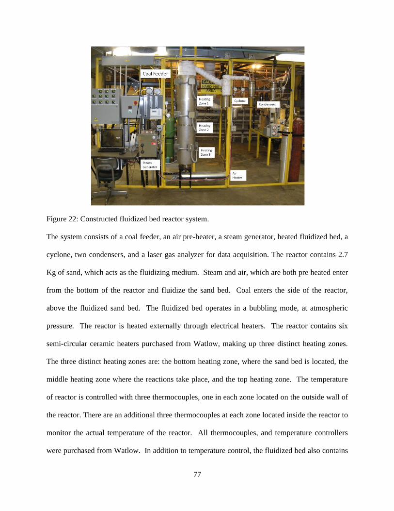
77

Figure 22: Constructed fluidized bed reactor system.

The system consists of a coal feeder, an air pre-heater, a steam generator, heated fluidized bed, a

cyclone, two condensers, and a laser gas analyzer for data acquisition. The reactor contains 2.7

Kg of sand, which acts as the fluidizing medium. Steam and air, which are both pre heated enter

from the bottom of the reactor and fluidize the sand bed. Coal enters the side of the reactor,

above the fluidized sand bed. The fluidized bed operates in a bubbling mode, at atmospheric

pressure. The reactor is heated externally through electrical heaters. The reactor contains six

semi-circular ceramic heaters purchased from Watlow, making up three distinct heating zones.

The three distinct heating zones are: the bottom heating zone, where the sand bed is located, the

middle heating zone where the reactions take place, and the top heating zone. The temperature

of reactor is controlled with three thermocouples, one in each zone located on the outside wall of

the reactor. There are an additional three thermocouples at each zone located inside the reactor to

monitor the actual temperature of the reactor. All thermocouples, and temperature controllers

were purchased from Watlow. In addition to temperature control, the fluidized bed also contains

78

a differential pressure gauge to monitor the pressure inside the bed, and was purchased from

McMaster-Carr. The differential pressure gauge allows insight to what is happening inside the

bed, as far as how the fluidization is occurring and whether or not there are is any plugging or

agglomerations forming. Once the gasification reactions take place, the syngas travels up out of

the reactor, and through a cyclone. The cyclone removes any solid particulate matter, such as ash

or soot and is kept insulated to keep the gas hot. Next, the syngas passes through two condensers

where any remaining organic material, such as tar or aqueous material is removed. Once the

syngas is clean and cooled a sample of it is analyzed in a Laser Gas Analyzer, which measures

the composition of the syngas. The gas analyzer is able to detect hydrogen, oxygen, carbon

monoxide, carbon dioxide, hydrogen sulfide, methane and water vapor. The rest of the syngas

gets pulled out via an inductor system and exits out into the atmosphere. Once all the parts were

in construction took about four months to complete.

4.3 Construction

4.3.1 Unit Operations

4.3.1.1 Air Preheater

The air pre-heater is a heat exchanger that pre-heats the air before entering the reactor chamber.

Pre-heating the air before it enters the reactor is more beneficial to the process, as sending in cold

air would be counterproductive because it will drive the overall temperature of the reactor down

and decrease reaction rate. The challenge was to get an air heater that would be able to heat the

air up as close to the operating temperature as possible. A heat exchanger from Entherm was

selected for the air pre-heater. In the design chapter a target temperature of 400 °C was set for

the temperature of the incoming air into the reactor. In reality, the Entherm heater was capable of

79

producing 500 °C of air at the low flow rate it was operating at. However, due to some heat loss

the actual temperature entering into the reactor was 250 °C.

4.3.1.2 Steam Generator

The steam generator is a device which takes water and heats it up to make steam. This is a single

step device and was implemented for its simplicity. The steam generator was acquired from a

manufacturing company called Reimers Electra Steam. The capacity of the unit is up to 6.4

kg/hr. The unit is connected to the house water line. The manufacturer sets the pressure inside

the unit to 2.4 atm, which is below the pressure in the water line so that it can move into and

through the steam generator. Once the unit builds up steam, the steam is regulated via a medium

flow metering valve, provided by Swagelok. From the valve to the inlet of the reactor, the steam

is super heated by heat tracing the line up to 300 °C.

4.3.1.3 Coal Feeder

The coal feeder consists of a volumetric, single sold screw feeder, with an extension hopper for

additional coal storage. The extension hopper has a capacity holding an additional 4.5 kilograms

of coal. The feeder was provided by the manufacturer Colortronic, and was design to handle a

particle size of 400 microns. The physical properties of the lignite, such as density, as well as

the operating parameters, such as desired coal throughput of 0.4 to 2.3 kg/hr, operating

temperature and pressure were specified. The screw auger of the coal feeder fits into the feeding

port located on the side of the reactor about 46cm above the perforated plate. The screw auger

has a water jacket around it up to the point where it is connected to the feeding port. This was

added as a safety precaution, to prevent heat from the reactor from traveling up and igniting the

coal in the feeder. The water jacket and feeding port were secured together using a tri-clamp

80

sanitary fitting. The screw auger was calibrated using the lignite used for the experiments. The

calibration curve can be seen in appendix D.

4.3.1.4 Fluidized Bed Reactor

The fluidized Bed reactor was constructed from a 3 inch diameter, 5ft high 304 stainless steel

pipe. 304 stainless steel was chosen because it is inexpensive and would suit the application.

The melting point of the steel is 1450 °C, which is significantly higher than the design and

operating temperature of the reactor. The 304 stainless steel has good resistance to oxidation for

intermittent use, up to 870 °C and up to 925 °C It is important to keep the operating temperature

below this upper temperature limit to keep the integrity of the steel intact. The importance of

this upper temperature limit is also there to prevent the formation of ash from occurring, which

can cause fluidization and operational problems. The reactor is externally heated with three

different sets of ceramic heaters, capable of reaching the target operating temperature for

fluidized bed combustion and gasification. These three sets of heaters divide the reactor into

three distinct heating zones, which will be discussed further in the controls section. The reactor

contains 2.7 kg of sand which acts as the fluidizing medium for all the experiments. This

corresponds to a bed height 30.5 cm of sand. All of the experiments were carried out at this bed

height. This amount of sand was based off of preliminary calculations using the coal feeding

port as an initial reference point. . For the distributor plate, a 304 stainless steel perforated plate,

with staggered holes was used. The distributor plate design presented in the design chapter

proved not to be economical when manufacturing it. The metal plate that was used was both

economical and easy to obtain from McMaster-Carr.

4.3.1.5 Cyclone

81

The cyclone is designed to remove any particulate matter, such as ash, and unburned carbon

from the syngas. In the process it is important to place the cyclone right after the fluidized bed,

and to keep the syngas stream as hot as possible. If the cyclone is placed after the gas has been

cooled it could result in damaging effects on the equipment. This is because not only does the

syngas have particulate matter present in it, but it also potentially has tar and water, and if this

mixture is allowed to cool, it could solidify to the cyclone and cause blockages of the syngas as

well as irreparable damage to the cyclone. The cyclone was procured by the company

Colortronic, the same company that provided the coal feeder. The cyclone was originally based

off of the operating design parameters in the previous chapter. In actuality, the operating velocity

of the air was lower than expected, which caused the cyclone not to be as efficient as intended.

In spite of this, the cyclone was still able to knock out some particulate matter. An ash collection

can was attached to the bottom of the cyclone, which allowed any particulate matter that was

being removed from the syngas stream to be collected.

4.3.1.6 Heat Exchangers

The heat exchangers used to condense the organic tar, and aqueous material were built based off

of the design present in the previous chapter. They were built in house, out of stainless steel.

Each of the condensers are the same dimensions with baffles inside to promote turbulence and

increase the residence time in the syngas is in the condenser. There are two condensers to ensure

that all the liquid matter gets removed from the syngas. The target temperature for the first

condenser was 250 °C and was intended to remove most of the tars in this stage. The second

condenser was to remove any remaining tars, light hydrocarbons or water present. The second

condenser had a valve installed at the bottom, so that when the liquid would accumulate during

operation it could be easily drained during operation.

82

4.3.2 Controls

In order to ensure smooth and safe operation the system must be monitored and controlled. For

the fluidized bed system there are two main parameters that are monitored and controlled

including temperature and pressure. The system is equipped with twelve type k thermocouples.

Of these twelve thermocouples half of them control certain parts of the process and the other half

act towards monitoring the temperatures at different parts of the system. There are three heat

tapes present to maintain a minimum temperature for that part of the process. There is one heat

tape for the steam line entering the reactor that is to maintain that the steam entering the reactor

is superheated. The second heat tape is exiting the reactor and entering the cyclone, this is to

keep the syngas from losing all of its heat too fast. The third heat tape is from the cyclone to the

beginning of the first condenser. This is to control the condensation of any organic, tar like

material in the syngas and have it be removed in that condenser. In order to monitor and control

the temperature in the bed three thermocouples are placed axially along the outside of the outside

of the bed. These thermocouples measure the wall temperature in the three different heating

zones in the reactor, these thermocouples also are controlled by temperature controls and are

used to maintain a desired temperature in that zone of the reactor. Similarly, there are three

thermocouples positioned inside the reactor at the same points along the axis as the

thermocouples outside the reactor. These thermocouples display the temperature inside the

reactor and are read only thermocouples. Along with those read only thermocouples inside the

reactor, there is a read only thermocouple exiting the air pre-heater, and one right above the

distributor plate. These two thermocouples act to monitor the actual temperature of the air

entering the reactor, to make sure there is not a drop in temperature before it enters the reactor.

Finally, there is one thermocouple at the inlet to the last condenser to ensure that the syngas is

83

cooled to below the dew point of water. This is necessary for the gas analyzer to measure the

constituents of the syngas. The second parameter of interest is pressure. A low differential

pressure gauge was installed to monitor the change in pressure across the fluidized sand bed.

Monitoring the pressure across the bed gives insight to what is occurring inside the bed. It allows

the operator to identify what kind of fluid flow is present. It also gives insight to any problems

that might be occurring. Agglomeration formation is a common problem in fluidized beds. When

these agglomerates form, as they buildup mass, they can influence the fluidization by causing

channeling or blocking, this phenomena can interpreted through changes in the differential

pressure, and can let the operator know if operating conditions need to be changed to combat the

problem.

4.3.3 Operating Issues

During the commissioning of the system there were some operational challenges needed to be

addressed and worked out. The problems encountered were a result of getting acquainted with

the system. There were two main problems that were encountered, one with the coal feeder,

where the feeder was not able to feed into the reactor due to thermal expansion of the bed; and

with the thermocouples, failing due to the harsh environment and constant cycling of the system.

4.3.3.1 Thermal Expansion of the Bed

Initially, after the heaters around the reactor were installed the reactor would be brought up to the

design temperature of 815 °C. The purpose of this was to perform shakedown testing protocol

for heating the reactor up to operating temperature. Another reason this was done was to “break

in” the reactor and condition the reactor for the prior to performing experiments. When bringing

the reactor up to the necessary temperature, it was observed that thermal stress would create a

problem when trying to deliver coal into the reactor. The reactor is supported by a metal base

84

plate, and is surrounded on all sides with ceramic heaters. The heaters and base plate constrict

the reactor in radial, and downward direction. Therefore, when the reactor was heated, the

thermal stress would force the reactor to expand vertically. Since the coal feeder was mounted in

fixed position, this thermal expansion would shift the coal feeding port on the reactor above the

screw feeder. The result of which was coal was not able to be delivered into the reactor. To

remedy this problem, the coal feeder was housed on a platform which would be able to move in

all directions. This unit consisted of a jack and a trolley and an engine sling. The jack would

allow for the feeder to move in the vertical direction while the trolley allowed it to move in the

horizontal direction. Meanwhile the engine sling would allow the feeder to pivot, see Figure 23.

Figure 23: Coal Feeding system.

This allows the feeder to be inserted in the reactor, and adjust with the thermal expansion every

time the reactor was in operation. Another issue with the coal feeder was clogging, certain

experiments were performed with Kaolinite as an additive which was feed in with the coal

85

through the coal feeder. Kaolinite, is a soft clay mineral, and as such would mix with the coal

and cause clogs in the feeding system. To prevent this clogging, the experiments were done

without the addition to Kaolinite to the bed. Equally important, another operating issue that

came about was the loading and unloading of the sand in and out of the bed. During the

combustion and gasification experiments, samples of the sand bed would need to be taken for

analysis, or sometimes the sand would have to be replenished all together. In the beginning, all

the insulation would have to come off the reactor, and the reactor would have to be dismantled

for the sand to be added, which became quite cumbersome. To solve this issue, a pneumatic

delivery system was employed to deliver the sand through the coal feeding system port, to

replenish the bed with sand, without having to dismantle the entire reactor (Figure 24).

Figure 24: Pneumatic sand replenishing system.

The measured amount of sand would be placed in the bin. The induction system for the reactor is

turned on so that the system has negative pressure. Then, compressed air nozzle is attached to the

86

yellow tubing. Once the valve is open and compressed air is going through the tube a negative

pressure allows the sand to enter the reactor, and results in a replenished fluidized bed. Next,

when experiments were performed in the beginning, a mixture of different operating conditions

was used to get an idea of how the system worked. When ash was collected for these

experiments, the ash reflected those different conditions, and represented every condition that

was performed that day. In order to get a more detailed analysis of the ash, a bypass system was

installed so that the reactor could run continuously and ash samples could be collected in a safe

manner. This allows for better method of sampling while still allowing the system to operate

without shutdown. The last operating issue that had to be dealt with was to make sure the flue

gas was safe to vent off into the atmosphere. This problem was solved by installing a wider pipe

downstream of the system, but before the inductor, that is open to atmosphere. When the

inductor draws the syngas out, since that wider pipe is open to the atmosphere it will draw in

more air which will dilute the syngas stream, allowing it to be vented to the atmosphere in a safe

manner. These operating issues were all encountered while performing shakedown experiments

and characterizing the system as a whole (For the standard operating procedures please see

Appendix A). Once the gasification system was built, and the operating issues were solved,

shakedown commissioning of the system took place. Broadly speaking there were two different

sets of experiments that took place. First, the shakedown experiments were performed. The point

of these experiments were to get the system running, to learn how the system operates, what its

limitations are and what its capabilities are. These experiments include fluidization experiments,

air and oxygen combustion hydro-gasification experiments, as well as calibrating the coal feeder

and steam generator (These calibration curves can be found in Appendix D). After these

experiments were performed, more in depth experiments were carried out, which include air and

87

oxygen gasification. In these experiments, each experiment was timed, the operating conditions

were recorded, and a sample was taken.

4.3.3.2 Thermocouple Problem

When experiments were first conducted, the thermocouples in the reactor kept

failing, specifically, the thermocouple in the middle heating zone. This is the hottest heating zone

because it is right above the fluidized bed and is where the combustion/gasification reactions

take place. Originally type k, grounded 1/8 inch metal sheath thermocouple was used to monitor

the temperature of the bed. Type k thermocouples have a temperature range of −200 °C to

+1250 °C, but there are some conditions that cause acceleration in age and failure of the

thermocouple. Prolonged exposure from 427 to 649 ºC makes the thermocouples age faster.

Type K thermocouples should not be used in reducing environments above 800 °C. This is

because type k thermocouples contain a metal alloy known as Chromel (90% nickel and 10%

chromium). In reducing environments at elevated temperatures, the chromel alloy oxidizes and

corrodes. Due to this alloy degradation, type k thermocouples should not be used in cyclic

oxidizing environments. Changes in temperature result in slight variations in size over long

periods of time, these constant cycles of expansion and contraction can cause metal fatigue

which results in a weaker thermocouple and can ultimately result in failure. Metal fatigue can

occur where the thermocouples are subject to repeated heat stress or extreme temperatures.

Sulfur, which is present in the coal and is released upon combustion and gasification, can react

with the nickel in a type k thermocouple at high temperatures to form nickel sulfide, which

contaminates the thermocouple and causes it to fail. It is also important to note that generally an

ungrounded junction in a thermocouple is more durable than a grounded one. The disadvantage

to an ungrounded junction is that it has a slower response time to temperature changes. While

88

performing experiments, the thermocouples were being subjected to all of the scenarios in which

could cause premature failure; from cycling through oxidizing conditions, to reducing conditions

at high temperature, and to exposure to sulfur. In order to prevent the thermocouples from

failing, and to try to extend the life of the thermocouples for longer periods of time, tougher

thermocouples had to be used. In order to keep costs down, an exotic thermocouple, like

Molybdenum which would be able to handle the high temperatures and changes in environment

could not be implemented. In order to solve the problem, type K thermocouple were still used

but the sheath thickness was increased from 1/8 of an inch to ¼ of an inch, as well an

ungrounded thermocouple was used instead of a grounded one. These measures give the

thermocouple more protection against the harsh environment and extend the life of the

thermocouple. One disadvantage to note from an ungrounded thermocouple compared to a

grounded one is that the ungrounded thermocouple has a slower response time to temperature

changes; this however is not a major issue for the process.

4.4 Ash Sampling System

For experimentation, the fluidized bed system was equipped with places to take samples while

performing experiments. Ash samples are collected from the cyclone via an ash bin. To take a

sample of the ash while the system was running, under a specific set of conditions, a bypass

system was implemented, see figure 25.

89

Figure 25: Bypass system for ash and char sample collection from the cyclone.

This bypass valve was initiated at the end of an experiment to collect and characterize a sample

of the ash for that particular experiment. This bypass allows for a safe way to take a sample by

diverting the syngas away from the cyclone while taking the sample. Equally important, it

allows for the reactor to run continuously in between experiments. A sampling port was also

installed right before the cyclone for isokinetic flyash sampling or bulk filter sampling. The

purpose of these sampling methods is to get an idea of the particle distribution of the particulate

matter present in the gas stream. Preliminary experiments were performed to see whether it

would be particle to perform bulk filter/ isokinetic flyash sampling. The results of those

preliminary tests showed that it is possible to perform those tests, however at the time not very

practical. There were some issues with the syngas being too hot and melting the Teflon tubes

used in the sampling processes. In order to make the sampling more practical, some more

thought would have to go into cooling the syngas more or using metal tubing to connect to the

sampling port. With this problem notwithstanding, it was possible to generate some bulk filters

90

with some ash deposits on them. If of interest to pursue this testing further, a good starting point

for sampling would be to sample for 20 to 25 minutes with a sweep gas of 3 L/min.

4.5 Commissioning of the System

Once the system was constructed, and some of the operating issues were worked out, the

system was commissioned by performing different sets of experiments. First, fluidization

experiments were performed, this was to get an idea of the actual fluidization parameters and

characterize the fluidization characteristics experimentally and compare them to the theoretical

values calculated in the previous chapter. Next a series of shakedown experiments were

performed, where the system was ran under typical operating conditions, with fuel and oxidant

was fed into the reactor to see what kind of syngas composition could be produced. While these

shakedown experiments were performed both tar production and carbon conversion was

investigated. These shakedown experiments establish the operability and capability of the reactor

and set the stage for gasification experiments, both in an air and oxygen atmosphere, which will

be analyzed under specific conditions. These two sets of experiments is the main focus of the

work and as such, the data from those two experiments will be discussed in the results and

discussion chapter.

4.5.1 Fluidization Experiments

First, fluidization experiments were performed, to verify the theoretical fluidization

behavior. The minimum fluidization velocity was found by measuring the pressure drop verses

inlet gas velocity at both ambient figure 26, as well as, operating conditions figure 27.

91

Figure 26: Fluidization experiment, pressure drop Vs velocity at ambient conditions.

In the first fluidization experiment, under ambient conditions a range of flowrates were chosen

based on the rhotometers capabilities. A selected flowrate was chosen and the corresponding

pressure reading was recorded using a differential pressure gauge, with readings in inches of

water. The data was then plotted, in Figure 6 to find the experimental minimum fluidization

velocity of 0.2 m/s. The experiment was then repeated under the planned operating conditions,

of 815 °C (Figure 7).

0

5

10

15

20

25

0 0.05 0.1 0.15 0.2 0.25 0.3 0.35 0.4

ΔP

(in

che

s o

f W

ate

r)

Velocity (m/s)

Fluidization at Ambient Conditions

92

Figure 27: Fluidization experiment, pressure drop Vs velocity at operating conditions.

These experimental results were then compared to how the fluidized bed should behave under

theoretical calculations Figure 28.

Figure 28: Theoretical velocity versus pressure drop across the bed.

In order to generate a velocity vs. pressure drop diagram, different operating velocities, were

used using the Ergun equation. The Ergun equation was used until the minimum fluidization

0

5

10

15

20

25

30

35

40

0 0.05 0.1 0.15 0.2

ΔP

(in

che

s o

f w

ate

r)

V (m/s)

Fluidization at Operating Conditions

0 0.05 0.1 0.15 0.2 0.25 0.3 0.35 0.4

0

10

20

30

40

50

60

70

V (m/s)

ΔP

(in

che

s o

f w

ate

r)

Theoretical

93

velocity was reached, then an empirical correlation provided by (Babu et el) was used once the

bed was fluidized. This was done because the Ergun equation represents a packed bed, while

once the bed becomes fluidized, the pressure stays constant and is better represented by the

empirical correlation. It can be seen that both the theoretical and experimental graphs for

velocity vs. pressure drop at ambient conditions match up fairly well. Based on Figures 27

experimental, operating the minimum fluidization velocity decreased significantly, and could be

recorded as low as 0.03 m/s. this minimum fluidization velocity might even be lower than that,

however it was out of the range of the rhotometers range. This decrease in minimum fluidization

velocity as the temperature increases is expected from the theoretical calculations of the

minimum fluidization velocity. The experimental minimum fluidization velocity was then

compared to the calculated values for both ambient and operating conditions and can be seen in

Table 9.

Table 9: Comparison of theoretical and experimental fluidization values at ambient and

operating conditions. Velocity (m/s) Atmosphere Theoretical Experimental

Minimum Fluidization Ambient 0.24 0.21

Minimum Fluidization Operating 0.1 0.03

Minimum Slugging Ambient 0.29 0.31

Minimum Slugging Operating 0.17 0.07

Equally important, the minimum slugging velocity was also found experimentally for both

ambient and operating conditions in Figures 26 and 27 and compared to its calculated theoretical

value in Table 1. The criteria for determining the slugging phenomena was when the differential

pressure began to develop a fluctuating rhythm, defined by three different pressure reading

associated with one velocity. It can be seen that the experimental values for both the minimum

94

fluidization velocity, as well as the minimum slugging velocity closely match the theoretical

calculated values. As a result of these fluidization experiments, the fluid flow characteristics of

the bed have been established, and an operating range can be employed, to stay within the limits

of the reactor.

4.5.2 Shakedown Experiments

4.5.2.1 Combustion Experiments

Shakedown experiments were performed to get the system in an operating order in order to

conduct meaningful experiments that generated quality data. The first step in accomplishing

this task was to feed coal and air into the reactor and monitor the composition of the syngas to

see how the system responded to different operating conditions. These experiments were

combustion experiments, a known amount of air and coal were fed into the reactor, and flue the

gas composition was recorded. Adjustments were made to see how the system responded to

different operating conditions. Once combustion was running at steady state conditions, a

specific type of condition would be run for that day, whether it be air combustion, air

gasification, hydro-gasification, oxy-combustion or oxy-gasification. In order to transition from

combustion to air gasification, the steam would be injected into the reactor. If the combustion

condition was running at thirty five standard cubic feet per hour, then the air would be cut back

and the steam would make up for the amount of air being cut back by still maintaining an overall

flowrate of thirty five standard cubic feet per hour. The air would be cut back and made up for

with steam until the desired condition for the experiment was reached. It is important to note,

that the reactor always started and ended with air combustion. This way of transitioning between

experiments provided the most straight forward and easy way to transition between combustion

to gasification conditions as well as maintained a constant fluidized bed in the process. This

95

method became the standard for carrying out all of the experiments. Combustion experiments

were performed, followed by oxy-combustion and hydro-gasification. For the combustion

experiments, the coal feed rate was varied from 0.3 to 0.45 lbs/hr and the gas concentration was

investigated at constant air flowrates, as shown in Figure 29.

Figure 29: Combustion shakedown experiment: flue-gas composition at different coal feedrates

This shakedown experiment shows how the gas composition of the flue gas varies with different

coal feed rates. This experiment also shows that combustion is occurring; due to the amount of

carbon dioxide produced. These trends are to be expected, when the amount of coal is increased,

it reacts with the oxygen and produces carbon dioxide. The graph shows that as the coal is

reacting with the oxygen the oxygen is decreasing, and producing carbon dioxide. The graph

also shows that different air flowrates produce different amounts of carbon dioxide. At 45 scfh of

air, the amount of carbon dioxide decreased, implying that at that coal federate 45scfh of air is

falling out of the flammability limits of the coal. Finally this experiment shows the sensitivity

and reliability of the system.

0

5

10

15

20

0.3 0.35 0.4 0.45 Co

nce

ntr

atio

n (v

ol %

)

Feed Rate (lb/hr)

Gas Concentration Vs Feed Rate

O2 at 35 SCFH

CO2 at 35 scfh

O2 at 40 SCFH

CO2 at 40 SCFH

O2 at 45 SCFH

CO2 at 45 SCFH

96

4.5.2.1.1 Oxygen Combustion

In the second shakedown experiment, air was switched to oxygen and an oxy-combustion

experiment was run, to see how much carbon dioxide could be produced in comparison to air

combustion, Figure 30.

Figure 30: Oxygen combustion experiment.

In this experiment the amount of oxygen was varied at a constant flowrate of 0.4 lbs/hr, to see

how much carbon dioxide could be produced. For this system 60% of carbon dioxide was

produced at 10scfh of oxygen. When the amount of oxygen was increased the flammability

limits of the coal was exceeded, which resulted in the system becoming saturated with oxygen.

This inhibited combustion and resulted in a decrease in carbon dioxide production. This

experiment was performed to initiate a starting point for any future research that would be

carried out with oxygen combustion for the system.

4.5.2.1.2 Carbon Conversion

As air combustion experiments were performed, a sample was collected and analyzed for carbon

conversion, figure 31.

0

20

40

60

80

0 10 20 30 40

Gas

Co

nce

ntr

atio

n (

Vo

l%)

Oxygen Flowrate (SCFH)

Oxy Fired Constant Coal Feed Rate

%CO2 (average)

%O2 (average)

97

Figure 31: Air combustion Carbon Conversion at a constant different air flow rates..

The air flowrate was varied over a range of 30 to 45 standard cubic feet per hour. The coal feed

rate was held at a constant rate of 0.4 lbs/hr (120rpm). At that coal feed rate, the optimum

carbon conversion was at a flowrate of 40 SCFH. The carbon conversion ranged from 70 to

86%.

4.5.2.1.3 Hydro-gasification

A hydro-gasification experiment was performed, where only steam was allowed to react with the

coal without the presence of oxygen, to investigate the maximum hydrogen yield, Figure 32.

0

10

20

30

40

50

60

70

80

90

25 30 35 40 45 50

Car

bo

n C

on

vers

ion

(%

)

Air Flowrate (SCFH)

Air Combustion Carbon Conversion

98

Figure 32: Hydro-gasification shakedown experiment.

In this gasification experiment, only steam was used to gasify the coal. The steam as held

constant at 45 SCFH and the coal feed rate was also held constant at 250 rpm. The experiment

was held for twenty five minutes, and the amount of hydrogen was graphed. Figure 9 shows that

under hydro-gasification conditions up to 58% hydrogen can be produced. This experiment can

be compared to an annular externally heated retort. This retort system was a fixed bed gasifier

and operated from 1941 to 1951 on the UND campus (S. A. Benson & Sondreal, n.d.). The retort

produced a syngas with up to 60 % hydrogen. The rest of the syngas components can be

compared in the table 10:

Table 10: Syngas comparison between hydro-gasifcation and literature values. CO % H2 % CH4 %

UND Fluidized Bed 4 54 3

Fixed Bed Retort 13 55 3

Fixed Bed Retort 27 60 5

Table 10 compares syngas composition with the experiments performed in this work with past

hydro-gasification data. For hydrogen production, the syngas composition is comparable to past

0

0.5

1

1.5

2

2.5

3

3.5

4

0

10

20

30

40

50

60

70

0 5 10 15 20 25 30

Gas

Co

mp

osi

tio

n (

Vo

l%)

Time (min)

Hydro-gasification Gasification

H2

CO2

N2

CO

CH4

99

data. The main difference is that there are two different gasification technologies, the hydrogen

retort which uses fixed bed technology, and the fluidized bed technology designed at UND.

4.5.3 Tar Formation

While performing both the shakedown testing, as well as the experiments under gasification

conditions, Tar formation was expected to form. After a day’s worth of experiments, the

cyclone, and two condensers would be cleaned and a sample would be saved for analysis. Tar

was expected to collect in the condensers. Although tar was not formed during each experiment,

there is evidence to suggest, that there was indeed tar formed during some of the hydro-

gasification gasification experiments. To characterize the tar, first a sample of lignite coal was

analyzed using a TA-TGA. A Loss on Ignition test was performed following the ASTM D 7348-

08 standard (Analyses et al., 2009), and can be seen in Figure 33.

100

Figure 33: Loss on Ignition analysis of lignite coal.

The analysis on the coal serves two purposes. First of all, it gives the operator an idea of the

properties of the lignite, how much moisture is present in the coal, as well as how much carbon

the coal contains. Analyzing the coal also acts as a standard to compare potential tar samples to.

In the lignite sample, the large weight loss at 400 °C, along with the exothermic reaction, which

is indicated by the DSC heat curve implies all of the carbon in the coal is being oxidized. If the

samples weight loss curves diverge from this, it could mean that there are other organics formed

which are being burned which could imply tar formation. Next, both liquid and solid samples

were collected from the first and second condensers, respectively and analyzed in TGA. Liquid

samples were collected in the second condenser after each condition, Figure 34.

101

Figure 34: Liquid samples collected at different gasification conditions.

As can be seen from figure 34 the liquid samples changed as the operating conditions changed.

On the right is a vile of water. Each sample becomes darker as the amount of steam increased

and as air is switched to oxygen. From left to right the conditions are as follows: the first sample

is hydro-gasification, the next two are oxygen gasification the next three are air gasification

samples and the last is a vile of water for perspective. Some of these liquid samples were

analyzed in the TGA to see whether they contained any Tars, Figure 35.

102

Figure 35: TGA/DSC analysis of a liquid sample under gasification conditions.

Based on the analysis, most of the sample is water, which can be seen by the majority of the

weight loss at 100 degrees C. However even though there is no apparent change in the mass

after 100 degrees Celsius, the DSC heat curve shows a slight exothermic curve, which suggests

some organic material present in the sample. Even though there is evidence of organic material

present in the sample, further analysis would have to be performed to get a better idea of what its

chemical composition was. Equally important, a couple of different liquid samples were

analyzed and each of the analysis looked similar with no ability to distinguish between them,

despite their different visual appearance shown in Figure 35. A solid sample was also taken

from the first condenser, and analyzed in the TGA, see Figure 36.

103

Figure 36: TGA analysis on a tar sample collected under gasification conditions.

Comparing the solid sample in Figure 33, to a sample of lignite in Figure 10, there appears to be

some evidence that tars form. In the lignite sample, all the water is driven out, and then there is

one large peak, which can be associated with the carbon in the coal being burnt off. In this peak

there is one smooth transition. In the solid sample shown in Figure 33, however, there is not one

large, smooth peak. There are a couple of inflection points, accompanied by a smaller peak. This

shows evidence of other organic material forming with different melting points which can be

associated with these different inflection points, which can be indicative of tar formation.

4.5.4 Bed Agglomeration Formation

While performing both the combustion and gasification experiments, agglomerates were formed,

Figure 14. At first shakedown combustion experiments were ran at 750 °C. The original plan was

104

to perform a set of combustion and gasification experiments at three different temperatures 750,

800 and 850 °C. When the reactor temperature was set for 800 °C for combustion experiments

agglomerations started forming. This was evident by the pressure differential across the bed.

Under normal operating conditions, the pressure gauge will exhibit a range and fluctuate within

that range. However, when agglomeration begins to form and set into the reactor, the pressure

differential decreases and ceases to fluctuate. This caused operational issues, as well as some

damage, which required the reactor to be disassembled. Due to this problem, as well as an

interest to be able to perform a variety of other experiments smoothly and in a timely manner, it

was decided to stick to an operating temperature of 750 °C. For the combustion experiments,

operating at 750 °C solved the problem, as no agglomerates were formed. Figure 37 shows some

agglomeration formation from a fluidized air combustion experiment.

Figure 37: Agglomeration formation under combustion conditions.

For the gasification conditions agglomerations were formed at 750 °C, however Kaolinite was

added to the fluidized bed to help negate the formation of agglomerates. Also, by the time

105

gasification experiments were performed, there was a better understanding on how the reactor

operated. Because of this, although agglomerations were formed during those experiments, they

did not cause damage to the reactor or operational problems. Figure 37 shows some of the

agglomerations formed during combustion experiments at 800 °C, along with the agglomerates,

which are in the middle, are the constituents that form the agglomerates, the lignite on top, along

with the sand on the bottom. A more detailed analysis of the agglomerates will be discussed in

the next chapter.

4.5.5 Summary

During the experimental phase of the project, a fluidized bed was designed for combustion and

gasification, based on fluidization/combustion calculations presented in chapter 3. The system

was built and commissioned. Many improvements had to be made along the way to make the

system run smoothly. These improvements include a bypass system, for more real time

sampling, a modified feeding system, to account for thermal expansion of the reactor, as well as

ensuring the functionality of thermocouples. Equally important, expected operational issues,

such as agglomerate and tar formation were monitored and collected for analysis. A series of

shakedown experiments were undertaken to understand the systems capabilities and limitations.

These shakedown experiments started with fluidization experiments; finding the minimum

fluidization velocity and mapping the fluid regime of the reactor experimentally. Next, different

combustion and gasification experiments were performed to help verify the functionality of the

system. Finally, both air and oxy gasification experiments were run at different operating

conditions and optimized for the production of hydrogen.

106

CHAPTER V

Results and Discussion

5.1 Introduction

Once the system was constructed, shakedown experiments were performed to

commission the system using Center Mine North Dakota Lignite. The shake down

testing consisted of two sets of experiments that included air blown gasification and

oxygen blown gasification. Both sets of experiments were performed at a constant bed

temperature of 750 °C. Multiple experiments were performed and each experiment was

conducted using a fixed set of operating conditions and data was collected at each

condition for a minimum of ten minutes. The composition of the syngas was recorded

over the time for each experiment. Meanwhile, at the end of each experiment a sample of

char was taken from the cyclone, representative of the conditions of the experiment was

collected and analyzed. From this data, the carbon conversion and the cold gas efficiency

were calculated, for both the air and oxygen gasification experiments. Finally, any bed

agglomerated generated during the experiments were collected and analyzed.

5.2 Air Gasification

Air gasification experiments were performed by feeding lignite was fed into the reactor

along with air and steam at 750 °C. The amount of air and steam being fed into the reactor was

held constant at 10 and 25 SCFH respectively, while the amount of coal fed into the reactor was

varied. Each experiment was held for a minimum of ten minutes, while the average time for each

experiment was thirteen minutes. The syngas composition was averaged for each experiment and

107

plotted against the changing coal feed rate, which is expressed as an oxygen to carbon

ratio as shown in Figure 38.

Figure 38: Air gasification: Syngas composition Vs. carbon to oxygen ratio.

Figure 38 shows the changes in syngas composition as a function of C/O. Of the 8 gases

measured, hydrogen sulfide was measured and included in appendix F. The syngas components

which are more abundant are graphed on the left axis, while carbon monoxide and methane are

represented by the right vertical axis. It can be seen from Figure 38 that as the amount of carbon

increases the quality of the syngas improves. The data generated from these experiments were

compared to previous work conducted in a transport reactor gasification (TRIG) ((Kellogg,

Brown and Root (KBR), transport reactor) TRIG on lignite coal reported by Benson and

Sondreal 2010. Table 11.

0

1

2

3

4

5

6

7

8

0

10

20

30

40

50

60

0.5 1 1.5 2 2.5 3 Syn

gas

Co

mp

osi

tio

n C

o, C

H4

(Vo

l%)

Syn

gas

Co

mp

osi

tio

n (

Vo

l%)

C/O

Air Blown Gasification

H2O

H2

CO2

N2

CO

CH4

108

Table 11: Syngas composition of air blown gasification comparison to TRIGTRIG. Gas

Constituent

Run

1

Run

2

Run

3

Run

4

Run

5

Run

6

Run

7

Run

8

Run

9

Run

10

Run

11

TRIGT

RIG

CO 2.13 2.62 2.91 3.25 3.67 4.37 5.2 5.69 6.24 6.96 6.37 8.49

H2S 0.5 0.5 0.6 0.6 0.4 0.5 0.4 0.5 0.3 0.4 0.5 0.2

H2 19.25 23.47 25.06 26.15 27.94 30.86 33.36 34.47 37.1 36.31 36.52 18.14

CO2 20.78 21.23 21.39 21.5 21.35 21.72 21.59 21.37 20.18 20.54 20.66 19.11

CH4 1.28 1.4 1.45 1.52 1.64 1.79 1.8 1.87 1.92 2.06 2.16 3.11

N2 47.82 42.6 40.56 39.05 37.1 33.1 29.76 27.69 25.18 23.4 24.68 50.17

Temperature

°C 750 750 750 750 750 750 750 750 750 750 750 795

C/O 2.48 2.14 1.79 1.59 1.45 1.31 1.1 0.89 0.82 0.76 0.69 3.22

109

The experiment done using the TRIGTRIG (S. A. Benson & Sondreal, n.d.) was performed

using, with air, at 795 °C. The results are comparable to the TRIGTRIG, although the

TRIGTRIG data shows more carbon monoxide, with less hydrogen, and slightly less carbon

dioxide. One explanation of this discrepancy is that the water gas shift reaction is more dominant

in these experiments than the ones performed using the TRIGTRIG. The water gas shift reaction

is:

CO(g) + H2O(g) H2(g) + CO2(g) ΔH=-41 KJ

The water gas shift reaction is sensitive to temperature, at lower temperatures, the reaction favors

the products, and at higher temperatures, it favors the reactants. Since the gas composition is

measured after the gas has been cooled, there is sufficient time for the water gas shift reaction to

take place after the syngas leaves the reactor. For this set of data, a confidence interval was

calculated, Table 12. This was done by calculating the standard deviation for each data point and

performing a t-test. A t-test was performed because the standard deviation of the data was used,

which may not represent the true standard deviation (Lawson, 2001). Also, the sample size was

in the appropriate range for the t-test. Based off of the t-test, the data falls between the

confidence interval with 95% confidence.

110

110

Table 12: Confidence intervals for air gasification.

CO H2O H2S H2 CO2 CH4 N2

95% CI [2.0, 2.2] 95% CI [3.1, 3.1] 95% CI [0.5,0.5] 95% CI [18.6, 19.9] 95% CI [20.7, 20.8] 95% CI [1.3, 1.3] 95% CI [47.1, 48.5]

95% CI [2.6, 2.7] 95% CI [3.0, 3.0] 95% CI [0.5, 0.5] 95% CI [23.1, 23.9] 95% CI [21.2, 21.3] 95% CI [1.4, 1.4] 95% CI [42.1, 43.1]

95% CI [2.8, 3.0] 95% CI [3.0, 3.0] 95% CI [0.6, 0.6] 95% CI [24.8, 25.3] 95% CI [21.4, 21.4] 95% CI [1.4, 1.4] 95% CI [40.2, 40.9]

95% CI [3.2, 3.3] 95% CI [3.1, 3.1] 95% CI [0.6, 0.6] 95% CI [25.9, 26.4] 95% CI [21.5, 21.5] 95% CI [1.5, 1.5] 95% CI [38.8, 39.3]

95% CI [3.5, 3.8] 95% CI [3.2, 3.2] 95% CI [0.3, 0.4] 95% CI [27.1, 28.8] 95% CI [21.0, 21.7] 95% CI [1.6, 1.6] 95% CI [35.9, 38.3]

95% CI [4.2, 4.5] 95% CI [3.2, 3.2] 95% CI [0.5, 0.5] 95% CI [30.4, 31.3] 95% CI [21.7, 21.8] 95% CI [1.8, 1.8] 95% CI [32.5, 33.7]

95% CI [5.1, 5.3] 95% CI [3.1, 3.2) 95% CI [0.4, 0.4] 95% CI [33.1, 33.6] 95% CI [21.5, 21.7] 95% CI [1.8, 1.8] 95% CI [29.3, 30.2]

95% CI [5.6, 5.7] 95% CI [3.2, 3.2] 95% CI [0.5, 0.5] 95% CI [34.3, 34.6] 95% CI[21.3, 21.4] 95% CI [1.9, 1.9] 95% CI [27.5, 27.8]

95% CI [6.2, 6.3] 95% CI [3.2, 3.2] 95% CI [0.3, 0.3] 95% CI [36.6, 37.6] 95% CI [19.9, 20.5] 95% CI [1.9, 1.9] 95% CI [24.9, 25.5]

95% CI [6.9,7.0] 95% CI [2.9, 3.1] 95% CI [0.4, 0.5] 95% CI [36.2, 36.4] 95% CI [20.5, 20.6] 95% CI [2.0,2.0] 95% CI [23.2, 23.6]

95% CI [6.3, 6.4] 95% CI [3.2, 3.2] 95% CI [0.4, 0.5] 95% CI [36.0, 37.1] 95% CI [20.3, 21.0] 95% CI [2.2, 2.2] 95% CI [24.4, 24.9]

111

An experiment consisted of generating data for a set time and then changing the coal feed rate.

Data would be recorded once the reactor reached steady state. After each experiment, the bypass

would be initiated, and an ash sample, from the cyclone, would be collected. These ash samples

were analyzed in a muffle furnace in accordance with ASTM standard D 7348-08, Loss on

Ignition of Solid Combustion Residues (Analyses et al., 2009). The data to these tests can be

found in appendix B. This test was done to determine the amount of organic material left in the

sample. All of the organic material was assumed to be carbon. The carbon present in the ash,

along with the carbon generated in the Syngas, was combined to calculate the overall carbon

conversion for each set of experiments, Figure 39.

Figure 39: Air gasification: Carbon conversion at different carbon to oxygen ratios.

From Figure 39, as the oxygen to carbon ratio is increasing the efficiency is increasing. This is to

be expected because the amount of oxygen remains constant, as the coal feed rate is increasing,.

When these results are compared to experiments performed at the TRIG the range for carbon

Trig

0

20

40

60

80

100

0 0.5 1 1.5 2 2.5 3 3.5

Car

bo

n C

on

vers

ion

(%

)

C/O

Air Blown Gasification Carbon Conversion

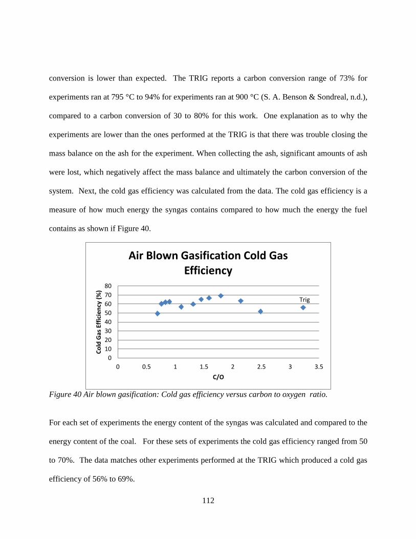
112

conversion is lower than expected. The TRIG reports a carbon conversion range of 73% for

experiments ran at 795 °C to 94% for experiments ran at 900 °C (S. A. Benson & Sondreal, n.d.),

compared to a carbon conversion of 30 to 80% for this work. One explanation as to why the

experiments are lower than the ones performed at the TRIG is that there was trouble closing the

mass balance on the ash for the experiment. When collecting the ash, significant amounts of ash

were lost, which negatively affect the mass balance and ultimately the carbon conversion of the

system. Next, the cold gas efficiency was calculated from the data. The cold gas efficiency is a

measure of how much energy the syngas contains compared to how much the energy the fuel

contains as shown if Figure 40.

Figure 40 Air blown gasification: Cold gas efficiency versus carbon to oxygen ratio.

For each set of experiments the energy content of the syngas was calculated and compared to the

energy content of the coal. For these sets of experiments the cold gas efficiency ranged from 50

to 70%. The data matches other experiments performed at the TRIG which produced a cold gas

efficiency of 56% to 69%.

Trig

0

10

20

30

40

50

60

70

80

0 0.5 1 1.5 2 2.5 3 3.5

Co

ld G

as E

ffic

ien

cy (

%)

C/O

Air Blown Gasification Cold Gas Efficiency

113

5.3 Oxygen Gasification

Along with the air gasification experiments, oxygen blown gasification

experiments were performed in a similar fashion to the air blown experiments. The main

difference between these two sets of experiments is that air is used as the oxidant for the

air blown experiments and pure oxygen is used for the oxygen blown experiments. Three

sets of experiments were performed to in order to optimize the reactor for syngas

production. The first set of oxygen blown experiments was to find the optimum amount

of oxygen, while maintaining a constant amount of coal and steam. The second set of

experiments was to find the optimum amount of coal fed into the reactor, while the third

set of experiments was to find the optimum amount of steam. For the first set of

experiments, the composition of the syngas was plotted vs. an increase in oxygen to

carbon ratio as shown in Figure 41.

Figure 41: Oxygen gasification: Syngas composition versus oxygen to carbon ratio.

0

2

4

6

8

10

12

14

16

18

0

10

20

30

40

50

60

0.75 0.95 1.15 1.35 1.55 1.75 Syn

gas

Co

mp

osi

tio

n C

O, C

H4

(Vo

l%)

Syn

gas

Co

mp

osi

tio

n (

Vo

l%)

O/C

Oxygen Gasification

%H2

% CO2

% H2O

%CO

% CH4

114

From Figure 5-4it can be seen that as the oxygen to carbon ratio is increased the amount of

hydrogen decreased. For each of these experiments, the gas composition data is expressed in

table 13 so that it can be compared to data gathered from the literature.

Table 13: Comparison of UND data with TRIG for oxygen blown gasification. Gas

Constituent Run 1 Run 2 Run 3 TRIG Run 4 Run 5 Run 6

H2 49.2 42.2 38.5 37.8 37.6 33.7 31.6

CO 12.2 13.6 14.5 26 15.8 16.2 13.2

CO2 30.8 31.6 32.7 29.5 36 38.5 34.4

CH4 3.2 2.9 2.5 5.2 2.6 2.3 2.3

H2S 0.4 0.6 0.6 0.5 0.7 0.6 0.5

N2 0.2 2.6 3.3 0.1 1.5 2.4 13.6

Temperature

°C 750 750 750 900 750 750 750

O/C 0.8 0.9 1.1 0.34 1.2 1.4 1.6

Oxygen blown gasification experiments were performed at the TRIG with lignite as the fuel

source, at a temperature of 900 °C. The results of the gas composition with the experiments

performed in this work are comparable to the work done at the TRIG. The gas composition from

the TRIG experiment fell right in between the experiments performed in this work. Similarly to

the air blown experiments, a mass balance was performed on the oxygen blown gasification

experiments as well. At the end of each experiment, an ash sample was collected and analyzed

for its carbon content, that along with the carbon present in the syngas was used for the a mass

balance and a carbon conversion was calculated and shown in figure 42.

115

Figure 42: Gasification: carbon conversion versus oxygen to carbon ratio.

The carbon conversion for the oxygen blown gasification experiments were generally higher than

in the air blown gasification experiments, 40 to 75% for oxygen blown compared to the 30 to

80% of air blown experiments. Furthermore, the carbon conversion for the work performed in

this work is lower than that reported by the TRIG, of 94%. One of the reasons for the lower

carbon conversion is similar to the reason why the air blown gasification carbon conversion was

low. That is there was some trouble closing the mass balance due to some errors in collecting the

ash samples for the experiments. Equally important, the experiments performed at UND were

done at a lower temperature of 750 °C, this lower temperature would contribute to the reason

why the carbon conversion is lower. Next the cold gas efficiency for each oxygen blown

experiment was performed, and compared to data from the TRIG as illustrated in Figure 43.

Trig

0

20

40

60

80

100

0 0.5 1 1.5 2 Ove

rall

Car

bo

n C

on

vwe

rsio

n (

%)

O/C

Oxygen Blown Gasification Carbon Conversion

116

Figure 43: Oxygen gasification: Cold gas efficiency at different oxygen to carbon ratios.

Based on Figure 43 the cold gas efficiency for oxygen blown gasification is between 70 and

90%, which is higher than the air-blown gasification experiments. The cold gas efficiency

reported by the TRIG is 79% (S. A. Benson & Sondreal, n.d.). Based on this value, the data is

comparable to other works. A summary of both the carbon conversion and cold gas efficiency

data can be seen in Table 14

Table 14: Comparison of carbon conversion of both air and oxygen blown experiments with

TRIG.

Trig

0

20

40

60

80

100

0 0.5 1 1.5 2

Axi

s Ti

tle

Axis Title

Oxygen Blown Gasification Cold Gas Efficiency

117

Table 14: Comparison of carbon conversion and cold gas efficiency

Carbon Conversion

UND EERC

Oxygen Blown 40-75% 94%

Temperature °C 750 900

Air Blown 30-80% 96%,73%

Temperature °C 750 940,795

Cold Gas Efficiency

UND EERC

Oxygen Blown 70-91% 79%

Temperature °C 750 900

Air Blown 50-70% 69%, 56%

Temperature °C 750 940,795

Once the optimum amount of oxygen needed for hydrogen generation was found. The amount of

coal was varied to further maximize hydrogen production. Similar to the last set of experiments,

the amount of oxygen was fixed at 5 SCFH and the amount of steam was fixed at 25 SCFH while

the amount of coal was varied. The resulting syngas composition can be seen in the Figure 44.

Figure 44: Oxygen gasification: Syngas composition versus steam to carbon ratio.

0

2

4

6

8

10

12

0

10

20

30

40

50

60

0.8 0.9 1 1.1 1.2 1.3 1.4 Syn

gas

Co

mp

osi

tio

n C

O, C

H4

(Vo

l%)

Syn

gas

Co

mp

osi

tio

n (

Vo

l %)

H2O/C

Oxygen Gasification

H2

CO2

H2O

CO

CH4

118

Three different coal feed rates were selected to determine syngas composition as a function of

steam to carbon ratio. From these sets of experiments it was found that feeding in coal with a

steam to carbon ratio of about 1 is where maximum hydrogen production was reached. When the

amount of coal was increased further with a fixed amount of oxygen and steam, the amount of

hydrogen decreased, implying that at those conditions the hydrogen production reached its peak

value at a steam to carbon ratio that is close to unity. This set of experiments, combined with the

next set of experiments, where the amount of coal and oxygen were held constant at the values

where each produced a maximum amount of hydrogen. The amount of steam was varied to see

how the amount of steam introduced into the reactor would influence the syngas composition.

The results of these experiments can be seen in the Figure 45.

Figure 45: Oxygen gasification: syngas composition versus steam to carbon ratio.

From Figure 45 the amount of steam to carbon ratio that produces the most hydrogen is slightly

greater than unity. As the amount of steam is increased the system becomes saturated with steam

and there is too much steam to react with the carbon available so the hydrogen production

-0.3

0.2

0.7

1.2

1.7

2.2

2.7

3.2

3.7

0

10

20

30

40

50

60

0.5 1 1.5 2 2.5 Syn

gas

Co

mp

osi

tio

n C

O, C

H4

(Vo

l%)

Syn

gas

Co

mp

osi

tio

n (

Vo

l %)

H2O/C

Oxygen Gasification

%H2

%CO

% CO2

% H2O

% CH4

119

decreases. This set of experiments also shows the presence, and influence the water gas shift

reaction has on syngas composition. The water gas shift reaction produces hydrogen and carbon

dioxide at the expense of carbon monoxide, since the system is saturated with hydrogen the

carbon monoxide is consumed and converted to carbon dioxide, which is evident from Figure 45.

5.4 Oxygen gasification summary

Based on the oxygen fired gasification experiments, the system was optimized for

maximum hydrogen production of 54% by performing three sets of experiments on each

operating condition, oxygen content, coal content and steam content. Based on these

three experiments the operating conditions which produced the most amount of hydrogen

were 5 SCFH of oxygen and 1.6 lbs./hr. of coal and 25 SCFH of steam. As the amount of

oxygen or steam increased from these conditions, the amount of hydrogen decreased. It is

important to note the fluidization aspect of these conditions. The overall volumetric flow-

rate of the oxygen and steam combined at optimum hydrogen production is 35 SCFH

which corresponds to an operating velocity of 0.06 m/s. If this operating velocity is

compared to the table summary in chapter four it can be seen that this operating velocity

is just under the experimental value found for the minimum slugging velocity. This

demonstrates how the chemical reactions, and quality of syngas is affected by the

fluidization characteristics of the reactor. This can be seen in both sets of oxygen

gasification experiments. At a fixed amount of oxygen and coal, as the steam is increased

the overall fluidization quality changes from a bubbling to slugging regime, for a

bubbling bed, this can create temperature irregularities decreases mixing in the reactor,

120

which will have a negative impact on the ability to carry out the chemical reactions for

gasification, and ultimately produce a lower quality syngas.

5.5 Agglomerate Generation

During the course of performing these experiments, bed agglomerations from the

reaction of coal impurities with silica sand bed particles form by bonding bed particles.

These agglomerates were generated for both higher O/C typical of combustion and lower

O/C typical of gasification conditions. The agglomerations were more prevalent under

lower O/C testing. After performing experiments the reactor is shut down and cleaned

out. In between cleaning the reactor and preparing it for the next set of experiments these

agglomerations were collected and prepared for characterization using scanning electron

microscopy and x-ray microanalysis techniques (SEM) developed by Microbeam

Technologies Inc. The SEM morphological analysis method provides images and

chemical composition of selected features.

5.5.1 Agglomerate Sample Preparation

Once the agglomerate samples were collected they needed to be prepared for

SEM analysis. The procedure for preparing each samples are as follows:

First the sample is set in an epoxy mold and let the sample set in the epoxy overnight.

Next the sample undergoes a series of polishing grits. Polishing the sample both makes a

single uniform plane from which the microscope can effectively use to gather

information, as well as act to buff out any scratches that are present in the sample. First

the sample gets polished through a series of rough grit sand papers via a turntable. The

sample undergoes polishing from 200 grit, 320 grit, 400 grit, 600 grit, and 800 grit. With

121

each stage lape oil is used to promote smooth, uniform polishing. After, the sample has

been polished with the series of rough sand paper, it gets sonicated in toluene for five

minutes, which acts to clean the newly polished surface. Then the sample goes through

two fine grit polishing. The sample gets polished with a six micron diamond paste and

sonicated in toluene a second time. Finally the sample gets polished down with a one

micron diamond paste and sonicated in toluene. This produces a sample with a smooth

surface and can be seen in the Figure 46:

Figure 46: Polished agglomerate samples before carbon coat.

122

Once the sample has been polished, it gets carbon coated using an Emitech K450 carbon coater.

Carbon coating the sample, prevents the sample from charging inside the microscope.

5.5.2 Combustion Generated Agglomerates

Combustion Generated Morphology

Morphological analysis of combustion generated agglomerates is summarized in Table

15, with corresponding backscattered electron images in Figures 47A and 47B. The large

particles in Figures 47A and 47B are silica particles from the sand bed, these particles are held

together by bonding material (points 1-10 in Figure 47A, and points 4-11 in Figure 47B). The

bonding material for figure 10A contains silica and calcium with minor amounts of other

elements such as iron and sodium. The bonding material in Figure 47B contains silica, barium

and calcium. To a lesser extent the bonding material contains aluminum, iron and sodium..

123

Table 15: Morphology analysis results of Combustion Generated impurities. Elemental results expressed as weight percent,

normalized to 100%. Figure Point Description Na Mg Al Si S Cl K Ca Fe Ba O

47A 1 Bonding Material 4.8 2.7 11.1 32.6 0.0 0.0 0.0 9.0 4.0 0.0 35.8

2 Bonding Material 1.5 1.7 8.9 39.5 0.0 0.0 0.0 14.7 6.6 0.0 27.1









47B 1 Large Particle 0.0 0.0 0.2 78.5 0.2 0.2 0.2 0.3 0.4 0.9 19.1

2 Large Particle 0.0 0.0 0.7 61.7 0.3 0.3 0.2 0.1 0.2 0.6 36.1

3 Large Particle 0.0 0.0 0.2 79.7 0.2 0.1 0.2 0.2 0.4 0.7 18.4














Average 2.0 1.4 6.4 38.2 0.4 0.2 0.2 10.5 7.0 12.9 26.0

124

A. B. Figure 47: Backscattered electron images of combustion generated impurities showing

morphology analysis points.

5.5.3 Gasification Agglomerates

Air gasification agglomerate (1-1B) morphology

Morphological analysis of air gasification (sample 1-1B) generated agglomeration is

summarized in Table 16, with corresponding backscattered electron images in Figures 48A and

48B. The large, darker, particles in figures 48A and 48B are silica particles from the sand bed,

these particles are held together by bonding material (points 1-10 in Figure 48A, and 48B). The

bonding material for both Figures 48A and 48B contain silica and calcium rich phases, there are

also a significant amount of iron rich phases present. Sodium is also present in the bonding

material, though to a lesser extent than the calcium, silica, and iron.

125

Table 16: Morphology analysis results of Air Gasification (1-1B) Generated impurities.

Elemental results expressed as weight percent, normalized to 100%.

Figure

Point

Description

Na

Mg

Al

Si

K

Ca

Ti

Fe

O

48A 1 Bonding Material 0 0 0.3 0.2 0 0.2 0 90.6 8.7

2 Bonding Material 8.3 1.7 3.7 22.3 1.4 8.5 0.2 9.2 44.6


4 Bonding Material 0.2 0.2 0.3 50.2 0 0 0.1 0.3 48.7




8 Bonding Material 2.5 4.4 6.1 15.3 0.2 31.0 0 2.9 37.5



48B 1 Particle 0 0.2 0 54.2 0 0.2 0.2 0.2 45.0




5 Bright Particle 7.2 1.7 4.0 18.2 0.7 8.0 0.2 4.3 55.7



8 Bright Particle 5.6 3.6 6.3 10.6 0.3 12.8 0.3 2.1 58.4



Average 5.7 2.3 4.4 19.5 0.5 11.1 0.3 10.23 46.0

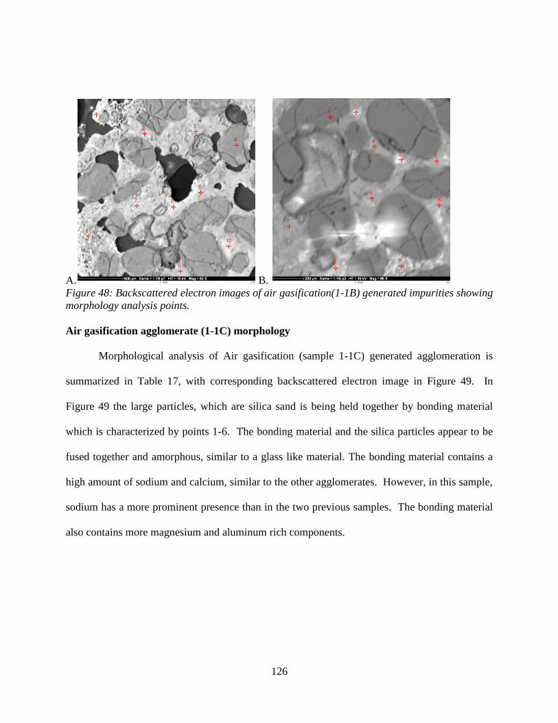
126

A. B.

Figure 48: Backscattered electron images of air gasification(1-1B) generated impurities showing


Air gasification agglomerate (1-1C) morphology

Morphological analysis of Air gasification (sample 1-1C) generated agglomeration is

summarized in Table 17, with corresponding backscattered electron image in Figure 49. In

Figure 49 the large particles, which are silica sand is being held together by bonding material

which is characterized by points 1-6. The bonding material and the silica particles appear to be

fused together and amorphous, similar to a glass like material. The bonding material contains a

high amount of sodium and calcium, similar to the other agglomerates. However, in this sample,

sodium has a more prominent presence than in the two previous samples. The bonding material

also contains more magnesium and aluminum rich components.

127

Table 87: Morphology analysis results of Air Gasification (1-1C) Generated impurities.

Elemental results expressed as weight percent, normalized to 100%. Figure Point Description Na Mg Al Si S K Ca Ti Fe O

49 1 Bonding Material 12.6 4.5 7.1 6.2 0.0 0.4 18.5 0.4 7.7 42.6

2 Bonding Material 12.2 22.9 5.0 2.1 0.2 0.1 7.0 0.2 7.6 42.9





Average 14.1 7.7 7.8 4.8 0.5 0.2 15.2 0.3 5.7 43.7

Figure 49: Backscattered electron images of air gasification(1-1B) generated impurities showing


Air Gasification agglomerate (1-1C) SEMPC The scanning electron microscope point count method provides quantitative chemical

composition data for fly ash and deposits. The point count method uses this chemical

composition method to classify each point it encounters. From this method, it is possible to

directly determine the reactions and interactions that occurred during the deposit formation

(Meuzelaar, 1992). Typically a grid with one hundred points, with predetermined dimensions is

used to analyze the sample. The microscope then analyzes each point for chemical composition

128

and classifies that point into minerals that are associated with that chemical composition. Three

grids, totaling 300 individual analysis points across the agglomerate cross section were analyzed.

The elemental composition of each point was acquired and this information entered into a

computer program to determine the phases (crystalline and amorphous/glass/unclassified)

present as well as abundance. The results of this analysis are summarized in Table 18 with

corresponding backscattered electron images in Figure 50. The analysis shows the agglomerate

to be comprised mainly of unclassified glass or amorphous material (97.2%). Out of the minerals

that could be identified, the agglomerate consisted of dicalcium silicate (1.2%) calcium oxide

(0.8%), and gehlenite (0.8%). The unclassified points are those points whose elemental

composition does not fit the mineral criteria for this analysis.

Figure 50: Backscattered electron images of Air gasification (1-1C) generated impurities

showing SEMPC analysis grids.

Table 98: SEMPC analysis results of Air Gasification (1-1C). Results expressed as weight

percent, normalized to 100%. Silicate and other Crystalline Phases

Gehlenite 0.8

Dicalcium Silicate 1.2

Oxide or Carbonate Phases

Calcium Oxide 0.8

Unclassified and designated Amorphous Phases

Unclassified 97.2

129

The average elemental composition of bulk sample and the unclassified points is

summarized in Table 19. The bulk sample is mostly calcium, silicon and oxygen with small

amounts of sodium. The unclassified points are enriched in sodium, magnesium, aluminum,

silicon, and iron.

Table 19: SEMPC elemental results of Air Gasification (1-1C). Elemental results expressed as

weight percent, normalized to 100%. Na Mg Al Si P S Cl K Ca Ti Mn Fe Ba O

Bulk 4.5 2.2 2.2 9.8 0.1 0.5 0.1 0.5 42.4 0.1 0.1 2.9 1.0 33.6

Unclassified 13.0 4.6 8.8 6.6 0.5 0.4 0.1 0.3 19.9 0.2 0.1 5.9 0.6 39.1

The three main constituents out of the point count data for both the bulk and unclassified

elements are displayed in a ternary diagram in figure 51.

Figure 51: Ternary Diagram of SEMPC of sample 1-1C

The ternary diagram shows that the majority of the composition of the bonding material comes

from calcium, sodium, and silicon oxide.

130

Air gasification agglomerate (1-1F) morphology

Morphological analysis of Air gasification (sample 1-1F) generated agglomeration is

summarized in Table 20, with corresponding backscattered electron images in Figure 52. In


which is characterized by points 1-8. In figure 52A there are distinct particles, the silica sand

particles and the bonding material that binds them together. However, in Figure 52 B the

bonding material and the silica particles appear to be fused together and in an amorphous state.

The bonding material contains a high amount of calcium, along with silicon and aluminum and

to a lesser extent, sodium.

131

Table 20: Morphology analysis results of Air Gasification (1-1F) Generated impurities.


52A 1 Bonding

Material

10.8 5.6 21.1 14.3 0.0 0.1 7.2 0.3 9.0 31.6

2 Bonding

Material

6.3 4.3 12.6 11.7 0.4 0.4 34.1 0.5 3.2 26.5

3 Bonding

Material

3.4 5.2 8.9 14.6 0.2 0.7 37.4 0.8 3.6 25.3

4 Bonding

Material

9.5 5.1 11.7 13.3 0.6 2.9 24.5 0.6 10.6 21.1

5 Bonding

Material

10.2 4.6 9.3 12.6 1.0 3.1 25.7 0.6 4.0 29.0

6 Bonding

Material

7.1 3.5 12.9 8.0 0.2 0.7 20.9 0.5 26.9 19.4

7 Bonding

Material

7.1 5.1 10.9 12.3 1.0 1.4 33.3 0.6 4.1 24.2

8 Bonding

Material

9.4 5.9 5.7 14.7 0.3 0.9 32.2 0.2 4.9 25.9

52 B 1 Bonding

Material

16.0 2.9 8.0 11.9 0.3 0.8 30.4 0.2 5.1 24.4

2 Bonding

Material

6.0 0.9 1.7 14.3 0.4 0.8 43.3 0.7 7.9 24.1

3 Bonding

Material

14.5 4.6 10.2 10.7 0.7 0.6 27.2 0.3 6.0 25.2

4 Bonding

Material

8.9 6.1 8.7 8.9 1.5 1.2 23.4 0.3 17.5 23.5

5 Bonding

Material

13.8 5.8 11.1 4.3 0.3 0.6 24.8 0.4 12.1 27.1

6 Bonding

Material

10.8 3.1 13.5 4.5 0.4 0.7 29.7 0.4 11.0 26.0

7 Bonding

Material

11.7 4.4 10.4 9.5 0.4 0.4 29.3 0.5 8.7 24.7

Average 9.7 4.5 10.4 11.0 0.5 1.0 28.2 0.5 9.0 25.2

132

A. B.

Figure 52: Backscattered electron images of air gasification (1-1F) generated impurities

showing morphology analysis points.

Air Gasification (1-1F) SEMPC

Three grids, totaling 300 individual analysis points across the agglomerate cross section

were analyzed. The elemental composition of each point was acquired and this information

entered into a computer program to determine mineral phases present as well as abundance. The

results of this analysis are summarized in Table 21 with corresponding backscattered electron

images in Figure 53. The analysis shows the agglomerate to be comprised mainly of unclassified

material (95.4%). Of the minerals that were identified, the agglomerate consisted of dicalcium

silicate (1.8%) calcium oxide (1.1%), and gehlenite, spurrite, quartz, iron oxide and ankerite at

(0.8%). The unclassified points are those points whose elemental composition does not fit the

mineral criteria for this analysis.

133

Figure 53: Backscattered electron images of Air gasification (1-1F) generated impurities

showing SEMPC analysis grids.

Table 21: SEMPC analysis results of Air Gasification (1-1F). Results expressed as weight


Gehlenite 0.4

Dicalcium Silicate 1.8

Spurrite 0.4


Quartz 0.4

Iron Oxide 0.4

Calcium Oxide 1.1

Ankerite (Ca,Mg,Fe)CO31 0.4


Unclassified 95.4

1 likely an phase


summarized in Table 22. The bulk sample is mostly calcium and iron with smaller amounts of

sodium, aluminum, and silicon. The unclassified points are also enriched in calcium, and oxygen

along with iron, sodium, aluminum, magnesium, and silicon.

Table 22: SEMPC elemental results of Air Gasification (1-1F). Elemental results expressed as

weight percent, normalized to 100%. Na Mg Al Si P S Cl K Ca Ti Mn Fe Ba O

Bulk 8.9 3.8 9.2 8.7 0.4 0.5 0.3 0.5 24.3 0.3 0.1 17.0 1.0 24.9

Unclassified 10.2 3.8 9.0 8.0 0.5 0.3 0.1 0.5 27.5 0.2 0.1 8.1 0.9 30.6

The three most abundant elements were taken from the SEMPC data both bulk and unclassified

normalized and plotted on a ternary diagram, Figure 54

134

Figure 54: Ternary Diagram of SEMPC of sample 1-1F.

Based on Figure 54 the majority of the composition of the bonding material comes from calcium

and oxygen interactions with a small contribution from sodium.

Air gasification agglomerate (11-1B) morphology

Morphological analysis of Air gasification (sample 11-1B) generated agglomeration is


Figure 55 the large particles have fused together with the bonding material. The composition of

the agglomerate consists mainly of calcium, silicon, and aluminum, which is represented in

pictures 55A and 55B points 1-6 and 1-7 respectively. Along with the main constituents, the

agglomerate also contains amounts of sodium, magnesium and iron.

135

Table 23: Morphology analysis results of Air Gasification (11-1B) Generated impurities.


55A 1 Bonding

Material

4.2 4.6 4.1 9.8 0.1 0.2 21.1 0.1 2.5 53.3

2 Bonding

Material

3.4 5.1 4.9 8.7 0.0 0.3 21.5 0.2 3.7 52.4

3 Bonding

Material

8.5 3.1 8.0 5.9 0.1 0.3 12.9 0.4 7.5 53.3

4 Bonding

Material

8.0 3.3 7.6 6.3 0.3 0.3 15.4 0.3 4.0 54.6

5 Bonding

Material

3.5 5.0 3.6 9.5 0.0 0.1 23.5 0.4 2.8 51.6

6 Bonding

Material

4.1 3.0 10.1 7.4 0.6 0.7 18.1 0.6 9.7 45.7

55B 1 Bonding

Material

2.8 5.4 3.6 10.3 0.6 0.5 26.6 0.3 5.5 44.5

2 Bonding

Material

6.8 5.1 8.6 9.7 0.5 0.1 23.5 0.6 6.3 38.7

3 Bonding

Material

8.7 4.6 10.0 12.5 0.4 0.9 21.2 0.8 5.5 35.5

4 Bonding

Material

1.6 3.3 12.9 5.9 0.0 0.0 20.6 0.3 4.3 51.1

5 Bonding

Material

6.1 4.2 9.8 9.4 0.3 0.1 22.8 0.9 11.0 35.6

6 Bonding

Material

3.1 4.3 8.9 9.6 0.8 0.3 21.6 0.8 12.1 38.5

7 Bonding

Material

2.0 6.0 1.3 13.6 0.1 0.7 33.0 0.3 1.3 41.8

Average 4.8 4.4 7.2 9.1 0.3 0.3 21.7 0.5 5.9 45.9

A. B.

Figure 55: Backscattered electron images of air gasification (11-1B) generated impurities


136

Oxygen gasification agglomerate (12-1) morphology

Morphological analysis of air gasification (sample 12-1) generated agglomeration is


Figure 5-20 the large particles, which are silica sand is being held together by bonding material

which is characterized by points 1-12 in Figure 56A and points 1-9 in Figure 56B. In both

figures the bonding material has fused together with the large particles. The agglomeration

consists of calcium, silicon, aluminum and iron rich phases.

Table 24: Morphology analysis results of Oxygen Gasification (12-1) Generated impurities.

Elemental results expressed as weight percent, normalized to 100%. Figure Point Description Na Mg Al Si K Ca Ti Fe O

56A 1 Bonding Material 6.3 2.3 11.5 22.6 0.9 18.4 0.6 7.3 30.1


3 Dark Particle 0.2 0 0 56.0 0 0 0 0.3 43.4










56B 1 Bonding Material 2.3 2.1 9.3 16.6 0.9 15.8 0.7 16.4 35.8


3 Dark Particle 2.3 0.9 33.3 22.4 0.4 0.1 0.2 0.6 39.8







Average 3.8 2.7 11.7 23.4 0.8 14.8 0.6 10.3 32.0

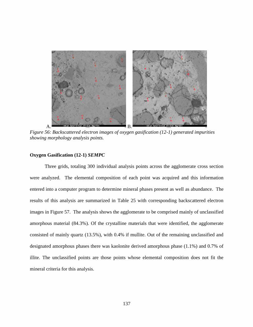
137

A. B.

Figure 56: Backscattered electron images of oxygen gasification (12-1) generated impurities


Oxygen Gasification (12-1) SEMPC






amorphous material (84.3%). Of the crystalline materials that were identified, the agglomerate

consisted of mainly quartz (13.5%), with 0.4% if mullite. Out of the remaining unclassified and

designated amorphous phases there was kaolonite derived amorphous phase (1.1%) and 0.7% of

illite. The unclassified points are those points whose elemental composition does not fit the

mineral criteria for this analysis.

138

Figure 57: Backscattered electron images of Oxygen gasification (12-1) generated impurities

showing SEMPC analysis grids

Table 25: SEMPC analysis results of Oxygen Gasification (12-1). Results expressed as weight


Mullite 0.4


Quartz 13.5


Unclassified 84.3

Kaolinite Derived 1.1

Illite 0.7


summarized in Table 26. The bulk sample is mostly Silicon and oxygen with smaller amounts of

sodium, and aluminum. The unclassified points are also enriched in predominantly Silica,

oxygen aluminum, calcium, and iron. Based on the SEMPC analysis along with the

corresponding figure 57, this sample formed amorphous glass phase agglomerate.

Table 26: SEMPC elemental results of Oxygen Gasification (12-1). Elemental results expressed

as weight percent, normalized to 100%. Na Mg Al Si P S Cl K Ca Ti Mn Fe Ba O

Bulk 1.1 0.1 4.3 50.3 0.5 0.2 0.5 0.2 0.5 0.2 0.1 0.5 0.2 41.4

Unclassified 3.3 1.4 21.5 19.7 2.6 0.1 0.2 0.8 7.2 1.0 0.1 7.2 0.6 34.4

139


normalized and plotted on a ternary diagram, Figure 58

Figure 58: Ternary Diagram of SEMPC of sample 12-1

Based on Figure 58 the majority of the composition of the bonding material comes from oxygen,

and silicon, interactions with a small contribution from aluminum.

Oxygen gasification agglomerate (12-2) Morphology

Morphological analysis of Air gasification (sample 12-2) generated agglomeration is





bonding material consists of calcium, silicon, aluminum and iron rich phases.

140


Elemental results expressed as weight percent, normalized to 100%. Figure Point Description Na Mg Al Si Cl K Ca Ti Fe O

59A 1 Bonding Material 3.9 3.2 10.1 22.9 0.2 3.8 13.7 0.5 9.6 32.2









59B 1 Bonding Material 6.2 3.2 11.8 22.3 0.0 0.5 15.2 0.8 9.4 30.6



4 Particle 1.6 0.4 35.7 19.1 0.0 0.8 0.0 1.2 1.2 39.9







Average 4.1 3.5 10.9 20.6 0.1 0.7 15.3 0.5 10.5 33.7

141

A. B.



Oxygen gasification agglomerate (12-4) Morphology

Morphological analysis of oxygen gasification (sample 12-4) generated agglomeration is



which is characterized by points 1-8 in Figure 59A and Figure 59B. In both figures the bonding

material has fused together with the large particles. The agglomeration consists of calcium, iron,

silicon, and aluminum rich bonding materials with some sodium and magnesium .

142


Elemental results expressed as weight percent, normalized to 100%.

Figure Point Description Na Mg Al Si S K Ca Ti Cr Fe O

59A 1

Bonding

Material 1.9 3.6 9.4 10.0 0.3 0.4 31.8 0.5 0.1 5.0 37.1

2

Bonding

Material 0.3 4.5 0.5 0.3 0.0 0.2 0.1 0.0 0.2 72.1 21.9

3

Bonding

Material 4.7 1.4 3.5 14.4 0.7 1.2 30.8 0.3 0.0 11.6 31.3

4

Bonding

Material 0.0 6.2 5.0 7.4 0.4 0.0 40.4 0.2 0.1 11.2 29.1

5

Bonding

Material 5.8 2.4 6.2 17.8 0.0 0.7 18.1 0.1 0.2 5.0 43.7

6

Bonding

Material 6.3 3.2 8.7 12.1 1.1 0.5 18.3 2.5 0.0 2.4 45.0

7

Bonding

Material 1.8 7.0 1.2 1.0 0.0 0.0 0.3 0.0 0.4 57.1 31.3

8

Bonding

Material 4.0 3.5 5.0 13.7 0.1 0.2 26.9 0.0 0.0 2.9 43.8

59B 1

Bonding

Material 2.6 4.3 8.7 11.3 0.0 0.2 19.5 0.1 0.1 1.5 51.8

2

Bonding

Material 3.2 2.3 8.8 9.9 0.1 0.9 31.8 0.3 0.2 2.8 39.8

3

Bonding

Material 2.8 2.8 16.7 6.2 0.0 0.3 23.1 0.5 0.1 9.7 37.8

4

Bonding

Material 6.0 1.8 11.6 20.4 2.3 1.1 10.5 0.8 0.0 13.6 32.0

5

Bonding

Material 6.9 0.6 8.8 17.5 2.2 1.3 16.3 1.0 0.6 15.3 29.6

6

Bonding

Material 1.0 4.7 6.3 9.2 0.1 0.6 39.1 0.3 0.0 5.5 33.2

7

Bonding

Material 1.6 3.2 11.0 10.1 0.0 0.0 25.2 0.1 0.0 2.2 46.6

8

Bonding

Material 4.5 2.8 3.1 16.8 0.1 0.3 20.8 1.9 0.0 17.4 32.4

Average 3.3 3.4 7.0 11.0 0.5 0.5 22.0 0.5 0.1 15.1 36.6

143

A. B.



Air gasification agglomerate (2-1) Morphology





material has fused together with the large particles. The agglomeration consists of silicon,

calcium, iron, and aluminum rich phases with some sodium and magnesium.

144

Table 12: Morphology analysis results of Gasification (2-1) Generated impurities. Elemental

results expressed as weight percent, normalized to 100%. Figure Point Description Na Mg Al Si K Ca Ti Fe O

60A 1 Dark Particle 0.2 0.0 0.0 60.8 0.0 0.0 0.0 0.0 39.0







8 Bright particle 6.9 3.4 6.1 23.3 0.3 10.9 0.0 3.9 45.3



60B 1 Bright Particle 0.2 0.0 0.0 60.8 0.0 0.0 0.0 0.0 39.0



4 Bright particle 3.0 2.4 8.0 23.5 1.2 16.4 0.4 16.9 28.1







Average 4.9 2.5 6.0 29.2 0.6 13.2 0.3 9.1 34.3

145

A. B.

Figure 61: Backscattered electron images of gasification (2-1) generated impurities showing


Air Gasification agglomerate (2-3) Morphology




which is characterized by points 1-7, with one area in Figure 61A and points 1-11 in Figure 61B.

In both figures the bonding material has fused together with the large particles. The

agglomeration consists of silicon, calcium, iron, and aluminum rich phases with variable sodium.

146


results expressed as weight percent, normalized to 100%. Figure Point Description Na Mg Al Si K Ca Fe O

62A 1 Dark particle 0.2 0.0 0.1 40.6 0.0 0.0 0.2 58.9

2 Bonding Material 5.7 2.3 5.6 25.0 0.9 10.9 7.0 42.5






8 Area 6.3 2.9 7.7 26.5 0.6 12.9 9.4 33.9

62B 1 Bonding Material 4.5 3.9 7.1 22.4 0.7 17.5 12.8 31.2






7 Bright particle 5.8 2.7 6.8 13.9 0.4 7.6 4.0 59.0




11 Dark Particle 0.0 0.0 0.5 58.7 0.0 0.1 0.1 40.6

Average 4.6 2.5 6.3 25.3 0.7 11.1 10.1 39.5

A. B.



147

Oxygen Gasification (2-4) Morphology

Morphological analysis of Air gasification (sample 2-4) generated agglomeration is





consists of silicon, calcium, iron, and sodium rich bonding material.


results expressed as weight percent, normalized to 100%. Figure Point Description Na Mg Al Si K Ca Ti Fe O

63A 1 Bonding Material 9.9 1.1 7.0 26.9 0.8 6.9 0.5 8.0 38.9











63B 1 Bonding Material 6.0 2.0 4.9 23.3 1.1 6.4 0.3 6.9 49.1

2 Particle 0.3 0.1 0.2 50.7 0.0 0.1 0.0 0.0 48.6

3 Bright Particle 9.8 2.7 9.2 15.0 0.4 8.0 0.4 8.1 46.4





8 Particle 0.0 0.0 0.5 51.2 0.0 0.1 0.0 0.0 48.2


Average 6.7 2.2 4.9 28.3 0.6 7.8 0.3 7.7 41.5

148

A. B.




Morphological analysis of Air gasification (sample 2-6) generated agglomeration

is summarized in Table 32, with corresponding backscattered electron images in Figure 64. In



material has fused together with the large particles. The agglomeration consists of silicon, iron,

calcium, and aluminum rich phases.

149


results expressed as weight percent, normalized to 100%.

Figure Point Description Na Mg Al Si K Ca Ti Cr Fe Ni O

64A 1 Bonding Material 3.9 1.8 9.3 22.0 1.8 13.4 0.9 0.2 14.9 0.1 31.7

2 Bright Particle 4.3 1.1 1.5 15.6 1.0 3.2 0.0 0.1 50.9 0.8 21.5




6 Bright Particle 1.3 0.2 1.0 1.2 0.1 0.9 0.0 0.1 74.4 1.4 19.5


8 Dark Particle 1.2 0.6 32.5 17.8 3.6 0.4 0.2 0.0 1.0 0.2 42.5

64B 1 Bonding Material 3.9 4.6 8.6 24.2 0.5 23.6 0.4 0.4 6.0 0.1 27.7

2 Dark Particle 0.2 0.0 0.0 54.7 0.0 0.0 0.0 0.0 0.1 0.2 44.8







Average 3.5 3.1 7.8 22.1 1.0 13.4 0.3 2.7 15.7 0.4 30.1

A. B.



150

Oxygen Gasification (2-6) SEMPC






material (39%). Of the minerals that were identified, the agglomerate consisted of mainly quartz

(56.7%), with 0.4% of mullite. Out of the remaining unclassified and designated amorphous

phases there was montmorillonite derived amorphous phase (3.91%). The unclassified points are

those points whose elemental composition does not fit the mineral criteria for this analysis.

Based on the SEMPC analysis along with the corresponding figure 65, this sample formed an

amorphous glass phase agglomerate.


SEMPC analysis grids

151

Table 33: SEMPC analysis results of Gasification (2-6). Results expressed as weight percent,

normalized to 100%. Silicate and other Crystalline Phases

Mullite 0.4


Quartz 56.7


Unclassified 39

Montmorillonite 3.9


summarized in Table 34. The bulk sample is mostly Silicon and oxygen. The unclassified points

are also enriched in predominantly Silicon, oxygen, calcium, aluminum, sodium, and iron.

Table 34: SEMPC elemental results of Gasification (2-6). Elemental results expressed as weight

percent, normalized to 100%. Na Mg Al Si P S Cl K Ca Ti Mn Fe Ba O

Bulk 0.9 0.3 1.4 50.8 0.1 0.2 0.2 0.1 1.7 0.1 0.1 0.5 0.2 43.4

Unclassified 5.7 2.7 5.9 28.5 0.4 0.3 0.2 0.7 13.6 0.2 0.1 5.8 0.6 35.3


normalized and plotted on a ternary diagram, Figure 66.

152


Based on Figure66 the majority of the composition of the bonding material comes from oxygen,

and silicon, interactions with a small contribution from Calcium.


Morphological analysis of Air gasification (sample 2-9) generated agglomeration

is summarized in Table 35, with corresponding backscattered electron images in Figure 67. In




consists of silicon, calcium, sodium rich phases as the main constituents. The agglomerate also

contained aluminum and iron rich phases, which contributed to a significant amount of the

chemical composition of the agglomerate but was not as abundant as the three main constituents.

153


results expressed as weight percent, normalized to 100%.

Figure Point Description Na Mg Al Si S K Ca Ti Fe O

67A 1 Bonding

Material

2.7 4.0 6.4 11.6 0.2 0.2 23.7 0.1 4.7 46.4

2 Bonding

Material

6.1 4.7 8.1 10.4 0.0 0.3 11.8 0.2 8.3 50.1

3 Bonding

Material

5.9 3.7 6.3 12.9 0.3 1.0 16.1 0.4 11.2 42.3

4 Bonding

Material

0.5 0.2 0.4 38.9 0.1 0.0 0.1 0.0 0.0 59.7

5 Bonding

Material

15.7 1.4 6.1 19.9 0.6 2.7 1.1 1.2 12.3 39.1

6 Bonding

Material

4.0 4.1 6.0 12.9 0.0 0.3 23.6 0.0 2.7 46.4

7 Bonding

Material

17.0 1.5 7.6 18.7 1.0 2.0 5.9 0.1 7.0 39.3

8 Bonding

Material

12.8 4.2 4.8 14.6 0.0 0.3 11.8 0.1 3.9 47.5

9 Bonding

Material

11.6 2.2 9.9 10.9 1.0 0.9 12.7 0.3 4.7 46.0

67B 1 Bonding

Material

12.6 1.8 7.7 21.2 0.4 1.1 2.5 0.1 7.6 45.2

2 Bonding

Material

9.5 1.0 7.4 20.9 0.2 1.9 2.6 0.6 8.0 47.9

3 Bonding

Material

7.7 2.8 7.9 14.4 0.8 1.1 11.5 0.4 13.3 40.2

4 Bonding

Material

5.3 3.8 5.5 22.2 0.2 0.6 11.1 0.4 7.5 43.4

5 Bonding

Material

15.4 2.5 12.5 7.8 1.5 0.7 1.9 0.4 10.5 46.8

6 Bonding

Material

9.3 1.2 7.5 20.1 0.2 1.2 7.3 0.5 7.3 45.4

7 Bonding

Material

8.8 3.1 6.2 26.2 0.1 1.4 7.5 0.4 8.3 37.9

8 Bonding

Material

7.8 2.5 9.2 8.6 1.4 0.2 15.2 0.1 4.2 50.9

9 Bonding

Material

3.5 4.4 5.1 16.4 0.0 0.3 24.9 0.2 3.6 41.6

10 Bonding

Material

4.0 4.4 5.5 16.3 0.0 0.2 23.7 0.1 2.3 43.6

Average 8.4 2.8 6.8 17.1 0.4 0.9 11.3 0.3 6.7 45.3

154

A. B.



Gasification (2-9) SEMPC






material (83.4%). Of the crystalline phases that were identified, the agglomerate consisted of

mainly gehlenite (9.3%), quartz (3.1%), ankerite (2.3%) and dicalcium silicate (1.9%). The

unclassified points are those points whose elemental composition does not fit the crystalline

material criteria for this analysis.

155


SEMPC analysis grids

Table 36: SEMPC analysis results of Gasification (2-9). Results expressed as weight percent,

normalized to 100%. Silicate and other Crystalline Phases

% Ankerite 2.3

% Gehlenite 9.3

% Dicalcium Silicate 1.9


% Quartz 3.1


% Unclassified 83.4


summarized in Table 37. The bulk sample is mostly calcium, Silicon and oxygen with smaller

amounts of sodium, aluminum, iron, and magnesium. The unclassified points are also enriched in

predominantly silicon, oxygen, sodium aluminum, calcium, and iron.

Table 13: SEMPC elemental results of Gasification (2-9). Elemental results expressed as weight

percent, normalized to 100%. Na Mg Al Si P S Cl K Ca Ti Mn Fe Ba O

Bulk 3.3 3.5 4.3 22.8 0.1 0.1 0.2 0.2 23.6 0.1 0.1 2.4 0.5 38.8

Unclassified 9.3 3.1 7.9 14.9 0.4 0.4 0.2 0.7 15.9 0.2 0.1 8.4 0.8 37.6

156


normalized and plotted on a ternary diagram, Figure 69.


Based on Figure 69 the majority of the composition of the bonding material comes from calcium

and silicon, interactions with a small contribution from sodium.

Impurities that are inherent in coal, pose problems when utilizing coal as an energy

source. These problems can be unique depending on the type of reactor is being used (i.e.

entrained flow, moving bed or fluidized bed) what kind of operating mode it is in (i.e. slagging

or non-slagging) and operating conditions such as temperature. In all cases, when coal gets

heated up the impurities inherent in the coal gets released. Lignite contains high amounts of

alkali and alkaline earth metals which are organically associated within the coal matrix. Once

released, these impurities undergo both physical and chemical transformations which can cause

problems in gasification systems. During the gasification process these impurities transform into

liquid, solid and gas phases. Agglomeration formations in fluidized bed gasification systems

157

occur by silicate (quartz or silica sand) bed materials chemically reacting with ash materials

derived from organically associated alkali and alkaline impurities and mineral grains that include

quartz, pyrite, and clay minerals (kaolinite, montmorillonite, and illite). The thorough mixing of

the fluidized bed allows for the bed particles to have intimate contact for these impurities

allowing for chemical reaction during the combustion process. Through these chemical

transformations, it is the physical properties of the products of the reactions, such as viscosity,

surface tension and sintering which describe the mechanisms of the agglomerations formed.

The mechanisms of formation of low melting point phases associated with agglomeration

has been examined by Benson and Sondreal (2010). Ash deposits and agglomerates from lignite

coals are shown to be caused by alkali and alkaline earth rich-rich silicate glass-liquid phases and

low melting sulfide (sulfate in combustion systems) rich phases that bond together (Benson,

Sondreal 2010). The combined reactions of organically associated impurities such as alkali and

alkaline earth elements with mineral associated impurities including pyrite, quartz, and clays will

react with bed materials to produce bonding phases. The bonding phases have lower melting

points and a decrease in viscosity, which will cause the particles to stick together to form

agglomerates. The ash generated through gasification is predominantly amorphous material

known as glass.

The characteristics of glass formation affect the agglomerates ability to develop strength

through sintering. There are three different constituents that play a role in glass formation, they

are network forming ions, intermediate ions, and network modifying ions. Network formers are

ions that have the ability to form random three dimensional networks. An example of a network

forming ion is silicon. Network forming ions are characterized by strong covalent bonds with

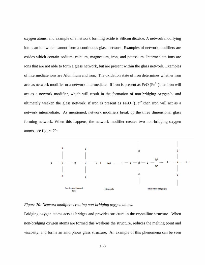
158

oxygen atoms, and example of a network forming oxide is Silicon dioxide. A network modifying

ion is an ion which cannot form a continuous glass network. Examples of network modifiers are

oxides which contain sodium, calcium, magnesium, iron, and potassium. Intermediate ions are

ions that are not able to form a glass network, but are present within the glass network. Examples

of intermediate ions are Aluminum and iron. The oxidation state of iron determines whether iron

acts as network modifier or a network intermediate. If iron is present as FeO (Fe2+

)then iron will

act as a network modifier, which will result in the formation of non-bridging oxygen’s, and

ultimately weaken the glass network; if iron is present as Fe2O3 (Fe3+

)then iron will act as a

network intermediate. As mentioned, network modifiers break up the three dimensional glass

forming network. When this happens, the network modifier creates two non-bridging oxygen

atoms, see figure 70:

Figure 70: Network modifiers creating non-bridging oxygen atoms.

Bridging oxygen atoms acts as bridges and provides structure in the crystalline structure. When

non-bridging oxygen atoms are formed this weakens the structure, reduces the melting point and

viscosity, and forms an amorphous glass structure. An example of this phenomena can be seen

159

in Figure 70 where sodium is acting as the network modifier. Sodium contributes to the non-

bridging oxygen atoms and balances the charge. When the viscosity is reduced, a liquid phase is

formed and sticking between particles build up resulting in agglomeration formation. The

sticking phenomena, can be described by a Frenkel’s sintering model. This sintering model

relates viscous flow sintering to the rate of coalescence of particles in terms of physical

properties such as viscosity, surface tension and particle size. Frenkel’s sintering model is:

Where x is the radius of growth between spherical particles, with radius r, η is the viscosity, γ is

the surface tension and t is the time. The sintering phenomena between particles are depicted in

Figure 71:

Figure 71: Viscous flow sintering of particles. (Benson, Sondreal 2010)

160

The liquid phase is formed when network modifiers weaken the crystalline structure and

decreases the viscosity. Surface tension, similar to viscosity, decreases with an increase in

temperature. Raask describes decrease in surface tension by relating it to endothermic

dehydration of water present in clays, mainly, Kaolinite, Montmorillonite, and Illite. These clays

lose the water that is present in them which causes destruction of the crystal lattice structure. The

change in shape of their crystal lattice structure, upon heating, decreases the surface tension and

forces the particles to take on a spherical shape, which will also increase sintering (Raask, 1985).

The main mechanism of ash deposit strength is by viscous flow, which is described by Raask as:

The growth and strength of the deposit are directly related to the amount of liquid and inversely

proportional to the viscosity. The sintering due to viscous liquid phase occurs when the liquid on

each particle exerts a surface tension force, which pulls the particles together (Benson, Sondreal

2010). The viscosity is inversely proportional to the sintering rate, which implies that the lower

the viscosity the more sintering will occur. Equally important, as temperature increases both

viscosity and surface tension decrease. The viscosity of the North Dakota lignite was calculated

using the Kalmanovitch-Urbain Model Figure 72:

161

Figure 72: Viscosity prediction of lignite using Kalmanovitch viscosity prediction model.

The Kalmanovitch viscosity model is a modified Urbain model for predicting viscosity behavior.

The Urbain derived model is based on the known behavior of network formers and modifiers,

specifically SiO2, Al2O3, TiO2, Fe2O3, CaO, MgO,K2O,Na2O (Laumb, Benson Katrinak). The

data is taken from the ash analysis of the lignite, Table 38.

0.00

1.00

2.00

3.00

4.00

5.00

700 800 900 1000 1100 1200 1300

Vis

cosi

ty, L

og 1

0 p

ois

e

Temperature (°C)

Kalmanovitch Viscosity Prediction Model

162

Table 14: ASTM mineral analysis of coal.

Analysis of Ash Oxide basis

(wt%)

Silicon Dioxide (SiO2) 19.23

Aluminum Oxide

(Al2O3) 9.2

Titanium Dioxide (TiO2) 0.33

Iron Oxide (Fe2O3) 7.33

Calcium Oxide (CaO) 19.64

Magnesium Oxide

(MgO) 5.07

Potassium Oxide (K2O) 0.79

Sodium Oxide (Na2O) 10.75

SO3 23.65

P2O5 0.12

Strontium Oxide (SrO) 0.54

Barium Oxide (BaO) 0.47

Manganese (MnO2) 0.1

163

Figure 73: Viscosity calculations of unclassified point count data.

And the viscosity is calculated at the operating temperature of 750 ° C, the results of those

viscosity calculations can be seen in Figure 73. The viscosity was also calculated for the

unclassified material in each the SEM point count data, and can be seen in figure 73. Based on

figure 73, the majority of the impurities are forming deposits 2.5 and 3.5 log10 poise. This is the

region where strong deposits form. At the operating temperature of 750 °C the agglomerate

samples are well in the sintering and fusing and melting region. The mineral analysis of lignite

can be seen in table 38 as it can be seen there is a high amount of alkali and alkaline earth metals,

sodium and calcium. Based on the theory and literature presented the alkali and alkaline earth

0

1

2

3

4

5

6

7

700 800 900 1000 1100 1200 1300

Vis

cosi

ty lo

g 10

(po

ise

)

Temperature (° C)

Viscosity of unclassified point count data

1-1C

1-1 F

1 2 - 1

2-6A

2-9A

Molten Liquid

Sintering

T250

Growth/Shedding

Growth-Removable

Fusing/Melting

Strong deposits

164

elements along with iron will cause the formation of low melting point phases will be the cause

particle bonding, sintering and agglomeration formation.

Numerous agglomeration samples were prepared and analyzed under different conditions

using the SEM. Regardless of what conditions the agglomerates were formed under, there were

similar trends in their chemical composition. The morphological analysis consistently showed

calcium, silicon, aluminum, sodium and iron as the most significant components. The

morphology results for the air gasification (Figures 47,48,52) experiments, showed similar trends

where calcium was the most abundant network modifier, with silicon and aluminum being the

next two most abundant network formers. The point count analysis for the air gasification sample

showed a lot of unclassified material glass materials that were rich in calcium (Table 19).

Based on the analysis of the agglomerates, the alkali and alkaline earth metals, both

sodium and calcium play a prominent role in agglomeration formation. This data, agrees with

past data and the literature, which indicates that lower ranked coals, such as high sodium North

Dakota lignite that contain a high amount of alkali and alkaline earth metals will cause

operational problems for gasification systems. For fluidized bed systems these operational

problems appear in the form of agglomerates, which if left unchecked can cause a decrease the

quality of fluidization, which indirectly affects syngas quality, and ultimately defluidization.

The ash composition of the lignite used in these tests, Table 38, shows a high level of glass

formers with 19% silica, and an even larger amount of network modifiers in calcium 19% and

sodium at 10%. Figure 72 shows the viscosity of lignite ash at different temperatures. Based at

the operating temperature of 750 °C the corresponding viscosity is high at 3.5 log(pois). In this

165

temperature range, based on the Kalmanovitch model, the viscosity is prone to sintering. The

data suggests that the sintering is due to viscous flow offered by Frenkel’s sintering model.

Based on the CCSEM analysis of the mineral grains present in the lignite coal, Table 39

there are significant amounts of quartz, pyrite, and clay (kaolinite, illite, and montmorillonite)

present in the coal matrix; these minerals along with the organically associate elements have the

potential to produce the bonding phases responsible for the sintering.

166

Table 15: CCSEM analysis of Center lignite coal.

Particle size range, µm 1 to 2.2

2.2 to

4.6 4.6 to 10 10 to 22 22 to 46

46 to

400 Totals

QUARTZ 0.4 3.6 9.2 8.3 2.2 0.4 24.1

IRON OXIDE 0 0 0.4 0.9 0 0 1.3

PERICLASE 0 0 0 0 0 0 0

RUTILE 0.1 0 0 0.3 0 0 0.4

ALUMINA 0 0 0 0 0 0 0

CALCITE 0.2 0.1 1.3 0.5 0.2 0 2.2

DOLOMITE 0 0.2 0.1 0 0 0 0.3

ANKERITE 0 0 0 0 0 0 0

KAOLINITE 0.1 1.1 1.6 2.1 0.2 0.1 5.2

MONTMORILLONITE 0.1 0.1 0.8 0.6 0 0 1.6

K AL-SILICATE(Illite) 0.1 1.6 1.5 1 0.2 0.2 4.6

FE AL-SILICATE 0 0.4 0.6 0.3 0 0 1.3

CA AL-SILICATE 0.2 0.5 0.6 1 0 0 2.3

NA AL-SILICATE 0 0.1 0.3 0 0 0 0.5

ALUMINOSILICATE 0 0.5 1.7 0.5 0.1 0 2.8

MIXED AL-SILICA 0.1 0 0.5 0.4 0 0 1

FE SILICATE 0 0 0 0 0 0 0

CA SILICATE 0 0 0.3 0.1 0 0 0.4

CA ALUMINATE 0 0 0 0 0 0 0

PYRITE 0.5 3.4 8.1 10.9 4.6 1 28.5

PYRRHOTITE 0 0 0 0 0.4 0 0.4

OXIDIZED PYRRHO 0 0 0 0 0 0 0

GYPSUM 0 0 0.1 0 0 0 0.1

BARITE 0 0.3 0.8 0.2 0.2 0 1.5

APATITE 0.1 0 0 0 0 0 0.1

CA AL-P 0 0 0 0 0 0 0

KCL 0 0 0 0 0 0 0

GYPSUM/BARITE 0 0 0 0 0 0 0

GYPSUM/AL-SILIC 0 0 0.7 0 0 0 0.7

SI-RICH 0.1 0.4 4.1 2.8 0.4 0.4 8.1

CA-RICH 0.1 0.1 0.1 0 0 0 0.3

CA-SI RICH 0 0 0 0 0 0 0

UNKNOWN 0.5 1.7 5.2 3.5 0.6 0.6 12.2

TOTALS 2.6 14.2 37.7 33.7 9.2 2.7 100

167

The data shows a large amount of iron in addition to calcium and sodium in the morphology

analysis. The iron, which reacts with silicates and aluminosilicates lowers the melting point, and

initiates the formation of viscous liquid flow and sintering. This along with the calcium and

sodium released from the organically associated coal matrix, act as network modifiers which

breaks up the silicate structure and forms low viscosity glass. Glass or amorphous phase

formation in these agglomerates is prevalent. It should be noted that the agglomeration formed

under combustion conditions were generated at an operating temperature of 850 °C. Combustion

experiments were performed first and at both 750 °C and 850 °C. Due to the problems faced at

the higher temperature all experiments performed after the combustion experiments were

performed at 750 °C, no agglomerates formed under combustion conditions at the lower

temperature. On the contrary, the agglomerations formed under gasification conditions were all

generated at a temperature of 750 °C. This observation coincides with ideas set forth by

Kalmanovitch as well as other investigators that the reaction of iron in the reduced form will

react with silicates to produce liquids at lower temperature as compared to iron in a higher

oxidation state that is present in oxidizing atmospheres than in reducing atmospheres. This will

lead to a greater sintering potential in reducing atmosphere versus an oxidizing atmosphere

(Kalmanovitch, Miller 1988).

5.6 Summary

Gasification experiments were performed under both air-blown and oxygen-blown

conditions. For each set of experiments for both air and oxygen blown, the syngas

composition was recorded and averaged over time and plotted against changing conditions.

Confidence intervals were calculated and found that all the data fell within the confidence

168

interval, this was performed to validate the accuracy of the data. A mass balance was

performed on each experiment to calculate the overall carbon conversion of the system. The

cold gas efficiency was also calculated based on the syngas composition. The syngas

composition, as well as carbon conversion and cold gas efficiency were compared to the

literature values. During the course of the experiments, agglomerates were generated and

collected. These samples were prepared and analyzed using microscopy techniques. The

agglomerates were analyzed using morphology for their elemental composition, and point

count analysis for their mineral composition.

169

6. CHAPTER VI

7. Conclusion

The primary objective of this project was to design, construct, and commission a

bench scale fluidized bed reactor with lignite coal as the design fuel and to generate and study

behavior of fuel associated impurities under selected combustion and gasification conditions.

The design of fluidized bed was based on empirical correlations, fluidization and combustion

calculations and computer software simulation. The basis of the design was centered on the

minimum fluidization velocity. The fluidization and combustion calculations were checked

against a computer simulation to verify their validity. The reactor was then built and

commissioned. A number of combustion and gasification experiments were performed using a

highly reactive lignite coal from North Dakota. The results showed that the fluidized bed reactor

could be operated over a range of coal, oxygen, air, and steam flow rates. Combustion

experiments were done with air and oxygen. Carbon conversion efficiencies over 90% were

achieved. Gasification testing was conducted under air and oxygen blown and with steam only.

The system was tested for its ability to optimize syngas composition in both air and oxygen

blown conditions. Two sets of experiments, air and oxygen gasification were performed and

investigated. From these experiments the carbon conversion increased as the oxygen to carbon

ratio increased. Oxygen blow gasification compared to air blown gasification oxygen blown

gasification; oxygen blown gasification has a higher output capacity, generating a lot more

hydrogen than in air gasification. This also correlates to a higher quality syngas, which can be

seen in the cold gas efficiencies. This is a result of no

170

nitrogen being present in oxygen gasification. Without nitrogen diluting the syngas, the

hydrogen, carbon dioxide, and carbon monoxide were the most abundant and is higher quality

syngas. A hydrogen rich syngas of 54% was able to be produced. The high amount of hydrogen

produced is due to the water gas shift reaction that takes place downstream of the reactor. There

is a significant temperature drop between where the reactor is produced and where the syngas is

analyzed. The data was compared to and coincided with the literature, which further validates the

system. Bed agglomeration caused by the reaction of impurities present in the lignite with bed

particles was found to occur in both combustion and gasification conditions. The agglomerates

produced in the fluidized bed reactor were examined using scanning electron microscopy to

determine some of the bonding materials that contribute to agglomerate formation.. Based on the

analysis of the impurity generated agglomerates it was found that they mainly consisted of silica,

calcium and sodium. The mechanism by which these agglomerates formed was through the

sintering of the alkali and alkaline earth metal impurities that are present in lignite and are

typically responsible for problems in coal gasification systems. To conclude, it was possible to

build a bench scale fluidized bed reactor that was capable of producing realistic syngas

composition and realistic impurities, and the problems associate with it, to further study and

advance gasification research.

171

8. Recommendations for Future Work

There are several modifications that can be made to improve the system operability and

performance that may depend on the application of interest. The system is very flexible and can

be operated over a range of conditions. Therefore it will be up to the operator to decide how the

fluidized bed can be used to advance current research goals. For this work the fluidized bed was

designed and optimized to produce hydrogen. However, in the experimental section, other

applications were briefly explored to show the versatility of the fluidized bed system. Besides air

and oxygen gasification to produce hydrogen, the two other applications that were explored were

oxygen fired combustion and steam hydro-gasification for retort systems. To improve the system

in its current state, some modifications need to be implemented and further experiments should

be performed. Further experiments which need to be performed mainly deal with the fluidized

bed itself. One of the main attractions of fluidized bed technology is its ability to use low ranked

coals, which are in high abundance, as fuel sources. However one of the main issues with the

utilization of lignite is its impurities, which get released and form agglomerates. These

agglomerates cause operational problems. Experiments should be performed by either adding

materials such as Kaolinite or bauxite to the bed. These are two materials which have shown to

mitigate agglomeration formation, by preventing the network modifiers (Na, Ca, Fe2+

, and K)

that react with network formers (silicates) producing low viscosity liquid phases. The network

modifiers that come from the coal creating non-bridging oxygen atoms in the silicates that result

in more mobile structure that decreases melting points and viscosities. The kaolinite or bauxite

materials react with the network modifiers instead, which create a higher melting point material,

preventing liquid formation, bonding, and sintering. These two materials, as well as others

172

should be investigated. Next, the bed height of the fluidized should be investigated to see how

the bed height affects the syngas, as well as hydrogen production. Initially a bed height was to

be varied for optimization coal throughput. However, experiments at one bed height were

performed and experiments focused on changing other operating parameters. The experiments

conducted as part of this thesis were performed with what is considered a deep fluid bed, where

the aspect ratio of the bed is greater than one. After analyzing the data, the actual throughput of

coal was lower than the theoretical values. As a result, the preliminary calculations and testing

indicate that a reduction in bed height will allow for both a smoother fluidization, as well as a

higher throughput of coal through the reactor. A range of 0.5 to 0.9 kg/hr of coal throughput,

compared to the theoretical 0.9 to 1.3 kg/hr. Based on these preliminary results two more sets of

experiments should be conducted to verify the preliminary calculations. One set of experiments

should be performed where the bed is close to unity, this calculation was performed in the design

chapter. And another set of experiments should be performed with a shallow bed. These

experiments would confirm that a reduced bed height would produce a higher quality syngas,

while enhancing the capacity of coal through the reactor. In order to make the fluidized bed

more practical, experiments need to be performed with different fuels. In this work the design

fuel was lignite. Fluidized beds are best suited for low ranked coals, because the chemistry of

these coals, they are more reactive than high ranked coals. Since fluidized beds need to operate at

a lower temperature to prevent ash from forming the in the bed, the high reactivity of lower

ranked coals compensates for the lower operating temperatures. Different ranked coals have

different chemistries associated with them and therefore carry their own unique set of problems

when trying to utilize them as a fuel source for fluidized gasification. Experiments should be

173

performed using both bituminous and subbituminous coal to see how these fuels behave in the

system, and what quality of syngas is produced. The fluidized bed system can be used for

different applications. One possible application is to perform research chemical looping.

Modifications would have to be made to the system. Chemical looping can use coal to produce

hydrogen or using oxygen combustion to generate a concentration of carbon dioxide in the

product gas. Based on the systems capability to perform oxygen-carrier testing, as well as

product gas that is high in hydrogen, chemical looping would be a good application for this

system. Due to the fact that chemical looping uses to fluidized beds, not only would a second

fluidized need to be constructed but the current one would have to be made into a circulating

fluidized bed. Changing the system from a bubbling fluidized bed to a circulating fluidized

would also allow for research in more diverse applications. At the University of North Dakota

the fluidized bed system is in close proximity to drop tube furnace that is used for combustion

studies. Regardless of which application the fluidized bed will be used to study future work

needs to be focusing on improving the control of the system through automation. The laser gas

analyzer recorded data every thirty seconds, which allowed for a lot of reliable data to be

collected efficiently. Implementation of data recording software needs to be employed for

temperature and pressure of the system. When experiments were performed, temperature

profiles of the bed were recorded by hand. This made it more difficult to have a precise

knowledge of what is going on when interpreting data. More important then automatically

recording the temperature is recording and controlling the pressure drop across the fluidized bed.

Monitoring the pressure in the fluidized bed would give insight to the operator on how the

reactor is behaving and if there are any problems. If pressure transducers were implemented, it

174

would detect more subtle pressure changes which would allow for more a more smooth operation

and give the operator some foresight to any potential problems forming inside the bed. The

ability to monitor and record pressure electronically will allow for greater insight into research

problems like agglomeration formation.

175

9. Appendix A: Standard Operating Procedure for the fluidized bed gasifier

Shakedown Checklist:

Wear proper eye safety glasses and gloves at all times

Ensure system is clean and ready for experiments

Cyclone and condensers are cleaned

Bed material is in the reactor

Coal and additives are in the coal feeder.

Pressure leak test Performed

Insulation is on

Heat tapes are on

Water valve is opened

All necessary units are operational and on including:

Compressors

Air heater

Steam generator

Reactor heaters

Laser gas analyzer

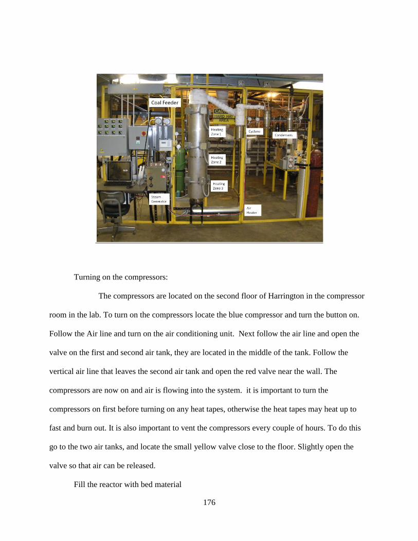
176

Turning on the compressors:

The compressors are located on the second floor of Harrington in the compressor

room in the lab. To turn on the compressors locate the blue compressor and turn the button on.

Follow the Air line and turn on the air conditioning unit. Next follow the air line and open the

valve on the first and second air tank, they are located in the middle of the tank. Follow the

vertical air line that leaves the second air tank and open the red valve near the wall. The

compressors are now on and air is flowing into the system. it is important to turn the

compressors on first before turning on any heat tapes, otherwise the heat tapes may heat up to

fast and burn out. It is also important to vent the compressors every couple of hours. To do this

go to the two air tanks, and locate the small yellow valve close to the floor. Slightly open the

valve so that air can be released.

Fill the reactor with bed material

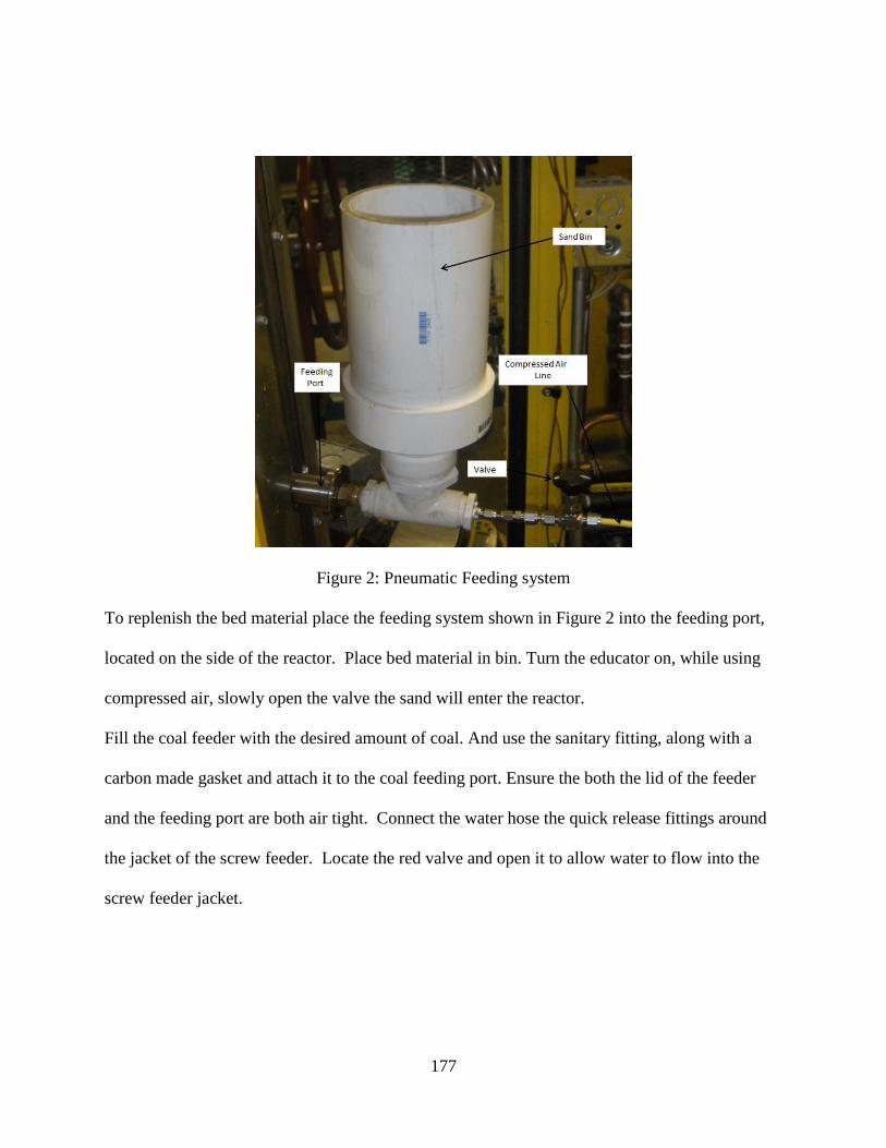
177

Figure 2: Pneumatic Feeding system

To replenish the bed material place the feeding system shown in Figure 2 into the feeding port,

located on the side of the reactor. Place bed material in bin. Turn the educator on, while using

compressed air, slowly open the valve the sand will enter the reactor.

Fill the coal feeder with the desired amount of coal. And use the sanitary fitting, along with a

carbon made gasket and attach it to the coal feeding port. Ensure the both the lid of the feeder

and the feeding port are both air tight. Connect the water hose the quick release fittings around

the jacket of the screw feeder. Locate the red valve and open it to allow water to flow into the

screw feeder jacket.

178

Figure 3: Coal feeding system

Please refer to the calibration curves for coal feed rates. It is important not to feed in coal until

the desired operating temperature is reached.

Perform Pressure leak test:

Run air through system and close the valve at the top let the pressure build up and observe the

pressure gauge, if the pressure does not hold or does not follow the trend below. First listen for

air leaking in the system. Check for leaks both audibly and visually. then take soapy water or

window cleaner and spray all of the fittings

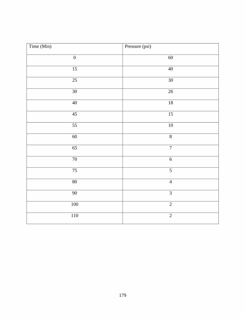
179

Time (Min) Pressure (psi)

0 60

15 40

25 30

30 26

40 18

45 15

55 10

60 8

65 7

70 6

75 5

80 4

90 3

100 2

110 2

180

Once the pressure test is complete, apply heat tape around product gas line and wrap with

insulation. Release the valve that was closed to perform the pressure leak test. Now that the bed

material is in the reactor, the coal feeder has coal in it and the pressure leak has been performed,

operation preparation can be performed.

Operation Preparation:

Reactor heaters:

Turn on the control panel located above the monitor by pressing the yellow button. Locate the

controls labeled outside top, middle and bottom. These are the controllers that control the heat to

the reactor. The inside top, middle and bottom are read only thermocouples. The controls display

the set point temperature at the bottom and operational temperature at the top. To change the

temperature press and hold the star button and press the up or down arrow. The controllers do

have a feature where it can automatically increase the temperature to the desired set point at a pre

determined rate, this feature is called ramp/soak. To use this feature from the SPrr in level 1

press and hold the star button and use the up/down arrow to the desired ramp rate. A ramp rate of

y = 66.368e-0.034x R² = 0.9941

0

10

20

30

40

50

60

0 20 40 60 80 100 120

Pre

ssu

re (

Psi

)

Time (min)

Pressure Leak Rate

181

250 to 300 °C/hr was used for the experiments. The soak feature allows for the temperature to be

held at the set point for a desired amount of time, then automatically ramp back down. If the

soak feature is not implemented then the heaters will stay at the set point indefinitely or until it is

manually ramped down. Note if power is lost in ramp mode, once power is restored, the ramp

will restart.

Air Pre-heater:

Turn on air pre-heater and set the target temperature. (Note it is important to have air flowing

before turning on any heating elements) this temperature can be monitored with an independent

thermocouple reader. At low flowrates the temperature may not be able to reach its desired set

point.

Steam Generator:

Turn the steam generator on by pressing the red button. It will build pressure up to around 30-35

psi. open the yellow valve this will allow steam to flow. The steam flowrate is controlled by a

black valve located right after the yellow valve. Please refer to the calibration curve. It is also

important to vent the steam generator to clean out any dirt that builds up in there. Before using it

go behind the unit and locate a red blow down valve near the floor. Open that valve to release

any dirt build up.

Laser gas analyzer

Make sure the laser gas analyzer is on, and check the filter to see if it needs maintenance.

There are additional filters that also need to be checked on the sample line before performing any

experiments. Perform a calibration each time before performing any experiments.

Turn all heat tapes to the desired temperatures.

182

Experiments can be performed at this point, once the reactor and the heat tapes have reached the

desired set point.

Procedure for operating the fluidized bed as a combustor:

With the air flowing through the reactor, feed in coal at a low flowrate. Observe the laser gas

analyzer for changes in oxygen and carbon dioxide. Slowly increase the amount of fuel into the

reactor once there is indication of combustion occurring.

Procedure for operating the fluidized bed as a gasifier:

In order to operate the fluidized bed as a gasifier. It is practiced that it always be ran in

combustion mode at the beginning and end of each experiment. Get the reactor to a steady state

combustion condition. Once it is there maintain the overall flowrate of that steady state

condition. To switch to gasification mode. Cut back on the amount of oxidant and replaced the

amount reduced with steam, such that the overall flowrate is the same. Continue to decrease the

oxidant while replacing it with steam. Observe the laser gas analyzer for gasification condtions.

Sampling:

Ash/Char sampling:

If a sample of ash or char is desired. It can be done without disrupting operation. To do

this the bypass valve needs to be implemented. To do this first open the bypass valve. This will

divert the product gas away from the cyclone. Right after that has been opened close the valve

downstream. increase the amount of air on the educator, this will allow for a sample to be taken

without the product gas getting in the way. Once the two valves have been implemented take a

part the sanitary fitting that connects the ash can to the cyclone. Take a sample, clean out the ash

183

can and connect back to the cyclone. Open the valve downstream then close the bypass valve.

See Figure 4

Figure 4: sampling system for ash and char.

Bed material sample:

If a sample of the bed is desired for analysis, it is recommended to wait until the sand has

cooled. Taking a hot sand sample is dangerous and it could potentially melt the container. In

order to eject the sand from the bed the valve used for the pressure test needs to be closed. Turn

the air on high. With a pair of wrenches, open the discharge port at the bottom of the reactor.

Hold a container to collect the sand as it comes out of the reactor.

184

Cleaning the system after experimentation:

Once everything is turned off, the system can be cleaned for the next run. In order to do this all

the downstream equipment needs to be taken apart. It may be necessary to dismantle the top

flange of the reactor, if that is off Interest. To dismantle the downstream equipment, use a

wrench and loosen the fittings, starting at the end and working backwards, towards the reactor.

First release the sanitary fitting on the last condenser to remove the baffle inside. These baffles

are spring loaded so be cautious when dismantling them. Once the baffle is removed proceed to

do the remove the baffle from the other condenser. Once those are removed. The insulation

around the product gas line can be removed and then dismantled. Proceed to remove the fittings

from the cyclone. Now that the two condensers and the cyclone are removed, they can be washed

with soap and water with a wire brush to remove and build up. Once the units and the product

gas line is cleaned it can be reassembled for the next experiment.

Removing the reactor from the heaters/base plate:

With the cyclone removed, remove the insulation and the heat tape. Using 1 and 1/8 inch

wrench loosen the bolts in an alternating pattern to remove the flange (this will protect the flange

gasket from damage). Remove the bottom bolts in the same fashion. Open up the clamshell

heaters by unscrewing the bolts on the side, this will allow the clamshell case to open up. Lift the

reactor by placing a firm grip on the sand discharge port and lift the reactor up to remove it from

the stand.

Placing and securing the reactor in the clamshell case.

1. Place the distributor plate FRIT on the bottom flange, which sits in the black ring stand.

2. Place the gasket over the frit and make sure it’s centered.

185

3. Place the reactor on the bottom flange; by lining up the coal feed inlet tube with the

opening in heating vestibules. The bottom flange should line up with the flange at the

bottom of the reactor. (Note: it is important when placing the reactor on the black ring

stand not to move the frit out of position.)

4. Using a 1 and 1/8 inch wrench, bolt down the reactor to the bottom of the flange. Make

sure when tightening the bolts to tighten them in a star pattern. By tightening the bolts in

a star pattern, this will allow pressure to be evenly distributed along the gasket and

prevent it from getting damaged. Bolting down the bolts in a star pattern can be achieved

by placing 4 bolts in the flange, one bolt in every other hole. Tighten the bolts on

opposite sides of each other until all 4 bolts are tightened. Proceed to secure the reactor

with the remaining four bolts in the same fashion.

5. Place the top flange, with the pipe attached to it, through the bolts on the top of the

reactor.

6. Attach the pipe side that is attached to the top flange to the cyclone, via a sanitary fitting.

Make sure there is a high temperature gasket in between the connection.

7. Using a 9/16” wrench, attach the ¼” Swagelok nut to the top flange.

8. Coat the top bolts with anti-seize and bolt down the top flange in the same star pattern as

the bottom flange.

9. Using a 7/16” wrench, unscrew the Swagelok caps on the top of the reactor and insert the

thermocouples into the reactor. Make sure to tighten them down and plug them in to the

corresponding plug.

10. The reactor is now set up

186

10. Appendix B: Loss on Ignition Tables

187

11. Appendix C: Temperature profiles of the reactor for gasification experiments.

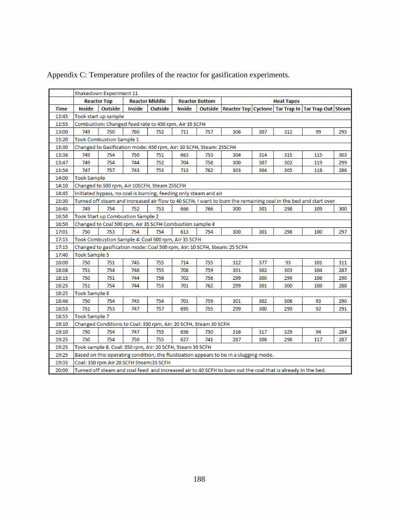
188

Appendix C: Temperature profiles of the reactor for gasification experiments.

189

Appendix C: Temperature profiles of the reactor for gasification experiments.

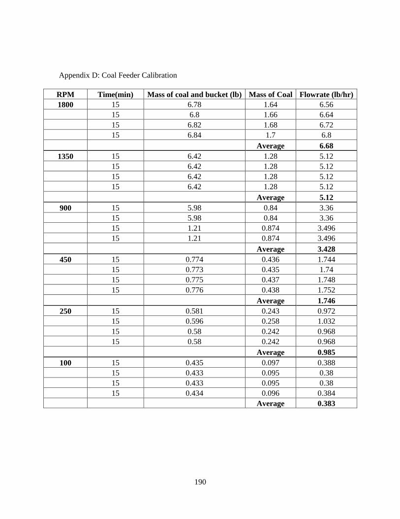
190

12. Appendix D: Coal Feeder Calibration

RPM Time(min) Mass of coal and bucket (lb) Mass of Coal Flowrate (lb/hr)

1800 15 6.78 1.64 6.56

15 6.8 1.66 6.64

15 6.82 1.68 6.72

15 6.84 1.7 6.8

Average 6.68

1350 15 6.42 1.28 5.12

15 6.42 1.28 5.12

15 6.42 1.28 5.12

15 6.42 1.28 5.12

Average 5.12

900 15 5.98 0.84 3.36

15 5.98 0.84 3.36

15 1.21 0.874 3.496

15 1.21 0.874 3.496

Average 3.428

450 15 0.774 0.436 1.744

15 0.773 0.435 1.74

15 0.775 0.437 1.748

15 0.776 0.438 1.752

Average 1.746

250 15 0.581 0.243 0.972

15 0.596 0.258 1.032

15 0.58 0.242 0.968

15 0.58 0.242 0.968

Average 0.985

100 15 0.435 0.097 0.388

15 0.433 0.095 0.38

15 0.433 0.095 0.38

15 0.434 0.096 0.384

Average 0.383

191

y = 268.35x - 10.299 R² = 0.9997

0

200

400

600

800

1000

1200

1400

1600

1800

0 1 2 3 4 5 6 7

Re

volu

tio

ns

pe

r m

inu

te (

rpm

)

Coal Feed Rate (lbs/hr)

Calibration of Lignite (40 mesh)

192


1800 15 1.868 1.53 6.12

15 1.917 1.579 6.316

15 1.918 1.58 6.32

15 1.92 1.582 6.328

Average 6.271

1350 15 1.544 1.206 4.824

15 1.55 1.212 4.848

15 1.551 1.213 4.852

15 1.553 1.215 4.86

Average 4.846

900 15 1.155 0.817 3.268

15 1.155 0.817 3.268

15 1.168 0.83 3.32

15 1.079 0.741 2.964

Average 3.205

450 15 0.456 0.118 0.472

15 0.673 0.335 1.34

15 0.499 0.161 0.644

15 0.398 0.06 0.24

Average 0.674

250 15 0.564 0.226 0.904

15 0.378 0.04 0.16

15 0.43 0.092 0.368

15 0.344 0.006 0.024

Average 0.364

193


120 15 0.438 0.1 0.4

15 0.447 0.109 0.436

15 0.448 0.11 0.44

15 0.448 0.11 0.44

Average 0.429

110 15 0.438 0.1 0.4

15 0.438 0.1 0.4

15 0.438 0.1 0.4

15 0.438 0.1 0.4

Average 0.4

100 15 0.418 0.08 0.32

15 0.429 0.091 0.364

15 0.429 0.091 0.364

15 0.43 0.092 0.368

Average 0.354

90 15 0.418 0.08 0.32

15 0.418 0.08 0.32

15 0.421 0.083 0.332

15 0.421 0.083 0.332

Average 0.326

y = 246.08x + 194.04 R² = 0.9868

0

200

400

600

800

1000

1200

1400

1600

1800

2000

0 1 2 3 4 5 6 7

Re

volu

tio

ns

Pe

r M

inu

te (

RP

M)

Feed Rate (lbs/hr)

Calibration Of Lignite

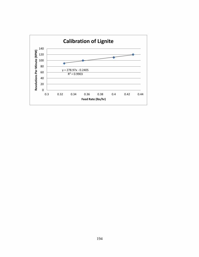
194

y = 278.97x - 0.2405 R² = 0.9903

0

20

40

60

80

100

120

140

0.3 0.32 0.34 0.36 0.38 0.4 0.42 0.44

Re

volu

tio

ns

Pe

r M

inu

te (

RP

M)

Feed Rate (lbs/hr)

Calibration of Lignite

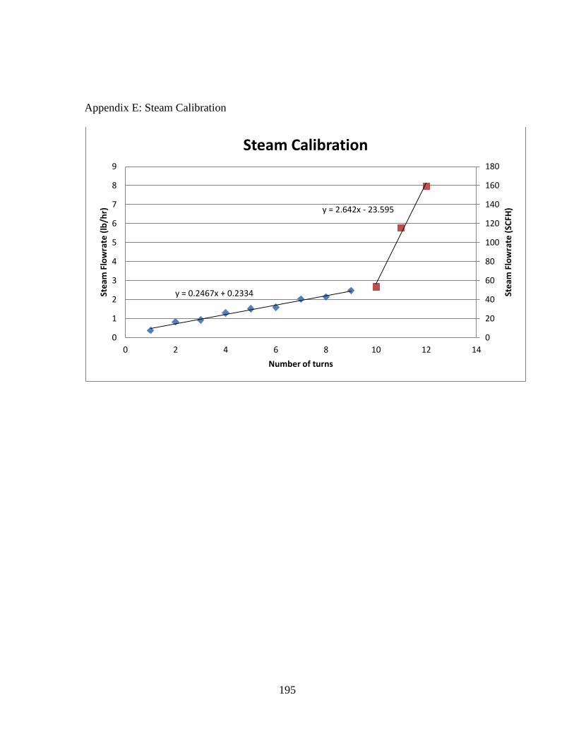
195

13. Appendix E: Steam Calibration

y = 0.2467x + 0.2334

y = 2.642x - 23.595

0

20

40

60

80

100

120

140

160

180

0

1

2

3

4

5

6

7

8

9

0 2 4 6 8 10 12 14

Ste

am F

low

rate

(SC

FH)

Ste

am F

low

rate

(lb

/hr)

Number of turns

Steam Calibration

196

14. Appendix F: Syngas of hydrogen sulfide for oxygen gasification experiments.

0

0.1

0.2

0.3

0.4

0.5

0.6

0.7

0.5 1 1.5 2 2.5 3

Hyd

roge

n S

ulf

ide

Co

nce

ntr

atio

n (

Vo

l %)

C/O

Air Blown Gasification

197

15. Appendix G:Fuel properties of lignite: Ultimate, Proximate and Mineral analysis

Mineral Analysis of Ash Dry basis

(wt%)

Silicon Dioxide (SiO2) 19.23

Aluminum Oxide (Al2O3) 9.2

Titanium Dioxide (TiO2) 0.33

Iron Oxide (Fe2O3) 7.33

Calcium Oxide (CaO) 19.64

Magnesium Oxide (MgO) 5.07

Potassium Oxide (K2O) 0.79

Sodium Oxide (Na2O) 10.75

SO3 23.65

P2O5 0.12

Strontium Oxide (SrO) 0.54

Barium Oxide (BaO) 0.47

Manganese (MnO2) 0.1

Proximate Analysis As Received (wt%

) Dry basis

(wt%)

Total Moisture 31.2

Ash 6.38 9.27

Volatile Matter 28.82 41.89

Fixed Carbon 33.6 48.84

Total Sulfur 0.65 0.94

Ultimate Analysis As Received (wt%

) Dry basis

(wt%)

Total Moisture 31.2

Ash 6.38 9.27

Carbon 47.83 69.52

Hydrogen 6.67 4.62

Nitrogen 0.52 0.76

Total Sulfur 0.65 0.94

Oxygen by Difference 37.95 14.89

Chlorine (μg/g) 31.6 45.9

Heating Value (BTU/lb) 7526 10939

198

References

Agglomeration Behavior in a bubbling fluidized bed at high temperature. Chem.Eng.Comm.

191:1329-1342 (2004).

Analyses, C., Ash, C., Fluorescence, B. X., Coupled, I., Mass, P., Atomic, F., & Spectrometry,

A. (2009). Standard Test Methods for Loss on Ignition ( LOI ) of Solid Combustion

Residues 1.

Annual Energy Outlook 2011. (2011) (Vol. 0383).

Aspen Properties User Guide. (n.d.).

Barsin, J.A.Mineral Matter And Ash Deposition from Coal.”Fouling &Slagging In Commercial

Equipment Due to High Sodium Coals.” Feb -26 1988.

Barrett, R. E. (n.d.). Slagging and Fouling Due to Impurities in Combustion Gasses.”Utilization

of Fouling/Slagging/Corrosive Low-Ranked Coals—New Developments in South

Australia.”. In United Engineering Trustees inc.

Barrett, R. E. . (n.d.). Slagging and Fouling Due to Impurities in Combustion Gasses

“Comparison of Low-Rank Coal Ash Sintering Characteristics With Pilot Plant Fouling

Tendencies. In United Engineering Trustees inc.

Bartels, M., Lin, W., Nijenhuis, J., Kapteijn, F., & van Ommen, J. R. (2008). Agglomeration in

fluidized beds at high temperatures: Mechanisms, detection and prevention. Progress in

Energy and Combustion Science, 34(5), 633–666. doi:10.1016/j.pecs.2008.04.002

Benson, S. (n.d.). Fuels Technology Notes Spring 2012.

Benson, S. A. (1985). Performance of Low-Rank Coal in Atmospheric Fluidized Bed

Combustion. Grand Forks.

Benson, S. A., & Sondreal, E. A. (n.d.). GASIFICATION OF LIGNITES OF NORTH

AMERICA SUMMARY REPORT BY :, (August 2010).

Berkowitz, N. (1979). An Introduction to Coal Technology. Academic Press.

BI,H.T., Grace, J.R. Flow Regime Diagrams for Gas-Solid fluidization and Upward Transport.

International journal of fluidized flow 21 No 6 pg 1229-1238, 1995

199

C. Higman. (2013). State of the Gasification Industry – the Updated Worldwide Gasification

Database.

C. Higman, V. B. (2003). Gasification. Gulf Professional Publishing.

Chmielniak, T., & Sciazko, M. (2003). Co-gasification of biomass and coal for methanol

synthesis. Applied Energy, 74(3-4), 393–403. doi:10.1016/S0306-2619(02)00184-8

Collot, A. (2006). Matching Gasification Technologies to Coal Properties. International Journal

of Coal Geology, 65, 195–212.

Cooper, C. David Alley, F. (2010). Air Pollution Control a Design Approach (4th ed.).

Curtis, J., Rao, A. The Effect of Column Diameter and Bed Height on Minimum Fluidization

Velocity. AICHE Journal 56 No 9 September 2010

Description, B. (n.d.). Dosing: Single Screw Feeder with Agitation.

Fluidized Bed Technology-Overview” (office of fossil energy, U.S. Department of Energy,

Washington, DC,2007);

Gavin Towler, R. S. (2008). Chemical Engineering Design Principles, Practice, and Economics

of Plant Design. Butterworth-Heinemann.

Geldart, D. Gas Fluidization Technology. John Wiley & Sons. 1986

Govind, R. Shah, J. (n.d.). Modeling and simulation of an Entrained flow coal Gasifier. AIChE

Journal, 30(1).

Helble, J.J.; Mojtahedi, W.; Lyyranen, J.; Jokiniemi, J.; Kauppinen, E. Trace Element

Partitioning During Coal Gasification. Fuel 1996, 75, 931-939.

Impurities in Combustion and Gasification Systems Lecture # 14 – Section 2 . Fireside behavior

I – Transport Mechanisms Section 3 -- Fireside behavior of fuel impurities – slagging and

fouling. (n.d.).

Impurities in Combustion and Gasification Systems Lecture t # 10 – Mechanisms M h i of f

impurity transformations II – coalescence and fragmentation Section 2 -- Transformations

of Impurities in. (n.d.).

Industry, A., & Paper, W. (2012). Gasification Process Modeling.

Konemann, J. W. (2009). OLGA Tar Removal Technology.

200

Kunii, D., & Levenspiel, O. (1991). Fluidization engineering (2nd ed.). Butterworth-Heinemann.

Retrieved from http://www.lavoisier.fr/livre/notice.asp?ouvrage=1289154

Laumb, J. Benson, S.A. Coal Quality and Boiler Operations: Viscosity Predictions.

Lawson, E. (2001). Modern Statistics for Engineering and Quality Improvement.

Lin, C. Wey, M. Lu, C. Prediction of defluidization time of alkali composition at various

operating conditions during incineration. Powder technology 161 (2006) 150-157 Lind, T. et al.

The Impact of ash deposition on coal fired plants. Proceedings of the Engineering Foundation

Conference. “Alkali Metal Behavior In Atmospheric Circulating Fluidized Bed Coal

Combustion.” June

Lind, T. et al. The Impact of ash deposition on coal fired plants. Proceedings of the Engineering

Foundation Conference. “Characteristics of Ash Particles from Pressurized Fluidized Bed

Gasification.” June

Manzoori, A.R. Role of the Inorganic Matter in Agglomeration and Defluidization during the

Circulating Fluid Bed Combustion of Low Rank Coals. Department of Chemical Engineering,

the University of Adelaide, Australia, 1990.

Matsuoka, K., Suzuki, Y., Eylands, K., Benson, S., & Tomita, a. (2006). CCSEM study of ash

forming reactions during lignite gasification. Fuel, 85(17-18), 2371–2376.

doi:10.1016/j.fuel.2006.05.014

Maurstad, O., Herzog, H., Bolland, O., & Beér, J. (n.d.). Impact of coal quality and gasifier

technology on IGCC performance, 1–6.

Meuzelaar, H. (1992). Advances in Coal Spectroscopy.

Miller, S.F. Kalmanovitch, D.P. Relation of Slag and Surface Tension to Sintering Potential.

ACS Conference: Ash Chemistry Coal, Toronto, Canada 32:2 June 5-10 1988

Minchener, A. J. (2005). Coal gasification for advanced power generation. Fuel, 84(17), 2222–

2235. doi:10.1016/j.fuel.2005.08.035

N, G. (n.d.). ME 545-Fluidized-bed combustion engineering lecture notes.

NETL.doe.gov. (n.d.).

201

Oleschko, H. Schimrosczyk A. Lippert, H. Müller, M. Influence of coal composition on the

release of Na-, K-, Cl-, and S-species during the combustion of brown coal. Fuel 86 (2007)

2275-2282

Pain, C., Mansoorzadeh, S., Oliveiera, C.R.E. A Study of Bubbling and Slugging Fluidized Beds

Using the Two-Fluid Granular Temperature Model. International journal of multiphase flow 27

527-551, 2001.

Piestsch, W. Size Enlargement by Agglomeration. John Wiley & Sons 1991

P. Basu. (2006). Combustion and Gasification in Fluidized Beds. Hemisphere Publishing

Corporation.

Powell, C.; Morreale, B. (2008). Materials Challenges in Advanced Coal Conversion

Technologies. MRS Bulletin 33. No 4., 309–315.

Pugsley, T. Mahinpey, N. (n.d.). A Review of Fluidized Bed Gasification Technology May 3-6

2010 Dresden, Germany. In 4th International Freiburg Conference on IGCC & XtL

Technologies.

Raask, E. (1985). Mineral Impurites In Coal Combustion Behavior, Problems, and Remedial

Measures. Hemisphere Publishing Corporation

Ramirez, J.J.,Martinez,J.D.,Petro,S.L. Basic Design of a fluidized Bed Gasifier for Rice Husk on

a Pilot Scale. Latin American Applied Research. 37 299-306, 2007

Rao, A., Curtis, J. S., Hancock, B. C., & Wassgren, C. (2010). The Effect of Column Diameter

and Bed Height on Minimum Fluidization Velocity, 56(9). doi:10.1002/aic

Singer Joseph .Combustion Fossil Power Systems 3rd

edition 1981

Song, W. Et el.Prediction of Temperature of Critical Viscosity for Coal Ash Slag. AICHE

Journal 57 no 10 Oct 2011.

Souza-Santos, M. L. de. (2010). Solid Fuels Combustion and Gasification Modeling, Simulation,

and Equipment Operations (2nd ed.). Taylor& Francis.

Technology, A. (n.d.). Aspen Plus Getting Started Modeling Processes with Solids.

The Coal Resource- A Comprehensive Overview of Coal. (2005). In World Coal Institute,

Richmond-upon-Thames.

202

The Future of Coal-Options for a Carbon-Constrained World. (n.d.). Retrieved from

http://web.mit.edu/coal

Thiel, W., Potter, O. Slugging In Fluidized Beds. Industrial Engineering 16 No 2 1977

Turns, S. R. (2012). An Introduction to Combustion Concepts and Applications (3rd ed.).

McGraw-Hill.

Weber, S. Et el. Predicting agglomerate fragmentation and agglomerate material survival in

fluidized beds. Powder Technology. 210 (2001) 87-102

Weber, S. et el. Agglomerate stability in fluidized beds of glass beads and silica sand. Powder

Technology 165 (2006) 115-127.

Wen-Ching Yang. (2003). Handbook of Fluidization and Fluid-Particle Systems. Marcel Dekker.

West, S.S, Williamson, J. Laughlin, M.K. The Impact of ash deposition on coal fired plants.

Proceedings of the Engineering Foundation Conference. “Mineral Interactions During Fluidized

Bed gasification of Coals” June 1993

World Energy Council. (2013) (pp. 1–32).

Zenz, F. Fluidization and Fluid-Particle Systems. Reinhold Publishing Corporation 1960

Zhang, D Jackson, P Vuthaluru, H. (n.d.). Impact of Mineral Impurities in Solid Fuel Com-

bustion. “Low-Rank Coal and Advanced Power Technologies For Power Generation.” In

Engineering Foundation Conference on Mineral Matter November.

design and construction of a fluidized bed

Documents