design and control of hydronic radiant cooling systemsescholarship.org/uc/item/6qc4p0fr.pdf ·...

UC BerkeleyHVAC Systems

TitleDesign and Control of Hydronic Radiant Cooling Systems

Permalinkhttps://escholarship.org/uc/item/6qc4p0fr

AuthorFeng, Jingjuan (Dove)

Publication Date2014-04-01

eScholarship.org Powered by the California Digital LibraryUniversity of California

https://escholarship.org/uc/item/6qc4p0fr

https://escholarship.org

http://www.cdlib.org/

Design and Control of Hydronic Radiant Cooling Systems

By

Jingjuan Feng

A dissertation submitted in partial satisfaction of the

requirements for the degree of

Doctor of Philosophy

in

Architecture

in the

Graduate Division

of the

University of California, Berkeley

Committee in charge:

Professor Stefano Schiavon, Chair

Professor Gail Brager

Professor Edward Arens

Professor Francesco Borrelli

Spring 2014

PhD Dissertation, Dept. of Architecture, UC Berkeley 2014



© 2014

By Jingjuan Feng



1

ABSTRACT


by

Jingjuan Feng

Doctor of Philosophy in Architecture

University of California, Berkeley

Professor Stefano Schiavon, Chair

Improving energy efficiency in the Heating Ventilation and Air conditioning (HVAC) systems in buildings is critical to achieve the energy reduction in the building sector, which consumes 41% of all primary energy produced in the United States, and was responsible for nearly half of U.S. CO2 emissions. Based on a report by the New Building Institute (NBI), when HVAC systems are used, about half of the zero net energy (ZNE) buildings report using a radiant cooling/heating system, often in conjunction with ground source heat pumps. Radiant systems differ from air systems in the main heat transfer mechanism used to remove heat from a space, and in their control characteristics when responding to changes in control signals and room thermal conditions. This dissertation investigates three related design and control topics: cooling load calculations, cooling capacity estimation, and control for the heavyweight radiant systems. These three issues are fundamental to the development of accurate design/modeling tools, relevant performance testing methods, and ultimately the realization of the potential energy benefits of radiant systems.

Cooling load calculations are a crucial step in designing any HVAC system. In the current standards, cooling load is defined and calculated independent of HVAC system type. In this dissertation, I present research evidence that sensible zone cooling loads for radiant systems are different from cooling loads for traditional air systems. Energy simulations, in EnergyPlus, and laboratory experiments were conducted to investigate the heat transfer dynamics in spaces conditioned by radiant and air systems. The results show that the magnitude of the cooling load difference between the two systems ranges from 7-85%, and radiant systems remove heat faster than air systems. For the experimental tested conditions, 75-82% of total heat gain was removed by radiant system during the period when the heater (simulating the heat gain) was on, while for air system, 61-63% were removed. From a heat transfer perspective, the differences are mainly because the chilled surfaces directly remove part of the radiant heat gains from a zone, thereby bypassing the time-delay effect caused by the interaction of radiant heat gain with non-active thermal mass in air systems. The major conclusions based on these findings are: 1) there are important limitations in the definition of cooling load for a mixing air system described in



2

Chapter 18 of ASHRAE Handbook of Fundamentals when applied to radiant systems; 2) due to the obvious mismatch between how radiant heat transfer is handled in traditional cooling load calculation methods compared to its central role in radiant cooling systems, this dissertation provides improvements for the current cooling load calculation method based on the Heat Balance procedure. The Radiant Time Series method is not appropriate for radiant system applications. The findings also directly apply to the selection of space heat transfer modeling algorithms that are part of all energy modeling software.

Cooling capacity estimation is another critical step in a design project. The above mentioned findings and a review of the existing methods indicates that current radiant system cooling capacity estimation methods fail to take into account incident shortwave radiation generated by solar and lighting in the calculation process. This causes a significant underestimation (up to 150% for some instances) of floor cooling capacity when solar load is dominant. Building performance simulations were conducted to verify this hypothesis and quantify the impacts of solar for different design scenarios. A new simplified method was proposed to improve the predictability of the method described in ISO 11855 when solar radiation is present.

The dissertation also compares the energy and comfort benefits of the model-based predictive control (MPC) method with a fine-tuned heuristic control method when applied to a heavyweight embedded surface system. A first order dynamic model of a radiant slab system was developed for implementation in model predictive controllers. A calibrated EnergyPlus model of a typical office building in California was used as a testbed for the comparison. The results indicated that MPC is able to reduce the cooling tower energy consumption by 55% and pumping power consumption by 26%, while maintaining equivalent or even better thermal comfort conditions.

In summary, the dissertation work has: (1) provided clear evidence that the fundamental heat transfer mechanisms differ between radiant and air systems. These findings have important implications for the development of accurate and reliable design and energy simulation tools; (2) developed practical design methods and guidance to aid practicing engineers who are designing radiant systems; and (3) outlined future research and design tools need to advance the state-of-knowledge and design and operating guidelines for radiant systems.



i

Table of Contents

Design and Control of Hydronic Radiant Cooling Systems ................................................................... 1 ABSTRACT ........................................................................................................................................... 1 Table of Contents .................................................................................................................................... i List of Figures ........................................................................................................................................ v List of Tables ....................................................................................................................................... viii List of Symbols ..................................................................................................................................... ix Acknowledgement ............................................................................................................................... xiii 1 INTRODUCTION .......................................................................................................................... 1

1.1 The challenges for HVAC systems ................................................................................. 1 1.2 Hydronic radiant systems ................................................................................................ 2

1.2.1 System types ............................................................................................................ 4 1.2.2 Applications in high performance buildings............................................................ 6

1.3 The Radiant system design process and its challenges .................................................... 6 1.3.1 Cooling load analysis method ................................................................................. 9 1.3.2 Radiant system capacity estimation ....................................................................... 10 1.3.3 Control considerations ........................................................................................... 11

1.4 Research objectives ....................................................................................................... 13 1.5 Organization of the dissertation ..................................................................................... 14

2 BACKGROUND .......................................................................................................................... 16 2.1 The heat transfer theory ................................................................................................. 16

2.1.1 Heat transfer at radiant cooling surfaces ............................................................... 16 2.1.2 Heat transfer in the slab and with the water side ................................................... 17

2.2 Design guidelines .......................................................................................................... 19 2.3 Cooling load analysis methods ...................................................................................... 23

2.3.1 Cooling load definitions ........................................................................................ 23 2.3.2 Calculation methods .............................................................................................. 24 2.3.3 Summary................................................................................................................ 28

2.4 Radiant system capacity evaluation methods ................................................................ 28 2.4.1 Heat transfer at radiant surface .............................................................................. 29 2.4.2 Cooling capacity estimation method ..................................................................... 32 2.4.3 Summary and questions ......................................................................................... 38

2.5 Control for thermally active building systems .............................................................. 38 2.5.1 Literature review ................................................................................................... 38



ii

2.5.2 Summary................................................................................................................ 40 2.6 State of art of the design industry .................................................................................. 40

2.6.1 Survey and interview ............................................................................................. 40 2.6.2 Case studies ........................................................................................................... 43 2.6.3 Summary................................................................................................................ 46

2.7 Conclusions ................................................................................................................... 47 3 COMPARISON OF COOLING LOADS BETWEEN RADIANT AND AIR SYSTEMS-----SIMULATION STUDY ....................................................................................................................... 48

3.1 Introduction ................................................................................................................... 48 3.1.1 Radiant vs. air systems .......................................................................................... 48 3.1.2 Cooling load at radiant surface and hydronic level ............................................... 48

3.2 Methodology and modelling approach .......................................................................... 49 3.2.1 Simulation Runs .................................................................................................... 50 3.2.2 Model Specifications ............................................................................................. 51 3.2.3 Parameters investigated ......................................................................................... 54

3.3 Results ........................................................................................................................... 54 3.3.1 24-hour total cooling energy.................................................................................. 55 3.3.2 Peak cooling rate ................................................................................................... 58

3.4 Discussion ..................................................................................................................... 61 3.4.1 Cooling load dynamics .......................................................................................... 61 3.4.2 Influencing factor .................................................................................................. 63

3.5 Summary ....................................................................................................................... 65 4 COMPARISON OF COOLING LOADS BETWEEN RADIANT AND AIR SYSTEMS-----EXPERIMENTAL COMPARISON .................................................................................................... 67

4.1 Introduction ................................................................................................................... 67 4.2 Methodology ................................................................................................................. 67

4.2.1 Experimental facilities and setup ........................................................................... 67 4.2.2 Measuring instruments and uncertainty ................................................................. 70 4.2.3 Uncertainties analysis ............................................................................................ 71 4.2.4 Uncertainty in airside cooling rate ......................................................................... 71 4.2.5 Uncertainty in radiant panel cooling rate .............................................................. 72 4.2.6 Test procedure ....................................................................................................... 72

4.3 Results ........................................................................................................................... 72 4.4 Discussion ..................................................................................................................... 77 4.5 Summary ....................................................................................................................... 77



iii

5 COOLING LOAD CALCULATION AND MODELING METHODS FOR RADIANT SYSTEMS-----APPLICATIONS ......................................................................................................... 79

5.1 Introduction ................................................................................................................... 79 5.1.1 Heat balance method ............................................................................................. 79 5.1.2 Radiant time series method ................................................................................... 80

5.2 Methodology ................................................................................................................. 81 5.3 Results ........................................................................................................................... 81 5.4 Discussion ..................................................................................................................... 82

5.4.1 Definition of cooling load for different radiant system types ................................ 82 5.4.2 Cooling load calculation procedure ....................................................................... 84 5.4.3 Impacts on space modeling method ....................................................................... 85 5.4.4 Proposed improvements in the design standards ................................................... 85

5.5 Summary ....................................................................................................................... 86 6 RADIANT FLOOR COOLING SYSTEM CAPACITY ESTIMATION WITH SOLAR LOAD ................................................................................................................................................... 88

6.1 Introduction ................................................................................................................... 88 6.2 Solar radiation in buildings ........................................................................................... 90

6.2.1 Modeling of solar radiation in buildings ............................................................... 90 6.2.2 Radiant cooling surface thermal response ............................................................. 91

6.3 Impact of solar heat gain on radiant floor cooling capacity .......................................... 92 6.3.1 Standardized cooling capacity methods ................................................................ 92 6.3.2 Methodology.......................................................................................................... 93 6.3.3 Results ................................................................................................................... 95

6.4 New simplified model for radiant floor cooling capacity estimation ............................ 97 6.5 Implications for sizing of associated air system ............................................................ 98 6.6 Conclusions ................................................................................................................. 102

7 CONTROL OF HEAVYWEIGH RADIANT SLAB SYSTEMS .............................................. 104 7.1 Introduction ................................................................................................................. 104 7.2 Model based predictive control (MPC) ....................................................................... 104 7.3 Methodology ............................................................................................................... 106 7.4 The case study building: David Brower Center (DBC) ............................................... 107 7.5 EnergyPlus Model ....................................................................................................... 108

7.5.1 Base model specifications ................................................................................... 109 7.5.2 Base model evaluation ......................................................................................... 109

7.6 Control methods .......................................................................................................... 113 7.6.1 Heuristic rule based control ................................................................................. 113



iv

7.6.2 Model predictive control ..................................................................................... 114 7.7 Comparison of control methods .................................................................................. 118

7.7.1 Thermal comfort .................................................................................................. 119 7.7.2 Energy consumption ............................................................................................ 120 7.7.3 Examples of MPC and heuristic control from the test ......................................... 120

7.8 Summary ..................................................................................................................... 122 8 CONCLUSIONS ........................................................................................................................ 124

8.1 Cooling load analysis .................................................................................................. 124 8.2 Radiant system capacity .............................................................................................. 126 8.3 Control of radiant slab systems ................................................................................... 127

9 REFERENCE ............................................................................................................................. 128 Appendix A: Derivation of correlation for calculating 𝒒𝒔𝒘_𝒔𝒐𝒍" ..................................................... 141 Appendix B: David Brower Center building modeling information .................................................. 143 Appendix C: Computing system states satisfying certainty equivalence ........................................... 147



v

List of Figures Figure 1-1: Examples of buildings with radiant systems installed ..................................... 6 Figure 1-2: Design process for radiant system in the context of whole building design .... 8 Figure 1-3: Heavyweight radiant slab systems are slow to respond to control signals .... 12 Figure 1-4: Thermal comfort in spaces conditioned by precooling radiant slabs for a representative summer day: Water supply temperature kept at 18 °C .............................. 13 Figure 2-1: Heat transfer balance at the radiant surface and hydronic loop ..................... 17 Figure 2-2: Thermal resistance representation of heat transfer in the slab and between the slab and water loop ........................................................................................................... 18 Figure 2-3: Differences between heat gain and cooling load due to thermal delay effect (modified based on ASHRAE HOF 2013) ....................................................................... 24 Figure 2-4: Cooling load diagram from ASHRAE Handbook – Fundamentals ............... 26 Figure 2-5: Radiant slab system design diagram example (Uponor 2010) ....................... 34 Figure 2-6 : Results for question 1: tools used for cooling load calculation (N = 22)...... 42 Figure 2-7: Results for question 2: cooling load used for sizing radiant slab system (N=14) ............................................................................................................................... 42 Figure 2-8: Results for question 3: tools/methods used for dimensioning radiant system (N = 15) ............................................................................................................................. 42 Figure 3-1: Isometric Base Case (Only G4-G6 have windows) ....................................... 52 Figure 3-2: Comparison of temperatures at the inside surface of exterior wall between radiant and air systems. (G6 typical ceiling: cl_shade_rad0.6) ........................................ 56 Figure 3-3: Range of 24-hour total energy percentage difference between air system and radiant system at surface level (left) and hydronic level (right) ....................................... 57 Figure 3-4: Comparison of design day cooling rate profiles between radiant and air systems. (G6 typical ceiling: cl_shade_rad0.6) ................................................................ 58 Figure 3-5: Range of peak cooling rate percentage difference between air system and radiant system at surface level (left) and hydronic level (right) ....................................... 60 Figure 3-6: Comparison of surface cooling breakdown (convective and radiative part) for Case rad0.6 in group 3: air system (left) and radiant cooling panel (RCP) system (right)62 Figure 3-7: Comparison of zone air temperatures, operative temperatures, active and non-active surface temperatures between radiant and air systems (G6 typical ceiling: cl_shade_rad0.6) ............................................................................................................... 63 Figure 3-8: Scatter plot of radiation ratio vs. 24 hour total cooling energy percentage difference at both surface (left) and hydronic (right) level ............................................... 64 Figure 3-9: Scatter plot of radiation ratio vs. design peak cooling load percentage difference at both surface (left) and hydronic (right) level ............................................... 64 Figure 4-1: The test chamber setup and sensor layout ...................................................... 68 Figure 4-2: (a) Radiant ceiling configured to have air diffuser in the middle for air system test, (b) floor heating mats on top of concrete boards, (c) porous feature of the heaters allowed heat transfer between concrete and the rest the room ......................................... 68 Figure 4-3: Test chamber sensor layout ............................................................................ 69 Figure 4-4: Comparison of operative temperatures between radiant and air system tests: (A) 1080 W test and (B) 1500 W test ............................................................................... 73



vi

Figure 4-5: Comparison of concrete and wall temperatures between radiant and air system tests: (A) 1080 W test and (B) 1500 W test .......................................................... 74 Figure 4-6: Comparison of measured instantaneous cooling rates for radiant and air systems: (A) 1080 W test and (B) 1500 W test ................................................................ 75 Figure 4-7: Percentage differences of measured instantaneous cooling rates for radiant and air systems, i.e. [(radiant cooling rate – air cooling rate )/ (air cooling rate)] %. : (A) 1080 W test and (B) 1500 W test ...................................................................................... 75 Figure 4-8: Profiles of accumulative heater energy input to chamber and accumulative energy removal by radiant and air systems: (A) 1080 W test and (B) 1500 W test ......... 76 Figure 4-9: Comparison of percentage of total heat gain being removed and percentage of energy storage for radiant and air systems during heater-on periods: (A) 1080 W test and (B) 1500 W test .......................................................................................................... 76 Figure 5-1: Schematic of the heat balance process in zone (ASHRAE HOF 2013 Chapter 18) ..................................................................................................................................... 80 Figure 5-2: Comparison of measured and predicted instantaneous cooling rates using heat balance (HB) method (A) and using radiant time series (RTS) method (B) for radiant and air systems: 1080 W test ................................................................................................... 82 Figure 5-3: The cooling load generation scheme for air system adapted from ASHRAE Fundamentals (2013) and proposed modifications for radiant system ............................. 84 Figure 6-1: Example of buildings with radiant floor cooling systems to remove soalr radiation. Left: Akron art museum, OH (image source: http://www.coop-himmelblau.at/architecture/projects/akron-art-museum); Right: Hearst tower lobby, New York (image source: http://www.getresponse.com/archive/adff/ADFF-NEWSLETTER-02_22_2012-8384159.html).............................................................................................. 89 Figure 6-2: schematic of the single zone model and the radiant floor systems simulated 94 Figure 6-3: Cooling design day floor radiation heat flux breakdown for the 864 simulation runs .................................................................................................................. 95 Figure 6-4: Comparison of radiation heat flux at radiant surface between EnergyPlus and ISO/ASHRAE method using box-plot of the 864 simulation runs ................................... 96 Figure 6-5: Comparison of simulated cooling capacity with cooling capacity calculated using ISO -11855 method (Eq.7-10) for system Type A-D: (A) with interior blind, i.e. no shortwave solar radiation; (B) without shade, i.e. with shortwave solar radiation. .......... 97 Figure 6-6: Zone operative temperature ranges during all simulation runs ...................... 99 Figure 6-7: Comparison of EnergyPlus simulated capacity and predicted capacity using proposed method and ISO method. ................................................................................. 100 Figure 6-8: Example of how enhanced cooling capacity impact sizing of air system .... 101 Figure 6-9: Example of using the proposed method for sizing of air system ................. 101 Figure 6-10: Comparison of EnergyPlus simulated air system size and predicted air system size if proposed and ISO method are used for estimating radiant floor system capacity. .......................................................................................................................... 102 Figure 7-1: Receding Horizon Idea (source:(Borrelli et al. 2010)) ................................ 105 Figure 7-2: case study building: David Brower Center, Berkeley, CA (Source: Tim Griffith) ........................................................................................................................... 108 Figure 7-3: Radiant slab with under floor air distribution (UFAD) system ................... 108 Figure 7-4: Typical floor plan of DBC building and radiant system zoning .................. 109



vii

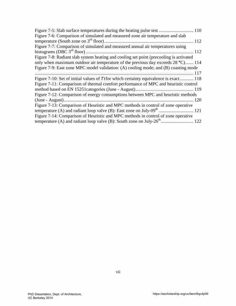
Figure 7-5: Slab surface temperatures during the heating pulse test .............................. 110 Figure 7-6: Comparison of simulated and measured zone air temperature and slab temperature (South zone on 3rd floor) ............................................................................. 112 Figure 7-7: Comparison of simulated and measured annual air temperatures using histograms (DBC 3rd floor) ............................................................................................. 112 Figure 7-8: Radiant slab system heating and cooling set point (precooling is activated only when maximum outdoor air temperature of the previous day exceeds 28 °C) ....... 114 Figure 7-9: East zone MPC model validation: (A) cooling mode; and (B) coasting mode......................................................................................................................................... 117 Figure 7-10: Set of initial values of 𝑇𝑡𝑡for which certainty equivalence is exact ............ 118 Figure 7-11: Comparison of thermal comfort performance of MPC and heuristic control method based on EN 15251catogories (June - August) .................................................. 119 Figure 7-12: Comparison of energy consumptions between MPC and heuristic methods (June - August) ................................................................................................................ 120 Figure 7-13: Comparison of Heuristic and MPC methods in control of zone operative temperature (A) and radiant loop valve (B): East zone on July-09th .............................. 121 Figure 7-14: Comparison of Heuristic and MPC methods in control of zone operative temperature (A) and radiant loop valve (B): South zone on July-26th ............................ 122



viii

List of Tables

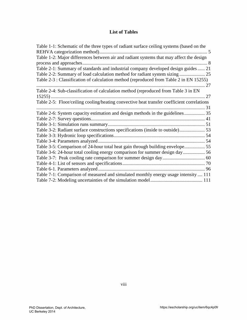
Table 1-1: Schematic of the three types of radiant surface ceiling systems (based on the REHVA categorization method) ......................................................................................... 5 Table 1-2: Major differences between air and radiant systems that may affect the design process and approaches ....................................................................................................... 8 Table 2-1: Summary of standards and industrial company developed design guides ...... 21 Table 2-2: Summary of load calculation method for radiant system sizing ..................... 25 Table 2-3 : Classification of calculation method (reproduced from Table 2 in EN 15255)........................................................................................................................................... 27 Table 2-4: Sub-classification of calculation method (reproduced from Table 3 in EN 15255) ............................................................................................................................... 27 Table 2-5: Floor/ceiling cooling/heating convective heat transfer coefficient correlations........................................................................................................................................... 31 Table 2-6: System capacity estimation and design methods in the guidelines ................. 35 Table 2-7: Survey questions.............................................................................................. 41 Table 3-1: Simulation runs summary ................................................................................ 51 Table 3-2: Radiant surface constructions specifications (inside to outside) ..................... 53 Table 3-3: Hydronic loop specifications ........................................................................... 54 Table 3-4: Parameters analyzed ........................................................................................ 54 Table 3-5: Comparison of 24-hour total heat gain through building envelope ................. 55 Table 3-6: 24-hour total cooling energy comparison for summer design day .................. 56 Table 3-7: Peak cooling rate comparison for summer design day ................................... 60 Table 4-1: List of sensors and specifications .................................................................... 70 Table 6-1. Parameters analyzed ........................................................................................ 96 Table 7-1: Comparison of measured and simulated monthly energy usage intensity .... 111 Table 7-2: Modeling uncertainties of the simulation model ........................................... 111



ix

List of Symbols 𝐴𝑈𝑆𝑇 Area-weighted temperature of all indoor surfaces of walls, ceiling, floor,

window, doors, etc. (excluding active cooling surfaces), ℃.

𝐴𝑟𝑠 Surface area in contact between room and slab, m2

𝐴𝑟𝑎,𝑖 Surface area in contact between room and zone i, m2

𝐶𝑝 Specific heat capacity of air, J/kg·K

𝐶𝑝,𝑤 Specific heat capacity of water, J/kg·K

𝐶𝑝,𝑠 Specific heat capacity of slab, J/kg·K

D Diameter of water pipe in slab, m

𝐺𝑠 Radiation generated in or incident on the room, W

ℎ𝑐 Convective heat transfer coefficient, W/m2.K

ℎ𝑟𝑎𝑑 Linear radiant heat transfer coefficient, W/m2.K

ℎ𝑡𝑜𝑡 Combined convection and radiation heat transfer coefficient, W/m2.K

𝐾 Lumped thermal resistance between hydronic loop and space, W/m2·K

K H, floor Lumped thermal resistance between hydronic loop and space for floor heating, W/m2·K

L Total length of water pipe in slab, m

LWRR

The longwave radiation ratio, is defined as the ratio of simulated longwave radiation heat flux at the cooling surface to the radiation calculated using either ISO and ASHRAE methods

𝑚𝑎 Mass of air in room, kg

��𝑎𝑖𝑛 Mass flow rate of air into the room, kg/s

��𝑤𝑖𝑛 Mass flow rate of water into the slab, kg/s

𝑚𝑠 Mass of slab, kg

n Constant

𝑃𝑃𝑠𝑢𝑟𝑓,𝑝𝑘 Percentage difference of surface peak cooling rate between radiant and air system, %

𝑃𝑃ℎ𝑦𝑑,𝑝𝑘 Percentage difference of hydronic peak cooling rate between radiant and air system, %

𝑃𝑃𝑠𝑢𝑟𝑓,𝑡𝑜𝑡 Percentage difference of surface level 24-hour total cooling energy between radiant and air system, %

𝑃𝑃ℎ𝑦𝑑,𝑡𝑜𝑡 Percentage difference of hydronic level level 24-hour total cooling between radiant and air system, %



x

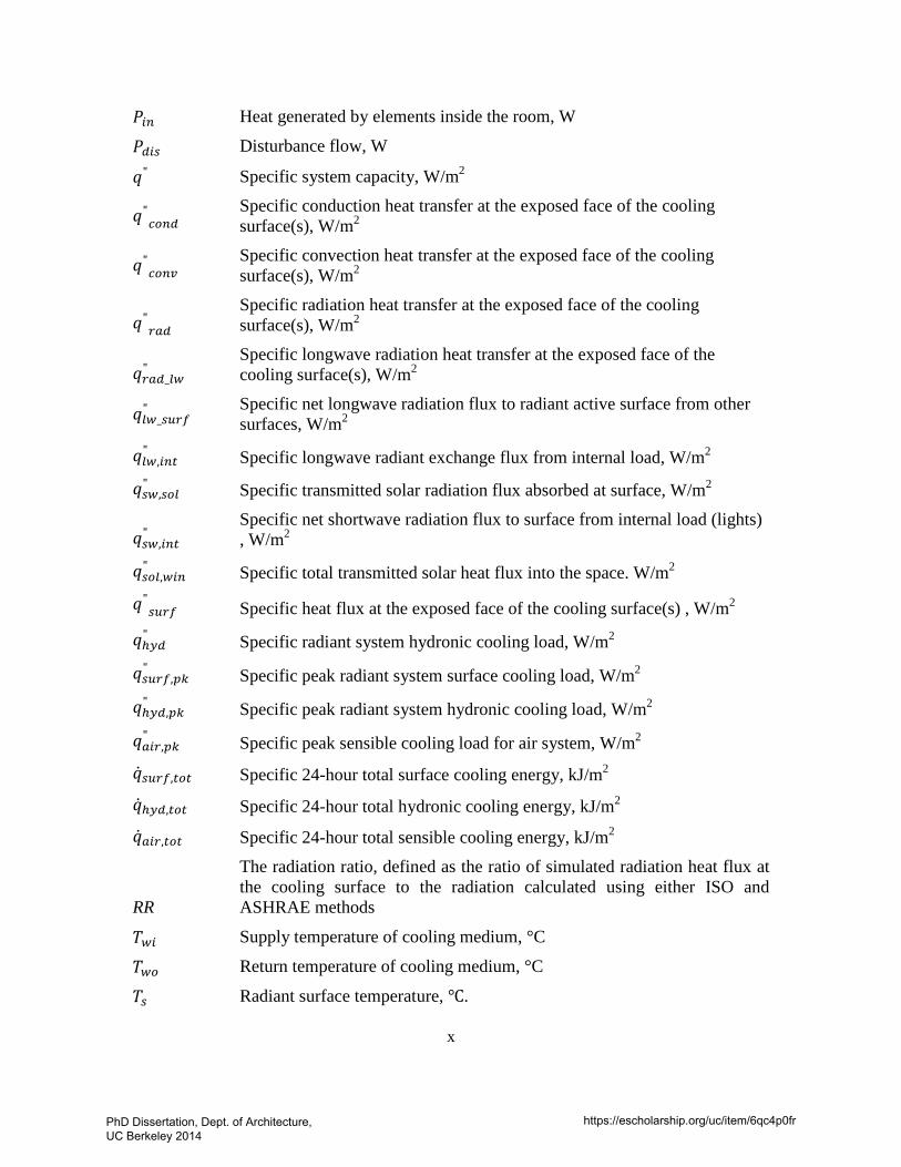
𝑃𝑃𝑖𝑛 Heat generated by elements inside the room, W

𝑃𝑃𝑑𝑖𝑠 Disturbance flow, W

𝑞𝑞" Specific system capacity, W/m2

𝑞𝑞"𝑐𝑜𝑛𝑑 Specific conduction heat transfer at the exposed face of the cooling

surface(s), W/m2

𝑞𝑞"𝑐𝑜𝑛𝑣 Specific convection heat transfer at the exposed face of the cooling

surface(s), W/m2

𝑞𝑞"𝑟𝑎𝑑

Specific radiation heat transfer at the exposed face of the cooling surface(s), W/m2

𝑞𝑞𝑟𝑎𝑑_𝑙𝑤"

Specific longwave radiation heat transfer at the exposed face of the cooling surface(s), W/m2

𝑞𝑞𝑙𝑤_𝑠𝑢𝑟𝑓" Specific net longwave radiation flux to radiant active surface from other

surfaces, W/m2

𝑞𝑞𝑙𝑤,𝑖𝑛𝑡" Specific longwave radiant exchange flux from internal load, W/m2

𝑞𝑞𝑠𝑤,𝑠𝑜𝑙" Specific transmitted solar radiation flux absorbed at surface, W/m2

𝑞𝑞𝑠𝑤,𝑖𝑛𝑡"

Specific net shortwave radiation flux to surface from internal load (lights) , W/m2

𝑞𝑞𝑠𝑜𝑙,𝑤𝑖𝑛" Specific total transmitted solar heat flux into the space. W/m2

𝑞𝑞"𝑠𝑢𝑟𝑓 Specific heat flux at the exposed face of the cooling surface(s) , W/m2

𝑞𝑞ℎ𝑦𝑑" Specific radiant system hydronic cooling load, W/m2

𝑞𝑞𝑠𝑢𝑟𝑓,𝑝𝑘" Specific peak radiant system surface cooling load, W/m2

𝑞𝑞ℎ𝑦𝑑,𝑝𝑘" Specific peak radiant system hydronic cooling load, W/m2

𝑞𝑞𝑎𝑖𝑟,𝑝𝑘" Specific peak sensible cooling load for air system, W/m2

��𝑞𝑠𝑢𝑟𝑓,𝑡𝑜𝑡 Specific 24-hour total surface cooling energy, kJ/m2

��𝑞ℎ𝑦𝑑,𝑡𝑜𝑡 Specific 24-hour total hydronic cooling energy, kJ/m2

��𝑞𝑎𝑖𝑟,𝑡𝑜𝑡 Specific 24-hour total sensible cooling energy, kJ/m2

RR

The radiation ratio, defined as the ratio of simulated radiation heat flux at the cooling surface to the radiation calculated using either ISO and ASHRAE methods

𝑇𝑤𝑖 Supply temperature of cooling medium, °C

𝑇𝑤𝑜 Return temperature of cooling medium, °C

𝑇𝑠 Radiant surface temperature, ℃.



xi

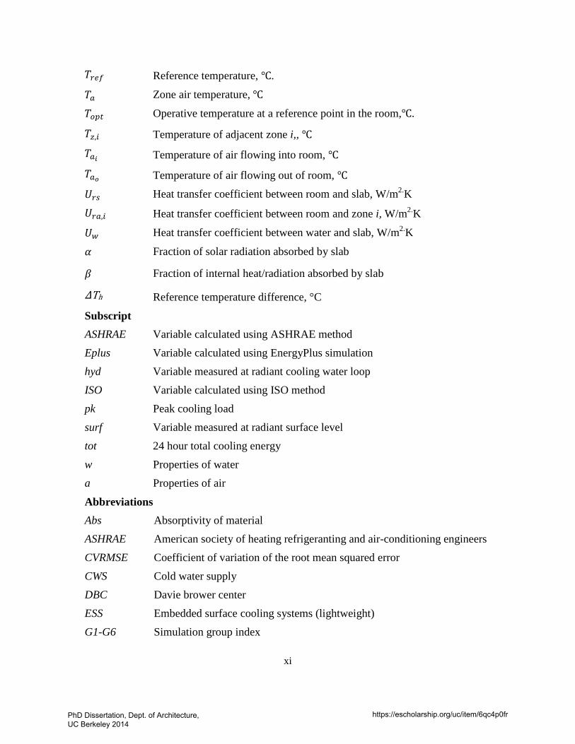
𝑇𝑟𝑒𝑓 Reference temperature, ℃.

𝑇𝑎 Zone air temperature, ℃

𝑇𝑜𝑝𝑡 Operative temperature at a reference point in the room,℃.

𝑇𝑧,𝑖 Temperature of adjacent zone i,, ℃

𝑇𝑎𝑖 Temperature of air flowing into room, ℃

𝑇𝑎𝑜 Temperature of air flowing out of room, ℃

𝑈𝑟𝑠 Heat transfer coefficient between room and slab, W/m2.K

𝑈𝑟𝑎,𝑖 Heat transfer coefficient between room and zone i, W/m2.K

𝑈𝑤 Heat transfer coefficient between water and slab, W/m2.K

𝛼 Fraction of solar radiation absorbed by slab

𝛽 Fraction of internal heat/radiation absorbed by slab

ΔTh Reference temperature difference, °C

Subscript ASHRAE Variable calculated using ASHRAE method

Eplus Variable calculated using EnergyPlus simulation

hyd Variable measured at radiant cooling water loop

ISO Variable calculated using ISO method

pk Peak cooling load

surf Variable measured at radiant surface level

tot 24 hour total cooling energy

w Properties of water

a Properties of air

Abbreviations Abs Absorptivity of material

ASHRAE American society of heating refrigeranting and air-conditioning engineers

CVRMSE Coefficient of variation of the root mean squared error

CWS Cold water supply

DBC Davie brower center

ESS Embedded surface cooling systems (lightweight)

G1-G6 Simulation group index



xii

HB Heat balance method

HVAC Heating ventilation and air conditioning system

LEED Leadership in Energy & Environmental Design

MPC Model predictive control(ler)

NMBE normalized mean bias error

SHGC Solar heat gain coefficient

RCP Radiant cooling panels

RTS Radiant time series

RTD Resistance Temperature Detector

TABS Thermally activated building systems

WWR Window to wall ratio



xiii

Acknowledgement

Completion of this dissertation was possible with the constant support and encouragement from many individuals.

First and foremost, I am greatly indebted to Professor Stefano Schiavon for his encouragement and guidance throughout my PhD candidature. He always devoted a great amount of time to carefully review of my papers, provide motivating and inspiring advices, and was willing to help me with many challenges I faced, even when they were unrelated to dissertation. I would also like to thank my committee members: Dr. Gail Brager for providing me continuous support and guidance during my whole PhD study; Dr. Edward Arens for his insightful comments that improved the dissertation; and Dr. Francesco Borrelli for opening my eyes up to the power of advanced control optimization technique and for his review of this part of the dissertation.

I am also especially grateful to my direct supervisor at the Center for the Build Environment, Fred Bauman, for his vision and leadership with the research project that leads to this dissertation work. As my day to day advisor, he patiently reviewed all my writings, provided valuable advices for improving my presentation skill, arranged and accompanied me to Winnipeg for the experiment, and send me encouraging message when I struggled and frustrated. I am also indebted to the entire Building Science Group for many insightful conversations, celebrations, tasty food, and restorative outings.

I would also like to express my appreciation to Brad Tully and Tom Epp of Price Industries for the use of their Hydronic Test Chamber in Winnipeg, and their effort in assisting with setting up the experiment. The experiment is a significant part of the study, and it would not have been possible without their help.

Last but not the least, I would like to acknowledge the support of my family: thanks to my husband Xiufeng Pang for his love, patience and many wise suggestion along the journey, our lovely daughter Faye for bringing me laugh every day; my parents and parents in law for providing endless help.

This PhD study was supported by the California Energy Commission (CEC) Public Interest Energy Research (PIER) Buildings Program. Partial funding was also provided by the Center for the Built Environment, University of California, Berkeley.



1

1 INTRODUCTION

1.1 The challenges for HVAC systems Policy makers, scientists, and engineers have paid increasing attention on how to address energy efficiency issues due to concerns about global warming and energy independency (Creyts 2007, APS 2008, Glicksman 2008). The building sector, according to the U.S. Energy Information Administration (EIA), consumed 41% of all primary energy produced in the United States, and was responsible for nearly half of U.S. CO2 emissions (EIA 2012). Several organizations have established ambitious goals for the efficiency level of future buildings. The American Institute of Architects issued “The 2030 Challenge” asking the global architecture and building community to adopt a series of greenhouse gas reduction targets for new and renovated buildings. Inspired by this, the California Energy Commission adjusted Title 24, the energy efficiency portion of the building codes, to require net-zero-energy performance in residential buildings by 2020 and in commercial buildings by 2030. Later, the Department of Energy also joined the effort by launching the Net Zero Energy Commercial Building Initiative. Heating, ventilation and air conditioning (HVAC) systems are becoming increasingly important for achieving those goals as they consume more than 40% of energy use in buildings and have significant impact on indoor air quality, thermal comfort and, consequently, the occupant’s quality of life (Fisk 2000, Clements-Croome 2006, EIA 2012). The goal is to provide an optimal indoor environment at low energy. However, for the last forty years, there have been no “disruptive breakthroughs” in the HVAC system performance, as theoretical and practical limitations inherent in the traditional air based HVAC systems impede radical improvements. First, transporting heat within buildings contributes to a significant share of HVAC energy consumption. One effective method of reducing this energy is through the reduction of the volumetric flow rate of the heat transfer fluid. The invention of the variable air volume (VAV) operating strategy was based on this principle. However, as a heat transfer fluid, air possesses low density and specific heat capacity, thus requiring a large volumetric flow rate to deliver the same amount of energy compared to using a heat carrier, such as water, with high density (832 times higher than air) and specific heat ( 4000 times higher than air).

The second energy inefficiency in HVAC design occurs during the heat exchange process between the distribution and conversion system (central plants). With conventional air systems, the surface area of heat exchangers, usually cooling/heating coils, is strictly limited by space and cost. Thus the central plants need to provide a high temperature source for heating and a cold temperature source for cooling. In most applications, chillers/boilers are used as the cooling/heating source. From the second law of thermodynamic perspective, chillers, operating based on a reversed Carnot cycle, would have a higher coefficient of performance (COP) with higher evaporating (heat source side) temperature and lower condensing (heat sink side) temperature. This means generating cold water at higher temperatures would improve chiller efficiency (ASHRAE



2

2012b). The same theory applies to boiler efficiency, which would also be higher if supply’s hot water temperature could be lower (ASHRAE 2012c).

In fact, instead of using boilers or chillers that consume high-grade fossil fuels and electricity for low-grade needs (space heating and cooling), a more dramatic reduction in loss in terms of exergy would be the use of alternative low-grade cooling/heating sources. Examples are night cooling with ventilation, solar heating/cooling, evaporative processes, and ground heat exchange (Florides et al. 2002, Gao et al. 2008, Wei and Zmeureanu 2009, Sakulpipatsin et al. 2010, Hang et al. 2011). Therefore, a HVAC technology that facilitates the use of a relatively lower temperature for heating and a higher temperature for cooling could significantly reduce their impacts on the environment.

The purpose of HVAC systems is for maintaining better thermal comfort and indoor air quality. Two main parameters for providing acceptable thermal conditions are air temperature and mean radiant temperature. The combined influence of these two temperatures is expressed as the operative temperature. For low air velocities (< 0.2 m/s), the operative temperature can be approximated with the simple average of air and mean radiant temperature. This means that air temperature and mean radiant temperature are equally important for the level of thermal comfort in a space (ASHRAE 2010). As air-based systems condition a space only by convection heat transfer, it can only directly manipulate air temperature, and mean radiant temperature cannot be controlled effectively. Therefore, it is a challenge for the air-based system to maintain thermal comfort in spaces where mean radiant temperature deviates largely from air temperature. Such spaces include perimeter zones, lobby, and atria with large glazed area.

In summary, heat transfer, energy distribution and generation methods employed by current HVAC approaches create challenging limitations on how much efficiency can be achieved. Current thermal comfort control methods featured in air-based systems are not built around thermal comfort principles. Radical improvements require a HVAC approach that facilitates cascading effects on whole system performance and fosters changes in design and control approach.

1.2 Hydronic radiant systems Radiant conditioning has a long history going back to ancient China, thousands of years before the Roman Baths. It involves circulating water through the adjacent building surfaces, and provides more than 50% of the total sensible heat flux for building space conditioning by thermal radiation, and the rest by convection heat transfer. Interest and growth in radiant systems have increased in recent years because they have been shown to be energy efficient in comparison to all-air distribution systems and able to maintain good thermal comfort conditions.

According to the studies by the Pacific Northwest National Laboratory (PNNL) and National Renewable Energy Laboratory (NREL), aiming to identify a package of energy saving design features that could allow a new medium or large office building to achieve 50% energy savings relative to a building that just meets ANSI/ASHRAE/IESNA Standard 90.1-2004, hydronic radiant system with dedicated outdoor air system (DOAS) was identified as a primary energy saving strategy. This combination was predicted to



3

achieve 56.1% energy savings (national weighted average) for 16 different climate settings, with an average payback of 7.6 years (Thornton, Wang et al. 2009, Leach et al. 2010).

Radiant systems have many features that can reduce energy consumption. The first reduction is attributed to transporting heat by circulating water as compared to circulating air (Stetiu 1999, Raftery et al. 2011). Second, for hydronic transport to be successful, the coupling between the transport medium and the space must be maximized. To maximize this coupling, radiant systems often use the most extensive surfaces in the building – the floor and the ceiling. With the use of large surfaces for heat exchange the temperature of the cooling/heating water can be only a few degrees different from the room air temperature. This small temperature difference allows the use of either a heat pump with very high coefficient of performance (COP) values (Gayeski 2010), or a system that allows the use of alternative low-energy cooling/heating sources, for example, solar, evaporative processes, or ground heat exchange (Babiak et al. 2007). In addition, for heavyweight radiant slab systems that have pipes embedded in building thermal mass and thus can take advantage of the high thermal inertia, a significant reduction of peak loads can be achieved by pre-cooling/heating building structures during nighttime hours, when utility rates are lower (Rijksen et al. 2010). All the features mentioned enable the system to transcend many of the inherent limitations in current HVAC approaches.

From a thermal comfort perspective, the large heat exchange surfaces in radiant systems have the advantage of convective coupling to the room air and radiant coupling to the room surfaces and occupants. For most buildings, the interior surfaces of the exterior partitions, exposed on their outer surfaces to the weather, will have the most extreme temperatures in the enclosure. Radiant conditioning balances the radiant interaction between occupants and enclosure, both by offsetting the radiant effects of the exterior partitions and by interacting radiantly with these surfaces to bring them closer to the desired temperature. Because of the radiant coupling between the surfaces and occupants, the cold interior surface temperature of extensive glazed areas or other lightly insulated partitions can be offset by warm ceilings or floors. Residential occupants have long been familiar with the thermal comfort of radiant heating floor systems. Research has shown that radiant systems have the potential to provide similar if not better thermal comfort when compared to air systems (Imanari et al. 1999, Diaz and Cuevas 2011, Saelens et al. 2011). Web-based occupant satisfaction surveys for several successful radiant system projects also indicate extremely positive responses from the occupants (> 95%), both for indoor air quality and thermal comfort (Bauman et al. 2011, Shell 2013).

Radiant systems provide sensible cooling/heating and are typically configured as a hybrid with an air system, which is used for ventilation, dehumidification and supplemental cooling/heating if needed. Quite often the air systems are in the form of dedicated outdoor air systems (DOAS), which condition the outdoor ventilation makeup air (OA) separately from the return air from the conditioned space. It has been noted (Mumma 2001) that DOAS has the potential to improve indoor air quality by directly delivering separately conditioned OA to the conditioned space, allowing the ventilation makeup air system to be sized and operated to provide the OA rate required by ANSI/ASHRAE



4

Standard 62, Ventilation for Acceptable Indoor Air Quality (ANSI/ASHRAE 2010). A DOAS also improves humidity management. In most climate areas, the moisture in the OA accounts for the largest portion of humidity loads in most commercial buildings (in hot weather). Consequently, separately conditioning the OA from the internal cooling loads enables efficient removal of most of the OA moisture load (along with additional humidity removal to cover internal moisture sources). This is particularly important for radiant cooling systems when applied in humid climates.

In summary, radiant systems have significant potential for improving energy efficiency while maintaining good thermal comfort conditions, and it is the subject of investigation in this dissertation.

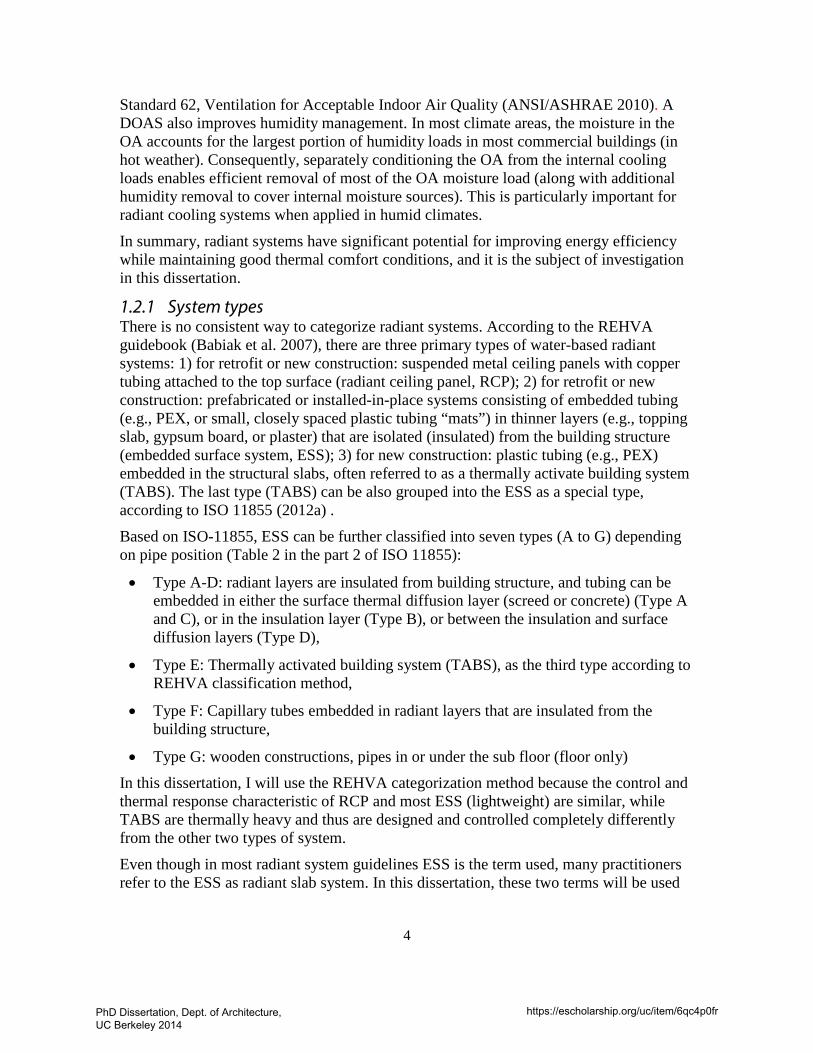
1.2.1 System types There is no consistent way to categorize radiant systems. According to the REHVA guidebook (Babiak et al. 2007), there are three primary types of water-based radiant systems: 1) for retrofit or new construction: suspended metal ceiling panels with copper tubing attached to the top surface (radiant ceiling panel, RCP); 2) for retrofit or new construction: prefabricated or installed-in-place systems consisting of embedded tubing (e.g., PEX, or small, closely spaced plastic tubing “mats”) in thinner layers (e.g., topping slab, gypsum board, or plaster) that are isolated (insulated) from the building structure (embedded surface system, ESS); 3) for new construction: plastic tubing (e.g., PEX) embedded in the structural slabs, often referred to as a thermally activate building system (TABS). The last type (TABS) can be also grouped into the ESS as a special type, according to ISO 11855 (2012a) .

Based on ISO-11855, ESS can be further classified into seven types (A to G) depending on pipe position (Table 2 in the part 2 of ISO 11855):

• Type A-D: radiant layers are insulated from building structure, and tubing can be embedded in either the surface thermal diffusion layer (screed or concrete) (Type A and C), or in the insulation layer (Type B), or between the insulation and surface diffusion layers (Type D),

• Type E: Thermally activated building system (TABS), as the third type according to REHVA classification method,

• Type F: Capillary tubes embedded in radiant layers that are insulated from the building structure,

• Type G: wooden constructions, pipes in or under the sub floor (floor only) In this dissertation, I will use the REHVA categorization method because the control and thermal response characteristic of RCP and most ESS (lightweight) are similar, while TABS are thermally heavy and thus are designed and controlled completely differently from the other two types of system.

Even though in most radiant system guidelines ESS is the term used, many practitioners refer to the ESS as radiant slab system. In this dissertation, these two terms will be used



5

interchangeably. Lightweight ESS is used to refer to the system types that are thermally decoupled from the building structures, and TABS is used to refer to heavyweight ESS.

Table 1-1: Schematic of the three types of radiant surface ceiling systems (based on the REHVA categorization method)

System types Schematics*

Radiant Cooling Panel

(RCP)

Embedded surface system

(ESS)

Thermally active building system (TABS)

*Graphs credit to Caroline Karmann, Center for the Built Environment



6

1.2.2 Applications in high performance buildings As they are increasingly seen as part of a comprehensive strategy for reducing energy usage, radiant systems have been specified and installed in many showcase high performance buildings (see Figure 1-1). Among those buildings, there are many located in climates that were traditionally considered as not favorable for radiant applications, including the National Renewable Energy Laboratories Research Support Facilities (Golden, Colo., 99% heating design temperature at -15.5 °C, and 1% cooling design dry bulb/wet bulb temperature at 32.0/15.1 °C) (Abellon 2011), Manitoba Hydro Place (Winnipeg, MB, Canada, 99% heating design temperature at -30.2 °C, and 1% cooling design dry bulb/wet bulb temperature at 28.9/ 19.9°C) (Kuwabara et al. 2011), and the Suvamabhumi Bangkok Airport (Bangkok, Thailand, 99% heating design temperature at 20 °C, and 1% cooling design dry bulb/wet bulb temperature at 36.6/ 26.4°C) (Simmonds et al. 2000). A database of representative buildings with radiant systems can be found at http://bit.ly/RadiantBuildingsCBE.

Figure 1-1: Examples of buildings with radiant systems installed1

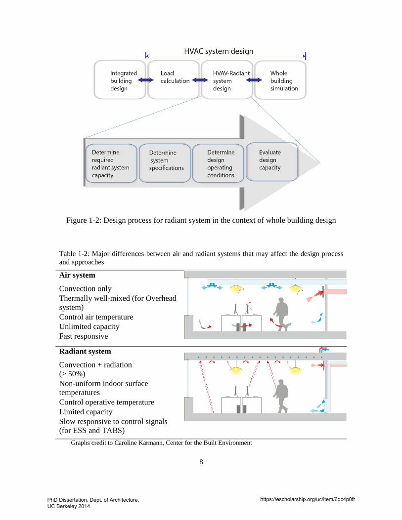
1.3 The Radiant system design process and its challenges The design process of a radiant system project is similar to the cases of air systems, including environmental load analysis, system design and sizing, and whole building evaluation for annual energy and thermal comfort performance. Figure 1-2 presents this general process in the context of whole building design.

1From top left: Suvamabhumi Bangkok Airport, 1998, Bangkok, Thailand (30% energy savings); NREL Research Support Facility, 2008, Golden, CO (LEED Platinum); Manitoba Hydro, 2009, Winnipeg, MB, Canada (LEED Platinum); David Brower Center, 2008, Berkeley, CA (LEED Platinum); Water + Life Museum, Hemet, CA (LEED Platinum); City Center-Crystals, Las Vegas, NV (LEED Gold).



http://bit.ly/RadiantBuildingsCBE

7

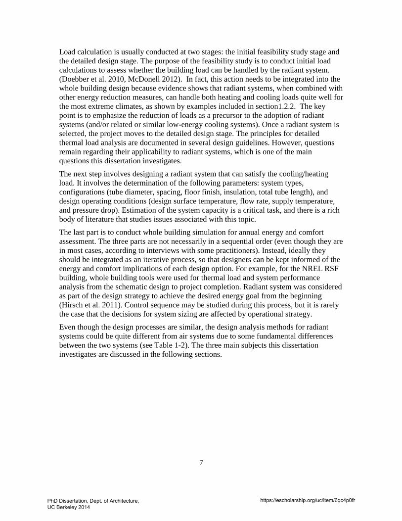
Load calculation is usually conducted at two stages: the initial feasibility study stage and the detailed design stage. The purpose of the feasibility study is to conduct initial load calculations to assess whether the building load can be handled by the radiant system. (Doebber et al. 2010, McDonell 2012). In fact, this action needs to be integrated into the whole building design because evidence shows that radiant systems, when combined with other energy reduction measures, can handle both heating and cooling loads quite well for the most extreme climates, as shown by examples included in section1.2.2. The key point is to emphasize the reduction of loads as a precursor to the adoption of radiant systems (and/or related or similar low-energy cooling systems). Once a radiant system is selected, the project moves to the detailed design stage. The principles for detailed thermal load analysis are documented in several design guidelines. However, questions remain regarding their applicability to radiant systems, which is one of the main questions this dissertation investigates.

The next step involves designing a radiant system that can satisfy the cooling/heating load. It involves the determination of the following parameters: system types, configurations (tube diameter, spacing, floor finish, insulation, total tube length), and design operating conditions (design surface temperature, flow rate, supply temperature, and pressure drop). Estimation of the system capacity is a critical task, and there is a rich body of literature that studies issues associated with this topic.

The last part is to conduct whole building simulation for annual energy and comfort assessment. The three parts are not necessarily in a sequential order (even though they are in most cases, according to interviews with some practitioners). Instead, ideally they should be integrated as an iterative process, so that designers can be kept informed of the energy and comfort implications of each design option. For example, for the NREL RSF building, whole building tools were used for thermal load and system performance analysis from the schematic design to project completion. Radiant system was considered as part of the design strategy to achieve the desired energy goal from the beginning (Hirsch et al. 2011). Control sequence may be studied during this process, but it is rarely the case that the decisions for system sizing are affected by operational strategy.

Even though the design processes are similar, the design analysis methods for radiant systems could be quite different from air systems due to some fundamental differences between the two systems (see Table 1-2). The three main subjects this dissertation investigates are discussed in the following sections.



8

Figure 1-2: Design process for radiant system in the context of whole building design

Table 1-2: Major differences between air and radiant systems that may affect the design process and approaches

Air system

Convection only Thermally well-mixed (for Overhead

system) Control air temperature Unlimited capacity Fast responsive

Radiant system

Convection + radiation (> 50%)

Non-uniform indoor surface temperatures

Control operative temperature Limited capacity Slow responsive to control signals

(for ESS and TABS)

Graphs credit to Caroline Karmann, Center for the Built Environment



9

1.3.1 Cooling load analysis method Air systems remove heat from a space by displacing warm air with cold air (convective heat transfer), while radiant systems provide cooling by direct radiation exchange with people and other heat sources in the space together by convective heat exchange with the zone air. The difference in the heat transfer mechanisms employed by the two systems may indicate a different definition of cooling load. In addition, compared to air systems, the presence of an actively cooled surface changes the heat transfer dynamics in a zone of a building. The chilled surface can instantaneously remove radiant heat (long and short wave) from any external (solar) or internal heat source, as well as interior surfaces (almost all will be warmer than the active surface), within its line-of-sight view. This means that radiant cooling systems may also affect zone cooling loads in several ways: (1) by cooling the inside surface temperatures of non-active exterior building walls, higher heat gain through the building envelope may result, thereby affecting total cooling energy, and (2) radiant heat exchange with non-active surfaces also reduces heat accumulation in the building mass, thereby affecting peak cooling loads.

Two research studies were identified that looked at heating load calculations in terms of the impact of the radiant system on wall surface temperatures and the resultant room load (Howell 1987, Chapman et al. 2000). However, both studies focused on heating load calculation under steady-state conditions. In another study, Chen (1990) suggested that the total heating load of a ceiling radiant heating system was 17% higher than that of the air heating system because of the role of thermal mass and higher heat loss through the building envelope due to slightly higher inside surface temperatures. For cooling applications, no studies were found on this topic, and in current radiant system design guidelines (CEN 2008, ASHRAE 2012a, ISO 2012), such impacts are not considered or evaluated.

Secondly, the interaction of building mass with heat source is influenced by the presence of activated radiant cooling surface(s). One phenomenon mentioned in the literature was radiant surface(s) as part of the building mass, instead of storing thermal energy as in the case of air systems, removes radiant heat gain (e.g. solar, radiative internal load and radiative envelope load) that is directly impinging on it. This phenomenon fundamentally changes the cooling load dynamics in a room. Niu (1997) pointed out that this direct radiation may create high peak cooling loads. He modified the thermal analysis program ACCURACY (Q. Chen and Kooi 1988) to account for the direct radiant heat gain as instantaneous cooling load for radiant systems. However, he did not describe how he implemented the modification, and the software is not accessible to the public. In an effort to understand the cooling load calculation process for radiant systems, Corgnati (Corgnati 2002) also tackled the direct radiant heat gain effect using a similar strategy to Niu’s. Based on Corgnati’s work, Causone et al. (2010) focused on the cases with the presence of direct solar gain. However, the methods proposed in these research studies only looked at the effect of direct radiant heat gain on cooling load, and the rest of the radiant heat gain and the convective heat gain are still considered to interact with the building mass as if the radiant system did not exist. In summary, no research can be found that fundamentally studies the differences of the heat transfer process in zones



10

conditioned by an air and a radiant system, and how these differences are going to impact the cooling load calculation and what could be the magnitude of the differences.

A fundamental understanding about how a radiant system interacts with the space differently from an air system can lead to answers to the following practical questions: Is the cooling load for a radiant system the same as for an air system? Can we use the same methods for load calculation? What are the implications for sizing and designing of radiant system? How might this affect the dynamic heat transfer modelling algorithm in a zone, and the selection of modelling tools for both load calculation and whole building performance evaluation?

1.3.2 Radiant system capacity estimation There are many models developed for predicting the performance of both the radiant panel and the embedded systems, and in section 2.4.2, I will give a comprehensive overview of those models. However, one challenging question that receives less research attention is the interaction between the radiant system surfaces with its thermal surroundings. When a radiant system is exposed to a dynamic environment with constantly changing loads, the questions are to what extend could the environmental conditions and the various heat sources in the space affect radiant system performance? Is it important to consider the impacts at all? How to consider them if the impacts are significant?

Research has shown that radiant system cooling capacity could be enhanced by 30% with the presence of an air diffuser (Jeong and Mumma 2003). This is because, in current cooling capacity estimation methods, forced convective heat transfer between room air and radiant surfaces induced by air diffusers installed at the ceiling level were not considered.

Another example is that cooling capacity could be enhanced up 17% if surface temperatures of non-radiant surfaces, such as exterior wall or glazing, are higher than the air temperature (Tian et al. 2012). This result can lead to questions regarding the accuracy of radiant panel manufacturers’ system performance data when apply to the design for spaces that are under non-standardized thermal conditions. Currently, the performance data are obtained under standardized conditions, including predefined differential temperature between water loop and room reference temperature, types of heat gain (representing people), and room conditions (for example, less than 1°K difference between air and wall surface temperatures per EN 14240). Indeed, methods to define a standardized testing condition remain inconsistent so far. While the test chamber prescribed in EN 14240 represents an interior zone, featuring uniform air and wall surface temperature and internal load representing a person, the testing chamber prescribed by ASHRAE 138 represents a perimeter zone without window, featured by one wall with higher wall surface temperature, and the heat gain is conductive heat instead of internal load. Therefore, it could be quite possible that manufacturers can generate different performance data for the same products depending on which testing standard they adopted. For rating purpose, different radiant panels should be tested under the same conditions that tend to produce a conservative output, but the question becomes, for the purpose of optimizing the design, whether the manufacturers need to provide



11

performance data for different environmental conditions, so that designers can be better informed during design.

The third example regards the design when the sun illuminates the radiant cooling surfaces. The guideline for standard application of a radiant floor cooling system is a maximum cooling capacity of 42 W/m2 (Olesen 1997, Olesen et al. 2000). However, for the cases with direct solar radiation, the cooling capacity can increase significantly, reaching 80–100 W/m2 (Zhao et al. 2013, Borresen 1994, Odyjas and Gorka 2013). For this reason, floor cooling is increasingly designed for those spaces with large glazed surfaces, such as atriums, airports, and entrance halls (Simmonds et al. 2000, Nall 2013). However, there is still no practical method for designers to use when designing for these cases, which is one of the topics investigated in this dissertation.

To improve the current design methods, it is important to understand, theoretically, why there are limitations, and what the implications are for sizing and designing the radiant systems and their associated air systems when the standardized methods do not apply.

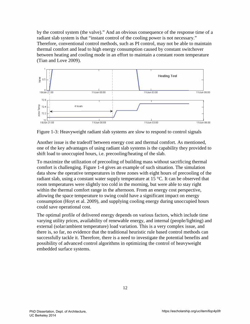
1.3.3 Control considerations Design methods for radiant systems can be quite different depending on the type of radiant system, and in particularly the system’s control characteristics. Radiant panel systems and lightweight embedded systems are fast responsive to control signals and are able to change space conditions relatively fast, and thus sizing of those systems based on a peak cooling load could be adequate. Control strategy is deliberately simplified and is not considered for design analysis. However, for heavyweight embedded surface systems, mostly TABS, that are designed and controlled for load shifting, sizing based on a peak load is unlikely to be a good solution. Load shifting consists of shaping the energy profile delivered to a building, exploiting the possibility of storing energy for later use. As Lehman et al. (2007) pointed out, due to the large thermal inertia associated with the mass in the radiant slabs, thermal conditions on the room side are almost unaffected from the processes on the hydronic side. In the cooling case, this allows for the pre-cooling period of the fabric being extended to 24 hour a day with accordingly ‘‘high’’ supply temperatures and peak load reductions of up to 50%. Thus, the sizing strategy of the radiant slabs and the associated equipment at the plant side (chiller, pump, etc.) should take into account more than just room side cooling load, but also a control strategy.

Compared to air systems, there are many challenges in the control of heavyweight ESS. First, with water pipes embedded in radiant layers, the systems are slow to respond to control signals due to large thermal inertia. The response time depends on the depth of the tube and the heat capacity of the radiant slab, and usually the time constant can be up to couple hours (Babiak et al. 2007). Figure 1-3 shows monitored room temperature during a pulse-heating test in the David Brower Center, a building equipped with a radiant slab ceiling system in Berkeley, CA. The top plot shows that the heating valve was turned on at 9 p.m. and turned off at around 2 a.m. (the hot water temperature was at 32 °C). And the bottom plot shows that the room air temperature remained unaffected until four hours after the heating valve turned on. As suggested in the REHVA Guidebook (Babiak et al. 2007), “thermal gain/loss leading to increased/decreased cooling load with characteristic times shorter than time constant cannot be compensated



12

by the control system (the valve).” And an obvious consequence of the response time of a radiant slab system is that “instant control of the cooling power is not necessary.” Therefore, conventional control methods, such as PI control, may not be able to maintain thermal comfort and lead to high energy consumption caused by constant switchover between heating and cooling mode in an effort to maintain a constant room temperature (Tian and Love 2009).

Figure 1-3: Heavyweight radiant slab systems are slow to respond to control signals

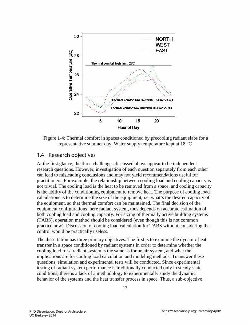
Another issue is the tradeoff between energy cost and thermal comfort. As mentioned, one of the key advantages of using radiant slab systems is the capability they provided to shift load to unoccupied hours, i.e. precooling/heating of the slab.

To maximize the utilization of precooling of building mass without sacrificing thermal comfort is challenging. Figure 1-4 gives an example of such situation. The simulation data show the operative temperatures in three zones with eight hours of precooling of the radiant slab, using a constant water supply temperature at 15 °C. It can be observed that room temperatures were slightly too cold in the morning, but were able to stay right within the thermal comfort range in the afternoon. From an energy cost perspective, allowing the space temperature to swing could have a significant impact on energy consumption (Hoyt et al. 2009), and supplying cooling energy during unoccupied hours could save operational cost.

The optimal profile of delivered energy depends on various factors, which include time varying utility prices, availability of renewable energy, and internal (people/lighting) and external (solar/ambient temperature) load variation. This is a very complex issue, and there is, so far, no evidence that the traditional heuristic rule based control methods can successfully tackle it. Therefore, there is a need to investigate the potential benefits and possibility of advanced control algorithms in optimizing the control of heavyweight embedded surface systems.



13

Figure 1-4: Thermal comfort in spaces conditioned by precooling radiant slabs for a

representative summer day: Water supply temperature kept at 18 °C

1.4 Research objectives At the first glance, the three challenges discussed above appear to be independent research questions. However, investigation of each question separately from each other can lead to misleading conclusions and may not yield recommendations useful for practitioners. For example, the relationship between cooling load and cooling capacity is not trivial. The cooling load is the heat to be removed from a space, and cooling capacity is the ability of the conditioning equipment to remove heat. The purpose of cooling load calculations is to determine the size of the equipment, i.e. what’s the desired capacity of the equipment, so that thermal comfort can be maintained. The final decision of the equipment configurations, here radiant system, thus depends on accurate estimation of both cooling load and cooling capacity. For sizing of thermally active building systems (TABS), operation method should be considered (even though this is not common practice now). Discussion of cooling load calculation for TABS without considering the control would be practically useless.

The dissertation has three primary objectives. The first is to examine the dynamic heat transfer in a space conditioned by radiant systems in order to determine whether the cooling load for a radiant system is the same as for an air system, and what the implications are for cooling load calculation and modeling methods. To answer these questions, simulation and experimental tests will be conducted. Since experimental testing of radiant system performance is traditionally conducted only in steady-state conditions, there is a lack of a methodology to experimentally study the dynamic behavior of the systems and the heat transfer process in space. Thus, a sub-objective



14

associated with the study is to develop a dynamic method of testing radiant system cooling load, and comparing the dynamic behavior of radiant and air systems when exposed to a typical internal load. More broadly, the answer to this question can be applied to all space conditioning systems that involve radiation heat transfer, such as underfloor air distribution systems (UFAD), and displacement ventilation, which will create non-uniform surface temperatures in the space.

The second objective is to identify the limitations in the applicability of current cooling capacity estimation methods, to quantitatively evaluate the cooling capacity of radiant systems when exposed to shortwave heat sources with a focus on direct solar load, and to develop a new simplified method for design of those cases.

The last objective is to investigate the control methods for heavyweight radiant slab systems, in particularly the energy and comfort benefits of a model-based predictive control method. In order to simplify the controller for easy implementation, a secondary objective of this study is to create a simplified dynamic model of a radiant slab system for implementation in model predictive controllers.

1.5 Organization of the dissertation Chapter 2 starts with an introduction of the fundamental heat transfer theory related to the design and operation of radiant systems. It then provides a review of the standard methods for thermal load analysis and radiant system modeling/design and the development of control methods for the heavyweight radiant systems. This helps to develop a framework for understanding the attributes of each method, and assumptions commonly used in the research world. This is followed up with a descriptive analysis of interviews/surveys of practitioners and manufacturers, and case studies. The main questions asked focused on understanding what is the design process in practice, which tools and why are they used for different design analyses, and whether there are gaps between standard design methods and their applications. At the end of Chapter 2, I further discuss the issues associated with the current design methods, and propose research questions.

Chapters 3–5 examine dynamic heat transfer in spaces conditioned by radiant systems, and the implications for cooling load calculation and modeling methods. Chapter 3 focuses on theoretical analysis and uses an energy simulation tool based on first principles to examine the differences between radiant and air systems. Chapter 4 presents an experimental study that was designed to capture the transient behavior of space conditioned by both radiant and air systems, and the results of the experiment are used to verify the simulation results in Chapter 3 and for further analysis for Chapter 5. Based on the previous two chapters, Chapter 5 develops recommendations for the radiant systems for: 1) cooling load calculation procedure and method selection, 2) cooling load definitions for different radiant system types, 3) modeling methods and tool selection, and 4) improvements in design guidelines.

Chapter 6 theoretically and numerically analyzes the impacts of solar heat gain on radiant floor cooling capacity, and proposes an improved practical approach for estimating the system cooling capacity and the sizing of the associated air system.



15

Chapter 7 presents a case study of the control of a radiant system in an office building in Berkeley, and compares the performance of different control strategies for extended climatic conditions using energy simulation of a calibrated building energy model.

Chapter 8 presents the implications of the key findings and suggests directions for future work.



16

2 BACKGROUND

This chapter starts with an introduction of the fundamental heat transfer theory related to the design and operation of radiant systems. Then I review the methods documented in the literature for thermal load analysis and radiant system capacity estimation, together with the research efforts in developing control methods for heavyweight radiant systems. At the end of each section, there are discussions about the issues associated with current methods and research needs. Aiming to understand the state of the art in the industry, the last section of the chapter provides a descriptive analysis of methods used by leading practitioners and manufactures collected from interviews, surveys, and case studies reports.

2.1 The heat transfer theory The fundamental heat transfer processes involved in building thermal analysis are well documented, and can be found in handbooks and many textbooks (Kuehn et al. 1998, ASHRAE 2009, DOE 2011, Howell et al. 2011). In this section I review the related knowledge that can help understand how radiant systems interact with the thermal environment.

Compared to the air-based conditioning system, a radiant system is unique because it is a case when the HVAC system becomes part of the building elements, and the interactions of the radiant system with the ever changing space thermal conditions become particularly crucial for design analysis and control purposes (Stetiu et al. 1995, Weitzmann 2004, Strand and Baumgartner 2005, Olesen et al. 2006). Understanding these dynamics is fundamental for the development of design calculations and control methods. Overall, there are two heat transfer process involved: the heat transfer between the radiant layer surface and the space it is conditioning and the processes between the radiant layer and the water loop.

2.1.1 Heat transfer at radiant cooling surfaces Radiant systems remove the sensible heat in a room at the radiant surfaces. Figure 2-1 shows the heat transfer balance at the surface. If one defines the control volume as the inside face of the cooling slab, with a positive sign meaning heat is being transferred into the control volume and negative indicates heat leaving the control volume, the heat balance equation can be written as follows:

𝑞𝑞𝑐𝑜𝑛𝑣" + 𝑞𝑞𝑙𝑤,𝑠𝑢𝑟𝑓" + q𝑙𝑤,𝑖𝑛𝑡

" + 𝑞𝑞𝑠𝑤,𝑠𝑜𝑙" + 𝑞𝑞𝑠𝑤,𝑖𝑛𝑡

" + 𝑞𝑞𝑐𝑜𝑛𝑑" = 0 Equation 2-1

In which,

𝑞𝑞"𝑐𝑜𝑛𝑣 = Convection heat transfer at the exposed face of the cooling surface(s), W/m2

𝑞𝑞𝑙𝑤,𝑠𝑢𝑟𝑓" = Net longwave radiation flux to radiant active surface from other surfaces,

W/m2;

𝑞𝑞𝑙𝑤,𝑖𝑛𝑡" = longwave radiant exchange flux from the internal load, W/m2



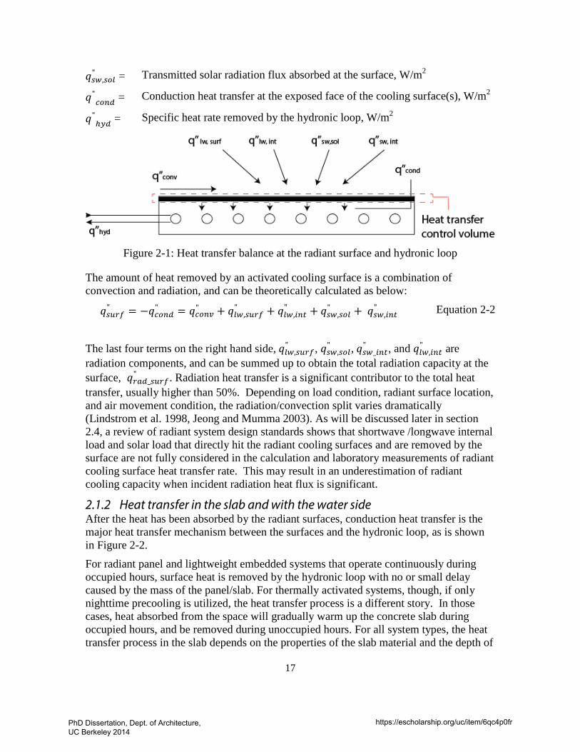
17

𝑞𝑞𝑠𝑤,𝑠𝑜𝑙" = Transmitted solar radiation flux absorbed at the surface, W/m2

𝑞𝑞"𝑐𝑜𝑛𝑑 = Conduction heat transfer at the exposed face of the cooling surface(s), W/m2

𝑞𝑞"ℎ𝑦𝑑 = Specific heat rate removed by the hydronic loop, W/m2

Figure 2-1: Heat transfer balance at the radiant surface and hydronic loop

The amount of heat removed by an activated cooling surface is a combination of convection and radiation, and can be theoretically calculated as below:

𝑞𝑞𝑠𝑢𝑟𝑓" = −𝑞𝑞𝑐𝑜𝑛𝑑" = 𝑞𝑞𝑐𝑜𝑛𝑣" + 𝑞𝑞𝑙𝑤,𝑠𝑢𝑟𝑓" + 𝑞𝑞𝑙𝑤,𝑖𝑛𝑡

" + 𝑞𝑞𝑠𝑤,𝑠𝑜𝑙" + 𝑞𝑞𝑠𝑤,𝑖𝑛𝑡

" Equation 2-2

The last four terms on the right hand side, 𝑞𝑞𝑙𝑤,𝑠𝑢𝑟𝑓" , 𝑞𝑞𝑠𝑤,𝑠𝑜𝑙

" , 𝑞𝑞𝑠𝑤_𝑖𝑛𝑡" , and 𝑞𝑞𝑙𝑤,𝑖𝑛𝑡

" are radiation components, and can be summed up to obtain the total radiation capacity at the surface, 𝑞𝑞𝑟𝑎𝑑_𝑠𝑢𝑟𝑓

" . Radiation heat transfer is a significant contributor to the total heat transfer, usually higher than 50%. Depending on load condition, radiant surface location, and air movement condition, the radiation/convection split varies dramatically (Lindstrom et al. 1998, Jeong and Mumma 2003). As will be discussed later in section 2.4, a review of radiant system design standards shows that shortwave /longwave internal load and solar load that directly hit the radiant cooling surfaces and are removed by the surface are not fully considered in the calculation and laboratory measurements of radiant cooling surface heat transfer rate. This may result in an underestimation of radiant cooling capacity when incident radiation heat flux is significant.

2.1.2 Heat transfer in the slab and with the water side After the heat has been absorbed by the radiant surfaces, conduction heat transfer is the major heat transfer mechanism between the surfaces and the hydronic loop, as is shown in Figure 2-2.

For radiant panel and lightweight embedded systems that operate continuously during occupied hours, surface heat is removed by the hydronic loop with no or small delay caused by the mass of the panel/slab. For thermally activated systems, though, if only nighttime precooling is utilized, the heat transfer process is a different story. In those cases, heat absorbed from the space will gradually warm up the concrete slab during occupied hours, and be removed during unoccupied hours. For all system types, the heat transfer process in the slab depends on the properties of the slab material and the depth of



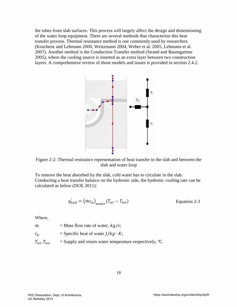
18

the tubes from slab surfaces. This process will largely affect the design and dimensioning of the water loop equipment. There are several methods that characterize this heat transfer process. Thermal resistance method is one commonly used by researchers (Koschenz and Lehmann 2000, Weitzmann 2004, Weber et al. 2005, Lehmann et al. 2007). Another method is the Conduction Transfer method (Strand and Baumgartner 2005), where the cooling source is inserted as an extra layer between two construction layers. A comprehensive review of those models and issues is provided in section 2.4.2.

Figure 2-2: Thermal resistance representation of heat transfer in the slab and between the

slab and water loop

To remove the heat absorbed by the slab, cold water has to circulate in the slab. Conducting a heat transfer balance on the hydronic side, the hydronic cooling rate can be calculated as below (DOE 2011):

𝑞𝑞ℎ𝑦𝑑" = ��𝑐𝑝�𝑤𝑎𝑡𝑒𝑟(𝑇𝑤𝑖 − 𝑇𝑤𝑜) Equation 2-3

Where,

�� = Mass flow rate of water, 𝑘𝑔/𝑠𝑠;

𝑐𝑝 = Specific heat of water 𝐽/𝑘𝑔 ∙ 𝐾;

𝑇𝑤𝑖,𝑇𝑤𝑜 = Supply and return water temperature respectively, ℃.



19

2.2 Design guidelines There are many design guidelines related to the design process of radiant systems ( Table 2-1). Some of them provide analysis methods that are generally applicable to all types of HVAC systems, and some of them are dedicated for a specific type of radiant system. They play critical roles by providing guidance to practitioners for load analysis, system performance testing, and modeling. This part offers an overview of their roles and coverage. In the later parts, I will review the documented methods for the topics of interest of the dissertation.

EN 14240 (CEN 2004) and EN 14037 (CEN 2013) provide standardized testing methods for evaluating radiant panel systems (RCP) thermal performance. EN 14240 covers cooling applications and EN 14037 covers heating. A new version of EN 14037 is currently under development, which is supposed to cover both heating and cooling applications.

EN 1264 (CEN 2011), EN 15377 (CEN 2008), and ISO 11855 (2012c) are standards for embedded surface systems. EN 1264 was originally developed for designing embedded radiant floor heating systems. And it provides methods for the determination of the thermal output of floor heating systems using calculation and test methods. A new part, Part 5, was recently included for other surfaces (ceiling, walls) and also for cooling. The standard EN 15377 includes calculation methods for design and dimensioning of embedded radiant heating and cooling systems. For some system types (Type A/B/C/D) the same calculation methods as in EN 1264 are used. For other system types (Type E, F, G) that are not covered by EN 1264, new calculation methods are introduced. Included also in the standard is a dedicated part (Part 3) that deals with systems Type E (TABS), a system with pipes embedded directly in the building structure mass. The content of ISO 11855 is consistent with what is covered in EN 1264 and EN 15377. Even though most radiant slab manufacturers refer to EN 15377 or EN 1264 when reporting performance data, I refer to ISO 11855 throughout this dissertation because its coverage is the most comprehensive, including also hydronic side sizing strategies, control, etc. Another guidebook worth mentioning is the REHVA guidebook on low temperature heating and high temperature cooling. It references the standards mentioned here for design calculation methods, but uses more descriptive language and discusses some issues that designers might encounter in practice.

All the standards mentioned above focus on the design of the radiant system itself and its hydronic system; thermal load analysis is not a topic covered. They reference other standards, such as EN 15243 (CEN 2007a) or EN 15255 (CEN 2007c), for load calculation. These two standards, as indicated by their titles, provide general guidance for load analysis procedures in HVAC systems design. They do not provide a detailed calculation method.

In the United States, chapter 6 of ASHRAE HVAC system and equipment (ASHRAE 2012a) provides radiant system design principles and steady-state sizing algorithms. Chapter 18 and 19 of ASHRAE Handbook of Fundamentals present thermal load analysis and modeling methods, respectively. ASHRAE 138 is the US counterpart of EN 14240.



20

Besides the design standards developed by official organizations, manuals developed by radiant system design firms, manufacturers, and independent consultants also have wide influence on the practice. For example, Uponor, a major radiant slab manufacture, has developed comprehensive radiant system design manuals, which are widely referred to as a source of design information. Its manual published in 2011 focuses on residential heating applications (Uponor 2011), and the 2013 radiant cooling design manual discusses unique features and challenges for cooling applications (Uponor 2013). Price Industries, a major radiant panel manufacturer, has also published a series of design handbooks, and the Engineer’s HVAC Handbook Chapter 18 titled “Introduction to radiant heating and cooling” is reviewed.



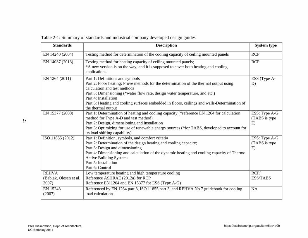
Table 2-1: Summary of standards and industrial company developed design guides

21

Standards Description System type

EN 14240 (2004) Testing method for determination of the cooling capacity of ceiling mounted panels RCP

EN 14037 (2013) Testing method for heating capacity of ceiling mounted panels; *A new version is on the way, and it is supposed to cover both heating and cooling applications.

RCP

EN 1264 (2011) Part 1: Definitions and symbols Part 2: Floor heating: Prove methods for the determination of the thermal output using calculation and test methods Part 3: Dimensioning (*water flow rate, design water temperature, and etc.) Part 4: Installation Part 5: Heating and cooling surfaces embedded in floors, ceilings and walls-Determination of the thermal output

ESS (Type A-D)

EN 15377 (2008) Part 1: Determination of heating and cooling capacity (*reference EN 1264 for calculation method for Type A-D and test method) Part 2: Design, dimensioning and installation Part 3: Optimizing for use of renewable energy sources (*for TABS, developed to account for its load shifting capability)

ESS: Type A-G (TABS is type E)

ISO 11855 (2012) Part 1: Definition, symbols, and comfort criteria Part 2: Determination of the design heating and cooling capacity; Part 3: Design and dimensioning Part 4: Dimensioning and calculation of the dynamic heating and cooling capacity of Thermo Active Building Systems Part 5: Installation Part 6: Control

ESS: Type A-G (TABS is type E)

REHVA (Babiak, Olesen et al. 2007)

Low temperature heating and high temperature cooling Reference ASHRAE (2012a) for RCP Reference EN 1264 and EN 15377 for ESS (Type A-G)

RCP/ ESS/TABS

EN 15243 (2007)

Referenced by EN 1264 part 3, ISO 11855 part 3, and REHVA No.7 guidebook for cooling load calculation

NA



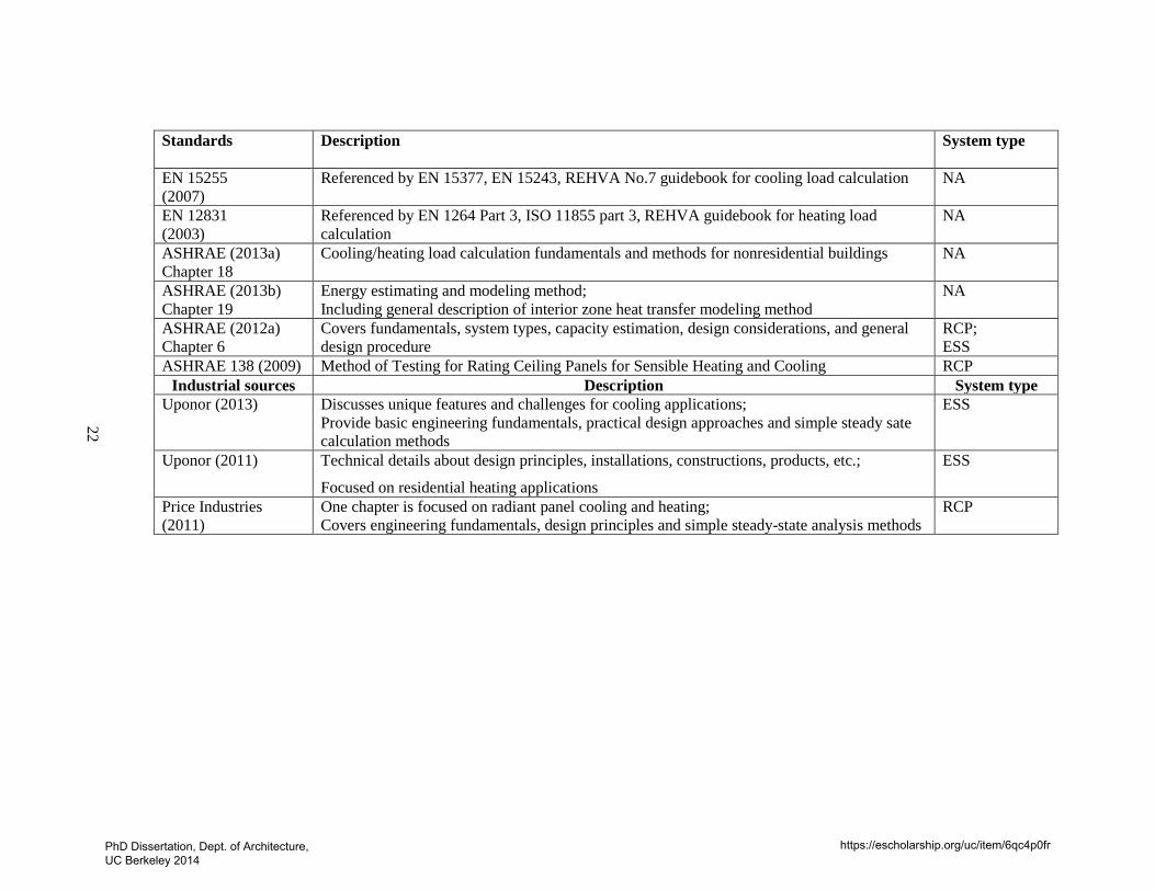
22

Standards

Description System type

EN 15255 (2007)

Referenced by EN 15377, EN 15243, REHVA No.7 guidebook for cooling load calculation NA

EN 12831 (2003)

Referenced by EN 1264 Part 3, ISO 11855 part 3, REHVA guidebook for heating load calculation

NA

ASHRAE (2013a) Chapter 18

Cooling/heating load calculation fundamentals and methods for nonresidential buildings NA

ASHRAE (2013b) Chapter 19

Energy estimating and modeling method; Including general description of interior zone heat transfer modeling method

NA

ASHRAE (2012a) Chapter 6

Covers fundamentals, system types, capacity estimation, design considerations, and general design procedure

RCP; ESS

ASHRAE 138 (2009) Method of Testing for Rating Ceiling Panels for Sensible Heating and Cooling RCP Industrial sources Description System type

Uponor (2013) Discusses unique features and challenges for cooling applications; Provide basic engineering fundamentals, practical design approaches and simple steady sate calculation methods

ESS

Uponor (2011) Technical details about design principles, installations, constructions, products, etc.;

Focused on residential heating applications

ESS

Price Industries (2011)

One chapter is focused on radiant panel cooling and heating; Covers engineering fundamentals, design principles and simple steady-state analysis methods

RCP



23

2.3 Cooling load analysis methods I focus on cooling applications, since the heating load calculation process is relatively simple for two reasons: 1) to simulate the worst case scenario any type of heat source (internal or solar heat gain) is not considered, and 2) steady-state calculation is considered adequate for the same reason.

The purpose of conducting a cooling load analysis is to support the sizing of HVAC equipment. In the case of radiant systems, it is used to determine the required cooling output of the radiating surface. How to define a design cooling load is the first issue, and another issue is the calculation algorithm. Table 2-2 provides a summary of load analysis methods, including definitions, features of the algorithm (steady-state or dynamic), sizing strategies, and applicable system types. Note that only original sources are listed, and the last column of the table provides cross-reference information.

2.3.1 Cooling load definitions In the ASHRAE Handbook (ASHRAE 2013a), a design sensible cooling load is the peak value of the design day-cooling load, which is defined as “the rate at which sensible heat must be removed from the zone air to maintain a constant air temperature”. Cooling load is also independent of HVAC system types and operating strategies. This implies that the cooling load for a radiant system is assumed to be the same as for an air system. Three features of the definition are: 1) a cooling load is obtained to balance the heat transfer of the air volume in space; 2) the air temperature is the reference temperature; 3) the temperature setpoint is a constant value.

As mentioned, EN 1264, EN 15377, and ISO 11855 reference EN15243 and EN 15255 for load analysis for most types of embedded systems. However, for thermally active building systems (type E), both EN 15377 and ISO 11855 have parts dedicated to discussing design and sizing methods. Four sizing methods are provided, including a rough sizing method, a simplified sizing by diagram method, a method based on finite difference method, and a method that uses a dynamic building simulation program. In the rough sizing method, the cooling load is defined as heat to be removed by the radiant system at the surface level, and can be calculated as the daily energy gain (internal heat plus solar gain) divided by the radiant system operation hours, i.e. the average total heat gain. Three features of this definition are: 1) the cooling load is obtained by heat balance at the radiant surface; 2) an average of daily total heat gain is used as the cooling load instead of a peak value; 3) the system is sized to allow the space operative temperature to float within a thermal comfort range instead of maintaining a constant value. The three features are also reflected in the simplified sizing by diagram method. Sizing of the system based on an average of total heat gain instead of a peak value can be supported by the fact that time constants for thermally massive systems are large so it is not feasible to control the hydronic system in response to short-term environmental changes to meet a peak design load (load, setpoint changes) (Babiak 2007, Olesen 2007a, Lehmann et al. 2007).

In summary, there are inconsistences between standards in defining cooling load, and the major question is does the definition of cooling load depend on the HVAC system or not?



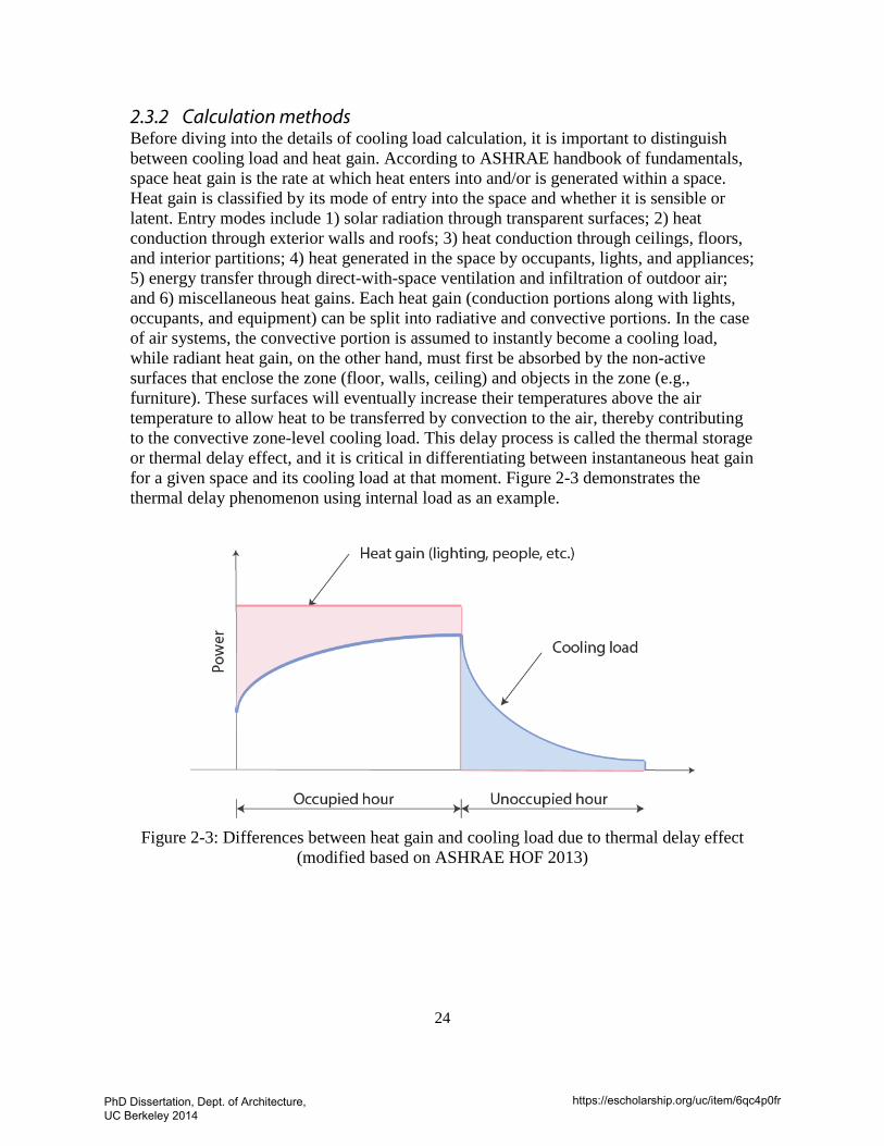
24

2.3.2 Calculation methods Before diving into the details of cooling load calculation, it is important to distinguish between cooling load and heat gain. According to ASHRAE handbook of fundamentals, space heat gain is the rate at which heat enters into and/or is generated within a space. Heat gain is classified by its mode of entry into the space and whether it is sensible or latent. Entry modes include 1) solar radiation through transparent surfaces; 2) heat conduction through exterior walls and roofs; 3) heat conduction through ceilings, floors, and interior partitions; 4) heat generated in the space by occupants, lights, and appliances; 5) energy transfer through direct-with-space ventilation and infiltration of outdoor air; and 6) miscellaneous heat gains. Each heat gain (conduction portions along with lights, occupants, and equipment) can be split into radiative and convective portions. In the case of air systems, the convective portion is assumed to instantly become a cooling load, while radiant heat gain, on the other hand, must first be absorbed by the non-active surfaces that enclose the zone (floor, walls, ceiling) and objects in the zone (e.g., furniture). These surfaces will eventually increase their temperatures above the air temperature to allow heat to be transferred by convection to the air, thereby contributing to the convective zone-level cooling load. This delay process is called the thermal storage or thermal delay effect, and it is critical in differentiating between instantaneous heat gain for a given space and its cooling load at that moment. Figure 2-3 demonstrates the thermal delay phenomenon using internal load as an example.

Figure 2-3: Differences between heat gain and cooling load due to thermal delay effect

(modified based on ASHRAE HOF 2013)



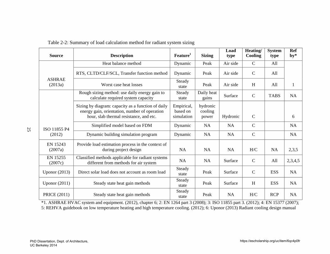
Table 2-2: Summary of load calculation method for radiant system sizing

25

Source Description Feature1 Sizing Load type

Heating/ Cooling

System type

Ref by*

ASHRAE (2013a)

Heat balance method Dynamic Peak Air side C All

1

RTS, CLTD/CLF/SCL, Transfer function method Dynamic Peak Air side C All

Worst case heat losses Steady state Peak Air side H All

ISO 11855 P4 (2012)

Rough sizing method: use daily energy gain to calculate required system capacity

Steady state

Daily heat gains Surface C TABS NA

Sizing by diagram: capacity as a function of daily energy gain, orientation, number of operation

hour, slab thermal resistance, and etc.

Empirical, based on

simulation

hydronic cooling power Hydronic C 6

Simplified model based on FDM Dynamic NA NA C NA

Dynamic building simulation program Dynamic NA NA C NA

EN 15243 (2007a)

Provide load estimation process in the context of during project design NA NA NA H/C NA 2,3,5

EN 15255 (2007c)

Classified methods applicable for radiant systems different from methods for air system

NA NA Surface C All 2,3,4,5

Uponor (2013) Direct solar load does not account as room load Steady state Peak Surface C ESS NA

Uponor (2011) Steady state heat gain methods Steady state Peak Surface H ESS NA

PRICE (2011) Steady state heat gain methods Steady state Peak NA H/C RCP NA

*1. ASHRAE HVAC system and equipment. (2012), chapter 6; 2: EN 1264 part 3 (2008); 3: ISO 11855 part 3. (2012); 4: EN 15377 (2007); 5: REHVA guidebook on low temperature heating and high temperature cooling. (2012); 6: Uponor (2013) Radiant cooling design manual



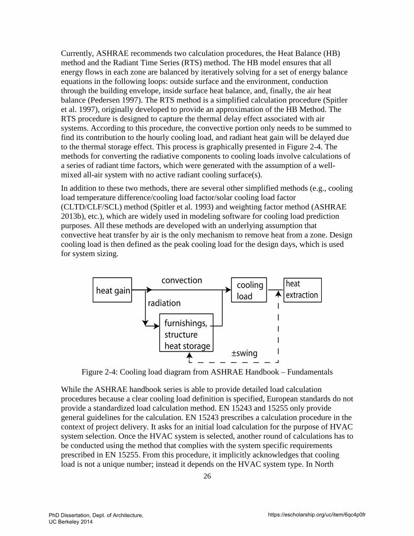
26

Currently, ASHRAE recommends two calculation procedures, the Heat Balance (HB) method and the Radiant Time Series (RTS) method. The HB model ensures that all energy flows in each zone are balanced by iteratively solving for a set of energy balance equations in the following loops: outside surface and the environment, conduction through the building envelope, inside surface heat balance, and, finally, the air heat balance (Pedersen 1997). The RTS method is a simplified calculation procedure (Spitler et al. 1997), originally developed to provide an approximation of the HB Method. The RTS procedure is designed to capture the thermal delay effect associated with air systems. According to this procedure, the convective portion only needs to be summed to find its contribution to the hourly cooling load, and radiant heat gain will be delayed due to the thermal storage effect. This process is graphically presented in Figure 2-4. The methods for converting the radiative components to cooling loads involve calculations of a series of radiant time factors, which were generated with the assumption of a well-mixed all-air system with no active radiant cooling surface(s).

In addition to these two methods, there are several other simplified methods (e.g., cooling load temperature difference/cooling load factor/solar cooling load factor (CLTD/CLF/SCL) method (Spitler et al. 1993) and weighting factor method (ASHRAE 2013b), etc.), which are widely used in modeling software for cooling load prediction purposes. All these methods are developed with an underlying assumption that convective heat transfer by air is the only mechanism to remove heat from a zone. Design cooling load is then defined as the peak cooling load for the design days, which is used for system sizing.

Figure 2-4: Cooling load diagram from ASHRAE Handbook – Fundamentals

While the ASHRAE handbook series is able to provide detailed load calculation procedures because a clear cooling load definition is specified, European standards do not provide a standardized load calculation method. EN 15243 and 15255 only provide general guidelines for the calculation. EN 15243 prescribes a calculation procedure in the context of project delivery. It asks for an initial load calculation for the purpose of HVAC system selection. Once the HVAC system is selected, another round of calculations has to be conducted using the method that complies with the system specific requirements prescribed in EN 15255. From this procedure, it implicitly acknowledges that cooling load is not a unique number; instead it depends on the HVAC system type. In North



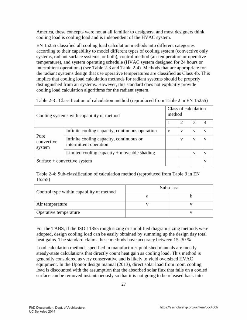
27

America, these concepts were not at all familiar to designers, and most designers think cooling load is cooling load and is independent of the HVAC system.

EN 15255 classified all cooling load calculation methods into different categories according to their capability to model different types of cooling system (convective only systems, radiant surface systems, or both), control method (air temperature or operative temperature), and system operating schedule (HVAC system designed for 24 hours or intermittent operations) (see Table 2-3 and Table 2-4). Methods that are appropriate for the radiant systems design that use operative temperatures are classified as Class 4b. This implies that cooling load calculation methods for radiant systems should be properly distinguished from air systems. However, this standard does not explicitly provide cooling load calculation algorithms for the radiant system.

Table 2-3 : Classification of calculation method (reproduced from Table 2 in EN 15255)

Cooling systems with capability of method Class of calculation method

1 2 3 4

Pure convective system

Infinite cooling capacity, continuous operation v v v v

Infinite cooling capacity, continuous or intermittent operation

v v v

Limited cooling capacity + moveable shading v v

Surface + convective system v

Table 2-4: Sub-classification of calculation method (reproduced from Table 3 in EN 15255)

Control type within capability of method Sub-class

a b

Air temperature v v

Operative temperature v

For the TABS, if the ISO 11855 rough sizing or simplified diagram sizing methods were adopted, design cooling load can be easily obtained by summing up the design day total heat gains. The standard claims these methods have accuracy between 15–30 %.

Load calculation methods specified in manufacturer-published manuals are mostly steady-state calculations that directly count heat gain as cooling load. This method is generally considered as very conservative and is likely to yield oversized HVAC equipment. In the Uponor design manual (2013), direct solar load from room cooling load is discounted with the assumption that the absorbed solar flux that falls on a cooled surface can be removed instantaneously so that it is not going to be released back into



28

space and become room cooling load. This concept, when presented, tends to be misleading because it makes people think that the cooling load for a radiant system is smaller because solar load does not need to be considered as part of room cooling load. However, it is still heat that needs to be removed, and the HVAC equipment has to be sized to be able to remove that heat.

2.3.3 Summary In summary, ASHRAE standards give a universal cooling load definition and provide detailed load calculation methods that apply to any HVAC system, while European or ISO standards, without suggesting detailed calculation algorithms, imply that the definition and methods may depend on system types, operating hours, and temperature control strategy. So the questions regarding the definition of cooling load and the calculation algorithm are:

• Is it correct to assume cooling load definition can be independent of system type?

• Is it correct that the same calculation method can be used for the load calculation for radiant systems as for air systems?

• Should operating strategies or temperature control methods (operative /air temperature) be considered in the load calculation process?

The answer to the second question may be controversial as it is related to design concept, and the first question is related to the fundamental heat transfer differences in the space when conditioned by different HVAC systems. Unlike the case of air systems where the cooling load is purely convective, the cooling load for radiant systems consists of both convective and radiant components, thus there is no fundamental reason to expect the cooling loads for the two systems to be the same. In this dissertation, I will investigate these questions and provide the answers.

2.4 Radiant system capacity evaluation methods The goal for designing a radiant system is to assure that the system has a capacity that can match a desired cooling/heating load, which can be the total or part of the total load. Design principles and procedures of radiant systems can be found in many publications (Olesen 1997b, Babiak 2007, Uponor 2011, ASHRAE 2012a). The process generally involves the determination of the following parameters: system types, specifications (tube diameter, spacing, floor finish, insulation, total tube length), and design operating conditions (surface temperature, flow rate, supply temperature, and pressure drop).

According to ISO 11855, the design cooling capacity is defined as the thermal output by a cooling surface at design conditions. In general, there are two standardized ways to represent system capacity. The first one directly correlates surface heat flux to the temperature differences between room operative temperature and radiant surface(s), and this method explicitly requires the knowledge of the surface heat transfer coefficients. The second approach represents system capacity with a lumped thermal resistance and a mean temperature difference between the cooling medium and the space. In the design guidelines, there is no information about the application or differences between the two



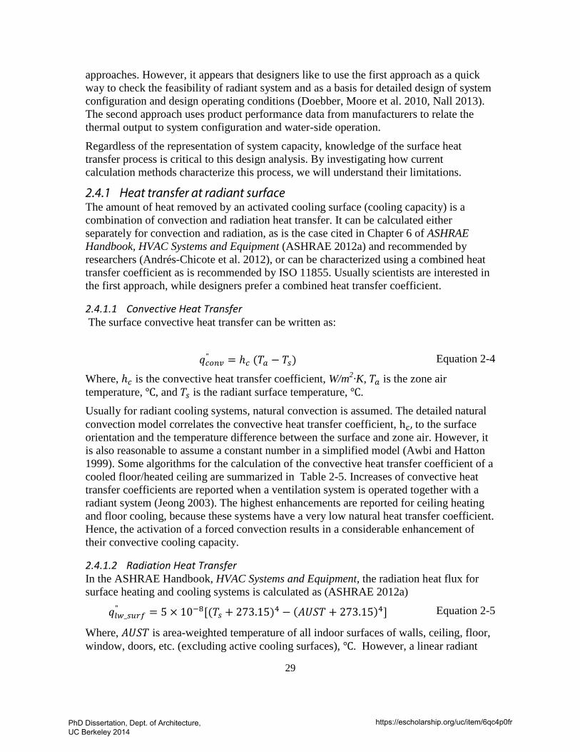
29

approaches. However, it appears that designers like to use the first approach as a quick way to check the feasibility of radiant system and as a basis for detailed design of system configuration and design operating conditions (Doebber, Moore et al. 2010, Nall 2013). The second approach uses product performance data from manufacturers to relate the thermal output to system configuration and water-side operation.

Regardless of the representation of system capacity, knowledge of the surface heat transfer process is critical to this design analysis. By investigating how current calculation methods characterize this process, we will understand their limitations.

2.4.1 Heat transfer at radiant surface The amount of heat removed by an activated cooling surface (cooling capacity) is a combination of convection and radiation heat transfer. It can be calculated either separately for convection and radiation, as is the case cited in Chapter 6 of ASHRAE Handbook, HVAC Systems and Equipment (ASHRAE 2012a) and recommended by researchers (Andrés-Chicote et al. 2012), or can be characterized using a combined heat transfer coefficient as is recommended by ISO 11855. Usually scientists are interested in the first approach, while designers prefer a combined heat transfer coefficient.

2.4.1.1 Convective Heat Transfer The surface convective heat transfer can be written as:

𝑞𝑞𝑐𝑜𝑛𝑣" = ℎ𝑐 (𝑇𝑎 − 𝑇𝑠) Equation 2-4

Where, ℎ𝑐 is the convective heat transfer coefficient, W/m2·K, 𝑇𝑎 is the zone air temperature, ℃, and 𝑇𝑠 is the radiant surface temperature, ℃. Usually for radiant cooling systems, natural convection is assumed. The detailed natural convection model correlates the convective heat transfer coefficient, hc, to the surface orientation and the temperature difference between the surface and zone air. However, it is also reasonable to assume a constant number in a simplified model (Awbi and Hatton 1999). Some algorithms for the calculation of the convective heat transfer coefficient of a cooled floor/heated ceiling are summarized in Table 2-5. Increases of convective heat transfer coefficients are reported when a ventilation system is operated together with a radiant system (Jeong 2003). The highest enhancements are reported for ceiling heating and floor cooling, because these systems have a very low natural heat transfer coefficient. Hence, the activation of a forced convection results in a considerable enhancement of their convective cooling capacity.

2.4.1.2 Radiation Heat Transfer In the ASHRAE Handbook, HVAC Systems and Equipment, the radiation heat flux for surface heating and cooling systems is calculated as (ASHRAE 2012a)

𝑞𝑞𝑙𝑤_𝑠𝑢𝑟𝑓" = 5 × 10−8[(𝑇𝑠 + 273.15)4 − (𝐴𝑈𝑆𝑇 + 273.15)4] Equation 2-5

Where, 𝐴𝑈𝑆𝑇 is area-weighted temperature of all indoor surfaces of walls, ceiling, floor, window, doors, etc. (excluding active cooling surfaces), ℃. However, a linear radiant



30

heat transfer coefficient can be defined to express the radiant heat exchange between a specific surface and all the other surfaces in the room.

𝑞𝑞𝑙𝑤_𝑠𝑢𝑟𝑓" = ℎ𝑟𝑎𝑑(𝑇𝑠 − 𝑇𝑟𝑒𝑓) Equation 2-6

Where, ℎ𝑟𝑎𝑑 is a linear radiant heat transfer coefficient, and can be considered constant and 5.5 W/m2.K is recommended (Olesen et al. 2000, ASHRAE 2012a). 𝑇𝑟𝑒𝑓 is a reference temperature that is not yet clearly defined, and it can be AUST or 𝑇𝑜𝑝𝑡 = the operative temperature at a reference point in the room, ℃. Both Eq. (2-5) and (2-6) are used only for characterizing longwave radiation heat transfer between the radiant cooling surface and its enclosure surfaces. The lack of consideration of the incident solar radiation and other internal heat gain on cooled surfaces was observed in calculation models documented in the guidelines and in several models developed by researchers.



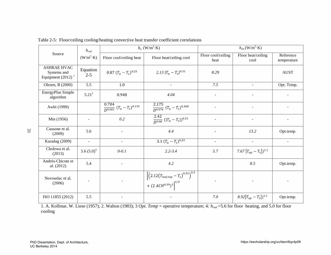
Table 2-5: Floor/ceiling cooling/heating convective heat transfer coefficient correlations

31

Source hrad

(W/m2·K)

ℎ𝑐 (W/m2·K) htot (W/m2·K)

Floor cool/ceiling heat Floor heat/ceiling cool Floor cool/ceiling heat

Floor heat/ceiling cool

Reference temperature

ASHRAE HVAC Systems and

Equipment (2012) 1

Equation 2-5 0.87 (𝑇𝑎 − 𝑇𝑠)0.25 2.13 |𝑇𝑎 − 𝑇𝑠|0.31 8.29 AUST

Olesen, B (2000) 5.5 1.0 - 7.5 - Opt. Temp.

EnergyPlus Simple algorithm 5.212 0.948 4.04 - - -

Awbi (1999) 0.704𝐷0.601 (𝑇𝑎 − 𝑇𝑠)0.133

2.175𝐷0.076 (𝑇𝑎 − 𝑇𝑠)0.308 - - -

Min (1956) - 0.2 2.42𝐷0.08 (|𝑇𝑎 − 𝑇𝑠|)0.31 - - -

Causone et al. (2009) 5.6 - 4.4 - 13.2 Opt.temp.

Karadag (2009) - - 3.1 (𝑇𝑎 − 𝑇𝑠)0.22 - - -

Cholewa et al. (2013) 5.6 (5.0)4 0-0.1 2.2-3.4 5.7 7.67 �𝑇𝑜𝑝 − 𝑇𝑠�)1.1

Andrés-Chicote et al. (2012) 5.4 - 4.2 8.5 Opt.temp.

Novoselac et al. (2006) - -

��2.12�𝑇𝑖𝑛𝑑,𝑡𝑜𝑝 − 𝑇𝑠�0.33�

0.3

+ (2 𝐴𝐶𝐻0.39)3�1/3

- - -

ISO 11855 (2012) 5.5 - - 7.0 8.92�𝑇𝑜𝑝 − 𝑇𝑠�)1.1 Opt.temp.

1. A. Kollmar, W. Liese (1957); 2. Walton (1983); 3 Opt. Temp = operative temperature; 4: hrad =5.6 for floor heating, and 5.0 for floor cooling



32

2.4.1.3 Total Heat Transfer To size HVAC systems, especially radiant systems, a combined coefficient is convenient. The key concept used to determine the cooling capacity in ISO-11855: 2012 is to “establish a basic characteristic curve for cooling and a basic characteristic curve for heating, for each type of surface, independent of the type of embedded system.” This means that a constant total heat transfer coefficient, depending on system type (floor/wall/ceiling and heating/cooling) is used to calculate the surface heat flux.

𝑞𝑞𝑡,𝑓𝑙𝑟" = ℎ𝑡𝑜𝑡(�𝑇𝑠 − 𝑇𝑟𝑒𝑓�) Equation 2-7

where, htot is the combined convection and radiation heat transfer coefficient, and its values are reported in Table 2-5. Again, only convection and longwave radiation between surfaces are included in the total heat transfer calculation, and solar/lighting/equipment radiation are not reflected.

2.4.2 Cooling capacity estimation method For manufacturers, methods documented in the standards are widely adopted to obtain radiant system capacity. For design engineers, there is no standardized way. A survey of leading designers indicated that the approaches include the direct use of numbers from the manufacturer’s product catalog, the use of designers’ in-house calculation tools, which are developed mostly for steady-state analysis, or conducting finite element or finite difference analysis, which allows for the evaluation of the system dynamic performance (Feng et al. 2014). Occasionally, the most experienced designers use whole building simulation software, such as EnergyPlus or TRNSYS to assist in design analysis. The use of these tools allows the evaluation of dynamic impacts from thermal loads and an assessment of control sequences. For the panel systems, the steady-state analysis method could be adequate because of the relatively small delay of the heat exchange between the environment and hydronic loop. For the embedded systems, a dynamic solution can be more desirable for improved prediction accuracy. It is, however, not widely achievable due to reasons such as lack of available skills or financial/time constraints. Simplified methods that are based on steady-state calculations are still the most widely adopted practice.

2.4.2.1 Standardized methods As mentioned before, most manufacturers reported radiant system capacity in correlation to a lumped thermal resistance, K, and a mean temperature difference between the cooling medium and the space, ∆𝑇ℎ. The mathematical format is as Eq (2-8).

𝑞𝑞" = 𝐾 ∙ ∆𝑇ℎ𝑛 Equation 2-8

Where, n is a constant, and is equal to 1 for the embedded systems according to ISO 11855. Both K and n are to be determined. The parameters that are included in the resistance, K, are surface heat transfer coefficients, resistance of the radiant conductive layers, resistance between water loop and pipe, etc. According to Zhang (Zhang et al. 2012), the surface heat transfer coefficient is the most significant parameter among all other thermal resistances lumped in K.



33

Definitions and determinations of the four parameters in Eq.(2-8) depend on system types and applications (see Table 2-6). The basic concepts are, as stated in ISO 11855:

“A given type of surface (floor/wall/ceiling) delivers, at a given average surface temperature and indoor temperature (operative temperature), the same heat flux in any space independent of the type of the embedded system. It is therefore possible to establish a basic formula or characteristic curve for cooling and a basic formula or characteristic curve for heating, for each of the type of surfaces, independent of the type of embedded system.”

An example of a diagram with the characteristic curves generated by a well-known radiant slab manufacturer is presented in Figure 2-5. ASHRAE Handbook recommends similar types of diagram for the estimation of thermal output of radiant systems. It can be useful for designers to have an idea of what kind of radiant systems they are looking for in order to achieve desired thermal performance

To obtain such characteristic curves, either testing or calculation methods can be used (see Table 2-6). Testing methods involve evaluating radiant system performance by conducting laboratory testing following the procedure prescribed in standards, and calculation methods involve estimating system capacity using analytical or numerical methods. For radiant panel systems, only testing methods are permitted (ASHRAE 138/EN 14240 for cooling and EN 14037 for heating), while for embedded systems, both calculation and testing methods are permitted. However, the testing method for embedded systems, the “two plate” method described in EN 1264, only applies to floor heating systems. If performance data is desired for cooling application or other surfaces (wall/ceiling), a conversion factor has to be applied (see Table 2-6). This conversion factor accounts for difference in surface heat transfer coefficients for cooling/heating (wall/ceiling) applications and surface covering thermal resistance.



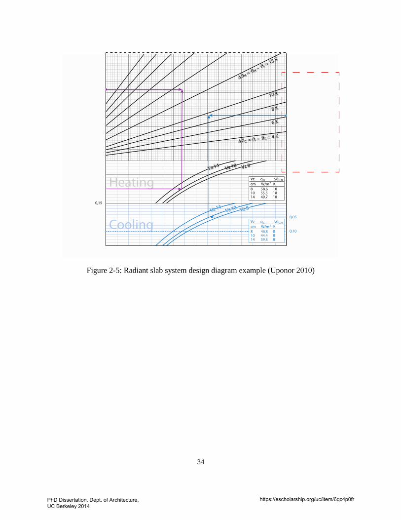
34

Figure 2-5: Radiant slab system design diagram example (Uponor 2010)



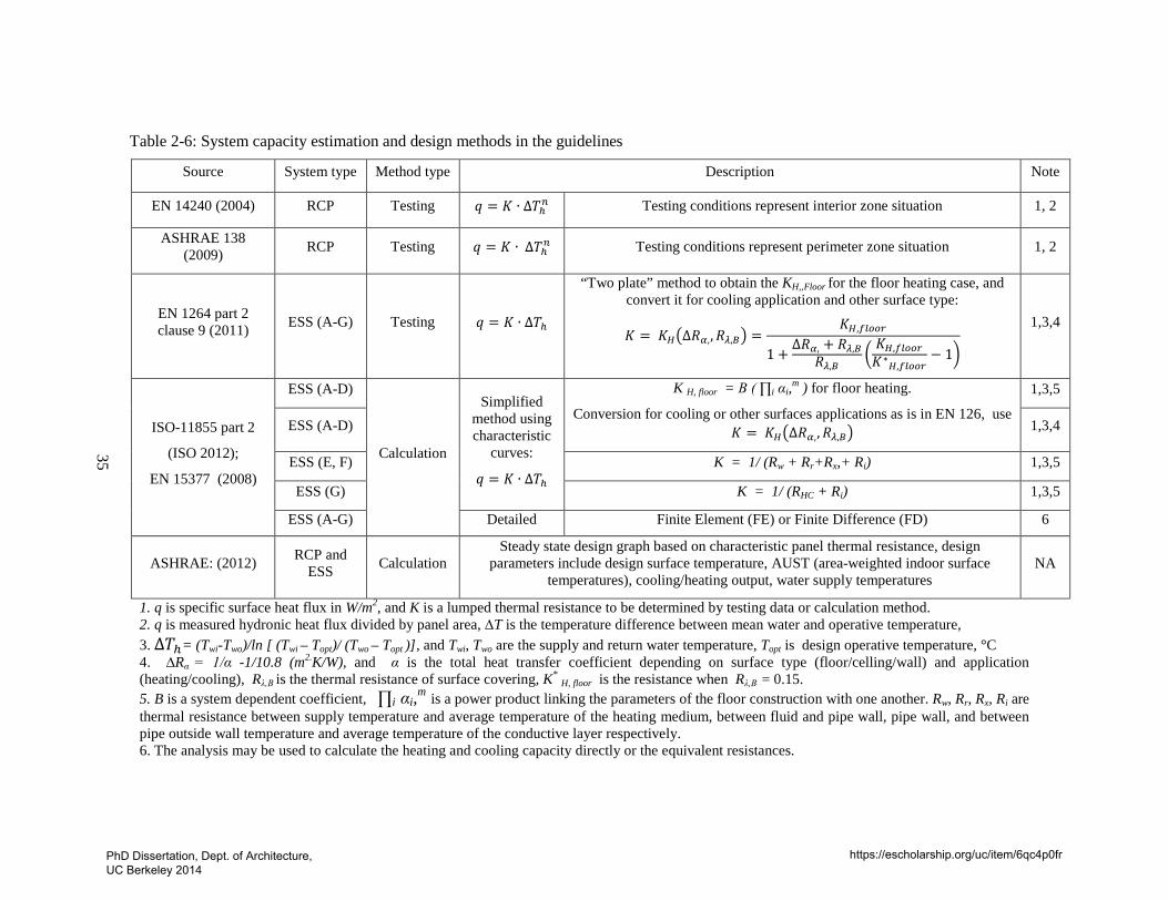
Table 2-6: System capacity estimation and design methods in the guidelines

35

Source System type Method type Description Note

EN 14240 (2004) RCP Testing 𝑞𝑞 = 𝐾 ∙ ∆𝑇ℎ𝑛 Testing conditions represent interior zone situation 1, 2

ASHRAE 138 (2009) RCP Testing 𝑞𝑞 = 𝐾 ∙ ∆𝑇ℎ𝑛 Testing conditions represent perimeter zone situation 1, 2

EN 1264 part 2 clause 9 (2011) ESS (A-G) Testing 𝑞𝑞 = 𝐾 ∙ ∆𝑇ℎ

“Two plate” method to obtain the KH,,Floor for the floor heating case, and convert it for cooling application and other surface type:

𝐾 = 𝐾𝐻�∆𝑅𝛼,,𝑅𝜆,𝐵� =𝐾𝐻,𝑓𝑙𝑜𝑜𝑟

1 +∆𝑅𝛼, + 𝑅𝜆,𝐵

𝑅𝜆,𝐵�𝐾𝐻,𝑓𝑙𝑜𝑜𝑟𝐾∗

𝐻,𝑓𝑙𝑜𝑜𝑟− 1�

1,3,4

ISO-11855 part 2

(ISO 2012);

EN 15377 (2008)

ESS (A-D)

Calculation

Simplified method using characteristic

curves:

𝑞𝑞 = 𝐾 ∙ ∆𝑇ℎ

K H, floor = B ( ∏i αi,m ) for floor heating.

Conversion for cooling or other surfaces applications as is in EN 126, use 𝐾 = 𝐾𝐻�∆𝑅𝛼,,𝑅𝜆,𝐵�

1,3,5

ESS (A-D) 1,3,4

ESS (E, F) K = 1/ (Rw + Rr+Rx,+ Ri) 1,3,5

ESS (G) K = 1/ (RHC + Ri) 1,3,5

ESS (A-G) Detailed Finite Element (FE) or Finite Difference (FD) 6

ASHRAE: (2012) RCP and ESS Calculation

Steady state design graph based on characteristic panel thermal resistance, design parameters include design surface temperature, AUST (area-weighted indoor surface

temperatures), cooling/heating output, water supply temperatures NA

1. q is specific surface heat flux in W/m2, and K is a lumped thermal resistance to be determined by testing data or calculation method. 2. q is measured hydronic heat flux divided by panel area, ∆T is the temperature difference between mean water and operative temperature, 3. ∆𝑇ℎ= (Twi-Two)/ln [ (Twi – Topt)/ (Two – Topt )], and Twi, Two are the supply and return water temperature, Topt is design operative temperature, °C 4. ∆Rα = 1/α -1/10.8 (m2.K/W), and α is the total heat transfer coefficient depending on surface type (floor/celling/wall) and application

(heating/cooling), Rλ,B is the thermal resistance of surface covering, K* H, floor is the resistance when Rλ,B = 0.15. 5. B is a system dependent coefficient, ∏i αi,m is a power product linking the parameters of the floor construction with one another. Rw, Rr, Rx, Ri are

thermal resistance between supply temperature and average temperature of the heating medium, between fluid and pipe wall, pipe wall, and between pipe outside wall temperature and average temperature of the conductive layer respectively.

6. The analysis may be used to calculate the heating and cooling capacity directly or the equivalent resistances.



36

2.4.2.2 Methods in research world Besides the methods described in standards, modeling of radiant systems is a popular topic in the research world.

For radiant panel systems, the earliest study on modeling of the radiant heating system may date back to the 1970s, and was conducted by Hedgepeth and Sepsy (1972). They developed the complex thermodynamic model of a heating panel consisting of copper tubes and square aluminum fins as ceilings at steady-state conditions to evaluate the heat rejection rate. This model was integrated with the pump subsystem and a transient load calculation technique to simulate the system operation of the radiant-panel heating system. Such a simulation package was validated using an experiment of the radiant-panel heating system (Johes al. 1975). More recent studies (Jeong and Mumma (2004), Fonseca (2011)) focus on environmental impacts (air velocity, heat source in the space) on surface heat transfer rate.

For embedded systems, besides the simplified models provided in ISO 11855, there are also many research papers on this topic. In the 1990s, a steady-state fin model was proposed for modeling the heat transfer of the pipe-embedded structure by Kilkis (1993). This model treats the radiant and convective heat output separately. The required floor surface temperature and the required mean water temperature for meeting the heating demand are expressed in the algebraic form with respect to physical properties and geometric dimension of the structure, etc. Iteration is required to obtain the final output. This model was validated using the numerical solution of the structure by using a finite element package (Kilkis et al. 1995). Kilkis and Sapci (1995) further developed the heat transfer model of a subfloor where the pipes with hot water passing through is attached from the joist space. Then, this subfloor heat transfer model was integrated with the hydraulic system and the room model, etc., resulting in an interactive computer program for optimizing the mean water temperature and the tube cost. Based on the steady-state fin model, Kilkis and Coley (1995) also developed complete design software for pipe-embedded structures, such as floors/ceilings, for predicting the heat rejection of the structure and other performance. At the same time, a universal design monograph is presented for manual design of the pipe-embedded structure for ceiling/floor panel heating. The research projects presented by Kilkis et al. are meaningful and resulted in a design software and universal design monograph for hot water panel heating. However, the model is steady state, and it cannot be used to assess the transient thermal performance of a pipe-embedded structure for air-conditioning.

Antonopoulos (1992) developed a one-dimensional steady-state analytical model for temperature field analysis on the cooling panel. The one-dimensional model is easy to apply in practice. However, this model is steady state, and cannot be used for transient thermal performance analysis of pipe-embedded structure for air-conditioning that depends on concrete mass for thermal (cool/heat) storage where a transient state dominates. The researchers also presented two- dimensional and three-dimensional steady and transient models (Antonopoulos and Democritou 1993, Antonopoulos and Tzivanidis 1997a) and evaluated those model by full-scale experiments (Antonopoulos, Vrachopoulos et al. 1997b). These models need to be solved numerically and can provide



37

quite accurate solutions. However, they are time consuming and often cause stability problems if they are linked to other components in a simulation environment (Weber and Johannesson 2005).

Strand and Baumgartner (2005) used the transfer function description to describe the heat transfer of the pipe-embedded structure resulting in the heat source transfer function. This function includes the effect of the thermal source/sink in this structure, and was obtained through both the Laplace transform method and the state space method, which could be adapted to two-dimensional solutions. The source transfer function was validated using the analytical solution and experimental data of this structure. This model was integrated with the Integrated Building Loads Analysis and System Thermodynamics (IBLAST) program as an engineering tool for researchers and designers for evaluating the performance of this active pipe-embedded structure. The model was also implemented in EnergyPlus by adding a heat source term in the transfer function (DOE 2011). However, the main drawback of the transfer function, as pointed out by Weber and Johannesson (2005), is the linking to non-linear processes, such as changing mass flow in the pipe when compared with a RC-network. As a consequence, the heat exchange at the pipe is modeled as a heat exchanger having a fluid on one side and a stationary fluid with uniform temperature along the pipes. The assumption of having uniform temperature along the pipes stems from an assumption in the derivation of the transfer function. This means that it is not possible to include such a transfer function formulation to a simultaneous heat transfer calculation along a pipe with temperature drop and changing fluid flow. The two components can only be calculated separately from each other.

Koschenz and Dorer (1999) presented a simplified steady-state model of an active pipe-embedded structure for air-conditioning in which the slab with water pipes embedded was modeled as two “walls”, separated by a dummy zone representing the water system with heat transfer coefficients according to resistances. Both sides of this slab are not insulated with one side as the floor and the other side as the ceiling. The required water temperature for cooling can be calculated based on this steady-state model when the load profile of this space and the physical properties of the slab, etc., are specified. The rise of the water temperature in the pipe can be estimated approximately by using the logarithmic average method on the basis of the room air temperature. This simplified model was integrated with the building and system simulation program TRNSYS. This model was roughly validated by comparison with the simulation results from the finite element calculations of this structure.

In 2005, Weber and Johannesson (2005) presented a simplified RC-network model for an active pipe-embedded structure (called a “thermally activated building component system (TABS) in this article). This model was validated by comparing its predictions with detailed in situ measurements in an office building using the structure as floors. The structure was equipped with 80 measurement points including temperature measurements at different heights of the slab as well as in the suspended floor and in both adjacent rooms, the supply and return water temperatures, the volume flow, and the heat flow at the surface of the concrete slab. These measurements were also used to validate a FEM-program (finite element method) working in frequency domain (Weber et al. 2005). It



38

appears that a simplified RC model is the best candidate for modeling an active pipe-embedded structure since it can simulate the dynamic thermal process in the structure and it can be solved easily for convenient integration with energy simulation software. However, not much detail on the parameter determination of this RC model is presented since these parameters have a significant effect on the thermal performance of this structure.

2.4.3 Summary and questions In summary, there is a wide range of approaches for modeling, and thus predicting, the heat transfer process within the radiant layers. Even though there are issues associated with each modeling method, most models can predict the heat transfer process within the radiant layers with acceptable accuracy. The issue that is missing is the dynamic coupling between radiant surfaces and its environment plus various heat sources. To evaluate this, a radiant system model needs to be integrated into conventional building energy simulation packages. Multiple-dimensional numerical transient or steady-state models of the active pipe-embedded structure may be integrated with conventional building energy simulation packages. However, there are still many challenges in the process. For example, the computation demand is large, and the whole simulation may become unstable when the numerical model is linked to other components in the simulation environment (Fort). Thus, integrated simulation of a radiant slab model with a whole environmental tool is not commonly adopted. Instead, steady-state models were widely used (see section 2.6). Even if the dynamic models are used for the analysis, the radiant surface boundary conditions are simplified, taking into account only convection heat transfer and the longwave radiation between surfaces. Radiant exchanges from internal and solar gains are ignored. This explains why there are many occasions, as described in section 1.3.2, when the standardized method cannot predict system capacity well.

2.5 Control for thermally active building systems

2.5.1 Literature review In the literature, some early reports on rule based control methods for thermally active building systems include Olesen (Olesen 1997a, Olesen 2001) and Weitzmann (2004), the latter giving a short overview of proposed control-concepts. Some common properties of the algorithms include: (a) adjustment of water supply temperature set point is a function of outside air temperature; (b) self-regulation of the concrete slab conditioning system is assumed to be sufficient; and (c) heating and cooling operation are enabled or activated depending on the season and/or outside air temperature. These rule-based control models have been mostly derived empirically from simulations or steady-state physical models so it is hard to expand their applicability.

Olesen et al. (2002) has evaluated some of the commonly used control methods by parametric study using TRNSYS. The control methods they studied include time of operation intended to take advantage of nighttime precooling, intermittent operation of a circulating pump intended to reduce pump power, and control of water temperature intended to maintain stable indoor air temperature and utilize the self-control capability of slab system. Their simulation results verified some general rules that can achieve



39

energy savings and thermal comfort, such as controlling water temperature as close as possible to room temperature to prevent overcooling or overheating and operating pumps intermittently. They also concluded that the best comfort and energy performance is obtained by controlling the water temperature (supply or average) as a function of outside temperature. However, the study was conducted for a prescribed building construction in one single climate, and therefore, it is hard to generalize the results for different buildings in different climates.

As discussed in Section 1.3.3, control of thermally active building systems is a complex issue, and it is challenging for the traditional heuristic rule-based control methods to successfully tackle it. Therefore, there is a need to investigate the possibility and potential benefits of using advanced control techniques.

A more advanced control method was developed by Gwerder, et.al, who proposed a pulse-width modulated (PMV) intermittent operation of water circulation pump, combined with supply water temperature control (Gwerder et al. 2008, Gwerder et al. 2009, Lehmann et al. 2011). Their method aimed to take into account uncertainties in load disturbance when achieving both comfort criteria and energy efficiency. However, there is no documentation on the application or validation of their method.

More recently, model predictive control (MPC) has become popular in the building industry (Ma et al. 2012, Oldewurtel et al. 2012, Hu and Karava 2014). MPC is a flexible and well-developed advanced control technique with broad applications in complex systems. Its optimization and prediction features make it particularly advantageous in the application of radiant slab systems. Gayeski (2010) presented a study focused on optimizing the control of a low-lift chiller serving a radiant slab system. The energy consumption of the cooling system, including chiller, compressor, condenser fan, and chilled water pump, was minimized. Corbin et al. (2012) have developed a model predictive control (MPC) environment integrating Matlab and EnergyPlus to predict optimal building control strategies. The environment is used to determine hourly supply water temperature and circulator availability that minimize daily energy consumption for a small office building having a radiant slab system. One common feature of these methods is high computational requirements due to model complexity. Practitioners perceived this as a major obstacle in terms of the applicability and scalability. To reduce the computational intensity during online operation, Coffey (2011) proposed a method of using a look-up table to obtain near optimum control decisions. The look-up table is pre-generated with a Model Predictive Controller. They demonstrated its application to the control of an abstract single zone radiant cooling system. May-Ostendorp et al. (2013) investigated the performance of MPC based rules in a test cell. MPC was first used to identify combined radiant slab systems and ventilation control strategies that maximized cooling energy savings while preserving thermal comfort. A rule extraction process using classification and regression trees then yielded supervisory rules capable of reproducing nearly all of the energy and comfort benefits of the model predictive control solutions when simulated. The experiment yielded 40% average cooling energy savings compared to a base case, with comparable comfort.



40

2.5.2 Summary In summary, more advanced control methods for radiant slab systems are needed, and MPC is a promising technique. However, current models are complicated for real time MPC implementation, and rule extraction technique has to be applied. Thus, the question is whether it is possible to create a simplified dynamic model of a radiant slab system for easy implementation in a model predictive controller. More importantly, there is a need for demonstration of the application of MPC to real buildings to show the long-term energy and comfort benefits.

2.6 State of art of the design industry

2.6.1 Survey and interview To assess the state of the art of the industry, surveys and interviews of leading practitioners and manufacturers were conducted. The survey consisted of four open-ended questions, investigating the adaptation of standard methods in the design community; identifying the range of approaches used in practice, adding observational information about design process, and understanding the tool selection criteria (see Table 2-7 for questions asked). In concert with the survey, interviews were conducted through email, face-to-face communications, or a combination thereof. Interviewees included: 1) some of the survey respondents, in order to confirm and clarify their answers and to follow-up with more detailed questions; 2) authors of publications that have described radiant system design approaches or specific projects; and 3) designers who have extensive experience working on radiant projects. Besides the questions Q 1-4 listed in Table 2-7, Q5-8 are other questions asked in the interviews, which were about the general design process, the role of different design parties, and their experiences with the tools they used.

The survey was deployed in August 2012 via email to twenty design practitioners, manufacturers, and top researchers who are experienced with radiant systems. In total, I had twelve respondents. Eight interviews were conducted.



41

Table 2-7: Survey questions

Q1: How do you calculate the cooling load of the spaces conditioned by a radiant cooling system? Which tools do you use?

Q2: How do you size the radiant slab system? For example, based on 24-hour total cooling load, peak cooling load, average cooling load during operating hours or others?

Q3: How do you estimate radiant cooling system capacity? Which tools do you use?

Q4: How do you handle cases with the presence of high solar heat gain (skylight, atria, perimeter zones, etc.)?

Additional questions asked during interview (the questions listed below were not asked to every interviewee)

Q5: Can you describe the standard or general design process of a radiant project?

Q6 What’s the role of whole building simulation in the design process?

Q7: What’s the role of each design party (MEP, radiant system subcontractor/consultant, manufacturers or their representatives, energy consultants, architects, modelers, etc.)?

Q8: What’s your experience with the design tools you used?

Results from question 1 (see Figure 2-6 ) show that 31.8% of the respondents use tools that employed simplified ASHRAE load calculation methods (e.g., RTS/Transfer function methods), 27.3% use steady-state heat gain as cooling load. It is also important to realize that even though some tools have been reported being used, it does not necessarily mean that those tools were used for all radiant projects the respondents have worked on. Thus even though 22.7% of the respondents reported using dynamic simulation tools that calculate space load based on heat balance methods and are capable of modeling radiant systems, interview results indicated that those tools are generally perceived as complicated and too time and cost consuming to be used in most projects.

For question 2 (see Figure 2-7 ), 71.4 % of the respondents reported that peak cooling load was used for sizing a radiant slab system. Two respondents also indicated that the capacity of a radiant system is too low compared to the total cooling load, so they always size the radiant systems only to meet a constant base load based on a rule of thumb for maximum radiant system cooling capacity (Olesen 2008), and size the associated air system to meet the fluctuating load. Two other respondents mentioned that they used steady-state average cooling load for sizing slab systems, which is consistent with the design concept proposed in ISO 11855.

For question 3 (see Figure 2-8 ), besides commercially available dynamic simulation software, more than 46% of the respondents indicated that steady-state analysis was conducted in radiant system design process, which was assisted by tools that are based on the ISO 11855 simplified method, or finite element/difference methods, or other algorithms. Respondents who reported using methods based on ISO 11855 were mostly manufacturers.



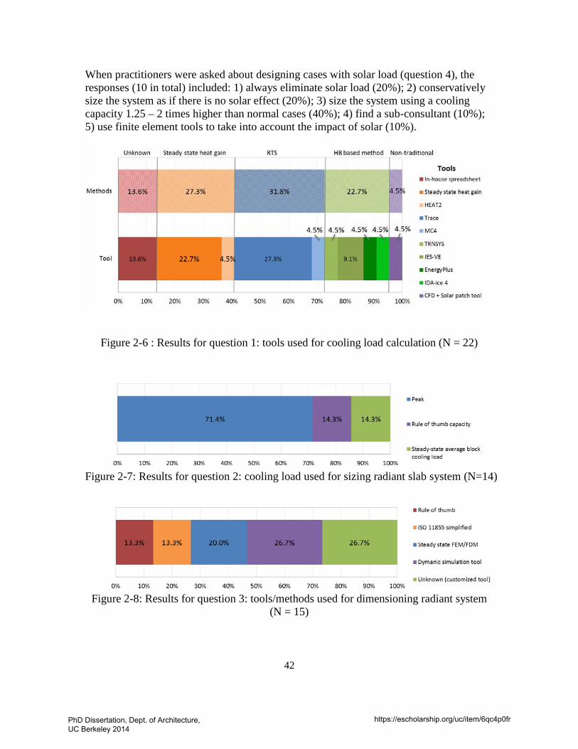
42

When practitioners were asked about designing cases with solar load (question 4), the responses (10 in total) included: 1) always eliminate solar load (20%); 2) conservatively size the system as if there is no solar effect (20%); 3) size the system using a cooling capacity 1.25 – 2 times higher than normal cases (40%); 4) find a sub-consultant (10%); 5) use finite element tools to take into account the impact of solar (10%).

Figure 2-6 : Results for question 1: tools used for cooling load calculation (N = 22)

Figure 2-7: Results for question 2: cooling load used for sizing radiant slab system (N=14)

Figure 2-8: Results for question 3: tools/methods used for dimensioning radiant system

(N = 15)



43

2.6.2 Case studies Design methods/process/tools used in the industry are a mixture of “rule of thumb” and steady-state or dynamic analysis. To put this in a concrete context, I described the design process of some selected projects that cover applications characterized by different load conditions, applications and, thus, challenges. Accessibility to detailed design information was another factor affecting the selection. Even though there are numerous case study papers on radiant projects, most of them only provided general information, or only focus on particular design/control strategies. The information presented here is collected from published papers, websites, internal reports, direct communication with project designers, or a combination thereof.

2.6.2.1 Wal-Mart, Sacramento, California A radiant floor cooling system combined with a DOAS was designed and installed in a Wal-Mart in Sacramento, CA in June 2009. The design for this large retail store was assisted by standard design practices, whole-building energy simulation, and finite element analysis. Information about this project was obtained from a paper by Ian Doebber (2010) and personal communication with the author.

A whole building simulation tool, EnergyPlus, which is based on the heat balance method, was used to assist with various design studies, from the decision of whether a radiant floor was a viable option to the evaluation of different control sequences. The designers used EnergyPlus because they believed that the capability of capturing transient convective and radiative heat transfers between the space and the radiant floor was critical.

During the feasibility study, initial load calculations indicated the peak sensible cooling load would be less than 50.5 W/m2, which is within the range of radiant floor cooling.

During the detailed design stage, EnergyPlus was used to generate the design sensible load profile, and the radiant floor was simulated during the process. With a peak cooling load at 49.8 W/m2, a required radiant floor surface temperature was determined to be 18.9 °C. This is obtained by assuming 8 W/m2·K total floor heat transfer coefficient, 24.4 °C space dry bulb and 25.6 °C roof/wall surface temperature.

In the next step, the designers aimed to configure the floor to meet the peak cooling rate. The design team first came out with a design, including tube spacing, tube diameter, tube length, tube depth, slab thickness, and insulation, using standard design practice assisted by a computer program like RadiantWorks (http://www.wattsradiant.com/support/radiantworks/). Slab thickness and insulation effect were further evaluated with an EnergyPlus simulation to finalize the design. Design water flow rate was determined to be 2.8 °C (rule of thumb range is 2.8 to 5.0 °C) to maximize waterside economizing at the expense of increased pumping energy. With the aforementioned design parameters fixed, a steady-state finite element analysis calculated a 14.4 °C supply and 17.2 °C return would maintain a 18.9 °C floor surface temperature while providing a 49.8 W/m2 cooling rate.

Due to the structure of the project, another design company was hired to evaluate the design by integrating it into a calibrated IES-VE model, and they looked at the energy



44

implications of the design. This IES-VE model was used for exploring various control strategies. After much iteration, building simulations predicted that a variable flow-variable temperature strategy would provide the best performance, and a linear chiller supply water reset schedule was developed to mitigate peak cooling demand.

The IES-VE model compared annual electrical energy consumptions of various design alternatives and control strategies. The design with radiant floor combined with DOAS system using variable-flow, variable-supply water temperature control can save up to 58% compared to a standard efficiency constant air volume DX rooftop unit design.

In general, the design process for this Wal-Mart can be summarized as below:

• Used a dynamic tool that employed heat balance method to determine peak cooling load.

• Modeled a radiant system during the design process, so that the interactions between the cooled floor surface and space load could be captured during load analysis.

• Configured a floor system capable of removing peak cooling rate. The design team used standard design practice in combination with steady-state finite element calculation and dynamic simulation in this process.

• Developed a control strategy, assisted by dynamic simulation, which could leverage the thermal mass for demand management.

In this project, EnergyPlus was chosen intentionally because the designers recognized that being able to capture the convective and radiative (both longwave and shortwave) interactions between the radiant floor and its surroundings are critical for system sizing purpose. Also, at least two energy models were developed for the design, an EnergyPlus model was used for load analysis and radiant system design, and an IES-VE model was used for control development and whole system energy evaluation as compared to other design alternatives. An IES-VE model was used because the company that was hired to evaluate the design had the required skill and was familiar with the tool.

2.6.2.2 David Brower Center, Berkeley, California The David Brower Center (DBC) is a four-story 4,042 m2 office building located in downtown Berkeley, California. The building was completed and first occupied in 2009. It contains a lobby and public meeting space on the first floor and open-plan office spaces on the second through fourth floors, which primarily house nonprofit environmental activist organizations. Design information about this project was obtained from documents provided by mechanical designers and interviews.

The radiant slab ceiling system design process was similar to the Wal-Mart project. The mechanical design team used TRANE TRACE for thermal load analysis. Since this software does not have the capability to model embedded radiant systems, the radiant effect of the cooled/heated surface was ignored during the load calculation stage. TRANE TRACE offers several load calculation methodologies, including the RTS and some other transfer function methods, which are all simplified calculation methods



45

With the peak cooling/heating load provided by the MEP, a radiant slab manufacturer’s representative provided detailed radiant system design specifications, including tube type, number of loops required, tube length, pressure loss, design surface temperature and supply water temperature, and design water flow rate. The design was generated by Uponor’s Advanced Design Suite TM software, which employs the ISO 11855 cooling/heating capacity calculation method.

The whole-building simulation tool, eQUEST, was used to perform annual energy and comfort analysis for code compliance. The radiant slab system was simulated in eQUEST as a fan coil system with fan power reset to zero.

The original rule-based control sequence was developed by the MEP firm, and the systems were adjusted by the operating staff and MEP firm in the first couple of years of operation, and by 2012, the building was operating as intended with a high level of occupant satisfaction level in terms of thermal comfort, air quality, lighting, etc.

In general, the design process and tools involved in the Brower Center are summarized below:

• A thermal load study was conducted using a dynamic load calculation tool that uses RTS or TF methods;

• Radiant effect created by the cooled/heated surface was not considered during load calculation process;

• The detailed slab design was generated by a manufacture developed tool based on the ISO 11855 cooling/heating capacity calculation method.

The design tools, eQUEST, used in this project and the work-around method for modeling radiant systems are typical practices in the United States according to interviews with designers from major design companies. TRACETM 700 was considered the best practice for load calculation.

2.6.2.3 Hearst Corporation Headquarters Lobby, New York Radiant floor cooling systems are increasingly being used in transitional spaces with large glazed surfaces, such as atria, airports, and perimeter areas. The lobby of the Hearst Corporation Headquarter in New York is an example of such application.

The Hearst Corporation Headquarters in New York was designed by Lord Norman Foster, and incorporates a multi-story lobby that is wrapped by the historic façade of the existing Hearst building. Extensive skylights and clerestories provide not only daylighting but also significant solar heat gain to the space. Radiant heating/cooling along with displacement ventilation provides the entire environmental control for this almost 3,000 m2 space (Nall and Ellington 2001).

The design process was accomplished using five tools (Nall 2013). First, given the dominant impact of solar load on radiant system performance, a tool that can calculate the pattern of solar irradiation on building surfaces at various times of the year provided absorbed solar heat flux data at each surface. These fluxes were used as input to a floor system evaluation tool in Engineering Equation Solver (EES).



46

A proprietary EES tool with an algorithm similar to the ISO 11855 methods allows the evaluation of alternatives in floor finish conductance, slab depth, tubing loop length, design water flow rate and temperatures for different combinations of room temperature and absorbed solar flux on the floor. The EES method does a heat balance at the floor surface, taking into account a specified combined radiant/convective film coefficient for the floor surface. An equilibrium floor temperature is iteratively calculated, along with the cooling or heating capacity of the floor per unit area.

The solar heat flux from the first tool was also fed into the computational fluid dynamics (CFD) tool, which evaluates room level heat transfer for the space and the impact of the ventilation supply air on the air temperature distribution in the space.

The fourth tool provided validation of psychometric balance in the space.

And the final tool for application to the system was a standard building energy modeling platform. Communication with the designer confirms that eQUEST was the most common tool they used to perform this task, and workarounds were required to capture the performance properly.

In short, the design process and tools involved in this project can be summarized as below:

• They explicitly located where the solar heat gain is absorbed for the determination of zoning and floor system design

• A proprietary EES tool was developed for the radiant system design.

• Ventilation system design was assisted by CFD analysis

• A psychometric analysis was performed to further validate the design

• A whole-building simulation tool, eQUEST, was used to perform annual energy and comfort analysis for code compliance.

In this project, solar pattern (intensity and path) was carefully understood because radiant floor performance is highly influenced by shortwave radiation, and such information was critical for system zoning and system configurations. Since solar load was dominant in this project, a conventional load calculation procedure was not conducted. In addition, CFD was used because thermal stratification and ventilation distribution patterns are critical features in applications in large space with solar load.

2.6.3 Summary In summary, there is a wide range of design and operating solutions in practice. Current design guidelines provide some principles for design analysis, but there is a lack of guidance on how to apply the principles to practice and on the selection of tools.

Most practitioners calculate the cooling load for radiant systems the same way as for air systems, with only 22.7% of the respondents reported using dynamic simulation tools that have the capability to model radiant systems for cooling load estimation.

For radiant system sizing, 46% of the respondents reported that steady-state analysis methods/tools were used. Whole building simulation tools that have the capability to



47

model radiant systems, such as EnergyPlus or TRNSYS, are not commonly adopted for the purpose of system sizing or annual performance evaluation.

Designing for a floor system when solar load is dominant is a challenge. The process reported in the case study was provided by one of the most experienced designers in North America, and feedback from most designers indicated that they regarded his method as impractical or too complicated for wide adoption.

2.7 Conclusions Through literature review, twelve surveys and eight interviews with leading practitioners, and three case studies, this chapter summarizes the design methods documented in the guidelines, assesses the state of the industry, and identifies potential gaps and limitations in current design and control practice. Here are some highlighted trends and issues.

For cooling load analysis, ASHRAE standards define a universal cooling load definition and provide detailed load calculation methods that apply to any HVAC system, while European or ISO standards, without suggesting detailed methods, imply that definition and methods may depend on system types, operating hours, and temperature control strategy. In the surveyed design community, 31% of the respondents reported using tools that employed the RTS method when designing radiant systems and 27% considered steady-state calculation of heat gain to be sufficient. This means most practitioners calculate cooling load for radiant systems the same way as for air systems. Even though 22.7% of the respondents reported using dynamic simulation tools that calculate space load based on heat balance methods and are capable of modeling radiant systems, those tools are generally perceived as being complicated, time consuming and high cost. Thus, there is a need to improve understanding about the differences between the two systems and provide guidance on load analysis and modeling methods.

For radiant system design, there is a wide range of approaches for modeling and sizing of both radiant panel and embedded systems. Most methods do not capture well the radiation coupling between radiant surfaces and its environment and various heat sources. One example is when calculating surface heat transfer coefficients, only natural convection and longwave radiation between active surfaces and other surfaces are considered and radiant exchanges from internal and solar gains are ignored. This results in many questions for practitioners when designing a system in a space that has a large solar load (shortwave radiation). Research is needed to quantify the impacts, understand the design implications, and improve the current calculation methods.

Control is not generally considered during system sizing analysis, but may be analyzed for whole system performance evaluation. Rule based control methods are dominant in the industry. Advanced control methods for radiant slab systems that can be easily implemented in practice are needed. In general, designers and operators are hesitant to implement more advanced control methods, and verification of the benefits by using real projects can facilitate the adoption of advanced control techniques.



48

3 COMPARISON OF COOLING LOADS BETWEEN RADIANT AND AIR

SYSTEMS-----SIMULATION STUDY

3.1 Introduction Cooling load calculations are a crucial step in designing any HVAC system. The objectives of this chapter are to use simulation to assess the cooling load differences between a radiant cooling system (with activated chilled surface) and an air system by comparing the zone level peak cooling load and 24-hour total cooling energy.

3.1.1 Radiant vs. air systems A comparison between radiant and air systems is challenging. In this section, I discuss the differences between the two systems that dictate the modeling approach used in this study. Besides those mentioned in the literature (Fabrizio et al. 2011), the main difficulties include:

• Types of load (sensible/latent) and the expected amount of load to be handled by the two systems are different. Air systems are usually designed to be the only system to handle both latent and sensible loads, while radiant systems must operate in hybrid mode with an additional reduced-sized air system (for ventilation and latent loads). Radiant cooling systems are always sized to handle a portion (as much as possible) of the sensible-only cooling load. To address this issue, neither the latent load nor ventilation system was simulated. This was to simplify our analysis.

• The design cooling load concept is different for the two systems. As discussed in section 2.3, the sensible cooling load for an air system is calculated in terms of maintaining a constant zone air temperature, while radiant systems, particularly TABS, are not capable of maintaining a constant zone air temperature due to the large thermal inertia of the active surfaces. For this reason, in this comparison study, I sized and controlled the simulated radiant systems to maintain an acceptable thermal comfort range during the simulation period. Operative temperature was used as the control temperature for both systems (Babiak 2007, Fabrizio et al. 2011). To ensure equivalent comfort conditions between the two systems for fair comparison, all simulations of the air system were subsequently controlled to closely track the hourly operative temperature profile derived from the radiant system simulation for the identical input conditions.

3.1.2 Cooling load at radiant surface and hydronic level For an air system the zone level cooling load is equal to the heat extraction rate by the mechanical system when the room air temperature and humidity are constant. But this is not always the case in a radiant system. Other than panel systems, the thermally massive radiant cooling systems (ESS and TABS) are integrated with the building structure with hydronic pipes embedded in the mass. As a result, heat removed from the zone at the chilled surface can be quite different from the heat removed by the hydronic loop. This



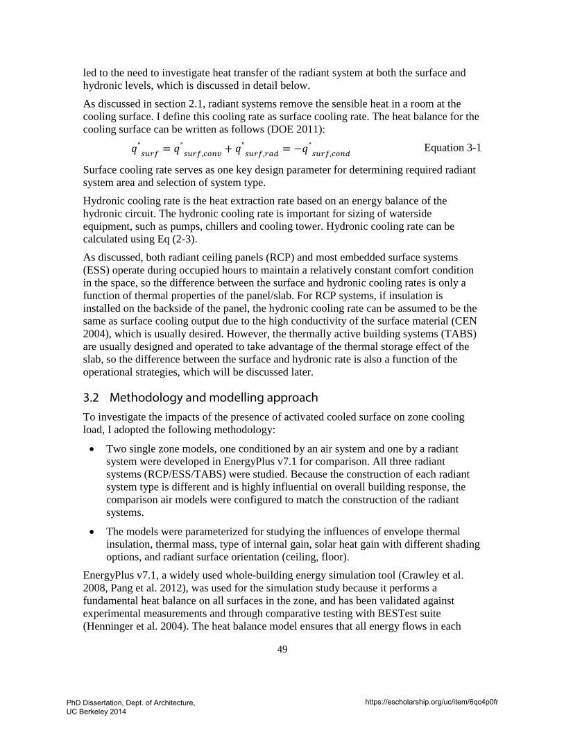
49

led to the need to investigate heat transfer of the radiant system at both the surface and hydronic levels, which is discussed in detail below.

As discussed in section 2.1, radiant systems remove the sensible heat in a room at the cooling surface. I define this cooling rate as surface cooling rate. The heat balance for the cooling surface can be written as follows (DOE 2011):

𝑞𝑞"𝑠𝑢𝑟𝑓 = 𝑞𝑞"

𝑠𝑢𝑟𝑓,𝑐𝑜𝑛𝑣 + 𝑞𝑞"𝑠𝑢𝑟𝑓,𝑟𝑎𝑑 = −𝑞𝑞"

𝑠𝑢𝑟𝑓,𝑐𝑜𝑛𝑑 Equation 3-1

Surface cooling rate serves as one key design parameter for determining required radiant system area and selection of system type.

Hydronic cooling rate is the heat extraction rate based on an energy balance of the hydronic circuit. The hydronic cooling rate is important for sizing of waterside equipment, such as pumps, chillers and cooling tower. Hydronic cooling rate can be calculated using Eq (2-3).

As discussed, both radiant ceiling panels (RCP) and most embedded surface systems (ESS) operate during occupied hours to maintain a relatively constant comfort condition in the space, so the difference between the surface and hydronic cooling rates is only a function of thermal properties of the panel/slab. For RCP systems, if insulation is installed on the backside of the panel, the hydronic cooling rate can be assumed to be the same as surface cooling output due to the high conductivity of the surface material (CEN 2004), which is usually desired. However, the thermally active building systems (TABS) are usually designed and operated to take advantage of the thermal storage effect of the slab, so the difference between the surface and hydronic rate is also a function of the operational strategies, which will be discussed later.

3.2 Methodology and modelling approach To investigate the impacts of the presence of activated cooled surface on zone cooling load, I adopted the following methodology:

• Two single zone models, one conditioned by an air system and one by a radiant system were developed in EnergyPlus v7.1 for comparison. All three radiant systems (RCP/ESS/TABS) were studied. Because the construction of each radiant system type is different and is highly influential on overall building response, the comparison air models were configured to match the construction of the radiant systems.

• The models were parameterized for studying the influences of envelope thermal insulation, thermal mass, type of internal gain, solar heat gain with different shading options, and radiant surface orientation (ceiling, floor).

EnergyPlus v7.1, a widely used whole-building energy simulation tool (Crawley et al. 2008, Pang et al. 2012), was used for the simulation study because it performs a fundamental heat balance on all surfaces in the zone, and has been validated against experimental measurements and through comparative testing with BESTest suite (Henninger et al. 2004). The heat balance model ensures that all energy flows in each



50

zone are balanced and involve the solution of a set of energy balance equations for zone air and the interior and exterior surfaces of each wall, roof, and floor. It captures both longwave and shortwave radiation heat transfer and has been extensively validated (Chantrasrisalai et al. 2005, DOE 2012). More importantly, EnergyPlus is able to integrate the heat transfer calculation in the radiant cooling systems with changing zone conditions; therefore it is able to capture the transient behavior of the systems (DOE 2011). Even though the radiant system model is not trouble free, as discussed in 2.4.2.2, it is one of the best compared to most other tools. In addition, the error caused by assuming uniform temperature at the boundary of the pipe and radiant layer (a feature of EnergyPlus) is far less significant than the incapability to fully capture the radiant coupling between radiant surface and other heat sources (which is the limitation in most other simulation tools).

3.2.1 Simulation Runs In total, seventy-four simulation cases were configured, including 13 (11 for RCP) variations for the three types of radiant systems and their equivalent air systems. The different combinations and ranges of parameters are listed in Table 3-1.

Cases hw_r2 and hw_r1 in Group 1 are designed for studies of the impact of thermal insulation (r1 and r2 stands for two levels of insulation), and hw_r2 and lw_r1 in Group 2 are for studies of thermal mass (hw and lw stand for heavyweight and lightweight respectively). These represent perimeter zones without windows, only subjected to building envelope conductive heat gains. Cases in Group 3, rad0 to rad1 (stands for radiation fraction varies from 0 to 1), are to evaluate the impacts of internal load with different radiant fractions, defined as the portion of radiative heat gain to total heat gain given off by a heat source. The radiant fraction of lighting ranges from 0.48 to 1.0 depending on luminaire type (Fischer 2006); for people, the radiant fraction can be from 0.2 to 0.6 depending on the surrounding air velocity and people’s activity (e.g., walking, running, etc.) (ASHRAE 2009); and for office equipment, the range is usually between 0.1 to 0.4 depending on equipment type (Hosni and Beck 2009). For these cases, the building envelope was set to be adiabatic to represent an interior zone and isolate the influences from outside environment. Two windows were modelled on the south wall in the next groups, Group 4-6, in order to study the impact of solar gains in perimeter zones. Radiant ceiling and floor systems were both simulated. Case cl_shade_rad0.6 was configured to represent a zone with real internal load (radiant fraction at 0.6) and windows with exterior shading that is conditioned by a radiant ceiling system. All three types of radiant systems were modelled for all cases, except that the RCP systems were not simulated for the radiant floor case because it is not a common practice.



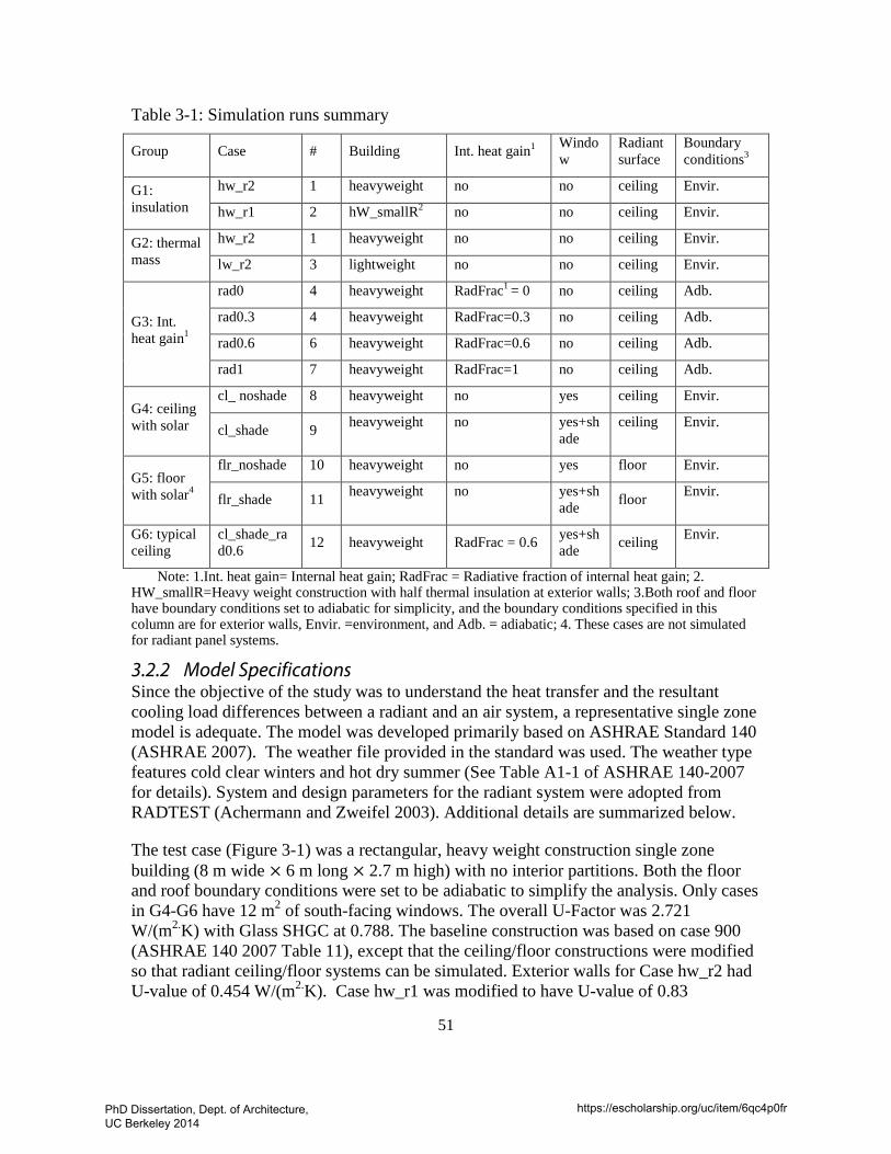
51

Table 3-1: Simulation runs summary

Group Case # Building Int. heat gain1 Window

Radiant surface

Boundary conditions3

G1: insulation

hw_r2 1 heavyweight no no ceiling Envir.

hw_r1 2 hW_smallR2 no no ceiling Envir.

G2: thermal mass

hw_r2 1 heavyweight no no ceiling Envir.

lw_r2 3 lightweight no no ceiling Envir.

G3: Int. heat gain1

rad0 4 heavyweight RadFrac1 = 0 no ceiling Adb.

rad0.3 4 heavyweight RadFrac=0.3 no ceiling Adb.

rad0.6 6 heavyweight RadFrac=0.6 no ceiling Adb.

rad1 7 heavyweight RadFrac=1 no ceiling Adb.

G4: ceiling with solar

cl_ noshade 8 heavyweight no yes ceiling Envir.

cl_shade 9 heavyweight no yes+shade

ceiling Envir.

G5: floor with solar4

flr_noshade 10 heavyweight no yes floor Envir.

flr_shade 11 heavyweight no yes+shade floor Envir.

G6: typical ceiling

cl_shade_rad0.6 12 heavyweight RadFrac = 0.6 yes+sh

ade ceiling Envir.

Note: 1.Int. heat gain= Internal heat gain; RadFrac = Radiative fraction of internal heat gain; 2. HW_smallR=Heavy weight construction with half thermal insulation at exterior walls; 3.Both roof and floor have boundary conditions set to adiabatic for simplicity, and the boundary conditions specified in this column are for exterior walls, Envir. =environment, and Adb. = adiabatic; 4. These cases are not simulated for radiant panel systems.

3.2.2 Model Specifications Since the objective of the study was to understand the heat transfer and the resultant cooling load differences between a radiant and an air system, a representative single zone model is adequate. The model was developed primarily based on ASHRAE Standard 140 (ASHRAE 2007). The weather file provided in the standard was used. The weather type features cold clear winters and hot dry summer (See Table A1-1 of ASHRAE 140-2007 for details). System and design parameters for the radiant system were adopted from RADTEST (Achermann and Zweifel 2003). Additional details are summarized below.

The test case (Figure 3-1) was a rectangular, heavy weight construction single zone building (8 m wide × 6 m long × 2.7 m high) with no interior partitions. Both the floor and roof boundary conditions were set to be adiabatic to simplify the analysis. Only cases in G4-G6 have 12 m2 of south-facing windows. The overall U-Factor was 2.721 W/(m2.K) with Glass SHGC at 0.788. The baseline construction was based on case 900 (ASHRAE 140 2007 Table 11), except that the ceiling/floor constructions were modified so that radiant ceiling/floor systems can be simulated. Exterior walls for Case hw_r2 had U-value of 0.454 W/(m2.K). Case hw_r1 was modified to have U-value of 0.83



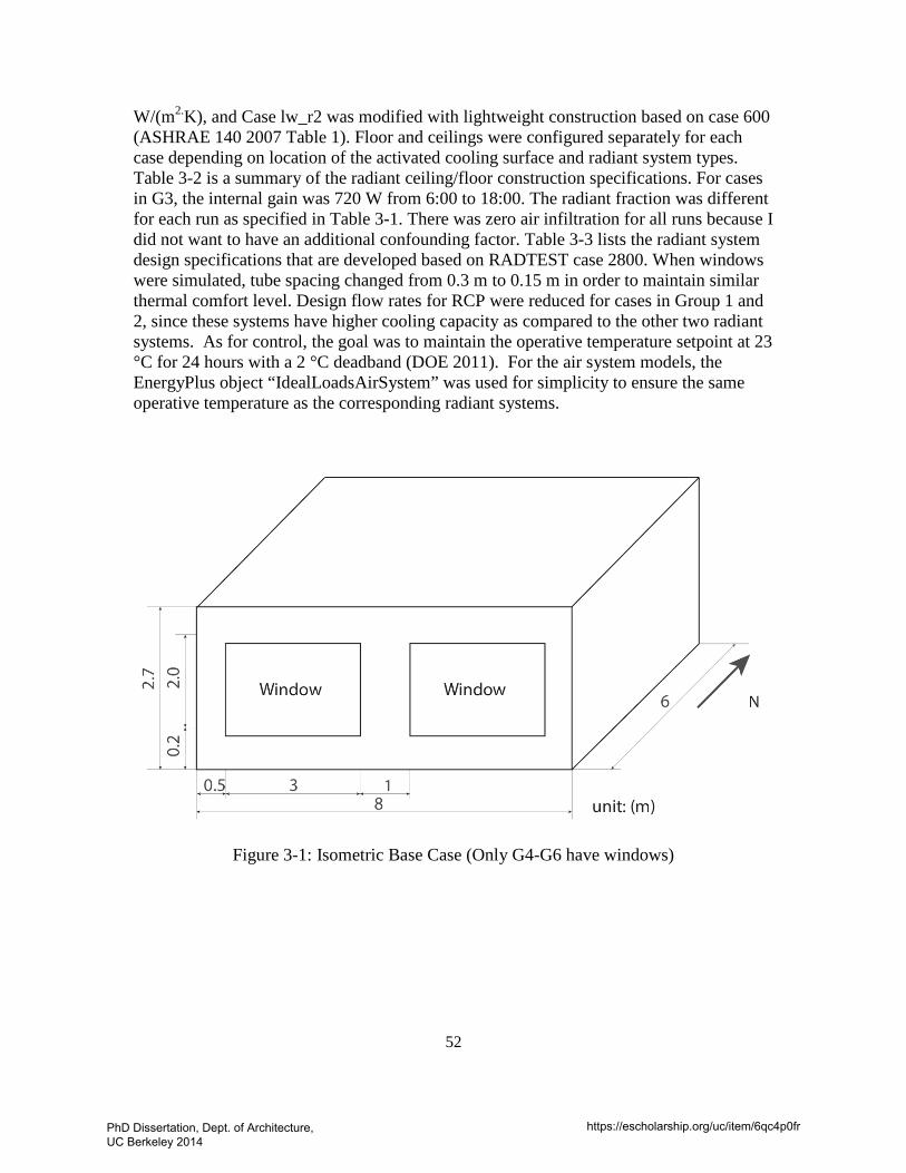
52

W/(m2.K), and Case lw_r2 was modified with lightweight construction based on case 600 (ASHRAE 140 2007 Table 1). Floor and ceilings were configured separately for each case depending on location of the activated cooling surface and radiant system types. Table 3-2 is a summary of the radiant ceiling/floor construction specifications. For cases in G3, the internal gain was 720 W from 6:00 to 18:00. The radiant fraction was different for each run as specified in Table 3-1. There was zero air infiltration for all runs because I did not want to have an additional confounding factor. Table 3-3 lists the radiant system design specifications that are developed based on RADTEST case 2800. When windows were simulated, tube spacing changed from 0.3 m to 0.15 m in order to maintain similar thermal comfort level. Design flow rates for RCP were reduced for cases in Group 1 and 2, since these systems have higher cooling capacity as compared to the other two radiant systems. As for control, the goal was to maintain the operative temperature setpoint at 23 °C for 24 hours with a 2 °C deadband (DOE 2011). For the air system models, the EnergyPlus object “IdealLoadsAirSystem” was used for simplicity to ensure the same operative temperature as the corresponding radiant systems.

Figure 3-1: Isometric Base Case (Only G4-G6 have windows)



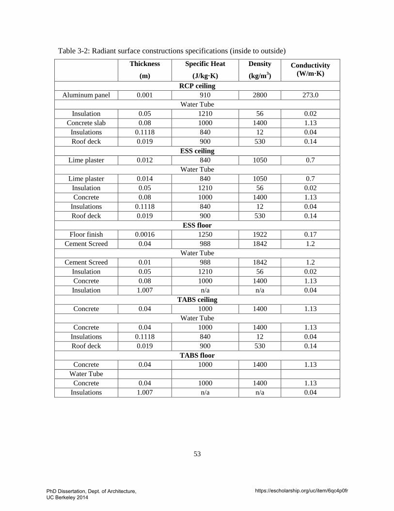
53

Table 3-2: Radiant surface constructions specifications (inside to outside)

Thickness

(m)

Specific Heat

(J/kg·K)

Density

(kg/m3) Conductivity

(W/m·K)

RCP ceiling Aluminum panel 0.001 910 2800 273.0

Water Tube Insulation 0.05 1210 56 0.02

Concrete slab 0.08 1000 1400 1.13 Insulations 0.1118 840 12 0.04 Roof deck 0.019 900 530 0.14

ESS ceiling Lime plaster 0.012 840 1050 0.7

Water Tube Lime plaster 0.014 840 1050 0.7

Insulation 0.05 1210 56 0.02 Concrete 0.08 1000 1400 1.13

Insulations 0.1118 840 12 0.04 Roof deck 0.019 900 530 0.14

ESS floor Floor finish 0.0016 1250 1922 0.17

Cement Screed 0.04 988 1842 1.2 Water Tube

Cement Screed 0.01 988 1842 1.2 Insulation 0.05 1210 56 0.02 Concrete 0.08 1000 1400 1.13 Insulation 1.007 n/a n/a 0.04

TABS ceiling Concrete 0.04 1000 1400 1.13

Water Tube Concrete 0.04 1000 1400 1.13

Insulations 0.1118 840 12 0.04 Roof deck 0.019 900 530 0.14

TABS floor Concrete 0.04 1000 1400 1.13

Water Tube Concrete 0.04 1000 1400 1.13

Insulations 1.007 n/a n/a 0.04



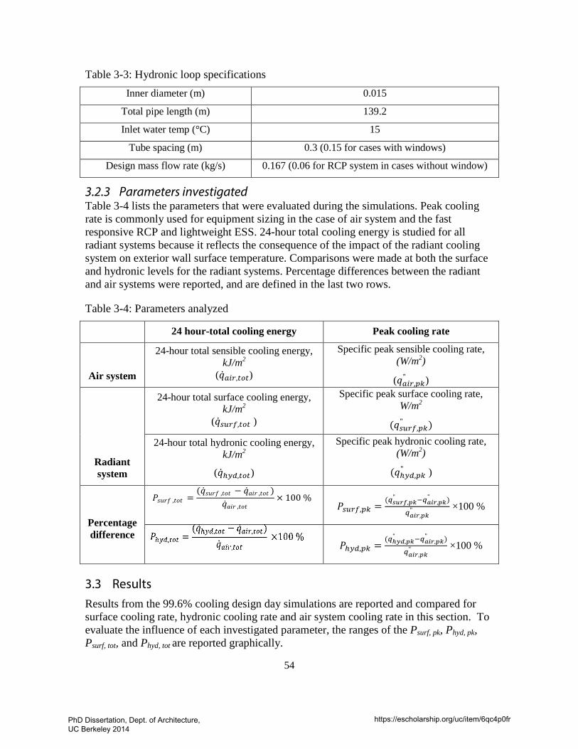
54

Table 3-3: Hydronic loop specifications Inner diameter (m) 0.015

Total pipe length (m) 139.2

Inlet water temp (°C) 15

Tube spacing (m) 0.3 (0.15 for cases with windows)

Design mass flow rate (kg/s) 0.167 (0.06 for RCP system in cases without window)

3.2.3 Parameters investigated Table 3-4 lists the parameters that were evaluated during the simulations. Peak cooling rate is commonly used for equipment sizing in the case of air system and the fast responsive RCP and lightweight ESS. 24-hour total cooling energy is studied for all radiant systems because it reflects the consequence of the impact of the radiant cooling system on exterior wall surface temperature. Comparisons were made at both the surface and hydronic levels for the radiant systems. Percentage differences between the radiant and air systems were reported, and are defined in the last two rows.

Table 3-4: Parameters analyzed

24 hour-total cooling energy Peak cooling rate

Air system

24-hour total sensible cooling energy, kJ/m2

(��𝑞𝑎𝑖𝑟,𝑡𝑜𝑡)

Specific peak sensible cooling rate, (W/m2)

(𝑞𝑞𝑎𝑖𝑟,𝑝𝑘" )

Radiant system

24-hour total surface cooling energy, kJ/m2

(��𝑞𝑠𝑢𝑟𝑓,𝑡𝑜𝑡 )

Specific peak surface cooling rate, W/m2

(𝑞𝑞𝑠𝑢𝑟𝑓,𝑝𝑘" )

24-hour total hydronic cooling energy, kJ/m2

(��𝑞ℎ𝑦𝑑,𝑡𝑜𝑡)

Specific peak hydronic cooling rate, (W/m2)

(𝑞𝑞ℎ𝑦𝑑,𝑝𝑘" )

Percentage difference

𝑃𝑃𝑠𝑠𝑠𝑠𝑠𝑠𝑠𝑠 ,𝑡𝑡𝑡𝑡𝑡𝑡 =(��𝑞𝑠𝑠𝑠𝑠𝑠𝑠𝑠𝑠 ,𝑡𝑡𝑡𝑡𝑡𝑡 − ��𝑞𝑎𝑎𝑎𝑎𝑠𝑠 ,𝑡𝑡𝑡𝑡𝑡𝑡 )

��𝑞𝑎𝑎𝑎𝑎𝑠𝑠 ,𝑡𝑡𝑡𝑡𝑡𝑡× 100 %

𝑃𝑃𝑠𝑢𝑟𝑓,𝑝𝑘 =

(𝑞𝑠𝑢𝑟𝑓,𝑝𝑘" −𝑞𝑎𝑖𝑟,𝑝𝑘

" )

𝑞𝑎𝑖𝑟,𝑝𝑘" ×100 %

𝑃𝑃ℎ𝑦𝑑,𝑝𝑘 =

(𝑞ℎ𝑦𝑑,𝑝𝑘" −𝑞𝑎𝑖𝑟,𝑝𝑘

" )

𝑞𝑎𝑖𝑟,𝑝𝑘" ×100 %

3.3 Results Results from the 99.6% cooling design day simulations are reported and compared for surface cooling rate, hydronic cooling rate and air system cooling rate in this section. To evaluate the influence of each investigated parameter, the ranges of the Psurf, pk, Phyd, pk, Psurf, tot, and Phyd, tot are reported graphically.



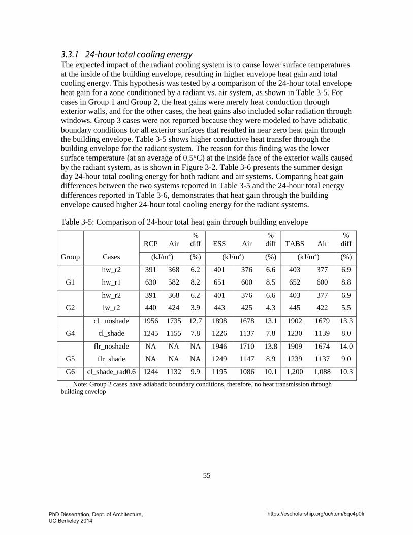
55

3.3.1 24-hour total cooling energy The expected impact of the radiant cooling system is to cause lower surface temperatures at the inside of the building envelope, resulting in higher envelope heat gain and total cooling energy. This hypothesis was tested by a comparison of the 24-hour total envelope heat gain for a zone conditioned by a radiant vs. air system, as shown in Table 3-5. For cases in Group 1 and Group 2, the heat gains were merely heat conduction through exterior walls, and for the other cases, the heat gains also included solar radiation through windows. Group 3 cases were not reported because they were modeled to have adiabatic boundary conditions for all exterior surfaces that resulted in near zero heat gain through the building envelope. Table 3-5 shows higher conductive heat transfer through the building envelope for the radiant system. The reason for this finding was the lower surface temperature (at an average of 0.5°C) at the inside face of the exterior walls caused by the radiant system, as is shown in Figure 3-2. Table 3-6 presents the summer design day 24-hour total cooling energy for both radiant and air systems. Comparing heat gain differences between the two systems reported in Table 3-5 and the 24-hour total energy differences reported in Table 3-6, demonstrates that heat gain through the building envelope caused higher 24-hour total cooling energy for the radiant systems.

Table 3-5: Comparison of 24-hour total heat gain through building envelope

Group Cases

RCP Air %

diff ESS Air %

diff TABS Air %

diff

(kJ/m2) (%) (kJ/m2) (%) (kJ/m2) (%)

G1

hw_r2 391 368 6.2 401 376 6.6 403 377 6.9

hw_r1 630 582 8.2 651 600 8.5 652 600 8.8

G2

hw_r2 391 368 6.2 401 376 6.6 403 377 6.9

lw_r2 440 424 3.9 443 425 4.3 445 422 5.5

G4

cl_ noshade 1956 1735 12.7 1898 1678 13.1 1902 1679 13.3

cl_shade 1245 1155 7.8 1226 1137 7.8 1230 1139 8.0

G5

flr_noshade NA NA NA 1946 1710 13.8 1909 1674 14.0

flr_shade NA NA NA 1249 1147 8.9 1239 1137 9.0

G6 cl_shade_rad0.6 1244 1132 9.9 1195 1086 10.1 1,200 1,088 10.3 Note: Group 2 cases have adiabatic boundary conditions, therefore, no heat transmission through

building envelop



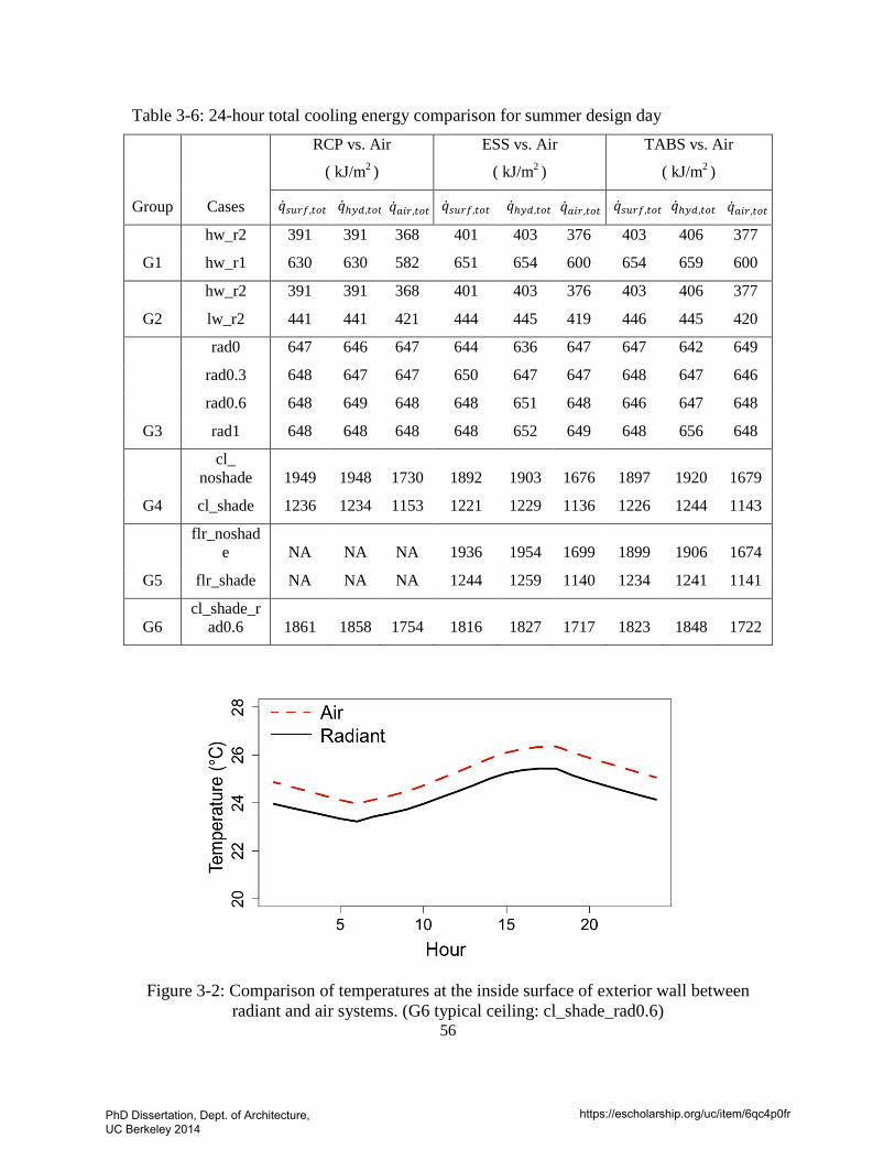
56

Table 3-6: 24-hour total cooling energy comparison for summer design day

Group Cases

RCP vs. Air

( kJ/m2 )

ESS vs. Air

( kJ/m2 )

TABS vs. Air

( kJ/m2 )

��𝑞𝑠𝑢𝑟𝑓,𝑡𝑜𝑡 ��𝑞ℎ𝑦𝑑,𝑡𝑜𝑡 ��𝑞𝑎𝑖𝑟,𝑡𝑜𝑡 ��𝑞𝑠𝑢𝑟𝑓,𝑡𝑜𝑡 ��𝑞ℎ𝑦𝑑,𝑡𝑜𝑡 ��𝑞𝑎𝑖𝑟,𝑡𝑜𝑡 ��𝑞𝑠𝑢𝑟𝑓,𝑡𝑜𝑡 ��𝑞ℎ𝑦𝑑,𝑡𝑜𝑡 ��𝑞𝑎𝑖𝑟,𝑡𝑜𝑡

G1

hw_r2 391 391 368 401 403 376 403 406 377

hw_r1 630 630 582 651 654 600 654 659 600

G2

hw_r2 391 391 368 401 403 376 403 406 377

lw_r2 441 441 421 444 445 419 446 445 420

G3

rad0 647 646 647 644 636 647 647 642 649

rad0.3 648 647 647 650 647 647 648 647 646

rad0.6 648 649 648 648 651 648 646 647 648

rad1 648 648 648 648 652 649 648 656 648

G4

cl_ noshade 1949 1948 1730 1892 1903 1676 1897 1920 1679

cl_shade 1236 1234 1153 1221 1229 1136 1226 1244 1143

G5

flr_noshade NA NA NA 1936 1954 1699 1899 1906 1674

flr_shade NA NA NA 1244 1259 1140 1234 1241 1141

G6 cl_shade_r

ad0.6 1861 1858 1754 1816 1827 1717 1823 1848 1722

Figure 3-2: Comparison of temperatures at the inside surface of exterior wall between

radiant and air systems. (G6 typical ceiling: cl_shade_rad0.6)



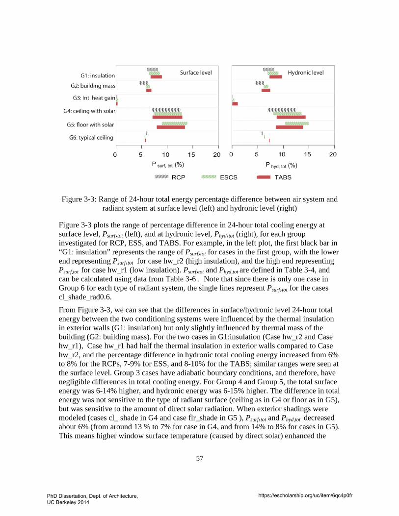
57

Figure 3-3: Range of 24-hour total energy percentage difference between air system and radiant system at surface level (left) and hydronic level (right)

Figure 3-3 plots the range of percentage difference in 24-hour total cooling energy at surface level, Psurf,tot (left), and at hydronic level, Phyd,tot (right), for each group investigated for RCP, ESS, and TABS. For example, in the left plot, the first black bar in “G1: insulation” represents the range of Psurf,tot for cases in the first group, with the lower end representing Psurf,tot for case hw_r2 (high insulation), and the high end representing Psurf,tot for case hw_r1 (low insulation). Psurf,tot and Phyd,tot are defined in Table 3-4, and can be calculated using data from Table 3-6 . Note that since there is only one case in Group 6 for each type of radiant system, the single lines represent Psurf,tot for the cases cl_shade_rad0.6.

From Figure 3-3, we can see that the differences in surface/hydronic level 24-hour total energy between the two conditioning systems were influenced by the thermal insulation in exterior walls (G1: insulation) but only slightly influenced by thermal mass of the building (G2: building mass). For the two cases in G1:insulation (Case hw_r2 and Case hw_r1), Case hw_r1 had half the thermal insulation in exterior walls compared to Case hw_r2, and the percentage difference in hydronic total cooling energy increased from 6% to 8% for the RCPs, 7-9% for ESS, and 8-10% for the TABS; similar ranges were seen at the surface level. Group 3 cases have adiabatic boundary conditions, and therefore, have negligible differences in total cooling energy. For Group 4 and Group 5, the total surface energy was 6-14% higher, and hydronic energy was 6-15% higher. The difference in total energy was not sensitive to the type of radiant surface (ceiling as in G4 or floor as in G5), but was sensitive to the amount of direct solar radiation. When exterior shadings were modeled (cases cl_ shade in G4 and case flr_shade in G5 ), Psurf,tot and Phyd,tot decreased about 6% (from around 13 % to 7% for case in G4, and from 14% to 8% for cases in G5). This means higher window surface temperature (caused by direct solar) enhanced the



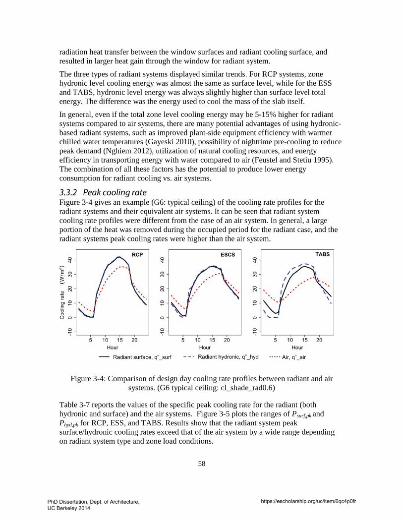
58

radiation heat transfer between the window surfaces and radiant cooling surface, and resulted in larger heat gain through the window for radiant system.

The three types of radiant systems displayed similar trends. For RCP systems, zone hydronic level cooling energy was almost the same as surface level, while for the ESS and TABS, hydronic level energy was always slightly higher than surface level total energy. The difference was the energy used to cool the mass of the slab itself.

In general, even if the total zone level cooling energy may be 5-15% higher for radiant systems compared to air systems, there are many potential advantages of using hydronic-based radiant systems, such as improved plant-side equipment efficiency with warmer chilled water temperatures (Gayeski 2010), possibility of nighttime pre-cooling to reduce peak demand (Nghiem 2012), utilization of natural cooling resources, and energy efficiency in transporting energy with water compared to air (Feustel and Stetiu 1995). The combination of all these factors has the potential to produce lower energy consumption for radiant cooling vs. air systems.

3.3.2 Peak cooling rate Figure 3-4 gives an example (G6: typical ceiling) of the cooling rate profiles for the radiant systems and their equivalent air systems. It can be seen that radiant system cooling rate profiles were different from the case of an air system. In general, a large portion of the heat was removed during the occupied period for the radiant case, and the radiant systems peak cooling rates were higher than the air system.

Figure 3-4: Comparison of design day cooling rate profiles between radiant and air

systems. (G6 typical ceiling: cl_shade_rad0.6)

Table 3-7 reports the values of the specific peak cooling rate for the radiant (both hydronic and surface) and the air systems. Figure 3-5 plots the ranges of Psurf,pk and Phyd,pk for RCP, ESS, and TABS. Results show that the radiant system peak surface/hydronic cooling rates exceed that of the air system by a wide range depending on radiant system type and zone load conditions.



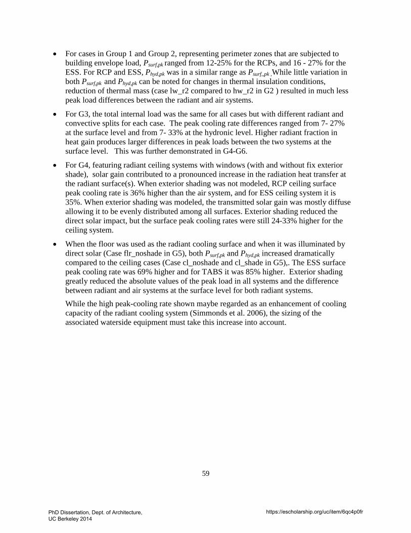
59

• For cases in Group 1 and Group 2, representing perimeter zones that are subjected to building envelope load, Psurf,pk ranged from 12-25% for the RCPs, and 16 - 27% for the ESS. For RCP and ESS, Phyd,pk was in a similar range as Psurf,,pk ,While little variation in both Psurf,pk and Phyd,pk can be noted for changes in thermal insulation conditions, reduction of thermal mass (case lw_r2 compared to hw_r2 in G2 ) resulted in much less peak load differences between the radiant and air systems.

• For G3, the total internal load was the same for all cases but with different radiant and convective splits for each case. The peak cooling rate differences ranged from 7- 27% at the surface level and from 7- 33% at the hydronic level. Higher radiant fraction in heat gain produces larger differences in peak loads between the two systems at the surface level. This was further demonstrated in G4-G6.

• For G4, featuring radiant ceiling systems with windows (with and without fix exterior shade), solar gain contributed to a pronounced increase in the radiation heat transfer at the radiant surface(s). When exterior shading was not modeled, RCP ceiling surface peak cooling rate is 36% higher than the air system, and for ESS ceiling system it is 35%. When exterior shading was modeled, the transmitted solar gain was mostly diffuse allowing it to be evenly distributed among all surfaces. Exterior shading reduced the direct solar impact, but the surface peak cooling rates were still 24-33% higher for the ceiling system.

• When the floor was used as the radiant cooling surface and when it was illuminated by direct solar (Case flr_noshade in G5), both Psurf,pk and Phyd,pk increased dramatically compared to the ceiling cases (Case cl_noshade and cl_shade in G5),. The ESS surface peak cooling rate was 69% higher and for TABS it was 85% higher. Exterior shading greatly reduced the absolute values of the peak load in all systems and the difference between radiant and air systems at the surface level for both radiant systems.

While the high peak-cooling rate shown maybe regarded as an enhancement of cooling capacity of the radiant cooling system (Simmonds et al. 2006), the sizing of the associated waterside equipment must take this increase into account.



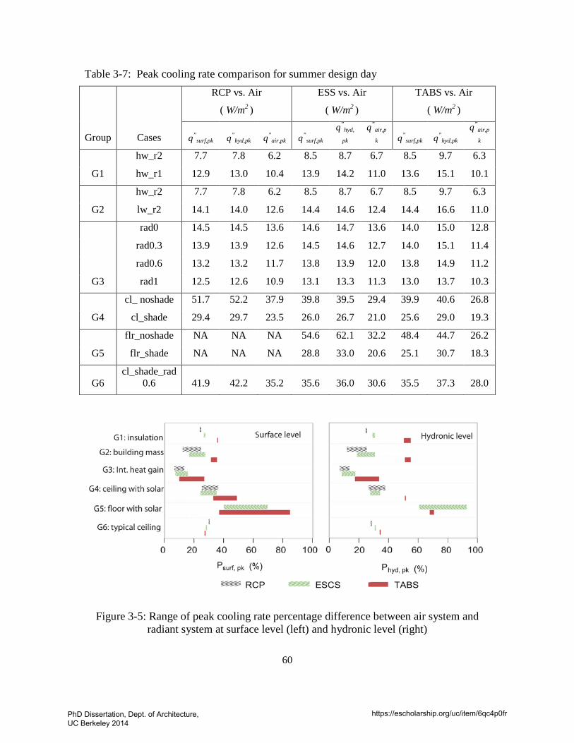
60

Table 3-7: Peak cooling rate comparison for summer design day

Group Cases

RCP vs. Air

( W/m2 )

ESS vs. Air

( W/m2 )

TABS vs. Air

( W/m2 )

q”surf,pk q”

hyd,pk q”air,pk q”

surf,pk q”

hyd,

pk q”

air,p

k q”surf,pk q”

hyd,pk q”

air,p

k

G1

hw_r2 7.7 7.8 6.2 8.5 8.7 6.7 8.5 9.7 6.3

hw_r1 12.9 13.0 10.4 13.9 14.2 11.0 13.6 15.1 10.1

G2

hw_r2 7.7 7.8 6.2 8.5 8.7 6.7 8.5 9.7 6.3

lw_r2 14.1 14.0 12.6 14.4 14.6 12.4 14.4 16.6 11.0

G3

rad0 14.5 14.5 13.6 14.6 14.7 13.6 14.0 15.0 12.8

rad0.3 13.9 13.9 12.6 14.5 14.6 12.7 14.0 15.1 11.4

rad0.6 13.2 13.2 11.7 13.8 13.9 12.0 13.8 14.9 11.2

rad1 12.5 12.6 10.9 13.1 13.3 11.3 13.0 13.7 10.3

G4

cl_ noshade 51.7 52.2 37.9 39.8 39.5 29.4 39.9 40.6 26.8

cl_shade 29.4 29.7 23.5 26.0 26.7 21.0 25.6 29.0 19.3

G5

flr_noshade NA NA NA 54.6 62.1 32.2 48.4 44.7 26.2

flr_shade NA NA NA 28.8 33.0 20.6 25.1 30.7 18.3

G6 cl_shade_rad

0.6 41.9 42.2 35.2 35.6 36.0 30.6 35.5 37.3 28.0

Figure 3-5: Range of peak cooling rate percentage difference between air system and radiant system at surface level (left) and hydronic level (right)



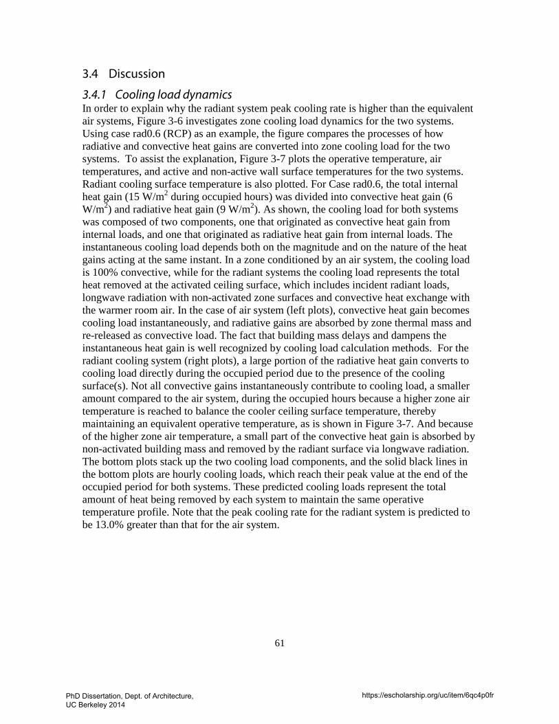
61

3.4 Discussion

3.4.1 Cooling load dynamics In order to explain why the radiant system peak cooling rate is higher than the equivalent air systems, Figure 3-6 investigates zone cooling load dynamics for the two systems. Using case rad0.6 (RCP) as an example, the figure compares the processes of how radiative and convective heat gains are converted into zone cooling load for the two systems. To assist the explanation, Figure 3-7 plots the operative temperature, air temperatures, and active and non-active wall surface temperatures for the two systems. Radiant cooling surface temperature is also plotted. For Case rad0.6, the total internal heat gain (15 W/m2 during occupied hours) was divided into convective heat gain (6 W/m2) and radiative heat gain (9 W/m2). As shown, the cooling load for both systems was composed of two components, one that originated as convective heat gain from internal loads, and one that originated as radiative heat gain from internal loads. The instantaneous cooling load depends both on the magnitude and on the nature of the heat gains acting at the same instant. In a zone conditioned by an air system, the cooling load is 100% convective, while for the radiant systems the cooling load represents the total heat removed at the activated ceiling surface, which includes incident radiant loads, longwave radiation with non-activated zone surfaces and convective heat exchange with the warmer room air. In the case of air system (left plots), convective heat gain becomes cooling load instantaneously, and radiative gains are absorbed by zone thermal mass and re-released as convective load. The fact that building mass delays and dampens the instantaneous heat gain is well recognized by cooling load calculation methods. For the radiant cooling system (right plots), a large portion of the radiative heat gain converts to cooling load directly during the occupied period due to the presence of the cooling surface(s). Not all convective gains instantaneously contribute to cooling load, a smaller amount compared to the air system, during the occupied hours because a higher zone air temperature is reached to balance the cooler ceiling surface temperature, thereby maintaining an equivalent operative temperature, as is shown in Figure 3-7. And because of the higher zone air temperature, a small part of the convective heat gain is absorbed by non-activated building mass and removed by the radiant surface via longwave radiation. The bottom plots stack up the two cooling load components, and the solid black lines in the bottom plots are hourly cooling loads, which reach their peak value at the end of the occupied period for both systems. These predicted cooling loads represent the total amount of heat being removed by each system to maintain the same operative temperature profile. Note that the peak cooling rate for the radiant system is predicted to be 13.0% greater than that for the air system.



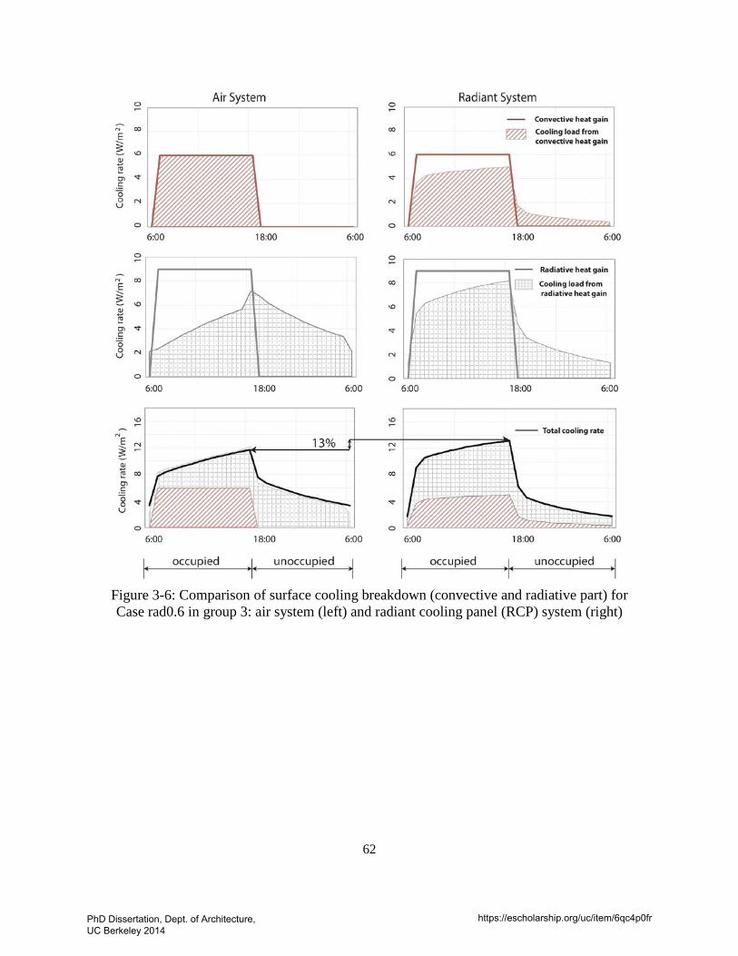
62

Figure 3-6: Comparison of surface cooling breakdown (convective and radiative part) for Case rad0.6 in group 3: air system (left) and radiant cooling panel (RCP) system (right)



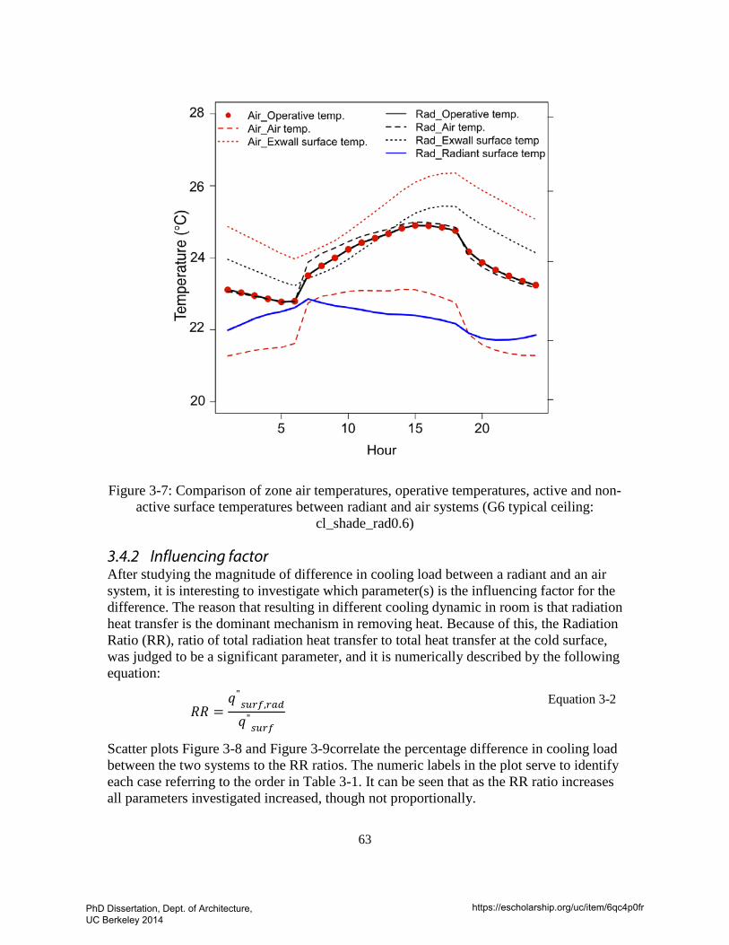
63

Figure 3-7: Comparison of zone air temperatures, operative temperatures, active and non-active surface temperatures between radiant and air systems (G6 typical ceiling:

cl_shade_rad0.6)

3.4.2 Influencing factor After studying the magnitude of difference in cooling load between a radiant and an air system, it is interesting to investigate which parameter(s) is the influencing factor for the difference. The reason that resulting in different cooling dynamic in room is that radiation heat transfer is the dominant mechanism in removing heat. Because of this, the Radiation Ratio (RR), ratio of total radiation heat transfer to total heat transfer at the cold surface, was judged to be a significant parameter, and it is numerically described by the following equation:

𝑅𝑅 =𝑞𝑞"

𝑠𝑢𝑟𝑓,𝑟𝑎𝑑

𝑞𝑞"𝑠𝑢𝑟𝑓

Equation 3-2

Scatter plots Figure 3-8 and Figure 3-9correlate the percentage difference in cooling load between the two systems to the RR ratios. The numeric labels in the plot serve to identify each case referring to the order in Table 3-1. It can be seen that as the RR ratio increases all parameters investigated increased, though not proportionally.



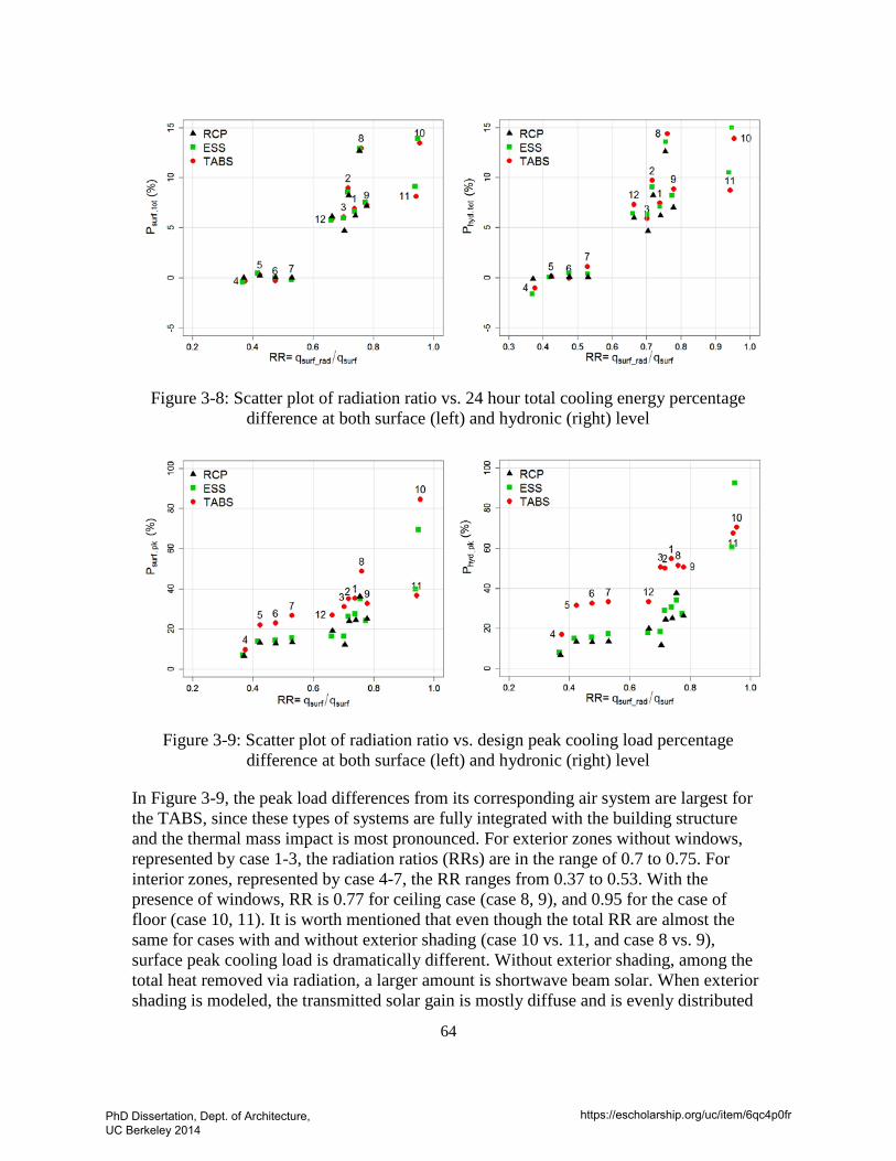
64

Figure 3-8: Scatter plot of radiation ratio vs. 24 hour total cooling energy percentage difference at both surface (left) and hydronic (right) level

Figure 3-9: Scatter plot of radiation ratio vs. design peak cooling load percentage difference at both surface (left) and hydronic (right) level

In Figure 3-9, the peak load differences from its corresponding air system are largest for the TABS, since these types of systems are fully integrated with the building structure and the thermal mass impact is most pronounced. For exterior zones without windows, represented by case 1-3, the radiation ratios (RRs) are in the range of 0.7 to 0.75. For interior zones, represented by case 4-7, the RR ranges from 0.37 to 0.53. With the presence of windows, RR is 0.77 for ceiling case (case 8, 9), and 0.95 for the case of floor (case 10, 11). It is worth mentioned that even though the total RR are almost the same for cases with and without exterior shading (case 10 vs. 11, and case 8 vs. 9), surface peak cooling load is dramatically different. Without exterior shading, among the total heat removed via radiation, a larger amount is shortwave beam solar. When exterior shading is modeled, the transmitted solar gain is mostly diffuse and is evenly distributed



65

among all surfaces, and the majority of the heat is removed by the cooling surface as longwave radiation. This implies that the impact of longwave and shortwave radiation should be considered separately.

When comparing radiant systems and their corresponding air system, the differences in 24-hour total cooling energy does not depend much on the type of radiant system (see Figure 3-8). The distinction in different type of radiation plays an important role, which is similar to the situation discussed for peak cooling load .

3.5 Summary This simulation study investigated the impacts of the presence of an activated cooled surface on zone cooling loads by comparing the peak cooling rate and the 24-hour total cooling energy for radiant and air systems. Three radiant system types (RCP/ESS/TABS) and single zone models were developed for comparison between each radiant system type and their equivalent air system. The models were configured to study the impacts of the following parameters: envelope thermal insulation, thermal mass, type of internal gain, solar heat gain with different shading options, and radiant surface orientation (ceiling, floor). The simulation results are summarized below:

• For the simulated cases, when compared to an air system for equivalent comfort conditions (operative temperature), 24-hour total cooling energy removed by the radiant system as 5-13% higher for the RCP hydronic loop, 6-15% higher for the ESS, and 6-15% higher for the TABS. This was caused by lower surface temperatures at the inside surfaces of the building envelope created by the active (cooled) radiant surface.

• For perimeter zones that were only subjected to building envelope heat gain, Psurf,pk ranged from 12% to 25% for the RCPs, 16% to 27% for the ESS, and 31% to 35% for the TABS. For the RCP and the ESS, Phyd,pk were in the similar range as Psurf,,pk ,but for the TABS, Phyd,pk increased to 50-54%.

• For interior zones with longwave radiant heat gain, the peak cooling rate differences ranged from 7% to 27% at the surface level and from 7% to 33% at the hydronic level. This implies that a higher radiant fraction in heat gain produces larger differences in peak cooling rates between the two systems at the surface level. This was further demonstrated in cases with solar load.

• For perimeter zones and an atrium, where direct solar heat gain constitutes a large portion of the cooling load, the peak cooling load difference is pronounced. When exterior shading was not installed, RCP ceiling surface peak cooling rate is 36% higher than the air system, and it is 35% for ESS ceiling systems, and 49% for TABS ceiling systems. Exterior shading reduced the direct solar impact, but the surface peak cooling rates were still 24-33% higher for the radiant ceiling systems compared to the air system.

• When the floor was used as the radiant cooling surface and when it was illuminated by direct solar, Psurf,,pk and Phyd,,pk increased dramatically compared to the ceiling cases. The ESS surface peak cooling rate was 69% higher and for TABS, 85% higher. Exterior shading greatly reduced the difference between radiant and air



66

systems at the surface level for both radiant systems. However, Phyd,,pk for TABS was not much affected by the installation of shading system.

• Cooling rate differences between the two systems originate from two effects: 1) radiant cooling surface(s) directly remove part of the radiant heat gain and reduce heat accumulation in the building mass; 2) only part of the convective heat gain becomes instantaneous cooling load, the remainder partly contributes to increased air temperature and partly is stored in the building mass and removed by the radiant surface as surface cooling load.

In conclusion, zones conditioned by a radiant system have different peak cooling loads than those conditioned by an air system. While the increase in 24-hour total cooling energy is relatively small and may be offset by other energy savings benefits associated with radiant cooling systems, the differences in peak cooling load both in terms of magnitude and time compared to the air systems require special attention in system and control design.



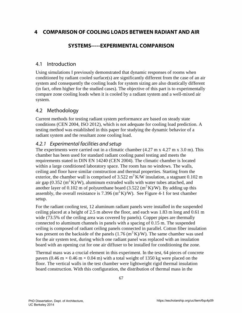
67

4 COMPARISON OF COOLING LOADS BETWEEN RADIANT AND AIR

SYSTEMS-----EXPERIMENTAL COMPARISON

4.1 Introduction Using simulations I previously demonstrated that dynamic responses of rooms when conditioned by radiant cooled surface(s) are significantly different from the case of an air system and consequently the cooling loads for system sizing are also drastically different (in fact, often higher for the studied cases). The objective of this part is to experimentally compare zone cooling loads when it is cooled by a radiant system and a well-mixed air system.

4.2 Methodology Current methods for testing radiant system performance are based on steady state conditions (CEN 2004, ISO 2012), which is not adequate for cooling load prediction. A testing method was established in this paper for studying the dynamic behavior of a radiant system and the resultant zone cooling load.

4.2.1 Experimental facilities and setup The experiments were carried out in a climatic chamber (4.27 m x 4.27 m x 3.0 m). This chamber has been used for standard radiant cooling panel testing and meets the requirements stated in DIN EN 14240 (CEN 2004). The climatic chamber is located within a large conditioned laboratory space. The room has no windows. The walls, ceiling and floor have similar construction and thermal properties. Starting from the exterior, the chamber wall is comprised of 3.522 m2∙K/W insulation, a stagnant 0.102 m air gap (0.352 (m2.K)/W), aluminum extruded walls with water tubes attached, and another layer of 0.102 m of polyurethane board (3.522 (m2.K)/W). By adding up this assembly, the overall resistance is 7.396 (m2.K)/W). See Figure 4-1 for test chamber setup.

For the radiant cooling test, 12 aluminum radiant panels were installed in the suspended ceiling placed at a height of 2.5 m above the floor, and each was 1.83 m long and 0.61 m wide (73.5% of the ceiling area was covered by panels). Copper pipes are thermally connected to aluminum channels in panels with a spacing of 0.15 m. The suspended ceiling is composed of radiant ceiling panels connected in parallel. Cotton fiber insulation was present on the backside of the panels (1.76 (m2.K)/W). The same chamber was used for the air system test, during which one radiant panel was replaced with an insulation board with an opening cut for one air diffuser to be installed for conditioning the zone.

Thermal mass was a crucial element in this experiment. In the test, 64 pieces of concrete pavers (0.46 m × 0.46 m × 0.04 m) with a total weight of 1350 kg were placed on the floor. The vertical walls in the test chamber were lightweight rigid thermal insulation board construction. With this configuration, the distribution of thermal mass in the



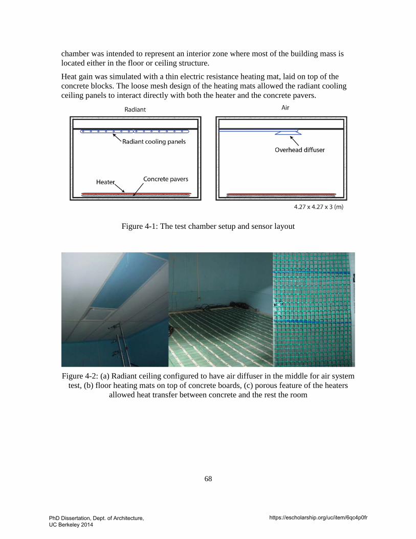
68

chamber was intended to represent an interior zone where most of the building mass is located either in the floor or ceiling structure.

Heat gain was simulated with a thin electric resistance heating mat, laid on top of the concrete blocks. The loose mesh design of the heating mats allowed the radiant cooling ceiling panels to interact directly with both the heater and the concrete pavers.

Figure 4-1: The test chamber setup and sensor layout

Figure 4-2: (a) Radiant ceiling configured to have air diffuser in the middle for air system

test, (b) floor heating mats on top of concrete boards, (c) porous feature of the heaters allowed heat transfer between concrete and the rest the room



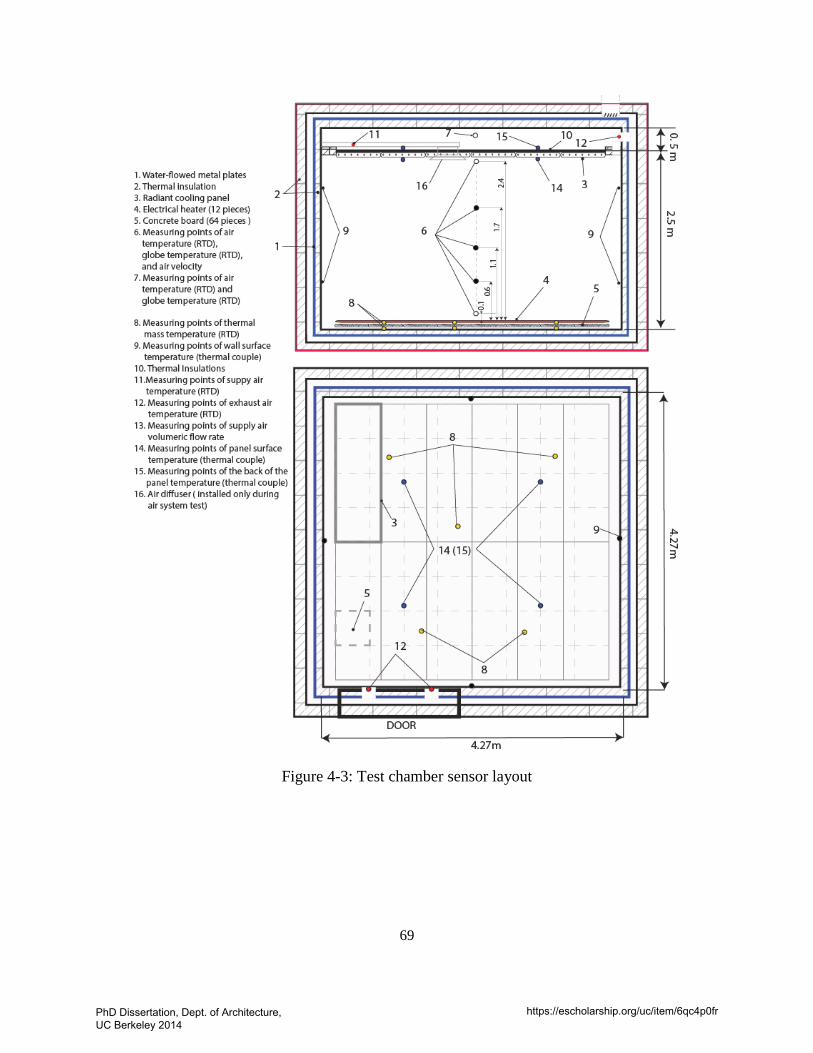
69

Figure 4-3: Test chamber sensor layout



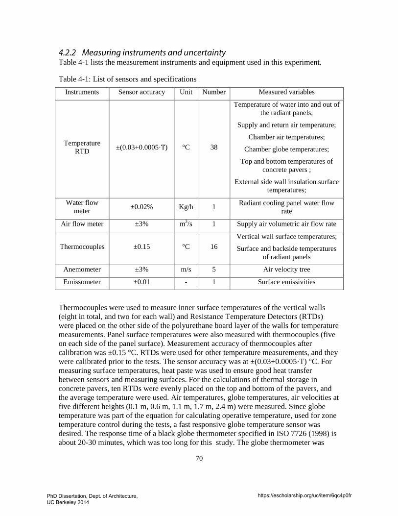
70

4.2.2 Measuring instruments and uncertainty Table 4-1 lists the measurement instruments and equipment used in this experiment.

Table 4-1: List of sensors and specifications Instruments Sensor accuracy Unit Number Measured variables

Temperature RTD ±(0.03+0.0005·T) °C 38

Temperature of water into and out of the radiant panels;

Supply and return air temperature;

Chamber air temperatures;

Chamber globe temperatures;

Top and bottom temperatures of concrete pavers ;

External side wall insulation surface temperatures;

Water flow meter ±0.02% Kg/h 1 Radiant cooling panel water flow

rate

Air flow meter ±3% m3/s 1 Supply air volumetric air flow rate

Thermocouples ±0.15 °C 16 Vertical wall surface temperatures;

Surface and backside temperatures of radiant panels

Anemometer ±3% m/s 5 Air velocity tree

Emissometer ±0.01 - 1 Surface emissivities

Thermocouples were used to measure inner surface temperatures of the vertical walls (eight in total, and two for each wall) and Resistance Temperature Detectors (RTDs) were placed on the other side of the polyurethane board layer of the walls for temperature measurements. Panel surface temperatures were also measured with thermocouples (five on each side of the panel surface). Measurement accuracy of thermocouples after calibration was ±0.15 °C. RTDs were used for other temperature measurements, and they were calibrated prior to the tests. The sensor accuracy was at ±(0.03+0.0005·T) °C. For measuring surface temperatures, heat paste was used to ensure good heat transfer between sensors and measuring surfaces. For the calculations of thermal storage in concrete pavers, ten RTDs were evenly placed on the top and bottom of the pavers, and the average temperature were used. Air temperatures, globe temperatures, air velocities at five different heights (0.1 m, 0.6 m, 1.1 m, 1.7 m, 2.4 m) were measured. Since globe temperature was part of the equation for calculating operative temperature, used for zone temperature control during the tests, a fast responsive globe temperature sensor was desired. The response time of a black globe thermometer specified in ISO 7726 (1998) is about 20-30 minutes, which was too long for this study. The globe thermometer was



71

constructed by inserting an RTD sensor into a table tennis ball coated with gray paint. According to Benton et al. (1990), this type of globe thermometer has a response time of 5.8 minute to reach 90% of its final value, which was considered acceptable for this experiment. Globe temperature and air velocity were used for calculation of mean radiant temperature, and occupied zone operative temperature was calculated as an average of the mean radiant temperatures and air temperatures measured at heights 0.6 m, 1.1 m, and 1.7 m (ISO 1998). Emissivity was measured with an emissometer. Emissivity of internal wall surfaces was 0.20, 0.95 for the concrete floor, and 0.92 for the radiant panels, and uncertainties are ± 0.02. The airflow rate during the air test was measured with a calibrated plate orifice having an accuracy of better than ±3% of the reading. The cooled water mass flow rate was measured with a high quality Coriolis mass flow meter with an accuracy of ±0.02 % of the reading.

4.2.3 Uncertainties analysis The data are analyzed in accordance with the EN ISO 13005 (1993) and JCGM guideline (2008) for the expression of uncertainty. The uncertainty in a primary measurement is estimated as the root sum of the square of the uncertainties due to an independent source. The uncertainty due to an individual source of error can be instrument uncertainty, random error due to spatial variation (when averaging spatial districted sensor), error from data acquisition system, etc. For each type of measure, the global expanded uncertainty was evaluated according to EN ISO 13005 (1993) with a coverage factor at k = 2, i.e. a level of confidence of approximately 95%. Uncertainties in primary measurements are propagated to final calculated variables, which include radiant panel heat extraction rate and airside heat extraction rate.

4.2.4 Uncertainty in airside cooling rate The basic formulation to calculate the air system cooling rate from the space is:

According to Fischer(Fisher 1995), the uncertainties in air properties can be assumed to be negligible, then the uncertainties in the calculated heat extraction rates can be approximated by:

𝑠𝑠𝑞"𝑎 = 𝜌 𝑐𝑝�� 𝑉𝑎.𝑠𝑠∆𝜃𝑎�2

+ � ∆𝑇𝑎.𝑠𝑠𝑉𝑎�2 Equation 4-2

Here, 𝑠𝑠∆𝑇𝑎 = [�𝑠𝑠𝑇𝑎𝑜�2

+ �𝑠𝑠𝑇𝑎𝑖�2

]^0.5. Uncertainty for airflow measurement was estimated to be 6%. The error sources considered for air temperature measurement include sensor accuracy, and spatial variation. Sensor accuracy was listed in Table 4-1. Error due to spatial average was estimated as twice the standard deviation of the measured temperature for 95% confidence (Spitler 1990). Using steady-state data, the return and supply air temperature uncertainties due to spatial variation are estimated to be ±0.11 °C. Uncertainties in primary measurements are propagated to calculate radiant and air system cooling rate uncertainties. For this study, during the periods the heaters were

𝑞𝑞"𝑎 = 𝜌 . 𝑐𝑝.𝑉𝑎.∆𝑇𝑎 Equation 4-1



72

on, the relative uncertainties in air system cooling rate are within ±10% .The level of confidence is 95% (coverage factor 2).

4.2.5 Uncertainty in radiant panel cooling rate Radiant panel cooling rate is the heat extraction rate based on an energy balance on the hydronic circuit. The basic formulation to calculate the radiant system cooling rate is:

𝑞𝑞ℎ𝑦𝑑" = ��𝑐𝑝�𝑤𝑎𝑡𝑒𝑟∆𝑇𝑤 Equation 4-3

The uncertainties in the calculated heat extraction rates can be approximated by:

𝑠𝑠𝑞ℎ𝑦𝑑" = 𝑐𝑤�� 𝑚𝑤.𝑠𝑠∆𝑇𝑤�2

+ � ∆𝑇𝑤.𝑠𝑠𝑚𝑤�2

Equation 4-4

Here, 𝑠𝑠∆𝑇𝑤 = [�𝑠𝑠𝑇𝑤𝑖�2

+ �𝑠𝑠𝑇𝑤𝑜�2

]^0.5. The uncertainty for water flow measurements was ±0.04 %, and uncertainties for measurement accuracy for all water temperatures was twice the sensor accuracy.

For this study, during the periods the heaters were on, the relative uncertainties in radiant system cooling rate uncertainties are within ±8.5 %.

4.2.6 Test procedure For each set of test conditions, two separate experiments were conducted. First, radiant chilled ceiling panels were used to condition the chamber with controlled heat gain. No air system was operated during the radiant system test. Second, an overhead mixing air distribution system was used to remove the same heat gain profile. The 12-hour test procedure was as follows. Prior to beginning the test, the chamber and concrete thermal mass were allowed to reach a uniform, steady state initial temperature of 23 °C. The test was started when the heater was turned on and maintained at a constant value for approximately six hours. The heater was then turned off and the experiment continued for approximately another six hours. For the entire duration of each test, the radiant or air system was controlled to maintain a constant operative temperature in the chamber. Cooling rates were continuously monitored by measuring supply and return temperatures and flow rates for the hydronic radiant panel system and the overhead air distribution system.

Two series of tests were conducted, one at a heat input level of 1080 W (59.3 W/m2), and one at 1500 W (82.4 W/m2). The heater was turned on for 6.1 hours in the 1080 W test, and 6.9 hours in the 1500 W test.

4.3 Results For the radiant system, I calculated the cooling load as the combination of radiant and convective heat exchange at the actively cooled surface during that same time step. I focused on the surface heat transfer because it directly impacts thermal balance and comfort in the zone.

Figure 4-4 shows occupied zone operative temperatures over the course of all experiments. As can be seen, the operative temperature differences between the radiant



73

and air system tests were maintained within ±0.5 °C during all testing periods except for short periods (less than 0.5 hours) immediately after the heaters were turned on or off. Calibrated energy simulation was conducted to check the influence of operative temperature setpoint on resultant system cooling rates. For both radiant and air systems, 0.5°C difference in operative temperature setpoint cause less than 1.5% difference in system cooling rates during the periods when heaters were turned on, and less than 5% after heaters were turned off. Thus, the impacts of the temperature differences between radiant and air system tests can be considered as negligible.

To characterize the dynamic behavior of thermal mass, Figure 4-5 shows the temperatures of concrete and vertical wall surface temperatures. The thick lines are the average of the measurements and the shaded areas represent the variation at different locations. The average temperature of the concrete in the radiant system 1080 W test reaches 28.0 °C at the peak, and 29.0 °C for the air system test. In the 1500 W tests, the peak temperatures were 30.3°C and 31.4°C for the radiant and air system tests, respectively. During the period the heater was on, the surface temperatures of the vertical walls in the chamber during the air system tests were also, on average, 0.7°C (1080 W test) and 1.2 °C (1500 W test) higher compared to radiant system tests. Higher temperatures in the concrete and the chamber structure indicate a greater amount of energy storage when the heater was activated during the air test compared to the radiant test. Given that the same amount of heat is added to the chamber, there is more heat removal by the radiant panels compared to the air system when the heaters are turned on.

Figure 4-4: Comparison of operative temperatures between radiant and air system tests: (A) 1080 W test and (B) 1500 W test



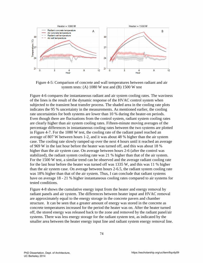
74

Figure 4-5: Comparison of concrete and wall temperatures between radiant and air system tests: (A) 1080 W test and (B) 1500 W test

Figure 4-6 compares the instantaneous radiant and air system cooling rates. The waviness of the lines is the result of the dynamic response of the HVAC control system when subjected to the transient heat transfer process. The shaded area in the cooling rate plots indicates the 95 % uncertainty in the measurements. As mentioned earlier, the cooling rate uncertainties for both systems are lower than 10 % during the heater-on periods. Even though there are fluctuations from the control system, radiant system cooling rates are clearly higher than air system cooling rates. Fifteen-minute moving averages of the percentage differences in instantaneous cooling rates between the two systems are plotted in Figure 4-7. For the 1080 W test, the cooling rate of the radiant panel reached an average of 807 W between hours 1-2, and it was about 48 % higher than the air system case. The cooling rate slowly ramped up over the next 4 hours until it reached an average of 969 W in the last hour before the heater was turned off, and this was about 18 % higher than the air system case. On average between hours 2-6 (after the control was stabilized), the radiant system cooling rate was 21 % higher than that of the air system. For the 1500 W test, a similar trend can be observed and the average radiant cooling rate for the last hour before the heater was turned off was 1335 W, and this was 11 % higher than the air system case. On average between hours 2-6.5, the radiant system cooling rate was 18% higher than that of the air system. Thus, I can conclude that radiant systems have on average 18 - 21 % higher instantaneous cooling rates compared to air systems for tested conditions.

Figure 4-8 shows the cumulative energy input from the heater and energy removal by radiant panels and air system. The differences between heater input and HVAC removal are approximately equal to the energy storage in the concrete pavers and chamber structure. It can be seen that a greater amount of energy was stored in the concrete as concrete temperatures increased for the period the heater was on. After the heater turned off, the stored energy was released back to the zone and removed by the radiant panel/air systems. There was less energy storage for the radiant system test, as indicated by the smaller area between the heater energy input line and radiant system energy removal line.



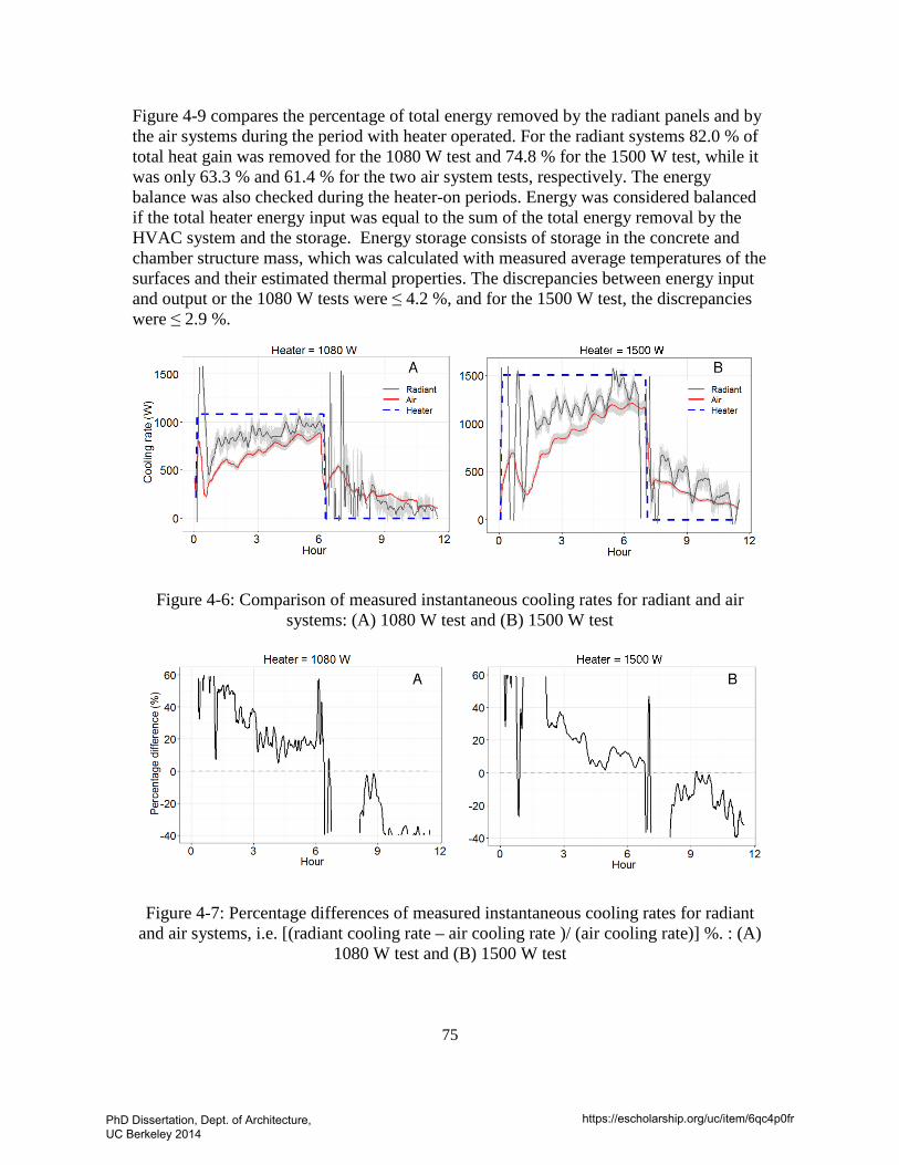
75

Figure 4-9 compares the percentage of total energy removed by the radiant panels and by the air systems during the period with heater operated. For the radiant systems 82.0 % of total heat gain was removed for the 1080 W test and 74.8 % for the 1500 W test, while it was only 63.3 % and 61.4 % for the two air system tests, respectively. The energy balance was also checked during the heater-on periods. Energy was considered balanced if the total heater energy input was equal to the sum of the total energy removal by the HVAC system and the storage. Energy storage consists of storage in the concrete and chamber structure mass, which was calculated with measured average temperatures of the surfaces and their estimated thermal properties. The discrepancies between energy input and output or the 1080 W tests were ≤ 4.2 %, and for the 1500 W test, the discrepancies were ≤ 2.9 %.

Figure 4-6: Comparison of measured instantaneous cooling rates for radiant and air systems: (A) 1080 W test and (B) 1500 W test

Figure 4-7: Percentage differences of measured instantaneous cooling rates for radiant and air systems, i.e. [(radiant cooling rate – air cooling rate )/ (air cooling rate)] %. : (A)

1080 W test and (B) 1500 W test



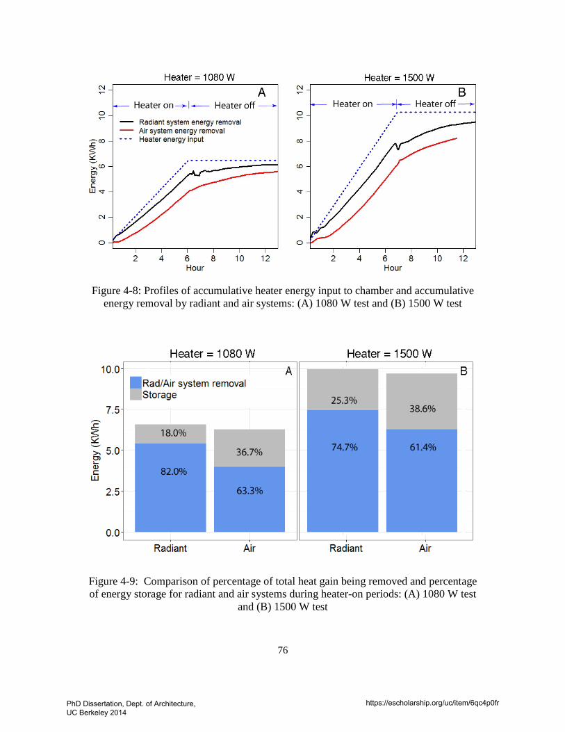
76

Figure 4-8: Profiles of accumulative heater energy input to chamber and accumulative

energy removal by radiant and air systems: (A) 1080 W test and (B) 1500 W test

Figure 4-9: Comparison of percentage of total heat gain being removed and percentage of energy storage for radiant and air systems during heater-on periods: (A) 1080 W test

and (B) 1500 W test



77

4.4 Discussion For the tested conditions, radiant system peak cooling rates were 18 % and 11 % higher for the 1080 W and 1500 W tests, respectively. These numbers agree well with previous simulation results, which showed the differences range from 6-15 % for interior zones depending on radiant ratio of heat source.

It is important to note that for radiant slab systems, cooling rates at the room side (surface level) and at the hydronic level are different due to thermal mass effects. The hydronic level cooling load is a better reference for sizing of cooling plant equipment. A fast responsive radiant panel system was used in the experiment because of their better controllability. The resultant dynamic interactions between the actively cooled surface and its thermal environment and the implications for cooling load differences can well represent the situations with any other types of system that utilize radiation as a heat transfer path to conditioning zone.

TABS or other thermally massive radiant systems are known to respond slowly to control signals. However, as shown in Figure 4-6 to Figure 4-9, the radiant surface is able to respond quickly to changes in heat gains in the zone. Therefore, we may conclude that radiant systems are both quick and slow depending on the context. This feature of radiant system may impact design and operation in many ways. For example, radiant floor systems have wide applications in conditioning areas with high solar load such as atrium and lobbies, because they are considered as especially effective in removing solar load with enhanced cooling capacity reaching 100 W/m2 (Olesen 2008, Zhao et al. 2013). The fast responsive feature is considered as advantageous for maintaining thermal comfort when compared to air systems. On the other hand, designers need to realize that air and radiant system leverage building non-active mass differently. For air systems, heat gain can be significantly delayed becoming cooling load by non-active building mass, and this is beneficial in many applications. For lightweight panel system, which operates during occupied time, thermal delay effect can be weekend. While for the thermally massive radiant systems, cooling requirements may be shift to unoccupied time completely if the radiant layers can be preconditioned. In fact, because these systems are slow to respond to control signals, they are not designed to maintain a constant zone temperature.

Cooling load is not the same as energy consumption. Hydronic-based radiant systems have verified advantages over air systems, such as the improved transport efficiency of using water instead of air as the thermal distribution fluid (Feustel and Stetiu 1995), improved plant side equipment efficiency with warmer cold water temperatures(Gayeski 2010), and, particularly with TABS, the possibility of night pre-cooling using cooling towers (Babiak et al. 2007).

4.5 Summary This experiment demonstrated how the dynamic heat transfer in rooms conditioned by radiant systems is different from those conditioned by air systems. The experimental results confirm that radiant system cooling rates are different from air system rates even when similar thermal comfort level is maintained:



78

• Radiant systems had in average 18 – 21 % higher instantaneous cooling rates than air systems for the tested conditions. This is consistent with the simulated results for cases with internal load with a radiant fraction in the range of 0.6-0.9.

• For the test cases, 75-82 % of total heat gain was removed by the radiant system during the period when the heater was on, while for air system, 61-63 % were removed. The differences were caused by the amount of energy stored in non-active mass. The temperatures of non-active mass (concrete blocks in this paper) are at the peak approximately 1˚C lower for the radiant cases, meaning less energy storage for the radiant cases.

• In the cases of radiant systems, because of the direct coupling between the radiant panel and the thermal mass, there is less heat accumulation and thus the less time lags for heat gain to convert to cooling load.



79

5 COOLING LOAD CALCULATION AND MODELING METHODS FOR

RADIANT SYSTEMS-----APPLICATIONS

5.1 Introduction I have now shown, using both simulation and experiment, that the heat transfer dynamic in rooms conditioned by radiant system is different from air system, and thus the cooling loads are different for the two systems. The objectives of this chapter are to assess the applicability of current cooling load calculation methods when applied to radiant systems, and provide guidance on energy modeling methods. Note that only the ASHRAE heat balance (HB) method and the radiant time series (RTS) method are investigated because they are the two mostly widely adopted standardized methods. To provide recommendations for improvements for those methods, I first review the calculation algorithms in more details. Since both methods involve only the heat transfer process in the space, not through the hydronic slab, the cooling loads I investigated in this chapter are surface cooling loads. Cooling load calculation method for the heavy weight ESS system requires the consideration of control strategies, and is not the focus of the discussion in this chapter.

5.1.1 Heat balance method Cooling load estimation involves calculating a surface-by surface conductive, convective, and radiative heat balance for each room surface and a convective heat balance for the room air. These principles form the foundation for the HB method. The HB method solves the problem directly instead of introducing transformation-based procedures. The advantages are that it contains no arbitrarily set parameters, and no processes are hidden from view. Currently, the HB can be viewed as four distinct processes (see Figure 5-1): 1) Outdoor-side heat balance; 2) Wall conduction process; 3) Indoor-side heat balance; and 4) Air heat balance.

With the assumption that the heat removal mechanism is only by convective cold air, cooling load is calculated to balance the heat transfer in air (the last loop). However, in the case of radiant systems, cooling load is the heat removal by radiant panel surfaces, i.e. cooling load for radiant systems and air systems are different physical variables that are involved in the two heat transfer balance loops. Therefore, directly using the current cooling load calculation procedure based on the HB method is not going to generate the correct cooling load for the radiant system. A definition of cooling load has to be changed to be heat removal at the cooled surface.



80

Figure 5-1: Schematic of the heat balance process in zone (ASHRAE HOF 2013 Chapter

18)

5.1.2 Radiant time series method The RTS method was developed to offer a method that is rigorous, yet does not require iterative calculations, and that quantifies each component’s contribution to the total cooling load. The method is developed to include two time-delay effects inherent in building heat transfer processes: 1) Delay of conductive heat gain through opaque, massive exterior surfaces (walls, roofs, or floors); 2) Delay of radiative heat gain conversion to cooling loads, which as I discussed, is not completely true when an actively cooled surface is used for heat removal.

According to this procedure, each heat gain (conduction portions along with lights, occupants, and equipment) is split into radiative and convective portions. The convective portion is assumed to instantly become cooling load and, therefore, only needs to be summed to find its contribution to the hourly cooling load. The radiative portion, on the other hand, has this time lag and dampening effect. The method for converting the



81

radiative components to cooling loads involves calculations of a series of radiant time factors, which were generated with the assumption of a well-mixed all-air system with no active radiant cooling surface(s) (Spitler et al. 1997).

5.2 Methodology To assess the accuracy of current cooling load calculation methods when applied to radiant systems, I compared the measured results from the experiment described in Chapter 4 with predicted instantaneous cooling rates using the fundamental HB method and simplified RTS method.

A single-zone EnergyPlus (v8.0) model was developed to closely match the test chamber, construction, boundary conditions, and system operating schedule during the experiments. The heater on the floor was modeled using module ZoneHVAC:HighTemperatureRadiant. The default algorithm implemented in EnergyPlus calculates zone cooling load with the ASHRAE recommended procedure, which is the heat convectively removed from the zone air volume to maintain the temperature setpoint. Cooling load for a radiant system is assumed to be the same as for an air system in EnergyPlus. Therefore, the current algorithm does not require modeling of a radiant system to obtain the cooling load, instead an "ideal air system" is recommended to be simulated. However, as mentioned before, this definition cannot directly apply to radiant systems. A new definition of cooling load must be used, which is defined as the combined radiative and convective heat removal rate at the actively cooled surface, instead of heat extraction from the air heat balance, to maintain a temperature setpoint. Therefore, to obtain the actual radiant cooling load, the radiant ceiling panels were modeled. The built-in EnergyPlus radiant model is able to integrate the heat transfer calculation in the systems with changing zone conditions, and therefore is able to capture the system transient behavior (Ghatti 2003, Strand and Baumgartner 2005, DOE 2011). The cooling load for an air system is directly obtained by simulating an ideal air system to maintain 24°C operative temperature. To avoid the complex heat transfer calculations, the RTS method converts heat gain into cooling load by applying periodic response factors (PRF) and conduction time factors (CTF). The CTF and PRFs used to calculate cooling load for the experimental cases were generated by CTF/PRF Generator (Lu), where the climatic chamber geometry and construction specifications were used as inputs. These conversion factors were then used to calculate the resultant cooling load in a spreadsheet where heat gain intensity, schedule and radiant/convective split were specified closely to match testing conditions. Based on calculations of radiation and convective heat transfer at the heated floor, the radiant fraction of heat sources was roughly estimated to be 0.9 for the radiant system and 0.7 for the air system.

5.3 Results Figure 5-2 presents the results for the 1080 W test, similar trends were observed for the 1500 W test. Here, the cooling load for the radiant system was defined as the heat



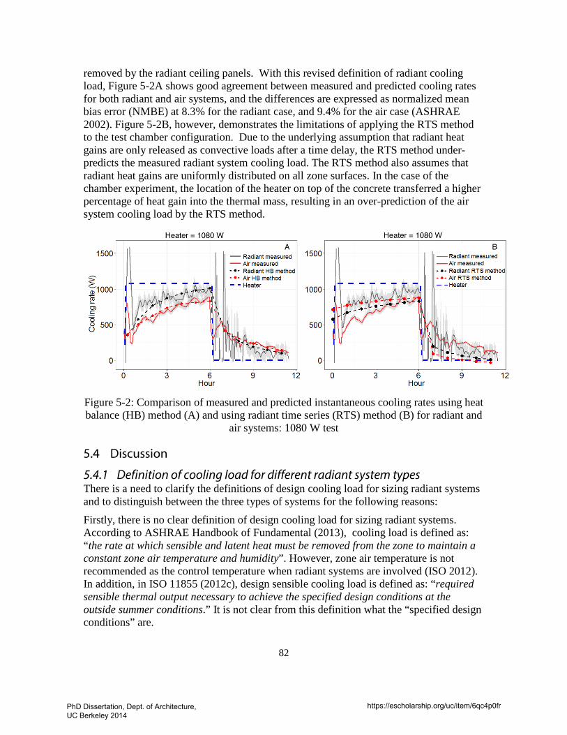
82

removed by the radiant ceiling panels. With this revised definition of radiant cooling load, Figure 5-2A shows good agreement between measured and predicted cooling rates for both radiant and air systems, and the differences are expressed as normalized mean bias error (NMBE) at 8.3% for the radiant case, and 9.4% for the air case (ASHRAE 2002). Figure 5-2B, however, demonstrates the limitations of applying the RTS method to the test chamber configuration. Due to the underlying assumption that radiant heat gains are only released as convective loads after a time delay, the RTS method under-predicts the measured radiant system cooling load. The RTS method also assumes that radiant heat gains are uniformly distributed on all zone surfaces. In the case of the chamber experiment, the location of the heater on top of the concrete transferred a higher percentage of heat gain into the thermal mass, resulting in an over-prediction of the air system cooling load by the RTS method.

Figure 5-2: Comparison of measured and predicted instantaneous cooling rates using heat balance (HB) method (A) and using radiant time series (RTS) method (B) for radiant and

air systems: 1080 W test

5.4 Discussion

5.4.1 Definition of cooling load for different radiant system types There is a need to clarify the definitions of design cooling load for sizing radiant systems and to distinguish between the three types of systems for the following reasons:

Firstly, there is no clear definition of design cooling load for sizing radiant systems. According to ASHRAE Handbook of Fundamental (2013), cooling load is defined as: “the rate at which sensible and latent heat must be removed from the zone to maintain a constant zone air temperature and humidity”. However, zone air temperature is not recommended as the control temperature when radiant systems are involved (ISO 2012). In addition, in ISO 11855 (2012c), design sensible cooling load is defined as: “required sensible thermal output necessary to achieve the specified design conditions at the outside summer conditions.” It is not clear from this definition what the “specified design conditions” are.



83

Secondly, differences in thermal and control characteristics of the three types of radiant system are usually not accounted for when determining design cooling loads. Peak instantaneous cooling load is normally used for sizing air system equipment, but it is not the most relevant for sizing all types of radiant systems. One example is the TABS, as is discussed in Chapter 2.

Thirdly, as mentioned before, radiant cooling systems (ESS and TABS) are integrated with the building mass. As a result, cooling rates at the surface and at the hydronic level are different due to the mass (thermal storage and delay). In cases of air systems, zone cooling load is directly used for sizing the HVAC systems, while in the case of a radiant system, the cooling load imposed on the hydronic loop is a better reference for sizing of cooling plant equipment.

Based on the discussion above, I propose to distinguish the design cooling load definition for sizing the quicker-response RCP/ESS from the slower-response TABS and to define surface cooling load for the determination of required cooling surface area, and to define hydronic cooling load for sizing hydronic equipment (pumps, cooling plant, etc.).

For RCP and lightweight ESS, the proposed cooling load definitions are:

Surface cooling load: the rate at which sensible heat must be removed by the actively cooled surface(s) from the zone to maintain a constant zone operative temperature during the cooling design day. Peak surface cooling load should be used for determining total required cooling surface area.

Hydronic cooling load: the rate at which heat must be removed by the hydronic loop to maintain a constant zone operative temperature during the cooling design day. Peak hydronic cooling load should be used for sizing cooling plant equipment.

The specific surface cooling load can be theoretically calculated by Eq. (2-2) at design conditions. As will be discussed in Chapter 6, the incident radiation is comprised of longwave radiant exchange flux from internal loads, transmitted solar radiation flux absorbed at surface and net shortwave radiation flux to surface from internal loads (lights). During the sizing process, these three terms can be considered as an enhancement of cooling capacity; therefore, even if the peak cooling load of a radiant system may be higher than the cooling load calculated using traditional tools without the capability to capture radiation heat transfer, the total area required may not need to be increased. Future research is needed to quantify how the three incident radiation terms mentioned above will affect sizing of cooling surface area.

For the RCP, hydronic cooling load is the surface cooling load plus heat loss from the backside of the panels, if any. For ESS, the correlation between surface cooling rate and hydronic cooling rate is complicated by the heat conduction through the slab. Part 2 of ISO 11855 (ISO 2012a) recommends two methods for estimating surface cooling output and correlating the output with hydronic side operating conditions.

Design cooling load calculation for TABS has to take into account the control and operation strategy. As discussed in Chapter 2, Part 4 of ISO 11855 (2012b) provides guidance on calculating cooling power demand on the waterside to be used to select the



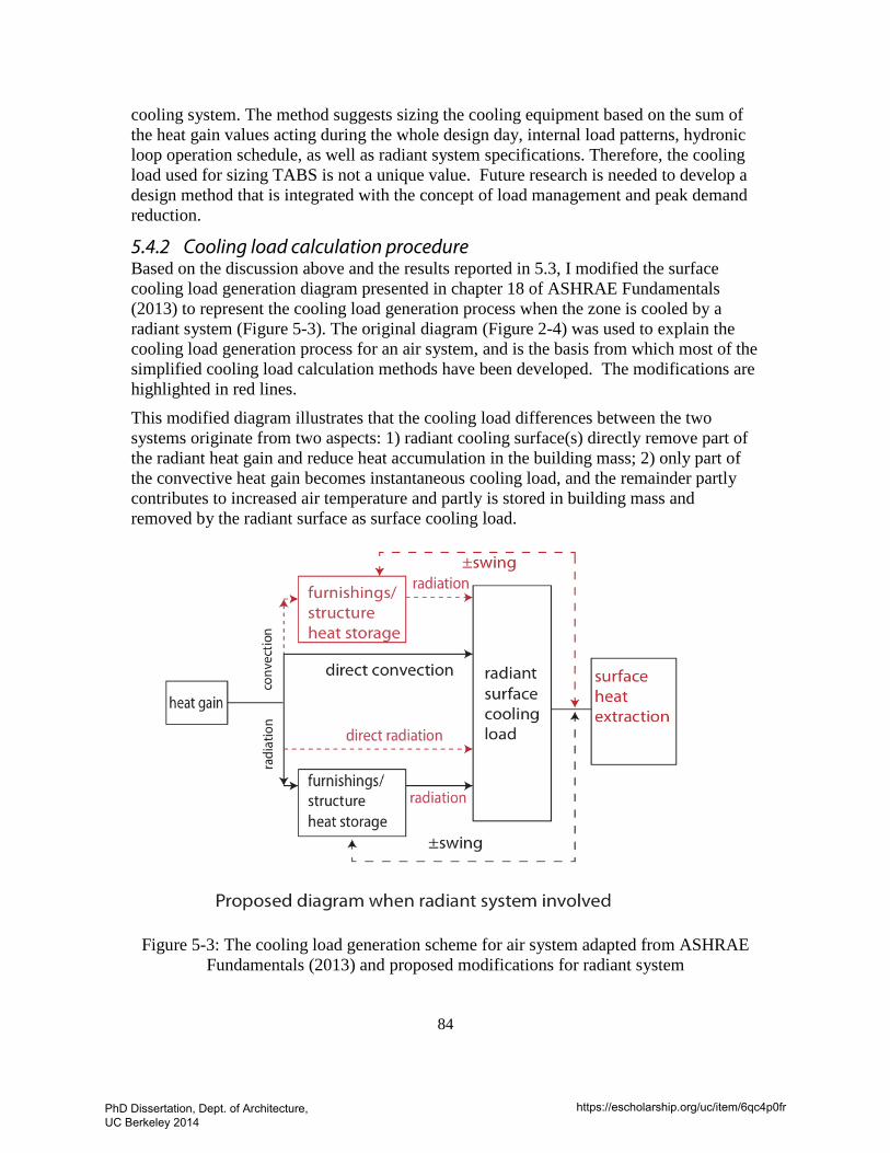
84

cooling system. The method suggests sizing the cooling equipment based on the sum of the heat gain values acting during the whole design day, internal load patterns, hydronic loop operation schedule, as well as radiant system specifications. Therefore, the cooling load used for sizing TABS is not a unique value. Future research is needed to develop a design method that is integrated with the concept of load management and peak demand reduction.

5.4.2 Cooling load calculation procedure Based on the discussion above and the results reported in 5.3, I modified the surface cooling load generation diagram presented in chapter 18 of ASHRAE Fundamentals (2013) to represent the cooling load generation process when the zone is cooled by a radiant system (Figure 5-3). The original diagram (Figure 2-4) was used to explain the cooling load generation process for an air system, and is the basis from which most of the simplified cooling load calculation methods have been developed. The modifications are highlighted in red lines.

This modified diagram illustrates that the cooling load differences between the two systems originate from two aspects: 1) radiant cooling surface(s) directly remove part of the radiant heat gain and reduce heat accumulation in the building mass; 2) only part of the convective heat gain becomes instantaneous cooling load, and the remainder partly contributes to increased air temperature and partly is stored in building mass and removed by the radiant surface as surface cooling load.

Figure 5-3: The cooling load generation scheme for air system adapted from ASHRAE Fundamentals (2013) and proposed modifications for radiant system



85

5.4.3 Impacts on space modeling method As mentioned, current radiant cooling design standards do not explicitly identify the differences in cooling load calculations between radiant and air systems. This results in misapplication of modeling tools in design practice not just for cooling load calculations but also for detailed energy and comfort analysis. Currently, there are three classes of zone thermal models used in energy simulation tools: Heat Balance (HB), Thermal Network (TN), and Transfer Function (TF) models (ASHRAE 2009). The HB and TN methods require relatively extensive computation time and effort from their users, and therefore are not widely adopted in tools used by design practitioners. The tools that use these two zone models, however, have the capability to capture detailed heat transfer processes in the zones and are recommended for use when radiant cooling systems are involved in the design. The weighting factor method, an example of the widely used Transfer Function method, is developed based on similar principle as the RTS method. It converts heat gain into cooling load by applying a series of periodic response factors, which are generated for air system applications. Modifications to the TF method may be possible by generating a new series of response factors that can be applied to cases for radiant systems, but would require future research and is not an easy job due to the coupling of the radiant slab with the building structure.

Radiant systems should be modeled to ensure that the cooled surfaces are participating at the zone level heat transfer during the design calculation. A review of design tools showed that even though dynamic simulation tools are used for energy analysis, the cooling equipment sizing is often based on cooling loads calculated for an ideal air system. For example, I observed this in the EnergyPlus "autosizing" algorithm for radiant systems. In EnergyPlus, the HB method is used as the zone heat transfer model so it has the capability to calculate cooling load accurately when radiant systems are involved. However, it also assumes that the cooling load for a radiant system is the same as for an air system. Therefore, if the "autosizing" function is used, an "ideal air system" is simulated first for load calculation, and this cooling load is used for sizing all associated cooling equipment, including radiant system design mass flow rate, total tube length, and radiant system plant equipment. The users can manually adjust the design parameters if necessary, but failure to realize the cooling load differences between radiant and air systems can produce significant errors.

5.4.4 Proposed improvements in the design standards Based on the discussions, the following text and recommendations could be included in radiant cooling design guidelines to improve understanding of radiant cooling system and to facilitate better design solution:

• The cooling load for zones conditioned by a radiant system is different from the cooling load for zones conditioned by an air system. The differences between the two systems originate from two aspects: 1) Active radiant cooling surface(s) directly remove part of the radiant heat gain and reduce heat accumulation in the building mass; 2) Only part of the convective heat gains becomes instantaneous zone cooling load (as is the case in an air system), and the other portion partly contributes to



86

increased air temperature and partly is stored in building mass and subsequently removed by the active radiant surface as surface cooling load.

• For radiant panels and lightweight embedded systems, peak surface cooling load shall be used for dimensioning total required cooling surface area, and peak hydronic cooling load shall be used for sizing associated cooling equipment. For TABS, equipment sizing depends on total heat gain energy, heat gain pattern, operational strategy, etc.

• Sensible cooling load calculations for radiant systems should utilize dynamic energy simulation programs or design tools based on a fundamental heat balance approach that properly takes into account how heat gains are removed from a zone by an actively cooled surface. Some examples of whole building simulation tools with such capability are EnergyPlus, IES-VE, TRNSYS, IDA-ICE, and ESP-r. I recommend modeling radiant systems utilizing those tools for load prediction and system sizing.

• Simplified cooling load calculation methods, such as RTS or weighting factor method, may lead to incorrect results for radiant systems. These algorithms are implemented in some widely used building thermal simulation or load calculation tools, including HAP (TF), TRANE TRACE (RTS), BLAST, and DOE-2 (TF) based tools such as eQUEST, Energy-pro, Green Building Studio and VisualDOE.

• The following design procedure is recommended for load calculations and system equipment sizing:

1) Conduct a basic cooling load calculation as if an ideal air system with unlimited cooling capacity is used for conditioning the space. This basic cooling load value can be used for comparing different design options. If a radiant system is chosen, the basic cooling load value can be used as a starting point for dimensioning the radiant cooling system;

2) Recalculate design surface cooling load and hydronic cooling load for the radiant system. During this process, the radiant cooling system should be modeled with a computer program that meets the prescribed requirements mentioned above. Size the radiant system properly to satisfy prescribed thermal comfort requirements.

3) Size the cooling plant equipment based on the design hydronic cooling load calculated from step 2.

5.5 Summary There are important limitations in the definition of cooling load for a mixing air system described in Chapter 18 of ASHRAE Handbook of Fundamentals when applied to radiant systems: a) radiant systems remove heat at the cold surface, i.e. the heat transfer balance for load analysis should be conducted at the radiant surface, instead of the air volume, as is in the case for air systems; b) operative temperature, instead of air temperature, is a better reference for calculating the cooling load for radiant system; and c) for radiant panels and lightweight embedded systems, peak surface cooling load shall be used for



87

dimensioning total required cooling surface area, and peak hydronic cooling load shall be used for sizing associated cooling equipment. For thermally massive systems, control strategy should be considered.

Due to the obvious mismatch between how radiant heat transfer is handled in traditional cooling load calculation methods compared to its central role in radiant cooling systems, this dissertation recommends improvements for current cooling load analysis methods and provides guidance for selection of load calculation and modeling tools:

• The current cooling load calculation method based on Heat Balance procedure need to be modified to properly consider the cooling load definition for radiant system.

• Sensible cooling load calculations for radiant systems should utilize dynamic energy simulation programs or design tools based on a fundamental heat balance approach that properly takes into account how heat gains are removed from a zone by an actively cooled surface. Some examples of whole building simulation tools with such capability are EnergyPlus, IES-VE, TRNSYS, IDA-ICE, and ESP-r. I recommend to model radiant system utilizing those tools for load prediction and system sizing.

• Simplified cooling load calculation methods, such as RTS or weighting factor method, may lead to incorrect results for radiant systems. These algorithms are implemented in some widely used building thermal simulation or load calculation tools, including HAP (TF), TRANE TRACE (RTS), BLAST, and DOE-2 (TF) based tools such as eQUEST, Energy-pro, Green Building Studio and VisualDOE.

• The above recommendations also directly apply to the selection of whole building energy simulation software for evaluation of system energy and thermal comfort performance.



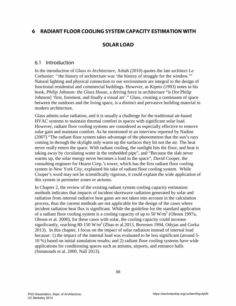
88

6 RADIANT FLOOR COOLING SYSTEM CAPACITY ESTIMATION WITH

SOLAR LOAD

6.1 Introduction In the introduction of Glass in Architecture, Arbab (2010) quotes the late architect Le Corbusier: ‘‘the history of architecture was ‘the history of struggle for the window.’” Natural lighting and physical connection to our environment are integral to the design of functional residential and commercial buildings. However, as Kipnis (1993) notes in his book, Philip Johnson: the Glass House, a driving force in architecture “is [for Philip Johnson] ‘first, foremost, and finally a visual art’.” Glass, creating a continuum of space between the outdoors and the living space, is a distinct and pervasive building material in modern architecture.

Glass admits solar radiation, and it is usually a challenge for the traditional air-based HVAC systems to maintain thermal comfort in spaces with significant solar load. However, radiant floor cooling systems are considered as especially effective to remove solar gain and maintain comfort. As he mentioned in an interview reported by Nadine (2007) “The radiant floor system takes advantage of the phenomenon that the sun’s rays coming in through the skylight only warm up the surfaces they hit not the air. The heat never really enters the space. With radiant cooling, the sunlight hits the floor, and heat is taking away by circulating water in the embedded pipe”, and “Because the slab never warms up, the solar energy never becomes a load in the space”, David Cooper, the consulting engineer for Hearst Corp.’s tower, which has the first radiant floor cooling system in New York City, explained his take of radiant floor cooling system. While Cooper’s word may not be scientifically rigorous, it could explain the wide application of this system in perimeter zones or atriums.

In Chapter 2, the review of the existing radiant system cooling capacity estimation methods indicates that impacts of incident shortwave radiation generated by solar and radiation from internal radiative heat gains are not taken into account in the calculation process, thus the current methods are not applicable for the design of the cases where incident radiation heat flux is significant. While the guideline for the standard application of a radiant floor cooling system is a cooling capacity of up to 50 W/m2 (Olesen 1997a, Olesen et al. 2000), for these cases with solar, the cooling capacity could increase significantly, reaching 80-150 W/m2 (Zhao et al.2013, Borresen 1994, Odyjas and Gorka 2013). In this chapter, I focus on the impact of solar radiation instead of internal load because: 1) the impact of the internal load was evaluated to be less significant (around 5-10 %) based on initial simulation results; and 2) radiant floor cooling systems have wide applications for conditioning spaces such as atriums, airports, and entrance halls (Simmonds et al. 2000, Nall 2013).



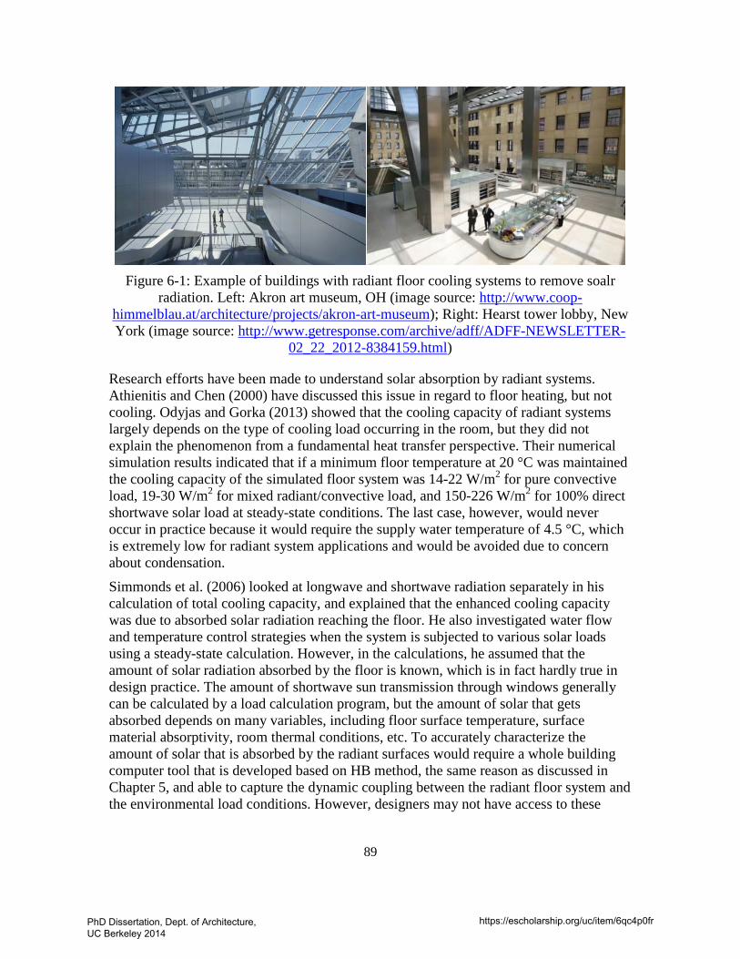
89

Figure 6-1: Example of buildings with radiant floor cooling systems to remove soalr

radiation. Left: Akron art museum, OH (image source: http://www.coop-himmelblau.at/architecture/projects/akron-art-museum); Right: Hearst tower lobby, New York (image source: http://www.getresponse.com/archive/adff/ADFF-NEWSLETTER-

02_22_2012-8384159.html)

Research efforts have been made to understand solar absorption by radiant systems. Athienitis and Chen (2000) have discussed this issue in regard to floor heating, but not cooling. Odyjas and Gorka (2013) showed that the cooling capacity of radiant systems largely depends on the type of cooling load occurring in the room, but they did not explain the phenomenon from a fundamental heat transfer perspective. Their numerical simulation results indicated that if a minimum floor temperature at 20 °C was maintained the cooling capacity of the simulated floor system was 14-22 W/m2 for pure convective load, 19-30 W/m2 for mixed radiant/convective load, and 150-226 W/m2 for 100% direct shortwave solar load at steady-state conditions. The last case, however, would never occur in practice because it would require the supply water temperature of 4.5 °C, which is extremely low for radiant system applications and would be avoided due to concern about condensation.

Simmonds et al. (2006) looked at longwave and shortwave radiation separately in his calculation of total cooling capacity, and explained that the enhanced cooling capacity was due to absorbed solar radiation reaching the floor. He also investigated water flow and temperature control strategies when the system is subjected to various solar loads using a steady-state calculation. However, in the calculations, he assumed that the amount of solar radiation absorbed by the floor is known, which is in fact hardly true in design practice. The amount of shortwave sun transmission through windows generally can be calculated by a load calculation program, but the amount of solar that gets absorbed depends on many variables, including floor surface temperature, surface material absorptivity, room thermal conditions, etc. To accurately characterize the amount of solar that is absorbed by the radiant surfaces would require a whole building computer tool that is developed based on HB method, the same reason as discussed in Chapter 5, and able to capture the dynamic coupling between the radiant floor system and the environmental load conditions. However, designers may not have access to these



http://www.coop-himmelblau.at/architecture/projects/akron-art-museum

http://www.coop-himmelblau.at/architecture/projects/akron-art-museum

http://www.getresponse.com/archive/adff/ADFF-NEWSLETTER-02_22_2012-8384159.html

http://www.getresponse.com/archive/adff/ADFF-NEWSLETTER-02_22_2012-8384159.html

90

tools or may be constraint by the time for analysis at such detailed level. Thus, a simplified method for predicting the amount of absorbed solar is desirable.

Causone (2010) used a lighting simulation tool to quantify the ratio of the amount of solar that is directly absorbed by radiant ceilings to the total solar heat gain to the space. He studied cases with different aspect ratios, window orientations, surface material absorptivity, and locations. However, besides the fact that his study was focused on radiant ceiling applications, there are limitations in his method: 1) the lighting tool can only figure out the “solar patches”, and the influence of the cooled surfaces was not considered; and 2) the calculations were steady-state analysis. At one point, the authors proposed that a fictitious heat transfer coefficient could be introduced to characterize the improvement of heat transfer due to solar radiation. The heat transfer coefficient could be a function of directly absorbed solar and the temperature difference between floor surface and the room operative temperature. However, they did not provide an explicit expression for characterizing this heat transfer coefficient.

For designers, being able to accurately predict radiant system cooling capacity is critical not just for the design of the radiant system but also for its associated air system. As radiant systems provide only sensible cooling, they are typically configured as a hybrid with an air system, which is used for ventilation, dehumidification and supplemental cooling if needed. The desired capacity of the air system is directly related to the radiant system cooling capacity and the underestimation of radiant system capacity can lead to oversizing the air system.

In summary, the goals of the study presented in this chapter are to: 1) use dynamic simulation tools to investigate the impact of solar radiation on floor cooling capacity for different design scenarios; and 2) develop a simplified method to calculate radiant floor cooling capacity and sizing of the associated air systems when direct solar radiation is present.

6.2 Solar radiation in buildings

6.2.1 Modeling of solar radiation in buildings To evaluate its impact on design and control, it is critical to have a good estimation of the amount of incident solar on the radiant surface and, ultimately, the actual amount of solar absorbed by a radiant cooling surface.

Solar radiation is a particular kind of thermal radiation, which is basically an electromagnetic field. Any discussion and analysis involving solar radiation is bound to be complicated. While most thermal radiation analysis is greatly simplified when building surface may be treated as grey (surfaces with radiation properties independent of wavelength) and diffuse (surfaces with radiation properties independent of direction), it is an exception when dealing with solar radiation. Solar radiation is full spectral light, but it is treated as shortwave for the following reasons: a) as suggested by the Wien’s displacement law, solar radiation peaks at about 500nm, b) after the screening due to dust and pollutants in the atmosphere, which is particularly concentrated in the infrared spectral region (750nm-4000nm), most solar radiation that reaches the surface of the



91

earth is in shortwave length (Howell et al. 2011). In addition, because most building interior materials have relatively small shortwave absorbance (for example, light color plaster may have shortwave absorptance of 0.3-0.5 and a longwave absorptance of 0.85-0.95(Kuehn et al. 1998, Howell et al. 2011)), a significant portion of incident solar is reflected back to the space or the outdoor environment, and distribution of solar radiation inside the space become important. In order to simplify the analysis, I will: 1) focus the discussion on conditions after solar radiation has been transmitted through the window, 2) base the analysis on the so-called “two-band” model (Spitler 2011). This means, in heat transfer analysis, surfaces including the radiant cooling surfaces have only two absorptance, one for shortwave and one for longwave. This is valid based on the fact that thermal radiation wavelength distributions prevalent in buildings maybe approximately lumped into two categories, short- and long-wave radiation. The long wavelength radiation includes all radiations emitted at low temperatures compared to the sun. The short wavelength sources include radiation emitted by lighting and solar radiation.

The transmitted solar through the window can be categorized into two parts, diffuse solar and direct solar. Estimation of the amount of incident solar onto a radiant cooling surface requires an estimate of how the transmitted direct and diffuse solar radiations are distributed. In other words, the amount of transmitted solar radiation absorbed by each surface in the room, including the radiant cooling surfaces must be determined. This can be (and sometimes is) analyzed in a very detailed manner, accounting for exactly where the radiation strikes each room surface, and then accounting for each reflection until it is all absorbed. For example, EnergyPlus use a ray-tracing method for this analysis. The program calculates the amount of beam radiation falling on each surface in the zone, including floor, walls and windows, by projecting the sun's rays through the exterior windows, taking into account the effect of exterior shadowing surfaces (e.g. adjacent buildings) and window shading devices.

In summary, incident solar radiation on radiant surfaces is affected by many parameters, including total transmitted solar (beam and diffuse solar), distribution of solar in the space, zone geometry, radiant surface location, cooling surface radiation properties, etc.

6.2.2 Radiant cooling surface thermal response Radiant floor cooling is considered especially effective in maintaining thermal comfort in spaces exposed to solar heat gain. In an all-air system, when solar radiation hits the building surfaces, it first warms up the surfaces, and as heat accumulates in the mass, the operative temperature in the space increases and may result in thermal discomfort. To remove this heat, a large amount of cool air has to be supplied to the space, but it can be removed only with a time delay when it is released back to air by convection heat transfer. Therefore, for the all-air system, solar heat gain converts to cooling load at a later time and is dampened. This phenomenon is the thermal delay effect. For a radiant floor cooling system, especially for a system that operates continuously or intermittently with a short interval, solar heat gain incident on the floor will be removed immediately by cold water that circulates in the slab, such that the operative temperature in the space can be well maintained. While this can be considered as beneficial for maintaining thermal comfort, it can be also considered as an increase of cooling load for the radiant cooling



92

slab and the primary system (chiller/cooling tower/pumps), as has been extensively discussed in Chapter 3-5. Therefore, even though the actual cooling capacity of a radiant floor could be higher than the standard recommended values when it is illuminated by either direct or diffuse solar, in general, a successful radiant system design will minimize the solar heat gain to the building. However, for cases such as atria, airports, and perimeter areas when solar radiation is desirable, the impact of solar should be properly considered to achieve optimal sizing of radiant floor cooling systems. This is particularly important because the sizing of their associated air system also depends on an accurate prediction of floor capacity. I will discuss these issues in more detail in the following sections.

6.3 Impact of solar heat gain on radiant floor cooling capacity

6.3.1 Standardized cooling capacity methods As mentioned in Chapter 2, there are two standardized ways to represent system capacity. The first one directly correlates surface heat flux (cooling capacity) to the temperature differences between room operative temperature and radiant surface(s), and the second approach represents system capacity with a lumped thermal resistance and a mean temperature difference between the cooling medium and the space. Here, I will first investigate the heat transfer process at the surface, and this allows me to explicitly pinpoint which heat transfer component might be missing in the calculation process. However, since most manufacturers report radiant system capacity using the second approach, I will also report the system capacity in this format, which is expressed as:

𝑞𝑞" = 𝐾 ∙ ∆𝑇ℎ𝑛 Equation 6-1

Where, n is a constant, and equal to 1 for the embedded systems according to ISO 11855. Both K and n are to be determined.

For the radiant floor cooling system that we studied in this paper, K can be calculated using the following steps. First, calculate the K H, floor for floor heating systems using the correlations for system type A-D (see Chapter 1 for definition).

K H, floor = B ( ∏i αi,m ) Equation 6-2

Here, B is a system dependent coefficient, ∏i αi,m is the power product linking the parameters that can be calculated with the information of the floor construction using methods documented in Appendix A of ISO 11855 part 2. To obtain K for floor cooling system, a conversion has to be conducted:

𝐾 = 𝐾𝐻�∆𝑅𝛼,,𝑅𝜆,𝐵� =𝐾𝐻,𝑓𝑙𝑜𝑜𝑟

1 +∆𝑅𝛼, + 𝑅𝜆,𝐵

𝑅𝜆,𝐵�𝐾𝐻,𝑓𝑙𝑜𝑜𝑟𝐾∗

𝐻,𝑓𝑙𝑜𝑜𝑟− 1�

Equation 6-3



93

Here, ∆Rα = 1/α -1/10.8, and α is the total heat transfer coefficient depending on surface type (floor/celling/wall) and application (heating/cooling), Rλ,B is the thermal resistance of surface covering, K*

H, floor is the resistance when Rλ,B = 0.15.

Definition of ∆𝑇ℎ depends on system types and applications, and for embedded floor system, ∆𝑇ℎ can be calculated as:

∆𝑇ℎ =(𝑇𝑤𝑖 − 𝑇𝑤𝑜)

𝑙𝑛 [ (𝑇𝑤𝑖 – 𝑇𝑜𝑝𝑡)/ (𝑇𝑤𝑜 – 𝑇𝑜𝑝𝑡 )]

Equation 6-4

Where, 𝑇𝑤𝑖, and 𝑇𝑤𝑜is the supply and return water temperature respectively, °C, and 𝑇𝑜𝑝𝑡 is the room operative temperature, °C.

6.3.2 Methodology To verify and quantify the impacts of solar on radiant system capacity, and ultimately provide an improved method for sizing of the radiant and associated air system, I adopted the following methodology:

• Use Energy Plus v7.2 to model a single zone with windows to be conditioned by a radiant floor system. A full matrix of simulation runs was conducted to cover a wide range of design options.

• Investigate the heat transfer process at the radiant surface to numerically understand the reasons for the limitations in the current calculation approaches. Then use the simulated radiant system cooling capacity to compare to the cooling capacity calculated using the ISO method, to further gauge the applicability of the ISO method.

• Develop a new simplified method that can be used for predicting the radiant system capacity when there is solar load.

• Investigate the implications for sizing of the associated air systems with enhanced radiant floor capacity.

• Demonstrate how the designers could use the new method to obtain a better solution for air system size.

6.3.2.1 Modeling approach EnergyPlus v7.2 was used for the study. Detailed solar simulation algorithm employed in EnergyPlus can be found in its Engineering Reference, and basically a “ray tracing” method is used to track the paths of the beam and diffuse solar coming through the fenestration systems. The heat balance algorithms can adequately capture the dynamics of the absorbed solar load and the operating conditions of the cold floors.

The single zone model used for this study was developed based on ASHRAE Standard 140 (ASHRAE 2007). Only a radiant system was modelled when the investigation was focused on the fundamentals. Radiant system design parameters were based on RADTEST (Achermann and Zweifel 2003). The parameters and their variations investigated include: shortwave absorptivity of floor surface material (0.4/0.8), shading options (Interior blinds/No shading), window-to-wall ratio (40/55/70/95), topping thickness of radiant slab system (5/7/10 cm), zone orientation (east/west/south), building



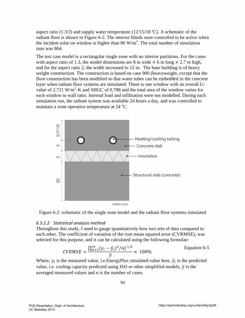
94

aspect ratio (1.3/2) and supply water temperature (12/15/18 °C). A schematic of the radiant floor is shown in Figure 6-2. The interior blinds were controlled to be active when the incident solar on window is higher than 80 W/m2. The total number of simulation runs was 864.

The test case model is a rectangular single zone with no interior partitions. For the cases with aspect ratio of 1.3, the model dimensions are 8 m wide × 6 m long × 2.7 m high, and for the aspect ratio 2, the width increased to 12 m. The base building is of heavy weight construction. The construction is based on case 900 (heavyweight, except that the floor construction has been modified so that water tubes can be embedded in the concrete layer when radiant floor systems are simulated. There is one window with an overall U-value of 2.721 W/m2·K and SHGC of 0.788 and the total area of the window varies for each window to wall ratio. Internal load and infiltration were not modelled. During each simulation run, the radiant system was available 24 hours a day, and was controlled to maintain a zone operative temperature at 24 °C.

Figure 6-2: schematic of the single zone model and the radiant floor systems simulated

6.3.2.2 Statistical analysis method Throughout this study, I need to gauge quantitatively how two sets of data compared to each other. The coefficient of variation of the root mean squared error (CVRMSE), was selected for this purpose, and it can be calculated using the following formulae:

𝐶𝑉𝑅𝑀𝑆𝐸 =[∑ (𝑦𝑖 − 𝑦�𝑖)2𝑛

𝑖=1 𝑛⁄ ] 1/2

𝑦�× 100%

Equation 6-5

Where, 𝑦𝑖 is the measured value, i.e.EnergyPlus simulated value here, 𝑦�𝑖 is the predicted value, i.e. cooling capacity predicted using ISO or other simplified models, 𝑦� is the averaged measured values and n is the number of cases.



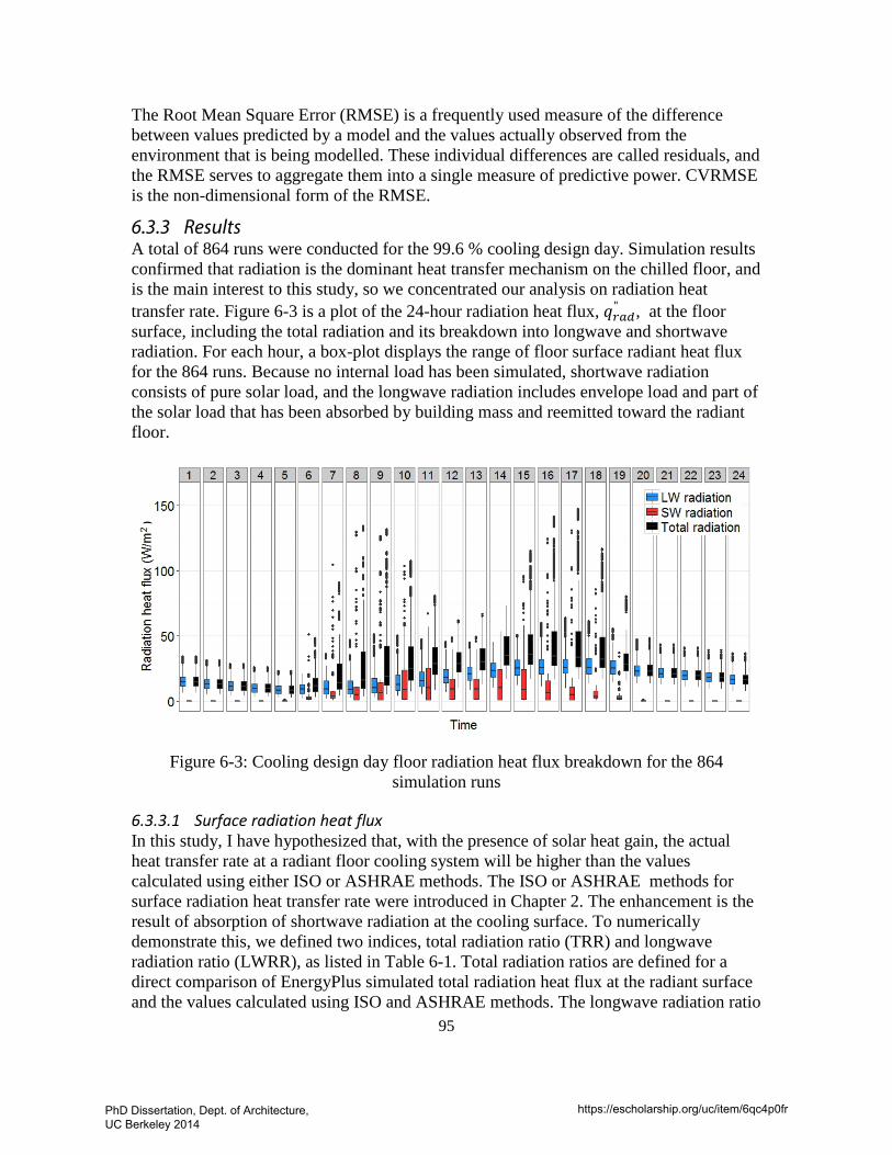
95

The Root Mean Square Error (RMSE) is a frequently used measure of the difference between values predicted by a model and the values actually observed from the environment that is being modelled. These individual differences are called residuals, and the RMSE serves to aggregate them into a single measure of predictive power. CVRMSE is the non-dimensional form of the RMSE.

6.3.3 Results A total of 864 runs were conducted for the 99.6 % cooling design day. Simulation results confirmed that radiation is the dominant heat transfer mechanism on the chilled floor, and is the main interest to this study, so we concentrated our analysis on radiation heat transfer rate. Figure 6-3 is a plot of the 24-hour radiation heat flux, 𝑞𝑞𝑟𝑎𝑑" , at the floor surface, including the total radiation and its breakdown into longwave and shortwave radiation. For each hour, a box-plot displays the range of floor surface radiant heat flux for the 864 runs. Because no internal load has been simulated, shortwave radiation consists of pure solar load, and the longwave radiation includes envelope load and part of the solar load that has been absorbed by building mass and reemitted toward the radiant floor.

Figure 6-3: Cooling design day floor radiation heat flux breakdown for the 864

simulation runs

6.3.3.1 Surface radiation heat flux In this study, I have hypothesized that, with the presence of solar heat gain, the actual heat transfer rate at a radiant floor cooling system will be higher than the values calculated using either ISO or ASHRAE methods. The ISO or ASHRAE methods for surface radiation heat transfer rate were introduced in Chapter 2. The enhancement is the result of absorption of shortwave radiation at the cooling surface. To numerically demonstrate this, we defined two indices, total radiation ratio (TRR) and longwave radiation ratio (LWRR), as listed in Table 6-1. Total radiation ratios are defined for a direct comparison of EnergyPlus simulated total radiation heat flux at the radiant surface and the values calculated using ISO and ASHRAE methods. The longwave radiation ratio



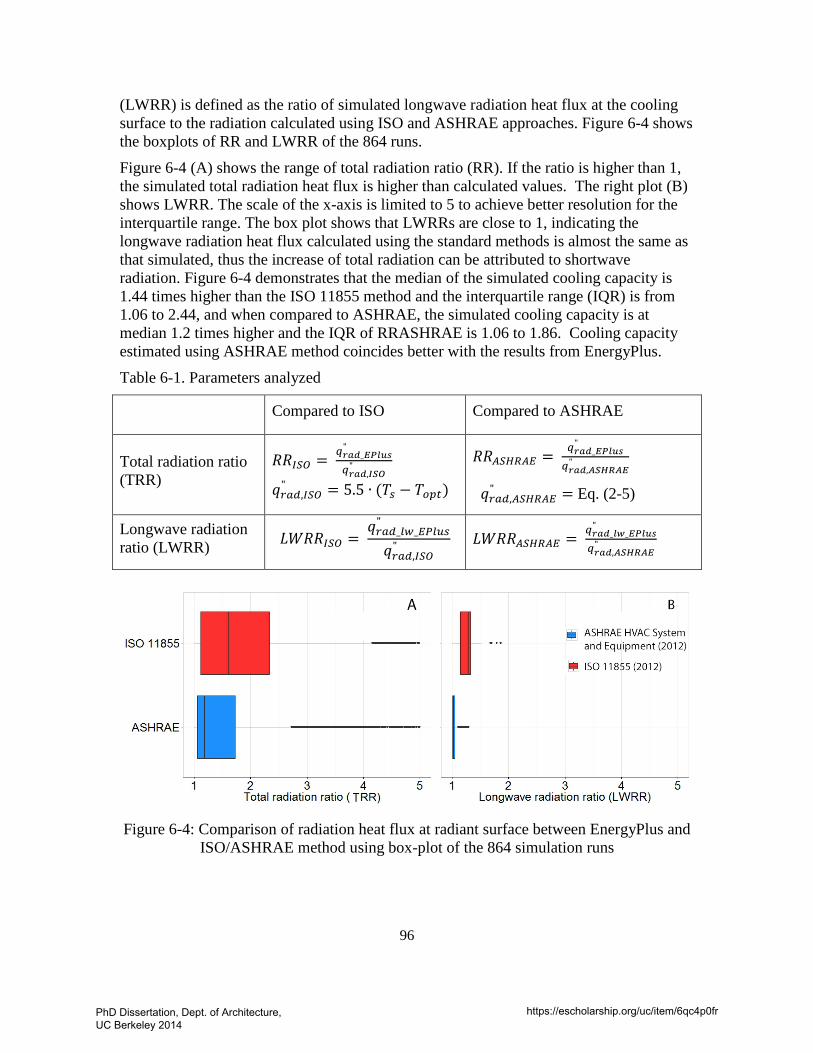
96

(LWRR) is defined as the ratio of simulated longwave radiation heat flux at the cooling surface to the radiation calculated using ISO and ASHRAE approaches. Figure 6-4 shows the boxplots of RR and LWRR of the 864 runs.

Figure 6-4 (A) shows the range of total radiation ratio (RR). If the ratio is higher than 1, the simulated total radiation heat flux is higher than calculated values. The right plot (B) shows LWRR. The scale of the x-axis is limited to 5 to achieve better resolution for the interquartile range. The box plot shows that LWRRs are close to 1, indicating the longwave radiation heat flux calculated using the standard methods is almost the same as that simulated, thus the increase of total radiation can be attributed to shortwave radiation. Figure 6-4 demonstrates that the median of the simulated cooling capacity is 1.44 times higher than the ISO 11855 method and the interquartile range (IQR) is from 1.06 to 2.44, and when compared to ASHRAE, the simulated cooling capacity is at median 1.2 times higher and the IQR of RRASHRAE is 1.06 to 1.86. Cooling capacity estimated using ASHRAE method coincides better with the results from EnergyPlus.

Table 6-1. Parameters analyzed

Compared to ISO Compared to ASHRAE

Total radiation ratio (TRR)

𝑅𝑅𝐼𝑆𝑂 = 𝑞𝑟𝑎𝑑_𝐸𝑃𝑙𝑢𝑠"

𝑞𝑟𝑎𝑑,𝐼𝑆𝑂"

𝑞𝑞𝑟𝑎𝑑,𝐼𝑆𝑂" = 5.5 ∙ (𝑇𝑠 − 𝑇𝑜𝑝𝑡)

𝑅𝑅𝐴𝑆𝐻𝑅𝐴𝐸 = 𝑞𝑟𝑎𝑑_𝐸𝑃𝑙𝑢𝑠"

𝑞𝑟𝑎𝑑,𝐴𝑆𝐻𝑅𝐴𝐸"

𝑞𝑞𝑟𝑎𝑑,𝐴𝑆𝐻𝑅𝐴𝐸" = Eq. (2-5)

Longwave radiation ratio (LWRR) 𝐿𝑊𝑅𝑅𝐼𝑆𝑂 =

𝑞𝑞𝑟𝑎𝑑_𝑙𝑤_𝐸𝑃𝑙𝑢𝑠"

𝑞𝑞𝑟𝑎𝑑,𝐼𝑆𝑂" 𝐿𝑊𝑅𝑅𝐴𝑆𝐻𝑅𝐴𝐸 = 𝑞𝑟𝑎𝑑_𝑙𝑤_𝐸𝑃𝑙𝑢𝑠

"

𝑞𝑟𝑎𝑑,𝐴𝑆𝐻𝑅𝐴𝐸"

Figure 6-4: Comparison of radiation heat flux at radiant surface between EnergyPlus and ISO/ASHRAE method using box-plot of the 864 simulation runs



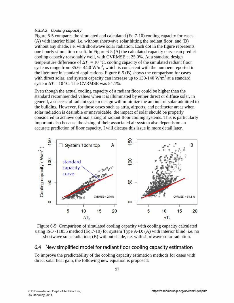
97

6.3.3.2 Cooling capacity Figure 6-5 compares the simulated and calculated (Eq.7-10) cooling capacity for cases: (A) with interior blind, i.e. without shortwave solar hitting the radiant floor, and (B) without any shade, i.e. with shortwave solar radiation. Each dot in the figure represents one hourly simulation result. In Figure 6-5 (A) the calculated capacity curve can predict cooling capacity reasonably well, with CVRMSE at 25.0%. At a standard design temperature difference of ∆Th = 10 °C, cooling capacity of the simulated radiant floor systems range from 35.6– 44.0 W/m2, which is consistent with the numbers reported in the literature in standard applications. Figure 6-5 (B) shows the comparison for cases with direct solar, and system capacity can increase up to 130-140 W/m2 at a standard system ∆T = 10 °C. The CVRMSE was 54.1%. Even though the actual cooling capacity of a radiant floor could be higher than the standard recommended values when it is illuminated by either direct or diffuse solar, in general, a successful radiant system design will minimize the amount of solar admitted to the building. However, for those cases such as atria, airports, and perimeter areas when solar radiation is desirable or unavoidable, the impact of solar should be properly considered to achieve optimal sizing of radiant floor cooling systems. This is particularly important also because the sizing of their associated air system also depends on an accurate prediction of floor capacity. I will discuss this issue in more detail later.

Figure 6-5: Comparison of simulated cooling capacity with cooling capacity calculated

using ISO -11855 method (Eq.7-10) for system Type A-D: (A) with interior blind, i.e. no shortwave solar radiation; (B) without shade, i.e. with shortwave solar radiation.

6.4 New simplified model for radiant floor cooling capacity estimation To improve the predictability of the cooling capacity estimation methods for cases with direct solar heat gain, the following new equation is proposed:



98

𝑞𝑞" = 𝐾 ∙ ∆𝑇ℎ + 𝑞𝑞𝑠𝑤_𝑠𝑜𝑙" Equation 6-6

𝑞𝑞𝑠𝑤_𝑠𝑜𝑙" is the cooling capacity enhancement caused by absorbing of direct solar

radiation. Equation 6-7 is the proposed correlation to calculate 𝑞𝑞𝑠𝑤_𝑠𝑜𝑙" and the derivation

of this correlation is described in the Appendix A.

𝑞𝑞𝑠𝑤_𝑠𝑜𝑙" = 1.993 ∙ (𝑞𝑞𝑠𝑜𝑙,𝑤𝑖𝑛" )

0.7476− 5.038 ∙ ( 𝑞𝑞𝑠𝑜𝑙,𝑤𝑖𝑛" ∙ ∆𝑇ℎ)

0.2793 Equation 6-7

Where, qsol,win" = total transmitted solar heat flux into the space; ∆𝑇 can be calculated by Equation 6-4. This model has an adjusted R2 = 0.92.

The 𝑞𝑞𝑠𝑜𝑙,𝑤𝑖𝑛" includes both the beam and diffuse solar heat flux that are transmitted through the windows into the space. If there is no complex fenestration system, i.e. shading devices or light shelf, it can be obtained by multiplying the incident solar heat flux on the window and the window’s total solar transmittance. If complex fenestration systems are installed, more advanced simulation tools may need to be used for the calculation.

Theoretically speaking, solar transmittance is a variable that is directionally and spectrally (wavelength) dependent. The calculation of total transmitted solar with high accuracy requires detailed information of window’s optical properties, which could be obtained using tools, such as the WINDOW 7.2 software developed by Lawrence Berkeley National Lab. However, in practice, there are usually simplifications. For example, in DOE-2 and with the simple glazing option in EnergyPlus, the total solar transmittance at normal incident is used. For designers who only have information about window’s solar heat gain coefficient (SHGC) and U values, the total solar transmittance at normal incident could be calculated using the regression models developed by researchers at Lawrence Berkeley National Lab (Arasteh et al. 2009) .

Note that the heat transfer process with incident solar radiation is highly dynamic; the proposed calculation method can be used for rough estimation of the system design capacity and is not intended to replace detailed dynamic simulation.

6.5 Implications for sizing of associated air system As mentioned before, radiant systems are typically configured as a hybrid with an air system, and the designers have to size the air system to provide supplemental cooling if the space total cooling load exceeds the maximum capacity of the radiant system. Thus, the desired capacity of the air system is directly related to the radiant system cooling capacity, and therefore underestimation of the radiant system capacity when solar load is significant can lead to oversizing of the air system. In this section, we conducted a new series of simulations of the hybrid radiant and air system, and the goals are to validate the applicability of the proposed approach to the estimation of radiant system cooling capacity and demonstrate how to use it for sizing of the associated air system.

The same single zone model described in Section 6.3 was used but with an idealized air system simulated to meet ventilation and latent loads and supplemental cooling



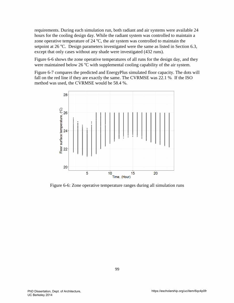
99

requirements. During each simulation run, both radiant and air systems were available 24 hours for the cooling design day. While the radiant system was controlled to maintain a zone operative temperature of 24 °C, the air system was controlled to maintain the setpoint at 26 °C. Design parameters investigated were the same as listed in Section 6.3, except that only cases without any shade were investigated (432 runs).

Figure 6-6 shows the zone operative temperatures of all runs for the design day, and they were maintained below 26 °C with supplemental cooling capability of the air system.

Figure 6-7 compares the predicted and EnergyPlus simulated floor capacity. The dots will fall on the red line if they are exactly the same. The CVRMSE was 22.1 %. If the ISO method was used, the CVRMSE would be 58.4 %.

Figure 6-6: Zone operative temperature ranges during all simulation runs



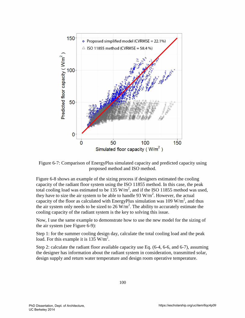
100

Figure 6-7: Comparison of EnergyPlus simulated capacity and predicted capacity using proposed method and ISO method.

Figure 6-8 shows an example of the sizing process if designers estimated the cooling capacity of the radiant floor system using the ISO 11855 method. In this case, the peak total cooling load was estimated to be 135 W/m2, and if the ISO 11855 method was used, they have to size the air system to be able to handle 93 W/m2. However, the actual capacity of the floor as calculated with EnergyPlus simulation was 109 W/m2, and thus the air system only needs to be sized to 26 W/m2. The ability to accurately estimate the cooling capacity of the radiant system is the key to solving this issue.

Now, I use the same example to demonstrate how to use the new model for the sizing of the air system (see Figure 6-9):

Step 1: for the summer cooling design day, calculate the total cooling load and the peak load. For this example it is 135 W/m2.

Step 2: calculate the radiant floor available capacity use Eq. (6-4, 6-6, and 6-7), assuming the designer has information about the radiant system in consideration, transmitted solar, design supply and return water temperature and design room operative temperature.



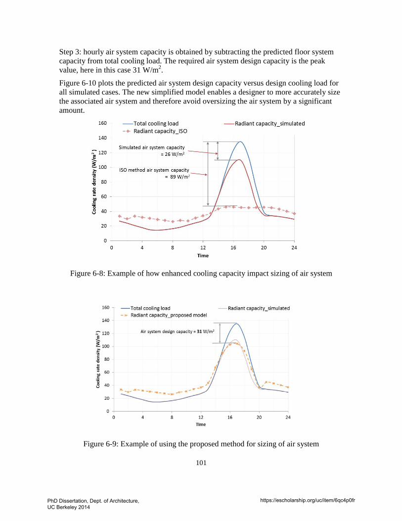
101

Step 3: hourly air system capacity is obtained by subtracting the predicted floor system capacity from total cooling load. The required air system design capacity is the peak value, here in this case 31 W/m2.

Figure 6-10 plots the predicted air system design capacity versus design cooling load for all simulated cases. The new simplified model enables a designer to more accurately size the associated air system and therefore avoid oversizing the air system by a significant amount.

Figure 6-8: Example of how enhanced cooling capacity impact sizing of air system

Figure 6-9: Example of using the proposed method for sizing of air system



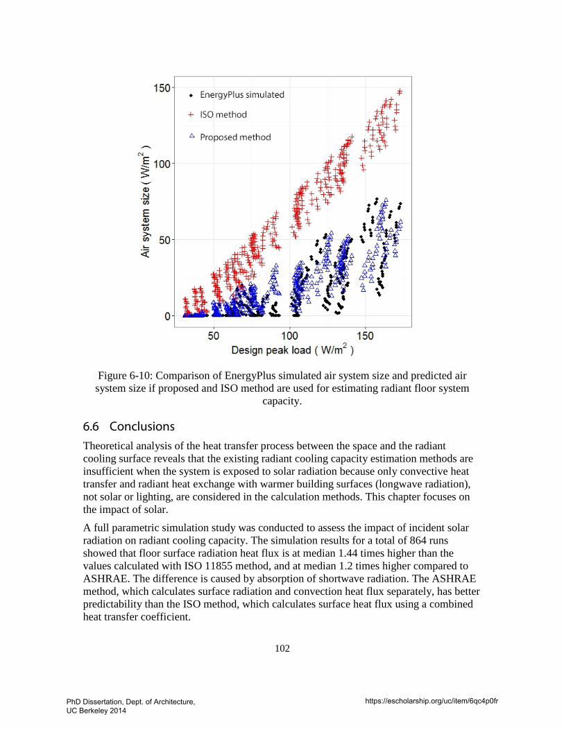
102

Figure 6-10: Comparison of EnergyPlus simulated air system size and predicted air system size if proposed and ISO method are used for estimating radiant floor system

capacity.

6.6 Conclusions Theoretical analysis of the heat transfer process between the space and the radiant cooling surface reveals that the existing radiant cooling capacity estimation methods are insufficient when the system is exposed to solar radiation because only convective heat transfer and radiant heat exchange with warmer building surfaces (longwave radiation), not solar or lighting, are considered in the calculation methods. This chapter focuses on the impact of solar.

A full parametric simulation study was conducted to assess the impact of incident solar radiation on radiant cooling capacity. The simulation results for a total of 864 runs showed that floor surface radiation heat flux is at median 1.44 times higher than the values calculated with ISO 11855 method, and at median 1.2 times higher compared to ASHRAE. The difference is caused by absorption of shortwave radiation. The ASHRAE method, which calculates surface radiation and convection heat flux separately, has better predictability than the ISO method, which calculates surface heat flux using a combined heat transfer coefficient.



103

The simulation results also confirm that the ISO 11855 cooling capacity estimation method does not apply to cases when there is solar load. When interior blinds are installed to block solar gain, ISO 11855 cooling capacity estimation methods can well predict the system performance. When there is no shading system, the system capacity can increase up to 130-140 W/m2 at a standard system temperature difference of 10 °C.

To improve the predictability of the cooling capacity estimation methods for cases with direct solar heat gain, a new equation is proposed to estimate system capacity enhancement due to direct solar absorption. The new simplified model calculates the enhanced capacity as a function of window transmitted solar radiation and a mean temperature differences between the hydronic loop and room operative temperature. The new regression model has an adjusted R2

adj = 0.92.

This paper also addressed the question regarding sizing of the associated air system in cases when radiant system capacity are enhanced by solar. The new model was used to predict radiant floor system capacity, and when compared with EnergyPlus simulated cooling capacity, the CVRMSE was 22.1 %. The new simplified model enables designers to more accurately size the associated air system and therefore avoid oversizing the air system by a significant amount.



104

7 CONTROL OF HEAVYWEIGH RADIANT SLAB SYSTEMS

7.1 Introduction For the design of heavyweight radiant slab systems, control strategies should be taken into account for load analysis and equipment sizing. This chapter investigates the energy and comfort benefits of advanced control optimization techniques, particularly model-based predictive control (MPC) method, when applied to a heavyweight embedded surface system. The objectives are to:1) create a simplified dynamic model of a radiant slab system for easy implementation in a model predictive controller, 2) implement the model based predictive controller for a test building with a radiant slab system, and 3) compare its energy and thermal comfort performance with a fine-tuned heuristic rule-based control method.

7.2 Model based predictive control (MPC) Model predictive control was first used in the chemical process industry in the 1960s. More recently, model predictive control (MPC) has become popular in the building industry. The desire is to optimize operation based on a short-term prediction of weather and building utilization to yield energy and cost savings through minimization of an objective function over a predictive horizon. For example, building thermal mass control to respond to utility pricing signals, thermal load prediction for uniform chiller loading and improved part-load performance, and predicted occupant behavior integrated in mixed mode building control.

The design of MPC is based on three main steps: (1) at each sampling time, t, the use of a model to predict the output vector k step in the future, 𝑦(𝑡𝑡|𝑡𝑡),𝑦(𝑡𝑡 + 𝑘|𝑡𝑡) (the top diagram of Figure 7-1); (2) an open-loop optimal control problem is solved online over a finite horizon, and the computed optimal manipulated input signal is applied to the process only during the following sampling interval [𝑡𝑡, 𝑡𝑡 + 1]; (3) at next sampling time at 𝑡𝑡 + 1, a new optimal control problem based on new measurements of the state is solved over a shifted horizon (as shown in the bottom diagram of Figure 7-1).

Depending on the application and implementation strategy, the types of model required for MPC can be different. A good review and comparison of different modeling methods used for model-based control can be found in the article by Henze (2011). In this article, he differentiates the model types depending on the type or the physical relevance of the parameters. Here is a brief summary:

• White-box model: Physical model with exclusively meaningful parameters (internal structure of the process is modelled). They are based on a physical description of the system, and are generally known as “first principle” models, where the classical energy and mass conservation laws are usually applied. The amount of effort needed to develop a white box model depends on the amount of detail in the model. A very simple white box may be developed to accurately represent system behavior. The values of white box model parameters are available over a wide range of



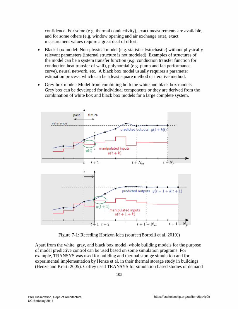
105

confidence. For some (e.g. thermal conductivity), exact measurements are available, and for some others (e.g. window opening and air exchange rate), exact measurement values require a great deal of effort.

• Black-box model: Non-physical model (e.g. statistical/stochastic) without physically relevant parameters (internal structure is not modeled). Examples of structures of the model can be a system transfer function (e.g. conduction transfer function for conduction heat transfer of wall), polynomial (e.g. pump and fan performance curve), neural network, etc. A black box model usually requires a parameter estimation process, which can be a least square method or iterative method.

• Grey-box model: Model from combining both the white and black box models. Grey box can be developed for individual components or they are derived from the combination of white box and black box models for a large complete system.

Figure 7-1: Receding Horizon Idea (source:(Borrelli et al. 2010))

Apart from the white, gray, and black box model, whole building models for the purpose of model predictive control can be used based on some simulation programs. For example, TRANSYS was used for building and thermal storage simulation and for experimental implementation by Henze et al. in their thermal storage study in buildings (Henze and Krarti 2005). Coffey used TRANSYS for simulation based studies of demand



106

response by changing room air temperature setpoint (Coffey 2008). EnergyPlus could also be used. The group Henze led has recently taken a white box model approach to mixed-mode building control(May-Ostendorp et al. 2011). Their goal is to extract control rule utilizing the results from a MPC study using Matlab/EnergyPlus..

As noted by Henze and Neumann (2011), model-based control can usually be accomplished by the following two ways: offline optimization and online optimization. High fidelity models can be used for both but more desirable in the latter case.

For online optimization, model-based predictive controllers aim to optimize the system by accounting for current and future building operation boundary conditions, e.g. in terms of weather, indoor climate or presence of occupants. From this information, the actual operation can be optimized, theoretically every time step (every hour, for example). Yet this type of optimization requires significant effort and a close coupling with the building automation system. In this case, somewhat lower order models are usually used. In offline optimization, the building operation is optimized externally, i.e., the building is simulated offline, where certain user profiles and a suitable weather data set are assumed. Such studies can then be used to inform the development of conventional control rules or control table that can approximate the optimal control in some cases but be simpler for implementation (Coffey 2011, May-Ostendorp et al. 2011). The aim is to determine general control strategies for the systems in the building in order to minimize annual energy consumption or costs. In those cases, high fidelity models are usually used.

For this study, a simplified first-order dynamic model is developed for online optimization implementation.

7.3 Methodology To assess the efficacy of various control techniques for radiant slab systems, we must create a flexible testbed with which to implement the controllers. A calibrated EnergyPlus model of a test building conditioned by a radiant system was developed. The procedure for the work is outlined below.

• Create and calibrate an EnergyPlus model of the case study building and the associated HVAC system.

• Derive simplified dynamic models of the EnergyPlus model for MPC controller design.

• Design MPC controller for the radiant system.

• Implement and test a fine-tuned rule-based control strategy and the MPC controller on the EnergyPlus model.

• Create and compare metrics for thermal comfort and energy consumption of the controllers.

There are three main advantages of using an EnergyPlus model of a real building versus a fictitious building for the test: 1) the radiant system model in EnergyPlus can be validated against field measurement data; 2) the utility bill and monitored long term data of a real



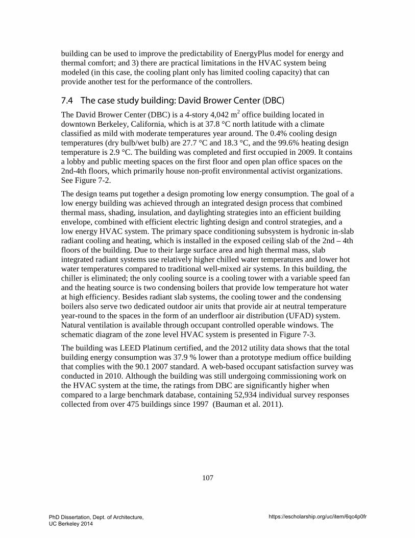
107

building can be used to improve the predictability of EnergyPlus model for energy and thermal comfort; and 3) there are practical limitations in the HVAC system being modeled (in this case, the cooling plant only has limited cooling capacity) that can provide another test for the performance of the controllers.

7.4 The case study building: David Brower Center (DBC) The David Brower Center (DBC) is a 4-story 4,042 m2 office building located in downtown Berkeley, California, which is at 37.8 °C north latitude with a climate classified as mild with moderate temperatures year around. The 0.4% cooling design temperatures (dry bulb/wet bulb) are 27.7 °C and 18.3 °C, and the 99.6% heating design temperature is 2.9 °C. The building was completed and first occupied in 2009. It contains a lobby and public meeting spaces on the first floor and open plan office spaces on the 2nd-4th floors, which primarily house non-profit environmental activist organizations. See Figure 7-2.

The design teams put together a design promoting low energy consumption. The goal of a low energy building was achieved through an integrated design process that combined thermal mass, shading, insulation, and daylighting strategies into an efficient building envelope, combined with efficient electric lighting design and control strategies, and a low energy HVAC system. The primary space conditioning subsystem is hydronic in-slab radiant cooling and heating, which is installed in the exposed ceiling slab of the 2nd – 4th floors of the building. Due to their large surface area and high thermal mass, slab integrated radiant systems use relatively higher chilled water temperatures and lower hot water temperatures compared to traditional well-mixed air systems. In this building, the chiller is eliminated; the only cooling source is a cooling tower with a variable speed fan and the heating source is two condensing boilers that provide low temperature hot water at high efficiency. Besides radiant slab systems, the cooling tower and the condensing boilers also serve two dedicated outdoor air units that provide air at neutral temperature year-round to the spaces in the form of an underfloor air distribution (UFAD) system. Natural ventilation is available through occupant controlled operable windows. The schematic diagram of the zone level HVAC system is presented in Figure 7-3.

The building was LEED Platinum certified, and the 2012 utility data shows that the total building energy consumption was 37.9 % lower than a prototype medium office building that complies with the 90.1 2007 standard. A web-based occupant satisfaction survey was conducted in 2010. Although the building was still undergoing commissioning work on the HVAC system at the time, the ratings from DBC are significantly higher when compared to a large benchmark database, containing 52,934 individual survey responses collected from over 475 buildings since 1997 (Bauman et al. 2011).



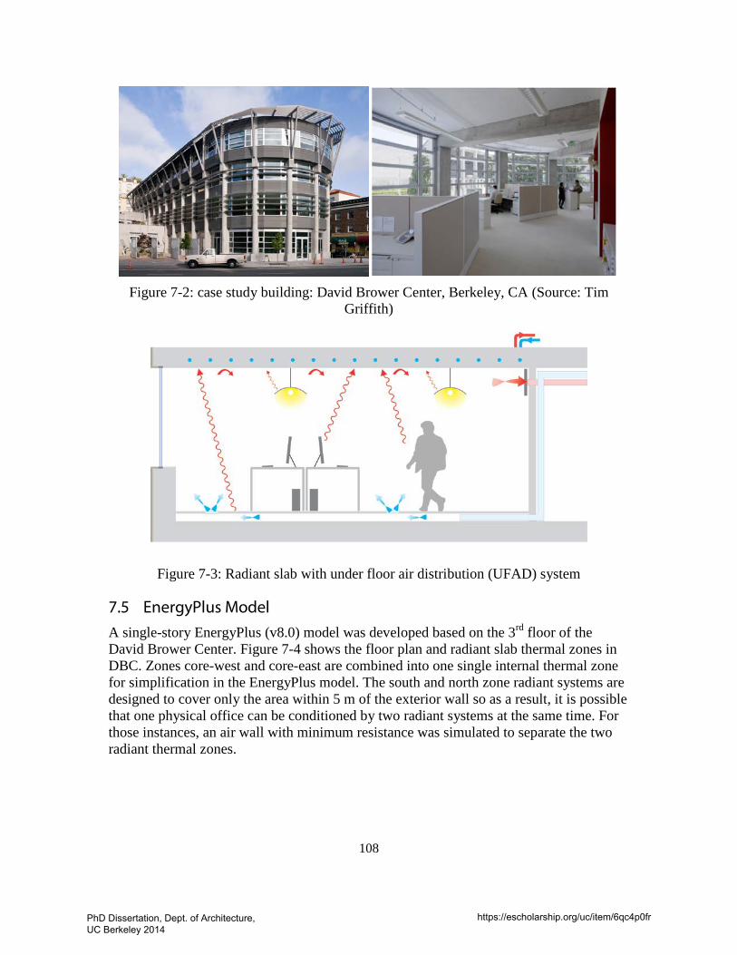
108

Figure 7-2: case study building: David Brower Center, Berkeley, CA (Source: Tim

Griffith)

Figure 7-3: Radiant slab with under floor air distribution (UFAD) system

7.5 EnergyPlus Model A single-story EnergyPlus (v8.0) model was developed based on the 3rd floor of the David Brower Center. Figure 7-4 shows the floor plan and radiant slab thermal zones in DBC. Zones core-west and core-east are combined into one single internal thermal zone for simplification in the EnergyPlus model. The south and north zone radiant systems are designed to cover only the area within 5 m of the exterior wall so as a result, it is possible that one physical office can be conditioned by two radiant systems at the same time. For those instances, an air wall with minimum resistance was simulated to separate the two radiant thermal zones.



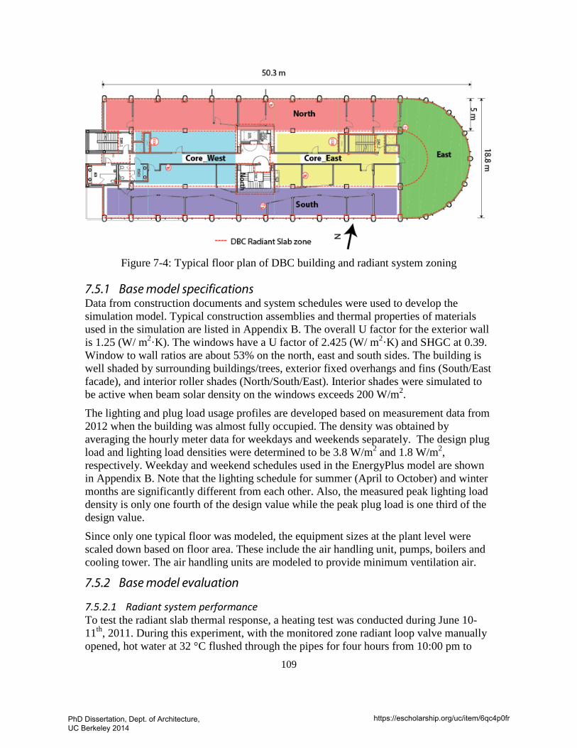
109

Figure 7-4: Typical floor plan of DBC building and radiant system zoning

7.5.1 Base model specifications Data from construction documents and system schedules were used to develop the simulation model. Typical construction assemblies and thermal properties of materials used in the simulation are listed in Appendix B. The overall U factor for the exterior wall is 1.25 (W/ m2·K). The windows have a U factor of 2.425 (W/ m2·K) and SHGC at 0.39. Window to wall ratios are about 53% on the north, east and south sides. The building is well shaded by surrounding buildings/trees, exterior fixed overhangs and fins (South/East facade), and interior roller shades (North/South/East). Interior shades were simulated to be active when beam solar density on the windows exceeds 200 W/m2.

The lighting and plug load usage profiles are developed based on measurement data from 2012 when the building was almost fully occupied. The density was obtained by averaging the hourly meter data for weekdays and weekends separately. The design plug load and lighting load densities were determined to be 3.8 W/m2 and 1.8 W/m2, respectively. Weekday and weekend schedules used in the EnergyPlus model are shown in Appendix B. Note that the lighting schedule for summer (April to October) and winter months are significantly different from each other. Also, the measured peak lighting load density is only one fourth of the design value while the peak plug load is one third of the design value.

Since only one typical floor was modeled, the equipment sizes at the plant level were scaled down based on floor area. These include the air handling unit, pumps, boilers and cooling tower. The air handling units are modeled to provide minimum ventilation air.

7.5.2 Base model evaluation

7.5.2.1 Radiant system performance To test the radiant slab thermal response, a heating test was conducted during June 10-11th, 2011. During this experiment, with the monitored zone radiant loop valve manually opened, hot water at 32 °C flushed through the pipes for four hours from 10:00 pm to



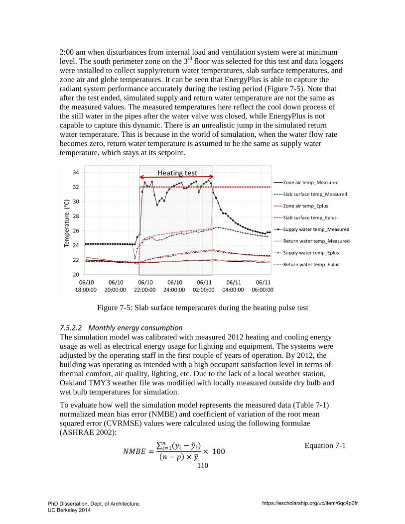
110

2:00 am when disturbances from internal load and ventilation system were at minimum level. The south perimeter zone on the 3rd floor was selected for this test and data loggers were installed to collect supply/return water temperatures, slab surface temperatures, and zone air and globe temperatures. It can be seen that EnergyPlus is able to capture the radiant system performance accurately during the testing period (Figure 7-5). Note that after the test ended, simulated supply and return water temperature are not the same as the measured values. The measured temperatures here reflect the cool down process of the still water in the pipes after the water valve was closed, while EnergyPlus is not capable to capture this dynamic. There is an unrealistic jump in the simulated return water temperature. This is because in the world of simulation, when the water flow rate becomes zero, return water temperature is assumed to be the same as supply water temperature, which stays at its setpoint.

Figure 7-5: Slab surface temperatures during the heating pulse test

7.5.2.2 Monthly energy consumption The simulation model was calibrated with measured 2012 heating and cooling energy usage as well as electrical energy usage for lighting and equipment. The systems were adjusted by the operating staff in the first couple of years of operation. By 2012, the building was operating as intended with a high occupant satisfaction level in terms of thermal comfort, air quality, lighting, etc. Due to the lack of a local weather station, Oakland TMY3 weather file was modified with locally measured outside dry bulb and wet bulb temperatures for simulation.

To evaluate how well the simulation model represents the measured data (Table 7-1) normalized mean bias error (NMBE) and coefficient of variation of the root mean squared error (CVRMSE) values were calculated using the following formulae (ASHRAE 2002):

𝑁𝑀𝐵𝐸 =∑ (𝑦𝑖 − 𝑦�𝑖𝑛𝑖=1 )

(𝑛 − 𝑝) × 𝑦�× 100

Equation 7-1



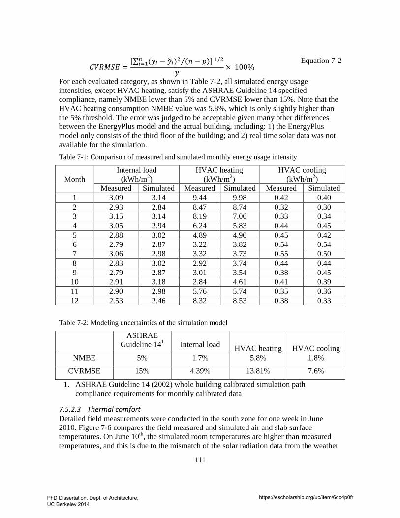
111

𝐶𝑉𝑅𝑀𝑆𝐸 =[∑ (𝑦𝑖 − 𝑦�𝑖)2𝑛

𝑖=1 (𝑛 − 𝑝)⁄ ] 1/2

𝑦�× 100%

Equation 7-2

For each evaluated category, as shown in Table 7-2, all simulated energy usage intensities, except HVAC heating, satisfy the ASHRAE Guideline 14 specified compliance, namely NMBE lower than 5% and CVRMSE lower than 15%. Note that the HVAC heating consumption NMBE value was 5.8%, which is only slightly higher than the 5% threshold. The error was judged to be acceptable given many other differences between the EnergyPlus model and the actual building, including: 1) the EnergyPlus model only consists of the third floor of the building; and 2) real time solar data was not available for the simulation. Table 7-1: Comparison of measured and simulated monthly energy usage intensity

Month Internal load

(kWh/m2) HVAC heating

(kWh/m2) HVAC cooling

(kWh/m2) Measured Simulated Measured Simulated Measured Simulated

1 3.09 3.14 9.44 9.98 0.42 0.40 2 2.93 2.84 8.47 8.74 0.32 0.30 3 3.15 3.14 8.19 7.06 0.33 0.34 4 3.05 2.94 6.24 5.83 0.44 0.45 5 2.88 3.02 4.89 4.90 0.45 0.42 6 2.79 2.87 3.22 3.82 0.54 0.54 7 3.06 2.98 3.32 3.73 0.55 0.50 8 2.83 3.02 2.92 3.74 0.44 0.44 9 2.79 2.87 3.01 3.54 0.38 0.45 10 2.91 3.18 2.84 4.61 0.41 0.39 11 2.90 2.98 5.76 5.74 0.35 0.36 12 2.53 2.46 8.32 8.53 0.38 0.33

Table 7-2: Modeling uncertainties of the simulation model

ASHRAE

Guideline 141 Internal load HVAC heating HVAC cooling NMBE 5% 1.7% 5.8% 1.8%

CVRMSE 15% 4.39% 13.81% 7.6%

1. ASHRAE Guideline 14 (2002) whole building calibrated simulation path compliance requirements for monthly calibrated data

7.5.2.3 Thermal comfort Detailed field measurements were conducted in the south zone for one week in June 2010. Figure 7-6 compares the field measured and simulated air and slab surface temperatures. On June 10th, the simulated room temperatures are higher than measured temperatures, and this is due to the mismatch of the solar radiation data from the weather



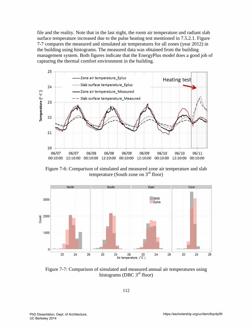
112

file and the reality. Note that in the last night, the room air temperature and radiant slab surface temperature increased due to the pulse heating test mentioned in 7.5.2.1. Figure 7-7 compares the measured and simulated air temperatures for all zones (year 2012) in the building using histograms. The measured data was obtained from the building management system. Both figures indicate that the EnergyPlus model does a good job of capturing the thermal comfort environment in the building.

Figure 7-6: Comparison of simulated and measured zone air temperature and slab temperature (South zone on 3rd floor)

Figure 7-7: Comparison of simulated and measured annual air temperatures using histograms (DBC 3rd floor)



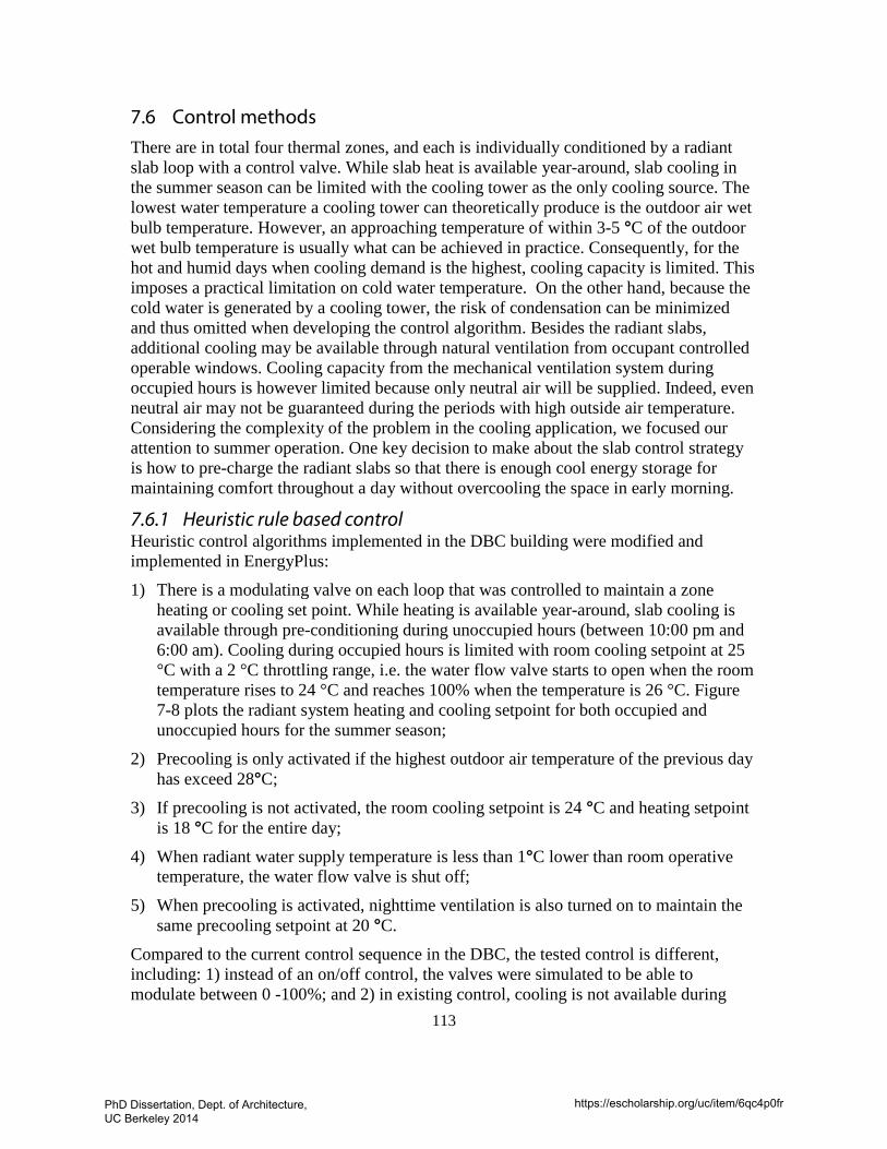
113

7.6 Control methods There are in total four thermal zones, and each is individually conditioned by a radiant slab loop with a control valve. While slab heat is available year-around, slab cooling in the summer season can be limited with the cooling tower as the only cooling source. The lowest water temperature a cooling tower can theoretically produce is the outdoor air wet bulb temperature. However, an approaching temperature of within 3-5 °C of the outdoor wet bulb temperature is usually what can be achieved in practice. Consequently, for the hot and humid days when cooling demand is the highest, cooling capacity is limited. This imposes a practical limitation on cold water temperature. On the other hand, because the cold water is generated by a cooling tower, the risk of condensation can be minimized and thus omitted when developing the control algorithm. Besides the radiant slabs, additional cooling may be available through natural ventilation from occupant controlled operable windows. Cooling capacity from the mechanical ventilation system during occupied hours is however limited because only neutral air will be supplied. Indeed, even neutral air may not be guaranteed during the periods with high outside air temperature. Considering the complexity of the problem in the cooling application, we focused our attention to summer operation. One key decision to make about the slab control strategy is how to pre-charge the radiant slabs so that there is enough cool energy storage for maintaining comfort throughout a day without overcooling the space in early morning.

7.6.1 Heuristic rule based control Heuristic control algorithms implemented in the DBC building were modified and implemented in EnergyPlus:

1) There is a modulating valve on each loop that was controlled to maintain a zone heating or cooling set point. While heating is available year-around, slab cooling is available through pre-conditioning during unoccupied hours (between 10:00 pm and 6:00 am). Cooling during occupied hours is limited with room cooling setpoint at 25 °C with a 2 °C throttling range, i.e. the water flow valve starts to open when the room temperature rises to 24 °C and reaches 100% when the temperature is 26 °C. Figure 7-8 plots the radiant system heating and cooling setpoint for both occupied and unoccupied hours for the summer season;

2) Precooling is only activated if the highest outdoor air temperature of the previous day has exceed 28°C;

3) If precooling is not activated, the room cooling setpoint is 24 °C and heating setpoint is 18 °C for the entire day;

4) When radiant water supply temperature is less than 1°C lower than room operative temperature, the water flow valve is shut off;

5) When precooling is activated, nighttime ventilation is also turned on to maintain the same precooling setpoint at 20 °C.

Compared to the current control sequence in the DBC, the tested control is different, including: 1) instead of an on/off control, the valves were simulated to be able to modulate between 0 -100%; and 2) in existing control, cooling is not available during



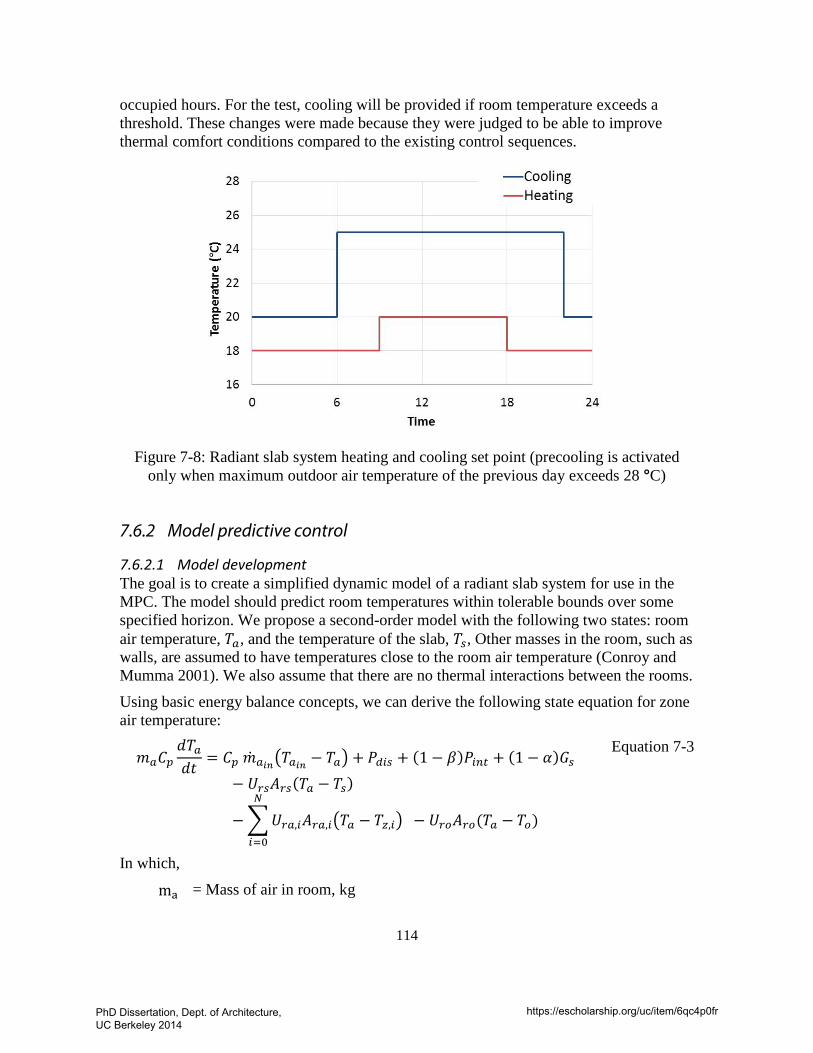
114

occupied hours. For the test, cooling will be provided if room temperature exceeds a threshold. These changes were made because they were judged to be able to improve thermal comfort conditions compared to the existing control sequences.

Figure 7-8: Radiant slab system heating and cooling set point (precooling is activated

only when maximum outdoor air temperature of the previous day exceeds 28 °C)

7.6.2 Model predictive control

7.6.2.1 Model development The goal is to create a simplified dynamic model of a radiant slab system for use in the MPC. The model should predict room temperatures within tolerable bounds over some specified horizon. We propose a second-order model with the following two states: room air temperature, 𝑇𝑎, and the temperature of the slab, 𝑇𝑠, Other masses in the room, such as walls, are assumed to have temperatures close to the room air temperature (Conroy and Mumma 2001). We also assume that there are no thermal interactions between the rooms.

Using basic energy balance concepts, we can derive the following state equation for zone air temperature:

𝑚𝑎𝐶𝑝𝑑𝑇𝑎𝑑𝑡𝑡

= 𝐶𝑝 ��𝑎𝑖𝑛�𝑇𝑎𝑖𝑛 − 𝑇𝑎� + 𝑃𝑃𝑑𝑖𝑠 + (1 − 𝛽)𝑃𝑃𝑖𝑛𝑡 + (1 − 𝛼)𝐺𝑠− 𝑈𝑟𝑠𝐴𝑟𝑠(𝑇𝑎 − 𝑇𝑠)

−�𝑈𝑟𝑎,𝑖𝐴𝑟𝑎,𝑖�𝑇𝑎 − 𝑇𝑧,𝑖� − 𝑈𝑟𝑜𝐴𝑟𝑜(𝑇𝑎 − 𝑇𝑜)𝑁

𝑖=0

Equation 7-3

In which,

ma = Mass of air in room, kg



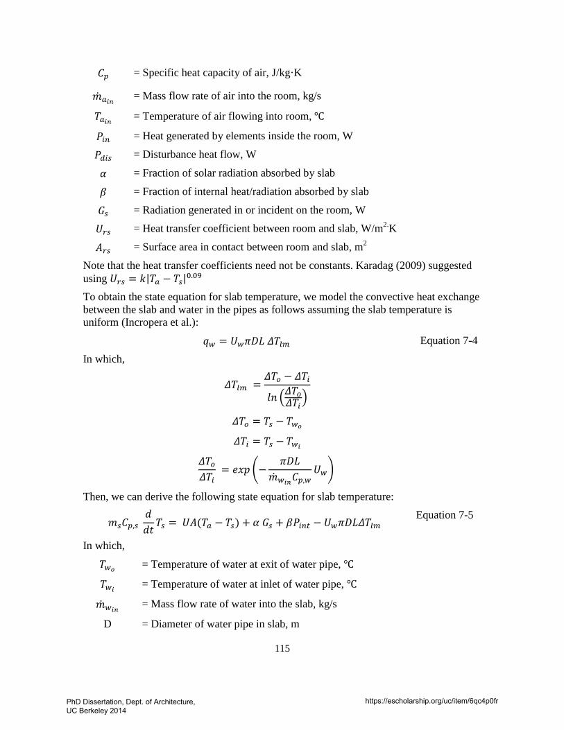
115

𝐶𝑝 = Specific heat capacity of air, J/kg·K

��𝑎𝑖𝑛 = Mass flow rate of air into the room, kg/s

𝑇𝑎𝑖𝑛 = Temperature of air flowing into room, ℃

𝑃𝑃𝑖𝑛 = Heat generated by elements inside the room, W

𝑃𝑃𝑑𝑖𝑠 = Disturbance heat flow, W

𝛼 = Fraction of solar radiation absorbed by slab

𝛽 = Fraction of internal heat/radiation absorbed by slab

𝐺𝑠 = Radiation generated in or incident on the room, W

𝑈𝑟𝑠 = Heat transfer coefficient between room and slab, W/m2.K

𝐴𝑟𝑠 = Surface area in contact between room and slab, m2

Note that the heat transfer coefficients need not be constants. Karadag (2009) suggested using 𝑈𝑟𝑠 = 𝑘|𝑇𝑎 − 𝑇𝑠|0.09 To obtain the state equation for slab temperature, we model the convective heat exchange between the slab and water in the pipes as follows assuming the slab temperature is uniform (Incropera et al.):

𝑞𝑞𝑤 = 𝑈𝑤𝜋𝐷𝐿 𝛥𝑇𝑙𝑚 Equation 7-4

In which,

𝛥𝑇𝑙𝑚 =𝛥𝑇𝑜 − 𝛥𝑇𝑖

𝑙𝑛 �𝛥𝑇𝑜𝛥𝑇𝑖�

𝛥𝑇𝑜 = 𝑇𝑠 − 𝑇𝑤𝑜

𝛥𝑇𝑖 = 𝑇𝑠 − 𝑇𝑤𝑖

𝛥𝑇𝑜𝛥𝑇𝑖

= 𝑒𝑥𝑝 �−𝜋𝐷𝐿

��𝑤𝑖𝑛𝐶𝑝,𝑤𝑈𝑤�

Then, we can derive the following state equation for slab temperature:

𝑚𝑠𝐶𝑝,𝑠 𝑑𝑑𝑡𝑡𝑇𝑠 = 𝑈𝐴(𝑇𝑎 − 𝑇𝑠) + 𝛼 𝐺𝑠 + 𝛽𝑃𝑃𝑖𝑛𝑡 − 𝑈𝑤𝜋𝐷𝐿𝛥𝑇𝑙𝑚

Equation 7-5

In which,

𝑇𝑤𝑜 = Temperature of water at exit of water pipe, ℃

𝑇𝑤𝑖 = Temperature of water at inlet of water pipe, ℃

��𝑤𝑖𝑛 = Mass flow rate of water into the slab, kg/s

D = Diameter of water pipe in slab, m



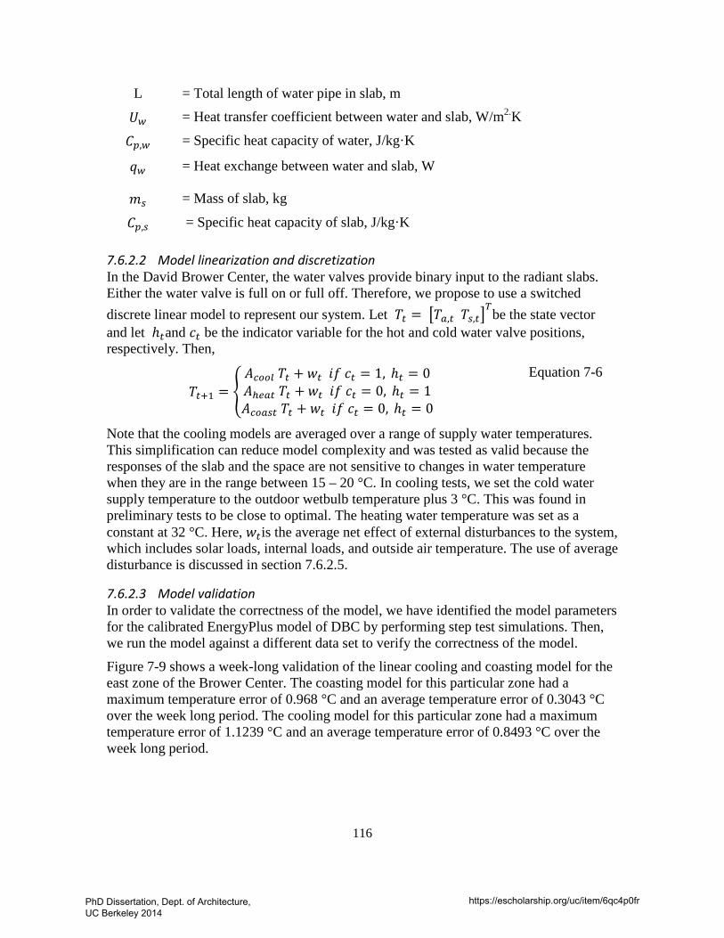
116

L = Total length of water pipe in slab, m

𝑈𝑤 = Heat transfer coefficient between water and slab, W/m2.K

𝐶𝑝,𝑤 = Specific heat capacity of water, J/kg·K

𝑞𝑞𝑤 = Heat exchange between water and slab, W

𝑚𝑠 = Mass of slab, kg

𝐶𝑝,𝑠 = Specific heat capacity of slab, J/kg·K

7.6.2.2 Model linearization and discretization In the David Brower Center, the water valves provide binary input to the radiant slabs. Either the water valve is full on or full off. Therefore, we propose to use a switched discrete linear model to represent our system. Let 𝑇𝑡 = �𝑇𝑎,𝑡 𝑇𝑠,𝑡�

𝑇be the state vector

and let ℎ𝑡and 𝑐𝑡 be the indicator variable for the hot and cold water valve positions, respectively. Then,

𝑇𝑡+1 = �𝐴𝑐𝑜𝑜𝑙 𝑇𝑡 + 𝑤𝑡 𝑎𝑎𝑠𝑠 𝑐𝑡 = 1, ℎ𝑡 = 0𝐴ℎ𝑒𝑎𝑡 𝑇𝑡 + 𝑤𝑡 𝑎𝑎𝑠𝑠 𝑐𝑡 = 0, ℎ𝑡 = 1𝐴𝑐𝑜𝑎𝑠𝑡 𝑇𝑡 + 𝑤𝑡 𝑎𝑎𝑠𝑠 𝑐𝑡 = 0, ℎ𝑡 = 0

Equation 7-6

Note that the cooling models are averaged over a range of supply water temperatures. This simplification can reduce model complexity and was tested as valid because the responses of the slab and the space are not sensitive to changes in water temperature when they are in the range between 15 – 20 °C. In cooling tests, we set the cold water supply temperature to the outdoor wetbulb temperature plus 3 °C. This was found in preliminary tests to be close to optimal. The heating water temperature was set as a constant at 32 °C. Here, 𝑤𝑡is the average net effect of external disturbances to the system, which includes solar loads, internal loads, and outside air temperature. The use of average disturbance is discussed in section 7.6.2.5.

7.6.2.3 Model validation In order to validate the correctness of the model, we have identified the model parameters for the calibrated EnergyPlus model of DBC by performing step test simulations. Then, we run the model against a different data set to verify the correctness of the model.

Figure 7-9 shows a week-long validation of the linear cooling and coasting model for the east zone of the Brower Center. The coasting model for this particular zone had a maximum temperature error of 0.968 °C and an average temperature error of 0.3043 °C over the week long period. The cooling model for this particular zone had a maximum temperature error of 1.1239 °C and an average temperature error of 0.8493 °C over the week long period.



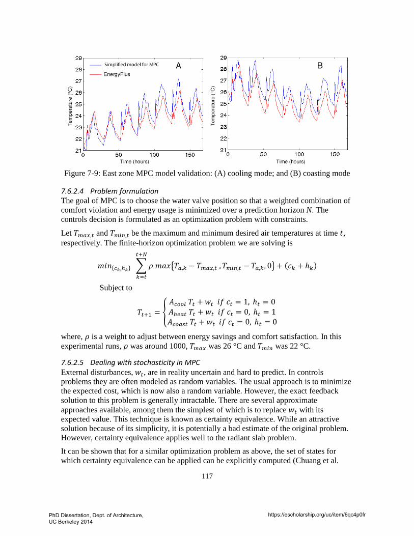
117

Figure 7-9: East zone MPC model validation: (A) cooling mode; and (B) coasting mode

7.6.2.4 Problem formulation The goal of MPC is to choose the water valve position so that a weighted combination of comfort violation and energy usage is minimized over a prediction horizon N. The controls decision is formulated as an optimization problem with constraints.

Let 𝑇𝑚𝑎𝑥,𝑡 and 𝑇𝑚𝑖𝑛,𝑡 be the maximum and minimum desired air temperatures at time 𝑡𝑡, respectively. The finite-horizon optimization problem we are solving is

𝑚𝑎𝑎𝑛{𝑐𝑘,ℎ𝑘} �𝜌 𝑚𝑎𝑎𝑥�𝑇𝑎,𝑘 − 𝑇𝑚𝑎𝑥,𝑡 ,𝑇𝑚𝑖𝑛,𝑡 − 𝑇𝑎,𝑘, 0�𝑡+𝑁

𝑘=𝑡

+ (𝑐𝑘 + ℎ𝑘)

Subject to

𝑇𝑡+1 = �𝐴𝑐𝑜𝑜𝑙 𝑇𝑡 + 𝑤𝑡 𝑎𝑎𝑠𝑠 𝑐𝑡 = 1, ℎ𝑡 = 0𝐴ℎ𝑒𝑎𝑡 𝑇𝑡 + 𝑤𝑡 𝑎𝑎𝑠𝑠 𝑐𝑡 = 0, ℎ𝑡 = 1𝐴𝑐𝑜𝑎𝑠𝑡 𝑇𝑡 + 𝑤𝑡 𝑎𝑎𝑠𝑠 𝑐𝑡 = 0, ℎ𝑡 = 0

where, 𝜌 is a weight to adjust between energy savings and comfort satisfaction. In this experimental runs, 𝜌 was around 1000, 𝑇𝑚𝑎𝑥 was 26 °C and 𝑇𝑚𝑖𝑛 was 22 °C.

7.6.2.5 Dealing with stochasticity in MPC External disturbances, 𝑤𝑡, are in reality uncertain and hard to predict. In controls problems they are often modeled as random variables. The usual approach is to minimize the expected cost, which is now also a random variable. However, the exact feedback solution to this problem is generally intractable. There are several approximate approaches available, among them the simplest of which is to replace 𝑤𝑡 with its expected value. This technique is known as certainty equivalence. While an attractive solution because of its simplicity, it is potentially a bad estimate of the original problem. However, certainty equivalence applies well to the radiant slab problem.

It can be shown that for a similar optimization problem as above, the set of states for which certainty equivalence can be applied can be explicitly computed (Chuang et al.



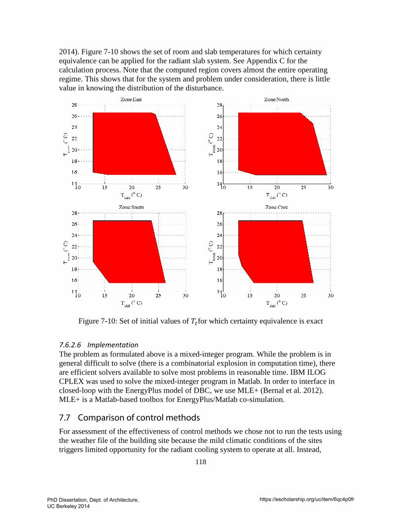
118

2014). Figure 7-10 shows the set of room and slab temperatures for which certainty equivalence can be applied for the radiant slab system. See Appendix C for the calculation process. Note that the computed region covers almost the entire operating regime. This shows that for the system and problem under consideration, there is little value in knowing the distribution of the disturbance.

Figure 7-10: Set of initial values of 𝑇𝑡for which certainty equivalence is exact

7.6.2.6 Implementation The problem as formulated above is a mixed-integer program. While the problem is in general difficult to solve (there is a combinatorial explosion in computation time), there are efficient solvers available to solve most problems in reasonable time. IBM ILOG CPLEX was used to solve the mixed-integer program in Matlab. In order to interface in closed-loop with the EnergyPlus model of DBC, we use MLE+ (Bernal et al. 2012). MLE+ is a Matlab-based toolbox for EnergyPlus/Matlab co-simulation.

7.7 Comparison of control methods For assessment of the effectiveness of control methods we chose not to run the tests using the weather file of the building site because the mild climatic conditions of the sites triggers limited opportunity for the radiant cooling system to operate at all. Instead,



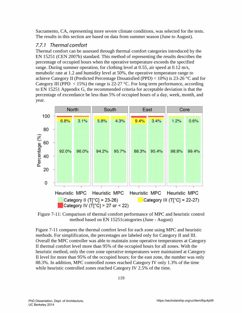
119

Sacramento, CA, representing more severe climate conditions, was selected for the tests. The results in this section are based on data from summer season (June to August).

7.7.1 Thermal comfort Thermal comfort can be assessed through thermal comfort categories introduced by the EN 15251 (CEN 2007b) standard. This method of representing the results describes the percentage of occupied hours when the operative temperature exceeds the specified range. During summer operation, for clothing level at 0.55, air speed at 0.12 m/s, metabolic rate at 1.2 and humidity level at 50%, the operative temperature range to achieve Category II (Predicted Percentage Dissatisfied (PPD) < 10%) is 23-26 °C and for Category III (PPD < 15%) the range is 22-27 °C. For long term performance, according to EN 15251 Appendix G, the recommended criteria for acceptable deviation is that the percentage of exceedance be less than 5% of occupied hours of a day, week, month, and year.

Figure 7-11: Comparison of thermal comfort performance of MPC and heuristic control

method based on EN 15251catogories (June - August)

Figure 7-11 compares the thermal comfort level for each zone using MPC and heuristic methods. For simplification, the percentages are labeled only for Category II and III. Overall the MPC controller was able to maintain zone operative temperatures at Category II thermal comfort level more than 95% of the occupied hours for all zones. With the heuristic method, only the core zone operative temperatures were maintained at Category II level for more than 95% of the occupied hours; for the east zone, the number was only 88.3%. In addition, MPC controlled zones reached Category IV only 1.3% of the time while heuristic controlled zones reached Category IV 2.5% of the time.



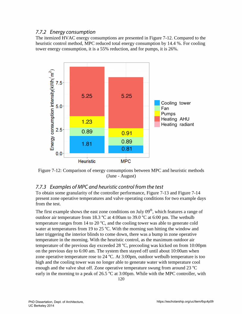
120

7.7.2 Energy consumption The itemized HVAC energy consumptions are presented in Figure 7-12. Compared to the heuristic control method, MPC reduced total energy consumption by 14.4 %. For cooling tower energy consumption, it is a 55% reduction, and for pumps, it is 26%.

Figure 7-12: Comparison of energy consumptions between MPC and heuristic methods

(June - August)

7.7.3 Examples of MPC and heuristic control from the test To obtain some granularity of the controller performance, Figure 7-13 and Figure 7-14 present zone operative temperatures and valve operating conditions for two example days from the test.

The first example shows the east zone conditions on July 09th, which features a range of outdoor air temperature from 18.3 °C at 4:00am to 39.0 °C at 6:00 pm. The wetbulb temperature ranges from 14 to 20 °C, and the cooling tower was able to generate cold water at temperatures from 19 to 25 °C. With the morning sun hitting the window and later triggering the interior blinds to come down, there was a bump in zone operative temperature in the morning. With the heuristic control, as the maximum outdoor air temperature of the previous day exceeded 28 °C, precooling was kicked on from 10:00pm on the previous day to 6:00 am. The system then stayed off until about 10:00am when zone operative temperature rose to 24 °C. At 3:00pm, outdoor wetbulb temperature is too high and the cooling tower was no longer able to generate water with temperature cool enough and the valve shut off. Zone operative temperature swung from around 23 °C early in the morning to a peak of 26.5 °C at 3:00pm. While with the MPC controller, with



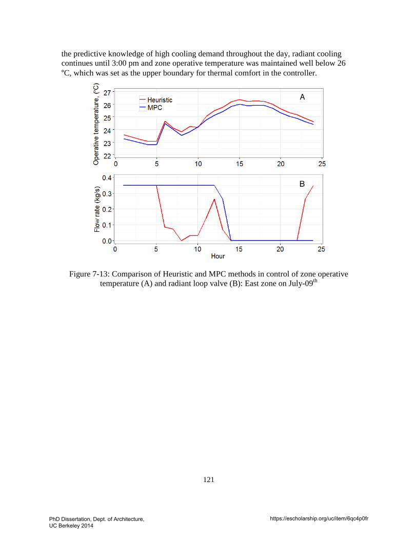
121

the predictive knowledge of high cooling demand throughout the day, radiant cooling continues until 3:00 pm and zone operative temperature was maintained well below 26 °C, which was set as the upper boundary for thermal comfort in the controller.

Figure 7-13: Comparison of Heuristic and MPC methods in control of zone operative temperature (A) and radiant loop valve (B): East zone on July-09th



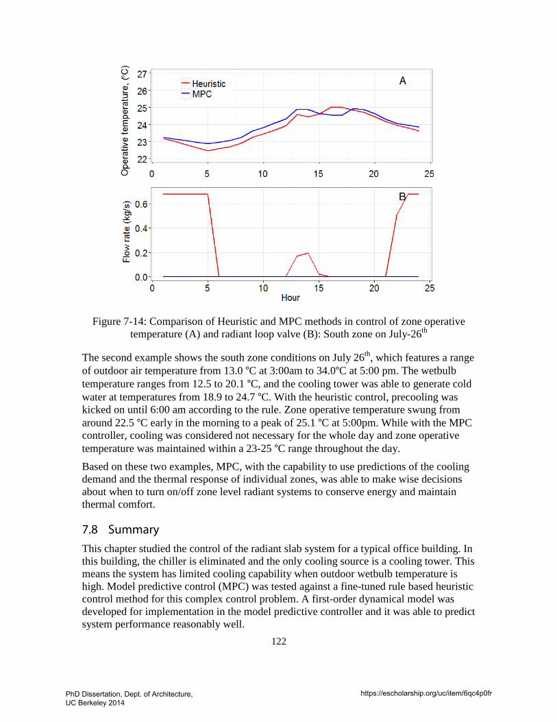
122

Figure 7-14: Comparison of Heuristic and MPC methods in control of zone operative temperature (A) and radiant loop valve (B): South zone on July-26th

The second example shows the south zone conditions on July 26th, which features a range of outdoor air temperature from 13.0 °C at 3:00am to 34.0°C at 5:00 pm. The wetbulb temperature ranges from 12.5 to 20.1 °C, and the cooling tower was able to generate cold water at temperatures from 18.9 to 24.7 °C. With the heuristic control, precooling was kicked on until 6:00 am according to the rule. Zone operative temperature swung from around 22.5 °C early in the morning to a peak of 25.1 °C at 5:00pm. While with the MPC controller, cooling was considered not necessary for the whole day and zone operative temperature was maintained within a 23-25 °C range throughout the day.

Based on these two examples, MPC, with the capability to use predictions of the cooling demand and the thermal response of individual zones, was able to make wise decisions about when to turn on/off zone level radiant systems to conserve energy and maintain thermal comfort.

7.8 Summary This chapter studied the control of the radiant slab system for a typical office building. In this building, the chiller is eliminated and the only cooling source is a cooling tower. This means the system has limited cooling capability when outdoor wetbulb temperature is high. Model predictive control (MPC) was tested against a fine-tuned rule based heuristic control method for this complex control problem. A first-order dynamical model was developed for implementation in the model predictive controller and it was able to predict system performance reasonably well.



123

The test was conducted for a summer season in a dry and hot climate and the MPC controller using the first-order system model was able to maintain zone operative temperatures at EN 15251Category II thermal comfort level more than 95% of the occupied hours for all zones. With the heuristic method, only the core zone operative temperatures were maintained at category II level for more than 95% of the occupied hour; for the east zone, the number was only 88.3%. Compared to the heuristic method, MPC reduced the cooling tower energy consumption by 55% and pumping power consumption by 25%.



124

8 CONCLUSIONS

The building sector consumed 41% of all primary energy produced in the United States, and was responsible for nearly half of U.S. CO2 emissions. Water-based radiant cooling/heating systems are gaining popularity as an energy efficient approach for conditioning buildings. Based on a recent (2012) report by the New Building Institute (NBI), when HVAC systems are used, about half of the zero net energy (ZNE) buildings report using a radiant cooling/heating system, often in conjunction with ground source heat pumps. Radiant systems, however, differ from air systems in terms of the main heat transfer mechanism used to remove heat from a space and their control characteristics when responding to changes in control signals and room thermal conditions. This dissertation investigates three design and control issues that are fundamental to the development of accurate design/modeling tools, relevant performance testing methods, and ultimately the realization of the potential energy benefits of radiant systems.

8.1 Cooling load analysis Cooling load calculations are a crucial step in designing any HVAC system .The main question raised in the dissertation is whether the cooling load for a radiant system is the same as for air systems, and consequently, whether current cooling load analysis and modeling methods, which are developed with an implicit assumption that air systems are used for conditioning space, can be used for radiant systems.

Simulations were conducted to investigate the heat transfer dynamics in spaces conditioned by air vs. radiant systems, and the results confirmed that the two systems have significantly different cooling loads:

• For perimeter zones that were subjected to building envelope heat gain, percentage difference of peak cooling load between the two systems ranged from 12% to 25% for the radiant ceiling panel systems (RCP), 16% to 27% for the lightweight embedded systems (ESS), and 31% to 35% for the thermally active building systems (TABS).

• For interior zones with internal load, the peak cooling rate differences ranged from 7% to 27% at the surface level depending on radiant fraction of the internal load. The higher the radiant fraction, the higher the difference. This implies that higher radiant fraction in heat gain produces larger differences in peak cooling rates between the two systems at the surface level.

• For perimeter zones and atrium where direct solar heat gain constitutes a large portion of the cooling load, the peak cooling load difference is pronounced. When exterior shading was not installed, RCP ceiling surface peak cooling rate is 36% higher than the air system, and for ESS ceiling system it is 35%, and 49% for TABS ceiling systems. Exterior shading reduced the direct solar impact, but the surface peak cooling rates were still 24-33% higher for the ceiling system.



125

• When the floor was used as the radiant cooling surface and when it was illuminated by direct solar, surface peak cooling load increased dramatically compared to the ceiling cases. The ESS surface peak cooling rate was 69% higher and for TABS, 85% higher.

Laboratory testing results also confirmed that there are significant differences (18 – 21%) between air and radiant system peak cooling load for the case with internal load. The experiments showed that radiant systems remove heat faster than air systems. In fact, 75-82% of total heat gain was removed by radiant system during the period when the heater was on, while for air system, 61-63% were removed. The differences were caused by the amount of energy stored in non-active mass. The temperatures of non-active mass (concrete blocks in this paper) are at the peak approximately 1˚C lower for the radiant cases, meaning less energy storage for the radiant cases.

From a heat transfer perspective, the differences are due to the following: 1) chilled surfaces directly remove part of radiant heat gains from a zone, thereby bypassing the time-delay effect caused by the interaction of radiant heat gain with non-active thermal mass in air systems; and 2) only part of the convective heat gain becomes instantaneous cooling load, the remainder partly contributes to increased air temperature and partly is stored in the building mass and removed by the radiant surface as surface cooling load.

The study also concluded that there are important limitations in the definition of cooling load for a mixing air system described in Chapter 18 of ASHRAE Handbook of Fundamentals when applied to radiant systems: 1) radiant systems remove heat at the cold surface, i.e. the heat transfer balance for load analysis should be conducted at the radiant surface, instead of the air volume, as is in the case for air systems; 2) operative temperature, instead of air temperature, is a better reference for calculating the cooling load for radiant system; and 3) for radiant panels and lightweight embedded systems, peak surface cooling load shall be used for dimensioning total required cooling surface area, and peak hydronic cooling load shall be used for sizing associated cooling equipment. For thermally massive systems, control strategy should be considered.

Due to the obvious mismatch between how radiant heat transfer is handled in traditional cooling load calculation methods compared to its central role in radiant cooling systems, this dissertation recommends improvements for current cooling load analysis methods and provides guidance for selection of load calculation and modeling tools:

• The current cooling load calculation method based on Heat Balance procedure need to be modified to properly consider the cooling load definition for radiant system.

• Sensible cooling load calculations for radiant systems should utilize dynamic energy simulation programs or design tools based on a fundamental heat balance approach that properly takes into account how heat gains are removed from a zone by an actively cooled surface. Some examples of whole building simulation tools with such capability are EnergyPlus, IES-VE, TRNSYS, IDA-ICE, and ESP-r. I recommend to model radiant system utilizing those tools for load prediction and system sizing.



126

• Simplified cooling load calculation methods, such as RTS or weighting factor method, may lead to incorrect results for radiant systems. These algorithms are widely implemented in building thermal simulation or load calculation tools, including HAP (TF), TRANE TRACE (RTS), BLAST, and DOE-2 (TF) based tools such as eQUEST, Energy-pro, Green Building Studio and VisualDOE.

• The above recommendations also directly apply to the selection of whole building energy simulation software for evaluation of system energy and thermal comfort performance.

This finding has important implications for the proper design and sizing of radiant systems along with the required reduced-sized air distribution system (radiant systems provide only sensible cooling, and they are typically configured as a hybrid with an air system, which is used for ventilation, dehumidification and supplemental cooling if needed). More broadly, the findings of the research into this question can be applied to all space conditioning systems that involve radiation heat transfer, such as underfloor air distribution systems (UFAD) and displacement ventilation, which will create non-uniform surface temperatures in the space.

8.2 Radiant system capacity Cooling capacity estimation is another critical step in a design project. Theoretical analysis of the heat transfer process between the space and the radiant cooling surface reveals that the existing radiant cooling capacity estimation methods are insufficient when the system is exposed to solar radiation or large fractions of lighting loads, because only convective and longwave radiation heat transfer are considered in the calculation methods. The simulation results for a total of 864 runs showed that floor surface radiation heat flux is, in median, 1.44 and 1.2 times higher than the values calculated with ISO 11855 and ASHRAE methods, respectively. The difference is caused by absorption of shortwave radiation. The ASHRAE method, which calculates surface radiation and convection heat flux separately, has better predictability than the ISO method, which calculates surface heat flux using a combined heat transfer coefficient.

The simulation results also confirm that ISO 11855 cooling capacity estimation method does not apply to cases when there is solar load (the CVRMSE was 54.1 %). When interior blinds are installed to block solar gain, ISO 11855 cooling capacity estimation methods can well predict the system performance. When there is no shading system, the system capacity can increase up to 130-140 W/m2 at a standard system temperature difference of 10 °C.

To improve the predictability of the cooling capacity estimation methods for cases with direct solar heat gain, a new equation is proposed to estimate system capacity enhancement due to direct solar absorption. The new model calculates the enhanced capacity as a function of window’s transmitted solar and a mean temperature differences between the hydronic loop and room operative temperature. The new regression model has an adjusted R2

adj = 0.92.



127

This paper also addressed the question regarding sizing of the associated air system in cases when radiant system capacity are enhanced by solar. The new model was used to predict radiant floor system capacity, and when compared with EnergyPlus simulated cooling capacity, the CVRMSE was 22.1 %. The new simplified model enables designers to more accurately size the associated air system and therefore avoid oversizing the air system by a significant amount.

8.3 Control of radiant slab systems For the design of heavyweight radiant slab systems, control strategies have to be taken into account for load analysis and equipment sizing. The dissertation compares the energy and comfort benefits of model-based predictive control (MPC) method with a fine-tuned heuristic control method when applied to a heavyweight embedded surface system.

A calibrated EnergyPlus model of a typical office building in California was used as a testbed for the comparison. The case study building is a LEED platinum office building conditioned by a radiant system using an evaporative cooling source. The EnergyPlus model was validated against field measurement data and the 2012 trending data from the building management system at three levels: 1) radiant slab thermal response; 2) monthly HVAC components’energy consumptions; and 3) zone level hourly and annual thermal comfort conditions (air temperature). The comparison results indicate that the EnergyPlus model does a good job of capturing the HVAC performance and the thermal comfort environment in the building.

A first order dynamic model of a radiant slab system was developed for implementation in model predictive controllers. Their performance was compared with fine-tuned rule based control method that was modified based on existing control sequence implemented in the building. The test was conducted for a summer season in a dry and hot climate, and the MPC controller was able to maintain zone operative temperatures at EN 15251Category II thermal comfort level more than 95% of the occupied hours for all zones. With the heuristic method, only the core zone operative temperatures were maintained at Category II level for more than 95% of the occupied hours; for the east zone, the number was only 88.3%. Compared to the heuristic method, MPC reduced the cooling tower energy consumption by 55% and pumping power consumption by 26%.

In summary, the dissertation work have: (1) provided clear evidence that the fundamental heat transfer mechanisms differ between radiant and air systems and these findings have important implications for the development of accurate and reliable design and energy simulation tools; (2) developed practical design methods and guidance to aid practicing engineers who are designing radiant systems; and (3) outlined future research and design tool needs to advance the state-of-knowledge and design and operating guidelines for radiant systems.



128

9 REFERENCE

Abellon, D. (2011). "Blueprint for America's energy future-Radiant slab system highlights first-of-its-kind green office building." PME.

Achermann, M. and G. Zweifel (2003). RADTEST – Radiant Heating and Cooling Test Cases., IEA Task 22, Subtask C, International Energy Agency.

Andrés-Chicote, M., A. Tejero-Gonzalez, E. Velasco-Gomez and F. J. Rey-Martinez (2012). "Experimental study on the cooling capacity of a radiant cooled ceiling system." Energy and Buildings 54: 207-214.

ANSI/ASHRAE (2010). "ANSI/ASHRAE 62.1-2010: Ventilation for acceptable indoor air quality." American Society of Heating, Refrigerating and Air-Conditioning Engineers, Atlanta(Journal Article).

Antonopoulos, K. (1992). "Analytical and numerical heat transfer in cooling panels." International Journal of Heat and Mass Transfer 35(11): 2777-2782.

Antonopoulos, K. and F. Democritou (1993). "Periodic steady-state heat transfer in cooling panels." International Journal of Heat and Mass Transfer 14(1): 94-100.

Antonopoulos, K. and C. Tzivanidis (1997a). "Numerical solution of unsteady three-dimensional heat transfer during space cooling using ceiling-embedded piping." Energy 22(1): 59-67.

Antonopoulos, K. A., M. Vrachopoulos and C. Tzivanidis (1997b). "Experimental and theoretical studies of space cooling using ceiling-embedded piping." Applied Thermal Engineering 17(4): 351-367.

APS (2008). Energy Future: Thinking efficiency-How American can look within to achieve energy security and reduce global warming, American Physical Society (APS).

Arbab, M. and J. J. Finley (2010). "Glass in Architecture." International Journal of Applied Glass Science 1(1): 118-129.

ASHRAE (2002). ASHRAE Guideline 14-2002: Measurement of Energy and Demand Savings. Altanta,GA, American Society of Heating, Refrigerating and Air Conditioning Engineers .Inc.

ASHRAE (2007). ANSI/ASHRAE Standard 140-2007: Standard Method of Test Fort the Evaluation of Building Energy Analysis Computer Program. Atlanta, GA, American Society of Heating, Refrigerating and Air Conditioning Engineers .Inc.



129

ASHRAE (2009). ANSI/ASHRAE 138-2009: Method of Testing for Rating Ceiling Panels for Sensible Heating and Cooling. Altanta,GA, American Society of Heating, Refrigerating and Air Conditioning Engineers .Inc.

ASHRAE (2010). ANSI/ASHRAE 55-2010: Thermal environmental conditions for human occupancy. 55.

ASHRAE (2012a). Chapter 6: Panel heating and cooling. ASHRAE Handbook: HVAC Systems and Equipment. Altanta,GA, American Society of Heating, Refrigerating and Air Conditioning Engineers Inc.

ASHRAE (2012b). Chapter 31: Boilers. ASHRAE Handbook: HVAC Systems and Equipment. Altanta,GA, American Society of Heating, Refrigerating and Air Conditioning Engineers Inc.

ASHRAE (2012c). Chapter 37: Compressors. ASHRAE Handbook: HVAC Systems and Equipment. Altanta,GA, American Society of Heating, Refrigerating and Air Conditioning Engineers Inc.

ASHRAE (2013a). Chapter 18: Nonresidential cooling and heating load calculations. ASHRAE Handbook of Fundamentals. Atlanta, GA, American Society of Heating, Refrigerating and Air-Conditioning Engineers.

ASHRAE (2013b). Chapter 19: Energy estimating and modeling methods. ASHRAE Handbook of Fundamentals. Atlanta, GA.

Athienitis, A. and Y. Chen (2000). "The effect of solar radiation on dynamic thermal performance of floor heating systems." Solar Energy 69(3): 229-237.

Awbi, H. and A. Hatton (1999). "Natural convection from heated room surfaces." Energy and Buildings 30(3): 233-244.

Babiak, J. (2007). Low temperature heating and high temperature cooling_Thermally activated building system. Ph.D, Technical University of Denmark.

Babiak, J., B. Olesen and D. Petras (2007). REHVA guidbook NO. 7: Low temperature heating and high temperature cooling Brussels, Belgium, Federation of European Heating and Air-Conditioning Associations.

Bauman, F., T. Webster, D. Dickerhoff, S. Schiavon, J. Feng and C. Basu (2011). Case study report: David Brower Center. Internal report, Center for the Built Environment, University of California, Berkeley.

Benton, C., F. Bauman and M. Fountain (1990). "A field measurement system for the study of thermal comfort." ASHRAE Transactions 96(1).



130

Bernal, W., M. Behl, T. X. Nghiem and R. Mangharam (2012). MLE+: a tool for integrated design and deployment of energy efficient building controls. Proceedings of the Fourth ACM Workshop on Embedded Sensing Systems for Energy-Efficiency in Buildings, ACM.

Borrelli, F., A. Bemporad and M. Morari (2010). Constrained optimal control and predictive control for linear and hybrid systems, University of California , Berkeley.

Borresen, B. (1994). Floor heating and cooling of an atrium. 16th Internationaler Velta-KongreB Arlberg/St. Christoph. .

Causone, F., S. P. Corgnati, M. Filippi and B. W. Olesen (2009). "Experimental evaluation of heat transfer coefficients between radiant ceiling and room." Energy and Buildings 41(6): 622-628.

Causone, F., S. P. Corgnati, M. Filippi and B. W. Olesen (2010). "Solar radiation and cooling load calculation for radiant systems: Definition and evaluation of the Direct Solar Load." Energy and Buildings 42(3): 305-314.

CEN (2003). EN 12831-2003, Heating systems in buildings-Method for calculation of the design heat load. Brussels, Belgium, European Committee for Standardization.

CEN (2004). EN 14240-2004, Ventilation for Buildings-Chilled Ceilings Testing and Rating. Brussels, Belgium, European Committee for Standardization.

CEN (2007a). EN 15243-2007, Ventilation for buildings-Calculation of room temperature and of load and energy for buildings with room conditioning systems. Brussels, Belgium, European Committee for Standardization.

CEN (2007b). EN 15251-2007, Criteria for the indoor environment including thermal, indoor air quality, light and noise. Brussels, Belgium, European Committee for Standardization.

CEN (2007c). EN 15255-2007, Thermal performance of buildings – Sensible room cooling load calculation – General criteria and validation procedures. Brussels, Belgium, European Committee for Standardization.

CEN (2008). EN 15377-2008, Heating systems in buildings. Design of embedded water based surface heating and cooling systems. Brussels, Belgium, European Committee for Standardization.

CEN (2011). EN 1264-2001, Water based surface embedded heating and cooling systems. Brussels, Belgium, European Committee for Standardization.

CEN (2013). EN 14037-2013, Free hanging heating and cooling surfaces for water with a temperature below 120 C. Brussels, Belgium, European Committee for Standardization.



131

Chantrasrisalai, C., V. Ghatti, D. E. Fisher and D. G. Scheatzle (2005). "Experimental Validation of the EnergyPius Low-Temperature Radiant Simulation." ASHRAE Transactions 109(2).

Chapman, K. S., J. Rutler and R. D. Watson (2000). "Impact of heating systems and wall surface tempeartures on room operative temperature fields." ASHRAE Transaction 106(1): 506-514.

Chen, Q. (1990). "Comfort and energy consumption analysis in buildings with radiant panels." Energy and Buildings 14(4): 287-297.

Cholewa, T., M. Rosinski, Z. Spik, M. R. Dudziiska and A. Siuta-Olcha (2013). "On the heat transfer coefficients between heated/cooled radiant floor and room." Energy and Buildings(66): 599-606.

Chuang, F., C. Danielson and F. Borrelli (2014). Optimality of certainty equivalence in expected value problems for uncertain linear systems. Available at http://arxiv.org/abs/1404.0413.

Clements-Croome, D. (2006). Creating the productive workplace. New York, Taylor & Francis.

Coffey, B. (2008). A development and testing framework for simulation-based supervisory control with application to optimal zone temperature ramping demand response using a modified genetic algorithm, Concordia University.

Coffey, B. (2011). Using Building Simulation and Optimization to Calculate Lookup Tables for Control. Ph.D, University of California at Berkeley.

Conroy, C. L. and S. A. Mumma (2001). "Ceiling radiant cooling panels as a viable distributed parallel sensible cooling technology integrated with dedicated outdoor air systems." ASHRAE Transactions 107(1): 578-588.

Corbin, C. D., G. P. Henze and P. May-Ostendorp (2012). "A model predictive control optimization environment for real-time commercial building application." Journal of Building Performance Simulation.

Corgnati, S. P. (2002). Heat flows and air distribution in rooms cooled by radiant panels. Ph.D., Politecnico de Torino.

Creyts, J. C. (2007). Reducing US greenhouse gas emissions: How much at what cost?, Mckinsey&Company.

Diaz, N. and C. Cuevas (2011). "Experimental study of the energy and thermal comfort performance of chilled ceiling panel." HVAC&R RESEARCH 17(3).

DOE (2011). "EnergyPlus Engineering Reference."



http://arxiv.org/abs/1404.0413

132

DOE (2012). " EnergyPlus Energy Simulation Software." 2012.

DOE, (2011). EnergyPlus Engineering Reference.

Doebber, I., M. Moore and M. Deru (2010). "Radiant slab cooling for retail." ASHRAE Journal 52(12).

EIA (2012). Annual Energy Review 2011. Washington DC, Energy Information Administration, Department of Energy.

EN/ISO (1993). "EN/ISO-13005:1993, Guide to the Expression of Uncertainty in Measurement."

Fabrizio, E., S. P. Corgnati, F. Causone and M. Filippi (2011). "Numerical comparison between energy and comfort performances of radiant heating and cooling systems versus air systems." HVAC&R RESEARCH 18(4): 692-708.

Feng, J., F. Bauman and S. Stefano (2014). Critical Review of Water Based Radiant Cooling System Design Methods. Proceedings of the 13th International Conference on Indoor Air Quality and Climate, Indoor Air 2014 Hong Kong, China, http://128.48.120.176/uc/item/2s00x6ns.

Feng, J., S. Schiavon and F. Bauman (2013). Impact of Solar Heat Gain on Radiant Floor Cooling System Design. Proceedings of the 11th REHVA World Congress-CLIMA 2013. Prague, Czech Republic

Feustel, H. E. and C. Stetiu (1995). "Hydronic radiant cooling-A preliminary assessment." Energy and Buildings 22(3): 193-205.

Fischer, D. (2006). Final Report for ASHRAE RP-1282: Lighting heat gain distribution in buildings, Okalahoma State University.

Fisher, D. E. (1995). "An experimental investigation of mixed convection heat transfer in a rectangular enclosure." PhD dissertation.

Fisk, W. J. (2000). "Health and productivity gains from better indoor environments and their relationship with building energy efficiency." Annual Review of Energy and the Environment 25(1): 537-566.

Florides, G. A., S. A. Tassou, S. A. Kalogirou and L. C. Wrobel (2002). "Review of solar and low energy cooling technologies for buildings." Renewable and Sustainable Energy Reviews 6(6): 557-572.

Fonseca, N. (2011). "Experimental analysis and modeling of hydronic radiant ceiling panels using transient-state analysis." International Journal of Refrigeration 34(4): 958-967.

Fort, K. TRNSYS TYPE 360: Floor heating and hypocaust.



http://128.48.120.176/uc/item/2s00x6ns

133

Gao, M., F.-z. Sun, K. Wang, Y.-t. Shi and Y.-b. Zhao (2008). "Experimental research of heat transfer performance on natural draft counter flow wet cooling tower under cross-wind conditions." International Journal of Thermal Sciences 47(7): 935-941.

Gayeski, N. T. (2010). Predictive pre-cooling control for low lift radiant cooling using building thermal mass. PhD, Massachusettes Institute of Technology.

Ghatti, V. (2003). "Experimental Validation of the EnergyPius Low-Temperature Radiant Simulation." Transactions 109(2): 614-623.

Glicksman, L. R. (2008). "Energy efficiency in the built environment." Physics Today 61(7): 35.

Gwerder, M., B. Lehmann, J. Tödtli, V. Dorer and F. Renggli (2008). "Control of thermally-activated building systems (TABS)." Applied Energy 85(7): 565-581.

Gwerder, M., J. Todtli, B. Lehmann, V. Dorer, W. Guntensperger and F. Renggli (2009). "Control of thermally activated building systems (TABS) in intermittent operation with pulse width modulation." Applied Energy 86(9): 1606-1616.

Hang, Y., M. Qu and F. Zhao (2011). "Economical and environmental assessment of an optimized solar cooling system for a medium-sized benchmark office building in Los Angeles, California." Renewable Energy 36(2): 648-658.

Hedgepeth, L. and C. Sepsy (1972). "A thermodynamic simulation of a radiant panel heating system." ASHRAE Transactions 78(2): 50-60.

Henze, G. and M. Krarti (2005). Predictive optimal control of active and passive building thermal storage inventory: final report.

Henze, G. and C. Neumann (2011). Building simulation in building automation systems. Building performance simulation for design and operation. J. Hensen and R. Lamberts, Spon Press.

Hirsch, A., S. Pless, R. Guglielmetti and P. Torcellini (2011). The Role of Modeling When Designing for Absolute Energy Use Intensity Requirements in a Design-Build Framework, National Renewable Energy Laboratory.

Hosni, M. H. and B. T. Beck (2009). ASHRAE RP1482 Final Report: Update to measurement of office equipment heat gain data, Kansas State University.

Howell, J. R., R. Siegel and M. P. Menguc (2011). Thermal radiation heat transfer, CRC Press.

Howell, R. (1987). Final Report for ASHRAE RP-394: A study to determine methods for designing radiant heating and cooling systems, Department of Mechanical and Aerospace Engineering, Univeristy of Missouri-Rolla.



134

Hoyt, T., K. H. Lee, H. Zhang, E. Arens and T. Webster (2009). Energy savings from extended air temperature setpoints and reductions in room air mixing. International Conference on Environmental Ergonomics, Boston. http://dx.doi.org/10.1016/j.enbuild.2008.05.001

Hu, J. and P. Karava (2014). "Model predictive control strategies for buildings with mixed-mode cooling." Building and Environment 71(0): 233-244.

Imanari, T., T. Omori and K. Bogaki (1999). "Thermal comfort and energy consumption of the radiant ceiling panel system: Comparison with the conventional all-air system." Energy and Buildings 30(2): 167-175.

Incropera, F. P., A. S. Lavine and D. P. DeWitt (2011). Fundamentals of heat and mass transfer, John Wiley & Sons Incorporated.

ISO (1998). ISO-7726: Ergonomics of the thermal environment-Instruments for measuring physical quantities.

ISO (2012a). ISO 11855-2-2012, Building environment design -- Design, dimensioning, installation and control of embedded radiant heating and cooling systems -- Part 2: Determination of the design heating and cooling capacity, International Organization for Standardization.

ISO (2012b). ISO 11855-4-2012, Building environment design -- Design, dimensioning, installation and control of embedded radiant heating and cooling systems -- Part 4: Dimensioning and calculation of the dynamic heating and cooling capacity of Thermo Active Building Systems (TABS), International Organization for Standardization.

ISO (2012c). ISO-11855: 2012, Building Environment Design—Design,Dimensioning, Installation and Control of Embedded Radiant Heating and Cooling Systems, International Organization for Standardization.

JCGM (2008). JCGM 100: Evaluation of measurement data - Guide to the expression of uncertainty in measurements.

Jeong, J. (2003). "Ceiling radiant cooling panel capacity enhanced by mixed convection in mechanically ventilated spaces." Applied Thermal Engineering 23(18): 2293-2306.

Jeong, J.-W. and S. A. Mumma (2003). "Impact of mixed convection on ceiling radiant cooling panel capacity." HVAC&R Research 9(3): 251-257.

Jeong, J.-W. and S. A. Mumma (2004). "Simplified cooling capacity estimation model for top insulated metal ceiling radiant cooling panels." Applied Thermal Engineering 24(14): 2055-2072.



http://dx.doi.org/10.1016/j.enbuild.2008.05.001

135

Johes, C., G. Crall, C. Sepsy and J. Johns (1975). "Simulation and verification of a hydronic sub-system with radiant panels." ASHRAE Transactions 81(1): 457-462.

Karadag, R. (2009). "New approach relevant to total heat transfer coefficient including the effect of radiation and convection at the ceiling in a cooled ceiling room." Applied thermal engineering 29(8‚Äì9): 1561-1565.

Kilkis, B. (1993). Enhancement of heat pump performance by using radiant heating and cooling panels. Heat Pumps for Energy Efficiency and Environmental Progress. J. Bosma. Oxford, Elsevier: 269-277.

Kilkis, B. I., M. Eltez and S. S. Sager (1995). "3851 A Simplified Model for the Design of Radiant In-Slab Heating Panels." ASHRAE Transactions 101(1): 210-216.

Kilkis, I. and M. Sapci (1995). "Computer-aided design of radiant subfloor heating systems." ASHRAE Transactions 101(1): 1214-1220.

Kilkis, I. B. and M. Coley (1995). "Development of a complete design software for hydronic floor heating of buildings." ASHRAE Transactions 101(1): 1201-1213.

Koschenz, M. and V. Dorer (1999). "Interaction of an air system with concrete core conditioning." Energy and Buildings 30(2): 139-145.

Koschenz, M. and B. Lehmann (2000). Thermoaktive Bauteilsysteme. Switzerland, EMPA, Zentrum fu r Energie und Nachhaltigkeit.

Kuehn, T., J. Ramsey and J. Threlkeld (1998). Thermal Environmental Engineering Prentice-Hall,Inc.

Kuwabara, B., T. Auer, T. Akerstream and G. Kylm (2011). "Harnessing climate." High Performance Buildings Fall.

Leach, M., C. Lobato, A. Hirsch, S. Pless and P. Torcellini (2010). Technical Support Document: Strategies for 50% Energy Savings in Large Office Buildings, Pacific Northwest National Laboratory.

Lehmann, B., V. Dorer, M. Gwerder, F. Renggli and J. Todtli (2011). "Thermally activated building systems (TABS): Energy efficiency as a function of control strategy, hydronic circuit topology and (cold) generation system." Applied Energy 88(1): 180-191.

Lehmann, B., V. Dorer and M. Koschenz (2007). "Application range of thermally activated building systems tabs." Energy and Buildings 39(5): 593-598.

Lindstrom, P. C., D. E. Fisher and C. O. Pedersen (1998). "Impact of Surface Characteristics on Radiant Panel Output." ASHRAE Transactions 104(1): 1079-1089.



136

Lu, C. (2013) "CTF/PRF Generator.", from: http://www.hvac.okstate.edu/resources.html.

Ma, Y., A. Kelman, A. Daly and F. Borrelli (2012). "Predictive Control for Energy Efficient Buildings with Thermal Storage: Modeling, Stimulation, and Experiments." Control Systems, IEEE 32(1): 44-64.

May-Ostendorp, P., G. P. Henze, C. D. Corbin, B. Rajagopalan and C. Felsmann (2011). "Model-predictive control of mixed-mode buildings with rule extraction." Building and Environment 46(2): 428-437.

May-Ostendorp, P. T., G. P. Henze, B. Rajagopalan and D. Kalz (2013). "Experimental investigation of model predictive control-based rules for a radiantly cooled office." HVAC&R Research 19(5): 602-615.

McDonell, G. (2012). Email communication.

Mumma, S. A. (2001). "Designing dedicated outdoor air systems." ASHRAE Journal 43(5): 28-32.

Nadine, M. (2007). "Owner Is Radiant About Lobby’s Radiant Cooling." 2012, from http://enr.construction.com/news/buildings/archives/070926b.asp.

Nall, D. (2013). "Thermally active floors." ASHRAE Journal 36(1-3).

Nall, D. and R. Ellington (2001). Design and operation of radiant heating/cooling systems for non-residental buildings. Cooling Frontiers, Conference of the Arizona State University School of Architecture, Tempe, AZ.

Nghiem, T. X. (2012). Green scheduling of control systems PhD dissertation, University of California.

Niu, J. (1997). "Cooling load dynamics of rooms with cooled ceilings." Building Services Engineering Research and Technology 18(4): 201-207.

Novoselac, A., B. J. Burley and J. Srebric (2006). "New Convection Correlations for Cooled Ceiling Panels in Room with Mixed and Stratified Airflow." HVAC&R Research 12(2): 279-294.

Odyjas, A. and A. Gorka (2013). "Simulations of floor cooling system capacity." Applied thermal engineering 51: 84-90.

Oldewurtel, F., A. Parisio, C. N. Jones, D. Gyalistras, M. Gwerder, V. Stauch, B. Lehmann and M. Morari (2012). "Use of model predictive control and weather forecasts for energy efficient building climate control." Energy and Buildings 45: 15-27.



http://www.hvac.okstate.edu/resources.html

http://enr.construction.com/news/buildings/archives/070926b.asp

137

Olesen, B. (1997a). "Possibilities and Limitations of Radiant Cooling." ASHRAE Transactions 103(1): 7.

Olesen, B. (2007b). New European standards for design, dimensioning and testing embedded radiant heating and cooling systems. Proceedings of Clima 2007.

Olesen, B. (2001). "Radiant Floor Heating in Theory and Practice." Ashrae Journal 43(7): 19-24.

Olesen, B. (2008). "Radiant floor cooling systems." ASHRAE Journal 50(9): 16-22.

Olesen, B., K. Sommer and D. Duchting (2002). "Control of Slab Heating and Cooling Systems Studied by Dynamic Computer Simulations." ASHRAE Transaction 108(2): 10.

Olesen, B. W., F. Bonnefoi, E. Michel and M. d. Carli (2000). "Heat exchange coefficient between floor surface and space by floor cooling -- Theory or a question of definition." ASHRAE Transactions 106(1): 929.

Olesen, B. W., M. de Carli, M. Scarpa and M. Koschenz (2006). "Dynamic Evaluation of the Cooling Capacity of Thermo-Active Building Systems." ASHRAE Transaction 112(1): 350-357.

Pedersen, C. O., D. E. Fisher and R. J. Liesen (1997). "Development of a heat balance procedure for calculating cooling loads." ASHRAE Transactions 103(2): 459-468.

PRICE (2011). Introduction to radiant heating and cooling. Engineer's HVAC Handbook_A comprehensive guide to HVAC fundamentals.

Q. Chen and J. v. d. Kooi (1988). "ACCURACY—a computer program for combined problems of energy analysis, indoor airflow and airquality." ASHRAE Transaction 94(2).

Raftery, P., K. H. Lee, T. Webster and F. Bauman (2011). Analysis of a hybrid UFAD and radiant hydronic slab HVAC system.

Reinhart, C. (2011). Daylight performance predictions. Building performance simulation for design and operation. J. Hensen and R. Lamberts, Spon Press.

Rijksen, D. O., C. J. Wisse and A. W. M. van Schijndel (2010). "Reducing peak requirements for cooling by using thermally activated building systems." Energy and Buildings 42(3): 298-304.

Saelens, D., W. Parys and R. Baetens (2011). "Energy and comfort performance of thermally activated building systems including occupant behavior." Building and Environment 46(4): 835-848.



138

Sakulpipatsin, P., L. C. M. Itard, H. J. van der Kooi, E. C. Boelman and P. G. Luscuere (2010). "An exergy application for analysis of buildings and HVAC systems." Energy and Buildings 42(1): 90-99.

Shell, S. (2013). Architectural implications of radiant systems. Presentation at semiar "Radiant Systems: HVAC Design, Energy Assessment and Architectural Implications", sponsored by Golden Gate ASHRAE Chapter at PG&E.

Simmonds, P., S. Holst, S. Reuss and W. Gaw (1999). "Comfort Conditioning for Large Spaces." ASHRAE Transactions 105(1): 1037-1048.

Simmonds, P., S. Holst, S. Reuss and W. Gaw (2000). "Using radiant cooled floors to condition large spaces and maintain comfort conditions." ASHRAE Transactions 106(1): 695-701.

Simmonds, P., S. Holst, S. Reuss and W. Gaw (2000). "Using radiant cooled floors to condition large spaces and maintain comfort conditions." TRANSACTIONS-AMERICAN SOCIETY OF HEATING REFRIGERATING AND AIR CONDITIONING ENGINEERS 106(1): 695-701.

Simmonds, P., S. Holst, S. Reuss and W. Gaw (2000). "Using radiant cooled floors to condition large spaces and maintain comfort conditions." ASHRAE Transactions 106(1): 695-701.

Simmonds, P., B. Mehlomakulu and T. Ebert (2006). "Radiant cooled floors: Operation and control dependant upon solar radiation." ASHRAE Transactions: 358-367.

Spitler, J. D. (1990). An experimental investigation of air flow and convective heat transfer in enclosures having large ventilative flow rates, University of Illinois.

Spitler, J. D. (2011). Thermal load and energy performace prediction. Building performance simulation for design and operation. J. Hensen and R. Lamberts, Spon Press.

Spitler, J. D., D. E. Fisher and C. O. Pedersen (1997). "The radiant time series cooling load calculation procedure." ASHRAE Transactions 103: 503-518.

Spitler, J. D., F. C. McQuiston and K. Lindsey (1993). "The CLTD/SCL/CLF Cooling Load Calculation Method." ASHRAE Transactions 99(1): 183-192.

Stetiu, C. (1999). "Energy and peak power savings potential of radiant cooling systems in US commercial buildings." Energy and Buildings 30(2): 127-138.

Stetiu, C., H. E. Feustel and F. Winkelmann (1995). Development of a simulation tool to evaluate the performance of radiant cooling ceilings,, LBNL-37300.



139

Strand, R. and K. Baumgartner (2005). "Modeling radiant heating and cooling systems: integration with a whole-building simulation program." Energy and Buildings 37(4): 389-397.

Thornton, B. A., W. Wang, M. D. Lane, M. I. Rosenberg and B. Liu (2009). Technical Support Document: 50% Energy Savings Design Technology Packages for Medium Office Buildings, Pacific Northwest National Laboratory.

Tian, Z. and J. A. Love (2009). "Energy performance optimization of radiant slab cooling using building simulation and field measurements." Energy and Buildings 41(3): 320-330.

Tian, Z., X. Yin, Y. Ding and C. Zhang (2012). "Research on the actual cooling performance of ceiling radiant panel." Energy and Buildings 47(0): 636-642.

Uponor (2010). Uponor indoor climate solution technical guideline: Uponor plaster system for ceiling and wall cooling/heating. Uponor.

Uponor. (2012). "Radiant Cooling Systems." from http://www.uponor-usa.com/Misc/Applications/Radiant-Cooling.aspx.

Uponor. (2012). "Uponor case study." from http://www.uponor.com/en/references.aspx.

Uponor, I. (2011). Radiant heating and cooling system: Complete design assistance manual

Uponor, I. (2013). Radiant cooling design manual.

Weber, T. and G. Johannesson (2005). "An optimized RC-network for thermally activated building components." Building and Environment 40(1): 1-14.

Weber, T., G. Johannesson, M. Koschenz, B. Lehmann and T. Baumgartner (2005). "Validation of a FEM-program (frequency-domain) and a simplified RC-model (time-domain) for thermally activated building component systems (TABS) using measurement data." Energy and Buildings 37(7): 707-724.

Wei, Z. and R. Zmeureanu (2009). "Exergy analysis of variable air volume systems for an office building." Energy Conversion and Management 50(2): 387-392.

Weitzmann, P. (2004). Modelling building integrated heating and cooling systems. PhD, Danmark Technisk Universite.

Whitney, D. and J. Kipnis (1993). Philip Johnson: The Glass House, Pantheon.

Zhang, L., X.-H. Liu and Y. Jiang (2012). "Simplified calculation for cooling/heating capacity, surface temperature distribution of radiant floor." Energy and Buildings 55(0): 397-404.



http://www.uponor-usa.com/Misc/Applications/Radiant-Cooling.aspx

http://www.uponor-usa.com/Misc/Applications/Radiant-Cooling.aspx

http://www.uponor.com/en/references.aspx

140

Zhao, K., X.-H. Liu and Y. Jiang (2013). "Application of radiant floor cooling in a large open space building with high-intensity solar radiation." Energy and Buildings 66.



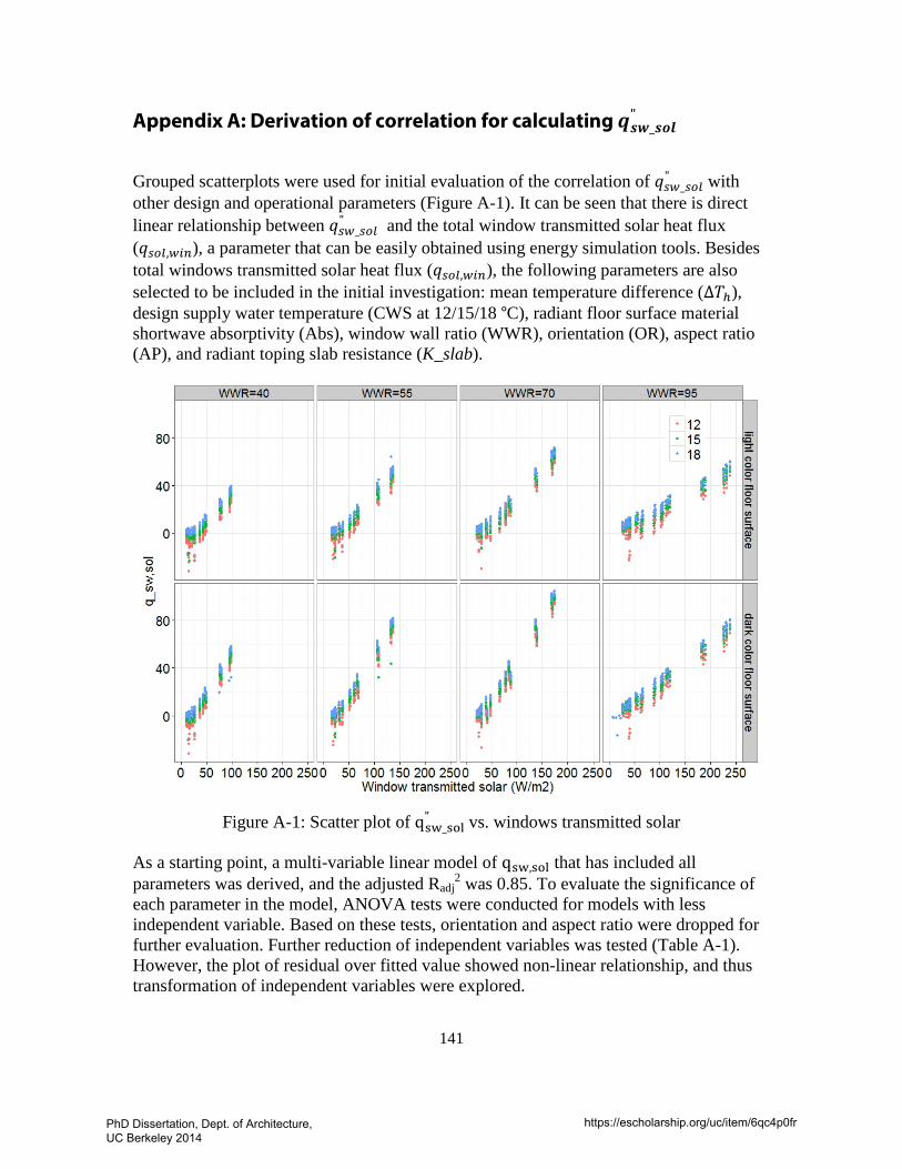
141

Appendix A: Derivation of correlation for calculating 𝒒𝒔𝒘_𝒔𝒐𝒍"

Grouped scatterplots were used for initial evaluation of the correlation of 𝑞𝑞𝑠𝑤_𝑠𝑜𝑙" with

other design and operational parameters (Figure A-1). It can be seen that there is direct linear relationship between 𝑞𝑞𝑠𝑤_𝑠𝑜𝑙

" and the total window transmitted solar heat flux (𝑞𝑞𝑠𝑜𝑙,𝑤𝑖𝑛), a parameter that can be easily obtained using energy simulation tools. Besides total windows transmitted solar heat flux (𝑞𝑞𝑠𝑜𝑙,𝑤𝑖𝑛), the following parameters are also selected to be included in the initial investigation: mean temperature difference (∆𝑇ℎ), design supply water temperature (CWS at 12/15/18 °C), radiant floor surface material shortwave absorptivity (Abs), window wall ratio (WWR), orientation (OR), aspect ratio (AP), and radiant toping slab resistance (K_slab).

Figure A-1: Scatter plot of qsw_sol

" vs. windows transmitted solar

As a starting point, a multi-variable linear model of qsw,sol that has included all parameters was derived, and the adjusted Radj

2 was 0.85. To evaluate the significance of each parameter in the model, ANOVA tests were conducted for models with less independent variable. Based on these tests, orientation and aspect ratio were dropped for further evaluation. Further reduction of independent variables was tested (Table A-1). However, the plot of residual over fitted value showed non-linear relationship, and thus transformation of independent variables were explored.



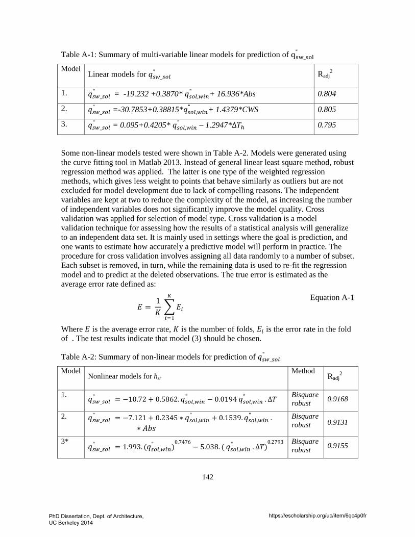
142

Table A-1: Summary of multi-variable linear models for prediction of qsw_sol"

Model Linear models for 𝑞𝑞𝑠𝑤_𝑠𝑜𝑙

" Radj2

1. 𝑞𝑞𝑠𝑤_𝑠𝑜𝑙" = -19.232 +0.3870* 𝑞𝑞𝑠𝑜𝑙,𝑤𝑖𝑛" + 16.936*Abs 0.804

2. 𝑞𝑞𝑠𝑤_𝑠𝑜𝑙" =-30.7853+0.38815*𝑞𝑞𝑠𝑜𝑙,𝑤𝑖𝑛" + 1.4379*CWS 0.805

3. 𝑞𝑞𝑠𝑤_𝑠𝑜𝑙" = 0.095+0.4205* 𝑞𝑞𝑠𝑜𝑙,𝑤𝑖𝑛" – 1.2947*∆𝑇ℎ 0.795

Some non-linear models tested were shown in Table A-2. Models were generated using the curve fitting tool in Matlab 2013. Instead of general linear least square method, robust regression method was applied. The latter is one type of the weighted regression methods, which gives less weight to points that behave similarly as outliers but are not excluded for model development due to lack of compelling reasons. The independent variables are kept at two to reduce the complexity of the model, as increasing the number of independent variables does not significantly improve the model quality. Cross validation was applied for selection of model type. Cross validation is a model validation technique for assessing how the results of a statistical analysis will generalize to an independent data set. It is mainly used in settings where the goal is prediction, and one wants to estimate how accurately a predictive model will perform in practice. The procedure for cross validation involves assigning all data randomly to a number of subset. Each subset is removed, in turn, while the remaining data is used to re-fit the regression model and to predict at the deleted observations. The true error is estimated as the average error rate defined as:

𝐸 =

1𝐾

�𝐸𝑖

𝐾

𝑖=1

Equation A-1

Where 𝐸 is the average error rate, 𝐾 is the number of folds, 𝐸𝑖 is the error rate in the fold of . The test results indicate that model (3) should be chosen.

Table A-2: Summary of non-linear models for prediction of 𝑞𝑞𝑠𝑤_𝑠𝑜𝑙"

Model Nonlinear models for hsr

Method Radj

2

1. 𝑞𝑞𝑠𝑤_𝑠𝑜𝑙" = −10.72 + 0.5862.𝑞𝑞𝑠𝑜𝑙,𝑤𝑖𝑛" − 0.0194 𝑞𝑞𝑠𝑜𝑙,𝑤𝑖𝑛" .∆𝑇 Bisquare

robust 0.9168

2. 𝑞𝑞𝑠𝑤_𝑠𝑜𝑙" = −7.121 + 0.2345 ∗ 𝑞𝑞𝑠𝑜𝑙,𝑤𝑖𝑛" + 0.1539.𝑞𝑞𝑠𝑜𝑙,𝑤𝑖𝑛" .

∗ 𝐴𝑏𝑠𝑠 Bisquare robust 0.9131

3* 𝑞𝑞𝑠𝑤_𝑠𝑜𝑙

" = 1.993. (𝑞𝑞𝑠𝑜𝑙,𝑤𝑖𝑛" )0.7476

− 5.038. ( 𝑞𝑞𝑠𝑜𝑙,𝑤𝑖𝑛" . ∆𝑇)0.2793

Bisquare robust 0.9155



http://en.wikipedia.org/wiki/Model_validation

http://en.wikipedia.org/wiki/Model_validation

http://en.wikipedia.org/wiki/Statistics

http://en.wikipedia.org/wiki/Accuracy

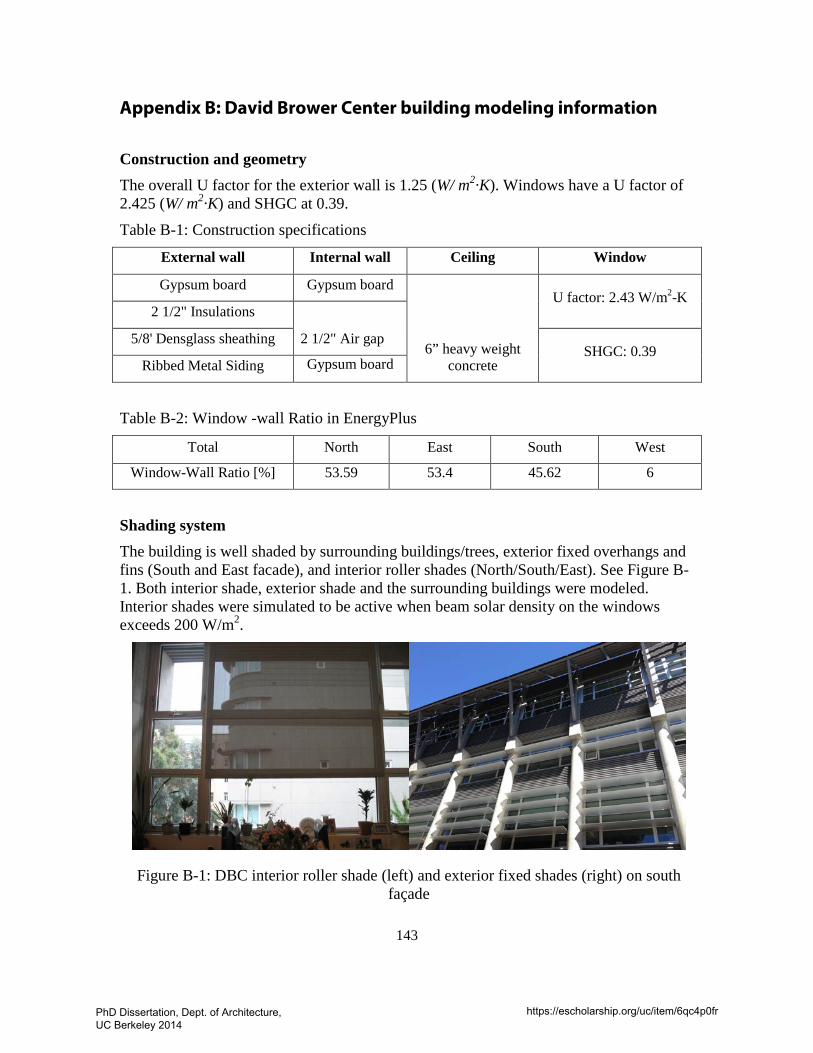
143

Appendix B: David Brower Center building modeling information

Construction and geometry The overall U factor for the exterior wall is 1.25 (W/ m2·K). Windows have a U factor of 2.425 (W/ m2·K) and SHGC at 0.39.

Table B-1: Construction specifications

External wall Internal wall Ceiling Window

Gypsum board Gypsum board

6” heavy weight concrete

U factor: 2.43 W/m2-K 2 1/2" Insulations

2 1/2" Air gap 5/8' Densglass sheathing SHGC: 0.39

Ribbed Metal Siding Gypsum board

Table B-2: Window -wall Ratio in EnergyPlus

Total North East South West

Window-Wall Ratio [%] 53.59 53.4 45.62 6

Shading system The building is well shaded by surrounding buildings/trees, exterior fixed overhangs and fins (South and East facade), and interior roller shades (North/South/East). See Figure B-1. Both interior shade, exterior shade and the surrounding buildings were modeled. Interior shades were simulated to be active when beam solar density on the windows exceeds 200 W/m2.

Figure B-1: DBC interior roller shade (left) and exterior fixed shades (right) on south façade



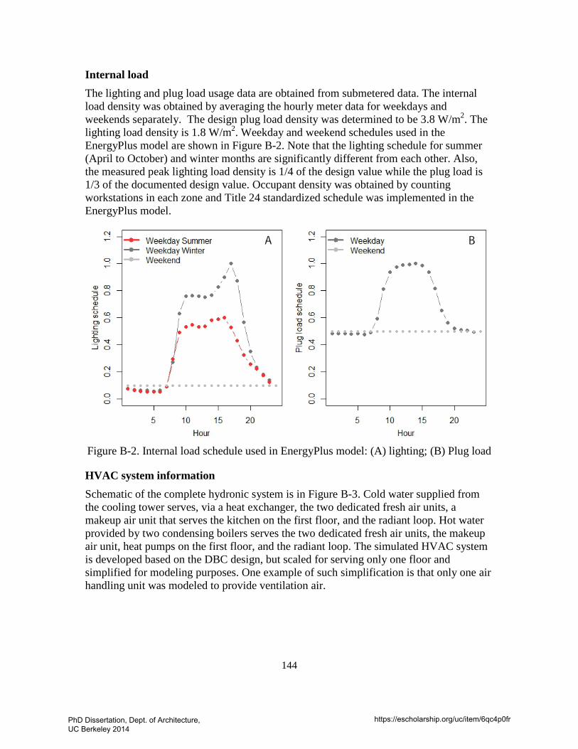
144

Internal load The lighting and plug load usage data are obtained from submetered data. The internal load density was obtained by averaging the hourly meter data for weekdays and weekends separately. The design plug load density was determined to be 3.8 W/m2. The lighting load density is 1.8 W/m2. Weekday and weekend schedules used in the EnergyPlus model are shown in Figure B-2. Note that the lighting schedule for summer (April to October) and winter months are significantly different from each other. Also, the measured peak lighting load density is 1/4 of the design value while the plug load is 1/3 of the documented design value. Occupant density was obtained by counting workstations in each zone and Title 24 standardized schedule was implemented in the EnergyPlus model.

Figure B-2. Internal load schedule used in EnergyPlus model: (A) lighting; (B) Plug load

HVAC system information Schematic of the complete hydronic system is in Figure B-3. Cold water supplied from the cooling tower serves, via a heat exchanger, the two dedicated fresh air units, a makeup air unit that serves the kitchen on the first floor, and the radiant loop. Hot water provided by two condensing boilers serves the two dedicated fresh air units, the makeup air unit, heat pumps on the first floor, and the radiant loop. The simulated HVAC system is developed based on the DBC design, but scaled for serving only one floor and simplified for modeling purposes. One example of such simplification is that only one air handling unit was modeled to provide ventilation air.



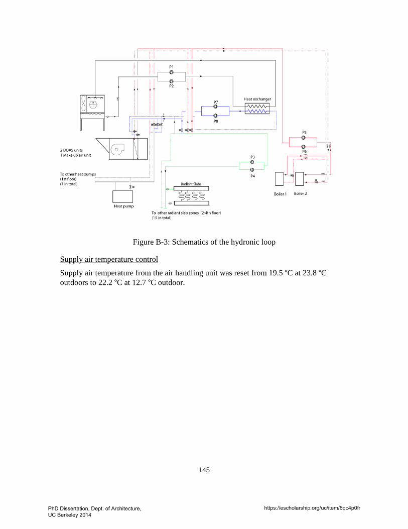
145

Figure B-3: Schematics of the hydronic loop

Supply air temperature control

Supply air temperature from the air handling unit was reset from 19.5 °C at 23.8 °C outdoors to 22.2 °C at 12.7 °C outdoor.



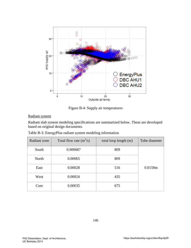
146

Figure B-4: Supply air temperatures

Radiant system

Radiant slab system modeling specifications are summarized below. These are developed based on original design documents.

Table B-3: EnergyPlus radiant system modeling information

Radiant zone Total flow rate (m3/s) total loop length (m) Tube diameter

South 0.000687 809

0.0159m

North 0.00065 809

East 0.00028 516

West 0.00024 435

Core 0.00035 675



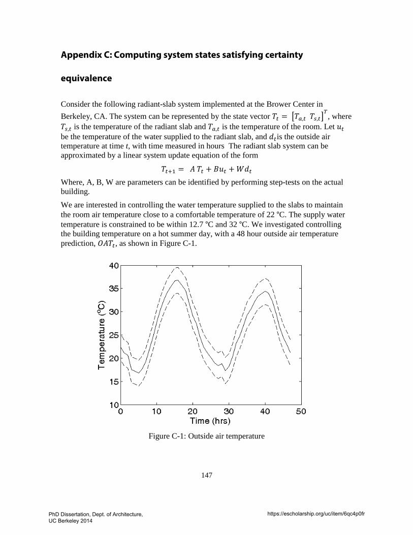
147

Appendix C: Computing system states satisfying certainty

equivalence

Consider the following radiant-slab system implemented at the Brower Center in Berkeley, CA. The system can be represented by the state vector 𝑇𝑡 = �𝑇𝑎,𝑡 𝑇𝑠,𝑡�

𝑇, where

𝑇𝑠,𝑡 is the temperature of the radiant slab and 𝑇𝑎,𝑡 is the temperature of the room. Let 𝑠𝑠𝑡 be the temperature of the water supplied to the radiant slab, and 𝑑𝑡is the outside air temperature at time t, with time measured in hours The radiant slab system can be approximated by a linear system update equation of the form

𝑇𝑡+1 = 𝐴 𝑇𝑡 + 𝐵𝑠𝑠𝑡 + 𝑊𝑑𝑡 Where, A, B, W are parameters can be identified by performing step-tests on the actual building.

We are interested in controlling the water temperature supplied to the slabs to maintain the room air temperature close to a comfortable temperature of 22 °C. The supply water temperature is constrained to be within 12.7 °C and 32 °C. We investigated controlling the building temperature on a hot summer day, with a 48 hour outside air temperature prediction, 𝑂𝐴𝑇𝑡, as shown in Figure C-1.

Figure C-1: Outside air temperature



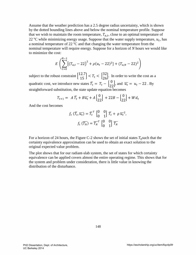
148

Assume that the weather prediction has a 2.5 degree radius uncertainty, which is shown by the dotted bounding lines above and below the nominal temperature profile. Suppose that we wish to maintain the room temperature, 𝑇𝑎,𝑡, close to an optimal temperature of 22 °C while minimizing energy usage. Suppose that the water supply temperature, 𝑠𝑠𝑡, has a nominal temperature of 22 °C and that changing the water temperature from the nominal temperature will require energy. Suppose for a horizon of N hours we would like to minimize the cost:

𝐸 ��(𝑇𝑎,𝑡 − 22�2

+ 𝜌(𝑠𝑠𝑡 − 22)2]𝑁−1

𝑡=0

+ (𝑇𝑎,𝑁 − 22)2�

subject to the robust constraint �12.715 � < 𝑇𝑡 < �32

26�. In order to write the cost as a

quadratic cost, we introduce new states 𝑇𝑡� = 𝑇𝑡 − � 022�, and 𝑠𝑠𝑡�� = 𝑠𝑠𝑡 − 22 . By

straightforward substitution, the state update equation becomes

𝑇𝑡+1 = 𝐴 𝑇𝑡� + 𝐵𝑠𝑠𝑡�� + 𝐴 � 022� + 22𝐵 − � 0

22� + 𝑊𝑑𝑡

And the cost becomes

𝑠𝑠𝑡 (𝑇𝑡� ,𝑠𝑠𝑡��) = 𝑇𝑡�𝑇 �0 0

0 1� 𝑇𝑡� + ρ 𝑠𝑠𝑡��2,

𝑠𝑠𝑡 (𝑇𝑁��) = 𝑇𝑁��𝑇 �0 0

0 1� 𝑇𝑁��

For a horizon of 24 hours, the Figure C-2 shows the set of initial states 𝑇0such that the certainty equivalence approximation can be used to obtain an exact solution to the original expected value problem.

The plot shows that for our radiant-slab system, the set of states for which certainty equivalence can be applied covers almost the entire operating regime. This shows that for the system and problem under consideration, there is little value in knowing the distribution of the disturbance.



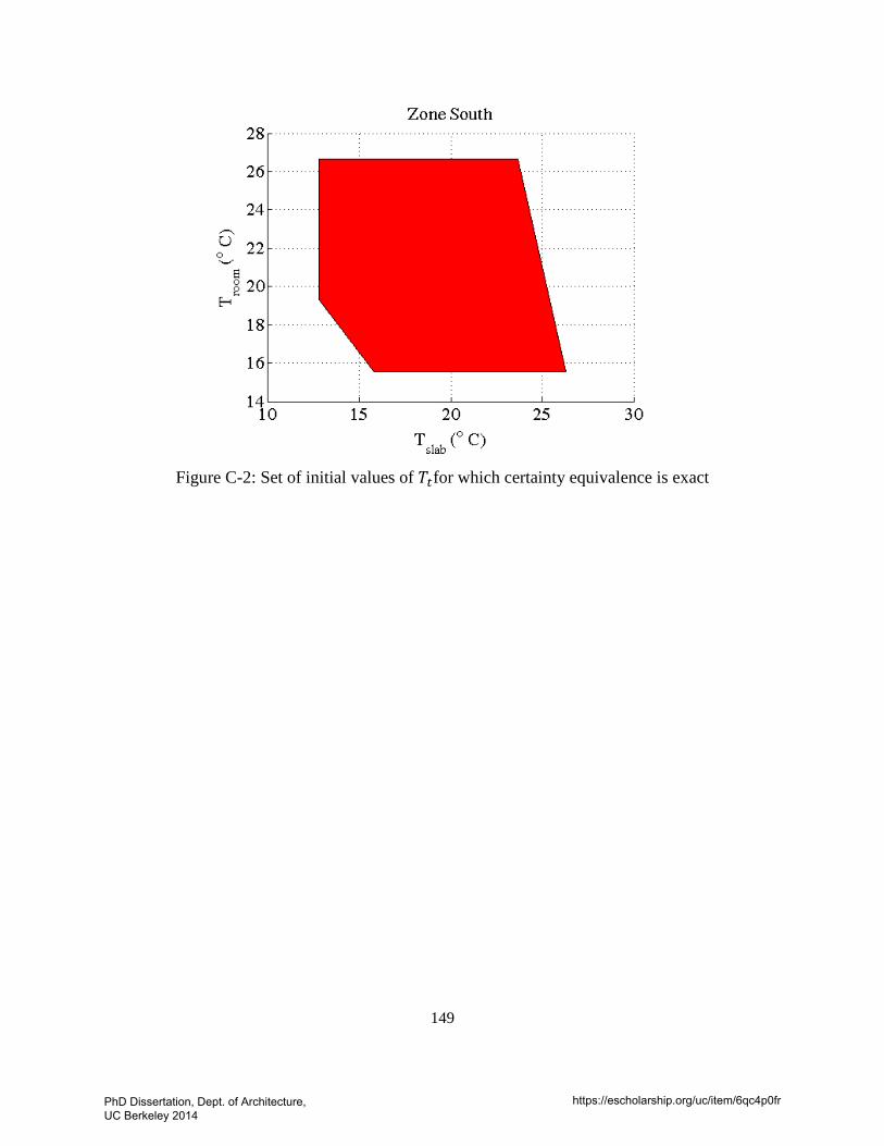
149

Figure C-2: Set of initial values of 𝑇𝑡for which certainty equivalence is exact



design and control of hydronic radiant cooling systemsescholarship.org/uc/item/6qc4p0fr.pdf ·...

Documents