design and development of a by - doras - dcudoras.dcu.ie/576/1/dob_52152677_meng_thesis.pdf ·...
TRANSCRIPT

Design and Development of a Radial Vortex Flow Control Device
By
Dermot O’Brien (B.Eng M.I.E.I.)
Thesis presented at Dublin City University for the Degree of Master of Engineering
Under the Supervision of Dr. Brian Corcoran
School of Mechanical
and Manufacturing Engineering
June 2008

Preface
Declaration…………………………………………………………………………………(i)
Acknowledgements……………………………………………………………………….(i)
Table of Contents………………………………………………………………………… (ii – iv)
List of Figures……………………………………………………………………………. (v - vii)
List of Tables …………………………………………………………………………….. (viii)
Abstract……………………………………………………………………………………. (ix)

i
Declaration / Acknowledgements
Declaration I hereby certify that this material, which I now submit for assessment on the program of
study leading to the award of Master of Engineering is entirely my own work, except where
otherwise stated, and has not been submitted in whole or part to any other university.
Date: 20 / 06 / 2008
Signed …………………………………………
Dermot O’Brien
Student Number: 52152677
Acknowledgements The author would like to thank the following people for the work, time, support and advice
they provided during the course of this project.
Dr. Brian Corcoran
Mr. Colm Concannon
Mr. John Concannon
Mr. Derek Sweeney

ii
Table of Contents
Chapter 1 Introduction & Literature Survey
1.1 Introduction………………………………………………………….………….... 1
1.2 Flooding……………..……………………………………………………………. 2
1.3 Sustainable Urban Drainage Systems………………………………………… 3
1.4 Infiltration / Soak-away………………………………………………………... 4
1.5 Storage and Attenuation………………………………………………………... 4
1.6 Stormwater Flow Control Devices…………………………………………….. 5
1.6.1 Orifice Plate………………………………………………………………5
1.6.2 Flow Valve..………………………………………………………………6
1.6.3 Steinscruv Flow Regulator……………………………..……………….7
1.6.4 HydroSlide………………………………………………………………..8
1.6.5 Vortex Flow Control Devices………………………………………….. 9
1.7 Commercial Flow Control Devices……………………...…………….. ……… 11
1.7.1 Hydro-brake (Hydro International)………..………………….. ……… 11
1.7.2 Hydro-Vex……………………………………………………………….. 12
1.7.3 Mosbaek Flow Control……………………………..………………….. 13
1.7.4 Hydro-brake (Vortechnics)…………………………………………….. 13
1.8 The Vortex……………………………………………………………………….. 14
1.8.1 Vortex Motion……………………………………………………………. 15
1.9 Computational Fluid Dynamics ……………………………………………….. 16
1.10 Aims and Objectives…………...……………………………………………….. 17
1.10.1 Aims……………………………………………………………………… 17
1.10.2 Objectives……………………………………………………………….. 17
Chapter 2 Conceptual and Detailed Design
2.0 Introduction……………………………………………………………………………….. 18
2.1 Industry Standard………………………………………………………………………… 18
2.2 Product Design Specification…………………………………………………………… 19
2.2.1 Performance………………………………………………………………………19
2.2.2 Manufacturability………………………………………………………………… 19
2.2.3 Assembly…………………………………………………………………………. 19
2.3 Mounting Concept 1……………………………………………………………………… 20
2.3.1 Installation………………………………………………………………………... 20
2.4 Mounting Concept 2……………………………………………………………………… 22
2.4.1 Installation………………………………………………………………………... 22
iii
Table of Contents
2.5 Mounting Concept 3……………………………………………………………………… 24
2.5.1 Installation………………………………………………………………………... 25
2.6 Mounting Concept Selection.…………………………………………………………… 26
2.7 Vortex Chamber Design.………………………………………………………………… 27
2.7.1 Manufacturing Process and Material Selection………………………………. 28
2.7.2 Fabrication of the Vortex Chamber……………………………………………. 29
2.8 Mounting Coupler Detailed Design…………………………………………………….. 30
2.8.1 Features………………………………………………………………………….. 30
2.9 Vortex Valve Assembly………………………………………………………………….. 31
2.10 Vortex Valve Installation………………………………………………………………… 32
Chapter 3 Test Rig Design, Development and Initial Testing
3.0 Introduction……………………………………………………………………………….. 33
3.1 Objectives…………………………………………………………………………………. 33
3.2 Test Rig Manhole………………………………………………………………………… 33
3.2.1 Manhole Specification…………………………………………………………... 34
3.3 Flow Measurement Device and Water Holding Tank...……………………………… 35
3.3.1 Weighing Scales and Holding Tank Specification…………………………… 35
3.4 Water Supply to Manhole……………………………………………………………….. 36
3.4.1 Header Tank Specification……………………………………………………... 37
3.5 Test Rig Assembly……………………………………………………………………….. 38
3.6 Test Procedure………………………………………………………...………………….39
3.7 Test Rig Performance Test……………………………………………………………… 41
3.8 Initial Vortex Valve Prototype Geometry………………………………………………. 41
3.9 Initial Vortex Valve Prototype Performance...…………………………………………. 42
Chapter 4 Detailed Testing, Modeling and CFD 4.0 Introduction…………………………………………………………………….................43
4.1 Varying the Vortex Valve Outlet Diameter…………………………………………….. 44
4.1.1 Satisfying Design Objectives…………………………………………………… 45
4.1.2 Relationship Analysis…………………………………………………………… 46
4.1.3 Summary…………….…………………………………………………………… 47
4.2 Varying the Vortex Valve Width…………..…………………………………………….. 48
4.2.1 Satisfying Design Objectives…………………………………………………… 49
4.2.2 Relationship Analysis…………………………………………………………… 50
4.2.3 Summary…………….…………………………………………………………… 51

iv
Table of Contents
4.3 Varying the Vortex Valve Inlet Height.…..…………………………………………….. 52
4.3.1 Satisfying Design Objectives…………………………………………………… 53
4.3.2 Relationship Analysis…………………………………………………………… 54
4.3.3 Summary…………….…………………………………………………………… 55
4.4 Establishing the Relationship Between Geometric Variables……………………….. 56
4.4.1 Outlet Opening Diameter……………………………………………………….. 56
4.4.2 Width of the Vortex Valve………………………………………………………. 56
4.4.3 Inlet Height of the Vortex Valve………………………………………………... 56
4.5 Varying the Swirl Diameter…………………………………………………...…………. 57
4.5.1 Relationship Analysis…………………………………………………………… 58
4.5.2 Summary of Increasing the Swirl Diameter of the Vortex Valve…………… 60
4.6 Vortex Valve Geometry Modeling………………………………………………………. 61
4.6.1 Example………………………………………………………………………….. 62
4.7 Vortex Valve Performance Curve Modeling…………………………………………… 63
4.7.1 Unique Swirl Diameter Vortex Valves…………………………………………. 63
4.7.2 Standard Swirl Diameter Vortex Valves………………………………………. 66
4.8 Limitations Experienced During Testing………………………………………………. 67
4.9 Computational Fluid Dynamics…………………………………………………………. 69
4.9.1 Model Setup................................................................................................. 69
4.9.2 CFD Verification…………………………………………………………………. 75
Chapter 5 Conclusions and Recommendations 5.0 Conclusions………………………………….…………………………………………… 77
5.1 Recommendations………………………...…………………………………………… 79
Chapter 6 References………………………………………………………………..……. 80

v
List of Figures
Chapter 1 Introduction and Literature Survey Figure 1.1 Flooding in Enniscorthy, Co. Wexford
Figure 1.2 Orifice Plate
Figure 1.3 Flow Valve
Figure 1.4 Steinscruv Flow Regulator
Figure 1.5 Hydro-Slide
Figure 1.6 Performance Curve
Figure 1.7 Radial Vortex Valve
Figure 1.8 Conical Vortex Valve
Figure 1.9 Typical Performance Curve
Figure 1.10 Hydro-brake by Hydro International
Figure 1.11 Hydro-Vex
Figure 1.12 Water Brake
Figure 1.13 hydro-brake by Vortechnics
Figure 1.14 Concentric, Asymmetric and Spatial Vortex Motion
Figure 1.15 (a) forced vortex and (b) free vortex
Figure 1.16 CFD Analysis Example
Chapter 2 Conceptual and Detailed Design
Figure 2.1 Standard Radial Vortex Valve Mounting
Figure 2.2 Mounting Concept 1
Figure 2.3 Mounting Concept 1 Installation
Figure 2.4 Mounting Concept 2
Figure 2.5 Mounting Concept 2 Installation
Figure 2.6 Mounting Concept 3
Figure 2.7 Mounting Concept 3 Installation
Figure 2.8 Current Vortex Chamber Geometry
Figure 2.9 New Vortex Chamber Geometry
Figure 2.10 Manufacturing Process Selection Graph
Figure 2.11 Exploded Vortex Chamber View
Figure 2.12 Assembled Vortex Chamber
Figure 2.13 Vortex Valve
Figure 2.14 Vortex Valve Exploded
Figure 2.15 Photo of Actual Vortex Valve
Figure 2.16 Vortex Valve Installed in Ø1.2m manhole

vi
List of Figures
Chapter 3 Test Rig Development and Initial Testing
Figure 3.1 Test Rig Manhole
Figure 3.2 Test Rig Holding Tank and Weighing Scales
Figure 3.3 Raised Header Tank
Figure 3.4 Test Rig Assembly
Figure 3.5 Photograph of Test Rig
Figure 3.6 Initial Prototype
Figure 3.7 Initial Prototype Performance Curve
Figure 3.8 Air Pocket in Vortex Chamber
Chapter 4 Detailed Testing, Modelling and CFD
Figure 4.1 Area A on Typical Performance Curve
Figure 4.2 Varying the Outlet Diameter
Figure 4.3 Outlet Diameter and Orifice Plate Relationship
Figure 4.4 Outlet Diameter and Flow Relationship
Figure 4.5 Outlet Opening Diameter and Head Relationship
Figure 4.6 Varying the Width of the Vortex Valve
Figure 4.7 Vortex Valve Width and Orifice Plate Relationship
Figure 4.8 Outlet Diameter and Flow Relationship
Figure 4.9 Width and Orifice Plate Relationship
Figure 4.10 Variable Inlet Height Analysis
Figure 4.11 Vortex Valve Inlet Height and Orifice Plate Relationship
Figure 4.12 Inlet Height and Flow Relationship
Figure 4.13 Inlet Height and Head Height Relationship
Figure 4.14 Prototype Geometry
Figure 4.15 Varying the Swirl Diameter
Figure 4.16 Swirl Diameter and Orifice Plate Relationship
Figure 4.17 Swirl Diameter and Flush Flow / Kickback Flow Relationship
Figure 4.18 Swirl Diameter and Flush Flow / Kickback Flow Head
Figure 4.19 Linear Equation Swirl Diameter and Orifice Plate Relationship
Figure 4.20 Vortex Valve Calculator
Figure 4.21 Linear relationship example at 1000mm
Figure 4.22 Vortex Valve Calculator Generated Performance Curve
Figure 4.23 CFD Mesh
Figure 4.24 Solver Output Window

vii
List of Figurers
Figure 4.25 CFD Streamlines and Vectors
Figure 4.26 CFD Pressure Plot
Figure 4.27 Initial CFD Correlation
Figure 4.28 Final CFD Correlation

viii
List of Tables
Chapter 2 Conceptual and Detailed Design
Table 2.1 Concept Selection
Chapter 3 Test Rig Development and Initial Testing
Table 3.1 Cost Comparison on Water Supply
Chapter 4 Detailed Testing, Modelling and CFD
Table 4.1 Cross Sectional Area Analysis
Table 4.2 Width Analysis
Table 4.3 Inlet Height Analysis
Table 4.4 Results from Section 4.5
Table 4.5 Mesh Settings
Table 4.6 Advanced Mesh Settings
Table 4.7 Boundary Conditions on Walls
Table 4.8 Boundary Conditions on Openings
Table 4.9 Modified Mesh Settings
ix
Abstract
There has been a noticeable increase in flooding throughout Ireland in recent years, this is
due to global climate change and increased urban development not allowing rainwater
soak into the ground as it once did. This rainwater is then piped to the nearest
watercourse or storm drain contributing to flooding during periods of heavy rainfall.
This project looks at the design, development and testing of a radial vortex flow control
device which is use to limit the rate the rainwater leaves a particular site or development
so as to help minimize downstream flooding.
A number of design concepts were developed along with a test rig to test the performance
of the final design and investigate the influence of changing geometric variables had on
the performance characteristics of the device. Two models were built to predict the
geometric size of the unit under a given specification. An investigation was carried out to
determine if computational fluid dynamics could be used to simulate the flow the vortex
valve.
1
Chapter 1 Introduction & Literature Survey
1.1 Introduction
Over the past ten to fifteen years the Irish landscape has changed radically with the Celtic
Tiger transforming thousands of acres of green fields into developed sites for either
residential, industrial or commercial use. A large percentage of these developments are
adjacent to many of our villages, towns and cities changing their landscape dramatically.
Once a site is developed a huge amount of ground becomes impermeable preventing the
rainwater soaking into the soil as would have happened pre development. Historically this
water is collected in gullies and piped to the nearest water course or storm drain. The
building boom coupled with global climate change has seen a huge amount of storm water
runoff piped directly to the watercourse or storm drain which has caused conventional
systems to become overloaded contributing to large scale flooding in many regional
villages, towns and cities [1].
Local authorities now require a storm water management system be installed on each
new development to limit the amount of storm water runoff, to that of a pre development
rate as outlined in the greater Dublin strategic drainage survey [2]. This is achieved by
slowing down or attenuating the water as it leaves the site and enters the storm drain or
water course. A large tank (usually underground) stores the excess water during a rain
storm while a flow control device limits the discharge to a pre development level.
The most effective and widely used flow control device is a vortex flow control device [3]
which limits the discharge rate as a function of head i.e. height of water in the tank. One of
the main reasons this type of flow control device is so popular is that the orifice opening is
3-6 times the cross sectional area of a conventional orifice plate. The unit has no moving
parts and controls the flow through its geometrical relationships so therefore each unit is
customized to site specific conditions based on flow rate and head height [3].
This project looks at the design and development of a radial vortex flow control device and
aims to 1) Improve the method of installation 2) Investigate the geometrical relationships
3) Build a model that predicts the performance curve and geometric size for a given
specification and 4) Investigate if Computational Fluid Dynamics (CFD) can be used to
simulate flow through the vortex valve based on experimental results.

2
Introduction & Literature Survey
1.2 Flooding
Flooding has become a major problem in Ireland over the last number of years [1] with
many towns and villages being flooded during periods of heavy rainfall. This flooding can
be mainly attributed to two things;
• Increased urban development
• Global climate change
Irelands Celtic tiger economy has seen a considerable increase in the building industry
and in particular urban development. This urban development has transformed green field
sites into large residential, industrial and commercial facilities.
In the past, heavy rainstorms on these green field sites infiltrated into the ground as
nature intended. But with increased urban development this process was interrupted,
heavy rainstorms could no longer infiltrate into the ground because of impermeable
materials such as concrete, tarmac, asphalt, roofs, etc.
Instead all the stormwater generated from these surfaces was piped to the nearest water
course (river) or storm drain. This increased runoff coupled with global climate change has
led to increased flooding due to conventional storm water drainage systems being
overloaded. An example of such flooding can be seen below when the river Slaney in
Enniscorthy burst it’s banks in 2003 after extremely heavy rainfall.
Figure 1.1 - Flooding in Enniscorthy, Co. Wexford (Courtesy of the OPW)

3
Introduction & Literature Survey
1.3 Sustainable Urban Drainage System (SuDS)
Sustainable Urban Drainage Systems (SuDS) is a direct response to the problem of flash
flooding and is defined by the Construction Industry Research and Information Association
(CIRIA) as “a sequence of management practices and control structures designed to drain
surface water in a more sustainable fashion than some conventional techniques”. These
techniques are as applicable to rural settings as they are to urban areas. [4]
Using SuDS techniques, water is either infiltrated or conveyed more slowly to water
courses via ponds, swales, infiltration systems, attenuation tanks or other installations to
try and closely mimic natural catchment drainage behaviour. Run off is frequently delayed
in natural ponds or hollows. In addition to delaying the rate of runoff, there is more
likelihood in the natural situation that pollutants will be filtered through soils or broken
down by bacteria. By mimicking this, SuDS attenuates stormwater runoff and improves
environmental performance [4].
There are eight main methods by which a Sustainable Urban Drainage System may be
implemented [4].
• Permeable Pavements - Use of porous asphalt, porous paving or similar concepts
to reduce imperviousness thus minimising runoff. Runoff infiltrates to a stone
reservoir where some breakdown of pollutants occurs before controlled discharge
to a drain or watercourse or direct infiltration.
• Filter Drains - A gravel filled trench, generally with a perforated pipe at the base
which conveys runoff to a drain or watercourse. These provide attenuation and
trap sediments.
• Infiltration Trenches/ Soak-away - Gravel or specially engineered trenches
designed to store runoff while letting it infiltrate slowly to the ground. These provide
treatment of runoff through filtration, absorption and microbial decomposition.
• Bio-Retention - These devices are depressions back filled with sand and soil and
planted with native vegetation. They provide filtration, settlement and some
infiltration. Typically under drained with remaining runoff piped back to the
drainage system or watercourse.
• Swales - Grass lined channels designed to convey water to infiltration or a
watercourse. Delays runoff and traps pollutants via infiltration for filtering effects of
vegetation.

4
Introduction & Literature Survey
• Detention Basins - Dry vegetated depressions which impound stormwater during
an event and gradually release it. Mostly for volume control but some pollutant
removal is achieved via settlement of suspended solids and some infiltration.
• Retention Ponds - Permanent water bodies which store excess water for long
periods allowing particle settlement and biological treatment. Very effective for
pollutant removal but limited to larger developments. Have high habitat and
aesthetic benefits.
• Attenuation Tanks – Underground storage tanks on site, either of concrete or
modular plastic construction. These tanks store the excess runoff during a
rainstorm event and release it into the local storm drain or water course at a
controlled rate through the use of a flow control device.
A lot of the above methods are designed for above ground use, because of this a large
area of land is required for their operation. Unfortunately urban development does not
allow for such structures to be put in place in many situations and developers will not use
such land hungry methods of SuDS. Because of this the most common approach is sub
surface (underground) attenuation / infiltration tanks where the ground above the structure
can be used for car parking, amenity area etc.
1.4 Infiltration / Soakaway
Infiltration devices are the first option which should be considered for stormwater disposal.
Only if infiltration is not practical should runoff be disposed of to a watercourse or sewer.
Infiltration allows runoff to be dealt with at source and mimics the natural process of
groundwater recharge. Being buried, the systems often require little or no additional land
take [3].
Infiltration systems are only effective in certain soil types and groundwater levels. They
should only be installed if they will not put groundwater quality and ground stability at risk.
Runoff which is likely to be heavily contaminated should not be disposed of by infiltration.
Land use above and around the devices may need to be restricted to allow maintenance
and prevent structural damage [3].
1.5 Storage and Attenuation
In situations where infiltration is not suitable due to ground conditions, attenuation storage
will still allow the control of peak storm water. Storage allows surface water discharge
from a developed site to mimic run off in its undeveloped state. A range of options are
available and

5
Introduction & Literature Survey
this choice will be influenced by a number of factors including drainage depth, ground
water level, site topography, site usage (car park or building) and space available [3].
All systems require provision of some form of flow control device to mobilize the storage
except where the run off restriction is not onerous or where discharge to natural ground to
replenish the ground water table is feasible. In all cases the site condition and constraints,
as well as discharge licenses stipulated by regulating body, must be properly understood
before the preferred system can be specified [3].
All of the systems are relatively easy to maintain, although certain modular systems and in
situ tanks could allow silt to enter and may be more difficult to clean than conventional
piped systems. Some modular systems recommend putting a large silt collection device
upstream of the storage facility to catch the silt before it reaches the tank.
1.6 Storm Water Flow Control Devices There are a number of flow control devices that will regulate or control stormwater from a
storage or attenuation system. The operation of a number of devices are detailed below
with the advantages and disadvantages of each being outlined.
1.6.1 Orifice Plate An orifice plate is the simplest type of flow control device which controls the rate of fluid
flow. It states that ”there is a relationship between the pressure of the fluid and the velocity
of the fluid - velocity increases, the pressure decreases and vice versa”. This principle is
based on Bernoulli’s equation and is one of the oldest types of flow control devices. An
orifice plate is a thin plate with a hole in the middle. It is usually placed in a pipe in which
fluid flows [5].
Figure 1.2 - Orifice Plate (Courtesy of Efunda)

6
Introduction & Literature Survey
As fluid flows through the pipe it has a certain velocity (which we want to measure) and a
certain pressure (which is quite easily measured). When the fluid reaches the orifice plate,
with the hole in the middle, the fluid is forced to converge and go through the small hole;
the point of maximum convergence is actually just after the physical orifice, at the so-
called "vena contracta" point (see figure 1.2). As it does so, the velocity and the pressure
changes. By measuring the difference in fluid pressure between the normal pipe section
and at the vena contracta, we can find the velocity of the fluid flow by applying Bernoulli's
equation [5].
Advantages
• Inexpensive
• Simple calculation to determine orifice diameter
Disadvantages
• Prone to blockages due to small orifice diameter
• Increases storage requirements when compared with other flow control devices
1.6.2 Flow Valve The flow valve was developed in the late 1970’s in Sweden as a device for holding the
outflow from a detention facility constant. The flow control device is essentially a central
outlet pipe surrounded by a pressure chamber filled with air as shown in figure 1.3. The
top part of the pressure chamber and its connection to the central outlet pipe are made of
flexible rubber fabric; the rubber fabric is braced at the inlet and outlet of the centre pipe
[6].
Figure 1.3 - Flow Valve

7
Introduction & Literature Survey
Water pressure on the upper portion of the rubber fabric is propagated through the
pressure chamber displacing the fabric at the outlet section. Thus, the hydraulic capacity
of the outlet is throttled by the change in cross sectional area. The resultant effect is that
the discharge through the flow valve remains constant and independent of pressure [6].
Advantages
• Discharge independent of pressure
Disadvantages
• Prone to blockages due to small orifice diameter
• Expensive
• Not commonly used
1.6.3 Steinscruv Flow Regulator The Steinscruv flow regulator was developed in Sweden in the mid-1970s for temporarily
impounding flow in pipelines. The flow regulator consists of a stationary, anchored screw
shaped plate that is turned through 270° and installed in a pipe, as shown in figure 1.4
below [6].
In the part of the plate which fits against the bottom of the pipeline, there is an opening to
release a certain specified base flow. The opening is sized so that the flow that passes
through the regulator is sufficient to maintain the self cleansing velocity of the pipeline.
Damming takes place when the inflow to the regulator exceeds the capacity of the base
opening. The extent of this damming and the volume detained are dependent on the slope
of the pipe. When the flow depth reaches the crown of the pipe, the flow capacity
becomes practically equal to the unregulated capacity. It is possible to further regulate the
flow by using several flow regulators in series [6].
Figure 1.4 - Steinscruv Flow Regulator

8
Introduction & Literature Survey Advantages
• At full bore the flow becomes almost equal to the unregulated capacity
Disadvantages
• Complex internal components
• Expensive
• Not commonly used
1.6.4 Hydro-Slide The Hydro-slide regulator was commercially developed in Germany in the 1990’s with a
number of patents attached to its design. The device controls the flow by allowing the
head of water in the detention facility to raise a float as shown in figure 1.5. This in turn
opens an orifice the required amount to control the flow passing through [7].
Figure 1.5 - Hydro-Slide (Courtesy of Copa)
The Hydro-Slide does not affect the flow until it is approaching the set discharge limit, this
allows fluid to be discharged to the watercourse for flows below the set point, hence
slowing the build up of head in the detention tank and therefore maximizing the onsite
detention volume.
The graph below in figure 1.6 shows the performance of the Hydro-slide compared with a
vortex valve and orifice plate. The Hydro-slide operates efficiently but is very prone to
blockage because of the small size of the orifice opening when compared with a vortex
valve. In comparison the Hydro-slide is expensive because of its stainless steel casing
and complex mechanical operation [7].

9
Introduction & Literature Survey
Head
Hei
ght (
m)
Flow (l/s) Figure 1.6 - Performance Curve (Courtesy of Copa)
Advantages
• Design flow rate reached at low head
• Very efficient for large head heights
Disadvantages
• Prone to blockages due to small orifice diameter
• Expensive
• Complex internal components
1.6.5 Vortex Flow Control Devices Vortex Flow Control devices were developed in Denmark in the mid-1960’s [8] to control
outflow from a storage structure. At low flow rates fluid enters through the inlet and passes
straight to the outlet with no restriction. As the inlet flow increases due to upstream
hydraulic head, an air filled vortex is generated in the unit as shown in figure 1.7 below.
This generates high peripheral velocities which restricts flow and creates a back pressure.
The back pressure restricts flow to the desired rate at a given head height.
Figure 1.7 - Radial Vortex Valve
10
Introduction & Literature Survey
The vortex valve is self activating, requires no external power source and it has an orifice
opening much larger than conventional flow control devices. This large opening coupled
with high internal velocities minimise the risk of blockage. The complete absence of
moving parts is also a big advantage with the possibility for mechanical failure minimised.
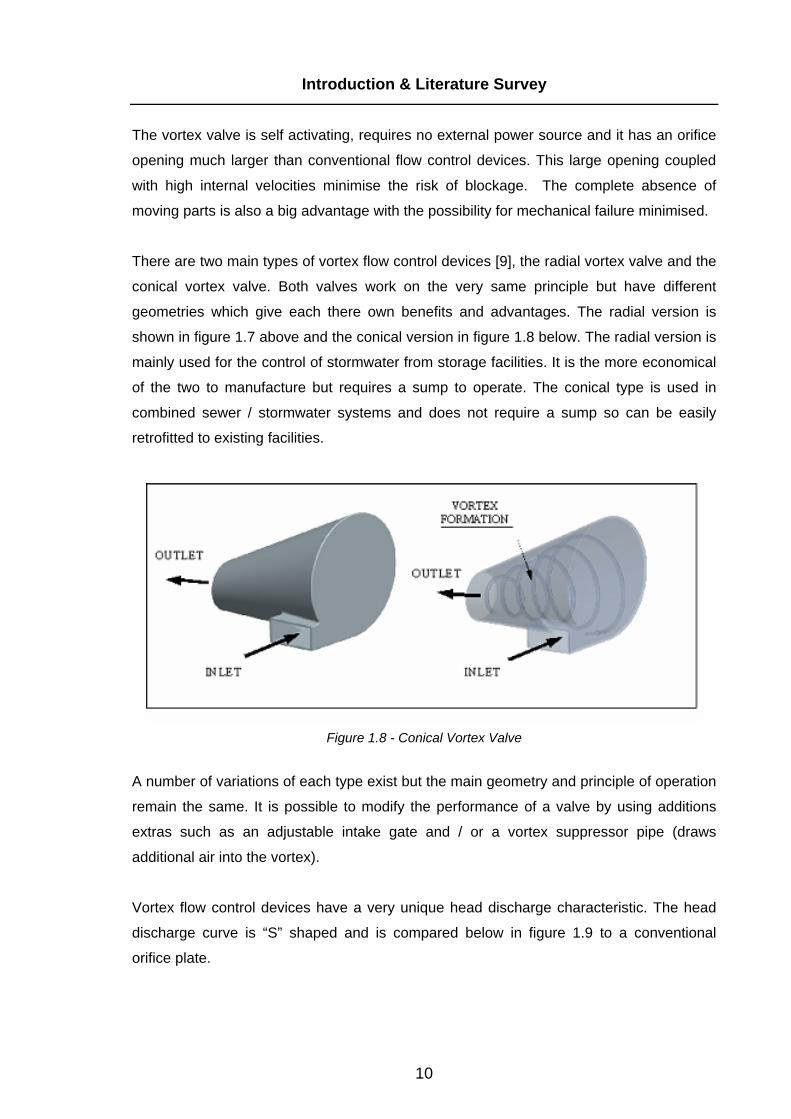
There are two main types of vortex flow control devices [9], the radial vortex valve and the
conical vortex valve. Both valves work on the very same principle but have different
geometries which give each there own benefits and advantages. The radial version is
shown in figure 1.7 above and the conical version in figure 1.8 below. The radial version is
mainly used for the control of stormwater from storage facilities. It is the more economical
of the two to manufacture but requires a sump to operate. The conical type is used in
combined sewer / stormwater systems and does not require a sump so can be easily
retrofitted to existing facilities.
Figure 1.8 - Conical Vortex Valve
A number of variations of each type exist but the main geometry and principle of operation
remain the same. It is possible to modify the performance of a valve by using additions
extras such as an adjustable intake gate and / or a vortex suppressor pipe (draws
additional air into the vortex).
Vortex flow control devices have a very unique head discharge characteristic. The head
discharge curve is “S” shaped and is compared below in figure 1.9 to a conventional
orifice plate.

11
Introduction & Literature Survey
Typical Performance Curves
0
2 0 0
4 0 0
6 0 0
8 0 0
1 0 0 0
1 2 0 0
1 4 0 0
1 6 0 0
1 8 0 0
2 0 0 0
0 1 2 3 4 5 6 7 8
Flow Rate (l/s)
Hea
d (m
m)
Typical Vortex Valve Typical Orifice Plate
Figure 1.9 - Typical Performance Curve
Advantages
• Outlet orifice cross sectional area is 3-6 times that of an orifice plate so therefore
the possibility of a blockage is minimised
• Unique S shaped discharge curve
• Self Activating and self cleansing
• Available in radial and conical geometry
• Reduces storage requirements of attenuation systems
Disadvantages
• Difficult to install in a standard storm water manhole
• Expensive due to their stainless steel construction
• Limited number of suppliers
• Widely used in industry
1.7 Commercial Vortex Flow Control Devices
There are four main manufacturers of vortex flow control devices around the world. One
based in Britain, one in Canada, one in the USA and one in Sweeden
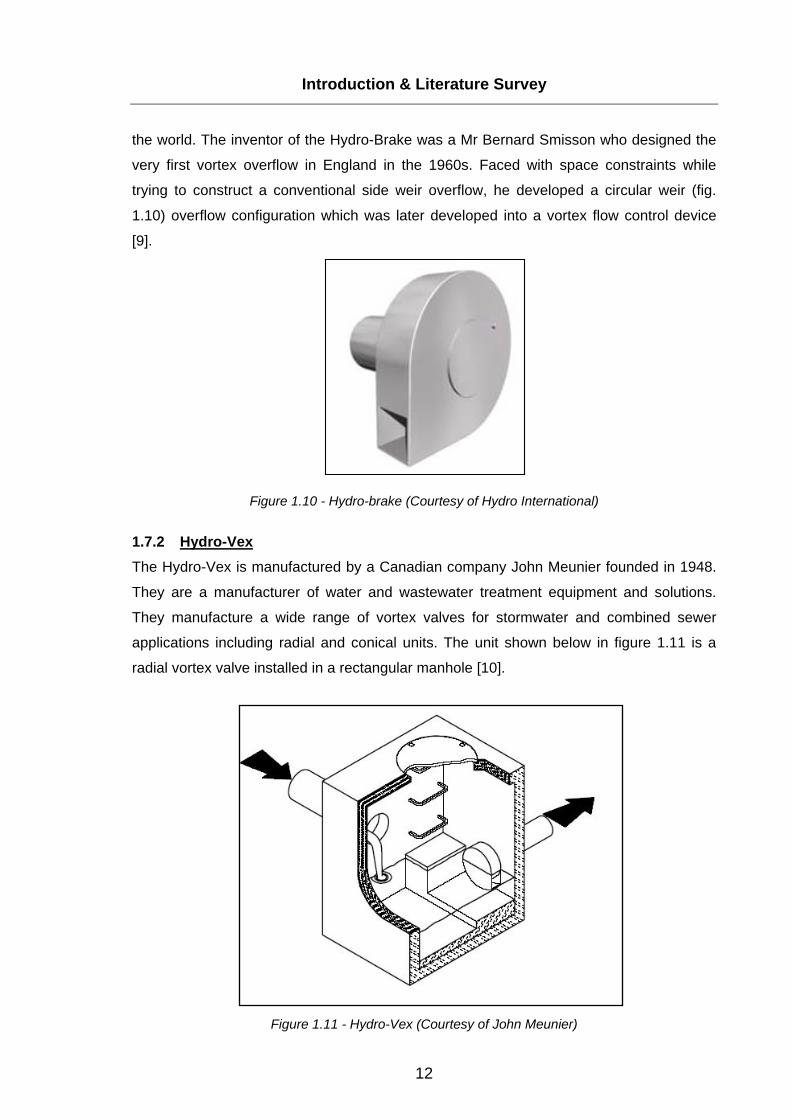
1.7.1 Hydro-Brake (Hydro-International) The Hydro-Brake (fig.1.10) is the most commonly used vortex flow control valve with over
10,000 units installed worldwide. The units are manufactured by Hydro International LTD,
an English company with regional offices in the USA and Ireland. The company was
formed in 1980 to promote hydrodynamic vortex separation and vortex flow control
technology around
12
Introduction & Literature Survey
the world. The inventor of the Hydro-Brake was a Mr Bernard Smisson who designed the
very first vortex overflow in England in the 1960s. Faced with space constraints while
trying to construct a conventional side weir overflow, he developed a circular weir (fig.
1.10) overflow configuration which was later developed into a vortex flow control device
[9].
Figure 1.10 - Hydro-brake (Courtesy of Hydro International)
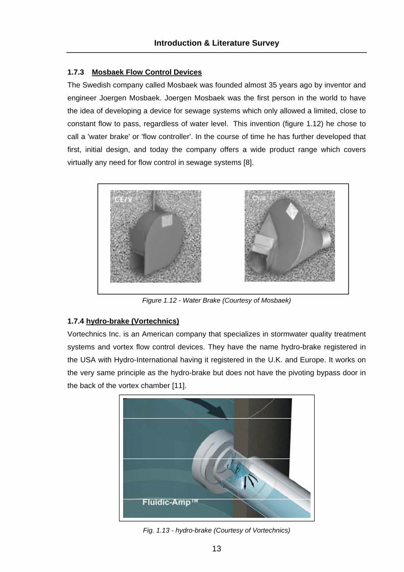
1.7.2 Hydro-Vex The Hydro-Vex is manufactured by a Canadian company John Meunier founded in 1948.
They are a manufacturer of water and wastewater treatment equipment and solutions.
They manufacture a wide range of vortex valves for stormwater and combined sewer
applications including radial and conical units. The unit shown below in figure 1.11 is a
radial vortex valve installed in a rectangular manhole [10].
Figure 1.11 - Hydro-Vex (Courtesy of John Meunier)
13
Introduction & Literature Survey
1.7.3 Mosbaek Flow Control Devices The Swedish company called Mosbaek was founded almost 35 years ago by inventor and
engineer Joergen Mosbaek. Joergen Mosbaek was the first person in the world to have
the idea of developing a device for sewage systems which only allowed a limited, close to
constant flow to pass, regardless of water level. This invention (figure 1.12) he chose to
call a 'water brake' or 'flow controller'. In the course of time he has further developed that
first, initial design, and today the company offers a wide product range which covers
virtually any need for flow control in sewage systems [8].
Figure 1.12 - Water Brake (Courtesy of Mosbaek)
1.7.4 hydro-brake (Vortechnics) Vortechnics Inc. is an American company that specializes in stormwater quality treatment
systems and vortex flow control devices. They have the name hydro-brake registered in
the USA with Hydro-International having it registered in the U.K. and Europe. It works on
the very same principle as the hydro-brake but does not have the pivoting bypass door in
the back of the vortex chamber [11].
Fig. 1.13 - hydro-brake (Courtesy of Vortechnics)

14
Introduction & Literature Survey
1.8 The Vortex
The word vortex comes from the latin word vertex, verticis (m.) meaning "eddy" or "whirlwind". Some of the earliest research on vortex motion was published by Hermann von Helmholtz (1821-1894) in 1858, and by William Thomson, later Lord Kelvin (1824-1907), in 1869. The names of these two giants of classical physics are jointly associated with many of the principal concepts of vortex motion [12]. The exact definition of the word vortex is neither simple nor unique and is dependent upon the distinction being made between a particle rotating about its own axis or one revolving with many other particles around a common axis. For the purpose of this thesis a single particle rotating about its own axis will not be considered and the following definition of a vortex will apply [12].
A vortex is the rotating motion of a multitude of material particles around a common center.
The path of individual particles does not have to be circular, but may also be asymmetrical as shown in figure 1.14. The vortex motions in figure 1.14 (a) and (b) are plane structure’s with their paths the same in every plane normal to the axis of rotation but in nature and technology this is rarely the case and vortex motion is nearly always spatial where the path lines are not perpendicular to the axis of rotation but have a component parallel to it as in figure 1.14 (c). A spatial vortex does not need its path closed as with the concentric and asymmetrical vortex.
(a) (b) (c)
Figure. 1.14 – Concentric, Asymmetric and Spatial Vortex Motion

15
Introduction & Literature Survey
1.8.1 Vortex Motion
There are two main types of plane vortex motion, 1) the potential vortex which is
sometimes called a free vortex and 2) solid body rotation which is often called a forced
vortex. The simplest way to explain the difference between these two vortices is with an
example:
A solid cylindrical rod is rotating at constant velocity in a fluid, after a short period of time
(transient) the fluid velocity is highest and equal to that of the rod at the rods surface since
the fluid adheres to the surface of the rod. With increasing distance from the centre of
rotation the velocity decreases inversely proportional to the distance (see figure 1.15).
Such fluid motion is called a potential vortex. A potential vortex is also irrotational which
means that although the streamlines are circular the individual molecules of the vortex do
not spin as they orbit the axis of the vortex. This can be demonstrated by observing a
cross placed in a potential vortex, the cross rotates about the axis of the vortex but not
around its own axis. Therefore the fluid has no vorticity except at the centre of rotation. A
common everyday example of a potential or free vortex is a bathtub vortex which can be
seen form when a bath of water is emptying [12].
Now consider a hollow tube filled with water rotating a constant velocity about the axis of
the tube, again after a transient period the fluid will rotate like a solid body because of its
adherence to the walls of the tube. The velocity of the fluid increases linearly with distance
from the centre of rotation (see fig.1.15), and the angular velocity is constant everywhere
in the fluid. This type of vortex motion is called solid body rotation or a forced vortex and is
true only when the fluid motion is steady. A common everyday example of a forced vortex
is when a cup of tea is being stirred [12].
Figure 1.15 - (a) forced vortex and (b) free vortex

16
Introduction & Literature Survey
1.9 Computational Fluid Dynamics
Computational Fluid Dynamics (CFD) is a branch of fluid mechanics that uses numerical
methods to solve the governing equations of fluid flow, namely the conservation laws
relating to the transport of mass, momentum and energy. Computers are used to perform
millions of calculations that are required to simulate the interaction of fluids and gases with
surfaces used in engineering. However, even with simplified equations and high-speed
supercomputers, only approximate solutions can be achieved in many cases. Validation of
CFD results is an essential part of CFD for accurate modelling and simulations [13].
CFD has become an essential part of technological advancement in the following areas:
aerospace, automotive, heat transfer, process engineering, hydrodynamics, wind power,
air conditioning and ventilation, hydraulics, sediment transport, biomedical engineering
and electronic cooling. The results of a simple steady state and complex transient analysis
can be seen below.
Figure 1.16 – CFD Analysis Examples
A commercial CFD software package called Ansys CFX was used to perform the
simulations. Ansys CFX is one of the leading CFD software packages available on the
market and simulations are normally performed by experienced engineering analysts
specialising in fluid dynamics. This is due to the complexities involved in model setup and
inaccuracies associated with poor assumptions. For these reasons along with the time
dependent nature of the analysis the author received some guidance from IDAC Ireland in
the setup of the problem using Ansys CFX software [14].
17
Introduction & Literature Survey
1.10 Aim and Objectives The vortex flow control device is the most widely used method for controlling the
discharge rate of storm water. There are only a handful of manufacturers, all of which
keep the design principles closely guarded and are therefore unknown. Currently none of
the designs allow for easy installation in a standard storm water manhole. For these
reasons the following aims and objectives were set out.
1.10.1 Aims
• The main aim of this project is to design and develop a radial vortex flow control
valve for controlling flow from storm water attenuation systems.
1.10.2 Objectives
• To design and develop a number of concepts for the vortex flow control device
along with ways in which they can be easily installed.
• To select a concept and develop a detailed design
• To build working prototypes of the detailed design
• To design and develop a full scale test rig and test a prototype unit.
• To test a number of prototypes and find the influence each of the geometric
variables has on the performance of the device.
• To select a geometric relationship between each of the variables that satisfies the
following:
1. An outlet cross sectional area 3-6 times that of an orifice plate
2. An inlet cross sectional area similar to that of the outlet to minimize
blockage
3. A performance curve that will maximize the flow through the unit
while keeping a large design flow range.
• To build a mathematical model to predict the geometric size of the vortex chamber
and generate a head discharge curve when given a flow rate and head height
specification.
• To investigate if computational fluid dynamics can be used to model the
performance of the radial vortex valve based on experimental results.

18
Chapter 2
Conceptual and Detailed Design
2.0 Introduction Vortex flow control devices by their very nature change in size and geometry depending
upon the required flow rate and specified head height. The design approach was to carry
out the product design specification and base the conceptual design on one particular size
of radial vortex flow control device with the ability to scale up and down the size
depending on the required specification. Three concepts were developed for ways to
mount the vortex valve to the inside of a standard Ø1.2m storm water manhole. Two
concepts were then developed for the shape of the vortex chamber.
2.1 Industry Standard Currently all radial vortex valves in industry are manufactured from stainless steel and
have been for many years [7-11]. All current radial vortex valves on the market also need
to be mounted onto a flat surface so therefore modifications are required to the standard
Ø1.2m storm water manhole found on most construction sites. This means that a custom
rectangular manhole has to be constructed where the vortex valve is to be installed,
alternatively a flat face can be shuttered on a circular manhole as shown blow in figure
2.1. The interface between the vortex valve and the manhole does not have a waterproof
seal which may alter the performance claims of the manufacturer.
Figure 2.1 - Standard Radial Vortex Valve Mounting (Courtesy of Hydro International)

19
Conceptual and Detailed Design
2.2 Product Design Specification
A product design specification was developed to outline all the design and performance
requirements of the vortex valve, this includes identifying the problems associated with
current vortex valves in the market place and setting objectives to alleviate these
problems.
2.2.1 Performance
• The vortex valve must be easily installed into a Ø1.2m manhole ring.
• The vortex valve must be available for installation in a rectangular manhole.
• The vortex valve must provide a watertight seal between the manhole and the
vortex valve.
• The vortex valve must integrate an emergency bypass of the vortex chamber in
the event of a blockage due to some contaminant in the water e.g. large plastic
bag.
• The vortex valve must allow service to the pipe downstream of the manhole.
• The vortex valve must be able to suit an outlet pipe size of up to 300mm.
• The vortex valve must have an expected service life of 50 years in line with the
current specification for storm water pipe.
• The vortex valve must be durable enough the take any general handling and
transportation that may occur on site.
2.2.2 Manufacturability
• The vortex valve is to be fabricated or moulded from a suitable type of plastic, this
makes the unit a lot more economical to manufacture than those available in
stainless steel.
• The plastic vortex valve must provide performance equal to or greater than that of
a stainless steel unit.
2.2.3 Assembly
• The vortex valve is to be assembled using corrosion resistant materials
• The vortex valve will comply with design for assembly guidelines so the product is
easily and economically assembled.

20
Conceptual and Detailed Design
2.3 Mounting - Concept 1
Concept 1 is a vortex valve with a horizontal outlet pipe mounted to a square flange, the
outlet pipe has a vertical tee that acts as an overflow pipe. The overflow pipe must be
equal or greater in length than the head height or top water level. This means that if the
head height ever goes above the design height the unit will automatically by-pass the
valve and flow to the outlet pipe. This feature will never allow the vortex valve to flood up
to ground level unless the overflow pipe also gets blocked.
Outlet Pipe
Vortex Chamber
Overflow Pipe
Flanged Outlet
Figure 2.2 – Mounting Concept 1
2.3.1 Installation Concept 1 may be installed in either a standard Ø1.2m manhole (see figure 2.3) or a
rectangular manhole. For a rectangular manhole a straight outlet flange is required and for
a circular manhole a curved outlet flange is required.
Installation of the unit is as follows:
• Align the flange to the outlet pipe on the inside face of the manhole
• Mark and drill the manhole to take the steel stud anchors
• Fix the flange to the manhole with the steel stud anchors
• Seal around the flange with silicone

21
Conceptual and Detailed Design
Figure 2.3 – Mounting Concept 1 Installation
22
Conceptual and Detailed Design
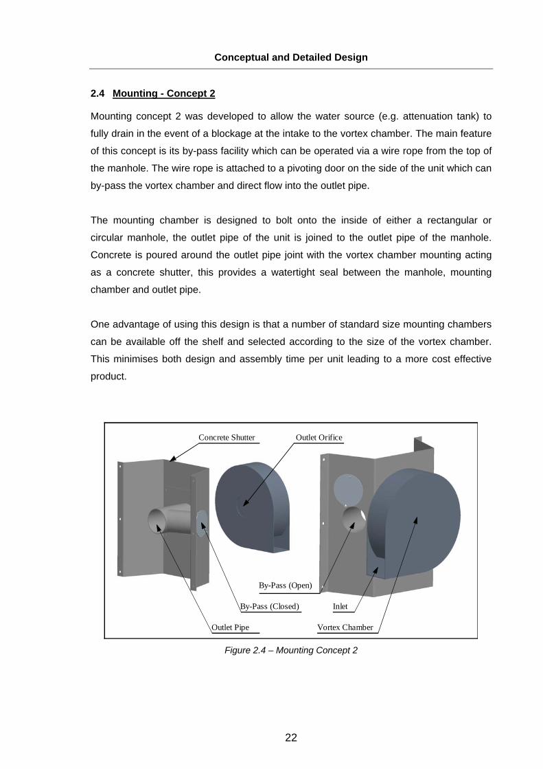
2.4 Mounting - Concept 2
Mounting concept 2 was developed to allow the water source (e.g. attenuation tank) to
fully drain in the event of a blockage at the intake to the vortex chamber. The main feature
of this concept is its by-pass facility which can be operated via a wire rope from the top of
the manhole. The wire rope is attached to a pivoting door on the side of the unit which can
by-pass the vortex chamber and direct flow into the outlet pipe.
The mounting chamber is designed to bolt onto the inside of either a rectangular or
circular manhole, the outlet pipe of the unit is joined to the outlet pipe of the manhole.
Concrete is poured around the outlet pipe joint with the vortex chamber mounting acting
as a concrete shutter, this provides a watertight seal between the manhole, mounting
chamber and outlet pipe.
One advantage of using this design is that a number of standard size mounting chambers
can be available off the shelf and selected according to the size of the vortex chamber.
This minimises both design and assembly time per unit leading to a more cost effective
product.
Vortex Chamber
By-Pass (Closed)
Outlet Pipe
Outlet Orifice Concrete Shutter
By-Pass (Open)
Inlet
Figure 2.4 – Mounting Concept 2

23
Conceptual and Detailed Design
2.4.1 Installation Concept 2 may be installed in either a standard Ø1.2m manhole (see figure 2.5) or a
rectangular manhole.
• Align the concrete shutter to the outlet pipe on the inside face of the manhole.
• Mark and drill the manhole to take the steel stud anchors.
• Fix the concrete shutter to the manhole with the steel stud anchors.
• Connect the manhole outlet pipe to the vortex chamber outlet.
• Fill the shutter with concrete ensuring no seepage into the outlet pipe.
• Mark and drill the underside of the manhole cover.
• Fix the bypass cord bracket the underside of the manhole ensuring the cord
operates freely.
Figure 2.5 – Mounting Concept 2 Installation
The main advantage of the design is the incorporation of a pivoting by-pass door which
allows the vortex chamber to be by-passed in the event of a blockage. The main
disadvantage is the use of concrete to provide a seal between the outlet pipe and the
vortex valve.
24
Conceptual and Detailed Design
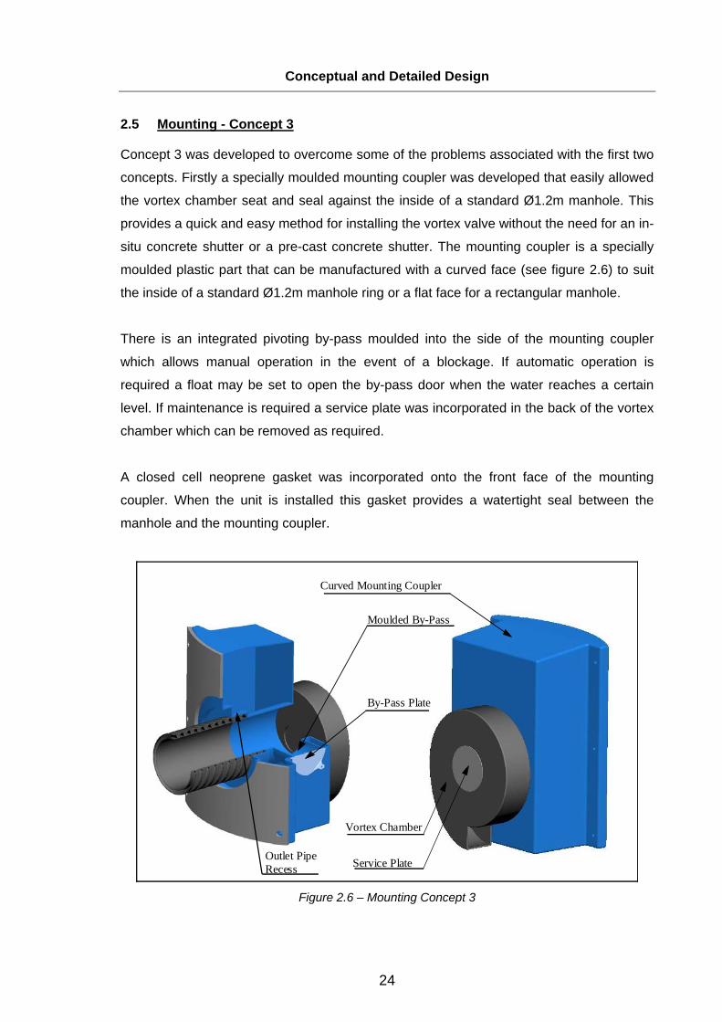
2.5 Mounting - Concept 3
Concept 3 was developed to overcome some of the problems associated with the first two
concepts. Firstly a specially moulded mounting coupler was developed that easily allowed
the vortex chamber seat and seal against the inside of a standard Ø1.2m manhole. This
provides a quick and easy method for installing the vortex valve without the need for an in-
situ concrete shutter or a pre-cast concrete shutter. The mounting coupler is a specially
moulded plastic part that can be manufactured with a curved face (see figure 2.6) to suit
the inside of a standard Ø1.2m manhole ring or a flat face for a rectangular manhole.
There is an integrated pivoting by-pass moulded into the side of the mounting coupler
which allows manual operation in the event of a blockage. If automatic operation is
required a float may be set to open the by-pass door when the water reaches a certain
level. If maintenance is required a service plate was incorporated in the back of the vortex
chamber which can be removed as required.
A closed cell neoprene gasket was incorporated onto the front face of the mounting
coupler. When the unit is installed this gasket provides a watertight seal between the
manhole and the mounting coupler.
By-Pass Plate
Outlet Pipe Recess
Vortex Chamber
Curved Mounting Coupler
Service Plate
Moulded By-Pass
Figure 2.6 – Mounting Concept 3

25
Conceptual and Detailed Design
2.5.1 Installation
Concept 3 can be installed in either a standard Ø1.2m manhole or a rectangular manhole
as required once the correct mounting coupler is selected. The unit is installed as follows:
• Align the mounting coupler with the outlet pipe on the inside face of the manhole.
• Mark and drill the manhole to take the steel stud anchors.
• Fix the mounting coupler to the manhole with the steel stud anchors.
• Mark and drill the underside of the manhole cover.
• Fix the bypass cord bracket to the underside of the manhole ensuring the cord
operates freely.
Figure 2.7 – Mounting Concept 3 Installation
The main advantage of this design is the specially moulded mounting coupler which
ensures quick and easy installation while providing a sealable receiver for the outlet pipe.
It also incorporates a pivoting by-pass door but ensures a watertight connection with the
outlet pipe due to its unique geometry.

26
Conceptual and Detailed Design
2.6 Mounting Concept Selection
Concept selection was not a difficult task as the concepts evolved from one to the next,
possible problems associated with the design were identified and addressed in successive
concepts. Concept three satisfies all the design requirements set out in the product design
specification. A weighted matrix table is shown below to outline the evolution of the design
from concept one to concept three.
Feature Weight (1-5) Concept 1 Concept 2 Concept 3
Installation in a standard Ø1.2m Manhole 5 3 (15) 3 (15) 3 (15)Installation Option in a Rectangular Manhole 3 3 (9) 3 (9) 3 (9)Ease of Installation 4 1 (4) 1 (4) 3 (12)Watertight Seal 2 1 (2) 2 (4) 3 (6)By-pass Facility 4 1 (4) 3 (12) 3 (12)Access for Maintanance 4 1 (4) 1 (4) 3 (12)Service Life & Durability 3 2 (6) 2 (6) 2 (6)Cost 4 3 (12) 2 (8) 1 (4)Total 56 62 76
Table 2.1 (Concept Selection)

27
Conceptual and Detailed Design
2.7 Vortex Chamber Design
The design of the vortex chamber is dependent upon the required flow rate specification.
The principle geometry is the same in all types of radial vortex flow control devices, this
generic shape is a circular chamber with a tangential inlet to initiate a rotational motion
inside the chamber, creating a vortex with a horizontal outlet.
Current geometry as seen on all commercial radial vortex flow control devices is shown in
figure 2.8 below. When analysed part of the design named area ”A” was identified as
having no obvious functional feature. It does not contribute to controlling the flow into the
vortex chamber as this is performed by the inlet height “H”.
Area “A”
H
Internal Component
Figure 2.8 – Current Vortex Chamber Geometry
The internal component (see figure 2.8) makes the manufacture of the vortex chamber
more complex in plastic whether fabricated or moulded. With no obvious functionality
associated with area “A” it was decided to redesign the vortex chamber to simplify the
manufacturing process. The new design is shown in figure 2.9 below and has no internal
components and still encourages vortex motion with a tangential inlet as seen in the
current commercial geometry.
Figure 2.9 – New Vortex Chamber Geometry

28
Conceptual and Detailed Design
2.7.1 Manufacturing Process and Material Selection
The manufacturing process and material selection for the prototype was selected from the
following characteristics
1. Raw Material Cost
2. Manufacturing Cost
3. Manufacturability
4. Mechanical Performance
To build cost effective prototypes it was decided to fabricate the initial units from plastic
sheets because of the set up costs associated with moulded parts. It can be seen from the
graph below in figure 2.10 that moulded parts become cost effective when produced in
large amounts but fabricated parts can be made cost effective in very low quantities.
Figure 2.10 – Manufacturing Process Selection Graph (Courtesy of the BPF)
In order to fabricate the units the material needed to be easily cut and welded using
standard plastic cutting / welding equipment. The material also required good mechanical
properties at a cost effective price. From experience in the industry the author selected
polyethylene and polypropylene as the two main plastic materials to choose from. They
are two of the most widely used plastic materials with good mechanical properties and
fabrication characteristics at a relatively low cost. Polyethylene was selected because the
author had it readily available including the fabrication equipment required.

29
Conceptual and Detailed Design
2.7.2 Fabrication of the Vortex Chamber
The required finished product was firstly modelled in a 3D CAD package called Pro
Engineer [15], a module within Pro Engineer called sheet-metal was then used to split up
the finished part into sections for fabrication. In figure 2.11 and 2.12 below the individual
parts of the vortex chamber are shown.
Rear Plate with Outlet Orifice
Center Section
Front Plate with Maintenance Orifice
Cup-head Square Bolts
Nuts Maintenance Plate
Figure 2.11 – Exploded Vortex Chamber View
The rear plate, front plate and maintenance plate are cut out to size with a CNC controlled
water-jet profiling machine. The centre section is cut out as a flat plate and rolled into
shape. The rear plate, front plate and centre section are then welded together using a
Lister plastic welder. The maintenance plate is fixed to the front of the unit with four
stainless steel cup-head square bolts, hex head nuts and spring washers.
Figure 2.12 - Assembled Vortex Chamber

30
Conceptual and Detailed Design
2.8 Mounting Coupler Detailed Design
The mounting coupler was specially designed for easy installation in a standard Ø1.2 m
storm water manhole with a modified version designed for a rectangular manhole. It’s
primary function is to couple a vortex flow control device to a storm water manhole while
allowing easy installation and accommodating a manual by-pass in the event of a
blockage.
It was decided to rotationally mould the unit rather than fabrication due the complex nature
of the design. Rotational moulding of the unit offered great flexibility in the design with the
ability to use unique features such as the moulded in by pass and outlet pipe couplers
while ensuring precise repeatability during production.
Inlet
Outlet
Outlet Orifice
By-Pass
Figure 2.13 – Vortex Valve
2.8.1 Features
• Curved front to sit against the inside of a Ø1.2m storm water manhole.
• Simple mould modification to give a flat front for rectangular manholes.
• Integrated by-pass operated manually or automatically.
• Quick and easy installation.
• Outlet pipe couplers built into unit for 225mm and 300mm pipe sizes.
• Neoprene Gasket to seal against the inside face of the manhole.
• Easy assembly of the vortex chamber with the use of an adaptor plate.
• Lightweight and easy to handle.

31
Conceptual and Detailed Design
2.9 Vortex Valve Assembly
The vortex valve is completed with the assembly of the mounting coupler and vortex
chamber as shown in figure 2.14. The vortex chamber sub-assembly is bolted to the
mounting coupler with stainless steel cup-head square bolts, hex head nuts and spring
washers. A silicone gasket is used between the vortex chamber and the mounting
coupler to ensure all water that flows to the outlet pipe passes through the vortex chamber
with no water leaking between the two sub-assemblies.
Maintenance Plate
Neoprene Gasket Mounting Coupler
Adaptor Plate
By-Pass Plate
Vortex Chamber
Figure 2.14 - Vortex Valve Exploded
Figure 2.15 - Photo of Actual Vortex Valve

32
Conceptual and Detailed Design
2.10 Vortex Valve Installation
The vortex valve is installed as follows: (see figure 2.16 for illustration).
• Cut a slightly oversized hole in the manhole for the outlet pipe.
• Align the vortex valve with the hole ensuring correct invert levels.
• Drill through the vortex valve into the manhole and fix with six steel stud anchors.
• Insert the outlet pipe into the vortex valve.
• Fix the by-pass cord to the underside of the manhole biscuit allowing remote
operation of the by-pass cord from ground level when the manhole cover is open.
Inlet Pipe
Outlet Pipe
Ø1.2m Manhole
Sump
By-Pass Cord
Pivoting By-Pass Plate
Vortex Chamber
Figure 2.16 – Vortex Valve Installed in Ø1.2m manhole

33
Chapter 3
Test Rig Design, Development and Initial Testing
3.0 Introduction The design approach taken, was to design and develop a test rig for generating a head /
discharge curve from a standard size flow control device. In order to be able to test an
actual unit a full scale test rig would have to be developed, a full scale model was used
because of the inaccurate assumptions that are associated with scaled models.
A standard size manhole of 1.2 meters in diameter was selected because of it widespread
use in storm water drainage systems along with the fact that up to 90% of all current
vortex flow control devices on the market fit into this size of manhole [16,17].
3.1 Objectives
• Create a water source in the manhole which can be controlled to (a) keep the head
constant and (b) increase the head as desired.
• Incorporate an incremented sight glass in the manhole to give the operator a visual
indication of the water level in the manhole.
• The ability to measure the flow rate out of the vortex valve at various head heights.
3.2 Test Rig Manhole All storm water manholes are installed below ground because they operate a gravity flow
system but for this test rig an over ground manhole was selected for the following
reasons:
• The ability to visually see the level in the manhole through a sight glass.
• Easy access
• The ability to visually inspect for leaks
• The cost benefit
• The advantage of not needing an underground storage tank
A supplier was identified that could custom fabricate a high density polyethylene manhole
to the required design. The design objectives of the manhole were as follows:
• Internal diameter to suit mounting coupler design
• Overall height capable of testing to a head height of 2 meters
• Watertight at base
• Outlet Hole
• Outlet pipe is sufficient height to empty into a holding / measuring tank
• Internal Ladder for access
• Integrated incremented sight glass
34
Test Rig Design, Development and Initial Testing
Ø1.2m Weholite HDPE Pipe
Sight Glass
Cut out for outlet pipe
Drain Off Base Fully Welded
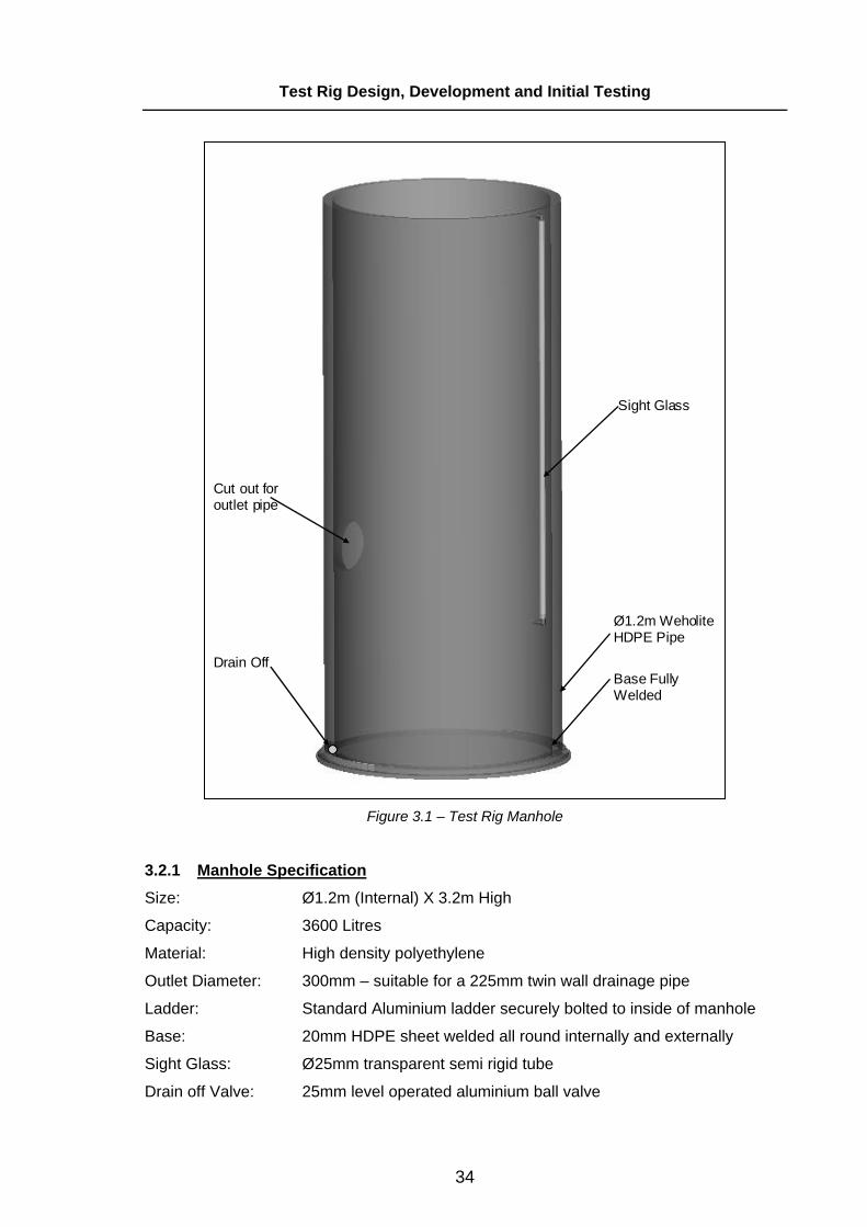
Figure 3.1 – Test Rig Manhole
3.2.1 Manhole Specification Size: Ø1.2m (Internal) X 3.2m High
Capacity: 3600 Litres
Material: High density polyethylene
Outlet Diameter: 300mm – suitable for a 225mm twin wall drainage pipe
Ladder: Standard Aluminium ladder securely bolted to inside of manhole
Base: 20mm HDPE sheet welded all round internally and externally
Sight Glass: Ø25mm transparent semi rigid tube
Drain off Valve: 25mm level operated aluminium ball valve

35
Test Rig Design, Development and Initial Testing
3.3 Flow Measurement Device and Water Holding Tank There were three main options available when choosing a method of measuring the flow
exiting the manhole through the vortex flow control device.
• An open channel flow meter
• An ultrasonic flow meter
• Weighing the volume of water exiting the system over a known period of time.
After an initial investigation it was discovered that both the open channel flow meter and
the ultrasonic flow meter were very expensive and have a budget cost of between €2,000
and €4,500. The author had access to a suitable weighing scales and holding tank so the
option of weighing the volume of water exiting the system over a known period of time
was chosen.
Data logging software was purchased and connected to the control panel of the weighing
scales via a laptop computer, this allowed live readings of the weight of water (and
therefore capacity of water) to be taken. The flow rate is determined by weighing the water
that flows through the vortex valve over a set period of time. The weight in kg’s is the
capacity in litres (assuming a density of water of 1000kg/m³), this is then divided by the
number of seconds the test was run at a constant head height to give the flow rate in litres
per second.
2500 Litre Holding Tank
2,000 kg Weighing Scales
Figure 3.2 – Test Rig Holding Tank and Weighing Scales
3.3.1 Weighing Scales and Holding Tank Specification Holding Tank Size: Ø2.0m X 0.8m
Capacity: 2500 Litres
Material: High density polyethylene
Weighing Scale Size: 1.5m X 1.5m X 0.15m
Weighing Scale Max Reading: 2,000kgs
Weighing Scale Increments: 0.01kgs

36
Test Rig Design, Development and Initial Testing
3.4 Water Supply to Manhole
There were two main options available to get a water supply into the manhole:
a) To pump water in from a reservoir tank.
b) To gravity feed water into the manhole from a header tank
The main constraint was the maximum flow rate at which the water would enter the
manhole and for what duration. The maximum flow rate into the manhole would have to
be greater than the maximum flow exiting the manhole from the vortex valve on test. The
maximum flow capability of the test rig would be limited by the physical size of the pipe
work entering the tank and the pressure from the water source.
Both options available were capable of delivering large flow rates with the pumped options
the most suitable because of the consistent flow rate. The main decision in choosing
either the pumped or gravity fed options was based on cost. A cost comparison was
carried out on each option as seen in table 3.1 below.
Components Pumped Option Header Tank Option
Cost Cost
Pump with 15l/s outlet €1,650and head of 3.5m100mm Pipe work for Pump €125
Header Tank And Frame €300Standard Support Frame €150Custom Support Frame €100Pipes & Fittings €150Pump to fill header tank €650
Total Cost €1,775 €1,350 Table 3.1 – Cost Comparison on Water Supply
It can be seen that the pumped option is more expensive than the header tank by €425,
the pumped option is the preferred option but due to cost constraints the header tank
option was selected. The header tank is a 2,000 litre plastic tank with a steel support
frame, this was installed on top of another standard support frame and a custom support
frame to lift the exit of the header tank to a point above the top of the manhole. A 100mm
PVC pipe was used to connect the exit of the header tank to the manhole. See assembly
section for more details.
The maximum flow rate from the header tank was expected to be between 10-20 l/s
depending on the head of water in the tank and efficiency losses through the pipe work.
37
Test Rig Design, Development and Initial Testing
3500 Litre Holding Tank
Standard Steel Support Frame
Standard Steel Support Frame
Custom Steel Support Frame
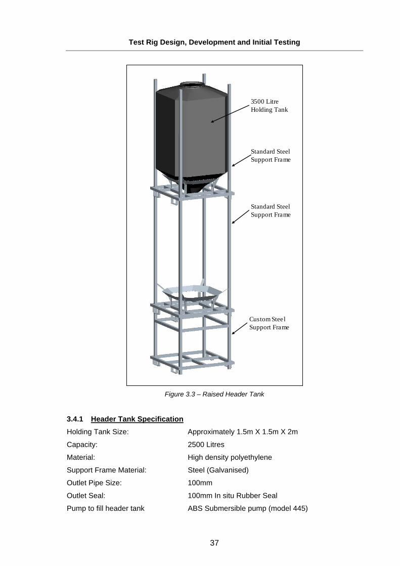
Figure 3.3 – Raised Header Tank
3.4.1 Header Tank Specification Holding Tank Size: Approximately 1.5m X 1.5m X 2m
Capacity: 2500 Litres
Material: High density polyethylene
Support Frame Material: Steel (Galvanised)
Outlet Pipe Size: 100mm
Outlet Seal: 100mm In situ Rubber Seal
Pump to fill header tank ABS Submersible pump (model 445)
38
Test Rig Design, Development and Initial Testing
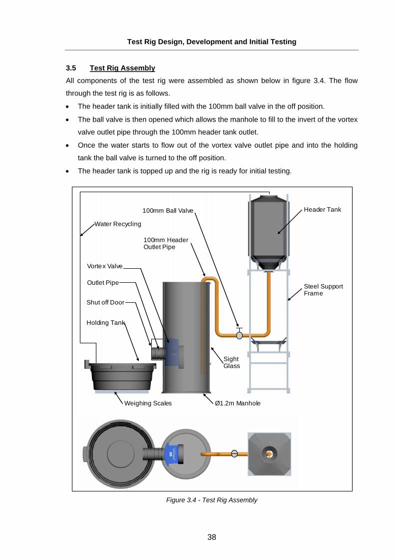
3.5 Test Rig Assembly All components of the test rig were assembled as shown below in figure 3.4. The flow
through the test rig is as follows.
• The header tank is initially filled with the 100mm ball valve in the off position.
• The ball valve is then opened which allows the manhole to fill to the invert of the vortex
valve outlet pipe through the 100mm header tank outlet.
• Once the water starts to flow out of the vortex valve outlet pipe and into the holding
tank the ball valve is turned to the off position.
• The header tank is topped up and the rig is ready for initial testing.
Vortex Valve
Shut off Door
Holding Tank
100mm Header Outlet Pipe
100mm Ball Valve
Weighing Scales
Header Tank
Steel Support Frame
Ø1.2m Manhole
Sight Glass
Water Recycling
Outlet Pipe
Figure 3.4 - Test Rig Assembly

39
Test Rig Design, Development and Initial Testing
Figure 3.5 – Photographs of Test Rig
40
Test Rig Design, Development and Initial Testing
3.6 Test Procedure
The test procedure was designed to calculate the flow rate from the vortex valve at head
heights incrementing from 0 to 2000mm in steps of 100mm. By combining and graphing
all these flow rates and head heights the performance characteristic of the vortex valve
can be generated.
The following steps were carried out in sequence to test the performance curve of a vortex
valve:
• Fill the header tank fully and fill the manhole to the point where water starts to exit
the outlet pipe i.e. zero head.
• Fill the holding tank with 100mm of water. This removes any fluctuations in the
weighing scale readings associated with the water falling from the outlet pipe into
the holding tank.
• Open the ball valve allowing water flow into the manhole through the vortex valve
and into the holding tank.
• Once the water reaches a head height of 100mm adjust the ball valve and keep
the head height constant.
• The recording equipment connected to the weighing scales was activated to
record the weight every 2 seconds over a period of 30 seconds. This gave an
accurate account of the volume of water that passed through the valve over that
time period at a constant head height.
• The flow rate at that particular head height was calculated by dividing the change
in mass of the tank in kg’s by the duration of the test in seconds. This gave mass
flow rate in kg/s and therefore l/s assuming a density of 1000 kg/m³ for water.
• The holding tank was pumped into the header tank and topped up as required
from a water hose until the tank was full again.
• The head height was increased to 200mm and the procedure repeated until the
mass flow rate was obtained.
• This test was carried out at increments of 100mm between 0 and 2000mm.
• All the test results were plotted in a graph of head height vs. flow rate to give the
performance characteristic of the valve.

41
Test Rig Design, Development and Initial Testing
3.7 Test Rig Performance Test It was necessary to establish the maximum flow rate that could be passed through the test
rig before initial prototype geometry was selected. A simple test was carried out as
follows:
• A vortex valve mounting adaptor was attached to the inside of the manhole with no
vortex chamber assembly. (This allowed unrestricted flow through to the holding
tank)
• The header tank was filled and the manhole sump primed (therefore when the ball
valve is opened water will flow into the holding tank)
• The 100mm ball valve is opened until there is approximately 200mm of water in
the holding tank.
• The header tank is refilled from an external water source.
• The weighing scales is set to zero.
• The 100mm ball valve is fully opened for 30 seconds and shut off.
• A reading is taken from the weighing scales of 377.25kgs.
• 377.25kg / 30 sec = 12.575 kg/s = 12.575 l/s.
• An approximate maximum flow rate of 12.5l/s was obtained for the test rig.
3.8 Initial Vortex Valve Prototype Geometry An initial prototype geometry was developed to require a maximum flow rate of less than
12l/s. An overall swirl diameter of 350mm was arbitrarily selected, an outlet diameter of
100mm was again arbitrarily selected as a starting outlet diameter. The inlet height and
width of the unit of 88mm was selected as this provided approximately the same inlet and
outlet cross sectional area.
Figure 3.6 - Initial Prototype
W
OD
H1
SD
SD = Swirl Diameter (Internal) (350mm)
OD = Orifice diameter (Outlet) (100mm)
W = Width (Internal) (88mm)
H1 = Height (Internal) (88mm)
42
Test Rig Design, Development and Initial Testing
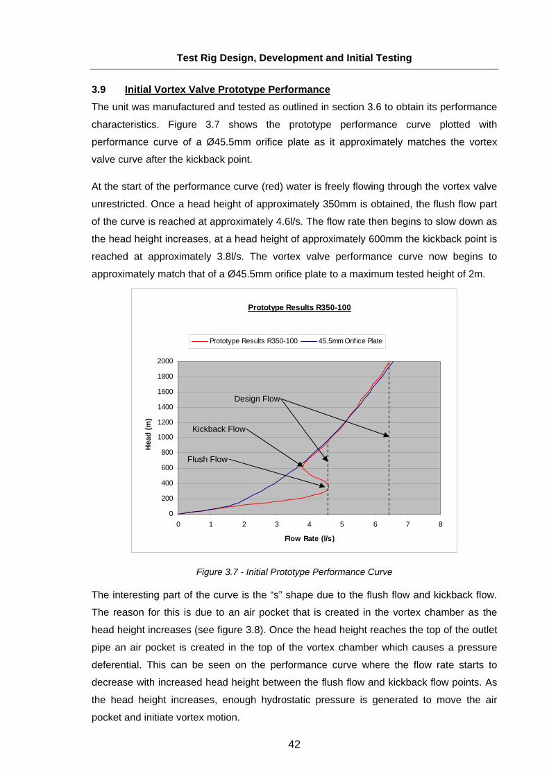
3.9 Initial Vortex Valve Prototype Performance The unit was manufactured and tested as outlined in section 3.6 to obtain its performance
characteristics. Figure 3.7 shows the prototype performance curve plotted with
performance curve of a Ø45.5mm orifice plate as it approximately matches the vortex
valve curve after the kickback point.
At the start of the performance curve (red) water is freely flowing through the vortex valve
unrestricted. Once a head height of approximately 350mm is obtained, the flush flow part
of the curve is reached at approximately 4.6l/s. The flow rate then begins to slow down as
the head height increases, at a head height of approximately 600mm the kickback point is
reached at approximately 3.8l/s. The vortex valve performance curve now begins to
approximately match that of a Ø45.5mm orifice plate to a maximum tested height of 2m.
Figure 3.7 - Initial Prototype Performance Curve
The interesting part of the curve is the “s” shape due to the flush flow and kickback flow.
The reason for this is due to an air pocket that is created in the vortex chamber as the
head height increases (see figure 3.8). Once the head height reaches the top of the outlet
pipe an air pocket is created in the top of the vortex chamber which causes a pressure
deferential. This can be seen on the performance curve where the flow rate starts to
decrease with increased head height between the flush flow and kickback flow points. As
the head height increases, enough hydrostatic pressure is generated to move the air
pocket and initiate vortex motion.
Prototype Results R350-100
0
200
400
600
800
1000
1200
1400
1600
1800
2000
0 1 2 3 4 5 6 7 8
Flow Rate (l/s)
Hea
d (m
)
Prototype Results R350-100 45.5mm Orif ice Plate
Flush Flow
Kickback Flow
Design Flow

43
Test Rig Design, Development and Initial Testing
Air Pocket
Figure 3.8 – Air Pocket on Vortex Chamber
The characteristics of the unit were found to be the following:
Swirl Diameter (Internal) (350mm)
Orifice diameter (Outlet) (100mm)
Width (Internal) (88mm)
Height (Internal) (88mm)
Design Flow: 4.6 – 6.41 l/s depending on head height
Flush Flow: 4.6 l/s
Kickback flow: 3.8 l/s
Corresponding Orifice Plate Diameter after Kickback Point: Ø45.5mm
CSA or Vortex Valve Outlet vs. CSA or Orifice Plate Outlet: Vortex Valve 4.8 times larger

44
Chapter 4
Detailed Testing, Modelling and CFD
4.0 Introduction Following on from the initial prototype testing in the last chapter, a series of tests were
carried out to determine the influence of each of the main geometric variables on the
performance of the vortex valve. The following geometric variables were varied
individually:
a) Outlet opening diameter
b) Width of the vortex valve
c) Inlet height of the vortex valve
d) Overall Swirl Diameter
From the results of the testing a relationship was chosen between each of the geometric
variables based on the following objectives:
1. Outlet opening diameter to have a cross sectional area 3 – 6 times that of the
opening on an orifice plate of the same specification.
2. Inlet and outlet opening to be of similar size to minimise the possibility of a
blockage when in service.
3. The distance between the kickback point and the flush flow point along the X axis
is to be minimised to allow the design flow to be reached at lower head heights.
4. “Area A” is to be maximised while keeping the kickback line as close to vertical as
possible (see figure 4.1 below). This will maximise the flow through the vortex
valve as the head height increases.
Typical Performance Curve
0
2 00
4 00
6 00
8 00
1 000
1 2 00
1 4 00
1 6 00
1 8 00
2 000
0 2 4 6 8
Flow (l/s)
Hea
d (m
m)
Area A Kickback Line
Flush Flow Point
Kickback Point
Head
(mm
)
Flow Rate (l/s)
Figure 4.1 – Area A on Typical Performance Curve

45
Detailed Testing, Modelling and CFD
4.1 Varying the Vortex Valve Outlet Diameter Following the initial prototype testing, four more units were manufactured with the same
geometry as the initial prototype except for the outlet orifice diameter. Two units were
manufactured with larger openings and two with smaller openings as outlined below. Each
unit was individually tested to establish the relationship between the diameter of the outlet
orifice and the flow curve of the unit. The following orifice diameters were tested:
Unit 1 – Outlet Orifice Ø50mm
Unit 2 – Outlet Orifice Ø75mm
Unit 3 – Outlet Orifice Ø100mm (initial prototype)
Unit 4 – Outlet Orifice Ø125mm
Unit 5 – Outlet Orifice Ø150mm
R350 Outlet Diameter Comparison
0
200
400
600
800
1000
1200
1400
1600
1800
2000
0 2 4 6 8 10
Flow (l/s)
Hea
d (m
m)
R350-Ø50 R350-Ø75 R350-Ø100 R350-Ø125 R350-Ø150
Figure 4.2 – Varying the Outlet Diameter
The performance curve of each of the five units tested are plotted in figure 4.2 above, the
flow capacity of each unit increases as the outlet opening diameter is increased. It can be
seen that as the outlet opening diameter increases the kickback and flush flow point of the
curve decreases. The distance between the flush flow and kickback flow points also
decreases as the outlet opening diameter is increased. The design flow region of the
curve shows a large increase as the outlet opening diameter is increased.

46
Detailed Testing, Modelling and CFD
4.1.1 Satisfying Design Objectives
The first objective was for the vortex valve outlet cross sectional area to be 3 – 6 times
larger than a corresponding orifice plate to minimise blockages. It can be seen from table
4.1 that it needs to be a minimum of 75mm in diameter to satisfy this constraint (Curve 2). Vortex Valve Vortex Valve Corresponding Corresponding CSA
Outlet Diameter CSA Orifice Plate Diameter Orifice Plate CSA Difference(mm) (mm²) (mm) (mm²) (times)
50 1,963 38 1,134 1.7375 4,416 42.5 1,418 3.11100 7,850 45.5 1,625 4.83125 12,266 50.5 2,002 6.13150 17,663 54.5 2,332 7.58
Table 4.1 – Cross Sectional Area Analysis
The data above in table 4.1 was plotted below in figure 4.3. It can be seen that as the
vortex valve outlet opening diameter increases, the corresponding orifice plate diameter to
achieve the same specification above the kickback point increases in an approximately
linear fashion.
Relationship Between Vortex Valve Outlet Opening Diameterand Corresponding Orifice Plate Diameter
30
50
70
90
110
130
150
170
35 40 45 50 55Orifice Plate Diameter Diameter (mm)
Out
let O
peni
ng D
iam
eter
(mm
)
Actual Relatioship
Figure 4.3 – Outlet Diameter and Orifice Plate Relationship
The third objective is best satisfied by the largest vortex valve outlet opening diameter
(Ø150mm – Curve 5) in that its design flow range starts at the lowest head height. The
fourth objective is best satisfied by curve 3 with the Ø100mm outlet as after this point
“area A” begins to decrease. The best curve that satisfies all constraints is curve 3 with
the Ø100mm outlet opening diameter.

47
Detailed Testing, Modelling and CFD
4.1.2 Relationship Analysis
A relationship analysis was carried out to determine if the kickback part of the
performance curve could be linearly modelled as the outlet opening diameter is increased.
This information will be then used in deciding the best way to build a model to predict the
performance curve under a given specification.
The effect of the increased outlet opening diameter on the flush flow point and the
kickback flow point is shown in figure 4.4 below. As the outlet opening diameter increases
so does the flush flow point and kickback flow point, both increase the flow rate at different
rates but they both can be linearly approximated.
Relationship Between Vortex Valve Outlet Opening Diameterand Corresponding Kickback and Flush Flow Points
40
60
80
100
120
140
160
2.25 2.75 3.25 3.75 4.25 4.75 5.25
Flow (l/s)
Out
let O
peni
ng D
iam
eter
(mm
)
Flush Flow Kickback Flow
Figure 4.4 – Outlet Diameter and Flow Relationship
It can be seen below in figure 4.5 that as the outlet opening diameter increases the head
height required to reach the kickback flow point decreases. This is because with the larger
orifice opening there is less of an air pocket trapped in the top of the vortex valve thus
requiring less hydrostatic pressure to initiate the vortex (see figure 3.8). The kickback flow
is approximately linear between outlet opening diameters of Ø70mm and Ø120mm with
the flush flow approximately linear between Ø50mm and Ø120mm.

48
Detailed Testing, Modelling and CFD
Relationship Between Vortex Valve Outlet Opening Diameterand Corresponding Kickback and Flush Flow Head Heights
40
60
80
100
120
140
160
300 350 400 450 500 550 600 650 700 750
Head Height (mm)
Out
let O
peni
ng (m
m)
Kickback Flow Flush Flow
Figure 4.5 – Outlet Opening Diameter and Head Relationship
4.1.3 Summary of Increasing Vortex Valve Outlet Opening Diameter
The outlet opening diameter was increased from 50mm to 150mm in increments of 25mm.
The following conclusions were made on the effect of the increase on the performance
curve of the unit.
• Linearly increases the flow allowed to pass through the unit
• Linearly increases the kickback and flush flow point in flow axis
• Linearly decreases the kickback and flush flow point in head height axis
• Curve 3 with an outlet opening diameter of Ø100mm best satisfies all design
objectives as set out in section 4.0.

49
Detailed Testing, Modelling and CFD
4.2 Varying Vortex Valve Width The initial prototype was again used as the base geometry, all variables were kept
constant apart from the internal width of the unit as outlined below.
OD = Orifice diameter (Outlet) (100mm)
SD = Swirl Diameter (Internal) (350mm)
W = Width (Internal) (75,100,125,150,175mm)
H = Inlet Height (Internal) (88mm)
R350 Variable Width Analysis
0
200
400
600
800
1000
1200
1400
1600
1800
2000
0 2 4 6 8 10 12
Flow (l/s)
Hea
d (m
m)
R350-W75 R350-W100 R350-W125 R350-W150 R350-W175
Figure 4.6 – Varying the Width of the Vortex Valve
The performance curve of each of the five units tested are plotted in figure 4.6 above, the
flow capacity of each unit increases as the width of the vortex valve is increased. It can be
seen that increasing the width of the vortex valve from 75mm to 175mm increases the
flow by 4-7l/s. Increasing the width also increases the kickback point of the curve and
moves the kickback line of the curve to a more horizontal position. As the width is
increased it also increases the head height required to reach the kickback and flush flow
points.

50
Detailed Testing, Modelling and CFD
4.2.1 Satisfying Design Objectives
The first objective was for the vortex valve outlet cross sectional area to be 3 -6 times
larger than a corresponding orifice plate to minimise blockages. It can be seen from table
4.2 that it can be up to a maximum of 150mm in width to satisfy this constraint. Vortex Valve Vortex Valve Corresponding Corresponding CSA
Width Outlet CSA Orifice Plate Diameter Orifice Plate CSA Difference(mm) (mm²) (mm) (mm²) (times)
75 7,850 42.5 1,418 5.54100 7,850 47.75 1,790 4.39125 7,850 52 2,123 3.70150 7,850 56 2,462 3.19175 7,850 61.5 2,969 2.64
Table 4.2 – Width Analysis
The data above in table 4.2 was plotted below in figure 4.7. It can be seen that as the
vortex valve width is increased the corresponding orifice plate diameter to achieve the
same specification above the kickback point increases in an approximately linear fashion.
Relationship Between Width of Vortex Valveand Corresponding Orifice Plate Diameter
40
60
80
100
120
140
160
180
200
40 45 50 55 60 65
Corresponding Orifice Plate Diameter (mm)
Wid
th o
f Vor
tex
Valv
e (m
m)
Actual Relatioship
Figure 4.7 – Vortex Valve Width and Orifice Plate Relationship
The second objective is best satisfied by curve 2 at a width of 100mm.The third objective
is best satisfied by the smallest width vortex chamber at 75mm because its design flow
range starts at the lowest head height. The fourth objective is best satisfied by the largest
width vortex valve at 175mm but it has a big disadvantage due to the high head height
required to reach the design flow range. The curve that best satisfies all objectives is
curve 2 with a width of 100mm.

51
Detailed Testing, Modelling and CFD
4.2.2 Relationship Analysis
A relationship analysis was carried out to determine if the kickback part of the
performance curve could be linearly modelled as the width of the vortex chamber is
increased. This information will be then used in deciding the best way to build a model to
predict the performance curve under a given specification.
The effect of the increased width on the flush flow point and the kickback flow point is
shown in figure 4.8 below. As the width increases so does the flush flow at an
approximately linear rate after 4.5l l/s. The kickback flow increases at a different rate but
can be seen to be approximately linear throughout.
Relationship Between Width of Vortex Valveand Corresponding Kickback and Flush Flow Points
60
80
100
120
140
160
180
200
2.5 3.5 4.5 5.5 6.5 7.5 8.5 9.5 10.5
Flow (l/s)
Wid
th o
f Vor
tex
Valv
e (m
m)
Flush Flow Kickback Flow
Figure 4.8 – Outlet Diameter and Flow Relationship
As the outlet opening diameter increases the head height required to reach the kickback
flow and flush flow points increases. This is because with the larger width vortex valve
there is more of an air pocket trapped in the top of the vortex valve thus requiring more
hydrostatic pressure to initiate the vortex (see figure 3.8). It can be seen from figure 4.9
they increase in a non linear fashion.

52
Detailed Testing, Modelling and CFD
Relationship Between Width of Vortex Valveand Corresponding Kickback and Flush Flow Head Heights
50
70
90
110
130
150
170
190
350 400 450 500 550 600 650 700 750
Head Height (mm)
Wid
th o
f Vor
tex
Valv
e (m
m)
Flush Flow Kickback Flow
Figure 4.9 – Width and Orifice Plate Relationship
4.2.3 Summary of Increasing Width of Vortex Valve
The width of the vortex valve was increased from 75mm to 175mm in increments of
25mm. The following conclusions were made on the effect of the increase in the width of
the vortex valve.
• Linearly increases the flow allowed to pass through the unit after the kickback
point
• Linearly increases the kickback and flush flow point in the flow axis
• Non-linearly increases the kickback and flush flow point in head height axis
• Curve 2 with a width of Ø100mm best satisfies all design objectives as set out in
section 4.0.
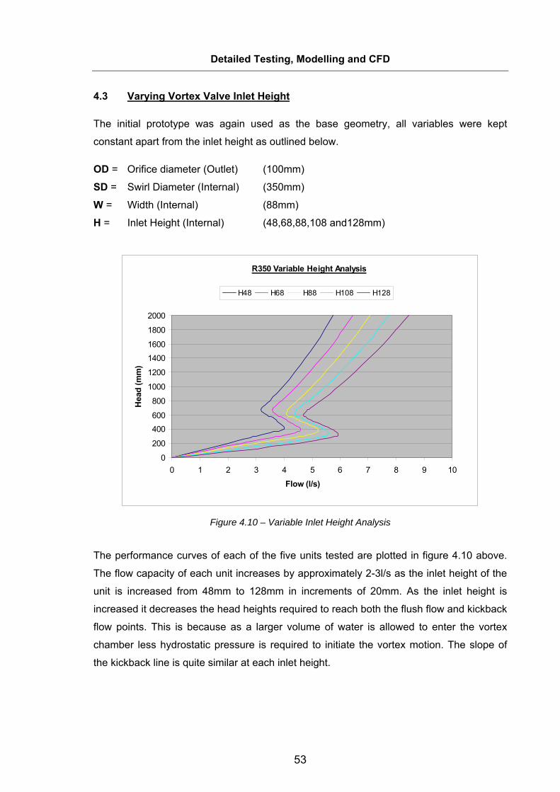
53
Detailed Testing, Modelling and CFD
4.3 Varying Vortex Valve Inlet Height
The initial prototype was again used as the base geometry, all variables were kept
constant apart from the inlet height as outlined below.
OD = Orifice diameter (Outlet) (100mm)
SD = Swirl Diameter (Internal) (350mm)
W = Width (Internal) (88mm)
H = Inlet Height (Internal) (48,68,88,108 and128mm)
R350 Variable Height Analysis
0
200
400600
800
1000
1200
1400
1600
1800
2000
0 1 2 3 4 5 6 7 8 9 10
Flow (l/s)
Hea
d (m
m)
H48 H68 H88 H108 H128
Figure 4.10 – Variable Inlet Height Analysis
The performance curves of each of the five units tested are plotted in figure 4.10 above.
The flow capacity of each unit increases by approximately 2-3l/s as the inlet height of the
unit is increased from 48mm to 128mm in increments of 20mm. As the inlet height is
increased it decreases the head heights required to reach both the flush flow and kickback
flow points. This is because as a larger volume of water is allowed to enter the vortex
chamber less hydrostatic pressure is required to initiate the vortex motion. The slope of
the kickback line is quite similar at each inlet height.

54
Detailed Testing, Modelling and CFD
4.3.1 Satisfying Design Objectives
The first objective was for the vortex valve outlet cross sectional area to be 3 -6 times
larger than a corresponding orifice plate to minimise blockages. It can be seen from table
4.3 that it needs to be a minimum of 75mm in diameter to satisfy this constraint (Curve 2). Inlet Height Vortex Valve Corresponding Corresponding CSA
Outlet CSA Orifice Plate Diameter Orifice Plate CSA Difference(mm) (mm²) (mm) (mm²) (times)
48 7,850 43 1,451 5.4168 7,850 45.5 1,625 4.8388 7,850 47.5 1,771 4.43108 7,850 50 1,963 4.00128 7,850 52 2,123 3.70
Table 4.3 – Inlet Height Analysis
The data above in table 4.3 was plotted below in figure 4.11. It can be seen that as the
vortex valve inlet height is increased the corresponding orifice plate diameter to achieve
the same specification above the kickback point increases in an approximately linearly
fashion.
Relationship Between Inlet Height of Vortex Valveand Corresponding Orifice Plate Diameter
405060708090
100110120130140
40 42 44 46 48 50 52 54Corresponding Orifice Plate Diameter (mm)
Inle
t Hei
ght (
mm
)
Actual Relatioship
Figure 4.11 – Vortex Valve Inlet Height and Orifice Plate Relationship
The second objective is best satisfied by the inlet height of 108mm. The third objective is
best satisfied by the inlet height at 48mm but it can be seen that increasing the inlet height
has little effect on the design flow range when compared with the two previous variables.
The fourth objective is best satisfied by the largest inlet height at 128mm. The inlet height
that best satisfies all constraints is 88mm.
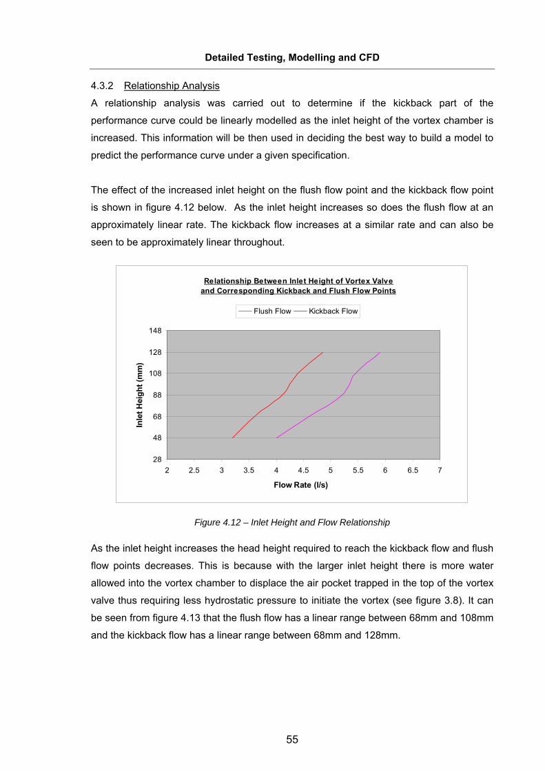
55
Detailed Testing, Modelling and CFD
4.3.2 Relationship Analysis
A relationship analysis was carried out to determine if the kickback part of the
performance curve could be linearly modelled as the inlet height of the vortex chamber is
increased. This information will be then used in deciding the best way to build a model to
predict the performance curve under a given specification.
The effect of the increased inlet height on the flush flow point and the kickback flow point
is shown in figure 4.12 below. As the inlet height increases so does the flush flow at an
approximately linear rate. The kickback flow increases at a similar rate and can also be
seen to be approximately linear throughout.
Relationship Between Inlet Height of Vortex Valveand Corresponding Kickback and Flush Flow Points
28
48
68
88
108
128
148
2 2.5 3 3.5 4 4.5 5 5.5 6 6.5 7
Flow Rate (l/s)
Inle
t Hei
ght (
mm
)
Flush Flow Kickback Flow
Figure 4.12 – Inlet Height and Flow Relationship
As the inlet height increases the head height required to reach the kickback flow and flush
flow points decreases. This is because with the larger inlet height there is more water
allowed into the vortex chamber to displace the air pocket trapped in the top of the vortex
valve thus requiring less hydrostatic pressure to initiate the vortex (see figure 3.8). It can
be seen from figure 4.13 that the flush flow has a linear range between 68mm and 108mm
and the kickback flow has a linear range between 68mm and 128mm.

56
Detailed Testing, Modelling and CFD
Relationship Between Inlet Height of Vortex Valveand Corresponding Kickback and Flush Flow Head Heights
28
48
68
88
108
128
148
300 350 400 450 500 550 600 650 700 750 800
Head Height (mm)
Inle
t Hei
ght (
mm
)
Flush Flow Kickback Flow
Figure 4.13 – Inlet Height and Head Height Relationship
4.3.3 Summary of Increasing Inlet Height of Vortex Valve The inlet height of the vortex valve was increased from 48mm to 128mm in increments of
20mm. The following conclusions were made on the effect of the increase in the inlet
height of the vortex valve.
• Linearly increases the flow allowed to pass through the unit after the kickback
point
• Linearly increases the kickback and flush flow points in the flow axis
• Non-linearly decreases the kickback and flush flow point in head height axis
• Curve 2 with an inlet height of 88mm best satisfies all design objectives as set out
in section 4.0.

57
Detailed Testing, Modelling and CFD
4.4 Establishing the Relationship between Geometric Variables
Varying the swirl diameter of the vortex valve was not carried out independently of the
other variables as with the previous comparisons. The swirl diameter is the largest
geometric variable and will therefore have the largest effect on flow rate. It is the main
variable that changes in commercial vortex valves and it was decided to select a
relationship between each of the other variables and scale the overall geometry as the
swirl diameter was increased / decreased.
4.4.1 Outlet Opening Diameter
The outlet opening diameter was constrained by the fact that its CSA was required to be
3-6 times that or a corresponding orifice. Therefore an outlet opening diameter between
75mm and 125mm will satisfy that objective. All objectives are best satisfied using an
outlet opening diameter of approximately 100mm as can be seen in section 4.1. The exact
size is determined in conjunction with the width of the vortex valve as outlined below in
section 4.4.2.
4.4.2 Width of the Vortex Valve
The width of the vortex valve was constrained by the outlet opening diameter as the inlet
and outlet openings were required to be of similar size to minimise blockage during
service. Therefore it was decided to make the width of the vortex valve and the outlet
opening diameter the same size. A ratio of 4:1 between the swirl diameter, and both the
outlet opening diameter and the width of the vortex valve will give a size of 88mm. This in
turn provides an outlet opening diameter with a CSA 4 times greater than the
corresponding orifice plate satisfying the first objective.
4.4.3 Inlet Height of the Vortex Valve
The inlet height of the vortex valve was constrained by both the outlet opening diameter
and the width of the vortex valve. To minimise blockages in service the inlet height was
set equal to both the width and outlet opening diameter at a ratio of 4:1 with the swirl
diameter.

58
Detailed Testing, Modelling and CFD
4.5 Varying the Swirl Diameter The effect of increasing / decreasing the swirl diameter was investigated by testing six
units with swirl diameters between 200mm and 450mm in increments of 50mm. The
relationship between the swirl diameter and the other geometric variables established in
the previous section was used on all units.
SD = Swirl Diameter (Internal) (200, 250, 300, 350, 400, 450mm)
OD = Orifice diameter (Outlet) (swirl diameter / 4)
W = Width (Internal) (swirl diameter / 4)
H1 = Height (Internal) (swirl diameter / 4)
Figure 4.14 – Prototype Geometry
The performance curve of each of the six units tested are plotted in figure 4.15 below, the
flow capacity of each unit increases by approximately 7 l/s as the swirl diameter is
increased between 200m and 450mm. Figure 4.15 also shows that as the swirl diameter
is increased it increases both the flush flow and kickback flow points. It also increases the
head height required to reach the flush flow and kickback flow points because of the extra
hydrostatic pressure required to move the air pocket and initiate the vortex.
W
OD
H1
SD

59
Detailed Testing, Modelling and CFD
Effects on Increasing the Swirl Diameter
0
200
400
600
800
1000
1200
1400
1600
1800
2000
0 1 2 3 4 5 6 7 8 9 10
Flow (l/s)
Head
Hei
ght (
m)
R200-50 R250-62.5 R300-75 R350-88 R400-100 R450-112.5
Figure 4.15 – Varying the Swirl Diameter
4.5.1 Relationship Analysis
A relationship analysis was carried out to determine if the performance of the units
increased at a linear rate as the swirl diameter is increased. This information will be then
used in deciding the best way to build a model to predict the performance curve under a
given specification.
The relationship between the swirl diameter of the vortex valve and the corresponding
orifice plate diameter of the same specification can be seen below in figure 4.16. It shows
a linear relationship between the two in the region of the performance curve above the
kickback flow point. Therefore if the orifice plate diameter is known for a specific flow
specification, the corresponding vortex valve swirl diameter and therefore the complete
vortex valve geometry can be determined.
The effect of the increased swirl diameter on the flush flow point and the kickback flow
point is shown in figure 4.17 below. As the swirl diameter increases so does the flush flow
and kickback flow at a non linear rate.

60
Detailed Testing, Modelling and CFD
Relationship Between Swirl Diameter and Corresponding Orifice Plate Diameter
150
200
250
300
350
400
450
500
20 25 30 35 40 45 50 55 60
Orifice Plate Diameter (mm)
Sw
irl D
iam
eter
(mm
)Relationship
Figure 4.16 – Swirl Diameter and Orifice Plate Relationship
Relationship Between Swirl Diameter andCorresponding Flush / Kickback Flow Rates
0
100
200
300
400
500
600
0 1 2 3 4 5 6 7 8 9
Flow Rate (l/s)
Sw
irl D
iam
eter
(mm
)
Kickback Flow Flush Flow
Figure 4.17 – Swirl Diameter and Flush Flow / Kickback Flow Relationship

61
Detailed Testing, Modelling and CFD
Relationship Between Swirl Diameter andCorresponding Flush / Kickback Head Height
0
100
200
300
400
500
600
100 200 300 400 500 600 700 800 900
Head Height (mm)
Swirl
Dia
met
er (m
m)
Flush Kickback
Figure 4.18 – Swirl Diameter and Flush Flow / Kickback Flow Head
The effect of the increased swirl diameter on the head height required to reach the flush
flow point and the kickback flow point is shown in figure 4.18 above. As the swirl diameter
increases so does the flush flow and kickback flow at an approximately linear rate.
4.5.2 Summary of Increasing Swirl Diameter of Vortex Valve
The swirl diameter was increased from 200mm to 450mm in increments of 50mm. Each of
the other variables were scaled up as appropriate to give the same geometric relationship.
The following conclusions were made on the effect of the increase in the swirl diameter of
the vortex valve.
• Linearly increases the flow allowed to pass through the unit after the kickback
point
• Non-linearly increases the kickback and flush flow points in the flow axis
• Approximately linearly increases the head height required to reach the kickback
and flush flow points.

62
Detailed Testing, Modelling and CFD
4.6 Vortex Valve Geometry Modelling An important feature of any vortex valve design is the ability to accurately predict it’s
geometric dimensions for any given specification without the need for testing individual
units. For example, if a specific design required a flow rate of 6l/s at a head height of
1000mm what is the geometry of the unit required? A model was built from the results
obtained during the full scale testing as follows.
• A linear relationship was established between the performance of the vortex valve
at a given swirl diameter and a corresponding orifice plate at the same flow
specification as detailed in section 4.5.1.
• Using the formula for discharge through a small orifice [18], the orifice plate
diameter can be determined from a specific flow rate and head height i.e.
specification of the vortex valve.
• Insert this orifice plate diameter into the linear equation obtained from figure 4.19
below (y=9.2389x – 45.709) to provide an equivalent vortex valve swirl diameter.
• The swirl diameter is then divided by four to find the width, inlet height and outlet
opening diameter as outlined in section 4.4
Relationship Between Swirl Diameter and Corresponding Orifice Plate Diameter
y = 9.2389x - 45.709
150
200
250
300
350
400
450
500
20 25 30 35 40 45 50 55 60
Orifice Plate Diameter (mm)
Swirl
Dia
met
er (m
m)
Relationship Linear (Relationship)
Figure 4.19 – Linear Equation Swirl Diameter and Orifice Plate Relationship
63
Detailed Testing, Modelling and CFD
4.6.1 Example: Required Design Flow = 6l/s
Required Design Head = 1000mm
Formula for Flow through a small Orifice:
Q = CD x A x √2gh [18] Q = Flow in cubic meters per second (m³/s)
A = CSA of the orifice diameter in meters (m)
G = Acceleration due to gravity (m²/s)
H = Head Height in meters (m)
CD = Coefficient of Discharge (0.65)
0.006 = .65 X A X √(2 X 9.81 X 1)
0.006 = A X 2.879
A = 0.00208406 m²
r² = 0.000663m
r = 0.02576m
Orifice Plate Diameter = 0.0515m = 51.5mm
Substituting this value for “x” in the formula given in figure 4.26 = 430.1mm
Swirl diameter = 430.1mm
Outlet Opening Diameter = 430 / 4 = 107.5mm
Width = 430 / 4 = 107.5mm
Inlet Height = 430 / 4 = 107.5mm

64
Detailed Testing, Modelling and CFD
4.7 Vortex Valve Performance Curve Modelling There are two ways in which the performance curve of a specific geometry can be
modelled, both methods offer individual advantages and disadvantages.
4.7.1 Unique Swirl Diameter Vortex Valves
Using a unique swirl diameter for each individual specification enables the relationship
between all geometric variables to be kept constant. Therefore increasing / decreasing the
overall size of the unit to the required dimensions as outlined in section 4.6 can be used to
give a specific performance. The model used to predict the vortex valve performance
curve using a unique swirl diameter was built as follows:
• A Microsoft excel calculator (see figure 4.20) was built from the data in
section 4.6 to predict the geometry of the vortex valve with a known
specification. (e.g. flow rate and head height)
Gravity (m/s) 9.810Head (mm) 1200.000Head Height (m) 1.200Coefficient of Discharge 0.650
Outlet Flow Rate (l/s) 4.5006.923
CSA of Orifice 5996.071Inlet Height 68.624sqrt 2 gh 4.852Q/sqrt 2 gh = (A) 0.001r sqrd 0.000r 0.021Orifice Diameter (mm) 42.62
Vortex Outlet Diameter (mm) 87.4Vortex Swirl Diameter (mm) 350Vortex Width (mm) 87.4Head (mm) 1200Desired Flow Rate (l/s) 4.5
Vortex Valve Calculator
Figure 4.20 – Vortex Valve Calculator
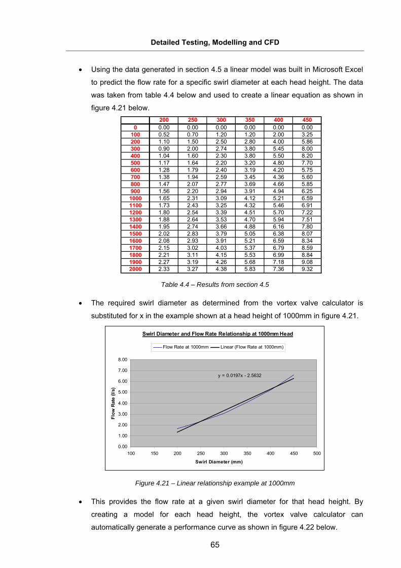
65
Detailed Testing, Modelling and CFD
• Using the data generated in section 4.5 a linear model was built in Microsoft Excel
to predict the flow rate for a specific swirl diameter at each head height. The data
was taken from table 4.4 below and used to create a linear equation as shown in
figure 4.21 below. 200 250 300 350 400 450
0 0.00 0.00 0.00 0.00 0.00 0.00100 0.52 0.70 1.20 1.20 2.00 3.25200 1.10 1.50 2.50 2.80 4.00 5.86300 0.90 2.00 2.74 3.80 5.45 8.00400 1.04 1.60 2.30 3.80 5.50 8.20500 1.17 1.64 2.20 3.20 4.80 7.70600 1.28 1.79 2.40 3.19 4.20 5.75700 1.38 1.94 2.59 3.45 4.36 5.60800 1.47 2.07 2.77 3.69 4.66 5.85900 1.56 2.20 2.94 3.91 4.94 6.251000 1.65 2.31 3.09 4.12 5.21 6.591100 1.73 2.43 3.25 4.32 5.46 6.911200 1.80 2.54 3.39 4.51 5.70 7.221300 1.88 2.64 3.53 4.70 5.94 7.511400 1.95 2.74 3.66 4.88 6.16 7.801500 2.02 2.83 3.79 5.05 6.38 8.071600 2.08 2.93 3.91 5.21 6.59 8.341700 2.15 3.02 4.03 5.37 6.79 8.591800 2.21 3.11 4.15 5.53 6.99 8.841900 2.27 3.19 4.26 5.68 7.18 9.082000 2.33 3.27 4.38 5.83 7.36 9.32
Table 4.4 – Results from section 4.5
• The required swirl diameter as determined from the vortex valve calculator is
substituted for x in the example shown at a head height of 1000mm in figure 4.21.
Swirl Diameter and Flow Rate Relationship at 1000mm Head
y = 0.0197x - 2.5632
0.00
1.00
2.00
3.00
4.00
5.00
6.00
7.00
8.00
100 150 200 250 300 350 400 450 500
Swirl Diameter (mm)
Flow
Rat
e (l/
s)
Flow Rate at 1000mm Linear (Flow Rate at 1000mm)
Figure 4.21 – Linear relationship example at 1000mm
• This provides the flow rate at a given swirl diameter for that head height. By
creating a model for each head height, the vortex valve calculator can
automatically generate a performance curve as shown in figure 4.22 below.

66
Detailed Testing, Modelling and CFD
Performance Curve of Vortex Valvewith Ø350mm Swirl Diameter
0
200
400
600
800
1000
1200
1400
1600
1800
2000
0.00 1.00 2.00 3.00 4.00 5.00 6.00 7.00
Flow (l/s)
Hea
d He
ight
(m)
R350-88
Figure 4.22 – Vortex Valve Calculator Generated Performance Curve
Advantages to the Unique Swirl Diameter model
• Accurate performance of a given specification can be determined above the flush
flow point.
• CSA of the vortex valve is always 4 times that of the corresponding orifice plate.
• Useful model if only interested in the design flow value.
Disadvantages to the Unique Swirl Diameter model
• Performance of the vortex valve before the kickback flow point cannot be
accurately predicted because of the non linear relationships. (see figure 4.17 and
4.18)
• The non linear relationships associated with the model around the flush flow and
kickback flow points means there will be inaccuracies with storage volume
calculations using the data from the model.
67
Detailed Testing, Modelling and CFD
4.7.2 Standard Swirl Diameters Vortex Valves
All the testing for this model was not carried out as part of the research due to time and
cost constraints but the results of section 4.1 and 4.5 show that it will accurately model the
performance curve within a specific range.
Using a standard range of vortex valve with set swirl diameters the units can be
customised to suit a specific performance requirement i.e. flow rate. Using the results from
section 4.1 it can be said there is a linear relationship between the performance curves of
the vortex valve as the outlet opening diameter is increased / decreased within a certain
range.
The range is determined as follows:
Minimum Orifice Diameter = Swirl Diameter / 5
Maximum Orifice Diameter = Swirl Diameter / 3
Therefore if a number of standard vortex valves sizes were built with the same geometric
relationship as outlined in section 4.6, it is possible to pick the nearest standard size swirl
diameter for a given specification and modify the outlet opening diameter to give the
specific performance required and accurately predict its performance curve.
As an example the following range may be selected.
Unit 1 – Swirl Diameter 200mm
Unit 2 – Swirl Diameter 250mm
Unit 3 – Swirl Diameter 300mm
Unit 4 – Swirl Diameter 350mm
Unit 5 – Swirl Diameter 400mm
Unit 6 – Swirl Diameter 450mm
In order for the linear relationship of the standard size vortex valves to be used each
vortex valve needs to be tested as follows:
• At normal outlet opening diameter (4:1 relationship)
• At maximum outlet diameter (swirl diameter / 3)
• At minimum outlet diameter (swirl diameter / 5)
Using the results of these tests a linear model can be built for the performance of that
specific vortex valve with varying outlet opening diameters.

68
Detailed Testing, Modelling and CFD
An example of the steps carried out to accurately model the performance curve using this
method is outlined below:
1. Using the method outlined in section 4.6 the required ideal geometric size of the
vortex valve can be determined.
2. The available range of vortex valves are analysed to match the desired swirl
diameter to the nearest standard size.
3. Using the Microsoft Excel model of that standard size vortex valve the design flow
rate was used as an input at the required head height. This then outputs a
corresponding outlet opening diameter and performance curve for that specific
standard size unit.
Advantages to using a Range of Set Swirl Diameters
• An accurate performance curve can be determined at all head heights.
• It optimises the manufacturing process of the vortex valves in a production
environment.
• The performance curve can be used to accurately calculate the required storage
volume of an attenuation system.
Disadvantages to using a Range of Standard Swirl Diameters
• The CSA of the outlet opening diameter changes depending on the required
specification.
4.8 Limitations Experienced During Testing
Two problems were identified during all the full scale testing:
1. The full scale test rig could not handle flow rates above 12l/s which was a
disadvantage in not being able to test larger size vortex valves with larger flow
rates.
2. The optimal relationship between the geometric variables as set out in section 4.4
requires very large vortex valves for flow above approximately 15-20l/s. Above this
rate the physical size of the vortex valve would make it difficult to install in a
standard Ø1.2m storm water manhole.
To identify a possible solution for these two problems it was decided to investigate if
computational fluid dynamics (CFD) could be used to simulate flow through the vortex
valve and evaluate its correlation with physical test results.

69
Detailed Testing, Modelling and CFD
4.9 Computational Fluid Dynamics
CFD was used to simulate fluid flow through the vortex valve, there are three main steps
in a CFD simulation using Ansys CFX software – 1) Pre-processing which includes
geometry creation, meshing, physics and numerics. 2) Solving and 3) Post-processing
[13]. Each stage is critical as incorrect assumptions or decisions made in developing the
model will lead to inaccuracies in the results. For this reason the model was developed
using experimental data for validation purposes.
4.9.1 Model Setup
Pre Processing - Geometry
A 3D modelling package called Pro Engineer was used to generate the geometry for the
analysis. A simplified representation of a vortex valve in a rectangular manhole was used
as can be seen in figure 4.23. The volume occupied by air / water in the manhole was
modelled for the simulation.
Pre-Processing – Meshing
The geometry created in Pro Engineer was transferred to Ansys CFX-Mesh, here the
geometry was broken down into regions. Similar surfaces were assembled together to
form regions. Specific meshing constraints were then applied to each region to give a high
quality mesh. Manhole Outlet
Walls PipeAngular Resolution (°)
15 30 15 30 15
Max. Edge Length (mm)
24 50 24 50 24
Min. Edge Length (mm)
8 10 8 10 8
Vortex Chamber
Manhole Opening (Top)
Outlet Pipe Opening
Table 4.5 – Mesh Settings
Advanced mesh inflation was used on boundary layers to give a more concentrated mesh
at surface / fluid interfaces. The following inflation and mesh settings were used on the
regions. Manhole Outlet
Walls PipeNo. of Inflated Layers 5 5 5
Expansion Factor 1.2 1.2 1.2
Min. internal angle (°) 2.5 2.5 2.5
Max. external angle (°) 10 10 10
Vortex Chamber
Table 4.6 – Advanced Mesh Settings

70
Detailed Testing, Modelling and CFD
Figure 4.23 – CFD Mesh
Mesh settings are a compromise of accuracy and computation time, these settings were optimized in the validation section to give an acceptable quality of result data and computation time. Surface meshes as shown in figure 4.23 were computed to volume meshed for use with the pre-processor in the setup of the physics model [20].
Pre-Processing – Physics and Numerics
Once the geometry and meshing was complete the mesh was imported into CFX-Pre for
further post processing relating to simulation type material properties, boundary
conditions, operating conditions, Initial conditions as well as solution parameters.

71
Detailed Testing, Modelling and CFD
Firstly the type of simulation to be carried out was defined, either a steady state or
transient analysis. Using a steady state simulation, an individual model would need to be
run for each position of hydrostatic head. Therefore twenty models would need to be built
to simulate the performance of a vortex valve in a two meter manhole. Because of the
work and time involved in setting up and running a model for each hydrostatic head
position it was decided to perform one transient analysis as the manhole fills from the
outlet of the vortex valve to the top of the manhole. The following simulation type settings
were used:
• Transient Analysis
• Duration of 2.5 minutes
• Time steps of 0.5 seconds
The imported mesh was defined as a domain that contained two fluids, both water and air.
The reference pressure was set as atmospheric at 1atm, buoyancy was selected with
gravity specified in the correct orientation.
A multiphase homogenous model was used with free surface flow because of the
interface between water and air in the manhole. A shear stress Transport turbulence
model was chosen to simulate the flow inside the manhole and vortex valve. Buoyancy
turbulence was set to production and the turbulent wall function was given a kappa
coefficient of 0.3. Material models for water and air at 25°C were used from the library in
the software and specified as continuous fluids. A free surface interface transfer model
was used with maximum length scale of area density set to 0.01m. Boundary conditions
were applied to the regions specified in the meshing software as outlined below in table
4.7 and 4.8 [20-21].
Manhole OutletWalls Pipe
Boundary Type Wall Wall Wall
Wall Influence on Flow No slip No slip No slip
Vortex Chamber
Table 4.7 – Boundary Conditions on Walls
Outlet Pipe Opening
Boundary Type Opening Outlet
Flow Regime Subsonic Subsonic
Mass and Momentum Static Pressure Avg. Static Pressure
Turbulence Medium (5%) n/a
Volume Fraction (air) 1 n/a
Volume Fraction (water) 0 n/a
Manhole Opening (Top)
Table 4.8 – Boundary Conditions on Openings

72
Detailed Testing, Modelling and CFD
A number of expressions were defined as outlined below, these expressions were then
used in defining the initial conditions.
Hydrostatic Pressure - hypres = 1000[kgm^-3] X 9.81[ms^2] X [inih-y] X watvf
Initial Height (zero) – inih = 0.4[m]
Water volume fraction – step((inih-y)/1.[m])
The following initial conditions were set:
Cartesian Velocity Components – u,v and w = 0
Relative Pressure = Hydrostatic Pressure expression hypres
Turbulent kinetic energy activated with a fractional intensity of 0.05
Turbulent eddy dissipation activated
Eddy viscosity ratio set to 10
Volume Fraction of Air at 25²C set to 1-watvf (expression)
Volume Fraction of water set at watvf (expression)
A water source was generated at the coordinates 0.1,0,0 in the sump of the manhole, this
water source is what fills the manhole and the rate of fill was specified at 12 kg/s = 12l/s.
Within the solver control settings the advection scheme is set to high resolution with a
second order backward euler transient scheme selected. Convergence control was set at
a maximum number of coefficient loops of 5. The convergence criteria was set as residual
type RMS with a residual target of 1e-4. Equation class was set as continuity.

73
Detailed Testing, Modelling and CFD
Solver
The Ansys CFX Solver uses a unique hybrid finite-element/finite-volume approach to
discretizing the Navier-Stokes equations. As a finite volume method, it satisfies strict
global conservation by enforcing local conservation over control volumes that are
constructed around each mesh vertex or node. The finite element methodology is used to
describe the solution variation (needed for various surface fluxes and source terms) within
each element. Advection fluxes are evaluated using a high-resolution scheme that
essentially is second-order accurate and bounded. For transient flows, as with the vortex
valve analysis an implicit second order accurate time differencing scheme is used [13-14].
The solver window was set to display mass flow rate in kg/s, with water having a density
of 1000kg/m³ this display was the same as litres / second. An example is shown below in
figure 4.24 of the performance curve generated by the solver, the data can be directly
exported to Microsoft Excel for manipulation.
Figure 4.24 – Solver Output Window

74
Detailed Testing, Modelling and CFD
Post Processing
Post processing is the final step in a CFD analysis, it translates the large quantities of data
generated by the solver into graphical representations of the fluid flow. This can be in the
form of streamlines, isosurfaces, planes, vectors etc. and can be based on any or the
problem variables e.g. pressure, water volume fraction, etc. etc. [13-14]
Post processing was used in this project to shows flow paths through the vortex valve and
gain a better understanding of pressure’s inside the valve. The main information regarding
the performance curve of the specific geometry being tested is taken directly from the
solver in numerical form after a solution is complete.
Figure 4.25 – CFD Streamlines and Vectors
Figure 4.26 – CFD Pressure Plot
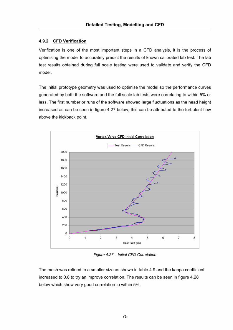
75
Detailed Testing, Modelling and CFD
4.9.2 CFD Verification
Verification is one of the most important steps in a CFD analysis, it is the process of
optimising the model to accurately predict the results of known calibrated lab test. The lab
test results obtained during full scale testing were used to validate and verify the CFD
model.
The initial prototype geometry was used to optimise the model so the performance curves
generated by both the software and the full scale lab tests were correlating to within 5% or
less. The first number or runs of the software showed large fluctuations as the head height
increased as can be seen in figure 4.27 below, this can be attributed to the turbulent flow
above the kickback point.
Vortex Valve CFD Initial Correlation
0
200
400
600
800
1000
1200
1400
1600
1800
2000
0 1 2 3 4 5 6 7 8Flow Rate (l/s)
Hea
d (m
)
Test Results CFD Results
Figure 4.27 – Initial CFD Correlation
The mesh was refined to a smaller size as shown in table 4.9 and the kappa coefficient
increased to 0.8 to try an improve correlation. The results can be seen in figure 4.28
below which show very good correlation to within 5%.

76
Detailed Testing, Modelling and CFD
Manhole Outlet
Walls PipeAngular Resolution (°) 15 30 15 30 15Max. Edge Length (mm) 24 50 24 50 24Min. Edge Length (mm) 8 10 8 10 8
Vortex Chamber
Manhole Opening
Outlet Pipe
Table 4.9 – Modified Mesh Settings
Vortex Valve CFD Final Correlation
0
200
400
600
800
1000
1200
1400
1600
1800
2000
0 1 2 3 4 5 6 7 8Flow Rate (l/s)
Hea
d (m
)
CFD Results Test Results
Figure 4.28 – Final CFD Correlation
CFD is a very useful tool in simulating fluid flow through the vortex valve and can be
accurately used to predict the performance of the flow control device. It does however
have some downsides in that solution time was approximately between 7 – 8 hours for
good correlation. The software is difficult to learn and an in-depth knowledge of fluid
mechanics and CFD is required for selecting the appropriate settings and options during
model set up. However it gives the designer great flexibility to investigate “what if” design
changes to the geometry and once the model is set up the same settings can be used for
various geometries.

77
Chapter 5 Conclusions and Recommendations
5.0 Conclusion
Following a review of all current vortex flow control valves it was found that they all
required a flat face manhole for installation whereas a standard storm water manhole is a
circular shape of 1.2meters internal diameter. Three mounting concepts were developed
to allow for easy installation in a standard 1.2meter storm water manhole, the concepts
evolved from one to the next with concept 3 chosen as the model to develop into a
detailed design. The vortex chamber was redesigned to allow for more efficient material
usage and to optimise the manufacturing process.
A detailed design was developed using mounting concept 3 and the redesigned vortex
chamber to provide the final over all design. The mounting coupler was rotationally
moulded from polyethylene due to its intricate design, the vortex chamber was fabricated
from polyethylene because of its simple geometry. The final design was manufactured
from polyethylene plastic which provided big advantages over the current units on the
market in the areas of cost of materials, cost of manufacture and simplified installation.
A full scale test rig was designed and developed to test the relationship between the
geometric variables of the vortex valve, namely the outlet opening diameter, the width of
the vortex valve, the inlet height and the swirl diameter. An over ground high density
polyethylene manhole was used to install the vortex valve, water was supplied to the
manhole to simulate hydrostatic head from a header tank. The flow through the vortex
valve was measured by keeping the head constant and weighing the volume of water that
passed through the valve over a period of thirty seconds. The weight increment in kg’s
divided by thirty provided the mass flow rate in kg/s and therefore l/s assuming a water
density of 1000kg/m³.
A prototype vortex valve was tested to provide its performance curve of hydrostatic head
in meters versus flow rate in litres per second. The curve followed the general “S” shape
of vortex flow control devices and clearly showed its flush flow point, kickback point and
design flow range. The kickback part of the curve was found to be the extra hydrostatic
head required to initiate the vortex due to the air pocket trapped in the top of the vortex
chamber.
The first geometric variable varied was the outlet opening diameter, this showed a linear
increase in design flow, kickback flow and flush flow as the diameter was increased. It
showed a linear decrease in the head height required to reach the flush flow and kickback

78
Conclusions and Recommendations
flow points due to the smaller air pocket trapped in the vortex chamber as the outlet
opening diameter increased.
Increasing the width of the vortex valve linearly increased the design flow, kickback flow
and flush flow. It showed a non linear increase in the head height required to reach the
flush flow and kickback flow points.
Increasing the inlet height of the vortex valve linearly increased the design flow, kickback
flow and flush flow. It showed a non linear decrease in the head height required to reach
the flush flow and kickback flow points.
The optimum relationship between the geometric variables that satisfies the design
objectives is a ratio of 4:1 between the swirl diameter and the outlet opening diameter
which provided an outlet opening CSA 4 times that of an orifice plate. A ratio of 4:1 was
also used with the width and inlet height as it provided the minimum chance of blockage
with similar sized inlet and outlet openings while maximizing the flow through the vortex
valve to minimise storage requirements.
Varying the swirl diameter while keeping a constant relationship with the other variables
linearly increased the design flow above the kickback point but non linearly increased the
flush flow and kickback flow points. It approximately linearly increased the head height
required to reach the kickback and flush flow points.
A model was built to determine the required geometry of the vortex valve for a given flow
rate and head height specification based on all the testing results. Two models were then
developed to predict the performance curve of a specific geometry vortex valve, the first
model used a unique swirl diameter for each specification with the second model using
the nearest available standard size vortex valve and modifying the outlet opening
diameter to provide the required specification. The first model could accurately predict the
performance curve above the kickback point but not below it, the second model could
accurately predict the entire performance curve by varying the outlet opening diameter of
a standard size unit.
A CFD model was developed to simulate the flow through the vortex valve using Ansys
CFX software, the model set up was complex but once developed it did accurately model
the performance of the vortex valve and was correlated using full scale test results. To
obtain good correlation a solution time of 7 - 8 hours was required on a high performance
computer

79
Conclusions and Recommendations
5.1 Recommendations The following recommendations are outlined for future work in the subject.
• To use computational fluid dynamics to determine the optimum geometric
relationship for flow rates above 20 l/s that will fit in a standard Ø1.2m storm water
manhole.
• To design a conical flow control device for a standard Ø1.2m storm water
manhole.
• To perform the same set of tests on a conical vortex flow control device to identify
geometric relationships and build geometric and performance models.
• Investigate further if computational fluid dynamics can be used to model the fluid
flow through the vortex valve in under one hour to enable designers to quickly
consider the influence of design changes.

80
Chapter 6 References
[1] Office of Public Works, Regional Flooding, OPW Website, viewed 10th of October
2005, <http://www.opw.ie/services/eng_ser/eng_work.htm> [2] P Doyle; B Hennelly; D Mc Entee, “Suds in the Greater Dublin Area” Proceedings
from Pollution Conference, University College Dublin 2003 [3] British Water, Guidance to proprietary sustainable drainage systems and
components, British Water Website, viewed on the 15th November 2005, http://www.britishwater.co.uk/Data/Global/File/Tech%20Guidance%20SUDS.pdf> [4] Woods Ballard B; Kellagher R, The SUDS manual (C697), CIRIA 2007, ISBN 0-86017-697-5 [5] Pijush K. Kundu, Fluid Mechanics, Academic Press, 1990, ISBN 0-12-428780-0 pg 110 [6] W. M. Stallard; W.G. Smith, “Storage Sedimentation Facilities for Control of
Storm and Combined Sewer Overflows” United States Environmental Protection Agency 1997
[7] HydroSlide Website, viewed on the 02nd of December 2005 <http://www.hydrok.co.uk/wms-products-hydroslide.htm> [8] Mosbaek Website, viewed on the 02nd of December 2005 <http://www.mosbaek.dk/index.php?id=34&L=2> [9] Hydro International Website, viewed on the 01st of December 2005 <http://www.hydro-international.biz/stormwater/flowcontrol.php> [10] HydroVex Website, viewed o the 03rd of December 2005 <http://www.hydrovex.com/lib/johnmeunier/3/B2c5jESD8szFH1N6sL5I7.html> [11] Vortechnics Website, viewed on the 05th of December 2005 <http://www.vortechnics.com/stormwater/products/flow_control/hydrobrake/94 [12] Hans J Lugt, Vortex Flow in Nature and Technology, Publisher 1995, ISBN 6-89464-916-7, pages 3,18 and 30 [13] John D. Anderson, JR., “Computational Fluid Dynamics – The Basics with
Applications” McGraw-Hill, 1995, ISBN 0-07-113210-4, Pages 37-38 [14] Ansys Incorporated, “Ansys CFX 10 Users Manual” Ansys Incorporated, 2005 [15] Rodger Toogood, “Pro Engineer Wildfire”, SDC Publications, 2003 [16] CPM Concrete Website, viewed on the 12th of December 2005 <http://www.cpm-group.co.uk/hydrobrake.php> [17] Tracey Concrete Website, viewed on the 12th of December 2005 <http://www.traceyconcrete.com/manholes1.html> [18] J Hannah, M.J. Hiller, “Applied Mechanics” Longman Scientific & Technical 1988, ISBN 0-583-98820-9, page 463 and 464
81
References
[19] Weakly swirling turbulent flow in turbid water hydraulic separation device
Journal of Hydrodynamics, Ser. B, Volume 20, Issue 3, June 2008, Pages 347-355 Lin LI, Xiu-yun QIU, Sheng JIN, Jun XIAO, Shou-yuan GONG
[20] A CFD methodology for the design of sedimentation tanks in potable water
treatment: Case study: The influence of a feed flow control baffle Chemical Engineering Journal, Volume 140, Issues 1-3, 1 July 2008, Page 110 Athanasia M. Goula, Margaritis Kostoglou, Thodoris D. Karapantsios, Anastasios I. Zouboulis
[21] Multiple vortex formation in steady laminar axisymmetric impinging flow
Computers & Fluids, Volume 37, Issue 9, October 2008, Pages 1061-1076 Ajay Chatterjee