design and development of an acoustic positioning - riunet - upv
TRANSCRIPT
Julio 2012
ESCUELA POLITECNICA SUPERIOR DE GANDIA
Departamento de Física Aplicada
Giuseppina Larosa
Design and Development of an acoustic
positioning system for a cubic kilometre
underwater neutrino telescope
Tesis Doctoral
Director de tesis:
Dr. Miguel Ardid Ramírez


“Alla mia famiglia
&
a Demetrio”

CONTENTS.
I
Contents
Summary of doctoral thesis (in English, Spanish and
Catalan) 1
Introduction 13
1 Principles and Applications to Underwater Acoustics 15
1.1 History of the applications to underwater acoustics…………….....15
1.2 Underwater Electro-Acoustic Transducers………………………...17
1.2.1 Underwater acoustic sources and hydrophones……………….....20
1.2.1.1 Tonpilz transducers………………………………………...20
1.2.1.2 High-frequency transducer………………………………....21
1.2.1.3 Low-frequency transducer………………………………....22
1.2.1.4 Hydrophones…………………………………………….....24
1.3 Underwater Acoustics Applications…………………………….....25
1.3.1 Military applications……………………………………………..26
1.3.2 Civilian applications…………………………………………......27
1.4 Acoustic Positioning…………………………………………….....28
2 Acoustic Positioning System in Underwater Neutrino
Telescopes 31
2.1 Underwater Neutrino Telescopes……………………………….....31
2.2 Acoustic Positioning System of the ANTARES detectors ……....34
2.3 NEMO Acoustic Positioning System ………………………….....38
2.4 KM3NeT detector and the proposed Acoustic Positioning
System…………………………………………………………......44
3 Transceiver for the KM3NeT Acoustic Positioning
System 51
3.1 Transceiver for the KM3NeT Acoustic Positioning System….......51

CONTENTS.
II
3.1.1 The Acoustic Sensors…………………………………………...51
3.1.2 The Sound Emission Board……………………………………..54
3.1.2.1 Microcontroller and Signal generator block……………...56
3.1.2.2 The firmware……………………………………………...57
3.2 Sensitivity tests of the FFR-SX30………………………………...58
3.3 Pressure tests……………………………………………………....65
3.4 Tests on the Transceiver…………………………………………..70
3.4.1 Sensitivity tests of the system…………………………………...71
3.4.2 Functionality tests of the system………………………………...73
4 Integration of the acoustic transceiver in Underwater
Neutrino Telescopes 81
4.1 Integration in ANTARES Neutrino Telescope................................81
4.1.1 SEB for the integration in ANTARES detector………………....85
4.1.2 Transmitting Power of the system for the ANTARES
detector………………………………………………………......88
4.2 Integration in NEMO detector…………………………………......92
4.2.1 Transmitting Power of the system for NEMO detector…….........94
4.2.2 NEMO Phase II joint acoustic tests ………………………..........98
Conclusions 105
Acronyms 109
References 113
Acknowledgments 119
SUMMARY.
1
Summary Context
Lately underwater neutrino telescopes have become very important since it is a new and
unique method to observe the Universe. The neutrinos are uncharged particles and
interact weakly with matter. They can escape from sources which have produced them
and arrive to the Earth unperturbed by magnetic fields and without interaction with
other particles. This means that neutrinos can bring us astrophysical information that
other messengers cannot and, then they can open a potential new window on the
Universe.
On the other hand, their low interaction cross section imposes to build very large
detectors with dimensions of ~1 km3. Therefore, it is necessary the instrumentation of
large volumes of water (or ice) with several optical sensors in order to detect
characteristic signatures of high energy neutrino interactions. One way to detect
neutrino interactions can be afforded through the detection of the Cherenkov light
emitted by the muon generated after a neutrino interaction. This particle travels across
the detector at a speed greater than the speed of light in water, so generating a faint blue
luminescence called Cherenkov radiation, which can be detected through an array of
optical sensors (photomultipliers). The arrival times of the light collected by
photomultipliers can be used to reconstruct the muon track, and consequently that of the
neutrino, which has produced it. The accuracy of the reconstruction of the muon track
depends on the precision in the measurement of the light arrival time and on precise
knowledge of the positions of the optical detectors. For this reason, in an underwater
telescope an acoustic positioning system (APS) able to monitoring the position of the
optical sensors with an accuracy of ~10 cm is necessary (about the length of the
photomultipliers diameter). The studies in this thesis have been developed within the
framework of acoustic position calibration in two European collaborations for the
design, building and operation of an underwater neutrino telescope in the Mediterranean
Sea: ANTARES (in operation phase) and KM3NeT (in preparatory phase for the
construction).
Summary

SUMMARY.
2
In this thesis the work and the results for designing, developing, testing and
characterizing a prototype of acoustic transceiver to be used in the APS of the future
KM3NeT neutrino telescope are presented.
Objectives
The goals of this thesis can be summarized in the following aspects:
- Design of the acoustic transceiver for the APS of KM3NeT.
- Development of the acoustic transceiver prototype.
- Characterization of the transceiver in the laboratory and in the sea.
- Adapting the prototype for its integration in ANTARES and NEMO sites for the
in situ test.
Elements of the methodology to emphasize
We would like to remark that the work of the thesis has been developed within the
international consortium KM3NeT, funded with European and National funds.
Due to the context and the nature of the activities done it has been necessary training in
different fields: neutrino telescopes and astroparticles, but also in other field such as
underwater acoustics or transducers. Moreover, different skills and abilities in different
application fields have been developed: instrumentation, design and characterization of
the acoustic system in water, data analysis, etc. Particularly, in order to design the
transceiver, the acoustic transducer has been chosen according to the performance for
the proposed application and afterwards specific electronics has been designed.
Different configurations of the measurements have been set up to test and prove the
prototype, the different measurements have been analyzed and the results and
conclusions have been obtained. Finally, the tasks towards the integration in underwater
neutrino telescopes have been done.
Results
Different studies for the development and testing of a prototype of transceiver for the
proposed APS of KM3NeT have been done. The prototype consists of a transducer type
Free Flooded Ring FFRSX30 with 20-40 kHz frequency range and an electronic board
named SEB (Sound Emission Board), especially designed for it. The SEB is able to
manage the emission and reception of different signals, as well as allowing the
communication and configuration of the system. In a first step, the characterization of
SUMMARY.
3
the hydrophones has been done in order to study the sensitivity and its dependence at
high pressure (up to 440 bars). In a second step, the whole system (FFRSX30 plus SEB)
has been tested and characterized in different conditions (tank, water pool and harbour
of Gandia) in order to integrate it in the ANTARES, NEMO and KM3NeT neutrino
detectors. The proposed transducers have good characteristics for their application for
the KM3NeT APS and they can also be used as receivers, but in this case a good
parameterisation of the sensitivity as a function of the frequency and angle for each
transducer will be needed.
The transducers have a very low intrinsic noise ~ -120 dB re V2/Hz (~ ≤Sea State 1) and
they are quite stable at different pressures, that is with depth. For simplicity and due to
limitations to the integration in both detectors, it was decided to test the transceiver only
as emitter. The receiver functionality will be tested successively in other tests. The
changes performed in the transceiver in order to integrate it in the different detectors
show that the system is versatile and adaptable to the different conditions. The system,
with low power consumption, is able to have a transmitting power above 170 dB re
1µPa@1m that combined with signal processing techniques allow to deal with the large
distances involved in a neutrino telescope.
In conclusion, the system has been integrated with success in ANTARES and NEMO
neutrinos telescopes and, after being proved in situ, it will be implemented in the final
configuration of the KM3NeT detector. Finally, we would like to remark that the
acoustic system proposed is compatible with the different options for the receiver
hydrophones proposed for KM3NeT and it is versatile, so in addition to the positioning
functionality, it can be used for neutrino acoustic detection studies or for acoustic
monitoring studies in deep-sea. Moreover, the transceiver (with slight modifications)
may be used in other acoustic positioning systems or emitter-receiver systems, alone or
combined with other marine systems, where the localization of the sensors is an issue.
In that sense, the experience gained from this research can be of great use for other
possible applications.
Acknowledgments
This work has been supported by the Ministerio de Ciencia e Innovación (Spanish
Government), project references FPA2009-13983-C02-02, ACI2009-1067; and the
European 6th and 7th Framework Programme, contract no. DS 011937 and grant no.
212525, respectively.

4

SUMMARY.
5
Resumen Contexto.
En los últimos años los telescopios submarinos de neutrinos han cobrado una mayor
importancia ya que consisten en un nuevo y único instrumento para observar el
Universo. Los neutrinos son partículas sin carga e interactúan muy débilmente con la
materia que les rodean, pueden escaparse fácilmente de la fuente que los ha producidos
y llegar a La Tierra sin ser desviada por los campo magnético y sin interactuar con otras
partículas. Esto implica que los neutrinos pueden traer informaciones astrofísicas que
otros mensajeros no pueden aportar y abrir una potencial ventana hacia el Universo.
Por otro lado, su baja interacción con la materia impone la necesidad de construir un
detector de grandes dimensiones del orden de 1 km3 utilizando volumen de agua o hielo
y con muchos sensores ópticos para detectar esta interacción de neutrino de alta energía.
Un método para detectar neutrinos es a través de la luz Cherenkov emitida por el muon
generado después de una interacción de neutrino. Esta partícula, al atravesar el detector
con una velocidad superior a la luz en el medio, genera una débil luz azulada llamada
radiación de Cherenkov que es detectada por una red de sensores ópticos
(fotomultiplicadores). El tiempo de llegada de la luz a los fotomultiplicadores puede ser
utilizado para reconstruir la traza del muon y consecuentemente del neutrino que lo ha
producido. La precisión en la reconstrucción de la traza del muon depende de la
precisión en la medida del tiempo de llegada de la luz y en la precisión en de la posición
de los sensores ópticos en el detector. Por esta razón, en telescopios submarinos es
necesario un sistema de posicionamiento acústico (APS) capaz de monitorizar el
movimiento de los sensores ópticos con una precisión de ~10 cm (prácticamente la
longitud del diámetro del fotomultiplicador). Los estudios realizados están enmarcados
dentro de las actividades de calibración de posicionamiento acústico en dos
colaboraciones europeas para el diseño, construcción y operación de telescopios
submarinos de neutrinos en el Mediterráneo: ANTARES (en fase de operación) y
KM3NeT (en fase de preparación para la construcción).
Síntesis.
En esta tesis se presentan los trabajos y resultados para el diseño, desarrollo, test y
caracterización de un prototipo de transceptor acústico para ser utilizado en el APS del
futuro telescopio de neutrinos KM3NeT.
SUMMARY.
6
Objetivos.
Los objetivos de este trabajo pueden resumirse en los siguientes aspectos:
- Diseño del transceptor acústico para el APS de KM3NeT.
- Desarrollo del prototipo de transceptor acústico.
- Caracterización del transceptor en el laboratorio y en el mar.
- Adaptación del prototipo para su integración en ANTARES y NEMO sites para
su validación in situ.
Elementos de la metodología a destacar.
Cabe destacar aquí que el trabajo se ha desarrollado en el marco del consorcio
internacional KM3NeT, financiado con fondos europeos y nacionales. Por su contexto y
el carácter de las actividades realizadas ha sido necesaria la formación en distintos
campos: telescopios de neutrinos y astropartículas, pero también en otras áreas como la
acústica submarina y los transductores. Además, se ha desarrollado diversas
capacidades y destrezas en diversos ámbitos: en instrumentación, en diseño y
caracterización de sistemas acústicos en agua, en análisis de datos, etc.
Más concretamente, para el diseño del transceptor se ha elegido el transductor acústico
con mejores prestaciones para la aplicación propuesta y se ha diseñado la electrónica.
También se ha realizado diferentes configuraciones de medidas para testear y validar el
prototipo, se han analizado las diferentes medidas y se ha obtenido los resultados y
conclusiones. Finalmente, se ha realizado las labores para su integración en telescopios
de neutrinos submarinos.
Resultados logrados.
Se ha realizado el estudio, desarrollo y test de un prototipo de transceptor para el APS
de KM3NeT propuesto. El prototipo es constituido por un transductor de tipo Free
Flooded Ring FFRSX30 con rango de trabajo desde 20 kHz hasta 40 kHz y una tarjeta
electrónica llamada SEB (Sound Emission Board) capaz de controlar la emisión y
recepción de diferentes señales. En primer lugar, se ha caracterizado los transductores
con el fin de estudiar su sensibilidad y su dependencia a elevada presión (hasta 440 bar).
En segundo lugar se ha testeado y caracterizado el sistema entero (FFRSX30 más SEB)
en diferentes condiciones ambientales (tanque, piscina y puerto de Gandia) con el
SUMMARY.
7
objetivo de integrarlo en los detectores de neutrinos ANTARES, NEMO y KM3NeT.
Cabe destacar que los transductores propuestos presentan buenas características para su
aplicación en el APS del detector KM3NeT e incluso se podrían utilizar como
receptores, aunque se tendrían que considerar sus dependencias en sensibilidad para
diferentes frecuencias y ángulos. Tienen un ruido intrínseco muy bajo ~ -120 dB re
V2/Hz (~ ≤ Sea State 1) y son bastantes estables al variar de la presión, es decir, con la
profundidad. Por simplicidad y debido a las limitaciones por su integración en los
detectores, se ha decidido de utilizar el sistema solo como emisor y la funcionalidad
como receptor será testeada sucesivamente en otras configuraciones. Los cambios
aportados por la integración en los diferentes detectores destacan que el sistema es muy
versátil y capaz de adaptarse a las diferentes condiciones. El sistema tiene baja potencia
de consumo y es capaz de obtener una potencia de trasmisión mayor que 170 dB re
1µPa @ 1 m que combinado con técnicas de procesado de señal permitiría llegar a las
largas distancias implicadas en los telescopios de neutrinos.
En conclusión, el sistema se ha integrado positivamente en los telescopios de neutrinos
ANTARES y NEMO y, tras su validación in situ, será implementado en la
configuración final del detector KM3NeT. Además, se remarca que el sistema propuesto
es compatible con las diferentes opciones para hidrófonos propuestos para KM3NeT y
es versátil, con lo que puede ser utilizado también en el estudio de la detección de
neutrinos o estudios de monitorización acústica en el mar. Asimismo, el sistema (con
algunas modificaciones) puede ser utilizado en otros sistemas de posicionamiento
acústico o sistemas de emisión-recepción, autónomos o combinado con otros sistemas
marinos, y en donde la localización de los sensores es clave. En este sentido, la
experiencia ganada a través de esta investigación puede ser de gran valía para otras
posibles aplicaciones.
Agradecimientos.
Este trabajo ha sido financiado por el Ministerio de Ciencia e Innovación (Gobierno de
España), proyectos referencia FPA2009-13983-C02-02, ACI2009-1067; y el 6º y 7º
Programa Marco Europeo, Contract no. DS 011937 y Grant no. 212525,
respectivamente.

8
SUMMARY.
9
Resum Context.
En els últims anys els telescopis submarins de neutrins han cobrat una major
importància ja que consisteixen en un nou i únic instrument per observar l'Univers. Els
neutrins són partícules sense càrrega i interactuen molt dèbilment amb la matèria que els
envolten, poden escapar fàcilment de la font que els ha produït i arribar a La Terra sense
ser desviats pels camps magnètics i sense interactuar amb altres partícules. Això implica
que els neutrins poden portar informacions astrofísiques que altres missatgers no poden
aportar i obrir una potencial nova finestra cap a l’Univers. D'altra banda, la seva baixa
interacció amb la matèria imposa la necessitat de construir un detector de grans
dimensions, de l'ordre d'1 km3, mitjançant un gran volum d'aigua o gel i amb molts
sensors òptics per detectar aquesta interacció de neutrí d'alta energia. Un mètode per
detectar neutrins és a través de la llum Cherenkov emesa pel muó generat després d'una
interacció de neutrí. Aquesta partícula, en travessar el detector amb una velocitat
superior a la llum en el medi, genera una feble llum blavosa anomenada radiació de
Cherenkov que és detectada per una xarxa de sensors òptics (fotomultiplicadors). El
temps d'arribada de la llum als fotomultiplicadors pot ser utilitzat per reconstruir la traça
del muó i conseqüentment del neutrí que l'ha produït. La precisió en la reconstrucció de
la traça del muó depèn de la precisió en la mesura del temps d'arribada de la llum i en la
precisió de la posició dels sensors òptics en el detector. Per això, en telescopis
submarins és necessari un Sistema de Posicionament Acústic (APS) capaç de
monitoritzar el moviment dels sensors òptics amb una precisió de ~ 10 cm
(pràcticament el diàmetre del fotomultiplicador). Els estudis realitzats estan emmarcats
dins de les activitats de calibratge de posicionament acústic en dues col·laboracions
europees per al disseny, construcció i operació de telescopis submarins de neutrins a la
Mediterrània: ANTARES (en fase d'operació) i KM3NeT (en fase de preparació per a la
construcció).
Síntesi.
En aquesta tesi es presenten els treballs i resultats per al disseny, desenvolupament, test
i caracterització d'un prototip de transceptor acústic per ser utilitzat en l'APS del futur
telescopi de neutrins KM3NeT.
SUMMARY.
10
Objectius.
Els objectius d'aquest treball es poden resumir en els següents punts:
- Disseny del transceptor acústic per a l’APS de KM3NeT.
- Desenvolupament del prototip de transceptor acústic.
- Caracterització del transceptor al laboratori i al mar.
- Adaptació del prototip per a la seva integració en ANTARES i NEMO sites per a la
seva validació in situ.
Elements de la metodologia a destacar.
Cal destacar aquí que el treball s'ha desenvolupat en el marc del consorci internacional
KM3NeT, finançat amb fons europeus i nacionals. Pel context i el caràcter de les
activitats realitzades ha estat necessària la formació en diferents camps: telescopis de
neutrins i astropartícules, però també en altres àrees com l'acústica submarina i els
transductors. A més, s'ha desenvolupat diverses capacitats i destreses en diversos
àmbits: en instrumentació, en disseny i caracterització de sistemes acústics en aigua, en
anàlisi de dades, etc.
Més concretament, per al disseny del transceptor s'ha triat el transductor acústic amb
millors prestacions per a l'aplicació proposta i s'ha dissenyat l'electrònica. També s’han
realitzat diferents configuracions de mesures per testejar i validar el prototip, s'han
analitzat les diferents mesures i s'han obtingut els resultats i conclusions. Finalment,
s'han realitzat les tasques per a la seva integració en telescopis de neutrins submarins.
Resultats assolits.
S'ha realitzat l'estudi, desenvolupament i test d'un prototip de transceptor per a l’APS de
KM3NeT proposat. El prototip és constituït per un transductor de tipus Free Flooded
Ring FFRSX30 amb rang de treball des de 20 kHz fins a 40 kHz i una targeta
electrònica anomenada SEB (Sound Emission Board) capaç de controlar l'emissió i
recepció de diferents senyals. En primer lloc, s'ha caracteritzat els transductors amb la
finalitat d'estudiar la seva sensibilitat i la seva dependència a elevada pressió (fins a 440
bar). En segon lloc s'ha testejat i caracteritzat el sistema sencer (FFRSX30 més SEB) i
s’ha provat el sistema en diferents condicions ambientals (tanc, piscina i port de Gandia)
amb l'objectiu d'integrar-lo en els detectors de neutrins ANTARES, NEMO i KM3NeT.
Cal destacar que els transductors proposats presenten bones característiques per a la
SUMMARY.
11
seva aplicació en l'APS del detector KM3NeT i fins i tot es podrien utilitzar com a
receptors, encara que s'haurien de considerar les seves dependències en sensibilitat per a
diferents freqüències i angle. Tenen un soroll intrínsec molt baix ~ -120 dB re V2/Hz (~
≤ Sea State 1) i són bastant estables en variar la pressió, és a dir, amb la profunditat. Per
simplicitat i a causa de les limitacions per la seva integració en els detectors, s'ha decidit
d'utilitzar el sistema només com a emissor i la funcionalitat com a receptor serà testada
successivament en altres configuracions. Els canvis aportats per a la integració en els
diferents detectors destaquen que el sistema és molt versàtil i capaç d'adaptar-se a les
diferents condicions. El sistema té baixa potència de consum i és capaç d'obtenir una
potència de transmissió major que 170 dB re 1µPa @ 1 m que combinat amb tècniques
de processament del senyal permetria arribar a les llargues distàncies implicades en els
telescopis de neutrins.
En conclusió, el sistema s'ha integrat positivament en els telescopis de neutrins
ANTARES i NEMO i, després de la seva validació in situ, serà implementat a
configuració final del detector KM3NeT. A més, es remarca que el sistema proposat és
compatible amb les diferents opcions d’hidròfons proposats per KM3NeT, i és versàtil,
amb la qual cosa podria ser utilitzat també en l'estudi de la detecció de neutrins o estudis
de monitorització acústica al mar. Així mateix, el sistema (amb algunes modificacions)
podría ser utilitzat en altres sistemes de posicionament acústic o sistemes d'emissió-
recepció, autònoms o combinats amb altres sistemes marins, on la localització dels
sensors és clau. En aquest sentit, l'experiència guanyada a través d'aquesta investigació
pot ser de gran interés per a altres possibles aplicacions.
Agraïments.
Aquest treball ha estat finançat pel Ministeri de Ciència i Innovació (Govern espanyol),
projectes referència FPA2009-13.983-C02-02, ACI2009-1067; i el sisé i seté Programa
Marc Europeu, Contract no. DS 011937 i Grant no. 212525, respectivament.

12
INTRODUCTION.
13
Introduction
The seas and oceans comprise more than 70% of the Earth’s surface, and as a natural
resource of raw materials, fuel and food, they have never been as important as today.
The deep sea is mostly dark, optically opaque and does not allow for propagation of
electromagnetic waves since salt water exhibits a strong conductivity, and is therefore
highly dissipative. Contrarily, the water is acoustically transparent and is a natural
medium for the effective transmission of acoustic waves, carrying information
underwater. In this thesis underwater acoustics is applied for the position calibration
systems of deep-sea neutrino telescopes. Recently, neutrino telescopes have become an
important tool of astroparticle physics, providing a new and unique method to observe
the Universe. Neutrinos are uncharged particles and interact weakly with matter. They
can escape from the sources which have produced them and arrive at the Earth
unperturbed by magnetic fields and without interaction with other particles. This means
that neutrinos can bring us astrophysical information that other particles cannot and,
opening a potential new window to the Universe. The studies done in this thesis have
been developed within the framework of the design and prototyping for the acoustic
position calibration of the future KM3NeT deep-sea neutrino telescope. The outline of
the thesis is as follows.
In Chapter 1 the history of applications of underwater acoustics will be overviewed as
well as the use of underwater transducers, either as acoustic sources or as underwater
acoustic receivers. Moreover a brief sketch on the military and civilian application will
be described. Particularly, the application of the acoustic positioning, nucleus of this
thesis, will be deeply described.
Since the main aim of this work is the acoustic positioning system in underwater
neutrino telescopes, Chapter 2 focuses on the description of underwater neutrino
telescopes and of the different detector developed that are in operation and in
construction. In particular, we will pay attention to their acoustic positioning systems in
order to describe the basis for the new acoustic positioning system proposed for the new
and bigger KM3NeT underwater detector.
Chapter 3 presents the experiments and tests which have been carried out to design,
develop and characterise the acoustic transceiver for the KM3NeT positioning system.

INTRODUCTION.
14
The transducers and electronics used and the tests done on them are described in detail,
as well as the tests of the whole system in different environments (tank, pool and
harbour) in order to prove the system in different conditions. The results of these tests
are also discussed.
Finally, the activities for the integration of the acoustic transceiver prototype in the
ANTARES and NEMO neutrino detectors are detailed in Chapter 4. The expected
behavior of the transducer as well as the expected pressure and signals obtained by the
ANTARES/AMADEUS and NEMO hydrophones are presented. A data analysis of the
latest tests realized with this prototype and the results are also described and discussed.
CHAPTER 1. Principles and Applications to Underwater Acoustics
15
Chapter 1
Principles and Applications to Underwater Acoustics
1.1 History of the applications to underwater acoustics
The oceans are a vast, complex, mostly dark, optically opaque but acoustically
transparent world that has been only thinly sampled by today’s limited technology and
means of science. Underwater acousticians and acoustical oceanographers use sound as
the premier tool to determine the detailed characteristics of physical and biological
bodies and processes at sea. Myriad components of the ocean world are being
discovered, identified, characterized, and imaged by their interactions with sound
[MED05]. In fact, the possibility of using sound to detect distant ships, by simply
listening to the noise they radiate into the water, has apparently been known for a very
long time. Leonardo da Vinci is often mentioned as the first to propose this. But
practical applications have been more recent, and the first underwater acoustic devices
used efficiently were the passive detection systems developed by the Allies during
World War I, to counter the then new threat of German submarines. The idea that
obstacles to navigation and targets in warfare could be detected by active acoustic
systems has been studied from the beginning of the 20th century, in particular, after the
steamship Titanic struck an iceberg in 1912. Within a month of the disaster, a patent
application was filed by L.R. Richardson in the United Kingdom (10 May 1912) for
“detecting the presence of large objects under water by means of the echo of
compressional waves (directed in a beam) by a projector”. The basic idea was that a
precise knowledge of the speed of sound in water, and the travel time of the sound from
source to scattered and back to the source/receiver, permits the calculation of the
distance to the scattering body. This was to be the beginning of the use of underwater
sound projectors and receivers. They were to be called “SONARs” i.e., devices for
Sound Navigation and Ranging [MED05]. But, a major breakthrough came from Paul
Langevin, a French physicist, where during groundbreaking experiments on the River
Seine and at sea, between 1915 and 1918, he demonstrated that it was possible to
transmit signals, and to actively detect submarines, giving both their angles and
CHAPTER 1. Principles and Applications to Underwater Acoustics
16
distances from the receiver. His decisive innovation consisted in using a piezoelectric
transducer to replace capacitive transducer. With Langevin’s invention more efficient
sandwich transducer bore. Although these developments came too late to be of much
use against submarines in World War I, numerous technical improvements and
commercial applications followed rapidly [DAV02].
Between the two world wars, sonar technology improved considerably. It benefited
from the emergence of first-generation electronics and from progress in the newborn
radio industry. At the beginning of World War II, the technology of active sonar was
advanced enough to be used on a large scale by the Allied navies (these were the famed
ASDIC systems of the Royal Navy). In particular, the USA entered the war in 1941 and
made a huge effort in sonar research and development. This greatly improved the
performance of active sonar systems, as well as the understanding of underwater
acoustic propagation, or the theories associated with detection and measurement of
signals buried in noise.
After the war had ended in 1945, the “Cold War” between the Western and Eastern
blocks resulted in continued efforts in scientific and technological research would
continue. In the following years, in the West and in the Soviet Union, large programmes
of research and experimentation were started. At the end of the 1950s, a new impulse
was given by the appearance of nuclear submarines capable of launching strategic
missiles, followed swiftly by the production of attack nuclear submarines. This led to a
complete review of underwater warfare strategies since until then, the sonar was used
locally to monitor ship convoys or shipping corridors. Now, it had to be able to monitor
vast areas of the oceans. In the 1960s, priority was thus given to the study of passive
detection techniques, capable of achieving much larger ranges than active acoustics. A
technological revolution occurred at the end of the 1960s, with the introduction of
digital signal processing. This led to the increase in capabilities and versatility of sonar
systems. The extreme degree of sophistication reached at this time by passive sonar
was, however, countered by progress in reducing acoustic noise radiated by submarines.
So the trend was again reversed in the 1990s, with a return of active sonar techniques,
extended to lower frequencies (to reach larger ranges). Those studies at the end of the
20th century confirmed the importance of mastering sonar techniques to counter the
treats of attack submarines or of mines.
In parallel with military developments, oceanography and industry were able to profit
from the development of underwater acoustics. Acoustic sounders quickly replaced the
CHAPTER 1. Principles and Applications to Underwater Acoustics
17
traditional lead line to measure the water depth below a ship or to detect obstacles. It
became widely used between the two world wars and today these systems are both
scientific instruments and indispensable navigation tools. These same systems began to
be used to detect fish shoals early in the 1920s; underwater acoustics has progressively
become one of the main elements of sea fishing and scientific monitoring of the
biomass. The use of sidescan sonars to obtain “acoustic images” from the seabed
became one of the major tools of marine geology after their invention in the early
1960s. The efficiency of seabed acoustic mapping increased dramatically with the
emergence in the 1970s of multibeam echosounders, allowing multiplication of the
number of simultaneous soundings. Merged with sidescan imagery at the end of the
1980s, this concept today allows for the collection of maps of remarkable quality, which
measure both the topography of the seabed and its acoustic reflectivity (i.e., yielding
insights into its nature). The offshore oil and underwater industries were also concerned
with acoustic mapping developments. They initiated the development of specific
acoustic techniques for the positioning of ships or underwater vehicles, or for data
transmission. In the domain of physical oceanography, the propagation of acoustic
waves has been used since the 1970s to measure hydrological perturbations locally
(acoustic Doppler current profiling) or on a medium scale (ocean acoustic
tomography). Techniques of acoustic monitoring have even been suggested to monitor
the evolution of the average temperature of large ocean basins on a permanent basis, as
part of global climate studies.
Therefore, the number and type of applications has grown and underwater acoustics
today plays in the ocean the same essential role played by radar and radio waves in the
atmosphere and in space [LUR 02].
1.2 Underwater Electro-Acoustic Transducers
During the years, underwater electro-acoustic transducers have been instrumental for
the transmission and reception of underwater acoustic signals. They convert acoustic
energy into electric energy and vice versa. Underwater acoustic sources are called
projectors. The reception transducers are called hydrophones. Extended transducers are
named antennas, or arrays. The latter expression is usually reserved for structures made
up of several elementary transducers. A transmitter is made up of a projector and its

CHAPTER 1. Principles and Applications to Underwater Acoustics
18
associated electronics. Similarly, a receiver is made up of a hydrophone array and its
associated low-level electronics (preamplifier and filters).
Underwater acoustic transducers use several physical processes to generate or receive
sound waves. Presumably, 90%-95% of underwater acoustic transducers use the
piezoelectric properties of some crystals, natural or artificial (ceramics). An electric
field applied to these materials causes a deformation related to electrical excitation.
These mechanical deformations in turn create acoustic waves (Fig.1.1). The opposite
effects are used in reception: a piezoelectric material stressed by sound waves will
generate an electric potential between its sides.
Figure 1.1: Piezoelectric effect: (left) transmission: applying an electric signal to a piece of
piezoelectric material induces a mechanical deformation, generating an acoustic wave; (right)
reception: the mechanical stress caused by the acoustic wave is transformed by the piezoelectric
material into an electric voltage [LUR02].
Natural piezoelectric crystals, such as quartz or Seignette salt, were used in the early
days of underwater acoustics. Such crystals are now replaced by synthetic ceramics.
They are produced by mixing components under high temperature and high pressure
(sintering). The resulting material is then machined to the dimensions required and
coated with metal. The ceramics produced is not spontaneously polarized; this is created
artificially by applying a very intense electric field to induce a remnant polarisation.
The piezoelectric effect will be linear and reversible around this remnant polarisation.
The fundamental equations of piezoelectricity link together the mechanical, electrical
and piezoelectrical values of ceramics. As a simple case, we mention here that the
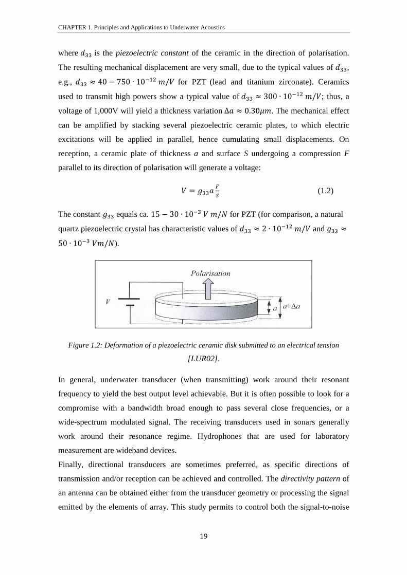
thickness a of a ceramic plate, submitted to a voltage V between its sides (assumed
perpendicular to the direction of polarisation, see Fig. 1.2), will vary proportionally to
the amplitude of the excitation:
∆ = (1.1)
Acoustic waves Piezoelectrico ceramics
Mechanical stress
CHAPTER 1. Principles and Applications to Underwater Acoustics
19
where is the piezoelectric constant of the ceramic in the direction of polarisation.
The resulting mechanical displacement are very small, due to the typical values of ,
e.g., ≈ 40 − 750 ∙ 10/ for PZT (lead and titanium zirconate). Ceramics
used to transmit high powers show a typical value of ≈ 300 ∙ 10/; thus, a
voltage of 1,000V will yield a thickness variation∆ ≈ 0.30. The mechanical effect
can be amplified by stacking several piezoelectric ceramic plates, to which electric
excitations will be applied in parallel, hence cumulating small displacements. On
reception, a ceramic plate of thickness a and surface S undergoing a compression F
parallel to its direction of polarisation will generate a voltage:
=
(1.2)
The constant equals ca. 15 − 30 ∙ 10/ for PZT (for comparison, a natural
quartz piezoelectric crystal has characteristic values of ≈ 2 ∙ 10/ and ≈
50 ∙ 10 /).
Figure 1.2: Deformation of a piezoelectric ceramic disk submitted to an electrical tension
[LUR02].
In general, underwater transducer (when transmitting) work around their resonant
frequency to yield the best output level achievable. But it is often possible to look for a
compromise with a bandwidth broad enough to pass several close frequencies, or a
wide-spectrum modulated signal. The receiving transducers used in sonars generally
work around their resonance regime. Hydrophones that are used for laboratory
measurement are wideband devices.
Finally, directional transducers are sometimes preferred, as specific directions of
transmission and/or reception can be achieved and controlled. The directivity pattern of
an antenna can be obtained either from the transducer geometry or processing the signal
emitted by the elements of array. This study permits to control both the signal-to-noise

CHAPTER 1. Principles and Applications to Underwater Acoustics
20
ratio of the measurement (via the directivity index) and the target angle estimation,
essential in many sonar systems [LUR02].
1.2.1 Underwater acoustic sources and hydrophones
1.2.1.1 Tonpilz transducers
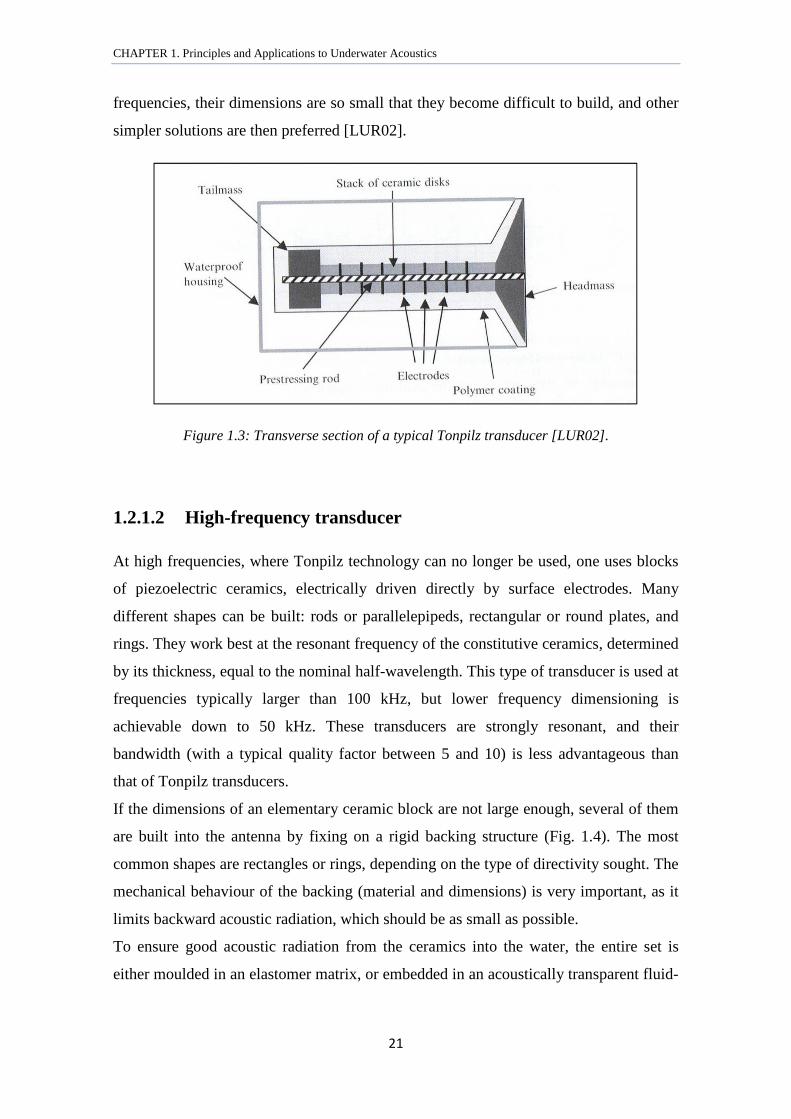
Tonpilz technology is the most frequently used in underwater acoustic transducers.
Piezoelectric ceramic plates are separated by electrodes (Fig. 1.3) and stacked under
strong static pressure imposed by a prestressing rod. This stack is interdependent by the
radiating headmass (balanced by a tailmass at the other end). It transmits to the
surrounding water the vibrations induced by a driving electric field applied along the
electrodes of the stack of piezoelectric disks. The entire system, covered with a polymer
coating, is packaged inside a waterproof housing, filled with air to limit backward
radiation of the headmass. This air filling precludes the use of Tonpilz transducers at
large depths, since the housing risks being crushed by high hydrostatic pressures. Filling
it with oil increases the depth achievable, at the expense or lower sensitivity.
The size of the piezoelectric ceramics that are in the transducer determines the
resonance frequency, the transmission level and the electrical impedance. The diameter
and the thickness of the headmass, acting as a transformer adapting the active ceramics
to the propagation medium, influence both the resonance frequency and the
transmission level. The use of a sufficiently light metal (e.g., aluminum or magnesium)
makes it possible to broaden the bandwidth. The role or the tailmass is to limit
backward acoustic radiation, and to tune the resonance frequency. To be effective, it
must be made of a dense enough material (e.g., steel or bronze).
Tonpilz transducers are based on a resonance concept. They can achieve high
transmission levels with good power efficiency, but they only allow for limited band-
widths. Quality factors as low as 2 or 3 can be obtained (this means that that bandwidth
is
or
of the resonant frequency). Because of their simple design, Tonpilz transducers
are very successful in the majority of applications at frequencies typically between 2
kHz and 50 kHz. At frequency around 1 kHz and below, their size and their weight
make them too cumbersome for practical applications. Conversely, at higher
CHAPTER 1. Principles and Applications to Underwater Acoustics
21
frequencies, their dimensions are so small that they become difficult to build, and other
simpler solutions are then preferred [LUR02].
Figure 1.3: Transverse section of a typical Tonpilz transducer [LUR02].
1.2.1.2 High-frequency transducer
At high frequencies, where Tonpilz technology can no longer be used, one uses blocks
of piezoelectric ceramics, electrically driven directly by surface electrodes. Many
different shapes can be built: rods or parallelepipeds, rectangular or round plates, and
rings. They work best at the resonant frequency of the constitutive ceramics, determined
by its thickness, equal to the nominal half-wavelength. This type of transducer is used at
frequencies typically larger than 100 kHz, but lower frequency dimensioning is
achievable down to 50 kHz. These transducers are strongly resonant, and their
bandwidth (with a typical quality factor between 5 and 10) is less advantageous than
that of Tonpilz transducers.
If the dimensions of an elementary ceramic block are not large enough, several of them
are built into the antenna by fixing on a rigid backing structure (Fig. 1.4). The most
common shapes are rectangles or rings, depending on the type of directivity sought. The
mechanical behaviour of the backing (material and dimensions) is very important, as it
limits backward acoustic radiation, which should be as small as possible.
To ensure good acoustic radiation from the ceramics into the water, the entire set is
either moulded in an elastomer matrix, or embedded in an acoustically transparent fluid-

CHAPTER 1. Principles and Applications to Underwater Acoustics
22
filled housing (most commonly castor oil). This type of equipressure packaging makes
these transducers particularly well suited to large depths.
At high frequencies, another possibility is the composite ceramic technology.
Piezoelectric sticks are grouped to form a given projector shape, and embedded in a
polymer matrix ensuring mechanical rigidity. This makes it possible to manufacture
transducers of varied shapes with a relatively good performance, both in efficiency and
in bandwidth [LUR02].
Figure 1.4: High-frequency linear transducer based on monolithic ceramics [LUR02].
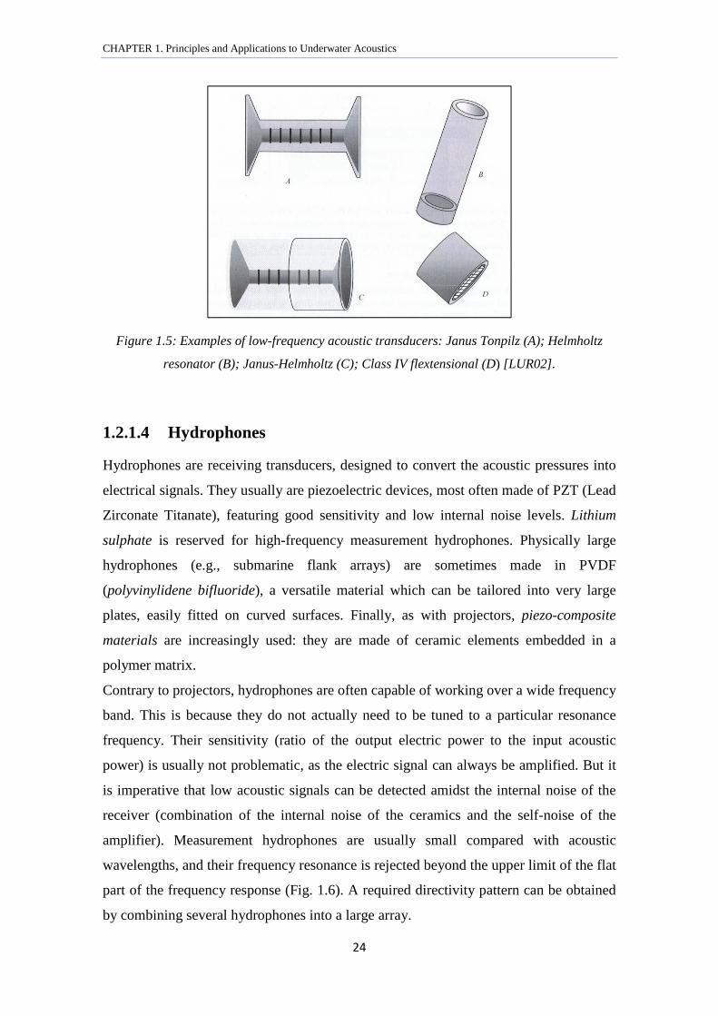
1.2.1.3 Low-frequency transducer
At very low frequencies (below 1 kHz), acoustic source technology encounters serious
limitations. The transducer must be capable of withstanding at the large amplitudes
emitted; and they are very heavy and big.
Several solutions have been proposed (Fig. 1.5) each one being generally adapted to
solve a particular problem. Among them, one can cite:
− The extension of Tonpilz technology to low frequencies with some
modifications. For example, the Janus concept equips the Tonpilz transducer
with two opposing projectors (Fig. 1.5a). This type of solution is particularly
well suited when high transmission levels are required.
− Sources based on the Helmholtz resonator technology. These are commonly
used by oceanographers for acoustic tomography experiments. An open metal
tube is excited at one end by a piezoelectric driver (Fig. 1.5b). The entire
structure resonates at a frequency given by L=λ/4, where L is the length of the
tube. Initially designed for frequencies between 400 Hz and 250Hz, this
solution is simple, robust, low-cost and insensitive to hydrostatic pressure.
CHAPTER 1. Principles and Applications to Underwater Acoustics
23
Unfortunately, it shows poor efficiency, limited power and very narrow
frequency bandwidths.
− A Helmholtz resonator can be coupled with a Janus transducer, leading to the
Janus-Helmholtz concept (Fig. 1.5c). Coupling the resonance of the transducer
with that of the Helmholtz resonator yields a wide bandwidth and is efficient at
the same time. This means that the elasticity inside the resonator cavity must be
increased, using either compliant tubes or a compressible fluid. Initially
designed for military low-frequency active sonars, and usable at great depths,
this concept has been extended to sources used in physical oceanography and
marine seismology.
− Flextensional transducers are also an appealing solution for high-power
applications such as military sonars. They consist of an elastic shell, in which
an electro-acoustic driver is inserted. This is the piezoelectric stack, whose
longitudinal vibrations induce deformations in the radiating shell. The Class IV
type (Fig.1.5d) is the most commonly used: the shell is an elliptical cylinder,
and the ceramic bar is inserted along its main radial axis. These transducers
have a high efficiency at low frequencies, with compact dimensions. However,
they cannot withstand high pressure, as the static deformation of the shell
decouples it from the piezoelectric driver.
− Hydraulic technology has been used for acoustic thermometry experiments
requiring large, broadband transmissions around 60Hz. A hydraulic block,
electrically controlled, moves radiating shells trough a piston. Well suited to
very low frequencies, this transducer concept requires high electric power and
specific cooling devices; it is therefore ill-adapted to autonomous sources.
− Electrodynamic sources similar to aerial loudspeakers can be used to transmit
broadband low-frequency signals. But the levels available are very limited
because of mediocre efficiencies, and it is very difficult to compensate for
hydrostatic pressure below a few metres [LUR02].
CHAPTER 1. Principles and Applications to Underwater Acoustics
24
Figure 1.5: Examples of low-frequency acoustic transducers: Janus Tonpilz (A); Helmholtz
resonator (B); Janus-Helmholtz (C); Class IV flextensional (D) [LUR02].
1.2.1.4 Hydrophones
Hydrophones are receiving transducers, designed to convert the acoustic pressures into
electrical signals. They usually are piezoelectric devices, most often made of PZT (Lead
Zirconate Titanate), featuring good sensitivity and low internal noise levels. Lithium
sulphate is reserved for high-frequency measurement hydrophones. Physically large
hydrophones (e.g., submarine flank arrays) are sometimes made in PVDF
(polyvinylidene bifluoride), a versatile material which can be tailored into very large
plates, easily fitted on curved surfaces. Finally, as with projectors, piezo-composite
materials are increasingly used: they are made of ceramic elements embedded in a
polymer matrix.
Contrary to projectors, hydrophones are often capable of working over a wide frequency
band. This is because they do not actually need to be tuned to a particular resonance
frequency. Their sensitivity (ratio of the output electric power to the input acoustic
power) is usually not problematic, as the electric signal can always be amplified. But it
is imperative that low acoustic signals can be detected amidst the internal noise of the
receiver (combination of the internal noise of the ceramics and the self-noise of the
amplifier). Measurement hydrophones are usually small compared with acoustic
wavelengths, and their frequency resonance is rejected beyond the upper limit of the flat
part of the frequency response (Fig. 1.6). A required directivity pattern can be obtained
by combining several hydrophones into a large array.

CHAPTER 1. Principles and Applications to Underwater Acoustics
25
The same transducer is often used for transmission and reception in many sonar
systems, e.g., single-beam echo sounders, acoustic Doppler current profilers (ADCPs),
sidescan sonars.
Figure 1.6: (Left) Frequency response curve and bandwidth of a transducer. (Right)
Frequency response curve of a hydrophone: the resonance frequency ! is rejected beyond the
effective bandwidth B [LUR02].
1.3 Underwater Acoustics Applications
The use of underwater sounds is a recent technological development and it is now part
of most human activities at sea. Its technology is applied in the oceans, scientifically,
militarily or industrially. The number and type of applications has grown considerably,
and in general, they are used underwater to:
a. “detect” and “locate” obstacles and target; this is the primary function of sonar
systems, mostly for military applications such as anti-submarine warfare and
minehunting, but also used in fisheries;
b. “measure” either the characteristics of the marine environment (seafloor
topography, living organisms, currents and hydrological structures, etc.) or the
location and velocity of an object moving underwater;
c. “transmit” signals, which may be data acquired by underwater scientific
instrumentation, messages between submarines and surface vessels, or
commands to remotely operated systems.
These systems are for the most part active systems, that is, they transmit a characteristic
signal, and this signal will be reflected on a target or transmitted directly to a receiver.
But there are also passive systems, designed to intercept and exploit underwater sounds
coming from the target itself [LUR02].
CHAPTER 1. Principles and Applications to Underwater Acoustics
26
In the following, the main modern applications of underwater acoustics divided in
military and civil applications will be shown briefly.
1.3.1 Military applications
As known, most of the research and industrialization effort in underwater acoustics was
largely linked to military applications. These systems are therefore mostly aimed at
detecting, locating and identifying two types of target namely submarines and mines.
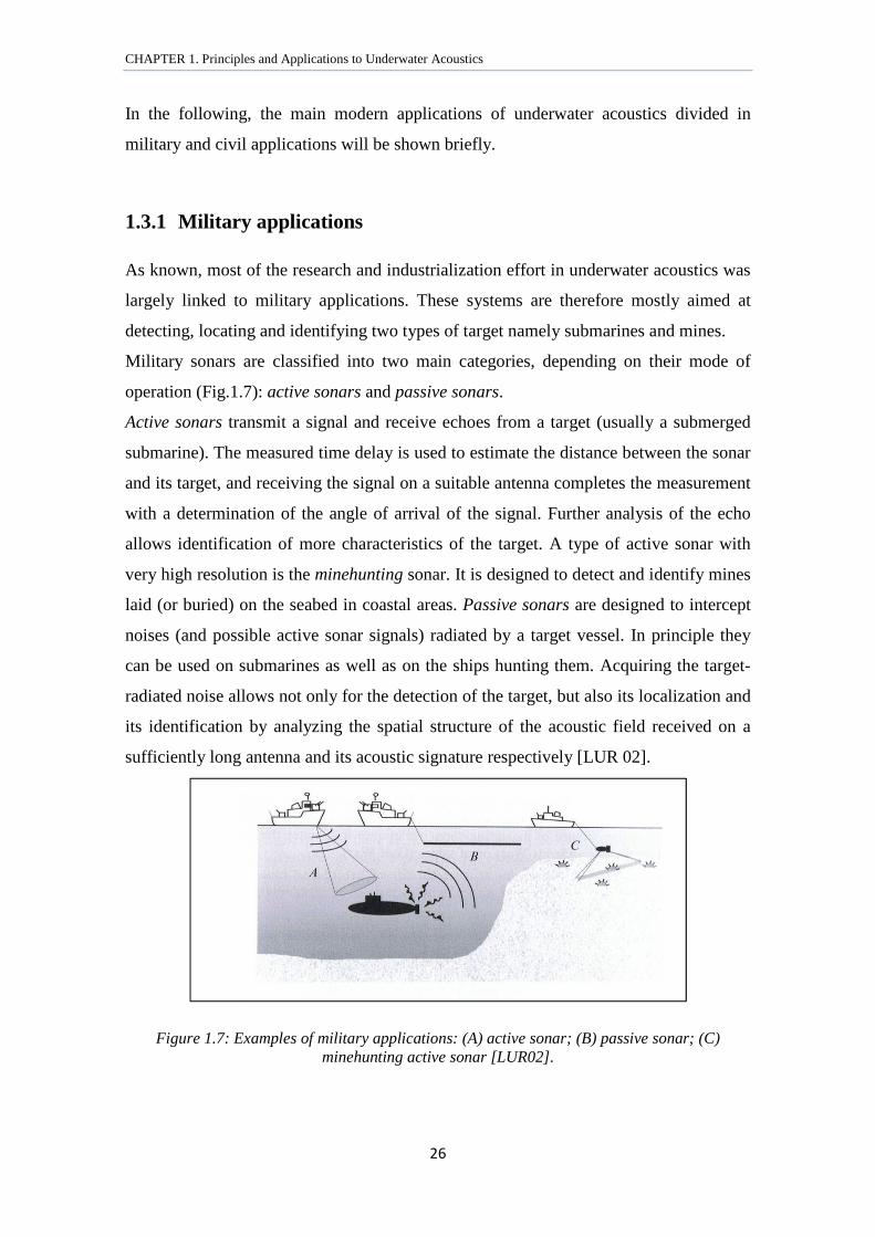
Military sonars are classified into two main categories, depending on their mode of
operation (Fig.1.7): active sonars and passive sonars.
Active sonars transmit a signal and receive echoes from a target (usually a submerged
submarine). The measured time delay is used to estimate the distance between the sonar
and its target, and receiving the signal on a suitable antenna completes the measurement
with a determination of the angle of arrival of the signal. Further analysis of the echo
allows identification of more characteristics of the target. A type of active sonar with
very high resolution is the minehunting sonar. It is designed to detect and identify mines
laid (or buried) on the seabed in coastal areas. Passive sonars are designed to intercept
noises (and possible active sonar signals) radiated by a target vessel. In principle they
can be used on submarines as well as on the ships hunting them. Acquiring the target-
radiated noise allows not only for the detection of the target, but also its localization and
its identification by analyzing the spatial structure of the acoustic field received on a
sufficiently long antenna and its acoustic signature respectively [LUR 02].
Figure 1.7: Examples of military applications: (A) active sonar; (B) passive sonar; (C) minehunting active sonar [LUR02].
CHAPTER 1. Principles and Applications to Underwater Acoustics
27
1.3.2 Civilian applications
Civilian underwater acoustics is a more modest sector of industrial and scientific
activity, but it is highly diverse and growing. It has been, specially, invigorated by the
needs for scientific instrumentation raised by large scientific programmes of
environment study and monitoring, as well as developments in offshore engineering and
industrial fishing. The main categories of systems are: bathymetric sounders, fishery
sounders, sidescan sonars, multibeam sounders, sediment profilers, acoustic
communication systems, acoustic Doppler systems, acoustic tomography networks and
positioning systems (fig.1.8) [LUR 02].
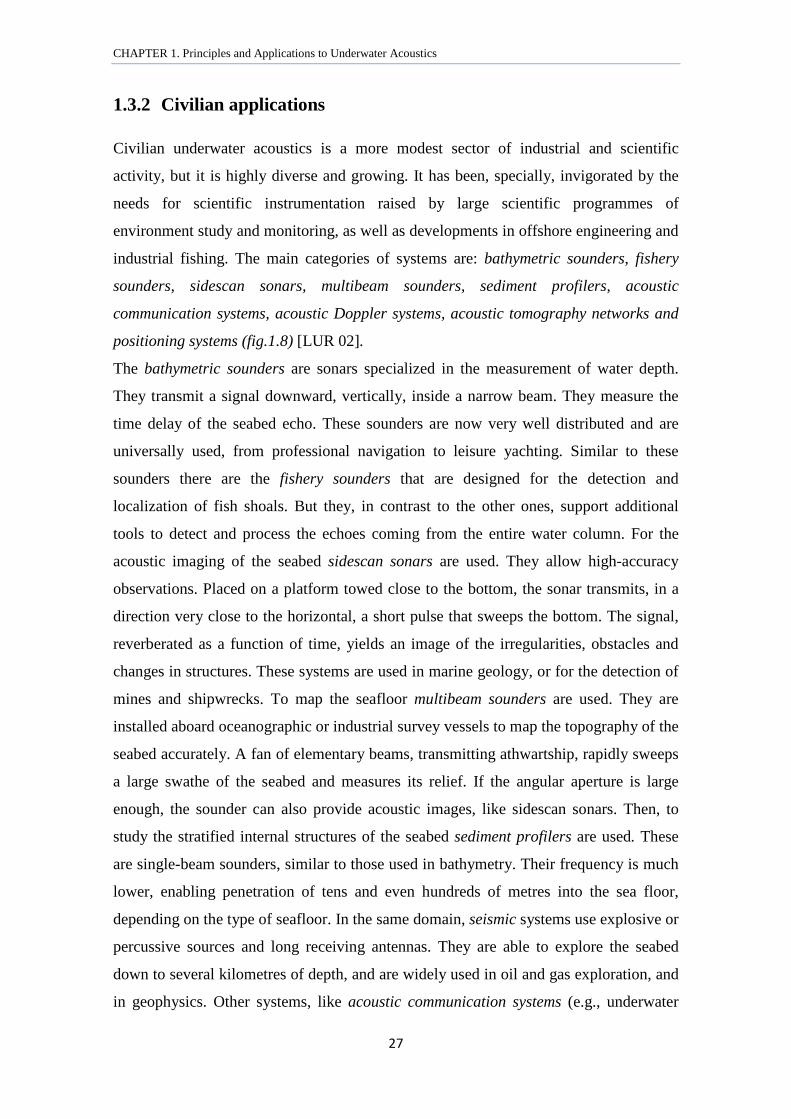
The bathymetric sounders are sonars specialized in the measurement of water depth.
They transmit a signal downward, vertically, inside a narrow beam. They measure the
time delay of the seabed echo. These sounders are now very well distributed and are
universally used, from professional navigation to leisure yachting. Similar to these
sounders there are the fishery sounders that are designed for the detection and
localization of fish shoals. But they, in contrast to the other ones, support additional
tools to detect and process the echoes coming from the entire water column. For the
acoustic imaging of the seabed sidescan sonars are used. They allow high-accuracy
observations. Placed on a platform towed close to the bottom, the sonar transmits, in a
direction very close to the horizontal, a short pulse that sweeps the bottom. The signal,
reverberated as a function of time, yields an image of the irregularities, obstacles and
changes in structures. These systems are used in marine geology, or for the detection of
mines and shipwrecks. To map the seafloor multibeam sounders are used. They are
installed aboard oceanographic or industrial survey vessels to map the topography of the
seabed accurately. A fan of elementary beams, transmitting athwartship, rapidly sweeps
a large swathe of the seabed and measures its relief. If the angular aperture is large
enough, the sounder can also provide acoustic images, like sidescan sonars. Then, to
study the stratified internal structures of the seabed sediment profilers are used. These
are single-beam sounders, similar to those used in bathymetry. Their frequency is much
lower, enabling penetration of tens and even hundreds of metres into the sea floor,
depending on the type of seafloor. In the same domain, seismic systems use explosive or
percussive sources and long receiving antennas. They are able to explore the seabed
down to several kilometres of depth, and are widely used in oil and gas exploration, and
in geophysics. Other systems, like acoustic communication systems (e.g., underwater
CHAPTER 1. Principles and Applications to Underwater Acoustics
28
telephone), beyond their primary use as a phone link, are also used for the transmission
of digital data (e.g., remote control commands, images, results from measurements).
Their performance is limited by the small bandwidths available, and by the difficulties
inherent to underwater propagation. Rates of several kilobits per second are, however,
achievable at distance of several kilometres. To measure the speed of the sonar relative
to a fixed medium or the speed of water relative to a fixed medium instrument using the
frequency shift of echoes acoustic Doppler systems are employed. Instead acoustic
tomography networks, which use fixed transmitters and receivers, are employed to
measure propagation times or amplitude fluctuations to assess the structure of
hydrological perturbations, using speed variations estimates. Last, and very important
for the study developed in this thesis, there are positioning systems. They are used, for
example, for the dynamic anchoring of oil drilling vessels or the tracking of
submersibles or towed platforms. The mobile target is often located by measuring the
time delays for signals coming from several fixed transmitters placed on the bottom
[LUR02]. Different geometries are in fact achievable. In the next section the different
types of this system will be described.
Figure 1.8: Examples of civil applications: (A) bathymetry or fishery sounder; (B) sidescan
sonar; (C) multibeam sounder; (D) data transmission system; (E) acoustic positioning system;
(F) sediment profiler [LUR02].
1.4 Acoustic Positioning
The means available for direct intervention in increasingly deeper waters have steadily
progressed during the last 50 years. The scientific community interested in the deep
ocean wanted dedicated instrumentation that could be used at depths of several
kilometres, and the development of appropriate deployment tools. At the same time, the
CHAPTER 1. Principles and Applications to Underwater Acoustics
29
offshore industry increasingly looked at the possibility of deepwater hydrocarbon
exploitation and shipwreck investigation. All these applications, some of which have
important economic implications, led to the development of the original underwater
acoustic techniques, for the local positioning of ships and submersibles on the one part,
and for the transmission of data on the other. But in this section only the positioning
systems will be delineated.
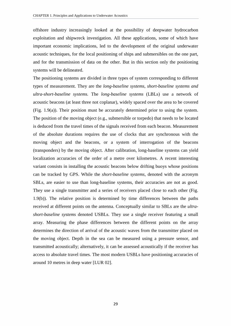
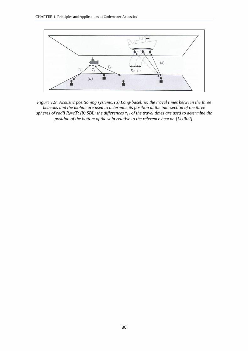
The positioning systems are divided in three types of system corresponding to different
types of measurement. They are the long-baseline systems, short-baseline systems and
ultra-short-baseline systems. The long-baseline systems (LBLs) use a network of
acoustic beacons (at least three not coplanar), widely spaced over the area to be covered
(Fig. 1.9(a)). Their position must be accurately determined prior to using the system.
The position of the moving object (e.g., submersible or torpedo) that needs to be located
is deduced from the travel times of the signals received from each beacon. Measurement
of the absolute durations requires the use of clocks that are synchronous with the
moving object and the beacons, or a system of interrogation of the beacons
(transponders) by the moving object. After calibration, long-baseline systems can yield
localization accuracies of the order of a metre over kilometres. A recent interesting
variant consists in installing the acoustic beacons below drifting buoys whose positions
can be tracked by GPS. While the short-baseline systems, denoted with the acronym
SBLs, are easier to use than long-baseline systems, their accuracies are not as good.
They use a single transmitter and a series of receivers placed close to each other (Fig.
1.9(b)). The relative position is determined by time differences between the paths
received at different points on the antenna. Conceptually similar to SBLs are the ultra-
short-baseline systems denoted USBLs. They use a single receiver featuring a small
array. Measuring the phase differences between the different points on the array
determines the direction of arrival of the acoustic waves from the transmitter placed on
the moving object. Depth in the sea can be measured using a pressure sensor, and
transmitted acoustically; alternatively, it can be assessed acoustically if the receiver has
access to absolute travel times. The most modern USBLs have positioning accuracies of
around 10 metres in deep water [LUR 02].
CHAPTER 1. Principles and Applications to Underwater Acoustics
30
Figure 1.9: Acoustic positioning systems. (a) Long-baseline: the travel times between the three beacons and the mobile are used to determine its position at the intersection of the three
spheres of radii Ri=cT; (b) SBL: the differences "#$ of the travel times are used to determine the position of the bottom of the ship relative to the reference beacon [LUR02].

CHAPTER 2. Acoustic Positioning System in Underwater Neutrino Telescopes
31
Chapter 2
Acoustic Positioning System in Underwater Neutrino
Telescopes
2.1 Underwater Neutrino Telescopes
Lately underwater neutrino telescopes have become important tools of astroparticle
physics since they allow for a new and unique method to observe the Universe.
Neutrinos are stable neutral particles that interact only via the weak force. They can
escape from sources surrounded with dense matter or radiation fields and can traverse
cosmological distances without being absorbed or scattered. This implies that neutrinos
can bring us astrophysical information that other messengers cannot and, open a
potential new window on the Universe [AGE11] This property contrasts to that of other
particles, such as gammas, protons, cosmic rays, etc. that can be absorbed by the cosmic
dust, by the radiation or deviated by the galactic and intergalactic magnetic fields and
then they cannot bring us information about their originating place. On the other hand,
the low interaction cross section of the neutrinos imposes a great challenge for their
detection: only a tiny fraction of incident neutrinos can be observed. To compensate for
this it is necessary to build very large detectors. One way to detect neutrino interactions
can be afforded through the detection of the Cherenkov light emitted by the muon
generated after a neutrino interaction. This particle travels across the detector at speed
greater than the speed of light in water, so generating a faint blue luminescence called
Cherenkov radiation. As said, it is necessary the instrumentation of large volumes of
water (or ice) with several optical sensors in order to detect characteristic signatures of
high energy neutrino interactions. The main elements of a neutrino telescope are
therefore the sensitive optical detectors, usually photomultiplier tubes (PMTs) hosted to
the inner surfaces of pressure-resistant glass spheres named optical modules (OMs),
which collect the light and transforms it into electric signals. The arrival times of the
light collected by optical detectors distributed over a three dimensional array can be
used to reconstruct the muon trajectory, and consequently that of the neutrino, which at
sufficiently high energies are collinear (see Fig. 2.1). The accuracy of reconstruction of

CHAPTER 2. Acoustic Positioning System in Underwater Neut
the muon track depends on the precision in measur
precise knowledge of the positions of the optical detectors. Good time and position
calibration of the detector is therefore of utmost importance to achieve a good angular
resolution. The measurement of the amount of collected light can be
eliminate background events, to improve the muon track reconstruction quality and to
estimate the neutrino energy [
Figure 2.1: Principle of detection of high energy neutrinos
In the deep sea the semi rigid
and maintained vertical by a
under the effect of currents.
effectively reconstruct the muon track is ~10 cm
is needed to monitor the O
system of the detector that must provide the
structures both during the deployment and the operating phases of the telescope
(monitoring of the OMs positions)
detector position in real time, during the
remotely operating vehicle (ROV) operations; during this phase the accuracy needed is
of the order of 1 m. This capability will also be fundamental in
absolute position and pointing direction,
astrophysical source position in the
two main items: (1) a so called
on the seabed in known positions and (2) an arr
rigidly connected to the mechanical structures
CHAPTER 2. Acoustic Positioning System in Underwater Neutrino Telescopes
32
the muon track depends on the precision in measuring the light arrival time and on
precise knowledge of the positions of the optical detectors. Good time and position
calibration of the detector is therefore of utmost importance to achieve a good angular
resolution. The measurement of the amount of collected light can be effectively
eliminate background events, to improve the muon track reconstruction quality and to
estimate the neutrino energy [BIG09].
Principle of detection of high energy neutrinos (~TeV) in a deeptelescope.
semi rigid structures containing the OMs are anchored
maintained vertical by a buoy, and then the top part of the structures
f currents. Since the accuracy required for the position of the OMs to
effectively reconstruct the muon track is ~10 cm, an Acoustic Positioning S
the OM positions continuously. In particular, the APS is a sub
system of the detector that must provide the position of the telescope’s mechanical
structures both during the deployment and the operating phases of the telescope
Ms positions) [CDR08]. The possibility of reconstructing the
position in real time, during the deployment phase, will support
vehicle (ROV) operations; during this phase the accuracy needed is
of the order of 1 m. This capability will also be fundamental in measuring the telescope
absolute position and pointing direction, allowing for the reconstruction of the
source position in the sky. A deep-sea APS is composed of the following
(1) a so called Long Baseline (LBL) of acoustic transceivers, anchored
on the seabed in known positions and (2) an array of acoustic receivers (hydrophones)
rigidly connected to the mechanical structures of the telescope. The positions
The Cherenkov light is
detected by the PMTs
light arrival time and on the
precise knowledge of the positions of the optical detectors. Good time and position
calibration of the detector is therefore of utmost importance to achieve a good angular
effectively used to
eliminate background events, to improve the muon track reconstruction quality and to
deep-sea neutrino
anchored on the seabed
top part of the structures can move
position of the OMs to
Positioning System (APS)
he APS is a sub-
position of the telescope’s mechanical
structures both during the deployment and the operating phases of the telescope
reconstructing the
support safe naval and
vehicle (ROV) operations; during this phase the accuracy needed is
measuring the telescope,
nstruction of the
sea APS is composed of the following
(LBL) of acoustic transceivers, anchored
receivers (hydrophones)
. The positions of the
CHAPTER 2. Acoustic Positioning System in Underwater Neutrino Telescopes
33
hydrophones are evaluated by measuring the difference between the emission time from
sources of known position (LBL acoustic transceivers) and the arrival time at
hydrophones of unknown position; it is possible to reconstruct their tridimensional
location using triangulation techniques [SIM12].
Moreover the acoustic data can be used to monitor ocean noise and to study the acoustic
neutrino detection. It will also allow monitoring of the environment around the detector
and Earth and Sea Science studies: biology, geophysics and oceanography. In fact, other
way to detect a high energy neutrino interaction is through acoustic detection. The basic
idea is that, when the neutrino interacts in water a large amount of the neutrino energy
can be deposited in a small volume of water. This instantaneous water heating produces
a bipolar acoustic pulse, following the second time derivative of the temperature of the
excited medium. The frequency spectrum of the signal is a function of the transverse
spread of the shower, with typical maximum amplitude in the range of few tens kHz.
The acoustic technique could be extremely fruitful because the sound absorption length
is, in this frequency range, of the order of km [RIC04].
The first generations of neutrino telescopes were AMANDA at the South Pole [SPI05],
ANTARES in the Mediterranean Sea [BRU10] and Baikal [AYN06] in the
homonymous Siberian Lake. The target volume of these installations is typically of the
order of 0.01km3, but over the last decade it has been evident that larger detectors are
needed to exploit the scientific potential of neutrino astronomy. For this reason, the
international scientific community has aimed at the construction of km3 scale detectors.
A first km3-size detector is IceCube [HUL11], installed at the South Pole. A new km3-
size detector planned in the Mediterranean Sea is the KM3NeT neutrino telescope
[KM3Nw]. It will surpass IceCube in sensitivity by a substantial factor and complement
it in its field of view. In particular, its field of view will cover the Galactic Center and a
large fraction of the Galactic plane that are hardly visible to IceCube [KAT11].
In the next sections the ANTARES and NEMO detectors will be described and in
particular their APS, since the proposed innovative APS of KM3Net is based on the
experience achieved with these experiments. Moreover the study and development of
the innovative APS of KM3NeT is the main aim of this thesis.
CHAPTER 2. Acoustic Positioning System in Underwater Neutrino Telescopes
34
2.2 Acoustic Positioning System of the ANTARES detectors
ANTARES (Astronomy with a Neutrino Telescope and Abyss environmental
RESearch) is currently the biggest underwater neutrino telescope in the world and is in
operation in the Northern Hemisphere. The main aim of the detector is the search for
high-energy neutrinos of astrophysical origin [AGU11b, ADR11].
The detector is located in the Mediterranean Sea, about 40 km from Toulon, off the
French coast, at a mooring depth of about 2475 m and has a surface area of ~0.1km2. It
consists of 12 lines, anchored to the sea floor by an anchor called a ‘bottom string
socket’ (BSS) at distances of about 60-70 m from each other and kept vertical by buoys.
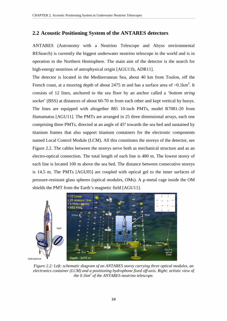
The lines are equipped with altogether 885 10-inch PMTs, model R7081-20 from
Hamamatsu [AGU11]. The PMTs are arranged in 25 three dimensional arrays, each one
comprising three PMTs, directed at an angle of 45º towards the sea bed and sustained by
titanium frames that also support titanium containers for the electronic components
named Local Control Module (LCM). All this constitutes the storeys of the detector, see
Figure 2.2. The cables between the storeys serve both as mechanical structure and as an
electro-optical connection. The total length of each line is 480 m. The lowest storey of
each line is located 100 m above the sea bed. The distance between consecutive storeys
is 14.5 m. The PMTs [AGU05] are coupled with optical gel to the inner surfaces of
pressure-resistant glass spheres (optical modules, OMs). A µ-metal cage inside the OM
shields the PMT from the Earth’s magnetic field [AGU11].
Figure 2.2: Left: schematic diagram of an ANTARES storey carrying three optical modules, an electronics container (LCM) and a positioning hydrophone fixed off-axis. Right: artistic view of
the 0.1km2 of the ANTARES neutrino telescope.
PMT
Hydrophone

CHAPTER 2. Acoustic Positioning System in Underwater Neutrino Telescopes
35
The lines are linked through submersible cables to the Junction Box (JB) that acts as a
fan-out between the main electro-optical cable to shore and the lines.
The detector is complemented by an Instrumentation Line (IL) [AGE11] holding
devices for measurements of environmental parameters as well as tools used by other
scientific communities, including a seismometer. In addition, it includes three acoustic
storeys, which are modified standard storeys replacing the PMTs by acoustic sensors
with custom-designed electronics for signal processing. These three storeys together
with three additional acoustic storeys on Detection Line 12 form the AMADEUS
system that is a basic acoustic system to do long-term studies to check the feasibility of
acoustic ultra-high-energy 1 neutrino detection [LAH12]. The R&D studies for the
construction of the neutrino telescope started in 1996, with the first lines deployed and
connected in 2006. The telescope was completed in May 2008 with the deployment and
connection of the 12th Detection Line [ANTAw].
The telescope also contains timing and position calibration systems, which employ
optical beacons and acoustic transducers installed in each line. The lines are not rigid
structures, so deep-sea currents (typically around 5 cm/s) cause a displacement of the
lines by several metres from vertical position and a rotation of the storeys around their
line axis. Therefore, real time positioning of each line and of all OMs are needed to
ensure optimal track reconstruction with accuracy better than 10 cm (corresponding to
an uncertainty in the travel time of light in water of 0.5 ns). Moreover, the
reconstruction of the muon trajectory and the determination of its energy also require
the knowledge of the OM orientation with a precision of a few degrees. In addition, a
precise absolute orientation of the whole detector has to be achieved in order to find
potential neutrino point-sources in the sky and correlate them with sources of other
messenger particles. To achieve this positioning accuracy during data taking, two
independent systems are incorporated in the detector: an acoustic positioning system
and tiltmeter-compass sensors in each storey.
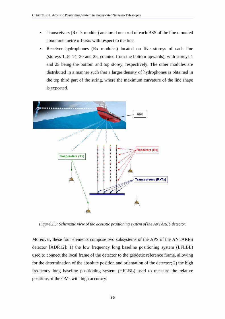
The acoustic positioning system consists of four elements (Fig. 2.3):
• An emitter-receiver acoustic module (AM) located on the ship during the
deployment operation.
• Five autonomous battery-powered transponders located on the sea floor around
the detector area at distances of about 1100-1600 m [ADR12].
1 In the context of neutrino physics typically it refers to neutrinos in excess of 10^18 eV.
CHAPTER 2. Acoustic Positioning System in Underwater Neutrino Telescopes
36
• Transceivers (RxTx module) anchored on a rod of each BSS of the line mounted
about one metre off-axis with respect to the line.
• Receiver hydrophones (Rx modules) located on five storeys of each line
(storeys 1, 8, 14, 20 and 25, counted from the bottom upwards), with storeys 1
and 25 being the bottom and top storey, respectively. The other modules are
distributed in a manner such that a larger density of hydrophones is obtained in
the top third part of the string, where the maximum curvature of the line shape
is expected.
Figure 2.3: Schematic view of the acoustic positioning system of the ANTARES detector.
Moreover, these four elements compose two subsystems of the APS of the ANTARES
detector [ADR12]: 1) the low frequency long baseline positioning system (LFLBL)
used to connect the local frame of the detector to the geodetic reference frame, allowing
for the determination of the absolute position and orientation of the detector; 2) the high
frequency long baseline positioning system (HFLBL) used to measure the relative
positions of the OMs with high accuracy.
AM

CHAPTER 2. Acoustic Positioning System in Underwater Neutrino Telescopes
37
The LFLBL acoustic positioning system is a commercial set of devices provided by the
IXSEA Company [IXSEw]. It is able to measure the travel time of controlled acoustic
pulse between the AM and the autonomous transponders and use the 8-16 kHz
frequency range. The AM is operated on ship and is linked to a time counting electronic
system. The use of acoustic signals at these frequencies allows for long propagation
distances to be measured and for this reason it is suited to determine the position of
ANTARES structures by triangulation from a ship on the sea surface [ADR12].
In the first step, the absolute geodetic positions of the autonomous transponder were
individually determined with an accuracy of better than 1 m before the deployment of
the detector. This result was obtained through several hundred triangulations of the
LFLBL system from a ship positioned by Differential GPS (DGPS). The sound-velocity
profile from the sea surface to the sea floor necessary for this calculation has been
derived from the Chen-Millero formula [CHE77] using sets of temperature and salinity
profiles measured at the ANTARES site.
In the second step, in order to monitor the position of the BSS in real time during the
line deployment, the triangulation of the acoustic travel time measurements between the
transponders on the BSS, the autonomous reference transponders and the AM on the
ship was calculated. The latter is determined with accuracy of a few metres, whereas the
accuracy of the final position of the BSS on the sea bed is about 1 m.
With respect to have a good knowledge of the absolute orientation of the detector, it is
necessary to determine with good accuracy the BSS orientation and depth. The
orientation of the BSS is determined using the compass of a submarine vehicle during
an undersea line connection with an accuracy of about 5º.
The depth of the sea bed at the position of each BSS is measured by a pressure sensor
on the submarine with a precision of about 10 cm. Moreover, the relative positions of
the line anchors are obtained measuring all distances between different transceivers of
the BSSs, which form an auto-calibrated positioning system.
Once the positions of the BSSs are known it is possible to determine the absolute
orientation of the detector using the triangulation between transceivers and
hydrophones, considering that the line remains almost vertical for small speeds of the
sea current (smaller than 2 cm/s).

CHAPTER 2. Acoustic Positioning System in Underwater Neutrino Telescopes
38
In summary, the absolute orientation of the neutrino telescope with respect to the sky,
needed for neutrino astronomy, is obtained using both the absolute positions of the
different line anchors and the BSS to BSS relative positions [ADR12].
The HFLBL acoustic positioning system was developed and constructed by the
company GENISEA/ECA [ECAw] for the relative positioning of the detector strings.
The method used is to measure the travel time of 40-60 kHz acoustic pulses between
receiving hydrophones placed along the string and emitters fixed at the bottom of each
line [KEL07]. Electronic boards manage the settings of the system, for emission,
detection, filtering and recording. The 3D position of each hydrophone is then obtained
by triangulation from the travel times between the hydrophone and each fixed emitter
knowing the sound velocity profile. In fact, there are several sound velocity profilers
located throughout the ANTARES detector, which measure the sound velocity profile
continuously. The positions of all hydrophones and transducers are then computed from
distances using triangulation principle based on a least-mean square minimization.
Measurements for the line shape reconstruction are performed every 2 minutes, which is
enough since the motion of the lines is due to slow counts.
The other independent system incorporated in the detector, as mentioned above, is the
Tiltmeter-Compass System (TCS). It consists of a commercial TCM2 board,
manufactured by PNI Sensor Corporation [PNICw, ADR12], that measures the
inclination of the storey with respect to the horizontal plane in two perpendicular axes
(pitch and roll). It is installed in the electronics module of each storey and it is based on
the movement of a fluid in the sensors due to the inclination of the storey. The absolute
orientation of the TCM2 (heading, i. e., rotation around line axis) also has to be
measured. For this reason three flux tube magnetic sensors measure the Earth magnetic
field in three perpendicular local directions (x, y, z) of the TCM2 frame [ADR12].
The range of measurement for the tiltmeters is ±20º on 2 perpendicular axes (roll and
pitch), with an accuracy of 0.2º, while the compasses measure 360º of heading at a
resolution of 1º. Data is read out from the TCM2 device every 2 minutes and is used in
conjunction with the APS during the line fit [BRO09].
2.3 NEMO Acoustic Positioning System
The NEMO (NEutrino Mediterranean Observatory) Collaboration was set up in 1998
with the aim to carry out the necessary R&D towards a km3 neutrino telescope in the
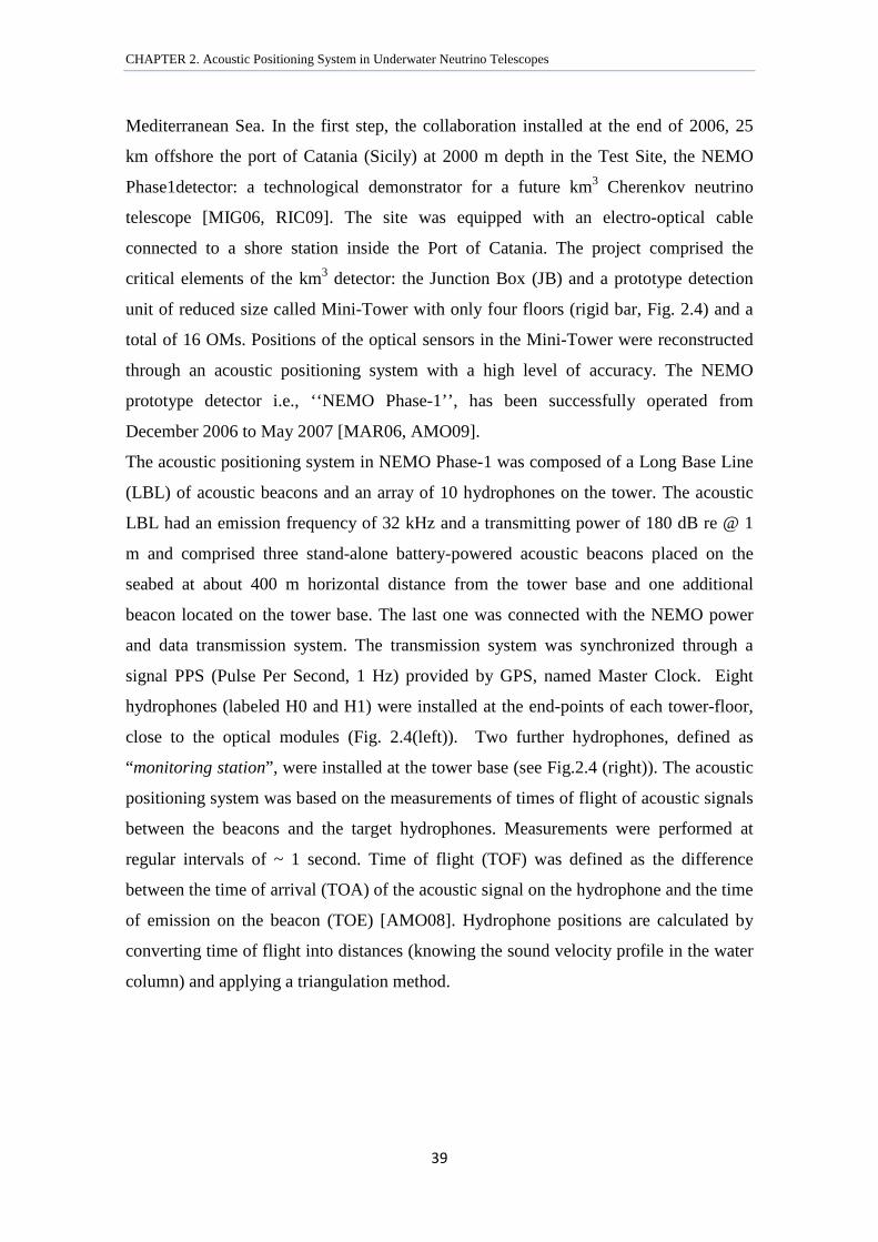
CHAPTER 2. Acoustic Positioning System in Underwater Neutrino Telescopes
39
Mediterranean Sea. In the first step, the collaboration installed at the end of 2006, 25
km offshore the port of Catania (Sicily) at 2000 m depth in the Test Site, the NEMO
Phase1detector: a technological demonstrator for a future km3 Cherenkov neutrino
telescope [MIG06, RIC09]. The site was equipped with an electro-optical cable
connected to a shore station inside the Port of Catania. The project comprised the
critical elements of the km3 detector: the Junction Box (JB) and a prototype detection
unit of reduced size called Mini-Tower with only four floors (rigid bar, Fig. 2.4) and a
total of 16 OMs. Positions of the optical sensors in the Mini-Tower were reconstructed
through an acoustic positioning system with a high level of accuracy. The NEMO
prototype detector i.e., ‘‘NEMO Phase-1’’, has been successfully operated from
December 2006 to May 2007 [MAR06, AMO09].
The acoustic positioning system in NEMO Phase-1 was composed of a Long Base Line
(LBL) of acoustic beacons and an array of 10 hydrophones on the tower. The acoustic
LBL had an emission frequency of 32 kHz and a transmitting power of 180 dB re @ 1
m and comprised three stand-alone battery-powered acoustic beacons placed on the
seabed at about 400 m horizontal distance from the tower base and one additional
beacon located on the tower base. The last one was connected with the NEMO power
and data transmission system. The transmission system was synchronized through a
signal PPS (Pulse Per Second, 1 Hz) provided by GPS, named Master Clock. Eight
hydrophones (labeled H0 and H1) were installed at the end-points of each tower-floor,
close to the optical modules (Fig. 2.4(left)). Two further hydrophones, defined as
“monitoring station”, were installed at the tower base (see Fig.2.4 (right)). The acoustic
positioning system was based on the measurements of times of flight of acoustic signals
between the beacons and the target hydrophones. Measurements were performed at
regular intervals of ~ 1 second. Time of flight (TOF) was defined as the difference
between the time of arrival (TOA) of the acoustic signal on the hydrophone and the time
of emission on the beacon (TOE) [AMO08]. Hydrophone positions are calculated by
converting time of flight into distances (knowing the sound velocity profile in the water
column) and applying a triangulation method.
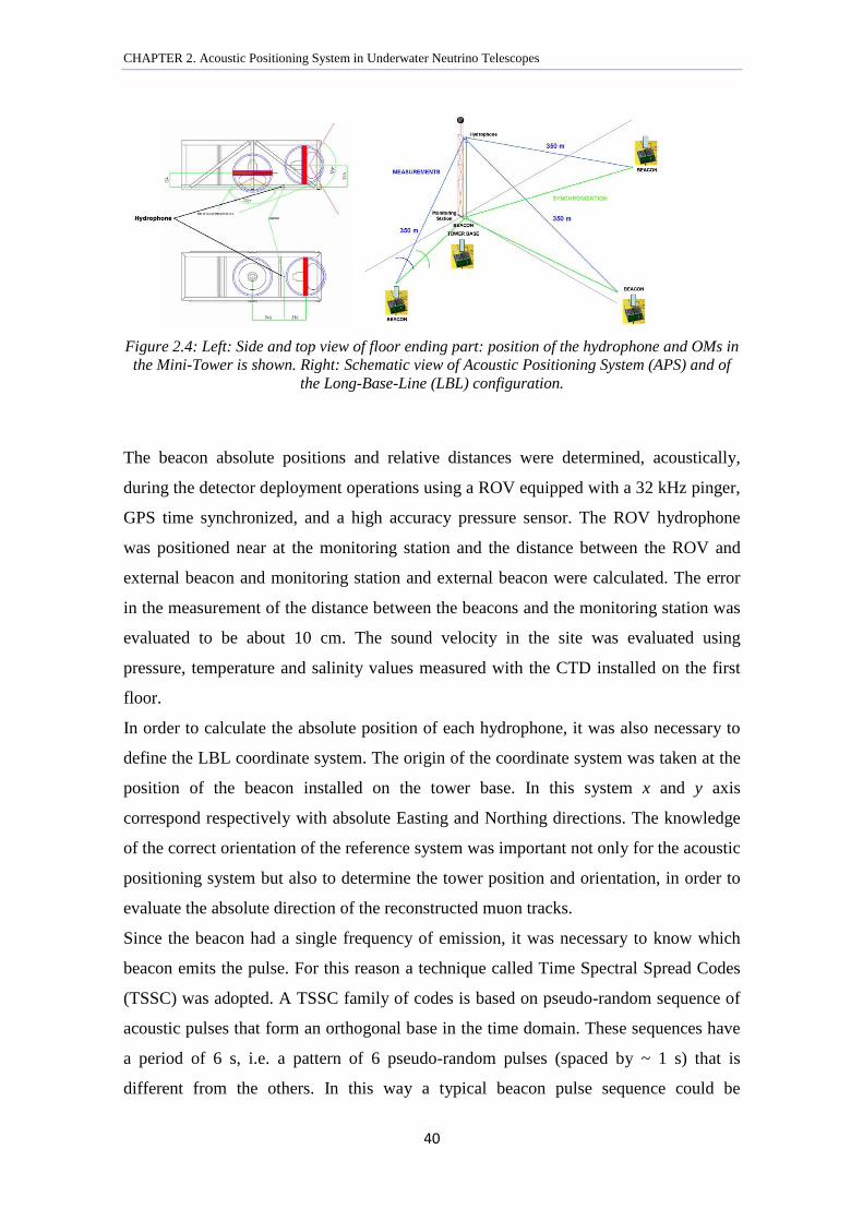
CHAPTER 2. Acoustic Positioning System in Underwater Neutrino Telescopes
40
Figure 2.4: Left: Side and top view of floor ending part: position of the hydrophone and OMs in the Mini-Tower is shown. Right: Schematic view of Acoustic Positioning System (APS) and of
the Long-Base-Line (LBL) configuration.
The beacon absolute positions and relative distances were determined, acoustically,
during the detector deployment operations using a ROV equipped with a 32 kHz pinger,
GPS time synchronized, and a high accuracy pressure sensor. The ROV hydrophone
was positioned near at the monitoring station and the distance between the ROV and
external beacon and monitoring station and external beacon were calculated. The error
in the measurement of the distance between the beacons and the monitoring station was
evaluated to be about 10 cm. The sound velocity in the site was evaluated using
pressure, temperature and salinity values measured with the CTD installed on the first
floor.
In order to calculate the absolute position of each hydrophone, it was also necessary to
define the LBL coordinate system. The origin of the coordinate system was taken at the
position of the beacon installed on the tower base. In this system x and y axis
correspond respectively with absolute Easting and Northing directions. The knowledge
of the correct orientation of the reference system was important not only for the acoustic
positioning system but also to determine the tower position and orientation, in order to
evaluate the absolute direction of the reconstructed muon tracks.
Since the beacon had a single frequency of emission, it was necessary to know which
beacon emits the pulse. For this reason a technique called Time Spectral Spread Codes
(TSSC) was adopted. A TSSC family of codes is based on pseudo-random sequence of
acoustic pulses that form an orthogonal base in the time domain. These sequences have
a period of 6 s, i.e. a pattern of 6 pseudo-random pulses (spaced by ~ 1 s) that is
different from the others. In this way a typical beacon pulse sequence could be
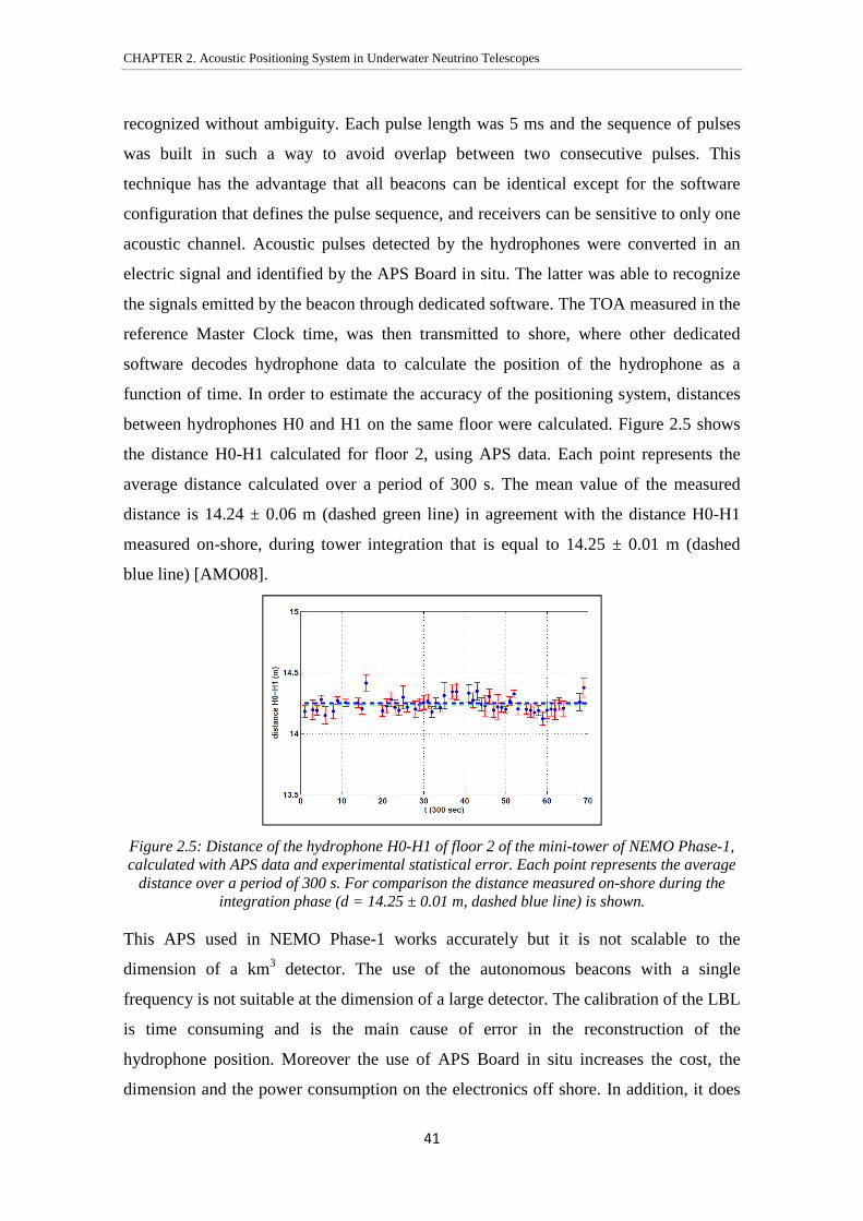
CHAPTER 2. Acoustic Positioning System in Underwater Neutrino Telescopes
41
recognized without ambiguity. Each pulse length was 5 ms and the sequence of pulses
was built in such a way to avoid overlap between two consecutive pulses. This
technique has the advantage that all beacons can be identical except for the software
configuration that defines the pulse sequence, and receivers can be sensitive to only one
acoustic channel. Acoustic pulses detected by the hydrophones were converted in an
electric signal and identified by the APS Board in situ. The latter was able to recognize
the signals emitted by the beacon through dedicated software. The TOA measured in the
reference Master Clock time, was then transmitted to shore, where other dedicated
software decodes hydrophone data to calculate the position of the hydrophone as a
function of time. In order to estimate the accuracy of the positioning system, distances
between hydrophones H0 and H1 on the same floor were calculated. Figure 2.5 shows
the distance H0-H1 calculated for floor 2, using APS data. Each point represents the
average distance calculated over a period of 300 s. The mean value of the measured
distance is 14.24 ± 0.06 m (dashed green line) in agreement with the distance H0-H1
measured on-shore, during tower integration that is equal to 14.25 ± 0.01 m (dashed
blue line) [AMO08].
Figure 2.5: Distance of the hydrophone H0-H1 of floor 2 of the mini-tower of NEMO Phase-1, calculated with APS data and experimental statistical error. Each point represents the average
distance over a period of 300 s. For comparison the distance measured on-shore during the integration phase (d = 14.25 ± 0.01 m, dashed blue line) is shown.
This APS used in NEMO Phase-1 works accurately but it is not scalable to the
dimension of a km3 detector. The use of the autonomous beacons with a single
frequency is not suitable at the dimension of a large detector. The calibration of the LBL
is time consuming and is the main cause of error in the reconstruction of the
hydrophone position. Moreover the use of APS Board in situ increases the cost, the
dimension and the power consumption on the electronics off shore. In addition, it does

CHAPTER 2. Acoustic Positioning System in Underwater Neutrino Telescopes
42
not allow for changes of the analysis data system after the deployment. For this reason
the Collaboration NEMO has developed a new APS that will be described in the
following.
As the next step, the collaboration will install, in 2012, the NEMO Phase II
demonstrator off-shore Capo Passero (Sourth-East Sicily) at a depth of 3500 m. It is a
prototype of a detection unit of a neutrino telescope consisting in a semi-rigid vertical
structure called towers. The towers are composed of 8 horizontal 8 m-long frames
(named floors) made of marine grade aluminum tensioned by a system of ropes. The
prototype will be about 420 m high and will be anchored on the sea bed and kept
vertical by buoy on the top. The distance between floors is 40 m, while that between the
anchor and the lowermost floor is about 100 m. Each floor has two optical modules at
either end, (resulting in a total of 32 optical modules in the tower), one looking
vertically downwards and the other horizontally outwards. Each floor furthermore hosts
instrumentation for positioning and environmental parameter monitoring. The
positioning of the detector is provided by a 3D array of 18 acoustic sensors installed at
both ends of each floor and at the base of the detector (monitoring station). In addition,
four autonomous acoustic beacons will be anchored on the sea bed at distance of about
500 m from the base of the tower and one powered beacon will be located at the base of
the tower (Fig. 2.6). The beacons, which are manufactured by ACSA [ACSAw], emit
known packets of sinusoidal signals of 32 kHz, 5ms duration, 180 dB re 1 µPa at 1 m
transmitting power. Moreover, they constitute the basic points to define a Cartesian
reference system of orthogonal axes related to the so-called long baseline (LBL) that
will permit to calculate the position of each hydrophone [SIM11].
Figure 2.6: Schematic view of the acoustic positioning system of the NEMO Phase II detector. The positioning of the detector is based on the measurement of the time of flight of acoustic

CHAPTER 2. Acoustic Positioning System in Underwater Neutrino Telescopes
43
signals between beacons of a long baseline acoustic system, anchored on the sea-floor, and acoustic receivers acting as targets, rigidly connected to the mechanical structures of the
detector.
The receiver array is composed of: 14 high sensitivity and broadband (10 Hz-70 kHz)
hydrophones SMID, provided by INFN (Italy); 2 free flooded rings (FFR) hydrophones
Sensor Techonolgy Ltd SX-30, provided by UPV (Spain) in collaboration with CPPM-
CNRS (France)-proposed for possible use in the KM3NeT long-baseline- that will be
described in the next chapters and is the main subject of this thesis; 2 custom piezo-
sensors developed by ECAP (Germany), that will be installed in special Opto-Acoustic
Modules.
The acoustic beacons will be installed during the deployment of the detector. Their
absolute positions and relative distances will be determined, acoustically, during the
detector deployment operations using a ROV (remotely operated vehicle) equipped with
a USBL (ultrashort baseline) positioning system [VIO12].
The hydrophone positions will be calculated by accurate TDoA (Time Difference of
Arrival) measurement between beacon signal emission (start-time) and hydrophone
signal reception (stop-time) with an expected accuracy better than 10 cm [SIM11].
Additionally, there will be in the anchor of the tower the prototype of a transceiver,
acting as emitter, consisting of a free flooded ring (FFR) transducer and the associated
electronics, the Sound Emission Board (SEB). This prototype will be fully explained in
the next chapters.
Naturally, the NEMO Phase II tower will be equipped as well with data acquisition and
transmission electronics, power supply and electro-optical cabling and environmental
probes (2 CTDs, Conductivity-Depth-Temperature, 1 current meter, 1 light transmission
meter).
Contrarily to previous acoustic positioning systems developed, for NEMO Phase I
[AMO09] or ANTARES [ARD09] detectors, in NEMO Phase II the sensors’ data
acquisition system is fully integrated with the detector data transport system and is
based on the “all data to shore” philosophy. Furthermore the structure design permits
assembly and deployment in a compact configuration, and unfurling on the sea bottom
under the pull provided by the buoy. In Figure 2.7 the mechanical scheme of the NEMO
tower and a view of the NEMO Phase-2 site are shown. Differently from the one-
dimensional strings of OMs (e.g., ANTARES [ANTAw]), the tower allows for
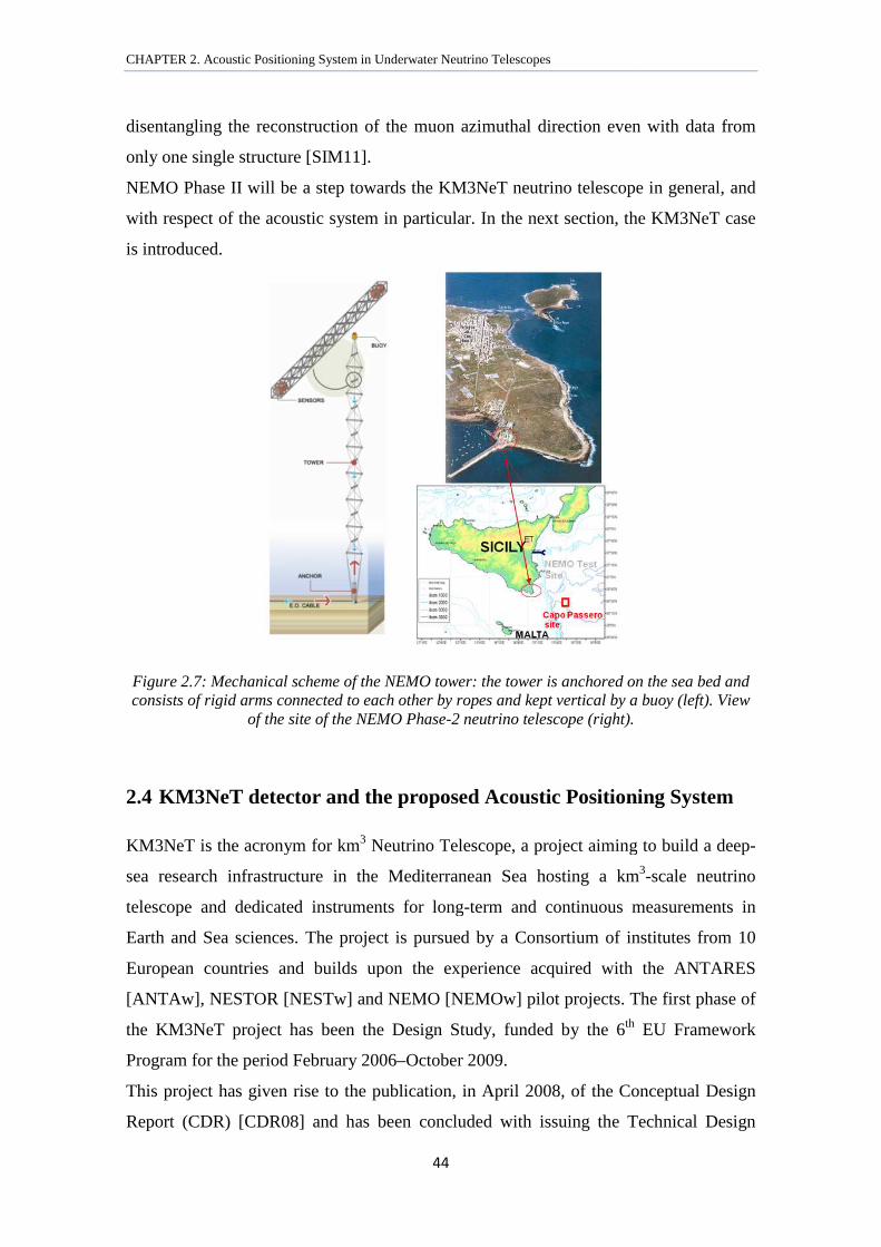
CHAPTER 2. Acoustic Positioning System in Underwater Neut
disentangling the reconstruction
only one single structure [SIM11]
NEMO Phase II will be a step towards the
with respect of the acoustic system
is introduced.
Figure 2.7: Mechanical scheme of the consists of rigid arms connected to each other by ropes and kept vertical by a buoy (left).
of the site of the
2.4 KM3NeT detector and the proposed
KM3NeT is the acronym for km
sea research infrastructure in the Mediterranean Sea hosting a km
telescope and dedicated instruments for long
Earth and Sea sciences. The project is pursued by a
European countries and builds upon
[ANTAw], NESTOR [NESTw]
the KM3NeT project has been
Program for the period February 2006
This project has given rise to the publication, in April 2008, of
Report (CDR) [CDR08] and has been
CHAPTER 2. Acoustic Positioning System in Underwater Neutrino Telescopes
44
reconstruction of the muon azimuthal direction even with data from
[SIM11].
NEMO Phase II will be a step towards the KM3NeT neutrino telescope in general, and
acoustic system in particular. In the next section, the KM3NeT case
Mechanical scheme of the NEMO tower: the tower is anchored on the sea bedof rigid arms connected to each other by ropes and kept vertical by a buoy (left).
site of the NEMO Phase-2 neutrino telescope (right).
detector and the proposed Acoustic Positioning
acronym for km3 Neutrino Telescope, a project aiming
sea research infrastructure in the Mediterranean Sea hosting a km
telescope and dedicated instruments for long-term and continuous measurements in
The project is pursued by a Consortium of institutes from 10
builds upon the experience acquired with the
[NESTw] and NEMO [NEMOw] pilot projects. The fir
the KM3NeT project has been the Design Study, funded by the 6th
for the period February 2006–October 2009.
has given rise to the publication, in April 2008, of the Conceptual Design
and has been concluded with issuing the Technical Design
of the muon azimuthal direction even with data from
KM3NeT neutrino telescope in general, and
, the KM3NeT case
on the sea bed and of rigid arms connected to each other by ropes and kept vertical by a buoy (left). View
ositioning System
ing to build a deep-
sea research infrastructure in the Mediterranean Sea hosting a km3-scale neutrino
term and continuous measurements in
of institutes from 10
with the ANTARES
The first phase of
EU Framework
Conceptual Design
Technical Design
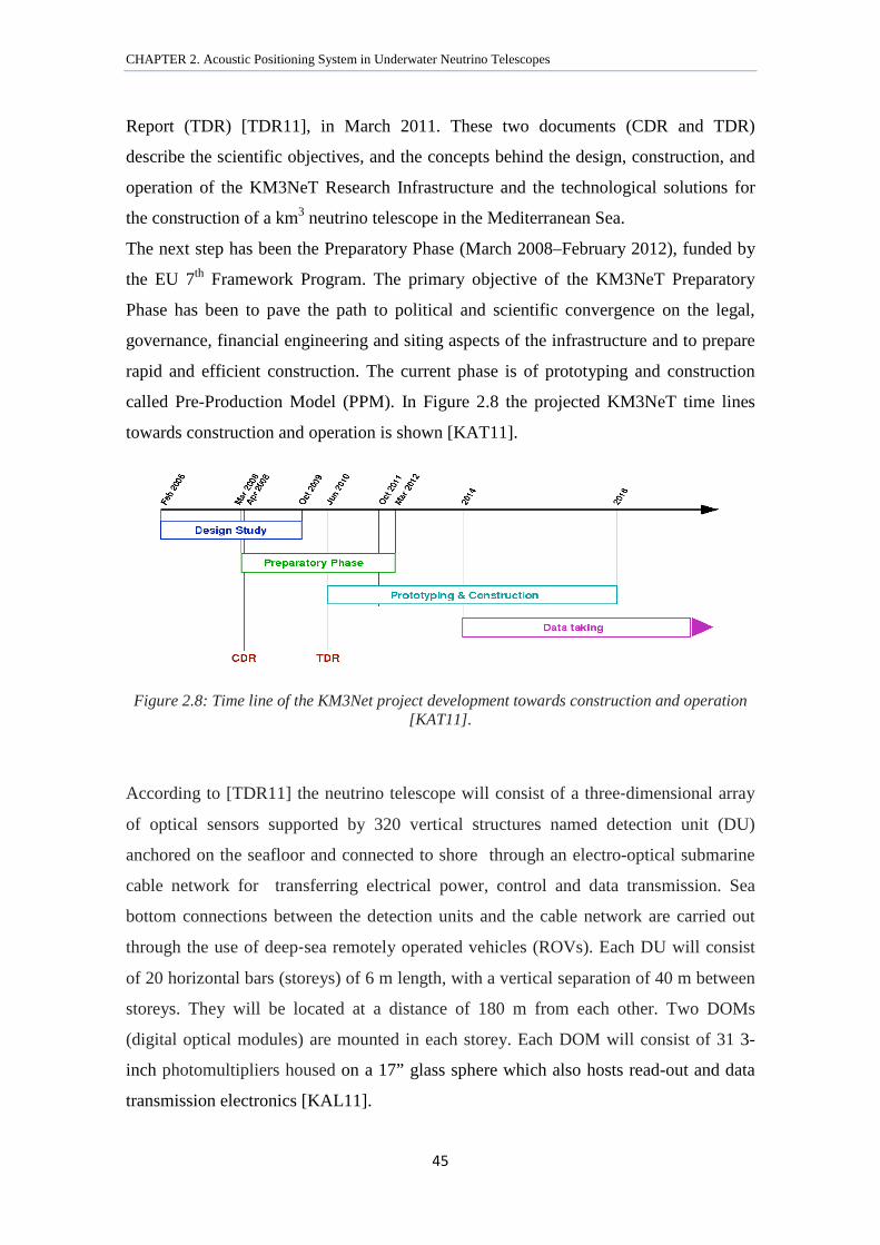
CHAPTER 2. Acoustic Positioning System in Underwater Neutrino Telescopes
45
Report (TDR) [TDR11], in March 2011. These two documents (CDR and TDR)
describe the scientific objectives, and the concepts behind the design, construction, and
operation of the KM3NeT Research Infrastructure and the technological solutions for
the construction of a km3 neutrino telescope in the Mediterranean Sea.
The next step has been the Preparatory Phase (March 2008–February 2012), funded by
the EU 7th Framework Program. The primary objective of the KM3NeT Preparatory
Phase has been to pave the path to political and scientific convergence on the legal,
governance, financial engineering and siting aspects of the infrastructure and to prepare
rapid and efficient construction. The current phase is of prototyping and construction
called Pre-Production Model (PPM). In Figure 2.8 the projected KM3NeT time lines
towards construction and operation is shown [KAT11].
Figure 2.8: Time line of the KM3Net project development towards construction and operation [KAT11].
According to [TDR11] the neutrino telescope will consist of a three‐dimensional array
of optical sensors supported by 320 vertical structures named detection unit (DU)
anchored on the seafloor and connected to shore through an electro-optical submarine
cable network for transferring electrical power, control and data transmission. Sea
bottom connections between the detection units and the cable network are carried out
through the use of deep‐sea remotely operated vehicles (ROVs). Each DU will consist
of 20 horizontal bars (storeys) of 6 m length, with a vertical separation of 40 m between
storeys. They will be located at a distance of 180 m from each other. Two DOMs
(digital optical modules) are mounted in each storey. Each DOM will consist of 31 3-
inch photomultipliers housed on a 17” glass sphere which also hosts read-out and data
transmission electronics [KAL11].
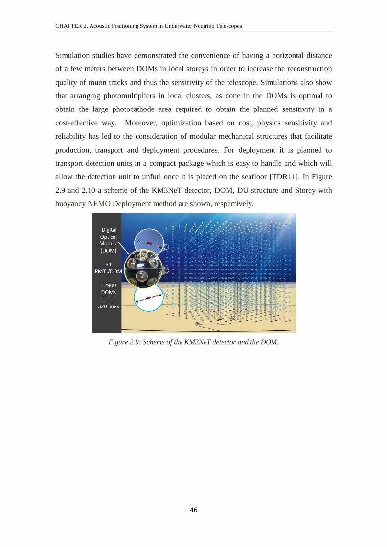
CHAPTER 2. Acoustic Positioning System in Underwater Neutrino Telescopes
46
Simulation studies have demonstrated the convenience of having a horizontal distance
of a few meters between DOMs in local storeys in order to increase the reconstruction
quality of muon tracks and thus the sensitivity of the telescope. Simulations also show
that arranging photomultipliers in local clusters, as done in the DOMs is optimal to
obtain the large photocathode area required to obtain the planned sensitivity in a
cost‐effective way. Moreover, optimization based on cost, physics sensitivity and
reliability has led to the consideration of modular mechanical structures that facilitate
production, transport and deployment procedures. For deployment it is planned to
transport detection units in a compact package which is easy to handle and which will
allow the detection unit to unfurl once it is placed on the seafloor [TDR11]. In Figure
2.9 and 2.10 a scheme of the KM3NeT detector, DOM, DU structure and Storey with
buoyancy NEMO Deployment method are shown, respectively.
Figure 2.9: Scheme of the KM3NeT detector and the DOM.
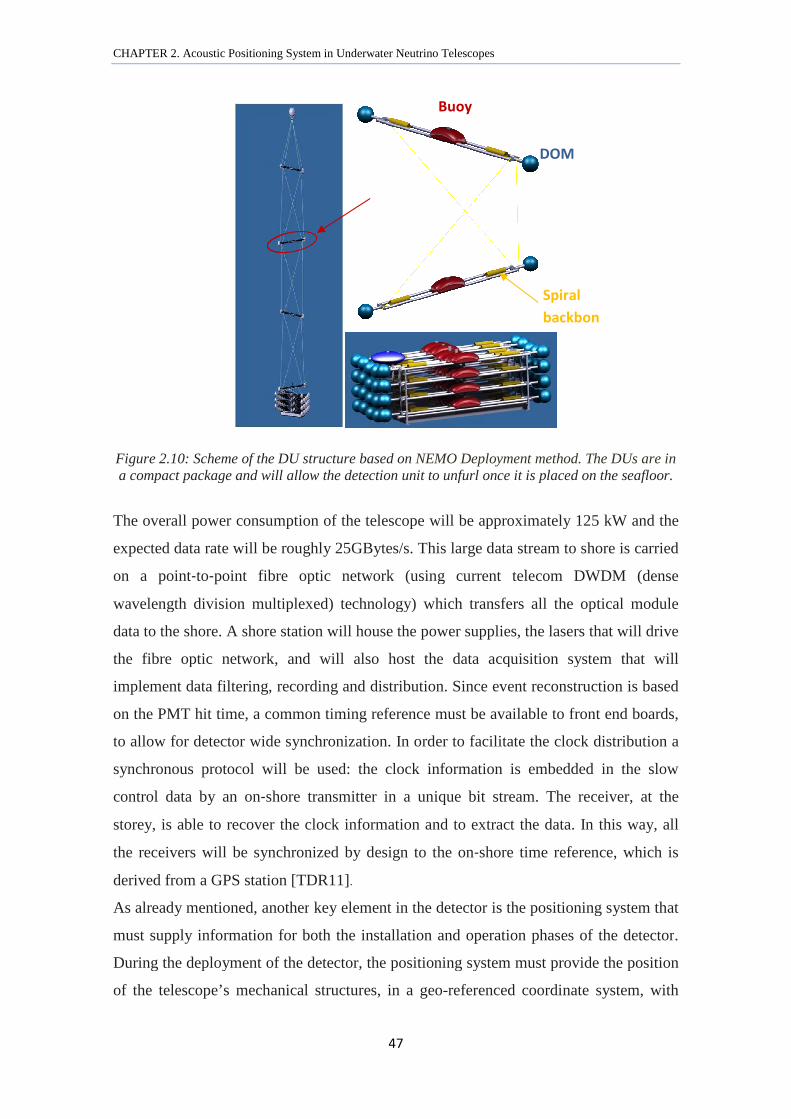
CHAPTER 2. Acoustic Positioning System in Underwater Neut
Figure 2.10: Scheme of the DU structure a compact package and will allow the detection unit to unfurl once it is placed on the seafloor.
The overall power consumption of the telescope
expected data rate will be roughly 25GBytes/s. This large data stream to shore is carried
on a point‐to‐point fibre optic network
wavelength division multiplexed) technology)
data to the shore. A shore station will house the power supplies, the lasers that will drive
the fibre optic network, and will also host the data acquisition system that will
implement data filtering, recording and distribution.
on the PMT hit time, a common timing reference must be available to front end boards,
to allow for detector wide synchronization. In order to facilitate the clock distribution a
synchronous protocol will be used: the clo
control data by an on‐shore transmitter in a unique bit stream. The receiver, at the
storey, is able to recover the clock
the receivers will be synchronized by des
derived from a GPS station
As already mentioned, another
must supply information for both the installation and
During the deployment of the detector, the positioning system must provide the position
of the telescope’s mechanical structures, in a geo
CHAPTER 2. Acoustic Positioning System in Underwater Neutrino Telescopes
47
: Scheme of the DU structure based on NEMO Deployment method. The DUs are ina compact package and will allow the detection unit to unfurl once it is placed on the seafloor.
The overall power consumption of the telescope will be approximately 125 kW and the
expected data rate will be roughly 25GBytes/s. This large data stream to shore is carried
fibre optic network (using current telecom DWDM (dense
wavelength division multiplexed) technology) which transfers all the optical module
A shore station will house the power supplies, the lasers that will drive
the fibre optic network, and will also host the data acquisition system that will
implement data filtering, recording and distribution. Since event reconstruction is based
on the PMT hit time, a common timing reference must be available to front end boards,
detector wide synchronization. In order to facilitate the clock distribution a
synchronous protocol will be used: the clock information is embedded in the slow
shore transmitter in a unique bit stream. The receiver, at the
storey, is able to recover the clock information and to extract the data. In this way, all
the receivers will be synchronized by design to the on‐shore time reference, which is
derived from a GPS station [TDR11].
another key element in the detector is the positioning system
information for both the installation and operation phases of the detector
During the deployment of the detector, the positioning system must provide the position
of the telescope’s mechanical structures, in a geo-referenced coordinate system, with
Buoy
DOM
Spiral
backbon
NEMO Deployment method. The DUs are in a compact package and will allow the detection unit to unfurl once it is placed on the seafloor.
approximately 125 kW and the
expected data rate will be roughly 25GBytes/s. This large data stream to shore is carried
(using current telecom DWDM (dense
all the optical module
A shore station will house the power supplies, the lasers that will drive
the fibre optic network, and will also host the data acquisition system that will
Since event reconstruction is based
on the PMT hit time, a common timing reference must be available to front end boards,
detector wide synchronization. In order to facilitate the clock distribution a
is embedded in the slow
shore transmitter in a unique bit stream. The receiver, at the
and to extract the data. In this way, all
shore time reference, which is
he positioning system that
operation phases of the detector.
During the deployment of the detector, the positioning system must provide the position
nate system, with
DOM
Spiral
backbon
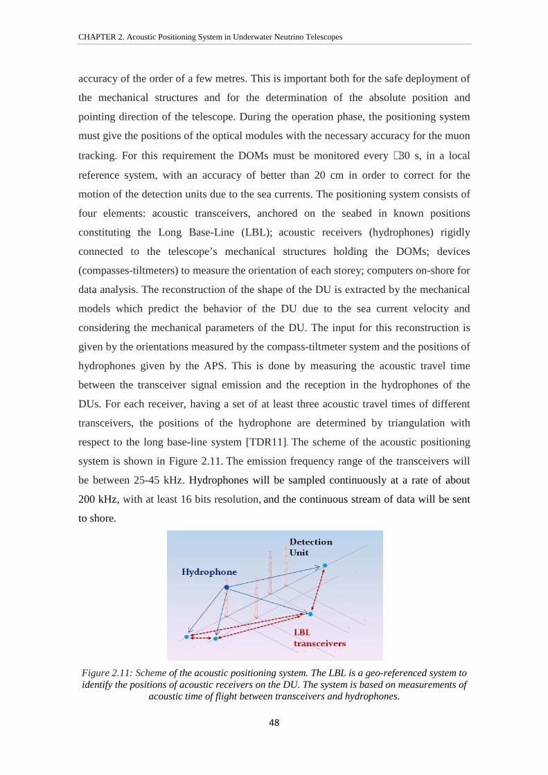
CHAPTER 2. Acoustic Positioning System in Underwater Neutrino Telescopes
48
accuracy of the order of a few metres. This is important both for the safe deployment of
the mechanical structures and for the determination of the absolute position and
pointing direction of the telescope. During the operation phase, the positioning system
must give the positions of the optical modules with the necessary accuracy for the muon
tracking. For this requirement the DOMs must be monitored every ∼30 s, in a local
reference system, with an accuracy of better than 20 cm in order to correct for the
motion of the detection units due to the sea currents. The positioning system consists of
four elements: acoustic transceivers, anchored on the seabed in known positions
constituting the Long Base-Line (LBL); acoustic receivers (hydrophones) rigidly
connected to the telescope’s mechanical structures holding the DOMs; devices
(compasses-tiltmeters) to measure the orientation of each storey; computers on-shore for
data analysis. The reconstruction of the shape of the DU is extracted by the mechanical
models which predict the behavior of the DU due to the sea current velocity and
considering the mechanical parameters of the DU. The input for this reconstruction is
given by the orientations measured by the compass-tiltmeter system and the positions of
hydrophones given by the APS. This is done by measuring the acoustic travel time
between the transceiver signal emission and the reception in the hydrophones of the
DUs. For each receiver, having a set of at least three acoustic travel times of different
transceivers, the positions of the hydrophone are determined by triangulation with
respect to the long base-line system [TDR11]. The scheme of the acoustic positioning
system is shown in Figure 2.11. The emission frequency range of the transceivers will
be between 25-45 kHz. Hydrophones will be sampled continuously at a rate of about
200 kHz, with at least 16 bits resolution, and the continuous stream of data will be sent
to shore.
Figure 2.11: Scheme of the acoustic positioning system. The LBL is a geo-referenced system to identify the positions of acoustic receivers on the DU. The system is based on measurements of
acoustic time of flight between transceivers and hydrophones.

CHAPTER 2. Acoustic Positioning System in Underwater Neutrino Telescopes
49
The KM3NeT positioning system design is based on the experience of the systems
developed for ANTARES and NEMO, but with a better accuracy in the time
synchronization between transceivers and receivers and the implementation of all data
to shore approach, that is all acquired data will be sent to shore for next analysis. It is
fully integrated with the detector electronics. The components are commercially
available and have been tested to 3500 m depth by the pilot projects [TDR11]. Test on
the transceivers and hydrophones are currently conducted. The transceiver in use are
the free flooded ring ceramic transducer (FFR) model SX30 from Sensortech Ltd,
Canada connected to a Sound Emission Board used when it acts as a beacon. They
permit to obtain both optimal transmission and reception voltage response to build
efficient LBL transceivers [LAR12] and will be described in detail in the next chapters.
Acoustic receivers will be installed on each storey of the DU, as mentioned above, and
promising options are the use of the SMID hydrophones, the FFR transducers acting as
receivers and/or a piezoelectric sensor directly glued inside the glass sphere of the
DOM. These different options will be investigated on the KM3NeT Pre-Production
Model test.
Both the acoustic receivers of the DUs and the LBL transceivers are synchronous and
phased with respect to the master clock time signal transmitted from shore. This set-up
allows also for the use of acoustic data for studies of acoustic neutrino detection and
searches for acoustic and optical coincidences. It will also allow for monitoring of the
environment around the detector and studies of Earth and Sea Science: biology,
geophysics and oceanography.
The absolute azimuth measurement of the LBL system is made by a surface boat
equipped with an acoustic emitter, with a position known from differential GPS,
moving around the detector while periodically its distance to each of the long-base-line
transceivers is measured. The geodetic positions of these transceivers are then
determined with an accuracy of ~1 m radius by triangulation and minimisation method
[TDR11].

50
CHAPTER 3. Transceiver for the KM3NeT Acoustic Positioning System
51
Chapter 3
3.1 Transceiver for the KM3NeT Acoustic Positioning System
The Acoustic Positioning System (APS) for the future KM3NeT neutrino telescope, as
described in chapter 2, consists of a series of acoustic transceivers distributed on the sea
floor at known positions (constituting the Long Base Line system) and acoustic
receivers rigidly connected to the detection unit holding the optical modules. The
transceivers that are being evaluated for the final implementation of this facility are
composed of a transducer and an electronic board named Sound Emission Board (SEB)
to manage it. Moreover, these transceivers have been integrated in the ANTARES and
NEMO detector to be tested in situ. In the next section these two components of the
system and the performed tests on them will be presented. The integration in
ANTARES and NEMO detector will be described in chapter 4.
3.1.1 The Acoustic Sensors
The acoustic sensors have been selected to attend to the specifications required for the
KM3NeT positioning which are: withstand high pressure, a good receiving sensitivity
and transmitting power capability, nearly omnidirectional, low electronic noise, a high
reliability, and also affordable for the units needed in a cubic kilometer. Among
different options we have selected the Free Flooded Ring (FFR) transducers SX30
model (FFR-SX30) manufactured by Sensor Technology Ltd, Canada [SENSw]. FFR
transducers have ring geometrical form and therefore maintain the same hydrostatic
pressure inside and outside of the ring. This characteristic shape reduces the change of
the properties of piezoelectric ceramic under high hydrostatic pressure. For this reasons
they are a good solution to the deep submergence problem [SHE07]. FFR-SX30s are
efficient transducers that provide reasonable power levels over a wide range of
frequencies, and deep ocean capability. They work in the 20–40 kHz frequency range
and have dimensions of a 4.4 cm outer diameter, a 2 cm inner diameter and a 2.5 cm
height.
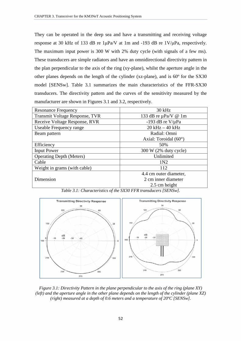
CHAPTER 3. Transceiver for the KM3NeT Acoustic Positioning System
52
They can be operated in the deep sea and have a transmitting and receiving voltage
response at 30 kHz of 133 dB re 1µPa/V at 1m and -193 dB re 1V/µPa, respectively.
The maximum input power is 300 W with 2% duty cycle (with signals of a few ms).
These transducers are simple radiators and have an omnidirectional directivity pattern in
the plan perpendicular to the axis of the ring (xy-plane), whilst the aperture angle in the
other planes depends on the length of the cylinder (xz-plane), and is 60º for the SX30
model [SENSw]. Table 3.1 summarizes the main characteristics of the FFR-SX30
transducers. The directivity pattern and the curves of the sensitivity measured by the
manufacturer are shown in Figures 3.1 and 3.2, respectively.
Resonance Frequency 30 kHz Transmit Voltage Response, TVR 133 dB re µPa/V @ 1m Receive Voltage Response, RVR -193 dB re V/µPa Useable Frequency range 20 kHz – 40 kHz Beam pattern Radial: Omni
Axial: Toroidal (60°) Efficiency 50% Input Power 300 W (2% duty cycle) Operating Depth (Meters) Unlimited Cable 1N2 Weight in grams (with cable) 112
Dimension 4.4 cm outer diameter, 2 cm inner diameter
2.5 cm height Table 3.1: Characteristics of the SX30 FFR transducers [SENSw].
Figure 3.1: Directivity Pattern in the plane perpendicular to the axis of the ring (plane XY) (left) and the aperture angle in the other plane depends on the length of the cylinder (plane XZ)
(right) measured at a depth of 0.6 meters and a temperature of 20ºC [SENSw].
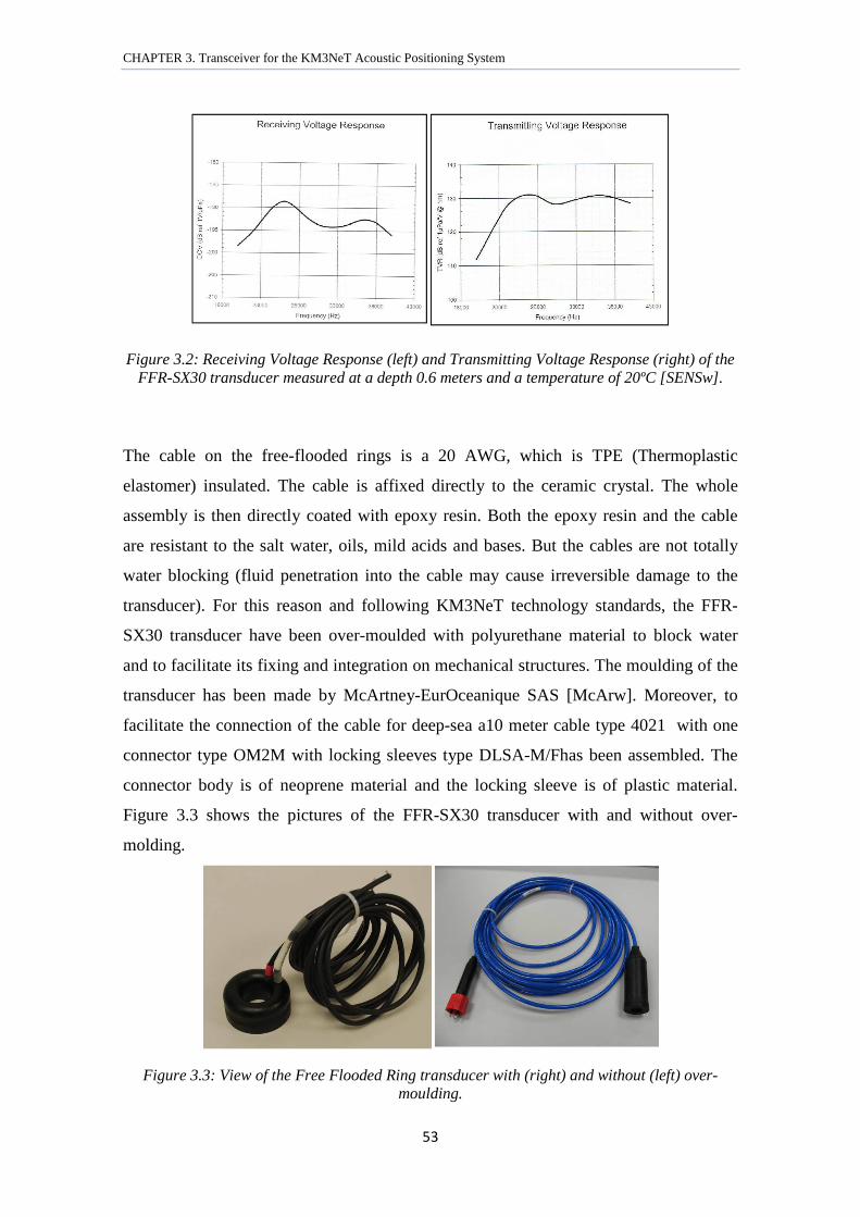
CHAPTER 3. Transceiver for the KM3NeT Acoustic Positioning System
53
Figure 3.2: Receiving Voltage Response (left) and Transmitting Voltage Response (right) of the FFR-SX30 transducer measured at a depth 0.6 meters and a temperature of 20ºC [SENSw].
The cable on the free-flooded rings is a 20 AWG, which is TPE (Thermoplastic
elastomer) insulated. The cable is affixed directly to the ceramic crystal. The whole
assembly is then directly coated with epoxy resin. Both the epoxy resin and the cable
are resistant to the salt water, oils, mild acids and bases. But the cables are not totally
water blocking (fluid penetration into the cable may cause irreversible damage to the
transducer). For this reason and following KM3NeT technology standards, the FFR-
SX30 transducer have been over-moulded with polyurethane material to block water
and to facilitate its fixing and integration on mechanical structures. The moulding of the
transducer has been made by McArtney-EurOceanique SAS [McArw]. Moreover, to
facilitate the connection of the cable for deep-sea a10 meter cable type 4021 with one
connector type OM2M with locking sleeves type DLSA-M/Fhas been assembled. The
connector body is of neoprene material and the locking sleeve is of plastic material.
Figure 3.3 shows the pictures of the FFR-SX30 transducer with and without over-
molding.
Figure 3.3: View of the Free Flooded Ring transducer with (right) and without (left) over-moulding.
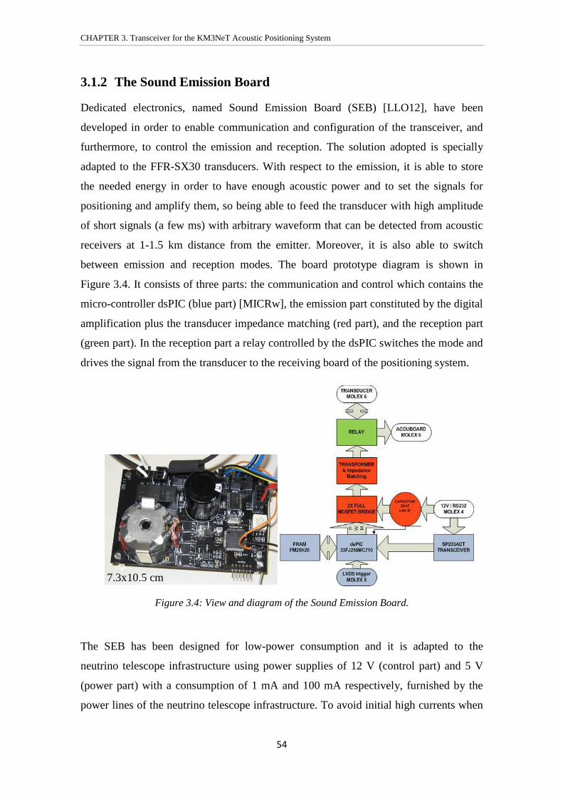
CHAPTER 3. Transceiver for the KM3NeT Acoustic Positioning System
54
3.1.2 The Sound Emission Board
Dedicated electronics, named Sound Emission Board (SEB) [LLO12], have been
developed in order to enable communication and configuration of the transceiver, and
furthermore, to control the emission and reception. The solution adopted is specially
adapted to the FFR-SX30 transducers. With respect to the emission, it is able to store
the needed energy in order to have enough acoustic power and to set the signals for
positioning and amplify them, so being able to feed the transducer with high amplitude
of short signals (a few ms) with arbitrary waveform that can be detected from acoustic
receivers at 1-1.5 km distance from the emitter. Moreover, it is also able to switch
between emission and reception modes. The board prototype diagram is shown in
Figure 3.4. It consists of three parts: the communication and control which contains the
micro-controller dsPIC (blue part) [MICRw], the emission part constituted by the digital
amplification plus the transducer impedance matching (red part), and the reception part
(green part). In the reception part a relay controlled by the dsPIC switches the mode and
drives the signal from the transducer to the receiving board of the positioning system.
Figure 3.4: View and diagram of the Sound Emission Board.
The SEB has been designed for low-power consumption and it is adapted to the
neutrino telescope infrastructure using power supplies of 12 V (control part) and 5 V
(power part) with a consumption of 1 mA and 100 mA respectively, furnished by the
power lines of the neutrino telescope infrastructure. To avoid initial high currents when
7.3x10.5 cm
CHAPTER 3. Transceiver for the KM3NeT Acoustic Positioning System
55
the capacitor starts to charge, there is a current limit of 15 mA. Few seconds later the
current stabilizes at 1 mA. As the instantaneous power available through the telescope
12 V DC distribution system is less than that needed to excite the transducer to cover
long distances, it has been necessary to implement an energy storage block. For this
reason, a capacitor of 22 mF @ 16 V from Panasonic with a very low equivalent series
resistance has been selected. It is able to charge and store the energy needed for the
emission. This solution allows for fast charging, and correspondingly short time delays
between successive emissions (the usual mode of operation is a high-power emission of
a few ms duration every few seconds). The charge of this capacitor is monitored using
the input of the ADC of the micro-controller. Moreover, the output of the micro-
controller is connected through 2x Full MOSFET Driver and a MOSFET full bridge
constituting the power amplifier. The main characteristics for the MOSFETs are the low
Ron (transistor ON resistance) of 11 mΩ, the fast switching (13 ns rise and 4.7 ns fall)
and low gate charge (QG =7.2 nC). Other important characteristics are the high drain
current (Id = 200 A, 0.1 ms signal) and the maximum drain to source voltage (20 V).
The latter is successively connected to the transformer with a frequency and duty cycle
programmed through the micro-controller which also plays the main role of impedance
matching for the transducer. The transformer is able to increase the voltage of the input
signal to an output signal from ~35 Vpp to ~400 Vpp depending on the input values.
Besides, concerning the reception part of the board, it also has the possibility to directly
apply an anti-aliasing filter and return the signal to an ADC of the microcontroller. This
functionality may be very interesting not only in the context of neutrino telescopes, but
also to have the receiver implemented in different underwater applications, such as
affordable sonar systems or echo-sounds.
The micro-controller drives the power amplifier and has two inputs, one for the low
bitrate communication port and one for the trigger signal. Moreover, it contains the
program for the emission of the signals. The signal modulation is done with Pulse-
Width Modulation (PWM) technique which permits the emission of arbitrary intense
short signals [BAR01]. The PWM carry frequency of the emission signal is 400 kHz
and has been tested up to 1.25MHz. The basic idea of this technique is to modulate the
signal digitally at a higher frequency using different width of pulses and the lower
frequency signal is recovered using a low-pass filter (it will be described in the next
section). In addition, it will have an increase in the amplitude of the signal using a full
CHAPTER 3. Transceiver for the KM3NeT Acoustic Positioning System
56
H-Bridge. The communication of the board with the control PC for its configuration is
established through the standard RS232 protocol using an SP233 adapter in the board.
In order to provide a very good timing synchronization the emission is triggered using a
LVDS signal. The delay between the arrived trigger and the emission time depends
slightly on the emitted signals, but the differences between the different signals are
small, about 100 ns.
In summary, the board, designed for an easy integration into a neutrino telescope
infrastructures, can be configured from shore and can emit arbitrary intense short
signals, or act as receiver with very good timing precision (the measured latency is 7 µs
with a stability better than 1 µs), as shown in the KM3NeT APS joint tests [SIM12].
3.1.2.1 Microcontroller and Signal generator block
A microcontroller is composed of a single integrated circuit containing a processor core,
memory, and programmable input/output peripherals. For the signal generator the
Microchip “Motor Control” function inside most of the dsPic microcontroller series has
been chosen. PIC is a family of modified microcontrollers and is used in industrial
developers and hobbyists due to their low cost and wide availability. The dsPic selected
is the dsPic33FJ256MC710 at 16 bit [MICRw]. This microcontroller has 40 MIPS of
processing power for signal processing specific instructions, enough FLASH and RAM
memories for our purposes and a 10 bits @1MSps ADC converter. The “Motor
Control” function is basically a digital counter that works with the main frequency of
the microcontroller (40 MHz). This device has all the necessary components to work
with full MOSFET bridges (symmetric outputs, dead time generators, etc.), and for this
reason matches perfectly for our purposes. Having chosen the full bridge power
amplifier, it must be fed with square signals. This is not a problem if we want to send
square signals like a MLS (Maximum Length Sequence) signal, which is a very useful
signal extensively used in electro-acoustic measurements. The main characteristics of
this signal are the flat spectrum and the non-correlation with any other signal. It can be
used to obtain the impulse response of the entire system and for time of flight
measurements. Moreover, if we wish to send standard sinusoidal or arbitrary signals we
can take advantage of the fact that the transducer and the transformer are good band
pass filters in our band of interest: we can emit a square signal in the band and all the

CHAPTER 3. Transceiver for the KM3NeT Acoustic Positioning System
57
highest frequencies that are out of the working band will be removed. Therefore, we can
also use square signals and obtain sinusoidal signals in the emission, although the best
technique—should we wish to send arbitrary signals by generating squared signals—is
using PWM (Pulse Width Modulation) with a modulation frequency outside the main
band. To implement PWM we must vary the width of the square signal in direct relation
to the voltage of the desired signal (0–100% Pulse width). The classic way to do this is
to compare the desired signal with a triangular or saw tooth signal in order to obtain a
square signal at the output of the comparator. After the amplification, the desired signal
is integrated (filtered by the transformer and the transducer) and the median value of the
square signal is obtained. This median value is the desired signal. In particular, in order
to generate the signal two of the function modes of the motor control are used. The first
is the “free run” mode; in this mode we can obtain a pulse with modulation similar to
the classic one that compares the modulation signal with a saw tooth. Using this mode
when the counter arrives to the PxTPER1 (maximum) value it is reset and starts again
from zero. The device has also other comparators in order to establish the width of the
pulse. The second mode is the “up/down” mode. The only difference between this and
the previous mode is that when the counter arrives to PxTPER it starts counting down
instead of resetting. This mode is similar to the classic PWM modulation that compares
the signal with a triangular wave. With this mode we obtain a more symmetric square
signal with fewer harmonics [LLO12].
3.1.2.2 The firmware
Different firmware versions have been developed in order to adapt the SEB to the
communication prerequisites of the different test installations at the ANTARES and
NEMO neutrino telescope sites (in ANTARES: with MODBUS2 over RS485; in
NEMO: console over RS232). In Figure 3.5 the basic working process is described. The
basic firmware has three main parts. The first is the processing of commands that arrive
at the low bitrate communication port: these commands usually are used to configure
the board or define the signal to be emitted. The second block is in the main part of the
program and is aware of the trigger port in order to start the emission when a trigger
1 PxTPER is the PWM time base period register. It sets the maximum value of the counter.
2 MODBUS is a communication protocol used in industrial environments.

CHAPTER 3. Transceiver for the KM3NeT Acoustic Positioning System
58
signal arrives. The third block is an interrupt code that works when the “Motor Control”
counter arrives to the PxTPER register. This code changes the registers of the “Motor
Control” device in order to obtain the next cycle of the desired square signal (frequency,
pulse width, etc.) [LLO12].
Figure 3.5: Diagram of the firmware working process.
3.2 Sensitivity tests of the FFR-SX30
With the objective to study the possibility of using the FFR transducers as emitters and
receiver in the APS of KM3NeT neutrino telescope several studies have been done.
The first tests were done in the laboratory of Gandia in order to characterize the
transducers in terms of the transmitting and receiving voltage responses (TVR, RVR) as
a function of the frequency and as a function of the angle (directivity pattern). The tests
have been performed in a fresh-water tank with dimension of 87.5 x 113 x 56.5 cm3. For
the tests omnidirectional calibrated transducers, model ITC-1042 [ITCw] (with
transmitting voltage response 148 dB ref. 1µPa/V @ 1 m) and RESON-TC4014
[RESOw] (with receiving voltage response -186 dB ± 3 dB re 1V/µPa) have been used
as reference emitter and receiver, respectively. The FFR-SX30 transducers were used as
emitters and receivers in order to calculate their TVR and RVR, respectively. Figure 3.6
shows the used position for the study of the sensitivity of the FFR-SX30 transducers
which will be named position 1 and 2. In the position 1 the sensitivity is omnidirectional
for the horizontal plane, whereas in the position 2 the sensitivity changes as function of
the angle. The FFR-SX30 transducer was placed at 10 cm from the reference
transducers with the aim to study their sensitivity as a function of the frequency and as a
function angle (directivity pattern) in the position 1 and position 2 (Fig.3.7-3.8).

CHAPTER 3. Transceiver for the KM3NeT Acoustic Positioning System
59
Besides, different tone bursts signals with 5 Vp and 10 Vp of amplitude and 5 cycle
length in the frequency range 18-42 kHz were generated through a NI PCI-5412 board
[NATIw] controlled with a control PC. A LabVIEW program was used for the
emission, reception and recording of the data. The received signals were amplified from
a RESON CCA100 (1nF = Input Capacitance, 10kΩ = Input Resistance, X dB = output
gain used) and RESON EC6073 preamplifier for the FFR-SX30 and Reson-TC4014
receiver hydrophones respectively. A positioning motor made by ISEL automation and
PI micos, Germany [ISELw, MICOw], have been used to position the hydrophone in
the tank. It is able to move in the three dimension x, y and z and has an accuracy of
0.01mm. The signal length was chosen according to the dimensions of the tank to avoid
the interference of the reflected signals from the walls and water surface with the direct
signal.
Figure 3.6: Scheme of the used position (orientation) for the measurements of sensitivity for the FFR-SX30 transducers.
Figure 3.7: Configuration used to calculate RVR of the FFR-SX30 as a function of the frequency and as a function of the angle (directivity pattern) in position 1 (left) and position 2
(right).
Receivers
10 cm
Emitter
-90º
+90º Emitter
Receivers
Direction of
emission or
reception
Position 1
Direction of
emission or
reception
Position 2
CHAPTER 3. Transceiver for the KM3NeT Acoustic Positioning System
60
Figure 3.8: Configuration used to calculate TVR of the FFR-SX30 as a function of the frequency and as a function of the angle (directivity pattern) in the position 1 (left) and position
2 (right).
Furthermore measurements in the anechoic chamber of the Campus de Gandia were
done in order to acquire the electronic noise of the FFR-SX30 hydrophones as receivers.
Figure 3.9 shows the power spectrum density of some FFR hydrophones. The level of
the noise is below -120 dB re V2/Hz (~ ≤Sea State3 1, that is of the sea ambient noise in
the state 1).
Figure 3.9: Power density spectrum of some FFR-SX30 hydrophone. The level noise is below -120 dB re V2/Hz (~ ≤Sea State 1).
3 The Sea State is the general condition of the free surface on a large body of water and depends of wind speed and wave height. Sea Sate 0 is the calm sea.
0 1 2 3 4 5 6 7 8 9 10
x 104
-160
-150
-140
-130
-120
-110
-100
-90
-80
Frequency [Hz]
Am
plitu
de (d
B re
f 1V2
/Hz)
FFR-530FFR-04FFR-03
Emitter
Receiver
-90º
+90º
Emitter
10 cm
Receiver

CHAPTER 3. Transceiver for the KM3NeT Acoustic Positioning System
61
The equation used to calculate the receiving voltage response is:
= + 20 · − dB;[dBre1V/µPa]
(3.1)
where:
is the sensitivity in dB of the FFR-SX30 (unknown).
is the sensitivity in dB of the calibrated Reson hydrophone (known) .
.. is the amplitude of the signal in V received by FFR-SX30 hydrophone.
.. is the amplitude of the signal in V received by calibrated Reson hydrophone.
are the different gains selected in the preamplifier connected to the FFR-SX30
receiver hydrophones.
The equation used to calculate the Transmitting Voltage Response of the FFR
hydrophones is the following:
/ = 20 · 0112@14 · 105 · 612/12
.7. 8 ; [9:1612/.]
(3.2)
where:
/ is the Transmitting Voltage Response in dB of the transducer (unknown).
.7. is the value of the amplitude of the emitted signal by the FFR-SX30 transducer.
112@14 is the pressure measured at the distance of 1 m by the emitter transducer.
It is calculated by the following equation:
112@14 = ;<=>=?@=<;AB?C=D<;/EF GHH [Pa]
where .IJ7KI. is the value of the amplitude of the received signal in V by the
calibrated Reson TC4014 hydrophone when the FFR-SX30 transducer emits, L7FI./
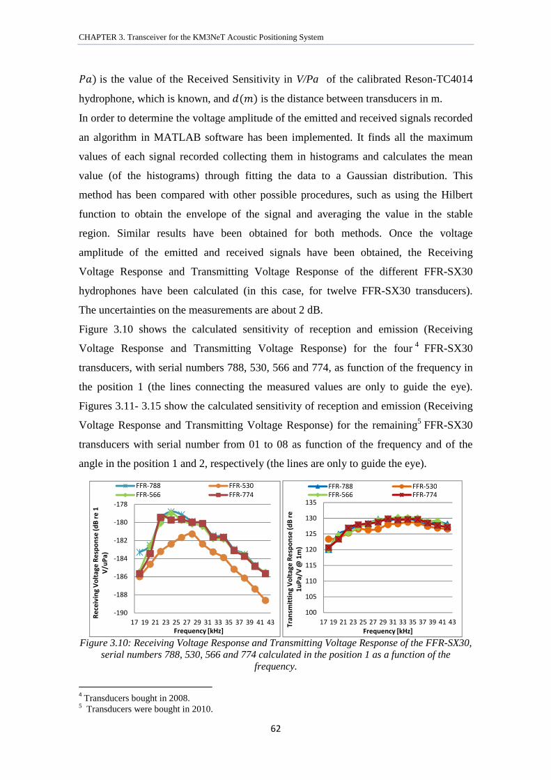
CHAPTER 3. Transceiver for the KM3NeT Acoustic Positioning System
62
12 is the value of the Received Sensitivity in V/Pa of the calibrated Reson-TC4014
hydrophone, which is known, and 4 is the distance between transducers in m.
In order to determine the voltage amplitude of the emitted and received signals recorded
an algorithm in MATLAB software has been implemented. It finds all the maximum
values of each signal recorded collecting them in histograms and calculates the mean
value (of the histograms) through fitting the data to a Gaussian distribution. This
method has been compared with other possible procedures, such as using the Hilbert
function to obtain the envelope of the signal and averaging the value in the stable
region. Similar results have been obtained for both methods. Once the voltage
amplitude of the emitted and received signals have been obtained, the Receiving
Voltage Response and Transmitting Voltage Response of the different FFR-SX30
hydrophones have been calculated (in this case, for twelve FFR-SX30 transducers).
The uncertainties on the measurements are about 2 dB.
Figure 3.10 shows the calculated sensitivity of reception and emission (Receiving
Voltage Response and Transmitting Voltage Response) for the four4 FFR-SX30
transducers, with serial numbers 788, 530, 566 and 774, as function of the frequency in
the position 1 (the lines connecting the measured values are only to guide the eye).
Figures 3.11- 3.15 show the calculated sensitivity of reception and emission (Receiving
Voltage Response and Transmitting Voltage Response) for the remaining5 FFR-SX30
transducers with serial number from 01 to 08 as function of the frequency and of the
angle in the position 1 and 2, respectively (the lines are only to guide the eye).
Figure 3.10: Receiving Voltage Response and Transmitting Voltage Response of the FFR-SX30, serial numbers 788, 530, 566 and 774 calculated in the position 1 as a function of the
frequency.
4 Transducers bought in 2008.
5 Transducers were bought in 2010.
-190
-188
-186
-184
-182
-180
-178
17 19 21 23 25 27 29 31 33 35 37 39 41 43
Re
ceiv
ing
Vo
lta
ge
Re
spo
nse
(d
B r
e 1
V/u
Pa
)
Frequency [kHz]
FFR-788 FFR-530
FFR-566 FFR-774
100
105
110
115
120
125
130
135
17 19 21 23 25 27 29 31 33 35 37 39 41 43Tra
nsm
itti
ng
Vo
lta
ge
Re
spo
nse
(d
B r
e
1u
Pa
/V @
1m
)
Frequency [kHz]
FFR-788 FFR-530
FFR-566 FFR-774
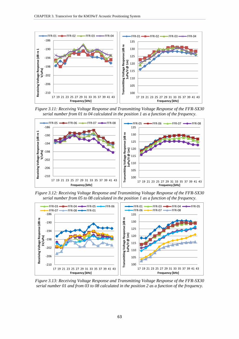
CHAPTER 3. Transceiver for the KM3NeT Acoustic Positioning System
63
Figure 3.11: Receiving Voltage Response and Transmitting Voltage Response of the FFR-SX30 serial number from 01 to 04 calculated in the position 1 as a function of the frequency.
Figure 3.12: Receiving Voltage Response and Transmitting Voltage Response of the FFR-SX30 serial number from 05 to 08 calculated in the position 1 as a function of the frequency.
Figure 3.13: Receiving Voltage Response and Transmitting Voltage Response of the FFR-SX30 serial number 01 and from 03 to 08 calculated in the position 2 as a function of the frequency.
-210
-206
-202
-198
-194
-190
-186
17 19 21 23 25 27 29 31 33 35 37 39 41 43Re
ceiv
ing
Vo
lta
ge
Re
spo
nse
(d
B r
e 1
V/u
Pa
)
Frequency [kHz]
FFR-01 FFR-02 FFR-03 FFR-04
100
105
110
115
120
125
130
135
17 19 21 23 25 27 29 31 33 35 37 39 41 43
Tra
nsm
itti
ng
Vo
lta
ge
Re
spo
nse
(d
B r
e
1u
Pa
/V @
1m
)
Frequency [kHz]
FFR-01 FFR-02 FFR-03 FFR-04
-210
-206
-202
-198
-194
-190
-186
17 19 21 23 25 27 29 31 33 35 37 39 41 43
Re
ceiv
ing
Vo
lta
ge
Re
spo
nse
(d
B r
e 1
V/u
Pa
)
Frequency [kHz]
FFR-05 FFR-06 FFR-07 FFR-08
100
105
110
115
120
125
130
135
17 19 21 23 25 27 29 31 33 35 37 39 41 43Tra
nsm
itti
ng
Vo
lta
ge
Re
spo
nse
(d
B r
e
1u
Pa
/V @
1m
)
Frequency [kHz]
FFR-05 FFR-06 FFR-07 FFR-08
-210
-206
-202
-198
-194
-190
-186
17 19 21 23 25 27 29 31 33 35 37 39 41 43
Re
ceiv
ing
Vo
lta
ge
Re
spo
nse
(d
B r
e
1V
/uP
a)
Frequency [kHz]
FFR-03 FFR-04 FFR-05 FFR-06
FFR-07 FFR-08 FFR-01
100
105
110
115
120
125
130
135
17 19 21 23 25 27 29 31 33 35 37 39 41 43
Tra
nsm
itti
ng
Vo
lta
ge
Re
spo
nse
(d
B r
e
1u
Pa
/V @
1m
)
Frequency [kHz]
FFR-01 FFR-03 FFR-04 FFR-05
FFR-06 FFR-07 FFR-08
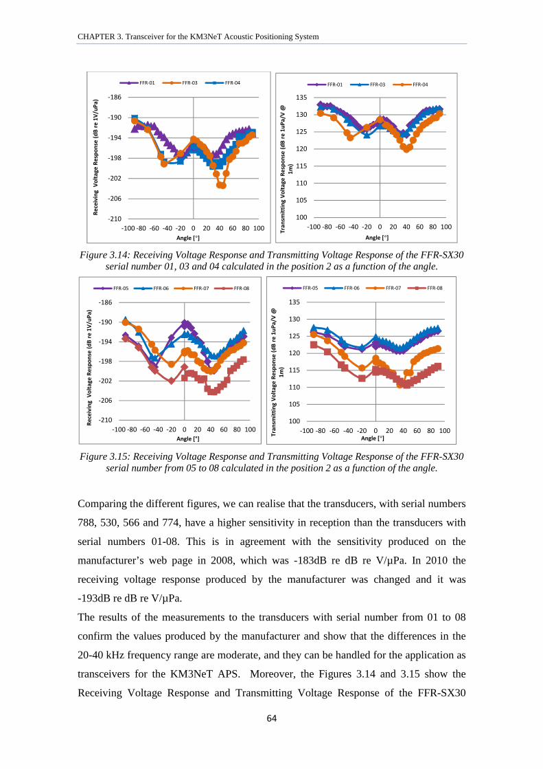
CHAPTER 3. Transceiver for the KM3NeT Acoustic Positioning System
64
Figure 3.14: Receiving Voltage Response and Transmitting Voltage Response of the FFR-SX30 serial number 01, 03 and 04 calculated in the position 2 as a function of the angle.
Figure 3.15: Receiving Voltage Response and Transmitting Voltage Response of the FFR-SX30 serial number from 05 to 08 calculated in the position 2 as a function of the angle.
Comparing the different figures, we can realise that the transducers, with serial numbers
788, 530, 566 and 774, have a higher sensitivity in reception than the transducers with
serial numbers 01-08. This is in agreement with the sensitivity produced on the
manufacturer’s web page in 2008, which was -183dB re dB re V/µPa. In 2010 the
receiving voltage response produced by the manufacturer was changed and it was
-193dB re dB re V/µPa.
The results of the measurements to the transducers with serial number from 01 to 08
confirm the values produced by the manufacturer and show that the differences in the
20-40 kHz frequency range are moderate, and they can be handled for the application as
transceivers for the KM3NeT APS. Moreover, the Figures 3.14 and 3.15 show the
Receiving Voltage Response and Transmitting Voltage Response of the FFR-SX30
-210
-206
-202
-198
-194
-190
-186
-100 -80 -60 -40 -20 0 20 40 60 80 100
Re
ceiv
ing
V
olt
ag
e R
esp
on
se (
dB
re
1V
/uP
a)
Angle [°]
FFR-01 FFR-03 FFR-04
100
105
110
115
120
125
130
135
-100 -80 -60 -40 -20 0 20 40 60 80 100
Tra
nsm
itti
ng
Vo
lta
ge
Re
spo
nse
(d
B r
e 1
uP
a/V
@
1m
)
Angle [°]
FFR-01 FFR-03 FFR-04
-210
-206
-202
-198
-194
-190
-186
-100 -80 -60 -40 -20 0 20 40 60 80 100
Re
ceiv
ing
V
olt
ag
e R
esp
on
se (
dB
re
1V
/uP
a)
Angle [°]
FFR-05 FFR-06 FFR-07 FFR-08
100
105
110
115
120
125
130
135
-100 -80 -60 -40 -20 0 20 40 60 80 100
Tra
nsm
itti
ng
Vo
lta
ge
Re
spo
nse
(d
B r
e 1
uP
a/V
@
1m
)
Angle [°]
FFR-05 FFR-06 FFR-07 FFR-08
CHAPTER 3. Transceiver for the KM3NeT Acoustic Positioning System
65
transducers as a function of the angle using a 30 kHz tone burst signal (measured in the
position 2 where 0º corresponds to the direction opposite to the cables). As expected, a
minimum of sensitivity appears at about 30º due to the shape of the transducer. These
latter variations of sensitivity are about 5 dB (almost 50%) to each one transducer,
which is a noticeable value, but, again these variations in sensitivity can be handled
without major problems for the use as transceiver for the KM3NeT APS application. In
case the FFR-SX30 will be used as receiver hydrophones for the KM3NeT APS, a good
parameterisation of the sensitivity as a function of the frequency and angle for each
transducer will be needed, especially for the potential use of these hydrophones for
deep-sea acoustic monitoring studies or for the acoustic detection of Ultra-High-Energy
neutrinos. For this application, it would be good to have precise measurements of the
sensitivities at larger distances between both transducers, and some work is going on
within the research group in that respect.
3.3 Pressure tests
One of the most important requirements for the KM3NeT detector is the possibility of
using the selected transducers under high pressure [ARD10]. For this reason, a
measurement campaign using a large hyperbaric tank at IFREMER (Institut Francais de
Recherche pour L’exploitation de la Mer) research facilities at Plouzane (near Brest,
France) was performed in 2009. The aim of these measurements was to study the
behaviour of four FFR-SX30 transducers under different values of pressure, in the
frequency range of interest 21 kHz – 42 kHz, recording the emitted and received signals
and then, observing the relative acoustic power variations. Two hydrophones and a
sound velocimeter used in the ANTARES submarine neutrino detector were also tested
(the study of these devices has not been part of this thesis). Figure 3.16 shows the fresh-
water hyperbaric tank used to simulate the pressure in large water depth and a table with
its main characteristics.
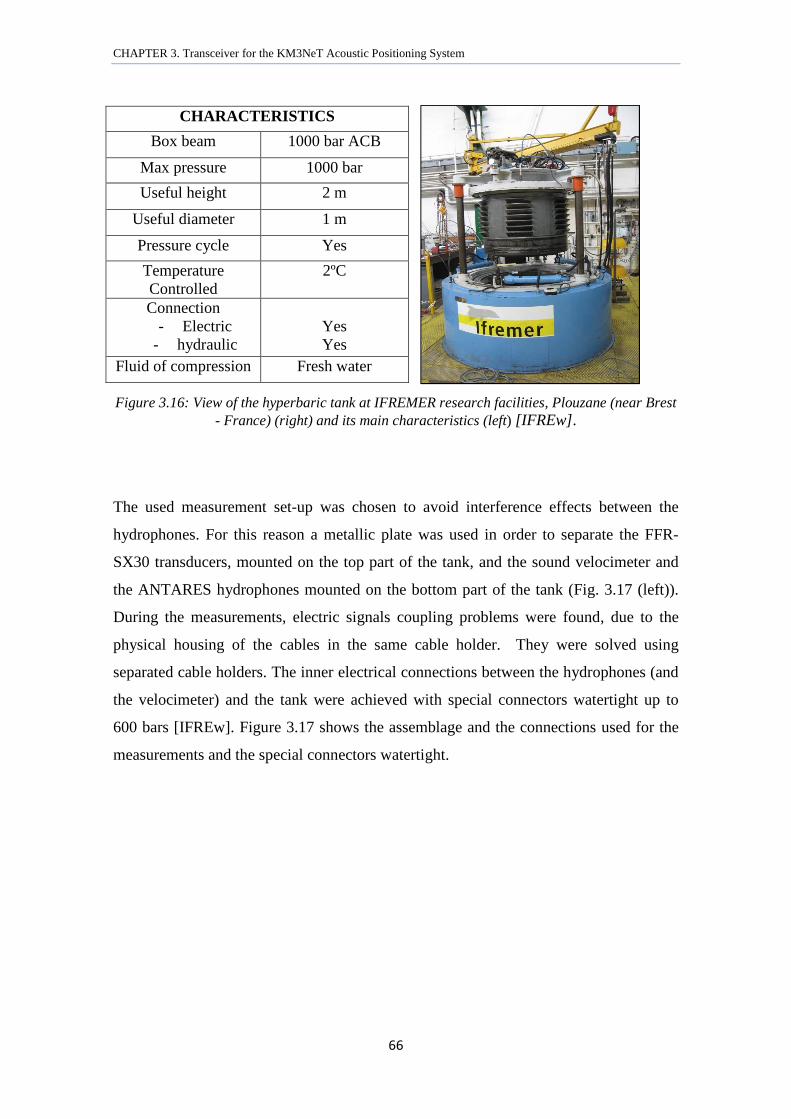
CHAPTER 3. Transceiver for the KM3NeT Acoustic Positioning System
66
Figure 3.16: View of the hyperbaric tank at IFREMER research facilities, Plouzane (near Brest - France) (right) and its main characteristics (left) [IFREw].
The used measurement set-up was chosen to avoid interference effects between the
hydrophones. For this reason a metallic plate was used in order to separate the FFR-
SX30 transducers, mounted on the top part of the tank, and the sound velocimeter and
the ANTARES hydrophones mounted on the bottom part of the tank (Fig. 3.17 (left)).
During the measurements, electric signals coupling problems were found, due to the
physical housing of the cables in the same cable holder. They were solved using
separated cable holders. The inner electrical connections between the hydrophones (and
the velocimeter) and the tank were achieved with special connectors watertight up to
600 bars [IFREw]. Figure 3.17 shows the assemblage and the connections used for the
measurements and the special connectors watertight.
CHARACTERISTICS
Box beam 1000 bar ACB
Max pressure 1000 bar
Useful height 2 m
Useful diameter 1 m
Pressure cycle Yes
Temperature Controlled
2ºC
Connection - Electric
- hydraulic
Yes Yes
Fluid of compression Fresh water

CHAPTER 3. Transceiver for the KM3NeT Acoustic Positioning System
67
Figure 3.17: Views of the assemblage and the electrical connections used for the measurement (left and top right) and of the special connectors watertight up to 600 bars (bottom right).
The pressure dependence on the transceivers in both conditions of rising and decreasing
pressures in the range from 1 to 440 bars was investigated. For each pressure value,
different tone bursts signals with 10 Vp of amplitude and 10 cycle length in the
frequency range 18-42 kHz were emitted. The latter were generated through a signal
generator and sent to a pair of emitter-receiver FFR-SX30 transducer. Successively, the
received signals were amplified through a CCA100 amplifier RESON (1n = Input
Capacitance, 10k = Input Resistance, 12 = dB output gain) and recorded with a NI USB-
5132 board by National Instrument [NATIw] managed with a control PC through USB
port. The signals are recorded as a text file containing a matrix which columns hold the
time and the emitted and received signal wave form.
In order to test the transducers at high pressure for a long time, the transducers and the
sound velocimeter were left at the pressure of 440 bars for all the night.
In Figure 3.18 an example of the emitted and received signal at 30 kHz and 440 bars of
pressure for the pair of emitter-receiver FFR-SX30 transducer are shown.
FFR SX30
774-788-566
FFR SX30
530
Velocimeter ANTARES
hydrophone

CHAPTER 3. Transceiver for the KM3NeT Acoustic Positioning System
68
Figure 3.18: Emitted (blue line) and received signal (red line) to the pair of emitter-receiver
FFR-SX30 530 and FFR-SX30 788 at 440 bar of pressure.
In order to calculate the acoustic power variation as a function of the pressure only the
recorded files in the conditions of decreasing pressures (440, 300, 200, 50, 1 bar) was
analyzed. A problem was found during the measurements in the conditions of rising
pressures (at the pressure of 1, 50, 200, 300 bar), some hydrophones did not work due to
bad connections and the data could not be used in the analysis.
The variation of the amplitude in the frequency spectrum at different pressure and
frequency was analyzed, considering only the received direct signal without taking into
account the reflections. In this way, for each frequency and pressure, the maximum
amplitude of the Power Spectral Density (PSD) using Welch's method of MATLAB
was calculated. Figure 3.19 shows an example of the results obtained from these
measurements for the acoustic transmission between two FFR-SX30 transducers as a
function of the frequency and pressure. The uncertainties of the measurement are about
1.0 dB. Moreover, only the frequencies range 24-40 kHz is shown due to the bad signal
to noise ratio measured for other frequencies.
0 1 2 3 4 5 6
x 10-4
-10
-8
-6
-4
-2
0
2
4
6
8
10
12
Time [s]
Am
plitu
de [V
]
hydrophone emitter 530 - receiver 788 - 440 bars
emitted signalreceived signal
delay
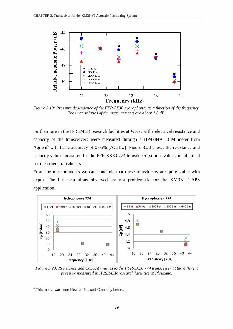
CHAPTER 3. Transceiver for the KM3NeT Acoustic Positioning System
69
Figure 3.19: Pressure dependence of the FFR-SX30 hydrophones as a function of the frequency. The uncertainties of the measurements are about 1.0 dB.
Furthermore in the IFREMER research facilities at Plouzane the electrical resistance and
capacity of the transceivers were measured through a HP4284A LCM meter from
Agilent6 with basic accuracy of 0.05% [AGILw]. Figure 3.20 shows the resistance and
capacity values measured for the FFR-SX30 774 transducer (similar values are obtained
for the others transducers).
From the measurements we can conclude that these transducers are quite stable with
depth. The little variations observed are not problematic for the KM3NeT APS
application.
Figure 3.20: Resistance and Capacity values to the FFR-SX30 774 transceiver at the different pressure measured in IFREMER research facilities at Plouzane.
6 This model was from Hewlett Packard Company before.
0
10
20
30
40
50
60
16 20 24 28 32 36 40 44
Rp
[k
oh
m]
Frequency [kHz]
Hydrophones 774
1 Bar 59 Bar 200 Bar 300 Bar 440 Bar
4
4,2
4,4
4,6
4,8
5
16 20 24 28 32 36 40 44
Cp
[n
F]
Frequency [kHz]
Hydrophones 774
1 Bar 50 Bar 200 Bar 300 Bar 440 Bar

CHAPTER 3. Transceiver for the KM3NeT Acoustic Positioning System
70
3.4 Tests on the Transceiver
The transceiver has been tested in a fresh-water tank in the laboratory, in a pool and in
shallow sea water in order to be integrated in the instrumentation line of the ANTARES
neutrino telescope and in the NEMO Phase II tower for the in situ tests in the deep sea.
For simplicity and due to limitations applying for the integration in both experiments, it
was decided to test the transceiver only as an emitter. The receiver functionality will be
tested in other in situ KM3NeT tests.
To test the system, the transceiver has been used with different emission configurations
in combination with the omnidirectional transducer RESON-TC4014, which was used
as receiver. Different signals have been used (tone bursts, sine sweeps, maximum length
sequence MLS signals, etc.) to study the performance of the transducer in different
situations. In order to study with accuracy the performance of the system the positioning
system mounted on the tank has been used to position the hydrophone in it. It allows the
motion in three dimension x, y and z with an accuracy of 0.01 mm. Figures 3.21 and
3.22 show the configuration of the transceiver (named position 1 and 2, as explained
above) and the set up used for the measurements. In the next section, the activities and
results of these tests are described.
Figure 3.21: Configuration used to test the system as a function of the frequency (position 1, left) and as a function angle (position 2, right).
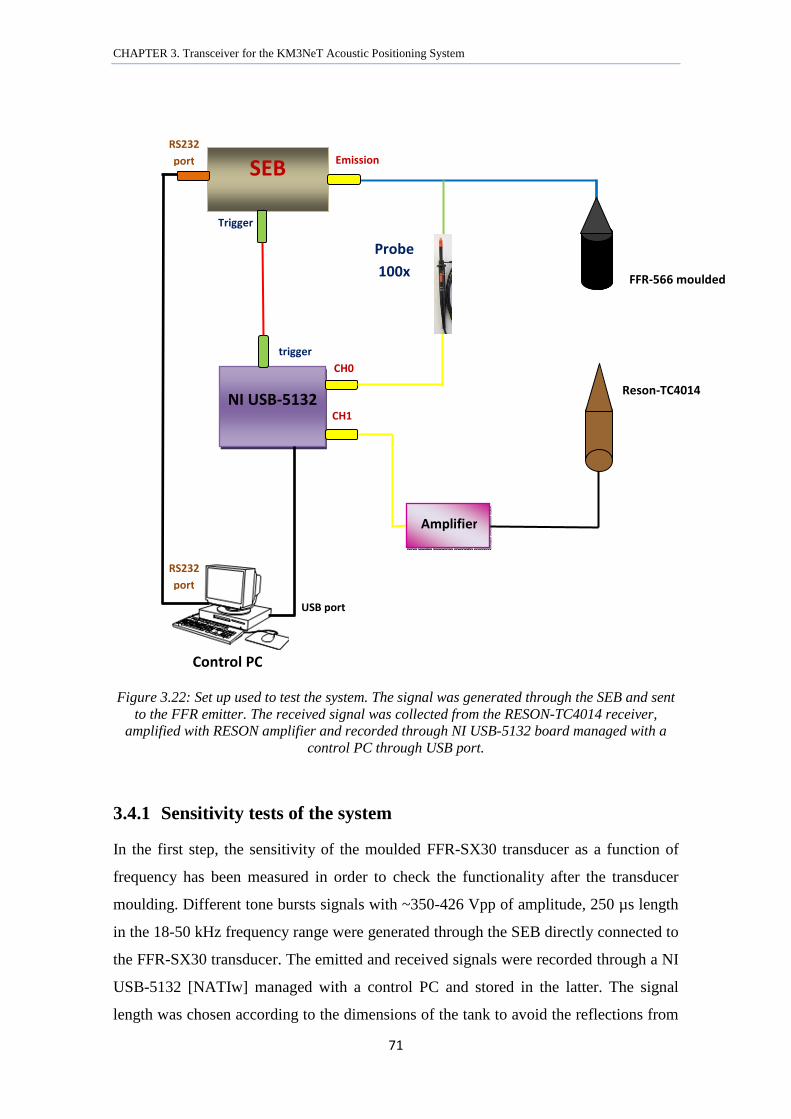
CHAPTER 3. Transceiver for the KM3NeT Acoustic Positioning System
71
Figure 3.22: Set up used to test the system. The signal was generated through the SEB and sent to the FFR emitter. The received signal was collected from the RESON-TC4014 receiver,
amplified with RESON amplifier and recorded through NI USB-5132 board managed with a control PC through USB port.
3.4.1 Sensitivity tests of the system
In the first step, the sensitivity of the moulded FFR-SX30 transducer as a function of
frequency has been measured in order to check the functionality after the transducer
moulding. Different tone bursts signals with ~350-426 Vpp of amplitude, 250 µs length
in the 18-50 kHz frequency range were generated through the SEB directly connected to
the FFR-SX30 transducer. The emitted and received signals were recorded through a NI
USB-5132 [NATIw] managed with a control PC and stored in the latter. The signal
length was chosen according to the dimensions of the tank to avoid the reflections from
SEB
FFR-566 moulded
Control PC
NI USB-5132
CH0
CH1
trigger
Emission
Trigger
Reson-TC4014
Amplifier
Probe
100x
RS232
port
RS232
port
USB port
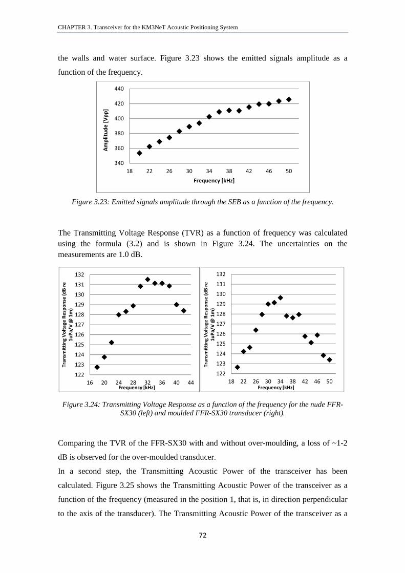
CHAPTER 3. Transceiver for the KM3NeT Acoustic Positioning System
72
the walls and water surface. Figure 3.23 shows the emitted signals amplitude as a
function of the frequency.
Figure 3.23: Emitted signals amplitude through the SEB as a function of the frequency.
The Transmitting Voltage Response (TVR) as a function of frequency was calculated using the formula (3.2) and is shown in Figure 3.24. The uncertainties on the measurements are 1.0 dB.
Figure 3.24: Transmitting Voltage Response as a function of the frequency for the nude FFR-SX30 (left) and moulded FFR-SX30 transducer (right).
Comparing the TVR of the FFR-SX30 with and without over-moulding, a loss of ~1-2
dB is observed for the over-moulded transducer.
In a second step, the Transmitting Acoustic Power of the transceiver has been
calculated. Figure 3.25 shows the Transmitting Acoustic Power of the transceiver as a
function of the frequency (measured in the position 1, that is, in direction perpendicular
to the axis of the transducer). The Transmitting Acoustic Power of the transceiver as a
340
360
380
400
420
440
18 22 26 30 34 38 42 46 50
Am
pli
tud
e [
Vp
p]
Frequency [kHz]
122
123
124
125
126
127
128
129
130
131
132
16 20 24 28 32 36 40 44
Tra
nsm
itti
ng
Vo
lta
ge
Re
spo
nse
(d
B r
e
1u
Pa
/V @
1m
)
Frequency [kHz]
122
123
124
125
126
127
128
129
130
131
132
18 22 26 30 34 38 42 46 50
Tra
nsm
itti
ng
Vo
lta
ge
Re
spo
nse
(d
B r
e
1u
Pa
/V @
1m
)
Frequency [kHz]
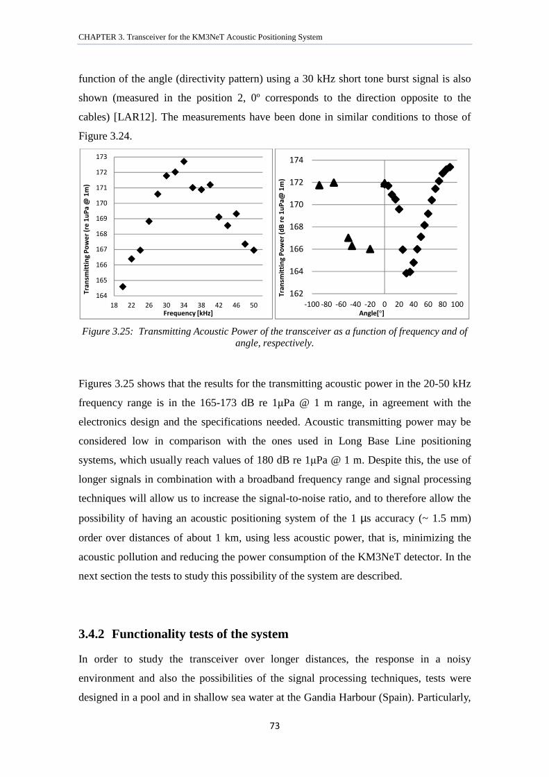
CHAPTER 3. Transceiver for the KM3NeT Acoustic Positioning System
73
function of the angle (directivity pattern) using a 30 kHz short tone burst signal is also
shown (measured in the position 2, 0º corresponds to the direction opposite to the
cables) [LAR12]. The measurements have been done in similar conditions to those of
Figure 3.24.
Figure 3.25: Transmitting Acoustic Power of the transceiver as a function of frequency and of angle, respectively.
Figures 3.25 shows that the results for the transmitting acoustic power in the 20-50 kHz
frequency range is in the 165-173 dB re 1µPa @ 1 m range, in agreement with the
electronics design and the specifications needed. Acoustic transmitting power may be
considered low in comparison with the ones used in Long Base Line positioning
systems, which usually reach values of 180 dB re 1µPa @ 1 m. Despite this, the use of
longer signals in combination with a broadband frequency range and signal processing
techniques will allow us to increase the signal-to-noise ratio, and to therefore allow the
possibility of having an acoustic positioning system of the 1 µs accuracy (~ 1.5 mm)
order over distances of about 1 km, using less acoustic power, that is, minimizing the
acoustic pollution and reducing the power consumption of the KM3NeT detector. In the
next section the tests to study this possibility of the system are described.
3.4.2 Functionality tests of the system
In order to study the transceiver over longer distances, the response in a noisy
environment and also the possibilities of the signal processing techniques, tests were
designed in a pool and in shallow sea water at the Gandia Harbour (Spain). Particularly,
164
165
166
167
168
169
170
171
172
173
18 22 26 30 34 38 42 46 50
Tra
nsm
itti
ng
Po
we
r (r
e 1
uP
a @
1m
)
Frequency [kHz]
162
164
166
168
170
172
174
-100 -80 -60 -40 -20 0 20 40 60 80 100
Tra
nsm
itti
ng
Po
we
r (d
B r
e 1
uP
a@
1m
)
Angle[°]
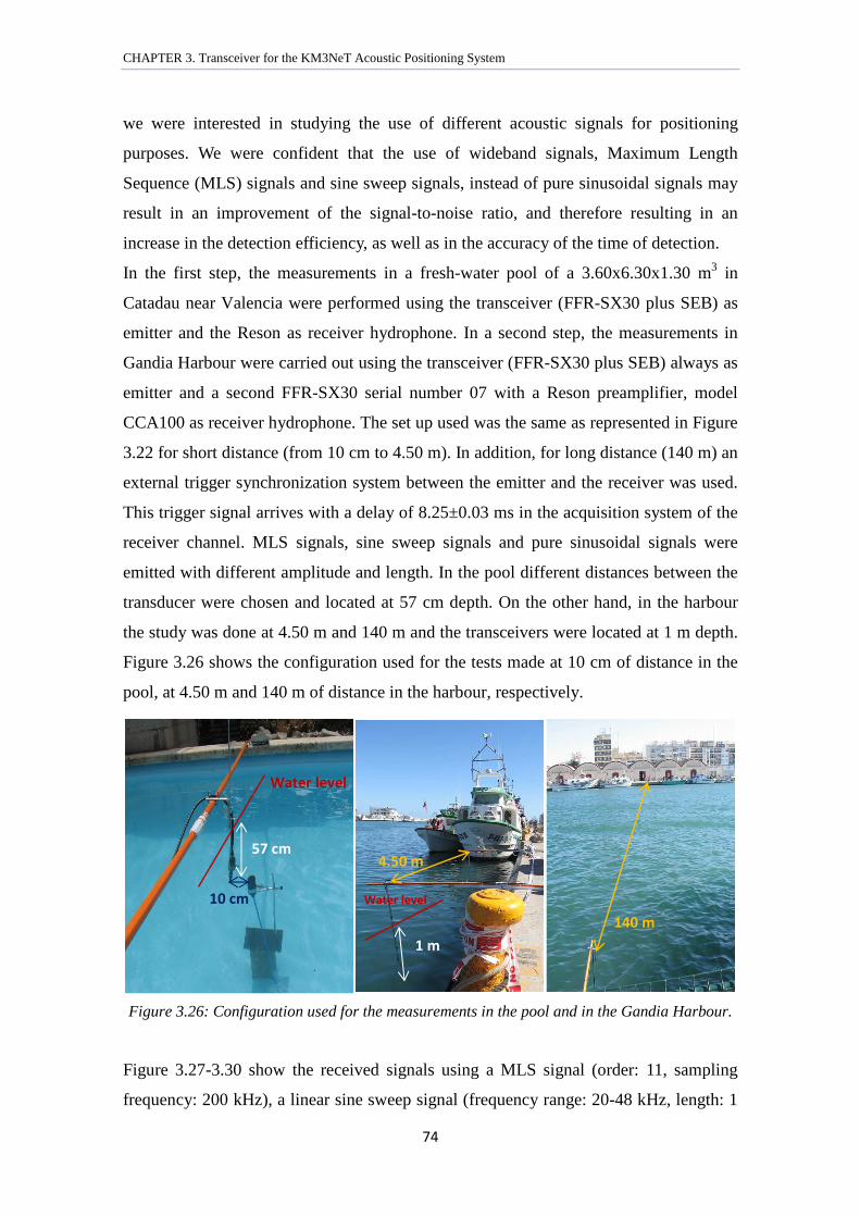
CHAPTER 3. Transceiver for the KM3NeT Acoustic Positioning System
74
we were interested in studying the use of different acoustic signals for positioning
purposes. We were confident that the use of wideband signals, Maximum Length
Sequence (MLS) signals and sine sweep signals, instead of pure sinusoidal signals may
result in an improvement of the signal-to-noise ratio, and therefore resulting in an
increase in the detection efficiency, as well as in the accuracy of the time of detection.
In the first step, the measurements in a fresh-water pool of a 3.60x6.30x1.30 m3 in
Catadau near Valencia were performed using the transceiver (FFR-SX30 plus SEB) as
emitter and the Reson as receiver hydrophone. In a second step, the measurements in
Gandia Harbour were carried out using the transceiver (FFR-SX30 plus SEB) always as
emitter and a second FFR-SX30 serial number 07 with a Reson preamplifier, model
CCA100 as receiver hydrophone. The set up used was the same as represented in Figure
3.22 for short distance (from 10 cm to 4.50 m). In addition, for long distance (140 m) an
external trigger synchronization system between the emitter and the receiver was used.
This trigger signal arrives with a delay of 8.25±0.03 ms in the acquisition system of the
receiver channel. MLS signals, sine sweep signals and pure sinusoidal signals were
emitted with different amplitude and length. In the pool different distances between the
transducer were chosen and located at 57 cm depth. On the other hand, in the harbour
the study was done at 4.50 m and 140 m and the transceivers were located at 1 m depth.
Figure 3.26 shows the configuration used for the tests made at 10 cm of distance in the
pool, at 4.50 m and 140 m of distance in the harbour, respectively.
Figure 3.26: Configuration used for the measurements in the pool and in the Gandia Harbour.
Figure 3.27-3.30 show the received signals using a MLS signal (order: 11, sampling
frequency: 200 kHz), a linear sine sweep signal (frequency range: 20-48 kHz, length: 1
10 cm
57 cm
Water level
4.50 m
140 m
1 m
Water level
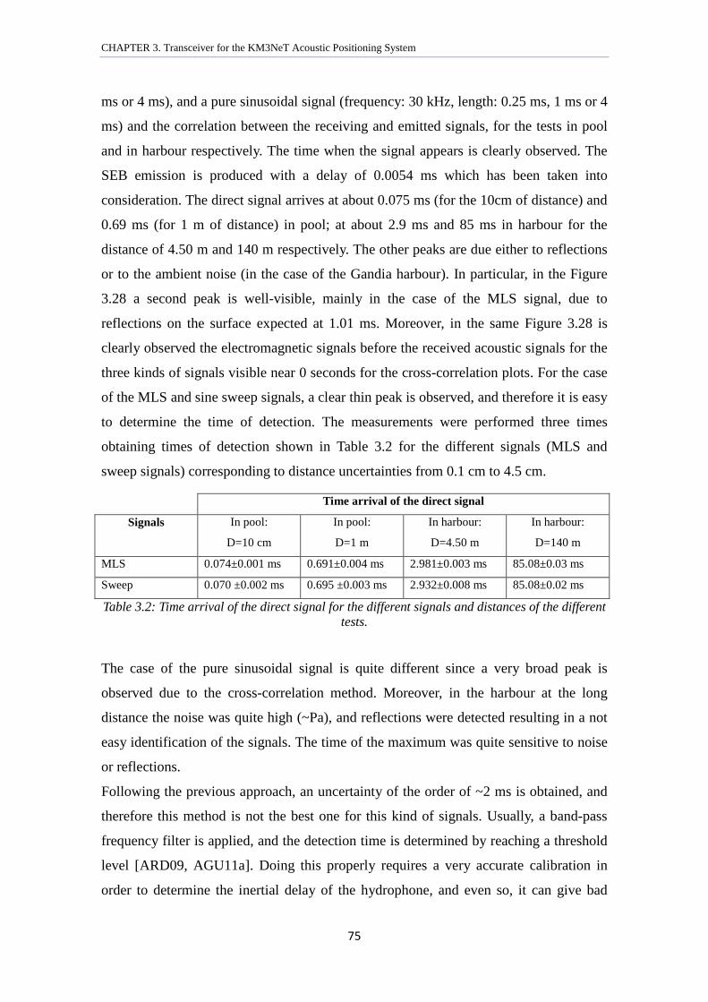
CHAPTER 3. Transceiver for the KM3NeT Acoustic Positioning System
75
ms or 4 ms), and a pure sinusoidal signal (frequency: 30 kHz, length: 0.25 ms, 1 ms or 4
ms) and the correlation between the receiving and emitted signals, for the tests in pool
and in harbour respectively. The time when the signal appears is clearly observed. The
SEB emission is produced with a delay of 0.0054 ms which has been taken into
consideration. The direct signal arrives at about 0.075 ms (for the 10cm of distance) and
0.69 ms (for 1 m of distance) in pool; at about 2.9 ms and 85 ms in harbour for the
distance of 4.50 m and 140 m respectively. The other peaks are due either to reflections
or to the ambient noise (in the case of the Gandia harbour). In particular, in the Figure
3.28 a second peak is well-visible, mainly in the case of the MLS signal, due to
reflections on the surface expected at 1.01 ms. Moreover, in the same Figure 3.28 is
clearly observed the electromagnetic signals before the received acoustic signals for the
three kinds of signals visible near 0 seconds for the cross-correlation plots. For the case
of the MLS and sine sweep signals, a clear thin peak is observed, and therefore it is easy
to determine the time of detection. The measurements were performed three times
obtaining times of detection shown in Table 3.2 for the different signals (MLS and
sweep signals) corresponding to distance uncertainties from 0.1 cm to 4.5 cm.
Time arrival of the direct signal
Signals In pool:
D=10 cm
In pool:
D=1 m
In harbour:
D=4.50 m
In harbour:
D=140 m
MLS 0.074±0.001 ms 0.691±0.004 ms 2.981±0.003 ms 85.08±0.03 ms
Sweep 0.070 ±0.002 ms 0.695 ±0.003 ms 2.932±0.008 ms 85.08±0.02 ms
Table 3.2: Time arrival of the direct signal for the different signals and distances of the different tests.
The case of the pure sinusoidal signal is quite different since a very broad peak is
observed due to the cross-correlation method. Moreover, in the harbour at the long
distance the noise was quite high (~Pa), and reflections were detected resulting in a not
easy identification of the signals. The time of the maximum was quite sensitive to noise
or reflections.
Following the previous approach, an uncertainty of the order of ~2 ms is obtained, and
therefore this method is not the best one for this kind of signals. Usually, a band-pass
frequency filter is applied, and the detection time is determined by reaching a threshold
level [ARD09, AGU11a]. Doing this properly requires a very accurate calibration in
order to determine the inertial delay of the hydrophone, and even so, it can give bad
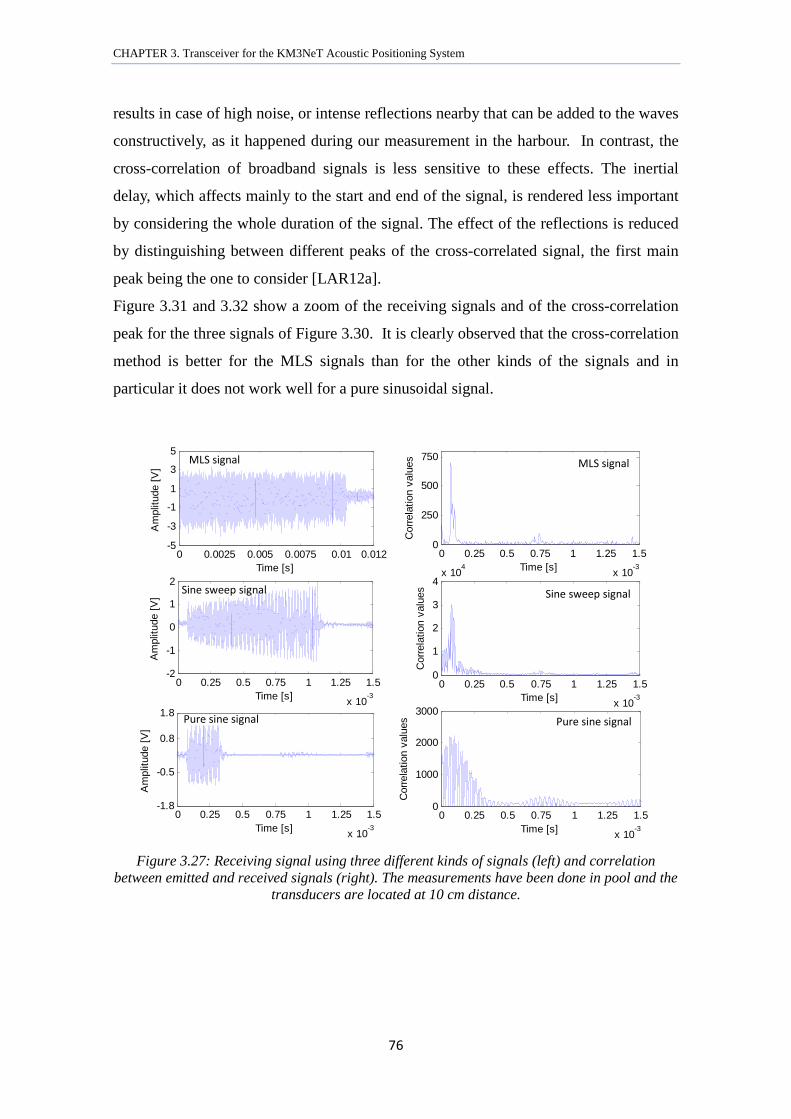
CHAPTER 3. Transceiver for the KM3NeT Acoustic Positioning System
76
results in case of high noise, or intense reflections nearby that can be added to the waves
constructively, as it happened during our measurement in the harbour. In contrast, the
cross-correlation of broadband signals is less sensitive to these effects. The inertial
delay, which affects mainly to the start and end of the signal, is rendered less important
by considering the whole duration of the signal. The effect of the reflections is reduced
by distinguishing between different peaks of the cross-correlated signal, the first main
peak being the one to consider [LAR12a].
Figure 3.31 and 3.32 show a zoom of the receiving signals and of the cross-correlation
peak for the three signals of Figure 3.30. It is clearly observed that the cross-correlation
method is better for the MLS signals than for the other kinds of the signals and in
particular it does not work well for a pure sinusoidal signal.
Figure 3.27: Receiving signal using three different kinds of signals (left) and correlation between emitted and received signals (right). The measurements have been done in pool and the
transducers are located at 10 cm distance.
0 0.0025 0.005 0.0075 0.01 0.012-5
-3
-1
1
3
5
Time [s]
Am
plitu
de [
V]
0 0.25 0.5 0.75 1 1.25 1.5
x 10-3
-2
-1
0
1
2
Time [s]
Am
plitu
de [
V]
0 0.25 0.5 0.75 1 1.25 1.5
x 10-3
-1.8
-0.5
0.8
1.8
Time [s]
Am
plitu
de [
V]
0 0.25 0.5 0.75 1 1.25 1.5
x 10-3
0
250
500
750
Time [s]
Cor
rela
tion
valu
es
0 0.25 0.5 0.75 1 1.25 1.5
x 10-3
0
1
2
3
4x 10
4
Time [s]
Cor
rela
tion
valu
es
0 0.25 0.5 0.75 1 1.25 1.5
x 10-3
0
1000
2000
3000
Time [s]
Cor
rela
tion
valu
es
MLS signal
Sine sweep signal
Pure sine signal
MLS signal
Sine sweep signal
Pure sine signal

CHAPTER 3. Transceiver for the KM3NeT Acoustic Positioning System
77
Figure 3.28: Receiving signal using three different kinds of signals (left) and correlation between emitted and received signals (right). The measurements have been done in pool and the
transducers are located at 1 m distance.
Figure 3.29: Receiving signal using three different kinds of signals (left) and correlation between emitted and received signals (right). The measurements have been done in harbour in
Gandia and the transducers are located at 4.50 m distance.
0 0.3 0.6 0.9 1.2 1.5 1.8 2
x 10-3
0
25
50
75
100
Time [s]
Cor
rela
tion
valu
es
0 0.3 0.6 0.9 1.2 1.5 1.8 2
x 10-3
0
1000
2000
3000
4000
Time [s]
Cor
rela
tion
valu
es
0 0.3 0.6 0.9 1.2 1.5 1.8 2
x 10-3
0
100
200
300
400
Time [s]
Cor
rela
tion
valu
es
0 0.0025 0.005 0.0075 0.01 0.012-2
-1
0
1
2
Time [s]
Am
plitu
de [
V]
0 0.3 0.6 0.9 1.2 1.5 1.8 2
x 10-3
-0.4
-0.2
0
0.2
0.4
Time [s]
Am
plitu
de [
V]
0 0.3 0.6 0.9 1.2 1.5 1.8 2
x 10-3
-0.4
-0.2
0
0.2
0.4
Time [s]
Am
plitu
de [
V]
0 1 2 3 4 5 6 7
x 10-3
0
110
220
330
440
Time [s]
Cor
rela
tion
valu
es
0 1 2 3 4 5 6 7
x 10-3
0
1.3
2.6
3.9
5
x 104
Time [s]
Cor
rela
tion
valu
es
0 1 2 3 4 5 6 7
x 10-3
0
280
560
840
1100
Time [s]
Cor
rela
tion
valu
es
0 0.0025 0.005 0.0075 0.01 0.012-4
-2
0
2
4
Time [s]
Am
plitu
de [
V]
0 1 2 3 4 5 6 7
x 10-3
-2
-1
0
1
2
Time [s]
Am
plitu
de [
V]
0 1 2 3 4 5 6 7
x 10-3
-4
-2
0
2
4
Time [s]
Am
plitu
de [
V]
MLS signal MLS signal
Sine sweep signal
Pure sine signal
Sine sweep signal
Pure sine signal
Pure sine signal
Sine sweep signal
MLS signal MLS signal
Sine sweep signal
Pure sine signal

CHAPTER 3. Transceiver for the KM3NeT Acoustic Positioning System
78
Figure 3.30: Receiving signal using three different kinds of signals (left) and correlation between emitted and received signals (right). The measurements have been done in harbor in
Gandia and the transducers are located at 140 m distance.
Figure 3.31: Zoom of the Receiving signal using three different kinds of signals (left) and zoom of the correlation between emitted and received signals (right). The measurements have been
done in harbor in Gandia and the transducers are located at 140 m distance.
0.05 0.065 0.08 0.095 0.11 0.125 0.14 0.15-3
-1
1
3
Time [s]
Am
plitu
de [
V]
0.05 0.065 0.08 0.095 0.11 0.125 0.14 0.15-1.5
-0.5
0.5
1.5
Time [s]
Am
plitu
de [
V]
0.05 0.065 0.08 0.095 0.11 0.125 0.14 0.15-2
-1
0
1
2
Time [s]
Am
plitu
de [
V]
0.05 0.065 0.08 0.095 0.11 0.125 0.140.150
250
500
700
Time [s]
Cor
rela
tion
valu
es
0.05 0.065 0.08 0.095 0.11 0.125 0.140.150
3.5
7
10x 10
4
Time [s]
Cor
rela
tion
valu
es
0.05 0.065 0.08 0.095 0.11 0.125 0.140.150
200
400
600
Time [s]
Cor
rela
tion
valu
es
0.08 0.084 0.088 0.092 0.096 0.1-3
-1.5
0
1.5
3
Time [s]
Am
plitu
de [
V]
0.08 0.084 0.088 0.092 0.096 0.1-1.5
-0.5
0.5
1.5
Time [s]
Am
plitu
de [
V]
0.08 0.084 0.088 0.092 0.096 0.1-1
-0.5
0
0.5
1
Time [s]
Am
plitu
de [
V]
0.08 0.084 0.088 0.092 0.096 0.10
250
500
700
Time [s]
Cor
rela
tion
valu
es
0.08 0.084 0.088 0.092 0.096 0.10
3.5
7
10x 10
4
Time [s]
Cor
rela
tion
valu
es
0.08 0.084 0.088 0.092 0.096 0.10
200
400
600
Time [s]
Cor
rela
tion
valu
es
Pure sine signal
Sine sweep signal
MLS signal MLS signal
Sine sweep signal
Pure sine signal
Pure sine signal
Sine sweep signal
MLS signal MLS signal
Sine sweep signal
Pure sine signal
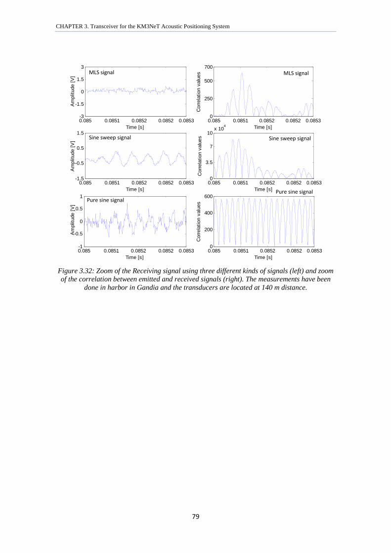
CHAPTER 3. Transceiver for the KM3NeT Acoustic Positioning System
79
Figure 3.32: Zoom of the Receiving signal using three different kinds of signals (left) and zoom of the correlation between emitted and received signals (right). The measurements have been
done in harbor in Gandia and the transducers are located at 140 m distance.
0.085 0.0851 0.0852 0.0852 0.0853-3
-1.5
0
1.5
3
Time [s]
Am
plitu
de [
V]
0.085 0.0851 0.0852 0.0852 0.0853-1.5
-0.5
0.5
1.5
Time [s]
Am
plitu
de [
V]
0.085 0.0851 0.0852 0.0852 0.0853-1
-0.5
0
0.5
1
Time [s]
Am
plitu
de [
V]
0.085 0.0851 0.0852 0.0852 0.08530
250
500
700
Time [s]
Cor
rela
tion
valu
es
0.085 0.0851 0.0852 0.0852 0.08530
3.5
7
10x 10
4
Time [s]
Cor
rela
tion
valu
es
0.085 0.0851 0.0852 0.0852 0.08530
200
400
600
Time [s]
Cor
rela
tion
valu
esPure sine signal
Sine sweep signal
MLS signal MLS signal
Sine sweep signal
Pure sine signal

80

CHAPTER 4. Integration of the acoustic transceiver in Underwater Neutrino Telescopes
81
Chapter 4
Integration of the acoustic transceiver in Underwater Neutrino
Telescopes
In this chapter the different activities and tests performed towards the integration of the
acoustic transceivers in neutrino telescopes infrastructures are presented. This will allow
for testing the acoustic transceiver in real conditions and studying their behaviour in
situ. Two different initiatives are presented: the integration in the instrumentation line of
ANTARES and the integration in the NEMO-Phase II tower.
4.1 Integration in ANTARES Neutrino Telescope
The acoustic transceiver presented in the previous chapter, already tested in the
laboratory, the pool and in Gandia Harbour, has been finally integrated in the active
anchor of the Instrumentation Line 07 (IL07), renamed IL11, of the ANTARES detector
on 3rd June 2011. The SEB was installed in a titanium container named Laser Container
holding also other electronic parts and the Laser Beacon system (LB) used for timing
calibration purposes. The Laser Container consists of a cylinder of 542 mm length and
with a diameter of 142 mm made of titanium grade 5 (Ti6AI4V). It is composed of three
different pieces: the cylindrical tube, the low cap (connector cap) and the upper cap with
the anti-biofouling system (described below). The inner aluminium mechanics provides
the structure where the different devices of the laser beacon are integrated. It consists of
two aluminium rings joined together by two aluminium beams. One of the rings is
screwed to the lower titanium end-cap. The drawings of this piece are shown in Figure
4.1. The anti-biofouling system is made by a diffuser disk and a quartz cylinder rod
which spreads light out following a cosine distribution over a half sphere (Figure 4.2).
The laser is needed for the timing calibration of a neutrino telescope and a new laser
will be tested in the IL.
The LB and the transducer were fixed on the active anchor through supports of
polyethylene designed and produced at the Instituto de Física Corpuscular, Valencia
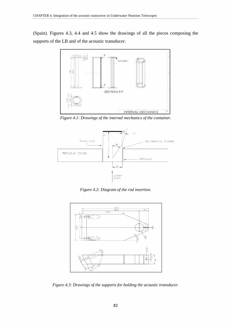
CHAPTER 4. Integration of the acoustic transceiver in Underwater Neutrino Telescopes
(Spain). Figures 4.3, 4.4 and 4.5 show the
supports of the LB and of the acoustic transducer.
Figure 4.1: Drawings of the internal mechanics of the container.
Figure 4.2: Diagram
Figure 4.3: Drawings of the
acoustic transceiver in Underwater Neutrino Telescopes
82
(Spain). Figures 4.3, 4.4 and 4.5 show the drawings of all the pieces
supports of the LB and of the acoustic transducer.
Figure 4.1: Drawings of the internal mechanics of the container.
Figure 4.2: Diagram of the rod insertion.
Drawings of the supports for holding the acoustic transducer.
drawings of all the pieces composing the
Figure 4.1: Drawings of the internal mechanics of the container.
for holding the acoustic transducer.
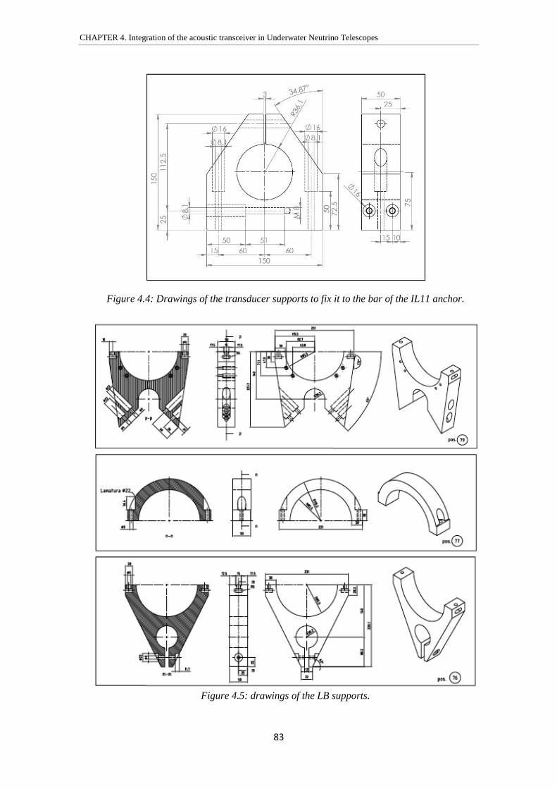
CHAPTER 4. Integration of the acoustic transceiver in Underwater Neutrino Telescopes
83
Figure 4.4: Drawings of the transducer supports to fix it to the bar of the IL11 anchor.
Figure 4.5: drawings of the LB supports.
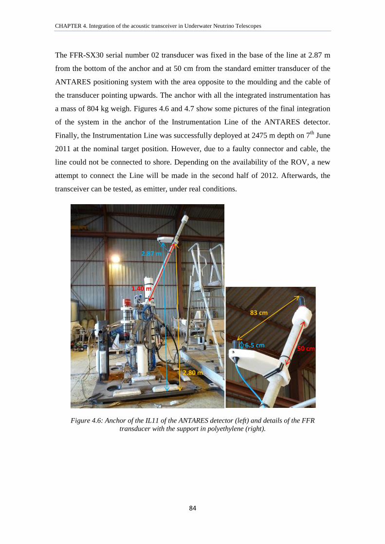
CHAPTER 4. Integration of the acoustic transceiver in Underwater Neutrino Telescopes
84
The FFR-SX30 serial number 02 transducer was fixed in the base of the line at 2.87 m
from the bottom of the anchor and at 50 cm from the standard emitter transducer of the
ANTARES positioning system with the area opposite to the moulding and the cable of
the transducer pointing upwards. The anchor with all the integrated instrumentation has
a mass of 804 kg weigh. Figures 4.6 and 4.7 show some pictures of the final integration
of the system in the anchor of the Instrumentation Line of the ANTARES detector.
Finally, the Instrumentation Line was successfully deployed at 2475 m depth on 7th June
2011 at the nominal target position. However, due to a faulty connector and cable, the
line could not be connected to shore. Depending on the availability of the ROV, a new
attempt to connect the Line will be made in the second half of 2012. Afterwards, the
transceiver can be tested, as emitter, under real conditions.
Figure 4.6: Anchor of the IL11 of the ANTARES detector (left) and details of the FFR transducer with the support in polyethylene (right).
50 cm
83 cm
2.87 m
2.80 m
1.40 m
6.5 cm
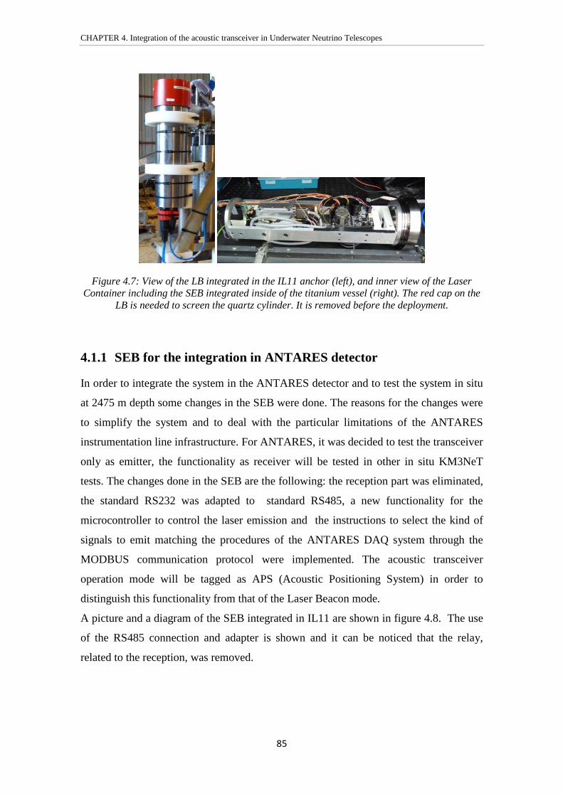
CHAPTER 4. Integration of the acoustic transceiver in Underwater Neutrino Telescopes
85
Figure 4.7: View of the LB integrated in the IL11 anchor (left), and inner view of the Laser Container including the SEB integrated inside of the titanium vessel (right). The red cap on the
LB is needed to screen the quartz cylinder. It is removed before the deployment.
4.1.1 SEB for the integration in ANTARES detector
In order to integrate the system in the ANTARES detector and to test the system in situ
at 2475 m depth some changes in the SEB were done. The reasons for the changes were
to simplify the system and to deal with the particular limitations of the ANTARES
instrumentation line infrastructure. For ANTARES, it was decided to test the transceiver
only as emitter, the functionality as receiver will be tested in other in situ KM3NeT
tests. The changes done in the SEB are the following: the reception part was eliminated,
the standard RS232 was adapted to standard RS485, a new functionality for the
microcontroller to control the laser emission and the instructions to select the kind of
signals to emit matching the procedures of the ANTARES DAQ system through the
MODBUS communication protocol were implemented. The acoustic transceiver
operation mode will be tagged as APS (Acoustic Positioning System) in order to
distinguish this functionality from that of the Laser Beacon mode.
A picture and a diagram of the SEB integrated in IL11 are shown in figure 4.8. The use
of the RS485 connection and adapter is shown and it can be noticed that the relay,
related to the reception, was removed.
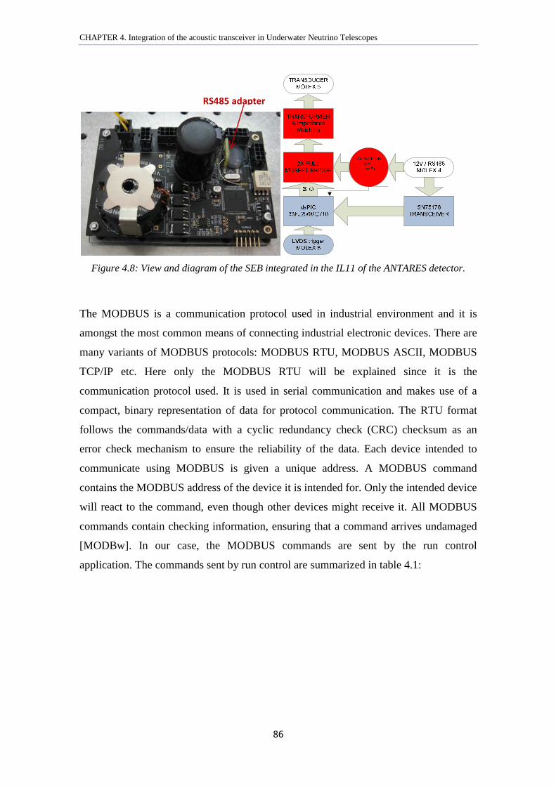
CHAPTER 4. Integration of the acoustic transceiver in Underwater Neutrino Telescopes
86
Figure 4.8: View and diagram of the SEB integrated in the IL11 of the ANTARES detector.
The MODBUS is a communication protocol used in industrial environment and it is
amongst the most common means of connecting industrial electronic devices. There are
many variants of MODBUS protocols: MODBUS RTU, MODBUS ASCII, MODBUS
TCP/IP etc. Here only the MODBUS RTU will be explained since it is the
communication protocol used. It is used in serial communication and makes use of a
compact, binary representation of data for protocol communication. The RTU format
follows the commands/data with a cyclic redundancy check (CRC) checksum as an
error check mechanism to ensure the reliability of the data. Each device intended to
communicate using MODBUS is given a unique address. A MODBUS command
contains the MODBUS address of the device it is intended for. Only the intended device
will react to the command, even though other devices might receive it. All MODBUS
commands contain checking information, ensuring that a command arrives undamaged
[MODBw]. In our case, the MODBUS commands are sent by the run control
application. The commands sent by run control are summarized in table 4.1:
RS485 adapter
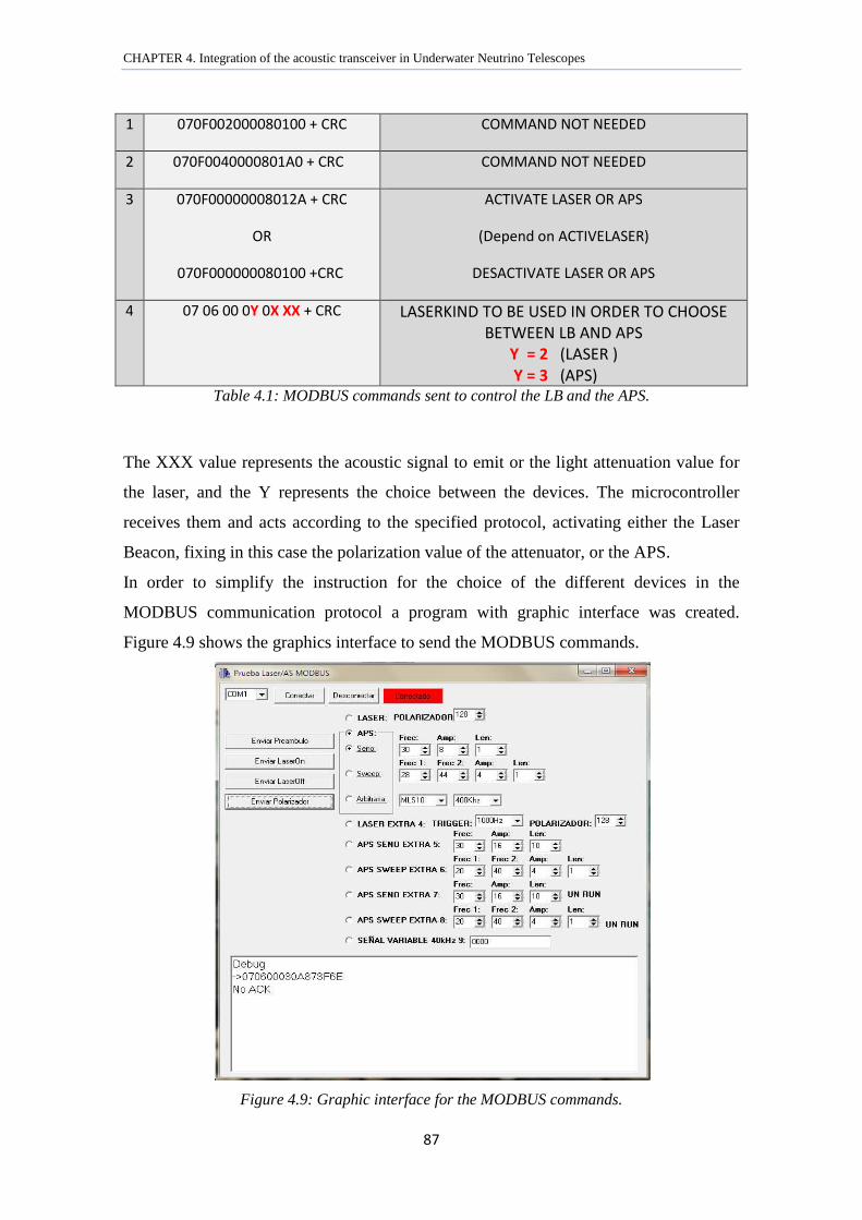
CHAPTER 4. Integration of the acoustic transceiver in Underwater Neutrino Telescopes
87
1 070F002000080100 + CRC COMMAND NOT NEEDED
2 070F0040000801A0 + CRC COMMAND NOT NEEDED
3 070F00000008012A + CRC
OR
070F000000080100 +CRC
ACTIVATE LASER OR APS
(Depend on ACTIVELASER)
DESACTIVATE LASER OR APS
4 07 06 00 0Y 0X XX + CRC LASERKIND TO BE USED IN ORDER TO CHOOSE
BETWEEN LB AND APS Y = 2 (LASER )
Y = 3 (APS)
Table 4.1: MODBUS commands sent to control the LB and the APS.
The XXX value represents the acoustic signal to emit or the light attenuation value for
the laser, and the Y represents the choice between the devices. The microcontroller
receives them and acts according to the specified protocol, activating either the Laser
Beacon, fixing in this case the polarization value of the attenuator, or the APS.
In order to simplify the instruction for the choice of the different devices in the
MODBUS communication protocol a program with graphic interface was created.
Figure 4.9 shows the graphics interface to send the MODBUS commands.
Figure 4.9: Graphic interface for the MODBUS commands.
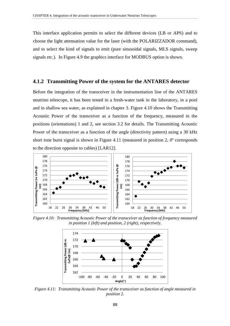
CHAPTER 4. Integration of the acoustic transceiver in Underwater Neutrino Telescopes
88
This interface application permits to select the different devices (LB or APS) and to
choose the light attenuation value for the laser (with the POLARIZZADOR command),
and to select the kind of signals to emit (pure sinusoidal signals, MLS signals, sweep
signals etc.). In Figure 4.9 the graphics interface for MODBUS option is shown.
4.1.2 Transmitting Power of the system for the ANTARES detector
Before the integration of the transceiver in the instrumentation line of the ANTARES
neutrino telescope, it has been tested in a fresh-water tank in the laboratory, in a pool
and in shallow sea water, as explained in chapter 3. Figure 4.10 shows the Transmitting
Acoustic Power of the transceiver as a function of the frequency, measured in the
positions (orientations) 1 and 2, see section 3.2 for details. The Transmitting Acoustic
Power of the transceiver as a function of the angle (directivity pattern) using a 30 kHz
short tone burst signal is shown in Figure 4.11 (measured in position 2, 0º corresponds
to the direction opposite to cables) [LAR12].
Figure 4.10: Transmitting Acoustic Power of the transceiver as function of frequency measured in position 1 (left) and position, 2 (right), respectively.
Figure 4.11: Transmitting Acoustic Power of the transceiver as function of angle measured in position 2.
160
162
164
166
168
170
172
174
176
178
180
18 22 26 30 34 38 42 46 50
Tra
nsm
itti
ng
Po
we
r (r
e 1
uP
a @
1m
)
Frequency [kHz]
160
162
164
166
168
170
172
174
176
178
180
18 22 26 30 34 38 42 46 50Tra
nsm
itti
ng
Po
we
r (d
B r
e 1
uP
a @
1m
)
Frequency [kHz]
162
164
166
168
170
172
174
-100 -80 -60 -40 -20 0 20 40 60 80 100
Tra
nsm
itti
ng
Po
we
r (d
B r
e
1u
Pa
@ 1
m)
Angle[°]
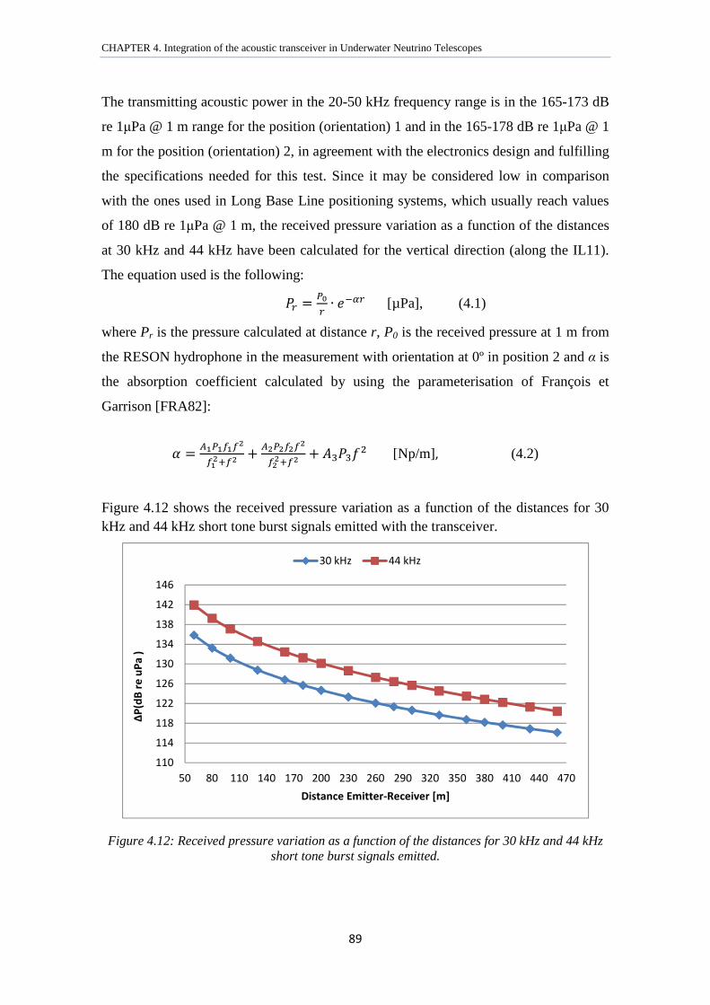
CHAPTER 4. Integration of the acoustic transceiver in Underwater Neutrino Telescopes
89
The transmitting acoustic power in the 20-50 kHz frequency range is in the 165-173 dB
re 1µPa @ 1 m range for the position (orientation) 1 and in the 165-178 dB re 1µPa @ 1
m for the position (orientation) 2, in agreement with the electronics design and fulfilling
the specifications needed for this test. Since it may be considered low in comparison
with the ones used in Long Base Line positioning systems, which usually reach values
of 180 dB re 1µPa @ 1 m, the received pressure variation as a function of the distances
at 30 kHz and 44 kHz have been calculated for the vertical direction (along the IL11).
The equation used is the following:
=
∙ [µPa], (4.1)
where Pr is the pressure calculated at distance r, P0 is the received pressure at 1 m from
the RESON hydrophone in the measurement with orientation at 0º in position 2 and α is
the absorption coefficient calculated by using the parameterisation of François et
Garrison [FRA82]:
=
+
+ [Np/m], (4.2)
Figure 4.12 shows the received pressure variation as a function of the distances for 30 kHz and 44 kHz short tone burst signals emitted with the transceiver.
Figure 4.12: Received pressure variation as a function of the distances for 30 kHz and 44 kHz short tone burst signals emitted.
110
114
118
122
126
130
134
138
142
146
50 80 110 140 170 200 230 260 290 320 350 380 410 440 470
ΔP
(dB
re
uP
a )
Distance Emitter-Receiver [m]
30 kHz 44 kHz

CHAPTER 4. Integration of the acoustic transceiver in Underwater Neutrino Telescopes
90
The results show clearly that the pressure decreases with distance until 116 dB re µPa
and 120 dB re µPa at 460 m for 30 kHz and 44 kHz tone burst signals respectively.
Successively, these data have been used to calculate the received electric signal
amplitude that would be measured the AMADEUS and ANTARES hydrophones,
knowing that the sensitivity for the AMADEUS hydrophone is -145.5 dB re 1V/µPa at
30 kHz and for the ANTARES hydrophone is -196 dB re 1V/µPa at 44kHz. Figures
4.13 and 4.14 show the received amplitude calculated for the AMADEUS and
ANTARES hydrophones, respectively.
Figure 4.13: Received amplitude with the AMADEUS hydrophones at 30 kHz frequency. In the IL07 (IL11), the AMADEUS hydrophones are located at distances of 180 m, 195 m and 305 m.
Figure 4.14: Received amplitude with the ANTARES hydrophone at 44 kHz frequency.
24
54
84
114
144
174
204
234
264
294
324
354
50 80 110 140 170 200 230 260 290 320 350 380 410 440 470
Am
pli
tud
e [
mV
]
Distance Emitter-Receiver [m]
0
0,2
0,4
0,6
0,8
1
1,2
1,4
1,6
1,8
2
2,2
2,4
50 80 110 140 170 200 230 260 290 320 350 380 410 440 470
Am
pli
tud
e [
mV
]
Distance Emitter-Receiver [m]

CHAPTER 4. Integration of the acoustic transceiver in Underwater Neutrino Telescopes
91
The results show that at 460 m signals with amplitudes of about 34 mV and 0.2 mV for
the AMADEUS and ANTARES hydrophone, respectively, are expected. Considering
that the last storey in the IL with AMADEUS hydrophones is located at 305 m above
the sea floor, the signal measured will be of about 57 mV amplitude, enough to be
recorded above the ambient noise. Whereas for the ANTARES hydrophones the results
show that the signal amplitude is weak and difficult to be useful for long distances.
Moreover, the received pressure variation and the electric signal amplitude expected for
the AMADEUS hydrophones on the Line 12 for a 30 kHz short tone burst signal
emitted with the transceiver have also been calculated and shown in figure 4.15. The
orientation of the emitter and receivers has been taken into account (it corresponds to an
angle of ~60º with position 2). Here, again the expected electric signal is enough to be
recorded above the noise.
Figure 4.15: Pressure variation (left) and expected electric signal amplitude (right) for the AMADEUS hydrophones of Line12 floor 21-23 using 30 kHz tone burst signals.
Following these results, we can consider that the integration of the emitter in the IL of
ANTARES is very important in order to test it in situ and validate it for deep sea
conditions. The use of the transceiver in combination with the AMADEUS hydrophones
makes the test very complete since it allows studying the transceiver emission for
different conditions of distances and orientation. Moreover, it is possible to study in situ
different kind of signals (tone bursts at different frequencies, but also broadband
frequency signals such as MLS or sine sweeps) and conclude about the possibility of
110
111
112
113
114
115
116
440 450 460 470 480
ΔP
(dB
re
uP
a )
Distance Emitter-Receiver [m]
30 kHz
20
22
24
26
28
30
440 450 460 470 480
Am
pli
tud
e [
mV
]
Distance Emitter-Receiver [m]
30kHz
Floor 21
Floor 22 Floor 23
Floor 21
Floor 22
Floor 23

CHAPTER 4. Integration of the acoustic transceiver in Underwater Neutrino Telescopes
92
improving the signal to noise ratio (and therefore being able to cover longer distances)
by using broadband frequency signals.
4.2 Integration in NEMO detector
The transceiver prototype system is also already available to be integrated in the base of
the NEMO Phase II tower. The integration is estimated by July 2012. The system is
composed of a moulded FFR-SX30 transducer, serial number 566, and a Sound
Emission Board as described in sections 3.1.1 and 3.1.2, respectively. Furthermore, two
other FFR transducers, with serial numbers 788 and 05, will be integrated as receiver in
different floors of the tower. The latter were connected to a SMID AM-401 preamplifier
[SMIDw] with 20 x 80 mm2 of dimension and 38 dB gain and the whole receiver
moulded by SEACON (europe) Ltd [SEACw]. The moulding and the cable are both in
polyurethane. Figure 4.16 shows the FFR-SX30 moulded from by SEACON together
with the SMID preamplifier. Tests performed at INFN-LNS have demonstrated the full
compatibility of the sensors with the SMID AM-401 preamplifier [VIO12]. These
sensors together with 2 piezo-sensors developed by ECAP, 14 further high sensitivity
and broadband SMID hydrophones and the transceiver prototype will constitute the
APS prototype to be tested in NEMO-Phase II.
Figure 4.16: A picture of the two hydrophones (FFR-SX30 with SMID preamplifier) moulded by SEACON.
As in the case of the integration in the ANTARES detector (Figures 4.1 and 4.2), the
transceiver here will be tested only as emitter and in connection with the Laser Beacon
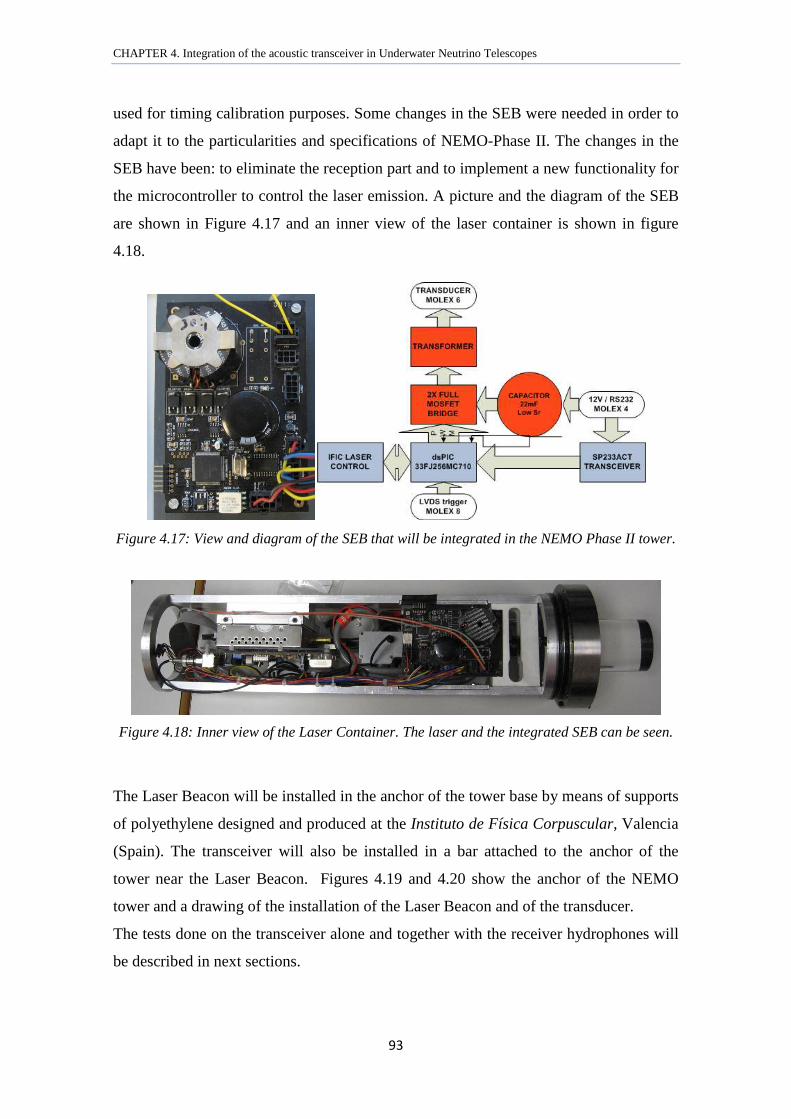
CHAPTER 4. Integration of the acoustic transceiver in Underwater Neutrino Telescopes
93
used for timing calibration purposes. Some changes in the SEB were needed in order to
adapt it to the particularities and specifications of NEMO-Phase II. The changes in the
SEB have been: to eliminate the reception part and to implement a new functionality for
the microcontroller to control the laser emission. A picture and the diagram of the SEB
are shown in Figure 4.17 and an inner view of the laser container is shown in figure
4.18.
Figure 4.17: View and diagram of the SEB that will be integrated in the NEMO Phase II tower.
Figure 4.18: Inner view of the Laser Container. The laser and the integrated SEB can be seen.
The Laser Beacon will be installed in the anchor of the tower base by means of supports
of polyethylene designed and produced at the Instituto de Física Corpuscular, Valencia
(Spain). The transceiver will also be installed in a bar attached to the anchor of the
tower near the Laser Beacon. Figures 4.19 and 4.20 show the anchor of the NEMO
tower and a drawing of the installation of the Laser Beacon and of the transducer.
The tests done on the transceiver alone and together with the receiver hydrophones will
be described in next sections.
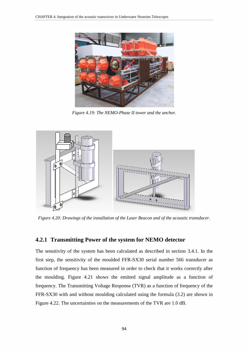
CHAPTER 4. Integration of the acoustic transceiver in Underwater Neutrino Telescopes
94
Figure 4.19: The NEMO-Phase II tower and the anchor.
Figure 4.20: Drawings of the installation of the Laser Beacon and of the acoustic transducer.
4.2.1 Transmitting Power of the system for NEMO detector
The sensitivity of the system has been calculated as described in section 3.4.1. In the
first step, the sensitivity of the moulded FFR-SX30 serial number 566 transducer as
function of frequency has been measured in order to check that it works correctly after
the moulding. Figure 4.21 shows the emitted signal amplitude as a function of
frequency. The Transmitting Voltage Response (TVR) as a function of frequency of the
FFR-SX30 with and without moulding calculated using the formula (3.2) are shown in
Figure 4.22. The uncertainties on the measurements of the TVR are 1.0 dB.
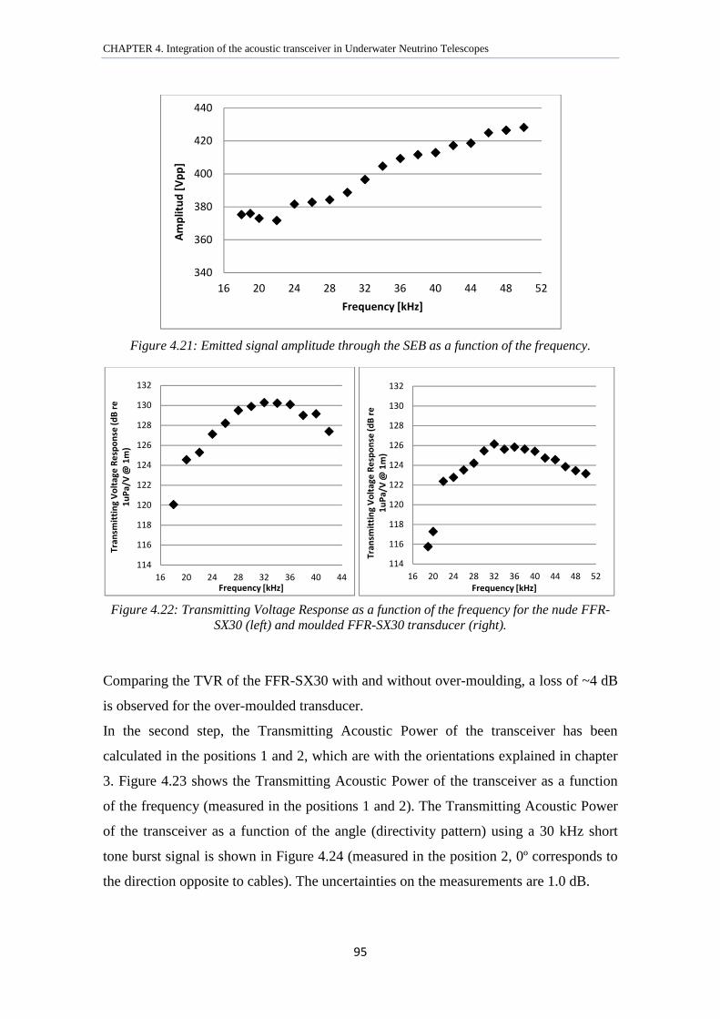
CHAPTER 4. Integration of the acoustic transceiver in Underwater Neutrino Telescopes
95
Figure 4.21: Emitted signal amplitude through the SEB as a function of the frequency.
Figure 4.22: Transmitting Voltage Response as a function of the frequency for the nude FFR-
SX30 (left) and moulded FFR-SX30 transducer (right).
Comparing the TVR of the FFR-SX30 with and without over-moulding, a loss of ~4 dB
is observed for the over-moulded transducer.
In the second step, the Transmitting Acoustic Power of the transceiver has been
calculated in the positions 1 and 2, which are with the orientations explained in chapter
3. Figure 4.23 shows the Transmitting Acoustic Power of the transceiver as a function
of the frequency (measured in the positions 1 and 2). The Transmitting Acoustic Power
of the transceiver as a function of the angle (directivity pattern) using a 30 kHz short
tone burst signal is shown in Figure 4.24 (measured in the position 2, 0º corresponds to
the direction opposite to cables). The uncertainties on the measurements are 1.0 dB.
340
360
380
400
420
440
16 20 24 28 32 36 40 44 48 52
Am
pli
tud
[V
pp
]
Frequency [kHz]
114
116
118
120
122
124
126
128
130
132
16 20 24 28 32 36 40 44
Tra
nsm
itti
ng
Vo
lta
ge
Re
spo
nse
(d
B r
e
1u
Pa
/V @
1m
)
Frequency [kHz]
114
116
118
120
122
124
126
128
130
132
16 20 24 28 32 36 40 44 48 52
Tra
nsm
itti
ng
Vo
lta
ge
Re
spo
nse
(d
B r
e
1u
Pa
/V @
1m
)
Frequency [kHz]
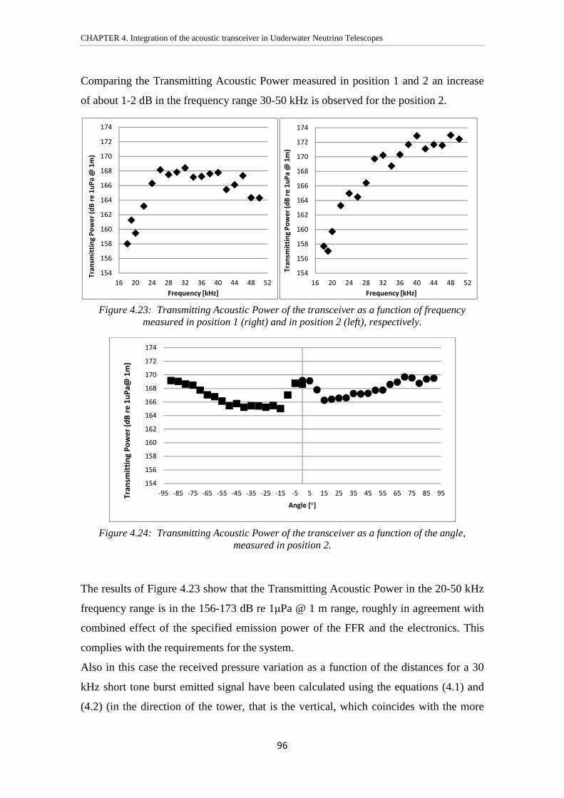
CHAPTER 4. Integration of the acoustic transceiver in Underwater Neutrino Telescopes
96
Comparing the Transmitting Acoustic Power measured in position 1 and 2 an increase
of about 1-2 dB in the frequency range 30-50 kHz is observed for the position 2.
Figure 4.23: Transmitting Acoustic Power of the transceiver as a function of frequency
measured in position 1 (right) and in position 2 (left), respectively.
Figure 4.24: Transmitting Acoustic Power of the transceiver as a function of the angle,
measured in position 2.
The results of Figure 4.23 show that the Transmitting Acoustic Power in the 20-50 kHz
frequency range is in the 156-173 dB re 1µPa @ 1 m range, roughly in agreement with
combined effect of the specified emission power of the FFR and the electronics. This
complies with the requirements for the system.
Also in this case the received pressure variation as a function of the distances for a 30
kHz short tone burst emitted signal have been calculated using the equations (4.1) and
(4.2) (in the direction of the tower, that is the vertical, which coincides with the more
154
156
158
160
162
164
166
168
170
172
174
16 20 24 28 32 36 40 44 48 52
Tra
nsm
itti
ng
Po
we
r (d
B r
e 1
uP
a @
1m
)
Frequency [kHz]
154
156
158
160
162
164
166
168
170
172
174
16 20 24 28 32 36 40 44 48 52T
ran
smit
tin
g P
ow
er
(dB
re
1u
Pa
@ 1
m)
Frequency [kHz]
154
156
158
160
162
164
166
168
170
172
174
-95 -85 -75 -65 -55 -45 -35 -25 -15 -5 5 15 25 35 45 55 65 75 85 95Tra
nsm
itti
ng
Po
we
r (d
B r
e 1
uP
a@
1m
)
Angle [°]
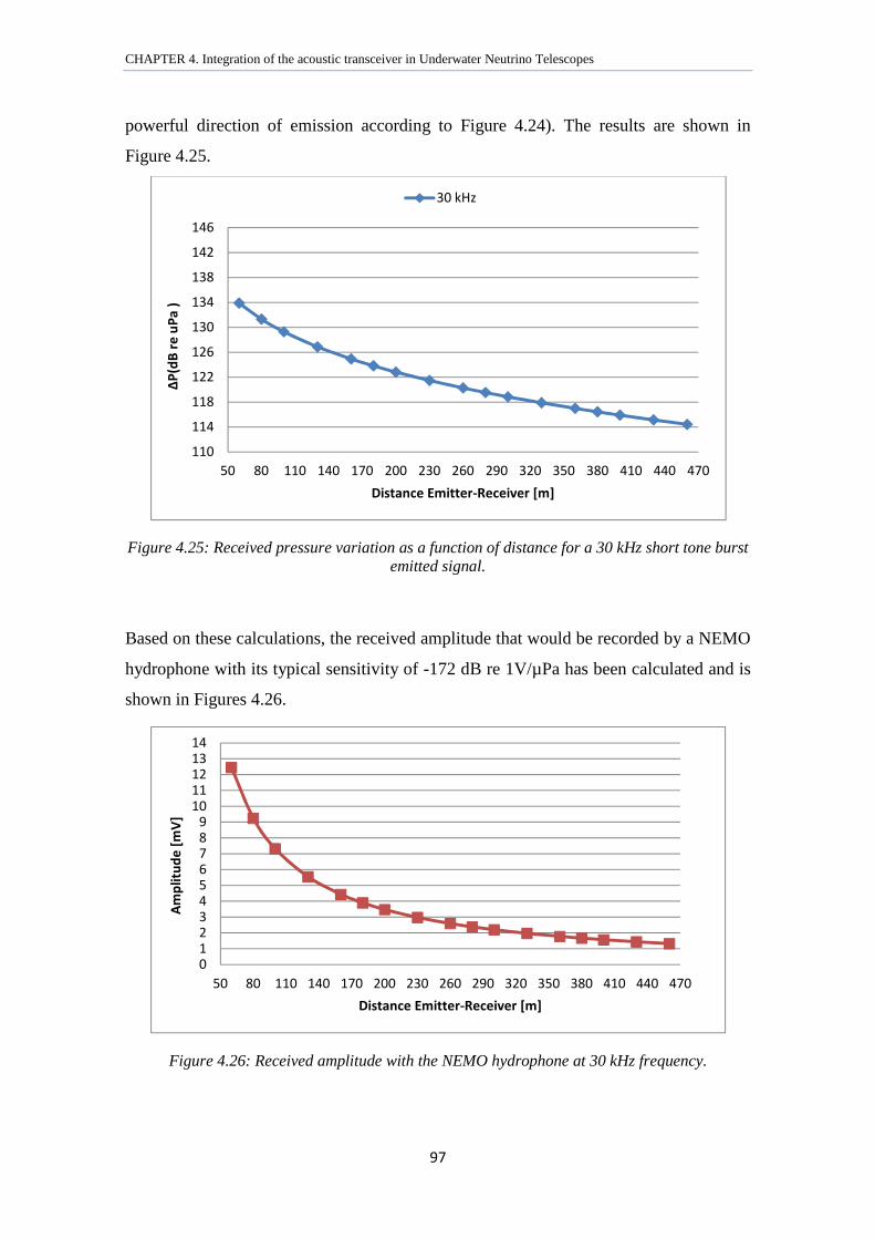
CHAPTER 4. Integration of the acoustic transceiver in Underwater Neutrino Telescopes
97
powerful direction of emission according to Figure 4.24). The results are shown in
Figure 4.25.
Figure 4.25: Received pressure variation as a function of distance for a 30 kHz short tone burst emitted signal.
Based on these calculations, the received amplitude that would be recorded by a NEMO
hydrophone with its typical sensitivity of -172 dB re 1V/µPa has been calculated and is
shown in Figures 4.26.
Figure 4.26: Received amplitude with the NEMO hydrophone at 30 kHz frequency.
110
114
118
122
126
130
134
138
142
146
50 80 110 140 170 200 230 260 290 320 350 380 410 440 470
ΔP
(dB
re
uP
a )
Distance Emitter-Receiver [m]
30 kHz
0123456789
1011121314
50 80 110 140 170 200 230 260 290 320 350 380 410 440 470
Am
pli
tud
e [
mV
]
Distance Emitter-Receiver [m]

CHAPTER 4. Integration of the acoustic transceiver in Underwater Neutrino Telescopes
98
The results show that at 460 m the expected signal has an amplitude of about 1.3 mV
for the NEMO hydrophones. Considering that the last storey in the NEMO Phase II is
located at 420 m above the sea floor, the expected signal will have amplitude of about
1.6 mV, enough to be recorded above the ambient noise.
4.2.2 NEMO Phase II joint acoustic tests
The compatibility and functionality of different hardware and software for the NEMO
Phase II test (developed by INFN-Italy, CPPM-France, ECAP-Germany and UPV-
Spain towards an innovative APS within the KM3NeT Consortium) were performed in
a joint acoustic test in the laboratory in Gandia in May 2010. In these tests the
compatibility and functionality between the acquisition electronic chains NEMO and
the transceiver (FFR-SX30 plus SEB) were successfully tested. Details about the joint
acoustic tests can be found in [SIM12].
In order to evaluate and compare the performances in water of the two SMID and FFR-
SX30 hydrophones and of the transceiver for the integration in NEMO Phase II tower,
tests in a fresh water pool of dimensions 4 x 6 x 5.30 m have been performed at IDASC
(Istituto di Acustica e Sensoristica “Orso Mario Corbino”) [IDASw] in Rome (Figure
4.27).
Figure 4.27: Fresh water pool at IDASC (Istituto di Acustica e Sensoristica “Orso Mario Corbino”) with dimension of 4 x 6 x 5.30 m.
4 m
6 m

CHAPTER 4. Integration of the acoustic transceiver in Underwater Neutrino Telescopes
99
The transducers have been placed in the water pool at different positions and known
distances from the acoustic sources by means of carbon fibre bars provided by IDASC
and mechanical supports of polyethylene designed and produced at the INFN (Istituto
Nazionale di Fisica Nucleare), Catania (Italy). Maintaining a similar notation to that of
chapter 3, the different configurations of the measurements have been named position 1
and 2 as shown in Figure 4.28. The receiver hydrophones were connected to the data
acquisition system of the NEMO detector. The set up used for the emission, reception
and acquisition of data is shown in Figure 4.29.
Figure 4.28: Experimental setup for the acoustic measurements in water pool at IDASC. Position 1 on left and position 2 on right. Emitter ITC 1032 and Receivers FFR-SX30 788 and
05, and SMID H1 and H2.
The emitted signal was generated through a signal generator and sent to the transducer
(ITC 1032) for the emission. The trigger of the signal generator was managed from GPS
with a signal named PPS (Pulse Per Second). The latter provide in output two channel
one for the clock and another for the IRIG code data (year, month, day, etc.).
Furthermore, it was connected to the Fan Time board in order to distribute the master
clock (that is, the clock at 10MHz of the receiver GPS) and GPS time to electronic
Position 1
120 cm
788
05
H1
H2 121.5 cm
122.5 cm
114.4 cm
114.9 cm
Position 2
788
H1
H2
05
Equator of the ITC
142.8 cm
152 cm
151.5 cm
141.5 cm
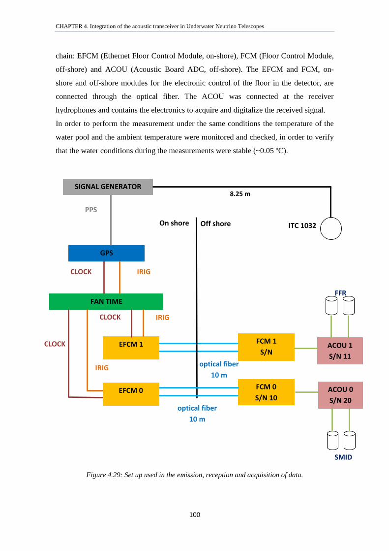
CHAPTER 4. Integration of the acoustic transceiver in Underwater Neutrino Telescopes
100
chain: EFCM (Ethernet Floor Control Module, on-shore), FCM (Floor Control Module,
off-shore) and ACOU (Acoustic Board ADC, off-shore). The EFCM and FCM, on-
shore and off-shore modules for the electronic control of the floor in the detector, are
connected through the optical fiber. The ACOU was connected at the receiver
hydrophones and contains the electronics to acquire and digitalize the received signal.
In order to perform the measurement under the same conditions the temperature of the
water pool and the ambient temperature were monitored and checked, in order to verify
that the water conditions during the measurements were stable (~0.05 ºC).
Figure 4.29: Set up used in the emission, reception and acquisition of data.
GPS
FAN TIME
EFCM 1 FCM 1
S/N ACOU 1
S/N 11 optical fiber
10 m
On shore Off shore
IRIG
CLOCK
IRIG
FFR
SMID
EFCM 0 FCM 0
S/N 10 ACOU 0
S/N 20 optical fiber
10 m
IRIG
CLOCK
CLOCK
SIGNAL GENERATOR
PPS
ITC 1032
8.25 m
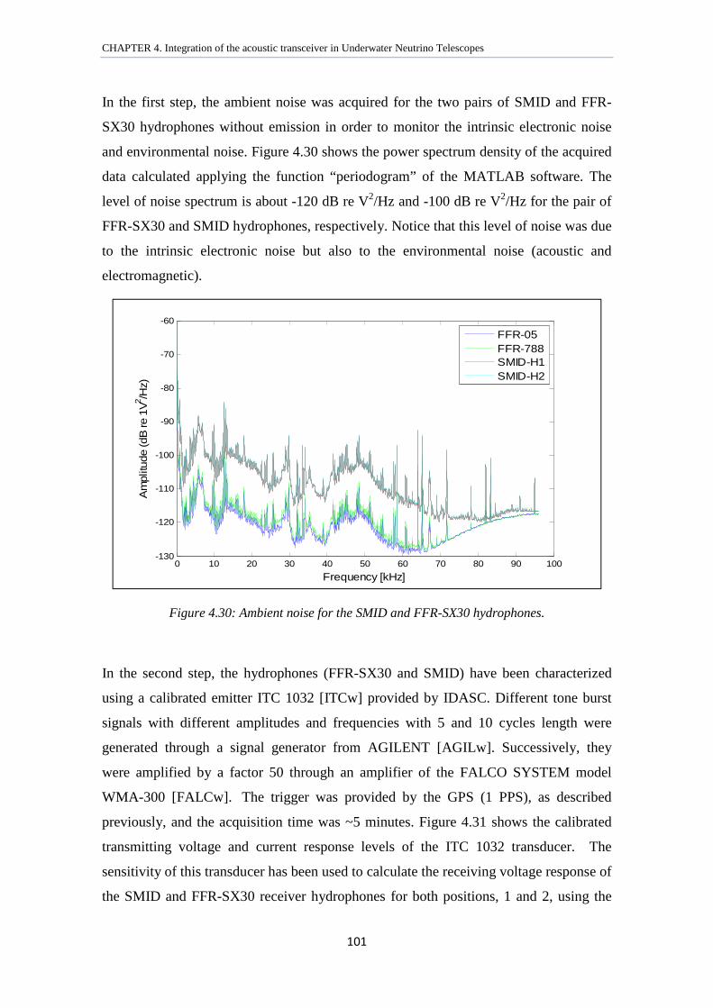
CHAPTER 4. Integration of the acoustic transceiver in Underwater Neutrino Telescopes
101
In the first step, the ambient noise was acquired for the two pairs of SMID and FFR-
SX30 hydrophones without emission in order to monitor the intrinsic electronic noise
and environmental noise. Figure 4.30 shows the power spectrum density of the acquired
data calculated applying the function “periodogram” of the MATLAB software. The
level of noise spectrum is about -120 dB re V2/Hz and -100 dB re V2/Hz for the pair of
FFR-SX30 and SMID hydrophones, respectively. Notice that this level of noise was due
to the intrinsic electronic noise but also to the environmental noise (acoustic and
electromagnetic).
Figure 4.30: Ambient noise for the SMID and FFR-SX30 hydrophones.
In the second step, the hydrophones (FFR-SX30 and SMID) have been characterized
using a calibrated emitter ITC 1032 [ITCw] provided by IDASC. Different tone burst
signals with different amplitudes and frequencies with 5 and 10 cycles length were
generated through a signal generator from AGILENT [AGILw]. Successively, they
were amplified by a factor 50 through an amplifier of the FALCO SYSTEM model
WMA-300 [FALCw]. The trigger was provided by the GPS (1 PPS), as described
previously, and the acquisition time was ~5 minutes. Figure 4.31 shows the calibrated
transmitting voltage and current response levels of the ITC 1032 transducer. The
sensitivity of this transducer has been used to calculate the receiving voltage response of
the SMID and FFR-SX30 receiver hydrophones for both positions, 1 and 2, using the
0 10 20 30 40 50 60 70 80 90 100-130
-120
-110
-100
-90
-80
-70
-60
Frequency [kHz]
Am
plitu
de (d
B re
1V2 /H
z)
FFR-05FFR-788SMID-H1SMID-H2
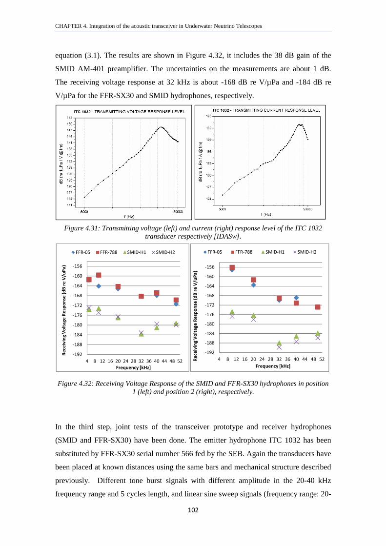
CHAPTER 4. Integration of the acoustic transceiver in Underwater Neutrino Telescopes
102
equation (3.1). The results are shown in Figure 4.32, it includes the 38 dB gain of the
SMID AM-401 preamplifier. The uncertainties on the measurements are about 1 dB.
The receiving voltage response at 32 kHz is about -168 dB re V/µPa and -184 dB re
V/µPa for the FFR-SX30 and SMID hydrophones, respectively.
Figure 4.31: Transmitting voltage (left) and current (right) response level of the ITC 1032 transducer respectively [IDASw].
Figure 4.32: Receiving Voltage Response of the SMID and FFR-SX30 hydrophones in position 1 (left) and position 2 (right), respectively.
In the third step, joint tests of the transceiver prototype and receiver hydrophones
(SMID and FFR-SX30) have been done. The emitter hydrophone ITC 1032 has been
substituted by FFR-SX30 serial number 566 fed by the SEB. Again the transducers have
been placed at known distances using the same bars and mechanical structure described
previously. Different tone burst signals with different amplitude in the 20-40 kHz
frequency range and 5 cycles length, and linear sine sweep signals (frequency range: 20-
-192
-188
-184
-180
-176
-172
-168
-164
-160
-156
4 8 12 16 20 24 28 32 36 40 44 48 52
Re
ceiv
ing
Vo
lta
ge
Re
spo
nse
(d
B r
e V
/uP
a)
Frequency [kHz]
FFR-05 FFR-788 SMID-H1 SMID-H2
-192
-188
-184
-180
-176
-172
-168
-164
-160
-156
4 8 12 16 20 24 28 32 36 40 44 48 52Re
ceiv
ing
Vo
lta
ge
Re
spo
nse
(d
B r
e V
/uP
a)
Frequency [kHz]
FFR-05 FFR-788 SMID-H1 SMID-H2
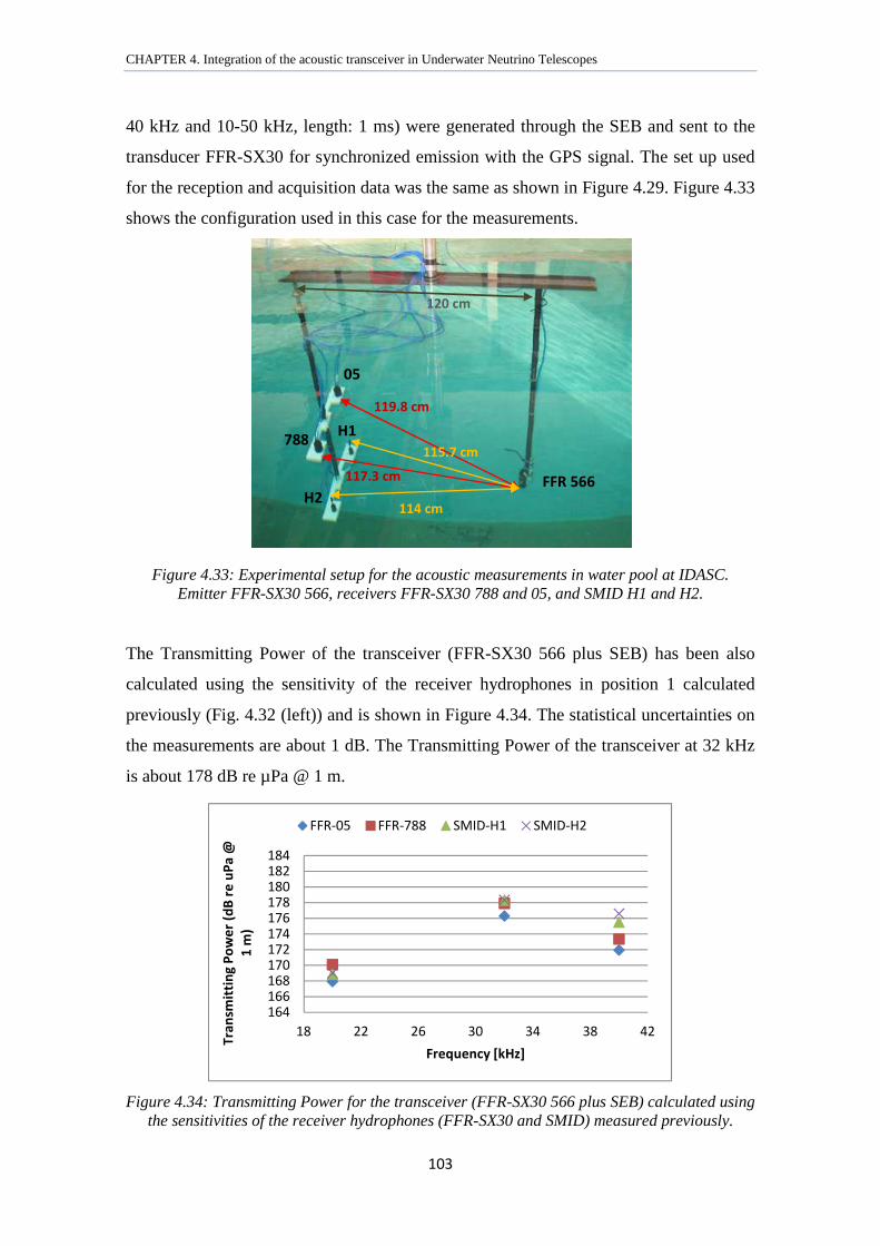
CHAPTER 4. Integration of the acoustic transceiver in Underwater Neutrino Telescopes
103
40 kHz and 10-50 kHz, length: 1 ms) were generated through the SEB and sent to the
transducer FFR-SX30 for synchronized emission with the GPS signal. The set up used
for the reception and acquisition data was the same as shown in Figure 4.29. Figure 4.33
shows the configuration used in this case for the measurements.
Figure 4.33: Experimental setup for the acoustic measurements in water pool at IDASC. Emitter FFR-SX30 566, receivers FFR-SX30 788 and 05, and SMID H1 and H2.
The Transmitting Power of the transceiver (FFR-SX30 566 plus SEB) has been also
calculated using the sensitivity of the receiver hydrophones in position 1 calculated
previously (Fig. 4.32 (left)) and is shown in Figure 4.34. The statistical uncertainties on
the measurements are about 1 dB. The Transmitting Power of the transceiver at 32 kHz
is about 178 dB re µPa @ 1 m.
Figure 4.34: Transmitting Power for the transceiver (FFR-SX30 566 plus SEB) calculated using
the sensitivities of the receiver hydrophones (FFR-SX30 and SMID) measured previously.
164166168170172174176178180182184
18 22 26 30 34 38 42
Tra
nsm
itti
ng
Po
we
r (d
B r
e u
Pa
@
1 m
)
Frequency [kHz]
FFR-05 FFR-788 SMID-H1 SMID-H2
120 cm
788
05
H1
H2
119.8 cm
117.3 cm
114 cm
115.7 cm
FFR 566
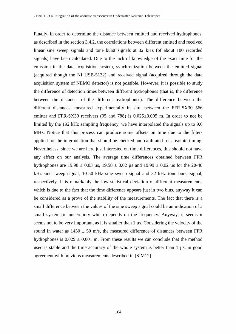
CHAPTER 4. Integration of the acoustic transceiver in Underwater Neutrino Telescopes
104
Finally, in order to determine the distance between emitted and received hydrophones,
as described in the section 3.4.2, the correlations between different emitted and received
linear sine sweep signals and tone burst signals at 32 kHz (of about 100 recorded
signals) have been calculated. Due to the lack of knowledge of the exact time for the
emission in the data acquisition system, synchronization between the emitted signal
(acquired though the NI USB-5132) and received signal (acquired through the data
acquisition system of NEMO detector) is not possible. However, it is possible to study
the difference of detection times between different hydrophones (that is, the difference
between the distances of the different hydrophones). The difference between the
different distances, measured experimentally in situ, between the FFR-SX30 566
emitter and FFR-SX30 receivers (05 and 788) is 0.025±0.005 m. In order to not be
limited by the 192 kHz sampling frequency, we have interpolated the signals up to 9.6
MHz. Notice that this process can produce some offsets on time due to the filters
applied for the interpolation that should be checked and calibrated for absolute timing.
Nevertheless, since we are here just interested on time differences, this should not have
any effect on our analysis. The average time differences obtained between FFR
hydrophones are 19.98 ± 0.03 µs, 19.58 ± 0.02 µs and 19.99 ± 0.02 µs for the 20-40
kHz sine sweep signal, 10-50 kHz sine sweep signal and 32 kHz tone burst signal,
respectively. It is remarkably the low statistical deviation of different measurements,
which is due to the fact that the time difference appears just in two bins, anyway it can
be considered as a prove of the stability of the measurements. The fact that there is a
small difference between the values of the sine sweep signal could be an indication of a
small systematic uncertainty which depends on the frequency. Anyway, it seems it
seems not to be very important, as it is smaller than 1 µs. Considering the velocity of the
sound in water as 1450 ± 50 m/s, the measured difference of distances between FFR
hydrophones is 0.029 ± 0.001 m. From these results we can conclude that the method
used is stable and the time accuracy of the whole system is better than 1 µs, in good
agreement with previous measurements described in [SIM12].
CONCLUSIONS.
105
Conclusions
The main aim of the thesis has been the design, development and test of the acoustic
transceiver for the APS in underwater neutrino telescopes, particularly KM3NeT. The
APS in an underwater neutrino telescope has a double objective: during the deployment
phase, the APS must provide the position of telescope’s mechanical structures, in a geo-
referenced coordinate system, with an accuracy of about 1 m; during the telescope
operation phase, the APS data are used to recover the positions of OMs, which can have
some motion due to the sea currents. Their positions are monitored during the time with
an accuracy of about 10 cm. Then, the R&D activity described in this thesis has been
carried out in order to satisfy these requirements about the acoustic transceiver and APS
in the frame of the KM3NeT Consortium.
The studies realized in order to use the FFR-SX30 transducers as emitters and receivers
in the APS of KM3NeT neutrino telescope (Chapter 3), demonstrated that sensors can
be handled without major problems for the application as transceivers for the KM3NeT
APS, although the variations in power transmission and sensitivity to different
frequencies and angles have to be considered. The intrinsic electronic noise of the FFR-
SX30 hydrophones as receivers is low, but, in case of willing to use the FFR-SX30 as
receiver hydrophones of the KM3NeT APS, a good parameterisation of the sensitivity
as a function of the frequency and angle for each transducer will be needed, especially if
willing to use these hydrophones for deep-sea acoustic monitoring studies or for the
acoustic detection of Ultra-High-Energy neutrinos. For this application, it would be
good to have precise measurements of the sensitivities at larger distances between both
transducers. In fact, some work is going on in this sense within the research group.
Tests in hyperbaric tank have permitted us to conclude that these transducers are quite
stable with depth and the little variations observed are not problematic for the
application.
In order to integrate the transceiver prototype (FFR-SX30 plus SEB) in the
instrumentation line of the ANTARES neutrino telescope and in the NEMO Phase II
tower for the in situ tests in deep-sea, it has been tested in a fresh-water tank in the
laboratory, in a pool and in shallow sea water. For simplicity and due to limitations to
both infrastructures, it was decided to test the transceiver only as emitter. The receiver
CONCLUSIONS.
106
functionality will be tested in other in situ KM3NeT tests. The changes performed in the
transceiver, particularly in the SEB, show the capacity to adapt the electronic parts to
the situation and available conditions.
The transceiver prototype, with low power consumption, is able to have a transmitting
power above 170 dB re 1µPa @ 1 m in agreement with the electronics design and the
specifications needed. It may be considered low in comparison with the ones used in
Long Base Line positioning systems, which usually reach values of 180 dB re 1µPa @ 1
m. Despite this, the use of wideband signals, Maximum Length Sequence (MLS) signals
and sine sweep signals, instead of pure sinusoidal signals result to be in an improvement
of the signal-to-noise ratio, and therefore resulting in an increase in the detection
efficiency, as well as in the accuracy of the time of detection. In this way, tests in fresh-
water pool and in Gandia Harbour have permitted us to say that the accuracy is better
than 30 µs and compatible with uncertainties on the order of a microsecond measured
previously in the laboratory.
The system tested has been finally integrated in the active anchor of the Instrumentation
Line of ANTARES together with the Laser Beacon used for timing calibration
purposes. The expected pressure level and the expected electric signal for the
AMADEUS and some ANTARES hydrophones have been calculated. The use of the
transceiver prototype in combination with the AMADEUS hydrophones makes the test
very complete since it allows studying the transceiver emission for different conditions
of distances and orientation. Moreover, it is possible to study in situ different kinds of
signals and their performance for positioning purposes.
The system for the NEMO Phase II tower base is already available and will be
integrated in May this year. Tests in a water pool at IDASC in Rome have allowed us to
evaluate and compare the performances of the two hydrophone models, SMID and FFR-
SX30 for the integration in NEMO tower. The intrinsic electronic noise and the
receiving voltage response have been measured. Moreover, tests on the prototype
transceiver (FFR-SX30 plus SEB) with the whole data acquisition system of the NEMO
detector have been done showing the compatibility and functionality of both system and
a time of accuracy for the detection better than 1 µs. Also in this case the expected
pressure and electric signal on the receiver hydrophones for an emitted signal of 30 kHz
have been calculated. The results show that the signal level is enough to be recorded.

CONCLUSIONS.
107
Finally, we would like to remark that the acoustic system proposed is compatible with
the different options for the receiver hydrophones proposed for KM3NeT and it is
versatile, so in addition to the positioning functionality, it can be used for acoustic
detection of neutrinos studies or for acoustic monitoring studies in deep-sea. Moreover,
the transceiver (with slight modifications) may be used in other marine positioning
systems, alone or combined with other marine systems, or integrated in different Earth-
Sea Observatories, where the localization of the sensors is an issue. In that sense, the
experience gained from this research can be of great use for other possible applications.

108

ACRONYMS.
109
Acronyms
ACOU: Acoustic Board ADC
ADCPs: Acoustic Doppler Current Profilers
ADC: Analog-to-Digital Converter
AMADEUS: Antares Modules for Acoustic DEtection Under the Sea
AMANDA: Antartic Muon And Neutrino Detector Array
AM: Acoustic Module
ANTARES: Astronomy with a Neutrino Telescope and Abyss environmental RESearch
ANTARES DAQ: ANTARES Data Acquisition
ASDIC: Allied Submarine Detection Investigation Committee
APS: Acoustic Positioning System
AWG: American Wire Gauge
BSS: Bottom string Socket
CDR: Conceptual Design Report
CNRS: Centre national de la recherche scientifique
CPPM: Centre de physique des particules de Marseille
CRC: Cyclic Redundancy Check
CTD: Conductivity – Temperature - Depth
DGPS: Differential GPS
DOM: Digital Optical Module
DU: Detection Unit
DWDM: Dense Wavelength Division Multiplexed
ECAP: Erlangen Centre for Astroparticle Physics
EFCM: Earth Floor Control Module
ACRONYMS.
110
FFR: Free Flooded Ring
FCM: Floor Control Module
GPS: Global Positioning System
HFLBL: High Frequency Long Baseline positioning system
IceCube: Ice Cubic kilometer south pole neutrino observatory
IDASC: Istituto di Acustica e Sensoristica “Orso Mario Corbino”
IFREMER: Institut Français de Recherche pour L’exploitation de la Mer
IL: Instrumentation Line
INFN: Istituto Nazionale di Fisica Nucelare
JB: Junction Box
KM3NeT: km3 Neutrino Telescope
LB: Laser Beacon
LBL: Long Base Line
LCM: Local Control Module
LFLBL: Low Frequency Long Baseline positioning system
LVDS: Low-Voltage Differential Signaling
MLS: Maximum Length Sequence
NEMO: Neutino Mediterranean Observatory
NESTOR: Neutrino Extendend Submarine Telescope with Oceanographic Research
OM: Optical Module
PMT: Photomultiplier
PPM: Pre-Production Model
PPS: Pulse Per Second
PVDF: polyvinylidene bifluoride
PWM: Pulse Width Modulation
PZT: Lead Zirconate Titanate (piezoelectric ceramic material)

ACRONYMS.
111
R&D: Research and Development
ROV: Remotely Operating Vehicle
RVR: Receiving Voltage Response
Rx: Receiver
RxTx: Transceiver
SEB: Sound Emission Board
SBLs: Short-Baseline systems
SMID: Security Multi-Sensor Integrated Devices
SONAR: SOund NAvigation and Ranging
TCM2: Electronic Tilt-Compass sensor Module
TCS: Tiltmeter-Compass System
TDR: Technical Design Report
TDoA: Time Difference of Arrival
TOA: Time of Arrival
TOE: Time of Emission
TOF: Time of Flight
TPE: Thermoplastic elastomer
TSSC: Time Spectral Spread Codes
TVR: Transmitting Voltage Response
USBLs: Ultra-Short-Baseline systems
UPV: Universitat Politècnica de València

112

REFERENCES.
113
References
[ACSAw] ACSA homepage, available on: <http://www.underwater-gps.com>.
[ARD09] M. Ardid (for the ANTARES Collaboration), Positioning system of the
ANTARES neutrino telescope, Nucl. Instr. and Meth. A 602 (2009) 174-176.
[ADR11] S. Adrian Martinez et al., ANTARES Collaboration, First search for point
sources of high energy cosmic neutrinos with the ANTARES neutrino telescope,
Astrophys. J. Lett. 743 (2011) L14-L19.
[ADR12] S. Adrian Martinez et al., ANTARES Collaboration, The Positioning System
of the ANTARES Neutrino Telescope, arXiv:1202.3894v1 [astro-ph.IM].
[AGE11] M. Ageron et al., ANTARES Collaboration, ANTARES: The first undersea
neutrino telescope, Nucl. Instr. and Meth. A 656 (2011) 11-38.
[AGILw] AGILENT Technologies homepage, available on:
<http://www.home.agilent.com/>.
[AGU05] J. A. Aguilar et al., ANTARES Collaboration, Study of large hemispherical
photomultiplier tubes for the ANTARES neutrino telescope, Nucl. Instr. and Meth. A
555 (2005) 132-141.
[AGU11] J. A. Aguilar et al., ANTARES Collaboration, Time calibration of the
ANTARES neutrino telescope, Astroparticle Physics, 34 (2011), 539-549.
[AGU11a] J.A. Aguilar et al. (ANTARES Collaboration), AMADEUS—The acoustic
neutrino detection test system of the ANTARES deep-sea neutrino telescope,Nucl. Instr.
and Meth. A 626–627 (2011) 128.
REFERENCES.
114
[AGU11b] J.A. Aguilar et al., ANTARES Collaboration, Search for a diffuse flux of
high-energy vµ with the ANTARES neutrino telescope Phys. Lett. B 696 (2011) 16-22.
[AMO08] I. Amore, Ph.D. thesis, University of Catania, 2008.
[AMO09] Isabella Amore, NEMO Collaboration, First results from the NEMO Phase-1
experiment, Nucl. Instr. and Meth. in Phys. Res. A 602 (2009) 68–71.
[ANTAw] ANTARES homepage, available on: <http://antares.in2p3.fr>.
[ARD09] M. Ardid, ANTARES Collaboration, Positioning system of the ANTARES
neutrino telescope, Nucl. Instr. and Meth. A, Volume 602, (2009), pp. 174-176.
[ARD10] Ardid, M, M.Bou-Cabo, F.Camarena, V.Espinosa, G.Larosa, C.D.Llorens,
J.A.Martínez-Mora, (For the KM3NeT Consortium), A prototype for the acoustic
triangulation system of the KM3NeT deep sea neutrino telescope. Nucl. Instr. and
Meth. A, 617 (2010) 459-461.
[AYN06] V. Aynutdinov et al., Baikal Collaboration, The Baikal neutrino telescope,
Nucl. Instr. and Meth. in Phys. Res. A 567 (2006) 423.
[BAR01] M. Barr, Introduction to Pulse Width Modulation, Embedded Systems
Programming 14 No. 10, 2001,p. 103.
[BIG09] Ciro Bigongiari, The KM3NeT project for a Very Large Submarine Neutrino
Telescope, Ad Hoc & Sensor Wireless Networks, Old City Publishing, Inc, 00, (2009)
1–22.
[BRO09] A.M. Brown, ANTARES Collaboration, Positioning system of the ANTARES
Neutrino Telescope, proceedings of the 31st ICRC, LÓDZ 2009, arXiv:0908.0814v1
[astro-ph.IM].

REFERENCES.
115
[BRU10] J. Brunner, ANTARES Collaboration , The ANTARES neutrino telescope:
status and first results, Nucl. Instr. and Meth. A, 626-627 (2010) S19-S24.
[CDR08] KM3NeT Conceptual Design Report (2008) ISBN 978-90-6488-031-5,
available on: <www.km3net.org>.
[CHE77] Chen and Millero, Speed of sound in seawater at high pressures, J. Acoust.
Soc. Am., Vol. 62, No. 5, 1129-1135, Nov. 1977.
[DAV02] Fundamentals and Applications of ULTRASONIC WAVES, J. David N.
Cheeke, CRC Press LLC, 2002.
[ECAw] ECA homepage, available on: < http://www.eca.fr>.
[FALCw] FALCO Systems homepage, available on: <http://www.falco-systems.com/>.
[FRA82] R. E. Francois and G. R. Garrison, Sound absorption based on ocean
measurements: Part I: Pure water and magnesium sulfate contributions, J. Acoust. Soc.
Am. Volume 72, Issue 3, (1982), pp. 896-907.
[HUL11] K. Hultqvist, IceCube Collaboration, IceCube: physics, status and future,
Nucl. Instr. and Meth. A, 626-627 (2011) S6-S12.
[IDASw] Istituto di Acustica e Sensoristica “Orso Mario Corbino” homepage, available
on: <http://www.idasc.cnr.it/>.
[IFREw] IFREMER homepage, available on: <http://www.ifremer.fr>.
[ISELw] ISEL automation homepage, available on: <http://www.isel-germany.de/>.
[ITCw] ITC-Transducers home page, available on: <http://www.itc-transducers.com>.
[IXSEw] IXSEA homepage, available on: < www.ixsea.com>.
REFERENCES.
116
[KEL07] P. Keller, Acoustic Positioning System for the Deep-Sea ANTARES Neutrino
Telescope, Proc. SENSORCOMM Conf., 2007, 243-247 – ISBN: 0-7695-2988-7.
[KAL11] O. Kalekin, J.J.M.Steijger, H.P.Peek, (For the KM3NeT Collaboration),
Photomultipliers for the KM3NeT optical modules, Nucl. Instr. and Meth. A in press,
proceeding of the New Developments In Photodetection (NDIP) congress 2011, DOI:
10.1016/j.nima.2011.11.004.
[KAT11] U.F. Katz, (For the KM3NeT Collaboration), The KM3NeT project, Nucl.
Instr. and Meth. A, 626-627 (2011) S57-S63.
[KM3Nw] KM3NeT homepage, available on: <http://www.km3net.org>.
[LAH12] R. Lahamann, (For the ANTARES Collaboration), Status and recent results of
the acoustic neutrino detection test system AMADEUS, Nucl. Instr. and Meth. A 662
(2012) S216-S221.
[LAR12] G. Larosa, M. Ardid, C. D. Llorens, M. Bou-Cabo, J. A. Martínez-Mora, S.
Adrían-Martínez, Development of an Acoustic Transceiver for Positioning Systems in
Underwater Neutrino Telescopes, IARIA, proceeding of the GEOProcessing2012
congress, ISBN: 978-1-61208-178-6, 2012.
[LAR12a] Larosa, G; et al. Development of an acoustic transceiver for the KM3NeT
positioning system, Nucl. Instr. Meth. A 2012, accepted.
[LLO12] C.D. Llorens et al., The Sound Emission Board of the KM3NeT Acoustic
Positioning System, J. Instrum. (2012), 7, C01001.
[LUR02] An Introduction to Underwater Acoustics: Principles and Applications,
Xavier Lurton, Springer, Praxis Publishing Ltd, Chichester, UK, 2002.

REFERENCES.
117
[McArw] McArtney-EurOceanique SAS homepage, available on:
<http://www.macartney.com>.
[MICOw] MICOS (Mechanische Instrumente Optische Systeme GMBH) homepage,
available on: <www.micos.ws>.
[MICRw] Microchip homepage, available on: <http://www.microchip.com>.
[MIG06] E. Migneco, et al., Status of NEMO, Nucl. Instr. and Meth. A 567 (2006) 444-
451.
[MODBw] MODBUS homepage, available on:
<http://modbus.org/docs/Modbus_Application_Protocol_V1_1b.pdf>
[NATIw] National Instruments homepage, available on: <http://www.ni.com>.
[NEMOw] NEMO homepage, available on: <http://nemoweb.lns.infn.it>.
[NESTw] NESTOR homepage, available on: < http://www.nestor.org.gr>.
[MAR06] A. Margiotta, NEMO Collaboration, Status report of the NEMO (Neutrino
Mediterranean Observatory) project, Phys. Scr. T127 (2006) 107–108.
[MED05] Sounds in the sea: From Ocean Acoustics to Acoustical Oceanography,
Herman Medwin and colleagues, Cambridge University Press, 2005.
[PNICw] PNI Sensor Corporation homepage, available on: <http://www.pnicorp.com>.
[RESOw] RESON homepage available on: <http://www.reson.com>.
[RIC04] G. Riccobene, L. Cosentino, M. Musumeci, G. Pavan, F. Speziale, Acoustic
detection of UHE neutrinos: a station for measurement of the deep sea acoustic noise,
Nucl. Instr. and Meth. A, 518 (2004) 220–222.
REFERENCES.
118
[RIC09] G. Riccobene, NEMO Collaboration, Long-term measurements of acoustic
background noise in very deep sea, Nucl. Instr. and Meth. A, 604 (2009) S149–S157.
[SEACw] SEACON homepage, available on: <http://seaconworldwide.com>.
[SENSw] Sensorthech homepage, available on: <http://www.sensortech.ca>.
[SHE07] C.H. Sherman and J.L. Butler, Transducers and Array for Underwater Sound,
The Underwater Acoustic Series, Springer, 2007.
[SIM11] F. Simeone, S. Viola, The SMO project: a submarine multidisciplinary
observatory in deep-sea, MASS, pp.898-903, 2011 IEEE Eighth International
Conference on Mobile Ad-Hoc and Sensor Systems, (2011). ISBN: 978-076954469-4;
DOI 10.1109/MASS.2011.107.
[SIM12] F. Simeone, F. Ameli, M. Ardid, V. Bertin, M. Bonori, M. Bou-Cabo, C. Calì,
A. D’Amico, G. Giovanetti, M. Imbesi, P. Keller, G. Larosa, C.D. Llorens, R. Masullo,
N. Randazzo, G. Riccobene, F. Speziale and S. Viola, KM3NeT consortium, Design
and first tests of an acoustic positioning and detection system for KM3NeT, Nucl. Instr.
and Meth. A, 662 (2012) S246-S248.
[SMIDw] SMID Technology homepage, available on: <http://www.smidtechnology.it>.
[SPI05] Ch. Spriering, Neutrino Astrophysics in the Cold: Amanda, Baikal and
IceCube,Phys. Scripta T121 (2005) 112-118.
[TDR11] KM3NeT Technical Design Report (2011) ISBN 978-90-6488-033-9,
available on: <www.km3net.org>.
[VIO12] S. Viola, NEMO and SMO Collaborations, M. Ardid, V. Bertin, A.
Enzenhöfer, V. Espinosa, P. Keller, R. Lahmann, G. Larosa, C.D. Llorens, NEMO-SMO
acoustic array: a deep-sea test of a novel acoustic positioning system for a km3-scale
underwater neutrino telescope, Nucl. Instr. and Meth. A, (2012) accepted.

ACKNOWLEDGMENTS.
119
Acknowledgments
I am sincerely grateful for the help of Dr. Miguel Ardid who gave me the opportunity to
obtain my PhD in Spain by working with KM3NeT and ANTARES collaborations.
Also I would like to thank him and all members of the Gandia group for assisting me in
enhancing my knowledge in underwater acoustics, during these last four years.
Likewise, the reviewers of my thesis Dr. J, Zornoza, Dr. R. Lahmann and Dr. G.
Riccobene shall be mentioned as their constructive comments have contributed to the
improvement of my thesis.
Special gratitude is expressed to my family for their emotional support and
unconditional love; in particular I want to thank Demetrio for his love and patience
during our time together and especially in these hard years.
Moreover, this work has been supported by the Ministerio de Ciencia e Innovación
(Spanish Government), project references FPA2009-13983-C02-02, ACI2009-1067,
AIC10-D-00583, Consolider-Ingenio Multidark (CSD2009-00064). It has also been
funded by Generalitat Valenciana, Prometeo/2009/26, and the European 6th and 7th
Framework Programme, contract no. DS 011937 and grant no. 212525.