Graduate Theses, Dissertations, and Problem Reports

2018

DESIGN AND DEVELOPMENT OF TEST RIGS TO DESIGN AND DEVELOPMENT OF TEST RIGS TO

EXPERIMENTALLY INVESTIGATE FLOW LOSS AND HEAT EXPERIMENTALLY INVESTIGATE FLOW LOSS AND HEAT

TRANSFER IN A STIRLING ENGINE HEATER HEAD TRANSFER IN A STIRLING ENGINE HEATER HEAD

Pawan K. Yadav

Follow this and additional works at: https://researchrepository.wvu.edu/etd

Part of the Heat Transfer, Combustion Commons

Recommended Citation Recommended Citation Yadav, Pawan K., "DESIGN AND DEVELOPMENT OF TEST RIGS TO EXPERIMENTALLY INVESTIGATE FLOW LOSS AND HEAT TRANSFER IN A STIRLING ENGINE HEATER HEAD" (2018). Graduate Theses, Dissertations, and Problem Reports. 7492. https://researchrepository.wvu.edu/etd/7492

This Thesis is protected by copyright and/or related rights. It has been brought to you by the The Research Repository @ WVU with permission from the rights-holder(s). You are free to use this Thesis in any way that is permitted by the copyright and related rights legislation that applies to your use. For other uses you must obtain permission from the rights-holder(s) directly, unless additional rights are indicated by a Creative Commons license in the record and/ or on the work itself. This Thesis has been accepted for inclusion in WVU Graduate Theses, Dissertations, and Problem Reports collection by an authorized administrator of The Research Repository @ WVU. For more information, please contact researchrepository@mail.wvu.edu.

DESIGN AND DEVELOPMENT OF TEST RIGS TO EXPERIMENTALLY INVESTIGATE FLOW LOSS AND HEAT TRANSFER IN A

STIRLING ENGINE HEATER HEAD

Pawan Kumar Yadav

Thesis submitted to the Benjamin M. Statler College of Engineering and Mineral Resources

at West Virginia University

in partial fulfillment of the requirements for the degree of

Master of Science in Mechanical Engineering

Songgang Qiu, Ph.D., Chair V’yacheslav Akkerman, Ph.D.

Hailin Li, Ph.D.

Department of Mechanical and Aerospace Engineering

Morgantown, West Virginia 2018

Keywords: Stirling Engine, Heater Head, Fluid, Pressure Drop, Heat Transfer, CHP

Copyright 2018 Pawan Kumar Yadav

Abstract

DESIGN AND DEVELOPMENT OF TEST RIGS TO EXPERIMENTALLY INVESTIGATE FLOW LOSS AND HEAT TRANSFER IN A

STIRLING ENGINE HEATER HEAD

Pawan Kumar Yadav

The Stirling engines are attractive alternative for combined heat and power (CHP) systems, especially for high efficiency power generation using different heat sources. The hot side heat exchanger or heater head (HH) is one of the indispensable components of Stirling engines which transfers the heat from outside of the system into the working fluid. For development of a low cost, highly efficient and reliable CHP system, a novel HH has been designed and additively manufactured from Inconel 625.

For the investigation of flow loss and heat transfer through this Stirling engine heater head, two benchtop test rigs were designed, developed, and manufactured. One rig is to evaluate flow loss in oscillating flow conditions (called flow loss test rig- FLTR) and another is to evaluate heat transfer in unidirectional flow conditions (called heat transfer test rig- HTTR). For the FLTR, a linear actuator from Parker is used to generate and maintain the oscillating flow by driving a piston in oscillatory motion. The rod and the piston are sealed against the working fluid leakage using Trelleborg seals. At room temperature, by varying the charge pressure, frequency, and stroke length, multiple test conditions were achieved for experimentation. For the HTTR, a Gast’s high-flow, low-pressure compressed air blower is used to deliver the unidirectional flow. The data acquisition (DAQ) is comprised of National Instruments’ cDAQ and modules to measure piston’s motion in real time and dynamic pressure with Kistler’s pressure transducers.

Presented also are the detailed testing procedures, some preliminary results, expected results from Sage, and discussion of computational fluid dynamics (CFD) outputs that were used to check against the experimentally measured data from the FLTR. Preliminary results from FLTR showed higher pressure drop across the heater head tubes when compared to the Sage and CFD predictions, and higher coefficient of friction (Cf) when compared to Sage.

iii

DEDICATION

This thesis and all my academic achievements are dedicated to my parents:

Mr. Ramashankar Prasad Yadav and Mrs. Kishuni Devi Yadav

iv

ACKNOWLEDGEMENTS

I am profoundly grateful to my advisor, Professor Songgang Qiu, for giving me the opportunity to

work in his group at Stirling Engine Laboratory. This research would have been impossible without

his guidance, inspiration, and support. I would also like to thank my thesis committee,

Dr. V’yacheslav Akkerman and Dr. Hailin Li for their insightful comments and suggestions.

I have my deepest appreciation to my beloved parents, my sister Renu Yadav, my brother-in-

law Harendra Ray Yadav, and to all my family members and to my friends in Nepal and here in the

USA. I am very grateful for being blessed with them to have by my side in this endeavor, for their

continuous love, support, and encouragement.

My sincere thanks go to my fellow labmates: Koji Yanaga- for the fruitful discussions that we

have had and his useful suggestions, especially with the data processing and LabVIEW coding;

Dr. Laura Solomon- for her valuable ideas on troubleshooting the experimental conditions, results

analyses, and with the CFD data; Dr. Yuan Gao- for the updated CAD models of heater head

system, every time the Sage model was updated, for getting the heater head additively

manufactured for my experimentation, and also for the discussions and drawings on heater design;

and Garrett Rinker- for helping me with the Finite Element Analysis (FEA).

Heartfelt thanks go to Amanda DuPont and Kelsey Crawford, including all the staff at the

Department of Mechanical and Aerospace Engineering at West Virginia University (WVU), who

have directly or indirectly assisted me with this research and my time at WVU. Last but not the

least, I am also thankful to Dan Davis from Wilson Works for manufacturing the components of the

test rigs.

v

Table of Contents Abstract ................................................................................................... ii

Dedication .............................................................................................. iii

Acknowledgments .................................................................................. iv

Table of Contents……………………………………………………………v

LIST OF FIGURES ............................................................................... vii

LIST OF TABLES .................................................................................. ix

LIST OF SYMBOLS / NOMENCLATURE .............................................. x

1. INTRODUCTION ................................................................................ 1

1.1 Stirling Engine………………………………………………….1

1.2 Project at WVU………..……………………………………….5

1.3 Motivation for this study ………………………………………7

1.4 Literature Review ……………………………………………...9

2. EXPERIMENTAL STUDY………………………………………………12

2.1 Description of Test Rigs………………………………….….12

2.2 Mechanical Testing of the Heater Head…………………….26

2.3 Procedure………………………………………………………27

3. DATA ACQUISITION AND PROCESSING...…………………………30

3.1 Collecting data from pressure transducer…………………...30

3.2 Collecting piston's position data……………………………...30

3.3 Synchronization of position and pressure data……………..31

vi

3.4 Data Processing………………………………..…………….32

4. RESULTS AND DISCUSSION.……………………………………….34

4.1 Preliminary Results...………………………………………..37

4.2 Sage and CFD comparision...………………………………40

4.3 Uncertainty Analysis…………………………………………42

5. CONCLUSIONS………………………………………………………..45

5.1 Future Works……………………………….………………...46

6. REFERENCES ................................................................................. 47

7. APPENDIX……………………………………………………………....51

vii

LIST OF FIGURES

Figure 1- Different configurations of Stirling Engine- (a) Alpha, (b) Beta and (c) Gamma [5]……...2

Figure 2- Free-piston Stirling engine [7]…………………………………………………………………...3

Figure 3- A Pressure vs. Volume graph of the Idealized Stirling Engine [1]………………………..….4

Figure 4- Different types of Stirling engine heater head configurations. (a) Monolithic, (b) Flat

tubular, and (c) Vertical tubular………………………………………………………………….8

Figure 5- (a) Flow guides and tube bundle of Tubular heater head and (b) Layout of Tubular heater

head tubes…………………………………………………………………………………………8

Figure 6- Heater Head ISO View (left) and additively manufactured Heater Head (right)……………9

Figure 7- Schematics of FLTR (left) and HTTR (right)………………………………………………….12

Figure 8- Benchtop flow loss test rig- CAD Model………………………………………………………13

Figure 9- Benchtop flow loss test rig complete assembly with actual hardware……………………..13

Figure 10- Thermal boundary condition for the Cylinder………………………………………………..15

Figure 11- Structural boundary conditions for the Cylinder…………………………………………….15

Figure 12- Steady-State Thermal analysis of the Cylinder……………………………………………..16

Figure 13- Static Structural analysis of the Cylinder…………………………………………………….16

Figure 14- Structural boundary conditions for the End Plug……………………………………………17

Figure 15- Static Structural analysis of the End Plug…………………………………………………...17

Figure 16- Structural boundary conditions for the Elbow……………………………………………….18

Figure 17- Static Structural analysis of the Elbow………………………………………………………18

Figure 18- Structural boundary conditions for the Buffer Volume……………………………………...19

Figure 19- Static Structural analysis of the Buffer Volume……………………………………………..19

Figure 20- Parker’s Linear Actuator and IPA drive controller…………………………………………..21

Figure 21- Manufactured piston and cylinder models…………………………………………………..21

Figure 22- (a) Additively manufactured Regenerator (b) Heat rejecter………………………………..22

Figure 23- Balance system to ensure linear actuator and the piston-cylinder are well aligned…….23

Figure 24- CAD model of the Heat Transfer Test Rig…………………………………………………..24

Figure 25- Air Blower for the Heat Transfer Test Rig…………………………………………………...24

Figure 26- Schematic of the Heater Design……………………………………………………………..25

Figure 27- Layout of the Heater Design………………………………………………………………….25

Figure 28- Pressure and leak proof test of additively manufactured Heater Head…………………..26

Figure 29- Illustration of the oscillating flow in FLTR …………………………………………………...29

Figure 30- Illustration of the unidirectional flow in HTTR……………………………………………….29

viii

Figure 31- National Instruments’ cDAQ 9178 and modules NI 9234, NI 9213, and NI 9411 (from left

to right)…………………………………………………………………………………………31

Figure 32- Flow in the heater head, going from right to left…………………………………………….36 Figure 33- Flow in the heater head, going from left to right…………………………………………….36

Figure 34- Ensemble-averaged position, velocity, and pressure drop at 3 Hz, 13.4 mm amplitude,

and 700000 Pa absolute……………………………………………………………………..38

Figure 35- Ensemble-averaged pressure at sensor 1, sensor 2, and pressure drop at 3 Hz, 13.4 mm

amplitude, and 700000 Pa absolute………………………………...………………………38

Figure 36- Ensemble-averaged pressure at sensor 1 at 13.4 mm amplitude, and 700000 Pa

absolute, curve fitted to Sine wave in MATLAB…………………………………………....39

Figure 37- Ensemble-averaged pressure at sensor 2 at 13.4 mm amplitude, and 700000 Pa

absolute, curve fitted to Sine wave in MATLAB……………………………………………39

Figure 38- Pressure drop- experimental and CFD, vs time for a cycle at 3 Hz, 13.4 mm amplitude,

and 700000 Pa absolute……………………………………………………………………..40

Figure 39- Ensemble-averaged pressure drop from CFD vs. the ensemble-averaged pressure

drop from experiment, for Coefficient of Determination, R2 being 0.9686.….……...……41

Figure 40- Maximum coefficient of friction (Cf-max) versus maximum Reynolds number (Remax) –

comparing Experimental and Theoretical Cf-max at same Remax….….……………………42

Figure 41- Comparison of pressure drop for 6 different experiments with 6 different Reynolds

number, for experimental case and 3 different friction factor correlations….……………43

Figure 42- Ensemble-averaged position, velocity, and pressure drop at 3 Hz, 13.4 mm amplitude,

and 700000 Pa absolute, over 5 experiments at same operating conditions…………...46

Figure 43- Ensemble-averaged pressure drop for an experiment and for over 5 experiments at

same operating conditions, at 3 Hz, 13.4 mm amplitude, and 700000 Pa absolute……46

Figure 44- Coefficient of Variation of 11 experimental pressure drop data, plotted against the time

for a cycle………………………………………………………………………………………47

Figure 45- Coefficient of Variation of 11 experimental pressure drop data, plotted against the

ensemble-averaged pressure drop............…………………………………………………47

ix

LIST OF TABLES

Table 1- Results of Stirling Engine Design from Sage Model [8]………………………………………6

Table 2- Maximum stress, yield stress, and the safety factors for the designed components……...20

Table 3- The Trelleborg’s seals [28]………………………………………………………………………21

Table 4- Variation of linear actuator’s average number of output points per cycle, with frequency,

piston’s amplitude and system’s charged pressure………………………………………….32

Table 5- Expected results for regenerator as predicted by Sage……………………………………...34

Table 6- The minor loss coefficients (Ks) for the heater head tube [32]………………………………36

Table 7- Expected experimental results from HTTR based on Sage [34]…………………………….44

Table 8- The uncertainty in the maximum and minimum pressure drop……………………………...45

x

LIST OF SYMBOLS / NOMENCLATURE

CFD = computational fluid dynamics a = acceleration (m/s2) Atube = area of the tube (m2) Cf = coefficient of friction CAD = computer aided-design CFD = computational fluid dynamics CHP = combined heat and power DAQ = data acquisition Dtube = internal diameter of a tube (m) fr = frequency (Hz) f = friction factor FEA = Finite Element Analysis FLTR = flow loss test rig HTTR = heat transfer test rig HH = heater head Ltube = length of a heater head tube mgas = mass flow rate of gas (kg/s) ppr = pulses per revolution pg = gage pressure (Pa) Δp = pressure drop (Pa) r = internal radius of the pipe (m) Remean = mean Reynolds number Remax = maximum Reynolds number s = stroke length (m) t = thickness of the pipe wall (m) v = velocity (m/s) vpiston = velocity of piston (m/s) vmean-gas = mean velocity of gas (m/s) vmax-gas = maximum velocity of gas (m/s) Va = Valensi number x = distance (m) xp = amplitude (m) ρgas = density of gas (kg/m3) μgas = dynamic viscosity of gas (Pa.s) νgas = kinematic viscosity of gas (m2/s) σ1 = hoop stress (Pa) ω = angular frequency (rad/s)

1

C H A P T E R 1 . I N T R O D U C T I O N

1.1 STIRLING ENGINE

According to the ubiquitous Wikipedia [1], a Stirling engine is closed-cycle regenerative heat engine

with a gaseous working fluid. It operates by cyclic compression and expansion of this fluid at

different temperatures as such there is conversion of heat energy to mechanical work. Here, the

‘closed-cycle’ refers to a thermodynamic system where the working fluid is permanently contained

within the system, and the ‘regenerative’, refers to the use of an internal heat exchanger, which also

acts like thermal storage unit, known as regenerator.

History

A 100 percent Renaissance man, partly preacher, and partly inventor, the Scottish minister Robert

Stirling (1970-1878) invented the Stirling engine. He named it “air engine”- as steam engines of his

days would often explode, but these air engines would not explode, instead would produce more

power than existing steam engines [2]. Patented in 1816, the first practical use of Stirling engine

was in pumping water in a quarry in 1818; the main subject of the patent was a type of heat

exchanger called “economizer”, now generally known as a “regenerator”.

To maximize power and efficiency, Stirling engine needs to operate at very high temperatures

and this became limiting factor because of the materials of those days. In the later nineteenth

century, as steam engines became safer, Stirling engine could not compete with steam engines at

industrial scale power source; this also stagnated the further improvements in the design of the

Stirling engines [1].

With the development of modern materials, toward the mid-twentieth century, interests picked

up in further developing these externally combustible Stirling engines. Unlike the internal

combustion engine with Otto cycle or Diesel cycle, Stirling engines are highly efficient, able to

achieve up to 50% efficiency, in addition of being quiet in operation and adaptable to almost any

heat source. There was an ambitious effort to develop automobile Stirling engines in the USA and

2

Europe from 1950’s through 1980’s, however, this program failed because of significantly high gas

pressure requirement to meet acceptable specific power output [3] .

After spending substantial time and efforts, Phillips had started getting some success around

1970s with “reversed Stirling engine”- cryocoolers. Meanwhile, William Beale founded Sunpower

Inc. (1974), mainly based on his free-piston Stirling engine invention of 1964. With lean method,

added with solid engineering of some brilliant minds, Sunpower invented, perfected, and made the

free piston variant of Stirling engine commercially available throughout the world [4].

Types/Configurations

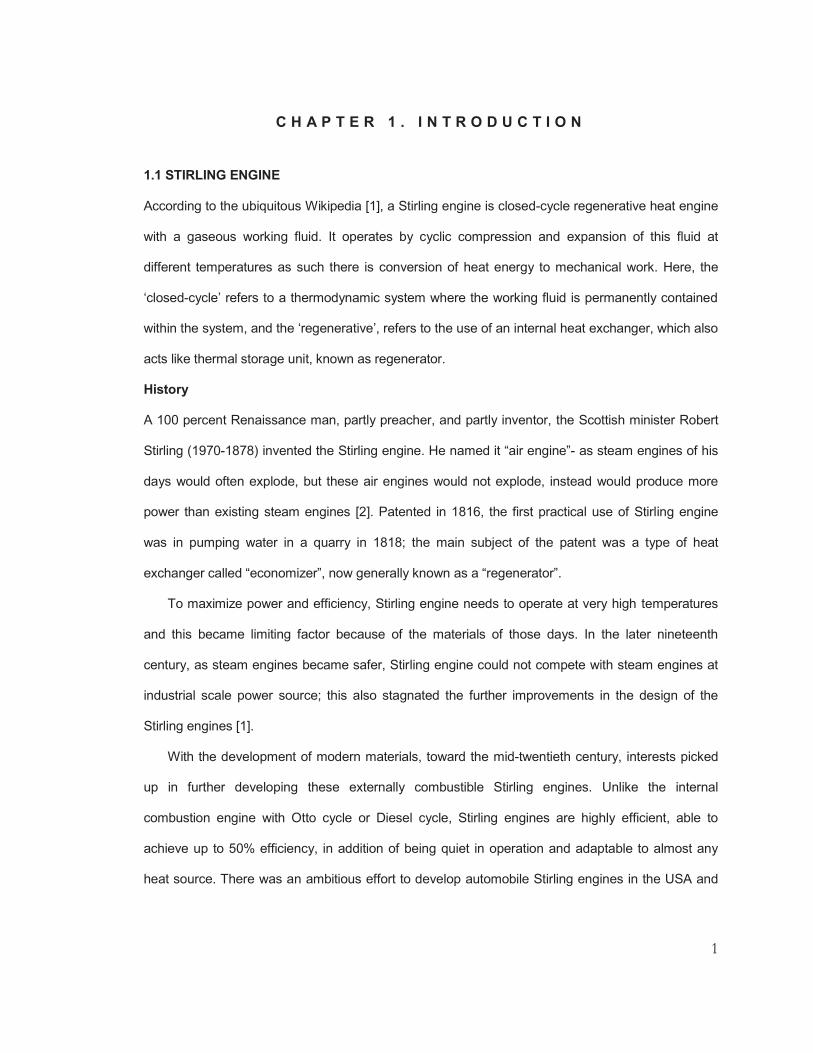
Based on how the working fluid move in between hot and cold space, the Stirling engines can be

categorized in three major configurations- shown in figure 1 [5].

(a) Alpha (b) Beta (c) Gamma

Figure 1: Different configurations of Stirling Engine- (a) Alpha, (b) Beta and (c) Gamma [5]

1. Alpha Configuration: It comprises of two power pistons- one in hot cylinder and one in cold

cylinder, the gas is driven between the two by these pistons.

2. Beta Configuration: A single cylinder configuration with a hot and a cold end, it contains both

power piston and displacer- that drives the gas between hot and cold ends.

3. Gamma Configurations: It has two cylinders, one containing a displacer with a hot and cold end,

and one containing power piston; these two cylinders are joined to form a single space with the

same pressure in both cylinders.

3

Free-piston Stirling engines: Invented and developed by William Beale at Ohio University, Free-

piston Stirling engines are the most ingenious Stirling engines yet invented, main aspect being-

devoid of all mechanical linkage system [6]. Here, the output power can be added or obtained

through linear alternator, pump, or other coaxial device, allowing the entire system to be

hermetically sealed, thereby nearly eliminating all moving parts and associated friction and wear.

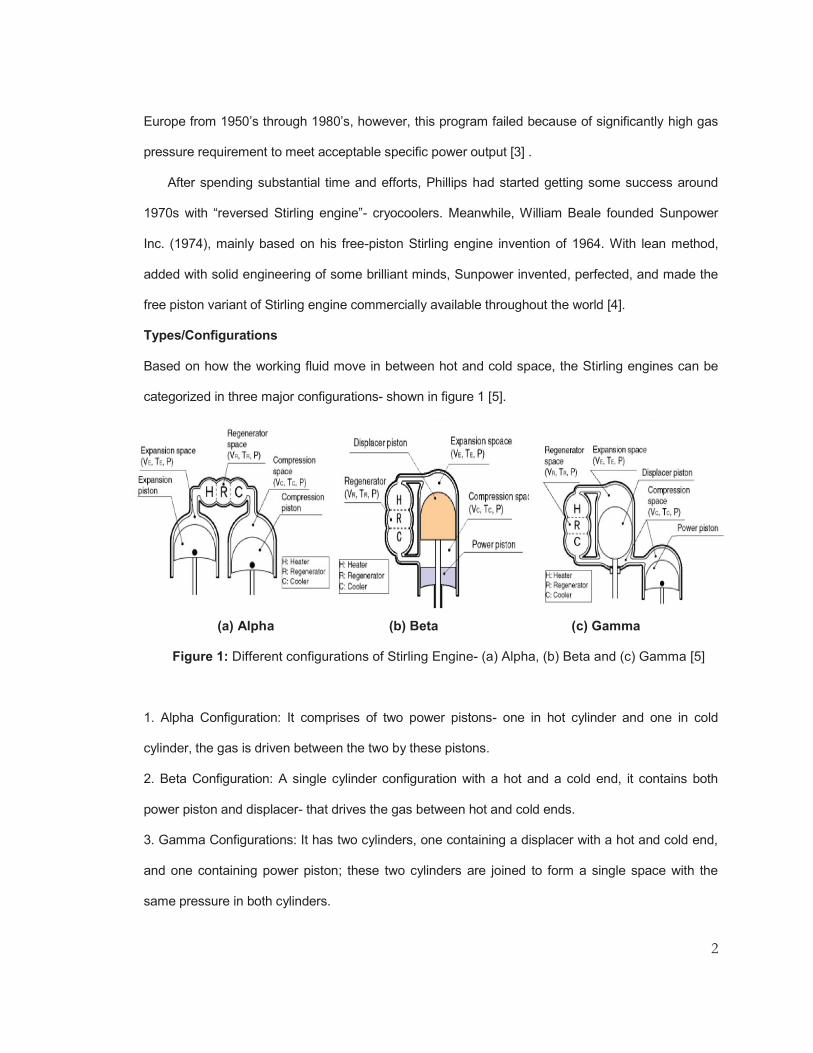
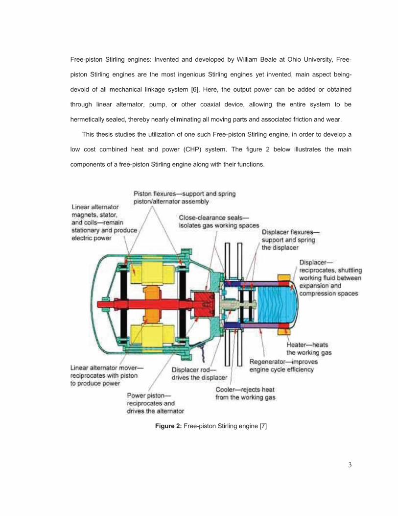
This thesis studies the utilization of one such Free-piston Stirling engine, in order to develop a

low cost combined heat and power (CHP) system. The figure 2 below illustrates the main

components of a free-piston Stirling engine along with their functions.

Figure 2: Free-piston Stirling engine [7]

4

Working Principle

An ideal Stirling engine has four thermodynamic processes that act on the working fluid, explained

below and as can be seen in figure 3.

Figure 3: A Pressure vs. Volume graph of the Idealized Stirling Engine [1]

Curve 1- Isothermal Expansion: At constant high temperature of the expansion space and the

associated heat exchanger, the gas undergoes nearly-isothermal expansion, absorbing heat from

the hot source.

Curve 2- Isochoric Heat-Removal: The hot gas passes through regenerator, leaving behind heat

and cooling down, enters the low temperature zone.

Curve 3- Isothermal Compression: The compression space and its associated heat exchanger are

at constant low temperature and thus gas undergoes near-isothermal compression, thereby

rejecting heat to the cold sink

Curve 4- Isochoric Heat-Addition: The cold gas passes back to regenerator, recovering the heat

stored in the regenerator in process 2, and heating up on its way to the high temperature zone.

Components

Based on the working principle and the closed cycle operation, the heat acquired by the working

fluid of Stirling engine needs to be transmitted to the heat sink, which results in few key

components, which are [1]: Working gas, Heat source, Heater/ Hot side heat exchanger – the main

5

topic of this thesis- is a novel, additively manufactured- tubular hot side heat exchanger, called

Heater Head (HH), Regenerator, Cooler/ Cold side heat exchanger, Heat sink, and Displacer

Advantages [1]

1. Stirling engines can run directly on any available heat source- combustion, solar, geothermal,

nuclear, biological, or waste heat from industrial processes.

2. It uses a single-phase working fluid that maintains an internal pressure close to the design

pressure, meaning for a well-designed system, there is very low risk of explosion.

3. They can be run quietly- without an air supply, can be used in submarines. Because of extreme

flexibility, they can be used as CHP in the winter and as coolers in summer.

Disadvantages [1]

1. Size and Cost issues- Because of high temperatures at hot end, materials with low creep are

required which increases the cost of the engine. Also, to keep the coolant at low temperatures,

dissipation of waste heat get complicated, requiring larger radiators, increasing cost and size.

2. Power and Torque issues: Stirling engines have low specific power, i.e., they are quite large for

the power they produce, especially those that run on small temperature differentials. Stirling

engines need warm up time and thus are used mostly as constant speed engines. Also, during the

shutdown, they take a while to stop.

3. Gas choice issues: The gas used needs to have low heat capacity, as the transferred heat is

proportional to the pressure. Mostly, Helium is used because of its very low heat capacity; air and

nitrogen can be other substitutes including methane and ammonia.

1.2. PROJECT AT WVU

This study is a part of a big project that is undergoing in the Stirling Engine Laboratory at the West

Virginia University. The project is titled “Advanced Stirling Power Generation System for Combined

Heat and Power (ASPGen).” The project has been awarded by United States Department of

Energy’s Advanced Research Projects Agency- Energy (DOE’s ARPA-E) under Generator for

Small Electrical and Thermal Systems (GENSETS) program, award number DE-AR0000864.

6

This project aims to develop a low cost CHP system with increased efficiency and reliability. This

system utilizes the free-piston Stirling power generator. The key components are the hot heat

exchanger (heater head), regenerator, cold heat exchanger (heat rejecter), displacer, flexures,

piston, and linear alternator.

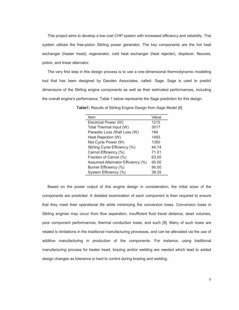
The very first step in this design process is to use a one-dimensional thermodynamic modelling

tool that has been designed by Geoden Associates, called- Sage. Sage is used to predict

dimensions of the Stirling engine components as well as their estimated performances, including

the overall engine’s performance. Table 1 below represents the Sage prediction for this design.

Table1: Results of Stirling Engine Design from Sage Model [8]

Item Value Electrical Power (W) 1215 Total Thermal Input (W) 3017 Parasitic Loss /Wall Loss (W) 184 Heat Rejection (W) 1493 Net Cycle Power (W) 1350 Stirling Cycle Efficiency (%) 44.74 Carnot Efficiency (%) 71.01 Fraction of Carnot (%) 63.00 Assumed Alternator Efficiency (%) 95.00 Burner Efficiency (%) 90.00 System Efficiency (%) 38.25

Based on the power output of this engine design in consideration, the initial sizes of the

components are predicted. A detailed examination of each component is then required to ensure

that they meet their operational life while minimizing the conversion loses. Conversion loses in

Stirling engines may occur from flow separation, insufficient fluid travel distance, dead volumes,

poor component performances, thermal conduction loses, and such [9]. Many of such loses are

related to limitations in the traditional manufacturing processes, and can be alleviated via the use of

additive manufacturing in production of the components. For instance, using traditional

manufacturing process for heater head, brazing and/or welding are needed which lead to added

design changes as tolerance is hard to control during brazing and welding.

7

Considering this, additive manufacturing has been used for manufacturing of key components of

this system, which has reduced the total number of components and thereby the cost. Additionally,

it has also helped in manufacturing complex parts with intricate geometry; such design

improvements to the system has increased its efficiency by reducing dead volumes and associated

flow losses and thermodynamic losses, thereby improving the flow dynamics and heat transfer

characteristics of the components [10, 11].

1.3. MOTIVATION FOR THIS STUDY

This CHP system with a free-piston Stirling engine (FPSE) is for commercial application, with an

estimated life of 30 years and fuel to electric efficiency of more than 40%. The heater head (HH) is

one of the indispensable components of this CHP system, as it impacts the reliability, the lifespan,

and the efficiency of this FPSE. The HH acts like a heat exchanger between the external heat

source and the working fluid of the Stirling engine. With working fluid inside it operating at around

810 ْC and pressure of about 3300000 Pa on the hot end, the hot end is susceptive to creep

deformation; the cold end however, is at low temperature and is not subjected to such creep

deformation. Hence, a balance between thick wall for increased structural creep resistance and thin

wall for optimal heat transfer needs to be reached for an optimal design of this HH [12].

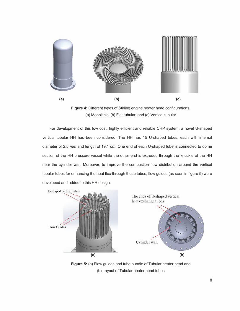
There are three types of HH commonly used in Stirling engines- Monolithic, Flat tubular, and

Vertical tubular HH, these are shown in figure 4. The monolithic HH can be fabricated cheaply, but

due to limited heat flux, it is generally employed for small electrical power convertors. Additionally,

the diameter and length of monolithic HH increases rapidly with increase in power which

dramatically increases the system’s cost and size, and such, it is not suitable for this CHP system.

The flat tubular HH are historically standard for solar Stirling engine applications, and not a good fit

for this CHP system. Eventually, due to large heat exchange surface area and high efficiency of the

U-shaped vertical tubular heat exchanger, Vertical tubular HH was choses for this CHP system [b].

8

(a) (b) (c)

Figure 4: Different types of Stirling engine heater head configurations.

(a) Monolithic, (b) Flat tubular, and (c) Vertical tubular

For development of this low cost, highly efficient and reliable CHP system, a novel U-shaped

vertical tubular HH has been considered. The HH has 15 U-shaped tubes, each with internal

diameter of 2.5 mm and length of 19.1 cm. One end of each U-shaped tube is connected to dome

section of the HH pressure vessel while the other end is extruded through the knuckle of the HH

near the cylinder wall. Moreover, to improve the combustion flow distribution around the vertical

tubular tubes for enhancing the heat flux through these tubes, flow guides (as seen in figure 5) were

developed and added to this HH design.

(a) (b)

Figure 5: (a) Flow guides and tube bundle of Tubular heater head and

(b) Layout of Tubular heater head tubes

9

After a thorough study on heat exchanger selection and analysis, design optimization for dead

volume reduction, axial thermal conduction losses, and stress analysis using Finite Element

Analysis (FEA), the U-shaped tubular HH discussed above was designed and additively

manufactured from Inconel 625, by i3D MFD, as presented in figure 6.

Figure 6: Heater Head ISO View (left) and additively manufactured Heater Head (right)

Thus, the motivation for this thesis was to fully understand and characterize the flow loss and

heat transfer features of this newly designed HH and the HH system (HH, regenerator, and heat

rejecter). In order to do this, experimental test rigs needed to be designed, wherein multiple test

conditions could be run for this purpose.

1.4. LITERATURE REVIEW

For preservation of fossil fuels and reduction of greenhouse effects, there is an increased

desperation to find clean, efficient, and sustainable alternative energy sources such as biomass,

solar, and geothermal. In the field of renewable energy, Stirling engines stand out as they can utilize

10

various renewable energy sources to efficiently generate power [13]. Stirling engines are attractive

alternative machine for combined heat and power (CHP) systems, especially for high efficiency

power generation using different heat sources [14]. Gheith et al. [15] stated that a cogeneration unit

which is mainly composed of a Stirling engine, an alternator, and a heat exchanger, can be used to

produce electricity by saving up to 30% of fuel and even more if the unit is adapted to working at

higher pressures and temperatures.

According to Song et al. [16], Stirling engines are external combustion engines noted for their

higher efficiencies when compared to steam engines and are virtually quiet and safe in operation.

Solomon and Qiu [10] states that Stirling engines have theoretically highest thermal efficiency of all

heat engines as their ideal efficiency is close to that of Carnot efficiency. Unlike in Otto cycle or

Diesel cycle where the heat is generated by internal combustion, in Stirling engines, heat is

generated externally, which makes it an excellent candidate to recover waste heat. For this closed

cycle operation, the supplied heat energy must be transferred from heat source to the working fluid

via heat exchangers. To account for larger power requirements, an increase in the heat

exchanger’s heating surface area is necessary, which gives rise to internal (finned tubular layout)

and external fins or multiple small-bore tubes (plain tubular layout). For the one with multiple small-

bores tubes, working fluid- air or Helium is used at high pressure and velocity to ensure that heat

transfer coefficient within the tube is relatively higher than outside [16].

OkoFEN, a leading manufacturer of heating systems states that because of their special

construction- free of bearings, joints, and shafts, in addition to external heat source feature, Stirling

engines are highly fuel-efficient with very low energy losses. Another important aspect is the low

noise- as it is externally combustible, there is absence of explosions and valves. So, when properly

constructed, a very quiet with minimal vibration system is attainable. Additionally, it is maintenance-

free and high durable system; the system components are continuously loaded with energy,

implying no sudden peaks and because it is externally combustible, no particles get into the engine

which gives Stirling engines longer operational lifetime with minimal maintenance [17].

11

Seume [18] chose scotch yoke mechanism to study oscillating flow as it precisely produced

sinusoidal variation of piston position, velocity, and acceleration with crank angle. Flywheels with

sufficient moment of inertia to maintain nearly constant angular velocity, were mounted on either

side of scotch yoke to get good approximation of sinusoidal piston motion. Koester et al. [19] used

linear drive motor to generate oscillating flow in the Oscillating flow test rig at Sunpower Inc. Use of

linear motor was advantageous as different stroke lengths could be attained by simply adjusting the

driving voltage, no hardware modifications were required. Additionally, Kuosa et al. [20],

Kornhauser et al. [21], Ju et al. [22], and Tanaka et al. [9] have used different experimental test rigs

to study oscillating flow.

The flow loss test rig (FLTR) for this study has been designed in accordance to the

configuration used by Costa et al. [23]. Alike Costa’s test rig, FLTR uses linear actuator to get the

desired oscillating flow in the closed system. FLTR is asymmetric however, because of the test

section- Heater Head system used in here. The details of this test rig is explained in second

chapter.

The Stirling engines have been out there for a while but without much commercial use. In spite

of having so many theoretical advantages, there are still some hurdles in terms of cost and design

process that Stirling engines face [23]. And such, this thesis focuses on a newly designed heater

head which has been additively manufactured and incorporates an innovative regenerator design

and heat rejection system for a highly efficient and reliable CHP system. By selecting several

operation parameters like pressure, temperature, flow rate, and frequency, two test rigs were

designed and constructed in order to confidently do the flow and heat transfer characterization of

this Heater Head. The experimental test rig design and development, experimental testing, and

preliminary results and analysis from FLTR are presented here.

12

C H A P T E R 2 . E X P E R I M E N T A L S T U D Y

2.1. DESCRIPTION OF TEST RIG

For the testing of Stirling engine tubular heater head, after careful consideration of the operating

temperature, size of the heater head, regenerator, rejecter, and the complications that might involve

using an oscillating flow concept, it was decided to design two different test rigs. One which is to be

used for flow loss testing, it is called flow loss test rig (FLTR). Another one, which is to be used for

the heat transfer testing and it is called heat transfer test rig (HTTR). The schematic diagrams for

both test rigs are shown below in figure 7.

Figure 7: Schematics of FLTR (left) and HTTR (right)

Flow Loss Test Rig

A comprehensive analysis of the FLTR rig was completed. This test rig was designed such that the

flow losses in the individual heat exchangers as well as the entire system can be measured. An

illustration of the benchtop test rig for flow loss measurement is presented in figures 8 and 9.

13

Figure 8: Benchtop flow loss test rig- CAD Model

Figure 9: Benchtop flow loss test rig complete assembly with actual hardware

14

All the components of this test rig were designed for 2000000 Pa. The selection of the pressure

vessels were verified by simple hoop stress calculations, using equation 1 [24].

Here, σ1 is the hoop stress, pg is the gage pressure, r is the internal radius of the pipe, and t is

the thickness of the pipe wall.

Finite Element Analysis

After the stress calculation for the designed CAD models, Finite Element Analysis (FEA), using

ANSYS Mechanical was performed on these models to ensure that they withstand the variable

experimental operating conditions. The FEA analysis of some major components of test rigs are as

follows:

For the CAD models, the thermal boundary condition was set to 22 ْC as the experiments were

conducted at room temperature. For structural boundary condition, a peak pressure of 2000000 Pa

was applied to all the inner surfaces of models. These thermal and structural boundary conditions

for cylinder are presented in figures 10 and 11.

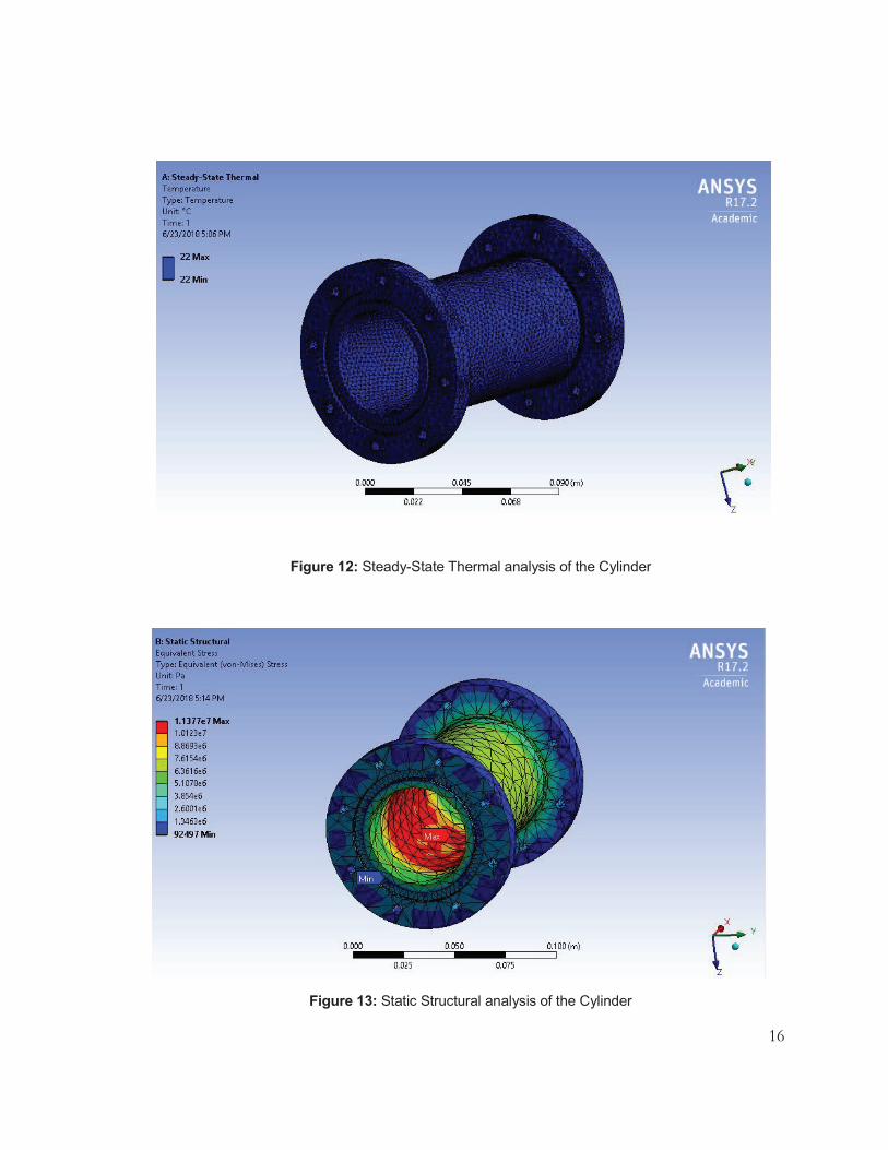
Since, the temperature was constant, the temperature distribution yielded from thermal analysis

was uniform, as shown in figure 12 for the cylinder. This thermally analyzed model was then

imported for structural analysis, yielding in structural distribution as shown in figure 13, for the

cylinder. For all the FEA analyses, coarse mesh was used for stainless steel material at 22 ْC

temperature.

(1)

15

Figure 10: Thermal boundary condition for the Cylinder

Figure 11: Structural boundary conditions for the Cylinder

16

Figure 12: Steady-State Thermal analysis of the Cylinder

Figure 13: Static Structural analysis of the Cylinder

17

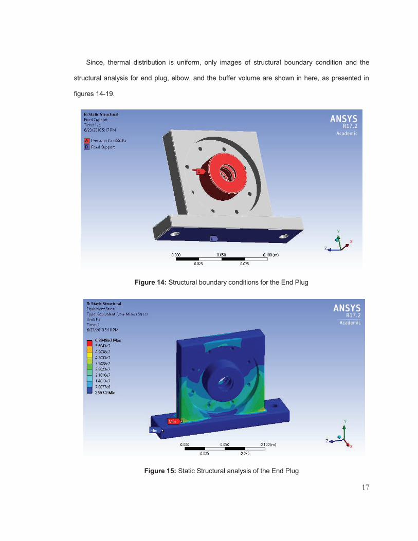
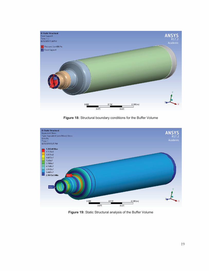
Since, thermal distribution is uniform, only images of structural boundary condition and the

structural analysis for end plug, elbow, and the buffer volume are shown in here, as presented in

figures 14-19.

Figure 14: Structural boundary conditions for the End Plug

Figure 15: Static Structural analysis of the End Plug

18

Figure 16: Structural boundary conditions for the Elbow

Figure 17: Static Structural analysis of the Elbow

19

Figure 18: Structural boundary conditions for the Buffer Volume

Figure 19: Static Structural analysis of the Buffer Volume

20

Table 2: Maximum stress, yield stress, and the safety factors for the designed components

Maximum Stress (Pa)

Yield Stress (Pa), at room temperature (22 ْC) [25]

Factor of Safety

Margin of Safety

Cylinder 1.14E+07 2.05E+08 18.00 17.00 End Plug 6.30E+07 2.05E+08 3.30 2.30

Elbow 7.43E+07 2.05E+08 2.80 1.80 Buffer

Volume 1.30E+08 2.05E+08 1.60 0.60

The table 2 above represents the maximum stresses that are acting on the components. Based

on the calculated factor of safety and margin of safety, from equations 2 and 3 [26], it was found

that all the designed models had positive safety margin (Margin of Safety > 0.5) and thus were safe

to be manufactured for conducting the experiments.

After completion of these analyses, the models were given to Wilson Works Inc. for

manufacturing.

The major components of the FLTR are:

Linear Actuator

A linear actuator ETH050 from Parker is used to generate the oscillating flow in the system. An

Intelligent Parker Amplifier (IPA) is used as the drive that is controlled by ACR-View software [27].

Figure 20 shows Parker’s linear actuator, with IPA, and sensors mounted on the linear actuator

along with the circuits. ACR-View communicates with the IPA via an Ethernet cable; also, the

sensors communicate with IPA via VM25 cable which can be seen going from the circuit to the IPA

drive.

(2)

(3)

21

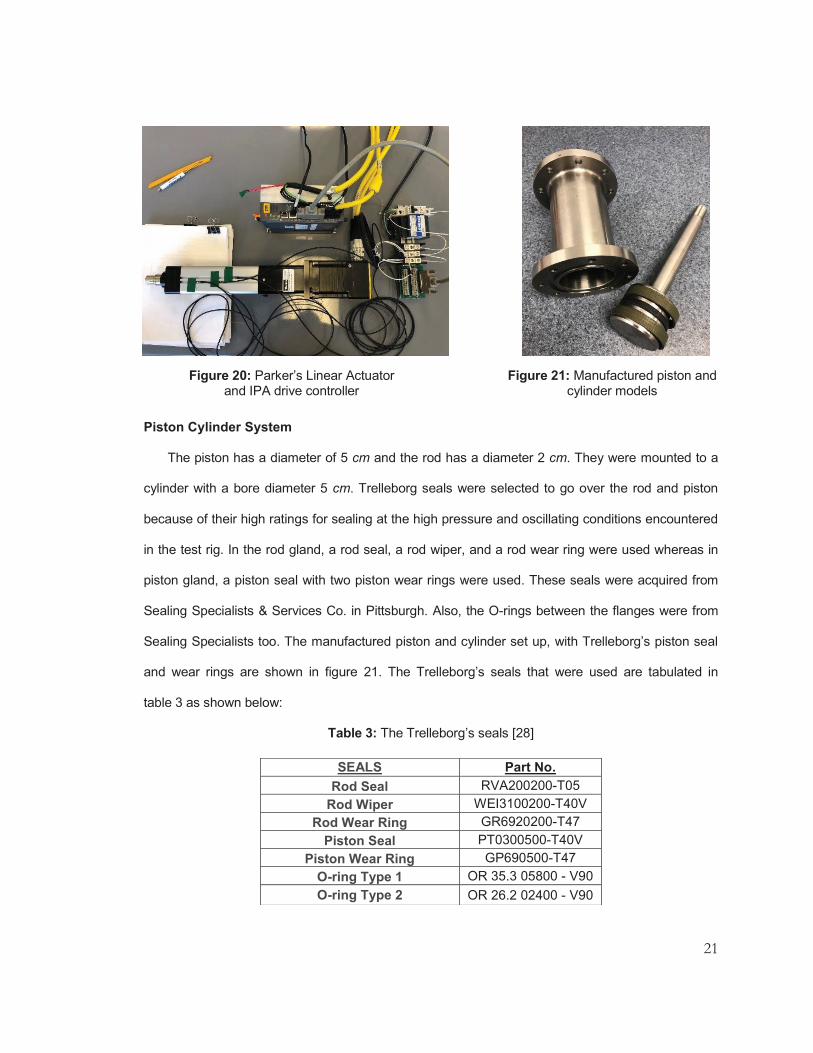
Piston Cylinder System

The piston has a diameter of 5 cm and the rod has a diameter 2 cm. They were mounted to a

cylinder with a bore diameter 5 cm. Trelleborg seals were selected to go over the rod and piston

because of their high ratings for sealing at the high pressure and oscillating conditions encountered

in the test rig. In the rod gland, a rod seal, a rod wiper, and a rod wear ring were used whereas in

piston gland, a piston seal with two piston wear rings were used. These seals were acquired from

Sealing Specialists & Services Co. in Pittsburgh. Also, the O-rings between the flanges were from

Sealing Specialists too. The manufactured piston and cylinder set up, with Trelleborg’s piston seal

and wear rings are shown in figure 21. The Trelleborg’s seals that were used are tabulated in

table 3 as shown below:

Table 3: The Trelleborg’s seals [28]

SEALS Part No. Rod Seal RVA200200-T05

Rod Wiper WEI3100200-T40V Rod Wear Ring GR6920200-T47

Piston Seal PT0300500-T40V Piston Wear Ring GP690500-T47

O-ring Type 1 OR 35.3 05800 - V90 O-ring Type 2 OR 26.2 02400 - V90

Figure 20: Parker’s Linear Actuator and IPA drive controller

Figure 21: Manufactured piston and cylinder models

22

Regenerator and Heat Rejecter

This study mainly focused on the heater head assembly which includes a heater head vessel

with hot heat exchanger tubes, an additively manufactured foil-type regenerator- the internal heat

storage unit, and a heat rejecter- the cold heat exchanger. The additively manufactured regenerator

of Inconel 718 is shown in figure 22(a), whereas a heat rejecter made of aluminum is presented in

figure 22(b).

(a) (b)

Figure 22: (a) Additively manufactured Regenerator (b) Heat rejecter

Buffer Volume

The buffer volume is the large cylindrical vessel shown in figure 8. It ensures that the pressure

differences even out in its huge volume and that there is no compression effects; which means the

prevailing pressure drop will be mostly due to frictional pressure drop in the test section. This also

results in a nearly sinusoidal and spatially uniform flow distribution in the test section [29].

Vibration Isolators

Neoprene rubber mounts and sheets are used to isolate the vibration generated from the

oscillating motion of the piston.

Balance System

To address the alignment issue between the linear actuator and the piston in the cylinder, a

balance system has been constructed. The balance system basically consists of a large flat

aluminum plate on which a number of supports are used to position the actuator and cylinder to the

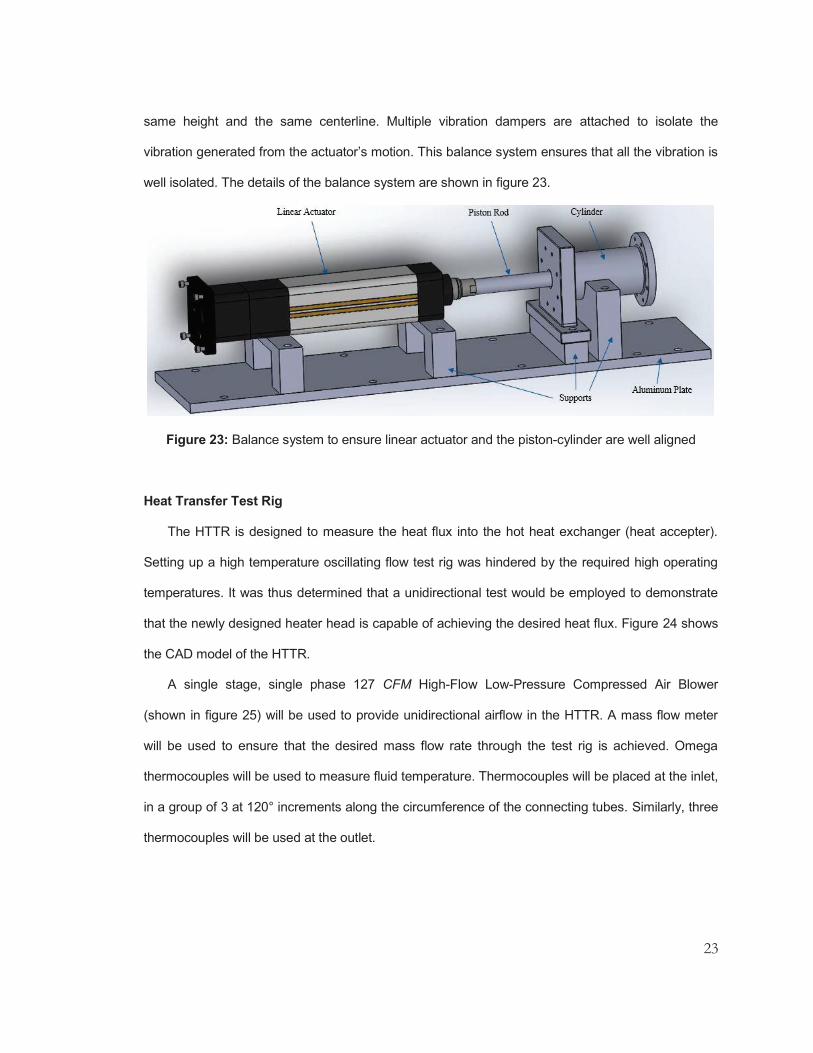
23

same height and the same centerline. Multiple vibration dampers are attached to isolate the

vibration generated from the actuator’s motion. This balance system ensures that all the vibration is

well isolated. The details of the balance system are shown in figure 23.

Figure 23: Balance system to ensure linear actuator and the piston-cylinder are well aligned

Heat Transfer Test Rig

The HTTR is designed to measure the heat flux into the hot heat exchanger (heat accepter).

Setting up a high temperature oscillating flow test rig was hindered by the required high operating

temperatures. It was thus determined that a unidirectional test would be employed to demonstrate

that the newly designed heater head is capable of achieving the desired heat flux. Figure 24 shows

the CAD model of the HTTR.

A single stage, single phase 127 CFM High-Flow Low-Pressure Compressed Air Blower

(shown in figure 25) will be used to provide unidirectional airflow in the HTTR. A mass flow meter

will be used to ensure that the desired mass flow rate through the test rig is achieved. Omega

thermocouples will be used to measure fluid temperature. Thermocouples will be placed at the inlet,

in a group of 3 at 120° increments along the circumference of the connecting tubes. Similarly, three

thermocouples will be used at the outlet.

24

In order to simulate and test the heat flux of the Inconel heater head, a heating system is being

designed; schematic and the system design are shown respectively in figures 26 and 27. It mainly

consists of coil heaters and a recuperator. In this heating system, after the cold gas passes through

the heater, a hot gas with a temperature of about 1400 °C will be generated. Then the hot gas will

diffuse and pass across the tubes of the heater head to heat up the working gas (air/Helium) in the

tubes, to the desired working temperature (810 °C).

The main purpose of the recuperator is to recover heat from exhaust gas. This hot exhaust gas

passes through shell-tube heat exchanger wherein atmospheric air is blown in the tubes to cool

down this hot air, which on the other hand heats up the incoming air. The heated air then moves

into the heating section to further receive heat, thereby increasing the efficiency of this heating

system. This whole process also ensures that the exhaust air from this heater gets to relatively low

temperature when released to the atmosphere for the safety of the personnel and equipment

around the test rig.

Figure 24: CAD model of the Heat Transfer Test Rig

Figure 25: Air Blower for the Heat Transfer Test Rig

25

Figure 26: Schematic of the Heater Design

Figure 27: Layout of the Heater Design

26

The heating system consists of three parts, Coils- for heating the air, Chamber- to mix the hot

gas, and Air flow diffuser- to ensure that the hot air flows across the heater head tubes uniformly.

In the heating system, as shown in figures 26 and 27, the coils are the main components.

These heating coils are rated for higher temperature, up to 1850 ْC, and after further analyses if

these coils work, then they will be acquired from Micropyretics Heaters International (MHI).

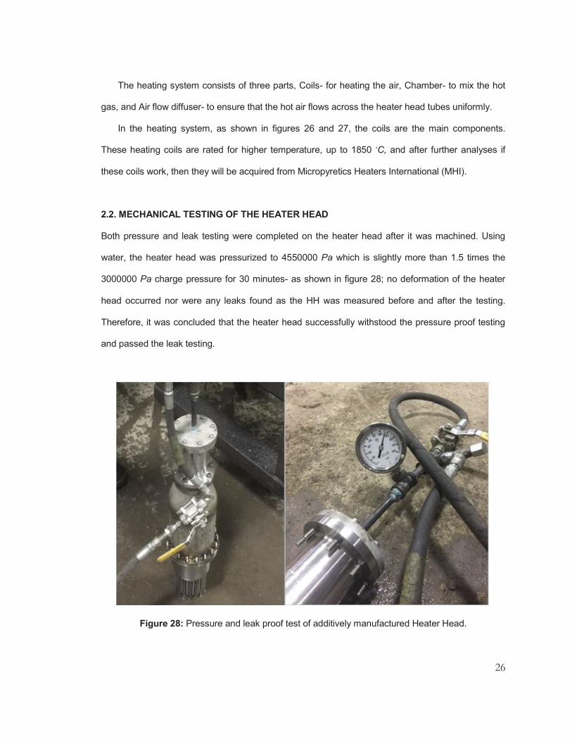
2.2. MECHANICAL TESTING OF THE HEATER HEAD

Both pressure and leak testing were completed on the heater head after it was machined. Using

water, the heater head was pressurized to 4550000 Pa which is slightly more than 1.5 times the

3000000 Pa charge pressure for 30 minutes- as shown in figure 28; no deformation of the heater

head occurred nor were any leaks found as the HH was measured before and after the testing.

Therefore, it was concluded that the heater head successfully withstood the pressure proof testing

and passed the leak testing.

Figure 28: Pressure and leak proof test of additively manufactured Heater Head.

27

2.3. PROCEDURE

FLTR Testing

After an iterative design process, the design shown above in figure 8 was finalized. Based on the

Sage simulation results and using the similarity principle for the maximum Reynolds number (Remax)

of 7694 and Valensi number (Va) of 19.3, the pressure and frequency of the system can be

determined.

For one case, the system was first charged to the desired pressure of 500000 Pa absolute with

air at room temperature of 20 ْC, where the corresponding density and dynamic viscosity of air are

5.96 kg/m3 and 1.83e-5 Pa.s, respectively. Using equations 4-17, mass flow rate and air velocity

can be estimated by matching Sage predicted Reynolds Number of Remax = 7694 at 6 Hz and

Valensi number of Va = 19.2. The calculated air velocity is 9.43 m/s, which is corresponding to a

mass flow rate of 4.14e-3 kg/s and piston velocity of 0.35 m/s. At this velocity, the amplitude of the

piston motion is 9.38 mm, and the stroke length is 18.76 mm.

28

In equation 4, mean Reynolds number (Remean) comes from Sage simulation results. Based on

the given temperature and pressure of the working fluid, corresponding density (ρgas) and dynamic

viscosity (μgas) can be found, and then using equation 4, the mean velocity of the gas (vmean-gas) can

be found.

Similarly, equation 5 represents the Valensi Number (Va). Va depends on angular frequency

(ω), kinematic viscosity (νgas) of gas, and the area of heat accepter tubes (Atube).

Equation 9 shows that the mass flow rate of the gas (mgas) is the product of gas density, gas

mean velocity, and the area of all heat accepter tubes.

Equation 10 can be used to calculate the mass flow rate across the piston, which is a product of

density of the gas, velocity of the piston (vpiston), and the cross-sectional area of the piston (Apiston).

Based on equation 11, equations 9 and 10 can be equated to find the velocity of the piston.

Equation 12 represents the distance equation which is widely used in case of sinusoidal

motions. Here, xp is the amplitude of the sinusoidal motion and the distance x is a multiple of

amplitude and the sine of angular velocity (ω) and time (t). Equation 13 is the velocity equation, or

basically a derivative of the equation 12. For this study, only ‘maximum magnitude’ is considered,

so equation 13 can be refined to get equation 14, which is used to calculate the amplitude from the

piston velocity derived from equation 11. The stroke length is the double of the amplitude as shown

in equation 17.

The linear actuator can be programmed and controlled using ACR-View for the oscillating

motion. As the piston moves forward, the air is forced to flow from the cylinder to the heat rejecter,

then through the fine regenerator openings to the heat accepter tubes of the heater head, and

continue on to the inner part of heater head from which the air exits to the buffer volume. When the

piston moves backward, the air is retracted back, and the flow occurs in the exact opposite

direction, leaving the buffer volume first and reaching into the cylinder, eventually. This process

happens repeatedly at the set frequency. This oscillating flow is illustrated in figure 29.

29

Figure 29: Illustration of the oscillating flow in FLTR

HTTR Testing

The air blower is used to provide unidirectional airflow in the heat flux testing experiment. As

this is a unidirectional open flow test rig, the heated fluid is released into the atmosphere, as shown

in figure 30.

Figure 30: Illustration of the unidirectional flow in HTTR

30

C H A P T E R 3 . D A T A A C Q U I S I T I O N A N D P R O C E S S I N G

Since most of the work done so far was primarily on FLTR, the discussion of data acquisition and

post-processing will focus on FLTR data only.

Data acquisition for this study consisted mainly of 3 parts- collecting data from pressure

transducers, collecting piston’s position, and synchronizing them together for data processing. The

data acquisition must be performed taking into account the fact that to get sufficiently converged

ensemble-averages, data from 50 to 100 cycles are required. To get sufficient temporal resolution

and by considering sinusoidal motion, data needs to be taken at least every 0.5 ْ i.e. at least 720

data points in each cycle [18, 30].

3.1. COLLECTING DATA FROM PRESSURE TRANSDUCERS

Two pressure transducers (Kistler’s 601 C) are placed at the inlet (below the heat rejecter) and

outlet (before the buffer volume) to measure the pressure drop of the flow for the flow loss

measurement. Similarly, a high-accuracy and corrosion-resistant pressure gauge with a range of 0-

160 psi was used to get the static charge pressure of the system. The picked up analog signal from

the Kistler’s dynamic sensors was converted to digital form and recorded via LabVIEW code using

the National Instruments’ DAQ system. Figure 31 shows the DAQ system that is being used for this

experiment. Specifically, NI 9234 module will be used on cDAQ-9178 chassis for the pressure

measurement.

3.2. COLLECTING PISTON’S POSITION DATA

There is an encoder inbuilt with the Parker’s BE342HJ-KPSN motor which is being used in the

linear actuator. This is a 2000-line incremental encoder with quadrature feature (differential signals),

which runs at 8000 pulses per revolution (ppr). The feedback cable coming out of the IPA drive was

cut and the wires (4 channels: A+, A-, B+, and B-) that carry encoder signal was connected to an

31

NI 9411 module. The NI 9411 is a counter input module that reads the data from those four

channels of the feedback cable and gives out linear position.

3.3. SYNCHRONIZATION OF POSITION AND PRESSURE DATA

Once piston’s position data and pressure data are available, synchronization of these data is

required.

A set of experiments were run to see how many data points are outputted every cycle. The

beginning of the first cycle is based on first zero-crossing. The information tabulated in table 4 is

average number of points that the linear actuator outputs every cycle at the shown frequency,

piston’s amplitude, and the system’s charged pressure conditions; the number varies in a vast

range.

Figure 31: National Instruments’ cDAQ 9178 and modules NI 9234, NI 9213, and NI 9411 (from left to right)

32

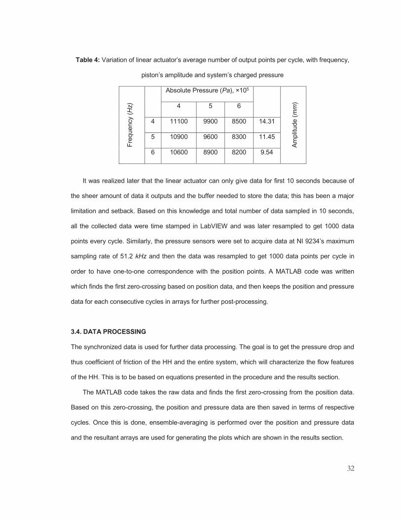
Table 4: Variation of linear actuator’s average number of output points per cycle, with frequency,

piston’s amplitude and system’s charged pressure

It was realized later that the linear actuator can only give data for first 10 seconds because of

the sheer amount of data it outputs and the buffer needed to store the data; this has been a major

limitation and setback. Based on this knowledge and total number of data sampled in 10 seconds,

all the collected data were time stamped in LabVIEW and was later resampled to get 1000 data

points every cycle. Similarly, the pressure sensors were set to acquire data at NI 9234’s maximum

sampling rate of 51.2 kHz and then the data was resampled to get 1000 data points per cycle in

order to have one-to-one correspondence with the position points. A MATLAB code was written

which finds the first zero-crossing based on position data, and then keeps the position and pressure

data for each consecutive cycles in arrays for further post-processing.

3.4. DATA PROCESSING

The synchronized data is used for further data processing. The goal is to get the pressure drop and

thus coefficient of friction of the HH and the entire system, which will characterize the flow features

of the HH. This is to be based on equations presented in the procedure and the results section.

The MATLAB code takes the raw data and finds the first zero-crossing from the position data.

Based on this zero-crossing, the position and pressure data are then saved in terms of respective

cycles. Once this is done, ensemble-averaging is performed over the position and pressure data

and the resultant arrays are used for generating the plots which are shown in the results section.

Freq

uenc

y (H

z)

Absolute Pressure (Pa), ×105

Ampl

itude

(mm

) 4 5 6

4 11100 9900 8500 14.31

5 10900 9600 8300 11.45

6 10600 8900 8200 9.54

33

For the uncertainty analysis, MATLAB code is modified with addition of extra loops which take

care of additional number of experiments, and then allocates the array accordingly. Eventually,

standard deviations are taken over the averaged values and then maximum and minimum pressure

drops are found in order to report their uncertainties from the experimentation.

The code is also adjusted to read in Sage and CFD predicted Reynolds number, pressure drop,

and coefficient of friction values. Once read in, they are then plotted with their corresponding

experimental values for comparisons, as presented in the results section.

The used MATLAB code is presented in the Appendix.

34

C H A P T E R 5 . R E S U L T A N D D I S C U S S I O N

The Sage predicted results are for the case at 60 Hz, 4000000 Pa, 67 ْC rejection temperature, and

810 ْC hot end temperature. The mean Reynolds and Valensi numbers for each component are

also listed in the Sage results. These two parameters must be matched in the experiments to

ensure that results are comparable to the Sage data. Table 5 lists the expected values of mean

pressure, friction factor correlation, mass flow rate, friction factor, and mean Reynolds number for

the regenerator at a mean Valensi number of 3.105. These values are based on the first term

approximation of the Fourier series. For the regenerator, the hydraulic diameter is 6.0e-4 m and the

roughness is 6e-9 m. In addition, the results of the regenerator flow loss will be compared to those

of a woven screen and random fiber regenerator previously reported by Gedeon and Wood. Those

correlations are as follows in equations 18 and 19 [11]:

Here, Cf is the coefficient of friction.

Table 5: Expected results for regenerator as predicted by Sage

The FLTR is used to measure the pressure drop across the entire heater head system (heat

acceptor, regenerator, and heat rejecter). But it can also be used to determine the pressure drop in

the heat acceptor alone or heat acceptor with regenerator, or heat acceptor with heat rejecter.

At first, an experiment can be conducted with the heat acceptor alone. The measured pressure

drop and thus friction factor can be compared to the correlations for both laminar and turbulent flow

within a circular tube. If a significantly higher than expected friction factor occurs, it is an indication

Mean Pressure (Pa), ×105 Friction Factor, Cf [11] Mass flow

rate (kg/s) Re

Regenerator 39.5

0.02 184.0

(18)

(19)

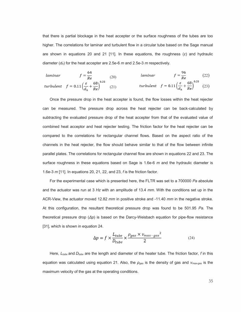
35

that there is partial blockage in the heat accepter or the surface roughness of the tubes are too

higher. The correlations for laminar and turbulent flow in a circular tube based on the Sage manual

are shown in equations 20 and 21 [11]. In these equations, the roughness (ε) and hydraulic

diameter (dh) for the heat accepter are 2.5e-6 m and 2.5e-3 m respectively.

Once the pressure drop in the heat accepter is found, the flow losses within the heat rejecter

can be measured. The pressure drop across the heat rejecter can be back-calculated by

subtracting the evaluated pressure drop of the heat accepter from that of the evaluated value of

combined heat acceptor and heat rejecter testing. The friction factor for the heat rejecter can be

compared to the correlations for rectangular channel flows. Based on the aspect ratio of the

channels in the heat rejecter, the flow should behave similar to that of the flow between infinite

parallel plates. The correlations for rectangular channel flow are shown in equations 22 and 23. The

surface roughness in these equations based on Sage is 1.6e-6 m and the hydraulic diameter is

1.6e-3 m [11]. In equations 20, 21, 22, and 23, f is the friction factor.

For the experimental case which is presented here, the FLTR was set to a 700000 Pa absolute

and the actuator was run at 3 Hz with an amplitude of 13.4 mm. With the conditions set up in the

ACR-View, the actuator moved 12.82 mm in positive stroke and -11.40 mm in the negative stroke.

At this configuration, the resultant theoretical pressure drop was found to be 501.95 Pa. The

theoretical pressure drop (Δp) is based on the Darcy-Weisbach equation for pipe-flow resistance

[31], which is shown in equation 24.

Here, Ltube and Dtube are the length and diameter of the heater tube. The friction factor, f in this

equation was calculated using equation 21. Also, the ρgas is the density of gas and vmax-gas is the

maximum velocity of the gas at the operating conditions.

(24)

(20)

(21)

(22) (23)

36

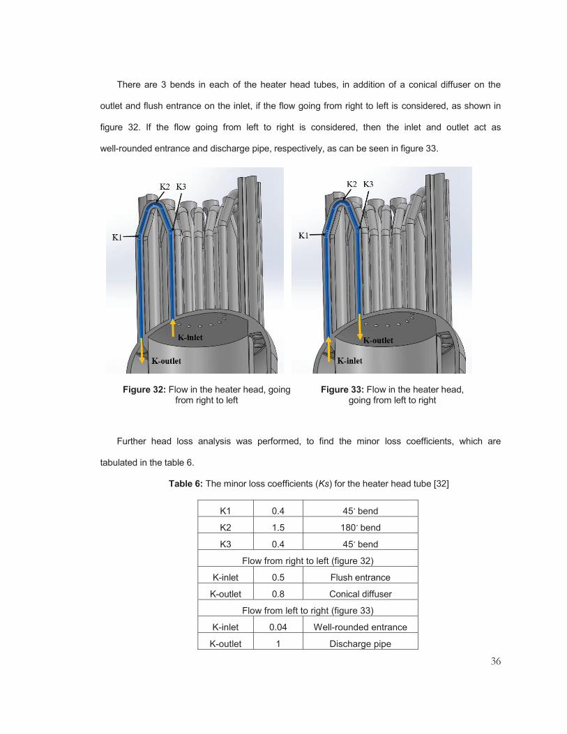
There are 3 bends in each of the heater head tubes, in addition of a conical diffuser on the

outlet and flush entrance on the inlet, if the flow going from right to left is considered, as shown in

figure 32. If the flow going from left to right is considered, then the inlet and outlet act as

well-rounded entrance and discharge pipe, respectively, as can be seen in figure 33.

Further head loss analysis was performed, to find the minor loss coefficients, which are

tabulated in the table 6.

Table 6: The minor loss coefficients (Ks) for the heater head tube [32]

K1 0.4 bend ْ45

K2 1.5 bend ْ180

K3 0.4 bend ْ45

Flow from right to left (figure 32)

K-inlet 0.5 Flush entrance

K-outlet 0.8 Conical diffuser

Flow from left to right (figure 33)

K-inlet 0.04 Well-rounded entrance

K-outlet 1 Discharge pipe

Figure 32: Flow in the heater head, going from right to left

Figure 33: Flow in the heater head, going from left to right

37

These minor loss coefficients (Ks) were used in equation 25 to get combined head loss (hL),

from which final pressure drop (Δpfinal) was calculated using equation 26 [33]. Here, g is the

acceleration due to gravity (9.8 m/s2).

The final pressure drop for this case was found to be 1183.96 Pa when going from right to left

as in figure 32 and 1134.7 Pa when going from left to right as can be seen in figure 33.

5.1 PRELIMINARY EXPERIMENTAL RESULTS

Following are the results after the experimental values were collected via LabVIEW and processed

in MATLAB. At 3 Hz, after allocating the data in arrays based on first zero-crossing of the position, a

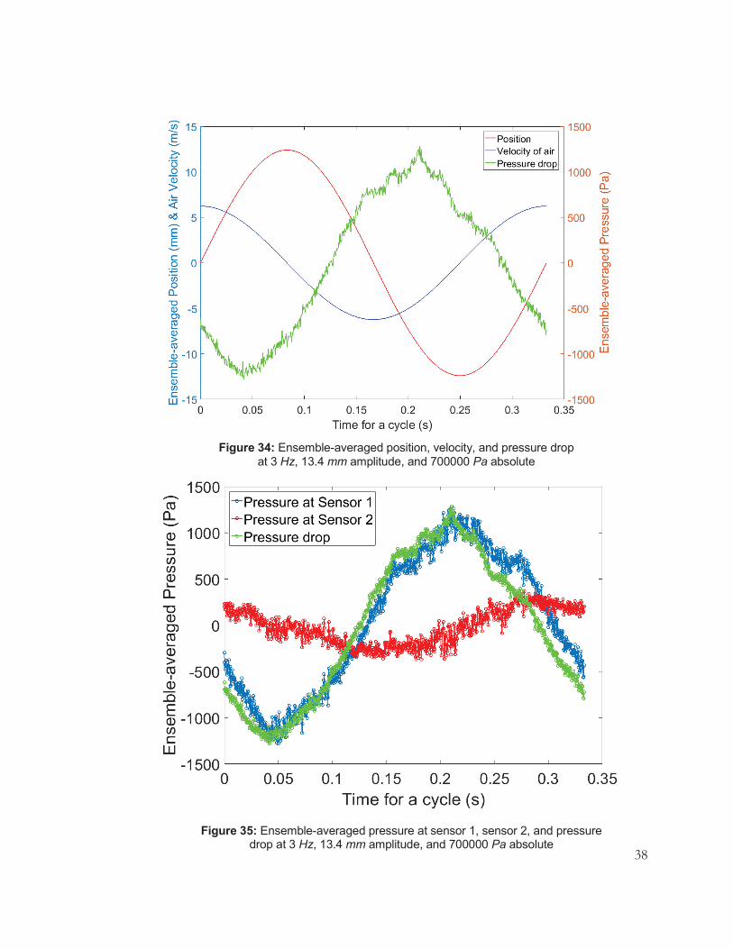
total of 29 cycles were used to get these plots, from 10 seconds worth of data. Figure 34 shows the

ensemble-averaged position, velocity, and pressure drop against the total time for a cycle. It can be

seen that the peak position magnitudes were 12.40 mm and -12.09 mm, the air velocity’s peak

magnitudes were 6.24 m/s and 0.01 m/s, whereas the pressure drop peaked at 1281.7 Pa and

-1281.7 Pa. Here, pressure drop was the difference of pressure values from sensor 1 and sensor 2.

These experimental pressure drops were higher than the theoretical; the possible causes for

this could be higher surface roughness and partial restriction of flow in the heater head tubes.

Similarly, figure 35 shows the ensemble-averaged pressure from sensor 1, sensor 2, and the

corresponding pressure drop across total time for a cycle.

(25)

(26)

38

Figure 34: Ensemble-averaged position, velocity, and pressure drop at 3 Hz, 13.4 mm amplitude, and 700000 Pa absolute

Figure 35: Ensemble-averaged pressure at sensor 1, sensor 2, and pressure drop at 3 Hz, 13.4 mm amplitude, and 700000 Pa absolute

39

The ensemble-averaged raw pressure data from each sensor was curve fitted in MATLAB to

ensure if the collected data was sinusoidal, and the following perfect sine curves were realized, as

shown in figures 36 and 37.

Figure 36: Ensemble-averaged pressure at sensor 1 at 13.4 mm amplitude, and 700000 Pa absolute, curve fitted to Sine wave in MATLAB

Figure 37: Ensemble-averaged pressure at sensor 2 at 13.4 mm amplitude, and 700000 Pa absolute, curve fitted to Sine wave in MATLAB

40* CFD data from Dr. Laura Solomon

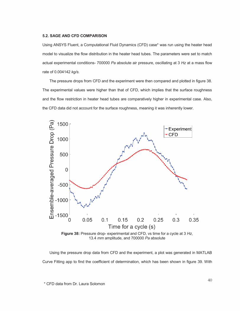
5.2. SAGE AND CFD COMPARISON

Using ANSYS Fluent, a Computational Fluid Dynamics (CFD) case* was run using the heater head

model to visualize the flow distribution in the heater head tubes. The parameters were set to match

actual experimental conditions- 700000 Pa absolute air pressure, oscillating at 3 Hz at a mass flow

rate of 0.004142 kg/s.

The pressure drops from CFD and the experiment were then compared and plotted in figure 38.

The experimental values were higher than that of CFD, which implies that the surface roughness

and the flow restriction in heater head tubes are comparatively higher in experimental case. Also,

the CFD data did not account for the surface roughness, meaning it was inherently lower.

Using the pressure drop data from CFD and the experiment, a plot was generated in MATLAB

Curve Fitting app to find the coefficient of determination, which has been shown in figure 39. With

Figure 38: Pressure drop- experimental and CFD, vs time for a cycle at 3 Hz, 13.4 mm amplitude, and 700000 Pa absolute

41

R2 of 0.9686, this plot clarifies that even though the magnitude of the CFD and experimental

pressure drop are not equal, they follow the same trend line and fit together very well.

Figure 40 below shows the plot of coefficient of friction (Cf) against the Reynolds number (Re)

for experimental and theoretical cases. For experimental case, data was collected from 6 different

experiments by varying the amplitudes and thus, the velocities at the same frequency of 3 Hz, to get

6 different maximum Reynolds number and corresponding 6 different maximum Cf. The Cf-max

calculations were based on equation 27, which is simple modification of equation 24.

For the theoretical case, the correlation from Sage for turbulent tube flow, as presented in

equation 27 was used to find the friction factor. This friction factor was then used along with the

minor head losses that account for the bends in the HH tubes, as shown in table 6, to find the

combined head loss using equation 25. Using equation 26, the total pressure drop was then found.

Eventually, using equation 27, theoretical Cf was found.

(27)

Figure 39: Ensemble-averaged pressure drop from CFD vs. the ensemble-averaged pressure drop from experiment, for Coefficient of Determination, R2 being 0.9686.

42

From the plot 40, it can be seen that the experimental Cf is clearly larger than that of the

theoretical Cf, at the same Reynolds number, which again ensured that there was flow restriction in

the tubes and the surface roughness was higher than what had been considered in Sage.

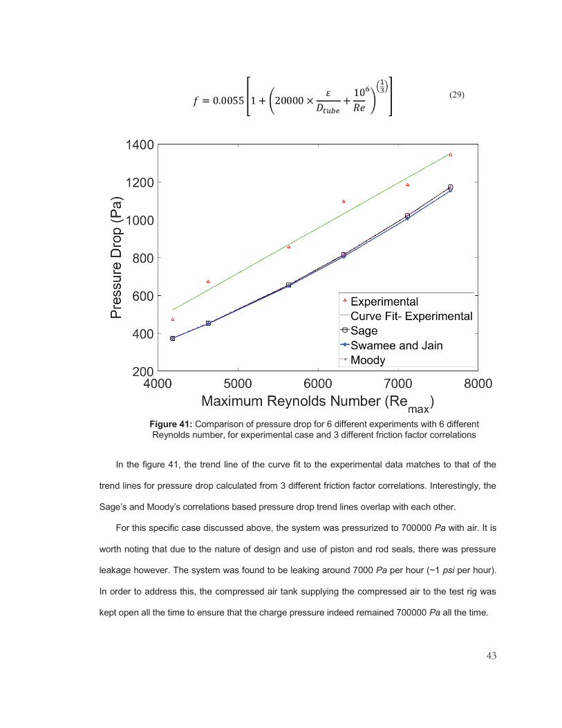
From the figure 41, it can be seen that the resulting pressure drop for experimental case is

higher compared to the pressure drop using three different correlations for the friction factor- for

same surface roughness of 2.5 μm. This yields that the heater head has tubes, which have higher

surface roughness as to what Sage is using, which is 2.5 μm. The three correlations used were for

friction factor at turbulent flow conditions- from Sage based on equation 21, Swamee and Jain’s

correlation based on equation 28 [33], and Moody’s correlation based on equation 29 [34].

Figure 40: Maximum coefficient of friction (Cf-max) versus maximum Reynolds number (Remax) – comparing Experimental and Theoretical Cf-max at same Remax

(28)

43

In the figure 41, the trend line of the curve fit to the experimental data matches to that of the

trend lines for pressure drop calculated from 3 different friction factor correlations. Interestingly, the

Sage’s and Moody’s correlations based pressure drop trend lines overlap with each other.

For this specific case discussed above, the system was pressurized to 700000 Pa with air. It is

worth noting that due to the nature of design and use of piston and rod seals, there was pressure

leakage however. The system was found to be leaking around 7000 Pa per hour (~1 psi per hour).

In order to address this, the compressed air tank supplying the compressed air to the test rig was

kept open all the time to ensure that the charge pressure indeed remained 700000 Pa all the time.

(29)

Figure 41: Comparison of pressure drop for 6 different experiments with 6 different Reynolds number, for experimental case and 3 different friction factor correlations

44

After completion of FLTR analysis and manufacturing of Heater system, experiments on the

HTTR would be run at variable conditions to get the values closer to what Sage predicts, as

presented in table 7; it would complete the heat transfer characterization of the HH.

Table 7: Expected experimental results from HTTR based on Sage [35]

Diameter 0.0025 m

Length of each tubes 0.1912 m

Surface Area of Heater Head, for all 15 tubes 0.0225 m2

Total Heat In 2820 W

Total Heat Flow over Heater Head 118 kW/m2

5.3 UNCERTAINTY ANALYSIS

No measurement is free of inaccuracies, and the appropriate concept to expressing such

inaccuracies is an “uncertainty”, which is provided by “uncertainty analysis”. Generally, the value

reported from measurement is its central tendency, usually the mean, and the uncertainty then is

the dispersion of the measurement, expressed in terms of standard deviation. This uncertainty is

calculated from repeated experimental trials [36].

For this study, an uncertainty analysis was performed over the data collected at 700000 Pa

absolute pressure of air at 20 ْC. The existing MATLAB code was modified to perform uncertainty

analysis. For the collected pressure drop, the uncertainty of the data processing was addressed in

this MATLAB code by taking the average of the averages of pressure drops in each cycles of an

experiment over N-number of experiments. As data from only (N=) 11 experiments, all at same

operating conditions, was considered for uncertainty analysis, Student’s t-distribution was used

(N>30, normal distribution can be considered). The results from this analysis are presented in the

following table 8.

45

Table 8: The uncertainty in the maximum and minimum pressure drop

Max. Pressure Drop Min. Pressure Drop

Mean 1083.2 Pa -1113.3 Pa

Standard Deviation 116.9 Pa 77.8 Pa

No. of experiment, N 11

v (N-1) 10

t (at 95 % confidence) [37] 1.81

Confidence limit 1083.2 ± 5.9 % Pa -1113.3 ± 3.8% Pa

This confidence limit corresponds to an average uncertainty of about 5.9 % for maximum

pressure drop and to an average uncertainty of about 3.8 % for minimum pressure drop in the

system.

After taking the average of the ensemble-averaged position and pressure, following plots were

generated as shown in figure 42 and 43. From figure 42, it can be seen that the maximum and

minimum position over a cycle were 12.40 mm and -12.06 mm, respectively. Similarly, the

maximum and minimum velocities were 6.24 m/s and 0.01 m/s, respectively.

From figure 43, it is clearly evident that the pressure drop when averaged over 11 experiments,

is turning out to be free of fluctuations and becoming more sinusoidal. The maximum and minimum

pressure drop values when averaged over 11 experiments were also relatively lower than that of an

individual experiment’s ensemble-averaged maximum and minimum pressure drops.

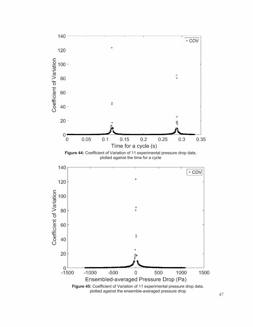
Figure 44 represents the coefficient of variation (COV) of the ensemble-averaged pressure drop

from the 11 experiments mentioned above, plotted against the time for a cycle. The COV values

tend to increase significantly as the pressure drop approaches 0- this is more apparent in figure 45,

where COV is plotted against the ensemble-averaged pressure drop. However, if only maximum

and minimum pressure drop are considered for the cycle, the COV values are good, values being

0.1079 for maximum pressure drop and 0.0699 for the minimum pressure drop.

46

Figure 42: Ensemble-averaged position, velocity, and pressure drop at 3 Hz, 13.4 mm amplitude, and 700000 Pa absolute, over 11 experiments at same operating conditions

Figure 43: Ensemble-averaged pressure drop for an experiment and for over 11 experiments at same operating conditions, at 3 Hz, 13.4 mm amplitude, and 700000 Pa absolute

47

Figure 44: Coefficient of Variation of 11 experimental pressure drop data, plotted against the time for a cycle

Figure 45: Coefficient of Variation of 11 experimental pressure drop data, plotted against the ensemble-averaged pressure drop

48

C H A P T E R 6 . C O N C L U S I O N S

After in-depth literature review on Stirling engine experimental setups, the setups in this study were

decided. To study flow loss, Flow Loss Test Rig- FLTR incorporated oscillating flow. Due to high

temperature conditions, heat flux testing could not be done using oscillating flow, and such Heat

Transfer Test Rig- HTTR design incorporated unidirectional flow.

SOLIDWORKS 2016 was used to design all components of both FLTR and HTTR. Finite

Element Analysis using ANSYS Mechanical 2017 was performed over the designed models to

ensure they withstand the operating conditions- 2000000 Pa working pressure at room temperature.

The finalized models were then given to Wilson Works for manufacturing.

Parker made linear actuator was used as the oscillating flow generator for FLTR, whereas as

Low-Pressure Compressed Air Blower was decided to be used as the unidirectional flow generator

for HTTR. In order to meet requirements of the heat flux testing, a novel ‘heater and recuperator’

system is in design process currently.

For FLTR, Trelleborg’s high efficient rod and piston seals were used. Kistler 601 C pressure

transducers were used in order to measure the dynamic pressure of the system. The signals from

these sensors were read via NI 9234 on cDAQ 9178. Additionally, NI 9411 was used to read linear

actuator’s position. In order to read signals from these NI modules, codes were written in LabVIEW

2011. For the post processing of data collected from LabVIEW, codes were written in MATLAB

2016.

With the completion of FLTR design and fabrication, the experimental setup was readied by

putting all essential components together. Experiments were then conducted at various flow

conditions to investigate the flow losses in the heater head. From the preliminary results, it was

found that the resulting pressure drop across the heater head tubes was higher than theoretical and

CFD predictions, based on figure 38. From figures 40 and 41, it was found that the experimentally

calculated Cf was higher than that of Sage. It can thus be concluded that due to presence of higher

surface roughness and flow restrictions in the tubes due to partial blockages of the flow path, the

49

resulting pressure drop and the coefficient of friction are higher in experimental conditions

compared to that of Sage and CFD predictions.

Furthermore, uncertainty analysis was performed on the collected pressure drop. Using the

student’s t-distribution, with 95% confidence, an average uncertainty of about 5.9 % and 3.8 % for

maximum and minimum pressure drop, respectively, was found.

It was also concluded that the development of the heat transfer test rig- HTTR is on right track.

The HTTR development would soon be complete, and the experiments would be run to find out

total heat flux across the heat accepter, which will determine the thermal characteristics of this

heater head.

6.1. FUTURE WORKS

In order to fully investigate the flow loss in the heater head, more effective vibration isolation

measures should be taken to isolate vibrations from the system. It would be beneficial if the

pressure transducer 2 would be shifted to top side of the elbow, so that it does not face directly to

linear actuator motion. Multiple experiments at variable conditions should be run on the FLTR to

investigate in detail the effects of presence of elbow before the heater head, the effects of change in

amplitude, and the effects of change in frequency on the pressure drops, in order to fully

characterize the flow losses in the heater head.

For the heat flux testing, the designed heater and recuperator system to be used should be

robust and should be able to get the flow within the heater head tubes to the desired temperature of

~750 ْC- this will ensure more realistic heat flux characterization of the heater head.

50

C H A P T E R 7 . R E F E R E N C E S

[1] “Stirling engine”, Wikipedia, URL: https://en.wikipedia.org/wiki/Stirling_engine [retrieved 10 June

2018]

[2] “Understanding Stirling engines in Ten Minutes or Less”, American Stirling Company, URL:

https://www.stirlingengine.com/download/9-12.pdf [retrieved 15 July 2017]

[3] “Background and Information”, Ohio University, URL: https://www.ohio.edu/mechanical/stirling-

/intro.html [retrieved 11 June 2018]

[4] “Lean and Data-Driven: Remembering the Founder of a World-Class Renewable Energy

Company”, Ohio University, URL: https://www.ohio.edu/mechanical/stirling/engines/William-

Beale-memorial.pdf [retrieved 15 July 2017]

[5] Werle, C.A.B., Imhoff, J., Hey, H.L., & Pinheiro, J.R. (Nov. 2017). Stirling Cycle Machines for

Combined Heat and Power. 19th International Congress of Mechanical Engineering. Brasilia,

DF, November 5-9, 2017

[6] “Beta Type Stirling Engines”, Ohio University, URL: https://www.ohio.edu/mechanical/stirling/-

engines/beta.html [retrieved 11 June 2018]

[7] “Free Piston Stirling Engines – Nice Technology for Tinkerers”, Tallbloke’s Talkshop, URL:

https://tallbloke.wordpress.com/2013/04/19/free-piston-stirling-engines-nice-technology-for-

tinkerers/ [retrieved 10 June 2018]

[8] Qiu, S., Gao, Y., Rinker, G., Solomon, L., Yanaga, K., & Yadav, P.K. (2018). Development of an

Advanced Free-Piston Stirling Engine for Micro Combined Heat and Power Application. Applied

Energy. Manuscript submitted for publication

[9] Tanaka, M., Yamashia, I., & Chisaka, F. (1990). Flow and Heat Transfer Characteristics of the

Stirling Engine Regenerator in an Oscillating Flow. JSME Int J. 33(2):283–9.

[10] Solomon, L., Qiu, S. (June 2018). Computational analysis of external heat transfer for a tubular

Stirling convertor. Applied Thermal Engineering, 134-141.

doi: 10.1016/j.applthermaleng.2018.03.070

51

[11] Qiu, S., “ARPA-E GENSETS Q2 2018,” April 2018.

[12] Gao, Y., Qiu, S., & Rinker, G. (2018). Design and Optimization of a Stirling Engine Heater

Head. Energy Conversion and Management. Manuscript submitted for publication

[13] Alfarawi, S., AL-Dadah, R., & Mahmoud, S. (Sept. 2016). Influence of phase angle and dead

volume on gamma- type Stirling engine power using CFD simulation. Energy Conversion and

Management, 130-140. doi: 101016/jenconman201607016

[14] Costa, S.C., Barreno, I., Tutar, M., Esnaola, J.A., & Barrutia, H. (Jan. 2015). The thermal non-

equilibrium porous media modelling for CFD study of woven wire matrix of a Stirling

regenerator. Energy Conversion and Management, 130-140.

doi: 101016/jenconman201410019

[15] Gheith, R., Hachem, H., Aloui, F., & Ben Nasrallah, S. (Nov 2015). Experimental and

theoretical investigation of Stirling engine heater: Parametrical optimization. Energy Conversion

and Management, 285-293. doi: 101016/jenconman201507063

[16] Song, Z., Chen, J., & Yang, L. (Aug. 2015). Heat transfer enhancement in tubular heater of

Stirling engine for waste heat recovery from flue gas using steel wool. Applied Thermal

Engineering, 499-504. doi: 101016/japplthermaleng201505028

[17] “Using the Stirling Engine for Electrical Power Generation”, OkoFEN, URL: http://www.okofen-

e.com/en/chp_technologies/ [retrieved 25 April 2018]

[18] Seume, J.R. (1988), ‘An Experimental Investigation of Transition in Oscillating Pipe Flow’,

Ph.D. Dissertation, The University of Minnesota, Twin Cities- MN, USA

[19] Koester, G., Howell, S., Wood, G., & Miller, E. (1990). “Oscillating Flow Loss Test Results in

Stirling Engine Heat Exchangers.” NASA Contractor Report 182288.

[20] Kuosa, M., Saari, K., Kankkunen, & A., Tveit, T.-M., (2012). Oscillating flow in a Stirling engine

heat exchanger. Applied Thermal Engineering, Vol 45-46, 15-23.

doi: 10.1016/j.applthermaleng.2012.03.023

52

[21] Kornhauser, A. A., & Smith, J. L. Jr., (1989). Heat transfer with oscillating pressure and

oscillating flow. Proceedings of the 24th Intersociety Energy Conversion Engineering

Conference. Washington, DC: IEEE. doi: 10.1109/IECEC.1989.74802

[22] Ju, Y, Jiang, Y., Zhou, Y. (1997). Experimental study of the oscillating flow characteristics for a

regenerator in a pulse tube cryocooler. Cryogenics. Vol 38(6), 649-656.

doi: 10.1016/S0011-2275(98)00037-X

[23] Costa, S. C., Barreno, I., Prieto, J. I., González, M. A., & Garcia, D., (2012). Stirling

Regenerator Test Bench Design for Pressure Drop and Thermal Efficiency measurements.

ISEC International Stirling Engine Conference. ISBN: 978-88-8326-019-3.

[24] “Thin Walled Pressure Vessel Stress Calculations”, AmesWeb, URL: https://www.amesweb.-

info/StressStrainTransformations/StressInThinWallPressureVessel/StressInThinWallPressureV

essel.aspx [retrieved 12 June 2017]

[25] “Stainless Steel – Grade 304”, Stainless Steel directory, URL: http://askzn.co.za/stainless-

steel/tech-grade-304.htm [retrieved 15 June 2018]

[26] “Factor of safety”, Wikipedia, URL: https://en.wikipedia.org/wiki/Factor_of_safety [retrieved 15

June 2018]

[27] “Intelligent Parker Amplifier”, Parker Hannifin Corporation, URL: http://onexia.com/parker/pdf/-

ONExia-Parker-IPA-Brochure.pdf [retrieved 14 September 2017].

[28] “Hydraulic Seals- linear”, Trelleborg Sealing Solutions, URL: https://www.tss-static.com/remo-

temedia/media/globalformastercontent/downloadsautomaticlycreatedbyscript/catalogs/hydraulic

_complete_gb_en.pdf [retrieved 20 august 2017]

[29] Ibrahim, M.B., Tew, R.C. Jr. (2012). Stirling Convertor Regenerators. Boca Raton, FL: CRC

Press.

[30] Friedman, G.T. (1991), ‘Experimental Investigation of Fluid Mechanics in Oscillating Flow: A

Detailed Study at a Single Operating Point’, Master’s Thesis, The University of Minnesota, Twin

Cities- MN, USA

53

[31] “The Darcy-Weisbach Equation”, Oklahoma State University, URL: https://bae.okstate.edu/-

faculty-sites/Darcy/DarcyWeisbach/Darcy-WeisbachEq.htm [retrieved 25 May 2018]

[32] Anderson, G., Barr, R., & Benvenga, R. (2015), Minor Losses, Colorado State University, URL:

http://www.engr.colostate.edu/~pierre/ce_old/classes/CIVE%20401/projects%202015/Minor%2

0Losses%20(1).pdf [retrieved 14 June 2018]

[33] Crowe, C.T., Elger, D.F., Williams B.C., & Roberson, J.A. (2009). Engineering Fluid Mechanics.

Jefferson City: R.R. Donnelley

[34] Genic, S., Arandjelovic, I., Kolendic, P., Jaric, M., Budimir, N., & Genic, V. (2011). A review of

explicit approximations of Colebrook’s Equation. FME Transactions 29, 67-71.

[35] Qiu, S., “Sage Output 10-17-2017,” October 2017.

[36] J. Kline, S. (1985). The Purposes of Uncertainty Analysis. Journal of Fluids Engineering-

transactions of The ASME - J FLUID ENG. 107. doi: 10.1115/1.3242449.

[37] Polikar, R. (2004). Appendix D: Percentile Values tp for Student’s t Distribution with v Degrees

of freedom, ENG 0901.102.03 Freshman Engineering Clinic II-Spring 2004, URL: http://study-

lib.net/doc/8194436/examples-and-homework-questions-on-engineering-statistics [retrieved 15

June 2018]

54

C H A P T E R 8 . A P P E N D I X

The MATLAB code explained in the data processing and result section is presented in here:

…………………………………………………………………………………………………………………..

% Pawan Kumar Yadav % Stirling Engine Lab % West Virginia University % 05/23/2018 %% %CODE: % 1. To find Zero-Crossing, based on position % 2. To allocate position and pressure for each cycle based on % zero-crossing % 3. To find Ensemble-Averaged positions and pressures % 4. To perform Uncertainty Analysis- for this all the files being % considered should be representing exactly the same operating conditions %Things to be changed: Frequency, Density, mu, Amplitude sign for sine curve, %N- number of files to do uncertainty analysis on dP, no of tubes of HH %% clear close all clc %% %%% TO BE CHANGED... frequency_curve = 3.003; %Hz rho = 8.35156; %kg/m3 mu = 1.83e-5; %Pa.s no_tubes = 15; N = 11; % for now non_zero = 0; % initializing number of non-zero crossing parameter for the non-0 crossing array no_zeros = 0; % initializing number of zero crossing for the 0-crossing array pressure_1(:,1) = xlsread('Filter1000Hz_File20_v179acc0amp13.4_7barsAbs_3.003Hz.xlsx','E25:E30054'); position_1(:,1) = xlsread('Filter1000Hz_File20_v179acc0amp13.4_7barsAbs_3.003Hz.xlsx','B25:B30054');

55

%%% Individual Pressure pressure_a(:,1) = xlsread('Filter1000Hz_File20_v179acc0amp13.4_7barsAbs_3.003Hz.xlsx','C25:c30054'); pressure_b(:,1) = xlsread('Filter1000Hz_File20_v179acc0amp13.4_7barsAbs_3.003Hz.xlsx','D25:D30054'); time_pressure = xlsread('Filter1000Hz_File20_v179acc0amp13.4_7barsAbs_3.003Hz.xlsx','A25:A30054'); % %%% CFD DATA cf_SAGE = xlsread('7barsAbs_Air_Experimental_CFD_SAGE.xlsx','Sheet1','E3:E102'); Re_SAGE = xlsread('7barsAbs_Air_Experimental_CFD_SAGE.xlsx','Sheet1','H3:H102'); dP_CFD = xlsread('Pressure_Boundary_Condition.xlsx','Q2:Q101'); Re_CFD = xlsread('Pressure_Boundary_Condition.xlsx','I2:I101'); cf_CFD = xlsread('Pressure_Boundary_Condition.xlsx','J2:J101'); cf_max_exp = xlsread('cf_RE_NEW.xlsx','AA12:AA17'); RE_max_exp = xlsread('cf_RE_NEW.xlsx','AI12:AI17'); cf_turb = xlsread('cf_RE_NEW.xlsx','AM12:AM17'); pressure_1(:,2) = xlsread('Filter1000Hz_File14_v179acc0amp13.4_7barsAbs_3.003Hz.xlsx','E25:E30054'); position_1(:,2) = xlsread('Filter1000Hz_File14_v179acc0amp13.4_7barsAbs_3.003Hz.xlsx','B25:B30054'); pressure_1(:,3) = xlsread('Filter1000Hz_File17_v179acc0amp13.4_7barsAbs_3.003Hz.xlsx','E25:e30054'); position_1(:,3) = xlsread('Filter1000Hz_File17_v179acc0amp13.4_7barsAbs_3.003Hz.xlsx','B25:B30054'); pressure_1(:,4) = xlsread('Filter1000Hz_File18_v179acc0amp13.4_7barsAbs_3.003Hz.xlsx','E25:E30054'); position_1(:,4) = xlsread('Filter1000Hz_File18_v179acc0amp13.4_7barsAbs_3.003Hz.xlsx','B25:B30054'); pressure_1(:,5) = xlsread('Filter1000Hz_File19_v179acc0amp13.4_7barsAbs_3.003Hz.xlsx','E25:E30054'); position_1(:,5) = xlsread('Filter1000Hz_File19_v179acc0amp13.4_7barsAbs_3.003Hz.xlsx','B25:B30054');

56

pressure_1(:,6) = xlsread('Filter1000Hz_File21_v179acc0amp13.4_7barsAbs_3.003Hz.xlsx','E25:E30054'); position_1(:,6) = xlsread('Filter1000Hz_File21_v179acc0amp13.4_7barsAbs_3.003Hz.xlsx','B25:B30054'); pressure_1(:,7) = xlsread('Filter1000Hz_File23_v179acc0amp13.4_7barsAbs_3.003Hz.xlsx','E25:E30054'); position_1(:,7) = xlsread('Filter1000Hz_File23_v179acc0amp13.4_7barsAbs_3.003Hz.xlsx','B25:B30054'); pressure_1(:,8) = xlsread('Filter1000Hz_File24_v179acc0amp13.4_7barsAbs_3.003Hz.xlsx','E25:E30054'); position_1(:,8) = xlsread('Filter1000Hz_File24_v179acc0amp13.4_7barsAbs_3.003Hz.xlsx','B25:B30054'); pressure_1(:,9) = xlsread('Filter1000Hz_File25_v179acc0amp13.4_7barsAbs_3.003Hz.xlsx','E25:E30054'); position_1(:,9) = xlsread('Filter1000Hz_File25_v179acc0amp13.4_7barsAbs_3.003Hz.xlsx','B25:B30054'); pressure_1(:,10) = xlsread('Filter1000Hz_File26_v179acc0amp13.4_7barsAbs_3.003Hz.xlsx','E25:E30054'); position_1(:,10) = xlsread('Filter1000Hz_File26_v179acc0amp13.4_7barsAbs_3.003Hz.xlsx','B25:B30054'); pressure_1(:,11) = xlsread('Filter1000Hz_File27_v179acc0amp13.4_7barsAbs_3.003Hz.xlsx','E25:E30054'); position_1(:,11) = xlsread('Filter1000Hz_File27_v179acc0amp13.4_7barsAbs_3.003Hz.xlsx','B25:B30054'); for piku = 1 : N total_array_size = length(position_1(:,piku)); %total number of data in time domain array_size = total_array_size; zero_array = 0; pressure = pressure_1(:,piku); pressure_transpose = pressure'; position_2 = position_1(:,piku);

57

%%%%% DATA ADJUSTMENT FOR THE OSCILLATION ABOUT 0 max_pos = abs(max(position_2)); min_pos = abs(min(position_2)); avg_pos = (max_pos+min_pos)/2; for i = 1:array_size%-2+1) %50000-25+1..... last ko +1 for the 262144 number of values, coz it starts from 0 position(i,1) = position_2(i,1)+(avg_pos-max_pos); end % position = position_2; position_transpose = position'; two_sign_function = sign(position);% gives sign of the numbers in position vector sign_function = two_sign_function; len_sign_function = length(sign_function); for i = 1:len_sign_function if (two_sign_function(i,1) == zero_array) sign_function(i,1) = 1; else sign_function(i,1) = two_sign_function(i,1); end end %% %%%%% SETTING UP THE FILE FROM RAW DATA %%%%% o_counter = 0; %counter for the no of 0 crossing non_o_crossing = zeros(array_size,1); % array for data before non-0 crossing o_crossing = zeros(array_size,1);% array for data after 0 crossing d = 2; % to match with initial array size random_value = 0; %random value for if statement ini_row_after_o = 0; % To initialize no of rows for 'data_after_o' data_after_o = zeros(array_size,1); %to collect data after every 3rd 0 crossing pressure_data_after_o = zeros(array_size,1); stores_no_of_points_in_cycle = zeros(array_size,1); no_cycles_in_data = 0; % total number of cycles in the given data iii = 0; % variable that says total no of data prior of 0 crossing ii = 0; %variable for while loop- to get rid of data prior to 0 crossing while (ii < total_array_size) %First iteration to get rid of data before first 0 crossing iii = iii+1; %iii-1 is the point after which first zero crossing occurs if(sign_function(ii+1) == sign_function(ii+d)) ii = ii+1; kkkk = ii; first_zero_crossing = ii; else ii = total_array_size+1; end end

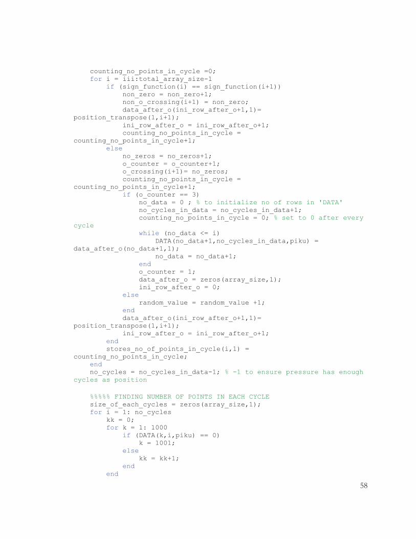
58

counting_no_points_in_cycle =0; for i = iii:total_array_size-1 if (sign_function(i) == sign_function(i+1)) non_zero = non_zero+1; non_o_crossing(i+1) = non_zero; data_after_o(ini_row_after_o+1,1)= position_transpose(1,i+1); ini_row_after_o = ini_row_after_o+1; counting_no_points_in_cycle = counting_no_points_in_cycle+1; else no_zeros = no_zeros+1; o_counter = o_counter+1; o_crossing(i+1)= no_zeros; counting_no_points_in_cycle = counting_no_points_in_cycle+1; if (o_counter == 3) no_data = 0 ; % to initialize no of rows in 'DATA' no_cycles_in_data = no_cycles_in_data+1; counting_no_points_in_cycle = 0; % set to 0 after every cycle while (no_data <= i) DATA(no_data+1,no_cycles_in_data,piku) = data_after_o(no_data+1,1); no_data = no_data+1; end o_counter = 1; data_after_o = zeros(array_size,1); ini_row_after_o = 0; else random_value = random_value +1; end data_after_o(ini_row_after_o+1,1)= position_transpose(1,i+1); ini_row_after_o = ini_row_after_o+1; end stores_no_of_points_in_cycle(i,1) = counting_no_points_in_cycle; end no_cycles = no_cycles_in_data-1; % -1 to ensure pressure has enough cycles as position %%%%% FINDING NUMBER OF POINTS IN EACH CYCLE size_of_each_cycles = zeros(array_size,1); for i = 1: no_cycles kk = 0; for k = 1: 1000 if (DATA(k,i,piku) == 0) k = 1001; else kk = kk+1; end end

59

size_of_each_cycles(i,1) = kk; end minimum_data_points = min(size_of_each_cycles((1:no_cycles),1)); maximum_data_points = max(size_of_each_cycles((1:no_cycles),1)); %%%%% FINDING NUMBER OF CYCLES ACROSS EACH POINT IN ALL CYCLES zero_data = 0; for j = 1:maximum_data_points non_zero_data = 0; for i = 1:no_cycles if(DATA(j,i,piku)==0) zero_data = zero_data+1; else non_zero_data = non_zero_data+1; end end size_of_each_row(j,1)= non_zero_data; end %%% ALLOCATING PRESSURE BASED ON FIRST ZERO dddd = 1; for j = 1:no_cycles for i = 1:1000 %no_points_pressure_cycle PRESSURE(i,j,piku) = pressure(kkkk+dddd,1); %%% 'kkkk' to be used in pressure needs to be WATCHED as.... PRESSURE_A(i,j,piku) = pressure_a(kkkk+dddd,1); %%% it varies when and where 0 crossing occurs PRESSURE_B(i,j,piku) = pressure_b(kkkk+dddd,1); %%% use kkkk value to be about == kkkk = kkkk+1; end end %%%%%%%% POST PROCESSING %%%%%%%% %%%%% AVERAGE IN AN EXPERIMENT for p = 1:maximum_data_points %average across the row average(p,1,piku) = sum(DATA(p,1:no_cycles,piku))/size_of_each_row(p,1); average_pressure_DP(p,1,piku) = sum(PRESSURE(p,1:no_cycles,piku))/no_cycles; average_pressure_a1(p,1,piku)= sum(PRESSURE_A(p,1:no_cycles,piku))/no_cycles; average_pressure_b1(p,1,piku)= sum(PRESSURE_B(p,1:no_cycles,piku))/no_cycles; end avg_length(piku,1) = length(average(:,:,piku)); max_position = max(average(1:maximum_data_points,1)); min_position = min(average(1:maximum_data_points,1)); max_press(1,piku) = abs(max(average_pressure_DP(:,1,piku))); min_press(1,piku) = abs(min(average_pressure_DP(:,1,piku)));

60

avg_press(1,piku) = (max_press(1,piku)+min_press(1,piku))/2; for i = 1:maximum_data_points average_pressure(i,1,piku) = average_pressure_DP(i,1,piku)+(avg_press(1,piku)-max_press(1,piku)); end max_press_a(1,piku) = abs(max(average_pressure_a1(:,1,piku))); min_press_a(1,piku) = abs(min(average_pressure_a1(:,1,piku))); avg_press_a(1,piku) = (max_press_a(1,piku)+min_press_a(1,piku))/2; for i = 1:maximum_data_points average_pressure_a(i,1,piku) = average_pressure_a1(i,1,piku)+(avg_press_a(1,piku)-max_press_a(1,piku)); end max_press_b(1,piku) = abs(max(average_pressure_b1(:,1,piku))); min_press_b(1,piku) = abs(min(average_pressure_b1(:,1,piku))); avg_press_b(1,piku) = (max_press_b(1,piku)+min_press_b(1,piku))/2; for i = 1:maximum_data_points average_pressure_b(i,1,piku) = average_pressure_b1(i,1,piku)+(avg_press_b(1,piku)-max_press_b(1,piku)); end end max_length = max(avg_length(1:N)); min_length = min(avg_length(1:N)); %%%%% AVERAGE ACROSS DIFFERENT EXPERIMENTS %%%%% for p = 1:min_length average_average(p,1) = sum(average(p,1,1:N))/N; average_average_pressure(p,1)= sum(average_pressure(p,1,1:N))/N; end max_avg_position = max(average_average(1:min_length,1)); min_avg_position = min(average_average(1:min_length,1)); max_avg_pressure = max(average_average_pressure(1:min_length,1)); min_avg_pressure = min(average_average_pressure(1:min_length,1)); counter = 0; % to find MAXIMUM average pressure point p = 1; while p < min_length if (average_average_pressure(p,1) == max_avg_pressure) p = min_length + 1; else counter = counter + 1; p = p+1; end end max_avg_pressure_place = counter+1; counter = 0; % to find MINIMUM average pressure point p = 1;

61

while p < min_length if (average_average_pressure(p,1) == min_avg_pressure) p = min_length + 1; else counter = counter + 1; p = p+1; end end min_avg_pressure_place = counter+1; suma = 0; %summation for standard deviation suma_pressure = 0; for i = 1:min_length for piku = 1 : N suma = suma + (average(i,1,piku)-average_average(i,1)).^2; suma_pressure = suma_pressure + (average_pressure(i,1,piku)-average_average_pressure(i,1)).^2; end std_dev(i,1) = (suma/(N-1)).^(0.5); std_dev_pressure(i,1) = (suma_pressure/(N-1)).^(0.5); suma = 0; suma_pressure = 0; var_std_dev(i,1) = (std_dev(i,1)).^2; var_std_dev_pressure(i,1) = (std_dev_pressure(i,1)).^2; end %%% For Coefficient of Variation % for i = 1: N for i=1:min_length COV(i,1) = std_dev_pressure(i,1)/abs(average_average_pressure(i,1)); end std_dev_max_avg_pressure = std_dev_pressure(max_avg_pressure_place,1); std_dev_min_avg_pressure = std_dev_pressure(min_avg_pressure_place,1); %%%%% SINUSOINDAL MOTION %%%%% nu = mu/rho; %m2/s diameter_tube = 2.5e-3; %m length_tube = 0.19; %m area_tubes = pi()/4*(diameter_tube)^2;%m2 diameter_piston = 5e-2; %m area_piston = pi()/4*(diameter_piston)^2;%m2 omega_curve = 2*pi()*frequency_curve; % valensi_number = omega*(diameter_tube)^2/(4*nu); amplitude = max_avg_position; % the maximum position it sees (CHECK FOR MINUS OR PLUS based on how position starts time = 1/(frequency_curve); % time required for a cycle % for one cycle: sine_position(1:maximum_data_points)= amplitude*sin(2*pi()*frequency_curve*(0:time/(maximum_data_points-1):time));

62

cosine_velocity(1:maximum_data_points)= amplitude*omega_curve*cos(2*pi()*frequency_curve*(0:time/(maximum_data_points-1):time)); sine_mass_flow_rate(1:maximum_data_points)= rho*cosine_velocity(1:maximum_data_points)*area_piston; sine_velocity_air(1:maximum_data_points) = sine_mass_flow_rate(1:maximum_data_points)/(rho*area_tubes*no_tubes)/1000; % /1000 for mm to m max_sine_vel_air = max(abs(sine_velocity_air(1:maximum_data_points))); min_sine_vel_air = min(abs(sine_velocity_air(1:maximum_data_points))); aaa = 0:time/(maximum_data_points-1):time; %(finds 1000 points from 0 to time for a cycle) bbb = aaa'; size_of_row_in_data_series = maximum_data_points; time_for_a_cycle = aaa; %%%%% For velocity, Re, and cf %%% using v = x*w*cost(wt) min_vel_limit = 0.01; for i = 1:size_of_row_in_data_series velocity_piston(i,1) = (average(i,1)/1000)*omega_curve*cos(omega_curve*aaa(1,i)*pi()/180); % *pi/180 to convert degree to radian % if (velocity_piston(i,1) <= min_vel_limit) % if (velocity_piston(i,1) >= -min_vel_limit) % velocity_piston(i,1) = 0; % else % velocity_piston(i,1)=velocity_piston(i,1); % end % else % velocity_piston(i,1)=velocity_piston(i,1); % end mass_flow_rate(i,1)= rho*velocity_piston(i,1)*area_piston; velocity_air(i,1) = mass_flow_rate(i,1)/(rho*area_tubes*no_tubes); Re_d(i,1) = rho*diameter_tube*abs(velocity_air(i,1))/mu; cf(i,1) = abs(average_pressure(i,1))*diameter_tube/(1/2*rho*(velocity_air(i,1)).^2*length_tube); end max_re = max(Re_d(1:size_of_row_in_data_series)); max_cf = max(cf(1:size_of_row_in_data_series)); max_vel_piston = max(abs(velocity_piston(1:size_of_row_in_data_series))); max_vel_air = max(abs(velocity_air(1:size_of_row_in_data_series))); max_mass = max(mass_flow_rate(1:size_of_row_in_data_series)); min_re = min(Re_d(1:size_of_row_in_data_series)); min_cf = min(cf(1:size_of_row_in_data_series)); min_vel_piston = min(abs(velocity_piston(1:size_of_row_in_data_series))); min_vel_air = min(abs(velocity_air(1:size_of_row_in_data_series))); min_mass = min(mass_flow_rate(1:size_of_row_in_data_series));

63

figure yyaxis left plot(aaa,average(1:size_of_row_in_data_series,1),'b','LineWidth',1.5); set(gca, 'FontSize', 25) xlabel('Time for a cycle (s)') % x-axis label ylabel('Ensemble-averaged Pos (mm)& Velocity (m/s)') % y-axis label hold on yyaxis left plot(aaa,velocity_air(1:size_of_row_in_data_series,1),'r','LineWidth',1.5);%,'LineWidth',1); hold off hold on yyaxis right plot(aaa,average_average_pressure(1:size_of_row_in_data_series,1),'g','LineWidth',1.5); ylabel('Ensemble-averaged Pressure (Pa)') % y-axis label hold off legend ('Position','Velocity of air','Pressure drop'); % aaaa = aaa(1,(1:10:size_of_row_in_data_series)); figure set(gca, 'FontSize', 30) hold on plot(aaa(1,(1:1:size_of_row_in_data_series)),average_average_pressure(1:1:size_of_row_in_data_series,1),'-*b','LineWidth',1.5); hold off hold on plot(aaa(1,(1:10:size_of_row_in_data_series)),dP_CFD,'-*r','LineWidth',1.5);%,'LineWidth',1); hold off xlabel('Time for a cycle (s)') % x-axis label ylabel('Ensemble-averaged Pressure Drop (Pa)') % y-axis label legend ('Experiment' ,'CFD'); figure yyaxis left plot(aaa,sine_position,'r','LineWidth',1.5); set(gca, 'FontSize', 22) xlabel('Time for a cycle (s)') % x-axis label ylabel('Ensemble-averaged Position (mm) & Air Velocity (m/s)') % y-axis label hold on yyaxis left plot(aaa,sine_velocity_air,'b','LineWidth',1.5);%,'LineWidth',1); hold off hold on yyaxis right plot(aaa,average_average_pressure(1:size_of_row_in_data_series,1),'g','LineWidth',1.5); ylabel('Ensemble-averaged Pressure (Pa)') % y-axis label hold off legend ('Position','Velocity of air','Pressure drop'); Re_plot = Re_d(1:10:size_of_row_in_data_series-1);

64

cf_plot = cf(1:10:size_of_row_in_data_series-1); figure plot(Re_plot,cf_plot,'--ro'); hold on plot(Re_CFD,cf_CFD,'--b*'); hold off hold on plot(Re_SAGE,cf_SAGE,'--ks'); hold off set(gca, 'FontSize', 30) xlabel('Reynolds Number (Re)') % x-axis label ylabel('Coefficient of Friction (cf)') % y-axis label ylim([0 2]); legend ('Experimental','CFD','Sage'); %%%%% INDIVIDUAL PRESSURE diff = 1; cccccc= average_pressure_a(1:diff:size_of_row_in_data_series,1); figure plot(aaa(1:diff:size_of_row_in_data_series),average_pressure_a(1:diff:size_of_row_in_data_series),'-o','LineWidth',1.5); set(gca, 'FontSize', 30) xlabel('Time for a cycle (s)') % x-axis label ylabel('Ensemble-averaged Pressure (Pa)') % y-axis label hold on plot(aaa(1:diff:size_of_row_in_data_series),average_pressure_b(1:diff:size_of_row_in_data_series),'-or','LineWidth',1.5);%,'LineWidth',1); hold off hold on plot(aaa(1:diff:size_of_row_in_data_series),average_pressure(1:diff:size_of_row_in_data_series),'-og','LineWidth',1.5); hold off legend ('Pressure at Sensor 1','Pressure at Sensor 2','Pressure drop'); diff = 200; figure plot(time_pressure(1:diff:total_array_size),pressure_a(1:diff:total_array_size),'-o','LineWidth',1.5); set(gca, 'FontSize', 27) xlabel('Total time (s)') % x-axis label ylabel('Pressure in the system (Pa)') % y-axis label hold on plot(time_pressure(1:diff:total_array_size),pressure_b(1:diff:total_array_size),'-or','LineWidth',1.5); hold off hold on plot(time_pressure(1:diff:total_array_size),pressure(1:diff:total_array_size),'-og','LineWidth',1.5); hold off legend ('Pressure at Sensor 1','Pressure at Sensor 2','Pressure Drop'); % figure

65

plot(aaa,average_average_pressure(1:size_of_row_in_data_series,1),'r','LineWidth',1.5); hold on plot(aaa,average_pressure(1:size_of_row_in_data_series,1,1),'g','LineWidth',1.5); hold off % hold on % plot(aaa,COV,'k','LineWidth',1.5); % hold off set(gca, 'FontSize', 27) xlabel('Time for a cycle (s)') % x-axis label ylabel('Ensemble-averaged Pressure Drop (Pa)') % y-axis label legend ('Average of 11 experiments' ,'Average of an experiment');%, 'COV'); figure plot(average_average_pressure,COV,'ok','LineWidth',1.5); % plot(aaa, COV,'ok','LineWidth',1.5); % hold on % plot(aaa,std_dev_pressure,'+b','LineWidth',1.5); % hold off % hold on % plot(aaa,average_average_pressure,'hg','LineWidth',1.5); % hold off set(gca, 'FontSize', 27) % xlabel('Time for a cycle (s)') % x-axis label xlabel('Ensembled-averaged Pressure Drop (Pa)') % x-axis label ylabel('Coefficient of Variation') % y-axis label legend ('COV');%,'Standard Deviation','Average of 11 experiments'); diff = 1; figure yyaxis left plot(aaa,average(1:size_of_row_in_data_series,1),'b','LineWidth',1.5); set(gca, 'FontSize', 25) % xlabel('Time for a cycle (s)') % x-axis label ylabel('Ensemble-averaged Pos (mm)& Velocity (m/s)') % y-axis label hold on yyaxis left plot(aaa,velocity_air(1:size_of_row_in_data_series,1),'r','LineWidth',1.5);%,'LineWidth',1); hold off hold on yyaxis right % plot(aaa,average_pressure(1:size_of_row_in_data_series,1),'g','LineWidth',1.5); % ylabel('Ensemble-averaged Pressure (Pa)') % y-axis label % hold off % legend ('Position','Velocity of air','Pressure drop'); plot(aaa(1:diff:size_of_row_in_data_series),average_pressure_a(1:diff:size_of_row_in_data_series),'-og','LineWidth',1.5); set(gca, 'FontSize', 30) xlabel('Time for a cycle (s)') % x-axis label

66

ylabel('Ensemble-averaged Pressure (Pa)') % y-axis label hold on plot(aaa(1:diff:size_of_row_in_data_series),average_pressure_b(1:diff:size_of_row_in_data_series),'-or','LineWidth',1.5);%,'LineWidth',1); hold off hold on plot(aaa(1:diff:size_of_row_in_data_series),average_pressure(1:diff:size_of_row_in_data_series),'-ok','LineWidth',1.5); hold off legend ('Position','Velocity of air','Pressure at Sensor 1','Pressure at Sensor 2'); curve_fit_cf=-7.387e-6*RE_max_exp+0.1524; figure plot(RE_max_exp,cf_max_exp,'r^','markersize',15,'LineWidth',1.5); hold on plot(RE_max_exp,curve_fit_cf,'-k','markersize',15,'LineWidth',1.5); hold off hold on plot(RE_max_exp,cf_turb,'--b*','markersize',15,'LineWidth',1.5); hold off set(gca, 'FontSize', 30) xlabel('Reynolds Number (Re_{max})') % x-axis label ylabel('Coefficient of Friction (C_{f})') % y-axis label ylim([0 0.14]); legend ('Experimental C_{f}','Curve-fit Experimental C_{f}','Theoretical C_{f}');