design and evaluation of an emg-based recording and ... · pdf filetwo ways of detecting the...

Project Thesis

Design and Evaluation of an EMG-based

Recording and Detection System

Clemens Amon

submitted to theInstitute of Electronic Music and Acoustics

of theUniversity of Music and Performing Arts Graz

in June 2013

Supervisor:MSc Ph.D. Georgios Marentakis

institute of electronic music and acoustics

ii

Abstract

The project investigates the usability of muscle contractions detected by surface elec-tromyography (EMG) sensors as an input channel for the gestural or subtle control ofelectric devices. A wearable hardware prototype is presented that consists of a sensorstrap and a signal conditioning (amplification and filtering) unit. Signal detection tech-niques are discussed and an evaluation framework is presented based on signal detectiontheory. Using the framework common envelope tracking techniques are compared in auser study that uses the prototype. This work forms the basis for further research onusing EMG signals for controlling, regulation, and navigation purposes as well as musicperformance.

iii

Zusammenfassung

Das Projekt untersucht die Nutzbarkeit von Muskelkontraktionen, die durch Elektro-myografie-Oberflächensensoren (EMG) abgenommen werden, als Eingangskanal für ge-stische oder feinsinnige Steuerung von elektronischen Geräten. Ein tragbarer Hardware-Prototyp wird vorgestellt, der aus einem Sensorband und einer Einheit zur Signalaufbe-reitung (Verstärkung und Filterung) besteht. Techniken der Signalerkennung werden be-handelt und eine auf der Signalentdeckungstheorie basierende Evaluierungsumgebung wirdpräsentiert. In einer Studie werden bekannte Methoden zur Hüllkurvendetektion verglichenund ausgewertet. Diese Arbeit bildet eine Grundlage für weiterführende Untersuchungenim Bereich der Steuerung, Regelung und Navigation durch EMG-Signale, aber auch dieGrundlage für die Integration von EMG-Signalen in musikalischen Aufführungen.

iv

Contents

1 Introduction 1

1.1 Motivation . . . . . . . . . . . . . . . . . . . . . . . . . . . . . . . . . . . . . 1

1.2 Background . . . . . . . . . . . . . . . . . . . . . . . . . . . . . . . . . . . . 1

1.3 Outline . . . . . . . . . . . . . . . . . . . . . . . . . . . . . . . . . . . . . . . 2

2 Basic of Electromyography 3

2.1 Physiology . . . . . . . . . . . . . . . . . . . . . . . . . . . . . . . . . . . . . 3

2.1.1 Myoelectric Signals . . . . . . . . . . . . . . . . . . . . . . . . . . . . 3

2.1.2 Superposition of the Action Potentials . . . . . . . . . . . . . . . . . . 3

2.2 Sensing and Positioning . . . . . . . . . . . . . . . . . . . . . . . . . . . . . . 5

2.2.1 The EMG Signal . . . . . . . . . . . . . . . . . . . . . . . . . . . . . . 6

2.3 Amplification . . . . . . . . . . . . . . . . . . . . . . . . . . . . . . . . . . . . 10

2.4 Noise and interferences affecting EMG signal . . . . . . . . . . . . . . . . . . . 10

2.5 Signal Processing . . . . . . . . . . . . . . . . . . . . . . . . . . . . . . . . . 11

3 Hardware Implementation 13

3.1 Approach in Concept and Design . . . . . . . . . . . . . . . . . . . . . . . . . 13

3.2 Development and Implementation . . . . . . . . . . . . . . . . . . . . . . . . . 14

3.2.1 Sensor Unit . . . . . . . . . . . . . . . . . . . . . . . . . . . . . . . . 14

3.2.2 Amplification and Filter Unit (AFU) . . . . . . . . . . . . . . . . . . . 15

3.3 Reliability, Annoyances - Discussion . . . . . . . . . . . . . . . . . . . . . . . . 20

4 Theory in EMG Signal Processing 21

4.1 Notch and band-pass filtering . . . . . . . . . . . . . . . . . . . . . . . . . . . 21

4.2 Rectification and Smoothing . . . . . . . . . . . . . . . . . . . . . . . . . . . 23

4.3 Signal Detection Theory . . . . . . . . . . . . . . . . . . . . . . . . . . . . . . 26

4.3.1 Probability Density Function (PDF) . . . . . . . . . . . . . . . . . . . 26

4.3.2 Receiver Operating Characteristics . . . . . . . . . . . . . . . . . . . . 28

4.3.3 Double Threshold Detection . . . . . . . . . . . . . . . . . . . . . . . 29

v

5 Evaluation 32

5.1 User Study . . . . . . . . . . . . . . . . . . . . . . . . . . . . . . . . . . . . . 32

5.1.1 Test 1 . . . . . . . . . . . . . . . . . . . . . . . . . . . . . . . . . . . 32

5.1.2 Test 2a . . . . . . . . . . . . . . . . . . . . . . . . . . . . . . . . . . . 32

5.1.3 Test 2b . . . . . . . . . . . . . . . . . . . . . . . . . . . . . . . . . . . 32

5.2 Evaluation Results . . . . . . . . . . . . . . . . . . . . . . . . . . . . . . . . . 33

6 Conclusion 43

6.1 The live scenario . . . . . . . . . . . . . . . . . . . . . . . . . . . . . . . . . . 43

6.2 Possible Enhancements . . . . . . . . . . . . . . . . . . . . . . . . . . . . . . 44

6.2.1 Hardware . . . . . . . . . . . . . . . . . . . . . . . . . . . . . . . . . . 44

6.2.2 Software . . . . . . . . . . . . . . . . . . . . . . . . . . . . . . . . . . 44

A Additional user study recordings 47

B Discrete amplifier test setup 47

C Printed circuit board layout 48

C.1 List of Parts . . . . . . . . . . . . . . . . . . . . . . . . . . . . . . . . . . . . 49

1

1 Introduction

1.1 Motivation

In the last years gesture interaction between humans and computers became more important.This is because there is an increased need for subtle control systems which makes myoelectricsignals interesting. In particular in the field of computer music such signals are valuable as theycan be used to augment a musical or dancing performance. In this project, Electromyography(EMG) signals are processed and detected and an interface is designed and evaluated in acontrol setting.

1.2 Background

The idea of using EMG for system control is not new. In 1990 Knapp and Lusted introduced"Biomuse" a bioelectric controller for computer music applications [RBK90]. This system con-sists of two separate components. A bioelectric interface and a signal processing unit. Thebioelectric interface consists of electrodes and sensors that are placed on the user’s body, whichsense Electromyography (EMG) , Electroencephalography (EEG) i.e. the brain’s electrical ac-tivity, and EOG (Electrooculography) i.e. eye movement activity. The incoming signals areconnected to a patchbox and are then processed in the signal processing unit. There the signalsare digital-analog converted, filtered and analysed by a digital signal processing (DSP) chip.The unit analyses all input signals in real-time and receives and sends information to a hostcomputer over a standard RS-232 serial interface. In addition, it receives and sends MIDI in-formation. The Biomuse can be used to control synthesizers, sequencers, drum machines, orany other MIDI device.Tanaka also used bioelectric signals to realize interaction in the context of music perfor-mance [TKA02]. Tanaka describes a system where EMG is combined with relative positionsensing to overcome the inability of EMG to measure isotonic movements. EMG measuresmuscle activity without motion (isometric) very well, but motion without change in tension(isotonic) relatively poorly. Like in the "Biomuse" project, the aim was to create multimodalinteraction to increase the number of inputs to the control system and consequently the numberof independent parameters that define the interaction.Costanza, Inverso and Allen proposed in [CIA05] and [CIAM07] another approach of using EMGsignals for control purposes. Here, the bioelectrical signals were used to create interfaces thatallow subtle and minimal mobile interaction, without disruption of the surrounding environment.Using a wireless EMG device, subjects performed walking tasks while making contractions ofdifferent durations. These motionless gestures were sensed and detected online. An actionwas triggered if the signal exceeded a certain threshold for a predefined time. Costanza et al.showed that EMG can be used successfully as a controller. Using their detection method thecontraction needs to be finished in order to be analysed. So time exact triggering is difficult to

Introduction 2

realise.In [NKV+] hand gestures were identified by analysing a four-channel EMG with independentcomponent analysis (ICA), where a signal is decomposed in their independent components.This method is used in bio-signal applications to isolate signals from different muscles andanalyse them individually. Human hand gestures are used very often in non verbal interactionsamong people. Thus their interpretation in human computer interaction (HCI) will be a moreinteresting, especially in cases in which no physically controller (like a computer mouse, or anypointing device) is available or the use of a controller is not wanted.Advances in integrated circuit technology allow the inclusion of high sensitivity low noise am-plifiers in embedded, battery operated, devices at low cost. This enables the construction ofsmall, wearable, intimate devices, that can be used to controlling musical instruments, in thefield of rehabilitaion engineering, and in the design of intimate interactions. In nearly all pre-vious works, in which EMG was used, the amplitude envelope of the EMG was extracted viaa straightforward RMS calculation. Beyond that more parameters like median frequency canbe extracted out of the signal to achieve more degrees of control for the user and to openpossibilities for the creation of new sounds and new ways of controlling them.

1.3 Outline

This report starts by providing the physiological and technical background on EMG signalacquisition (section 2) and then describes in detail the EMG signal and its acquisition andprocessing. The development of an EMG hardware device (section 3) is then presented and asoftware implementation of signal filtering and amplitude extraction is introduced (section 2.5).Two ways of detecting the digital EMG signal and their realisation in MATLAB are presentedin sections 4.3 and 4.3.3. In section 5.1 the results of an user study are presented wherethe introduced methods are tested and analysed and evaluated using signal detection theory(section 5). An application for using this system in a live and real-time environment is designed(section 6.1).

Institute for Electronic Music and Acoustics Graz

3

2 Basic of Electromyography

2.1 Physiology

2.1.1 Myoelectric Signals

Myoelectric signals are measurable signals which appear during muscle activation. Duringmuscle contraction, small electrical currents are generated by the exchange of ions acrossmuscle fiber membranes [Win99, 26]. There are two types of EMG: surface electromyography(SEMG, non-invasive) and needle electromyography (NEMG, invasive). Surface EMG recordsmuscle activity on the skin surface that surrounds a muscle. Electrodes are attached to the skinand provide a crude assessment of the muscle activity below. SEMG provides information onthe onset time, duration and relative intensity of muscle activation. While an electrode is placedover the muscle on the skin in SEMG, a needle inserted through the skin into the muscle is usedin needle EMG. Needle EMG is more accurate and is therefore preferred in medical diagnosticsfor the assessment of muscle disease or ongoing pathology [JER]. Invasive needle electrodesacquire signals better and can access individual muscle fibres. In surface EMG the signal is acomposite of all the muscle fiber action potentials occurring in the muscles underlying the skin.Intra-muscular recordings can be painful and have only medical applications. Surface electrodesdo not inflict pain to the user and for this reason they are preferred in HCI and are used inthis project to acquire muscle activity in satisfactory quality, as we will see later. There aretwo types of SEMG electrodes: wet and dry SEMG electrodes. SEMG electrodes are appliedto the skin using conductive gel as an intermediate layer to ensure good conductivity betweenthe skin and the electrode. It is recommended to clean the skin before placing the electrodesusing either rubbing alcohol or a special skin preparation fluid for SEMG.

2.1.2 Superposition of the Action Potentials

The nervous system controls muscle contraction by activating discrete motor units and thecorresponding muscle fibers at variable firing rates. The number of muscle fibers within eachunit can vary. The activation of a motor unit leads to the activation of all its muscle fibers.Muscle tissue conducts electrical potentials similar to the way nerves do. These are called muscleaction potentials (MAP). The combination of the muscle fiber action potentials from all themuscle fibers of a single motor unit yields the motor unit action potential (MUAP) [BJ85]. Thisis the linear sum of all active motor units. Figure 2.1 shows the structure and the producedtension of the motor units and its corresponding muscle fibres.

Basic of Electromyography 4

Figure 2.1: Structure of the motor units and the tension when a singleor more motor units are activated [Dis11]


5

2.2 Sensing and Positioning

A muscle contraction does not give rise to a single MUAP, but results in MUAP sequencesfrom different motor units, whose superposition is the acquired EMG signal. The amplitude ofeach single MUAP depends on the distance of the firing motor unit to the electrode and thefilter characteristics of the tissue. A higher distance to the electrode leads to a decrease in theamplitude. Figure 2.2 shows a simplified illustration of the superposition of action potentialsfrom different motor acquired with needle EMG.

Figure 2.2: Superposition of MUAPs [Kon05, 8]: Three motor unitseach firing one single MUAP. The fist motor unit consists ofthree muscle fibres and the second and the third motor unitconsists of four muscle fibres. The superposition is recordedwith a needle electrode. Due to the filter characteristics ofthe tissue the amplitude of the single impulses of the musclefibres with a greater distance to the electrode are smallerthan the amplitude of the impulses of the muscle fibres closeto the electrode.

MUAP sequences are specified by two values: The firing rate FF

, and the inter-pulse intervals(IPI). F

F

describes the number of discharges over a certain time period, and is measured inHertz (Hz). More demonstratively the firing rate is usually specified in the SI1 base unit s-1. Theinter-pulse intervals (IPI) T

F

is a list of periods between successive MUAPs. The instantaneousfiring rate is obtained by inverting T

F

. The discharge properties are stochastic. Instead of dis-charging APs with a constant inter-pulse interval, the timing of successive APs fluctuates. Most

1 Abbr. for fr.: Le Système international d’unités, International System of Units


studies indicate that the minimum firing or firing rate is between 5 and 7 s-1. The highest initialrate of discharge varies among studies, but commonly ranges between 12 and 26 s-1 [Win99, 26].

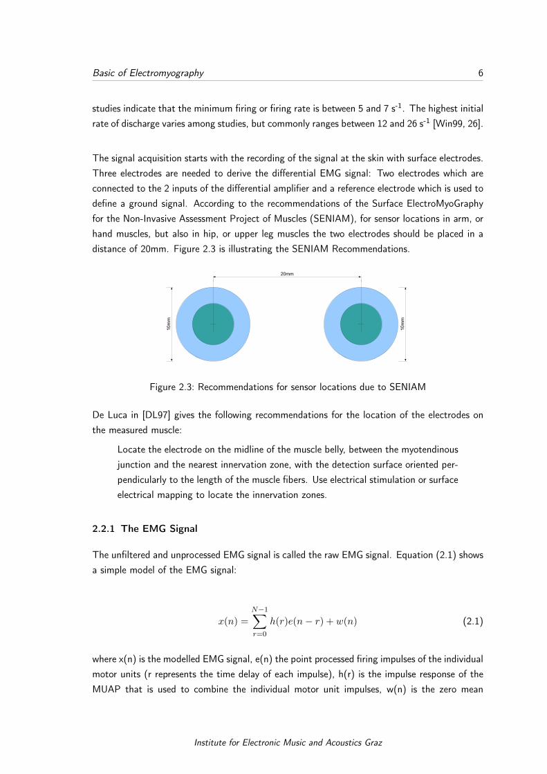
The signal acquisition starts with the recording of the signal at the skin with surface electrodes.Three electrodes are needed to derive the differential EMG signal: Two electrodes which areconnected to the 2 inputs of the differential amplifier and a reference electrode which is used todefine a ground signal. According to the recommendations of the Surface ElectroMyoGraphyfor the Non-Invasive Assessment Project of Muscles (SENIAM), for sensor locations in arm, orhand muscles, but also in hip, or upper leg muscles the two electrodes should be placed in adistance of 20mm. Figure 2.3 is illustrating the SENIAM Recommendations.

Figure 2.3: Recommendations for sensor locations due to SENIAM

De Luca in [DL97] gives the following recommendations for the location of the electrodes onthe measured muscle:

Locate the electrode on the midline of the muscle belly, between the myotendinousjunction and the nearest innervation zone, with the detection surface oriented per-pendicularly to the length of the muscle fibers. Use electrical stimulation or surfaceelectrical mapping to locate the innervation zones.

2.2.1 The EMG Signal

The unfiltered and unprocessed EMG signal is called the raw EMG signal. Equation (2.1) showsa simple model of the EMG signal:

x(n) =N�1X

r=0

h(r)e(n� r) + w(n) (2.1)

where x(n) is the modelled EMG signal, e(n) the point processed firing impulses of the individualmotor units (r represents the time delay of each impulse), h(r) is the impulse response of theMUAP that is used to combine the individual motor unit impulses, w(n) is the zero mean



addictive white Gaussian noise, and N is the number of motor unit firings. This model showsthe response of the system, here the MUAP, to a series of delayed impulses and is not regardingthe filtering characteristics of the tissue.

Figure 2.4 shows a raw EMG Signal of a sequence of dynamic contractions and the noisewithout muscle activity recorded with BETTERWITTS surface electrodes placed at extensormale. When the muscle is relaxed the noise floor can be seen. The noise depends on manyfactors that affect signal quality: the amplifier specification and its common mode rejectionratio (CMRR), the quality of the surface electrodes, the way the setup is realized (i.e. thenumber of electrodes used), and the quality of the cables used (shielded or unshielded) used,and movement artifacts that can occur during recording (i.e. when the cables are not fixed).

0 0.5 1 1.5 2 2.5 3 3.5 4 4.5 5 5.5!1

!0.8

!0.6

!0.4

!0.2

0

0.2

0.4

0.6

0.8

1

EMG signal ! extensor contraction ! raw signal ! waveform

Time in seconds

Am

plit

ud

e

Figure 2.4: EMG Signal and Noise in the time domain

In figure 2.5, the frequency response of the raw EMG signal of a static contraction of extensormale and the frequency response of the noise recorded at extensor male without voluntarymuscle activity is shown. A strong 50 Hz power line interference can be seen in the noisefigure. Figure 2.6 shows the power spectrum of a short and a long contraction of musculusextensor male with a window size of 200 ms (8820 samples at sample rate of 44.1 kHz). Thegreen and blue ranges mark the signal used for the fft plot. It can be seen that the usefulfrequency range of the signal extends between 20 Hz and 500 Hz, while most of the energy isdistributed from 50 Hz to 400 Hz.



0 100 200 300 400 500 600 700 800 900 10000

0.5

1

1.5

2

2.5

3

3.5

4x 10

!7 EMG signal ! extensor noise ! raw signal ! frequency (fft ! lin)

Frequency in Hz

Magnitu

de

0 100 200 300 400 500 600 700 800 900 10000

1

2

3

4

5

6

7x 10

!6 EMG signal ! extensor contraction ! raw signal ! frequency (fft ! lin)

Frequency in Hz

Magnitu

de

Figure 2.5: EMG Signal and Noise in the frequency domain



0 0.5 1 1.5 2 2.5 3 3.5 4 4.5 5 5.5!1

!0.5

0

0.5

1EMG Signal ! Extensor!contraction ! betterwitts ! raw signal ! waveform

Time in seconds / the green and blue areas show the windows used for fft below

Am

plit

ud

e

0 100 200 300 400 500 600 700 800 900 10000

0.5

1

1.5

2x 10

!5 EMG Signal ! Extensor!contraction ! betterwitts ! raw signal ! short contraction ! frequency (fft ! lin) ! win: green area

Frequency in Hz

Ma

gn

itud

e

0 100 200 300 400 500 600 700 800 900 10000

2

4

6

8x 10

!6 EMG Signal ! Extensor!contraction ! betterwitts ! raw signal ! long contraction ! frequency (fft ! lin) ! win: blue area

Frequency in Hz

Ma

gn

itud

e

Figure 2.6: (1) raw time signal with fft window marked, (2) powerspectrum of a short contraction, (3) power spectrum of along contraction



2.3 Amplification

The amplitude of the superimposed MUAPs is very small (0 to 10 mV) and needs to be amplified.Since the difference of the two electrodes is amplified, it is important that the amplifier has ahigh Common Mode Rejection Ratio (CMRR> 90dB). The CMRR describes the accuracy withwhich a differential amplifier rejects common input, i.e. subtracts one input from the other,relative to the gain with which the difference in its inputs is amplified. The CMRR is measured inDecibel (dB). To achieve the necessary gain factor a multi-stage amplification design is needed.Typically a differential amplifier is used in the first stage [RHMY06]. In the second stage anactive inverting operational amplifier is used to get the desired signal amplitude. Before beinganalog to digital converted and processed, the signal can be filtered to eliminate low-frequencyor high-frequency noise, or other possible artifacts. The block diagram of a basic EMG sensorand amplification system is shown in figure 2.7.

Figure 2.7: Block diagram of an EMG sensor and amplification network

2.4 Noise and interferences affecting EMG signal

Two main issues influence the fidelity of the signal. The first is the signal-to-noise ratio (SNR),that is the ratio of the energy in the EMG signals to the energy in the noise signal. In general,noise is defined as electrical signals that are not part of the desired EMG signal. The power lineradiation (50 Hz) is a common source of noise in the field of EMG. The second is the distortion ofthe signal waveform caused by filtering, meaning that the relative contribution of any frequencycomponent in the EMG signal should not be altered to avoid phase shifts [RHMY06]. Thereforethe use of analog and digital infinite impulse response (IIR) filters should be minimized, as thesefilters may introduce frequency-dependent phase shifts in the EMG signal. This can result inincreased response onset latency and distortion of the input waveform. If filtering is desired,any detecting and recording device should process the signal linearly. E.g. in [Luc02] De Lucarecommends to avoid the implementation of a 50 Hz notch filter when there are alternativemethods of dealing with the power line radiation. Symmetrical digital finite impulse response(FIR) filters do not cause phase shifts. In contrast to single user live scenarios, where latencyshould be avoided, in within-participants designs phase shifts and the accompanying increasedlatencies are less problematic because they are consistent across experimental conditions. As



the distortion of the signal waveform must be kept low, an analog filter with linear phase shift(a Bessel type filter), which does induce a time shift but produces minimum signal distortioncan be applied [BCF+05].

Raez et al. [RHMY06] categorizes the electrical noise, which will interfere with the EMG signalsinto the following types:

1. Inherent noise in electronics equipment: All electronics equipment generate noise. Thisnoise cannot be eliminated; using high quality electronic components can only reduce it.

2. Ambient noise: Electromagnetic radiation is the source of this kind of noise. The surfacesof our bodies are constantly inundated with electric-magnetic radiation and it is virtuallyimpossible to avoid exposure to it on the surface of earth. The ambient noise may haveamplitude that is one to three orders of magnitude greater than the EMG signal.

3. Motion artifacts: Motion artifacts cause irregularities in the data. There are two mainsources for motion artifacts: 1) electrode interface and 2) electrode cable. Motion arti-facts can be reduced by proper design of the electronics circuitry and set-up.

4. Inherent instability of signal: The EMG signal is stochastic in nature. EMG signal isaffected by the firing rate of the motor units, which, in most conditions, fire in thefrequency region of 0 to 20 Hz. This kind of noise is considered as unwanted and theremoval of the noise is important.

2.5 Signal Processing

As mentioned before, the useful frequency range is between 0 Hz and 500 Hz. So filteringthe raw signal is recommended to limit the signal’s frequency range to the desired range. VanBoxtel in [vB08] found that a band-pass frequency range of 20 Hz to 500 Hz appeared to beadequate because there was a negligible contribution of higher frequency components to theEMG signal. In [CJDLR10] De Luca et al. are recommending to set the low-pass filter cornerfrequency to 400 - 450 Hz, where the high end of the SEMG frequency spectrum is expected.Various recommendations for the high-pass filter corner frequency can be found in literature. Allthe recommendations are between 5 Hz and 20 Hz. SENIAM recommends to set the high-passfilter corner frequency to 10 - 20Hz.

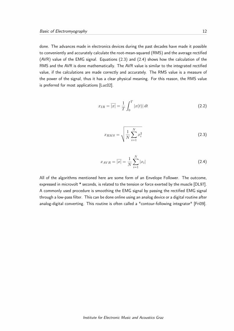
For several decades it has been commonly accepted that the preferred manner for processingthe EMG signal after filtering was to calculate the integrated rectified signal. This was doneby full-wave rectifying the EMG signal, integrating the signal over a specified interval of timeand subsequently forming a time series of the integrated values. Full-wave rectification meansthe conversion of the input waveform to one of constant polarity (positive or negative) at itsoutput. This approach of rectifying and integrating became widespread since it is possible tomake these calculations accurately and inexpensively with the limited electronics technology ofearlier decades. Equation (2.2) shows how the calculation of the integrated rectified signal is



done. The advances made in electronics devices during the past decades have made it possibleto conveniently and accurately calculate the root-mean-squared (RMS) and the average rectified(AVR) value of the EMG signal. Equations (2.3) and (2.4) shows how the calculation of theRMS and the AVR is done mathematically. The AVR value is similar to the integrated rectifiedvalue, if the calculations are made correctly and accurately. The RMS value is a measure ofthe power of the signal, thus it has a clear physical meaning. For this reason, the RMS valueis preferred for most applications [Luc02].

xIR

= |x| = 1

T

ZT

0|x(t)| dt (2.2)

xRMS

=

vuut 1

N

NX

i=1

x2i

(2.3)

xAV R

= |x| = 1

N

NX

i=1

|xi

| (2.4)

All of the algorithms mentioned here are some form of an Envelope Follower. The outcome,expressed in microvolt * seconds, is related to the tension or force exerted by the muscle [DL97].A commonly used procedure is smoothing the EMG signal by passing the rectified EMG signalthrough a low-pass filter. This can be done online using an analog device or a digital routine afteranalog-digital converting. This routine is often called a "contour-following integrator" [Fri09].


Hardware Implementation 13

3 Hardware Implementation

3.1 Approach in Concept and Design

The system proposed in this work is detecting SEMG signals using wet, reusable electrodes withconductive gel placed on the muscle. To make it easier to apply and remove the electrodes,these are integrated into a elastic VELCRO strap similar to the strap Knapp and Lusted usedin their "Biomuse" project in 1990 [RBK90].

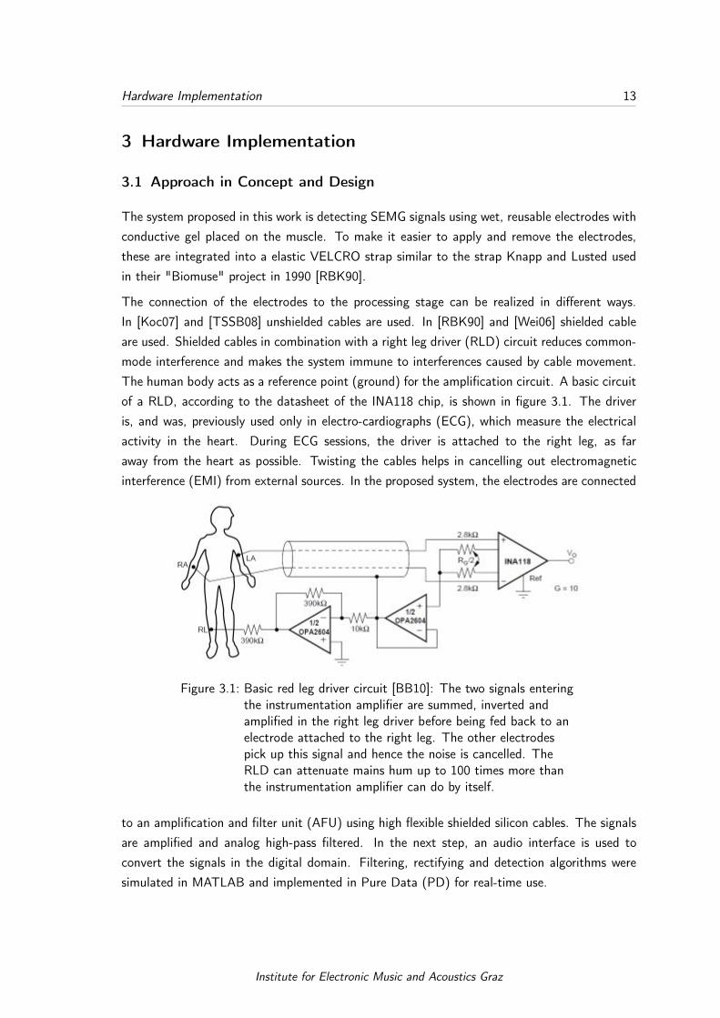
The connection of the electrodes to the processing stage can be realized in different ways.In [Koc07] and [TSSB08] unshielded cables are used. In [RBK90] and [Wei06] shielded cableare used. Shielded cables in combination with a right leg driver (RLD) circuit reduces common-mode interference and makes the system immune to interferences caused by cable movement.The human body acts as a reference point (ground) for the amplification circuit. A basic circuitof a RLD, according to the datasheet of the INA118 chip, is shown in figure 3.1. The driveris, and was, previously used only in electro-cardiographs (ECG), which measure the electricalactivity in the heart. During ECG sessions, the driver is attached to the right leg, as faraway from the heart as possible. Twisting the cables helps in cancelling out electromagneticinterference (EMI) from external sources. In the proposed system, the electrodes are connected

Figure 3.1: Basic red leg driver circuit [BB10]: The two signals enteringthe instrumentation amplifier are summed, inverted andamplified in the right leg driver before being fed back to anelectrode attached to the right leg. The other electrodespick up this signal and hence the noise is cancelled. TheRLD can attenuate mains hum up to 100 times more thanthe instrumentation amplifier can do by itself.

to an amplification and filter unit (AFU) using high flexible shielded silicon cables. The signalsare amplified and analog high-pass filtered. In the next step, an audio interface is used toconvert the signals in the digital domain. Filtering, rectifying and detection algorithms weresimulated in MATLAB and implemented in Pure Data (PD) for real-time use.



Therefore different tasks and scenarios were developed and applications for artificial and musicinteraction were designed. In [CIA05], [TKA02] and [GD] the electrodes, the processing andthe transmitting unit are combined and placed directly at the recorded muscle. The controlsignals are transmitted via bluetooth. In contrast to the work of Costanza et al. [CIA05]and [CIAM07] not especially subtle but apparent movements should be detected in this project.When performing with this system on stage the body movements should refer to the producedand sampled sounds.

3.2 Development and Implementation

3.2.1 Sensor Unit

Figure 3.2: The different electrode types that were tested. From left toright: Disposable self-adhesive Skintact wet electrodes,Betterwits reusable electrodes (gel must be applied on thesurface), Bio-Sense cup electrodes (gel is used to fill thecavity)

Twisted shielded cables are used for the two input electrodes, to minimise interference causedby cable movements. The reference electrode need not be shielded. Instead of using disposablewet electrodes, three reusable electrodes mounted on a VELCRO strap are used. To achievea clean signal, a proper skin preparation using skin preparation gel is recommended as well asusing conductive gel between the skin and the electrodes.

Different disposable and reusable, self and non-adhesive EMG and ECG (electrocardiogram)electrodes were tested (see figure 3.2) relating to their user friendliness and the achieved signalquality. Reusable Non-adhesive Ag/AgCl snap-on EMG electrodes by BETTERWITTS werechosen. Low intrinsic noise in the electrodes and a good integration in the VELCRO strapprovide optimum signal when acquiring data.



3.2.2 Amplification and Filter Unit (AFU)

The developed circuit is based on the principal bio sensor circuit with right leg driver shown infigure 3.1. It is shown in figure 3.3.

B

F

E

C D

A

Figure 3.3: Schematics of "EMG Machine"

To achieve the power supply voltage of +/- 9 V two 9 V transistor batteries were used. Thepositive pole of one battery was connected to the negative pole of the other battery. Thisresults in a virtual ground, and a positive, and a negative 9V pole (see figure 3.3A). Thesecond part of the circuit consists of an integrated circuit (IC) INA118 (see figure 3.3B). It isbuilding the difference between the two input electrodes E1 and E2 and amplifying it by 110.This IC is an instrumentation amplifier whose operation is according to the circuit shown infigure 3.4. This amplifier consists of three operational amplifiers TI082 by Texas Instruments,several resistors R and one gain resistor R

gain

. Equation (3.1) shows the transfer functionof the used instrumentation amplifier design under the precondition R

1

=R2

=R3

=R4

=R. Theinstrumentation amplifier can be divided into two stages, the buffer and the differential amplifierstage.

Vout

= (V1 � V2)(1 +2R

Rgain

) (3.1)

The operational amplifiers OP1 and OP2 in the first stage operate as buffers. This stageprovides a high input impedance, increases the CMRR of the circuit and also enables the buffersto handle much larger common-mode signals without clipping. The two output functions ofthe first stage are shown in equations (3.2) and (3.3).



Figure 3.4: Discrete version of an instrumentation amplifier using TI082operational amplifiers

Vbout1 = V

dif1 = V1(2R

Rgain

+ 1) (3.2)

Vbout2 = V

dif2 = V2(2R

Rgain

+ 1) (3.3)

In the second stage a differential amplifier is amplifying the difference of the two inputs signalsV

1

and V2

. The transfer function of the differential amplifier can be calculated by viewing thiscircuit as a combination of an inverting and a non-inverting operational amplifier. Subfigures5(a) and 5(b) in figure 3.5 show the two circuits.

In the equations (3.4) and (3.5) the output functions of the two amplifiers are presented. Theoutput V

oinv

in equation (3.4) can be derived by driving the first input Vdif1

and setting thesecond input V

dif2

to ground. The output Vononinv

in equation (3.5) can be derived by drivingV

dif2

and setting Vdif1

to ground. Simply adding the two parts results in the output functionof the differential amplifier. See equation (3.6).

Voinv

= �Vdif1

R2

R1(3.4)



(a) (b)

Figure 3.5: The instrumentation amplifier can be seen as a combinationof an (a) inverting and a (b) non-inverting operationalamplifier.

Vononinf

= Vdif2

R1 +R2

R1· R4

R3 +R4(3.5)

Vodif

= Vononinv

+ Voinf

= Vdif2

R1 +R2

R1· R4

R3 +R4� V

dif1R2

R1(3.6)

By choosing R1

= R3

and R2

= R4

you can specify the gain. This can be seen in equation(3.7):

Vodif

=R2

R1· (V

dif2 � Vdif1) (3.7)

By choosing R1

= R2

= R3

= R4

= R the gain of the whole circuit is set to 1. This can beseen in equation (3.8):

Vodif

= Vdif2 � V

dif1 (3.8)

Only the difference gets amplified. It can be seen that for common signals at both inputs Vdif1

and Vdif2

the output Vodif

should be zero. This common mode rejection ratio (CMRR), alsodescribed in section 2.2.1, is useful but not perfect. It depends on the operational amplifierdevice itself and on the matching of the resistor values.



In the AFU the gain of the INA118 is set to 110 by choosing R1=R2=220 ⌦. Equation (3.9)shown how this is calculated:

Gina

= 1 +50k⌦

R1 +R2(3.9)

The INA118 chip has a very high CMRR especially with high gain. A gain of 110 is used inthe AFU which eliminates most noise seen by the cables. Table 3.1 shows an extract of theINA118 data sheet where the CMRR dependent on the gain is listed. A CMRR above 120 dB isobtainable. It’s impossible to completely eliminate motion artifacts in surface electromyographydue to the inherent nature of surface electrodes. The INA118 was integrated in the circuitaccording to figure 3.3B.

Table 3.1: Common-Mode Rejection INA118

PARAMETER CONDITIONS MIN TYP MAX UNITS

Common-Mode Rejection VCM

= ±10V, �RS

= 1kW

G=1 80 90 73 dB

G=10 97 110 89 dB

G = 100 107 120 98 dB

G = 1000 110 125 100 dB

The circuit is complemented by an inverting active high-pass filter with fg

=106Hz and with again of 1.5, see figure 3.3C. This was implemented using a TL082 IC to get rid of movementand surface artifacts, to reduce the 50Hz hum and eliminate any DC offset. Following anotheractive operational amplifier with a gain of 6.6 is used to invert and amplify the signal again andto get a phase of 0 degree, see figure 3.3D. The total gain is now set to 1130. A passive limiterterminates the output voltage to ±0,6V (-5.3dBu) and protects the connected sound card, seefigure 3.3E.

To guarantee a constant ground level and to avoid overswing of voltage an active groundcircuit in combination with a right leg driver (RLD) was used, see figure 3.3F. The right legdriver circuit is realised using an IC OPA2650. This component is often added to biologicalsignal amplifiers to reduce Common-mode interference [Ach11]. See section 2.2.1 for detaileddescription of the RLD. The full schematic and the PCB layout which was designed in CadSoftEAGLE PCB Design Software is illustrated in figure 3.3 and appendix C.1.

A small PCB was designed and etched using the laser printer technique. Figure 3.6 shows thePCB design etched but not drilled yet. The dimensions of the PCB and the housing are listedin the table 3.2. A light and small housing made of plastic was used.



Figure 3.6: Etched printed circuit board, not drilled

Table 3.2: Dimensions: PCB and the housing of the AFU

Dimension AFU

PCB Length 60mm

PCB Width 40mm

PCB Height 3mm

Housing Length 100mm

Housing Width 45mm

Housing Height 30mm


20

The two nine-volt transistor batteries are integrated into the housing. The PCB populated withelectronic components is placed above the batteries. A picture of the integration of the powersupply is shown in figure 7(a). Figure 7(b) shows the built-in populated PCB.

(a) Plastic Housing of "‘EMG-Machine"’ with inte-grated power supply

(b) Plastic Housing of "‘EMG-Machine"’ with inte-grated power supply and populated PCB

3.3 Reliability, Annoyances - Discussion

The three cables that connect the strap to the amplifier and filter unit could cause annoyance.These cables have to be fixed to the body. (e.g.: from the forearm to the upper arm to theshoulder to the side thorax and to the hip or belt where the amplification and filtering unit isfixed). If the cables are fixed properly large movements (like moving the hand around the head)are possible.

Mobile phones close the the cables or to the EMG Machine causes a noticeable hum in thesensor signal and a lower SNR.

Figure 3.7: An illustration of the developed system

Theory in EMG Signal Processing 21

4 Theory in EMG Signal Processing

4.1 Notch and band-pass filtering

The signal is processed using an Infinite Impulse Response (IIR) notch filter that reduce the 50Hz Hum followed by a Finite Impule Response (FIR) band-pass filter to delimit the signal to auseful range and filter out noise in high frequencies. The IIR filter bandwidth is quite narrow(10 Hz) and has a small effect on the signal energy. This filtering is performed in addition tothe one implemented in the hardware device because of its higher order and accordingly higherattenuation and sharper cutoff. Figure 4.1 shows the digitally unfiltered raw signal comparedto the notch and band-pass filtered signal in the frequency domain. A high reduction of the50 Hz component can be seen. The blue range marks the signal portion that is analyzed bythe Fast Fourier Transform (FFT). The analysis window is purposely set to a region where nomuscle activity occurs to show the impact of the filter better. In figure 4.2 the unfiltered andfiltered signal is shown as a spectrogram plot where the hum reduction can also be seen veryclearly. The reduction can also be seen in the decrease of the ripple in the time signal whereno muscle activity is seen (figure 4.3).

0 0.5 1 1.5 2 2.5 3 3.5 4 4.5 5 5.5!1

!0.5

0

0.5

1EMG signal ! extensor ! raw signal ! waveform

Time in s

Am

plit

ude

0 100 200 300 400 500 600 700 800 900 10000

1

2

3x 10

!7 Raw signal (fft ! lin)

Frequency in Hz

Magnitu

de

0 100 200 300 400 500 600 700 800 900 10000

1

2

3x 10

!7 Filtered signal (fft !lin)

Frequency in Hz

Magnitu

de

Figure 4.1: Filtered signal: (1) raw time signal with fft window marked,(2) corresponding fft plot, (3) fft plot of the filtered signal

In the simulation the band-pass filter is realized using one high-pass and one low-pass filter totest different orders and filter types for each filter. The high-pass filter has a cutoff frequency offc

=5 Hz and an order of N=60. The low-pass filter has a cutoff frequency of fc

=400 Hz and anorder of N=10. In the final filtering routine a FIR Butterworth band-pass filter is implementeddue to a lower ripple and a better cut-off frequency behaviour.



Figure 4.2: filtered signal: (1) spectrogram of the raw signal, (2)spectrogram of the notch and band-pass filtered signal

0 0.5 1 1.5!1

!0.5

0

0.5

1EMG Signal ! Extensor!contraction ! betterwitts ! raw signal ! waveform

Time in s

Am

plit

ude

0 0.5 1 1.5!1

!0.5

0

0.5

1EMG Signal ! Extensor!contraction ! betterwitts ! notch/bandbpass filtered signal ! waveform

Time in s

Am

plit

ude

Figure 4.3: Filtered signal: (1) raw time signal, (2) notch and band-passfiltered time signal



4.2 Rectification and Smoothing

As mentioned in section 2.5 the RMS value is preferred for most applications in EMG to esti-mate the amplitude because it reflects the energy of the physiological activities in the motorunit during contraction. In this section, four different methods for rectifying and smoothing thesignal are simulated and implemented in MATLAB. For all following calculations the notch andband-pass filtered signal serves as input signal. Table 4.1 lists the four filter and rectificationmodes proposed in this project. A good combination method should minimize the fluctuationsof the signals amplitude. Figure 4.4 shows a comparison of the four proposed combinations ofrectifying and smoothing algorithms. In the first graph the absolute values (full-wave rectifica-tion, blue) are presented. In graph number two a 10 Hz low-pass filter is applied on the absolutevalues. A well smoothed signal can be achieved using this method. The Hilbert transform offersanother option to rectify and smooth the signal. Equation (4.1) shows how the calculation isdone.

bx(t) = |H {x(t)}| (4.1)

Graph three and four in figure 4.4 show how the raw and the low-pass filtered hilbert transformedsignal looks like the time domain. In figure 4.5 the hilbert transformed signal x(t) is compared tothe rectified signal (full-wave rectification). It can be seen the the Hilbert Transform algorithmacts like a envelope follower and hence as shown in figure 4.6 will give a higher amplitude afterthe low-pass filtering. The hilbert transformed and butterworth low-pass filtered signal with acutoff frequency of f

c

=10 Hz and an order of N=4 is smoothed quite well but shows a smallundershoot. The shape of the filtered full-wave rectified signal is similar to the filtered Hilberttransformed signal.

Table 4.1: Evaluated modes processing the signal

Mode No. Description

1 Absolute values

2 Absolute values + LP filtered [10Hz, IIR, win: BW, filter order n=4]

3 Hilbert

4 Hilbert + LP filtered [10Hz, IIR, win: BW, filter order n=4]



0 0.5 1 1.5 2 2.5 3 3.5 4 4.5 5 5.50

0.5

1

mode 1: EMG Signal ! Extensor!contraction ! betterwitts ! rectified (absolute values)

Time in seconds

Am

plit

ud

e

0 0.5 1 1.5 2 2.5 3 3.5 4 4.5 5 5.50

0.2

0.4

mode 2: EMG Signal ! Extensor!contraction ! betterwitts ! rectified (absolute values) + LP filtered [10Hz, IIR, win: BW, filter order n=4]

Time in seconds

Am

plit

ud

e

0 0.5 1 1.5 2 2.5 3 3.5 4 4.5 5 5.50

0.5

1

mode 3: EMG Signal ! Extensor!contraction ! betterwitts ! hilbert transformed

Time in seconds

Am

plit

ud

e

0 0.5 1 1.5 2 2.5 3 3.5 4 4.5 5 5.50

0.2

0.4

0.6mode 4: EMG Signal ! Extensor!contraction ! betterwitts ! hilbert transformed + LP filtered [10Hz, IIR, win: BW, filter order n=4]

Time in seconds

Am

plit

ud

e

Figure 4.4: (1)mode 1: Absolute values, (2) mode 2: Absolute values +LP [10Hz], (3) mode 3: Hilbert transformed, (4) mode 4:Hilbert transformed + LP [10Hz]

3.9 3.91 3.92 3.93 3.94 3.95 3.96 3.97 3.98 3.99 40

0.01

0.02

0.03

0.04

0.05

0.06

0.07

0.08

0.09

0.1

EMG signal ! extensor ! filtered: Abs vs. Hilb

Time in seconds

Am

plit

ud

e

Absolute valueHilbert transformed

Figure 4.5: Absolute values of the signal (simple rectification) andhilbert transformed signal



0.5 0.6 0.7 0.8 0.9 1 1.1 1.2 1.3

0

0.2

0.4

0.6

0.8

1

EMG signal ! extensor ! filtered: Abs vs. Hilb ! smoothed

Time in seconds

Am

plit

ud

e

Absolute Value

Absolute Value + (LP: 10Hz, n=4, win: BW)

Hilbert transformed signal + LP

Figure 4.6: Absolute values of the signal and hilbert transformed signal -both LP filtered: [10Hz, IIR, win: BW, filter order n=4]



4.3 Signal Detection Theory

The Signal Detection Theory (SDT) offers a fundamental way for decision making, includinga precise language and graphic notation. The theory is often used in sensory experiments toshow how well a signal can be detected or extracted in a noisy surrounding. In the followingchapters important ideas from signal detection theory are presented that build the fundamentfor further evaluation of the conducted user study.

4.3.1 Probability Density Function (PDF)

Figure 4.7 shows the PDF of the noise (on the left side) and the signal + noise (on the right).Here the signal in respect to EMG is the signal that is recorded when force is produced bythe muscle. Noise is the signal acquired by the electrodes when no muscle contractions areperformed. The PDF curves describe the likelihood for the signals amplitude to take on acertain value.

Figure 4.7: Histogram of Noise and Signal+Noise

It is common for probability density functions to be parametrized in terms of the mean µ and thevariance �2. In the field of EMG two types of PDFs are important: The normal (or Gaussian)distribution [Tan12], a continuous probability distribution, defined by

f(x) =1

�p2⇡

e�(x�µ)2

2�2 (4.2)



and the Rayleigh distribution, a continuous probability distribution for positive-valued randomvariables which occur by rectifying the EMG signal. The Rayleigh distribution [Pro85] is givenby

f(x;�) =x

�2e�x

2/2�2

, x � 0 (4.3)

There is a region where the curves of the signal and the noise overlap. Here it’s not possible todecide if the actual amplitude value is part of the signal + noise or not. By setting a thresholdthe signal + noise can be separated from the noise. To find a suitable threshold the false alarmand hit rates for the two signals can be calculated. A false alarm occurs when the noise signalexceeds a predefined threshold. The Probability of a false alarm is given by

Pfa

=

PN

k=1 tkTk

(4.4)

where tk

is the time the noise envelope is above the threshold as graphically shown in figure4.8 and T

k

is the total time [Bro07]. Accordingly a hit occurs when the signal + noise exceedsthe predefined threshold.

2 2.002 2.004 2.006 2.008 2.01 2.012 2.014 2.016 2.018 2.020

0.005

0.01

0.015

0.02

0.025

0.03

0.035

0.04

0.045

0.05

EMG signal ! extensor ! noise ! time over threshold

Time in seconds

Am

plit

ud

e

Abs. Value

Threshold

tk

tk+1

tk+2

Figure 4.8: Estimated time above threshold



Pfa

can be easily calculated in MATLAB using the function in listing 1 below. Running thisfunction in a loop for thresholds from 0% to 100% of the maximum amplitude provides a set offalse alarm rates, in the case of noise used as input signal, or hit rates, in the case of recordedcontractions used as input signal. The quality of detection can be shown by plotting theReceiver Operating Characteristics (ROC) curve. This basic classifier is called Single ThresholdDetection (STD).

Listing 1: MATLAB source code: calculation of time over threshold1 % inpu t pa ramete r s : s . . . s i g n a l2 % th . . . t h r e s h o l d3 % output paramete r : t . . . t ime ove r th i n r e l a t i o n to t o t a l t ime4

5 f u n c t i o n t = t ime_over_thresho ld ( s , th )6

7 s i g n a l = z e r o s ( s i z e ( s ) ) ;8 s i g n a l ( f i n d ( s�th ) ) = 1 ;9 t = l e n g t h ( f i n d ( s i g n a l ==1)) / l e n g t h ( s ) ;

10

11 end

4.3.2 Receiver Operating Characteristics

A Receiver Operating Characteristics (ROC) also known as ROC curve is a graphical plot of thefractions of the false alarm rate vs. the hit rate at different thresholds. Under the assumptionsof signal detection theory interpolating the points for the different values of the threshold leadsto a curve. As shown in figure 4.9 the shape of the curve changes as the sensitivity d’ (alsocalled discriminability index) changes. This index depends on the separation and the spread ofthe noise-alone and signal + noise curves in the histogram and is given by the simple formula(4.5) [Hee98].

d0 =separation

spread(4.5)

These two parameters and consequently d’ depends on the signal strengths and on the variousrectifying and filtering methods applied on the signal. When the signal is stronger or due tofiltering the ripple of the amplitude is reduced the overlap of the two histogram curves becomesless and the ROC curve becomes more bowed. Another definition of the sensitivity can befound in [MC04]. Here d’ is given as shown in formula (4.6).


29

d0 = z(H)� z(F ) (4.6)

were z(H) and z(F) are the inverses of the cumulative Gaussian distribution of the hit and thefalse alarm rate. These inverses can be calculated using MATLAB’s ’norminv’ function. Ahigher d’ indicates that the signal can be detected more reliably.

Figure 4.9: A Receiver Operating Characteristics [Hee98]

4.3.3 Double Threshold Detection

The double threshold detection (DTD) algorithm works as a combination of two single thresh-olds. This method is detecting an overstep only when the signal is falling below a certain secondthreshold that is set to a lower amplitude level than the first one. To avoid unwanted loss ofdetection due to small variations in the muscle force the lower second threshold is integrated.So the DTD is a improved method of the STD. Figure 4.10 shows how this algorithm worksand which time ranges of t

k

are chosen to calculate the hit rate.

Here the upper threshold Thup

is set to 0.235 (72% of the maximum amplitude) and the lowerthreshold Th

lo

is set to 0.17 (42% of the maximum amplitude). The detection time is definedas the time between the first crossing of the signal and Th

up

and the second crossing of thesignal and Th

lo

. False alarm rate Pfa

and hit rate Ph

are calculated in MATLAB using thefunction in listing 2 below.


3.8 4 4.2 4.4 4.6 4.8 5 5.2 5.40

0.05

0.1

0.15

0.2

0.25

0.3

0.35

0.4

EMG signal ! extensor ! contraction ! time over double threshold

Time in seconds

Am

plit

ud

e

Hilbert transformed signal + LPThresholds

t k

Figure 4.10: Estimated time above threshold for DTD

Listing 2: MATLAB source code: calculation of time over doublethreshold

1 % inpu t pa ramete r s : s . . . s i g n a l2 % th . . . t h r e s h o l d3 % output paramete r : t . . . t ime ove r th i n r e l a t i o n to t o t a l t ime4

5 f u n c t i o n t = t ime_ove r_doub l e th r e sho ld ( s , th )6 s i gna l_up = s ;7 s i gna l_do = s ;8 s i gna l_up ( s igna l_up�th ) = 1 ; % t h r e s h o l d 1 ( upper th )9 s i gna l_up ( s igna l_up<th ) = 0 ;

10 s i gna l_up ( end�1:end)=0;11 s i gna l_do ( s i gna l_do�th ∗0 . 2 ) = 1 ; % t h r e s h o l d 2 = 20% of t h r e s h o l d 112 s i gna l_do ( s igna l_do<th ∗0 . 2 ) = 0 ;13 s i gna l_do ( end�1:end)=0;14 ds_up = d i f f ( [ 0 ; s i gna l_up ] ) ; % v e c t o r o f d i f f e r e n c e s between ...

ad j a c en t e l ement s15 ds_do = d i f f ( [ 0 ; s i gna l_do ] ) ; % 1 means a c r o s s i n g from below the ...

t h r e s h o l d16 % �1 means a c r o s s i n g from above the ...

t h r e s h o l d17 ds=ds_do + ds_up ;18 ds_nz=ds ; % sum of d i f f s



19 ds_nz ( ds_nz==0)= [ ] ; % remove z e r o s20 ds_nz_neu=[ds_nz ; 0 ]+ [ 0 ; ds_nz ] ; % no ze r o + no ze ro s h i f t sum by one ...

po i n t21 ds_begin=f i n d (ds_nz_new==2) ; % index o f s t a r t p o i n t s w i t h i n the ...

d e t e c t i o n v e c t o r22 ds_stop=f i n d (ds_nz_new==�2) ; % index o f s top p o i n t s w i t h i n the ...

d e t e c t i o n v e c t o r23 ds_pos=( f i n d ( ds==1|ds==�1|ds==2|ds==�2)) ; %f i n d a l l c r o s s i n g p o i n t s24

25 % 100% d e t e c t i o n workaround ( t h i r d even t becomes second even t )26 i f max( ds_stop ) > l e ng t h ( ds_pos )27 ds_stop = ds_stop �1;28 end29 % f i n d s t a r t / s top s amp l epo i n t s30 ds_pos_begin=ds_pos ( ds_begin , : ) ;31 ds_pos_stop=ds_pos ( ds_stop , : ) ;32 % c a l c u l a t e sum o f t imes ove r th and d i v i d e i t by the s i g n a l l e n g t h33 t = sum( ds_pos_stop � ds_pos_begin ) / l e n g t h ( s ) ;34 end


32

5 Evaluation

In the next sections the four modes of rectification and smoothing are simulated and tested inMATLAB using recordings of 6 different subjects which were made during a user study.

5.1 User Study

Recordings of EMG-signals of different people were made to collect data for evaluation. Fourtests were designed and were completed by six subjects. The sensor strap was located at theforearm and the task was to press a small soft ball when acousic stimuli played over headphoneswere heard. The subjects were first introduced to the four test scenarios and didn’t get anyvisual feedback except in test 3 where the sweep ramp and the actual time position weredisplayed. The random sequences and test scenarios (note on, note off, velocity, midinote)where programmed and exported as midi files using the MATLAB function ’writemidi.m’.

5.1.1 Test 1

The test duration was 4 minutes (240s). 24 audio stimuli randomly distrubuted over time wereplayed during the test duration. Stimulus characteristics: 500 Hz sinus in 6 different durationseach played 4times (100ms, 200ms, 500ms, 1000ms, 2000ms, 5000ms). The subject is askedto perform maximum contractions (full power instruction). Start times and stimulus durationswere saved for analysing. EMG-signals were recorded.

5.1.2 Test 2a

The subject hears the tonescale of C major from C3 to C4 and back (16 tones). Tone playbackduration is 2 seconds per tone with breaks of 2 seconds between the single sinusoidal tones.The subject is asked to do contractions (press the soft ball) with the force corresponding to thetone and then stop the contraction and relax till the next tone starts. The lower C representedthe minimum force possible and the higher tone c represents the maximum force. The idea wasto test the sensitive with which people can control their muscle activity.

5.1.3 Test 2b

Test 2b is the continous version of 2a. The sinusoidal stimulus tone starts at a frequency of130,813 Hz (C3) and rises to 261,626 Hz (C4) and then back to C3 in a duration of 24 seconds.The subject should folow the freqency by pressing the ball with the force corresponding to theactual tone frequency. Again lhe lower C3 should represent the minimum force possible and C4should represent the maximum force.

Evaluation 33

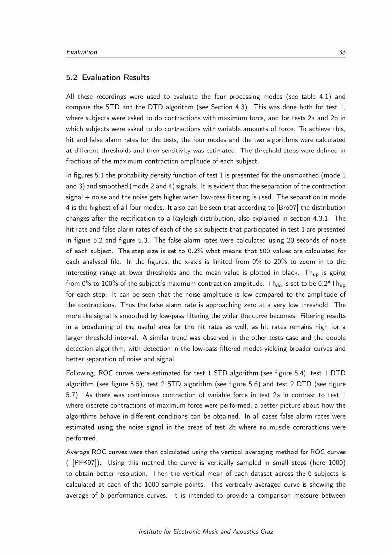
5.2 Evaluation Results

All these recordings were used to evaluate the four processing modes (see table 4.1) andcompare the STD and the DTD algorithm (see Section 4.3). This was done both for test 1,where subjects were asked to do contractions with maximum force, and for tests 2a and 2b inwhich subjects were asked to do contractions with variable amounts of force. To achieve this,hit and false alarm rates for the tests, the four modes and the two algorithms were calculatedat different thresholds and then sensitivity was estimated. The threshold steps were defined infractions of the maximum contraction amplitude of each subject.

In figures 5.1 the probability density function of test 1 is presented for the unsmoothed (mode 1and 3) and smoothed (mode 2 and 4) signals. It is evident that the separation of the contractionsignal + noise and the noise gets higher when low-pass filtering is used. The separation in mode4 is the highest of all four modes. It also can be seen that according to [Bro07] the distributionchanges after the rectification to a Rayleigh distribution, also explained in section 4.3.1. Thehit rate and false alarm rates of each of the six subjects that participated in test 1 are presentedin figure 5.2 and figure 5.3. The false alarm rates were calculated using 20 seconds of noiseof each subject. The step size is set to 0.2% what means that 500 values are calculated foreach analysed file. In the figures, the x-axis is limited from 0% to 20% to zoom in to theinteresting range at lower thresholds and the mean value is plotted in black. Th

up

is goingfrom 0% to 100% of the subject’s maximum contraction amplitude. Th

do

is set to be 0.2*Thup

for each step. It can be seen that the noise amplitude is low compared to the amplitude ofthe contractions. Thus the false alarm rate is approaching zero at a very low threshold. Themore the signal is smoothed by low-pass filtering the wider the curve becomes. Filtering resultsin a broadening of the useful area for the hit rates as well, as hit rates remains high for alarger threshold interval. A similar trend was observed in the other tests case and the doubledetection algorithm, with detection in the low-pass filtered modes yielding broader curves andbetter separation of noise and signal.

Following, ROC curves were estimated for test 1 STD algorithm (see figure 5.4), test 1 DTDalgorithm (see figure 5.5), test 2 STD algorithm (see figure 5.6) and test 2 DTD (see figure5.7). As there was continuous contraction of variable force in test 2a in contrast to test 1where discrete contractions of maximum force were performed, a better picture about how thealgorithms behave in different conditions can be obtained. In all cases false alarm rates wereestimated using the noise signal in the areas of test 2b where no muscle contractions wereperformed.

Average ROC curves were then calculated using the vertical averaging method for ROC curves( [PFK97]). Using this method the curve is vertically sampled in small steps (here 1000)to obtain better resolution. Then the vertical mean of each dataset across the 6 subjects iscalculated at each of the 1000 sample points. This vertically averaged curve is showing theaverage of 6 performance curves. It is intended to provide a comparison measure between


Evaluation 34

0 0.02 0.04 0.06 0.08 0.1 0.12 0.140

0.02

0.04

0.06

0.08

0.1

0.12

0.14

0.16

0.18

Observed Value

PD

F-V

alue

PDF: Noise

Rayleigh

PDF: Signal + Noise

0 0.005 0.01 0.015 0.02 0.025 0.03 0.035 0.040

0.02

0.04

0.06

0.08

0.1

0.12

0.14

0.16

0.18

Observed Value

PD

F-V

alue

Gauss

PDF: Noise

PDF: Signal + Noise

!0.02 0 0.02 0.04 0.06 0.08 0.1 0.12 0.14

0.2

0.4

0.6

0.8

1

1.2

Observed Value

PD

F!V

alu

e

PDF: Signal + Noise

Gauss

mode 1

0 0.002 0.004 0.006 0.008 0.01 0.012 0.014 0.016 0.018 0.020

0.02

0.04

0.06

0.08

0.1

0.12

0.14

0.16

0.18

Observed Value

PD

F!V

alu

e

PDF: Signal + Noise

Rayleigh

mode 2

Gauss

PDF: Noise

PDF: Signal + Noise

PDF: Noise

Rayleigh

PDF: Signal + Noise

mode 3

mode 4

0 0.02 0.04 0.06 0.08 0.1 0.12 0.140

0.02

0.04

0.06

0.08

0.1

0.12

0.14

0.16

0.18

Observed Value

PD

F-V

alu

e

PDF: Noise

Rayleigh

PDF: Signal + Noise

0 0.005 0.01 0.015 0.02 0.025 0.03 0.035 0.040

0.02

0.04

0.06

0.08

0.1

0.12

0.14

0.16

0.18

Observed ValueP

DF-

Val

ue

Gauss

PDF: Noise

PDF: Signal + Noise

Figure 5.1: Histogram of noise and contraction signals (test 1) ofsubject 3 for mode 1, 2, 3 and 4.

the different algorithms. An alternative way would be to calculate an average curve based onaveraging the hit and false alarm rates across the six users for the same thresholds. The firstmethod was preferred here as the goal is to compare the algorithms and not to provide thresholdestimators. That is why this algorithm is chosen in this work. As in this method the curve isaveraged only in the y-direction it is the most optimistic way of averaging. Threshold averagingwould also provide an informative threshold comparison.

By observing figure 5.8 we can see that the low-pass filtered algorithms perform better than theother two in both tests and both the single and the double detection algorithm. This was clearwhen observing the histograms, but it is also verified when observing the mean ROC curves. Ofthe two low-pass filtered algorithms, mode 4 seems to have a small advantage in comparisonto mode 2, especially when considering test 2 where contractions of variable intensity whereperformed. In addition, a small improvement in detection for the DTD algorithm can be seenwhen comparing the single threshold ROC curves (fig. 5.6) and the double threshold ROCcurves (fig. 5.7). A slightly higher hit rate is obtained for the same range of false alarms.This improvement can be verified also in figure 5.8 where the average curves according to thevertical averaging algorithm are plotted for the four modes, the two algorithms and the twotests used in the evaluation.

Finally, the above results are plotted in sensitivity space. Figure 5.9 shows a linear model of theZ-transformed ROC curves, obtained by linear regression on the vertically averaged curve datafor all modes and tests. These curves have a slope different than one, because the variancein the noise and contraction signals is not equal (see figure 5.1). In [MC04] MacMillan and


Evaluation 35

0 2 4 6 8 10 12 14 16 18 200

0.1

0.2

0.3

0.4

0.5

0.6

0.7

0.8

0.9

1

Threshold

Fals

e A

larm

Rat

e -

len

gth

(no

ise

sig

nal

ove

r T

H)

/ le

ng

th(n

ois

e s

ign

al)

user1user2user3user4user5user6mean

0 2 4 6 8 10 12 14 16 18 200

0.1

0.2

0.3

0.4

0.5

0.6

0.7

0.8

0.9

1

Threshold

Fals

e A

larm

Rat

e -

len

gth

(no

ise

sig

nal

ove

r T

H)

/ le

ng

th(n

ois

e s

ign

al)


0 2 4 6 8 10 12 14 16 18 200

0.1

0.2

0.3

0.4

0.5

0.6

0.7

0.8

0.9

1

Threshold

Fals

e A

larm

Rat

e -

len

gth

(no

ise

sig

nal

ove

r T

H)

/ le

ng

th(n

ois

e s

ign

al)


0 2 4 6 8 10 12 14 16 18 200

0.1

0.2

0.3

0.4

0.5

0.6

0.7

0.8

0.9

1

Threshold

Fals

e A

larm

Rat

e -

len

gth

(no

ise

sig

nal

ove

r T

H)

/ le

ng

th(n

ois

e s

ign

al)


mode 1 mode 2

mode 3 mode 4

Figure 5.2: False alarm rates vs. threshold steps (test 1, singlethreshold): (1) mode 1, (2) mode 2, (3) mode 3, (4) mode 4

mode 1 mode 2

mode 3 mode 4

0 10 20 30 40 50 60 70 80 90 1000

0.1

0.2

0.3

0.4

0.5

0.6

0.7

0.8

0.9

1

Threshold

Hit

Rat

e -

len

gth

(te

st s

ign

al o

ver

TH

) /

len

gth

(te

st s

ign

al)


0 10 20 30 40 50 60 70 80 90 1000

0.1

0.2

0.3

0.4

0.5

0.6

0.7

0.8

0.9

1

Threshold

Hit

Rat

e -

len

gth

(te

st s

ign

al o

ver

TH

) /

len

gth

(te

st s

ign

al)


0 10 20 30 40 50 60 70 80 90 1000

0.1

0.2

0.3

0.4

0.5

0.6

0.7

0.8

0.9

1

Threshold

Hit

Rat

e -

len

gth

(te

st s

ign

al o

ver

TH

) /

len

gth

(te

st s

ign

al)


0 10 20 30 40 50 60 70 80 90 1000

0.1

0.2

0.3

0.4

0.5

0.6

0.7

0.8

0.9

1

Threshold

Hit

Rat

e -

len

gth

(te

st s

ign

al o

ver

TH

) /

len

gth

(te

st s

ign

al)


Figure 5.3: Hit rates vs. threshold steps (test 1, single threshold): (1)mode 1, (2) mode 2, (3) mode 3, (4) mode 4


Evaluation 36

Table 5.1: Values of da2 and d2 for all filter and detection modes fortest 1 and test 2

Da2 D2

Algorithm Mode Da2(test 1) Da2(test 2) D2(test 1) D2(test 2)

Single Threshold

I 1.26 0.73 1.00 0.62

II 4.30 2.44 3.05 1.83

III 2.88 1.92 2.31 1.59

IV 5.07 3.17 3.58 2.35

Double Threshold

I 1.65 0.83 1.30 0.69

II 4.51 2.79 3.26 2.08

III 3.13 2.24 2.42 1.07

IV 5.02 3.43 3.55 2.44

Creelman are presenting different methods for calculating the parameter d’ in the case of ROCcurves with slope different than one. This parameter is useful as it enables the confirmation ofthe observations with respect to the performance of the different algorithms and modes.

Based on a model of sensitivity as described in formula (5.1), one first obtains d2 and d1, whered2 = a, and d1 = �a

b

. The slope of the curve s is then given by s = d2d1 . A single measure of

sensitivity for the curve is then given by Equation 5.2:

z(H) = a+ b ⇤ z(FA) (5.1)

da2 =

r2

1 + s2d2 (5.2)

where z(H) and z(FA) represents the z-transformed of the hit and the false alarm ratio and aand b are the intercept and the slope of the linear model. Alternatively, one can present the d2

value. Results are shown in table 5.1 and are also included in figure 5.9 where the da2 valuesare presented. The d’ estimators confirm the observations made so far, that is that mode 4provides best detection in all cases, followed by mode 2, then mode 3 and last mode 1. DTD isproviding slightly better detection than STD in most of the cases. Detection was overall worsein test 2 compared to test 1.


Evaluation 37

mode 1 mode 2

mode 3 mode 4

0 0.1 0.2 0.3 0.4 0.5 0.6 0.7 0.8 0.9 10

0.1

0.2

0.3

0.4

0.5

0.6

0.7

0.8

0.9

1 ¬ [th: 0]

¬ [th: 0.2004]

¬ [th: 0.4008]

¬ [th: 0.6012]

¬ [th: 0.8016]

¬ [th: 1.002]

¬ [th: 1.2024]

p(False Alarm Rate)

p(H

it R

ate

)

0 0.1 0.2 0.3 0.4 0.5 0.6 0.7 0.8 0.9 10

0.1

0.2

0.3

0.4

0.5

0.6

0.7

0.8

0.9

1

- [th: 0]- [th: 2.6052]- [th: 3.8076]- [th: 4.8096]- [th: 5.8116]

p(False Alarm Rate)

p(H

it R

ate

)

0 0.1 0.2 0.3 0.4 0.5 0.6 0.7 0.8 0.9 10

0.1

0.2

0.3

0.4

0.5

0.6

0.7

0.8

0.9

1

- [th: 0.4008]- [th: 0.6012]- [th: 0.8016]- [th: 1.002]- [th: 1.2024]- [th: 1.4028]- [th: 1.6032]

- [th: 1.8036]- [th: 2.004]

- [th: 2.2044]- [th: 2.4048]

- [th: 2.6052]

p(False Alarm Rate)

p(H

it R

ate

)

0 0.1 0.2 0.3 0.4 0.5 0.6 0.7 0.8 0.9 10

0.1

0.2

0.3

0.4

0.5

0.6

0.7

0.8

0.9

1

- [th: 0]- [th: 0.2004]- [th: 0.4008]- [th: 0.6012]

p(False Alarm Rate)

p(H

it R

ate

)

Figure 5.4: ROC curves for all 4 modes: false alarm rates plottedagainst hit rates (test 1 - STD): (1) mode 1, (2) mode 2,(3) mode 3, (4) mode 4, different lines represent differentsubjects at all 500 threshold steps tested.


Evaluation 38

mode 1 mode 2

mode 3 mode 4

0 0.1 0.2 0.3 0.4 0.5 0.6 0.7 0.8 0.9 10

0.1

0.2

0.3

0.4

0.5

0.6

0.7

0.8

0.9

1

! [th: 0]

! [th: 0.4008]

! [th: 0.8016]

! [th: 1.2024]

p(False Alarm Rate)

p(H

it R

ate

)

0 0.1 0.2 0.3 0.4 0.5 0.6 0.7 0.8 0.9 10

0.1

0.2

0.3

0.4

0.5

0.6

0.7

0.8

0.9

1

- [th: 0]- [th: 0.4008]- [th: 0.6012]- [th: 0.8016]

p(False Alarm Rate)

p(H

it R

ate

)

0 0.1 0.2 0.3 0.4 0.5 0.6 0.7 0.8 0.9 10

0.1

0.2

0.3

0.4

0.5

0.6

0.7

0.8

0.9

1

- [th: 0]- [th: 1.2024]- [th: 1.6032]- [th: 2.4048]

p(False Alarm Rate)

p(H

it R

ate

)

0 0.1 0.2 0.3 0.4 0.5 0.6 0.7 0.8 0.9 10

0.1

0.2

0.3

0.4

0.5

0.6

0.7

0.8

0.9

1

- [th: 0]- [th: 1.6032]- [th: 3.8076]- [th: 5.2104]

p(False Alarm Rate)

p(H

it R

ate

)

Figure 5.5: ROC curves for all 4 modes: false alarm rates plottedagainst hit rates (test 1 - DTD): (1) mode 1, (2) mode 2,(3) mode 3, (4) mode 4, different lines represent differentsubjects at all 500 threshold steps tested.


Evaluation 39

mode 1 mode 2

mode 3 mode 4

0 0.1 0.2 0.3 0.4 0.5 0.6 0.7 0.8 0.9 10

0.1

0.2

0.3

0.4

0.5

0.6

0.7

0.8

0.9

1! [th: 0]

! [th: 0.6012]

! [th: 1.2024]

! [th: 1.8036]

! [th: 2.8056]

p(False Alarm Rate)

p(H

it R

ate)

0 0.1 0.2 0.3 0.4 0.5 0.6 0.7 0.8 0.9 10

0.1

0.2

0.3

0.4

0.5

0.6

0.7

0.8

0.9

1! [th: 0]! [th: 2.8056]! [th: 3.8076]! [th: 5.8116]

! [th: 9.8196]

! [th: 19.8397]

p(False Alarm Rate)

p(H

it R

ate)

0 0.1 0.2 0.3 0.4 0.5 0.6 0.7 0.8 0.9 10

0.1

0.2

0.3

0.4

0.5

0.6

0.7

0.8

0.9

1

[th: 0] [th: 0.6012]

[th: 1.2024]

[th: 1.8036]

[th: 2.8056]

p(False Alarm Rate)

p(H

it R

ate

)

0 0.1 0.2 0.3 0.4 0.5 0.6 0.7 0.8 0.9 10

0.1

0.2

0.3

0.4

0.5

0.6

0.7

0.8

0.9

1

- [th: 0]

- [th: 1.2024]

- [th: 2.8056]

- [th: 3.8076]

- [th: 5.8116]

- [th: 13.8277]

p(False Alarm Rate)

p(H

it R

ate

)

Figure 5.6: ROC curve for all 4 modes - STD, analysed signals: ramprecordings from test 2: (1) mode 1, (2) mode 2, (3) mode 3,(4) mode 4


Evaluation 40

mode 1 mode 2

mode 3 mode 4

0 0.1 0.2 0.3 0.4 0.5 0.6 0.7 0.8 0.9 10

0.1

0.2

0.3

0.4

0.5

0.6

0.7

0.8

0.9

1

! [th: 0]

! [th: 0.4008]

! [th: 0.8016]

! [th: 1.2024]

p(False Alarm Rate)

p(H

it R

ate)

0 0.1 0.2 0.3 0.4 0.5 0.6 0.7 0.8 0.9 10

0.1

0.2

0.3

0.4

0.5

0.6

0.7

0.8

0.9

1! [th: 0]

! [th: 0.6012]

! [th: 1.2024]

! [th: 1.8036]

! [th: 2.8056]

p(False Alarm Rate)

p(H

it R

ate)

0 0.1 0.2 0.3 0.4 0.5 0.6 0.7 0.8 0.9 10

0.1

0.2

0.3

0.4

0.5

0.6

0.7

0.8

0.9

1

! [th: 0]! [th: 0.4008]! [th: 0.8016]! [th: 1.2024]

p(False Alarm Rate)

p(H

it R

ate)

0 0.1 0.2 0.3 0.4 0.5 0.6 0.7 0.8 0.9 10

0.1

0.2

0.3

0.4

0.5

0.6

0.7

0.8

0.9

1

[th: 0] [th: 1.8036] [th: 2.8056] [th: 5.4108]

p(False Alarm Rate)

p(H

it R

ate

)

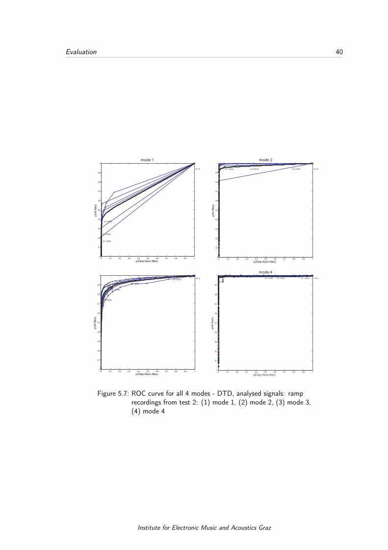
Figure 5.7: ROC curve for all 4 modes - DTD, analysed signals: ramprecordings from test 2: (1) mode 1, (2) mode 2, (3) mode 3,(4) mode 4


Evaluation 41

0 0.2 0.4 0.6 0.8 10

0.1

0.2

0.3

0.4

0.5

0.6

0.7

0.8

0.9

1

ROC ! user study test 1 ! single threshold

p(False Alarm Rate)

p(H

it R

ate

)

mode 1

mode 2

mode 3

mode 4

0 0.2 0.4 0.6 0.8 10

0.1

0.2

0.3

0.4

0.5

0.6

0.7

0.8

0.9

1

ROC ! user study test 2 ! single threshold

p(False Alarm Rate)

p(H

it R

ate

)

mode 1

mode 2

mode 3

mode 4

0 0.2 0.4 0.6 0.8 10

0.1

0.2

0.3

0.4

0.5

0.6

0.7

0.8

0.9

1

ROC ! user study test 1 ! double threshold

p(False Alarm Rate)

p(H

it R

ate

)

mode 1

mode 2

mode 3

mode 4

0 0.2 0.4 0.6 0.8 10

0.1

0.2

0.3

0.4

0.5

0.6

0.7

0.8

0.9

1

ROC ! user study test 2 ! double threshold

p(False Alarm Rate)

p(H

it R

ate

)

mode 1

mode 2

mode 3

mode 4

Figure 5.8: Means of ROC curves of all 4 modes analysing recordings oftest 1: Up: STD Algorithm, Below: DTD Algorithm, Left:test 1 and Right: test 2


Evaluation 42

!3 !2 !1 0 1 2 3!3

!2

!1

0

1

2

3

4

d’ ! user study test 1 ! single threshold

z(False Alarm Rate)

z(H

it R

ate

)

mode 1

mode 2

mode 3

mode 4d!= 1.26

d!= 2.88

d!= 4.30

d!= 5.07

!3 !2 !1 0 1 2 3!3

!2

!1

0

1

2

3

4

d’ ! user study test 2 ! single threshold

z(False Alarm Rate)

z(H

it R

ate

)

mode 1

mode 2

mode 3

mode 4

d!= 0.73

d!= 1.92

d!= 2.44

d!= 3.17

!3 !2 !1 0 1 2 3!3

!2

!1

0

1

2

3

4

d’ ! user study test 1 ! double threshold

z(False Alarm Rate)

z(H

it R

ate

)

mode 1

mode 2

mode 3

mode 4d!= 1.65

d!= 3.13

d!= 4.51

d!= 5.02

!3 !2 !1 0 1 2 3!3

!2

!1

0

1

2

3

4

d’ ! user study test 2 ! double threshold

z(False Alarm Rate)

z(H

it R

ate

)

mode 1

mode 2

mode 3

mode 4d!= 0.83

d!= 2.24

d!= 2.79

d!= 3.43

Figure 5.9: Linear regressed sensitivity d’ curves of all 4 modes analysingrecordings of test 1 and test 2: Up: STD Algorithm, Below:DTD Algorithm, Left: test 1 and Right: test 2. The valuesof d’ show that mode 4 results in the best detection.


43

6 Conclusion

In this work, the background concerning bioelectrical signals from muscle activation was re-searched and presented. Following, a circuit to obtain such signals was designed, created andtested. The circuit can be used in a wearable hardware device for signal acquisition. The re-sulting hardware was used to obtain bioelectrical signals and four different algorithms for signalpre-processing were implemented. Following a user study was performed to obtain discrete andcontinuous muscle activation signals of maximum and of variable intensity. These were usedto compare four signal preprocessing methods and two simple threshold detection algorithms.The comparison was done using detection theory.

The results show that low-pass filtering the envelope of the bioelectric signal provides a goodway for signal preprocessing of muscle activation signals. Obtaining the signal envelope using theHilbert Transform provides a small advantage compared to simple signal rectification. Finally,the DTD algorithm provides a detection advantage compared to the STD algorithm.

Future works could be directed in further developing the signal circuit by implementing analog-digital conversion (ADC) on the circuit board so that the need for an audio interface or anyother ADC device is avoided. As the desired frequency range is small, a lower sampling rateis sufficient. It is further necessary to come up with a way to provide threshold values fordifferent users. This could be achieved using the threshold averaging method. This was notimplemented here, but future work should be directed into investigating how robust thresholdestimators can be calculated and providing a statistical analysis of the results. More complexclassifiers are also a promising future direction so that more complex interaction patterns canbe recognized.

6.1 The live scenario

The proposed system was tested in an live environment where the start and the length ofthe playback of two audio samples were triggered by contractions of the user’s right and leftforearm. The signal processing and DTD algorithm were implemented in the real-time graphicaldataflow programming language PURE DATA (PD). It was shown that under controlled settings(e.g.: no body movements except the movements to activate the forearm muscles) the systemis working reliably and the sample playback can be controlled well. The GUI (graphical userinterface) of this test patch is shown in figure 6.1.

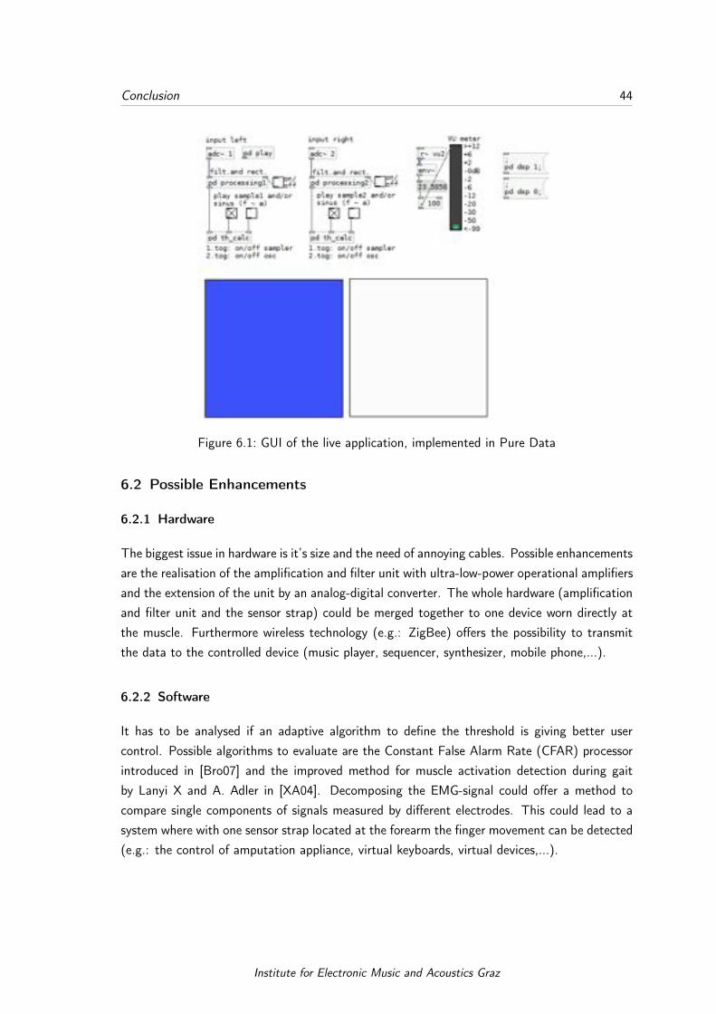
Conclusion 44

Figure 6.1: GUI of the live application, implemented in Pure Data

6.2 Possible Enhancements

6.2.1 Hardware

The biggest issue in hardware is it’s size and the need of annoying cables. Possible enhancementsare the realisation of the amplification and filter unit with ultra-low-power operational amplifiersand the extension of the unit by an analog-digital converter. The whole hardware (amplificationand filter unit and the sensor strap) could be merged together to one device worn directly atthe muscle. Furthermore wireless technology (e.g.: ZigBee) offers the possibility to transmitthe data to the controlled device (music player, sequencer, synthesizer, mobile phone,...).

6.2.2 Software

It has to be analysed if an adaptive algorithm to define the threshold is giving better usercontrol. Possible algorithms to evaluate are the Constant False Alarm Rate (CFAR) processorintroduced in [Bro07] and the improved method for muscle activation detection during gaitby Lanyi X and A. Adler in [XA04]. Decomposing the EMG-signal could offer a method tocompare single components of signals measured by different electrodes. This could lead to asystem where with one sensor strap located at the forearm the finger movement can be detected(e.g.: the control of amputation appliance, virtual keyboards, virtual devices,...).


45

References

[Ach11] Venkatesh Acharya. Improving common-mode rejection using the right-leg driveamplifier, 2011.

[BB10] BURR-BROWN. Datasheet: Precision, low power instrumentation amplifier, 2010.

[BCF+05] Terry D. Blumenthal, A Bruce N. Cuthbert, B Diane L. Filion, Steven Hackley,D Ottmar V. Lipp, and Anton Van Boxtel F. Committee report: Guidelines for hu-man startle eyeblink electromyographic studies. Psychophysiology, 42:1–15, 2005.

[BJ85] de Luca CJ. Basmajian JV. Muscles Alive - The Functions Revealed by Electromyo-graphy. Williams and Wilkins Company, Baltimore, 1985.

[Bro07] Graham Brooker. Detection of Signals in Noise. The University of Sydney, 2007.

[CIA05] Enrico Costanza, Samuel A. Inverso, and Rebecca Allen. Toward subtle intimateinterfaces for mobile devices using an emg controller. In In CHI 05: Proceedingsof the SIGCHI conference on Human factors in computing systems (New), pages481–489. ACM Press, 2005.

[CIAM07] Enrico Costanza, Samuel A. Inverso, Rebecca Allen, and Pattie Maes. Intimateinterfaces in action: assessing the usability and subtlety of emg-based motionlessgestures. In CHI 07, pages 819–828, 2007.

[CJDLR10] Mikhail Kuznetsov Carlo J. De Luca, L. Donald Gilmore and Serge H. Roy. Filter-ing the surface emg signal: Movement artifact and baseline noise contamination.Journal of Biomechanics (05 March 2010), 2010.

[Dis11] Yosemite Community College District. Physiology 101 - chapter 12 - muscle phys-iology, 2011.

[DL97] Carlo J. De Luca. The use of surface electromyography in biomechanics. Journalof Applied Biomechanics, 13(2):135–163, 1997.

[Fri09] A.J. Fridlund. Contour-following integrator for dynamic tracking of electromyo-graphic data. Psychophysiology, 1979/09.

[GD] Atau Tanaka Gilles Dubost. A wireless, network-based biosensor interface for music.

[Hee98] David Heeger. Signal detection theory, 1998.

[JER] M.D. John E. Robinton. Surface EMG vs. Needle EMG.

[Koc07] Volker Maximillian Koch. A factor graph approach to model-based signal separa-tion, 2007.

[Kon05] Peter Konrad. EMG-Fibel: Eine praxisorientierte Einführung in die kinesiologischeElektromyographie. Noraxon INC. USA., 2005.

[Luc02] Carlo J. De Luca. Surface electromyography - detection and recording, 2002.

References 46

[MC04] N.A. Macmillan and C.D. Creelman. Detection Theory: A User’s Guide. Taylor &Francis, 2004.

[NKV+] Ganesh R Naik, Dinesh Kant, Kumar Vijay, Pal Singh, and Marimuthu Palaniswami.Hand gestures for hci using ica of emg.

[PFK97] Foster Provost, Tom Fawcett, and Ron Kohavi. The case against accuracy es-timation for comparing induction algorithms. In In Proceedings of the FifteenthInternational Conference on Machine Learning, pages 445–453. Morgan Kaufmann,1997.

[Pro85] J. Proakis. Probability, random variables and stochastic processes. Acoustics,Speech and Signal Processing, IEEE Transactions on, 33(6):1637–1637, 1985.

[RBK90] Hugh S. Lusted R. Benjamin Knapp. Computer music journal - vol. 14, no. 1 -new performance interfaces 1, 1990.

[RHMY06] M.B.I. Reaz, M.S. Hussain, and F. Mohd-Yasin. Techniques of emg signal analysis- detection, processing, classification and applications, 2006.

[Tan12] David Tanner. Probability and the Normal Distribution. SAGE Publications, Inc.,0 edition, 2012.

[TKA02] Atau Tanaka, R. Benjamin Knapp, and Rue Amyot. Multimodal interaction inmusic using the electromyogram and relative position sensing, 2002.

[TSSB08] Dan Morris T. Scott Saponas, Desney S. Tan and Ravin Balakrishnan. Demon-strating the feasibility of using forearm electromyography for muscle-computer in-terfaces, 2008.

[vB08] Anton van Boxtel. Facial emg as a tool for inferring affective states, 2008.

[Wei06] Martin Weitz. Messung und analyse myoelektrischer signale, 2006.

[Win99] Uwe Windhorst. Modern Techniques in Neuroscience Research. Springer, 1999.

[XA04] Lanyi X and Adler A. An improved method for muscle activation detection duringgait. Canadian Conference of Electrical and Computer Engineering, 2004.

Additional user study recordings 47

A Additional user study recordings

In addition to tests 1, 2a and 2b another test was completed by the subjects. In this test 3stimuli tones of a duration of 1 second are played randomly distributed in the range of C3 toC4. In the pause of 2 seconds between the simuli tones the subject should press the elasticball with the force corresponding to the heard frequency. As it is very difficult for humans torecognise tone pitch this test was not used in the evaluation. An improvement of test 3 wouldbe to use pitch sweeps as stimuli starting at C3 and rising to the desired tone pitch. Thereforeit is more likely that the subject is recognising the correct level.

B Discrete amplifier test setup

The instumentation amplifier was discretely built on a developement board using three TI082operational amplifiers by Texas Instruments. The amplified output V

out

of the instrumentationamplifier (figure 3.4) was screened and stored on a digital oscilloscope. The screen shot of ashort contraction of musculus biceps femoris is shown in figure B.1. Due to the basic circuitdesign and the lack of filtering and protection by enclosure a quite high unwanted 50Hz humoccurred.

Figure B.1: Recorded waveform of a short contraction of musculusbiceps femoris prozessed with the discrete design, analysedwith a digital oscilloscope

Printed circuit board layout 48

C Printed circuit board layout

Figure C.1: Printed circuit board layout of "EMG Machine"

Printed circuit board layout 49

C.1 List of Parts

Table C.1: List of parts required to build ’EMG machine’

Part Description Quantity

EMG machine 2.0 PCB (figure C.1) 1 Pc

Instrumentation Amp. INA 118P 1 Pc

Wideband Feedback Op. Amp OPA2650P 1 Pc

J-FET Input Op. Amp. TL082P 1 Pc

Restisor 220⌦ 2 Pcs

Restisor 1.5 k 1 Pc

Restisor 2.2 k⌦ 1 Pc

Restisor 10 k⌦ 2 Pc



Capacitor 1 µF 2 Pcs

Capacitor 10 nF, 100 pF 1 Pc

Capacitor 100 pF 1 Pc

Diode 1N4004 2 Pcs

PCB Connector 3 Pcs

Metal Housing 1 Pc

Battery 9V 2 Pcs

DC Jack 1 Pc

Audio Plug and Jack mono 1 Pc

Audio Euro Plug and Jack mono 1 Pc

On/Off Switch 1 Pc

Shielded Loudspeaker Cable 8 m

BetterWitts Electrodes 3 Pcs

VELCRO Strap 50 cm

Self Sticking Felt 45 cm2

Snap Fastners 3 Pcs

design and evaluation of an emg-based recording and ... · pdf filetwo ways of detecting the...

Documents