Design and Flight Performance of the Orion

Pre-Launch Navigation System

Renato Zanetti1, Greg Holt2, Robert Gay3, and Christopher D’Souza4

NASA Johnson Space Center, Houston, Texas 77058.

Jastesh Sud5 and Harvey Mamich6

Lockheed Martin Space Systems Company, Denver, CO 80201

Robert Gillis7

Emergent Space Technologies, Denver, CO 80201

The design of the NASA Orion’s prelaunch navigation system is introduced, both

for the first flight test, Exploration Flight Test-1 (EFT-1), and for the first planned

Orion mission, Exploration Mission 1. A detailed trade off of possible design decisions

are discussed and the choices made by Orion are presented. The actual performance of

the navigation system during EFT-1 is presented together with the navigation flight-

software data provided by Orion to the ground controllers in telemetry.

I. Introduction

Arguably one of the greatest successes and glorious applications of the fundamental work of

Rudy Kalman on stochastic estimation [1, 2] is the Apollo onboard navigation filter [3]. The Orion

capsule is NASA’s current flagship human exploration vehicle, is reminiscent of Apollo, and is being

designed to take humans back to the Moon and beyond. The first uncrewed Exploration Mission

1 GN&C Autonomous Flight Systems Engineer, Aeroscience and Flight Mechanics Division, EG6, 2101 NASA Park-way

2 Orion Navigation Co-Lead, Flight Operations Directorate, CM55, 2101 NASA Parkway.3 Orion Vehicle Integration Office Project Lead Engineer, JSC Technical Integration Office, EA4, 2101 NASA Park-way.

4 Navigation Technical Discipline Lead, Aeroscience and Flight Mechanics Division, EG6, 2101 NASA Parkway.5 Software Engineer Staff, M/S B3003, P.O. Box 1796 Orion Navigation Co-Lead, M/S B3003, P.O. Box 1797 GN&C Engineer, M/S B3003, P.O. Box 179

1

(EM-1) is scheduled for 2018, while its first flight test, EFT-1 (Exploration Flight Test-1), was

successfully completed on December 5th, 2014.

Reference [4] describes the navigation design of Orion’s EFT-1 mission and the flight perfor-

mance for the post-lift phase. This paper introduces and presents the complete design of the Orion

pre-launch navigation system; both the EFT-1 design and the changes made for EM-1 and beyond.

This work also documents the performance of the pre-launch navigation system during EFT-1 by

presenting Orion’s telemetry data and discussing the overall navigation results. Reference [5] in-

troduced the preliminary EFT-1 navigation design, while pre-mission simulation performance was

shown in reference. [6]. The UDU factorization as introduced by Bierman is employed in the filter

design [7], and measurements are included as scalars employing the Carlson [8] and Agee-Turner [9]

Rank-One updates. The possibility of considering some of the filter’s states (rather than estimating

all of them [10]) is included in the design [11].

Prior to launch the extended Kalman filter is initialized with the estimated vehicle’s attitude

from gyro compassing (coarse align algorithm) and an inertial position derived from the current

time and the coordinates of the pad. This pre-launch navigation phase is called fine align and the

only measurement active in this mode during EFT-1 was integrated velocity, which is a pseudo-

measurement consisting of a zero change of Earth-referenced position over a 1 second interval. The

GPS receiver measurements are not available during fine align because the vehicle, including the

GPS antennas, is covered by the launch abort fairing. The main purpose of fine align is to better

estimate the attitude in preparation for launch.

The two main contributions of this work are a detailed analysis of ground align measurements

types to feed the Kalman filter and the introduction of a pad position measurement with fully

correlated survey errors between the measurement and the filter’s initial condition. This work also

presents the actual flight telemetry data of Orion EFT-1, hence validating with actual mission data

the design choices.

The fundamental sensor used during Coarse and Fine align is the Inertial Measurement Unit

(IMU), whose EKF model is presented in Section II. The Coarse Align design is presented in III,

while the pre-launch EKF design used for Fine Align is presented in Section IV. The EFT-1 flight

2

performance is presented in Section V followed by concluding remarks.

II. Inertial Measurement Unit

The sections presents the IMU measurement model, which includes both gyros and accelerom-

eters.

A. The Gyro Model

The gyro is modeled in terms of the bias, scale factor, and non-orthogonality. It is taken as

the alignment reference navigation sensor, therefore no gyro misalignment states are included. The

non-orthogonality errors of the IMU case frame are expressed as

Γg =

0 γg3 γg2

γg3 0 γg1

γg2 γg1 0

The gyro scale factor represents the error in conversion from raw sensor outputs (gyro digitizer

pulses) to engineering units. The scale-factor error is modeled as a first-order Markov process in

terms of a diagonal matrix given as

Sg =

sgx 0 0

0 sgy 0

0 0 sgz

Similarly, the gyro bias error is modeled as a first-order vector Markov processes as

bg =

bgx

bgy

bgz

The gyro angular random walk is represented by νg; the model of the gyro’s angular velocity

measurement ωc is given by

ωc = (I3 + Γg + Sg) (ωc + bg + νg) = (I3 + ∆g) (ωc + bg + νg) (1)

where I3 is a 3× 3 identity matrix, the superscript c indicates that this is a measurement expressed

in case-frame co-ordinates, and ωc is the ‘true’ angular velocity in the case frame. Internally the

3

actual measurement from the gyros is an integrated angular rate that, which, if used directly by

the Kalman filter, would produce a suboptimal estimator [12]. Therefore, a coning compensation

algorithm [13] is used internally by the sensor’s firmware.such as the effective measurement is given

by

∆θc

k = ∆θckck−1

=

∫ tk

tk−1

ωc(τ) +1

2∆θ

c(τ)

ck−1× ωc(τ) dτ ∆θ

ck−1

ck−1= 0 (2)

B. The Accelerometer Model

Similar to the gyros, the accelerometer scale factor represents the error in conversion from raw

sensor outputs (accelerometer digitizer pulses) to engineering units and are modeled as a first-order

Markov process in terms of a diagonal matrix given as

Sa =

sax 0 0

0 say 0

0 0 saz

As mentioned in the previous section, the gyro is taken as the aligned sensor while the accelerom-

eter misalignment relative to the gyro is taken into account. The accelerometer misalignment and

nonorthogonality errors are combined and expressed in terms of six different small angles as:

Ξa =

0 ξaxy ξaxz

ξayx 0 ξayz

ξazx ξazy 0

The bias errors are modeled as a first-order Gauss-Markov processes as

ba =

bax

bay

baz

The accelerometer measurements, ac are modeled as:

ac = (I3 + Sa + Ξa) (ac + ba + νa) (3)

where ac is the ‘true’ non-gravitational acceleration in the case frame. The quantity νa is the

velocity random walk.

4

The actual measurement is accumulated acceleration in the case frame, ∆vc, which is mapped

to the end of its corresponding time interval by the sculling algorithm within the IMU firmware

∆vck = ∆vckck−1=

∫ tk

tk−1

Tckc(t)a

c(t) dt (4)

where ∆vck covers the time interval from tk−1 to tk and c(t) is the instantaneous case frame.

The transformation matrix Tckc(t) takes vector coordinates from the case frame at time t to the

case frame at time tk.

III. Coarse Align Design

The Coarse Align Computer Software Unit (CSU) main purpose is to compute an initial estimate

of the attitude of the Orion vehicle while on the pad to initialize the EKF. The output attitude is

based on a simple filtering of high rate IMU data with the assumption that the vehicle has zero

velocity in the Earth-fixed frame.

Orion IMU sensor internal sampling is done at a very high rate to accommodate high rate

compensations such as coning, sculling, size effect, and accelerometer digitizer asymmetry compen-

sation. The high rate data is used to form compensated 200 Hz delta angles and delta velocities in

the body frame. The 200 Hz data is organized in buffers and passed to the Orion flight computer

at 40 Hz. Low pass second order filters are applied to the IMU measurements to remove noise and

oscillatory motion due to wind (twist and sway).

The expected output of the Coarse Alignment, Tce, is the attitude of the IMU case frame

with respect to the Earth-fixed frame (e, or International Terrestrial Reference Frame, ITRF). An

intermediate calculation is T cned, that represents the transformation matrix of the vehicle attitude

with respect to the North-East-Down (NED) frame.

Tce = Tc

ned ×Tnede

The transformation matrix Tnede is determined from the surveyed coordinates of the pad.

A potential algorithm singularity exists if ∆vcfilt and ∆θcfilt vectors are co-linear. This condition

does not occur unless the alignment is done near the north or south pole, however the software

5

contains a check to ensure the |∆θcfilt × Uc| is of reasonable size prior to computing Ec.

IV. Fine Align Design

As previously mentioned, the goal of fine align is to improve the attitude estimate prior to

launch. The only measurement available is the IMU measurement which is used by an EKF in

conjunction with a pseudomeasurement relating the information that, prior to lift-off, the vehicle is

not moving with respect to the pad.

The EKF software is shared between fine align operations and atmospheric flight operations

(ascent, ascent aborts, and entry); all measurements are incorporated in the navigation solution

at 1Hz, which is the GPS measurement rate used during atmospheric flight. The attitude control

algorithm used during atmospheric flight (ascent aborts and entry) necessitates estimates from the

navigation solution at a higher rate than 1 Hz, thus delta velocity delta attitude accumulator (DV-

DAAccum) Computer Software Unit (CSU) is used as the high-rate IMU accumulator and attitude

propagator complement to EKF CSUs in the 1 Hz rate group. The vehicle attitude is propagated

forward in time through the use of accumulated sensed ∆θ data. The CSU also accumulates ∆v

measurements which are used by the Position and Velocity Fast Propagator (PVPropFast) to com-

pute high rate position and velocity for downstream users. The attitude of DVDAAccum and the

state of PVPropFast are re-synched to the 1 Hz rate group estimate each second.

DVDAAccum receives feedback data from the 1 Hz EKF CSUs and uses it to perform an

update. During the update phase DVDAAccum replaces the estimates of the IMU errors with the

most current values from the EKF, transforms the values of the inertial accumulated delta velocity

into the updated inertial frame, and updates the inertial to Orion body attitude with the information

from the filter.

As mentioned above, the Orion fine alignment algorithm utilizes the same Extended Kalman

Filter architecture and CSU as that used for atmospheric navigation (named ATMEKF). This paper

presents the design of the fine align portion of the algorithm and trade studies that were conducted

between three different type of fine align measurements: Integrated Velocity (IV), Zero Velocity

(ZV), and Pad Position (Pos). All these measurements are pseudomeasurents (no sensor exists that

6

produces them) instead the measurements are derived from the known fact that the vehicle is not

moving with respect to the launch pad. Hence the actual measurement utilized in the filter is the

theoretical value corresponding to absence of motion and the measurement error is given by the

variation from this theoretical value due to twist and sway oscillations of the launch stack. This

motion is forced by wind and is a function of the bending modes of the launch system.

The navigation center of computations is given by the IMU location. During EFT-1, the Orion

EKF used an IV measurement during the fine align phase. For EM1 and beyond, three possible

solutions are considered:

1. The IV measurement returns the change in Earth Centered Earth Fixed (ECEF) position over

a specified amount of time, typically the call rate of the EKF, which for EFT-1 is one second.

The processed measurement is always given by the nominal value of zero. The measurement

noise is given by the change of position of the IMU over one second due to twist and sway of

the stack.

2. The pad position (Pos) measurement returns the planet-fixed position of the IMU. This is also a

“fake” measurement always set to the nominal location. The measurement error is comprised

not only to the twist and sway motion, but also of the survey error of the pad location.

Therefore the measurement error has two distinct contributors, a varying component due to

the stack oscillations (modeled as white) and a repeatable component due to the survey errors

(modeled as a random bias).

3. The zero velocity (ZV) measurement returns the instantaneous planet-fixed velocity of the

IMU. This is also always set to the nominal value of zero. The measurement noise is given by

the true velocity of the IMU due to twist and sway of the stack.

In all three cases the twist and sway motion is treated as white noise rather than colored noise

in order to keep the state space smaller and save computations. Thousands of simulated worst-case

scenario robustness analysis runs were performed sweeping large ranges of twist and sway frequencies

and amplitudes. These runs showed the filter robustness with respect to these inputs.

7

A. Integrated Velocity

Given the current inertial position ri at time t, the prior inertial position ri0, as well as the

transformation matrix between Earth-fixed and inertial (Tei ), the IV measurement is given by

yIV = hIV (x,x0, t) + ηIV = Tei (t) ri −Te

i (t0) ri0 + ηIV = 0 (5)

where hIV (x,x0, t) is the measurement model and ηIV is the measurement noise which exactly

cancels out the motion due to twist and sway. The estimated measurement is given by

yIV = hIV (x, x0, t) = Tei (t) ri −Te

i (t0) ri0 (6)

Notice that this measurement is nonlinear, potentially highly-nonlinear, since in order to calculate

ri0 it is necessary to back-integrate the nonlinear equations of motion that also contain the estimates

of the IMU error parameters. The measurement residual is

εIV = yIV − yIV (7)

As a first order approximation (used to obtain the IV measurement partials or measurement mapping

matrix HIV )

εIV =∂hIV∂x

(x− x) +∂hIV∂x0

(x0 − x0) + ηIV (8)

=∂hIV∂x

x +∂hIV∂x0

Φ(t, t0)x + ηIV (9)

= HIV (x) (x− x) + ηIV (10)

8

where Φ(t, t0) is the state transition matrix. With this in mind, the partial derivative of the IV

measurement is as follows

∂hIV∂r

(x) = Tei (t) −Te

i (t0) Φrr(t, t0) (11)

∂hIV∂v

(x) = −Tei (t0) Φrv(t, t0) (12)

∂hIV∂φ

(x) = −Tei (t0) Φrφ(t, t0) (13)

∂hIV∂ba

(x) = −Tei (t0) Φrba

(t, t0) (14)

∂hIV∂sa

(x) = −Tei (t0) Φrsa(t, t0) (15)

∂hIV∂ξa

(x) = −Tei (t0) Φrξa

(t, t0) (16)

∂hIV∂bg

(x) = −Tei (t0) Φrbg (t, t0) (17)

∂hIV∂sg

(x) = −Tei (t0) Φrsg (t, t0) (18)

∂hIV∂γg

(x) = −Tei (t0) Φrγg

(t, t0) (19)

Because of the back-propagation, this measurement is nonlinear in nature. Due to the oscillatory

motion in the flex modes of the stack this nonlinearity could be potentially severe, although severe

nonlinearities are not expected over one second intervals (nor were they experienced during EFT-1).

B. Pad Position Measurement

The position measurement is expressed as follows:

yPos = hPos(x, t) + ηPos = Tei (t) ri + bpad + ηPos (20)

where bpad is the launch pad location survey error and ηPos is the measurement noise which exactly

cancels out the motion due to twist and sway. The estimated measurement is given by

yPos = hPos(x, t) = Tei (t) ri + bpad (21)

The measurement residual is

εPos = yPos − yPos = HPos(x) x + ηPos (22)

9

With this in mind, the partial derivative of the position measurement is as follows

∂hPos∂r

(x) = Tei (t) (23)

∂hPos∂bpad

(x) = I3×3 (24)

Notice that this is a linear measurement and the measurement noise is given by the displacement

due to sway.

C. Zero Velocity

The zero velocity measurement is expressed as follows:

yZV = hZV (x, t) + ηZV = Tei (t)

(vi − ωiE × ri

)+ ηZV = 0 (25)

where ωiE is the Earth angular velocity vector and ηZV is the measurement noise which exactly

cancels out the motion due to twist and sway. The estimated measurement is given by

yZV = hZV (x, t) = Tei (t)

(vi − ωiE × ri

)(26)

The measurement residual is

εZV = yZV − yZV = HZV (x) x + ηZV (27)

With this in mind, the partial derivative of the zero velocity measurement is as follows

∂hZV∂r

(x) = Tei (t) [ωiE×] (28)

∂hZV∂v

(x) = Tei (t) (29)

Notice that this is a linear measurement and the measurement noise is given by the velocity of the

oscillation due to sway.

D. Fine Align Measurement Trade

During factor-of-safety performed prior to EFT-1, the results showed that the IV measurement

is subject to divergence under some higher-than-expected frequency cases. These cases were deemed

extremely unlikely; furthermore the performance of fine align is monitored from the ground which

has the ability to scrub the launch if the atmospheric conditions create excessive oscillatory motion

10

of the stack. While robustness to the amplitude of the oscillations can be achieved via tuning of the

value of the IV measurement noise variance, increasing robustness to very large frequency variations

in the oscillations has no obvious solution. The problem arises from the fact that high frequency of

oscillation make the IV measurement nonlinearities more pronounced.

The IV measurement is inherently a measurement of velocity, or at least average velocity,

since it measures the change in position. Therefore this measurement type provides very little

information on the position of the vehicle. This fact can be seen by the gradual increase of the

position estimation error covariance produced by the filter during fine align. Figure 1 shows linear

covariance analysis results, including the increase in position uncertainty (Fig. 6 in the next section

contains the telemetry covariance from the day of flight and shows a very close match with the

linear covariance analysis results). Very long pad operations can cause the position estimation

error to become excessively large, forcing the ground to send a position re-anchoring command

prior to launch, as routinely done in Space Shuttle missions. Two options are possible for the

re-anchoring: overwriting the state only, hence having a good state estimate but a large, over-

conservative estimation error covariance, or re-initializing the position error covariance as well,

hence losing the correlations between position and all other states.

Fig. 1 Linear covariance analysis showing position, velocity, and attitude 3σ Covariance while

processing IV measurements

11

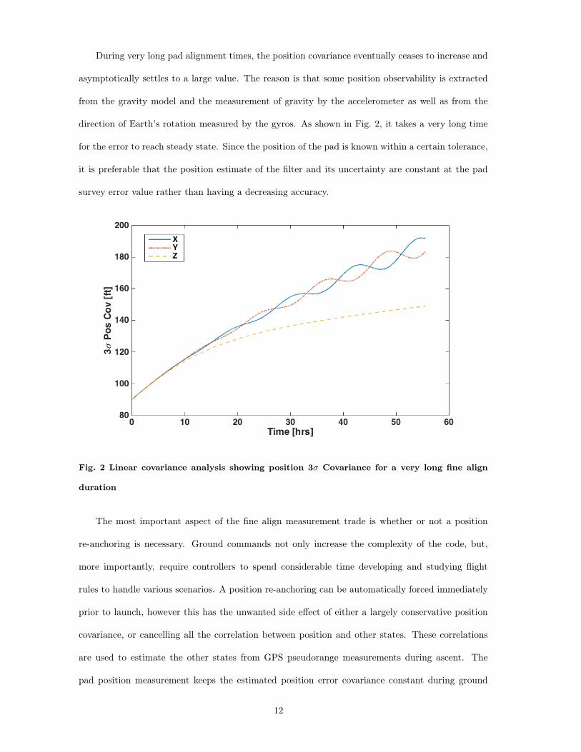
During very long pad alignment times, the position covariance eventually ceases to increase and

asymptotically settles to a large value. The reason is that some position observability is extracted

from the gravity model and the measurement of gravity by the accelerometer as well as from the

direction of Earth’s rotation measured by the gyros. As shown in Fig. 2, it takes a very long time

for the error to reach steady state. Since the position of the pad is known within a certain tolerance,

it is preferable that the position estimate of the filter and its uncertainty are constant at the pad

survey error value rather than having a decreasing accuracy.

Fig. 2 Linear covariance analysis showing position 3σ Covariance for a very long fine align

duration

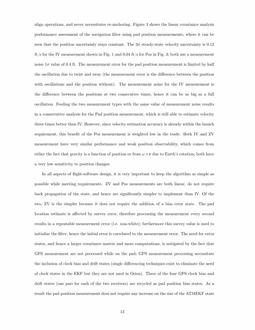
The most important aspect of the fine align measurement trade is whether or not a position

re-anchoring is necessary. Ground commands not only increase the complexity of the code, but,

more importantly, require controllers to spend considerable time developing and studying flight

rules to handle various scenarios. A position re-anchoring can be automatically forced immediately

prior to launch, however this has the unwanted side effect of either a largely conservative position

covariance, or cancelling all the correlation between position and other states. These correlations

are used to estimate the other states from GPS pseudorange measurements during ascent. The

pad position measurement keeps the estimated position error covariance constant during ground

12

align operations, and never necessitates re-anchoring. Figure 3 shows the linear covariance analysis

performance assessment of the navigation filter using pad position measurements, where it can be

seen that the position uncertainty stays constant. The 3σ steady-state velocity uncertainty is 0.12

ft/s for the IV measurement shown in Fig. 1 and 0.04 ft/s for Pos in Fig. 3; both use a measurement

noise 1σ value of 0.4 ft. The measurement error for the pad position measurement is limited by half

the oscillation due to twist and sway (the measurement error is the difference between the position

with oscillations and the position without). The measurement noise for the IV measurement is

the difference between the positions at two consecutive times, hence it can be as big as a full

oscillation. Feeding the two measurement types with the same value of measurement noise results

in a conservative analysis for the Pad position measurement, which is still able to estimate velocity

three times better than IV. However, since velocity estimation accuracy is already within the launch

requirement, this benefit of the Pos measurement is weighted low in the trade. Both IV and ZV

measurement have very similar performance and weak position observability, which comes from

either the fact that gravity is a function of position or from ω×r due to Earth’s rotation; both have

a very low sensitivity to position changes.

In all aspects of flight-software design, it is very important to keep the algorithm as simple as

possible while meeting requirements. ZV and Pos measurements are both linear, do not require

back propagation of the state, and hence are significantly simpler to implement than IV. Of the

two, ZV is the simpler because it does not require the addition of a bias error state. The pad

location estimate is affected by survey error, therefore processing the measurement every second

results in a repeatable measurement error (i.e. non-white); furthermore this survey value is used to

initialize the filter, hence the initial error is correlated to the measurement error. The need for extra

states, and hence a larger covariance matrix and more computations, is mitigated by the fact that

GPS measurement are not processed while on the pad; GPS measurement processing necessitate

the inclusion of clock bias and drift states (single differencing techniques exist to eliminate the need

of clock states in the EKF but they are not used in Orion). Three of the four GPS clock bias and

drift states (one pari for each of the two receivers) are recycled as pad position bias states. As a

result the pad position measurement does not require any increase on the size of the ATMEKF state

13

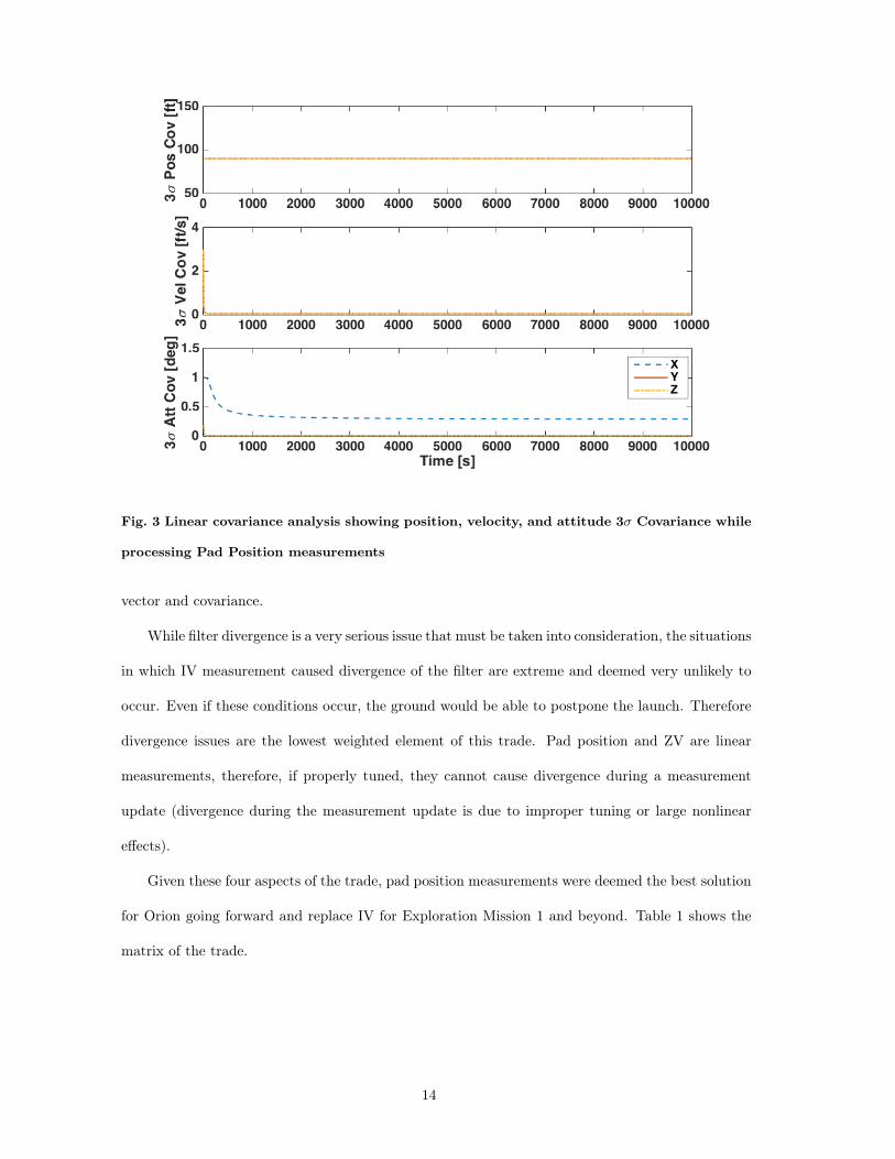
Fig. 3 Linear covariance analysis showing position, velocity, and attitude 3σ Covariance while

processing Pad Position measurements

vector and covariance.

While filter divergence is a very serious issue that must be taken into consideration, the situations

in which IV measurement caused divergence of the filter are extreme and deemed very unlikely to

occur. Even if these conditions occur, the ground would be able to postpone the launch. Therefore

divergence issues are the lowest weighted element of this trade. Pad position and ZV are linear

measurements, therefore, if properly tuned, they cannot cause divergence during a measurement

update (divergence during the measurement update is due to improper tuning or large nonlinear

effects).

Given these four aspects of the trade, pad position measurements were deemed the best solution

for Orion going forward and replace IV for Exploration Mission 1 and beyond. Table 1 shows the

matrix of the trade.

14

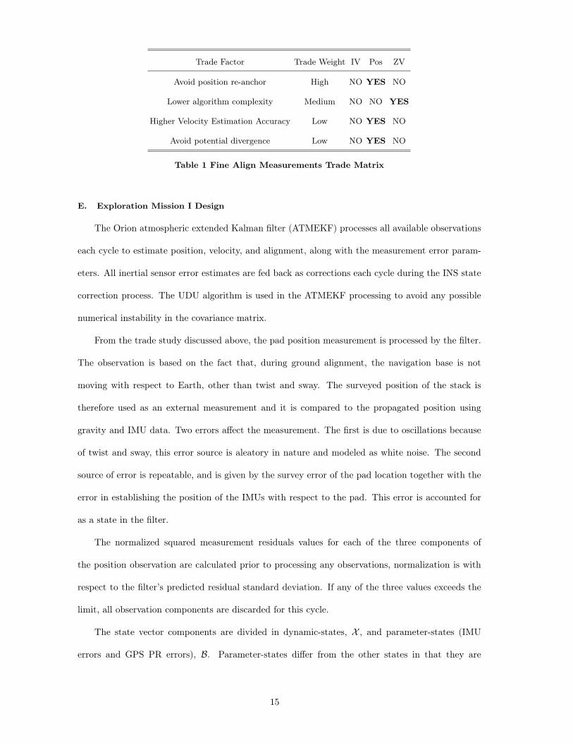
Trade Factor Trade Weight IV Pos ZV

Avoid position re-anchor High NO YES NO

Lower algorithm complexity Medium NO NO YES

Higher Velocity Estimation Accuracy Low NO YES NO

Avoid potential divergence Low NO YES NO

Table 1 Fine Align Measurements Trade Matrix

E. Exploration Mission I Design

The Orion atmospheric extended Kalman filter (ATMEKF) processes all available observations

each cycle to estimate position, velocity, and alignment, along with the measurement error param-

eters. All inertial sensor error estimates are fed back as corrections each cycle during the INS state

correction process. The UDU algorithm is used in the ATMEKF processing to avoid any possible

numerical instability in the covariance matrix.

From the trade study discussed above, the pad position measurement is processed by the filter.

The observation is based on the fact that, during ground alignment, the navigation base is not

moving with respect to Earth, other than twist and sway. The surveyed position of the stack is

therefore used as an external measurement and it is compared to the propagated position using

gravity and IMU data. Two errors affect the measurement. The first is due to oscillations because

of twist and sway, this error source is aleatory in nature and modeled as white noise. The second

source of error is repeatable, and is given by the survey error of the pad location together with the

error in establishing the position of the IMUs with respect to the pad. This error is accounted for

as a state in the filter.

The normalized squared measurement residuals values for each of the three components of

the position observation are calculated prior to processing any observations, normalization is with

respect to the filter’s predicted residual standard deviation. If any of the three values exceeds the

limit, all observation components are discarded for this cycle.

The state vector components are divided in dynamic-states, X , and parameter-states (IMU

errors and GPS PR errors), B. Parameter-states differ from the other states in that they are

15

modeled as first order Markov processes, therefore their time evolution is known analytically and

does not necessitate numerical integration. In addition, their state transition matrix is also known

analytically and it is very sparse, making their covariance matrix propagation extremely numerically

efficient.

X =

[X T BT

]T(30)

The attitude is included as a state in the filter in order to properly model the coupling inherent in

a strap-down IMU. As stated earlier the parameter-states are modeled as first-order Gauss-Markov

processes and use a much more efficient computational algorithm for the update of the covariance

matrix. Tables 2 and 3 list the states and parameters within the Atmospheric EKF. Through

sensitivity analysis, it was determined that accelerometer misalignment and non-orthogonality states

are not a significant contributor to the overall uncertainty and therefore are not included in the filter

state space.

State Number of Description

elements

Position 3 Position vector in inertial coordinates

Velocity 3 Velocity vector in inertial coordinate

Attitude 3 Multiplicative attitude deviation state

Clock Bias and Drift 4 One pair per receiver, three of these states are used as

pad position bias states during fine align

Table 2 Atmospheric Navigation States

Position, velocity, and attitude states and their covariance are initialized as appropriate directly

from data provided to the CSU. During Pad initialization scenarios, states 10 to 12 are initialized

as pad bias states. The pad position measurement is expressed in Earth-fixed coordinates and is

modeled as

ypad = re + bepad + ηpad

where re is the ECEF position vector, bepad is the survey error of the pad position, and ηpad is the

non-repeatable error of the measurement. The filter is initialized with the pad surveyed position

16

Parameter Number of

elements

gyro bias 3

gyro scale factor 3

gyro non-orthogonality 3

accel bias 3

accel scale factor 3

pseudorange bias 12

Table 3 Atmospheric Navigation Parameters

coordinated in the inertial frame, that is, the initial position estimate is given by

r(t0) = Tie(t0) ypad

where Tie is the DCM transforming inertial coordinates into Earth-fixed coordinates, therefore the

initial position estimation error er(t0) is given by

er(t0) = r(t0)− r(t0) = Tie(t0)re −Ti

e(t0)(re + bepad + ηpad) (31)

= −Tie(t0)bepad −Ti

e(t0)ηpad = −Tie(t0)eebpad

−Tie(t0)ηpad (32)

The last equality holds because the initial estimated pad survey error is zero (otherwise the estimate

error would be subtracted from the estimated position resulting in a new estimated position with

zero estimated error). Equation (32) shows the correlation between the initial position and the

survey error state, from it we deduce the values for the following elements of the initial covariance

matrix

P0(bpad, bpad) = Tei (t0) P0(r, r) Ti

e(t0) (33)

P0(X, bpad) = P0(X, r) Tie(t0) (34)

P0(bpad, X) = Tei (t0) P0(r,X) (35)

where P0(bpad, bpad) is the 3× 3 covariance of the pad survey error state, P0(r, r) is the 3× 3 initial

covariance of the position state, P0(X, bpad) is the cross covariance between any state X and the

pad survey error state. Notice that the contribution of the covariance of ηpad is neglected during

17

initialization because is much smaller than the survey error. The resulting 12x12 position, velocity,

attitude, and pad survey error covariance matrix is generally non-diagonal and is converted to its

UDU factorization for the filter to use. Notice that this covariance is singular, however no issues

arise from this fact. If desired, the covariance can be made non-singular by slightly increasing the

position uncertainty by the covariance of ηpad.

V. Pre-Launch EFT-1 Design and Performance

To reduce the computation burden, EFT-1 EKF design did not include GPS PR bias states, refer

to Ref. [4] for more details on the post-liftoff portion of EFT-1 navigation design and performance.

The state-space of EFT-1 navigation filter design is shown in Tables 4 and 5.

State Number of Description

elements

Position 3 Position vector in inertial coordinates

Velocity 3 Velocity vector in inertial coordinate

Attitude 3 Multiplicative attitude deviation state

Clock Bias and Drift 2 Only one GPS receiver used in EFT-1

Table 4 EFT-1 EKF Navigation States

Parameter Number of

elements

gyro bias 3

gyro scale factor 3

gyro non-orthogonality 3

accel high-g bias 3

accel low-g bias 3

accel scale factor 3

accel misalignment and non-orthogonality 6

Table 5 EFT-1 EKF Navigation Parameters

The tuning of the fine align navigation phase for EFT-1 is nearly identical to that of the ascent

18

phase described in Ref. [4], in particular an 8 × 8 gravity field is used, and the process noise is

given by the IMU Angular Random Walk and Velocity Random Walk values. As stated previously,

the IMU states are modeled as first-order Gauss-Markov, a time constant of 4 hours was used (the

total flight duration was 4.5 hours and these errors were expected to remain nearly constant). The

IMU states process noise values are chosen in order to match the steady-state value of the Markov

processes to the vendor’s specification. The integrated velocity error is unique to fine align; it was

determined that an eight inch displacement was the maximum oscillation of the IMU due to twist

and sway motion on the pad, making the peak-to-peak error 16 inches. A one-sigma IV error of 0.4

ft was chosen for EFT-1, which places the worst possible displacement case at a four-sigma value.

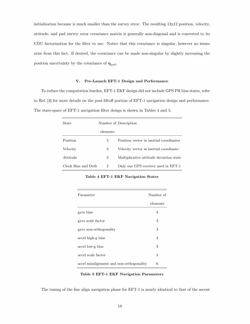
Figure 4 shows the performance of the filter processing this measurement by means of the

measurement residual (actual measurement minus estimated measurement) and their predicted 3σ

standard deviation (dashed lines). It can be seen that the residuals are well within their predicted

standard deviations, all of the measurements are accepted and zero rejections occur. The residuals

are extremely small with respect to their predicted standard deviation, this suggests the filter is

overly conservative. This fact was expected and a design choice shown through simulation to add

robustness to large twist and sway motion of the launch vehicle. During the day of flight little to

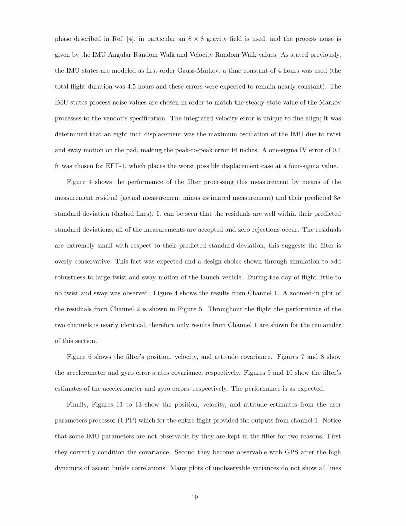
no twist and sway was observed. Figure 4 shows the results from Channel 1. A zoomed-in plot of

the residuals from Channel 2 is shown in Figure 5. Throughout the flight the performance of the

two channels is nearly identical, therefore only results from Channel 1 are shown for the remainder

of this section.

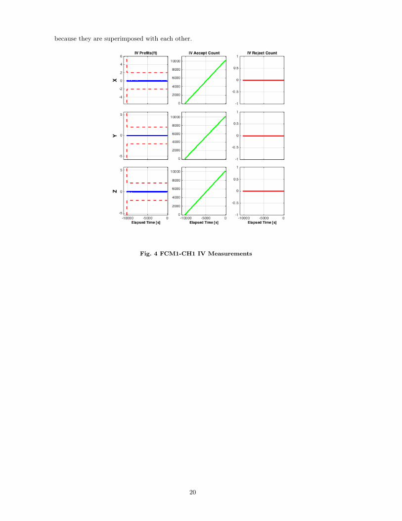
Figure 6 shows the filter’s position, velocity, and attitude covariance. Figures 7 and 8 show

the accelerometer and gyro error states covariance, respectively. Figures 9 and 10 show the filter’s

estimates of the accelerometer and gyro errors, respectively. The performance is as expected.

Finally, Figures 11 to 13 show the position, velocity, and attitude estimates from the user

parameters processor (UPP) which for the entire flight provided the outputs from channel 1. Notice

that some IMU parameters are not observable by they are kept in the filter for two reasons. First

they correctly condition the covariance. Second they become observable with GPS after the high

dynamics of ascent builds correlations. Many plots of unobservable variances do not show all lines

19

because they are superimposed with each other.

Fig. 4 FCM1-CH1 IV Measurements

20

Fig. 5 FCM1-CH2 IV Measurements

Fig. 6 FCM1-CH1 Position, Velocity, and Attitude 3σ Covariance

21

Fig. 7 FCM1-CH1 Accelerometer Bias, Scale Factor, and Misalignment 3σ Covariance

Fig. 8 FCM1-CH1 Gyro Bias, Scale Factor, and Non-Orthogonality 3σ Covariance

22

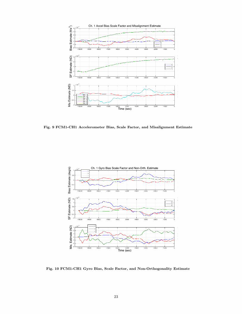
Fig. 9 FCM1-CH1 Accelerometer Bias, Scale Factor, and Misalignment Estimate

Fig. 10 FCM1-CH1 Gyro Bias, Scale Factor, and Non-Orthogonality Estimate

23

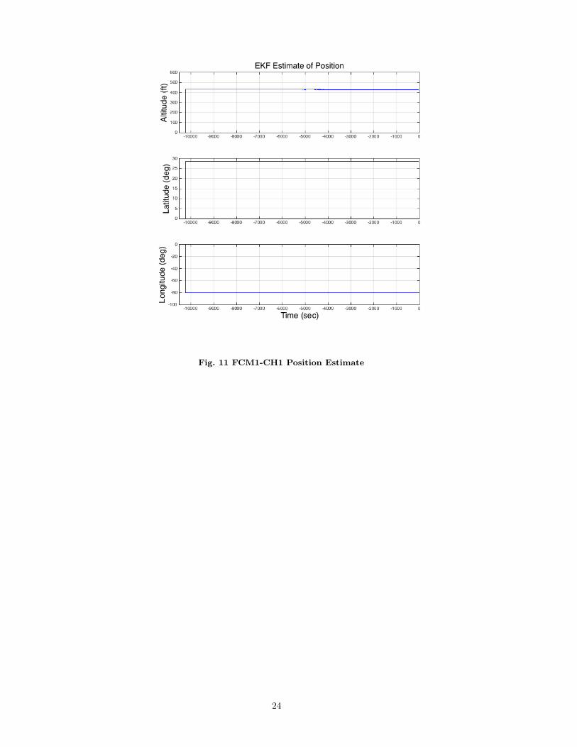
Fig. 11 FCM1-CH1 Position Estimate

24

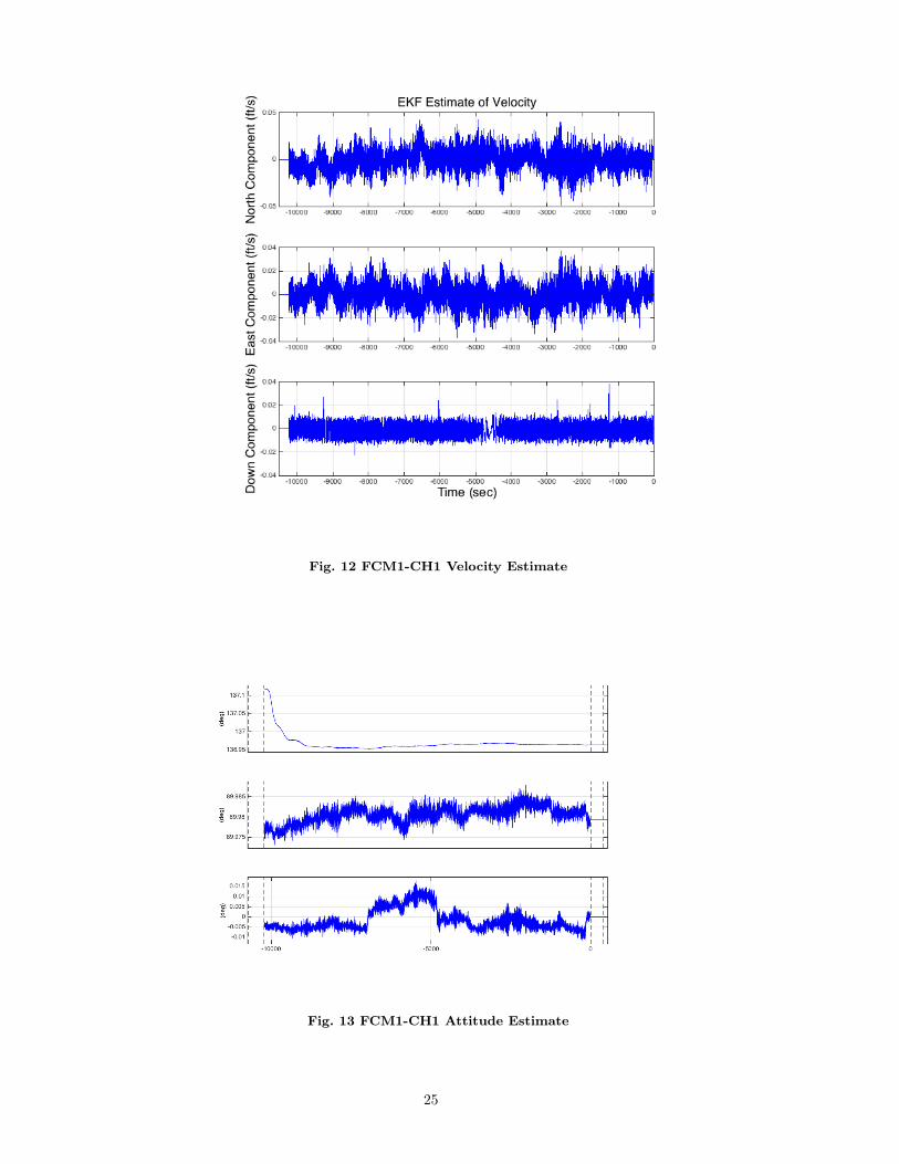
Fig. 12 FCM1-CH1 Velocity Estimate

Fig. 13 FCM1-CH1 Attitude Estimate

25

VI. Conclusions

This paper documents the design of the Orion ground navigation system and presents its per-

formance during Exploration Flight Test 1 (EFT-1). Characteristics of the EFT-1 design are in-

troduced, and data from the flight is shown to validate the design choices. This data illustrates a

flight in which the absolute navigation system performed as expected and produced a good state

to guidance and control. No Integrated Velocity measurement rejections occurred in the filter and

the measurement residuals were very low with respect to their predicted standard deviations. This

fact is due to a combination of conservative tuning of this measurement and perfect weather during

the day of launch. Design trades are also presented to justify the transition from the EFT-1 IV

measurement to the use of Pad Position measurement during future Exploration Mission flights.

The design of the EM1 ground alignment phase is presented in detail.

Aknowledgements

The authors are very thankful to Mike Begley, Daniel Kubitschek, Tim Straube, and Ellis King

for their fundamental role in creating a successful Orion EFT1 pre-launch navigation system.

References

[1] Kalman, R. E., “A New Approach to Linear Filtering and Prediction Problems,” Journal of Basic

Engineering , Vol. 82, No. Series D, March 1960, pp. 35–45, doi:10.1115/1.3662552.

[2] Kalman, R. E. and Bucy, R. S., “New Results in Linear Filtering and Prediction,” Journal of Basic

Engineering , Vol. 83, No. Series D, March 1961, pp. 95–108, doi:10.1115/1.3658902.

[3] Battin, R. H., An Introduction to the Mathematics and Methods of Astrodynamics, AIAA Education

Series, American Institude of Aeronautics and Astronautics, New York, NY, 1987. Pages 751–783.

[4] Zanetti, R., Holt, G. N., Gay, R. S., D’Souza, C., Sud, J., Mamich, H., Bagley, M., King, E., and Clark,

F., “Orion Exploration Flight Test 1 (EFT1) Absolute Navigation Performance,” Journal of Guidance,

Control, and Dynamics, Accepted for publication 2016, doi: 10.2514/1.G002371.

[5] Sud, J., Gay, R., Holt, G., and Zanetti, R., “Orion Exploration Flight Test 1 (EFT1) Absolute Nav-

igation Design,” Proceedings of the AAS Guidance and Control Conference, Vol. 151 of Advances in

the Astronautical Sciences, Breckenridge, CO, January 31–February 5, 2014 2014, pp. 499–509, AAS

14-092.

26

[6] Holt, G., Zanetti, R., and D’Souza, C., “Tuning and Robustness Analysis for the Orion Absolute

Navigation System,” Presented at the 2013 Guidance, Navigation, and Control Conference, Boston,

Massachusetts, August 19–22 2013, AIAA-2013-4876, doi: 10.2514/6.2013-4876.

[7] Bierman, G. J., Factorization Methods for Discrete Sequential Estimation, Vol. 128 of Mathematics in

Sciences and Engineering , Academic Press, 1978. Chapter 5.

[8] Carlson, N. A., “Fast Triangular Factorization of the Square Root Filter,” AIAA Journal , Vol. 11,

No. 9, September 1973, pp. 1259–1265, doi: 10.2514/3.6907.

[9] Agee, W. and Turner, R., “Triangular Decomposition of a Positive Definite Matrix Plus a Symmetric

Dyad with Application to Kalman Filtering,” Tech. Rep. 38, White Sands Missile Range, White Sands,

NM, 1972.

[10] Schmidt, S. F., “Application of State-Space Methods to Navigation Problems,” Advances in Control

Systems, Vol. 3, 1966, pp. 293–340, doi: 10.1016/B978-1-4831-6716-9.50011-4.

[11] Zanetti, R. and D’Souza, C., “Recursive Implementations of the Consider Filter,” Journal of the Astro-

nautical Sciences, Vol. 60, No. 3–4, July–December 2013, pp. 672–685, doi: 10.1007/s40295-015-0068-7.

[12] J.L., and Markley, F.L., “Three-Axis Attitude Estimation Using Rate-Integrating Gyroscopes,” Journal

of Guidance, Control, and Dynamics, Vol. 39, No. 7, 2016, pp. 1513–1526, doi: 10.2514/1.G000336.

[13] Ignagni, M. B., “Efficient Class of Optimized Coning Compensation Algorithms,” Journal of Guidance,

Control, and Dynamics, Vol. 19, No. 2, March–April 1996, pp. 424–429, doi:10.2514/3.21635.

27