design and implementation of a particle image...

Available online at www.sciencedirect.com

Journal

www.elsevier.com/locate/jterra

ScienceDirect

Journal of Terramechanics 50 (2013) 311–326

ofTerramechanics

Design and implementation of a particle image velocimetry methodfor analysis of running gear–soil interaction

Carmine Senatore a,⇑, Markus Wulfmeier a, Ivan Vlahinic b, Jose Andrade b, Karl Iagnemma a

a Laboratory for Manufacturing and Productivity, Massachusetts Institute of Technology, Cambridge, MA 02139, USAb Department of Mechanical and Civil Engineering, California Institute of Technology, Pasadena, CA 91125, USA

Received 24 October 2012; received in revised form 2 July 2013; accepted 29 September 2013Available online 20 October 2013

Abstract

Experimental analysis of running gear–soil interaction traditionally focuses on the measurement of forces and torques developed bythe running gear. This type of measurement provides useful information about running gear performance but it does not allow for expli-cit investigation of soil failure behavior. This paper describes a methodology based on particle image velocimetry for analyzing soilmotion from a sequence of images. A procedure for systematically identifying experimental and processing settings is presented. Soilmotion is analyzed for a rigid wheel traveling on a Mars regolith simulant while operating against a glass wall, thereby imposing plainstrain boundary conditions. An off-the-shelf high speed camera is used to collect images of the soil flow. Experimental results show that itis possible to accurately compute soil deformation characteristics without the need of markers. Measured soil velocity fields are used tocalculate strain fields.� 2013 ISTVS. Published by Elsevier Ltd. All rights reserved.

Keywords: Granular particle image velocimetry; Terrain shearing failure; Wheel dynamics; Off-road vehicle performance

1. Introduction

Particle image velocimetry (PIV) describes an experi-mental method, based on image cross-correlation tech-niques, used for the determination of flow velocity fields.The use of PIV for the calculation of fluid velocities ini-tially emerged in the 1980s [1,2]. Since then, PIV has playedan important role in many fluid mechanics investigations[3,4]. Two of the main advantages of PIV over other meth-ods for the measurement of velocity (e.g. hot-wire-veloci-metry, Pitot tubes, etc.) are that it is non-intrusive, andallows for relatively high resolution measurements overan extended spatial domain.

During fluid-based PIV analysis, the fluid is typicallyseeded with marker particles that refract, absorb, or

0022-4898/$36.00 � 2013 ISTVS. Published by Elsevier Ltd. All rights reserve

http://dx.doi.org/10.1016/j.jterra.2013.09.004

⇑ Corresponding author.E-mail addresses: [email protected] (C. Senatore), [email protected]

(M. Wulfmeier), [email protected] (I. Vlahinic), [email protected](J. Andrade), [email protected] (K. Iagnemma).

scatter light, have a high contrast with the fluid, and donot interrupt the fluid flow. Imaging is performed at highspeed over an area of the flow illuminated by a lightsource, typically a pulsed laser. The resulting light sheetcan be considered as being nearly two-dimensional,because of its low propagation orthogonal to the planeof measured motion [5]. Lasers are typically chosen aslight sources because of their ability to emit high-energy,monochromatic light as thin light sheets. Captured imagesare processed with algorithms that perform frame-to-frame feature tracking and calculation of flow velocityfields.

PIV is also a useful method for measuring soil motion,with the notable constraint that soil is typically observedthrough a glass sheet, limiting the resulting analysis toplain strain scenarios. The natural granular texture of soilsoften generates an intensity pattern that can be traced byPIV, without the use of marker particles. Also, incandes-cent light can generally be used for illumination. Althoughthe term PIV is traditionally associated with fluid

d.


mailto:[email protected]





http://dx.doi.org/016/j.jterra.2013.09.004

http://crossmark.dyndns.org/dialog/?doi=10.1016/j.jterra.2013.09.004&domain=pdf

312 C. Senatore et al. / Journal of Terramechanics 50 (2013) 311–326

mechanics investigation (and the corresponding experimen-tal setup), here we will use the term to refer to the generalconcept of extracting velocity fields from sequences ofimages. This is sometimes referred to as digital imagecorrelation.

Granular PIV has recently been employed in severalapplications, including the analysis of grains in converginghoppers [6], study of flowing granular layers in rotatingtumblers [7], investigation of granular avalanches [8], anal-ysis of soil motion caused by the movement of animals [9],the study of burrowing behavior of razor clams [10], and inthe study of wheel-soil interaction [11,12]. The analysis ofsoil motion beneath a driven wheel via quantitative analy-sis of successive temporal images was first introduced byWong [13]. However, the experimental capabilities of thatstudy did not allow for high-speed image capture, limitingthe accuracy and practical utility of the method.

This paper describes a systematic PIV-based methodol-ogy for analyzing soil motion beneath a running gear (i.e.wheel, track, limb, etc.). A procedure for determining hard-ware and software operational parameters is presented,and various useful techniques for quantitatively analyzingsoil failure are presented. The case of interest in this paperis that of Mars surface exploration by small, lightweightwheeled rovers. Experimental results are thus presentedfor a rigid wheel traveling on a Mars regolith simulant. Ahigh speed camera is used to collect images of the soil flow.Experimental results show that it is possible to compute,with satisfactory accuracy, soil deformation characteristicswithout the need of markers.

The paper is organized as follows: the section entitled“Particle image velocimetry for granular material” presentsa thorough description of experimental setup and a leanintroduction on PIV parameter identification. This sectionalso contains validation and verification experiments, andintroduces a methodology for inferring strain fields fromthe measured velocity fields. The section “Application toanalysis of running gear–soil interaction” shows how PIVcan be used to qualitatively and quantitatively study soilfailure mechanism under running gears. Details on PIVparameter identification and procedures are presented inAppendix A.

2. Particle image velocimetry for granular materials

In this section, a through description of the experimen-tal apparatus is presented and a brief overview of PIV pro-cedures is introduced. Note that in the following, theMatlab-based PIVlab software package is employed [14].Details on how to identify operational parameters forPIVlab can be found in Appendix A.

2.1. Testbed description

The Robotic Mobility Group at MIT has designed andfabricated a multipurpose terramechanics rig based on thestandard design described in [15].

The testbed is pictured in Fig. 1. It is composed of aLexan soil bin surrounded by an aluminum frame to whichall the moving parts, actuators and sensors are attached. Acarriage slides on two low-friction rails to allow longitudi-nal translation while the wheel or track, attached to thecarriage, is able to rotate at a desired angular velocity.The wheel mount is also able to translate in the verticaldirection. This setup allows control of slip and vertical loadby modifying the translational velocity of the carriage,angular velocity of the wheel, and applied load. Horizontalcarriage displacement is controlled through a toothed belt,actuated by a 90 W Maxon DC motor, while the wheel isdirectly driven by another Maxon DC motor. The motorsare controlled thorough two identical Maxon ADS 50/104-Q-DC servo-amplifiers. The carriage horizontal displace-ment is monitored with a Micro Epsilon WPS-1250-MK46draw wire encoder while wheel vertical displacement (i.e.,sinkage) is measured with a Turck A50 draw wire encoder.A 6-axis force/torque ATI Omega 85 transducer ismounted between the wheel mount and the carriage inorder to measure vertical load and traction generated bythe wheel. Finally, a Futek TFF500 flange-to-flange reac-tion torque sensor is used to measure driving torqueapplied to the wheel. Control and measurement signalsare handled by a NI PCIe-6363 card through Labviewsoftware.

The rig is capable of approximately 1 meter of longitu-dinal displacement at a maximum velocity of approxi-mately 0.012 m/s with a maximal wheel angular velocityof approximately 40 deg/s. The bin is 1.2 m long and0.6 m wide while the soil depth is 0.16 m. Considering thewheel sizes and vertical loads under study, these physicaldimensions are sufficient for eliminating boundary effects.Results presented in this paper were obtained with asmooth aluminum wheel with 0.13 m radius and 0.16 mwidth. For PIV tests the wheel angular velocity was fixedat 17 deg/s while the horizontal carriage velocity was mod-ified to achieve the desired slip level. The operational con-ditions described above were chosen because they are closeto those of the Mars Exploration Rover, a successful light-weight robotic vehicle.

2.2. Imager configuration

For the experiments described in this paper, the MojaveMartian Simulant (MMS) was employed as a test medium[16]. MMS is a mixture of finely crushed and sorted gran-ular basalt intended to mimic, at both a chemical andmechanical level, Mars regolith characteristics. The MMSparticle size distribution spans from micron level to mmlevel with 80% of particles above the 10 micron threshold.For the imager configuration described below, resolutionresulted in approximately 5.3 pixels per millimeter.

The accuracy of PIV strongly depends on the quality ofthe captured images. For this study, the Lexan soil bin wasfitted with a 0.0254 m thick tempered glass wall whilethe running gear was operated flush against this surface

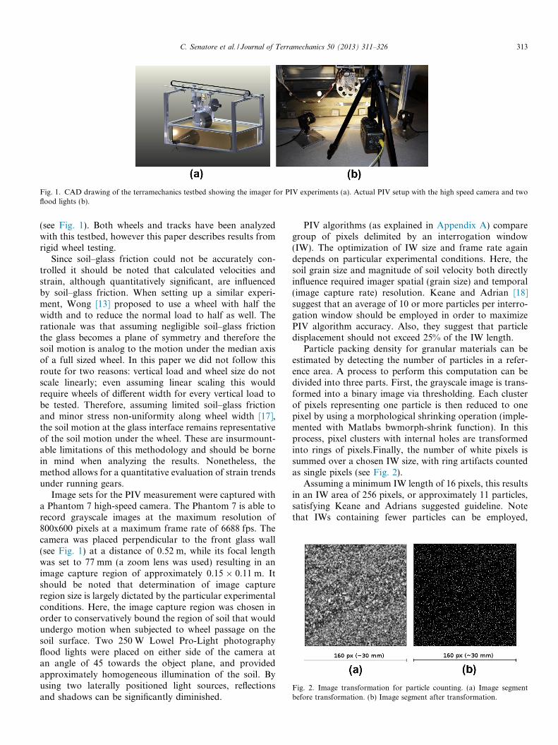
Fig. 1. CAD drawing of the terramechanics testbed showing the imager for PIV experiments (a). Actual PIV setup with the high speed camera and twoflood lights (b).

Fig. 2. Image transformation for particle counting. (a) Image segmentbefore transformation. (b) Image segment after transformation.

C. Senatore et al. / Journal of Terramechanics 50 (2013) 311–326 313

(see Fig. 1). Both wheels and tracks have been analyzedwith this testbed, however this paper describes results fromrigid wheel testing.

Since soil–glass friction could not be accurately con-trolled it should be noted that calculated velocities andstrain, although quantitatively significant, are influencedby soil–glass friction. When setting up a similar experi-ment, Wong [13] proposed to use a wheel with half thewidth and to reduce the normal load to half as well. Therationale was that assuming negligible soil–glass frictionthe glass becomes a plane of symmetry and therefore thesoil motion is analog to the motion under the median axisof a full sized wheel. In this paper we did not follow thisroute for two reasons: vertical load and wheel size do notscale linearly; even assuming linear scaling this wouldrequire wheels of different width for every vertical load tobe tested. Therefore, assuming limited soil–glass frictionand minor stress non-uniformity along wheel width [17],the soil motion at the glass interface remains representativeof the soil motion under the wheel. These are insurmount-able limitations of this methodology and should be bornein mind when analyzing the results. Nonetheless, themethod allows for a quantitative evaluation of strain trendsunder running gears.

Image sets for the PIV measurement were captured witha Phantom 7 high-speed camera. The Phantom 7 is able torecord grayscale images at the maximum resolution of800x600 pixels at a maximum frame rate of 6688 fps. Thecamera was placed perpendicular to the front glass wall(see Fig. 1) at a distance of 0.52 m, while its focal lengthwas set to 77 mm (a zoom lens was used) resulting in animage capture region of approximately 0.15 � 0.11 m. Itshould be noted that determination of image captureregion size is largely dictated by the particular experimentalconditions. Here, the image capture region was chosen inorder to conservatively bound the region of soil that wouldundergo motion when subjected to wheel passage on thesoil surface. Two 250 W Lowel Pro-Light photographyflood lights were placed on either side of the camera atan angle of 45 towards the object plane, and providedapproximately homogeneous illumination of the soil. Byusing two laterally positioned light sources, reflectionsand shadows can be significantly diminished.

PIV algorithms (as explained in Appendix A) comparegroup of pixels delimited by an interrogation window(IW). The optimization of IW size and frame rate againdepends on particular experimental conditions. Here, thesoil grain size and magnitude of soil velocity both directlyinfluence required imager spatial (grain size) and temporal(image capture rate) resolution. Keane and Adrian [18]suggest that an average of 10 or more particles per interro-gation window should be employed in order to maximizePIV algorithm accuracy. Also, they suggest that particledisplacement should not exceed 25% of the IW length.

Particle packing density for granular materials can beestimated by detecting the number of particles in a refer-ence area. A process to perform this computation can bedivided into three parts. First, the grayscale image is trans-formed into a binary image via thresholding. Each clusterof pixels representing one particle is then reduced to onepixel by using a morphological shrinking operation (imple-mented with Matlabs bwmorph-shrink function). In thisprocess, pixel clusters with internal holes are transformedinto rings of pixels.Finally, the number of white pixels issummed over a chosen IW size, with ring artifacts countedas single pixels (see Fig. 2).

Assuming a minimum IW length of 16 pixels, this resultsin an IW area of 256 pixels, or approximately 11 particles,satisfying Keane and Adrians suggested guideline. Notethat IWs containing fewer particles can be employed,

Table 1PIV settings.

Parameter Value Unit

Interrogation window (IW) 16 PixelsFrames per second (fps) 25 fpsResolution 800 � 600 PixelsFrame size 0.15 � 0.11 mCLAHE filter 40 PixelsHigh pass filter Off n/aClipping filter Off n/aIntensity capping filter Off n/aMulti-pass IW sequence 64-32-16 Pixels


however the result is a decrease in accuracy in frame-to-frame feature correlation. Generally, if particle density isunsatisfactorily low, the imager field of view can beadjusted to focus on a smaller spatial soil region.

The experiments analyzed soil motion for conditionswhere the wheel was driven at varying forward velocitiesand slip ratios. The maximum speed of a point on the wheelrim was computed to be 0.038 m/s. Given the imagerparameters described above, this suggests that image cap-ture rate of 25 fps should satisfy the condition that particledisplacement should not exceed 25% of the IW length.Experiments were conducted to verify the effectiveness ofselected conditions, and more broadly, analyze the effectof varying IW sizes and frame rates. The results of thesestudies are reported in [19].

The performance of PIV cross-correlation algorithmsgenerally improves when images are high contrast, featuredense, and have low noise. In practice, images are subjectto non-uniform illumination, imager sensor noise, and lackof natural contrast in the granular material, all of whichcan degrade PIV algorithm performance. Various imagepre-processing methods were investigated to understandtheir effect on algorithm performance. These include com-monly employed algorithms such as contrast limited adap-tive histogram equalization (CLAHE), high pass filtering,and clipping and intensity capping (IC). It was determinedthat optimal performance were achieved with the followingsettings: CLAHE filter with size of 40 pixels, while all otherfilters were disabled.

Motion estimation can be improved through multi-passPIV where the results of each pass are used to improve esti-mation of the IW in the next pass. Several multi-pass com-binations were tested and a three-pass PIV calculationwhich use sequential IW sizes of 64, 32, and 16 pixelswas determined to be a balanced compromise betweenimproved accuracy and calculation times.

The raw velocity field produced by PIV calculations cancontain spurious vectors (outliers). These outliers can becaused by noise, inappropriate interrogation settings, andaccidentally matched patterns. Hence, to improve results,rejection of these outliers and interpolation of missing datapoints can be performed in a post-processing stage throughfiltering. In this study, both global and local filters wereused to reject outliers. Global filters commonly employ asimple thresholding method, with the threshold valueselected by an operator possessing empirical or theoreticaldomain knowledge. If elements of the velocity field exceedthe threshold, this element is removed from the results.Local filters are primarily based on relative differencesbetween surrounding vectors, rather than absolute values.A local filter calculates the mean and standard deviationof the velocity for a selected kernel size around each vector.If the velocity exceeds certain thresholds, the vector isrejected.

The filtering methods described above lead to missingdata in the PIV velocity field. It is frequently desirable tointerpolate missing data points, to yield a complete velocity

field. Interpolation based on surrounding vectors. For thispurpose missing data points were reconstructed throughinterpolation of surrounding velocity vectors.

Final PIV settings adopted in this paper are presented inTable 1.

It should be noted that a masking stage has beenemployed in the results presented in this paper, in orderto eliminate the non-soil image components (i.e. the run-ning gear). Masking can be accomplished through standardimage processing techniques. Masking methods specific torunning gear–soil interaction are described in [19].

2.3. Computation times

This study was conducted on a Windows based 2.4 GHzquad-core machine with 4 GB of RAM. The complete PIVcalculation for an average image set (about 13 s recordingtime) took approximately 60 min. More than two thirdsof this time is spend on the main process, the multi-passcross-correlation. Post-processing and the creation of thevideo file each consume roughly 7% of the total calculationtime. Pre-processing takes only 3% of the total calculationtime.

It should be noted that masking and creation of videofiles are two steps that are not inherently part of the PIVanalysis and do not affect the quality of results. Calculationtimes are summarized in Table 2.

3. Validation and verification

Validation of the PIV algorithm performance was pur-sued on two sets of test data that were physically relevantto the running gear–soil interaction case.

The first test consisted in calculating the velocity fromPIV of a 0.0254 m thick steel plate performing a soil pene-tration test. The ground truth velocity of the plate wasexternally measured by numerically differentiating the out-put of a draw wire encoder which nominally provides aposition measurement. To obtain a plate velocity measurefrom PIV, an average of the velocities was computed overa rectangular region corresponding to the moving plate.

Fig. 3(a) shows a comparison of the plate velocity asdetermined from PIV calculations and the velocitymeasured by the draw wire encoder. The absolute average

Table 2Computation times.

Task Time per image set (270images) [s]

Time per image[s]

(%)

Masking 516 1.91 15Pre-processing 112 0.41 3Cross-correlation 2320 8.59 67Post-processing 257 0.95 7Creation of video

file256 0.95 7

Total time 3461 12.82 100


percent error (for the optimal settings) between these mea-surements was less than 3%. It should be noted that, forthis test case, the PIV algorithm is not performing calcula-tions on the granular soil, but rather the steel plate edge.However, this test remains of interest since the soil in con-tact with the plate necessarily moves at the same velocity.

The second test consisted of calculating the time evolu-tion of motions of discrete features associated with MMSsimulant soil beneath a driven rigid wheel (see Fig. 3(b)).Trajectories s(t) are calculated for a grid of 9 x 6 pointsof interest over the soil area. The time evolution of thepositions of the points of interest was computed by inte-grating the velocities with a fourth order Runge–Kuttamethod.

sðtÞ ¼Z t

0

vðtÞdt ð1Þ

The motion of these tracked particles can be comparedto trajectories of individual soil particles that are largeenough to be manually tracked from frame to frame. Also,the calculation of feature trajectories is useful for illustrat-ing soil flow when subjected to various loading conditions.When compared to non-digital techniques [13], PIV allowsfor systematic quantitative investigation of soil motion. In-depth discussion of observed soil kinematics will be pre-sented in 5.

Fig. 3. (a) Comparison of velocity calculated through PIV and measured witobtained through PIV analysis for a wheel slipping at +30% while advancing tolarge, white particle, is tracked over successive images (images were captured

4. Inferring strain from PIV measurements

The methodology presented thus far allows for precisecalculation of soil motion. The approach yields displace-ment vectors from one captured image to the next at dis-crete pixels inside the image domain. The inferreddisplacements describe a motion of groups of particles.While this provides significant insight in terms of localmaterial response, a more convenient quantity to reportis strain.

Here, the material strain is calculated in a Lagrange ref-erence frame using a large-strain finite element-basedapproach [20–22]. Specifically, we initialize a fixed set ofmaterial points, conveniently defined as the nodal pointsof a finite element mesh at a chosen reference configura-tion. The nodal points are subsequently tracked in time,as they progress through a grid of incremental PIV dis-placements. This approach is favoured over local image-based methods because of the extreme plastic nature of(most) soil materials. In particular, the ability of soil toundergo large plastic deformations arising from micro-structural rearrangement means that PIV must be appliedin an incremental fashion (and not with respect to a singleimage reference).

Below are briefly summarized the non-trivial stepsinvolved in extracting local strains from PIV measurements(as summarized in Fig. 4). All calculations and visualiza-tion were performed in Matlab2012b using an in-houseprogram built for the purpose.

1. A finite element mesh is used to fill the domain occupiedby soil. To this end, we use four-node quadrilateral ele-ments (rather than constant-strain triangular elements)to insure a continuous strain field. The element size ison the order of 8x8 pixels.

2. At each imaged time step, incremental displacements ofall nodes in the finite element mesh are interpolatedfrom PIV results using bi-linear shape functions. The

h a draw wire encoder. (b) Soil trajectories calculated from velocity fieldthe right of the field (right, bottom). A close up of a region of soil where a

at 25 fps).

Fig. 4. Schematic flowchart of strain calculation from PIV data.

Table 3Summary of data collected. Each test was repeated for �30%, �10%, 0%,10%, and 30% slip. Wheel diameter is 0.13 m and wheel width is 0.16 m forall the experiments.

Test type Load [N] Label

Coated wheel standard 70 Std low loadVelocity loose soil 100 Std medium load

130 Std High LoadCoated wheel standard velocity dense soil 130 Dense high loadCoated wheel double velocity loose soil 130 2 V high loadSmooth wheel standard velocity loose soil 130 Loose high load

Table A.4Summary of image canonical transformations adopted to investigate PIVperformance.

Frames Transformation

1–4 Diagonal translation (positive), 1 to 4 pixels5–8 Diagonal translation (negative), 1 to 4 pixels9–12 Horizontal translation, 1 to 4 pixels13–16 Horizontal simple shear, 1 to 4 pixels17–20 Vertical displacement, 1 to 4 pixels21–24 Vertical simple shear, 1 to 4 pixels25–32 Rotation 1 to 8 degrees33–36 Discontinuous shear (upper half moving, 1 to 4 pixels)37–40 Discontinuous shear (both halves moving in opposite directions,

1 to 4 pixels)


process is repeated for all time steps, yielding the cumu-lative displacements at finite element nodes as a functionof time.

3. To determine strain, at each of the 4 Gauss points insidean element, nodal quantities are first converted to adeformation gradient tensor F = dx/dX, that relates avector dx in the deformed state with a vector dX inthe reference state. The deformation gradient tensor iscalculated based on the gradients of the finite elementshape functions. Subsequently, a large strain (Green–Lagrange) tensor is calculated, such that E = FTF � I,where I is a unit tensor. Deviatoric (shear) strain isdefined as �s ¼

ffiffiffiffiffiffiffiffiffiffiffiffi4J 2=3

p, where J2 is the second deviator-

ic strain invariant.4. To visualize the strain field, Gauss point strains are first

transferred back to element nodes and their magnitudeis subsequently plotted over the entire (meshed) domainusing standard element shape functions. Because a con-tinuous mesh describes the soil, the technique makes it

possible to visualize material deformation, and at thesame time, visualize the local strain state in thedeformed finite element mesh.

Representative results of PIV-based strain calculationsare provided in Figs. 8, 9.

5. Application to analysis of running gear–soil interaction

Typically, analysis of running-gear soil interaction relieson the use of a single wheel (or track) test rig that is capableof measuring performance parameters such as applied load,torque, slip ratio, and net thrust. While useful, such testingdoes not provide fundamental insight into soil motion andfailure, nor does it allow for explicit validation of constitu-tive laws relating soil stress to displacement. Granular PIVcan be employed as a complementary testing apparatus to asingle wheel test rig. In this section we present several sim-ple PIV-based analysis and visualization tools for charac-terizing soil response to loading. The tests are conductedunder controlled slip conditions. Slip is defined as:

i ¼ 1� vxr

ð2Þ

where v is the translational velocity of the wheel, x is theangular velocity of the wheel, and r is wheel radius. Bymodifying v and keeping x constant, it is possible to drivethe wheel at desired slip level. In results presented here, thewheel was coated with a layer of MMS bonded to the sur-face with spray glue while tests were performed at 70 N,100 N, and 130 N of vertical load (labeled low, medium,and high load). The wheel was driven at a constant angularvelocity of 17 deg/s, while for higher velocity tests angularvelocity was set to 34 deg/s (these tests were labeled 2 V).Testing conditions are summarized in Table 3. For all thefigures presented in this paper, the wheel is moving fromthe left to the right. (See Table A.4)

5.1. Characterization of soil velocity field

The PIV algorithm generates a velocity vector for eachIW, which results in a closely-spaced array of vectorsdescribing soil motion. An example visualization of sucha result is shown in Fig. 5 (top left). Here, each IW is asso-ciated to a vector, with the vector length corresponding tothe flow velocity and the vector direction aligned with theflow direction. Analysis of such images can provide insightinto the spatial distribution of soil velocity under runninggear, and can vary dramatically for such cases as slip, skid,free-rolling wheels, braked wheels, etc.

Decomposition of this flow field can yield useful insightinto soil shearing (which occurs primarily in the horizontaldirection, see upper right image) and soil compaction phe-nomena (which occurs primarily in the vertical direction,see upper right image). Here, a blue region correspondsto no motion while red indicates a maximum velocity.

Fig. 5. A snapshot of a 30% slip test (Std High Load). Nominal vertical load is 100 N and wheel angular velocity 17 deg/s. From top-left-clockwise:velocity vectors, u-velocity (horizontal component of velocity vector, negative is left), v-velocity (vertical component of velocity vector, negative is up), andvelocity magnitude.

0.5 1 1.5 2 2.5 3 3.5 45

10

15

Time [s]

Soil

Aver

age

Velo

city

[mm

/s]

0 0.5 1 1.5 2 2.5 3 3.5 46

7

8

Torq

ue [N

m]

Soil Average VelocityTorque

Fig. 6. Periodicity of failure zone for a coated wheel under 100 N ofvertical load and +30% slip (Std High Load) is evident when visualizingsoil mean velocity and wheel torque reading. This figure is obtainedcalculating the average velocity of soil motion per frame. The periodicityoccurs at about 2 Hz. Torque reading was not sampled synchronouslywith images therefore a phase shift between the two signals may exist evenif here they have been plotted in phase. Nevertheless, it is remarkable thatsuch close correlation between the two quantities exists, indicating that themeasured wheel telemetry could potentially be used to improve estimationof soil properties below surface and vice versa.


Another phenomenon that was clearly highlighted byPIV analysis is the periodic nature of soil failure. For sliplevel above 10–15%, soil exhibits a periodic loading cycleof alternating compaction and shearing (behavior is pri-marily dilative during the shearing phase), which resultsin discontinuous failure in of the soil mass. This has twodirect consequences: oscillations in drawbar pull/torquereadings, and creation of ripples on the soil surface behindthe wheel. Note that while these effects have been notedpreviously, they have been typically assigned to the effectof grousers [23]. However, these effects are present evenfor smooth wheels, without grousers.Fig. 6 presents soilflow mean velocity for a +30% slip test. Mean velocityoscillation capture the periodic nature of soil failure andare clearly visible also in the torque signal.

Analysis of these images shows that soil flow remainsattached to the wheel rim. Moreover, for low vertical load(such as the one utilized during experiments) it wasobserved that two separate slip failure lines did not evolve,as predicted by classical theory [24,25]. This finding is inter-esting because according to [24], the maximum stressoccurs where the soil flow separates. Also, for slip levelsbelow ±10%, the soil was not observed to develop a signif-icant shearing plane.

5.2. Characterization of soil failure

Traditionally, soil failure under running gear has beenconsidered as an analog of failure under a strip load [26].Following the analogy, two time-independent failure zoneswere predicted under the wheel. A basic approach for

shearing plane identification is to define it based on velocitymagnitude: the deepest point in the soil, where the velocityis above a specified threshold, is identified in each column.A polynomial curve is fitted to these points. Fifth orderpolynomials were used to interpolate the data, sincelower-order representations produced poor results, whilehigher order representations did not improve significantly

Fig. 7. Visualization of shearing planes for a �30% (left) and a +30% (right) slipping wheel (Std High Load). Shearing planes are detected through a linescanning algorithm and the extension of the sheared area depends on the threshold chosen. Because of soil periodic failure, shearing planes are time-varying features. Best viewed in color. (For interpretation of the references to colour in this figure legend, the reader is referred to the web version of thisarticle.)

Fig. 8. (Top) Cumulative deviatoric (shear) strain at different time instants for positive +30% wheel slip (Std High Load). (Bottom) Cumulative deviatoric(shear) strain at different time instants for negative �30% wheel slip. The depth and magnitude of soil disturbance for positive (top) and negative (bottom)wheel slip indicate markedly different soil responses.

Fig. 9. Total deviatoric (shear) strain over 4 time steps, showing localizedfailure region under the wheel. Strain is shown with respect to referenceframe 133, rather than frame 1 as in other the strain plots of Fig. 8. Alocalized shear band is clearly visible. It should be noted that soil underthe wheel is not continuously failing, and therefore failure bands aretypically time-varying features.


the result. According to classical theory, shearing failure isthought to occur along a logarithm spiral, however it wasnot possible to confirm this experimentally.

Identification of a shearing plane depends on the speci-fied velocity threshold. Fig. 7 presents images for �30%(left) and +30% (right) wheel slip, for various velocitythresholds. It is interesting to note that for both slip level,there exists only a single shearing plane. However, it shouldbe noted that soil under the wheel is not continuously fail-ing, and therefore shearing planes are typically time-vary-ing features.

A more systematic way to study the failure zone is tocalculate soil strain as presented in Section 4. Calculationof strain allows for quantitative description of shear bandsand enables more detailed description of soil evolution.Fig. 8 shows a “strain imprint” left behind by a wheel asit travels across the image domain. The depth and

Fig. 10. Horizontal (left), vertical (center), and magnitude (right) of mean flow velocity for slip values ranging from �30% up to +30%. These metricssummarize the results obtained for different soil preparation (dense and loose), different wheel velocity (17 deg/s and 34 deg/s), different vertical load(70 N, 100 N, and 130 N), and different wheel surface finish (smooth and coated with MMS). Note that for dense soil and smooth wheel only one series ofexperiments (at 17 deg/s and 100 N of vertical load) was conducted. Data is obtained by averaging soil motion measured over all the IWs where motionwas detected.


magnitude of soil disturbance for positive (top) and nega-tive (bottom) wheel slip indicate markedly different soilresponses for positive and negative wheel slip conditions.Positive wheel slip produces a shallower soil disturbance,with a clear transition between the disturbed and undis-turbed soil regions.

For 30% positive slip, the largest accumulated strainscan easily surpass 100%, owing to localized failure of thematerial. In contrast, for �30% wheel slip, no localized soilfailures are observed, with soil deformation distributedover a much deeper portion of material, and the largestaccumulated strains consistently below 50%. In both cases,after the wheel has passed, a complex deformation (strain)field is left behind.

In order to visualize shear band formation it is beneficialto isolate a reference frame. This is presented in Fig. 9where strain, for a 30% slipping wheel, is calculated over4 frames. The starting frame (i.e. the reference frame), isconveniently chosen just prior to shear band initiation.Thisallows one to highlight localized shear failure of the gran-ular material during positive wheel slip with the wheel posi-tioned roughly in the center of the image for a better fieldof view. These localized failures occur at periodic intervals,as highlighted in Fig. 6.

5.3. Motion metrics

To grossly summarize results obtained from PIV analy-sis, a series of qualitative metrics was developed. The meanhorizontal velocity, mean vertical velocity, and mean mag-nitude velocity were calculated for each frame, and againover the entire experiment duration. These metrics areintended to give a “snapshot” of collected data and revealthe key trends of soil motion. Results for the experimentsdescribed in Table 3, are presented as function of slip inFig. 10.

For standard velocity tests, the u-velocity rangesbetween �0.2 mm/s and 0.2 mm/s. The u-component

vanishes for 0% slip, where the horizontal motion is causedsolely by compressive motion of the soil, which pushesequally to both directions. Dense soil yields a lower hori-zontal velocity independent of the slip ratio, while experi-ments with the smooth wheel result in reduced horizontalvelocity for high positive slip, due to wheel slip at thewheel-soil interface (and thus reduced soil shearing). Fordoubled rotational velocity, the horizontal component ofthe mean flow is approximately doubled (Fig. 10, left). Thisis intuitively reasonable, because the relative velocitybetween wheel and soil beneath the wheel axle dependsproportionally on the rotational velocity. The vertical com-ponent of the mean flow shows a generally declining trendfrom negative to positive slip ratios. By increasing theweight, the vertical velocity increases, as illustrated in testswith the coated wheel in Fig. 10(center). Dense soil causessignificantly reduced vertical flow. An unexpected trend isshown by all standard tests for 0% slip: The vertical veloc-ity increases compared to �10%.

In these tests, each experiment was performed once andaveraging was performed over all frames of that experi-ment. Experimental variation is likely due to variable soilconditions, despite the fact that an identical soil prepara-tion process was performed for each run. Soil was stirredwith a rod and then leveled. When higher density wasdesired, terrain was compacted with a cylindrical roller.This procedure guaranteed consistent soil preparations atlarge scale.

6. Conclusions

This paper shows how granular particle image velocime-try can enable investigation of running gear–soil interac-tion phenomena. This type of analysis can allow fordevelopment of improved constitutive models for granularmaterials, and for development of reduced order modelsbased on soil displacement predictions. An important con-sideration to bear in mind when examining flow fields like


the one presented in Fig. 5, is that the relationship betweenstress and displacement is typically complex, and one mustavoid the temptation to directly correlate velocity magni-tudes with stress magnitudes.

This paper presented a detailed description of granularparticle image velocimetry methodology for analyzing soilflow under running gears. Although this approach is con-fined to plain strain analysis, it enables detailed quantita-tive and qualitative analysis of soil failure patterns.

A procedure for systematically determining operationalparameters for PIV analysis was presented. The naturaltexture of the granular, dry, material under investigationwas found to be sufficient for PIV analysis eliminatingthe need of markers.

For the experimental setup under investigation it wasfound that only a contrast limited adaptive histogramequalization (CLAHE) pre-processing filter (set to 40 pix-els) was necessary while the best interrogation windowsand multi-pass sequence was found to be 64-32-16 (corre-sponding to IW size, in pixels, for first, second, and thirdpass). Post-processing strategies for outlier detection andsubstitution based on local and global filters were pre-sented as well. The methodology utilized in this paper todetermine the best blend of settings could be in theory uti-lized with any type of soil and imager setup.

It was shown that velocity fields calculated throughgranular PIV can be successfully utilized to infer strainfields. Experimental results show that it is possible to com-pute, with satisfactory accuracy, soil motion characteris-tics. A series of controlled-slip wheel experiments wasperformed and analyzed with the proposed methodologyhighlighting complex soil failure patterns.

Further investigation of small robot-terrain interactionmechanics will focus on extending these experiments to awider range of vertical loads. This will provide a basis forcharacterization of soil plastic internal variable, validationof constitutive laws, and, ultimately, the improvement ofreduced-order models.

Acknowledgements

This study was partially supported by the U.S. ArmyTank Automotive Research, Development and Engineer-ing Center (TARDEC). The Workshop on “xTerrame-chanics – Integrated Simulation of Planetary SurfaceMissions”, sponsored by the Keck Institute for Space Stud-ies at California Institute of Technology (August 2011), hasbeen inspirational to the crafting of this research. Theauthors are grateful to Michele Judd, the managing direc-tor of the Keck Institute for Space Studies, to Dr. JamesW. Bales, the assistant director of the Edgerton Center atMIT, and to A. Sarafraz, J. D’Errico, and W. Thielicke.

Appendix A. Steps for PIV

Soil motion analysis can be broken down into three mainsteps: (1) image pre-processing, (2) image cross-correlation,

and (3) velocity field post-processing. Each step is brieflydescribed and methods for parameter selection arepresented.

A.1. Image pre-processing

Various image pre-processing methods were investigatedto understand their effect on algorithm performance. Theseinclude commonly employed algorithms such as contrastlimited adaptive histogram equalization (CLAHE), highpass filtering, and clipping and intensity capping (IC).

CLAHE differs from basic histogram equalization intwo aspects. First, it computes several histograms, eachfor a separate region of the original image, and thus oper-ates on local parts of the image. Additionally, by limitingthe contrast amplification for a given pixel value, it pre-vents addition of noise to the images. The contrast ofimages used for PIV has a significant influence on the shapeof the correlation plane, which is used for estimation of thevelocities. Hence, pre-processing of the images by optimiz-ing contrast can improve the performance of PIV calcula-tions [27].

High pass filtering reduces low-frequency image inten-sity fluctuations. A high pass filter can remove the back-ground artifacts that are of a lower frequency than thenatural particle texture, and is usually carried out by per-forming basic multiplications on the image in the frequencydomain.

Clipping itself is not a pre-processing filter to increaseimage quality, but rather a method to increase the compu-tation speed through determination of irrelevant areas forthe PIV calculation.

Intensity capping attempts to reject local image intensi-ties which differ too much from their surrounding environ-ment, and could thus degrade the accuracy of the PIV bycausing bias.

To systematically investigate the effect of these pre-pro-cessing methods on PIV algorithm performance, test imagesegments of the Mars regolith simulant with dimensions256 � 256 pixels were captured, and then syntheticallydeformed in canonical directions. Since the particle distri-bution in the soil under investigation is locally not perfectlyhomogeneous, two distinct image segments were capturedin order to adequately represent common grain appearancein the MMS simulant. This resulted in one image popu-lated by relatively large grains (Fig. A.11(a)) and one pop-ulated by relatively small grains (Fig. A.11(b)). Syntheticdeformation of the image was performed as a means ofgenerating a ground truth for cases of linear translation(1–4 pixels in both horizontal, vertical, and diagonal direc-tions), rotation (1–8 degrees in clockwise and counter-clockwise directions), shear (1–4 pixels of relative motionbetween upper and lower image halves), and simple shear(1–4 pixels of motion of the upper edge of image) (seeFigs. A.12, A.13).

A total of 40 transformed images was produced. Sincethe pixel shift for each deformation was controlled, this

Fig. A.11. Examples of soil natural textures: coarse (a) and fine (b).


methodology allowed quantitative evaluation of PIV algo-rithm results. A relative error metric was defined asfollowing:

Fig. A.12. Examples of image canonical transformations used to evaluate PIVused to evaluate PIV accuracy. Transformations included: rigid translationdiscontinuous shear (bottom-right). Details in Table A.4.

Fig. A.13. Velocity field for image transformation, discontinuous shear

� ¼ 1

2N

XN

i

ðui � uiPIV Þ2 þ ðvi � viPIV Þ2 ðA:1Þ

where ui, vi are the true velocity components (based on con-trolled image transformation) at image location i, anduiPIV, viPIV are the velocity components, for the same spa-tial location, estimated through PIV analysis. This isessentially an average mean square error. When thecross-correlation algorithm is not able to calculate a veloc-ity, it returns a NaN value. The error metrics does notaccount for NaN values, however the number of NaNs ismonitored to allow for a comprehensive evaluation of algo-rithm performance.

The forty synthetically deformed images were analyzedunder various combinations of pre-processing settings. Intotal, 96 different combinations of pre-processing parame-ters were studied (see Appendix B for details on pre-pro-cessing parameter combinations).

settings. Nine image transformations for coarse and fine soil textures were(upper-left), simple shear (upper-right), rigid rotation (bottom-left), and

(a) and rotation (b). Largest error occurs at peak velocity gradient.


These tests were conducted using an IW size of 16 � 16pixels. Generally, it was observed that the largest errorsoccurred in shear tests at the simulated failure plane (i.e.the plane of relative motion between the top and bottomhalves of the image), as shown in Fig. A.12. For rotationand simple shear, the largest errors occurred at the imageborders (see Fig. A.13).

Overall, the accuracy of the PIV calculations was foundto be good even without any pre-processing methodapplied. The high level of performance was attributed tothe natural, significant intensity variation present in theMMS simulant, the carefully controlled lighting condi-tions, and the proper selection of imager configuration.

Fig. A.14(a) shows the averaged (over all frames) meansquare error for all the settings. Employing a CLAHE fil-ter with filter sizes of 20 and 40 was found to reduce themean square error. The use of a high pass filter was foundto be uniformly detrimental to PIV calculation accuracywhile a clipping filter was found to be effectively negligi-ble. Intensity capping had a varying effect on accuracy,depending on the other pre-processing settings, howeverits influence was small when other settings are judiciouslychosen. Examining the other dimension of the test space,it can be seen that the mean square error was influencedsignificantly by the different image transformation(Fig. A.14(b)).

Generally, linear translation deformations could beaccurately estimated with a wide range of algorithmparameter settings, whereas rotational transformationsresulted in larger errors. Averaged mean square error forall the frames (Fig. A.14(a)) is usually small becausecross-correlation works particularly well with rigid transla-tion which represent most of the transformations.

As Fig. A.14(b) shows, the highest error levels areobserved during rotation and shear (i.e., when relativelyhigh velocity gradients are present). Those results can becontextualized by noting that the ground truth velocityfor the synthetically deformed images ranged between 0and 8 pixels/frame. Although the average square error isin the order of 0.1 pixels2/frame2, the maximum errorreaches 3 pixels2/frame2 for the most unfavorable (butnot physically unreasonable) conditions.

Although the use of setting # 73 caused relative error toimprove only marginally compared to un-preprocessedimages, it was found that the PIV algorithm producedfewer NaN returns (i.e., areas where the displacementcould not be estimated) with this setting, therefore # 73was adopted. A complete description of the image/pre-pro-cessing parameter combinations and results are presentedin [19].

A.2. Image cross-correlation (PIV)

In PIV, images are divided into small interrogation win-dows (IW) and then analyzed to compute the probable dis-placement between successive images for each IW usingcross-correlation techniques. This results in an equally

spaced field of calculated velocity vectors. The probabledisplacement is determined by using the cross-correlationfunction:

RII�ðx; yÞ ¼XK

i¼�K

XL

j¼�L

Iði; jÞI�ðiþ x; jþ yÞ ðA:2Þ

where I is the intensity of the first image and I0 the intensityof the second image [28]. As noted in Section 2.1, particlepacking density, image resolution, and IW size are inter-connected parameters that must carefully selected to opti-mize performance. Based on experimental investigations,Keane and Adrian [18] defined four empirical rules foroptimal PIV setup. First, the number of particles per IW,NI, should be more than 10:

NI > 10: ðA:3ÞIn-plane particle motion can lead to an inability to com-pute cross-correlation across image pairs, because of thereduction of correlation between particle intensities in bothimages. Hence, the particle displacement XI should not ex-ceed a 25% of the IW length L:

X I <1

4L: ðA:4Þ

Out-of-plane soil motion can cause particles to leave thevisible plane and appear/disappear in different images. Thiseffect again leads to an inability to compute cross-correla-tion across image pairs. For granular PIV, however, it istypically impossible to explicitly control out-of-plane soilmotion. Instead, experiments should be designed in orderto minimize out-of-plane soil flow.

PIV methods compute a velocity vector for an area ofparticles. Since the soil particle velocity in this area is usu-ally not constant, the computed velocity represents anaverage of the velocities of all particles within the area.High gradients in the velocity field will cause the peakin the correlation-plane to broaden. As a guiding rule,the maximum difference of displacement, a, should notexceed the average particle size ds, and also be below5% of the IW length L:

a ¼ jX I ;max � X I ;minja < ds a < 0:05L: ðA:5Þ

It should be noted that while enlarging the IW sizemay allow for better cross-correlation performance,larger IWs result in greater spatial averaging of the flowvelocities. Also, the maximum displacement that can bemeasured depends on the size of the IWs. (The smallerthe chosen IWs are, the shorter the measurabledisplacement.) Ideally, the IW size is chosen to measurethe maximum frame-to-frame displacement, whileminimizing spatial averaging, and yielding good cross-correlation performance. When selection of a static IWsize that yields good performance can be difficult,multi-pass PIV can be employed to achieve improvedperformance.

0 20 40 60 80 1000.05

0.1

0.15

0.2

0.25

0.3

0.35

0.4

Settings

Mea

n Sq

uare

Erro

r [px

/fram

e]2

#73

(a)

0 5 10 15 20 25 30 35 400

0.5

1

1.5

2

2.5

Frames

Mea

n Sq

uare

Erro

r [px

/fram

e]2

(b)Fig. A.14. Pre-processing test space was bi-dimensional: 40 frames � 96 pre-processing settings. Fig. A.14(a) presents the mean square error averaged overall frames. Setting #73 (see Appendix B) was chosen to be the optimal choice because of the good balance of performance (low error and low number ofNaN). Fig. A.14(b) shows the mean square error for pre-processing settings # 73 over all the synthetically deformed images. Performance deteriorates forhigh velocity/velocity gradient corresponding to rigid rotation and shear frames (see Table A.4).

Table A.5Multi-pass settings. Units are in pixels.

Setting # 1st IW 2nd IW 3rd IW 4th IW

1 64 32 16 162 64 32 32 163 64 16 16 –4 64 32 16 –5 32 16 16 –6 32 32 16 –7 64 16 – –8 32 16 – –9 16 – – –


A.2.1. Multi-pass PIV

In multi-pass PIV, multiple PIV calculations are per-formed successively, where the results of each pass are usedto improve estimation of the IW in the next pass.

This can yield improved performance at the cost of addi-tional computation. The simplest approach to multi-passPIV relies on a repetitive determination of a static windowoffset for each IW, which is based on the calculated velocityfrom the prior pass [29].

The multi-pass settings that were evaluated are dis-played in Table A.5. The IW size for each pass was variedbetween 16 pixels and 64 pixels, while the last pass wasalways performed with the previously determined optimumIW size (i.e., 16 pixels). A maximum of four passes wastested. These tests were executed on the previouslydescribed synthetically deformed images and the error isreported as mean square error over all the frames forpre-processing setting # 73.

The mean square error of the velocities computed fromPIV compared to the actual velocities is displayed inFig. A.15. As expected, the use of multi-pass led toimproved performance at the expense of increased process-ing times. Error can be reduced by approximately an orderof magnitude when moving from single-pass PIV (setting #9) to multi-pass. Note that although the minimum errorswere observed for settings # 1, 3, 5 setting # 4 (a three passcalculation) was selected as optimal because it requiredapproximately 30% less computation time while still show-ing a significant improvement with respect to the singlepass setting # 9. To further reduce computation at a costof modestly reduced accuracy, setting # 7 can be employed(a two pass calculation) (see Fig. A.15). Note that the timespresented in Fig. A.15 represent wall clock times for thePIV calculations running on a 2.4 GHz quad-core desktopPC (although the code was not parallelized and Matlabused only one core). A three-pass PIV calculation (setting# 4), which uses sequential IW sizes of 64, 32, and 16 pixelswas considered a balanced choice between accuracy andcomputation times.

A.3. Velocity field post-processing

The raw velocity field produced by PIV calculations cancontain spurious vectors (outliers). These outliers can becaused by noise, inappropriate interrogation settings, andaccidentally matched patterns. Hence, to improve results,rejection of these outliers and interpolation of missing datapoints can be performed in a post-processing stage throughfiltering. Filters for the rejection of outliers can primarilybe divided into two separate classes: global and localmethods.

Global filters commonly employ a simple thresholdingmethod, with the threshold value selected by an operatorpossessing empirical or theoretical domain knowledge. Ifelements of the velocity field exceed the threshold, this ele-ment is removed from the results.

For granular PIV, a global threshold can be defined as amaximum speed for which it is known that no flow vectorwill physically exceed. For the case of running gear–soilinteraction, such a velocity can be determined by comput-ing the maximum velocity, calculated in an inertial frame,of points lying on the running gear itself. For non-dynamictests (i.e. with negligible impact forces), it can be assumedthat no element of the flow field with have a velocitygreater than the maximum running gear velocity.

Local filters are primarily based on relative differencesbetween surrounding vectors, rather than absolute values.

1 2 3 4 5 6 7 8 90

0.02

0.04

0.06

0.08

0.1

0.12

Mea

n Sq

uare

Erro

r [px

/fram

e]2

Multi−Pass Settings1 2 3 4 5 6 7 8 9

0

10

20

30

40

50

60

Tim

e [s

]

Computation TimeMean Square Error

Fig. A.15. Mean square error and computation time for different multi-pass settings. Setting # 9, based on a single pass, produces the worst result.On the right, computation time for different multi-pass settings.

Fig. A.16. Mean square error for different post-processing kernel sizesand threshold settings. These results were obtained for pre-processingsettings # 73 and the synthetically deformed images. High relative errorfor low thresholds is caused by rejection of a high number of vectors (seeFig. A.17, where a wheel experiment is presented). However, even forthreshold that produces low error, it is necessary to verify the number ofrejected vectors in order to produce balanced results.

Fig. A.17. (a) Percentage of rejected vectors for different threshold and kernesize, even at high threshold, a significant portion of vectors are rejected. Partiakernel size 3 � 3 threshold 4; Green, kernel size 5 � 5 threshold 8; Blue, kernel seliminate non-soil regions from the image. (For interpretation of the referencesthis article.)


A local filter calculates the mean and standard deviation ofthe velocity for a selected kernel size around each vector. Ifthe velocity exceeds certain thresholds, the vector is rejected.

Thresholds are defined by the mean velocity plus orminus a number of standard deviations. Such a filter typi-cally operates on the u and v velocity componentsseparately:

umax ¼ umean þ kustd

umin ¼ umean � kustd

vmax ¼ vmean þ kvstd

vmin ¼ vmean � kvstd : ðA:6Þ

The effect of local filter settings on PIV performance wasinvestigated for the synthetically deformed images. Threedifferent kernel sizes (3 � 3, 5 � 5, and 7 � 7 pixels) weretested with thresholds ranging from 1–10 standard devia-tions. The mean square error over these settings is shownin Fig. A.16.

Error decreased for all kernel sizes while the number ofstandard deviations increased the accuracy for lowerthresholds. Increasing the number of standard deviationsalso results in fewer rejected vectors, as displayed inFig. A.17(a), where a wheel experiment is presented.

The large errors observed for low thresholds are a con-sequence of rejecting non-spurious vectors. By increasingthe threshold, a point of minimum error is reached between2–6 standard deviations, depending on the filter size. Errortends to increase for higher thresholds, due to the fact thatsome outliers are retained, which decreases accuracy. Itshould be noted that larger kernel sizes lead to higher com-putational cost, since they require more calculations pervector under consideration.

A.4. Interpolation of missing data points

The filtering methods described above lead to missingdata in the PIV velocity field. It is frequently desirable to

l size obtained for a +30% slipping wheel Fig. (A.17(b)). For 7 � 7 kernell results are overlayed on the right image. Color legend is as follow. Red,ize 7 � 7 threshold 10. Images considered for error analysis were masked toto colour in this figure legend, the reader is referred to the web version of

16 off 15 5 on17 off 15 10 off18 off 15 10 on19 off 30 off off20 off 30 off on21 off 30 5 off22 off 30 5 on23 off 30 10 off24 off 30 10 on25 10 off off off26 10 off off on27 10 off 5 off28 10 off 5 on29 10 off 10 off30 10 off 10 on31 10 5 off off32 10 5 off on33 10 5 5 off34 10 5 5 on35 10 5 10 off36 10 5 10 on37 10 15 off off38 10 15 off on39 10 15 5 off40 10 15 5 on41 10 15 10 off42 10 15 10 on43 10 30 off off44 10 30 off on45 10 30 5 off46 10 30 5 on47 10 30 10 off48 10 30 10 on49 20 off off off50 20 off off on51 20 off 5 off2 20 off 5 on53 20 off 10 off54 20 off 10 on55 20 5 off off56 20 5 off on57 20 5 5 off58 20 5 5 on59 20 5 10 off


interpolate missing data points, to yield a complete velocityfield. Two interpolation approaches are described here:replacement with alternative correlation peaks, and inter-polation based on surrounding vectors.

Spurious correlation results may be caused be a peak inthe correlation plane that is higher than the peak corre-sponding to the real displacement. In this case, the peakcorresponding to the real displacement may still exist inthe correlation plane. Hence, the rejected vector shouldbe replaced by an alternative correlation peak, if this datais available. For this reason, it is common to computelower peaks, and thus if the highest peak does not corre-spond to the true displacement, a lower peak can beemployed. Vectors computed from alternative peaks mustthen be filtered again, to ensure that they are consistentwith respect to the surrounding flow field.

If information about lower correlation peaks is notavailable, missing data in the flow field must be interpo-lated in a different manner. The simplest interpolationmethod is linear interpolation. The value of the currentlymissing vector is simply replaced by information fromneighbouring vectors:

U i ¼1

2ðU i�1 þ Uiþ1Þ: ðA:7Þ

Other interpolation methods can be employed based onnon-linear expressions. Furthermore, it is possible to buildan over-determined system for the local area, and approx-imate the missing vector with a least squares approach [30].It should be noted that while spatial filtering and interpo-lation has been discussed here, similar methods can beemployed for temporal filtering. Due to space constraintsthis discussion is omitted.

Appendix B. Pre-processing settings

Table B.6.

Table B.6Pre-processing settings.

Test CLAHE High pass Clipping IC

1 off off off off2 off off off on3 off off 5 off4 off off 5 on5 off off 10 off6 off off 10 on7 off 5 off off8 off 5 off on9 off 5 5 off10 off 5 5 on11 off 5 10 off12 off 5 10 on13 off 15 off off14 off 15 off on15 off 15 5 off

60 20 5 10 on61 20 15 off off62 20 15 off on63 20 15 5 off64 20 15 5 on65 20 15 10 off66 20 15 10 on67 20 30 off off68 20 30 off on69 20 30 5 off70 20 30 5 on71 20 30 10 off72 20 30 10 on73 40 off off off74 40 off off on75 40 off 5 off76 40 off 5 on77 40 off 10 off78 40 off 10 on79 40 5 off off80 40 5 off on81 40 5 5 off

82 40 5 5 on83 40 5 10 off84 40 5 10 on85 40 15 off off86 40 15 off on87 40 15 5 off88 40 15 5 on89 40 15 10 off90 40 15 10 on91 40 30 off off92 40 30 off on93 40 30 5 off94 40 30 5 on95 40 30 10 off96 40 30 10 on


References

[1] Lauterborn W, Vogel A. Modern optical techniques in fluidmechanics. Annu Rev Fluid Mech 1984;16:223–44.

[2] Dudderar T, Meynart R, Simpkins P. Full-field laser metrology forfluid velocity measurement. Opt Lasers Eng 1988;9(3–4):163–99.doi:10.1016/S0143-8166(98)90002-1. http://www.sciencedirect.com/science/article/pii/S0143816698900021.

[3] Buchhave P. Particle image velocimetrystatus and trends. Exp ThermFluid Sci 1992;5(5):586–604. Special Issue on Experimental Methodsin Thermal and Fluid Science. doi:10.1016/0894-1777(92)90016-X.http://www.sciencedirect.com/science/article/pii/089417779290016X.

[4] Adrian R. Twenty years of particle image velocimetry. Exp Fluids2005;39(2):159–69.

[5] Sveen J, Cowen E. Quantitative imaging techniques and theirapplication to wavy flows. Adv Coastal Ocean Eng 2004;9:1.

[6] Sielamowicz I, Błonski S, Kowalewski T. Digital particle imagevelocimetry (dpiv) technique in measurements of granular materialflows, part 2 of 3-converging hoppers. Chem Eng Sci2006;61(16):5307–17.

[7] Jain N, Ottino J, Lueptow R. An experimental study of the flowinggranular layer in a rotating tumbler. Phys Fluids 2002;14:572.

[8] Pudasaini S, Hsiau S, Wang Y, Hutter K. Velocity measurements indry granular avalanches using particle image velocimetry technique andcomparison with theoretical predictions. Phys Fluids 2005;17:093301.

[9] Barnett C, Bengough A, McKenzie B. Quantitative image analysis ofearthworm-mediated soil displacement. Biol Fertil Soils2009;45(8):821–8.

[10] Winter A. Biologically inspired mechanisms for burrowing inundersea substrates. Ph.D. thesis, Massachusetts Institute of Tech-nology; 2011.

[11] Saengprachatanarug K, Ueno M, Taira E, Okayasu T. Modeling ofsoil displacement and soil strain distribution under a traveling wheel.J Terramech 2012.

[12] Moreland S, Skonieczny K, Wettergreen D, Creager C, Asnani V.Soil motion analysis system for examining wheel-soil shearing. In:17th International conference for the society of terrain-vehiclesystems; 2011.

[13] Wong J. Behaviour of soil beneath rigid wheels. J Agric Eng Res1967;12(4):257–69.

[14] Thielicke W, Stamhuis EJ. PIVlab – time-resolved digital particleimage velocimetry tool for matlab. http://pivlab.blogspot.com/.

[15] Iagnemma K, Shibly H, Dubowsky S. A laboratory single wheeltestbed for studying planetary rover wheel-terrain interaction. MITfield and space robotics laboratory technical report 1; 2005. p. 05–05.

[16] Beegle LW, Peters GH, Mungas GS, Bearman GH, Smith JA,Anderson RC. Mojave martian simulant: a new martian soilsimulant. In: Lunar and planetary institute science conferenceabstracts; 2007.

[17] Senatore C, Wulfmeier M, MacLennan J, Jayakumar P, IagnemmaK. Investigation of stress and failure in granular soils for lightweightrobotic vehicle applications. In: Proceedings of NDIA ground vehiclesystems engineering and technology symposium modeling & simula-tion, testing and validation (MSTV) mini-symposium, Troy, MI;2012.

[18] Keane R, Adrian R. Theory of cross-correlation analysis of pivimages. Appl Sci Res 1992;49(3):191–215.

[19] Wulfmeier M. Development of a particle image velocimetry methodfor analysis of mars rover wheel-terrain interaction phenomena. b.S.thesis, Gottfried Wilhelm Leibniz Universitaet Hannover; April 2012.

[20] Zienkiewicz O, Taylor R. The finite element method: solid mechanics.Finite Element Method Series, vol. 2. Oxford [etc.]: ButterworthHeinemann; 2000. http://books.google.com/books?id=MhgBfMWFV-HUC.

[21] Bazant ZP. Finite strain generalization of small-strain constitutiverelations for any finite strain tensor and additive volumetric-devia-toric split. Int J Solids Struct 1996;33(20):2887–97. http://dx.doi.org/10.1016/0020-7683(96)00002-9. http://www.ingentaconnect.com/con-tent/els/00207683/1996/00000033/00000020/art00002.

[22] Ibrahimbegovic A. Nonlinear solid mechanics: theoretical formula-tions and finite element solution methods. Solid Mech Appl. Springer;2009. http://books.google.com/books?id=z8oI0hCMt40C.

[23] Ding L, Gao H, Deng Z, Nagatani K, Yoshida K. Experimentalstudy and analysis on driving wheels’ performance for planetaryexploration rovers moving in deformable soil. J Terramech2011;48(1):27–45. http://dx.doi.org/10.1016/j.jterra.2010.08.001.http://www.sciencedirect.com/science/article/B6V56-50XRXF0-1/2/ac7e7af600ac1856641535f01c8e1900.

[24] Wong JY. Theory of ground vehicles. 3rd ed. New York: John Wiley& Sons; 2001.

[25] Karafiath LL, Nowatzki EA. Soil mechanics for off-road vehicleengineering. Clausthal, Germany: Trans Tech Publications; 1978.

[26] Bekker MG. Off-the-road locomotion; research and development interramechanics. Ann Arbor: The University of Michigan Press; 1960.

[27] Dellenback P, Macharivilakathu J, Pierce S. Contrast-enhancementtechniques for particle-image velocimetry. Appl Opt2000;39(32):5978–90.

[28] Adrian R, Westerweel J. Particle image velocimetry. CambridgeUniversity Press; 2010. vol. 30.

[29] Westerweel J. Fundamentals of digital particle image velocimetry.Measure Sci Technol 1999;8(12):1379.

[30] Currell G, Dowman A. Essential mathematics and statistics forscience. Wiley; 2009.

http://refhub.elsevier.com/S0022-4898(13)00066-9/h0005































http://pivlab.blogspot.com/



http://dx.doi.org/10.1016/0020-7683(96)00002-9

http://dx.doi.org/10.1016/0020-7683(96)00002-9




















design and implementation of a particle image...

Documents