design and implementation of control system for 6-dof haptic...
TRANSCRIPT

Design and Implementation of Control System for 6-DOF Haptic Device
MOSTAFA SAMADIMALEH
Master of Science ThesisStockholm, Sweden 2011


Design and Implementation of Control System for 6DOF Haptic Device
Mostafa Samadimaleh
Master of Science Thesis MMK 2011:25 MDA 387
KTH Industrial Engineering and Management
Machine Design
SE-100 44 STOCKHOLM


Examensarbete MMK 2011:25 MDA 387
Design och implementering av styrsystem för 6DOF Haptik enhet
Mostafa Samadimaleh
Godkänt
2011-02-03Examinator
Jan WikanderHandledare
Suleman KhanUppdragsgivare
Bengt ErikssonKontaktperson
Bengt Eriksson
Sammanfattning
En haptisk enhet utgör en länk mellan människan och en virtuell miljö simulerad på en dator eller en fjärrstyrd manipulator så kallad tele-manipulering. I båda fallen ska den haptiska enheten ge användaren känslan av vad som händer i verkligheten. Kontakt krafter och moment i den simulerade eller verkliga miljön ska återspeglas till användaren via haptik enheten. Institutionen för Mekatronik på KTH har konstruerat en haptisk enhet kallad Ares vilken kan generera krafter och moment i alla frihetsgrader dvs. sex. Ett av målen inom Ares är att simulera bearbetning av ben vid olika typer av medicinska ingrepp.
Syftet med examensarbetet är att utveckla styrsystemet för den haptiska enheten Ares. För att lyckas med detta så måste enheten modeleras och analyseras för att förstå prestanda och begränsningar. De två övergripande kraven är, i) att användaren inte ska märka av enhetens egendynamik vid kontaktfri rörelse och ii) att servo prestandan för återspegling av kontaktkrafter är snabb och direkt. För att uppfylla detta så konstrueras och jämförs ett antal olika regulatorer med avseende på kraven, för och nackdelar diskuteras i rapporten.
Regulatorerna implementeras på ett prototyputvecklings system från dSPACE där det enkelt går att byta mellan de olika regulatorerna för att snabbt kunna testa och jämföra olika varianter av dessa. Därigenom fås också en verifiering av de modeller som tagits fram under utvecklingsarbetet.

Master of Science Thesis MMK 2011:25 MDA 387
Design and Implementation of Control System for 6DOF Haptic Device
Mostafa Samadimaleh
Approved
2011-02-03Examiner
Jan WikanderSupervisor
Suleman KhanCommissioner
Bengt ErikssonContact person
Bengt Eriksson
Abstract
Haptic devices provide a link between human and a virtual enviroment or remote world. Remote world can be a graphical object in computer or a tele-operation. In both cases, haptic device will give the user feeling of what's happening in reality. Haptic will feed the user back the force and torque of real contact point. A 6-DOF Haptic device namely ARES, has been developed to simulate the bone surgery activities such as drilling, milling or etc .
The aim of this project is to study, partially model, design and implement an appropriate control system for 6-DoF Haptic device. Transparency and force/torque tracking is of high importance objective of the control design which needed to be considered in control design. Hence, in this master thesis, different control approach are studied, implemented and pros and cons of each is discussed.
Later, controllers are implemented on dSpace to investigate performances of the designed controllers. Eventually, as explained in experiment section in details, experimental results confirm the theroy and objective of the controller are achieved.


Acknowledgments
I would like to thank my supervisors at Machine Design department, Bengt Eriksson and Suleman Khan and my examiner, Prof. Jan Wikander for their support during this thesis.
I would also like to take aportunity to thank Felix Hammarstrand for troubleshooting electrical drivers of Haptic Device.


Let us realize that what happens around us is largley outside our control, but that the way we choose to react to it is inside our control.
J.Petty, "Apples of Gold"
To my wife for her patience, undrestanding and support

Contents
1 Introduction 3
1.1 Background . . . . . . . . . . . . . . . . . . . . . . . . . . . . . . . . 3
1.1.1 System Overview . . . . . . . . . . . . . . . . . . . . . . . . . 4
1.1.2 Problem Description . . . . . . . . . . . . . . . . . . . . . . . 6
1.2 Report outline . . . . . . . . . . . . . . . . . . . . . . . . . . . . . . . 7
2 Modeling 8
2.1 Model of ARES . . . . . . . . . . . . . . . . . . . . . . . . . . . . . . 8
2.1.1 Motor Model . . . . . . . . . . . . . . . . . . . . . . . . . . . 10
2.2 Friction Identication . . . . . . . . . . . . . . . . . . . . . . . . . . . 13
2.2.1 Friction Model . . . . . . . . . . . . . . . . . . . . . . . . . . 15
2.2.2 Nonlinear Least Square Method for identication . . . . . . . 16
2.3 Model Validation . . . . . . . . . . . . . . . . . . . . . . . . . . . . . 17
2.4 Conclusion . . . . . . . . . . . . . . . . . . . . . . . . . . . . . . . . . 17
3 Control Design 20
3.1 Introduction . . . . . . . . . . . . . . . . . . . . . . . . . . . . . . . . 20
3.2 Feedback Linearization . . . . . . . . . . . . . . . . . . . . . . . . . 21
3.2.1 Back EMF compensation . . . . . . . . . . . . . . . . . . . . . 22
3.2.2 Friction and Dynamic Compensation . . . . . . . . . . . . . . 23
3.3 Perturbation . . . . . . . . . . . . . . . . . . . . . . . . . . . . . . . . 24
3.3.1 Model Uncertainties . . . . . . . . . . . . . . . . . . . . . . . 25
3.4 PI Torque Control . . . . . . . . . . . . . . . . . . . . . . . . . . . . 26
3.4.1 Stability Analysis . . . . . . . . . . . . . . . . . . . . . . . . . 28
3.5 Optimal H∞ Control . . . . . . . . . . . . . . . . . . . . . . . . . . . 28
3.5.1 Choose Weights . . . . . . . . . . . . . . . . . . . . . . . . . 32
3.5.2 H∞Controller . . . . . . . . . . . . . . . . . . . . . . . . . . . 33
3.5.3 Design of Feed forward Control . . . . . . . . . . . . . . . . . 35
3.5.4 Stability Analysis and Robustness analysis . . . . . . . . . . . 36
3.6 Robust Controller . . . . . . . . . . . . . . . . . . . . . . . . . . . . . 36
3.7 Robust Controller:Second Method . . . . . . . . . . . . . . . . . . . . 42
3.8 Performance Comparison . . . . . . . . . . . . . . . . . . . . . . . . . 43
3.9 Conclusion . . . . . . . . . . . . . . . . . . . . . . . . . . . . . . . . . 44
2
CONTENTS Control of 6-DoF Haptic Device
4 Implementation 454.1 Introduction . . . . . . . . . . . . . . . . . . . . . . . . . . . . . . . . 45
4.1.1 Design Methods . . . . . . . . . . . . . . . . . . . . . . . . . . 464.2 Discretizing Controller . . . . . . . . . . . . . . . . . . . . . . . . . . 46
4.2.1 Choosing Sampling Time Ts . . . . . . . . . . . . . . . . . . . 474.3 Implementation . . . . . . . . . . . . . . . . . . . . . . . . . . . . . . 49
5 Experiments 515.1 Measurements . . . . . . . . . . . . . . . . . . . . . . . . . . . . . . . 51
5.1.1 Position Measurement . . . . . . . . . . . . . . . . . . . . . . 515.1.2 Velocity and Acceleration Estimation . . . . . . . . . . . . . . 515.1.3 Current Measurement and analysis . . . . . . . . . . . . . . . 52
5.2 Controllers . . . . . . . . . . . . . . . . . . . . . . . . . . . . . . . . . 55
6 Future Work and Conclusion 57
7 Appendix 587.1 Controller Implementations . . . . . . . . . . . . . . . . . . . . . . . 58
7.1.1 H∞ . . . . . . . . . . . . . . . . . . . . . . . . . . . . . . . . . 587.1.2 Robust Controller . . . . . . . . . . . . . . . . . . . . . . . . . 587.1.3 Optimal Robust Controller . . . . . . . . . . . . . . . . . . . . 587.1.4 Discritized COntroller . . . . . . . . . . . . . . . . . . . . . . 59
3
Chapter 1
Introduction
1.1 Background
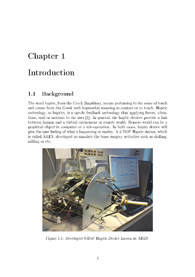
The word haptic, from the Greek (haptikos), means pertaining to the sense of touchand comes from the Greek verb haptesthai meaning to contact or to touch. Haptictechnology, or haptics, is a tactile feedback technology that applying forces, vibra-tions, and/or motions to the user.[1]. In general, the haptic devices provide a linkbetween human and a virtual enviroment or remote world. Remote world can be agraphical object in computer or a tele-operation. In both cases, haptic device willgive the user feeling of what's happening in reality. A 6-DOF Haptic device, whichis called ARES, developed to simulate the bone surgery activities such as drilling,milling or etc.
Figure 1.1: Developed 6-DoF Haptic Device known as ARES
4
CHAPTER 1. INTRODUCTION Control of 6-DoF Haptic Device
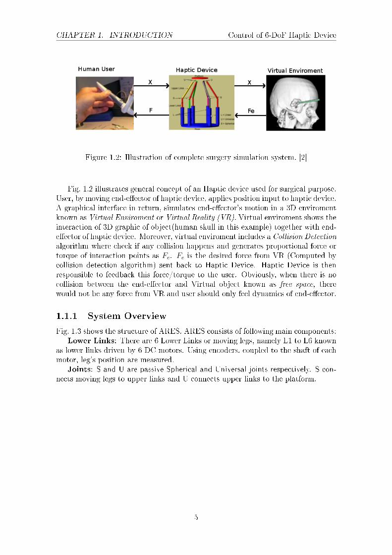
Figure 1.2: Illustration of complete surgery simulation system. [2]
Fig. 1.2 illustrates general concept of an Haptic device used for surgical purpose.User, by moving end-eector of haptic device, applies position input to haptic device.A graphical interface in return, simulates end-eector's motion in a 3D enviromentknown as Virtual Enviroment or Virtual Reality (VR). Virtual enviroment shows theinteraction of 3D graphic of object(human skull in this example) together with end-eector of haptic device. Moreover, virtual enviroment includes a Collision Detectionalgorithm where check if any collision happens and generates proportional force ortorque of interaction points as Fe. Fe is the desired force from VR (Computed bycollision detection algorithm) sent back to Haptic Device. Haptic Device is thenresponsible to feedback this force/torque to the user. Obviously, when there is nocollision between the end-eector and Virtual object known as free space, therewould not be any force from VR and user should only feel dynamics of end-eector.
1.1.1 System Overview
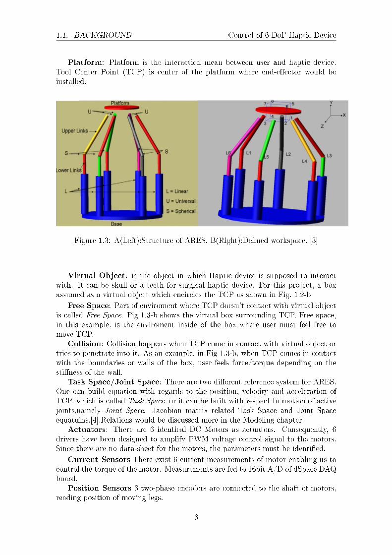
Fig. 1.3 shows the structure of ARES. ARES consists of following main components:Lower Links: There are 6 Lower Links or moving legs, namely L1 to L6 known
as lower links driven by 6 DC motors. Using encoders, coupled to the shaft of eachmotor, leg's position are measured.
Joints: S and U are passive Spherical and Universal joints respectively. S con-nects moving legs to upper links and U connects upper links to the platform.
5
1.1. BACKGROUND Control of 6-DoF Haptic Device
Platform: Platform is the interaction mean between user and haptic device.Tool Center Point (TCP) is center of the platform where end-eector would beinstalled.
Figure 1.3: A(Left):Structure of ARES. B(Right):Dened workspace. [3]
Virtual Object: is the object in which Haptic device is supposed to interactwith. It can be skull or a teeth for surgical haptic device. For this project, a boxassumed as a virtual object which encircles the TCP as shown in Fig. 1.2-b
Free Space: Part of enviroment where TCP doesn't contact with virtual objectis called Free Space. Fig 1.3-b shows the virtual box surrounding TCP. Free space,in this example, is the enviroment inside of the box where user must feel free tomove TCP.
Collision: Collision happens when TCP come in contact with virtual object ortries to penetrate into it. As an example, in Fig 1.3-b, when TCP comes in contactwith the boundaries or walls of the box, user feels force/torque depending on thestiness of the wall.
Task Space/Joint Space: There are two dierent reference system for ARES.One can build equation with regards to the position, velocity and acceleration ofTCP, which is called Task Space, or it can be built with respect to motion of activejoints,namely Joint Space. Jacobian matrix related Task Space and Joint Spaceequatuins.[4].Relations would be discussed more in the Modeling chapter.
Actuators: There are 6 identical DC Motors as actuators. Consequently, 6drivers have been designed to amplify PWM voltage control signal to the motors.Since there are no data-sheet for the motors, the parameters must be identied.
Current Sensors There exist 6 current measurements of motor enabling us tocontrol the torque of the motor. Measurements are fed to 16bit A/D of dSpace DAQboard.
Position Sensors 6 two-phase encoders are connected to the shaft of motors,reading position of moving legs.
6
CHAPTER 1. INTRODUCTION Control of 6-DoF Haptic Device
Hardware and Software Requirement
Matlab and SimulinkdSpace dSpace is a Real-time prototyping hardware in which we implement thecontrol system. After creating control system with Simulink blocks, it will be down-loaded to dSpace. dSpace board used in this project is:rti1103
1.1.2 Problem Description
The aim of this project is to study, partially model,design and implement an appro-priate control system for 6-DoF Haptic device. Dierent control approach will bestudied and then one method will be implemented.
Modeling and Identication
In any control design project, project begins with developing a model of the systemwhich plays an important role for designing an appropriate controller. Since dy-namic model is available for this system([3]) we mostly will focus on identicationof parameters, although dynamic model is nonlinear. We will rst start by a readingand research sub phase. This will mostly consist of reading a set of articles aboutmodeling, identication and control of Haptic. After developing a suciently solidbackground we will be meeting to derive an initial mathematical model with iden-tied parameter that will attempt to correctly describe the dynamics of the device.Validating the model to check whereas our parameters are correctly identied is thelast step of this phase.
Control Design and Implementation
As the core of the project, this phase will be the most enduring one and will proveto be the most challenging. Controller's job can be divided in two main part:
Free Space As illustrated in Fig.1.3-b, TCP is surrounded by a closed boxas an virtual object. ARES should be transparent in free space meaning the usershould not any force/torque while moving TCP inside the box. Transparency isa key performance for haptic devices meaning the user must not feel force/torquefrom dynamic of the device, friction in moving parts or back-EMF of the motors,either in free space or in collision. In other word, haptic should behave in a way thatthe user just feel the end-eector not any other forces/torques mentioned. Then,controller task in this part is just to compensate for friction in moving parts (legmostly), Back EMF of motors and dynamics of the device.
Collision In addition to transparency, which can be done by compensating dy-namic, friction and Back EMF, hand Haptic should exert force/torque to user handwhen they contact with or tries to penetrate into the virtual object. Dependingon the stiness of the virtual object, which is dened by the user, and penetrationdepth collision detection algorithm creates appropriate force/torque which need tobe applied by the haptic device and feedback to the user. As a result, the controllertask in this part is to follow a stepoint or desired value is given from collision detec-tion algorithm along with compensation for friction, dynamics and Back EMF.
7
1.2. REPORT OUTLINE Control of 6-DoF Haptic Device
Although controller doesn't need to have zero steady state error since human sensedoesn't have a exact measure of the force applied, but at least it should be in a waythat the user should feel the virtual reality as if they're touching a same object inthe real world. Following specication of the controller is of high interest and wouldbe investigated:
• A Robustibility and in presence of perturbation and measurement noise.
• C Transparency of device when moving in free space and collision by exactcompensation of device dynamic, friction and Back-EMF.
• C Stability of device in collision.
To do so, dierent controller would be designed, implemented and compared.
1.2 Report outline
Report is divided into some main chapters as followsChapter 1: Introduction First chapter is an introduction to thesis work.
There problem is described, objective of the thesis and appropriate approach tosolve the problem are explained.
Chapter 2: Modeling In this chapter, model of ARES is studied. Since gen-eral model of device is available [4], unidentied components and terms would beidentied.
Chapter 3: Control Design Dierent controller, starting with simplest tomore sophisticated ones are studied and designed. Finally a comparison carried outto show performance of each.
Chapter 4: Implementation Controllers designed in Chapter 3 are discretizedfor implementation.
Chapter 5: Experiments Dierent measurements like current and positionare studied. Limitation of these measurement speed and acceleration estimation areexplored in details. Experimental result and a comparison of the controller also areincluded in this chapter.
Chapter 6: Future Work and Conclusion A summary of thesis along withpossible improvement are presented in this chapter.
8
Chapter 2
Modeling
2.1 Model of ARES
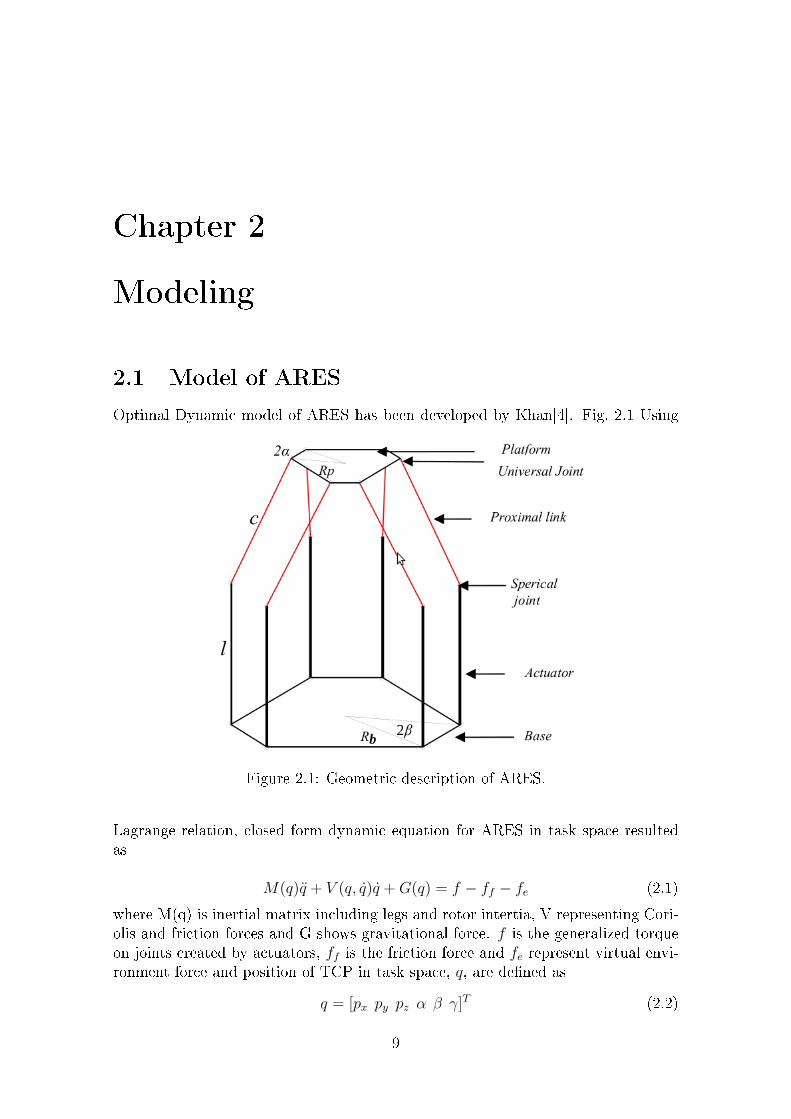
Optimal Dynamic model of ARES has been developed by Khan[4]. Fig. 2.1 Using
Figure 2.1: Geometric description of ARES.
Lagrange relation, closed form dynamic equation for ARES in task space resultedas
M(q)q + V (q, q)q +G(q) = f − ff − fe (2.1)
where M(q) is inertial matrix including legs and rotor intertia, V representing Cori-olis and friction forces and G shows gravitational force. f is the generalized torqueon joints created by actuators, ff is the friction force and fe represent virtual envi-ronment force and position of TCP in task space, q, are dened as
q = [px py pz α β γ]T (2.2)
9
2.1. MODEL OF ARES Control of 6-DoF Haptic Device
q, q, q are the position, velocity and acceleration of TCP respectively. M and Vmatrices 6× 6 and G, f, ff , fe, q, q, q are 6× 1 vectors.
Controllers can be designed in Task space or joint spaces. In task space, we baseequation on the end eector, while in joint space, equation is written with respectto joints. Since current measurment of motor is availble instead of force sensor atthe end eector, joint space control seems to be more suitable.
The resultant generalized force can be converted to torque on the joints usingJacobian Matrix as
τ = J−T (q)f (2.3)
Besides, following equation applies to task/joint spaces conversion[4]
l = Jq (2.4)
l = J (q) + J q (2.5)
where J is Jacobian matrix. l is a vector of size of 1-by-6 indicating the positionof each leg.One can convert encoders tick of motor's shaft to the position of the legby some factor depending on the radius of the pulley. Consequently, l describes thespeed of the legs.Plugging Eq. 2.3 to 2.5 in Eq. 2.1 results following Joint(leg) space dynamic torquebalance equation
M(l)l + V (l, l) +G(l) = τ − τf − τe (2.6)
Where τ is the resultant torque on the joints (motor's shaft),τf is the friction torquein the legs [Section 2.2](friction in the spherical joint are ignored) and τe is computedtorque from virtual reality and is set-point torque need to be followed.
Since control signal of ARES are voltage input to motors, one need to entercontrol signal to the model as well. Following relation describes th relation of τand control signal V , as voltage of motor's terminal. According to schematic 3.2,system would be linearized by adding nonlinear component to control signal. TakingLaplace transform of 2.13 and 2.14 yields
Va = RaIa + LasI +Kbsθ (2.7)
τ = Jts2θ + bsθ → θ =
τ
Jts2 + bs(2.8)
Assuming b=0 and substitude Eq. 2.7 in Eq. 2.8 yields
τ =KtJts
LaJts2 + JtRas+KbKt
Va (2.9)
τi =KtiJtis
LaiJtis2 + JtiRais+KbiKti
Vai, i = 1...6 (2.10)
As a result Eq. 2.6 re-written as
10
CHAPTER 2. MODELING Control of 6-DoF Haptic Device
M(l)l + V (l, l) +G(l) =
Kt1Jt1sLa1Jt1s2+Jt1Ra1s+Kb1Kt1
Va1Kt1Jt2s
La2Jt2s2+Jt2Ra2s+Kb2Kt2Va2
Kt1Jt3sLa3Jt3s2+Jt3Ra3s+Kb3Kt3
Va3Kt1Jt4s
La4Jt4s2+Jt4Ra4s+Kb4Kt4Va4
Kt1Jt5sLa5Jt5s2+Jt5Ra5s+Kb5Kt5
Va5Kt1Jt6s
La6Jt6s2+Jt6Ra6s+Kb6Kt6Va6
− τf − τe (2.11)
Eq. 2.11 is a MIMO model with nonlinear terms which need to be simplied forcontrol purpose. In Section 3.2, feedback linearization method would be discussedto linearize above-mentioned equation. In the Left side of Eq. 2.11, V term is a smallvalue and can be ignored. The other two terms are known and can be calculatednumerically [4]. Assuming τdynamic = M(l)l +G(l) Eq. 2.11 can be written as
Kt1Jt1sLa1Jt1s2+Jt1Ra1s+Kb1Kt1
Va1Kt1Jt2s
La2Jt2s2+Jt2Ra2s+Kb2Kt2Va2
Kt1Jt3sLa3Jt3s2+Jt3Ra3s+Kb3Kt3
Va3Kt1Jt4s
La4Jt4s2+Jt4Ra4s+Kb4Kt4Va4
Kt1Jt5sLa5Jt5s2+Jt5Ra5s+Kb5Kt5
Va5Kt1Jt6s
La6Jt6s2+Jt6Ra6s+Kb6Kt6Va6
= τe +
Nonlinear terms︷ ︸︸ ︷τf + τdynamic
(2.12)
Form Eq. 3.2, τf , friction of moving legs and τ which is a function of control signaland motor parameters, must be identied. Therefor for the rest of this chapter,identication of DC motor and friction are discussed.
2.1.1 Motor Model
There are six DC motor need to be identied. Some parameters of each motorare available but one need to identify the rest. To identify motor's parameters,motors are disconnected from the legs(lower links). Since rotor inertial, Ja , is aknown parameter from the data sheet armature resistor,Ra, motor's inductance, La,and torque constant, Kt,need to be estimated. Experiments carried out along withMatlab Identication Toolbox to identify unknown parameters. In this part frictionof shaft is ignored and we try to identify just motor's parameters. Later frictionparameters would be identied with dierent experiment. Following equations holdfor DC motor
Va = Raia + Ladiadt
+ Vb , Vb = Kbdθ
dt(2.13)
τ = Ktia , τl = Jtθ + bθ , Jt = Ja + Jload (2.14)
where
11
2.1. MODEL OF ARES Control of 6-DoF Haptic Device
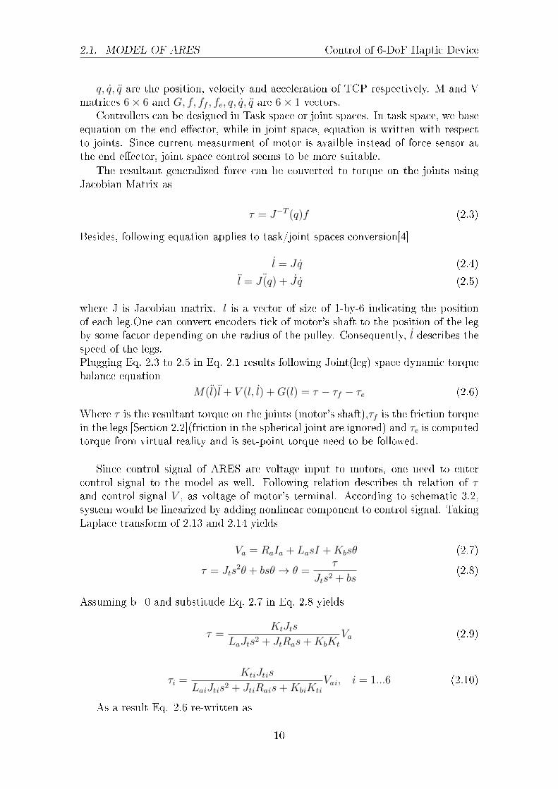
Figure 2.2: Circuit schematic of DC motor.
Va : input voltage [V]Vb : Back-Emf voltage [V]Ra : Armature Resistor [Ω]La : Coil Inductance [H]ia : Armature current [A]θ : angular position [Rad]θ : Angular Speed [ rad
s]
θ : Angular Acceleration [ rads2]
Kt : Motor Torque Constant [N.m/A]Kb : Motor Back EMF [N.m/A]Ja : Rotor inertial [kg.m
2]Jload : Load inertial[kg.m2]Jt : Total inertia [kg.m
2]b : Damping [N.s
m]
τ : Motor Torque [N.m]τl : Load Torque [N.m] :load is just motor's shaftFollowing transfer function concluded from Eq.2.13 and 2.14 which will be used forparameter identication.
θ
Va=
Kt
s(LaJts2 + (JtRa + bLa)s+ bRa +KbKt)(2.15)
Assuming b = 0 yields
θ
Va=
Kt
s(LaJts2 + JtRas+KbKt)(2.16)
Experimental setup
Following experimental schematic shows setup for above-mentioned process. Param-eters shall be identied in open loop.
Appropriate excitation signal is of vital part of identication process. One needsto excite dierent modes of the system to obtain a good estimation . Telegraph signalis used for this purpose. This signal should include both narrow and wide enoughpulses to trigger dierent mode of the system. Required minimum pulse width is
12
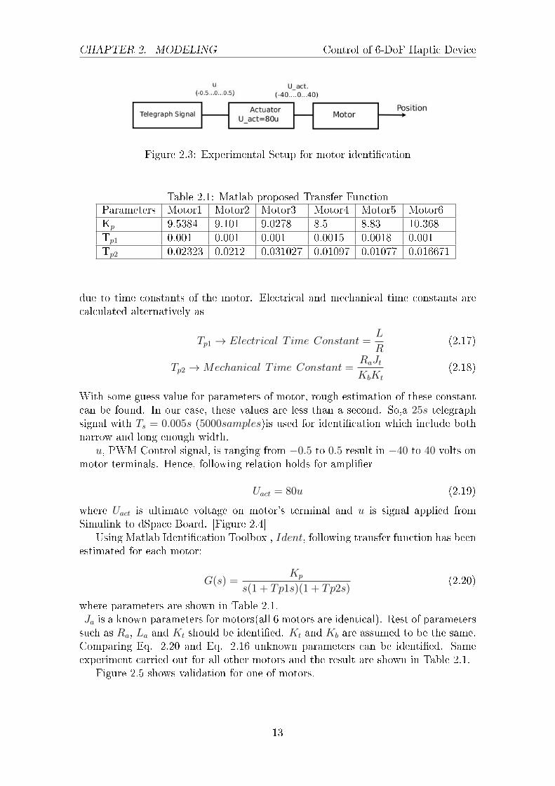
CHAPTER 2. MODELING Control of 6-DoF Haptic Device
Figure 2.3: Experimental Setup for motor identication
Table 2.1: Matlab proposed Transfer FunctionParameters Motor1 Motor2 Motor3 Motor4 Motor5 Motor6Kp 9.5384 9.101 9.0278 8.5 8.83 10.368Tp1 0.001 0.001 0.001 0.0015 0.0018 0.001Tp2 0.02323 0.0212 0.031027 0.01097 0.01077 0.016671
due to time constants of the motor. Electrical and mechanical time constants arecalculated alternatively as
Tp1 → Electrical T ime Constant =L
R(2.17)
Tp2 →Mechanical T ime Constant =RaJtKbKt
(2.18)
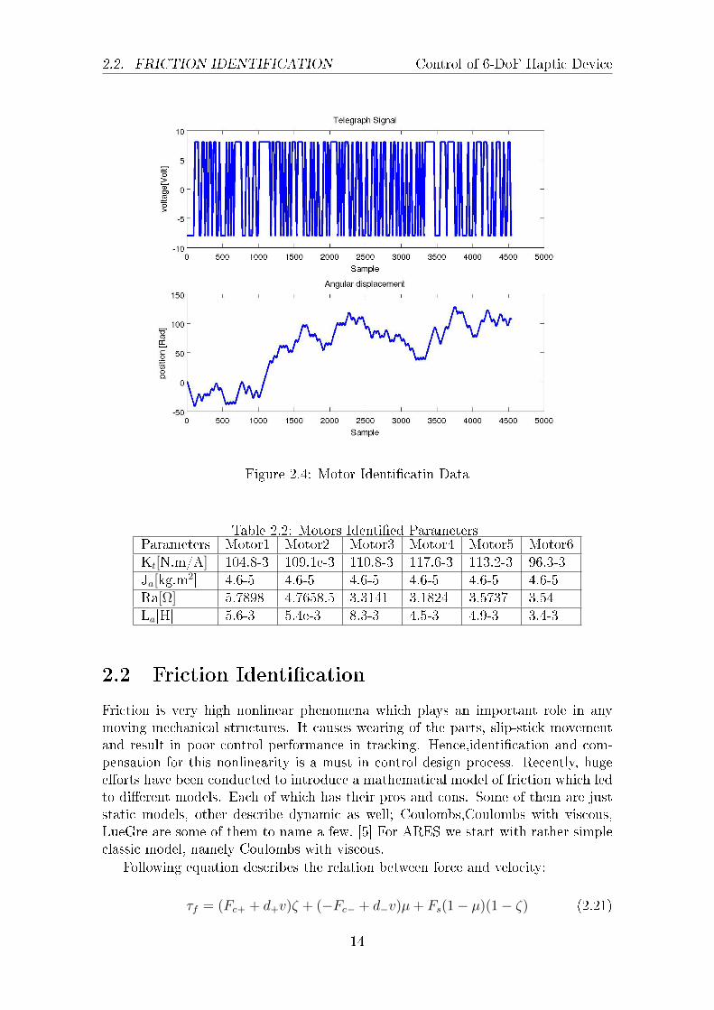
With some guess value for parameters of motor, rough estimation of these constantcan be found. In our case, these values are less than a second. So,a 25s telegraphsignal with Ts = 0.005s (5000samples)is used for identication which include bothnarrow and long enough width.
u, PWM Control signal, is ranging from −0.5 to 0.5 result in −40 to 40 volts onmotor terminals. Hence, following relation holds for amplier
Uact = 80u (2.19)
where Uact is ultimate voltage on motor's terminal and u is signal applied fromSimulink to dSpace Board. [Figure 2.4]
Using Matlab Identication Toolbox , Ident, following transfer function has beenestimated for each motor:
G(s) =Kp
s(1 + Tp1s)(1 + Tp2s)(2.20)
where parameters are shown in Table 2.1.Ja is a known parameters for motors(all 6 motors are identical). Rest of parameterssuch as Ra, La and Kt should be identied. Kt and Kb are assumed to be the same.Comparing Eq. 2.20 and Eq. 2.16 unknown parameters can be identied. Sameexperiment carried out for all other motors and the result are shown in Table 2.1.
Figure 2.5 shows validation for one of motors.
13
2.2. FRICTION IDENTIFICATION Control of 6-DoF Haptic Device
Figure 2.4: Motor Identicatin Data
Table 2.2: Motors Identied ParametersParameters Motor1 Motor2 Motor3 Motor4 Motor5 Motor6Kt[N.m/A] 104.8-3 109.1e-3 110.8-3 117.6-3 113.2-3 96.3-3Ja[kg.m
2] 4.6-5 4.6-5 4.6-5 4.6-5 4.6-5 4.6-5Ra[Ω] 5.7898 4.7658.5 3.3141 3.1824 3.5737 3.54La[H] 5.6-3 5.4e-3 8.3-3 4.5-3 4.9-3 3.4-3
2.2 Friction Identication
Friction is very high nonlinear phenomena which plays an important role in anymoving mechanical structures. It causes wearing of the parts, slip-stick movementand result in poor control performance in tracking. Hence,identication and com-pensation for this nonlinearity is a must in control design process. Recently, hugeeorts have been conducted to introduce a mathematical model of friction which ledto dierent models. Each of which has their pros and cons. Some of them are juststatic models, other describe dynamic as well; Coulombs,Coulombs with viscous,LueGre are some of them to name a few. [5] For ARES we start with rather simpleclassic model, namely Coulombs with viscous.
Following equation describes the relation between force and velocity:
τf = (Fc+ + d+v)ζ + (−Fc− + d−v)µ+ Fs(1− µ)(1− ζ) (2.21)
14
CHAPTER 2. MODELING Control of 6-DoF Haptic Device
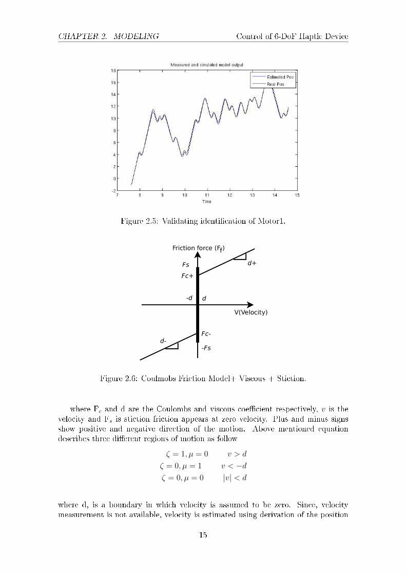
Figure 2.5: Validating identication of Motor1.
Figure 2.6: Coulmobs Friction Model+ Viscous + Stiction.
where Fc and d are the Coulombs and viscous coecient respectively, v is thevelocity and Fs is stiction friction appears at zero velocity. Plus and minus signsshow positive and negative direction of the motion. Above mentioned equationdescribes three dierent regions of motion as follow
ζ = 1, µ = 0 v > d
ζ = 0, µ = 1 v < −dζ = 0, µ = 0 |v| < d
where d, is a boundary in which velocity is assumed to be zero. Since, velocitymeasurement is not available, velocity is estimated using derivation of the position
15
2.2. FRICTION IDENTIFICATION Control of 6-DoF Haptic Device
measurement. Discontinuity in position measurement (tick of encoder are convertedto position of the shaft) causes some dierentiation error. Apply a bound as zerovelocity is a remedy for this problem.
2.2.1 Friction Model
To identify friction model in Eq. 2.21, Fc+ , Fc− , d+ and d− are four parametersshould be identied through some estimation method. Fs, static friction, can becalculated experimentally. To estimate Coulombs and viscous parameters we needto perform an experiment with velocity as a reference signal and measure frictionforce as an output. In general, following torque balance can be considered for DCmotor
τ = τt + τf (2.22)
where τ is motor torque generated by the current, τt is total torque including loadand inertial torque and τf is friction torque projected on motor's shaft includingshaft friction and moving leg. Equation 2.22 can be written as:
Kti = Jtθ + τf (2.23)
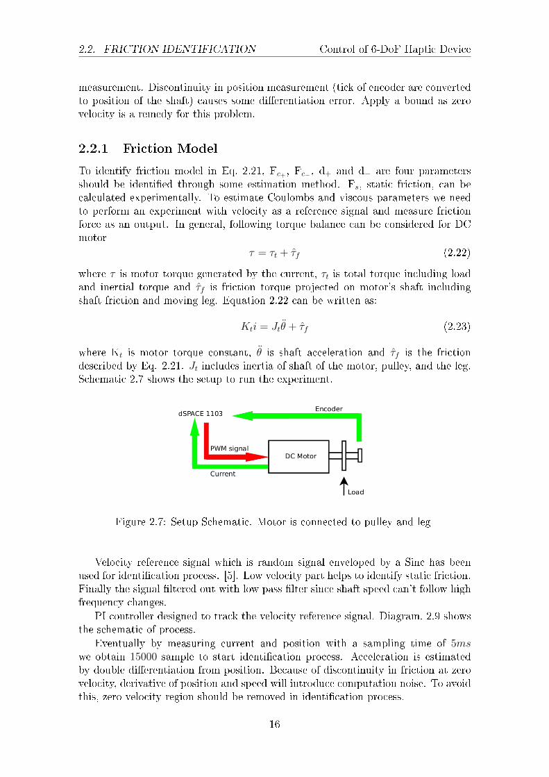
where Kt is motor torque constant, θ is shaft acceleration and τf is the frictiondescribed by Eq. 2.21. Jt includes inertia of shaft of the motor, pulley, and the leg.Schematic 2.7 shows the setup to run the experiment.
Figure 2.7: Setup Schematic. Motor is connected to pulley and leg
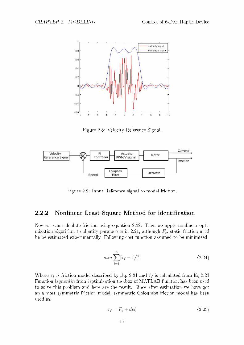
Velocity reference signal which is random signal enveloped by a Sinc has beenused for identication process. [5]. Low velocity part helps to identify static friction.Finally the signal ltered out with low pass lter since shaft speed can't follow highfrequency changes.
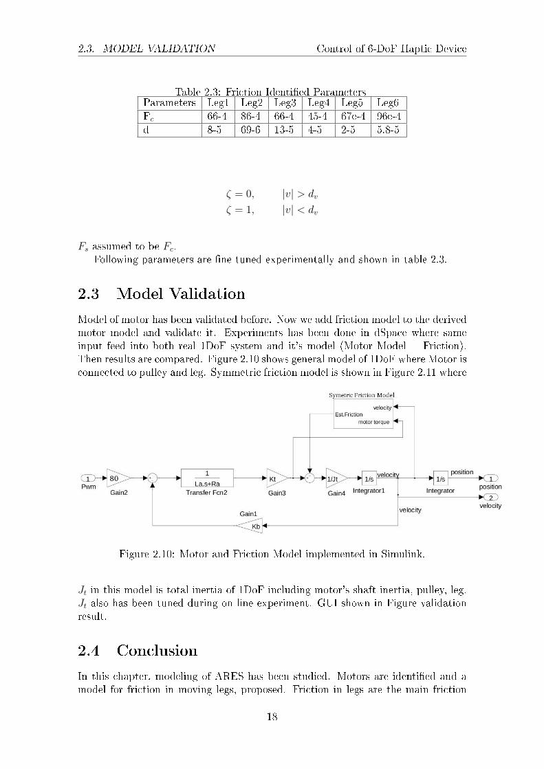
PI controller designed to track the velocity reference signal. Diagram. 2.9 showsthe schematic of process.
Eventually by measuring current and position with a sampling time of 5mswe obtain 15000 sample to start identication process. Acceleration is estimatedby double dierentiation from position. Because of discontinuity in friction at zerovelocity, derivative of position and speed will introduce computation noise. To avoidthis, zero velocity region should be removed in identication process.
16
CHAPTER 2. MODELING Control of 6-DoF Haptic Device
Figure 2.8: Velocity Reference Signal.
Figure 2.9: Input Reference signal to model friction.
2.2.2 Nonlinear Least Square Method for identication
Now we can calculate friction using equation 2.22. Then we apply nonlinear opti-mization algorithm to identify parameters in 2.21, although Fs, static friction needbe be estimated experimentally. Following cost function assumed to be minimized
min
n∑i=1
[τf − τf ]2; (2.24)
Where τf is friction model described by Eq. 2.21 and τf is calculated from Eq.2.23Function lsqnonlin from Optimization toolbox of MATLAB function has been usedto solve this problem and here are the result. Since after estimation we have gotan almost symmetric friction model, symmetric Coloumbs friction model has beenused as.
τf = Fc + dvζ (2.25)
17
2.3. MODEL VALIDATION Control of 6-DoF Haptic Device
Table 2.3: Friction Identied ParametersParameters Leg1 Leg2 Leg3 Leg4 Leg5 Leg6Fc 66-4 86-4 66-4 45-4 67e-4 96e-4d 8-5 69-6 13-5 4-5 2-5 5.8-5
ζ = 0, |v| > dv
ζ = 1, |v| < dv
Fs assumed to be Fc.Following parameters are ne tuned experimentally and shown in table 2.3.
2.3 Model Validation
Model of motor has been validated before. Now we add friction model to the derivedmotor model and validate it. Experiments has been done in dSpace where sameinput feed into both real 1DoF system and it's model (Motor Model + Friction).Then results are compared. Figure 2.10 shows general model of 1DoF where Motor isconnected to pulley and leg. Symmetric friction model is shown in Figure 2.11 where
Figure 2.10: Motor and Friction Model implemented in Simulink.
Jt in this model is total inertia of 1DoF including motor's shaft inertia, pulley, leg.Jt also has been tuned during on line experiment. GUI shown in Figure validationresult.
2.4 Conclusion
In this chapter, modeling of ARES has been studied. Motors are identied and amodel for friction in moving legs, proposed. Friction in legs are the main friction
18
CHAPTER 2. MODELING Control of 6-DoF Haptic Device
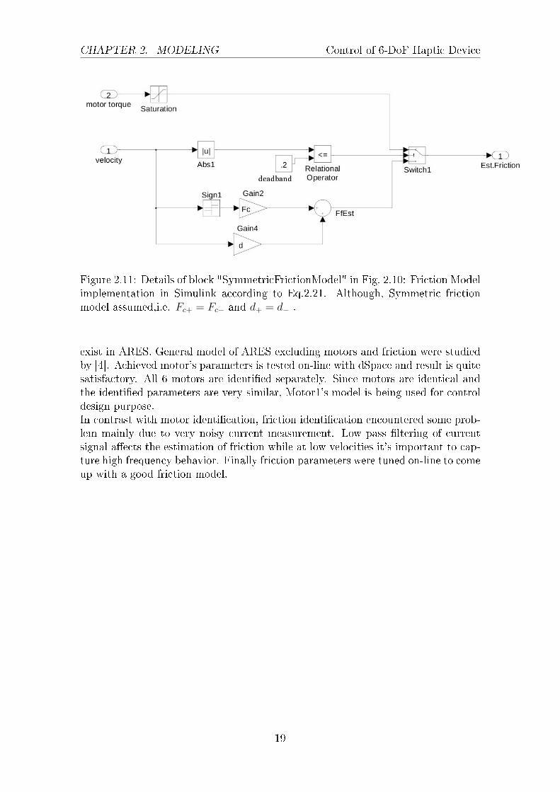
Figure 2.11: Details of block "SymmetricFrictionModel" in Fig. 2.10: Friction Modelimplementation in Simulink according to Eq.2.21. Although, Symmetric frictionmodel assumed,i.e. Fc+ = Fc− and d+ = d− .
exist in ARES. General model of ARES excluding motors and friction were studiedby [4]. Achieved motor's parameters is tested on-line with dSpace and result is quitesatisfactory. All 6 motors are identied separately. Since motors are identical andthe identied parameters are very similar, Motor1's model is being used for controldesign purpose.In contrast with motor identication, friction identication encountered some prob-lem mainly due to very noisy current measurement. Low pass ltering of currentsignal aects the estimation of friction while at low velocities it's important to cap-ture high frequency behavior. Finally friction parameters were tuned on-line to comeup with a good friction model.
19
2.4. CONCLUSION Control of 6-DoF Haptic Device
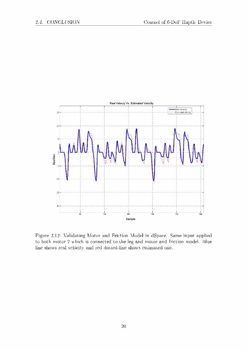
Figure 2.12: Validating Motor and Friction Model in dSpace. Same input appliedto both motor 2 which is connected to the leg and motor and friction model. Blueline shows real velocity and red dotted-line shows estimated one.
20
Chapter 3
Control Design
3.1 Introduction
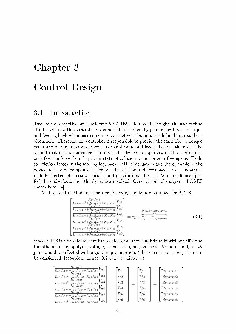
Two control objective are considered for ARES. Main goal is to give the user feelingof interaction with a virtual environment.This is done by generating force or torqueand feeding back when user come into contact with boundaries dened in virtual en-vironment. Therefore the controller is responsible to provide the same Force/Torquegenerated by virtual environment as desired value and feed it back to the user. Thesecond task of the controller is to make the device transparent, i.e the user shouldonly feel the force from haptic in state of collision or no force in free space. To doso, friction forces in the moving leg, back EMF of actuators and the dynamic of thedevice need to be compensated for both in collision and free space states. Dynamicsinclude inertial of masses, Coriolis and gravitational forces. As a result user justfeel the end-eector not the dynamics involved. General control diagram of ARESshown here. [4]
As discussed in Modeling chapter, following model are assumed for ARES.
Kt1Jt1sLa1Jt1s2+Jt1Ra1s+Kb1Kt1
Va1Kt1Jt2s
La2Jt2s2+Jt2Ra2s+Kb2Kt2Va2
Kt1Jt3sLa3Jt3s2+Jt3Ra3s+Kb3Kt3
Va3Kt1Jt4s
La4Jt4s2+Jt4Ra4s+Kb4Kt4Va4
Kt1Jt5sLa5Jt5s2+Jt5Ra5s+Kb5Kt5
Va5Kt1Jt6s
La6Jt6s2+Jt6Ra6s+Kb6Kt6Va6
= τe +
Nonlinear terms︷ ︸︸ ︷τf + τdynamic (3.1)
Since ARES is a parallel mechanism, each leg can move individually without aectingthe others, i.e. by applying voltage, as control signal, on the i−th motor, only i−thjoint would be aected with a good approximation. This means that the system canbe considered decoupled. Hence 3.2 can be written as
Kt1Jt1sLa1Jt1s2+Jt1Ra1s+Kb1Kt1
Va1Kt1Jt2s
La2Jt2s2+Jt2Ra2s+Kb2Kt2Va2
Kt1Jt3sLa3Jt3s2+Jt3Ra3s+Kb3Kt3
Va3Kt1Jt4s
La4Jt4s2+Jt4Ra4s+Kb4Kt4Va4
Kt1Jt5sLa5Jt5s2+Jt5Ra5s+Kb5Kt5
Va5Kt1Jt6s
La6Jt6s2+Jt6Ra6s+Kb6Kt6Va6
=
τe1τe2τe3τe4τe5τe6
+
τf1
τf2
τf3
τf4
τf5
τf6
+
τdynamic1τdynamic2τdynamic3τdynamic4τdynamic5τdynamic6
21
3.2. FEEDBACK LINEARIZATION Control of 6-DoF Haptic Device
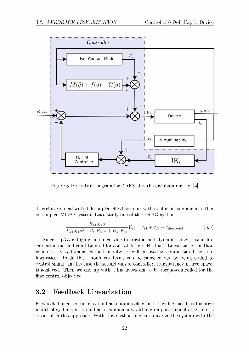
Figure 3.1: Control Diagram for ARES. J is the Jacobian matrix. [4]
Therefor, we deal with 6 decoupled SISO systems with nonlinear component ratheran coupled MIMO system. Let's study one of these SISO system
Kt1Jt1s
La1Jt1s2 + Jt1Ra1s+Kb1Kt1
Va1 = τe1 + τf1 + τdynamic1 (3.3)
Since Eq.3.3 is highly nonlinear due to friction and dynamics itself, usual lin-earization method can't be used for control design. Feedback Linearization methodwhich is a very famous method in robotics will be used to compensated for non-linearities. To do this , nonlinear terms can be canceled out by being added tocontrol signal. In this case the second aim of controller, transparency in free space,is achieved. Then we end up with a linear system to be torque-controlled for therst control objective.
3.2 Feedback Linearization
Feedback Linearization is a nonlinear approach which is widely used to linearizemodel of systems with nonlinear components, although a good model of system isessential in this approach. With this method one can linearize the system with the
22
CHAPTER 3. CONTROL DESIGN Control of 6-DoF Haptic Device
control signal. This method is completely dierent with conventional (Jacobian) lin-earization, because feedback linearization is achieved by exact state transformationand feedback rather than by linear approximation of the dynamics[6].
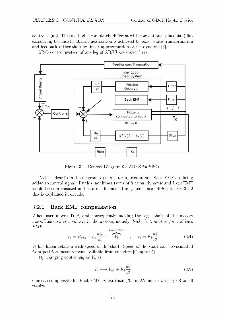
SISO control system of one leg of ARES are shown here.
Figure 3.2: Control Diagram for ARES for SISO.
As it is clear from the diagram, dynamic term, friction and Back EMF are beingadded to control signal. By this, nonlinear terms of friction, dynamic and Back EMFwould be compensated and as a result makes the system linear SISO. In, Sec.3.2.2this is explained in details.
3.2.1 Back EMF compensation
When user moves TCP, and consequently moving the legs, shaft of the motorsmove.This creates a voltage in the motors, namely back electromotive force of backEMF.
Va = Raia + Ladiadt
+
BackEMF︷︸︸︷Vb , Vb = Kb
dθ
dt(3.4)
Vb has linear relation with speed of the shaft. Speed of the shaft can be estimatedfrom position measurement available from encoders.[Chapter 5]
By changing control signal,Va as
Va 7−→ Va1 +Kbdθ
dt(3.5)
One can compensate for Back EMF. Substituting 3.5 in 2.7 and re-writing 2.8 to 2.9results
23
3.2. FEEDBACK LINEARIZATION Control of 6-DoF Haptic Device
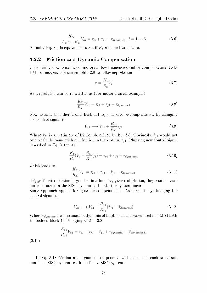
Kti
Lais+Rai
Vai = τei + τfi + τdynamici, i = 1 · · · 6 (3.6)
Actually Eq. 3.6 is equivalent to 3.3 if Kb assumed to be zero.
3.2.2 Friction and Dynamic Compensation
Considering slow dynamics of motors at low frequencies and by compensating Back-EMF of motors, one can simplify 2.9 to following relation
τ =Kt
Ra
Va (3.7)
As a result 3.3 can be re-written as (For motor 1 as an example)
Kt1
Ra1
Va1 = τe1 + τf1 + τdynamic1 (3.8)
Now, assume that there's only friction torque need to be compensated. By changingthe control signal to
Va1 7−→ Va1 +Ra1
Kt1
τf1 (3.9)
Where τf1 is an estimate of friction described by Eq. 3.8. Obviuosly, τf1 would notbe exactly the same with real friction in the system, τf1. Plugging new control signaldescribed in Eq. 3.9 in 3.8
Kt
Ra
(Va +Ra
Kt
τf1) = τe1 + τf1 + τdynamic1 (3.10)
which leads toKt1
Ra1
Va1 = τe1 + τf1 − τf1 + τdynamic1 (3.11)
if τf1,estimated friction, is good estimation of τf1, the real friction, they would cancelout each other in the SISO system and make the system linear.Same approach applies for dynamic compensation. As a result, by changing thecontrol signal to
Va1 7−→ Va1 +Ra1
Kt1
(τf1 + τdynamic) (3.12)
Where τdynamic is an estimate of dynamic of haptic which is calculated in a MATLABEmbedded block[4]. Plunging 3.12 in 3.8
Kt1
Ra1
Va1 = τe1 + τf1 − τf1 + τdynamic1 − τdynamicsf1
(3.13)
In Eq. 3.13 friction and dynamic components will cancel out each other andnonlinear SISO system results in linear SISO system.
24
CHAPTER 3. CONTROL DESIGN Control of 6-DoF Haptic Device
With a good model for Friction, dynamic compensation and Back EMF andaccording to discussion in Sections 3.2.1 and 3.2.2 and selecting control signal as
Vai 7−→ Vai +Kbdθ
dt+Rai
Kti
(τfi + τdynamici) (3.14)
Eq. 3.6 together with 2.19 result in
Gnom =τeiui
=80Kti
Lais+Rai
i = 1 · · · 6 (3.15)
Where Gnom is nominal model of the system if perfect compensation happens whichis not the case in reality. That's why perturbation and robust controller will bediscussed. Gain 80 in the numerator is related to amplier gain converting PWMcontrol signal,u, to motor terminal voltage,Va By selecting control signal in Eq. 3.14we cancel out nonlinearities, make the system down to linear system transparentand as result one of main objective of the controller would be satised where weneed to track torque set points coming from virtual reality, Gnom, Nominal Model ofmotors would be used for control design. For the rst objective, two general controlapproach can be taken:
Unied Controller In both Collision and Free Space controller will trackτe from virtual reality. Since, τe is zero in free space, controller doesn't make anycontrol signal and in the case of collision, taue would be followed by controller. Thisidea is used for control design. Although this approach would be much stable ifcurrent feedback is accurate otherwise user will fee some kicky-motion in free space.
Divide Control tasks Since there are two region namely, Collision and FreeSpace, ARES doesn't need to track any torque from virtual reality in free space,one can turn o the controller at this region and control signal is just compensationterm described by Eq. 3.14. In the other hand controller need to be on when itsupposed to track torque setpoint ,τe from virtual reality. By this, one can eliminateinstability problem happens in free space when rst method is used. Drawback ofthis method is Bumpless transfer which should be taken care of during switching.
3.3 Perturbation
There are six identical motors in ARES,although there are small dierence betweenmotor's parameters. At rst glance motor's parameters may seem dierent whileplotting bode diagram of each motor verify that there are very small dierences.Hence, For the control design, motor1's parameters would be used. In other hand,identication process for motors was quite good, so we don't consider any pertur-bation for motor's parameter.
One of the most important perturbation in haptic device is the user hand. Sincein this project, hand's dynamic has been ignored, it's uncertainty should be consid-ered in some way. Also, there are some over or under compensation which can enterperturbation to system that can be projected on Kb. For jerky hand motion, back
25
3.3. PERTURBATION Control of 6-DoF Haptic Device
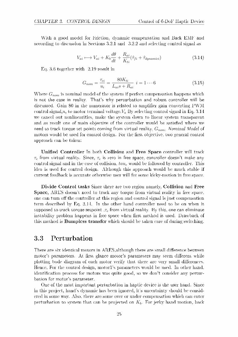
EMF can't be compensated properly. This perturbation can be modeled assumingKb : 0...Kb. Fig. 3.3 shows this perturbation.
Figure 3.3: Perturbed system with Kb: 0 to Kb, By Kb=0 we ignore hand dynamicscompletely and consider it as a sti object
Small variation of velocity can be modeled with Kb parameter and then robustcontroller can be designed to take care of it.
3.3.1 Model Uncertainties
So far, we focus on nominal model(Eq. 3.15) of the system. Although there are vari-ous model errors result in a dierent closed loop system than expected. Consideringthe true system as Gperturbation following relation is assumed between Gperturbed andGnom
Gperturbed = (I + ∆G)Gnom (3.16)
where ∆G is the model error. For rest of this report term G would be used insteadof Gnom, unless it's mentioned. Finally Gperturbation is modeled as
Gperturbed =80KtiJtis
LaiJtis2 + JtiRais+KbiKti
Vai (3.17)
Where Kb = 0...Kb.So far, We showed that how one can break down nonlinear MIMO control of
ARES problem to a simple linear SISO problem. In addition to transparency forboth collision or free space, which was done by adding term to control signal, tracking
26
CHAPTER 3. CONTROL DESIGN Control of 6-DoF Haptic Device
setpoint from virtual enviroment τe is another control task. From now on, we focuson control design for SISO system with the model described in 3.6. For simplicity,notation i as motor's or leg's number would be dropped.
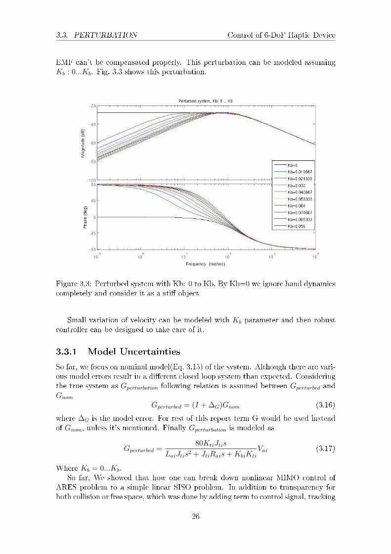
3.4 PI Torque Control
In this section, we analyze PI control for decoupled and simplied model. Thenominal model of the plant is
τeu
=80Kt
Las+Ra
(3.18)
Since control signal,u, is a PWM signal not Va,voltage of motor's terminal, we needto consider this gain to the model.
Figure 3.4: PI Control schematic.
Loop gain of the system, L(s), is
L(s) =Kps+Ki
s
80Kt
Ra + Las
the closed loop transfer-function from R and D to output Y is
Y (s) =40KtKps+ 80KtKi
Las2 + (Ra + 40KtKp)s+ 80KtKp
R(s)+Kts
Las2 + (Ra + 80KtKp)s+ 80KtKp
D(s)
(3.19)And the characteristic equation is
CE : Las2 + (Ra + 80KtKp)s+ 80KtKp (3.20)
That's a second order system with two controller parameter Ki and Kp which canplace the closed loop poles at arbitrary location. Comparing with nominal (ζ,ωn)parameterization
CE : s2 + 2ζωns+ ω2n
27
3.4. PI TORQUE CONTROL Control of 6-DoF Haptic Device
Kp and Ki are
Ki =ω2nLa
80Kt
Kp =2ζωnLa −Ra
80Kt
(3.21)
Since controller need to track torque from virtual reality and that is changing fast,fast response is required. Typical value can be Ts = 0.01. Since it not possibleto achieve it with PI control due to big value Ki which cause instability, we takesettling time, Ts = 0.04s and Maximum Peak Overshoot,MPO < 10%
Ts = 4ζωn
MPO = 100e−ζπ√(1−ζ2)
(3.22)
Ts = 4
ζωn
MPO = 100e−ζπ√(1−ζ2)
⇒
ζ = 0.7
ωn = 142.8
Plugging in Eq.3.21 results Kp = 0.023
Ki = 32.9(3.23)
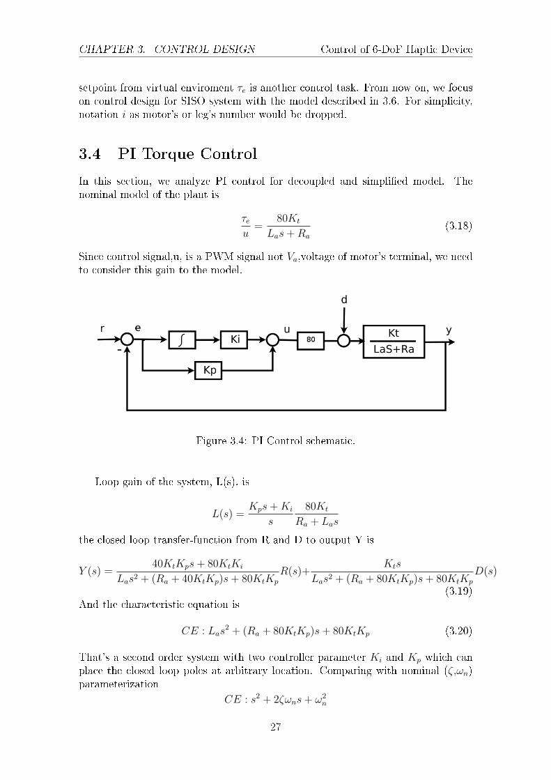
Step response of the system is
Figure 3.5: Step response of close loop system with PI controller.
As that's clear from step response of disturbance we have good disturbancerejection for step input.
28
CHAPTER 3. CONTROL DESIGN Control of 6-DoF Haptic Device
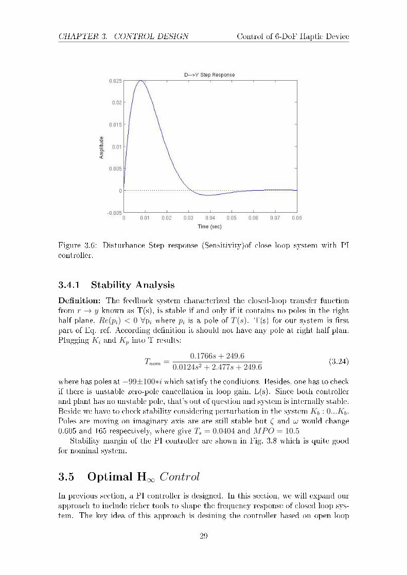
Figure 3.6: Disturbance Step response (Sensitivity)of close loop system with PIcontroller.
3.4.1 Stability Analysis
Denition: The feedback system characterized the closed-loop transfer functionfrom r → y known as T(s), is stable if and only if it contains no poles in the righthalf plane, Re(pi) < 0 ∀pi where pi is a pole of T (s). T(s) for our system is rstpart of Eq. ref. According denition it should not have any pole at right half plan.Plugging Ki and Kp into T results;
Tnom =0.1766s+ 249.6
0.0124s2 + 2.477s+ 249.6(3.24)
where has poles at−99±100∗i which satisfy the conditions. Besides, one has to checkif there is unstable zero-pole cancellation in loop gain, L(s). Since both controllerand plant has no unstable pole, that's out of question and system is internally stable.Beside we have to check stability considering perturbation in the system Kb : 0...Kb.Poles are moving on imaginary axis are are still stable but ζ and ω would change0.605 and 165 respectively, where give Ts = 0.0404 and MPO = 10.5
Stability margin of the PI controller are shown in Fig. 3.8 which is quite goodfor nominal system.
3.5 Optimal H∞ Control
In previous section, a PI controller is designed. In this section, we will expand ourapproach to include richer tools to shape the frequency response of closed loop sys-tem. The key idea of this approach is desining the controller based on open loop
29
3.5. OPTIMAL H∞ CONTROL Control of 6-DoF Haptic Device
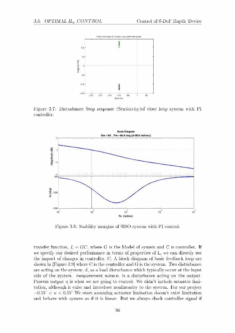
Figure 3.7: Disturbance Step response (Sensitivity)of close loop system with PIcontroller.
Figure 3.8: Stability margins of SISO system with PI control.
transfer function, L = GC, where G is the Model of system and C is controller. Ifwe specify our desired performance in terms of properties of L, we can directly seethe impact of changes in controller, C. A block diagram of basic feedback loop areshown in [Figure 3.9] where C is the controller and G is the system. Two disturbanceare acting on the system, d, as a load disturbance which typically occur at the inputside of the system. measurement noise,n, is a disturbance acting on the output.Process output η is what we are going to control. We didn't include actuator limi-tation, although it exist and introduce nonlinearity to the system. For our project−0.5V < u < 0.5V We start assuming actuator limitation doesn't exist limitationand behave with system as if it is linear. But we always check controller signal if
30
CHAPTER 3. CONTROL DESIGN Control of 6-DoF Haptic Device
it cross the limits. Torque set point,r, also is in the range of −0.2 < r < 0.2. The
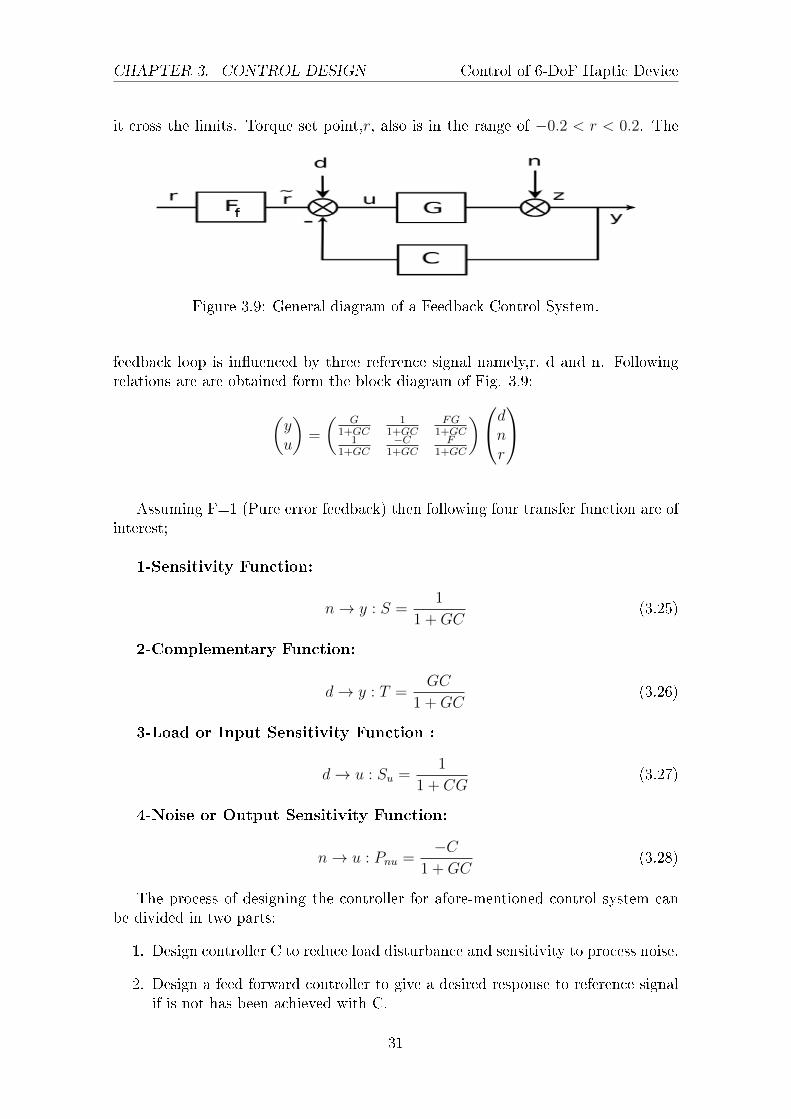
Figure 3.9: General diagram of a Feedback Control System.
feedback loop is inuenced by three reference signal namely,r, d and n. Followingrelations are are obtained form the block diagram of Fig. 3.9:
(yu
)=
(G
1+GC1
1+GCFG
1+GC1
1+GC−C
1+GCF
1+GC
)dnr
Assuming F=1 (Pure error feedback) then following four transfer function are ofinterest;
1-Sensitivity Function:
n→ y : S =1
1 +GC(3.25)
2-Complementary Function:
d→ y : T =GC
1 +GC(3.26)
3-Load or Input Sensitivity Function :
d→ u : Su =1
1 + CG(3.27)
4-Noise or Output Sensitivity Function:
n→ u : Pnu =−C
1 +GC(3.28)
The process of designing the controller for afore-mentioned control system canbe divided in two parts:
1. Design controller C to reduce load disturbance and sensitivity to process noise.
2. Design a feed forward controller to give a desired response to reference signalif is not has been achieved with C.
31
3.5. OPTIMAL H∞ CONTROL Control of 6-DoF Haptic Device
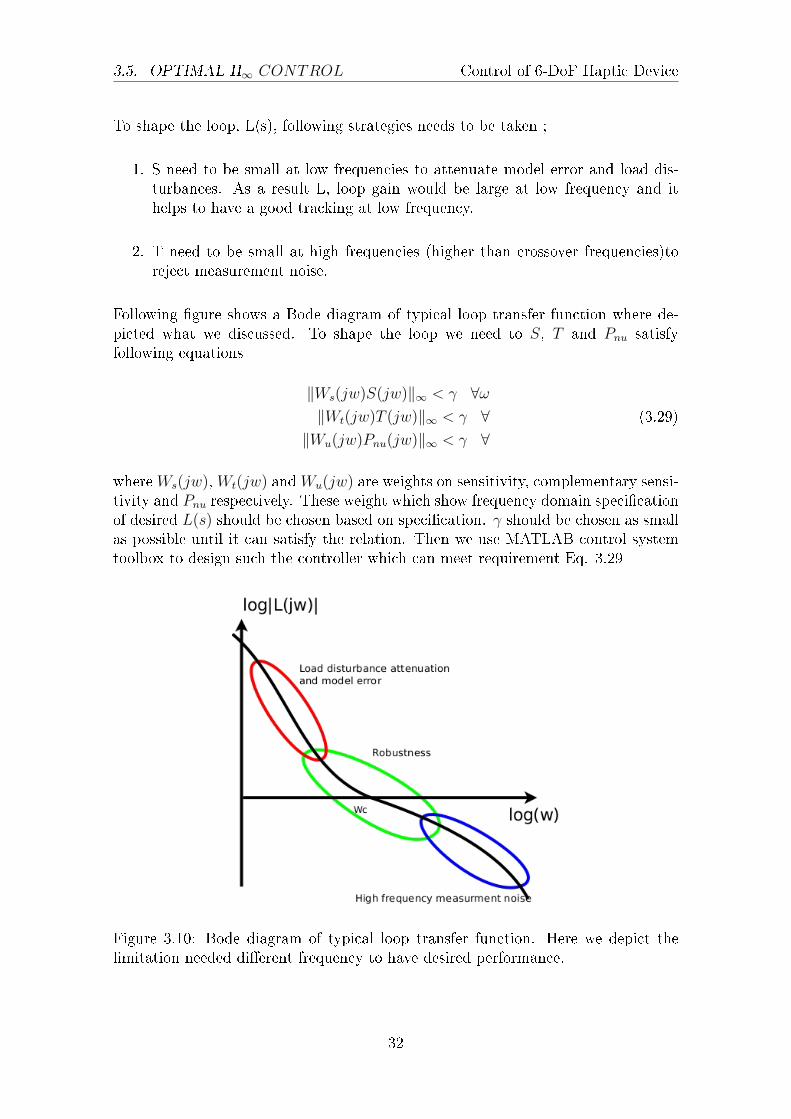
To shape the loop, L(s), following strategies needs to be taken ;
1. S need to be small at low frequencies to attenuate model error and load dis-turbances. As a result L, loop gain would be large at low frequency and ithelps to have a good tracking at low frequency.
2. T need to be small at high frequencies (higher than crossover frequencies)toreject measurement noise.
Following gure shows a Bode diagram of typical loop transfer function where de-picted what we discussed. To shape the loop we need to S, T and Pnu satisfyfollowing equations
‖Ws(jw)S(jw)‖∞ < γ ∀ω‖Wt(jw)T (jw)‖∞ < γ ∀‖Wu(jw)Pnu(jw)‖∞ < γ ∀
(3.29)
whereWs(jw),Wt(jw) andWu(jw) are weights on sensitivity, complementary sensi-tivity and Pnu respectively. These weight which show frequency domain specicationof desired L(s) should be chosen based on specication. γ should be chosen as smallas possible until it can satisfy the relation. Then we use MATLAB control systemtoolbox to design such the controller which can meet requirement Eq. 3.29
Figure 3.10: Bode diagram of typical loop transfer function. Here we depict thelimitation needed dierent frequency to have desired performance.
32
CHAPTER 3. CONTROL DESIGN Control of 6-DoF Haptic Device
3.5.1 Choose Weights
W−1s
Ws need to be small at low frequency. By putting two zero close to origin for W−1s
we make sure to attenuate disturbance and reject model error as much as possible.Of course the best choice is to put poles at zero for Ws. But one need to nd thecontroller which can satisfy all Ws,Wt and Wu. Following weights are chosen:
|W−1s (jω)| = (s+ 1)2
10(3.30)
W−1t
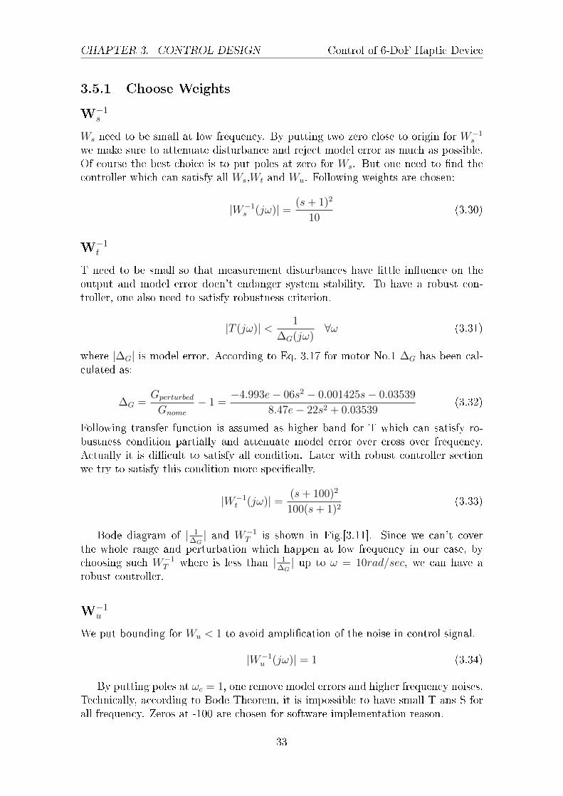
T need to be small so that measurement disturbances have little inuence on theoutput and model error doen't endanger system stability. To have a robust con-troller, one also need to satisfy robustness criterion.
|T (jω)| < 1
∆G(jω)∀ω (3.31)
where |∆G| is model error. According to Eq. 3.17 for motor No.1 ∆G has been cal-culated as:
∆G =Gperturbed
Gnome
− 1 =−4.993e− 06s2 − 0.001425s− 0.03539
8.47e− 22s2 + 0.03539(3.32)
Following transfer function is assumed as higher band for T which can satisfy ro-bustness condition partially and attenuate model error over cross over frequency.Actually it is dicult to satisfy all condition. Later with robust controller sectionwe try to satisfy this condition more specically.
|W−1t (jω)| = (s+ 100)2
100(s+ 1)2(3.33)
Bode diagram of | 1∆G| and W−1
T is shown in Fig.[3.11]. Since we can't coverthe whole range and perturbation which happen at low frequency in our case, bychoosing such W−1
T where is less than | 1∆G| up to ω = 10rad/sec, we can have a
robust controller.
W−1u
We put bounding for Wu < 1 to avoid amplication of the noise in control signal.
|W−1u (jω)| = 1 (3.34)
By putting poles at ωc = 1, one remove model errors and higher frequency noises.Technically, according to Bode Theorem, it is impossible to have small T ans S forall frequency. Zeros at -100 are chosen for software implementation reason.
33
3.5. OPTIMAL H∞ CONTROL Control of 6-DoF Haptic Device
Figure 3.11: Upper bound for T, W−1t , and 1
∆Gare shown. For robustness 1
∆Gshould
be less than W−1t , although it can't satised for all frequency.
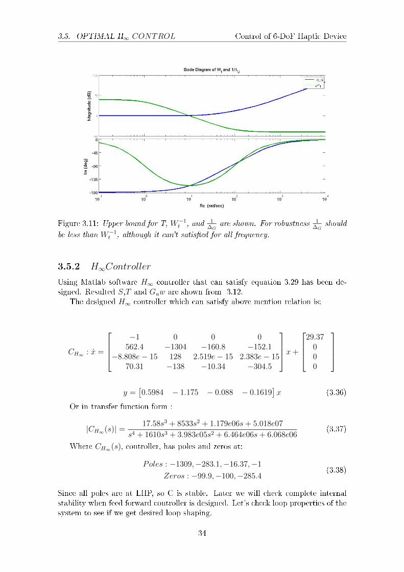
3.5.2 H∞Controller
Using Matlab software H∞ controller that can satisfy equation 3.29 has been de-signed. Resulted S,T and Guw are shown from 3.12.
The designed H∞ controller which can satisfy above mention relation is:
CH∞ : x =
−1 0 0 0
562.4 −1304 −160.8 −152.1−8.808e− 15 128 2.519e− 15 2.383e− 15
70.31 −138 −10.34 −304.5
x+
29.37
000
y =
[0.5984 − 1.175 − 0.088 − 0.1619
]x (3.36)
Or in transfer function form :
|CH∞(s)| = 17.58s3 + 8533s2 + 1.179e06s+ 5.018e07
s4 + 1610s3 + 3.983e05s2 + 6.464e06s+ 6.068e06(3.37)
Where CH∞(s), controller, has poles and zeros at:
Poles : −1309,−283.1,−16.37,−1
Zeros : −99.9,−100,−285.4(3.38)
Since all poles are at LHP, so C is stable. Later we will check complete internalstability when feed forward controller is designed. Let's check loop properties of thesystem to see if we get desired loop shaping.
34
CHAPTER 3. CONTROL DESIGN Control of 6-DoF Haptic Device
Figure 3.12: W−1s ,W−1
t ,W−1u .
35
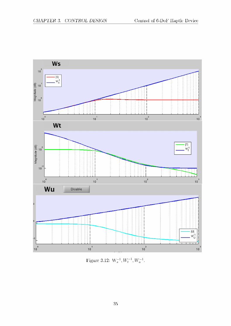
3.5. OPTIMAL H∞ CONTROL Control of 6-DoF Haptic Device
Figure 3.13: Designed Controller. Loop gain, T and S are shown. High negativeslope of L after w = 10 reduces measurement noise dramatically.
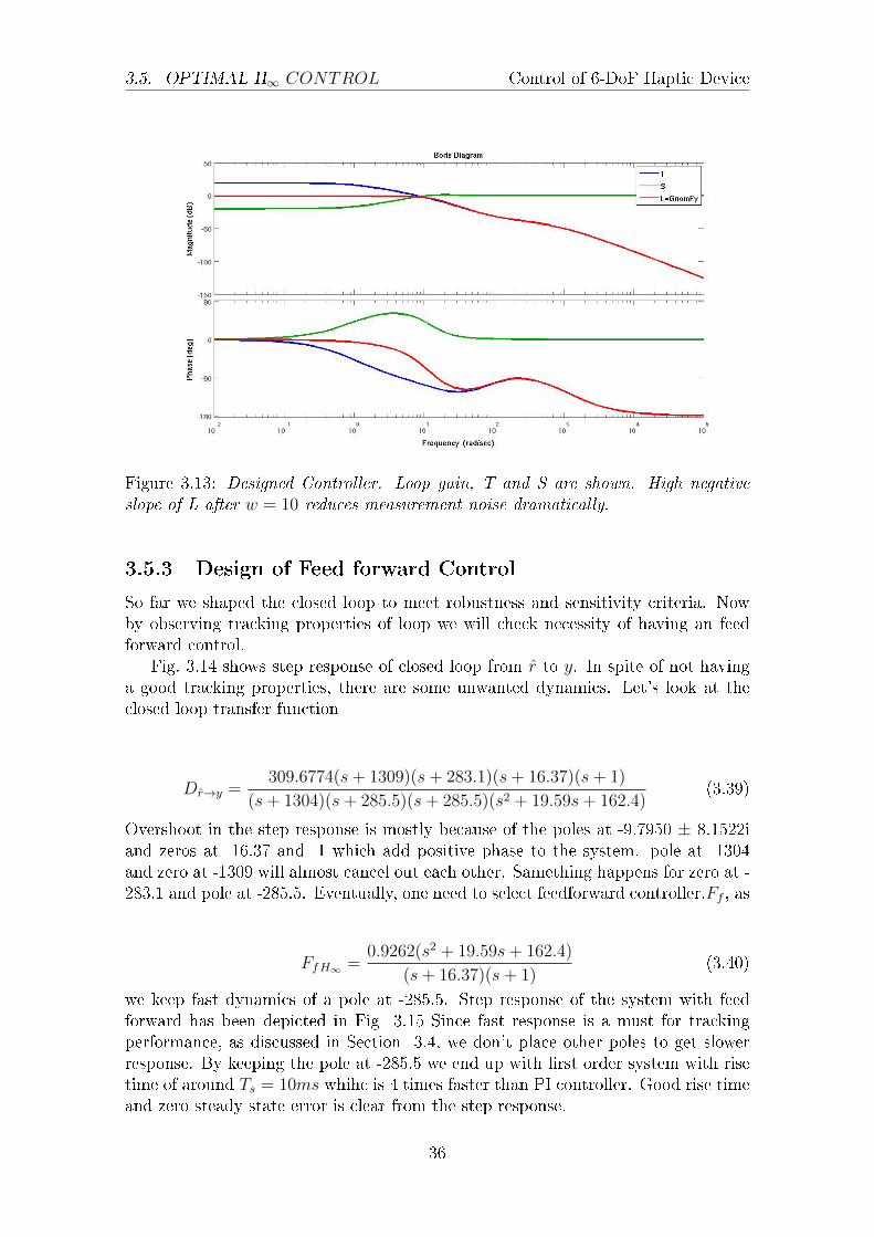
3.5.3 Design of Feed forward Control
So far we shaped the closed loop to meet robustness and sensitivity criteria. Nowby observing tracking properties of loop we will check necessity of having an feedforward control.
Fig. 3.14 shows step response of closed loop from r to y. In spite of not havinga good tracking properties, there are some unwanted dynamics. Let's look at theclosed loop transfer function
Dr→y =309.6774(s+ 1309)(s+ 283.1)(s+ 16.37)(s+ 1)
(s+ 1304)(s+ 285.5)(s+ 285.5)(s2 + 19.59s+ 162.4)(3.39)
Overshoot in the step response is mostly because of the poles at -9.7950 ± 8.1522iand zeros at -16.37 and -1 which add positive phase to the system. pole at -1304and zero at -1309 will almost cancel out each other. Samething happens for zero at -283.1 and pole at -285.5. Eventually, one need to select feedforward controller,Ff , as
FfH∞ =0.9262(s2 + 19.59s+ 162.4)
(s+ 16.37)(s+ 1)(3.40)
we keep fast dynamics of a pole at -285.5. Step response of the system with feedforward has been depicted in Fig 3.15 Since fast response is a must for trackingperformance, as discussed in Section 3.4, we don't place other poles to get slowerresponse. By keeping the pole at -285.5 we end up with rst order system with risetime of around Ts = 10ms whihc is 4 times faster than PI controller. Good rise timeand zero steady state error is clear from the step response.
36
CHAPTER 3. CONTROL DESIGN Control of 6-DoF Haptic Device
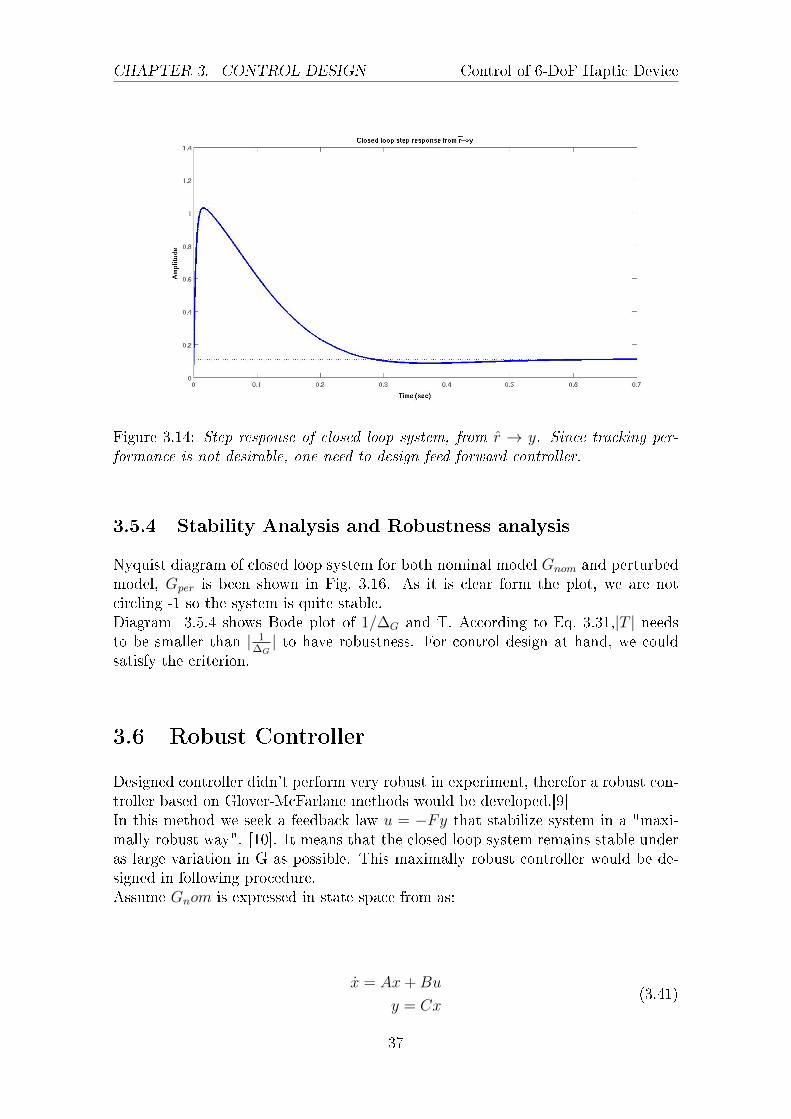
Figure 3.14: Step response of closed loop system, from r → y. Since tracking per-formance is not desirable, one need to design feed forward controller.
3.5.4 Stability Analysis and Robustness analysis
Nyquist diagram of closed loop system for both nominal model Gnom and perturbedmodel, Gper is been shown in Fig. 3.16. As it is clear form the plot, we are notcircling -1 so the system is quite stable.Diagram 3.5.4 shows Bode plot of 1/∆G and T. According to Eq. 3.31,|T | needsto be smaller than | 1
∆G| to have robustness. For control design at hand, we could
satisfy the criterion.
3.6 Robust Controller
Designed controller didn't perform very robust in experiment, therefor a robust con-troller based on Glover-McFarlane methods would be developed.[9]In this method we seek a feedback law u = −Fy that stabilize system in a "maxi-mally robust way". [10]. It means that the closed loop system remains stable underas large variation in G as possible. This maximally robust controller would be de-signed in following procedure.Assume Gnom is expressed in state space from as:
x = Ax+Bu
y = Cx(3.41)
37
3.6. ROBUST CONTROLLER Control of 6-DoF Haptic Device
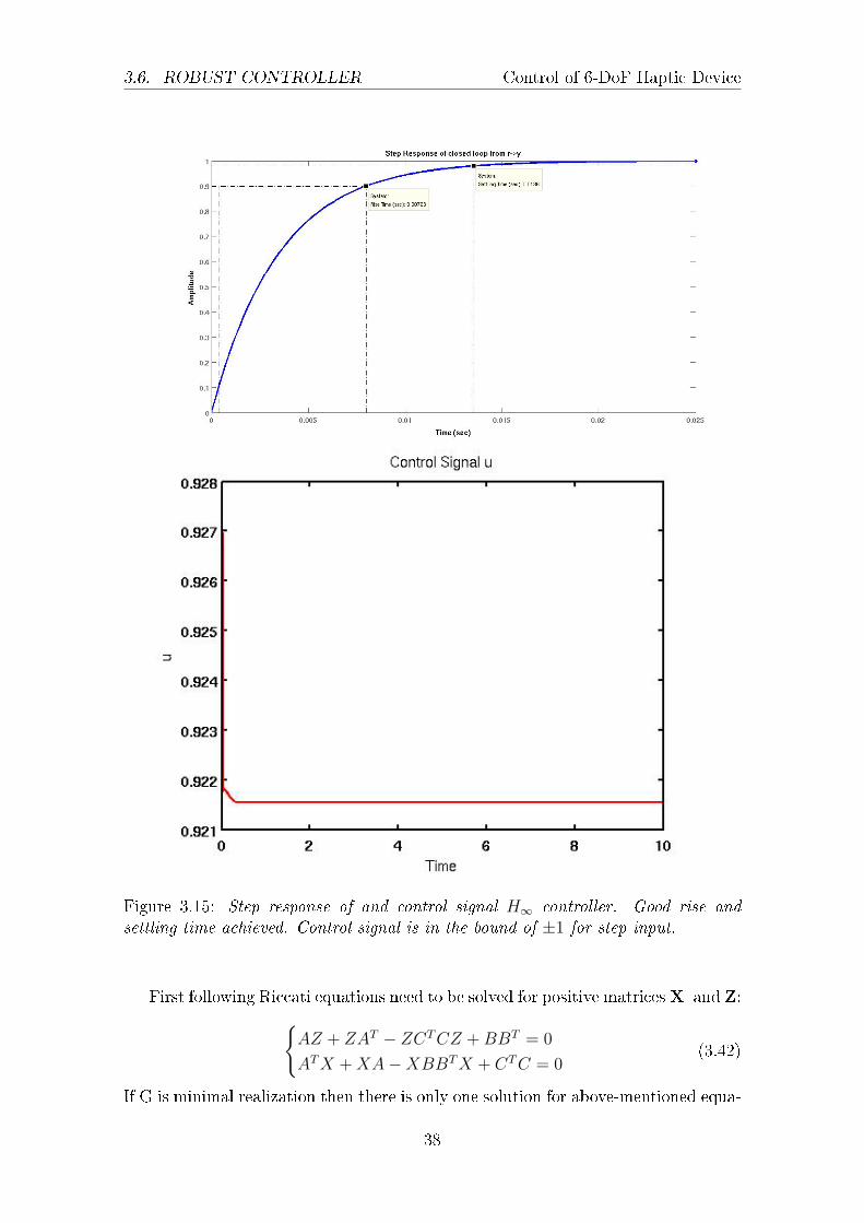
Figure 3.15: Step response of and control signal H∞ controller. Good rise andsettling time achieved. Control signal is in the bound of ±1 for step input.
First following Riccati equations need to be solved for positive matricesX and Z:AZ + ZAT − ZCTCZ +BBT = 0
ATX +XA−XBBTX + CTC = 0(3.42)
If G is minimal realization then there is only one solution for above-mentioned equa-
38
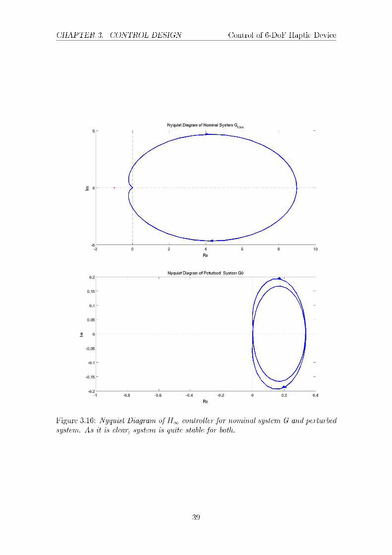
CHAPTER 3. CONTROL DESIGN Control of 6-DoF Haptic Device
Figure 3.16: Nyquist Diagram of H∞ controller for nominal system G and perturbedsystem. As it is clear, system is quite stable for both.
39
3.6. ROBUST CONTROLLER Control of 6-DoF Haptic Device
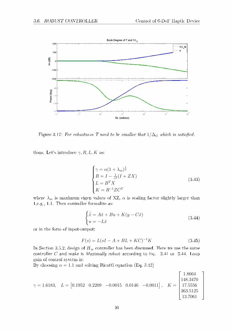
Figure 3.17: For robustness T need to be smaller that 1/∆G which is satised.
tions. Let's introduce γ,R, L,K as:
γ = α(1 + λm)
12
R = I − 1γ2
(I + ZX)
L = BTX
K = R−1ZCT
(3.43)
where λm is maximum eigen values of XZ, α is scaling factor slightly larger than1,e.g., 1.1. Then controller formalize as:
ˆx = Ax+Bu+K(y − Cx)
u = −Lx(3.44)
or in the form of input-output:
F (s) = L(sI − A+BL+KC)−1K (3.45)
In Section 3.5.2, design of H∞ controller has been discussed. Here we use the samecontroller C and make is Maximally robust according to Eq. 3.41 to 3.44. Loopgain of control system is:By choosing α = 1.1 and solving Ricatti equation (Eq. 3.42)
γ = 1.6183, L =[0.1952 0.2209 −0.0015 0.0146 −0.0011
], K =
1.8664
148.347017.5556363.512513.7061
40
CHAPTER 3. CONTROL DESIGN Control of 6-DoF Haptic Device
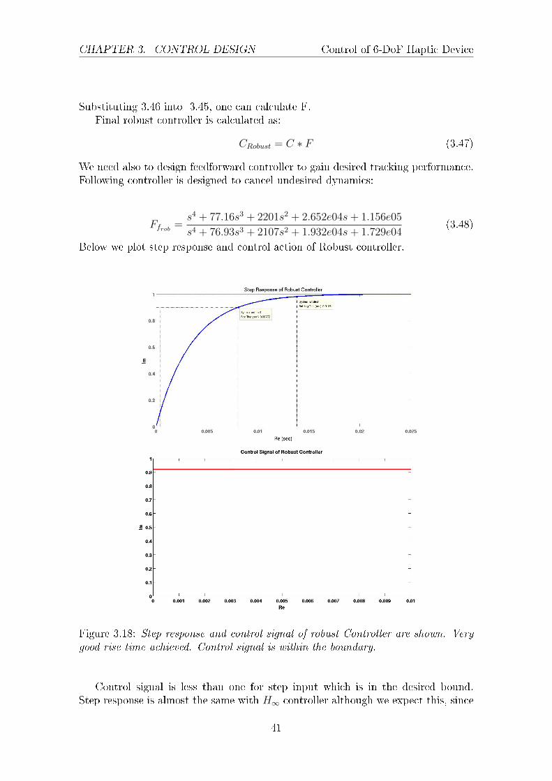
Substituting 3.46 into 3.45, one can calculate F.Final robust controller is calculated as:
CRobust = C ∗ F (3.47)
We need also to design feedforward controller to gain desired tracking performance.Following controller is designed to cancel undesired dynamics:
Ffrob =s4 + 77.16s3 + 2201s2 + 2.652e04s+ 1.156e05
s4 + 76.93s3 + 2107s2 + 1.932e04s+ 1.729e04(3.48)
Below we plot step response and control action of Robust controller.
Figure 3.18: Step response and control signal of robust Controller are shown. Verygood rise time achieved. Control signal is within the boundary.
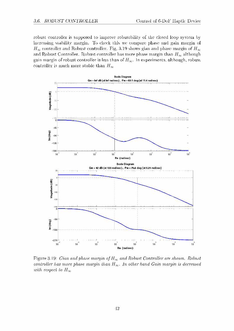
Control signal is less than one for step input which is in the desired bound.Step response is almost the same with H∞ controller although we expect this, since
41
3.6. ROBUST CONTROLLER Control of 6-DoF Haptic Device
robust controller is supposed to improve robustbility of the closed loop system byincreasing stability margin. To check this we compare phase and gain margin ofH∞ controller and Robust controller. Fig. 3.19 shows gian and phase margin of H∞and Robust Controller. Robust controller has more phase margin than H∞ althoughgain margin of robust controller is less than of H∞. In experiments, although, robustcontroller is much more stable than H∞
Figure 3.19: Gian and phase margin of H∞ and Robust Controller are shown. Robustcontroller has more phase margin than H∞. In other hand Gain margin is decreasedwith respect to H∞
42
CHAPTER 3. CONTROL DESIGN Control of 6-DoF Haptic Device
3.7 Robust Controller:Second Method
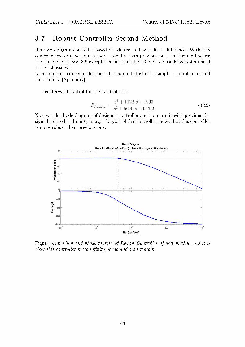
Here we design a controller based on Mclare, but with little dierence. With thiscontroller we achieved much more stability than previous one. In this method weuse same idea of Sec. 3.6 except that instead of F*Gnom, we use F as system needto be robustied.As a result an reduced-order controller computed which is simpler to implement andmore robust.[Appendix]
Feedforward control for this controller is
FfrobNew =s2 + 112.9s+ 1993
s2 + 56.45s+ 943.2(3.49)
Now we plot bode diagram of designed controller and compare it with previous de-signed controller. Innity margin for gain of this controller shows that this controlleris more robust than previous one.
Figure 3.20: Gian and phase margin of Robust Controller of new method. As it isclear this controller more innity phase and gain margin.
43
3.8. PERFORMANCE COMPARISON Control of 6-DoF Haptic Device
3.8 Performance Comparison
Interesting performance of the controllers are stability margins (Gain and Phasemargin), robustibility and tracking performance. Besides, because of very noisymeasurement of current, Torque feedback is very noisy. The controller should at-tenuate measurement noise or if it can't, at least should not amplify that.
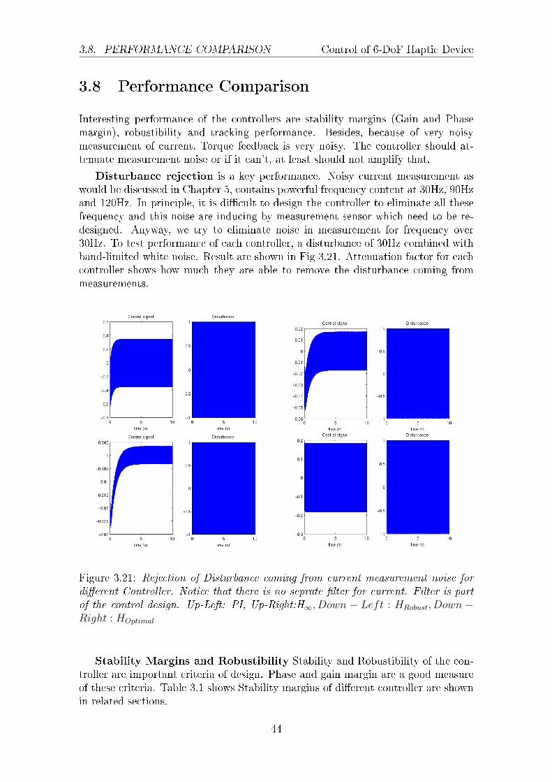
Disturbance rejection is a key performance. Noisy current measurement aswould be discussed in Chapter 5, contains powerful frequency content at 30Hz, 90Hzand 120Hz. In principle, it is dicult to design the controller to eliminate all thesefrequency and this noise are inducing by measurement sensor which need to be re-designed. Anyway, we try to eliminate noise in measurement for frequency over30Hz. To test performance of each controller, a disturbance of 30Hz combined withband-limited white noise. Result are shown in Fig 3.21. Attenuation factor for eachcontroller shows how much they are able to remove the disturbance coming frommeasurements.
Figure 3.21: Rejection of Disturbance coming from current measurement noise fordierent Controller. Notice that there is no seprate lter for current. Filter is partof the control design. Up-Left: PI, Up-Right:H∞, Down − Left : HRobust, Down −Right : HOptimal
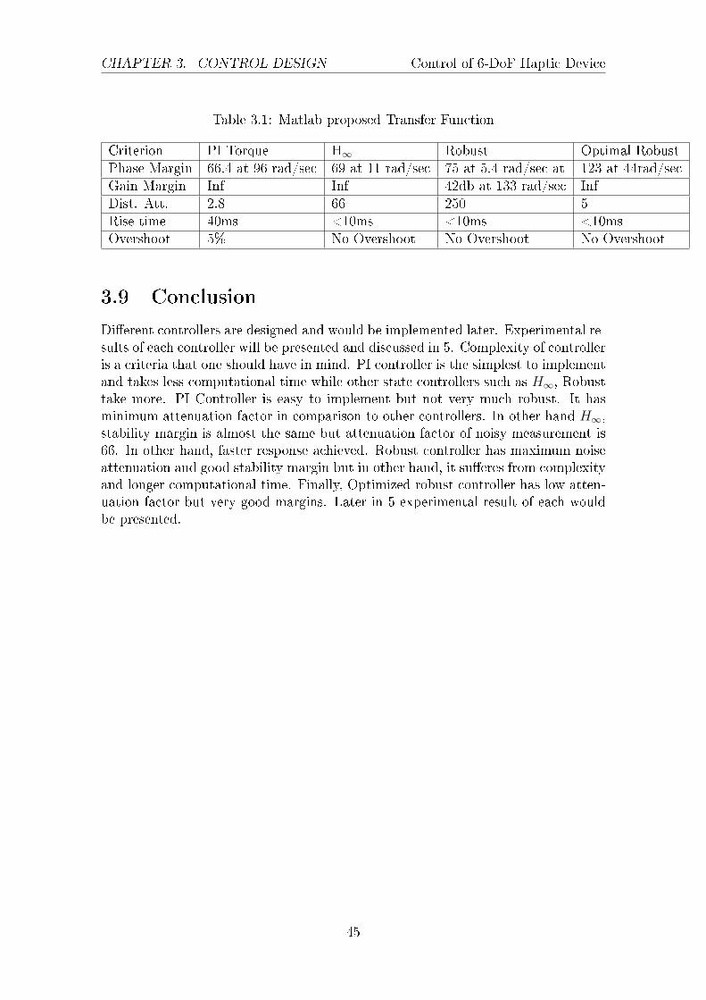
Stability Margins and Robustibility Stability and Robustibility of the con-troller are important criteria of design. Phase and gain margin are a good measureof these criteria. Table 3.1 shows Stability margins of dierent controller are shownin related sections.
44
CHAPTER 3. CONTROL DESIGN Control of 6-DoF Haptic Device
Table 3.1: Matlab proposed Transfer Function
Criterion PI Torque H∞ Robust Optimal RobustPhase Margin 66.4 at 96 rad/sec 69 at 11 rad/sec 75 at 5.4 rad/sec at 123 at 44rad/secGain Margin Inf Inf 42db at 133 rad/sec InfDist. Att. 2.8 66 250 5Rise time 40ms <10ms <10ms <10msOvershoot 5% No Overshoot No Overshoot No Overshoot
3.9 Conclusion
Dierent controllers are designed and would be implemented later. Experimental re-sults of each controller will be presented and discussed in 5. Complexity of controlleris a criteria that one should have in mind. PI controller is the simplest to implementand takes less computational time while other state controllers such as H∞, Robusttake more. PI Controller is easy to implement but not very much robust. It hasminimum attenuation factor in comparison to other controllers. In other hand H∞,stability margin is almost the same but attenuation factor of noisy measurement is66. In other hand, faster response achieved. Robust controller has maximum noiseattenuation and good stability margin but in other hand, it sueres from complexityand longer computational time. Finally, Optimized robust controller has low atten-uation factor but very good margins. Later in 5 experimental result of each wouldbe presented.
45
Chapter 4
Implementation
4.1 Introduction
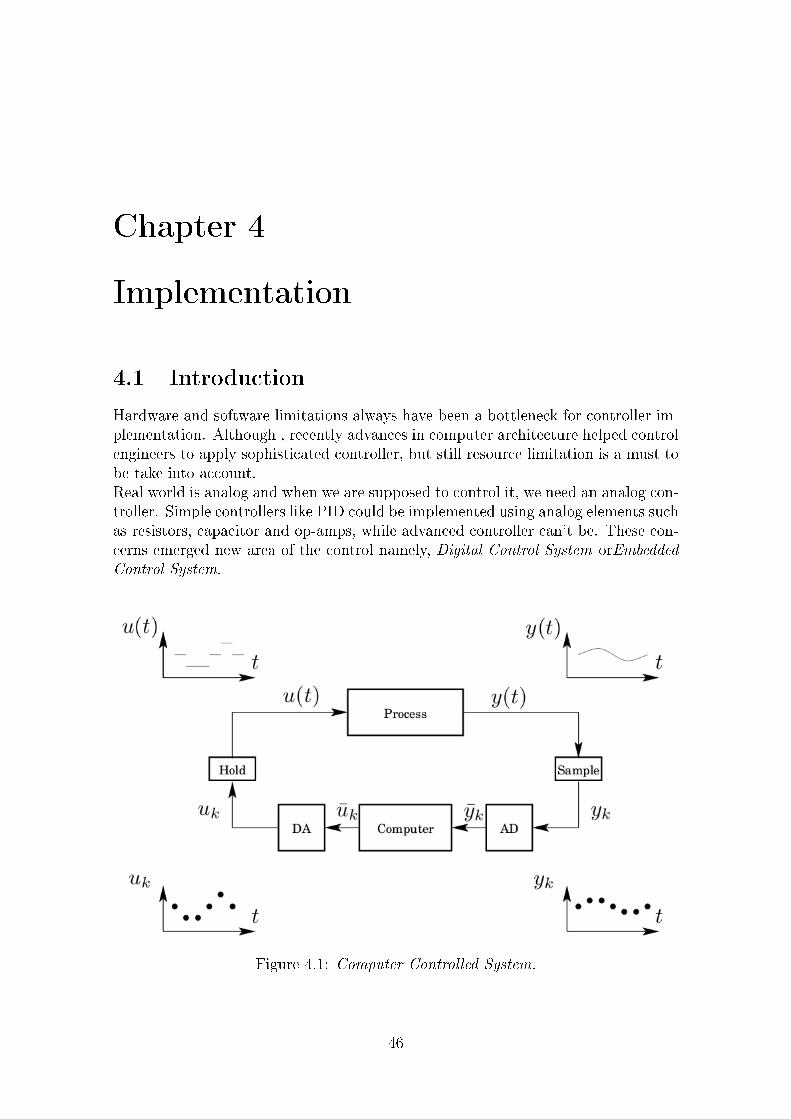
Hardware and software limitations always have been a bottleneck for controller im-plementation. Although , recently advances in computer architecture helped controlengineers to apply sophisticated controller, but still resource limitation is a must tobe take into account.Real world is analog and when we are supposed to control it, we need an analog con-troller. Simple controllers like PID could be implemented using analog elements suchas resistors, capacitor and op-amps, while advanced controller can't be. These con-cerns emerged new area of the control namely, Digital Control System orEmbeddedControl System.
Figure 4.1: Computer Controlled System.
46

CHAPTER 4. IMPLEMENTATION Control of 6-DoF Haptic Device
4.1.1 Design Methods
There are two methods to design the controller. Design inDiscrete or Continuoustime. Following pictures show the concept. One can sample the plant, and then
Figure 4.2: Methods for designing discrete control system. Up:Discrete the plan,design discrete controller, Down: Design analog controller and discrete it.
design discrete controller for it, or just design the controller for the physical plantand then discretize it. Second case is done for this project.
4.2 Discretizing Controller
We have designed continuous time controller for ARES. Here, we will discretize thecontroller to implement it in dSpace. Dierent method are available for discretizingthe controller, to name a few, Forward Dierence(Euler), Backward Dierence andTustin. C(z), discretized controller hold following relation with continuous C(s').
C(z) = C(s′)
where
Forward : s′ =z − 1
Ts
Backward : s′ =z − 1
zTs
Tustin : s′ =2
Ts
z − 1
Ts
(4.1)
We will use Tustin method, since it maps the left hand side of s-plane(stable zerosand poles) to inside of unit circle in discrete space and right hand-side of s-plane tooutside of unit circle.
47
4.2. DISCRETIZING CONTROLLER Control of 6-DoF Haptic Device
4.2.1 Choosing Sampling Time Ts
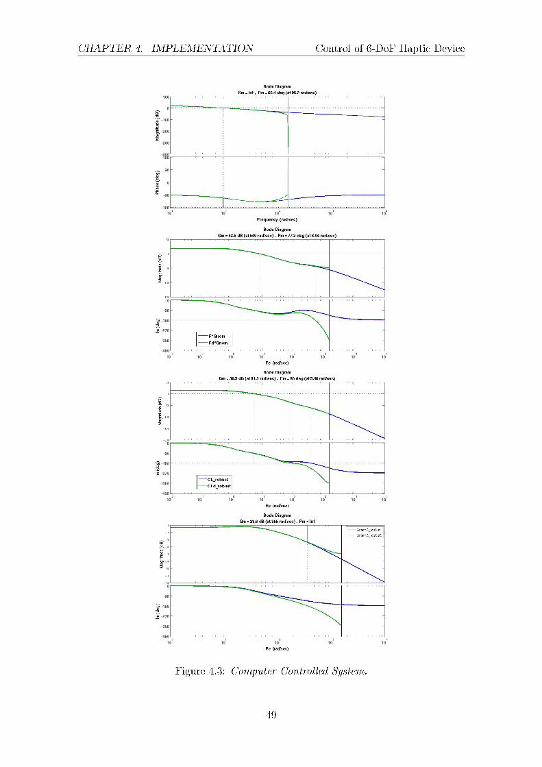
Sampling time can heavily inuence the performance of the controller. So choosingappropriate sampling time is crucial step although there is not so many systematicway for this . It can't be too long to make system unstable and in other hand itshouldn't be too short to increase computational.There is a rule of thumb which built on extensive experiment, but not so muchtheory and that's Ts should b chosen such a way that there will be 4 to 10 samplesper rise time. Ts = 0.002s is a value can satisfy the condition. Although basessimulation one can go to Ts = 0.007s while after that system goes unstable.
Both nominal process and Controllers are discritized with sampling time of Ts =.002 using Tustin method. Following transfer function shows the discritized nominalmodel l, l, l:
Gnom(z) =0.2612z + 0.2612
z − 0.6871(4.2)
Below , bode plot of discretized controllers with Ts = 2ms as shown. As expected,some stability margin are lost because of discritization
48
CHAPTER 4. IMPLEMENTATION Control of 6-DoF Haptic Device
Figure 4.3: Computer Controlled System.
49
4.3. IMPLEMENTATION Control of 6-DoF Haptic Device
4.3 Implementation
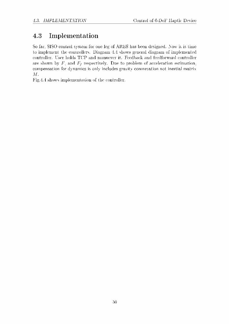
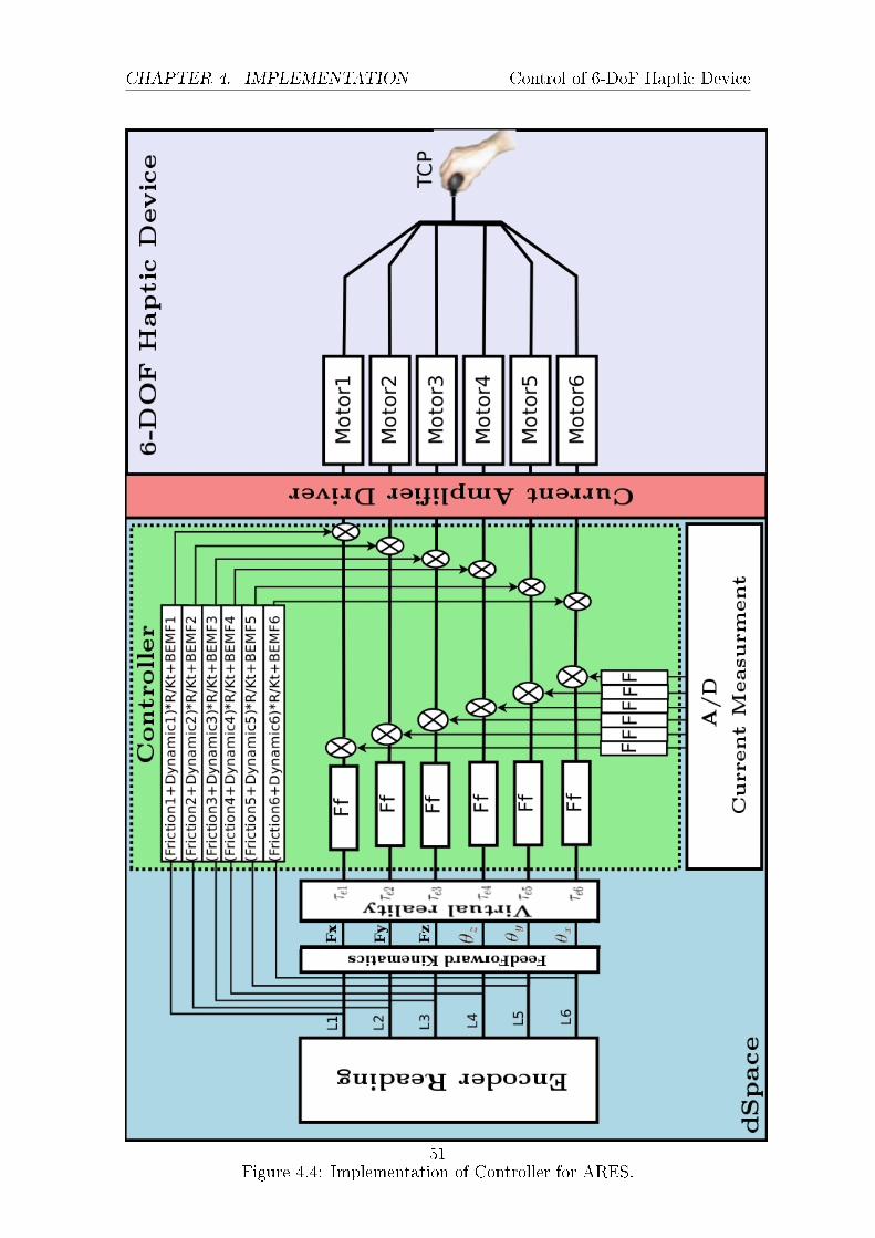
So far, SISO control system for one leg of ARES has been designed. Now it is timeto implement the controllers. Diagram 4.4 shows general diagram of implementedcontroller. User holds TCP and manuever it. Feedback and feedforward controllerare shown by F , and Ff respectively. Due to problem of acceleration estimation,compensation for dynamics is only includes gravity comnesation not inertial matrixM .Fig.4.4 shows implementation of the controller.
50
CHAPTER 4. IMPLEMENTATION Control of 6-DoF Haptic Device
Figure 4.4: Implementation of Controller for ARES.51
Chapter 5
Experiments
5.1 Measurements
5.1.1 Position Measurement
Incremental encoders are coupled to the shaft of the motors and read position data.Output of the encoders are ticks, which can be converted to radian of shaft. Encodersavailable in this project are two phase phase providing both phase A,B. Encodersresolution are 1000 ticks per revolution and dSpace board use two phase reading ofA and B phase of encoder. As result resolution of 2π
4000= 0.00157rad is available for
position measurements which is a good resolution.
5.1.2 Velocity and Acceleration Estimation
Unfortunately there's no direct velocity measurement for ARES. One need to esti-mate velocity from position. What we needed is a time ecient model that does notdepend on the model a lot. So, we decided to use the most trivial way of estimatingthe speed from the position, backward Euler derivative approximation, which is justtaking the dierence of positions divided by the dierence in time. Even thoughthis method amplies the measurement noise via derivation, the computation takesa very short amount of time and the error it introduces is determined to be negligi-ble. Also, we design a low pass lter to remove high frequency measurement noiseand noise coming from discretization. Same approach has been used for accelera-tion estimation. Since acceleration estimation is important for dynamic calculation,derivation of speed for estimation is not a good idea, specially when velocity itselfis estimated based on derivation. Velocity sensor would be benecial for future de-velopment, where one can estimate acceleration using kalman lter. In this thesis,speed has been estimated by taking derivative of position along with a low pass lterwith cut-o frequency of w = 25rad/s. Acceleration has been tried to be estimatedthe same way, although because of very noisy estimation, we could not use it fordynamic compensation for intertia part, M matrix at Eq. 2.6
As shown is Fig. 5.1 Noise in estimation of speed is obvious. Any small vibrationin the shaft would create pulse and each pulse creates 0.00157rad position increment
52
CHAPTER 5. EXPERIMENTS Control of 6-DoF Haptic Device
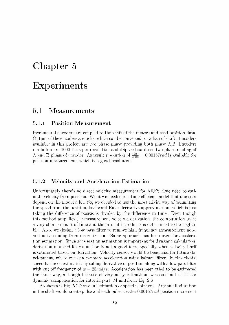
Figure 5.1: Sample signal of position[Rad] and estimated velocity [Rads
]of motor 1.
or decrement. If we select a sampling time of 2ms then we would have a quantizationnoise with amplitude of 0.00157/0.002 = 0.7850rad in estimation. Since we will usespeed estimation later for estimation of acceleration for dynamic compensation, thatwould cause big errors.We tried to use a low pass lter, although that would lter out some high frequencycontent of desired signal and the user will fell that when move the endpoint fast.Adding a tachometer for speed measurement would help to have a better estimationof acceleration which is left for future research.
5.1.3 Current Measurement and analysis
Current measurement is of high importance since it plays main role in the identica-tion and control process. But unfortunately as we discuss later, it is very noisy anddicult to decide how to lter it. Current sensor reads current range of−20A→ 20Aand convert it to the voltage range of −10V → 10V .Then it is read by 16-bits ADCof dSpace. As a result, Available current resolution 20A
216= 6.1035e − 04 which is a
good resolution.Wee need to scale ADC reading to get current signal in [A]. Since it's a linear rela-tion following equation assumed:
I = a ∗ ADC + b; (5.1)
To identify a,b experiments has been done. Table 5.1 shows a and b coecient foreach motor.
Current signal extensively contaminated with noise.(Figure 5.4). Let us to checkfrequency content of the signal to nd which lter suits well.
53
5.1. MEASUREMENTS Control of 6-DoF Haptic Device
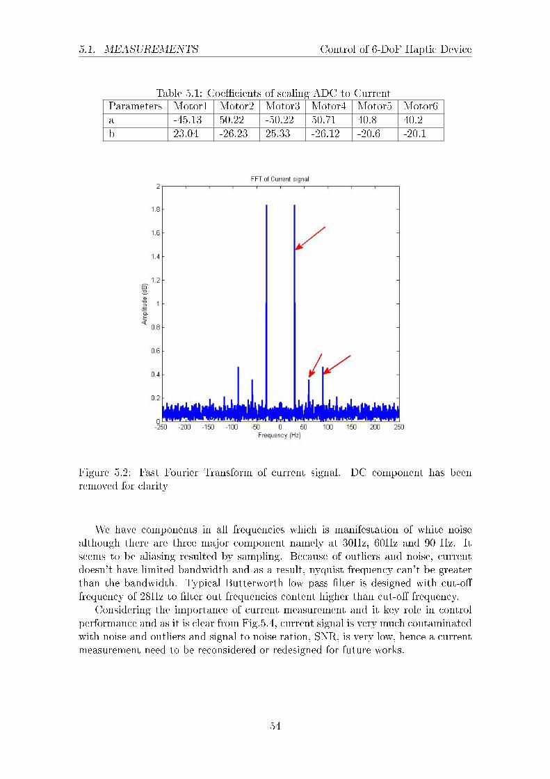
Table 5.1: Coecients of scaling ADC to CurrentParameters Motor1 Motor2 Motor3 Motor4 Motor5 Motor6a -45.13 50.22 -50.22 50.71 40.8 40.2b 23.04 -26.23 25.33 -26.12 -20.6 -20.1
Figure 5.2: Fast Fourier Transform of current signal. DC component has beenremoved for clarity
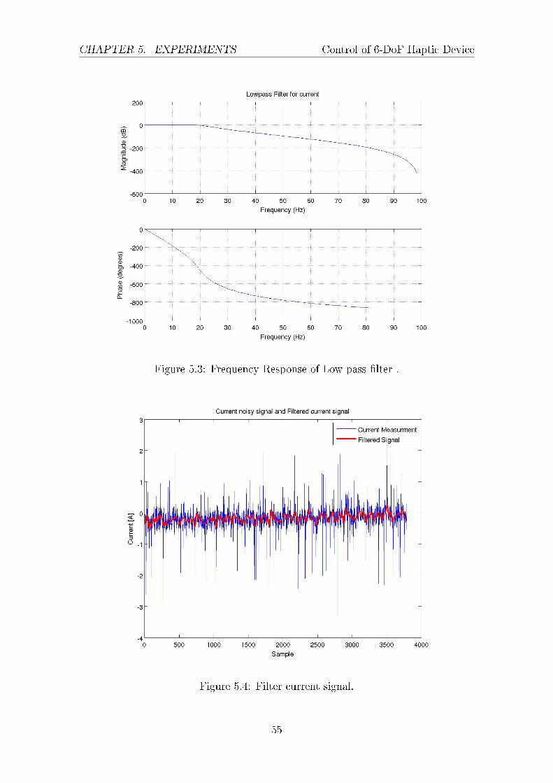
We have components in all frequencies which is manifestation of white noisealthough there are three major component namely at 30Hz, 60Hz and 90 Hz. Itseems to be aliasing resulted by sampling. Because of outliers and noise, currentdoesn't have limited bandwidth and as a result, nyquist frequency can't be greaterthan the bandwidth. Typical Butterworth low pass lter is designed with cut-ofrequency of 28Hz to lter out frequencies content higher than cut-o frequency.
Considering the importance of current measurement and it key role in controlperformance and as it is clear from Fig.5.4, current signal is very much contaminatedwith noise and outliers and signal to noise ration, SNR, is very low, hence a currentmeasurement need to be reconsidered or redesigned for future works.
54
CHAPTER 5. EXPERIMENTS Control of 6-DoF Haptic Device
Figure 5.3: Frequency Response of Low pass lter .
Figure 5.4: Filter current signal.
55
5.2. CONTROLLERS Control of 6-DoF Haptic Device
5.2 Controllers
As discussed in Section 1.1.2, Transparency and Force tracking are the objective ofthe control design. But the question is how to measure these criteria.
For normal control application it is quite convenient to show the performanceof the controller using step responses, while in haptic it is not the case. One of themain objective of the controller was transparent meaning the user should only feelthe dynamic of end-eector or TCP. To show transparency, the force that user feelswhen he/she is moving the TCP needed to be measured. Of course it should beless than a limit to call the device transparent, Less force needed to move the TCP,more transparent the device is.
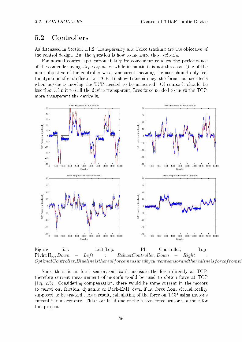
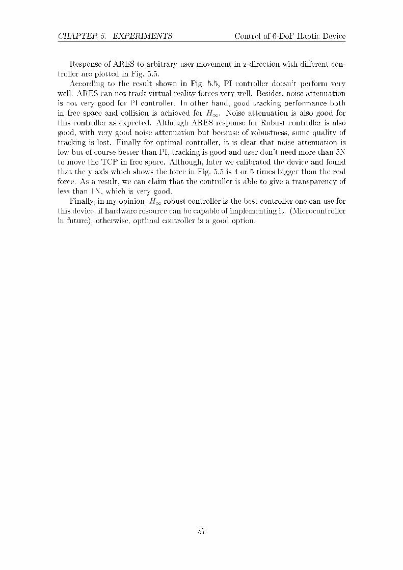
Figure 5.5: Left-Top: PI Controller, Top-Right:H∞, Down − Left : RobustController,Down − Right :OptimalController.Bluelineistherealforcemeasuredbycurrentsensorandtheredlineisforcefromvirtualreality.
Since there is no force sensor, one can't measure the force directly at TCP,therefore current measurement of motor's would be used to obtain force at TCP(Eq. 2.3). Considering compensation, there would be some current in the motorsto cancel out friction, dynamic or Back-EMF even if no force from virtual realitysupposed to be tracked . As a result, calculating of the force on TCP using motor'scurrent is not accurate. This is at least one of the reason force sensor is a must forthis project.
56
CHAPTER 5. EXPERIMENTS Control of 6-DoF Haptic Device
Response of ARES to arbitrary user movement in z-direction with dierent con-troller are plotted in Fig. 5.5.
According to the result shown in Fig. 5.5, PI controller doesn't perform verywell. ARES can not track virtual reality forces very well. Besides, noise attenuationis not very good for PI controller. In other hand, good tracking performance bothin free space and collision is achieved for H∞. Noise attenuation is also good forthis controller as expected. Although ARES response for Robust controller is alsogood, with very good noise attenuation but because of robustness, some quality oftracking is lost. Finally for optimal controller, it is clear that noise attenuation islow but of course better than PI, tracking is good and user don't need more than 5Nto move the TCP in free space. Although, later we calibrated the device and foundthat the y axis which shows the force in Fig. 5.5 is 4 or 5 times bigger than the realforce. As a result, we can claim that the controller is able to give a transparency ofless than 1N, which is very good.
Finally, in my opinion, H∞ robust controller is the best controller one can use forthis device, if hardware resource can be capable of implementing it. (Microcontrollerin future), otherwise, optimal controller is a good option.
57
Chapter 6
Future Work and Conclusion
Haptic Technology is quite novel elds and lots of research group are working on itbut unfortunately there are no much established methods for it. Although, someliterature of robotics may help the reader but still Haptic area is quite dierent.
Control design of haptic is one of the most challenging part of haptic design.Since human is part of the control loop in Haptic, it makes it dicult to design thecontroller. For ARES in other hand, complicated model of the system add complex-ity of control design.Control design of haptic was based on current of motors and in task space, althoughit would be much better to use force sensor at TCP, instead of having current feedback of motors and calculate the force indirectly. Specially in ARES, we had a lotsof problem because of noisy measurement of the current. In spite of attenuatingthe noise from measurements, noise had powerful component in dierent frequencyand it was almost impossible to remove all of them otherwise we would degrade theperformance of the controller and in some cases even make it unstable. It was alimitation of design and either one need to place force sensor for future research orreplace the existing current measurement with a better one.
Adding a taco-meter to measure the speed of the shaft is also useful for futuredevelopment. I believe that, it is crucial for acceleration estimation, since currentlybecause of noisy measurement, acceleration term are very noisy and unusable.
In spite of the problem mentioned, good controllers are designed and imple-mented, although some of them are expensive computationally. Nevertheless, Op-timal robust controller is a good controller in sense of both computation time, ro-bustness and tracking performance.
58
Chapter 7
Appendix
7.1 Controller Implementations
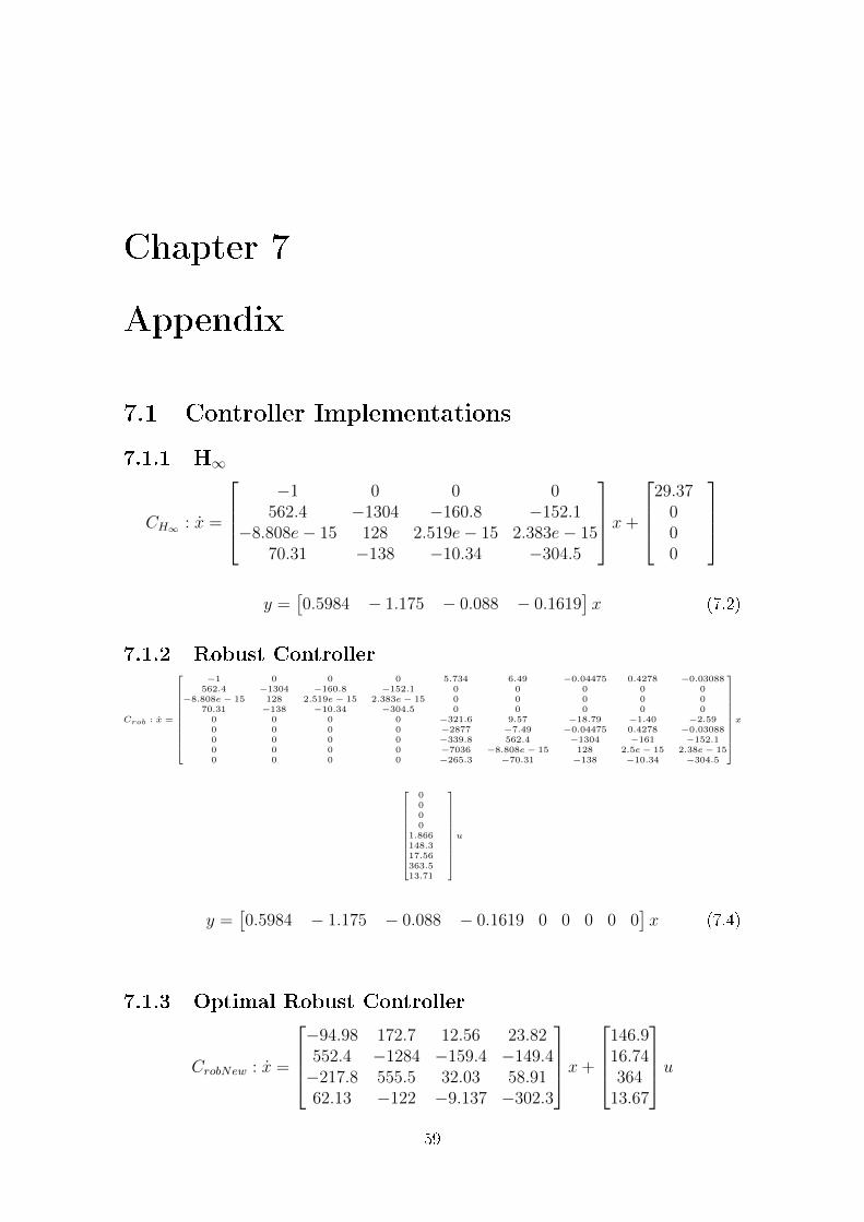
7.1.1 H∞
CH∞ : x =
−1 0 0 0
562.4 −1304 −160.8 −152.1−8.808e− 15 128 2.519e− 15 2.383e− 15
70.31 −138 −10.34 −304.5
x+
29.37
000
y =
[0.5984 − 1.175 − 0.088 − 0.1619
]x (7.2)
7.1.2 Robust Controller
Crob : x =
−1 0 0 0 5.734 6.49 −0.04475 0.4278 −0.03088562.4 −1304 −160.8 −152.1 0 0 0 0 0
−8.808e− 15 128 2.519e− 15 2.383e− 15 0 0 0 0 070.31 −138 −10.34 −304.5 0 0 0 0 0
0 0 0 0 −321.6 9.57 −18.79 −1.40 −2.590 0 0 0 −2877 −7.49 −0.04475 0.4278 −0.030880 0 0 0 −339.8 562.4 −1304 −161 −152.10 0 0 0 −7036 −8.808e− 15 128 2.5e− 15 2.38e− 150 0 0 0 −265.3 −70.31 −138 −10.34 −304.5
x
+
0000
1.866148.317.56363.513.71
u
y =[0.5984 − 1.175 − 0.088 − 0.1619 0 0 0 0 0
]x (7.4)
7.1.3 Optimal Robust Controller
CrobNew : x =
−94.98 172.7 12.56 23.82552.4 −1284 −159.4 −149.4−217.8 555.5 32.03 58.9162.13 −122 −9.137 −302.3
x+
146.916.74364
13.67
u59
7.1. CONTROLLER IMPLEMENTATIONS Control of 6-DoF Haptic Device
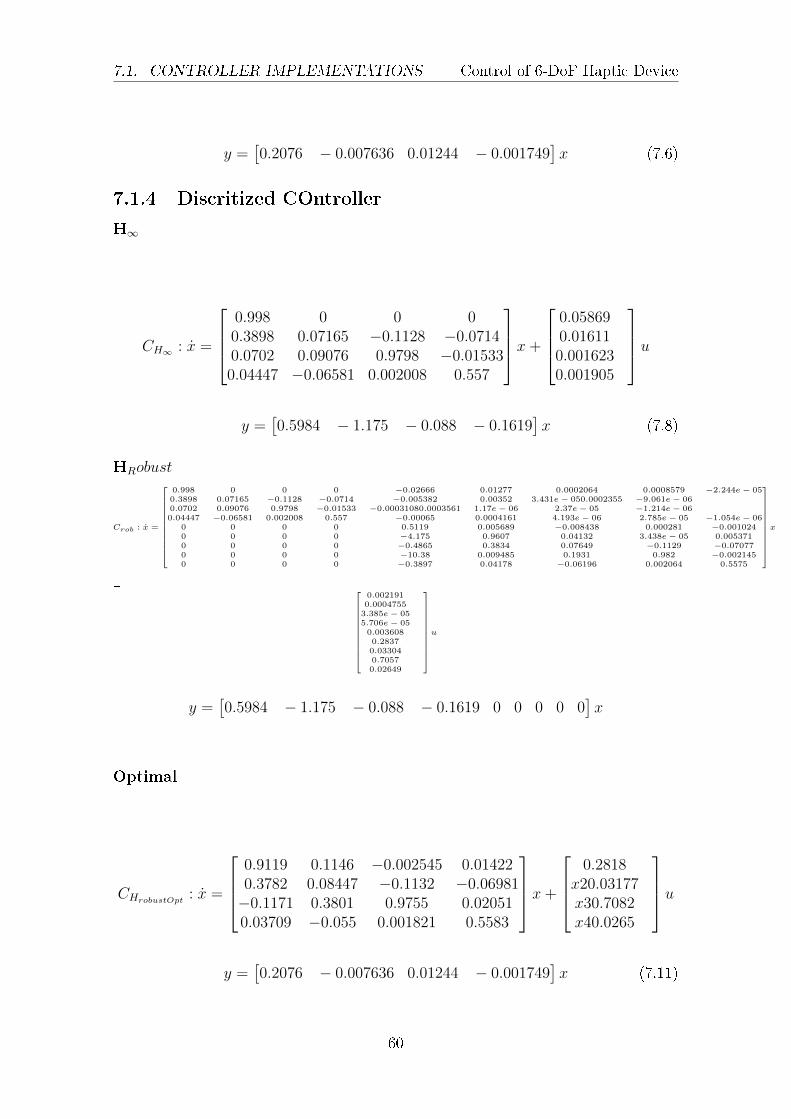
y =[0.2076 − 0.007636 0.01244 − 0.001749
]x (7.6)
7.1.4 Discritized COntroller
H∞
CH∞ : x =
0.998 0 0 00.3898 0.07165 −0.1128 −0.07140.0702 0.09076 0.9798 −0.015330.04447 −0.06581 0.002008 0.557
x+
0.058690.016110.0016230.001905
u
y =[0.5984 − 1.175 − 0.088 − 0.1619
]x (7.8)
HRobust
Crob : x =
0.998 0 0 0 −0.02666 0.01277 0.0002064 0.0008579 −2.244e− 050.3898 0.07165 −0.1128 −0.0714 −0.005382 0.00352 3.431e− 050.0002355 −9.061e− 060.0702 0.09076 0.9798 −0.01533 −0.00031080.0003561 1.17e− 06 2.37e− 05 −1.214e− 060.04447 −0.06581 0.002008 0.557 −0.00065 0.0004161 4.193e− 06 2.785e− 05 −1.054e− 06
0 0 0 0 0.5119 0.005689 −0.008438 0.000281 −0.0010240 0 0 0 −4.175 0.9607 0.04132 3.438e− 05 0.0053710 0 0 0 −0.4865 0.3834 0.07649 −0.1129 −0.070770 0 0 0 −10.38 0.009485 0.1931 0.982 −0.0021450 0 0 0 −0.3897 0.04178 −0.06196 0.002064 0.5575
x
+
0.0021910.00047553.385e− 055.706e− 050.0036080.28370.033040.70570.02649
u
y =[0.5984 − 1.175 − 0.088 − 0.1619 0 0 0 0 0
]x
Optimal
CHrobustOpt : x =
0.9119 0.1146 −0.002545 0.014220.3782 0.08447 −0.1132 −0.06981−0.1171 0.3801 0.9755 0.020510.03709 −0.055 0.001821 0.5583
x+
0.2818
x20.03177x30.7082x40.0265
u
y =[0.2076 − 0.007636 0.01244 − 0.001749
]x (7.11)
60
Bibliography
[1] Gabriel Robles-De-La-Torre. "International Society for Haptics: Haptic tech-nology, an animated explanation". Isfh.org.
[2] Suleman Khan, Control Architecture and design of haptic interfaces, Depart-ment of Machine Design, KTH, Sweden, 2009.
[3] Suleman Khan, Kjell Andersson, Investigation Of Parallel Kinematic Mecha-nism Structure For Haptic Devices, 2nd Nordic Conference on Product LifecycleManagement â NordPLMâ09, Goteborg, January 2009.
[4] Khan Suleman, Andersson K, and Wikander J. âDynamic Based Control Strat-egy for Haptic Devicesâ, Presented at IEEE WorldHaptics International Con-ference, 2011 Turkey.
[5] T. Tjahjowododo, F. Al-Bender, H. Van Brussel Friction Identication andCompesation in a DC Motor , Univertiteit Leuven, Belgium, 2005. 1990.
[6] J. K. Hedrick and A. Girard,Control of Nonlinear Dynamic Systems: Theoryand Applications,2005.
[7] Hanafy M. Omar, Control of Gantry and Tower Cranes, Virginia PolytechnicInstitute and State University, Blacksburg, Virginia, 2003.
[8] Mark W. Spong, M. Vidyasagar Robot Dynamics and Control, John WileySons,Inc, USA, 1989.
[9] Glover, K. McFarlane, D. (1989) "Robust stabilization of normalized coprimefactor plant descriptions with H∞ bounded uncertainty", IEEE Trans. Autom.Control 34,821-830.
[10] Glad, T. and Ljung, L.: Control Theory - Multivariable and Nonlinear methods,Studentlitteratur, 1997.
61