design and optimisation of the architecture and the
TRANSCRIPT

Treball de Fi de Màster
Màster Universitari en Enginyeria Industrial (MUEI)
Design and optimisation of the architecture and
the orientation of utility-scale photovoltaic power plants
REPORT
Author: Eduard Foved Johe Director: Oriol Gomis Bellmunt Call: April 2019
Escola Tècnica Superior d’Enginyeria Industrial de Barcelona


Design and optimisation of the architecture and the orientation of utility-scale photovoltaic power plants Page 1
Abstract
The Spanish and European photovoltaic markets are set for a revival: massive GW
deployments are expected in the coming years. Large utility-scale PV will increasingly take a
role as baseload power plants, displacing dirtier sources of energy. PV project developers will
need to optimise their design practices so as to achieve the most cost-effective solutions
possible.
For all these reasons, the present work is focused on the development of utility-scale PV plants
in the Spanish context.
A MATLAB based programme to simulate PV plants (developed by a former MSc Thesis
student) has been improved and updated with new models, databases and performance
indicators. Three main new models have been added to the original code: tracking system
model, self-shading model and battery model.
The updated MATLAB programme has been used to simulate a 100 MWp PV plant in Seville,
Spain. Several relevant topics have been studied: the selection between string and central
inverters and their DC/AC ratio; the effect of including trackers; the effect of self-shading losses
on land-use; and the inclusion of a battery to provide flat-output response.
Central inverters are found to be still more cost-effective, but string inverters follow the pace.
DC/AC inverter ratios are concluded to be a fundamental designing choice impacting both
performance and cost.
Tracker devices are found to be highly competitive solutions (depending on the location), but
a more careful study on land-use will be required in future works.
A compromise in performance have been found between self-shading losses and land-use:
reducing land-use reduces considerably the energy yield, thus row spacing and module
configuration are fundamental design choices.
Batteries providing services to the grid will play a key role in renewable energy integration,
such as the flat-output response studied. However, further battery cost reductions or
government incentives are required to make these projects more profitable.
The PV industry and policy regulators must work together to ensure a sustainable development
of the European and Spanish utility-scale PV sectors, with PV developers enhancing and
refining their design best practices.

Page 2 Report

Design and optimisation of the architecture and the orientation of utility-scale photovoltaic power plants Page 3
Table of contents
ABSTRACT ___________________________________________________ 1
TABLE OF CONTENTS _________________________________________ 3
LIST OF TABLES ______________________________________________ 7
LIST OF FIGURES _____________________________________________ 9
LIST OF NOMENCLATURES, ABBREVIATIONS AND TERMINOLOGIES 11
1. PREFACE _______________________________________________ 15
1.1. Project origin ................................................................................................. 15
1.2. Motivation ..................................................................................................... 15
1.3. Previous requirements ................................................................................. 15
2. INTRODUCTION __________________________________________ 16
2.1. Objectives ..................................................................................................... 16
2.2. Scope of the project...................................................................................... 16
2.3. Structure ....................................................................................................... 17
3. GENERAL PHOTOVOLTAIC CONTEXT _______________________ 18
3.1. Brief story of photovoltaic energy ................................................................. 18
3.2. The enablers of the photovoltaic success story: cost and efficiency ............ 19
3.2.1. Equipment cost reduction ................................................................................ 20
3.2.2. PV efficiency increase ..................................................................................... 22
3.3. Commercial PV technologies ....................................................................... 23
3.4. The Spanish solar renaissance .................................................................... 24
3.5. Coupling PV installations with batteries ........................................................ 24
4. MATLAB MODEL OF THE PHOTOVOLTAIC PLANT ____________ 26
4.1. General view of the MATLAB model ............................................................ 26
4.2. Tracking system model ................................................................................ 30
4.3. Self-shading model ....................................................................................... 32
4.3.1. Previous calculations of the self-shading model .............................................. 33
4.3.2. Effect on the sky-diffuse and ground-diffuse components of the irradiance .... 35
4.3.2.1. Effect on the sky-diffuse component..................................................... 35
4.3.2.2. Effect on the ground-diffuse component ............................................... 36
4.3.3. Effect on the beam component of the irradiance ............................................. 37
4.3.3.1. Shadow dimensions ............................................................................. 37

Page 4 Report
4.3.3.2. Linear option: reduction of the beam irradiance.................................... 39
4.3.3.3. Non-linear option: self-shading factor reduction of the DC power ......... 39
4.4. Model of the battery ..................................................................................... 41
4.5. Other changes and updates of the PV plant model ..................................... 43
4.5.1. Modification of the incidence angle modifiers (IAM) ......................................... 43
4.5.2. Inclusion of other DC losses ............................................................................ 44
4.5.3. Inclusion of AC losses ...................................................................................... 45
4.5.4. Update of the weather files .............................................................................. 45
4.5.5. Update of the module and the inverter databases ............................................ 45
4.5.6. Inclusion of the performance ratio (PR) calculation .......................................... 45
4.5.7. Modification of the temperature coefficients ..................................................... 46
4.5.8. Modification of the sizing model ....................................................................... 46
5. VALIDATION OF THE NEW MODELS ________________________ 48
5.1. Validation of the tracking model ................................................................... 48
5.2. Validation of the self-shading model ............................................................ 49
6. CASE STUDIES: DEVELOPING A PV UTILITY-SCALE POWER PLANT
IN SEVILLE (SPAIN) _______________________________________ 51
6.1. General assumptions ................................................................................... 51
6.1.1. PV plant location .............................................................................................. 51
6.1.2. PV plant size .................................................................................................... 51
6.1.3. PV modules ..................................................................................................... 51
6.1.4. Inverters ........................................................................................................... 51
6.1.5. LCOE (Levelized Cost of Electricity) ................................................................ 52
6.1.6. PV plant losses ................................................................................................ 53
6.1.7. PV plant layout ................................................................................................. 54
6.2. Case studies development ........................................................................... 55
6.2.1. String vs central inverter architecture under different DC/AC inverter ratios..... 55
6.2.1.1. Specific layout of the different configurations proposed........................ 56
6.2.1.2. Results ................................................................................................. 59
6.2.2. Inclusion of a 1-axis tracking system ................................................................ 61
6.2.2.1. Results ................................................................................................. 61
6.2.3. Self-shading effect on land-use ........................................................................ 65
6.2.3.1. Results ................................................................................................. 66
6.2.4. Inclusion of a battery to provide flat-output ....................................................... 69
6.2.4.1. Results ................................................................................................. 71
6.3. Case studies conclusions ............................................................................ 73

Design and optimisation of the architecture and the orientation of utility-scale photovoltaic power plants Page 5
7. PLANNING AND BUDGET OF THE PROJECT _________________ 74
7.1. Planning of the project .................................................................................. 74
7.2. Budget of the project .................................................................................... 75
8. IMPACTS OF THE PROJECT _______________________________ 76
8.1. Environmental impact ................................................................................... 76
8.1.1. Equivalent and avoided CO2 emissions .......................................................... 76
8.1.2. Land-use ......................................................................................................... 77
8.2. Socioeconomic impacts ................................................................................ 77
CONCLUSIONS ______________________________________________ 78
ACKNOWLEDGMENTS ________________________________________ 79
BIBLIOGRAPHY ______________________________________________ 80
References ............................................................................................................. 80

Page 6 Report
Design and optimisation of the architecture and the orientation of utility-scale photovoltaic power plants Page 7
List of tables
Table 1. PV plant CAPEX divided in its components. ........................................................... 53
Table 2. PV plant OPEX divided in its components. ............................................................. 53
Table 3. PV plant layout depending on the inverter architecture selected. ........................... 54
Table 4. PV plant configurations for a DC/AC inverter ratio of 1. .......................................... 57
Table 5. PV plant configurations for a DC/AC inverter ratio of 1,15. ..................................... 57
Table 6. PV plant configurations for a DC/AC inverter ratio of 1,3. ....................................... 58
Table 7. Summary of the results obtained by the different PV plant configurations (CF-Capacity
Factor, PR-Performance Ratio, LCOE-Levelized Cost of Electricity, Energy Y1-Energy during
year 1). ................................................................................................................................. 59
Table 8. Summary of the results obtained by the PV plant configuration central 2 with and
without tracking system (CF-Capacity Factor, PR-Performance Ratio, LCOE-Levelized Cost
of Electricity, Energy Y1-Energy during year 1). ................................................................... 62
Table 9. General assumptions of the self-shading model ..................................................... 65
Table 10. Summary of the results obtained by the PV plant configuration central 2 with the self-
shading model enabled (CF-Capacity Factor, PR-Performance Ratio, LCOE-Levelized Cost
of Electricity, Energy Y1-Energy during year 1). ................................................................... 66
Table 11. Self-shading losses impact (in percentage) on diffuse (loss on irradiance) and beam
(loss on DC output) components for portrait and landscape configurations. ......................... 67
Table 12. General assumptions for the battery model, with typical efficiency values. ........... 70
Table 13. Summarised results for both cases of flat-output response: 50% and 70% of the PV
plant nominal capacity. ......................................................................................................... 71
Table 14. Budget of the 100 MW PV project in millions of euros (M€) and excluding taxes. 75

Page 8 Report
Design and optimisation of the architecture and the orientation of utility-scale photovoltaic power plants Page 9
List of figures
Figure 1. PV LCOE evolution (2014-2018) for different countries and under different conditions
for yield or considering the tender final price. Source: IEA PVPS [12]. ................................. 19
Figure 2. LCOE comparison between several renewable and conventional energy sources.
Source: BNEF via PV magazine [14]. ................................................................................... 20
Figure 3. PV Price learning curve. Source: Fraunhofer ISE [16]. .......................................... 21
Figure 4. Evolution of lab solar cell efficiency. Source: Fraunhofer ISE [16]. ........................ 22
Figure 5. Schematic representation of the MATLAB model of the photovoltaic plant. Source:
Own ...................................................................................................................................... 26
Figure 6. Representation of the sun position: a) Side view showing the zenith (θz) b) Top view
showing the azimuth (γs). Source [34]. ................................................................................. 27
Figure 7. 1-axis tracking PV plant. Source: PV Magazine [37]. ............................................ 30
Figure 8. Schematic representation of the 1-axis tracking system and its sign convention for
the rotation angle. Source: Own. .......................................................................................... 31
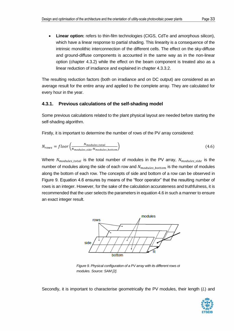
Figure 9. Physical configuration of a PV array with its different rows of modules. Source: SAM
[2]. ........................................................................................................................................ 33
Figure 10. Two possible module configurations: Portrait (left) and landscape (right). Length
and width of the modules are also shown. Source: REC Solar [41] + Own. ......................... 34
Figure 11. Side view of two adjacent rows showing the mask angle. Source: SAM [2]. ....... 35
Figure 12. Shadow dimensions defined by the shadow displacement (g) and the shadow
height (Hs). Source: SAM [2]. ............................................................................................... 37
Figure 13. Schematic representation of the PV power plant with the battery connected in the
AC side. Source: Own. ......................................................................................................... 41
Figure 14. Results comparison for the tracking rotation angle both for SAM and the MATLAB
model. Note that the tracking limit has been set to +-45º. Source: Own. .............................. 48
Figure 15. Results comparison between SAM and the MATLAB code for the self-shading (SS)
model: portraid (a) and landscape (b) module configurations during the 1st of January. Source:

Page 10 Report
Own ...................................................................................................................................... 50
Figure 16. LCOE calculation. Source: Fraunhofer ISE [52]. ................................................. 52
Figure 17. Typical image of a PV plant with string inverters (NOTE: The string inverters seen
in this figure are of lower nominal power than the used in this work). Source: Huawei [50]. . 55
Figure 18. Typical image of a PV plant with central inverters. Source: SMA [51]. ................ 56
Figure 19. DC (blue line) and AC (orange line) output of the PV plant (configuration central 3)
for July 19th, evidencing the occurrence of clipping losses. .................................................. 60
Figure 20. Monthly energy yields for the PV plant with no tracking (blue) and with tracking
(orange). ............................................................................................................................... 63
Figure 21. Comparison between the daily AC output of the PV plant with no tracking (blue) and
with tracking (orange): a) June 21st b) December 21st. ......................................................... 64
Figure 22. Physical configuration of a PV array with its different rows of modules. Source: SAM
[2]. ........................................................................................................................................ 65
Figure 23. Illustration of the power output under shading for portrait (left) and landscape (right)
module configurations. Note that the shade strip produces total shading of the affected cells.
Source: Trina Solar + Own. .................................................................................................. 68
Figure 24. Self-shading DC los against land use for portrait (red) and landscape configuration.
............................................................................................................................................. 69
Figure 25. For the 3rd, 4th and 5th of April: ............................................................................. 72
Figure 26. System power flows during the 4th of April: total system to grid (dashed blue line),
PV to grid (yellow line), PV to battery (charging, red line) and battery to grid (discharging, green
line). ..................................................................................................................................... 73
Figure 27. Gantt chart for the development of a PV plant project in Seville. Source: Own. .. 74

Design and optimisation of the architecture and the orientation of utility-scale photovoltaic power plants Page 11
List of nomenclatures, abbreviations and
terminologies
𝐴𝑚: Module area
AC. Alternating Current
AOI: Angle Of Incidence
a-Si: Amorphous silicon
BNEF: Bloomberg New Energy Finance
BOS: Balance Of the System
CAPEX: Capital Expenditures
CdTe: Cadmium telluride
CIGS: Copper Indium Gallium (Di)Selenide
c-Si: Crystalline silicon
DC: Direct Current
DC/AC ratio: Inverter ratio at nominal capacities of the PV array and the inverter
DHI: Diffuse Horizontal Irradiance
DNI: Direct Normal Irradiance
DOD: Depth of discharge of the battery
𝐸𝑖: component 𝑖 of the POA irradiance
EPC: Engineering, Procurement, Construction
EUR: Euro (€)
E-W: East-West
𝐹𝐹: Fill Factor
𝑔: shadow displacement

Page 12 Report
𝐺𝑖: component 𝑖 of the irradiance
GCR: Ground Coverage Ratio
GHI: Global Horizontal Irradiance
𝐻𝑠: shadow height
IAM: Incidence Angle Modifier
IV curve: curve intensity-current of a photovoltaic module
𝐿: Module height
LCOE: Levelized Cost of Electricity
LID: Light-Induced Degradation
MIP: Minimum Import Price
MLPE: Module Level Power Electronics
MPP: Maximum Power Point
NREL: National Renewable Energy Laboratory
OPEX: Operational Expenditures
PCC: Point of Common Coupling
PERC: Passivated Emitter and Rear Contact
POA: Plane Of Array
PPA: Power Purchase Agreement
PR: Performance Ratio
PV: Photovoltaic
p-type: semiconductor doped with acceptor impurities (boron)
𝑅𝑎𝑠𝑝𝑒𝑐𝑡: Module aspect ratio
SAM: System Advisor Model

Design and optimisation of the architecture and the orientation of utility-scale photovoltaic power plants Page 13
SOC: State of charge of the battery
𝑆𝑆𝐹𝑖: Self-shading loss factor for the component 𝑖 of the irradiance (or in the non-linear case
for the DC output)
STC: Standard Test Conditions (a cell temperature of 25°C and an irradiance of 1000 W/m2
with an air mass 1.5 (AM1.5) spectrum)
USD: US Dollar
𝑊: Module width
Wp: Watt peak

Page 14 Report

Design and optimisation of the architecture and the orientation of utility-scale photovoltaic power plants Page 15
1. Preface
1.1. Project origin
The present project follows the work started by Gabriele Catalano during his Master Thesis
“Development of a model to simulate solar PV plants in MATLAB with a study on the effects
of under-sizing the inverter” (2018) [1], within the research centre CITCEA from the Polytechnic
University of Catalonia (UPC).
This project is intended to upgrade and update the existent models present in Gabriele
Catalano’s MATLAB code, as well as adding new models to enhance the simulation
performance.
1.2. Motivation
The project follows the idea to provide the research centre CITCEA with a MATLAB
programme to simulate photovoltaic plants. Three main reasons arise to justify this motivation:
• Providing a non-expensive (free) PV plants simulator programme;
• Providing a flexible, adaptable and easily tuneable tool to the researchers’ desires;
• Providing an academic tool for students aiming to pursue a professional career in the
renewables and solar sectors.
It is well known the existence of impressive and performant PV plants simulator programmes,
such as PVsyst or SAM (NREL). However, the former is known to be an expensive software
and the latter, while being free, it is not mainly intended to be flexible and modifiable by the
users from a code point of view. Finally, the possibility to interact within the code with the
physical models of the photovoltaic systems could provide students (and future PV
professionals) with a precious understanding on the real behaviour and functioning of PV
plants, which could be of great help in the fast-developing but still young solar industry.
1.3. Previous requirements
Good programming skills within MATLAB environment are required. In addition, a good
understanding of the renewable energy and photovoltaic industry from a techno-economic
point of view is desirable.

Page 16 Report
2. Introduction
2.1. Objectives
The main goal of this project is to continue improving and developing CITCEA’s MATLAB
programme for simulating photovoltaic power plants, a project started by the aforementioned
Gabriele Catalano. The main models added to the programme will be:
• Inclusion of tracking devices;
• A model to consider self-shading losses due to adjacent rows;
• A model to allow the inclusion of batteries.
In addition, several minor changes and updates of the original code will be implemented, such
as updates and expansions of the PV module database, the inverter database and the
meteorological files; or the inclusion of other DC losses not previously considered. These minor
changes are going to be commented in a special chapter in section 4.
Moreover, the resulting upgraded programme is going to be used in several cases studies,
with the aim to analyse and to propose innovative solutions for utility-scale PV plants. The
solutions will be focused on the architecture of the converters (string vs central inverters) and
on the orientation towards the sun (south or E-W orientation, inclusion of trackers, etc.). The
inclusion of batteries to provide grid services will also be studied. The different solutions will
be designed, optimised and assessed considering technical, economic and terrain constraints
criteria.
2.2. Scope of the project
The scope of this project covers the study, implementation and upgrades of a MATLAB
programme to simulate the behaviour of photovoltaic power plants from irradiance to AC
electricity (until the point of common coupling, PCC). Moreover, techno-economic analysis with
financial metrics such as the LCOE (Levelized Cost of Electricity) are also within the scope of
the present project.
On the other hand, the development of a self-shading model is restricted to fixed surfaces with
no tracking. The self-shading model for one-axis tracking is not enabled, since it is required to
develop a new, different and complex model not worth to invest the effort in it (a typical self-
shading model for 1-axis tracking PV systems can be consulted in SAM documentation [2]). It
is important to remark that the tracking model has been developed to assess its
advantages/disadvantages with respect to systems with no tracking, thus simulating both

Design and optimisation of the architecture and the orientation of utility-scale photovoltaic power plants Page 17
systems without self-shading losses will provide a quite accurate comparison.
Regarding the PV technologies studied, a main focus is given to crystalline silicon solar cells.
The programme also allows the selection of thin-film technologies within its database (CdTe,
CIGS and a-Si).
In addition, an extra consideration needs to be given when selecting CdTe modules: both
PVsyst [3] and First Solar [4] (the most important CdTe module manufacturer) suggest that a
spectral correction is required to simulate accurately this technology (especially in high
humidity environments). Nevertheless, since the great majority of PV projects (as well as the
case studies of this project) choose c-Si technologies and given the fact that the error induced
when avoiding these corrections is not remarkable for this project; the development of a model
to correct the spectral irradiance for CdTe technology is out of the scope of this project.
Finally, the simulation of batteries providing services to the grid, the model chosen is restricted
to a flat-output response, a very interesting battery purpose allowing predictable PV outputs.
2.3. Structure
The present work is structured in the following way:
• Firstly, section 3 introduces the reader to photovoltaic energy and its markets, as well
as in the particular case of the Spanish market.
• Secondly, section 4 focuses on explaining the characteristics and particularities of the
existent PV simulation MATLAB programme; and then continues with the explanation
of the new models included (tracking, self-shading and battery models; and the
inclusion or improvement of other submodels).
• Thirdly, section 5 performs a validation of the main models added to the MATLAB code.
• Finally, the improved MATLAB code is used to perform simulations to analyse several
case studies.
In addition, the project also includes several sections at the end with a focus on the planning
of a PV project, a summary of the associated costs and its environmental impacts.
The document ends with a conclusions section stating the main outcomes of this work.

Page 18 Report
3. General photovoltaic context
This section aims to provide the reader with a context on photovoltaic energy, which will
highlight why this thesis is focused on this kind of renewable energy.
Firstly, a first chapter explaining briefly the story of photovoltaic energy is presented (chapter
3.1). This chapter is then followed by the facts that explain the increased importance of PV:
improvements in costs and efficiency (chapter 3.2). A brief explanation of commercial PV
technologies is also included (chapter 3.3). Finally, two extra chapter are included due to
important relevance in the present work: the Spanish solar renaissance (chapter 3.4) and the
coupling of PV installations with batteries (chapter 3.5).
3.1. Brief story of photovoltaic energy
The start point of photovoltaic energy is located in the 19th century: Antoine and Alexandre
Edmond Becquerel discovered the photoelectric effect in 1839 [5], later explained by Albert
Einstein in 1905, who was awarded a Nobel prize for it. Photovoltaic cells use this effect to
generate DC electricity from solar irradiance [6].
However, it is not possible to find a real application for PV cells until the 1960s: electricity
supply for satellites, just when the space race started. Thus, PV cells were seen as a product
for niche markets. In fact, the market being currently dominated by p-type products (mono or
multi crystalline) is also a consequence of the space race: p-type wafers are much more
resistant to the harsh space irradiance and conditions.
Nevertheless, as it happened in many industries before, innovation and cost-performance
improvements brought this niche technology to other markets: from autonomous and remote
applications in need of a reliable energy supply; to the conquest of the whole energy industry,
a process that is in the making.
Recent news state that last year worldwide PV installation topped a new record of 104 GW,
meaning that the current online PV capacity is greater than 500 GW [7]. These numbers take
special relevance when considering the events that occurred in June 2018: the Chinese
government drastically cut off subsidies to solar energy, which in turn produced a stagnation
in Chinese solar deploys (from installing 53 GW in 2017 [8] to 44 GW in 2018 [9]). However,
even if the largest PV market (China) suffered due to changes in subsidy policies, the global
market still increased 2017 PV installations (from 100 GW to the above-mentioned 104 GW).
The reason is simple, cut off in Chinese installations produced an oversupply of PV modules
(since China is also the main player in PV manufacturing). The oversupply led to an abrupt

Design and optimisation of the architecture and the orientation of utility-scale photovoltaic power plants Page 19
drop in prices (up to 34% as stated by Bloomberg New Energy Finance [10]), encouraging
other non-Chinese regions to accelerate their solar deployments. Within these regions, the
European Union was especially favoured by the end of the minimum import price (MIP) on
Chinese PV modules [11], which made prices decrease even more abruptly.
3.2. The enablers of the photovoltaic success story: cost and
efficiency
The explanation of this starting PV success story has its roots in its competitive electricity
production costs. The main indicator for the electricity production costs can be found in the
levelized cost of electricity (LCOE), which is an economic assessment that allows comparing
different power plants or even sources of energy on a comparable basis. In addition, its value
can also be seen as the minimum price at which energy/electricity should be sold in order to
break-even during the lifetime of the project. Its calculation will be explained detail in section
6. Next figure shows the evolution of LCOE for PV installations in different countries:
As it can be observed in Figure 1, PV LCOE has evolved from around 0,1-0,2 EUR/kWh (2014)
to values lower than 0,05 EUR/kWh (2018), which is the same to say that PV has reached
values of LCOE lower than 50 EUR/MWh worldwide. The competitiveness of these values can
be further assessed when compared with the LCOE of other sources of energies: according
Figure 1. PV LCOE evolution (2014-2018) for different countries and under different conditions for yield or considering the
tender final price. Source: IEA PVPS [12].

Page 20 Report
to a report published by Lazard in November 2018 [13], utility-scale PV is already the cheapest
source of electricity in a LCOE basis. A report from Bloomberg New Energy Finance [14] also
reaches the same conclusion, as seen in Figure 2:
These astonishing low costs are led by two major improvements: equipment cost reduction
and efficiency increases of PV technologies.
3.2.1. Equipment cost reduction
The two main components of PV power plants (modules and inverters) have suffered drastic
price drops during the recent years. In fact, as stated by Bloomberg New Energy Finance, the
benchmark CAPEX for a whole utility-scale fixed-axis PV system has decreased from 3,24
USD/Wp in 2010 to less than 1 USD/ Wp in 2018 [15].
Especially remarkable is the decrease in modules cost: current PV modules (2019) can cost
as much as 17% of what they costed back in 2010 (1,85 USD/Wp in 2010 to less than 0,3 USD/
Wp in 2018). What explanation can be given to these data? Two interconnected answers arise:
economies of scale and efficiency improvements.
Economies of scale in the PV industry can be easily summarised with the following graph:
Figure 2. LCOE comparison between several renewable and conventional energy sources. Source: BNEF via PV
magazine [14].

Design and optimisation of the architecture and the orientation of utility-scale photovoltaic power plants Page 21
Figure 3 shows one of the most known graphics within the PV industry: the price learning
curve. The graphic plots the different prices registered on PV technologies (crystalline silicon
or thin-films) as a function of the global cumulative PV capacity at the time the price was
registered. The graphic is plotted on a logarithmic scale.
The higher is the cumulative capacity, the lower is the price, showing perfectly the economies
of scale effect.
But this is not the only conclusion that one can extract from this Figure 3. In fact, the price
learning curve has been used to make really accurate predictions on future PV prices, since
the data trends (shown by the two straight lines in the figure) provide a good estimation tool.
The third conclusion one can come up is the cost reduction potential of thin-films technologies.
Despite not being the popular choice for PV plants (crystalline silicon steals the show), in the
hypothetical case of having the same production capacity as c-Si, thin-films would be largely
the cheapest technologies. The reason for that can be explained by lower raw material
consumption and manufacturing processes that do not include CAPEX and energy intensive
activities such as in c-Si.
However, the cost reduction push cannot be understood without commenting efficiency. A
higher PV efficiency means a higher energy production for the same surface and normally for
the same quantity of raw materials. If this increased energy production compensates the
consequential added costs of increasing efficiency (new manufacturing tools or technologies,
R&D, etc.), the result is a cost reduction on a euro per Watt peak basis (EUR/Wp). In the end,
Figure 3. PV Price learning curve. Source: Fraunhofer ISE [16].

Page 22 Report
a cost dilution is happening, more energy production (or more peak power of PV modules)
dilutes the total costs.
3.2.2. PV efficiency increase
As commented in the previous lines, the efficiency increase is a key enabler in the photovoltaic
success story. Next Figure 4 shows the recent lab efficiency evolution:
As seen in Figure 4, solar cell efficiencies at a lab level have an increasing trend over the last
25 years. However, one could argue that the most popular technology (mono or multi c-Si,
blue lines) have been suffering a stagnation period. Partly this reasoning is true, but only at a
lab scale. It is true that the actual c-Si standard technology (PERC) was developed by
University of New South Wales (UNSW) researchers 30 years ago [17], but the transfer of the
technology to a commercial product has been a tough one. This means that, at a commercial
level, module efficiencies have been increasing intensively during the last decade.
In fact, the c-Si lab cell efficiency record of 26,7% [18] is extremely close to the theoretical
single junction efficiency limit of 29% for crystalline silicon (the Shockley-Queisser limit [19]).
This is why PV researchers are searching for new ways to keep improving efficiency (and
consequently diluting/reducing costs). The latest interest in PV research are tandem devices,
two solar cells stacked together mechanically or electrically that allow overcoming the above-
mentioned efficiency limit. Tandem devices combining silicon solar cells with other materials
(such as perovskite) are on the rise.
Figure 4. Evolution of lab solar cell efficiency. Source: Fraunhofer ISE [16].

Design and optimisation of the architecture and the orientation of utility-scale photovoltaic power plants Page 23
3.3. Commercial PV technologies
This chapter has the objective to present briefly the main PV technologies deployed in PV
projects.
As seen in last Figure 4, numerous PV technologies exist at a lab scale. However, few of them
cross the bridge between research and market, understanding by market the PV projects
market (excluding niche applications such as space exploration, calculators power supply,
solar powered backpacks or small/remote PV applications). In fact, we can currently name
three main technologies in this category:
• Crystalline silicon (c-Si): represents more than a 95% of the PV market [16]. The
technology is based on silicon wafers (monocrystalline or multicrystalline wafers,
depending on the number of silicon crystals), which then are transformed into cells.
During the last year (2018), PERC (Passivated Emitter and Rear Contact)
monocrystalline modules aroused as the dominant and new standard technology [20].
However, other cell technology concepts with higher efficiencies like the IBC
(interdigitated back contact) or the heterojunction solar cells have still their own market
in premium applications [20], with the aim to battle the beginning PERC dominance.
• Cadmium telluride (CdTe): probably the most commercial thin-film technology.
Produced mostly by the American company First Solar [21], the technology seems
ideal for large utility-scale power plants, since it has a superior relative performance in
warm and humid weathers [22].
• Copper Indium Gallium (Di)Selenide (CIGS): always considered as a promising
technology, CIGS has continuously suffered from a poor lab to market transfer (lab and
cell efficiencies are impressive, but module efficiencies are significantly lower due to
cell to module loss). Despite this, the technology is well appreciated in residential
environment due to properties such as the possibility to make flexible modules.
Traditionally, the Japanese manufacturer Solar Frontier dominated CIGS production
[23], but recent Chinese investments such as Hanergy [24] can make an impact on the
technology.
It is possible that some readers miss amorphous silicon (a-Si) in this summary, but the truth is
that the technology that boomed in 2008 is right now obsolete and, in fact, a great number of
a-Si manufacturers are upgrading their lines to other technologies [25].

Page 24 Report
3.4. The Spanish solar renaissance
Since this project’s case studies are going to be focused on the Spanish solar context, this
chapter presents the recent developments in the country concerning photovoltaic energy.
Spain was one of the first countries to bet heavily on solar energy. In fact, the country leaded
the pace at an international level with almost 4,7 GW of capacity installed between 2006 and
2012 [26]. However, the significant effect of the economic crisis together with controversial
decisions made by the Spanish government produced a stagnation in PV installations. Notably,
the retroactive decision to cut already agreed feed-in tariffs decreased Spanish appeal through
investors’ eyes. Some international courts are even starting to rule against the retroactive
decision, meaning that Spain will be forced to pay compensations [27].
Nevertheless, 2018 was a new beginning. The drastic drop in PV module prices together with
a favourable environment to invest in the Spanish solar industry (an optimistic climate and a
new government with “pro-solar” policies). The beginning of the Spanish solar renaissance has
already started: 261,7 MW of new PV systems were installed in Spain during 2018, according
to the Spanish solar energy association (UNEF), meaning that the country has already
surpassed the 5 GW barrier of cumulative capacity [28].
But the best is yet to come: SolarPower Europe, the European solar energy association,
forecasts that Spain will be the hottest European market in 2019, with new PV installations
being able to reach GW scale (SolarPower Europe prospects a medium scenario of new PV
installations of around 9 GW between 2019-2022) [29]. Moreover, this new solar wave is led
by unsubsidised installations both in the form of public tenders (auctions) or private bilateral
power purchase agreements (PPAs) [30] [31].
The awaken of the Spanish solar industry makes very interesting to locate the case studies of
this project in Spain, the European country with the highest annual solar irradiation and now
becoming the PV equivalent for “El Dorado” [32].
3.5. Coupling PV installations with batteries
Being solar PV an intermittent and variable source of electricity, dependent on weather
conditions, the use of storage devices that can help integrating this variable generation takes
an important relevance. Batteries are seen as one of the most promising storage systems
suitable to be coupled to PV installations.
Batteries can provide services to the grid, such as frequency regulation or enhancement of
power quality. They can also provide new business models to PV + battery plants owners,

Design and optimisation of the architecture and the orientation of utility-scale photovoltaic power plants Page 25
since energy arbitrage could become a new source of income. And another possible use is to
provide a more predictable energy output for renewable power plants, for instance, providing
a flat-output for several hours as will be studied in this project.
Regarding battery technologies, it is true that there are many and different ones. However,
lithium-ion batteries have established themselves as the dominant technology, partly because
of the large cost reduction produced by its extensive use and development in the electric
vehicle industry. Other promising battery technologies can arise through innovation, such as
redox flow batteries, which seem ideal for large scale applications if they achieve important
cost reductions [33].
Thus, batteries are expected to become a key player to ensure a good integration of
photovoltaic power plants within the electricity grid. For this reason, a case study of a battery
coupled to the PV plant providing a flat-output service is included in this work.

Page 26 Report
4. MATLAB model of the photovoltaic plant
The purposes of this section are stated in the following lines:
• To present, in a general way, the different parts of the MATLAB model, including the
ones developed by Gabriele Catalano during his MSc Thesis [1];
• To present and explain in detail the new models included in the code during the
development of the present project (tracking, self-shading and battery models);
• To present updates, changes and modifications introduced to the original code (but
not considered as completely new models).
4.1. General view of the MATLAB model
Irradiance models
Position of the sun
Angle of incidence between sun and module
Self-shading model
IV curve / PV module model
Inverter model
Battery model (optional)
GHI/GHI+DHI/DNI+DHI
from weather file
Time and location
Orientation, tracking
enabled?
GCR, physical layout of
the plant
Soiling losses
Other AC losses
Module parameters, Tcell,
number of modules
Inverter parameters,
number of inverters
Battery parameters,
dispatch strategy
Self-shading DC
reduction
Other DC losses
Figure 5. Schematic representation of the MATLAB model of the photovoltaic plant. Source: Own

Design and optimisation of the architecture and the orientation of utility-scale photovoltaic power plants Page 27
Figure 5 presents the general scheme of the PV plant MATLAB model. The scheme shows
the different building blocks corresponding to the physical and technical models included in the
code. Be aware that these building blocks can group different sub-models within them,
particularly when the sub-models are of the same topic and are used to achieve the final goal
of their respective building blocks. In addition, the main external inputs needed for the
completion of the simulations (indicated with the big blue arrows) and several factors for
important losses (written in green and blue colours) are also shown in Figure 5.
Next lines will present the general insights on the MATLAB code. However, more precise
information could be found in Gabriele Catalano’s Master Thesis [1] or in the following chapters
(for the models introduced in the present work).
The MATLAB model starts when introducing the hourly irradiance values for a whole year and
for a specific location (coming from a weather file). The model allows introducing the irradiance
in three different ways depending on its components available in the weather files:
• Global horizontal irradiance (GHI) and diffuse horizontal irradiance (DHI);
• Direct normal irradiance (DNI) and diffuse horizontal irradiance (DHI);
• Global horizontal irradiance (GHI), while estimating the and diffuse horizontal
irradiance (DHI) by means of the Erb’s correlation.
The next step of the model is calculating the sun position at any time for the location desired.
The sun position is defined by the zenith and the azimuth angles (Figure 6). The elevation
angle, the complementary of the zenith, is sometimes preferred in other PV simulation
software.
Given the sun position at any time, the PV module orientation (module azimuth angle and tilt,
Figure 6. Representation of the sun position: a) Side view showing the zenith (θz) b) Top
view showing the azimuth (γs). Source [34].
Page 28 Report
being the latter the module inclination with respect to the horizontal) and the information
whether a 1-axis tracking system is enabled or not; the angle of incidence (AOI) between the
sun and the PV module can be calculated. This magnitude is of utmost importance for the
calculation of the plane of array (POA) irradiance reaching the active PV surfaces. More
precise information about the tracking system model, its implication in the module orientation
and in the same calculations of the AOI will be commented in chapter 4.2.
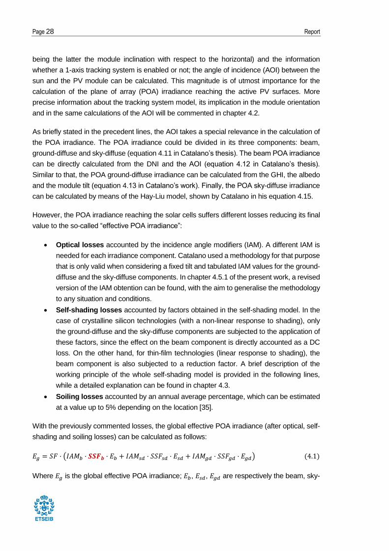
As briefly stated in the precedent lines, the AOI takes a special relevance in the calculation of
the POA irradiance. The POA irradiance could be divided in its three components: beam,
ground-diffuse and sky-diffuse (equation 4.11 in Catalano’s thesis). The beam POA irradiance
can be directly calculated from the DNI and the AOI (equation 4.12 in Catalano’s thesis).
Similar to that, the POA ground-diffuse irradiance can be calculated from the GHI, the albedo
and the module tilt (equation 4.13 in Catalano’s work). Finally, the POA sky-diffuse irradiance
can be calculated by means of the Hay-Liu model, shown by Catalano in his equation 4.15.
However, the POA irradiance reaching the solar cells suffers different losses reducing its final
value to the so-called “effective POA irradiance”:
• Optical losses accounted by the incidence angle modifiers (IAM). A different IAM is
needed for each irradiance component. Catalano used a methodology for that purpose
that is only valid when considering a fixed tilt and tabulated IAM values for the ground-
diffuse and the sky-diffuse components. In chapter 4.5.1 of the present work, a revised
version of the IAM obtention can be found, with the aim to generalise the methodology
to any situation and conditions.
• Self-shading losses accounted by factors obtained in the self-shading model. In the
case of crystalline silicon technologies (with a non-linear response to shading), only
the ground-diffuse and the sky-diffuse components are subjected to the application of
these factors, since the effect on the beam component is directly accounted as a DC
loss. On the other hand, for thin-film technologies (linear response to shading), the
beam component is also subjected to a reduction factor. A brief description of the
working principle of the whole self-shading model is provided in the following lines,
while a detailed explanation can be found in chapter 4.3.
• Soiling losses accounted by an annual average percentage, which can be estimated
at a value up to 5% depending on the location [35].
With the previously commented losses, the global effective POA irradiance (after optical, self-
shading and soiling losses) can be calculated as follows:
𝐸𝑔 = 𝑆𝐹 · (𝐼𝐴𝑀𝑏 · 𝑺𝑺𝑭𝒃 · 𝐸𝑏 + 𝐼𝐴𝑀𝑠𝑑 · 𝑆𝑆𝐹𝑠𝑑 · 𝐸𝑠𝑑 + 𝐼𝐴𝑀𝑔𝑑 · 𝑆𝑆𝐹𝑔𝑑 · 𝐸𝑔𝑑) (4.1)
Where 𝐸𝑔 is the global effective POA irradiance; 𝐸𝑏, 𝐸𝑠𝑑, 𝐸𝑔𝑑 are respectively the beam, sky-

Design and optimisation of the architecture and the orientation of utility-scale photovoltaic power plants Page 29
diffuse and ground-diffuse POA irradiances; 𝑆𝐹 is the soiling factor (obtained as the
complementary fraction of the soiling losses); 𝐼𝐴𝑀𝑏, 𝐼𝐴𝑀𝑠𝑑, 𝐼𝐴𝑀𝑔𝑑 are the incidence angle
modifiers for their respective irradiance components; and 𝑆𝑆𝐹𝑏, 𝑆𝑆𝐹𝑠𝑑, 𝑆𝑆𝐹𝑔𝑑 are the self-
shading factors for the beam, sky-diffuse and ground-diffuse components of the irradiance. It
is important to notice that 𝑆𝑆𝐹𝑏 is highlighted in red, indicating that it is only considered when
using thin-film technologies.
The self-shading model, briefly commented before, requires as external inputs the ground
coverage ratio (GCR, fraction of area occupied by PV modules to the total area) and the
physical layout of the plant (meaning the number of modules along the side and along the
bottom of a row; and the total number of modules to compute the number of rows). As results,
the self-shading factors to reduce beam (thin-film case), sky-diffuse and ground-diffuse
components of the irradiance are obtained (𝑆𝑆𝐹𝑏, 𝑆𝑆𝐹𝑠𝑑, 𝑆𝑆𝐹𝑔𝑑), as well as a photovoltaic DC
output loss factor (𝑆𝑆𝐹𝐷𝐶) to account for the effect on the beam component when using
crystalline silicon technologies. This model is extensively explained in chapter 4.3 and it is
based on the model proposed by SAM (System Advisor Model) developers [2].
The IV curve/PV module model computes first the IV curve at reference/standard test
conditions with the information coming from the module parameters. Once obtained, the
reference IV curve is modified to the particular cell temperature and irradiation conditions at
any time, thanks to temperature coefficients for current and voltage (presents in the module
parameters) and to the proportional effect on some parameters of the change in irradiance.
Then, the maximum power point (MPP) can be computed at any conditions during the whole
year and, given the number of modules and its electrical configuration (modules in series per
string and number of strings), the power, current and voltages of the array can be obtained. A
more detailed explanation of this methodology and of the different sub-models (such as the
model to obtain the cell temperature) can be found in section 4.6 of Catalano’s Thesis.
The DC output of the PV array is reduced as a consequence of computing differing DC losses.
Firstly, DC cabling losses are accounted thanks to a simple model that estimates the
equivalent resistance of the DC wirings (section 4.10.1 of Catalano’s work). Secondly, several
other DC losses are accounted as reduction factors of the resulting DC power. Within this
group of losses, the self-shading factor reduction of the DC power (𝑆𝑆𝐹𝐷𝐶) can be included.
Other losses factors such as the module mismatch or the diodes connections are also
considered. A more detailed and complete explanation of these losses and their computation
within the code can be found in chapter 4.5.2 of the present work.
The DC output is transformed to AC thanks to the inverter model. For this purpose, the Sandia
inverter model [36] is selected, as commented by Catalano in chapter 4.9 of his work. This
model is based on experimental data and is the same one used by SAM. The model needs

Page 30 Report
the external input of several inverter parameters, which include the operation limits in terms of
power, current and voltage as well as the experimental coefficients used by the Sandia model.
This AC output is then reduced as a consequence of computing the AC cabling losses,
accounted as a reduction factor of the AC power. Transformer losses are considered out of
the scope of the project but can easily be implemented in the same manner as AC cabling
losses. A more detailed explanation of these losses can be found in chapter 4.5.3.
Finally, an optional battery model has been implemented during the development of this thesis.
The model needs the input of different battery parameters as well as the dispatch strategy or
mode of operation. For the sake of the simulation, the mode of operation has been set to
providing a flat-output response, a service to the grid of great interest due to reducing the
variability of the PV plant output. A detailed explanation of this model and of the dispatch
strategy can be found in chapter 4.4.
4.2. Tracking system model
The tracking model implemented corresponds to the so-called 1-axis tracking (or single axis).
In this tracking configuration, the rows of PV modules rotate about a horizontal axis orientated
north-south, allowing the modules to follow the sun path (from east in the morning to west in
the evening). Figure 7 shows the typical configuration of 1-axis tracking PV plants.
Figure 7 picture is taken facing the south, thus in this moment PV modules are facing east
(modules facing the left part of the picture). The system will follow the sun movement along
the day, ending with a west orientation during the evening (modules facing the right part of the
picture).
Other tracking systems, such as azimuth axis tracking, 1-axis tracking with tilted rotation axis
or 2-axis tracking are out of the scope of this model. Two convergent reasons exist to make
Figure 7. 1-axis tracking PV plant. Source: PV Magazine [37].
Rotation axis
S
W
N
E

Design and optimisation of the architecture and the orientation of utility-scale photovoltaic power plants Page 31
this exclusion decision: none of the omitted tracking systems are seen as cost-effective
solutions by experts (suggested by BNEF [38]) and the exclusion of them also simplifies the
model formulation.
The proposed model is based on the work of Marion and Dobos in their work “Rotation Angle
for the Optimum Tracking of One-Axis Trackers” [39]. This is the reference document used by
SAM in its tracking implementation. However, the document describes a set of generalised
equations allowing tilted 1-axis tracking. For this reason, the present project has simplified
these equations to 1-axis horizontal tracking:
|𝜎| = 𝑎𝑏𝑠(tan−1(tan𝑍 · sin(𝛾𝑠 − 𝛾𝑎𝑥𝑖𝑠))) (4.2)
Where |𝜎| is the absolute value of the 1-axis tracker rotation angle, 𝑍 is the sun zenith, 𝛾𝑠 is
the sun azimuth and 𝛾𝑎𝑥𝑖𝑠 is the azimuth angle of the rotation axis. As previously discussed,
the tracking device modelled has a rotation axis orientated north-south, that in the sun angles
convention taken in the MATLAB code means 𝛾𝑎𝑥𝑖𝑠 = 0° (or analogously, 𝛾𝑎𝑥𝑖𝑠 = 180°).
A convention to decide the sign of the rotation angle 𝜎 is taken to define completely the tracking
system:
{
𝜎 = 0 𝑚𝑒𝑎𝑛𝑠 𝑚𝑜𝑑𝑢𝑙𝑒𝑠 ℎ𝑜𝑟𝑖𝑧𝑜𝑛𝑡𝑎𝑙 𝜎 > 0 𝑚𝑒𝑎𝑛𝑠 𝑚𝑜𝑑𝑢𝑙𝑒𝑠 𝑓𝑎𝑐𝑖𝑛𝑔 𝑒𝑎𝑠𝑡 𝜎 < 0 𝑚𝑒𝑎𝑛𝑠 𝑚𝑜𝑑𝑢𝑙𝑒𝑠 𝑓𝑎𝑐𝑖𝑛𝑔 𝑤𝑒𝑠𝑡
(4.3)
In order to define the previous convention, the following equation is proposed to calculate the
ideal rotation angle:
𝜎𝑖𝑑𝑒𝑎𝑙 = −𝑠𝑖𝑔𝑛(𝛾𝑠) · |𝜎| (4.4)
Equation 4.4 takes the sign of the sun azimuth as an indicator to set the sign for the rotation
angle. Since the sun azimuth is negative for east positions and positive for west positions (in
our MATLAB notation), a negative sign is added in equation 4.4. This convention is shown in
Figure 8.
East West
𝜎 = 0 𝜎 > 0 𝜎 < 0
Figure 8. Schematic representation of the 1-axis tracking system and its sign convention for the rotation angle. Source:
Own.
Page 32 Report
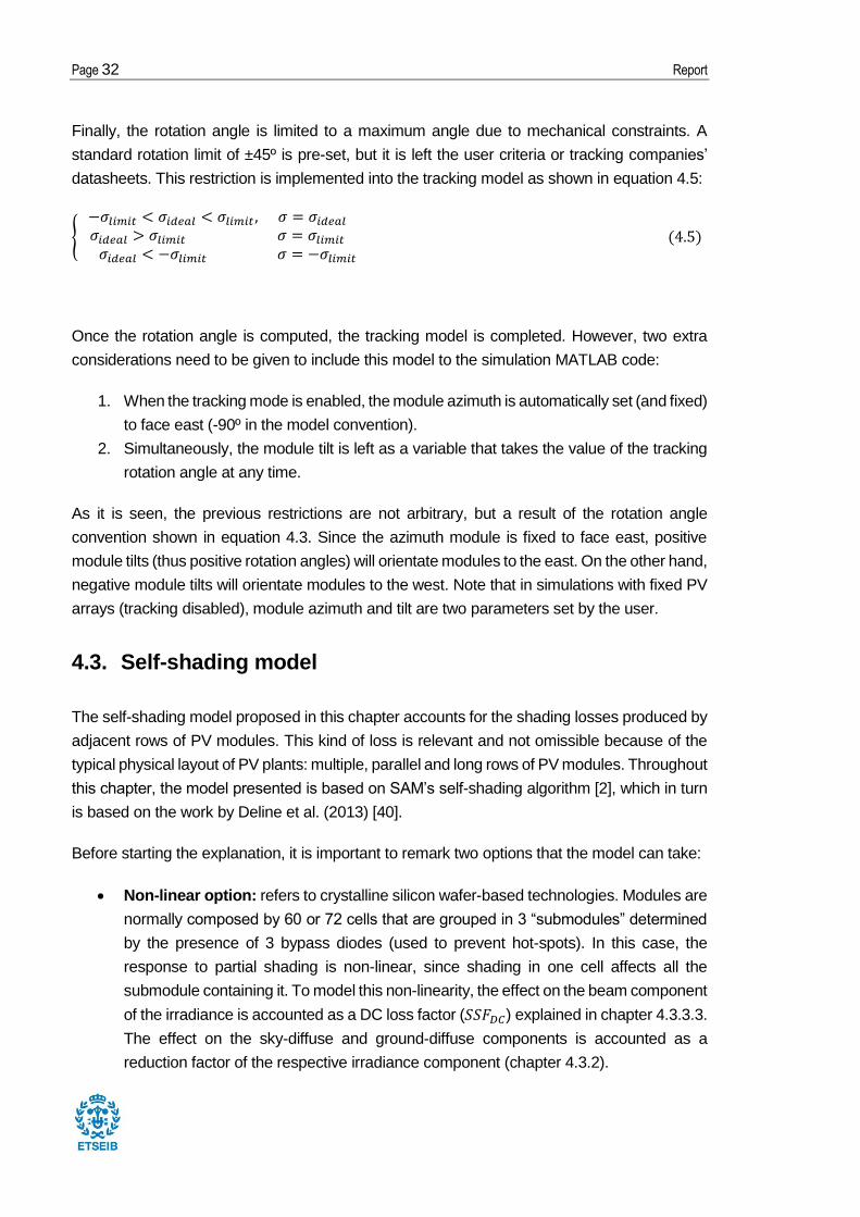
Finally, the rotation angle is limited to a maximum angle due to mechanical constraints. A
standard rotation limit of ±45º is pre-set, but it is left the user criteria or tracking companies’
datasheets. This restriction is implemented into the tracking model as shown in equation 4.5:
{
−𝜎𝑙𝑖𝑚𝑖𝑡 < 𝜎𝑖𝑑𝑒𝑎𝑙 < 𝜎𝑙𝑖𝑚𝑖𝑡 , 𝜎 = 𝜎𝑖𝑑𝑒𝑎𝑙𝜎𝑖𝑑𝑒𝑎𝑙 > 𝜎𝑙𝑖𝑚𝑖𝑡 𝜎 = 𝜎𝑙𝑖𝑚𝑖𝑡
𝜎𝑖𝑑𝑒𝑎𝑙 < −𝜎𝑙𝑖𝑚𝑖𝑡 𝜎 = −𝜎𝑙𝑖𝑚𝑖𝑡
(4.5)
Once the rotation angle is computed, the tracking model is completed. However, two extra
considerations need to be given to include this model to the simulation MATLAB code:
1. When the tracking mode is enabled, the module azimuth is automatically set (and fixed)
to face east (-90º in the model convention).
2. Simultaneously, the module tilt is left as a variable that takes the value of the tracking
rotation angle at any time.
As it is seen, the previous restrictions are not arbitrary, but a result of the rotation angle
convention shown in equation 4.3. Since the azimuth module is fixed to face east, positive
module tilts (thus positive rotation angles) will orientate modules to the east. On the other hand,
negative module tilts will orientate modules to the west. Note that in simulations with fixed PV
arrays (tracking disabled), module azimuth and tilt are two parameters set by the user.
4.3. Self-shading model
The self-shading model proposed in this chapter accounts for the shading losses produced by
adjacent rows of PV modules. This kind of loss is relevant and not omissible because of the
typical physical layout of PV plants: multiple, parallel and long rows of PV modules. Throughout
this chapter, the model presented is based on SAM’s self-shading algorithm [2], which in turn
is based on the work by Deline et al. (2013) [40].
Before starting the explanation, it is important to remark two options that the model can take:
• Non-linear option: refers to crystalline silicon wafer-based technologies. Modules are
normally composed by 60 or 72 cells that are grouped in 3 “submodules” determined
by the presence of 3 bypass diodes (used to prevent hot-spots). In this case, the
response to partial shading is non-linear, since shading in one cell affects all the
submodule containing it. To model this non-linearity, the effect on the beam component
of the irradiance is accounted as a DC loss factor (𝑆𝑆𝐹𝐷𝐶) explained in chapter 4.3.3.3.
The effect on the sky-diffuse and ground-diffuse components is accounted as a
reduction factor of the respective irradiance component (chapter 4.3.2).
Design and optimisation of the architecture and the orientation of utility-scale photovoltaic power plants Page 33
• Linear option: refers to thin-film technologies (CIGS, CdTe and amorphous silicon),
which have a linear response to partial shading. This linearity is a consequence of the
intrinsic monolithic interconnection of the different cells. The effect on the sky-diffuse
and ground-diffuse components is accounted in the same way as in the non-linear
option (chapter 4.3.2) while the effect on the beam component is treated also as a
linear reduction of irradiance and explained in chapter 4.3.3.2.
The resulting reduction factors (both on irradiance and on DC output) are considered as an
average result for the entire array and applied to the complete array. They are calculated for
every hour in the year.
4.3.1. Previous calculations of the self-shading model
Some previous calculations related to the plant physical layout are needed before starting the
self-shading algorithm.
Firstly, it is important to determine the number of rows of the PV array considered:
𝑁𝑟𝑜𝑤𝑠 = 𝑓𝑙𝑜𝑜𝑟 (𝑁𝑚𝑜𝑑𝑢𝑙𝑒𝑠_𝑡𝑜𝑡𝑎𝑙
𝑁𝑚𝑜𝑑𝑢𝑙𝑒𝑠_𝑠𝑖𝑑𝑒·𝑁𝑚𝑜𝑑𝑢𝑙𝑒𝑠_𝑏𝑜𝑡𝑡𝑜𝑚) (4.6)
Where 𝑁𝑚𝑜𝑑𝑢𝑙𝑒𝑠_𝑡𝑜𝑡𝑎𝑙 is the total number of modules in the PV array, 𝑁𝑚𝑜𝑑𝑢𝑙𝑒𝑠_𝑠𝑖𝑑𝑒 is the
number of modules along the side of each row and 𝑁𝑚𝑜𝑑𝑢𝑙𝑒𝑠_𝑏𝑜𝑡𝑡𝑜𝑚 is the number of modules
along the bottom of each row. The concepts of side and bottom of a row can be observed in
Figure 9. Equation 4.6 ensures by means of the “floor operator” that the resulting number of
rows is an integer. However, for the sake of the calculation accurateness and truthfulness, it is
recommended that the user selects the parameters in equation 4.6 in such a manner to ensure
an exact integer result.
Secondly, it is important to characterise geometrically the PV modules, their length (𝐿) and
Figure 9. Physical configuration of a PV array with its different rows of
modules. Source: SAM [2].

Page 34 Report
width (𝑊). The model takes as inputs the module area (𝐴𝑚) and the aspect ratio (𝑅𝑎𝑠𝑝𝑒𝑐𝑡),
both obtained in the modules’ datasheet (Note: the aspect ratio can be easily calculated from
the datasheet by dividing module length by module width).
𝑊 = √𝐴𝑚
𝑅𝑎𝑠𝑝𝑒𝑐𝑡
𝐿 = 𝑊 · 𝑅𝑎𝑠𝑝𝑒𝑐𝑡 (4.7)
Once the geometric characteristics of the modules are known (equations 4.7), the geometric
characteristics of the rows (shown in Figure 9) can be calculated: length of the side (𝐿𝑠𝑖𝑑𝑒_𝑟𝑜𝑤),
length of the bottom (𝐿𝑏𝑜𝑡𝑡𝑜𝑚_𝑟𝑜𝑤) and the spacing between rows (𝑅). It is important to remark
that the calculations take different values depending on the module configuration shown in
Figure 10.
𝐿𝑠𝑖𝑑𝑒_𝑟𝑜𝑤 = {𝑁𝑚𝑜𝑑𝑢𝑙𝑒𝑠_𝑠𝑖𝑑𝑒 · 𝐿 𝑖𝑓 𝑝𝑜𝑟𝑡𝑟𝑎𝑖𝑡 𝑐𝑜𝑛𝑓𝑖𝑔𝑢𝑟𝑎𝑡𝑖𝑜𝑛
𝑁𝑚𝑜𝑑𝑢𝑙𝑒𝑠_𝑠𝑖𝑑𝑒 · 𝑊 𝑖𝑓 𝑙𝑎𝑛𝑑𝑠𝑐𝑎𝑝𝑒 𝑐𝑜𝑛𝑓𝑖𝑔𝑢𝑟𝑎𝑡𝑖𝑜𝑛
𝐿𝑏𝑜𝑡𝑡𝑜𝑚_𝑟𝑜𝑤 = {𝑁𝑚𝑜𝑑𝑢𝑙𝑒𝑠_𝑏𝑜𝑡𝑡𝑜𝑚 · 𝑊 𝑖𝑓 𝑝𝑜𝑟𝑡𝑟𝑎𝑖𝑡 𝑐𝑜𝑛𝑓𝑖𝑔𝑢𝑟𝑎𝑡𝑖𝑜𝑛
𝑁𝑚𝑜𝑑𝑢𝑙𝑒𝑠_𝑏𝑜𝑡𝑡𝑜𝑚 · 𝐿 𝑖𝑓 𝑙𝑎𝑛𝑑𝑠𝑐𝑎𝑝𝑒 𝑐𝑜𝑛𝑓𝑖𝑔𝑢𝑟𝑎𝑡𝑖𝑜𝑛
𝑅 =𝐿𝑠𝑖𝑑𝑒_𝑟𝑜𝑤
𝐺𝐶𝑅 (4.8)
Portrait configuration
Wid
th
Length
Len
gth
Width
Landscape configuration
Figure 10. Two possible module configurations: Portrait (left) and landscape (right).
Length and width of the modules are also shown. Source: REC Solar [41] + Own.

Design and optimisation of the architecture and the orientation of utility-scale photovoltaic power plants Page 35
The last line in the group of equations 4.8 calculates the spacing between edges of two
adjacent rows by means of the ground coverage ratio (GCR, fraction of area occupied by PV
modules to the total area). The GCR for groups of modules arranged in rows can be simplified
to the ratio between the side of the row and the spacing between rows. Values of GCR closer
to 0 mean low occupancy of land by PV modules while values closer to 1 mean high
occupancy.
4.3.2. Effect on the sky-diffuse and ground-diffuse components of the
irradiance
The effect of self-shading on the sky-diffuse and ground-diffuse components of the irradiance
is the same regardless if the linear option (thin-films) or the non-linear option (crystalline silicon)
are used. The resulting factors (𝑆𝑆𝐹𝑠𝑑, 𝑆𝑆𝐹𝑔𝑑) are parameters limited between 0 and 1, where
values closer to 1 mean no self-shading effect on the studied irradiance component.
4.3.2.1. Effect on the sky-diffuse component
Firstly, the total horizontal diffuse POA irradiance (𝐺𝑑ℎ) is calculated by assuming isotropic
sky-diffuse irradiance:
𝐺𝑑ℎ = 𝐺𝑑 · (2
1+cos𝛽𝑠) (4.9)
Where 𝐺𝑑 is the total diffuse POA irradiance and 𝛽𝑠 the module tilt.
Then the shade mask angle (𝛹) must be calculated (equation 4.10). This angle is, according
to SAM [2], “the minimum array tilt angle at which the view of the sky at a given point along the
side of the row is obstructed by a neighbouring row”. A graphical representation of this angle
is shown in Figure 11.
𝐿𝑠𝑖𝑑𝑒_𝑟𝑜𝑤 · cos𝛽𝑠
Figure 11. Side view of two adjacent rows showing the mask angle. Source: SAM [2].

Page 36 Report
𝛹 = tan−1 (𝐿𝑠𝑖𝑑𝑒_𝑟𝑜𝑤·sin𝛽𝑠
𝑅−𝐿𝑠𝑖𝑑𝑒_𝑟𝑜𝑤·cos𝛽𝑠) (4.10)
In principle, the mask angle should have been calculated by means of an integral all over the
module height. However, as suggested by SAM developers, a worst-case scenario strategy
can be followed, calculating the shade angle for the bottom of the array.
The reduction in the sky-diffuse POA irradiance can be calculated as:
𝐺𝑠𝑘𝑦_𝑟𝑒𝑑 = 𝐺𝑑 − 𝐺𝑑ℎ · (1 − 𝑐𝑜𝑠2 𝛹
2) ·
𝑁𝑟𝑜𝑤𝑠−1
𝑁𝑟𝑜𝑤𝑠 (4.11)
Finally, the sky-diffuse reduction factor is calculated:
𝑆𝑆𝐹𝑠𝑑 =𝐺𝑠𝑘𝑦_𝑟𝑒𝑑
𝐺𝑑 (4.12)
When the reduction factor in equation 4.12 takes the value of 1, it means that there is no self-
shading at all. In addition, when the total diffuse POA irradiance is lower than 0,1 W/m2, no
reduction in the sky-diffuse component is considered.
4.3.2.2. Effect on the ground-diffuse component
Firstly, the beam horizontal irradiance (𝐺𝑏ℎ) must be calculated:
𝐺𝑏ℎ = 𝐷𝑁𝐼 · cos 𝑍 (4.13)
It is important to remember that ground-diffuse irradiance is beam irradiance reflected from the
ground, thus it is necessary to calculate the length of ground in front of each shaded row that
reflects beam irradiance (𝑌):
𝑌 = 𝑅 − 𝐿𝑠𝑖𝑑𝑒_𝑟𝑜𝑤 · (sin(180°−𝛼−𝛽𝑠)
sin𝛼) (4.14)
Where 𝛼 is the sun elevation (90º - sun zenith).
The view factor of the first row (𝐹1), the beam reflected component factor (𝐹2) and the diffuse
reflected component factor (𝐹3) are calculated:
𝐹1 = 𝜌 · 𝑠𝑖𝑛2 𝛽𝑠
2
𝐹2 =𝜌
2· (1 +
𝑌
𝐿𝑠𝑖𝑑𝑒_𝑟𝑜𝑤−√
𝑌2
𝐿𝑠𝑖𝑑𝑒_𝑟𝑜𝑤2 −
2·𝑌
𝐿𝑠𝑖𝑑𝑒_𝑟𝑜𝑤· cos(180° − 𝛽𝑠) + 1)

Design and optimisation of the architecture and the orientation of utility-scale photovoltaic power plants Page 37
𝐹3 =𝜌
2· (1 +
𝑅
𝐿𝑠𝑖𝑑𝑒_𝑟𝑜𝑤−√
𝑅2
𝐿𝑠𝑖𝑑𝑒_𝑟𝑜𝑤2 −
2·𝑅
𝐿𝑠𝑖𝑑𝑒_𝑟𝑜𝑤· cos(180° − 𝛽𝑠) + 1) (4.15)
The reduced ground-diffuse irradiance is calculated as follows:
𝐺𝑔𝑟𝑜𝑢𝑛𝑑_𝑟𝑒𝑑 = (𝐹1+𝐹2·(𝑁𝑟𝑜𝑤𝑠−1)
𝑁𝑟𝑜𝑤𝑠) · 𝐺𝑏ℎ + (
𝐹1+𝐹3·(𝑁𝑟𝑜𝑤𝑠−1)
𝑁𝑟𝑜𝑤𝑠) · 𝐺𝑑ℎ (4.16)
Finally, the ground-diffuse reduction factor is calculated:
𝑆𝑆𝐹𝑔𝑑 =
{
𝐺𝑔𝑟𝑜𝑢𝑛𝑑_𝑟𝑒𝑑
𝐹1·(𝐺𝑏ℎ+𝐺𝑑ℎ) 𝑖𝑓 𝐹1 · (𝐺𝑏ℎ + 𝐺𝑑ℎ) > 0
1 𝑖𝑓 𝐹1 · (𝐺𝑏ℎ + 𝐺𝑑ℎ) ≤ 0
1 𝑖𝑓 𝐺𝑑 < 0.1𝑊
𝑚2 (4.17)
4.3.3. Effect on the beam component of the irradiance
Th effect on the beam component is calculated differently depending on the option considered
(linear or non-linear) as described at the beginning of this chapter 4.3. The linear option will be
explained in chapter 4.3.3.2 while the non-linear option in chapter 4.3.3.3.
Next chapter 4.3.3.1 proposes a set of equations to calculate the shadow dimensions, needed
and used by both the linear and the non-linear option.
4.3.3.1. Shadow dimensions
The shadow dimensions are defined by its displacement
(g) and its height (Hs), shown in Figure 12. In addition, it is
also possible to observe the 3 submodules in which
crystalline silicon modules are divided due to the 3 by-pass
diodes that they contain. For the linear case (thin-films) no
division in different submodules would appear in its
graphical representation.
Before starting the shadow dimensions calculation, a
variable change needs to be carried out. This variable
modification is a result of the different azimuth notation
between the present model and SAM model (the model in
which the self-shading algorithm is based on).
𝑶𝒓𝒊𝒆𝒏𝒕𝒂𝒕𝒊𝒐𝒏 𝑷𝒓𝒆𝒔𝒆𝒏𝒕 𝒎𝒐𝒅𝒆𝒍 𝑺𝑨𝑴 𝒎𝒐𝒅𝒆𝒍𝑁𝑜𝑟𝑡ℎ ±180° 0°𝐸𝑎𝑠𝑡 −90° 90°
Figure 12. Shadow dimensions defined
by the shadow displacement (g) and the
shadow height (Hs). Source: SAM [2].

Page 38 Report
𝑶𝒓𝒊𝒆𝒏𝒕𝒂𝒕𝒊𝒐𝒏 𝑷𝒓𝒆𝒔𝒆𝒏𝒕 𝒎𝒐𝒅𝒆𝒍 𝑺𝑨𝑴 𝒎𝒐𝒅𝒆𝒍𝑆𝑜𝑢𝑡ℎ 0° 180°𝑊𝑒𝑠𝑡 90° 270°
As seen previously, the following change variable needs to be used:
𝛾𝑆𝐴𝑀 = 𝛾𝑃𝑟𝑒𝑠𝑒𝑛𝑡 𝑀𝑜𝑑𝑒𝑙 + 180° (4.18)
Equation 4.18 variable change needs to be applied both for sun and module azimuth angles.
From now on, all references to azimuth angles will be considering SAM notation (𝛾𝑆𝐴𝑀).
Since the original equations proposed by Appelbaum (1979) [42] were intended for always
south-facing surfaces in the northern hemisphere, the following modification to the azimuth
needs to be considered:
𝛾𝑒𝑓𝑓 = 𝛾𝑠 − 𝛾𝑚𝑜𝑑𝑢𝑙𝑒 (4.19)
Where 𝛾𝑒𝑓𝑓 is the effective azimuth that is going to be used in this section and 𝛾𝑠, 𝛾𝑚𝑜𝑑𝑢𝑙𝑒 are
the sun and module azimuths respectively.
Next step is the calculation of the shaded portion of the array (divided in the x and y directions):
𝑃𝑦 = 𝐿𝑠𝑖𝑑𝑒_𝑟𝑜𝑤 · (cos 𝛽𝑠 + cos 𝛾𝑒𝑓𝑓 ·sin𝛽𝑠
tan(90°−𝑍))
𝑃𝑥 = 𝐿𝑠𝑖𝑑𝑒_𝑟𝑜𝑤 · sin 𝛽𝑠 · (sin𝛾𝑒𝑓𝑓
tan(90°−𝑍)) (4.20)
Two restrictions need to be added to limit the results of the equation group 4.20. The first
restriction nullifies 𝑃𝑦, 𝑃𝑥 when 𝛽𝑠 = 0, since no beam self-shading effect can happen when
modules are horizontal. The second restriction nullifies 𝑃𝑦, 𝑃𝑥 when 𝛾𝑒𝑓𝑓 > 90°, since no beam
self-shading effect to the adjacent row can happen under this circumstance.
Once the shaded portion is calculated, the shadow displacement can be calculated:
𝑔 = 𝑅 ·𝑃𝑥
𝑃𝑦 (4.21)
Four restrictions need to be added to equation 4.21:
1. If 𝑔 < 0, then 𝑔 equals 0, since this means that there is not shadow displacement and
all the row is affected by the shadow in the horizontal dimension.
2. If 𝑃𝑦 = 0, then 𝑔 equals 0, to avoid infinity and undetermined results.
3. If 𝑁𝑚𝑜𝑑𝑢𝑙𝑒𝑠_𝑏𝑜𝑡𝑡𝑜𝑚 > 𝑁𝑚𝑜𝑑𝑢𝑙𝑒𝑠_𝑠𝑡𝑟𝑖𝑛𝑔, then 𝑔 equals 0, since rows are considered to be

Design and optimisation of the architecture and the orientation of utility-scale photovoltaic power plants Page 39
extremely long under these circumstances.
4. If 𝑔 > 𝐿𝑏𝑜𝑡𝑡𝑜𝑚_𝑟𝑜𝑤, then 𝑔 equals 𝐿𝑏𝑜𝑡𝑡𝑜𝑚_𝑟𝑜𝑤, since the shadow displacement cannot
be greater than the length of the bottom of the row.
After the shadow displacement, the shadow height can also be calculated:
𝐻𝑠 = 𝐿𝑠𝑖𝑑𝑒_𝑟𝑜𝑤 · (1 −𝑅
𝑃𝑦) (4.22)
Again, several restrictions need to be imposed:
1. If 𝐻𝑠 < 0, then 𝐻𝑠 equals 0, since this means that the shadow does not reach the
module.
2. If 𝑃𝑦 = 0, then 𝐻𝑠 equals 0, to avoid infinity and undetermined results.
3. 𝑔 > 𝐿𝑠𝑖𝑑𝑒_𝑟𝑜𝑤, then 𝐻𝑠 = 𝐿𝑠𝑖𝑑𝑒_𝑟𝑜𝑤, since the shadow height cannot be greater than the
length of side of the row.
4.3.3.2. Linear option: reduction of the beam irradiance
For the case of the linear option (thin-films), the following reduction factor for the beam
irradiance is calculated:
𝑆𝑆𝐹𝑏 =𝐻𝑠·(𝐿𝑏𝑜𝑡𝑡𝑜𝑚_𝑟𝑜𝑤−𝑔)
𝐿𝑠𝑖𝑑𝑒_𝑟𝑜𝑤·𝐿𝑏𝑜𝑡𝑡𝑜𝑚_𝑟𝑜𝑤 (4.23)
Equation 4.23 shows the calculation of the reduction factor for the beam irradiance (𝑆𝑆𝐹𝑏),
which is a ratio between the shaded part of the row (numerator) respect to the total row area
(denominator). This factor is limited between 0 and 1, where values closer to 1 mean no self-
shading effect on the beam component.
4.3.3.3. Non-linear option: self-shading factor reduction of the DC power
For the case of the non-linear option (crystalline silicon), a method to account the effect of the
beam irradiance self-shading as a DC power loss factor is explained in this chapter. The
method, the one used in SAM software, is based on experimental data.
First, it is necessary to calculate the fraction of each row that is shaded (X) and the fraction of
submodules shaded in a string (S). Different equations are used depending on the module
configuration. For the portrait configuration:
𝑋 = 𝑐𝑒𝑖𝑙 (𝐻𝑠
𝐿) ·
𝑅−1
𝑅·𝑁𝑚𝑜𝑑𝑢𝑙𝑒𝑠_𝑠𝑖𝑑𝑒

Page 40 Report
𝑆 = 1 − 𝑓𝑙𝑜𝑜𝑟 (𝑔·3
𝑊) ·
1
3·𝑁𝑚𝑜𝑑𝑢𝑙𝑒𝑠𝑏𝑜𝑡𝑡𝑜𝑚 (4.24)
And for the landscape configuration:
𝑋 = 𝑐𝑒𝑖𝑙 (𝐻𝑠
𝑊) ·
𝑅−1
𝑅·𝑁𝑚𝑜𝑑𝑢𝑙𝑒𝑠_𝑠𝑖𝑑𝑒
𝑆 = {𝑐𝑒𝑖𝑙 (
𝐻𝑠·3
𝑊) ·
1
3· (1 −
𝑓𝑙𝑜𝑜𝑟(𝑔
𝐿)
𝑁𝑚𝑜𝑑𝑢𝑙𝑒𝑠𝑏𝑜𝑡𝑡𝑜𝑚) 𝑖𝑓 𝐻𝑠 ≤ 𝑊
1 𝑖𝑓 𝐻𝑠 > 𝑊 (4.25)
In equations 4.24 and 4.25, the number 3 present in both corresponds to the number of by-
pass diodes considered (which is the common number of these diodes present in commercial
PV modules). Just as a remember, 𝑐𝑒𝑖𝑙 and 𝑓𝑙𝑜𝑜𝑟 refer to the ceiling and floor operators
respectively.
Secondly, the ratio of diffuse irradiance to the total POA irradiance needs to be calculated:
𝑅𝑑𝑖𝑓𝑓 =𝐺𝑠𝑘𝑦_𝑟𝑒𝑑+𝐺𝑔𝑟𝑜𝑢𝑛𝑑_𝑟𝑒𝑑
𝐺𝑏+𝐺𝑠𝑘𝑦_𝑟𝑒𝑑+𝐺𝑔𝑟𝑜𝑢𝑛𝑑_𝑟𝑒𝑑 (4.26)
Parameters 𝐺𝑠𝑘𝑦_𝑟𝑒𝑑 and 𝐺𝑔𝑟𝑜𝑢𝑛𝑑_𝑟𝑒𝑑 of equation 4.26 have been calculated in chapter 4.3.2,
while 𝐺𝑏 is the beam POA irradiance.
Moreover, the fill factor is also required for the development of the model, which is calculated
from the values at STC of the maximum power, the open-circuit voltage and the short-circuit
current:
𝐹𝐹 =𝑃𝑚𝑝𝑝,𝑆𝑇𝐶
𝑉𝑜𝑐,𝑆𝑇𝐶 · 𝐼𝑠𝑐,𝑆𝑇𝐶 (4.27)
With all the above calculated parameters, Deline (2013) [40] proposed the calculation of the
following experimental coefficients:
𝐶1 = (109 · 𝐹𝐹 − 54,3) · 𝑒−4,5·𝑋
𝐶2 = −6 · 𝑋2 + 5 · 𝑋 + 0,28 (𝑏𝑢𝑡 𝑖𝑓 𝑋 > 0,65, 𝑋 = 0,65)
𝐶3 = 𝑚𝑎𝑥[𝑋 · (−0,05 · 𝑅𝑑𝑖𝑓𝑓 − 0,01) + 𝑅𝑑𝑖𝑓𝑓 · (0,85 · 𝐹𝐹 − 0,7) − 0,085 · 𝐹𝐹 + 0,05 ,
𝑅𝑑𝑖𝑓𝑓 − 1] (4.28)
With the three experimental coefficients of equations 4.28, three possible candidates for shade
factor can be obtained:

Design and optimisation of the architecture and the orientation of utility-scale photovoltaic power plants Page 41
𝐹𝑠ℎ𝑎𝑑𝑒_1 = 1 − 𝐶1 · 𝑆2 − 𝐶2 · 𝑆
𝐹𝑠ℎ𝑎𝑑𝑒_2 = {𝑋−𝑆·(1+0,5·3 𝑉𝑚𝑝𝑝
⁄ )
𝑋 𝑖𝑓 𝑋 > 0
0 𝑖𝑓 𝑋 = 0
𝐹𝑠ℎ𝑎𝑑𝑒_3 = 𝐶3 · (𝑆 − 1) + 𝑅𝑑𝑖𝑓𝑓 (4.29)
Where 𝑉𝑚𝑝𝑝 refers to the current maximum power point voltage.
Finally, the self-shading DC power loss factor can be calculated as follows:
𝑆𝑆𝐹𝐷𝐶 = 𝑚𝑎𝑥(𝐹𝑠ℎ𝑎𝑑𝑒_1, 𝐹𝑠ℎ𝑎𝑑𝑒_2, 𝐹𝑠ℎ𝑎𝑑𝑒_3) · 𝑋 + (1 − 𝑋) (4.30)
The self-shading DC power loss factor is a parameter limited between 0 and 1, where values
closer to 1 mean no self-shading effect on the beam component.
4.4. Model of the battery
Figure 13. Schematic representation of the PV power plant with the battery connected in the AC side. Source: Own.
The battery model included in this project aims to reproduce a flat-output response for the PV
plant [43], which essentially consists in supplying a continuous amount of power the maximum
number of hours during a day. This mode of operation could enhance PV plants integration to
the electrical grid, since system operators could be able to rely on a more predictable and
stable power supply.

Page 42 Report
Since the goal of the battery model is to provide a first assessment to the flat-output service, a
simplified model (Figure 13) with the following assumptions has been chosen:
1. The battery is defined by its energy capacity (Wh or MWh), by its maximum depth of
discharge (DODmax, in percentage, the maximum energy extractable from the battery)
and by its initial state of charge (SOCinitial, in percentage) at the beginning of the
simulation (January 1st). Moreover, the battery model also includes losses during
charging and discharging, represented by their respective efficiencies (ηcharge, ηdischarge).
2. The battery is located in the AC side, since coupling the battery in this part eases the
sizing of the solar inverter. In addition, it is realistic to think that existent PV power
plants without storage will be retrofitted with batteries in the future, which will be
probably AC-coupled.
3. Due to AC-coupling, a bidirectional AC/DC converter is required, which is modelised
by a simple converter efficiency (ηconverter).
4. The flat-output response is defined as a fraction of the nominal power of the PV plant
(Desired_flat-output_rate). For example, if the Desired_flat-output_rate is set to 60%,
the PV plant+storage system will provide (when possible) a 60% of the plant nominal
power.
The simplified model does not take into account the instantaneous response profile of a
battery. However, since the simulation of the PV plant is done on an hourly basis, a more
precise response profile is not required.
Once the assumptions are defined, the battery model algorithm can follow two different
situations:
a) PV output > Desired flat-output: in this case, the PV plant output is limited to the
desired flat-output and the surplus is stored in the battery (battery charging). If the
battery is already 100% charged, the excess energy is lost as heat in the converters or
in devices like the DC chopper.
b) PV output < Desired flat-output: the PV plant output is all directed to the grid while
the battery provides the lack of energy to reach the desired flat-output (or in case there
is not enough energy stored, the maximum energy possible). Note that the battery can
never surpass its lower state of charge limit imposed by the maximum depth of
discharge (DODmax).
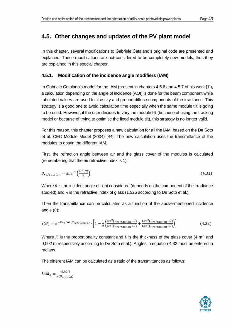
Design and optimisation of the architecture and the orientation of utility-scale photovoltaic power plants Page 43
4.5. Other changes and updates of the PV plant model
In this chapter, several modifications to Gabriele Catalano’s original code are presented and
explained. These modifications are not considered to be completely new models, thus they
are explained in this special chapter.
4.5.1. Modification of the incidence angle modifiers (IAM)
In Gabriele Catalano’s model for the IAM (present in chapters 4.5.6 and 4.5.7 of his work [1]),
a calculation depending on the angle of incidence (AOI) is done for the beam component while
tabulated values are used for the sky and ground-diffuse components of the irradiance. This
strategy is a good one to avoid calculation time especially when the same module tilt is going
to be used. However, if the user decides to vary the module tilt (because of using the tracking
model or because of trying to optimise the fixed module tilt), this strategy is no longer valid.
For this reason, this chapter proposes a new calculation for all the IAM, based on the De Soto
et al. CEC Module Model (2004) [44]. The new calculation uses the transmittance of the
modules to obtain the different IAM.
First, the refraction angle between air and the glass cover of the modules is calculated
(remembering that the air refractive index is 1):
𝜃𝑟𝑒𝑓𝑟𝑎𝑐𝑡𝑖𝑜𝑛 = sin−1 (
𝑠𝑖𝑛(𝜃)
𝑛) (4.31)
Where 𝜃 is the incident angle of light considered (depends on the component of the irradiance
studied) and 𝑛 is the refractive index of glass (1,526 according to De Soto et al.).
Then the transmittance can be calculated as a function of the above-mentioned incidence
angle (𝜃):
𝜏(𝜃) = 𝑒−𝐾𝐿/cos (𝜃𝑟𝑒𝑓𝑟𝑎𝑐𝑡𝑖𝑜𝑛) · [1 −1
2(𝑠𝑖𝑛2(𝜃𝑟𝑒𝑓𝑟𝑎𝑐𝑡𝑖𝑜𝑛−𝜃)
𝑠𝑖𝑛2(𝜃𝑟𝑒𝑓𝑟𝑎𝑐𝑡𝑖𝑜𝑛+𝜃)+𝑡𝑎𝑛2(𝜃𝑟𝑒𝑓𝑟𝑎𝑐𝑡𝑖𝑜𝑛−𝜃)
𝑡𝑎𝑛2(𝜃𝑟𝑒𝑓𝑟𝑎𝑐𝑡𝑖𝑜𝑛+𝜃))] (4.32)
Where 𝐾 is the proportionality constant and 𝐿 is the thickness of the glass cover (4 m-1 and
0,002 m respectively according to De Soto et al.). Angles in equation 4.32 must be entered in
radians.
The different IAM can be calculated as a ratio of the transmittances as follows:
𝐼𝐴𝑀𝑏 =𝜏(𝐴𝑂𝐼)
𝜏(𝜃𝑛𝑜𝑟𝑚𝑎𝑙)

Page 44 Report
𝐼𝐴𝑀𝑠𝑑 =𝜏(𝜃𝑠𝑑)
𝜏(𝜃𝑛𝑜𝑟𝑚𝑎𝑙)
𝐼𝐴𝑀𝑔𝑑 =𝜏(𝜃𝑔𝑑)
𝜏(𝜃𝑛𝑜𝑟𝑚𝑎𝑙) (4.33)
Where 𝐼𝐴𝑀𝑏, 𝐼𝐴𝑀𝑠𝑑, 𝐼𝐴𝑀𝑔𝑑 are the incidence angle modifiers for the beam, sky-diffuse and
ground-diffuse components of the irradiance; 𝐴𝑂𝐼 is the actual angle of incidence between the
module and the sun position; 𝜃𝑠𝑑, 𝜃𝑔𝑑 are the equivalent incidence angles for the sky-diffuse
and ground-diffuse components (to be explained in the following lines) and 𝜃𝑛𝑜𝑟𝑚𝑎𝑙 is the
incidence angle when light incises normal to the module (thus meaning 0º).
As seen, the set of equations 4.33 calculate the different IAM as a ratio between the
transmittance at the actual incidence angle to the incidence angle when light incises normal to
the module. Theoretically, 𝜃𝑛𝑜𝑟𝑚𝑎𝑙 should be set to 0º, but to avoid calculation problems, it is
set to a very small angle close to 0 (1º to be exact). Finally, the equivalent incidence angles
for the sky-diffuse and ground-diffuse are estimated as follows:
𝜃𝑠𝑑 = 59,7 − 0,1388 · 𝛽𝑠 + 0,001497 · 𝛽𝑠2
𝜃𝑔𝑑 = 90 − 0,5788 · 𝛽𝑠 + 0,002693 · 𝛽𝑠2 (4.34)
Both equations present in 4.34 are empirical ones and dependent on the module tilt (𝛽𝑠). In
fact, these equations avoid the problem stated by Catalano on the need to perform an
integration over all the possible directions the sky-diffuse and the ground-diffuse components
can come from.
4.5.2. Inclusion of other DC losses
Following SAM’s approach [2], several complicated DC losses to model have been included
as DC loss factors. The concerned DC losses are:
• Module mismatch loss (𝑳𝒎𝒊𝒔𝒎𝒂𝒕𝒄𝒉): difference in the performance of the modules
connected together induces a DC power loss (modules operate following the lowest
performant module). This loss can be accounted to the order of 2% but depends greatly
on the converter architecture (using power optimisers nullifies this loss and using string
inverter decreases it, while using central inverters maximise it).
• Diodes and connections loss (𝑳𝒅𝒊𝒐𝒅𝒆𝒔,𝒄𝒐𝒏𝒏𝒆𝒄𝒕𝒊𝒐𝒏𝒔): this loss is caused by voltage
drops in the diodes and the connections. SAM estimates it in 0,5%.
• Tracking loss (𝑳𝒕𝒓𝒂𝒄𝒌𝒊𝒏𝒈): when tracking is enabled, this loss accounts for the minimal
energy consumed by tracker mechanisms.
• Nameplate loss (𝑳𝒏𝒂𝒎𝒆𝒑𝒍𝒂𝒕𝒆): this loss refers to a difference between the peak power

Design and optimisation of the architecture and the orientation of utility-scale photovoltaic power plants Page 45
at STC announced by the PV module manufacturers and its real value (normally
lower). Typical causes for this loss vary from traditional degradation to light-induced
degradation (LID, only for the case of p-type mono c-Si) [45].
• Power optimiser loss (𝑳𝒑𝒐𝒘𝒆𝒓_𝒐𝒑𝒕𝒊𝒎𝒊𝒔𝒆𝒓𝒔): only in the case of using module level power
electronics (MLPE) such as power optimiser or micro-inverters, this loss accounts for
their effect.
The corresponding DC power loss factors are calculated as follows:
𝐹𝐷𝐶,𝑖 = 1 − 𝐿𝑖 (4.35)
Where 𝐹𝐷𝐶,𝑖 is DC power loss factor for the respective DC loss 𝐿𝑖. Values of DC loss factor
close to 1 mean small effect of its respective DC loss.
4.5.3. Inclusion of AC losses
In the present work case, since the transformer is considered out of the scope of the project,
only AC wiring losses (𝐿𝐴𝐶_𝑤𝑖𝑟𝑖𝑛𝑔) are accounted. This loss is estimated in 1% and the
corresponding AC power factor loss is calculated in a similar way as in equation 4.35.
4.5.4. Update of the weather files
To provide this simulation tool with a broad spectrum of locations to be selected all around the
world, an update on the weather files have been carried out. The new weather files have been
obtained from SAM’s open source database (thus coming from NREL). For the moment, only
the files tagged as “INTL” (so non-United States locations) can be supported by this simulation
tool. A future update of the simulation tool will try to allow the supportability of files tagged as
“SUNY” (Indian locations) and “TMY2/TMY3” (American locations).
4.5.5. Update of the module and the inverter databases
The module and the inverter database have been updated to the most recent version
(November 2018) with more than 21000 PV modules and more than 7000 inverters available
to be selected. The databases have been obtained from SAM’s last version and are originally
coming from the California Energy Commission (CEC) as a project included in the initiative
“Go Solar California” [46].
4.5.6. Inclusion of the performance ratio (PR) calculation
The performance ratio (PR) is the most adequate quality indicator for PV plants. Since it is a
ratio that considers the actual energy produced with respect to the energy produced in ideal
conditions (so STC/nominal conditions), its result can provide valuable information for PV

Page 46 Report
plants owners about real losses of the system. The PR can be calculated as follows [47]:
𝑃𝑅 =𝑌𝑓
𝑌𝑟=
𝐸𝐴𝐶𝑃0⁄
𝐸𝑔𝑙𝑜𝑏𝑎𝑙𝐺𝑆𝑇𝐶⁄
(4.36)
Where 𝑌𝑓 is the specific yield (kWh/kWp), a measure of the total energy generated per kWp
installed over a certain period of time; 𝑌𝑟 is the reference yield (kWh/kW or peak sun hours),
that represents the energy obtainable at ideal conditions with no losses; 𝐸𝐴𝐶 is the total AC
energy output of the PV plant over a period of time (kWh); 𝑃0 is the nominal capacity of the
PV plant (kWp); 𝐸𝑔𝑙𝑜𝑏𝑎𝑙 is the global POA irradiance reaching the modules (beam + ground-
diffuse + sky-diffuse) (kWh/m2) and 𝐺𝑆𝑇𝐶 is the irradiance at STC (1 kWh/m2).
Usual values for PR vary between 70-80%, with values reaching 90% considered as really
performant PV plants.
4.5.7. Modification of the temperature coefficients
The CEC Module Database includes a coefficient called “adjust” which can be used to modify
the voltage and current temperature coefficients given in the same database. This adjust
parameter allows to adapt the temperature coefficients given in the manufacturers’ datasheets
to a more real value proven by experimental data, according to SAM developers [2]. This
modification can be expressed as:
𝜇𝐼𝑠𝑐 = 𝛼𝐼𝑠𝑐,𝑟𝑒𝑓 · (1 −𝑎𝑑𝑗𝑢𝑠𝑡
100)
𝛽𝑉𝑜𝑐 = 𝛽𝑉𝑜𝑐,𝑟𝑒𝑓 · (1 +𝑎𝑑𝑗𝑢𝑠𝑡
100) (4.37)
Where 𝜇𝐼𝑠𝑐, 𝛽𝑉𝑜𝑐 are the new calculated temperature coefficients for current and voltage; and
𝛼𝐼𝑠𝑐,𝑟𝑒𝑓, 𝛽𝑉𝑜𝑐,𝑟𝑒𝑓 are the temperature coefficients present in the database needed to be
corrected. In any case, the inclusion of this modification results in small variations in the final
energy output of the plant.
4.5.8. Modification of the sizing model
The sizing methodology presented in the work of Gabriele Catalano (chapter 4.8 of his thesis)
has been slightly modified to provide users with more information. Catalano’s work included
the sizing of the modules in series, in parallel and of the number of inverters, taking into account
the limit operating conditions of the PV array (at minimum or maximum operating temperature
or at open-circuit or short-circuit operation, depending on the parameter) and the operating
limits of the inverter (current and voltages).

Design and optimisation of the architecture and the orientation of utility-scale photovoltaic power plants Page 47
This work also includes the nominal inverter ratio as a sizing parameter. This ratio can be
defined as the nominal DC power of the PV array with respect to the nominal AC output of the
inverter. Usual values for this parameter vary between 1-1,3, depending on the system
characteristics. Values under 1 usually mean under sizing of the system.
PV engineers consider acceptable to have up to 30% more DC nominal power than AC
nominal inverter output (Inverter ratio = 1,3) because the DC nominal power is given at STC
conditions, which are hardly occurring in a real-life situation. In any case, this parameter serves
as a tool to choose inverters and the plant layout which are then refined after simulations.

Page 48 Report
5. Validation of the new models
The main goal of this section is to validate two of the models added to the MATLAB code: the
tracking and the self-shading models.
The validation procedure is simple: a year simulation for a specific location is going to be
carried out by SAM (NREL software) and by the MATLAB model used in this work. Both results
are going to be compared and assessed so as to validate the models. The location selected
to validate the models is Seville (the same one which is used in the case studies).
The third main model added to the code (the battery model) cannot be validated by cross-
checking with SAM software. SAM battery model does not allow to simulate the simplified flat-
output operation mode used in this work. However, via the battery case study presented in
chapter 6.2.4, the proper functioning of this model will be assessed.
5.1. Validation of the tracking model
The tracking model can be validated by cross-checking the tracking rotation angle of the PV
modules (defined in chapter 4.2) both in SAM and in the MATLAB code. Figure 14 shows the
evolution of the rotation angle during four different days of the year:
Figure 14. Results comparison for the tracking rotation angle both for SAM and the MATLAB model. Note that the tracking
limit has been set to +-45º. Source: Own.

Design and optimisation of the architecture and the orientation of utility-scale photovoltaic power plants Page 49
As seen in Figure 14, there are no visible differences between the two simulation results. In
this way, the tracking model is confirmed to be valid.
Results for the rest of the year show a similar trend to the one seen in Figure 13. However, for
a few days of the year, a slight difference in the sunrise and sunset times between SAM and
MATLAB simulations can be observed, inducing a slight delay in the tracking angle at the
beginning or at the end of the day. Nevertheless, this difference is not significant in the energy
production since it occurs when radiation values are low (early morning and late evening).
5.2. Validation of the self-shading model
Following a similar approach to chapter 5.2, the self-shading model (non-linear option) has
been validated in Seville. In order to uniform SAM and MATLAB simulations, the following
basic parameters have been set:
• The number of PV modules is 64488. The modules are divided into 5374 strings, each
one of 12 modules in series. The goal of this large number of modules is to simulate a
considerable number of PV rows.
• Each row is composed by 100 modules, in a configuration of 2 modules in the side and
50 in the bottom of the row (see Figure 9 in chapter 4.3 for more information).
• The PV module used is the Jinko Solar JKM320PP-72 with an aspect ratio set at 1,7
(this information is only required to know the module size, not for the module
performance).
• The ground coverage ratio (GCR) has been set at 80%, a large number to force the
maximum self-shading effect possible.
Two yearly simulations have been carried out (one for module portrait configuration and one
for landscape), obtaining similar results throughout the year as evidenced by the simulation
shown on Figure 15 dated January 1st:
(a)

Page 50 Report
Figure 15 shows the results for the self-shading loss factors both for SAM (solid lines) and for
the MATLAB code (dashed lines). As it can be seen, no significant difference can be observed
for the ground and sky-diffuse self-shading loss factors. However, for the DC reduction loss
factor, the MATLAB model estimates larger factors than SAM (thus lower self-shading effect).
The average difference in the DC reduction loss factor is around 1%, meaning that it is
consistent between the prediction error of SAM when compared to real PV plants. This allows
validating the self-shading model (both for portrait and landscape configurations).
Despite the fact that the above-mentioned difference in DC reduction self-shading estimate is
acceptable, several reasons responsible for that are stated in the following lines:
• Differences in the solar time equations: SAM equations differ slightly from PVsyst
equations (the basis for Gabriele Catalano’s original MATLAB code). Moreover, SAM
solar time equations allow for weather datasets composed by different years, which is
not allowed in the MATLAB code (i.e. SAM weather files can include month data
coming from different years to complete a “fictitious” year dataset; and the data year is
a parameter included in the solar time equations).
• Differences between the module size: the self-shading model proposed in this work
uses the module area and the aspect ratio to estimate the module height and width.
On the other hand, SAM is allowed to consider the module height and width if available
in the database, causing a possible variation with respect to the proposed MATLAB.
• Differences in the self-shading model restrictions: equations 4.21 and 4.22 present
slight differences in their restrictions when compared to SAM documentation [2], which
were considered more appropriate by the author of this work.
Figure 15. Results comparison between SAM and the MATLAB code for the self-shading (SS) model: portraid (a)
and landscape (b) module configurations during the 1st of January. Source: Own
(b)

Design and optimisation of the architecture and the orientation of utility-scale photovoltaic power plants Page 51
6. Case studies: Developing a PV utility-scale power
plant in Seville (Spain)
The purpose of this section is to apply the new version of the MATLAB code to the designing
and sizing of utility-scale PV plants. For this reason, several case studies are proposed:
• Comparison between string inverter and central inverter architectures. Moreover,
different DC/AC ratios will be assessed.
• Inclusion of a 1-axis tracking system.
• Self-shading effect on land-use.
• Inclusion of a battery to provide flat-output.
6.1. General assumptions
6.1.1. PV plant location
The case studies are going to be located in Seville, Spain. This location is selected due to its
great weather and solar conditions, as well as an increasing favourable environment to PV
investment, as explained in chapter 3.4.
6.1.2. PV plant size
The PV plant size considered is 100 MW (DC side). This size is of considerable magnitude,
but nothing strange in Europe in the coming years, when utility-scale PV sector is going to be
further developed.
6.1.3. PV modules
The PV modules selected are manufactured by JA Solar (China), one of the top tier cell and
module maker [48]. The model selected is the JAM72S01/PR [49], a 72-cell monocrystalline
PERC module with a peak power of 375 W at STC. Moreover, the module is either compatible
with inverter architectures of 1000 V or 1500 V. For fixed-axis simulations, module tilt is fixed
at 30º.
6.1.4. Inverters
For the string architecture, the market leader in string inverters Huawei is selected. The
model selected is one of its highest power inverters: SUN2000-100-KTL-USH0 [50], with 100
kVA of nominal AC power (100 kW of active power if considering cosф = 1) and a maximum
input voltage of 1500 V.

Page 52 Report
For the central inverter, the well-known German manufacturer SMA is chosen. The model
selected is one of its highest power central inverters: Sunny Central-2500-EV [51], with 2500
kVA of nominal AC power and a maximum input voltage of 1500 V.
6.1.5. LCOE (Levelized Cost of Electricity)
The levelized cost of electricity (€/kWh or €/MWh) can be defined as:
Figure 16. LCOE calculation. Source: Fraunhofer ISE [52].
The equation shown in Figure 16, when applied to PV projects, can be rewritten in the following
way:
𝐿𝐶𝑂𝐸 =𝐶𝐴𝑃𝐸𝑋 + ∑
𝑂𝑃𝐸𝑋𝑡(1 +𝑊𝐴𝐶𝐶)𝑡
𝑛𝑡=1
∑𝐸𝑛𝑒𝑟𝑔𝑦_𝑡𝑜_𝑔𝑟𝑖𝑑𝑡(1 +𝑊𝐴𝐶𝐶)𝑡
𝑛𝑡=1
(6.1)
The life expectancy (for LCOE) calculations is of 25 years.
The WACC (Weighted Average Cost of Capital) is the project average return rate to its
investors (PV projects are financed by a mix of debt and equity). In the Spanish context, it is
estimated at 7% [53].
The yearly energy injected to the grid (𝐸𝑛𝑒𝑟𝑔𝑦_𝑡𝑜_𝑔𝑟𝑖𝑑𝑡) is the output of the MATLAB
simulation for the first year. For the subsequent years, a linear degradation of the output
energy of 0.5% per year [2] is considered. The degradation of the battery (in case it is included)
is also accounted in this factor.
The CAPEX (capital expenditures) is defined by the different components shown in the
following table:
Design and optimisation of the architecture and the orientation of utility-scale photovoltaic power plants Page 53
CAPEX component Value Source
Modules 0,31 EUR/Wp BNEF [15] and PV experts
String inverters 0,05 EUR/WAC BNEF [54]
Central inverters 0,03 EUR/WAC BNEF [54]
BOS (Balance of System) 0,17 EUR/Wp BNEF [15]
Other costs (EPC, land, etc.) 0,30 EUR/ Wp BNEF [15]
Tracker cost (if included) 0,05 EUR/Wp BNEF [38]
Battery cost (if included) 400 EUR/kWh BNEF [55]
Table 1. PV plant CAPEX divided in its components.
Regarding the OPEX, operational expenditures that are accounted every year of the project
lifespan, they can be estimated as follows:
OPEX component Value Source
OPEX PV plant 9500 EUR/MWp BNEF [56] and PV experts
OPEX tracker 900 EUR/MWp BNEF [56] and PV experts
Table 2. PV plant OPEX divided in its components.
6.1.6. PV plant losses
Several PV plant losses are accounted as a percentage of the power output, as explained in
chapters 4.5.2 and 4.5.3.
The module mismatch loss (caused by the performance differences of modules connected
together) is accounted differently depending on the inverter architecture. For string inverters,
it can be estimated at 1% of DC output power loss [57]. For central inverters, it is estimated
slightly higher at 1,25% [57]. This difference is due to the different position of the MPPT
(Maximum Power Point Tracker) which is included within the inverter: the more modules are
controlled together by the same MPPT, the higher is the module mismatch loss. Remember
that using power optimisers or microinverters at module level would nullify this loss.
The diodes and connections loss is estimated at 0,5% of the DC output as suggested by

Page 54 Report
SAM [2].
The tracking loss (when the tracking model is enabled) is estimated at 0,1% of the DC output,
since only takes into account the tracker self-consumption.
The nameplate loss is estimated at 1% of the DC output [58] and accounts for the typical p-
type monocrystalline modules power reduction in the first months due to LID (Light-Induced
Degradation).
The power optimiser loss is set at 0% of the DC output, since no power optimisers are used
in this project (not yet a cost-effective solution for utility-scale, though a great solution for the
residential sector).
The AC wiring loss is estimated at 1% of the AC output [2].
6.1.7. PV plant layout
The following table summarises the plant layout for the different configurations used in the
case studies:
String inverter architecture Central inverter architecture
Modules per string (series) 26 28
Total number of strings 10.250 9.518
Total number of modules 266.500 266.504
DC nominal power (kWp) 99.937,5 kWp 99.939 kWp
Table 3. PV plant layout depending on the inverter architecture selected.
The plant layouts shown in Table 3 have been obtained by sizing the system together with the
corresponding inverter, thus meaning respecting the current and voltage constraints stated in
the datasheets.
The number of inverters to use varies depending on the DC/AC inverter ratio considered in the
case studies. For example, for a DC/AC ratio of 1, 1000 string Huawei inverters are required
while only 42 central SMA inverters are needed. Since several DC/AC ratios are going to be
studied, the number of inverters and strings per inverter (or per array) are going to be further
discussed during the next chapter.

Design and optimisation of the architecture and the orientation of utility-scale photovoltaic power plants Page 55
6.2. Case studies development
6.2.1. String vs central inverter architecture under different DC/AC inverter
ratios
This first case study has the objective to deal with one of the hottest topics in the PV industry:
the choice between string inverters or central inverters, which is basically a fight between
distributed or centralised architectures of PV plants.
String inverters allow for a better control of the plant performance, since the inverter MPPTs
control a lower amount of PV modules, reducing in this way the module mismatch loss.
Moreover, string inverters also allow for a better reliability of the output power, since a failure
in one of the inverters only disconnects a small fraction of the PV plant. On the negative side,
as seen in Table 1, the CAPEX of the PV plant is increased as a consequence of a larger
number of inverters required to be installed.
On the other hand, central inverters benefit from a significant cost advantage due to economies
of scale (here understood as more AC power output packed in one device/inverter) and lower
installation complexity. However, a larger amount of PV modules is controlled by the same
inverter MPPTs, increasing module mismatch losses; and reliability is seriously compromised
Figure 17. Typical image of a PV plant with string inverters (NOTE: The string inverters seen in this figure are of
lower nominal power than the used in this work). Source: Huawei [50].

Page 56 Report
when a single inverter fails.
6.2.1.1. Specific layout of the different configurations proposed
In this case study, three different configurations per each inverter type are proposed, thus
meaning a total of 6 configurations studied (3 string inverter configurations and 3 central
inverter configurations).
Since the goal is to compare and assess differences between string and central inverter but
on the same basis, DC/AC inverter ratios must serve as the common ground for the
comparison (taking into account that the nominal DC power is already fixed at 100 MW).
Bearing that in mind, the following configurations are proposed:
Configuration string 1 Configuration central 1
Inverter type String Central
AC/DC inverter ratio ≈ 1 ≈ 1
Total Number of inverters 1000 42
Modules per string (series) 26 28
Figure 18. Typical image of a PV plant with central inverters. Source: SMA [51].

Design and optimisation of the architecture and the orientation of utility-scale photovoltaic power plants Page 57
Strings per inverter (approx.)1 10 to 11 226 to 227
Total number of strings 10.250 9.518
Total number of modules 266.500 266.504
DC nominal power (kWp) 99.937,5 kWp 99.939 kWp
AC nominal power (kWAC) 100.000 kWAC 98.862,54 kWAC
Table 4. PV plant configurations for a DC/AC inverter ratio of 1.
Configuration string 2 Configuration central 2
Inverter type String Central
AC/DC inverter ratio ≈ 1,15 ≈ 1,15
Total Number of inverters 870 37
Modules per string (series) 26 28
Strings per inverter (approx.)1 11 to 12 257 to 258
Total number of strings 10.250 9.518
Total number of modules 266.500 266.504
DC nominal power (kWp) 99.937,5 kWp 99.939 kWp
AC nominal power (kWAC) 87.000 kWAC 87.093,19 kWAC
Table 5. PV plant configurations for a DC/AC inverter ratio of 1,15.
1 The number of strings per inverter could vary depending on the considered array (e.g. 10 to 11 means that the
inverters in this configuration have either 10 or 11 strings connected to them). This comes as a result of imposing
a total nominal PV plant output, but does not imply technical feasibility problems.

Page 58 Report
Configuration string 3 Configuration central 3
Inverter type String Central
AC/DC inverter ratio ≈ 1,3 ≈ 1,3
Total Number of inverters 769 33
Modules per string (series) 26 28
Strings per inverter (approx.)1 13 to 14 288 to 289
Total number of strings 10.250 9.518
Total number of modules 266.500 266.504
DC nominal power (kWp) 99.937,5 kWp 99.939 kWp
AC nominal power (kWAC) 76.900 kWAC 77.677,71 kWAC
Table 6. PV plant configurations for a DC/AC inverter ratio of 1,3.
Tables 4, 5 and 6 show the different configurations studied depending on the inverter ratio (1,
1,15 and 1,3 respectively). It is interesting to note the AC nominal power row in each table:
while in string configuration cases the AC nominal power matches as a multiple of its inverter
nominal power (100 kW, chapter 6.1.4), the central inverter cases don’t. This is a consequence
of a divergence between the inverter nominal power stated by the manufacturer (2500 kW)
and the CEC Inverter Database (2353,87 kW). This project has decided to follow the CEC
Inverter Database, the one used in the calculations.

Design and optimisation of the architecture and the orientation of utility-scale photovoltaic power plants Page 59
6.2.1.2. Results
Table 7 summarises the results obtained for the different PV plant configurations:
String 1 Central 1 String 2 Central 2 String 3 Central 3
CF (%) 22,83% 22,47% 22,83% 22,46% 22,59% 22,32%
Inverter
losses (%) 1,57% 2,87% 1,57% 2,95% 2,60% 3,53%
Clipping
losses (%) 0% 0% 0,006% ≈ 0% 1,02% 0,48%
PR (-) 0,8491 0,8357 0,8491 0,8351 0,8402 0,83
LCOE
(EUR/MWh) 49,3910 49,0987 49,0525 48,9477 49,3009 49,0921
Energy Y1
(MWh) 170.574,9 167.882,4 170.565,4 167.754,4 168.788,4 166.745,7
Table 7. Summary of the results obtained by the different PV plant configurations (CF-Capacity Factor, PR-
Performance Ratio, LCOE-Levelized Cost of Electricity, Energy Y1-Energy during year 1).
As seen in Table 7, string inverter configurations tend to perform better (higher PR) and
produce more energy than their homologous central inverter configurations. However, when
considering LCOE, central inverters position themselves as the most cost-effective solutions.
These results confirm the working principle of both inverters: string inverters reduce module
mismatch losses but at a higher cost than central inverters. In addition, since the power rating
in central inverters is higher, inverter losses also tend to be higher. (NOTE: Inverter losses
accounts for all the inverter power loss, including efficiency and clipping among others.
However, due to the relevance of clipping losses, they are also presented in the results table).
The best solution of this case study is Configuration central 2, which has the lowest LCOE
among all the solutions: 48,9477 EUR/MWh (or 0,0489 EUR/kWh). This value is in accord with
recent PV projects developed in South Europe and confirms the Spanish PV sector as a
competitive source of electricity.
Configuration central 2 has a DC/AC inverter ratio of 1,15, confirming that under-sizing the
inverter (having a higher DC capacity -modules capacity- than AC capacity -inverters capacity)
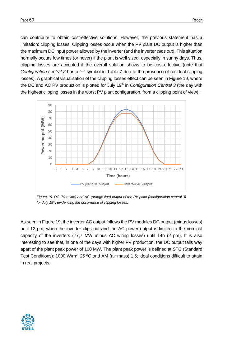
Page 60 Report
can contribute to obtain cost-effective solutions. However, the previous statement has a
limitation: clipping losses. Clipping losses occur when the PV plant DC output is higher than
the maximum DC input power allowed by the inverter (and the inverter clips out). This situation
normally occurs few times (or never) if the plant is well sized, especially in sunny days. Thus,
clipping losses are accepted if the overall solution shows to be cost-effective (note that
Configuration central 2 has a “≈” symbol in Table 7 due to the presence of residual clipping
losses). A graphical visualisation of the clipping losses effect can be seen in Figure 19, where
the DC and AC PV production is plotted for July 19th in Configuration Central 3 (the day with
the highest clipping losses in the worst PV plant configuration, from a clipping point of view):
As seen in Figure 19, the inverter AC output follows the PV modules DC output (minus losses)
until 12 pm, when the inverter clips out and the AC power output is limited to the nominal
capacity of the inverters (77,7 MW minus AC wiring losses) until 14h (2 pm). It is also
interesting to see that, in one of the days with higher PV production, the DC output falls way
apart of the plant peak power of 100 MW. The plant peak power is defined at STC (Standard
Test Conditions): 1000 W/m2, 25 ºC and AM (air mass) 1,5; ideal conditions difficult to attain
in real projects.
Figure 19. DC (blue line) and AC (orange line) output of the PV plant (configuration central 3)
for July 19th, evidencing the occurrence of clipping losses.

Design and optimisation of the architecture and the orientation of utility-scale photovoltaic power plants Page 61
6.2.2. Inclusion of a 1-axis tracking system
The inclusion of tracking devises is another of the hottest topics among PV project developers,
and the focus of this second case study. More exactly, 1-axis tracking systems that follows the
sun from east to west (chapter 4.2 for an exact definition) are studied.
1-axis tracking are expected to become mainstream during the next decade, as stated by the
German PV manufacturers association (VDMA-PV) in its annual ITRPV report (International
Technology Roadmap for Photovoltaic) [20]: 1-axis tracking system will increase their share in
utility-scale PV from around 20% in 2018 to over 50% in 2029.
The reasons for this impressive share growth are rooted to the cost-effectiveness of the
solution: by increasing slightly the system CAPEX and OPEX (Tables 1 and 2), the PV
modules can generate more electricity by following the sun throughout the day. Especially
advantageous is the possibility to start producing electricity earlier in the morning and finishing
the production later in the evening, allowing more production hours and a flatter PV plant
output.
Regarding the 1-axis tracker cost present in Table 1 (0,05 €/Wp), it is important to comment
that this value represents the add on the total system CAPEX. In reality, tracker cost is around
0,10 €/Wp, but this also accounts for the mounting structures. Mounting structures for fixed-
axis systems can be estimated at 0,05 €/Wp, thus the real tracker cost add on total CAPEX
needs to subtract the savings in these mounting structures [38].
The considered best configuration of the previous case study (configuration central 2) will
serve as the baseline for the inclusion of a 1-axis tracking system. Moreover, the tracker angle
of rotation is limited to ±45º, due to mechanical constraints.
6.2.2.1. Results
The following Table 8 shows a comparison between the PV plant (in configuration central 2)
with and without the inclusion of a 1-axis tracking system:
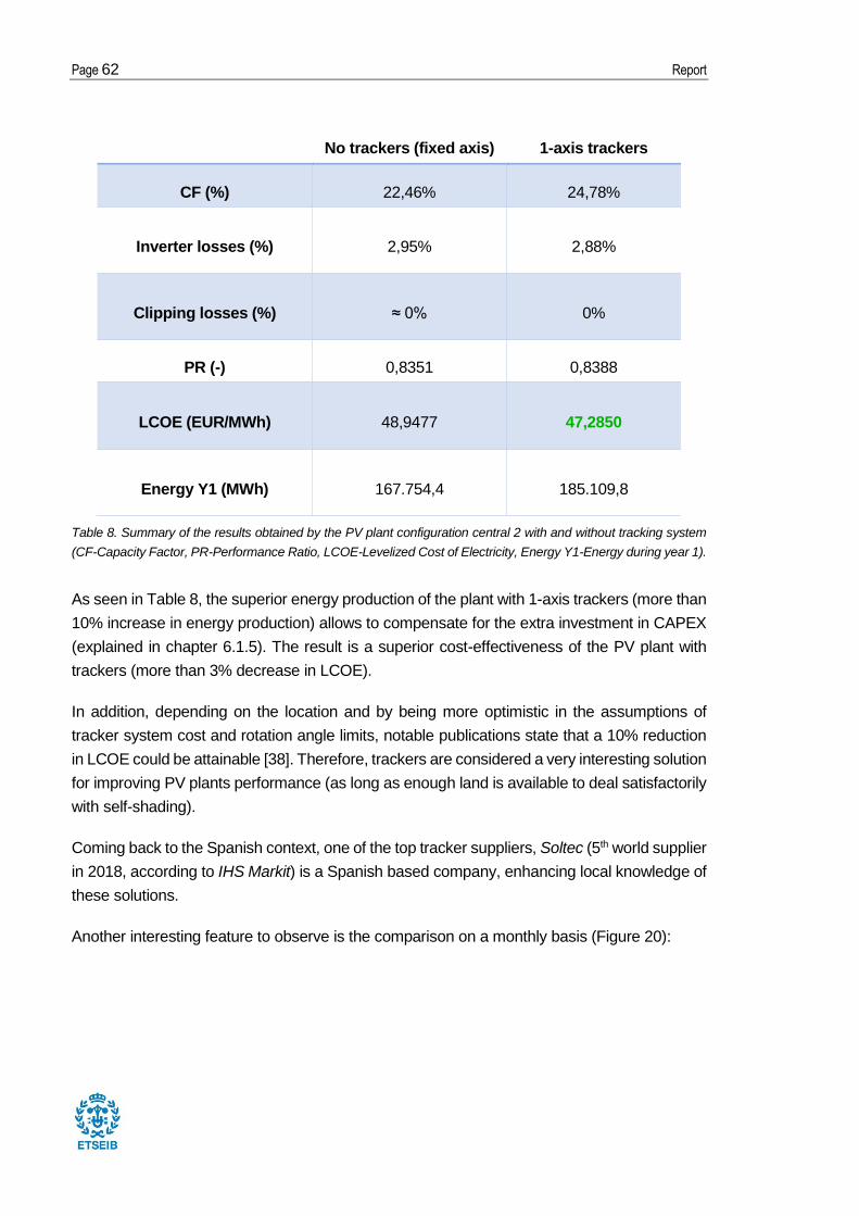
Page 62 Report
No trackers (fixed axis) 1-axis trackers
CF (%) 22,46% 24,78%
Inverter losses (%) 2,95% 2,88%
Clipping losses (%) ≈ 0% 0%
PR (-) 0,8351 0,8388
LCOE (EUR/MWh) 48,9477 47,2850
Energy Y1 (MWh) 167.754,4 185.109,8
Table 8. Summary of the results obtained by the PV plant configuration central 2 with and without tracking system
(CF-Capacity Factor, PR-Performance Ratio, LCOE-Levelized Cost of Electricity, Energy Y1-Energy during year 1).
As seen in Table 8, the superior energy production of the plant with 1-axis trackers (more than
10% increase in energy production) allows to compensate for the extra investment in CAPEX
(explained in chapter 6.1.5). The result is a superior cost-effectiveness of the PV plant with
trackers (more than 3% decrease in LCOE).
In addition, depending on the location and by being more optimistic in the assumptions of
tracker system cost and rotation angle limits, notable publications state that a 10% reduction
in LCOE could be attainable [38]. Therefore, trackers are considered a very interesting solution
for improving PV plants performance (as long as enough land is available to deal satisfactorily
with self-shading).
Coming back to the Spanish context, one of the top tracker suppliers, Soltec (5th world supplier
in 2018, according to IHS Markit) is a Spanish based company, enhancing local knowledge of
these solutions.
Another interesting feature to observe is the comparison on a monthly basis (Figure 20):

Design and optimisation of the architecture and the orientation of utility-scale photovoltaic power plants Page 63
As seen in Figure 20, the tracking option has a superior energy yield during the summer
months (when the sun is higher in the sky). However, during the winter months, the tracking
solution has no advantage at all (even it can produce slightly lower). A lower winter sun altitude
induces a better angle of incidence for fixed-axis modules tilted and facing the south,
translating into a slightly higher energy production. Notwithstanding, the higher production
during summer months allow 1-axis tracking plants to overproduce fixed-axis plants at the end
of the year. Note that this reasoning is valid for the northern hemisphere, but a plant in the
southern hemisphere would have a similar reasoning (inversed from summer and winter
months perspective).
Finally, it is also interesting to observe the comparison in solar production during some
selected day: the summer and the winter solstices (June 21st and December 21st) when the
sun altitude is the highest and the lowest respectively (in the northern hemisphere):
Figure 20. Monthly energy yields for the PV plant with no tracking (blue) and with tracking
(orange).

Page 64 Report
As seen in Figure 21-a, during summer days, the 1-axis tracking PV plant starts producing
electricity earlier in the morning and ends production later in the evening. This fact is relevant,
since the PV plant will be able to help the national power system to ramp up production to
prepare for the night consumption peak.
However, during the winter solstice (Figure 21-b), it can be observed that production with a
tracking system is lower due to a worst angle of incidence (discussed in the previous page).
Fortunately, this only happens few days during the year, concentrated at the end of November,
December and beginning of January, when solar potential is lower in Spain and in Europe.
(a)
(b)
Figure 21. Comparison between the daily AC output of the PV plant with no tracking (blue) and
with tracking (orange): a) June 21st b) December 21st.

Design and optimisation of the architecture and the orientation of utility-scale photovoltaic power plants Page 65
6.2.3. Self-shading effect on land-use
Typically, PV power plants consist of multiple parallel rows of PV modules. Between them, a
certain space is left void to ensure a minimum effect of shading between rows (the so-called
self-shading). However, taking into account that land availability is a finite magnitude, it is
important to find a compromise between self-shading losses and land use. This topic takes a
special relevance in Europe, where the development of utility-scale solar is strongly related to
land availability constraints. Other regions with large extensions of non-populated land, such
as deserts in the Middle East or Northern Africa, are not as exposed to this treat as in the
European case. This is the reason why a self-shading model was considered a key element
to include in the MATLAB simulation code, and its assessment is the focus of this case study.
Again, the considered best inverter configuration in chapter 6.2.1.1 will be the baseline for this
case study (configuration central 2). PV plants with tracking systems are out of the scope of
the present self-shading model, as commented in chapter 2.2. The following Table 9 shows
the general assumptions of the self-shading model (both for portrait and landscape module
configurations), with Figure 22 being a recall of the model nomenclature:
Portrait
configuration
Landscape
configuration
Modules in the side of each row 2 4
Modules in the bottom of each row 250 125
Total number of modules per row 500 500
Total number of rows in the PV plant 533 533
PV module aspect ratio (height to width) 1,7 1,7
Table 9. General assumptions of the self-shading model
Figure 22. Physical configuration of a PV array with its different rows
of modules. Source: SAM [2].

Page 66 Report
The fact of having a different row layout for portrait and landscape configurations is an attempt
to make them comparable from a self-shading point of view: it just does not make sense to
compare each configuration with the same number of modules in the side of the row, since the
portrait case will always produce much more shadows (length of a module is greater than its
width).
An extra parameter is left free to generate the different cases studied: the ground coverage
ratio (GCR, fraction of area occupied by PV modules to the total area). Two different GCR are
going to be tested for both module configurations:
• GCR = 0,3: meaning a space between rows of 12 m (portrait configuration) and 14 m
(landscape configuration).
• GCR = 0,6: meaning a space between rows of 6 m (portrait configuration) and 7 m
(landscape configuration).
Note that the inter-row spacing is indicated as R in Figure 22.
The proposed cases studied in this chapter are only a few of the infinite possible row layouts.
In real PV projects, the inter-row spacing, the row layout and the module configuration are
often decided depending on the location specific characteristics.
6.2.3.1. Results
Table 10 summarises the key indicators of the PV plant for the self-shading case studies
(always considering Configuration central 2 as the base case study):
Portrait
GCR=0,3
Portrait
GCR=0,6
Landscape
GCR=0,3
Landscape
GCR=0,6
CF (%) 22,32% 20,81% 22,32% 21,26%
Inverter losses (%) 2,95% 2,95% 2,95% 2,95%
Clipping losses (%) 0% 0% 0% 0%
PR (-) 0,83 0,7738 0,83 0,7906
LCOE (EUR/MWh) 49,2439 52,8196 49,2385 51,6972
Energy Y1 (MWh) 166.745,4 155.457,3 166.763,5 158.832,3
Table 10. Summary of the results obtained by the PV plant configuration central 2 with the self-shading model
enabled (CF-Capacity Factor, PR-Performance Ratio, LCOE-Levelized Cost of Electricity, Energy Y1-Energy during
year 1).

Design and optimisation of the architecture and the orientation of utility-scale photovoltaic power plants Page 67
Table 10 shows the results obtained when enabling the self-shading model for the different
module and GCR configurations.
As it can be seen, a GCR of 0,3 (i.e. 30% of the land occupied by PV modules) has a low effect
on the plant performance both for portrait and landscape configuration (PR is decreased by a
merely 0,5% and LCOE is worsened by 0,6% roughly). In fact, a 30% occupancy of land is a
popular value between developers of large-scale PV plants if space is available, since self-
shading effect is almost neglectable.
However, when GCR is increased to 60%, annual energy production is reduced by around 6%
for portrait configuration and 5% for landscape due to self-shading losses. This lower energy
production impacts increasing LCOE for both cases - between 2 and 3 EUR/MWh. It is
interesting to observe the impact of the self-shading losses on POA irradiance and DC output
(Table 11). As a quick recall of chapter 4.3, since the case study considers the non-linear
option, self-shading loss factors affect ground and sky-diffuse components directly on the POA
irradiance while beam component is affected on the DC output.
Portrait GCR=0,6 Landscape GCR=0,6
Self-shading loss on irradiance (%) 3,33% 3,33%
Self-shading loss on DC output (%) 4,43% 2,36%
Table 11. Self-shading losses impact (in percentage) on diffuse (loss on irradiance) and beam (loss on DC output)
components for portrait and landscape configurations.
As seen in Table 11, self-shading impact on diffuse components (ground and sky) is almost
the same independently of the module configuration (portrait or landscape). In fact, equations
of the self-shading model for these components of the irradiance (chapter 4.3.2) confirm the
small dependence on module configuration.
On the other hand, self-shading impact on DC output (and thus on the beam component) is
completely dependent on the module configuration. The answer can be found in the non-linear
response of c-Si modules to shading. More precisely, c-Si cells are connected in series to form
modules, with three bypass diodes serving as protection against hotspots. Each bypass diode
protects 1/3 of the module cells, creating “3 submodules”. If only one of these cells is shaded
and performs below the rate of rest, the complete group of cells in the submodule is
disconnected by the diode. As suggested in the beginning of this paragraph, the module
configuration has a great impact on the final output. Let’s imagine a worst-case scenario where
a shade strip appears in the lower part of the modules (Figure 23):

Page 68 Report
In portrait configuration (left in Figure 23), the shade strip affects cells in the lower part of the
module, forcing all bypass diodes to enter conduction mode (setting power output to 0).
On the other hand, in landscape configuration (right in Figure 23), a similar shade only forces
one bypass diode to enter conduction mode, losing 33% of the module rated power (66% of
power output still remains).
Coming back to the present case study, row-to-row self-shading produces similar effects to
the ones shown in Figure 23, reason why landscape configuration has a better performance.
Finally, concerning land use, a dilemma appears: reducing self-shading losses increases
land use and vice versa. The 100 MW plant will occupy around 0,5 km2 in PV modules (same
value for both module configurations). Considering the different ground coverage ratios:
• If GCR=0,3, the PV plant land requirements will be of 1,67 km2.
• If GCR=0,6, the PV plant land requirements will be of 0,84 km2.
Figure 24 shows the evolution of self-shading DC output losses (the most important self-
shading effect) against land use:
Shade Shade
66% Power Output
0% Power Output
Figure 23. Illustration of the power output under shading for portrait (left) and landscape (right) module
configurations. Note that the shade strip produces total shading of the affected cells. Source: Trina Solar
+ Own.

Design and optimisation of the architecture and the orientation of utility-scale photovoltaic power plants Page 69
As it can be seen, Figure 24 evidences the statements discussed in the previous page: the
lower the land use, the more losses due to self-shading. Interestingly, the non-linear shading
effect of c-Si modules is clearly appreciated, as well as the higher vulnerability of portrait
modules to self-shading.
Again, as in the other case studies, there is not a unique choice for module configuration and
row-to-row spacing. It largely depends on the location characteristics and even on the project
developer preferences. In our case, the selected PV plant will be the landscape
configuration with GCR=0,3, since self-shading losses are almost neglectable and land use
is acceptable.
6.2.4. Inclusion of a battery to provide flat-output
Finally, the last case study is focused on the inclusion of a lithium-ion battery to provide a flat-
output response the maximum hours per day. This case study is also of important relevance
when considering that the world’s power systems are increasing the capacity share of
intermittent and difficult to predict renewable energies (such as solar PV). Thus, providing a
more predictable output with a simple battery discharge strategy could play a very important
role in future power systems.
Again, the considered best inverter configuration in chapter 6.2.1.1 will be the baseline for this
case study (configuration central 2). But in this case, to perform a more real simulation, the
self-shading model with landscape configuration and GCR=0,3 is activated.
The general assumptions of the battery are the following ones (see chapter 4.4 for more
information about the parameters):
Figure 24. Self-shading DC los against land use for portrait (red) and landscape configuration.

Page 70 Report
Battery capacity (MWh) 125 MWh 2
SOCinitial (January 1st) (%) 50%
DODmax (%) 90%
Bidirectional converter efficiency (%) 98%
Battery charge efficiency (%) 98%
Battery discharge efficiency (%) 98%
Table 12. General assumptions for the battery model, with typical efficiency values.
With the general parameters of the battery defined (Table 12), two cases are proposed to
study, depending on the flat-output rate desired:
• Desired_flat-output_rate = 50% of the PV plant nominal capacity, thus meaning a
desired flat-output AC power (injected to the grid) of around 50 MW.
• Desired_flat-output_rate = 70% of the PV nominal capacity, thus meaning a desired
flat-output AC power (injected to the grid) of around 70 MW.
The above stated desired flat-outputs rates set the power to be injected to the grid the
maximum number of hours possible (just until the battery runs out of energy).
The battery system cost shown in Table 1 (400 €/kWh) includes, among others: the battery
pack, the battery BOS, the energy management system (EMS), the power conversion systems
(PCS, bidirectional converter), the EPC cost, developer overheads or developer margin [55].
Since main goal of this study is to understand and assess the flat-output response
performance; a 1-year MATLAB simulation will be enough. However, to assess the economic
impact of this option, LCOE calculation is required. This project assumes that battery
degradation over the years follows the same rate as the PV plant’s degradation, 0,5%/year (as
a simplification to avoid performing a 25-year simulation). Being aware of the uncertainty of
this assumption, this works foresees a possible whole battery system replacement during year
15, to account for degradation losses from the cost side of LCOE calculations. The battery
replacement cost in year 15 is estimated at 200 €/kWh, as forecasted by BNEF [55]).
2 The battery capacity has been sized by means of the MATLAB simulation tool with the criterion of
reducing overcharging battery losses to less than ≈1% for the case of Desired_flat-output_rate = 50%.

Design and optimisation of the architecture and the orientation of utility-scale photovoltaic power plants Page 71
6.2.4.1. Results
The following table summarises some interesting indicators for the two flat-outputs proposed:
Flat-output = 50% Flat-output = 70%
LCOE (EUR/MWh) 82,9113 81,1004
Overcharging losses (%) 1,05% 0%
Hours with flat-output, Y1 2502 hours 985 hours
Average hours per day with flat-output, Y1 6,85 hours 2,70 hours
% of the year with flat-output, Y1 29% 11%
Table 13. Summarised results for both cases of flat-output response: 50% and 70% of the PV plant nominal capacity.
It can be seen in Table 13 that LCOEs are slightly different despite having the same cost
structure (CAPEX and OPEX) since the battery capacity is the same for both cases.
The explanation to this fact can be found in overcharging losses (energy burnt during charging
because the battery is already 100% charged): when flat-output is at 50%, 1% of the PV output
is lost due to overcharging. At 70% of flat-output, this loss is nullified, since most of the PV
output is directed to the grid and the battery rests oversized.
In a more general view, it can be observed that both LCOEs are around 30 EUR/MWh higher
than the PV plant without a battery. The conclusion is, that from a cost point of view, batteries
are not still as competitive as PV plants alone. However, batteries can provide services that
must be valued in terms of quality and not of quantity; and maybe in the future these services
could be highly rewarded by system operators (e.g. premium tariffs for providing services,
allowing energy arbitrage, etc.). In addition, utility-scale battery systems will benefit from
economies of scale in Li-ion batteries, induced by the electric vehicle industry, with impressive
cost reductions already forecasted.
From a point of view of the flat-output performance itself, it can be observed that the PV+battery
system could attain the desired output rate for 2502 hours during the year (50% flat-output
case) and 985 hours (70% flat-output), which represents an average of 6,85 and 2,70 hours
of flat-output per day respectively. The difference is obvious: a 50% flat-output rate allows the
system to have enough energy to both charge the battery while yet attaining the desired rate.
However, a 70% flat-output rate makes the system prioritise fulfilling the desired output rate
while not enough energy charges the battery.
A visual description of these facts is shown in Figures 25 a and b, where 3 consecutive days

Page 72 Report
(3rd, 4th and 5th of April) with outstanding PV production are displayed:
Finally, Figure 26 shows the different energy flows that occur in the PV+battery system (for the
4th of April under the 50% flat-output response scenario):
(a)
(b)
Figure 25. For the 3rd, 4th and 5th of April:
a) Power output of the PV system (yellow) and the flat-output responses: 70% (blue) and 50%
(red).
b) Battery state of charge: 70% flat-output case (blue) and 50% flat-output case (red).

Design and optimisation of the architecture and the orientation of utility-scale photovoltaic power plants Page 73
In Figure 26, it can be seen that, during the morning, the PV plant alone satisfies the desired
flat-output. Then, at the beginning of the afternoon, the surplus of PV production is stored in
the battery. Afterwards, during the evening, the battery starts helping the system to reach the
desired flat-output. And from 17:30h, the battery alone starts providing all the output required
to the grid during a couple of hours.
6.3. Case studies conclusions
It has been seen that central inverters are, by a small margin, the most cost-effective solution
when considering large utility-scale PV plants. However, the intense push in string inverters
made by Huawei is starting to pay off: string inverters are already competitive solutions.
Optimising DC/AC inverter ratios is a path to reducing PV systems costs.
The inclusion of trackers can increase considerably the energy output, reducing significantly
the final LCOE. PV plants with trackers must be carefully designed to minimise self-shading
effects. Luckily, tracker manufacturers have already developed back-tracking algorithms.
When considering self-shading in a fixed-axis PV plant, PV developers must optimise their
projects by considering techno-economic indicators but also land-use, since it is going to be a
concern specially in populated regions like Europe and some regions in South-east Asia.
Batteries are not still a great solution economically speaking, but they will be with the
announced cost reductions roadmaps. However, batteries can provide valuable services to the
grid, fundamental when considering renewable energies integration.
Figure 26. System power flows during the 4th of April: total system to grid (dashed blue line), PV
to grid (yellow line), PV to battery (charging, red line) and battery to grid (discharging, green line).

Page 74 Report
7. Planning and budget of the project
This section proposes a brief planning and budget for a 100 MW PV power plant in Seville,
Spain. Since several case studies have been considered in previous section 6, configuration
central 2 (without battery) is selected as the proposed project in this section.
Moreover, since an economic analysis is already provided in the previous section (in the form
of the LCOE, the key techno-economic indicator in the energy industry), the budget is going to
be the only economic topic of this section.
7.1. Planning of the project
Figure 27. Gantt chart for the development of a PV plant project in Seville. Source: Own.
Figure 27 shows the Gantt chart for the PV project studied. Firstly, it is important to note that
there is a previous phase not included in this chart. This phase includes all the project
conception and technical documentation made before the project is officially awarded. In utility-
scale PV plants, it is common to award projects by public national auctions or tenders, where
different companies bid to claim the project. Normally, this previous phase can last for several
years.
In our case, Figure 27 project starts when the awarded company assigns the PV plant
conception to a project developer or so-called EPC (sometimes the same awarded company
is already an EPC). A first stage of project development can last around 7 months, including
site identification, land acquisition, system design, environmental and social assessments or
technology selection.

Design and optimisation of the architecture and the orientation of utility-scale photovoltaic power plants Page 75
In parallel, when enough documentation is collected, the permits and approvals application
to local and national administration starts. This stage can last around 1 year or more depending
on the location (11 months in our project). Sometimes, this stage is considered the nightmare
of developers and one of the riskiest moments of the project.
Once all the permits and approvals are validated, construction can start. Construction
includes from site preparation, to mounting structures and modules installation or wiring
connections. Construction normally lasts between 6 to 12 months depending on the project
characteristics (9 months in our project). Sometimes, certain construction stages can start
before receiving all the permits, but it is not considered in this case.
Finally, the PV plant is delivered. These includes multiple verifications and check-ups to
ensure safety, reliability and performance of the plant. It is estimated in 3 months in this project.
Once all these phases are completed, the PV plant can be brought online. A 2-year timeline
has passed to develop this PV project, which is an average time period for projects of this kind.
7.2. Budget of the project
Table 14 shows the budget for the CAPEX of the 100 MW PV project, taxes excluded:
CAPEX item Unitary cost (EUR/W) Total cost (M€)
PV modules 0,31 EUR/Wp 31 M€
Central inverters (87 MWAC) 0,03 EUR/WAC 2,6 M€
BOS (Balance of System) 0,17 EUR/Wp 17 M€
Other costs (EPC, land, etc.) 0,30 EUR/ Wp 30 M€
TOTAL COSTS -- 80,6 M€
Table 14. Budget of the 100 MW PV project in millions of euros (M€) and excluding taxes.
The capital expenditures of the project account for 80,6 M€, being the PV modules responsible
for more than a third of this amount. This number should be seen as an estimate for similar
projects, since budgetary data is commonly non-disclosed by PV developers
The unitary costs (EUR/W) and their sources are originally presented in chapter 6.1.5 (Table
1). As a recall, other costs include the project development costs (EPC costs), the land
acquisition costs, civil works or even the developer’s margin amongst others.

Page 76 Report
8. Impacts of the project
In this section, both the environmental and socioeconomic impacts are discussed.
8.1. Environmental impact
8.1.1. Equivalent and avoided CO2 emissions
There have been many discussions whether PV technologies are as green as they are said to
be. Most of these discussions being initiated either by the nuclear lobby or the fossil fuels
lobby.
Luckily, experts can easily answer to this controversy by using an impartial tool: the life-cycle
assessment (LCA), which is a carefully detailed methodology to assess the environmental
impact of a product, process or activity. One of the indicators resulting from this analysis is the
carbon footprint, the amount of CO2 equivalent emissions (greenhouse gases emissions)
produced by the product, process or activity studied.
To simplify this assessment in the present work, literature data has been used: a study carried
out by D. Yue, F. You, and S. B. Darling (2014) [59] suggests that the carbon footprint for mono
c-Si modules manufactured in China and installed in Southern Europe amounts to 2,76 kg
CO2-eq/Wp. Openly and frankly, this is a worst-case estimate, since it was assessed in 2014
when China’s energy mix was much darker and manufacturing processes were less efficient
than today. However, for the sake of simplicity and to account for other related emissions of
the PV plant (inverters, BOS, etc.), the present work is going to use this estimate.
The 100 MWp PV plant represents 276.000 t CO2-eq in greenhouse gases emissions. Taking
configuration central 2 case study, the plant will produce around 3950 GWh of electricity all
over the 25 years. This means an average emission per kWh of electricity production of just
0,07 kg CO2-eq/kWh.
On the other hand, the Spanish electricity mix has a 2018 emission factor estimated at 0,321
kg CO2-eq/kWh [60], more than 4 times higher than the one obtained by the PV plant. The
avoided emissions3 thanks to the development of the PV plant account almost for 1 Mt CO2-
eq, which equals to over 16 million of urban trees planted [61]. In fact, after the 5th year the
PV plant has already recovered its initial impact in greenhouse gases emissions.
3 Avoided emissions are defined as the difference between emissions if generating electricity with the
Spanish grid and the emissions of manufacturing the PV modules.

Design and optimisation of the architecture and the orientation of utility-scale photovoltaic power plants Page 77
8.1.2. Land-use
Land-use is one of the most impactful results of a PV plant construction. As seen in chapter
6.2.3, considering a GCR of 0,3 (worst case for land-use), 1,67 km2 of terrain are needed,
which equals the surface of a square measuring 1,3 x 1,3 km (the walking distance from Plaça
Francesc Macià to Passeig the Gràcia taking l’Avinguda Diagonal in Barcelona).
This land occupied by the PV plant cannot be used for other activities, such as agricultural
uses, meaning that some tension could arise from that side. Moreover, if large-scale PV
develops heavily in Spain and in Europe, land availability scarcity could occur. However, by
relying on high-efficiency PV technologies (more electricity production per area) and with good
designing practices, a sustainable PV development in Europe can be ensured.
8.2. Socioeconomic impacts
In general, positive socioeconomic impacts outweigh negative ones. For instance, the local
population will benefit socially and economically from the construction phase, because either
the human force is going to be local or the displaced workers will enrich the local economy.
Moreover, at a national level, the state is going to be provided with a cheap and green source
of energy. Being cheap will allow reducing the Spanish electricity price (in theory, practically
this does not usually occur). And being a green source of energy will allow Spain to accomplish
its emission reduction goals to fight climate change.
Many other positive socioeconomic impacts can be listed, but also some negative impacts, for
instance, the before-mentioned land-use competition or unemployment increase in non-
renewable industries. However, negative impacts can be mitigated with adequate policies and
adaptation to modern times.

Page 78 Report
Conclusions
The original MATLAB PV plant simulation tool has been updated and improved with new
models, submodels, databases and indicators. Amongst others, three important models have
been implemented:
• Tracking system model
• Self-shading model
• Model of the battery (flat-output operation)
The different models added to the code have been validated and used in numerous case
studies.
The case studies have been focused in four important topics of interest to PV plant developers:
• Selection between string and central inverters
• Effects of including trackers
• Land-use and PV plant losses due to self-shading between rows
• Effects of including a battery to provide flat-output response
Central inverters still represent the most cost-effective solution, but the string inverter push is
intense and starts to pay off. DC/AC inverter ratios play an important role in PV plant designing.
Tracker devices usually increase energy yield while reducing LCOE by simply adding a small
add-on in CAPEX.
A dilemma exists between reducing self-shading losses and reducing land-use: self-shading
losses increase as land-use is reduced.
Batteries will play a key role in future power grids, providing services like the one studied in
this project (flat-output response). However, batteries are not still as profitable as PV systems
alone. Cost reduction roadmaps will enhance battery projects profitability.
Finally, it has been seen that PV plants can be developed relatively quick (periods up to 2
years) and their positive impacts largely outweighs their negative ones.
The work in this project could be extended by others, for example, by including a self-shading
model when tracking is considered. This will allow analysing in detail trackers performance.
Furthermore, with a valid tracking self-shading model, designing and optimising backtracking
algorithms will be possible.

Design and optimisation of the architecture and the orientation of utility-scale photovoltaic power plants Page 79
Acknowledgments
Primer de tot, vull agrair a la direcció i al personal (docent i no docent) de l’ETSEIB per aquests
anys de formació que s’acaben amb aquestes línies. Han estat gairebé 8 anys, un grau i dos
màsters i la possibilitat de marxar a l’estranger a estudiar, treballar i viure. És a l’estranger on
un es dóna compte de l’excelent nivell de formació i sobretot d’aquesta multidisciplinaritat i
transversalitat que ens porten a adaptar-nos a diferents condicions i reptes.
També vull agrair al meu tutor, el professor Oriol Gomis, per deixar-me participar en el
desenvolupament d’aquest programa MATLAB començat per un altre estudiant, en Gabriele
Catalano, que des d’aquí aprofito per agrair-li i felicitar-lo pel seu gran treball en la creació del
programa original.
No vull oblidar-me de la meva familia (pares, germana, avis, tiets, cosins) que han estat
“suportant” i “aguantant” tots aquests anys fins al dia d’avui. Especialment els meus pares, qui
crec que finalment estaran satisfets del resultat d’aquests 8 darrers anys.
Et finalement à toi Julie (et à ta famille également !), pour me soutenir et m’encourager pendant
ces derniers mois d’intense travail sur ma thèse.
Page 80 Report
Bibliography
References
[1] Catalano, G. (2018). Development of a model to simulate solar PV plants in MATLAB
with a study on the effects of undersizing the inverter. MSc Thesis. UPC, Barcelona,
Spain. [ONLINE] Available at:
https://upcommons.upc.edu/handle/2117/127357 (Accessed April 1, 2019).
[2] P. Gilman, A. Dobos, N. DiOrio, J. Freeman, S. Janzou, and D. Ryberg. SAM
Photovoltaic Model Technical Reference Update (2018). Colorado, USA. [ONLINE]
Available at:
https://www.nrel.gov/docs/fy18osti/67399.pdf (Accessed April 1, 2019).
[3] PVsyst (2018). First Solar Spectral Correction. Geneva, Switzerland. [ONLINE] Available
at:
http://files.pvsyst.com/help/firstsolar-spectral-correction.htm (Accessed April 1, 2019).
[4] First Solar (2017). Module Characterization: Spectral Response of FS Series PV
Modules. [ONLINE] Available at:
http://www.firstsolar.com/en-EMEA/-/media/First-Solar/Technical-Documents/Series-4-
Energy-Prediction/Spectral-Response-of-FS-Series-PV-Modules.ashx?la=en
(Accessed April 1, 2019).
[5] K. Jäger, O. Isabella, A. Smets, R. van Swaaij, M. Zeman (2014). Solar Energy -
Fundamentals, Technology, and Systems. Delft University of Technology. Netherlands.
[6] M.A. Green (1995). Silicon Solar Cells: Advanced Principles and Practice. Bridge
Printery, Sydney, Australia.
[7] PVmagazine (2019). Global solar demand reached 104 GW in 2018. [ONLINE] Available
at:
https://www.pv-magazine.com/2019/03/06/global-solar-demand-reached-104-gw-in-
2018/ (Accessed April 1, 2019).
[8] PVTECH (2018). Global solar market hit 98.9GW in 2017 - SolarPower Europe.
[ONLINE] Available at:

Design and optimisation of the architecture and the orientation of utility-scale photovoltaic power plants Page 81
https://www.pv-tech.org/news/global-solar-market-hit-98.9-gw-in-2017-solarpower-
europe (Accessed April 1, 2019).
[9] PVmagazine (2019). China installed 44.1 GW of solar in 2018, according to official NEA
data. [ONLINE] Available at:
https://www.pv-magazine.com/2019/01/21/china-installed-44-1-gw-of-solar-in-2018-
according-to-official-nea-data/ (Accessed April 1, 2019).
[10] PVmagazine (2018). BNEF expects 34% fall in PV module prices in 2018. [ONLINE]
Available at:
https://www.pv-magazine.com/2018/06/05/bnef-expects-34-fall-in-pv-module-prices-in-
2018/ (Accessed April 1, 2019).
[11] PVmagazine (2018). EU officially ends MIP for Chinese solar imports. [ONLINE]
Available at:
https://www.pv-magazine.com/2018/08/31/eu-ends-mip-against-chinese/ (Accessed
April 1, 2019).
[12] IEA PVPS, (2018). Trends 2018 in photovoltaic applications. International Energy
Agency (IEA), France. [ONLINE] Available at:
http://www.iea-pvps.org/fileadmin/dam/public/report/statistics/2018_iea-
pvps_report_2018.pdf (Accessed April 1, 2019).
[13] LAZARD (2018). Lazard’s Levelized Cost of Energy Analysis. New York, USA. [ONLINE]
Available at:
https://www.lazard.com/media/450784/lazards-levelized-cost-of-energy-version-120-
vfinal.pdf (Accessed April 1, 2019).
[14] PVmagazine (2018). Solar, wind cheapest source of new generation in major economies
– report. [ONLINE] Available at:
https://www.pv-magazine.com/2018/11/19/solar-wind-cheapest-source-of-new-
generation-in-major-economies-report/ (Accessed April 1, 2019).
[15] BNEF (2018). 2Q 2018 Global PV Market Outlook. Bloomberg New Energy Finance
(BNEF). [ONLINE] Available at: Subscription Service (Accessed May 9, 2018).
[16] Fraunhofer ISE (2018). Photovoltaics report. Fraunhofer Institute for Solar Energy
Systems, ISE, Germany. [ONLINE] Available at:

Page 82 Report
https://www.ise.fraunhofer.de/content/dam/ise/de/documents/publications/studies/Photo
voltaics-Report.pdf (Accessed April 1, 2019).
[17] M.A. Green (2015). The Passivated Emitter and (PERC): From conception to mass
production. University of New South Wales (UNSW). Sydney, Australia. [ONLINE]
Available at:
https://www.sciencedirect.com/science/article/pii/S0927024815003244 (Accessed April
1, 2019).
[18] M. A. Green, Y. Hishikawa, E. D. Dunlop, D. H. Levi, J. Hohl-Ebinger, and A. W. Y. Ho-
Baillie, “Solar cell efficiency tables (version 53),” Prog. Photovoltaics Res. Appl., vol. 27,
no. 1, pp. 3–12, 2018.
[19] W. Shockley, H.J. Queisser (1961). Detailed Balance Limit of Efficiency of p‐n Junction
Solar Cells. Journal of Applied Physics 32, 510.
[20] ITRPV, VDMA (2019). International Technology Roadmap for Photovoltaic (ITRPV):
2018 Results. [ONLINE] Available at:
https://itrpv.vdma.org/ (Accessed April 1, 2019).
[21] First Solar (2019). CdTe Module Manufacturer. Arizona, USA. [ONLINE] Available at:
http://www.firstsolar.com/ (Accessed April 1, 2019).
[22] First Solar (2017). First Solar’s energy advantage in Indian climatic conditions. Arizona,
USA. [ONLINE] Available at:
http://www.firstsolar.com/-/media/First-Solar/Knowledge-Center/Technology-
Advantage/Renewable-Watch---Case-Study.ashx (Accessed April 1, 2019).
[23] Solar Frontier (2019). CIGS Module Manufacturer. Tokyo, Japan. [ONLINE] Available at:
http://www.solar-frontier.com/eng/ (Accessed April 1, 2019).
[24] PV magazine (2017). The weekend read: CIGS is back, back again. [ONLINE] Available
at:
https://www.pv-magazine.com/2018/07/21/the-weekend-read-cigs-is-back-back-again/
(Accessed April 1, 2019).
[25] PV magazine (2017). Momentum builds for HJT. [ONLINE] Available at: https://www.pv-
magazine.com/magazine-archive/momentum-builds-for-hjt/ (Accessed April 1, 2019).
[26] Renewable Market Watch (2018). Renaissance for Solar Photovoltaic (PV) Market in
Spain. [ONLINE] Available at:

Design and optimisation of the architecture and the orientation of utility-scale photovoltaic power plants Page 83
http://renewablemarketwatch.com/news-analysis/265-renaissance-for-solar-
photovoltaic-pv-market-in-spain (Accessed April 1, 2019).
[27] PV magazine (2017). Spain loses its first renewable energy case in international courts.
[ONLINE] Available at:
https://www.pv-magazine.com/2017/05/05/spain-loses-its-first-renewable-energy-case-
in-international-courts/ (Accessed April 1, 2019).
[28] PV magazine (2019). Spain hits 5 GW milestone. [ONLINE] Available at:
https://www.pv-magazine.com/2019/02/05/spain-hits-5-gw-milestone/ (Accessed April 1,
2019).
[29] SolarPower Europe (2019). Spain’s solar market is reignited. [ONLINE] Available at:
http://www.solarpowereurope.org/spains-solar-market-gives-grounds-for-optimism/
(Accessed April 1, 2019).
[30] PV magazine (2018). Four key solar takeaways from Spain’s Genera 2018. [ONLINE]
Available at:
https://www.pv-magazine.com/2018/06/15/four-key-solar-takeaways-from-spains-
genera-2018/ (Accessed April 1, 2019).
[31] PV magazine (2019). “Spain is the hottest PPA market in the world, but auctions are
necessary”. [ONLINE] Available at:
https://www.pv-magazine.com/2019/02/21/spain-is-the-hottest-ppa-market-in-the-world-
but-auctions-are-necessary/ (Accessed April 1, 2019).
[32] Wikipedia (2019). El Dorado. [ONLINE] Available at:
https://en.wikipedia.org/wiki/El_Dorado (Accessed April 1, 2019).
[33] PV magazine (2018). “Flow battery breakthrough?. [ONLINE] Available at:
https://www.pv-magazine.com/magazine-archive/flow-battery-breakthrough/ (Accessed
April 1, 2019).
[34] H. Cho, A. Smith, R. Luck, P.J. Mago (2017). Transient Uncertainty Analysis in Solar
Thermal System Modeling. Missipi State University, USA.
[35] PVsyst (2019). Soiling loss. [ONLINE] Available at:

Page 84 Report
http://files.pvsyst.com/help/soiling_loss.htm (Accessed April 1, 2019).
[36] Sandia National Laboratories (2019). Sandia Inverter Model. [ONLINE] Available at:
https://pvpmc.sandia.gov/modeling-steps/dc-to-ac-conversion/sandia-inverter-model/
(Accessed April 1, 2019).
[37] PV magazine USA (2017). NEXTracker leads global PV tracker market. [ONLINE]
Available at:
https://pv-magazine-usa.com/2017/03/30/nextracker-leads-global-pv-tracker-market/
(Accessed April 1, 2019).
[38] BNEF (2017). Tracking the Sun Has a Bright Future. Bloomberg New Energy Finance
(BNEF). [ONLINE] Available at: Subscription Service (Accessed May 9, 2018).
[39] W. F. Marion and A. P. Dobos (2013). Rotation Angle for the Optimum Tracking of One-
Axis Trackers. NREL, Colorado, USA.
[40] C. Deline, A. Dobos, S.Janzou, J. Meydbray, M. Donovan (2013). A simplified model of
uniform shading in large photovoltaic arrays. NREL, Colorado, USA.
[41] REC Group (2019). REC N-Peak. [ONLINE] Available at:
https://www.recgroup.com/en/products/rec-n-peak-en (Accessed April 1, 2019).
[42] J. Appelbaum, J. Bany (1979). Shadow effect of adjacent solar collectors in large scale
systems. Tel-Aviv University, Israel.
[43] M. De Prada-Gil, J.L. Domínguez-García, L. Trilla, O. Gomis-Bellmunt (2016). Technical
and economic comparison of various electrical collection grid configurations for large
photovoltaic power plants. IREC/CITCEA-UPC, Barcelona, Spain.
[44] W. De Soto, S.A. Klein, W.A. Beckman (2004). Improvement and validation of a model
for photovoltaic array performance. Solar Energy Laboratory, University of Wisconsin-
Madison, USA.
[45] SINOVOLTAICS (2015). PID & LID: Devastating Phenomena for PV plants. [ONLINE]
Available at:
https://sinovoltaics.com/quality-control/pid-lid-devastating-phenomena-pv-plants/
(Accessed April 1, 2019).
[46] Go Solar California (2019). Energy Commission's Solar Equipment Lists. California,

Design and optimisation of the architecture and the orientation of utility-scale photovoltaic power plants Page 85
USA. [ONLINE] Available at:
https://www.gosolarcalifornia.ca.gov/equipment/index.php (Accessed April 1, 2019).
[47] SolarPower Europe (2018). O&M Best Practices Guidelines 3.0. [ONLINE] Available at:
http://www.solarpowereurope.org/wp-content/uploads/2018/12/OM-Best-Practices-
Guidelines-V3.0.pdf (Accessed April 1, 2019).
[48] PVTECH (2019). Top 10 module suppliers in 2018. [ONLINE] Available at:
https://www.pv-tech.org/editors-blog/top-10-solar-module-suppliers-in-2018 (Accessed
April 2, 2019).
[49] JA Solar (2019). 72-Cell Mono PERC Module- JAM72S01/PR. Shanghai, China.
[ONLINE] Available at:
http://www.jasolar.com/index.php?m=content&c=index&a=show&catid=84&id=9
(Accessed April 2, 2019).
[50] HUAWEI (2019). Smart PV String Inverters. Shenzhen, China. [ONLINE] Available at:
http://solar.huawei.com/eu/products (Accessed April 2, 2019).
[51] SMA (2019). SUNNY CENTRAL 2200 / 2475 / 2500-EV / 2750-EV / 3000-EV. Niestetal,
Germany. [ONLINE] Available at:
https://www.sma.de/en/products/solarinverters/sunny-central-2200-2475-2500-ev-2750-
ev-3000-ev.html (Accessed April 2, 2019).
[52] C. Kost, J. N. Mayer, J. Thomsen, N. Hartmann, C. Senkpiel, S. Philipps, S. Nold, S.
Lude, N. Saad, T. Schlegl (2013). Levelized Cost of Electricity Renewable Energy
Technologies Study. Fraunhofer Institute for Solar Energy Systems ISE, Germany.
[53] IRENA (2018). Renewable Power Generation Costs in 2017. International Renewable
Energy Agency (IRENA), Abu Dhabi. [ONLINE] Available at:
http://www.irena.org/publications/2018/Jan/Renewable-power-generation-costs-in-2017
(Accessed April 4, 2018).
[54] BNEF (2018). 2018 Solar Inverter Market Outlook. Bloomberg New Energy Finance
(BNEF). [ONLINE] Available at: Subscription Service (Accessed May 9, 2018).
[55] BNEF (2018). New Energy Outlook 2018. Bloomberg New Energy Finance (BNEF).

Page 86 Report
[ONLINE] Available at: Subscription Service (Accessed June 14, 2018).
[56] BNEF (2018). PV O&M 2017: Providers Push Their Limits for Lower Prices. Bloomberg
New Energy Finance (BNEF). [ONLINE] Available at: Subscription Service (Accessed
May 9, 2018).
[57] PVsyst (2018). How to define the "Mismatch Loss" parameter? [ONLINE] Available at:
https://forum.pvsyst.com/viewtopic.php?t=47 (Accessed April 4, 2019).
[58] PVsyst (2018). LID loss. [ONLINE] Available at:
http://files.pvsyst.com/help/lid_loss.htm (Accessed April 4, 2019).
[59] D. Yue, F. You, and S. B. Darling, “Domestic and overseas manufacturing scenarios of
silicon-based photovoltaics: Life cycle energy and environmental comparative analysis,”
Sol. Energy, vol. 105, pp. 669–678, 2014.
[60] The Catalan Office for Climate Change (OCCC) (2019). Emission factors related to
electrical energy: the electrical mix. Barcelona, Spain. [ONLINE] Available at:
http://canviclimatic.gencat.cat/en/redueix_emissions/com-calcular-emissions-de-
geh/factors_demissio_associats_a_lenergia/ (Accessed April 18, 2019).
[61] United States Environmental Protection Agency (EPA) (2019). Greenhouse Gas
Equivalencies Calculator. United States. [ONLINE] Available at:
https://www.epa.gov/energy/greenhouse-gas-equivalencies-calculator (Accessed April
18, 2019).
