design and properties of self compacting concrete … · the fresh and hardened states alike, still...
TRANSCRIPT

DESIGN AND PROPERTIES OF SELF-
COMPACTING CONCRETE MIXES
AND THEIR SIMULATION IN
THE J-RING TEST
by
Mohammed Shamil Mohammed Abo Dhaheer
B.Sc., M.Sc.
Thesis submitted in candidature for the degree of Doctor of
Philosophy at Cardiff University
School of Engineering
Cardiff University
United Kingdom
November 2016

In the Name of God.
The Most Compassionate and the Most Merciful

DECLARATION AND STATEMENTS
DECLARATION
This work has not previously been accepted in substance for any degree and is not
concurrently submitted in candidature for any degree.
Signed ………………………………… (Mohammed Abo Dhaheer) Date …………..……………
STATEMENT 1
This thesis is being submitted in partial fulfilment of the requirements for the degree of
Doctor of Philosophy.
Signed ………………………………… (Mohammed Abo Dhaheer) Date …………..……………
STATEMENT 2
This thesis is the result of my own independent work/investigations, except where
otherwise stated. Other sources are acknowledged by explicit references.
Signed ………………………………… (Mohammed Abo Dhaheer) Date …………..……………
STATEMENT 3
I hereby give consent for my thesis, if accepted, to be made available for photocopying
and for inter-library loan, and for the title and summary to be made available to outside
organisations.
Signed ………………………………… (Mohammed Abo Dhaheer) Date ………………….……

ACKNOWLEDGEMENT
I would like to express my deepest appreciation to all those who gave me the chance to
complete this thesis. Foremost, I owe a debt of gratitude, which I can never repay, to my
beloved country, Iraq.
I would like to gratefully and sincerely thank my academic supervisor Professor
Karihaloo. It is certainly no exaggeration to say that, this thesis would have been
unthinkable without his guidance and immense support. No mere words can truly
express my appreciation for his assistance during this research.
My profound gratitude is also extended to my co-supervisor Dr. Kulasegaram for being
always helpful, supportive and responsive. I am particularly indebted to him for valuable
discussions and advice I had in accomplishing this thesis.
Appreciation is extended to the Ministry of Higher Education and Scientific Research /
University of Al-Qadisiyah, for the help and support during the study period.
I would like to extend my sincerest thanks and appreciation to my sponsor, the Higher
Committee for Education Development in Iraq (HCED). Without their financial support
and immediate help for different problems I encountered, this work would not have
been achievable.
Special thanks are also extended to the Iraqi Cultural Attaché in London for their
support.
My thanks go to the staff of research office at Cardiff School of Engineering and to the
technical staff of concrete laboratory.
I extend my deepest thanks to my friends who have not left my side throughout this
study and to my office colleagues for their fruitful discussions and cooperation.
A special tribute also goes to my mother, my sisters and the memory of my
unforgettable father.
In closing, I would like to single out my dearest wife and my lovely children, for their
understanding, patience and tremendous support during this study.

SYNOPSIS
Although self-compacting concrete (SCC) has matured beyond laboratory studies and
has now become an industrial product, its characteristics behaviour and performance, in
the fresh and hardened states alike, still need to be thoroughly comprehended. This
thesis presents the results of a study on behaviour of SCC in the fresh and
hardened states. The work was divided into three main parts of research. In the first
part, the focus was to develop a simple and rational method for designing SCC mixes
based on the desired target plastic viscosity and compressive strength of the mix. The
expression for the plastic viscosity of an SCC mix developed using the so-called
micromechanical principles has been exploited to develop this rational method. The
simplicity and usefulness of this method was enhanced by the provision of design charts
for choosing the mix proportions that achieve the mix target plastic viscosity and
compressive strength. Experimental work was performed attesting the validity of this
mix design procedure via a series of SCC mixes in both the fresh and hardened states.
The test mixes were found to meet the necessary self-compacting and the compressive
strength criteria, thus fully validating the proposed mix proportioning method.
Therefore, this method reduces considerably the extent of laboratory work, the testing
time and the materials used.
The second part addressed the other important properties of hardened SCC: specific
fracture energy (𝐺𝐹), direct tensile strength (𝑓𝑐𝑡), critical crack opening (𝑤𝑐),
characteristic length (𝑙𝑐ℎ), which are no less important than the compressive strength.
Combined work with two other PhD candidates (in Cardiff University) has been carried
out in order to get a much clearer picture by investigating in detail the role of several
parameters - coarse aggregate volume, paste volume and strength grade - of SCC mixes
in their 𝐺𝐹, 𝑓𝑐𝑡, 𝑤𝑐 and 𝑙𝑐ℎ. Also addressed in this part is the corresponding bilinear
approximation of the tension softening diagram using a procedure based on the non-
linear hinge model. It is found that all the mentioned properties are dominated by the
coarse aggregate volume (or, conversely the paste volume) in the mix and the mix
grade.
The third part of this thesis is dedicated to simulating the flow of SCC through gaps in
reinforcing bars using the J-ring test. This has been performed by implementing an
incompressible mesh-less smooth particle hydrodynamics (SPH) methodology. A suitable
Bingham-type constitutive model has been coupled with the Lagrangian momentum and
continuity equations to simulate the flow. The capabilities of SPH methodology were
validated by comparing the experimental and simulation results of different SCC mixes.
The comparison showed that the simulations were in very good agreement with
experimental results for all the test mixes. The free surface profiles around the J-ring
bars, the spread at 500 mm diameter and the final flow pattern are all captured
accurately by SPH. In term of segregation assessment, it is revealed that SPH allows the
distribution of large aggregates in the mixes to be examined in order to ensure that they
have not segregated from the mortar. The SPH simulation methodology can therefore
replace the time-consuming laboratory J-ring test, thereby saving time, effort and
materials.

TABLE OF CONTENTS
DECLARATION AND STATEMENTS ................................................................... iii
ACKNOWLEDGEMENT ...................................................................................... iii
SYNOPSIS……. ..................................................................................................... v
TABLE OF CONTENTS ....................................................................................... vii
Introduction ................................................................................... 1
1.1 Introduction ..................................................................................................... 2
1.2 Scope of the research ...................................................................................... 2
1.3 Research objectives ......................................................................................... 4
1.4 Research methodology .................................................................................... 5
1.5 Outline of the thesis ......................................................................................... 6
1.6 Thesis output .................................................................................................... 8
Self-compacting concrete (SCC) .................................................. 10
2.1 Introduction ................................................................................................... 11
2.2 Definition of SCC ............................................................................................ 11
2.3 Development of SCC ...................................................................................... 12
2.4 Advantages and limitations of SCC ................................................................ 12
2.4.1 Advantages of SCC ......................................................................................... 12
2.4.2 Limitations of SCC .......................................................................................... 13
2.5 Functional requirements of SCC .................................................................... 13
2.5.1 Filling ability ................................................................................................... 14

2.5.2 Passing ability ................................................................................................. 15
2.5.3 Segregation resistance ................................................................................... 16
2.6 Approaches to achieve SCC ............................................................................ 16
2.6.1 Powder-type SCC ............................................................................................ 16
2.6.2 VMA-type SCC ................................................................................................ 16
2.6.3 Combination-type SCC ................................................................................... 17
2.7 Constituent materials of SCC ......................................................................... 17
2.7.1 Cement ........................................................................................................... 17
2.7.2 Water ............................................................................................................. 17
2.7.3 Aggregate ....................................................................................................... 18
2.7.4 Powders .......................................................................................................... 18
2.7.5 Chemical Admixtures ..................................................................................... 20
2.8 Proportioning of SCC mixes............................................................................ 21
2.8.1 Comparison of mix proportions of SCC with VC ............................................ 22
2.8.2 Quantity ranges of the constituent materials for SCC ................................... 23
2.8.3 Mix design methods for SCC .......................................................................... 23
2.9 Testing methods for self-compactibility of SCC ............................................. 26
2.9.1 Slump cone test .............................................................................................. 27
2.9.2 J-ring test ........................................................................................................ 28
2.9.3 L-box test ........................................................................................................ 29
2.9.4 V-funnel test ................................................................................................... 30
2.10 Hardened properties of SCC .......................................................................... 31

2.10.1 Compressive Strength .................................................................................... 31
2.10.2 Tensile strength .............................................................................................. 32
2.10.3 Modulus of elasticity ...................................................................................... 32
2.10.4 Fracture mechanics ........................................................................................ 33
2.11 Concluding remarks ....................................................................................... 37
Rheology of SCC and simulation of its flow ................................ 40
3.1 Introduction ................................................................................................... 41
3.2 Rheology of SCC ............................................................................................. 41
3.3 Rheological parameters of fresh SCC ............................................................. 42
3.3.1 Measuring the rheological parameters ......................................................... 43
3.3.2 Models describing SCC flow ........................................................................... 44
3.4 Simulation of SCC flow ................................................................................... 45
3.4.1 Methods for simulating SCC ........................................................................... 46
3.4.2 Numerical solution strategy of simulation techniques .................................. 46
3.4.3 The governing equations used in SCC simulation .......................................... 47
3.4.4 Fundamental approaches describing the physical governing
equations………... ............................................................................................ 48
3.4.5 Domain Discretization .................................................................................... 50
3.4.6 Numerical approximation- Smooth Particle Hydrodynamics (SPH) .............. 51
3.5 Concluding remarks ....................................................................................... 56
Proportioning of SCC mixes based on target plastic viscosity
and compressive strength: mix design procedure ............................. 57

4.1 Introduction ................................................................................................... 58
4.2 Exploitation of an idea: mix design development ......................................... 58
4.3 Target compressive strength ......................................................................... 60
4.4 Target plastic viscosity ................................................................................... 61
4.5 Calculating the plastic viscosity of SCC mixes ................................................ 64
4.6 Basic steps of the proposed mix design method ........................................... 67
4.7 Examples of mix proportioning ...................................................................... 70
4.8 Design charts for mix proportioning of normal and high strength SCC
mixes…………. .................................................................................................. 74
4.9 Examples of the use of design charts............................................................. 82
4.10 Concluding remarks ....................................................................................... 87
Proportioning of SCC mixes based on target plastic viscosity
and compressive strength: experimental validation ......................... 88
5.1 Introduction ................................................................................................... 89
5.2 Materials and mix proportions ...................................................................... 89
5.3 Tests on fresh SCC .......................................................................................... 91
5.3.1 Flow-ability ..................................................................................................... 91
5.3.2 Passing and filling ability ................................................................................ 97
5.4 Testing of hardened SCC .............................................................................. 103
5.5 Concluding remarks ..................................................................................... 104
Influence of mix composition and strength on the fracture
properties of SCC…………. .................................................................... 106

6.1 Introduction ................................................................................................. 107
6.2 Fracture behaviour of SCC ........................................................................... 107
6.3 Parameters describing the fracture behaviour of concrete ........................ 108
6.3.1 Specific fracture energy ............................................................................... 108
6.3.2 Tension softening diagram (TSD) ................................................................. 109
6.4 Theoretical background ............................................................................... 110
6.5 Experimental programme ............................................................................ 114
6.5.1 Materials ...................................................................................................... 114
6.5.2 Mix design .................................................................................................... 114
6.6 Specimen preparation and test procedure .................................................. 116
6.7 Results and discussion ................................................................................. 117
6.8 Bilinear tension softening diagram .............................................................. 123
6.9 Direct and indirect tensile strengths and characteristic length of test SCC
mixes.. .......................................................................................................... 128
6.10 Concluding remarks ..................................................................................... 130
Simulation of SCC flow in the J-ring test using smooth particle
hydrodynamics (SPH) ......................................................................... 131
7.1 Introduction ................................................................................................. 132
7.2 Development of the mixes ........................................................................... 133
7.3 Numerical modelling .................................................................................... 134
7.4 Boundary conditions .................................................................................... 136
7.5 Treatment of particles in the simulated mixes ............................................ 137

7.6 Calculating the assigned volumes of SCC particles ...................................... 138
7.7 Simulation results......................................................................................... 141
7.7.1 Mix flow pattern and t500J ............................................................................ 142
7.7.2 Passing ability ............................................................................................... 144
7.7.3 Assessment of segregation resistance ......................................................... 144
7.8 Remarks on simulation time ........................................................................ 149
7.9 Concluding remarks ..................................................................................... 150
Conclusions and recommendations for further study ............. 151
8.1 Conclusions .................................................................................................. 152
8.2 Recommendations for further study ........................................................... 154
References…. .................................................................................................. 156
Appendix A… .................................................................................................. 177
Appendix B…. ................................................................................................. 185
Appendix C…. ................................................................................................. 198
Appendix D… .................................................................................................. 202
Appendix E…................................................................................................... 209
Appendix F…. .................................................................................................. 216
Appendix G… .................................................................................................. 234

Introduction

Chapter 1 Introduction
2
1.1 Introduction
This chapter highlights the scope of the research, presents the research objectives and
methodology, outlines the structure of the thesis and presents the research output.
1.2 Scope of the research
“Necessity is the mother of invention”. Increasing population and modern cities require
new aspirant structural design ideas and increase the demands on reinforced concrete
structures. The shapes and sections of elements have become more complex and their
reinforcement becomes denser and clustered, which have raised problems of casting,
compacting and filling of concrete elements. With increasing complexity, the durability
problem of concrete structures has become a major issue of interest facing engineers for
many years. Achieving durable concrete structures requires adequate compaction by
skilled labour. During the eighties of the last century, the shortage in skilled site
operatives and its consequential shortage in the quality of construction was a serious
issue in Japan (Okamura and Ouchi, 2003). Consequently, the necessity for a
revolutionary innovation in concrete construction has arisen from the perspectives of
concrete quality assurance and improvement of working conditions. For this reason, a
Japanese researcher (Okamura) in 1986 successfully pioneered what is popularly known
today as “self-compacting concrete” (SCC).
Since its early use in Japan, SCC has now started to be an alternative to vibrated concrete
(VC) across the world as its ability to rationalise the construction systems by offering
several economic and technical advantages over VC (Omran and Khayat, 2016). These
involve: overcoming problems associated with cast-in-situ concrete, ensuring a good
structural performance and robustness, shortening construction time, providing a safe
and healthy working environment by minimizing job-site equipment and noise levels.
Self-compacting concrete is a liquid particle suspension that can compact itself solely by
means of its own weight without the need for vibration effort, and fill the gaps in highly
congested reinforcement and geometrically complicated structural members without any

Chapter 1 Introduction
3
segregation and bleeding (EFNARC, 2005). In other words, it can fulfil the following main
functional requirements: filling ability, passing ability and segregation resistance. To
achieve such requirements, major work should take into account designing appropriate
volume fractions of the mix ingredients. Although SCC has passed from the research
phase into actual application, until recently no unique mix design method has widely
been followed for proportioning SCC mixes, but rather different methods have been
adopted based on a trial and error using time and materials-consuming laboratory tests.
The latter would be significantly reduced if practical guidelines on how to select the most
appropriate volume fractions of mix constituents were introduced in designing SCC.
The volume fractions of the mix constituents, i.e. cement, cement replacement materials,
aggregates, water and admixtures have a significant effect on the rheology of SCC, which
in turn affects its hardened state. Since the SCC main characteristic is flow-ability, its fresh
property cannot be thoroughly comprehended without understanding its rheology. The
quality control and accurate prediction of the SCC rheology is a crucial parameter for the
success of its production.
The quality control and accurate prediction of the SCC flowing behaviour is not a simple
task, particularly in the presence of heavy reinforcement, complex shapes and large size
of aggregate. In this regard, an indispensable and inexpensive approach offering
considerable potential is by performing numerical simulation. This approach will deepen
the understanding of the SCC mix flow behaviour and evaluate its ability to meet the
necessary self-compacting criteria while maintaining adequate suspension and
distribution of coarse particles in the matrix.
Apart from its fresh state, the properties of SCC in its hardened state cannot be
overlooked for its successful proportioning and production. Although the literature is rich
in reporting on SCC, much of the research has primarily focused on the fresh properties,
rather than hardened properties, to produce an SCC mix that possesses the features of
being self-compacting. From an engineering point of view, strength remains the most
important property of hardened concrete as it plays an essential part in its successful
development and gives an indication of its overall quality (Neville, 1995). Thus, to

Chapter 1 Introduction
4
simultaneously achieve the adequate fresh and hardened properties of an SCC mix, the
reliable approach is one which pays implicit attention to its strength along with its
rheological properties, i.e., strength together with rheological properties need to be
imposed as design criteria to successfully produce SCC.
Another important property of hardened SCC, which is no less important than strength, is
its fracture behaviour. An energy based failure theory is needed for this that could be
used in designing cement-based structures since it studies the response and failure of
structures as a consequence of crack initiation and propagation (Karihaloo, 1995). The
most important parameters describing the fracture behaviour of a concrete mix are its
specific fracture energy and the tension softening diagram. They form a basis for the
assessment of the load carrying capacity of cracked concrete structures (Karihaloo, 1995;
Bazant and Planas, 1997). Given the fact that SCC requires relatively large amounts of fine
material and paste but low coarse aggregate content, to control its fundamental
parameters (yield stress and plastic viscosity), its fracture behaviour becomes an issue
and raises concerns among researchers that need to be borne in mind and fully
addressed.
1.3 Research objectives
The main objectives of this thesis are:
❖ firstly, to develop a simple and rational method for designing SCC mixes based on the
desired target plastic viscosity and compressive strength of the mix. The simplicity
and usefulness of this method will be enhanced by the provision of design charts for
choosing the mix proportions that achieve the mix target plastic viscosity and
compressive strength.
❖ secondly, to provide an experimental validation of the proposed mix design method
and to investigate whether the produced SCC mixes meet the necessary self-
compacting criteria in both the fresh and hardened states.
Chapter 1 Introduction
5
❖ thirdly, to examine in detail the role of several compositional parameters - coarse
aggregate volume, paste to solid volume ratio and strength grade - of SCC mixes in
their size-independent fracture energy (𝐺𝐹) and the corresponding bilinear
approximation of the tension softening diagram (TSD).
❖ fourthly, to simulate the non-Newtonian viscous SCC mixes in a standard test
configuration (J-ring test) using the three-dimensional mesh-less smooth particle
hydrodynamic methodology (SPH). This methodology aims to provide a thorough
understanding of whether or not an SCC mix can satisfy the self-compactibility
criterion of passing ability through narrow gaps in reinforcement besides the flow-
ability criterion.
❖ fifthly, to monitor the distribution of coarse aggregate particles in the mixes during
the simulation in order to check whether or not they are homogeneously distributed
after the flow has stopped.
1.4 Research methodology
The above objectives are achieved as follows:
❖ firstly, the expression for the plastic viscosity of an SCC mix developed using
micromechanical principles (Ghanbari and Karihaloo, 2009) will be exploited to
develop the method for proportioning SCC mixes. To aid the user in making an
informed choice of mix constituents, a software program will be developed from
which the design charts are constructed. A regression analysis is performed on the
data collected from many published sources to construct a reliable formula between
water to cementitious material (w/cm) and compressive strength.
❖ secondly, the validity of the proposed mix design method will be proved by preparing
a series of SCC mixes differing in target plastic viscosity and compressive strength. All
these mixes will be extensively tested in the fresh state using the slump cone, J–ring,
L–box and V–funnel apparatus and in the hardened state using compressive strength
test.

Chapter 1 Introduction
6
❖ thirdly, the fracture behaviour of SCC will be experimentally studied on a series of
mixes differing in the coarse aggregate volume, paste volume and strength grade.
The size-dependent fracture energy (𝐺𝑓) will be measured using the RILEM work-of-
fracture test on three point bend specimens containing shallow and deep starter
notches. Then the size-independent fracture energy (𝐺𝐹) will be calculated using the
simplified boundary effect approach (SBE). Finally, the corresponding bilinear
approximation of the tension softening diagram will be obtained using a procedure
based on the non-linear hinge model.
❖ fourthly, the smooth particle hydrodynamics (SPH) approach will be used for
simulating the flow of SCC in J-ring test. SCC is regarded as a non-Newtonian
incompressible fluid whose behaviour is described by a Bingham-type model, which
contains two material properties: the yield stress and the plastic viscosity. For the
investigated mixes, the former is predicted in an inverse manner using the SPH
simulation and the latter is estimated by a micromechanical procedure from the
known plastic viscosity of the paste and the SCC mix proportions. The results of the
numerical simulation will be benchmarked against actual J-ring tests carried out in
the laboratory to examine the efficiency of the proposed methodology (SPH) to
predict accurately the flow behaviour of SCC.
❖ fifthly, the distribution of coarse aggregate in the SCC mix will be simulated and
evaluated along two diametrical planes, in four quadrants and in three concentric
circular regions. The statistics of the coarse aggregate distribution in all cut regions
should be nearly the same to confirm that the flow was homogeneous.
1.5 Outline of the thesis
This thesis is organised into eight chapters, followed by bibliographical references and
appendices. The contents of each chapter can be summarised as follows:
Chapter 1 highlights the scope of the research, presents the research objectives and
methodology, outlines the structure of the thesis and presents the research output.

Chapter 1 Introduction
7
Chapter 2 reviews the properties of SCC, approaches to its achievement, materials used in
its production and their influence on its characteristics in the fresh and hardened states,
proportioning of its constituents and standard tests employed for its assessment. Also
presented in this chapter is a brief review of the mechanical properties of SCC.
Chapter 3 provides a concise review of the rheology of SCC and the methods of simulating
its flow. It also highlights the three-dimensional Lagrangian form of the governing
equations used to model the flow of SCC, which are the mass and momentum
conservation equations. A brief overview of smooth particle hydrodynamic (SPH)
approach is also presented in this chapter.
Chapter 4 describes the systematic steps taken to develop the SCC mix design method
based on the micromechanical procedure. Here, it is worth mentioning that the
micromechanical procedure has enriched this research work far beyond the scope of its
original intended use for the determination of SCC mix plastic viscosity; it forms the
backbone of this rational mix design method. This method has then been enhanced by
the provision of design charts as a guide for proportioning SCC mixes. Several examples
on the use of these charts to proportion mixes with different target plastic viscosity and
compressive strength are given in this chapter.
Chapter 5 is dedicated to the experimental work attesting the validity of the mix design
procedure via a series of SCC mixes in both the fresh and hardened states. To these
mixes, standard tests employed for SCC have been extensively applied.
Chapter 6 presents the results of a combined experimental study on the fracture
behaviour of SCC mixes. This combined work has been carried out with two other PhD
students in order to get a much more clear picture by investigating in detail the role of
several parameters - coarse aggregate volume, paste volume and strength grade - of SCC
mixes in their specific fracture energy (𝐺𝐹). Also given in this chapter is the corresponding
bilinear approximation of the tension softening diagram using a procedure based on the
non-linear hinge model.

Chapter 1 Introduction
8
Chapter 7 describes the three-dimensional SPH method used to simulate all the
developed SCC mixes in the J-ring test. The results of the numerical simulation are
compared with experimental tests carried out in the laboratory to validate the efficiency
of the proposed methodology (SPH) to predict precisely the behaviour of SCC. The
distribution of coarse aggregate in the mix is also evaluated and given in this chapter.
Chapter 8 summarises the conclusions from this research work along with
recommendations for further study.
1.6 Thesis output
The work described in this thesis has been published in different Journals and
conferences. For easy reference, the publications are listed below.
[1] Abo Dhaheer, M.S., Kulasegaram, S. and Karihaloo, B.L. 2016. Simulation of self-
compacting concrete flow in the J-ring test using smoothed particle hydrodynamics
(SPH). Cement and Concrete Research, 89, pp. 27-34.
[2] Abo Dhaheer, M.S., Al-Rubaye, M.M., Alyhya, W.S., Karihaloo, B.L. and
Kulasegaram, S. 2016. Proportioning of self-compacting concrete mixes based on
target plastic viscosity and compressive strength: mix design procedure. Journal of
Sustainable Cement-Based Materials, 5(4), pp. 199–216.
[3] Abo Dhaheer, M.S., Al-Rubaye, M.M., Alyhya, W.S., Karihaloo, B.L. and
Kulasegaram, S. 2016. Proportioning of self-compacting concrete mixes based on
target plastic viscosity and compressive strength: experimental validation. Journal of
Sustainable Cement-Based Materials, 5(4), pp. 217–232.
[4] Abo Dhaheer, M.S., Karihaloo, B.L. and Kulasegaram, S. 2016. Simulation of self-
compacting concrete flow in J-ring test using smoothed particle hydrodynamics. In:
Proceedings of the 24th UK Conference of the Association for Computational
Mechanics in Engineering, ACME, Cardiff, UK.

Chapter 1 Introduction
9
[5] Alyhya, W.S., Abo Dhaheer, M.S., Al-Rubaye M.M., Karihaloo, B.L. and Kulasegaram,
S. 2016. A rational method for the design of self-compacting concrete mixes. In: 8th
International RILEM Symposium on Self-Compacting Concrete, Washington DC, USA,
pp. 85–94.
[6] Alyhya, W.S., Abo Dhaheer, M.S., Al-Rubaye, M.M. and Karihaloo, B.L. 2016.
Influence of mix composition and strength on the fracture properties of self-
compacting concrete. Construction and Building Materials, 110, pp. 312–322.
[7] Alyhya, W.S., Abo Dhaheer, M.S., Al-Rubaye, M.M., Karihaloo, B.L. and
Kulasegaram, S. 2015. A rational method for the design of self-compacting concrete
mixes based on target plastic viscosity and compressive strength. In: 35th Cement
and Concrete Science Conference, CCSC35, Aberdeen, UK.
[8] Al-Rubaye, M.M., Alyhya, W.S., Abo Dhaheer, M.S. and Karihaloo, B.L. 2016.
Influence of composition variations on the fracture behaviour of self-compacting
concrete. In: 21st European Conference on Fracture, ECF21, Catania, Italy.

Self-compacting concrete (SCC)

Chapter 2 Self-compacting concrete (SCC)
11
2.1 Introduction
The key reason why concrete is considered a successful structural material, which has
steadily gained popularity since its inception, is that it can be molded into any desired
structure with the advantages of strength, durability, fire resistance, cost-effectiveness
and on-site manufacturing. Nevertheless, concrete that is cast and compacted under
conditions far from ideal could be prone to flaws such as air voids, honeycombs, lenses of
bleed water and aggregate segregation (Patzák and Bittnar, 2009). These flaws can be a
serious problem in a concrete structure affecting its durability and integrity, irrespective
of the mix strength. The aforementioned shortcomings, especially in structures with
congested reinforcement and restricted areas, can be overcome by the use of self-
compacting concrete (SCC) (Desnerck et al., 2014). This chapter reviews the properties of
SCC, approaches to its achievement, materials used in its production and their influence
on its characteristics in the fresh and hardened states, proportioning of its constituents
and standard tests employed for its assessment. Also presented in this chapter is a brief
review of the mechanical properties of SCC.
2.2 Definition of SCC
Self-compacting concrete (SCC) is a super workable concrete that can compact itself only
by means of its own weight, achieve impressive deformability in its fresh state, fill every
corner, even with restricted areas and geometrically complex shapes, and form a
compact, uniform and void-free mass, while maintaining homogeneity; no vibration is
required and no segregation or bleeding occurs (Desnerck et al., 2014; BS EN 206-9,
2010).
SCC has three fundamental requirements: (1) filling ability which is the characteristic of
SCC to flow under its own weight and to completely fill the formwork; (2) passing ability
which is the characteristic of SCC to flow through and around obstacles such as
reinforcement and narrow openings without blocking, and (3) segregation resistance
which is the characteristic of SCC to remain homogeneous during and after transporting
and placing (BS EN 206-9, 2010; Khayat, 1999).

Chapter 2 Self-compacting concrete (SCC)
12
2.3 Development of SCC
The development of SCC can be divided into two periods: its initial development in Japan
in the mid-1980s and its subsequent spreading into Europe in the late-1990s. In Japan,
the first practical prototype of SCC was produced by 1988, and the first research
publications that looked into the principles required for SCC were around 1989 to 1991
(Goodier, 2003). After these developments, Japan has undergone intensive research in
many places, particularly within the research institutes of large construction companies,
and accordingly, SCC has been used in its many practical applications. The successful
interest and use of SCC in Japan has drawn the attention of many European countries.
The first country in Europe to begin development of SCC was Sweden, from which the
technology spread then to other Scandinavian countries at the end of the 1990s (Goodier,
2003).
Since SCC has gained widespread acceptance in different structural applications,
extensive research work on SCC has been dedicated by different research institutes. To
extract the benefits from its intended use, SCC has to be successfully integrated into the
whole design and construction processes from the viewpoint of making it a standard
concrete. As a result, guidelines and specifications for SCC have been proposed by
individual institutions with the objectives of mix proportions, material requirements and
test methods necessary to produce and test SCC (EFNARC, 2002; EFNARC, 2005; BS EN
206-9, 2010). Simultaneously with the development of its guidelines and specifications,
different parts of the world have embraced SCC and a lot of amazing structures have been
built with this concrete. Examples of structures made with SCC could be found in (Deeb,
2013; Pamnani, 2014; Badry, 2015).
2.4 Advantages and limitations of SCC
2.4.1 Advantages of SCC
SCC has many advantages over VC. These advantages are as follows (Khayat, 1999;
EFNARC, 2005; Okamura and Ouchi, 2003).

Chapter 2 Self-compacting concrete (SCC)
13
➢ Eliminating the need for vibration as it flows through and around obstacles (e.g.
reinforcing steel) under self-weight;
➢ Allowing for the placement of a large amount of reinforcement in small sections,
especially in high-rise buildings;
➢ Improving work environment and safety as it requires fewer workers for transport
and placement of concrete;
➢ Reducing the noise pollution and improving the construction environment in the
absence of concrete vibrating equipment;
➢ Decreasing the construction time and labour cost;
➢ Ensuring a uniform architectural surface finish (appearance of concrete) with little to
no remedial surface work;
➢ Decreasing the permeability and thus, improving strength and durability of concrete.
2.4.2 Limitations of SCC
The possible limitations of using SCC compared with VC are its material costs: it will be
higher than that of VC. However, the reduction of costs caused by better productivity,
shorter construction time and improved working conditions will compensate the higher
material costs and, in many cases, may result in more favourable prices of the final
product. Therefore, when casting in highly congested areas, SCC is more productive,
efficient, and has better constructability than VC.
Another limitation can be related to the nature of SCC: because of its high fluidity,
handling and transporting SCC becomes a bit delicate, although the outstanding results
would overcome these limitations.
2.5 Functional requirements of SCC
In order to be classified as an SCC, the concrete must have the characteristics of filling
ability, passing ability and segregation resistance (Figure 2.1). All these characteristics

Chapter 2 Self-compacting concrete (SCC)
14
should remain throughout the entire construction process (mixing, transporting, handling,
placing and casting).
Figure 2.1: Functional requirements of SCC
2.5.1 Filling ability
Filling ability describes the ability of concrete to flow under its own weight and
completely fill formwork. To achieve the filling ability, the friction between SCC solid
particles (coarse and fine aggregates) has to be reduced. This can be achieved by adding
more water or super-plasticiser. The former could decrease the particle friction and
improve filling ability on the one hand, but on the other hand it leads to segregation in
addition to its consequential reduction in strength and durability. The latter, unlike water
addition, decreases the particle friction by dispersing cement particles and maintains the
deformability and homogeneity of SCC mix.
In order to obtain a better filling ability in SCC, enough paste must be provided to cover
the surface area of the aggregates, and that the excess paste serves to minimize the
friction among the aggregates. Without the paste layer, too much friction would be
generated between the aggregates resulting in extremely limited workability. Figure 2.2
shows the formation of cement paste layers around aggregates.
SCC
Segregation resistance
Filling ability
Passing ability

Chapter 2 Self-compacting concrete (SCC)
15
Figure 2.2: Excess paste layer around aggregates (After: Deeb, 2013)
2.5.2 Passing ability
Passing ability refers to the ability of SCC mix to pass through densely reinforced
structures and narrow spaces, while maintaining good suspension of coarse particles in
the matrix without blocking. The passing ability is related to different parameters.
Increasing paste volume and limiting the size and coarse aggregate content, whose
energy consumption is high, can effectively increase the passing ability and reduce the
risk of blockage. The latter could be attributed to the interaction among aggregate
particles and between the aggregate particles and reinforcement; when concrete
approaches a narrow space, the different flowing velocities of the mortar and coarse
aggregate result in a locally increased content of coarse aggregate (Roussel et al., 2009;
Noguchi et al., 1999). Some aggregates may bridge or arch at small openings which block
the rest of the concrete, as shown in Figure 2.3.
Figure 2.3: Schematic of blocking, aggregates may bridge or arch at small openings which block the rest of
the concrete (After: RILEM TC 174 SCC, 2000)
Also related to the SCC passing ability is paste viscosity: highly viscous paste prevents
localised increases in internal stress due to the approach of coarse aggregate particles
(Okamura and Ouchi, 2003) and therefore increases the passing ability of SCC.
Adding paste Excess paste
thickness
Void
Aggregates

Chapter 2 Self-compacting concrete (SCC)
16
2.5.3 Segregation resistance
Segregation resistance or stability is the concrete’s ability to keep the coarse aggregate
evenly distributed during flow as well as when it is at rest, until the concrete has set.
Enhancement of mix stability can be achieved by providing proper viscosity which is a
consequence of increasing the powder content and/or using a viscosity modifying agent
(VMA). Limiting the size and content of coarse aggregate are also effective in inhibiting
segregation.
It can be mentioned that the above three key requirements are to some extent related
and inter-connected. A variation in one property will lead to a change in one or both of
the others. Both insufficient filling ability and segregation result in unsatisfactory passing
ability. Segregation resistance increases as filling ability increases. SCC is therefore a
trade-off between these parameters (Pamnani, 2014).
2.6 Approaches to achieve SCC
Over the last decade, extensive research has been devoted to achieving self-
compactibility of concrete. Three different approaches have been identified to produce
this type of concrete:
2.6.1 Powder-type SCC
This type of SCC is achieved by using greater amount of cementitious material and filler
along with super-plasticiser at low water to powder ratio (w/p) (Khayat, 1999). Increasing
the powder leads to increased viscosity and improved stability of the fresh concrete. The
flow performance is mainly affected by the super-plasticiser. However, the balance
between flow and stability is very important for the behaviour of fresh concrete.
2.6.2 VMA-type SCC
Addition of VMA enhances the stability of SCC mixes, preventing the concrete from
segregation without increasing powder content (Khayat, 1998; EFNARC, 2005). Similar to

Chapter 2 Self-compacting concrete (SCC)
17
the use of powder in SCC, addition of VMA increases the concrete robustness. However,
from an economical perspective, most VMAs type are expensive and in general more
expensive than powder type using, e.g. limestone filler.
2.6.3 Combination-type SCC
The third main approach of SCC is based on both approaches: powder-type and VMA-type
(EFNARC, 2005). In such type the VMA content is less than that in the VMA-type SCC and
the powder content is less than that in the powder-type SCC. Addition of VMA reduces
the powder needed, and vice versa. The viscosity is provided by the VMA along with the
powder. This type of SCC was reported to have high filling ability, high segregation
resistance and improved robustness (Rozière et al., 2007).
2.7 Constituent materials of SCC
2.7.1 Cement
EFNARC (2005) states that the selection of the type of cement depends on the overall
requirements for the concrete such as strength and durability. Ordinary Portland cement
is most widely used to produce various types of SCC. It is used alone or in combination
with cement replacement materials (CRM). Cement improves the flowing ability of SCC
when used with water to lubricate the aggregates. Cement can also affect the segregation
resistance of SCC by affecting the density of cement paste matrix of concrete.
2.7.2 Water
The amount of water in VC and SCC is important for the properties at the fresh and
hardened stages. However, SCC is more sensitive to the water content in the mix than
traditional vibrated concrete. Adequate water is required for the hydration of cement,
leading to the formation of paste to bind the aggregates. In addition, water is required in
conjunction with super-plasticiser to achieve the self-compactibility of SCC by lubricating

Chapter 2 Self-compacting concrete (SCC)
18
the fine and coarse aggregates in the mix. Typical range of water content in SCC, as per
EFNARC (2005), is 150-210 l/m3.
2.7.3 Aggregate
Aggregate (coarse or fine) characteristics such as size, gradation, shape, volume fraction,
have a significant impact on self-compactibility of SCC (Koehler and Fowler, 2007). With
the reference to the coarse aggregate, it significantly affects the performance of SCC by
influencing its flowing ability, passing ability and segregation resistance as well as its
strength (EFNARC, 2005). All standard sizes of coarse aggregate are generally suitable to
produce SCC. It should be selected in consideration of the performance need for fresh
and hardened concrete (Koehler and Fowler, 2007). Most SCC applications have used
coarse aggregate with a maximum size in the range of 16~20 mm depending on local
availability and particular application (Domone, 2006). Nevertheless, sizes higher than 20
mm could possibly be used. However, SCC with higher volume fraction or maximum size
of coarse aggregate relative to the gap will be more sensitive to segregation, and will
likely need either higher powder content or a viscosity modifying agent (VMA).
The fine aggregates are also a key component of SCC, which plays a major role in its
workability and stability. EFNARC (2005) reports that the effect of fine aggregates on the
fresh properties of SCC mixes is significantly higher than that of coarse aggregate. The
fine aggregates addressed as sand/total aggregate (S/A) ratio is an important material
parameter of SCC that influences its rheological properties (Su et al., 2001).
2.7.4 Powders
During the transportation and placement of SCC the increased flow-ability may cause
segregation and bleeding which can be overcome by enhancing the viscosity of concrete
mix. This is usually supplied by using a high volume fraction of paste, by limiting the
maximum aggregate size or by using viscosity modifying admixtures (VMA) (Khayat,
1999). For this purpose, if only cement and chemical admixtures are used, it will be more
costly, and at the same time lead to more heat of hydration and drying shrinkage. To

Chapter 2 Self-compacting concrete (SCC)
19
avoid such issues, it is necessary to use powder materials, which are greatly beneficial for
concrete properties and durability (Kim et al., 2012). They not only decrease the SCC
materials’ cost but also enhance its particle packing density, self-compactibility and
stability as well as its durability. The term ‘powder’ used in SCC refers to a material of
particle size smaller than 0.125 mm. It will also include this size fraction of the sand.
These materials include cement replacement materials (CRM) and fillers (e.g. limestone
powder).
2.7.4.1 Cement replacement materials (CRM)
CRM are used as a partial replacement of Portland cement in SCC mixes. All CRMs have
two common features; their particle size is smaller or the same as Portland cement
particle and they become involved in the hydration reactions mainly because their ability
to exhibit pozzolanic behaviour. By themselves, pozzolans which contain silica (SiO2) in a
reactive form have little or no cementitious value. However, in a finely divided form and
in the presence of moisture they will chemically react with calcium hydroxide at ordinary
temperatures to form cementitious compounds (Domone and Illston, 2010). The most
common CRMs used are ground granulated blast furnace slag (ggbs), silica fume (SF) and
fly ash (FA). More details of CRMs can be found in (Dinakar et al., 2013a,b; Obla et al.,
2003; Sonebi, 2004; Siddique and Khan, 2011).
2.7.4.2 Fillers
Fillers, such as limestone powder, are used as a portion of total powder content to
enhance certain properties of SCC. It is not a pozzolanic material and its action can be
related to a change in the microstructure of the cement matrix associated with the small
size of the particles (Ye et al., 2007). The filler increases the paste volume required to
achieve the desirable workability of SCC, resulting in an enhancement in the packing
density of powder and in the stability and cohesiveness of fresh SCC (Bosiljkov, 2003;
Topçu and Uǧurlu, 2003).

Chapter 2 Self-compacting concrete (SCC)
20
However, excessive quantities of fine particles can result in a significant rise in the surface
area of powder and an increase in inter-particle friction, due to solid-solid contact, which
may influence the passing ability of the SCC mix and also a substantial rise in the viscosity
(Yahia et al., 2005).
2.7.5 Chemical Admixtures
The most commonly used chemical admixtures in SCC are high range water reducers
(HRWR), or super-plasticiser (SP), and viscosity modifying agent (VMA).
2.7.5.1 High range water reducers (HRWR)
High range water reducer (HRWR) or super-plasticiser (SP) is an essential component of
SCC to provide the necessary workability (Okamura and Ouchi, 2003). The main purpose
of using a super-plasticiser (SP) is to improve the flow-ability of concrete with low water
to binder ratio by deflocculating the cement particles and freeing the trapped water
through their dispersing action, as illustrated in Figure 2.4.
Figure 2.4: Effect of dispersing admixtures in breaking up cement flocs (After: Dransfield, 2003)
SP contributes to the achievement of denser packing and lower porosity in concrete by
increasing the flow-ability, and thus assisting in producing SCCs of high strength and good
durability. For achieving the SCC, an optimum combination of water and SP dosage can be
derived for fixed w/c ratio in concrete (i.e., compressive strength). However, a high SP

Chapter 2 Self-compacting concrete (SCC)
21
amount could cause segregation and bleeding. The new generation super-plasticiser,
which is particularly useful for production of SCC, is Poly-Carboxylate Ether (PCE) based,
although SCC can be made with different types of SP (Assaad et al., 2003; Lachemi et al.,
2003).
2.7.5.2 Viscosity Modifying Agent (VMA)
Viscosity modifying agents (VMA), also known as anti-washout admixtures or anti-
bleeding admixtures, are water-soluble polymers that increase the viscosity of mixing
water and enhance the ability of concrete to retain its constituted suspension. VMA may
also be used as an alternative to increasing the powder content or reducing the water
content of a concrete mix, and mitigating the influences of variations in materials and
proportions in SCC mix, especially when gap-graded aggregates are used (Koehler and
Fowler, 2007). The commonly used viscosity-modifying agent in concrete is welan gum. It
can absorb some of the free water in the system, thus increasing the viscosity of the
cement paste which, in turn, enables the paste to hold aggregate particles in a stable
suspension. As a result, less free water is available for bleeding.
2.8 Proportioning of SCC mixes
Proportioning of SCC can be defined as combining optimum fractions of the constituent
materials to fulfill the requirements of fresh properties (filling ability, passing ability, and
segregation resistance) as well as hardened properties for a particular application
(Desnerck et al., 2014). The complexity of SCC mix proportioning has increased with the
increasing variety of components available for its production: different types of cement
and aggregate (crushed, rounded, etc.), cement replacement materials (ggbs, fly ash,
silica fume, etc.), fillers, chemical admixtures (SP, VMA) (Sandra et al., 2009).
Consequently, different variables must be considered in the proportioning of SCC and
different tests have to be carried out to optimize its constituents. Here, the proportioning
of SCC mix will be discussed in terms of its comparison with VC, quantity ranges of its
constituent materials and the methods developed for its design.

Chapter 2 Self-compacting concrete (SCC)
22
2.8.1 Comparison of mix proportions of SCC with VC
With regard to its proportioning, SCC consists of almost the same constituent materials as
VC, which are cement, aggregates, water and with the addition of chemical and mineral
admixtures (fly ash, silica fume, ggbs, limestone powder, etc.) in different proportions.
However, the reduction of coarse aggregates, the large amount of powder, the
incorporation of SP, the low water to powder (w/p) ratio, are what leads to self-
compactibility. The schematic composition of SCC versus VC is shown in Figure 2.5.
Figure 2.5: The schematic composition of SCC versus VC (After: Okamura and Ouchi, 2003)
There are two main differences in the mix proportioning methods between SCC and VC.
First, the design of VC starts from determining the water to cementicious materials
(w/cm) ratio to satisfy the strength requirement and finishes by the amount of
aggregates. SCC on the other hand is usually proportioned beginning with the fresh
property requirements. Owing to its high cementitious and powder content, which often
ensuring higher strength than is required, designs of SCC usually do not take strength
criterion into account (Ghazi and Al Jadiri, 2010). Second, the fresh and hardened
properties of SCC are more difficult to predict than those of VC and more testing after
design is required. Therefore, the constituent materials of SCC must be carefully
proportioned.
10%
Cement
18%
18% 10%
26%
25%
2 %
2
%
36%
45%
Fin
es
Water + Admixtures
Fine aggregates Coarse aggregates
8%
Air
10%

Chapter 2 Self-compacting concrete (SCC)
23
2.8.2 Quantity ranges of the constituent materials for SCC
Typical ranges of quantities of the constituent materials for producing SCC are given by
EFNARC (2005) (Table 2.1); the actual amounts depend on the desired strength and other
performance requirements.
Table 2.1: Typical range of SCC mix compositions according to EFNARC (2005)
Ingredients Typical range by mass,
kg/m3 Typical range by volume,
litres/m3
Powder (cementitious materials + filler) 380–600 –
Water 150–210 150–210
Coarse aggregate 750–1000 270–360
Water to powder ratio by volume 0.85–1.10
Fine aggregate Typically 48–55% of the total aggregate
Among 56 case studies of SCC applications, Domone (2006) reported that it can be
produced using a wide range of possible constituent materials such that there are still no
clear rules for proportioning SCC mixes. These case studies revealed that coarse
aggregate contents ranged from 28 to 38% of concrete volume, fine aggregate content
varied from 38 to 54% of mortar volume, w/p ratio (by weight) ranged from 0.26 to 0.48,
paste content varied from 30 to 42% of concrete volume, powder content ranged from
445 to 605 kg/m3.
2.8.3 Mix design methods for SCC
Over the years, a number of different mix design methods, based on different principles
(Desnerck et al., 2014; Shi et al., 2015; Koehler and Fowler, 2007) have been proposed by
researchers from various countries around the world. According to their design principles,
these methods could be classified into five categories: (1) empirical design approach; (2)
statistical approach; (3) packing approach; (4) compressive strength approach, and (5)

Chapter 2 Self-compacting concrete (SCC)
24
rheological approach (Shi et al., 2015). The following is a brief overview of these
approaches to each of them an example will be included.
2.8.3.1 Empirical approach
Empirical design method is based on empirical data available for mix parameter to
determine the initial ingredients. The best estimates of the SCC mix proportions for
required properties are performed through several trial mixes and alteration. The
Japanese method was the pioneering work in the SCC mix proportioning based on the
empirical design approach (Shi et al., 2015). It has been adopted and used in many
European countries as a starting point for the development of SCC (Brouwers and Radix,
2005). The main aspects were to fix the coarse aggregate content at 50% of solid volume
and the fine aggregate content at 40% of mortar volume so that self-compactibility can be
achieved easily by adjusting the water-powder ratio (initial value is in the range of 0.9-1
by volume) and super-plasticiser dosage only. In spite of its simplicity, the empirical
design method requires intensive laboratory testing on available raw materials to achieve
satisfactory mix proportions (Shi et al., 2015).
2.8.3.2 Statistical approach
Statistical design approach is used to derive design charts which correlate input mix-
design variables to output material properties, mainly consisting of the measurements of
fresh state properties. Khayat et al. (1999) proposed a mix design method for SCC based
on a statistical model. Their design procedure included five mix parameters: the volume
of coarse aggregate, the cementitious material content, the ratio of water to
cementicious materials, dosage of VMA by mass of water and SP dosage by mass of
binder. The fine aggregate content was varied to achieve the total volume. These
parameters were evaluated and fitted to the results of each measured property (slump
flow, filling ability, V-funnel time and compressive strength) in a statistical manner. It is
however worth mentioning that although the statistical method is valid for a wide range

Chapter 2 Self-compacting concrete (SCC)
25
of SCC mix proportions, establishment of statistical relationships requires intensive
laboratory tests on available raw materials (Shi et al., 2015).
2.8.3.3 Packing approach
In this approach the SCC mix ingredients are obtained by determining the minimum voids
between aggregates according to their packing factor (PF), which is the mass ratio of
closely packed aggregate to that of loosely packed aggregate. The key consideration of
this approach is to fill aggregate voids with an optimum paste volume depending on the
PF value. Su et al. (2001), based on this approach, developed a mix proportion method to
design a medium strength SCC. This method was successfully applied in the Netherlands
(Brouwers and Radix, 2005) and adapted for lightweight SCC in South Korea (Choi et al.,
2006). Given the fact that the design principle of this approach is based on minimum
paste volume, which could save the most expensive constituents (namely cement and
filler), the produced SCC tends to segregate easily, causing a problem for the constructed
structures.
2.8.3.4 Compressive strength approach
An alternative approach for the design of SCC mix was developed based on the
requirement of mix compressive strength. Ghazi and Al Jadiri (2010) constructed a mix
proportioning approach based on two well-known mix design methods, which are the ACI
211.1 (1991) for proportioning VC and the EFNARC (2005) for proportioning SCC. The
requirements of these methods (ACI 211.1 and EFNARC) were combined with certain
modifications to develop this method. The original ACI 211.1 had a range of design
compressive strength of 15 to 40 MPa. This range was widened to cover the
proportioning of SCC with a compressive strength range of 15 to 75 MPa. A modification
on the mix parameters such as coarse aggregate content, cementitious materials, powder
content and w/p ratio were introduced to be within the practical values specified by
EFNARC (2005). It could be mentioned that the compressive strength based approach
gives a clear procedure for proportioning SCC mix ingredients and minimizing the need for

Chapter 2 Self-compacting concrete (SCC)
26
trial mixes. Nevertheless, adjustments to all the mix ingredients are needed to obtain an
optimal mix proportions (Shi et al., 2015).
2.8.3.5 Rheological approach
The rheological properties (plastic viscosity and yield stress) can also be incorporated into
SCC mix design methods, as for instance in the one proposed recently by Karihaloo and
Ghanbari (2012). They have developed a rigorous method for proportioning high strength
SCC mixes with and without steel fibres based on their plastic viscosity. The key
consideration of this method is to exploit the expression for the plastic viscosity of an SCC
mix developed using micro-mechanical principles (Ghanbari and Karihaloo, 2009). Deeb
and Karihaloo (2013) have extended this method to proportioning SCC mixes that contain
traditional coarse aggregate and whose characteristic cube strength ranges between 35
and 100 MPa. Although this method covers a wide range of SCC mixes and reduces the
need for trial mixes, it does not give practical guidelines on how to choose the most
appropriate mix. Also, the compressive strength was not explicitly imposed as a design
criterion in this method.
For more detailed information about SCC mix design methods, we refer the reader to a
very recent work by Shi et al. (2015), where the state of the art review (from 1995 to
2014) on this issue is thoroughly discussed. This review provides valuable scientific basis
for selection of suitable mix design methods of SCC. The procedures, advantages and
drawbacks of the surveyed methods are presented and discussed in this review.
2.9 Testing methods for self-compactibility of SCC
The unique characteristics of SCC do not allow the standard tests employed for VC to be
applied to monitor correctly the fresh properties of the produced SCC. The self-
compactibility tests commonly employed on SCC mixes are briefly described below.

Chapter 2 Self-compacting concrete (SCC)
27
2.9.1 Slump cone test
The slump test is used to assess the deformability of SCC in the absence of obstacles. It is
a simple test such that it can be performed either on site or in laboratory (BS EN 12350-8,
2010). This test measures three different aspects: filling ability, viscosity and resistance to
segregation. The filling ability of SCC is evaluated by measuring the horizontal flow
diameter; the larger the slump flow value, the greater is the ability of SCC mix to fill
formwork under its own weight. Two horizontal perpendicular diameters (d1 and d2) as
illustrated in Figure 2.6 are recorded and the average flow spread diameter (SF) is
calculated.
2
21 ddSF
(2.1)
Figure 2.6: Slump test apparatus
The mix viscosity is assessed by measuring the time needed for SCC to reach 500 mm flow
(t500); the longer the t500, the higher the mix viscosity will be. Two viscosity classes are
introduced: viscosity class 1 (VS1) and viscosity class 2 (VS2) depending on whether t500 < 2
s or ≥ 2 s (BS EN 206-9, 2010).

Chapter 2 Self-compacting concrete (SCC)
28
Moreover, the slump test gives an indication of resistance to segregation in SCC mixes,
which can be detected by visually inspecting the mix periphery after concrete stops to
flow. Segregation is indicated by the occurrence of a halo of paste or unevenly distributed
coarse aggregate in the mix.
2.9.2 J-ring test
The J-ring test in combination with a slump test is used to assess the passing ability of SCC
with or without fibres through gaps in the reinforcement. The apparatus is composed of a
ring with different numbers of vertical reinforcing bars, a slump cone and a rigid plate (BS
EN 12350-12, 2010) as shown in Figure 2.7. Flow spread of the J-ring (SFJ) indicates the
restricted deformability of SCC and can be expressed as:
2
21 ddSFJ
(2.2)
The J-ring can be assessed relative to the flow spread (SFJ) of the same mix using the
slump test as reported in ASTM C 1621/C 1621M (2008). If the difference between spread
diameters (Dflow − DJ-ring) of the two tests is less than 25 mm, then there is no visible
blockage. If it is between 25 and 50 mm, then there is minimal to noticeable blockage.
The SCC passing ability can also be judged in terms of the height difference between the
concrete inside and outside the steel bars of the J-ring using the following equation.
0
2121Δ
4
ΔΔΔΔh
hhhhP
yyxx
J
(2.3)
Here, PJ is the blocking step, ∆h0 is the height measurement at the centre of flow and
∆hx1, ∆hx2, ∆hy1, ∆hy2 are the four measurement heights at positions just outside the J-
ring. The acceptance criterion of SCC passing ability is that the blocking step (PJ) should be
≤ 10 mm (BS EN 206-9, 2010).
The J-ring test can give an indication of resistance to segregation in SCC mixes, which can
be detected by visually inspecting the mix periphery after concrete stops; a ring of
cement paste/mortar in the edge of flow after the concrete has stopped flowing.

Chapter 2 Self-compacting concrete (SCC)
29
Figure 2.7: J-ring test apparatus
2.9.3 L-box test
The L-box test is used to assess the filling and passing ability of SCC. The test is carried out
in accordance with BS EN 12350-10 (2010) and EFNARC (2005). The dimensions of the L-
box are shown in Figure 2.8. The times for the SCC to reach a distance of 200 mm (t200)
and 400 mm (t400) along the horizontal part are measured. Also measured is the height of
concrete at the two ends of the horizontal section of box (H1 and H2) after the concrete
has stopped flowing. The ratio H2/H1 represents the filling ability, and typically, this value
should be 0.8∼1. The passing ability can be detected visually by inspecting the area
around the rebars.

Chapter 2 Self-compacting concrete (SCC)
30
Figure 2.8: L-box test apparatus
2.9.4 V-funnel test
The V-funnel test, which is shown in Figure 2.9, is used to evaluate the viscosity and filling
ability of self-compacting concrete (BS EN 12350-9, 2010; EFNARC, 2005). The V-funnel
test is performed by measuring the time for the concrete to flow out of the funnel under
its own weight. Two viscosity classes are introduced: viscosity class 1 (VF1) and viscosity
class 2 (VF2) depending on whether VF1< 8.0 s or VF2 between 8.0 to 25.0 s (BS EN 206-9,
2010). Segregation resistance of concrete flow can be evaluated by assessing the
homogeneity of concrete flow from the funnel test. In this regards, Alyhya (2016) have
examined (by SPH simulation) the distribution of coarse aggregates in the mix: (1) along
three zones of the V-funnel at different times during the flow, and (2) along three
portions of the collecting container at the outlet of the funnel. He found that, as the
simulation allows the distribution of large coarse aggregates embedded in the
homogeneous mixes to be tracked, it is possible to check whether or not they are
homogeneously distributed during the flow and after the flow has stopped.

Chapter 2 Self-compacting concrete (SCC)
31
Figure 2.9: V-funnel test apparatus
2.10 Hardened properties of SCC
Generally, the hardened behaviour of concrete is governed by its compressive strength.
Numerous papers have been published concerning all aspects of the hardened properties
of SCC, often in comparison with VC (Desnerck et al., 2014; Domone, 2007; Hoffmann and
Leemann, 2005; Persson, 2001). A brief review of the hardened properties is given in this
section. It will emphasise the compressive strength, tensile strength, modulus of rupture
and fracture mechanics properties. The other hardened properties will not be involved as
they are outside the scope of this study.
2.10.1 Compressive Strength
Compressive strength is the key property of hardened concrete that dominates other
mechanical properties and gives an indication of its overall quality (Neville, 1995). Under
given curing conditions, the compressive strength of VC and SCC is mostly determined by
the ratio of water to cementitious material (w/cm). In addition to w/cm ratio, numerous
researchers (Desnerck et al., 2014; Parra, 2011; Vilanova et al., 2011; Domone, 2007;
Hoffmann and Leemannn, 2005; Persson, 2001) have pointed out that compressive

Chapter 2 Self-compacting concrete (SCC)
32
strength of SCC is also influenced by other factors such as type of cement and CRM, use of
materials having pozzolanic activity, type and size of aggregates, type and dosage of
admixtures. However, achieving low compressive strength in SCC is more difficult than
medium and high strength due to the presence of high powder contents.
In general, SCC should exhibit higher compressive strength than VC for a constant w/cm.
This is due to better microstructure and homogeneity in SCC which are the consequences
of significant reduction of segregation and bleeding and reduction of w/p ratio and air
pores. The improved microstructure in SCC is related to the interfacial transition zone
(ITZ) which is denser and significantly more uniform than in VC.
2.10.2 Tensile strength
The tensile strength is one of the key properties that affects the safety, durability and
serviceability of concrete structures (Parra et al., 2011). The tensile strength of SCC is
superior relative to VC (Desnerck et al., 2014; Domone, 2007; Persson, 2001). This is
attributed to the high paste content in SCC and better homogeneity resulting from
vibration free production compared to VC (Nikbin et al., 2014a).
The SCC tensile strength, as VC, has been assessed by splitting, flexural and direct tensile
tests. Many relationships have been built, based on different parameters, to convert
these test results from one to another or as a function of compressive strength (Craeye et
al., 2014; Nikbin et al., 2014a; Parra et al., 2011). This is however not the case for the
direct tensile strength as very limited results are available due to high complexity of this
test. Thus, more test results are necessary to build reliable conclusions with regard to
parametric influences on the direct tensile strength of SCC (Craeye et al., 2014).
2.10.3 Modulus of elasticity
It is known that the modulus of elasticity of concrete depends on the modulus of elasticity
of the individual mix ingredients. It increases with high content of aggregates, whereas it

Chapter 2 Self-compacting concrete (SCC)
33
decreases with increasing paste volume and increasing porosity (Neville, 1995). However,
the increase in the SCC modulus of elasticity due to the decrease in porosity cannot
compensate for the reduction induced by the lowering of coarse aggregate content
and/or increasing paste volume. Accordingly, lower values of modulus of elasticity can be
expected for SCC, as it has relatively higher content of paste and lower content of coarse
aggregate than VC.
Craeye et al. (2014) reported that due to the significant contribution of aggregates to the
overall stiffness of concrete, it is expected that SCC, with its higher paste volume, tends to
reach a slightly lower modulus of elasticity than VC. Similar conclusions have been drawn
by other researchers (Desnerck et al., 2014; Domone, 2007; Nikbin et al., 2014a; Parra et
al., 2011).
2.10.4 Fracture mechanics
Concrete structure, because of its heterogeneity, can be prone to flaws such as irregularly
distributed pockets of entrapped air voids, lenses of bleed water and shrinkage cracks,
even prior to the application of load. These flaws grow stably under external load,
coalesce with existing or newly-formed small cracks until large fractures are formed
which cause the collapse of the structure. When a load is applied there will be high stress
concentrations around these cracks, higher than those at other points within the
structure. These cracks propagate during service and can be a serious problem in such
structures. Since it studies the response and failure of structures as a consequence of
crack initiation and propagation, fracture mechanics provides an energy based failure
theory that could be used in designing cement-based structures (Karihaloo, 1995).
2.10.4.1 Linear elastic fracture mechanics (LEFM)
Linear elastic fracture mechanics (LEFM) has been available since 1920 (Karihaloo, 1995).
However, it is absent from the Codes because the Griffith fracture theory is only
applicable to elastic homogeneous brittle materials such as glass (Karihaloo, 1995).
Thought to be a brittle material, attempts were made to apply LEFM to concrete, but

Chapter 2 Self-compacting concrete (SCC)
34
these proved unsuccessful due to the fact that cement-based materials indeed show a
different response. For a quasi-brittle material like concrete, a substantial non-linearity
exists before the maximum stress is reached (region AB in Figure 2.10a). This is the strain
hardening response of the material. There is also a region of softening after the
attainment of the maximum load (region BC in Figure 2.10a). These are mainly a result of
randomly formed micro-cracks. The tail region of tension softening (region CD in Figure
2.10a) is caused by the aggregate interlock and other frictional effects.
The pre-peak non-linearity has only a minor impact on the fracture behaviour of concrete.
In fact, the major impact comes from the tension softening response because it reduces
the flux of energy which can be released into the crack tip and thereby leads to an
increase in the fracture surface area. Therefore, the LEFM application to concrete
structures is limited, due to the presence of the tension softening response. In other
words, the fracture behaviour of concrete is affected by the formation of an extensive
fracture process zone (FPZ) ahead of the pre-existing crack (Figure 2.10b).
Figure 2.10: Typical load-deformation response of a quasi-brittle material in tension/flexure (a) and the
fracture process zone ahead of the real traction-free crack (b) (After: Karihaloo, 1995).
(a)
(b)

Chapter 2 Self-compacting concrete (SCC)
35
2.10.4.2 Fracture process zone (FPZ)
The fracture process zone (FPZ) is defined as the inelastic zone around the crack tip and
corresponds to the region of tension softening of the load-deformation curve (Figure
2.10). Many mechanisms that are responsible for fracture process in concrete are related
to the development of the fracture process zone. Some of these mechanisms are
indicated in Figure 2.11 such as, micro-cracking at aggregate due to the presence of a
macro-crack, de-bonding and micro-cracking, coalescence of de-bond crack with a macro-
crack and the crack bridging.
Figure 2.11: Schematic representation of the fracture process zone (After: Karihaloo, 1995).
Fracture behaviour of concrete is significantly influenced by the FPZ. Since the FPZ
consumes a substantial amount of the energy supplied by the applied load, a crack can
propagate steadily prior to failure. The FPZ is responsible for the quasi-brittle fracture
response of concrete after the peak load. Since some parts of crack surfaces may still be
in contact after cracking, stress gradually decreases after the peak load, and a softening
type of concrete stress-strain relationship is obtained.

Chapter 2 Self-compacting concrete (SCC)
36
2.10.4.3 Nonlinear fracture mechanics (NLFM)
LEFM is not applicable to concrete due to the existence of the inelastic toughening
mechanisms (i.e. FPZ) that appear around a crack when it propagates. A fracture theory
capable to describe the material softening process that takes place in the fracture process
zone must be a non-linear fracture theory (Karihaloo, 1995). The first non-linear theory of
fracture mechanics for quasi-brittle materials like concrete is the fictitious crack model
(FCM) proposed by Hillerborg et al. (1976). Bažant (1984) proposed the second non-linear
theory of fracture, which is the crack band model. The two non-linear theories were
covered in detail by Karihaloo (1995).
The fictitious crack model set a benchmark for fracture mechanics of concrete and is
widely used in various applications (Hu and Wittmann, 2000). The applications of this
model require the knowledge of two important parameters: the size-independent
fracture energy, 𝐺𝐹 and the tension softening diagram, σ(w) of the concrete mix. These
parameters form the basis for the assessment of the load carrying capacity of cracked
concrete structures (Karihaloo, 1995; Bazant and Planas, 1997).
𝐺𝐹 can be simply calculated using the simplified boundary effect (SBE) formalism (Abdalla
and Karihaloo, 2003) from notched three-point bend test of single size specimens with
only two distinctly-different notch to depth ratios, while σ(w) could ideally be obtained
from the direct tension test. However, as the determination of σ(w) using such test is not
a simple task, it is often approximated by a bilinear relationship whose parameters are
determined in an inverse manner by matching the experimental load-displacement curve
of a notched three-point bend beam. To avoid unnecessary duplication, detailed
information about the above parameters will be presented and discussed together with
results from this study in Chapter 6.
2.10.4.4 Fracture behaviour of SCC versus VC
The fracture behaviour of concrete, as a specific type of composite material, is
significantly influenced by the properties of matrix (Akçaoǧlu et al., 2004), which in turn
are governed by the mix ingredients in VC and SCC, as well. Based on the experimental

Chapter 2 Self-compacting concrete (SCC)
37
results obtained from different researchers (Karihaloo, 1995; Akcay et al., 2012; Prokopski
and Langier, 2000), reduction of the aggregate size and content in VC leads to decrease in
fracture energy. This is the consequence of the decrease in aggregate bridging and
interlocking across the crack resulting in the reduction of energy absorption. In SCC,
concerns have been raised among researchers as it may have inferior fracture behaviour
compared to VC (Beygi et al., 2014a,b,c; Domone, 2006). This is primarily due to the fact
that SCC requires comparatively low coarse aggregate content but large amounts of fine
material and paste in order to control its fundamental parameters (yield stress and plastic
viscosity).
The differences in SCC mix composition lead to change in its pore structure, resulting in
modified mechanical behaviour, especially fracture properties, and consequently
different cracking behaviour. These conclusions were confirmed by previous studies
(Beygi et al., 2014a,b,c; Nikbin et al., 2014b,c; Cifuentes and Karihaloo, 2013; Beygi et al.,
2013a; Rozière et al., 2007). These studies, apart from the study of Cifuentes and
Karihaloo (2013), were indeed based on the size-dependent specific fracture energy (𝐺𝑓),
not on the true fracture energy (size-independent fracture energy (𝐺𝐹)). However, since a
lack of adequate knowledge on the SCC fracture behaviour (specifically 𝐺𝐹), due to a
limited amount of test results from literature, the use of the fracture assumptions and
relations that are valid for VC might be risky for SCC (Beygi et al., 2014c).
2.11 Concluding remarks
Self-compacting concrete, which is characterised in its fresh state by high flow-ability and
rheological stability, has excellent applicability for elements with complicated shapes and
congested reinforcement. It has rationalised the construction systems by offering several
economic and technical advantages over VC. A concrete mix can only be classified as SCC
if its main functional requirements (filling ability, passing ability and segregation
resistance) are fulfilled. These are mainly achieved by exploiting the benefits of super-
plasticisers (SP) and viscosity modifying agents (VMA) (if required), cement replacement
material (CRM) and fillers. The above three key requirements are to some extent related

Chapter 2 Self-compacting concrete (SCC)
38
and inter-connected. In other words, SCC is a trade-off between these parameters; a
variation in one property will lead to a change in one or both of the others.
Since the SCC requirements are mostly influenced by the fractions of the mix ingredients,
it becomes crucial to develop an appropriate procedure for its proportioning. A review of
the mix design methods indicates that SCC can be designed using a wide range of possible
constituent materials such that there is no unique mix design method has widely been
followed for proportioning SCC mixes. To all of the surveyed methods, a significant
number of time and material-consuming trial mixes are inevitably needed before an
optimum mix proportion is reached. However, in most of the reviewed methods, it should
be pointed out that attention has primarily been paid to the fresh properties, rather than
hardened properties, to produce an SCC mix that possesses the features of being self-
compacting.
Recently, a rigorous method for proportioning high strength SCC mixes with and without
steel fibres has been developed. The key consideration of this method is to exploit the
expression for the plastic viscosity of an SCC mix developed using micro-mechanical
principles. Although this method covers a wide range of SCC mixes and reduces the need
for trial mixes, it does not give practical guidelines on how to choose the most
appropriate mix. In addition, the compressive strength was not explicitly imposed as a
design criterion in this method. As a result, there is a scope in this study (Chapters 4 and
5) to overcome the shortcomings of this method, in which practical guidelines in the form
of design charts will be developed as a guide for proportioning SCC mixes.
A review of the literature concerning the hardened properties shows that SCC mixes are
often, but not always, accompanied with improvements in these properties. The
compressive and tensile strengths of SCC are always higher than that of VC due to the
improvement in mix microstructures. Many relationships have been built for VC to
convert the test results of compressive and tensile strength (which is assessed by
splitting, flexural and direct tensile strength) from one to another. However, it is not quite
clear whether these conversion factors are still valid for SCC and therefore, more
experimental results are necessary to reach reliable conclusions. In this thesis, we will
develop relationships between the direct and indirect tensile strength of SCC mixes of

Chapter 2 Self-compacting concrete (SCC)
39
different paste to solid ratio, coarse aggregate volume and mix grades. This will give a
better understanding of the contribution of these compositional parameters on the
tensile strength of SCC.
Based on the results obtained from different studies, it is indicated that SCC, with its high
paste volume and low coarse aggregate contents, tends to have a lower fracture energy
than VC, which raises concerns among researchers. A limited number of studies has
debated the parameters affecting the SCC fracture behaviour (specifically the size-
independent fracture energy, 𝐺𝐹) such as coarse aggregate content, paste volume and
strength grade. In Chapter 6, we will examine in detail the role of these compositional
parameters of SCC mixes in their 𝐺𝐹 and the corresponding bilinear approximation of the
tension softening diagram (TSD).
The next chapter will look concisely at the rheology of SCC and simulating its flow, which
are the two key issues in the scope of this study.

Rheology of SCC and simulation of its flow

Chapter 3 Rheology of SCC and simulation of its flow– A concise review
41
3.1 Introduction
A key phase, when producing SCC, lies in understanding its workability to provide a
quantitative fundamental way of characterising its self-compactibility so as to obtain
adequate properties of fresh concrete. Without understanding this property, SCC will
continue to be designed by trial and error to satisfy the performance required for a
particular application. Several tools are available to assess the workability of SCC. These
tools can be classified into three categories (Tattersall, 1991): qualitative assessment,
quantitative empirical assessment and quantitative fundamental assessment. In the
previous chapter, the qualitative assessment of SCC was reviewed via its functional
requirements (flow-ability, passing ability and stability), and quantitative empirical
assessment via classical tests recommended by the British standard (BS EN 206-9, 2010)
such as slump flow, J-ring, L-box and V-funnel tests. In this chapter, the SCC workability
will be quantitatively reviewed in terms of its fundamental rheological properties, which
is crucial for the success of its production. However, the prediction of SCC rheological
behaviour is not a simple task, particularly in the presence of heavy reinforcement,
complex shapes of formwork and large size of aggregates. In this regard, a useful and
worthwhile approach offering considerable potential is by performing numerical
simulation. Such an approach will deepen the understanding of the SCC mix flow
behaviour and allow an evaluation of its ability to meet the necessary self-compacting
criteria. In this chapter, the simulation of SCC flow will be briefly looked at, with an
emphasis on the smooth particle hydrodynamics (SPH) approach that will be used later in
this thesis (Chapter 7). Detailed information may be found in Deeb (2013).
3.2 Rheology of SCC
Rheology is the science of the flow and deformation of matter under the effect of an
applied force. The necessity to define and control the properties and performance of
materials is part of the technological development, and the rheology of cementitious
materials is no exception to this development (Banfill, 2006). The rheological study of
concrete is of prime importance for the construction industry because concrete is placed
in its plastic state. Thanks to an increasingly scientific approach, the rheology of fresh
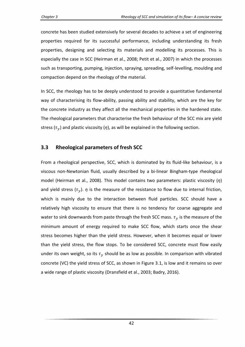
Chapter 3 Rheology of SCC and simulation of its flow– A concise review
42
concrete has been studied extensively for several decades to achieve a set of engineering
properties required for its successful performance, including understanding its fresh
properties, designing and selecting its materials and modelling its processes. This is
especially the case in SCC (Heirman et al., 2008; Petit et al., 2007) in which the processes
such as transporting, pumping, injection, spraying, spreading, self-levelling, moulding and
compaction depend on the rheology of the material.
In SCC, the rheology has to be deeply understood to provide a quantitative fundamental
way of characterising its flow-ability, passing ability and stability, which are the key for
the concrete industry as they affect all the mechanical properties in the hardened state.
The rheological parameters that characterise the fresh behaviour of the SCC mix are yield
stress (𝜏𝑦) and plastic viscosity (η), as will be explained in the following section.
3.3 Rheological parameters of fresh SCC
From a rheological perspective, SCC, which is dominated by its fluid-like behaviour, is a
viscous non-Newtonian fluid, usually described by a bi-linear Bingham-type rheological
model (Heirman et al., 2008). This model contains two parameters: plastic viscosity (η)
and yield stress (𝜏𝑦). η is the measure of the resistance to flow due to internal friction,
which is mainly due to the interaction between fluid particles. SCC should have a
relatively high viscosity to ensure that there is no tendency for coarse aggregate and
water to sink downwards from paste through the fresh SCC mass. 𝜏𝑦 is the measure of the
minimum amount of energy required to make SCC flow, which starts once the shear
stress becomes higher than the yield stress. However, when it becomes equal or lower
than the yield stress, the flow stops. To be considered SCC, concrete must flow easily
under its own weight, so its 𝜏𝑦 should be as low as possible. In comparison with vibrated
concrete (VC) the yield stress of SCC, as shown in Figure 3.1, is low and it remains so over
a wide range of plastic viscosity (Dransfield et al., 2003; Badry, 2016).

Chapter 3 Rheology of SCC and simulation of its flow– A concise review
43
Figure 3.1: Rheology of normal and self-compacting concrete (After: Dransfield et al., 2003)
The potential of a relationship between the SCC rheological characteristics (η and 𝜏𝑦) and
the measured parameters in the slump flow test (namely, slump flow diameter and t500)
has been investigated by many researchers (Thrane et al., 2007; Tregger et al., 2007;
Roussel, 2006a; Kasemchaisiri and Tangtermsirikul, 2008; Zerbino et al., 2009). They
recognised that η is closely related to the time t500 (the higher the η the longer the t500
time) but that the slump flow spread is a function of both the 𝜏𝑦 and the density of SCC.
3.3.1 Measuring the rheological parameters
The relationship between the shear stress and strain rate are routinely measured by an
instrument called rheometer. To obtain the rheological characteristics of general viscous
liquids (such as cement pastes) and solid-liquid suspensions (such as SCCs), a rheometer is
to be used. Several types of this instrument have been proposed to evaluate the η and 𝜏𝑦
of cementitious materials (Ghanbari, 2011). The plastic viscosity of a homogeneous
viscous fluid, such as a paste (mixture of cement, cement replacement material, water
and super–plasticiser) can be measured rather accurately with a viscometer which is not
possible for a non–homogeneous viscous fluid such as an SCC mix. There is a large scatter
in η of one and the same SCC mix measured with different rheometers, as has been
reported by many researchers (Feys et al., 2007; Wallevik and Wallevik, 2011). In this
regard it is also reported (Vasilić, 2015) that ‘‘due to the complexity of the material
behaviour and the concrete rheometer setups, it is nearly impossible to obtain the set of

Chapter 3 Rheology of SCC and simulation of its flow– A concise review
44
actual rheological parameters (plastic viscosity and yield stress) in fundamental units from
rheometer measurements’’. It is therefore necessary to seek alternative methods for
estimating the plastic viscosity of an SCC mix accurately and reliably. Ghanbari and
Karihaloo (2009) have proposed a micromechanical procedure for estimating accurately
the plastic viscosity of an SCC mix knowing the plastic viscosity of the paste used in it. The
description of this procedure will be given in the next chapter (Chapter 4).
As the complex material behaviour disallows the rheological parameters of SCC to be
measured accurately using rheometers, there is a large scatter in the measured yield
stress as there is in the measured plastic viscosity (Vasilić, 2015). It is therefore again
necessary to seek alternative methods for estimating the yield stress of an SCC mix
accurately and reliably. In this regard, numerical simulations could be a tool for
determining this unknown parameter. One such method is to estimate it in an inverse
manner from the measured t500 and flow spread of the mix in a cone flow test using the
three-dimensional smooth particle hydrodynamics (SPH) method for simulating the flow
of SCC (Badry et al., 2016).
3.3.2 Models describing SCC flow
To describe the non-Newtonian flow behaviour of concrete, the two commonly used
models are those of Bingham and Herschel-Bulkley. The Bingham model is the simplest
and most commonly used relation to show the behaviour of a fluid having a 𝜏𝑦. This could
be explained by the fact that this model is most practical: the model parameters can be
measured independently, and the flow of concrete in most cases seems to follow this
relation (Ferraris, 1999). This model is written as:
yy ττττ (3.1)
yττ0 (3.2)
Because SCC can exhibit shear thickening behaviour (Roussel et al., 2010; Heirman et al.,
2009), which means that the plastic viscosity (η) increases with the shear rate ( ), it can
be modelled by the Herschel-Bulkley model (Vasilić et al., 2010). This model is a

Chapter 3 Rheology of SCC and simulation of its flow– A concise review
45
generalisation of the Bingham model in such a way that, upon deformation, the viscosity
can be shear thinning or shear thickening. The constitutive equation in this model is
yy ττττ n (3.3)
yττ0 (3.4)
The fluid exhibits shear thinning, Bingham behaviour and shear thickening behaviour for n
<1, n =1 and n >1, respectively.
3.4 Simulation of SCC flow
Since concrete is put into place in its plastic form, its fresh properties have a direct
influence on the strength and durability in the hardened state (Zerbino et al., 2009). This
is of prime importance in SCC as the prediction of its fresh behaviour is very difficult and
sensitive to the composition and characteristics of its constituents. Although being
verified to satisfy fresh properties by classical experimental tests, SCC may be prone to
defects arising from problems accompanying its production like bleeding, segregation,
incomplete filling, which are particularly problematic when SCC is cast in complex and
heavily reinforced structural members. This could explain the reason why the classical
tests such as slump flow, L-Box, J-ring and V-funnel tests are not always sufficient to fulfil
the SCC self-compactibility criteria and to predict its behaviour. Therefore, performing
numerical simulation of SCC can be a promising aid in overcoming these issues from the
view point of:
➢ providing a useful tool for predicting the SCC rheological parameters (plastic viscosity
and yield stress);
➢ examining whether or not the formwork is completely filled;
➢ investigating the blocking and passing behaviour of the mix as particles migrate
through narrow gaps in reinforcements, especially when large aggregates and/or
fibres are present;

Chapter 3 Rheology of SCC and simulation of its flow– A concise review
46
➢ assisting in proportioning an SCC mix and optimising its ingredients, thus improving
on the traditional trial and error SCC mix design;
➢ investigating the distribution of large aggregates during the flow of concrete and
therefore avoiding segregation and ensuring the homogeneity of the mix;
➢ examining the distribution of fibres and their orientation in the formwork, therefore
optimising the durability and strength of concrete.
3.4.1 Methods for simulating SCC
The simulation methods of concrete flow can be divided into two main groups. First,
methods that treat it as a homogeneous medium in which SCC is regarded as a viscous
fluid without particle inclusions. It is the easiest and fastest way to simulate fresh
concrete. The drawback of this method is that the particle blocking and segregation
cannot be predicted (Roussel, 2007). Second, methods that treat concrete as a
heterogeneous medium in which attention is paid to the differences in the physical
properties between the liquid and granular components used in the concrete and their
effects on the flow. This method highlights the distribution of the large aggregates in this
mix, allowing the actual distribution of coarse aggregates and/or fibres (and their
orientations) to be revealed during the flow. However, selecting the right technique
depends on the purpose of the simulation and whether the solid components of concrete
are considered as separate particles or are embedded in the mortar.
3.4.2 Numerical solution strategy of simulation techniques
In the numerical simulation, there are, in principle, some basic steps as shown in Figure
3.2. In the first step, the focus is on the observed physical phenomenon, which will be
represented by a mathematical model with a set of governing equations. To numerically
solve the governing equations, the next step involves dividing the continuum problem
domain into a discrete number of elements or components. This forms the computational
frame for the numerical approximation which is based on a theory of function

Chapter 3 Rheology of SCC and simulation of its flow– A concise review
47
approximations and includes discrete representation of the governing equations
according to the discretization technique used.
Figure 3.2: The numerical strategy of the simulation technique
3.4.3 The governing equations used in SCC simulation
SCC is represented as a fluid and its flow is governed by the equations of fluid motion: the
continuity, momentum and energy conservation equations which are based on the
fundamental physical laws of conservation. However, when there is no change in the
temperature during a test and the heat flux in the continuum is absent, the energy can be
assumed to be identically conserved. Also, since the viscosity and density are not affected
by the temperature, the energy conservation equation can be omitted.
The continuity equation or the mass conservation equation in the Lagrangian form is
0D
Dt
v (3.5)
Physical phenomenon
Mathematical model
(Governing equations)
Domain discretization
Numerical approximation
(including time step)
Coding

Chapter 3 Rheology of SCC and simulation of its flow– A concise review
48
Here ρ, t, and v are respectively, the fluid particle density, time, and particle velocity. v
is the time rate of change of the volume of a moving fluid element. D denotes the
substantial or material derivative.
For an incompressible fluid, the density is constant, and therefore (3.5) becomes
0 v (3.6)
If gravity (g) is the only body force acting on the continuum, the momentum conservation
equations in the Lagrangian form can be written in the compact vectorial form as
gPDt
D τ
v.
11
(3.7)
where P, g and τ are pressure, gravitational acceleration, and shear stress, respectively.
3.4.4 Fundamental approaches describing the physical governing equations
To describe the physical governing equations, there are two fundamental approaches:
Eulerian and Lagrangian. The Eulerian approach is a spatial description used to track a
certain fixed location in the flow field and follows the change in properties (velocity,
temperature, density, mass, or concentration, etc.) as different fluid elements pass
through that location.
Suppose that the velocity is being followed at a location in the fluid flow through which
different fluid elements pass at different times (Figure 3.3)
11 vt , 22 vt
The time rate of change of the velocity in such a measurement is denoted as z,y,xt
v,
which is the partial derivative of the velocity with respect to time. Note that the suffix (x,
y, z) implies that the observer records the change in the property at the fixed location (x,
y, z).
t
v is also called the local rate of change of that property (velocity in this case).

Chapter 3 Rheology of SCC and simulation of its flow– A concise review
49
Figure 3.3: Different fluid elements at different times at a fixed location in the fluid flow (After: Deeb,
2013)
The Lagrangian approach is used to track a material element of the fluid as it moves and
the changes in its properties, e.g. velocity are monitored. Figure 3.4 illustrates that at
time t1, the ‘material’ or ‘particle’ of the fluid ‘A’ has moved from location (x1, y1, z1) to
another location (x2, y2, z2) at time t2. Its property, say velocity, is recorded, as the
material moves in the flow-field. The recorded property is associated with the same fluid
particle, but at different locations and at different times.
Figure 3.4: Fluid particle motion from time t1 to time t2 (After: Deeb, 2013)
The time change of the velocity in such a measurement is denoted asDt
Dv, which is called
material derivative or substantial derivative. It reflects time rate of change in the velocity
(or any other properties) of the tagged fluid particle as observed by an observer moving
with the fluid. An example of the Lagrangian method is the smooth particle
hydrodynamics (SPH) method.

Chapter 3 Rheology of SCC and simulation of its flow– A concise review
50
The two derivatives, Lagrangian and Eulerian, are related to each other, e.g. for velocity
vvvv
.
tDt
D (3.8)
where the term .v is the convective derivative, which defines the time rate of change as
the fluid element moves from one location to another in the flow field.
3.4.5 Domain Discretization
In the numerical simulations, the continuum problem domain needs to be divided into a
finite number of discrete components in order to numerically solve the governing
equations. This technique is different according to the numerical method used. From a
graphical point of view, computational modelling can be divided into two main
categories, grid and particle-based methods. Figure 3.5 illustrates the two different
discretizations of the same geometrical domain.
Figure 3.5: Comparison between grid method (left) and particle method (right) for the same geometry
(After: Vesenjak and Ren, 2007)
In the grid or mesh-based method, the continuum domain is divided into small discrete
domains connected to each other by nodes. The accuracy of the numerical approximation
is closely related to the mesh topography (i.e. shape, size...etc.). Examples of the mesh-
based method are the finite element method (FEM), the finite difference method (FDM),
and the finite volume method (FVM). Because the generation of the mesh for a grid
method is a prerequisite, for complicated problems it can be more difficult than solving

Chapter 3 Rheology of SCC and simulation of its flow– A concise review
51
the problem itself since the results are based on the quality of the mesh (Vesenjak and
Ren, 2007). Therefore, mesh-less methods become more attractive to treat problems
where it is difficult to use grid based methods.
In particle (or mesh-less) methods, a domain is represented by a set of nodal points or
particles without using any mesh to connect those nodes. In these methods, large
deformations, moving interfaces, difficult boundary conditions and complex geometries
are easy to handle, since the connectivity among nodes is generated as part of the
computation. As an example of mesh-free methods, which will be used for the analysis of
fluid flow in this thesis (Chapter 7), is the smooth particle hydrodynamics (SPH)
(Kulasegaram and Karihaloo, 2013; Deeb et al., 2014a,b).
3.4.6 Numerical approximation- Smooth Particle Hydrodynamics (SPH)
In engineering computational mechanics, mesh-based numerical methods are the primary
computational methodology. However, its efficiency in many complex problems (e.g. free
surface problems, large deformations) is still limited, and therefore the necessity for
developing other computational methods has arisen to avoid the mesh dependency. In
this regard, one of the attractive mesh-free formulations is the Smooth Particle
Hydrodynamics (SPH). It is a Lagrangian particle-based technique for approximating the
continuum fluid through the use of particles. SPH was originally developed to solve
particular astrophysical problems in three-dimensional open space (Lucy, 1977; Gingold
and Monaghan, 1977). Because the motion of SPH particles is similar to liquid or gas flow,
those particles can be simulated using the governing equations of hydrodynamics (Liu and
Liu, 2003).
Thanks to its completely mesh-free nature, with SPH it is easier to model flows with
complex geometry, free surfaces, discontinuity and large deformation. The Lagrangian
nature of SPH allows the grid to be embedded in the material and thus reduces some of
the material interface problems associated with Eulerian techniques. Since it was first
proposed, SPH has gained significant popularity, and with the continuing improvement
and modifications its accuracy, stability and adaptability have reached an acceptable level

Chapter 3 Rheology of SCC and simulation of its flow– A concise review
52
for different engineering applications. In the field of self-compacting concrete (SCC),
which is recognised as a homogeneous fluid that consists of particles of different sizes
and shapes, SPH has been used and proved to be efficient and accurate in simulating the
flow and monitoring the movement of large aggregates and/or short steel fibres (Deeb et
al., 2014a,b,c). It also plays an essential role in the mix proportioning to achieve
appropriate mix ingredients, thereby saving time, effort and materials (Karihaloo and
Ghanbari, 2012; Deeb and Karihaloo, 2013). In addition, SPH provides a useful tool for
predicting the yield stress (𝜏𝑦) of SCC mixes accurately in an inverse manner from the flow
spread (Badry et al., 2016).
3.4.6.1 Key characteristics employed to solve problems in SPH
SPH is an integral interpolation method to approximate values and derivatives of
continuous field quantities by using discrete sample points (Gingold and Monaghan,
1977). As reported by Liu and Liu (2003), the key characteristics employed to solve
problems in SPH are:
SPH support domain: The support domain for a particle, say particle ‘a’, is the domain
where all the information for all particles inside this domain is used to determine the
information at the point ‘a’ (see Figure 3.6). This means that any physical property of a
particle ‘a’ can be obtained by summing the same property of particles that lie in the
support domain Ω within a radius r of the observed particle ‘a’ and multiplying the sum by
a smoothing function W.
Figure 3.6 shows the support domain of particle ‘a’ and all the neighbouring particles ‘b’
that lie in it. Particles which are closer to the centre have a greater contribution to the
property unlike particles outside the influence domain that have no contribution at all,
the influence area of each particle will be therefore defined using the kernel function.
This part is very important in terms of computational effort; for instance, problems with
large deformation that require a huge number of particles could take unacceptably long
CPU time to solve.

Chapter 3 Rheology of SCC and simulation of its flow– A concise review
53
Figure 3.6: Distribution of physical properties of a particle (After: Deeb, 2013)
Kernel approximation: SPH provides a concept to approximate the spatial derivative
using particles, which therefore makes computing the spatial derivatives in particle-based
method as easy as in grid-based methods. Each particle, say particle ‘a’ as illustrated in
Figure 3.6, carries the field variables such as the mass (ma), density (ρa), pressure (Pa),
velocity (va), position (ra), temperature (Ta), colour (ca) and any other quantities
depending on the nature of the flow and of the fluid. The mass is constant through the
simulations. However, the other physical quantities are updated every time step. These
field variables are represented by integral functions, the so-called kernel or smoothing
functions (Figure 3.6).
Particle interpolation: Particle approximation in SPH involves discretising the entire
domain problem into a limited number of particles N, and then approximately calculating
all the field variables on these particles. The finite volume (Vb) of the particle, say particle
‘b’ that lies in the support domain, is calculated as b
bb
mV
, where
b and bm are density
and mass of the particle, respectively. The inclusion of these properties makes SPH the
ideal numerical solution to simulate dynamic fluid flow applications such as the flow of
SCC.

Chapter 3 Rheology of SCC and simulation of its flow– A concise review
54
A quantity xf (Figure 3.7) at an arbitrary position x is approximated using quantities bf
at sample positionsbx . The kernel function W realises a diminishing influence of particles
at larger distances. Over all the particles N in the support domain, xf can be expressed
in the equivalent forms of discretized particle approximation (Bonet and Lok, 1999)
N
b
bbb WfVf1
xxx (3.9)
where xbW is an interpolating kernel, representing the kernel with compact support
domain of radius r (Figure 3.7). There are different possibilities in selecting the kernel
function W. Spline kernel functions are the most common as they can be designed to
have specific characteristics and possess a compact support (Bonet and Kulasegaram,
2000).
The differential of equation (3.9) is given by
N
b
bbb WfVf1
xxx (3.10)
where the quantity xbW denotes the gradient of the kernel, which is taken as centred
on the position of particle a (Figure 3.7).
Figure 3.7: Particle approximation of function f(x) (After: Deeb, 2013)

Chapter 3 Rheology of SCC and simulation of its flow– A concise review
55
Equations (3.9) and (3.10) state that the value of any function (or its differential) at any
position is approximated using the average of the values of the function at all the
particles within the support domain (particles b=1,2,…N) of that particle weighted by the
smoothing function, xbW . The application of equation (3.9) to compute the
approximate value for the density of a continuum leads to the classical SPH equation
N
b
bbWm1
xx (3.11)
3.4.6.2 Boundary conditions
Boundary conditions in SPH should be imposed to ensure balancing the inner particle
forces to prevent those particles from penetrating the wall. To impose boundary
conditions in SPH, different methods are available, such as repulsive forces (Monaghan,
1994), mirror particles (Takeda et al., 1994; Cummins and Rudman, 1999) and dummy
particles (Shao and Lo, 2003; Lee et al., 2008; Amini et al., 2011). In this thesis, the
dummy particle approach will be used as will be explained in Chapter 7.
3.4.6.3 Numerical solution strategies in SPH
In SPH enforcing incompressibility can be pursued using two different approaches - the
truly incompressible SPH (ISPH) (Kulasegaram et al., 2011) and the weakly compressible
SPH (WCSPH) (Monaghan, 1994; Lee et al., 2008). In ISPH approach, a projection method
based on the predictor-corrector time stepping scheme is used to track the flow in which
the SCC incompressibility has been imposed exactly through the pressure Poisson
equation (as will be explained in Chapter 7). In WCSPH approach, the incompressibility
condition is imposed approximately through the so-called weakly or quasi-compressible
SPH (Monaghan, 1994). It leads to the replacement of the real incompressible fluid by an
artificial quasi-compressible fluid having a small, user-defined, fluctuation in the density
in which the time-consuming solution of the Poisson equation can be avoided (Becker and
Teschner, 2007). However, WCSPH requires a much smaller time step in order to keep the
density fluctuation down to 1% to avoid numerical instability (Lee et al., 2008). This can
a

Chapter 3 Rheology of SCC and simulation of its flow– A concise review
56
be circumvented by implementing ISPH (as shown in Chapter 7) in which the pressure and
velocity are computed separately.
3.5 Concluding remarks
In this chapter, the rheology of SCC was introduced, with an overview of the rheological
parameters, the methods of their measurement and the models describing a fluid flow. In
addition to its rheology, the simulation of SCC flow, highlighting the numerical strategy
used in its techniques, was briefly looked at. A review of SPH as a suitable method to
model the SCC flow has also been given briefly in this chapter.
A review of the methods used for measuring the rheological parameters indicates that,
due to the complexity of the material behaviour and the concrete rheometers setups, it is
nearly impossible to obtain these rheological properties reliably from rheometer
measurements. For this reason alternative methods have been developed to determine
these parameters. The yield stress is estimated in an inverse manner from the measured
t500 and flow spread of the mix in a cone flow test using SPH. The plastic viscosity can be
determined using the micromechanical procedure based on the plastic viscosity of the
paste (as will be described in Chapter 4). Here, the micromechanical procedure has not
only been used for determining the SCC plastic viscosity, it also paved the way for
developing a rational mix design method for proportioning SCC mixes. The steps taken to
develop this rational method will be described in Chapter 4.
As we have seen from the reviewed literature, SPH can assist in different areas of SCC
application, such as proportioning SCC mixes, providing a useful tool for predicting the
SCC rheological parameters and modelling the flow and monitoring the movement of
large aggregates and/or short steel fibres in the cone slump flow and L-box tests. Beyond
the scope of its mentioned capabilities, there is another scope for SPH methodology to
simulating SCC mixes in the J-ring test. This will be used to examine whether or not the
produced mixes meet the passing ability criterion and flow homogeneously with no
blockage in complex and heavily reinforced structural members. In Chapter 7 we will
report on the simulation of the flow of fresh SCC in the J-ring test using the SPH approach.

Proportioning of SCC mixes based on target
plastic viscosity and compressive strength:
mix design procedure

Chapter 4 Proportioning of SCC mixes: mix design procedure
58
4.1 Introduction
Self-compacting concrete (SCC) requirements are mostly influenced by the fractions of
the mix ingredients. In other words, to fulfil its main functional requirements (filling
ability, passing ability and segregation resistance), major work in SCC should take into
account designing appropriate volume fractions of the mix ingredients. Without paying
attention to its mix proportioning, SCC will remain to be designed by a number of time
and material-consuming trials before an optimum mix proportion is reached. Although it
has passed from the research phase into real application, methods for proportioning SCC
mixes have not kept pace with their production techniques. This chapter develops a
rational mix design method for SCC based on the desired target plastic viscosity and
compressive strength of the mix. The simplicity and usefulness of this method are
enhanced by the provision of design charts as a guide for mix proportioning. The
characteristic cube strength of these charts varied between 30 and 80 MPa at 28 days
age, and the target plastic viscosity between 3 and 15 Pa s: the upper bound of all mix
grades was 15 Pa s, whereas the lower bound varied between 3 – 8 Pa s in mix grade
range 30 – 80 MPa. Several examples on the use of the design charts are given. In the
next chapter, experimental validation of the mix design procedure is provided on a series
of SCC mixes in both the fresh and hardened states.
The contents of this chapter have been published in the journal ‘Journal of Sustainable
Cement-Based Materials’ (see publication 2 in the list in Chapter 1).
4.2 Exploitation of an idea: mix design development
The proportioning of self-compacting concrete (SCC) mixes requires a balance between
their flow and passing ability on the one hand and the resistance to segregation on the
other (Corinaldesi and Moriconi, 2004; Wu and An, 2014; Okamura and Ouchi, 2003). The
early mix proportioning approaches proposed by Okumara and Ouchi (1999) and
Domone (2000) and later developed by others (Okamura et al., 2000) were all heuristic in
nature requiring many trial mixes. However, the extensive research work carried out on
the rheological properties of SCC (Roussel, 2006b; Tregger et al., 2012; Saak et al., 2001;

Chapter 4 Proportioning of SCC mixes: mix design procedure
59
Chidiac and Mahmoodzadeh, 2009; Figueiras et al., 2014; Wallevik and Wallevik, 2011;
Petersson and Billberg, 1999; Li and Kwan, 2011; Li and Kwan, 2013) has greatly improved
the proportioning of SCC mixes. A summary of different mix proportioning approaches
can be found in Shi et al. (2015). The European Federation of National Trade Associations
(EFNARC) guidelines (EFNARC, 2005) give typical ranges of primary ingredients; the actual
amounts depend on the desired strength and other performance requirements. Thus the
mix proportioning still involves considerable trial and error.
A rigorous method for proportioning normal and high strength SCC mixes based on their
plastic viscosity has been proposed in (Karihaloo and Ghanbari, 2012 and Deeb and
Karihaloo, 2013). It exploits the expression for the plastic viscosity of an SCC mix
developed by Ghanbari and Karihaloo (2009) using micro-mechanical principles. This
expression shows how the known plastic viscosity of the paste is increased by the
addition of solid phase particles, i.e. filler, fine and coarse aggregates. The contribution of
each of the solid phases to the overall increase depends on its volume fraction and shape
of its particles. As a result, the final expression for the plastic viscosity of an SCC mix is the
product of the known plastic viscosity of the paste and contributions of each of the solid
phases.
While the method proposed in (Karihaloo and Ghanbari, 2012 and Deeb and Karihaloo,
2013) is rigorous and based on sound physical principles, it produces a bewildering array
of mixes that reach the target plastic viscosity but does not give any practical guidelines
on how to choose the most appropriate mix. Moreover, the method was developed on
the basis of reference mixes of a range of known cube compressive strength, but the
latter was not explicitly imposed as a design criterion.
This chapter will overcome the above shortcomings of this method for proportioning SCC
mixes. Practical guidelines in the form of design charts will be provided for choosing the
mix proportions that achieve the target compressive strength and the target plastic
viscosity.

Chapter 4 Proportioning of SCC mixes: mix design procedure
60
4.3 Target compressive strength
The compressive strength of a concrete mix is mostly determined by the ratio of water to
cementitious material (w/cm) under given curing conditions. A regression analysis was
performed on the data collected from many published sources (Deeb and Karihaloo,
2013; Beygi et al., 2013a,b; Dinakar et al., 2013a,b; Panesar and Shindman, 2011;
Felekoǧlu et al., 2007; Rozière et al., 2007; Nikbin et al., 2014a,b; Boukendakdji et al.,
2012; Persson, 2001; Leemann and Hoffmann, 2005; Parra et al., 2011; Nuruddin et al.,
2014; Zhu and Gibbs, 2005; Carpinteri and Brighenti, 2010; Rabehi et al., 2013; Beygi et
al., 2014a; Dinakar et al., 2008; Collepardi et al., 2007; Khaloo et al., 2014; Bui et al., 2002;
Domone, 2007; Ferrara et al., 2007) and on the data obtained in various studies in Cardiff
University (Figure 4.1). It was found that the compressive strength of SCC (MPa) could be
best fitted by an Abrams-type relation (R2 =0.94):
𝑓𝑐𝑢 =195
12.65(𝑤/𝑐𝑚) (4.1)
where 𝑓𝑐𝑢 is the 28-day equivalent cube compressive strength (MPa) and w/cm is the
ratio of water to cementitious materials (i.e. cement + cement replacement material, e.g.
ggbs). The large scatter in the surveyed data is no doubt a reflection of the differences in
the curing conditions, the cement type, the type of cement replacement material and
replacement levels up to 30% and the amount and the maximum size of coarse aggregate.
The values have been adjusted for the size of the cube test specimens to that of 100 mm
cubes. It was found however (see later) that formula (4.1) overestimates the cube
compressive strength of low strength (30 – 40 MPa) SCC mixes. This is perhaps a result of
the presence of high powder content in these mixes, as has also been stated in
(Nanthagopalan and Santhanam, 2009). For 30 MPa mix, the w/cm predicted by (4.1)
needs to be decreased by approximately 14% and that for 40 MPa mix by 8%.

Chapter 4 Proportioning of SCC mixes: mix design procedure
61
Figure 4.1: Relation between compressive strength and water to cementitious material ratio
4.4 Target plastic viscosity
Fresh SCC is a non–Newtonian fluid best described by a Bingham–type model. This model
contains two rheological parameters of SCC, namely its yield stress and plastic viscosity
(Dransfield, 2003). It is known however, that the yield stress of SCC mixes is low (in the
order of tens of Pa) in comparison with vibrated concrete mixes and it remains so over a
wide range of plastic viscosity (Dransfield, 2003; Badry, 2016). Thus the most important
parameter is the plastic viscosity which changes with the plastic viscosity of the paste and
the mix composition.
R² = 0.9366
20
30
40
50
60
70
80
90
100
110
120
0.2 0.3 0.4 0.5 0.6 0.7 0.8
f cu
, M
Pa
w/cm
Deeb and Karihaloo (2013)Beygi et al. (2013a)Dinakar et al. (2013a)Panesar and Shindman (2011) Felekoğlu et al. (2007)Rozie`re et al. (2007)Nikbin et al. (2014a)Boukendakdji et al. (2012)Persson (2001)Dinakar et al. (2013b)Leemann and Hoffmann (2005)Parra et al. (2011)Beygi et al. (2013b)Nuruddin et al. (2014)Zhu and Gibbs (2005)Carpinteri and Brighenti (2010)Rabehi et al. (2013)Beygi et al. (2014a)Dinakar et al. (2008)Collepardi et al. (2007)Nikbin et al. (2014b)Khaloo et al. (2014)Bui et al. (2002)Domone (2007)Ferrara et al. (2007)Cardiff test 1Cardiff test 2Cardiff test 3Cardiff test 4Cardiff test 5Cardiff test 6Cardiff test 7Cardiff test 8Cardiff test 9

Chapter 4 Proportioning of SCC mixes: mix design procedure
62
The plastic viscosity of a homogeneous viscous fluid, such as a paste (mixture of cement,
cement replacement material, water and super-plasticiser) can be measured rather
accurately with a viscometer which is not possible for a non-homogenous viscous fluid
such as an SCC mix. There is a large scatter in the plastic viscosity of the same SCC mix
measured with different rheometers, as has been noticed by many researchers (Wallevik
and Wallevik, 2011; Banfill et al., 2000; Feys et al., 2007). Ghanbari and Karihaloo (2009)
have therefore proposed a micromechanical procedure for estimating the plastic viscosity
of an SCC mix knowing the plastic viscosity of the paste used in it. In this procedure, SCC is
regarded as a two–phase suspension in which the solid phase is suspended in a viscous
liquid phase. The increase in the plastic viscosity of the liquid phase as a result of the
addition of the solid phase (filler, fine and coarse aggregates) is estimated in a stepwise
manner from the two-phase suspension model. In the first step, the solid phase is the
finest solid material, for example the filler in the viscous fluid phase i.e. the paste. In the
next step, the finest solid i.e. fine aggregate is the solid phase suspended in the viscous
fluid phase now formed by the two-phase suspension from the first step. This procedure
is continued until all the solid phase ingredients have been added. The plastic viscosity of
the i–th liquid-solid suspension can be estimated from the plastic viscosity of the
preceding (i–1)th phase as
𝜂𝑐𝑖 = 𝜂𝑐𝑖−1×𝑓𝑖(𝜙𝑖) (4.2)
Here,
𝜂𝑐𝑖 = plastic viscosity of the i–th liquid–solid suspension; 𝜂𝑐𝑖−1 = plastic viscosity of the
preceding (i–1)th phase. In the first step i = 1, 𝜂𝑐0 is the known plastic viscosity of the
paste; 𝑓𝑖(𝜙𝑖) = a factor larger than unity that predicts the increase in the plastic viscosity
induced the solid phase with a volume fraction 𝜙𝑖. Figure 4.2 shows the hierarchy of
these two-phase (liquid-solid) suspensions used in the estimation of the plastic viscosity
of all mixes developed based on the viscosity of the cement paste used in them.

Chapter 4 Proportioning of SCC mixes: mix design procedure
63
Figure 4.2: Hierarchy of two-phase liquid-solid suspensions constituting an SCC mix
According to this procedure, the plastic viscosity of an SCC mix is given by:
𝜂𝑚𝑖𝑥 = 𝜂𝑝𝑎𝑠𝑡𝑒×𝑓1(𝜙1)×𝑓2(𝜙2)…×𝑓𝑛(𝜙𝑛) (4.3)
where 𝑛 is the total number of solid phases in the mix. Besides the filler, fine and coarse
aggregates, air voids can also be treated as a second phase in a viscous suspension.
Einstein was the first to develop an expression 𝑓𝑖(𝜙𝑖) for dilute suspensions (second
phase volume fraction less than 10%) containing randomly distributed rigid or hollow
spheres with no hydrodynamic interactions (Koehler and Fowler, 2007):
𝑓𝑖(𝜙𝑖) = 1 + [𝜂]𝜙𝑖 (4.4)
The numerical factor [𝜂] is equal to 2.5 for rigid spherical particles and to 1 for spherical
air bubbles that are packed randomly in a hexagonal arrangement. Subsequent
investigations have proved that the numerical factor 2.5 is quite accurate even for rigid
ellipsoidal particles with an aspect ratio less than 3.
However, at higher concentrations of the solid phase (volume fraction >10% up to the
maximum possible volume fraction, 𝜙𝑚), the hydrodynamic interactions between the
particles and the Brownian motions cannot be ignored. In this situation, the Krieger–
Dougherty (Krieger, 1959) formula (Eq. (4.5)) has been found to be appropriate for
cement–based suspensions. The value of 𝜙𝑚 is 0.74 for hexagonal close packing, 0.63 for
random hexagonal packing, and 0.524 for cubic packing
𝑓𝑖(𝜙𝑖) = (1 −𝜙𝑖
𝜙𝑚)−[𝜂]𝜙𝑚 (4.5)
Air
Paste
Filler
Paste + Air
Paste + Air
+ Filler
Paste + Air +
Filler + Fine
aggregate
Coarse aggregate
Fine aggregate

Chapter 4 Proportioning of SCC mixes: mix design procedure
64
The particle size distribution significantly affects 𝜙𝑚. Furthermore, the numerical factor
[𝜂] and 𝜙𝑚 depend upon the shear rate; the former tends to decrease with increasing
shear rate, whereas the latter shows the opposite trend. However, [𝜂] and 𝜙𝑚 change in
such a way that a decrease in the first leads to an increase in the second, but the product
of both changes remains practically the same and equal, on average, to 1.9 (de Kruif et
al., 1985). In most SCC mixes, the volume fractions of the filler, fine and coarse aggregates
generally exceed 10%, so that their contribution to the increase in the known plastic
viscosity of the paste is given by Eq. (4.5). The volume fraction of the trapped air bubbles
is however low, around 2%, such that Eq. (4.4) with the numerical factor equal to 1 is
appropriate. For simplicity, this 2% increase due to trapped air is included in the plastic
viscosity of the paste in Eq. (4.6):
𝜂𝑚𝑖𝑥 = 𝜂𝑝𝑎𝑠𝑡𝑒× (1 −𝜙𝐹𝑖𝑙𝑙𝑒𝑟
𝜙𝑚)−1.9
× (1 −𝜙𝐹𝑖𝑛𝑒 𝐴𝑔𝑔.
𝜙𝑚)−1.9
× (1 −𝜙𝐶𝑜𝑎𝑟𝑠𝑒 𝐴𝑔𝑔.
𝜙𝑚)−1.9
(4.6)
Note that the packing density (i.e. the maximum volume fraction, 𝜙𝑚) increases with the
addition of solid phases. When the first solid phase is added to the paste, the packing is
loose so that it is appropriate to assume cubic packing. When however, the last solid
phase is added to the suspension, the packing is very dense and it is appropriate to
assume hexagonal close packing.
4.5 Calculating the plastic viscosity of SCC mixes
The calculation of the plastic viscosity will be demonstrated on a mix 40A (as it is designed
in Chapter 5) as an example and it is the same procedure for all developed SCC mixes.
Step 1: Estimating the plastic viscosity of the liquid phase(𝜼𝐩𝐚𝐬𝐭𝐞).
The plastic viscosity of the cement paste (cement + ggbs + SP + water + air) is estimated
by using the literature (Sun et al., 2006; Nehdi and Rahman, 2004) and it equals to 0.18 Pa
s (see Table 4.1).

Chapter 4 Proportioning of SCC mixes: mix design procedure
65
Table 4.1: Estimated plastic viscosity of the paste (cement +ggbs + SP+ water+ air)
w/cm 𝜼𝒑𝒂𝒔𝒕𝒆 , Pa s 𝜼𝒑𝒂𝒔𝒕𝒆+𝒂𝒊𝒓 𝒗𝒐𝒊𝒅𝒔, Pa s
0.63 0.104 0.11
0.57 0.176 0.18
0.53 0.224 0.23
0.47 0.286 0.29
0.40 0.330 0.34
0.35 0.365 0.37
Step 2: Adding the first solid phase i.e. limestone powder (LP)
In this case, limestone powder (LP) is considered the solid phase and cement paste
(cement + ggbs + SP + water + air) is the liquid phase. The volume fraction of the solid
phase is determined using Eq. (4.7):
( 𝜙𝐿𝑃 =𝑣𝐿𝑃
𝑣𝐿𝑃+𝑣𝑝 ) (4.7)
Here, 𝑣𝐿𝑃: is the volume fraction of the solid phase (limestone powder), 𝑣𝑝: is the volume
of the continuous matrix phase (paste volume) in which the solid phase is suspended.
After calculating the volume of each ingredient in the mix, the volume of paste is 𝑣𝑝 =
0.346 m3, limestone powder is considered the solid phase and the components within the
container are the liquid phase. The volume fraction of LP is:
𝜙𝐿𝑃 =0.041
0.041+0.346= 0.106 > 0.10
Using Eq. (4.5); ([𝜂]×𝜙𝑚) = -1.9 and 𝜙𝑚= 0.524, gives;
𝑓𝐿𝑃(𝜙𝐿𝑃) = (1 −0.106
0.524)−1.9
= 1.536
Based on Eq. (4.2); the plastic viscosity of the suspension is:
𝜂(𝜙𝐿𝑃+𝑎𝑖𝑟+𝑝) = 𝜂𝑝𝑎𝑠𝑡𝑒×𝑓𝐿𝑃(𝜙𝐿𝑃) = 0.18×1.536 = 0.276 Pa s

Chapter 4 Proportioning of SCC mixes: mix design procedure
66
Step 3: Adding the fine aggregate (FA)
Fine aggregate (FA) is now considered as the solid phase and the ingredients in the
container as the liquid phase. The volume fraction of FA is
𝜙𝐹𝐴 = 0.420 > 0.10
Using Eq. (4.5); ([𝜂]×𝜙𝑚) = -1.9 and 𝜙𝑚= 0.63, gives;
𝑓𝐹𝐴(𝜙𝐹𝐴) = (1 −0.420
0.630)−1.9
= 8.064
Based on Eq. (4.2); the plastic viscosity of the mix so far is:
𝜂(𝜙𝐹𝐴+𝐿𝑃+𝑎𝑖𝑟+𝑝) = 𝜂𝑝𝑎𝑠𝑡𝑒×𝑓𝐿𝑃(𝜙𝐿𝑃)×𝑓𝐹𝐴(𝜙𝐹𝐴)
= 0.18×1.536×8.064 = 2.230 Pa s
Step 4: Adding the coarse aggregates (CA)
Coarse aggregates are now considered as the solid phase and the ingredients in the
container as the liquid phase. The volume fraction of CA is
𝜙𝐶𝐴 = 0.330 > 0.10
Using Eq. (4.5); ([𝜂]×𝜙𝑚) = -1.9 and 𝜙𝑚= 0.74, gives;
𝑓𝐶𝐴(𝜙𝐶𝐴) = (1 −0.330
0.740)−1.9 = 3.071
Based on Eq. (4.2); the plastic viscosity of the final mix is:
𝜂(𝜙𝐶𝐴+𝐹𝐴+𝐿𝑃+𝑎𝑖𝑟+𝑝) = 𝜂𝑝𝑎𝑠𝑡𝑒×𝑓𝐿𝑃(𝜙𝐿𝑃)×𝑓𝐹𝐴(𝜙𝐹𝐴)×𝑓𝐶𝐴(𝜙𝐶𝐴)
= 0.18×1.536×8.064×3.071 = 6.847Pa s
The results of the plastic viscosity calculation of mix 40A are summarised in Table 4.2.

Chapter 4 Proportioning of SCC mixes: mix design procedure
67
Table 4.2: Summarising the results of the plastic viscosity calculation of mix 40A
Ingredients Mass, kg/m3 Volume, m3 𝜙 f(𝜙)
Paste – 0.346 – –
Limestone powder 100 0.041 0.106 1.536
Fine Aggregate 748 0.282 0.420 8.064
Coarse Aggregate 924 0.330 0.330 3.071
4.6 Basic steps of the proposed mix design method
The basic steps of the proposed mix design method are summarised below.
1. Select the desired plastic viscosity of the mix within the range of 3–15 Pa s,
remembering that the slump cone t500 time increases with increasing plastic viscosity
of the mix. EFNARC (2005) will be helpful in the choice of the desired plastic viscosity
depending on the application;
2. Calculate the ratio of water to cementitious materials (w/cm) that produces the target
cube characteristic strength from Eq. (4.1);
3. Choose the water content in the range of 150–210 kg/m3, following EFNARC (2005),
and calculate the mass of cementitious materials (cm) in kg/m3. The amount of ggbs is
assumed to be 25% of cementitious material (cm). It is known (Nehdi and Rahman,
2004) that the replacement of 25% cement (c) by ggbs has little or no effect on the
paste viscosity;
4. Assume a trial super-plasticiser (SP) dosage as a per cent of the cementitious material
mass in the range of 0.4–0.8 % for the MasterGlenium super-plasticiser used in this
work. For this super-plasticiser the manufacturer’s recommended dosage is 0.2 – 1.2
kg per 100 kg of cementitious material (BASF, 2014).
5. Estimate the plastic viscosity of the paste from the w/cm and SP/cm ratios (Sun et al.,
2006; Nehdi and Rahman, 2004) (see Table 4.1). It is known that SP/cm has little
impact on the paste viscosity; the major impact is on the yield stress (Domone, 2003);

Chapter 4 Proportioning of SCC mixes: mix design procedure
68
6. Calculate the mass of the solid phase ingredients (filler, fine aggregate and coarse
aggregate) according to their volume fractions, as explained in the examples below;
7. Check if the total volume of the produced mix is equal to 1.0 m3. If not, scale the
ingredient masses to achieve a total volume of 1.0 m3;
8. Calculate the plastic viscosity of the mix using Eq. (4.6) and compare it with the desired
one (step 1). If the difference is within ±5%, adopt the mix proportions. If not, choose a
different combination of the volume fractions of the solid phase ingredients (step 6)
and repeat steps 7–8.
The steps of the proposed mix design method are shown in the flow-chart below (Figure
4.3).

Chapter 4 Proportioning of SCC mixes: mix design procedure
69
Figure 4.3: Flow-chart of the proposed mix design method
Calculate w/cm according to selected fcu
Choose water content (150-210) l/m3
Calculate the cm content and assume SP dosage
𝑡1×𝑡2×𝑡3
= 1.0
Select target viscosity, 𝜂𝑚𝑖𝑥
Calculate paste viscosity, 𝜂𝑝𝑎𝑠𝑡𝑒
Select the arbitrary factors 𝑡1, 𝑡2, and 𝑡3
No
No
No
Scale the masses to achieve 1.0 m3
Calculate 𝜂𝑚𝑖𝑥 and check within
±5% of the target
Yes
Yes
Adopt the mix as SCC
Calculate ingredient volume fractions, 𝜙𝐿𝑃, 𝜙FA and 𝜙CA
Calculate ingredient masses, LP, FA and CA
Total volume = 1.0 m3
Yes

Chapter 4 Proportioning of SCC mixes: mix design procedure
70
4.7 Examples of mix proportioning
As an example, let us proportion the mix of an SCC having a 28-day target cube
compressive strength of 50 MPa. The procedure is as follows:
1. Suppose that the desired target plastic viscosity of the mix is equal to 7 Pa s;
2. Calculate the w/cm ratio from Eq. (4.1) corresponding to strength grade C50. It works
out to be 0.53;
3. Assume the water content, 𝑤 to be 200 kg/m3, then the mass of cementitious
materials (cm);
𝑐𝑚 = 𝑤
(𝑤/𝑐𝑚)=
200
0.53= 377.4 kg/m3;
4. Assume a trial SP dosage as a per cent of mass of cementitious materials (say 0.65%)
which equals 2.45 kg/m3 ;
5. Estimate the plastic viscosity of the paste; 𝜂𝑝𝑎𝑠𝑡𝑒 = 0.23 Pa s (Table 4.1);
6. In order to estimate the volume fractions of filler (LP), fine aggregate (FA) and coarse
aggregate (CA), we first rewrite Eq. (4.6) as (note the use of different packing
densities, as explained above);
𝜂𝑚𝑖𝑥 = 𝜂𝑝𝑎𝑠𝑡𝑒×(1 −𝜙𝐿𝑃0.524
)−1.9
× (1 −𝜙𝐹𝐴0.63
)−1.9
× (1 −𝜙𝐶𝐴0.74
)−1.9
Let 𝑢 = (𝜂𝑚𝑖𝑥
𝜂𝑝𝑎𝑠𝑡𝑒×0.524−1.9×0.63−1.9×0.74−1.9)
1
−1.9
so that the above equation becomes 𝑢= (0.524−𝜙𝐿𝑃) × (0.63−𝜙𝐹𝐴) × (0.74−𝜙𝐶𝐴)
Substituting 𝜂𝑚𝑖𝑥 = 7 Pa s and 𝜂𝑝𝑎𝑠𝑡𝑒 = 0.23 Pa s, gives
𝑢 = 0.0405 = (0.524−𝜙𝐿𝑃) × (0.63−𝜙𝐹𝐴) × (0.74−𝜙𝐶𝐴)
Let 𝑥 = √u 3
= 0.343,
then the values of 𝜙𝐿𝑃, 𝜙𝐹𝐴 and 𝜙𝐶𝐴 are given by
𝜙𝐿𝑃= 0.524−𝑡1×𝑥 , 𝜙𝐹𝐴= 0.63−𝑡2×𝑥 , 𝜙𝐶𝐴= 0.74−𝑡3×𝑥

Chapter 4 Proportioning of SCC mixes: mix design procedure
71
where, 𝑡1, 𝑡2, and 𝑡3 are arbitrarily chosen factors such that 𝑡1×𝑡2×𝑡3 = 1.0 Let us choose
𝑡1 = 1.0, 𝑡2 = 1.0 and 𝑡3= 1.0, in the first instance.
For this choice of t1, t2, and t3, the volume fractions of solid phases will be
𝜙𝐿𝑃= 0.524−𝑡1×𝑥= 0.524–1×0.343= 0.181
𝜙𝐹𝐴= 0.63−𝑡2×𝑥= 0.63–1×0.343= 0.287
𝜙𝐶𝐴= 0.74−𝑡3×𝑥= 0.74–1×0.343= 0.397
The amounts of solid phases, i.e. limestone filler (LP), fine aggregate (FA) and coarse
aggregate (CA) that are suspended in the liquid paste are calculated according to their
volume fractions (𝜙𝑖), knowing that the densities of cement, ggbs, water, super-
plasticiser, limestone powder, fine aggregate and coarse aggregate are 2950, 2400, 1000,
1070, 2400, 2650 and 2800 kg/m3, respectively:
𝜙𝐿𝑃 =
𝐿𝑃
𝜌𝐿𝑃
(𝑐
𝜌𝑐+𝑔𝑔𝑏𝑠
𝜌𝑔𝑔𝑏𝑠+𝑤
𝜌𝑤+𝑆𝑃
𝜌𝑆𝑃+0.02)+
𝐿𝑃
𝜌𝐿𝑃
→ LP = 189 kg/m3
𝜙𝐹𝐴 =
𝐹𝐴
𝜌𝐹𝐴
(𝑐
𝜌𝑐+𝑔𝑔𝑏𝑠
𝜌𝑔𝑔𝑏𝑠+𝑤
𝜌𝑤+𝑆𝑃
𝜌𝑆𝑃+𝐿𝑃
𝜌𝐿𝑃+0.02)+
𝐹𝐴
𝜌𝐹𝐴
→ FA = 465 kg/m3
𝜙𝐶𝐴 =
𝐶𝐴
𝜌𝐶𝐴
(𝑐
𝜌𝑐+𝑔𝑔𝑏𝑠
𝜌𝑔𝑔𝑏𝑠+𝑤
𝜌𝑤+𝑆𝑃
𝜌𝑆𝑃+𝐿𝑃
𝜌𝐿𝑃+𝐹𝐴
𝜌𝐹𝐴+0.02)+
𝐶𝐴
𝜌𝐶𝐴
→ CA = 1126 kg/m3
7. The total volume of the SCC mix that the above ingredients will yield (including the
volume occupied by trapped air bubbles, 0.02)
Total Vol. =𝑐
𝜌𝑐+
𝑔𝑔𝑏𝑠
𝜌𝑔𝑔𝑏𝑠+
𝑤
𝜌𝑤+
𝑆𝑃
𝜌𝑆𝑃+
𝐿𝑃
𝜌𝐿𝑃+
𝐹𝐴
𝜌𝐹𝐴+
𝐶𝐴
𝜌𝐶𝐴+ 0.02
Total Vol. =377.4×0.75
2950+377.4×0.25
2400+
200
1000+
2.45
1070+
189
2400+
465
2650+1126
2800+ 0.02 =
1.014 m3
As the yield does not equal 1.0 m3, the amounts of materials are adjusted, and the mix
plastic viscosity is recalculated using Eq. (4.6).

Chapter 4 Proportioning of SCC mixes: mix design procedure
72
cm= 377.4/1.014= 372.2 kg/m3
w=200/1.014= 197.2 kg/m3
SP= 2.45/1.014= 2.42 kg/m3
LP= 189/1.014= 186 kg/m3
FA= 465/1.014= 459 kg/m3
CA= 1126/1.014= 1110 kg/m3
Total Vol. =𝑐
𝜌𝑐+
𝑔𝑔𝑏𝑠
𝜌𝑔𝑔𝑏𝑠+
𝑤
𝜌𝑤+
𝑆𝑃
𝜌𝑆𝑃+
𝐿𝑃
𝜌𝐿𝑃+
𝐹𝐴
𝜌𝐹𝐴+
𝐶𝐴
𝜌𝐶𝐴+ 0.02 = 1.0 m3
8. The mix plastic viscosity is calculated by using Eq. (4.6). As the difference between the
target plastic viscosity and the actual mix plastic viscosity is within ±5%, the mix
proportions after adjustment are acceptable. The mix masses before and after scaling
to 1.0 m3 are given in Table 4.3.
Table 4.3: Mix constituents and plastic viscosity of an SCC mix
Ingredient, kg/m3
𝜼, Pa s Difference cement ggbs w SP LP FA CA
Before adjust. 283 94 200 2.45 189 465 1126 –
0.6% After adjust. 279 93 197 2.42 186 459 1110 7.04
Density 2950 2400 1000 1070 2400 2650 2800 –
However, the amount of coarse aggregate exceeds the limit in the guidelines (EFNARC,
2005), so it is necessary to reduce it and to adjust the mix proportions by choosing
different arbitrary values of 𝑡1, 𝑡2 and 𝑡3 for the same target plastic viscosity and strength:
Steps 1-5 are the same as described above.

Chapter 4 Proportioning of SCC mixes: mix design procedure
73
6. In order to calculate the volume fractions of solid phases, let choose values of t1, t2,
and t3 different from those used above. Let 𝑡1 = 1.1, 𝑡2 = 0.7 and 𝑡3 = 1.3 such
that 𝑡1×𝑡2×𝑡3 = 1.0. Accordingly, the volume fractions of solid phases work out to be
𝜙𝐿𝑃 = 0.147, 𝜙𝐹𝐴 = 0.390 and 𝜙C𝐴 = 0.294. The amounts of solid phases, i.e. limestone
filler (LP), fine aggregate (FA) and coarse aggregate (CA) that are suspended in the
liquid paste are calculated according to their volume fractions (𝜙𝑖);
𝜙𝐿𝑃 =
𝐿𝑃
𝜌𝐿𝑃
(𝑐
𝜌𝑐+𝑔𝑔𝑏𝑠
𝜌𝑔𝑔𝑏𝑠+𝑤
𝜌𝑤+𝑆𝑃
𝜌𝑆𝑃+0.02)+
𝐿𝑃
𝜌𝐿𝑃
→ LP = 147 kg/m3
𝜙𝐹𝐴 =
𝐹𝐴
𝜌𝐹𝐴
(𝑐
𝜌𝑐+𝑔𝑔𝑏𝑠
𝜌𝑔𝑔𝑏𝑠+𝑤
𝜌𝑤+𝑆𝑃
𝜌𝑆𝑃+𝐿𝑃
𝜌𝐿𝑃+0.02)+
𝐹𝐴
𝜌𝐹𝐴
→ FA = 707 kg/m3
𝜙𝐶𝐴 =
𝐶𝐴
𝜌𝐶𝐴
(𝑐
𝜌𝑐+𝑔𝑔𝑏𝑠
𝜌𝑔𝑔𝑏𝑠+𝑤
𝜌𝑤+𝑆𝑃
𝜌𝑆𝑃+𝐿𝑃
𝜌𝐿𝑃+𝐹𝐴
𝜌𝐹𝐴+0.02)+
𝐶𝐴
𝜌𝐶𝐴
→ CA = 799 kg/m3
7. The total volume of the SCC mix that the above ingredients will yield (including the
volume occupied by trapped air bubbles, 0.02);
Total Vol. =𝑐
𝜌𝑐+
𝑔𝑔𝑏𝑠
𝜌𝑔𝑔𝑏𝑠+
𝑤
𝜌𝑤+
𝑆𝑃
𝜌𝑆𝑃+
𝐿𝑃
𝜌𝐿𝑃+
𝐹𝐴
𝜌𝐹𝐴+
𝐶𝐴
𝜌𝐶𝐴+ 0.02 = 0.972 m3
As the yield does not equal to 1.0 m3, the amounts of ingredients are adjusted. The
results are shown in Table 4.4.
8. The mix plastic viscosity is calculated by using Eq. (4.6). As the difference between the
target plastic viscosity and the actual mix plastic viscosity is within ±5%, the mix
proportions after adjustment are acceptable.

Chapter 4 Proportioning of SCC mixes: mix design procedure
74
Table 4.4: Mix constituents and plastic viscosity of an SCC mix
Ingredient, kg/m3
𝜼, Pa s Difference cement ggbs w SP LP FA CA
Before adjust. 283 94 200 2.45 147 707 799 –
0.3 % After adjust. 291 97 206 2.52 151 727 822 7.02
Density 2950 2400 1000 1070 2400 2650 2800 –
In view of the arbitrariness in the choice of 𝑡𝑖, it is clear that there are many (theoretically
infinite) combinations of the volume fractions of the solid phases that can be chosen for
an SCC mix and still reach the target cube compressive strength and mix plastic viscosity.
It is however possible that some of these combinations may not yield a satisfactory SCC
mix. It is therefore necessary to use other sources of information based on accumulated
knowledge of SCC mixes, e.g. the EFNARC (2005) and survey report (Domone, 2006), as
was done above. To aid the user in making a knowledgeable choice, a software program
(Appendix A) was developed from which design charts were constructed which are
presented below.
4.8 Design charts for mix proportioning of normal and high strength SCC
mixes
Thousands of solid phase volume fraction combinations (i.e. t1, t2, and t3) were produced
using a software program. These combinations covered wide ranges of target cube
compressive strength and mix plastic viscosity. They have been collected in groups
according to the target strength for ease of SCC mix proportioning. It was found
convenient for presentation of a huge body of data to normalise the amounts of dry
phases by the plastic viscosity and to present the amounts in separate plots, beginning
with the cementitious materials (cm), and ending with the content of all dry phases (cm +
LP + FA + CA). These design charts are given in Figures 4.4–4.9. The scatter reflects the
multiplicity of combinations. It is however interesting to note that the scatter is the least
in the bottom (cm) and the top (cm + LP + FA + CA) curves. This is because the amount of

Chapter 4 Proportioning of SCC mixes: mix design procedure
75
cm calculated from the target compressive strength is according to the water content
which varies in the narrow range of 150-210 l/m3 (EFNARC, 2005) and the amounts of all
dry ingredients contribute to the target plastic viscosity of the mix.
Moreover, it should be mentioned that the target plastic viscosity of the constructed
design charts varies between 3 and 15 Pa s: the upper bound of all mix grades is 15 Pa s,
whereas the lower bound varies between 3 – 8 Pa s for the mix grades 30 – 80 MPa,
respectively. This is because some of the SCC mix parameters and fresh flow
characteristics (cement replacement level, water content, super-plasticiser dosage and
flow spread) have been chosen within certain restricted limits. For example, the
replacement level of cement by ggbs was only allowed up to 25%, the target flow spread
was restricted to the range of 700±50 mm, the water content was allowed to vary
between 150 and 210 l/m3 and the SP dosage was in the range of 0.4–0.8 % as a per cent
of the mass of the cementitious material (cement + ggbs).

Chapter 4 Proportioning of SCC mixes: mix design procedure
76
Figure 4.4: Ingredient mass (kg) normalised by mix plastic viscosity vs plastic viscosity for 30 MPa mix
(cm+LP+FA+CA)/η
(cm+LP+FA)/η
cm/η
(cm+LP)/η

Chapter 4 Proportioning of SCC mixes: mix design procedure
77
Figure 4.5: Ingredient mass (kg) normalised by mix plastic viscosity vs plastic viscosity for 40 MPa mix
cm/η
(cm+LP)/η
(cm+LP+FA)/η
(cm+LP+FA+CA)/η

Chapter 4 Proportioning of SCC mixes: mix design procedure
78
Figure 4.6: Ingredient mass (kg) normalised by mix plastic viscosity vs plastic viscosity for 50 MPa mix
(cm+LP+FA)/η
(cm+LP)/η
cm/η
(cm+LP+FA+CA)/η

Chapter 4 Proportioning of SCC mixes: mix design procedure
79
Figure 4.7: Ingredient mass (kg) normalised by mix plastic viscosity vs plastic viscosity for 60 MPa mix

Chapter 4 Proportioning of SCC mixes: mix design procedure
80
Figure 4.8: Ingredient mass (kg) normalised by mix plastic viscosity vs plastic viscosity for 70 MPa mix
(cm+LP+FA+CA)/η
(cm+LP+FA)/η
(cm+LP)/η
cm/η

Chapter 4 Proportioning of SCC mixes: mix design procedure
81
Figure 4.9: Ingredient mass (kg) normalised by mix plastic viscosity vs plastic viscosity for 80 MPa mix
R² = 0.9961
R² = 0.9744
R² = 0.9561
R² = 0.9994
0
20
40
60
80
100
120
140
160
180
200
220
240
260
8 9 10 11 12 13 14 15
Ingr
edie
nt
mas
s, k
g/p
last
ic v
isco
sity
, P
a s
Plastic viscosity, Pa s
cm/η
(cm+LP)/η
(cm+LP+FA)/η
(cm+LP+FA+CA)/η

Chapter 4 Proportioning of SCC mixes: mix design procedure
82
4.9 Examples of the use of design charts
In order to demonstrate how easy it is to use the design charts (Figures 4.4–4.9), let us
assume we wish to design an SCC mix with a target cube compressive strength of 60 MPa
(Figure 4.7).
1. Suppose further that the desired target plastic viscosity of mix is 8 Pa s;
2. For the desired target strength= 60 MPa w/cm= 0.47 (Eq. (4.1));
3. Calculate the cementitious material content (cm);
For 𝜂𝑚𝑖𝑥 = 8 Pa s 𝑐𝑚
𝜂 = 53.5 (bottom curve)
cm= 53.5×8= 428 kg/m3;
c = 0.75×428= 321 kg/m3, ggbs = 0.25×428= 107 kg/m3 ;
As w/cm= 0.47 w= 0.47×428= 201.2 l/m3
4. Assume a trial SP dosage as a per cent of mass of cementitious materials (say 0.60%)
which equals to 2.6 kg/m3;
5. The plastic viscosity of the paste according to its w/cm and SP/cm ratios is equal to
0.29 (Table 4.1);
6. Calculate the solid phase ingredient contents (LP, FA and CA);
For 𝜂𝑚𝑖𝑥 = 8 Pa s;
(𝑐𝑚+𝐿𝑃)
𝜂 = 70 (second curve from bottom)
(𝑐𝑚 + 𝐿𝑃)= 70×8= 560 kg/m3 LP= 560 – 428= 132 kg/m3
(𝑐𝑚+𝐿𝑃+𝐹𝐴)
𝜂= 162 (second curve from top)
(𝑐𝑚 + 𝐿𝑃 + 𝐹𝐴)= 162×8= 1296 kg/m3 FA = 1296 – 428 –132= 736 kg/m3
(𝑐𝑚+𝐿𝑃+ 𝐹𝐴+𝐶𝐴 )
𝜂 = 264 (top curve)
(𝑐𝑚 + 𝐿𝑃 + 𝐹𝐴 + 𝐶𝐴) = 264×8 = 2112 kg/m3
CA= 2112 – 428 –132–736= 816 kg/m3
7. Calculate the total volume of the mix;
Total vol. =𝑐
𝜌𝑐+
𝑔𝑔𝑏𝑠
𝜌𝑔𝑔𝑏𝑠+
𝑤
𝜌𝑊+
𝑆𝑃
𝜌𝑆𝑃+
𝐿𝑃
𝜌𝐿𝑃+
𝐹𝐴
𝜌𝐹𝐴+
𝐶𝐴
𝜌𝐶𝐴+ 0.02
= 321
2950+
107
2400+201.2
1000+
2.6
1070+
132
2400+
736
2650+
816
2800+ 0.02 = 1.0 m3
8. Check the plastic viscosity using Eq. (4.6);

Chapter 4 Proportioning of SCC mixes: mix design procedure
83
𝜂𝑚𝑖𝑥 = 𝜂𝑝𝑎𝑠𝑡𝑒× (1 −𝜙𝐿𝑃
𝜙𝑚)−1.9
× (1 −𝜙𝐹𝐴
𝜙𝑚)−1.9
× (1 −𝜙𝐶𝐴
𝜙𝑚)−1.9
𝜂𝑚𝑖𝑥 = 0.29 × (1 −0.127
0.524)−1.9
× (1 −0.391
0.63)−1.9
× (1 −0.291
0.74)−1.9
= 8.01 Pa s
Viscosity diff. = (𝑐𝑎𝑙𝑐𝑢𝑙𝑎𝑡𝑒𝑑 𝜂𝑚𝑖𝑥−𝑡𝑎𝑟𝑔𝑒𝑡 𝜂𝑚𝑖𝑥)
𝑡𝑎𝑟𝑔𝑒𝑡 𝜂𝑚𝑖𝑥×100 =
(8.01− 8)
8×100 = +0.13%
This is within the acceptable difference ±5%.
It is interesting to observe that in this example we chose the mix combinations
corresponding to the best-fit lines in the curves (see Figure 4.7). That is why the total mix
volume worked out to be exactly 1.0 m3, so that the plastic viscosity of the mix is within
the acceptable deviation from the desired target value. This would not have been so, had
we chosen the mix combinations different from the best-fit lines within the scatter band.
As a rule, the more the deviation from the best-fit lines, the more the total mix volume
deviates from 1.0 m3 and consequently the more the plastic viscosity of the resultant mix
deviates from the target value. If the deviation is more than ±5%, then as mentioned
above the procedure would need to be repeated (see step 8 in the mix design procedure
§4.6).
In order to demonstrate this we chose two examples with ingredient proportions (Figures
4.4–4.9) away from the best fit-lines, and nearer the upper and lower limits of scatter. Let
us design an SCC mix with a target cube compressive strength of 60 MPa (Figure 4.7) and
choose the starting ingredient amounts at the upper limits of scatter in the design chart
(Figure 4.7).
1. Suppose the desired target plastic viscosity of mix is 9 Pa s;
2. For the desired target strength= 60 MPa w/cm= 0.47 (Eq. (4.1));
3. Calculate the cementitious material content (cm);
For 𝜂𝑚𝑖𝑥 = 9 Pa s 𝑐𝑚
𝜂 = 48 (bottom curve) cm= 48×9= 432 kg/m3;
c = 0.75×432= 324 kg/m3, ggbs = 0.25×432= 108 kg/m3 ;
As w/cm= 0.47 w= 0.47×432= 203 l/m3
4. Assume a trial SP dosage as a per cent of mass of cementitious materials (say 0.65%)
which equals to 2.8 kg/m3 ;
5. The plastic viscosity of the paste according to its w/cm and SP/cm ratios is equal to
0.29 (Table 4.1);

Chapter 4 Proportioning of SCC mixes: mix design procedure
84
6. Calculate the solid phase ingredient contents (LP, FA and CA);
For 𝜂𝑚𝑖𝑥 = 9 Pa s;
(𝑐𝑚+𝐿𝑃)
𝜂 = 68 (second curve from bottom)
(𝑐𝑚 + 𝐿𝑃)= 68×9= 612 kg/m3 LP= 612 – 432= 180 kg/m3
(𝑐𝑚+𝐿𝑃+𝐹𝐴)
𝜂= 153 (second curve from top)
(𝑐𝑚 + 𝐿𝑃 + 𝐹𝐴)= 153×9= 1377 kg/m3 FA = 1377 – 432 –180= 765 kg/m3
(𝑐𝑚+𝐿𝑃+ 𝐹𝐴+𝐶𝐴 )
𝜂 = 240 (top curve)
(𝑐𝑚 + 𝐿𝑃 + 𝐹𝐴 + 𝐶𝐴)= 240×9= 2160 kg/m3
CA= 2160 – 432 –180– 765= 783 kg/m3
7. Calculate the total volume of the mix;
Total vol. = 324
2950+
108
2400+
203
1000+
2.8
1070+
180
2400+
765
2650+
783
2800+ 0.02 = 1.024 m3
Owing to the total mix volume exceeding 1.0 m3, it must be scaled to 1.0, so the
ingredient amounts will be:
cm= 432 /1.024 = 422 kg/m3
w= 203 /1.024= 198 kg/m3
SP= 2.8 /1.024= 2.7 kg/m3
LP= 180 /1.024= 176 kg/m3
FA=765 /1.024= 747 kg/m3
CA=783 /1.024= 765 kg/m3
Total vol. =422×0.75
2950+422×0.25
2400+
198
1000+
2.7
1070+
176
2400+
747
2650+
765
2800+ 0.02=1.0 m3
8. Check the plastic viscosity using Eq. (4.6);
𝜂𝑚𝑖𝑥 = 𝜂𝑝𝑎𝑠𝑡𝑒× (1 −𝜙𝐿𝑃
𝜙𝑚)−1.9
× (1 −𝜙𝐹𝐴
𝜙𝑚)−1.9
× (1 −𝜙𝐶𝐴
𝜙𝑚)−1.9
𝜂𝑚𝑖𝑥 = 0.29 × (1 −0.164
0.524)−1.9
× (1 −0.388
0.63)−1.9
× (1 −0.273
0.74)−1.9
= 8.74 Pa s
Viscosity diff. = (𝑐𝑎𝑙𝑐𝑢𝑙𝑎𝑡𝑒𝑑 𝜂𝑚𝑖𝑥−𝑡𝑎𝑟𝑔𝑒𝑡 𝜂𝑚𝑖𝑥)
𝑡𝑎𝑟𝑔𝑒𝑡 𝜂𝑚𝑖𝑥×100 =
(8.74− 9)
9×100 = −2.9%
This is within the acceptable difference ±5%.

Chapter 4 Proportioning of SCC mixes: mix design procedure
85
The next example deals with the design of an SCC mix with a target cube compressive
strength of 60 MPa. In this example, we choose the starting ingredient amounts at the
lower limits of scatter in the design chart (Figure 4.7).
1. Suppose the desired target plastic viscosity of mix is 10 Pa s;
2. For the desired target strength= 60 MPa w/cm= 0.47 (Eq. (4.1));
3. Calculate the cementitious material content (cm);
For 𝜂𝑚𝑖𝑥 = 10 Pa s 𝑐𝑚
𝜂 = 38 (bottom curve)
cm= 38×10= 380 kg/m3;
c = 0.75×380= 285 kg/m3, ggbs = 0.25×380= 95 kg/m3 ;
As w/cm= 0.47 w= 0.47×380= 178.6 l/m3
4. Assume a trial SP dosage as a per cent of mass of cementitious materials (say 0.65%)
which equals to 2.5 kg/m3 ;
5. The plastic viscosity of the paste according to its w/cm and SP/cm ratios is equal to
0.29 (Table 4.1);
6. Calculate the solid phase ingredient contents (LP, FA and CA);
For 𝜂𝑚𝑖𝑥 = 10 Pa s;
(𝑐𝑚+𝐿𝑃)
𝜂 = 48 (second curve from bottom)
(𝑐𝑚 + 𝐿𝑃)= 48×10= 480 kg/m3 LP = 480–380= 100 kg/m3
(𝑐𝑚+𝐿𝑃+𝐹𝐴)
𝜂= 121 (second curve from top)
(𝑐𝑚 + 𝐿𝑃 + 𝐹𝐴)= 121×10= 1210 kg/m3 FA = 1210 – 380 –100= 730 kg/m3
(cm+LP+ FA+CA )
η = 210 (top curve)
(𝑐𝑚 + 𝐿𝑃 + 𝐹𝐴 + 𝐶𝐴)= 210×10= 2100 kg/m3
CA= 2100 – 380 –100– 730= 890 kg/m3
7. Calculate the total volume of the mix;
Total vol. = 285
2950+
95
2400+178.6
1000+
2.5
1070+
100
2400+
730
2650+
890
2800+ 0.02 = 0.972 m3
Owing to the total mix volume not being equal to 1.0 m3, it must be scaled to 1.0, so the
ingredients amounts will be:

Chapter 4 Proportioning of SCC mixes: mix design procedure
86
cm = 380 /0.972= 391 kg/m3
w = 178.6 /0.972= 183.8 kg/m3
SP = 2.5 /0.972= 2.60 kg/m3
LP = 100 /0.972 = 103 kg/m3
FA=730 /0.972= 751 kg/m3
CA=890 /0.972= 917 kg/m3
Total vol. =391×0.75
2950+391×0.25
2400+183.8
1000+
2.6
1070+
103
2400+
751
2650+
917
2800+ 0.02=1.0 m3
8. Check the plastic viscosity using Eq. (4.6);
𝜂𝑚𝑖𝑥 = 0.29 × (1 −0.110
0.524)−1.9
× (1 −0.421
0.63)−1.9
× (1 −0.327
0.74)−1.9
= 11.3 Pa s
Viscosity diff. = (𝑐𝑎𝑙𝑐𝑢𝑙𝑎𝑡𝑒𝑑 𝜂𝑚𝑖𝑥−𝑡𝑎𝑟𝑔𝑒𝑡 𝜂𝑚𝑖𝑥)
𝑡𝑎𝑟𝑔𝑒𝑡 𝜂𝑚𝑖𝑥×100 =
( 11.3−10)
10×100 = +13%
The difference exceeds the acceptable value, ±5%, so different ingredient masses need
to be chosen from the design chart (Figure 4.7), beginning with the cementitious
materials (𝑐𝑚
𝜂).
For 𝜂𝑚𝑖𝑥 = 10 Pa s, choose
𝑐𝑚
𝜂 = 39 (bottom curve) cm= 39×10= 390 kg/m3;
c = 0.75×390= 292.5 kg/m3, ggbs = 0.25×390= 97.5 kg/m3 ;
As w/cm= 0.47 w= 0.47×390= 183.3 l/m3
(𝑐𝑚+𝐿𝑃)
𝜂 = 48 (second curve from bottom) LP = 480 – 390= 90 kg/m3
(𝑐𝑚+𝐿𝑃+𝐹𝐴)
𝜂 = 121 (second curve from top) FA =1210 – 390 – 90= 730 kg/m3
(𝑐𝑚+𝐿𝑃+ 𝐹𝐴+𝐶𝐴 )
𝜂 = 210 (top curve) CA= 2100 – 390 – 90 – 730= 890 kg/m3
Total vol. =𝑐
𝜌𝑐+
𝑔𝑔𝑏𝑠
𝜌𝑔𝑔𝑏𝑠+
𝑤
𝜌𝑊+
𝑆𝑃
𝜌𝑆𝑃+
𝐿𝑃
𝜌𝐿𝑃+
𝐹𝐴
𝜌𝐹𝐴+
𝐶𝐴
𝜌𝐶𝐴+ 0.02 = 0.976 m3
The volume must be scaled to 1.0 m3, so the ingredient amounts will be:
cm = 390 /0.976= 400 kg/m3
w = 183.3 /0.976= 187.8 kg/m3
SP = 2.5 /0.976= 2.60 kg/m3

Chapter 4 Proportioning of SCC mixes: mix design procedure
87
LP = 90 /0.976= 92 kg/m3
FA=730 /0.976= 748 kg/m3
CA=890 /0.976= 912 kg/m3
Total Vol. =𝑐
𝜌𝑐+
𝑔𝑔𝑏𝑠
𝜌𝑔𝑔𝑏𝑠+
𝑤
𝜌𝑊+
𝑆𝑃
𝜌𝑆𝑃+
𝐿𝑃
𝜌𝐿𝑃+
𝐹𝐴
𝜌𝐹𝐴+
𝐶𝐴
𝜌𝐶𝐴+ 0.02 = 1.0 m3
𝜂𝑚𝑖𝑥 = 10.37 Pa s from Eq. (4.6).
Viscosity diff. = (𝑐𝑎𝑙𝑐𝑢𝑙𝑎𝑡𝑒𝑑 𝜂𝑚𝑖𝑥−𝑡𝑎𝑟𝑔𝑒𝑡 𝜂𝑚𝑖𝑥)
𝑡𝑎𝑟𝑔𝑒𝑡 𝜂𝑚𝑖𝑥×100 =
( 10.37−10)
10×100 = +3.7%.
This is within the acceptable difference, so the mix design is complete.
Typical SCC mixes (differing by target compressive strength and target plastic viscosity)
designed using the procedure described above are given in Appendix B (Tables B.1–B.6).
4.10 Concluding remarks
An easy-to-use method for the design of SCC mixes based on the desired target plastic
viscosity and compressive strength of the mix was developed in this chapter. The
simplicity and usefulness of this method are enhanced by the provision of design charts as
a guide for mix proportioning. The characteristic cube strength of these charts varied
between 30 and 80 MPa at 28 days age, and the target plastic viscosity between 3 and 15
Pa s: the upper bound of all mix grades was 15 Pa s, whereas the lower bound varied
between 3 – 8 Pa s in mix grade range 30 – 80 MPa. Several examples have been given
explaining the use of these design charts.
The method of proportioning is simple as evidenced by the examples. The procedure and
design charts can also be used when the mix ingredients have different densities (apart
from type II/B-V 32.5R cement) because the plastic viscosity depends only on the volume
fractions (Eq. (4.6)). For designing a mix whose target compressive strength is different
from those of design charts in Figures 4.4–4.9, for example, a mix with target compressive
strength 65 MPa, the values of ingredient masses can be interpolated from charts for
mixes with target compressive strengths 60 and 70 MPa (Figures 4.7 and 4.8).

Proportioning of SCC mixes based on target
plastic viscosity and compressive strength:
experimental validation

Chapter 5 Proportioning of SCC mixes: experimental validation
89
5.1 Introduction
The previous chapter described the mix design procedure and gave several examples on
the use of the design charts. The present chapter is concerned with the experimental
validation of the mix design procedure on a series of SCC mixes in both the fresh and
hardened states. A series of SCC mixes differing in target plastic viscosity and target
compressive strength were prepared using the design charts. All these mixes were
extensively tested in the fresh state using the slump cone, J–ring, L–box and V–funnel
apparatus and in hardened state using compressive strength test.
The contents of this chapter have been published in the journal ‘Journal of Sustainable
Cement-Based Materials’ (see publication 3 in the list in Chapter 1).
5.2 Materials and mix proportions
The verification of the proposed SCC mix design method using the design charts was
carried out by testing many mixes of differing cube compressive strength and plastic
viscosity. These mixes were designated A for paste to solids (p/s) ratio. In order to get a
reliable assessment of the proposed mix design method, investigations have also been
conducted on SCC mixes in the same laboratory by two other PhD students (Alyhya, 2016;
Al-Rubaye, 2016) on two different p/s ratios: they were designated B and C for medium
and high p/s ratios, respectively. It is for this reason that the mixes in this chapter are
qualified with the letter A (see Table 5.1) corresponding to their low p/s ratios.
Different mixes of strength 30, 40, 50, 60, 70, and 80 MPa and different target plastic
viscosity (4.5-10.5 Pa s) were prepared and subjected to the slump flow, J–ring, L–box and
V–funnel tests in the fresh state to ensure that they met the flow and passing ability
criteria without segregation. Standard cubes (100 mm) were then cast, cured in water and
tested for compressive strength at 7, 28 and 90 days of age. The amounts and details of
the ingredients used in the test mixes are given in Tables 5.1 and 5.2. These were chosen
using the design charts and the procedure described in Chapter 4.
Locally available type ІІ cement (CEM II/B-V 32.5R according to BS EN 197-1 (2011)) and
ground granulated blast furnace slag (ggbs) with a specific gravity of 2.95 and 2.40,

Chapter 5 Proportioning of SCC mixes: experimental validation
90
respectively were used. The super-plasticiser used was a poly-carboxylic ether-based type
with specific gravity of 1.07. Crushed limestone coarse aggregate with a maximum size of
20 mm and a specific gravity of 2.80 was used, while the fine aggregate was river sand
having a specific gravity of 2.65. Limestone powder as filler with maximum particle size of
125 μm was used (specific gravity 2.40). A part of the river sand was replaced by an
equivalent volume of the coarser fraction of limestone filler in the size range 125 μm - 2
mm.
Table 5.1: Mix proportions of test SCC mixes, kg/m3
Mix
design.
cm a
water
SP b
w/cm
SP/cm
, %
LP c
FA d
CA e
cem
ggb
s
FA** FA ***
30A* 240 80 201.6 1.4 0.63 0.44 109 164 579 924
40A 262.5 87.5 199.5 1.5 0.57 0.43 100 150 582 924
50A(50A) 281.2 93.8 198.8 1.6 0.53 0.43 95 143(0) 573(730) 924
60A 315 105 197.5 [2.3]2.0 0.47 0.55 94 141 536 924
70A 345 115 184 2.5 0.40 0.54 93 140 536 924
80A 367.5 122.5 171.5 2.8 0.35 0.57 94 141 536 924
* A refers to the selected low paste/solid ratio as explained above.
a: cementitious materials.
b: super–plasticiser. Figure in square brackets refers to increase in SP needed for satisfying passing ability.
c: limestone powder <125 μm.
d: fine aggregate < 2 mm (Note: a part of the fine aggregate is the coarser fraction of the limestone
powder, FA**125 μm –2 mm, whereas FA *** refers to natural river sand < 2 mm).
e: coarse aggregate < 20 mm.
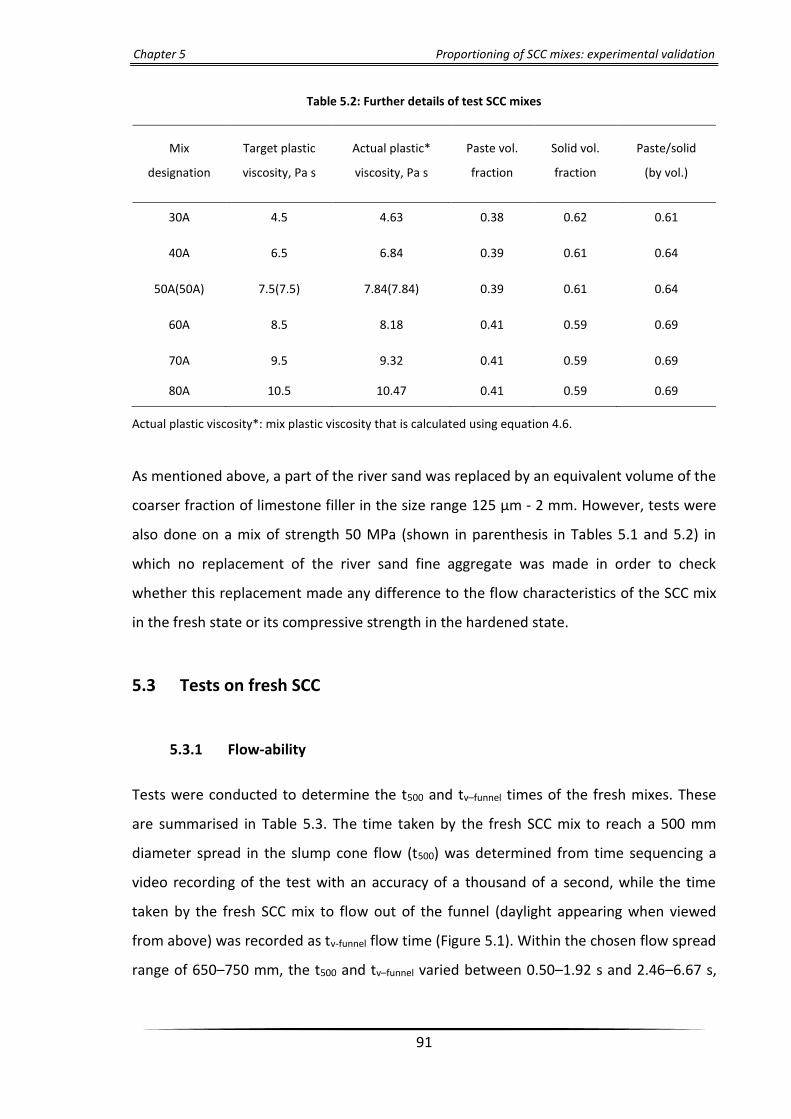
Chapter 5 Proportioning of SCC mixes: experimental validation
91
Table 5.2: Further details of test SCC mixes
Mix
designation
Target plastic
viscosity, Pa s
Actual plastic*
viscosity, Pa s
Paste vol.
fraction
Solid vol.
fraction
Paste/solid
(by vol.)
30A 4.5 4.63 0.38 0.62 0.61
40A 6.5 6.84 0.39 0.61 0.64
50A(50A) 7.5(7.5) 7.84(7.84) 0.39 0.61 0.64
60A 8.5 8.18 0.41 0.59 0.69
70A 9.5 9.32 0.41 0.59 0.69
80A 10.5 10.47 0.41 0.59 0.69
Actual plastic viscosity*: mix plastic viscosity that is calculated using equation 4.6.
As mentioned above, a part of the river sand was replaced by an equivalent volume of the
coarser fraction of limestone filler in the size range 125 μm - 2 mm. However, tests were
also done on a mix of strength 50 MPa (shown in parenthesis in Tables 5.1 and 5.2) in
which no replacement of the river sand fine aggregate was made in order to check
whether this replacement made any difference to the flow characteristics of the SCC mix
in the fresh state or its compressive strength in the hardened state.
5.3 Tests on fresh SCC
5.3.1 Flow-ability
Tests were conducted to determine the t500 and tv–funnel times of the fresh mixes. These
are summarised in Table 5.3. The time taken by the fresh SCC mix to reach a 500 mm
diameter spread in the slump cone flow (t500) was determined from time sequencing a
video recording of the test with an accuracy of a thousand of a second, while the time
taken by the fresh SCC mix to flow out of the funnel (daylight appearing when viewed
from above) was recorded as tv-funnel flow time (Figure 5.1). Within the chosen flow spread
range of 650–750 mm, the t500 and tv–funnel varied between 0.50–1.92 s and 2.46–6.67 s,

Chapter 5 Proportioning of SCC mixes: experimental validation
92
respectively. Figures 5.2-5.4 show the horizontal spread of different grade SCC mixes. All
test SCC mixes showed no signs of segregation or bleeding on thorough visual inspection.
Table 5.3: Flow-ability test results, t500 and tv–funnel of SCC mixes
Mix
designation
Slump flow test V–funnel test
Spread, mm t500, s tv–funnel, s
30A 685 0.50 2.46
40A 730 0.64 2.53
50A(50A) 675(670) 1.17(1.10) 3.37(3.28)
60A 665 1.18 3.23
70A 700 1.42 5.46
80A 730 1.92 6.67
Figure 5.1: Recording V-funnel time (daylight appearing when viewed from above)

Chapter 5 Proportioning of SCC mixes: experimental validation
93
Figure 5.2: Horizontal spread of SCC mix: 30A (Left), 50A (Right)
Figure 5.3: Horizontal spread of SCC mix: 60A (Left), 80A (Right)
Figure 5.4: Horizontal spread of SCC mix (50A)

Chapter 5 Proportioning of SCC mixes: experimental validation
94
A comparison of the flow tests on 50 MPa mix, in which a part of the river sand fine
aggregate was replaced by the coarser fraction of limestone filler with the same grade
mixes but without the replacement (shown in parenthesis in Table 5.3), shows that the
flow characteristics of the mixes are not significantly affected by this replacement. This is
consistent with the small differences in the particle size distributions of the coarser
fraction of limestone filler and river sand (Figure 5.5). Moreover, as the volume fractions
(not the masses) of the fine aggregate (with or without replacement) in the mixes are the
same (Tables 5.1 and 5.2), their plastic viscosity will be the same (see Eq. (4.6) in Chapter
4).
Figure 5.5: Particle size distribution curves for coarser fraction of limestone filler and fine aggregate
Figure 5.6 shows a plot of the flow time of all mixes and the corresponding water to
powder (i.e. cement + ggbs + limestone powder < 125 μm) ratio (w/p). It is seen that a
larger t500 requires a higher powder or lower water content. The w/p ratio has a
considerable influence on both the fresh and hardened properties of SCC, with often its
influence on the fresh properties limiting the selection of its value (Domone, 2006). It has
been reported that a decrease in the water content and an increase in the amount of fine
particles can increase cohesion and viscosity of the mix (Felekoǧlu et al., 2007), resulting
in a good distribution of the solid particles throughout the casting of SCC. However, mixes
0
20
40
60
80
100
0.01 0.1 1 10
Pas
sin
g, %
Sieve diameter, mm
Fine aggregate
Coarse LP

Chapter 5 Proportioning of SCC mixes: experimental validation
95
with low water content require relatively high dosages of super–plasticiser, especially at
low cm contents, to achieve the accepted requirements of SCC deformability (Khayat et
al., 1999).
Figure 5.6: Relationship between flow time (t500) and water to powder ratio
The time needed to reach 500 mm diameter spread is related to the plastic viscosity of
the mix. This is clearly seen in Figure 5.7 for a given target flow spread. Regarding the
plastic viscosity, it is worth mentioning that it is very difficult if not impossible to measure
it accurately. It is well known (Banfill et al., 2001; Feys et al., 2007; Wallevik and Wallevik,
2011) that for one and the same mix, different types of rheometer give different values of
Bingham parameters (plastic viscosity and yield stress). Therefore, the micromechanical
procedure proposed by Ghanbari and Karihaloo (2009) which calculates the plastic
viscosity of an SCC mix from the known plastic viscosity of the paste (which can be
accurately measured with a viscometer) has been recommended and used in this chapter.
This was already explained in Chapter 4 and indeed forms the basis of the proposed mix
proportioning method.
y = -0.9565x2 - 0.8205x + 3.0977R² = 0.9152
0.00
0.50
1.00
1.50
2.00
2.50
0.70 0.80 0.90 1.00 1.10 1.20 1.30
t 50
0, s
w/p, by volume

Chapter 5 Proportioning of SCC mixes: experimental validation
96
It should also be mentioned that the yield stress is well correlated with the slump flow
spread (Koehler and Fowler, 2007; Wallevick, 2003). That is why we have determined the
target flow spread of our mixes within the range of 700±50 mm. It is implied that these
mixes have nearly the same yield stress and thus make the plastic viscosity as the
controlling parameter which we have correlated with t500 in Figure 5.7. The following
statement from (Koehler and Fowler, 2007) supports this implicit assumption ‘‘the plastic
viscosity is often the main factor distinguishing the workability of one mix from another.
Changes in plastic viscosity can directly reflect changes in materials or mixture
proportions, making the t500 measurement particularly valuable for quality control’’. Of
course, a different choice of target plastic viscosity, say from the EFNARC (2005) will
necessarily require different t500.
The plastic viscosity has been plotted against tv–funnel and flow spread in Figure 5.8. It can
be seen that the tv–funnel of mixes having the flow spread in the range of 665–730 mm
increases with an increase in the mix plastic viscosity, despite an increase in the SP
dosage. In other words, the flow time is dominated by the plastic viscosity rather than
the SP dosage. This has also been observed by Nepomuceno et al. (2014) and Takada and
Tangtermsirikul (2000).
Figure 5.7: Relationship between plastic viscosity and t500 for target flow spread 700 ± 50 mm
y = 0.028x2 - 0.1766x + 0.6953R² = 0.9633
0
100
200
300
400
500
600
700
800
0.0
0.5
1.0
1.5
2.0
2.5
3.0
4.0 5.0 6.0 7.0 8.0 9.0 10.0 11.0
Spre
ad, m
m
t 50
0, s
Plastic viscosity, Pa.s
t500 Target spread Flow spread

Chapter 5 Proportioning of SCC mixes: experimental validation
97
Figure 5.8: Relationship between plastic viscosity and tv–funnel time with a target flow spread (700±50 mm)
5.3.2 Passing and filling ability
All the above test mixes that satisfied the flow-ability criterion and showed no signs of
segregation were subjected to the passing and filling ability test using the J–ring and L–
box (BS EN 206-9, 2010; EFNARC, 2005) to ensure that they were able to pass through the
narrow gaps that exist between reinforcing bars in real reinforced concrete structural
elements. For this purpose, two types of J-ring test have been used: wide gaps (10 bars)
and narrow gaps (16 bars) that are used for normal and congested reinforcement,
respectively. The results of the latter are presented in Table 5.4 whereas the former are in
Appendix C. There was a mix (60A which had a low flow spread, i.e. low dosage of SP) that
had passed the flow-ability test but did not meet the passing ability criterion. In this
instance, the SP dosage had to be increased (shown in square brackets in Table 5.1). The
results indicated that (after the increase in SP) all mixes met the passing ability criterion
and showed no blockage or signs of segregation (Figures 5.9 – 5.10). Again, the influence
of the replacement of some river sand fine aggregate by the coarser fraction of limestone
filler on the flow characteristics was minimal, as can be judged by comparing the entries
for 50 MPa mixes without and within the parenthesis in Table 5.4. Figure 5.11 shows that
t500j time correlates well with the plastic viscosity for all the mixes.
y = 0.1878x2 - 2.0755x + 8.0034R² = 0.9714
0
100
200
300
400
500
600
700
800
0.0
1.0
2.0
3.0
4.0
5.0
6.0
7.0
8.0
9.0
10.0
4.0 5.0 6.0 7.0 8.0 9.0 10.0 11.0
Spre
ad, m
m
t v-
fun
nel
, s
Plastic viscosity, Pa.s
t v- funnel Target spread Flow spread

Chapter 5 Proportioning of SCC mixes: experimental validation
98
Table 5.4: Passing ability test results, J–ring and L–box
Mix designation J–ring flow test L–box test
Spread, mm t500j, s t200, s t400, s H2/H1 or BR
30A 650 0.69 0.47 1.08 0.91
40A 700 0.80 0.50 0.91 0.92
50A(50A) 640 1.41 0.67(0.62) 1.40(1.35) 0.86(0.88)
60A 665 1.48 0.77 1.48 0.89
70A 690 2.04 1.25 2.66 0.88
80A 700 2.80 1.45 3.10 0.93
Figure 5.9: Flow and passing ability of SCC mix: 30A (Left), 40A (Right)
Figure 5.10: Flow and passing ability of SCC mix: 60A (Left), 70A (Right)

Chapter 5 Proportioning of SCC mixes: experimental validation
99
Figure 5.11: t500J time versus plastic viscosity
The relationship between the parameters t500 of J-ring and slump flow of SCC was also
taken into consideration in this study. The best-fit curve of t500 against the plastic viscosity
is plotted graphically alongside t500J in Figure 5.12. It was found that the difference
between these times is more pronounced in the higher plastic viscosities (8-10.5 Pa s)
than the lower ones. A possible explanation for this increase is that the mixes become
sticky taking more time to pass through the obstacles of the J-ring.
Figure 5.12: Plastic viscosity versus t500 and t500J
y = 0.0654x2 - 0.6213x + 2.1456R² = 0.9874
0.0
0.5
1.0
1.5
2.0
2.5
3.0
4.0 5.0 6.0 7.0 8.0 9.0 10.0 11.0
t 50
0J,
s
Plastic viscosity, Pa s
y = 0.028x2 - 0.1766x + 0.6953R² = 0.9633
y = 0.0654x2 - 0.6213x + 2.1456R² = 0.9874
0.0
0.5
1.0
1.5
2.0
2.5
3.0
4.0 5.0 6.0 7.0 8.0 9.0 10.0 11.0
Tim
e, s
Plastic viscosity, Pa s
t500 t500J-ring

Chapter 5 Proportioning of SCC mixes: experimental validation
100
According to the ASTM C 1621/ C 1621M (2008), the J-ring test can be used in
combination with the slump flow test to assess the passing ability of SCC. If the difference
between spread diameters (Dflow – DJ-ring) of the two tests is less than 25 mm then there is
no visible blockage. If it is between 25 and 50 mm then there is minimal to noticeable
blockage. Table 5.5 shows the difference from which it is clear that for all mixes there is
minimal or no blockage.
Table 5.5: Difference between flow and J-ring spread diameter
Mix designation Dflow, mm DJ-ring, mm Dflow – DJ-ring, mm
30A 685 650 35
40A 730 700 30
50A 675 640 35
60A 665 665 0
70A 700 690 10
80A 730 700 30
In order to test the ability of an SCC mix to fill the formwork containing reinforcement
under its own weight, the L–box apparatus with two adjustable steel rods (each of
diameter 12 mm) was used (12350-10, 2010; EFNARC, 2005). The times for the mix to
reach 200 mm (t200) and 400 mm (t400) from the vertical leg as well as the blockage ratio
(BR or H2/H1) were recorded. All mixes that had passed the J–ring test also passed the L–
box test without any alteration in SP or mix ingredients (Figures 5.13–5.15). Figure 5.16
shows that t200 and t400 times correlate well with the plastic viscosity for all the mixes. The
results also showed that no large aggregate particles had segregated or been blocked by
the rods. Also, it can be seen (Table 5.4) that the mixes exhibited a blockage ratio (BR) of
more than 0.80, which reflects good filling ability.

Chapter 5 Proportioning of SCC mixes: experimental validation
101
Therefore, from the flow and passing ability perspectives, all the test SCC mixes satisfied
the required criteria for viscosity class 1 to qualify them as SCC in accordance with BS–EN
206–9 (2010).
Figure 5.13: Passing and filling of SCC mix: 30A (Left), 40A (Right)
Figure 5.14: Passing and filling of SCC mix: 60A (Left), 80A (Right)

Chapter 5 Proportioning of SCC mixes: experimental validation
102
Figure 5.15: Passing and filling of SCC mix (50A)
Figure 5.16: t200 and t400 times in L-box versus plastic viscosity
In Figures 5.7, 5.8, 5.11, 5.12 and 5.16, a bi-linear regression approximation was also
explored. However, it was found in each case that the R2 value is less than that shown in
the respective figures.
y = 0.0385x2 - 0.3984x + 1.4716R² = 0.9622
y = 0.1008x2 - 1.1356x + 4.115R² = 0.9478
0.0
0.5
1.0
1.5
2.0
2.5
3.0
3.5
4.0 5.0 6.0 7.0 8.0 9.0 10.0 11.0
Tim
e, s
Plastic viscosity, Pa s
t200 t400

Chapter 5 Proportioning of SCC mixes: experimental validation
103
5.4 Testing of hardened SCC
The accuracy of the proposed design method has been validated through compressive
strength tests performed on 100 mm cube specimens (three per mix and age), cured in
water at ambient temperature. The results are presented in Table 5.6 and Figure 5.17.
The test was carried out at 7, 28 and 90 days of age. The results confirm the well–known
trends against the w/cm ratio and confirmed the reliability of the proposed mix–design
approach. The effect of the replacement of a part of the river sand fine aggregate by the
coarser fraction of limestone powder is minimal also in the hardened state, as can be
judged by the entries in the parenthesis in Table 5.6.
Table 5.6: Cube compressive strength test results for SCC mixes
Mix designation
Compressive strength, MPa
7 days 28 days 90 days
30A 24.3 37.2 45.7
40A 30.9 44.5 51.2
50A(50A) 35.6 50.9(50.1) 55.1
60A 43.2 62.7 72.6
70A 48.0 74.8 89.4
80A 56.5 80.9 91.4

Chapter 5 Proportioning of SCC mixes: experimental validation
104
Figure 5.17: Gain of compressive strength with age
5.5 Concluding remarks
This chapter was concerned with the experimental validation of the mix design method
proposed in Chapter 4. Several mixes proportioned with the method proposed in the
previous chapter were prepared in the laboratory and found to meet the necessary self-
compacting criteria and the target plastic viscosity and compressive strength, thus fully
validating the proposed mix proportioning method.
It may however be necessary to increase the SP content in order to meet the passing and
filling ability tests, but the content will still be in the range 0.4-0.6% of the mass of
cementitious materials. It is worth emphasising that the plastic viscosity of the paste
remains practically unaltered in this range; the SP content mostly affects the yield stress
of the paste.
The coarser fraction of limestone filler (125 μm – 2 mm) can be used to replace an
equivalent volume of river sand fine aggregate. Tests have shown that this replacement
makes practically no difference to the properties of SCC in fresh and hardened tests. Such
20
30
40
50
60
70
80
90
100
0 20 40 60 80 100
Cu
be
com
pre
ssiv
e st
ren
gth
, MP
a
Age, days
30 MPa 40 MPa 50 MPa
60 MPa 70 MPa 80 MPa

Chapter 5 Proportioning of SCC mixes: experimental validation
105
a replacement is environmentally friendly and economic, thus enhancing the
sustainability of the SCC mixes.
The proposed mix proportioning method is simple and leads to mix proportions that
indeed are self-compacting concrete. It reduces considerably the extent of laboratory
work, the testing time and the materials used.

Influence of mix composition and strength on
the fracture properties of SCC

Chapter 6 Influence of mix composition and strength on the fracture properties of SCC
107
6.1 Introduction
Self-compacting concrete (SCC) has undergone extensive investigations that have led to
confidence in its fresh and hardened properties, yet its composition variations raise
concerns as to its fracture behaviour. This chapter presents the results of an experimental
study on fracture behaviour of SCC mixes differing by the coarse aggregate volume (CA),
paste to solids ratio (p/s) and water to binder (or cementitious material (w/cm)) ratio.
First the size-dependent fracture energy (𝐺𝑓) has been determined using the RILEM work-
of-fracture test on three point bend specimens of a single size, half of which contained a
shallow starter notch (notch to depth ratio = 0.1), while the other half contained a deep
notch (notch to depth ratio = 0.6). Then the specific size-independent fracture energy
(𝐺𝐹) was calculated using the simplified boundary effect formalism in which the variation
in the fracture energy along the unbroken specimen ligament is approximated by a
bilinear diagram. Finally, the bilinear approximation of the tension softening diagram
(TSD) corresponding to 𝐺𝐹 has been obtained using the non-linear hinge model.
The contents of this chapter have been published in the journal ‘Construction and
Building Materials’ (see publication 6 in the list in Chapter 1).
6.2 Fracture behaviour of SCC
The fracture behaviour of concrete is significantly influenced by the properties of the
interfacial transition zone (ITZ) (Akçaoǧlu et al., 2004), which in turn are governed by the
mix ingredients in vibrated concrete (VC) and self-compacting concrete (SCC), as well. In
comparison with VC, SCC requires relatively high amounts of fine particles and paste, but
low coarse aggregate content (Okamura and Ouchi, 2003; Okamura et al., 2000;
Edamatsu et al., 1998; Su et al., 2001). Although SCC has passed from the research phase
into real application, the differences in its composition from VC raise concerns about its
fracture behaviour (Beygi et al., 2014a,b,c; Domone, 2006). The concern is primarily
because a lower coarse aggregate content in an SCC mix relative to a VC mix of the same
grade is likely to reduce its energy absorption capacity and thus its ductility. This needs to
be addressed. Previous work (Beygi et al., 2014a,b,c; Nikbin et al., 2014b,c; Cifuentes and

Chapter 6 Influence of mix composition and strength on the fracture properties of SCC
108
Karihaloo, 2013; Beygi et al., 2013a; Rozière et al., 2007) on this topic was based on the
size-dependent specific fracture energy, apart from the work of Cifuentes and Karihaloo
(2013) who used the model of Hu and Wittmann (2000) and its simplified version
proposed by Karihaloo et al. (2003).
It is the aim of the present chapter to investigate in detail the role of several composition
parameters of SCC mixes in their fracture behaviour. In particular, the influence of coarse
aggregate volume (CA), paste to solids (p/s) and water to binder (w/cm) ratios on the
size-independent fracture energy (𝐺𝐹) will be studied using the simplified boundary effect
approach (SBE) suggested by Abdalla and Karihaloo (2003) and validated by Karihaloo et
al. (2003). The corresponding bilinear approximation of the tension softening diagram will
then be obtained using the procedure based on the non-linear hinge model proposed by
Abdalla and Karihaloo (2004), and Murthy et al. (2013a).
6.3 Parameters describing the fracture behaviour of concrete
Specific fracture energy and the tension softening diagram of a concrete mix are the most
important parameters describing its fracture behaviour. They form a basis for the
evaluation of the load carrying capacity of cracked concrete structures (Karihaloo, 1995;
Bazant and Planas, 1997). These parameters are explained below.
6.3.1 Specific fracture energy
According to RILEM recommendations (RILEM-50FMC, 1985), the specific fracture energy
(or toughness) can be obtained by the work-of-fracture method requiring tests on
notched three-point bend specimens of different sizes and notch to depth ratios.
It is however widely recognised (Abdalla and Karihaloo, 2003; Bažant, 1996; Bažant and
Kazemi, 1991; Carpinteri and Chiaia, 1996; Hu and Wittmann, 1992; Mindess, 1984;
Nallathambi et al., 1985) that the specific fracture energy of concrete obtained using the
RILEM method is dependent on the size of the test specimen and the notch to depth
ratio. To eliminate this size dependency, Guinea and co-workers (Guinea et al., 1992;
Planas et al., 1992; Guinea et al., 1994) and Hu and Wittmann (2000) proposed methods

Chapter 6 Influence of mix composition and strength on the fracture properties of SCC
109
to correct the measured size-dependent specific fracture energy (𝐺𝑓) in order to obtain a
size-independent value (𝐺𝐹). The methodology proposed by Guinea and co-workers
(Guinea et al., 1992; Planas et al., 1992; Guinea et al., 1994) involves adding the non-
measured work-of-fracture due to the curtailment of the tail of the load-central
deflection (Ρ-δ) curve recorded in the three-point bend test. On the other hand, the
methodology of Hu and Wittmann (2000) is based on the observation that the local
specific energy along the initially un-cracked specimen ligament varies during the crack
propagation, the variation becomes more pronounced as the crack approaches the stress-
free back face of the specimen, the so-called free boundary effect.
Abdalla and Karihaloo (2003) and Karihaloo et al. (2003) simplified the free boundary
effect formalism of Hu and Wittmann (2000). They proposed and validated extensively a
simplified method by which the size-independent fracture energy can be determined by
testing only geometrically identical specimens of the same size, half of which contain a
shallow starter notch (notch to depth ratio = 0.1), while the other half contain a deep
notch (notch to depth ratio = 0.6). Their method significantly reduces the number of
specimens to be tested and eliminates the need for using the least squares method to
solve an over-determined system of simultaneous equations, as required in the Hu and
Wittmann (2000) method.
6.3.2 Tension softening diagram (TSD)
Besides the size-independent fracture energy (𝐺𝐹), the analysis of cracked concrete
structures using the non-linear fictitious crack model (Hillerborg et al., 1976) requires the
tension softening diagram, σ(w) of the concrete mix relating the residual stress transfer
capability (σ) to the opening displacement (w) of the fictitious crack faces. As the
determination of the tension softening diagram using the direct tension test is not a
simple task (Karihaloo, 1995), it is often approximated by a bilinear relationship whose
parameters are determined in an inverse manner by matching the experimental load-
displacement curve of a notched three-point bend beam. For this an analytical model
based on the concept of a non-linear hinge was proposed by Ulfkjær et al. (1995) and

Chapter 6 Influence of mix composition and strength on the fracture properties of SCC
110
Olesen (2001). In this model, the flexural response of a notched beam is obtained by
allowing the fictitious crack to develop from the pre-existing notch in the central region of
the beam where the bending moment is the largest. The width of this region,
proportional to the beam depth, fixes the width of the non-linear hinge. Outside of this
region, the material is assumed to behave in a linear elastic manner. Abdalla and
Karihaloo (2004) and Murthy et al. (2013a) showed how the non-linear hinge model can
be adapted to construct the bilinear tension softening diagram of a concrete mix
corresponding to its size-independent specific fracture energy (𝐺𝐹).
6.4 Theoretical background
The specific fracture energy (𝐺𝑓), as defined by RILEM technical committee TC50, is the
average energy given by dividing the total work of fracture by the projected fracture area
(i.e. cross-section of initially un-cracked ligament) based on the load-displacement P-δ
curve. Hence, for a specimen of depth W, thickness B and initial notch depth a (as
schematically shown in Figure 6.1), the specific fracture energy (𝐺𝑓) can be expressed as:
𝐺𝑓 =1
(𝑤−𝑎)𝐵∫𝑃𝑑𝛿 (6.1)
The specimen weight can be neglected for the small specimens used in this study.

Chapter 6 Influence of mix composition and strength on the fracture properties of SCC
111
(Shallow notch) (Deep notch)
Figure 6.1: Schematic representation of the three-point bending test
The specific fracture energy (𝐺𝑓) can also be determined using a local energy (gf) concept
described by Duan et al. (2003; 2007) as follows (see Figure 6.2):
𝐺𝑓 (𝑎
𝑊) =
1
𝑤−𝑎∫ 𝑔𝑓(𝑥)𝑑𝑥𝑤−𝑎
0 (6.2)
Hu and Wittman (2000) proposed a bilinear approximation for the local fracture energy
variation (𝑔𝑓) along the crack path (Figure 6.2) with the intersection of the two
asymptotes defining a transition ligament size (𝑎𝑙). The latter, unlike the asymptotic value
of specific fracture energy (𝐺𝐹), varies with the material properties and specimen
geometry.

Chapter 6 Influence of mix composition and strength on the fracture properties of SCC
112
Figure 6.2: Bilinear local fracture energy 𝑮𝒇 (𝒂
𝑾) variation along the un-notched ligament of a notched
specimen (After: Duan et al., 2003)
A relation between the measured size-dependent fracture energy (𝐺𝑓), the transition
length (𝑎𝑙) and the size-independent fracture energy (𝐺𝐹) can be obtained by substituting
the bilinear approximation for the local fracture energy variation (Figure 6.2) into Eq. (6.2)
𝐺𝑓 (𝑎
𝑊) =
{
𝐺𝐹 [1 −
𝑎𝑙𝑊
2(1−𝑎
𝑊)] 1 −
𝑎
𝑊 >
𝑎𝑙
𝑊
𝐺𝐹 [(1−
𝑎
𝑊)
2 𝑎𝑙𝑊
] 1 −𝑎
𝑊 ≤
𝑎𝑙
𝑊
(6.3)
The values of 𝐺𝐹 and 𝑎𝑙 of a concrete mix are obtained once the mean size-dependent
specific fracture energy (𝐺𝑓) of the mix has been measured on specimens of identical
sizes, half of which have a shallow starter notch (a/W = 0.1), while the other half have a
deep starter notch (a/W = 0.6) by the RILEM work-of-fracture method using Eq. (6.1). Hu
and Duan (2004) showed that although the measured values of 𝐺𝑓 depend on W and a/W,
the above procedure indeed leads to a 𝐺𝐹 value that is essentially independent of the
specimen size and relative notch depth.
In recent works, a trilinear approximation of the local fracture energy along the unbroken
ligament was proposed by Muralidhara et al. (2010; 2011) and Karihaloo et al. (2013). As
has been evidenced by acoustic emission data, the trilinear approximation is closer to
how the local fracture energy varies as the crack grows from a notched specimen
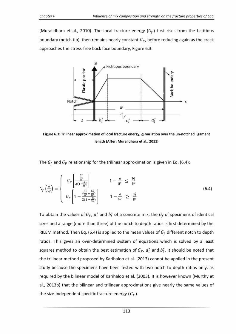
Chapter 6 Influence of mix composition and strength on the fracture properties of SCC
113
(Muralidhara et al., 2010). The local fracture energy (𝐺𝑓) first rises from the fictitious
boundary (notch tip), then remains nearly constant 𝐺𝐹, before reducing again as the crack
approaches the stress-free back face boundary, Figure 6.3.
Figure 6.3: Trilinear approximation of local fracture energy, gf variation over the un-notched ligament
length (After: Muralidhara et al., 2011)
The 𝐺𝑓 and 𝐺𝐹 relationship for the trilinear approximation is given in Eq. (6.4):
𝐺𝑓 (𝑎
𝑊) =
{
𝐺𝐹 [
𝑏𝑙∗
𝑊
2(1−𝑎
𝑊)] 1 −
𝑎
𝑊 ≤
𝑏𝑙∗
𝑊
𝐺𝐹 [1 −(𝑎𝑙∗
𝑊 +
𝑏𝑙∗
𝑊)
2(1 − 𝑎
𝑊) ] 1 −
𝑎
𝑊 ≥
𝑎𝑙∗
𝑊
(6.4)
To obtain the values of 𝐺𝐹, 𝑎𝑙∗ and 𝑏𝑙
∗ of a concrete mix, the 𝐺𝑓 of specimens of identical
sizes and a range (more than three) of the notch to depth ratios is first determined by the
RILEM method. Then Eq. (6.4) is applied to the mean values of 𝐺𝑓 different notch to depth
ratios. This gives an over-determined system of equations which is solved by a least
squares method to obtain the best estimation of 𝐺𝐹, 𝑎𝑙∗ and 𝑏𝑙
∗. It should be noted that
the trilinear method proposed by Karihaloo et al. (2013) cannot be applied in the present
study because the specimens have been tested with two notch to depth ratios only, as
required by the bilinear model of Karihaloo et al. (2003). It is however known (Murthy et
al., 2013b) that the bilinear and trilinear approximations give nearly the same values of
the size-independent specific fracture energy (𝐺𝐹).

Chapter 6 Influence of mix composition and strength on the fracture properties of SCC
114
6.5 Experimental programme
6.5.1 Materials
Locally available type ІІ cement (CEM II/B-V 32.5R according to BS EN 197-1 (2011)) and
ground granulated blast furnace slag (ggbs) with a specific gravity of 2.95 and 2.40,
respectively were used. The super-plasticiser used was a poly-carboxylic ether-based type
with specific gravity of 1.07. Crushed limestone coarse aggregate with a maximum size of
20 mm and a specific gravity of 2.80 was used, while the fine aggregate was river sand
having a specific gravity of 2.65. Limestone powder as filler with maximum particle size of
125 μm was used (specific gravity 2.40). A part of the river sand was replaced by an
equivalent volume of the coarser fraction of limestone filler in the size range 125 μm - 2
mm.
6.5.2 Mix design
A series of SCC mixes were designed according to the procedure described in Chapter 4
having 28-day nominal cube compressive strengths of 30, 60 and 80 MPa with w/cm
ratios of 0.63, 0.47 and 0.35, respectively. The SCC mixes contained low paste to solid
(p/s) ratio. They are designated A. They have been combined with mixes of medium p/s,
designated B, that were studied by Alyhya (2016) and with mixes of high p/s, designated
C, that were studied by Al-Rubaye (2016), in order to get a complete picture of the role of
low, medium and high p/s ratios (as will be explained later). The compositions of all mixes
are given in Table 6.1. In order to ensure that all mixes met the flow and passing ability
criteria without segregation (SCC requirements), slump flow, J-ring, L-box and V-funnel
tests were conducted (Table 6.2) according to BS EN 206-9 (2010) and EFNARC (2005).

Chapter 6 Influence of mix composition and strength on the fracture properties of SCC
115
Table 6.1: Mix proportions of test SCC mixes, kg/m3
Mix
desig.
cm a
w
SP b
w/c
m
SP/cm
%
LP c
FA d
CA e
p/s
by
vol. cement ggbs FA** FA ***
30A* 240 80 201.6 1.4 0.63 0.44 109 164 579 924 0.61
30B* 240 80 201.6 1.6 0.63 0.50 156 234 530 840 0.67
30C* 240 80 201.6 2.3 0.63 0.72 194 291 504 756 0.72
60A 315 105 197.5 2.3 0.47 0.55 94 141 536 924 0.69
60B 315 105 197.5 2.4 0.47 0.57 125 188 528 840 0.72
60C 315 105 197.5 2.8 0.47 0.67 172 258 477 756 0.79
80A 367.5 122.5 171.5 2.8 0.35 0.57 94 141 536 924 0.69
80B 367.5 122.5 171.5 3.0 0.35 0.61 125 188 529 840 0.72
80C 367.5 122.5 171.5 3.5 0.35 0.71 172 258 478 756 0.79
*A, B and C indicate decrease in coarse aggregate and increase in paste volume for the same strength grade.
a: cementitious material, i.e. binder.
b: super-plasticiser.
c: limestone powder<125 μm.
d: fine aggregate<2 mm (Note: a part of the fine aggregate is the coarser fraction of the limestone
powder, FA**125 μm -2 mm, whereas FA *** refers to natural river sand<2 mm).
e: coarse aggregate <20 mm.

Chapter 6 Influence of mix composition and strength on the fracture properties of SCC
116
Table 6.2: Flow and passing ability test results of SCC mixes
Mix designation
Slump flow V-funnel J–ring flow test L–box test
Spread
mm
t500
s
tv–funnel
s
Spread
mm
t500J
s
t200
s
t400
s H2 / H1
30A 685 0.50 2.46 650 0.70 0.47 1.08 0.91
30B 665 0.88 2.47 635 1.04 0.57 1.11 0.84
30C 655 0.81 2.76 650 0.74 0.53 1.10 0.92
60A 665 1.18 3.23 665 1.48 0.77 1.48 0.89
60B 650 1.32 3.54 645 1.43 0.81 1.72 0.84
60C 655 1.40 4.04 630 1.60 0.81 1.65 0.87
80A 730 1.92 6.67 700 2.80 1.45 3.10 0.93
80B 750 2.06 7.34 730 2.70 1.62 3.20 0.90
80C 670 2.09 7.44 655 2.80 1.45 3.07 0.91
6.6 Specimen preparation and test procedure
From each of the nine mixes (Table 6.1) 12 beam specimens (Figure 6.1), three cubes (100
mm), and three cylinders (100 x 200 mm) were cast. The specimens were de-moulded
after one day and cured in water at ambient temperature for 28 days. The cube
compressive strength was measured according to BS EN 12390-3 (2009). Six of the beams
were notched to a depth of 10 mm (notch to depth ratio a/W = 0.1) (Figure 6.4a), with a
thin (2 mm) diamond saw while the remaining six were notched to a depth of 60 mm
(a/W = 0.6) (Figure 6.4b). The split cylinder strength (fst) and the modulus of elasticity (E)
were measured on cylinders according to BS EN 12390-6 (2009) and BS 1881-121 (1983),
respectively.

Chapter 6 Influence of mix composition and strength on the fracture properties of SCC
117
(a) (b)
Figure 6.4: (a) shallow notch to depth ratio (0.1), (b) deep notch to depth ratio (0.6)
As schematically shown in Figure 6.1, the tests for the determination of the fracture
energy were performed according to the RILEM work-of-fracture method (RILEM-50FMC,
1985). The crack mouth opening displacement (CMOD) was used as the feedback control
signal and the load-point deflection was measured simultaneously by means of a linearly
variable displacement transducer (LVDT). The tests were performed in a stiff Dartec
closed-loop universal testing machine with a maximum load capacity of 250 kN.
6.7 Results and discussion
Typical recorded load-deflection diagrams of three of the nine mixes are shown in Figure
6.5. The individual specimen curves for load-deflection and load-CMOD are given in
Appendix D and Appendix E, respectively. The area under the load-deflection diagram was
calculated from which the 𝐺𝑓(a,W) was determined using Eq. (6.1). Table 6.3 shows the
results of the measured fracture energy 𝐺𝑓(a,W), with an indication of the mean value,
standard deviation and the coefficient of variation (COV%).

Chapter 6 Influence of mix composition and strength on the fracture properties of SCC
118
Table 6.3: Measured fracture energy, 𝑮𝒇(a,W) for different SCC mixes from three point bending test (TPB)
Mix designation
W, mm
a/W Mean [St. dev.]
𝑮𝒇(a,W), N/m COV, %
30A 100
0.1 96.20 [8.90] 9.20
0.6 53.50 [5.00] 9.30
30B 100
0.1 85.90 [7.70] 9.00
0.6 53.00 [4.00] 7.60
30C 100
0.1 73.40 [7.30] 10.0
0.6 52.30 [4.30] 8.20
60A 100
0.1 108.6 [11.6] 10.7
0.6 65.80 [1.70] 2.60
60B 100
0.1 91.90 [5.70] 6.20
0.6 56.50 [5.00] 8.85
60C 100
0.1 83.90 [9.60] 11.4
0.6 51.90 [3.20] 6.10
80A 100
0.1 105.5 [5.50] 5.30
0.6 58.50 [5.70] 9.80
80B 100
0.1 100.1 [9.90] 9.90
0.6 57.00 [4.90] 8.60
80C 100
0.1 97.60 [11.0] 11.3
0.6 57.70 [2.50] 4.30

Chapter 6 Influence of mix composition and strength on the fracture properties of SCC
119
Figure 6.5: Typical load–displacement diagrams of two notched beams (out of twelve tested) from SCC
mixes: 30A (top), 60A (middle), and 80A (bottom)

Chapter 6 Influence of mix composition and strength on the fracture properties of SCC
120
The specific size-independent fracture energy (𝐺𝐹) and the transition ligament lengths
(𝑎𝑙) of all mixes are determined from 𝐺𝑓(0.1) and 𝐺𝑓(0.6) of Table 6.3 using the first of the
two equalities in Eq. (6.3). In many mixes, however it transpired that the transition
ligament length (𝑎𝑙) so calculated violated the corresponding inequality for a/W = 0.6. In
these cases the first of the two equalities was used only for a/W = 0.1, while the second
equality was used for the deeper notch a/W = 0.6. The resulting values of 𝐺𝐹 and 𝑎𝑙 are
reported in Table 6.4, together with the cube compressive strength (𝑓𝑐𝑢), split cylinder
strength (𝑓𝑠𝑡) and modulus of elasticity (E), measured according to the relevant British
standards.
Table 6.4: Results of 𝒇𝒄𝒖, 𝒇𝒔𝒕, E, 𝑮𝑭 and 𝒂𝒍 of test SCC mixes
Mix designation 𝑓𝑐𝑢, 28 days
MPa 𝑓𝑠𝑡, 28 days
MPa 𝐸, 28 days GPa
𝐺𝐹
N/m
𝑎𝑙
mm
30A 35.4 2.95 33.6 132.8 49.7
30B 37.0 3.04 32.7 112.3 42.4
30C 37.8 3.30 32.0 90.4 33.8
60A 60.5 3.40 36.7 143.2 43.6
60B 62.9 3.52 36.6 120.3 42.6
60C 65.2 3.65 34.5 109.7 42.3
80A 79.8 4.60 42.3 146.9 50.7
80B 81.6 5.00 40.8 136.5 47.9
80C 83.2 5.35 41.0 130.2 45.2
Within the range of coarse aggregate volume fraction (27-33%) investigated in this study,
𝐺𝐹 increases with the increase of coarse aggregate fraction as is clear from Table 6.4 and
Figure 6.6 because of the increase in the energy dissipation mechanisms (micro-cracking,
crack branching, aggregate interlock) in much the same manner as in VC (Karihaloo, 1995;
Akcay et al., 2012; Prokopski and Langier, 2000). This observation is in agreement with
previous research on SCC (Beygi et al., 2014c; Nikbin et al., 2014b).

Chapter 6 Influence of mix composition and strength on the fracture properties of SCC
121
Moreover, it can be seen from Figure 6.6 that the increase in 𝐺𝐹 with the coarse
aggregate volume fraction is less pronounced in the high strength mix (grade 80) than in
mix grades 30 and 60. This is may be attributed to the fact that the ITZ (Beygi et al.,
2014b) in grade 80 mixes is much denser and therefore more susceptible to cracking
because it contains a higher proportion of cementitious materials, as can be seen in Table
6.1.
Figure 6.6: Variation of 𝑮𝑭 of SCC mixes of different grades with coarse aggregate volume fraction
An increase in the paste to solids (p/s) ratio in all mix grades, as expected, leads to a slight
increase in the cube compressive strength (fcu) but a noticeable decrease in 𝐺𝐹 , as shown
in Figure 6.7.
80
100
120
140
160
26 27 28 29 30 31 32 33 34
GF
, N/m
Coarse aggregate volume fraction, %
Grade 80
Grade 60
Grade 30

Chapter 6 Influence of mix composition and strength on the fracture properties of SCC
122
Figure 6.7: Variation of the 𝑮𝑭 and 𝒇𝒄𝒖 with different p/s ratios.
As expected, 𝐺𝐹 decreases with increasing water to binder (w/cm) ratio, in much the
same manner as in VC (Prokopski and Langier, 2000; Nallathambi et al., 1984) as shown in
Figure 6.8. This result is consistent with the recent study on normal strength self-
compacting concrete conducted by Beygi et al. (2013a) who found that fracture energy
decreases by 38% as w/cm ratio is increased from 0.4 to 0.7. 𝐺𝐹 of high strength self-
compacting concrete (fcu ~ 100 MPa), on the other hand has been reported by Cifuentes
and Karihaloo (2013) to be just 90 N/m for w/cm = 0.23. This is a consequence of the
densification of ITZ as a result of using a fairly high volume fraction of micro-silica.
Figure 6.8: Variation in 𝑮𝑭 with w/cm ratio for different coarse aggregate (CA) volume fractions
60
80
100
120
140
160
0.3 0.4 0.5 0.6 0.7
GF,
N/m
w/cm
33% CA (The present study)
30% CA (Alyhya, 2016)
27% CA (Al-Rubaye, 2016)

Chapter 6 Influence of mix composition and strength on the fracture properties of SCC
123
6.8 Bilinear tension softening diagram
To complete the determination of the fracture properties of the SCC mixes, we now
outline briefly an inverse procedure based on the non-linear hinge concept for identifying
the parameters of the bilinear tension softening diagrams of the mixes corresponding to
their above size-independent values of the specific fracture energy (𝐺𝐹). The details of
the procedure may be found in (Abdalla and Karihaloo, 2004; Murthy et al., 2013a). It
should be mentioned that the popularity of the bilinear approximation of the tension
softening diagram (Figure 6.9) stems from the fact that it captures the two major
mechanisms responsible for the observed tension softening in a concrete mix, namely
micro-cracking and frictional aggregate interlock. The initial linear branch of the bilinear
diagram which is steep is a consequence of the micro-cracking, whereas the second linear
branch which is shallow is a result of the frictional aggregate interlock.
Figure 6.9: Bilinear softening diagram
In the non-linear hinge model of a pre-notched beam, a part of the beam on either side of
the notch is isolated as a short beam segment subjected to a bending moment and a
normal force. The growth of the real crack and associated fictitious crack representing the
fracture process zone is viewed as a local change in the overall stress and strain fields in
this isolated beam segment.

Chapter 6 Influence of mix composition and strength on the fracture properties of SCC
124
The constitutive relationship inside the hinge segment depends on the position of the
fictitious crack along the depth of the beam. The axial load and bending moment are
related to the hinge rotation in four phases depending on the crack propagation. Phase 0
represents the elastic state when no fictitious crack has formed ahead of the pre-existing
notch. Phases I, II and III represent different stages of crack propagation. In phase I, the
fictitious crack ahead of the notch is such that the maximum crack opening is less than 𝑤1
corresponding to the knee in the bilinear diagram. In phase II, a part of the fictitious crack
of length longer than d has a width in excess of 𝑤1, but in the remaining part it is less than
𝑤1. In phase III, a part of the fictitious crack has opened more than 𝑤𝑐 and thus become
traction-free, while the opening of the remaining part is still less than 𝑤𝑐 or even 𝑤1.
Analytical expressions relating the hinge rotation to the bending moment and crack
length in each phase, and in turn to the applied central load on the beam and crack
mouth opening displacement (CMOD) are given in Abdalla and Karihaloo (2004). The
expressions for CMOD and central load are used to minimise the sum of squares of the
error between the theoretical and experimental values of the load with respect to the
three unknown parameters of the bilinear tension softening diagram (Figure 6.9). The
accuracy of this minimization procedure depends on the total number of observations
from the recorded load-CMOD diagram used in this procedure and the allowable error
(<3%). For this purpose, a MATLAB program was written and is given in Appendix F. The
load-CMOD curves generated by the hinge model and average experimental load-CMOD
curves are shown in Figure 6.10.
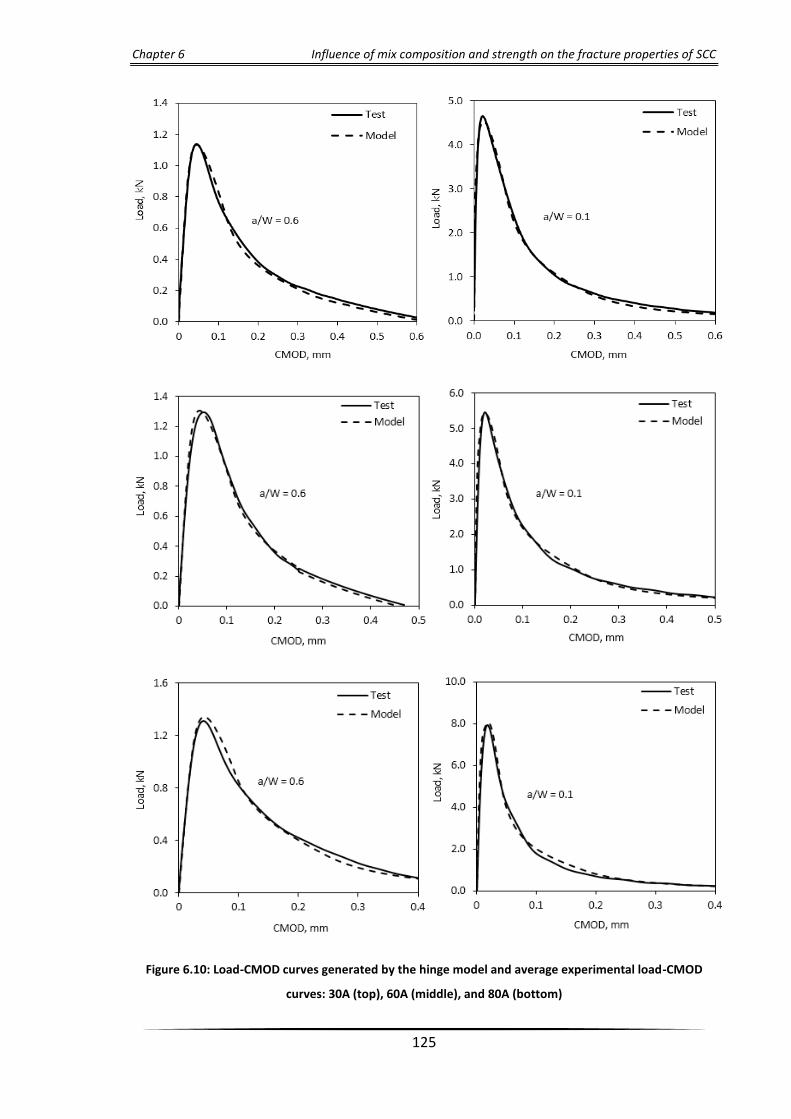
Chapter 6 Influence of mix composition and strength on the fracture properties of SCC
125
Figure 6.10: Load-CMOD curves generated by the hinge model and average experimental load-CMOD
curves: 30A (top), 60A (middle), and 80A (bottom)

Chapter 6 Influence of mix composition and strength on the fracture properties of SCC
126
As the load-CMOD diagrams are recorded on tests on beams with a notch to depth ratio
of 0.1 or 0.6, the three unknown parameters of the bilinear tension softening diagram
obtained from the above minimization procedure correspond not to the 𝐺𝐹 of the SCC
mix but to its size-dependent 𝐺𝑓(0.1) and 𝐺𝑓(0.6). These pairs of three parameters need
therefore to be appropriately scaled to reflect the size-independent 𝐺𝐹 of the mix. The
scaling procedure is described in Abdalla and Karihaloo (2004).
The bilinear tension softening diagrams of all nine SCC mixes corresponding to their 𝐺𝐹
are shown in Figure 6.11. The three parameters describing the shape of the bilinear
diagram, together with the direct tensile strength (fct) and the elastic modulus (E) of all
SCC mixes are given in Table 6.5. The slope of the initial part of the bilinear softening
curve increases with the increasing the p/s ratio, but the influence of p/s decreases as the
𝑓𝑐𝑢 of the mix increases. In addition, the critical crack opening (𝑤𝑐) is dominated by the
coarse aggregate volume in the mix and the mix grade. The larger the coarse aggregate
volume the larger is the critical crack opening (𝑤𝑐). However, the higher the mix grade the
lower is the critical crack opening (𝑤𝑐) (Figure 6.11).
Table 6.5: Parameters of the bilinear softening diagram corresponding to 𝑮𝑭
Mix
Designation
a1
mm-1
a2
mm-1
w1
mm
wc
mm
𝜎
𝑓𝑡
𝐺𝐹
N/m
E
GPa
𝑙𝑐ℎ
mm
30A 10.07 1.12 0.078 0.272 0.218 132.8 33.6 1377
30B 13.21 1.05 0.060 0.254 0.203 112.3 32.7 976
30C 18.76 1.20 0.043 0.198 0.186 90.4 32.0 519
60A 10.97 1.14 0.073 0.251 0.203 143.2 36.7 1057
60B 13.17 1.25 0.062 0.213 0.189 120.3 36.6 771
60C 15.38 1.28 0.053 0.198 0.185 109.7 34.5 497
80A 16.19 1.18 0.048 0.238 0.225 146.9 42.3 647
80B 18.51 1.39 0.043 0.194 0.211 136.5 40.8 380
80C 19.75 1.38 0.041 0.177 0.188 130.2 41.0 289

Chapter 6 Influence of mix composition and strength on the fracture properties of SCC
127
Figure 6.11: The normalised bilinear stress-crack opening relationship for SCC mixes corresponding to
their 𝑮𝑭

Chapter 6 Influence of mix composition and strength on the fracture properties of SCC
128
6.9 Direct and indirect tensile strengths and characteristic length of test
SCC mixes
It is well documented that the direct tensile strength (𝑓𝑐𝑡) is approximately two thirds of
the indirect tensile strength (𝑓𝑠𝑡) for VC (Neville, 1996). Although the literature is rich in
reporting on SCC, the effect of p/s ratio and mix grade on tensile strength is still not fully
addressed. The relationship between the direct tensile strength (determined by the
inverse analysis using the non-linear hinge model) and splitting strengths (𝑓𝑐𝑡/𝑓𝑠𝑡) of SCC
mixes of different p/s ratio and mix grade are summarised in Table 6.6 and Figure 6.12. It
is found that 𝑓𝑐𝑡/𝑓𝑠𝑡 is dominated by the p/s in the mix and the mix grade: it increases
with both an increase in p/s and mix grade. This might provide a better understanding of
the effect of p/s on the tensile strength of SCC and a useful guide for determining the
𝑓𝑐𝑡 from the 𝑓𝑠𝑡 in SCC mixes. Note that the ratio (𝑓𝑐𝑡/𝑓𝑠𝑡) is slightly different from the
conventional 0.65 (Neville, 1996). It depends on the p/s ratio and strength grade (Table
6.6).
Table 6.6: Relation between 𝒇𝒄𝒕 and 𝒇𝒔𝒕 of test SCC mixes
Mix
Designation
𝑓𝑐𝑡
MPa
𝑓𝑠𝑡
MPa
𝑓𝑐𝑡
𝑓𝑠𝑡 Mean
𝑓𝑐𝑡
𝑓𝑠𝑡
30A 1.80 2.95 0.61
0.66 30B 1.94 3.04 0.64
30C 2.36 3.30 0.72
60A 2.23 3.40 0.66
0.70 60B 2.39 3.52 0.68
60C 2.76 3.65 0.75
80A 3.10 4.60 0.67
0.75 80B 3.83 5.00 0.77
80C 4.30 5.35 0.80

Chapter 6 Influence of mix composition and strength on the fracture properties of SCC
129
Figure 6.12: Direct (fct) and indirect (fst) tensile strengths of different SCC mixes
Also given in Table 6.5 is the characteristic length (𝑙𝑐ℎ) of each mix calculated using the
relation (Cifuentes and Karihaloo, 2013):
𝑙𝑐ℎ=𝐸 𝐺𝐹
𝑓𝑐𝑡2 (6.5)
The characteristic length (𝑙𝑐ℎ) represents the ductility of a mix; the larger the
characteristic length, the more ductile the mix. 𝑙𝑐ℎ is dominated by the coarse aggregate
volume fraction and it decreases with increasing strength grade (Figure 6.13).
Figure 6.13: Characteristic length (𝒍𝒄𝒉) of different test SCC mixes
0.50
0.55
0.60
0.65
0.70
0.75
0.80
0.85
Grade 30 Grade 60 Grade 80
f ct /f
st
Mix A (The present work)
Mix B (Alyhya, 2016)
Mix C (Al-Rubaye, 2016)
0
200
400
600
800
1000
1200
1400
Grade 30 Grade 60 Grade 80
𝑙 𝑐ℎ
, mm
The present work
Mix B (Alyhya, 2016)
Mix C (Al-Rubaye, 2016)

Chapter 6 Influence of mix composition and strength on the fracture properties of SCC
130
6.10 Concluding remarks
The results of an experimental study on fracture behaviour of SCC mixes differing by the
coarse aggregate volume, paste to solids ratio and water to binder ratio were presented
in this chapter. The bilinear approximation of the tension softening diagram
corresponding to 𝐺𝐹 has also been obtained using the non-linear hinge model. The results
confirm the dependency of the RILEM fracture energy on the notch depth.
The specific fracture energy (𝐺𝐹) increases with an increase in the coarse aggregate
volume fraction, irrespective of the SCC mix grade, although the increase is less
pronounced in higher strength mix (grade 80) than in grades 30 and 60 of SCC.
Within the same nominal strength grade, an increase in the paste to solids (p/s) ratio
results in a marginal increase in the strength itself, but a noticeable decrease in 𝐺𝐹. It was
found also that an increase in the w/cm ratio reduces 𝐺𝐹. The decrease becomes more
pronounced with decreasing coarse aggregate volume fraction.
The critical crack opening (𝑤𝑐) is dominated by the coarse aggregate volume in the mix
and the mix grade. The larger the coarse aggregate volume (or the smaller the paste to
solids ratio) the larger is the critical crack opening (𝑤𝑐). However, the higher the mix
grade the lower is the critical crack opening (𝑤𝑐). The characteristic length (𝑙𝑐ℎ) is
dominated by the coarse aggregate volume fraction and it decreases with increasing
strength grade.

Simulation of SCC flow in the J-ring test using
smooth particle hydrodynamics (SPH)

Chapter 7 Simulation of SCC flow in the J-ring test using SPH
132
7.1 Introduction
With the recent tendency towards the use of computer modelling in solving complex
engineering problems, its application in concrete technology is in demand and
increasingly becoming an accepted tool. Owing to the requirement for highly durable
concrete structures, self-compacting concrete (SCC) with its unique characteristics (flow-
ability, passing ability and stability) has been developed, and is increasingly replacing
vibrated concrete (VC) in different structural applications. SCC, which is characterised in
its fresh state by high flow-ability and rheological stability, has excellent applicability for
elements with complicated shapes and congested reinforcement. It has rationalised the
construction process by offering several economic and technical advantages over VC.
Since the main characteristic of SCC is its flow-ability, its fresh property cannot be fully
comprehended without understanding its rheology. The quality control and accurate
prediction of the SCC rheology is crucial for the success of its production. The accurate
prediction of the SCC flowing behaviour is not a simple task, particularly in the presence
of heavy reinforcement, complex formwork shapes and large size of aggregate. In this
regard, an indispensable and inexpensive approach offering considerable potential is the
numerical simulation of SCC flow (Gram and Silfwerbrand, 2011). This approach will
deepen the understanding of the SCC mix flow behaviour and evaluate its ability to meet
the necessary self-compacting criteria of passing ability and segregation resistance (i.e.
homogeneous distribution of coarse particles in the matrix).
From a computational point of view, choosing the right strategy for the simulation is an
important issue, and several approaches have been tried to simulate the flow (Wu and
Shu, 2010; Švec et al., 2012; Baaijens, 2001). Of these approaches, the one offering
considerable potential is the smooth particle hydrodynamics (SPH). Identifying SCC as a
homogeneous fluid that consists of particles of different sizes and shapes, SPH (as a
mesh-free particle method) is an ideal computational method to represent its rheological
behaviour with an acceptable level of accuracy. This methodology can also assist in
proportioning SCC mixes, thus improving on the traditional trial and error SCC mix design
(Karihaloo and Ghanbari, 2012; Deeb and Karihaloo, 2013). It has also been used and
proved to be efficient and accurate in modelling the flow and monitoring the movement
of large aggregates and/or short steel fibres of SCC in the cone slump flow and L-box tests

Chapter 7 Simulation of SCC flow in the J-ring test using SPH
133
(Deeb et al., 2014a,b,c). The SPH simulation methodology also provides a useful tool for
predicting the yield stress (𝜏𝑦) of SCC mixes accurately in an inverse manner from the flow
spread (Badry et al., 2016). This is particularly relevant to the characterisation of an SCC
mix because the measurement of 𝜏𝑦 by rheometers is inconsistent and fraught with
inaccuracies.
The aim of this chapter is to extend the SPH approach to simulating the flow of SCC in the
J-ring test. This methodology will provide a thorough understanding of whether or not an
SCC mix can satisfy the self-compactibility criterion of passing ability through narrow gaps
in reinforcement besides the flow-ability criterion. The capabilities of the SPH
methodology will be validated, in terms of flow pattern, time to reach 500 mm flow and
blockage assessment, by comparing the results of the numerical simulations with actual J-
ring tests carried out in the laboratory on a range of SCC mixes. The distribution of large
coarse aggregates in the mixes will also be tracked during the simulation in order to check
whether or not they are homogeneously distributed after the flow has stopped. For this
the distribution of large coarse aggregates in the mix flow pancake after it has stopped to
flow will be examined along two diametrical planes, in four quadrants and in three
concentric circular regions. Along all these cut sections the distribution should be nearly
the same, if the large aggregates are indeed uniformly distributed.
The contents of this chapter have been published in the journal ‘Cement and Concrete
Research’ (see publication 1 in the list in Chapter 1).
7.2 Development of the mixes
An extensive laboratory study was conducted to produce different low and moderate
strength SCC mixes, with nominal 28-day cube compressive strengths of 30, 40, 50, 60, 70
and 80 MPa. These mixes were designed according to the rational mix design method
proposed in (Abo Dhaheer et al., 2016a,b). The compositions of all mixes are given in
Chapter 5 (Table 5.1). In order to ensure that all mixes met the flowing and passing ability
criteria without segregation (SCC requirements), slump flow, J-ring, L-box and V-funnel
tests were conducted (see Tables 5.3 – 5.5 in Chapter 5) according to BS EN 206-9 (2010)
and EFNARC (2005).

Chapter 7 Simulation of SCC flow in the J-ring test using SPH
134
7.3 Numerical modelling
Fresh SCC is a non–Newtonian fluid that can be described by a Bingham–type constitutive
relation between the shear stress and shear strain rate. This equation is bi-linear with a
kink at zero shear strain rate. From a practical computational perspective, it is expedient
to approximate it by a smooth continuous function
me 1ττ y (7.1)
where m is a very large number (e.g. m = 105). It can be seen from Figure 7.1 that the
continuous function in Equation (7.1) approaches the bi-linear function for large m. Here,
τ , , and yτ represent shear stress, mix plastic viscosity, shear strain rate and mix yield
stress, respectively.
Figure 7.1: A bi-linear Bingham fluid constitutive model replaced by the continuous function
The Bingham-type constitutive model of the mix (Eq. 7.1) is coupled with the Lagrangian
continuity equation (Eq. 7.2) and momentum conservation equation (Eq. 7.3) to model
the flow of the SCC mix:
0.Dt
D1 v
(7.2)

Chapter 7 Simulation of SCC flow in the J-ring test using SPH
135
g.1
P1
Dt
D τ
v
(7.3)
where , t, v , P and g represent the fluid particle density, time, particle velocity,
pressure and gravitational acceleration, respectively.
A projection method based on the predictor-corrector time stepping scheme (Koshizuka
et al., 1998; Chorin, 1968; Cummins and Rudman, 1999) is used to track the flow. In the
prediction step the momentum conservation equation (Eq. 7.3) is explicitly integrated in
time without enforcing incompressibility, i.e. only the viscous stress and gravity terms are
considered in Eq. 7.3, and an intermediate particle velocity *
1nv is obtained as:
t.1
gn
*
1n
τvv (7.4)
In the correction step the ignored pressure term in Eq. 7.3 is considered:
1n
*
1n1n P1
t Δ
vv (7.5)
where 1nv is the corrected particle velocity at the time step n+1. The solution of Eq. 7.5
requires the pressure 1nP . This is obtained by enforcing the incompressibility condition.
For a flow without a change in density, the incompressibility condition follows from the
continuity equation (Eq. 7.2):
01n v. (7.6)
Hence the intermediate velocity can be projected on the divergence-free space by writing
the divergence of Eq. 7.5, using Eq. 7.6, as:
t
.P
1.
*
1n1n
Δ
v
(7.7)
As the density of particles remains constant in this simulations, Eq. 7.7 can be rewritten
as:
*
1n1n
2 .t
P vΔ
(7.8)
where is the Laplacian. Once the Poisson equation (Eq. 7.8) has been solved to
calculate the pressure, the particle velocity is updated by Eq. 7.5 so that the
instantaneous particle position can be updated as:
t1nn1n Δ vxx (7.9)
2
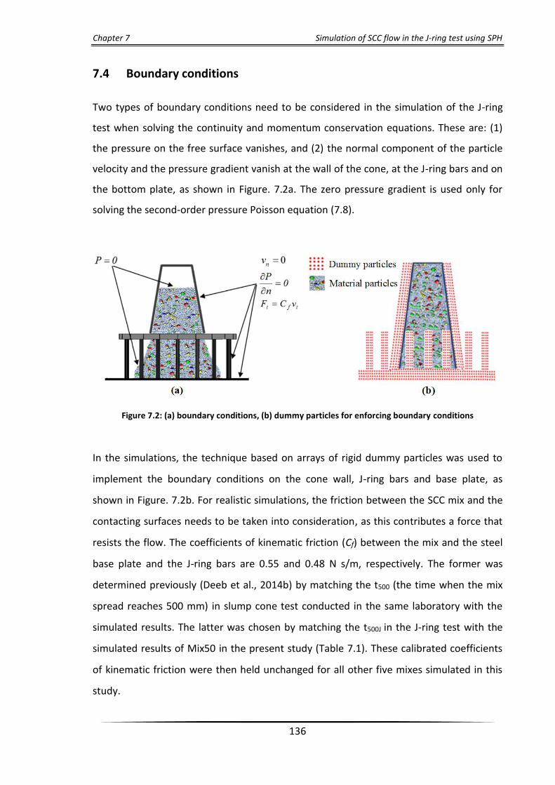
Chapter 7 Simulation of SCC flow in the J-ring test using SPH
136
7.4 Boundary conditions
Two types of boundary conditions need to be considered in the simulation of the J-ring
test when solving the continuity and momentum conservation equations. These are: (1)
the pressure on the free surface vanishes, and (2) the normal component of the particle
velocity and the pressure gradient vanish at the wall of the cone, at the J-ring bars and on
the bottom plate, as shown in Figure. 7.2a. The zero pressure gradient is used only for
solving the second-order pressure Poisson equation (7.8).
Figure 7.2: (a) boundary conditions, (b) dummy particles for enforcing boundary conditions
In the simulations, the technique based on arrays of rigid dummy particles was used to
implement the boundary conditions on the cone wall, J-ring bars and base plate, as
shown in Figure. 7.2b. For realistic simulations, the friction between the SCC mix and the
contacting surfaces needs to be taken into consideration, as this contributes a force that
resists the flow. The coefficients of kinematic friction (Cf) between the mix and the steel
base plate and the J-ring bars are 0.55 and 0.48 N s/m, respectively. The former was
determined previously (Deeb et al., 2014b) by matching the t500 (the time when the mix
spread reaches 500 mm) in slump cone test conducted in the same laboratory with the
simulated results. The latter was chosen by matching the t500J in the J-ring test with the
simulated results of Mix50 in the present study (Table 7.1). These calibrated coefficients
of kinematic friction were then held unchanged for all other five mixes simulated in this
study.

Chapter 7 Simulation of SCC flow in the J-ring test using SPH
137
Table 7. 1: Simulation trials on Mix50 to determine the coefficients of kinematic friction (Cf) between the
mix and the steel of J-ring bars
Mix designation
Plastic viscosity, Pa s
Yield stress, Pa
Trial Cf t500J
experimental, s t500J
simulated, s
Mix50A 7.84 180
0.44
1.4
1.3
0.46 1.3
0.48 1.4
7.5 Treatment of particles in the simulated mixes
The volume of the mix in the cone, 5.498 × 106 mm3, was simulated by 23,581 particles. If
all particles possess the same density as the viscous homogeneous continuum, the
number of particles used gives a resolution of 233.15 mm3 per particle. This resolution
will be rather different if the particles possess different densities, and therefore, the large
aggregates that can be distinguished from the homogeneous mass must have a volume
exceeding this minimum. That is why only the aggregates of size 8 mm and above could
be treated as discrete identities.
The simulated particles were generated randomly. Particles representing the mortar as
well as the coarse aggregates form a homogeneous mass and possess the same
continuum properties except for their assigned volumes. The masses of the SPH particles
representing different coarse aggregate size particles in the mix were calculated
according to their respective volume fractions in the mix. The volume fractions of coarse
aggregates in different size ranges (g ≥ 20, 16 ≤ g < 20, 12 ≤ g < 16 and 8 ≤ g < 12 mm)
were calculated (Table 7.2) by performing sieve analysis within a given aggregate test
sample. For the purpose of modelling, each aggregate size range was replaced by a
representative aggregate size, as illustrated in Table 7.2. Also given in Table 7.2 is the
assigned volume (Va) for each particle size, which appears in the discrete form of SPH
equations is equal to the ratio of its actual mass to the density of the continuum. The
calculation of the assigned volumes of particles corresponding to their size range (g) in
the 3D simulation of J-ring test is presented in the following section.
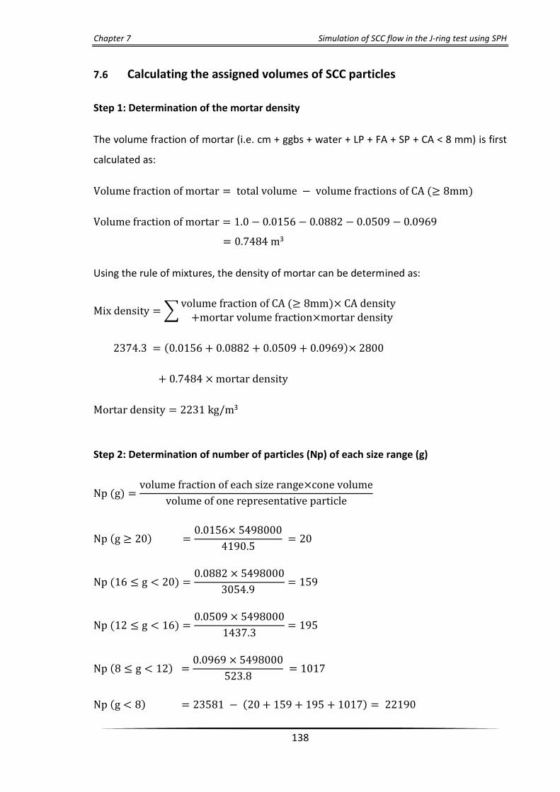
Chapter 7 Simulation of SCC flow in the J-ring test using SPH
138
7.6 Calculating the assigned volumes of SCC particles
Step 1: Determination of the mortar density
The volume fraction of mortar (i.e. cm + ggbs + water + LP + FA + SP + CA < 8 mm) is first
calculated as:
Volume fraction of mortar = total volume − volume fractions of CA (≥ 8mm)
Volume fraction of mortar = 1.0 − 0.0156 − 0.0882 − 0.0509 − 0.0969
= 0.7484 m3
Using the rule of mixtures, the density of mortar can be determined as:
Mix density =∑volume fraction of CA (≥ 8mm)× CA density +mortar volume fraction×mortar density
2374.3 = (0.0156 + 0.0882 + 0.0509 + 0.0969)× 2800
+ 0.7484 × mortar density
Mortar density = 2231 kg/m3
Step 2: Determination of number of particles (Np) of each size range (g)
Np (g) =volume fraction of each size range×cone volume
volume of one representative particle
Np (g ≥ 20) =0.0156× 5498000
4190.5 = 20
Np (16 ≤ g < 20) =0.0882 × 5498000
3054.9 = 159
Np (12 ≤ g < 16) =0.0509 × 5498000
1437.3= 195
Np (8 ≤ g < 12) =0.0969 × 5498000
523.8 = 1017
Np (g < 8) = 23581 − (20 + 159 + 195 + 1017) = 22190

Chapter 7 Simulation of SCC flow in the J-ring test using SPH
139
Step 3: Determination of volume of each representative mortar particle (𝐠 < 𝟖)
Volume of mortar in the cone = mortar volume fraction× cone volume
= 0.7484×5498000 = 4114703 mm3
Volume of each mortar particle (g < 8) =volume of mortar in the cone
Np(g < 8)
=4114703
22191= 185.422 mm3
Step 4: Determination of the assigned volume (Va) of each size range (g)
Assigned volume per particle (Va) =actual volume of particle×actual density
density of continuum
Va (g ≥ 20) =4190.5×2800
2374.3 = 4941.8 mm3
Va (16 ≤ g < 20) =3054.9×2800
2374.3 = 3602.6 mm3
Va (12 ≤ g < 16) =1437.3 ×2800
2374.3 = 1695.0 mm3
Va (8 ≤ g < 12) =523.8×2800
2374.3 = 617.7 mm3
Va (< 8) =185.422×2231
2374.3= 174.2 mm3

Chapter 7 Simulation of SCC flow in the J-ring test using SPH
140
Table 7. 2: Volume fractions and assigned volumes of particles corresponding to their size range (g) in the
3D simulation of J-ring test
Mix
particles
Particle
range,
mm
Representative
particle
diameter, mm
Density
kg/m3
Volume
fraction,
%
3D J-ring test
Number of
particles
Assigned volume
per particle, mm3
Agg
rega
te p
arti
cle
s g ≥ 20 20 2800 1.56 20 4941.8
16 ≤ g <20 18 2800 8.82 159 3602.6
12 ≤ g < 16 14 2800 5.09 195 1695.0
8 ≤ g < 12 10 2800 9.69 1017 617.7
Mo
rtar
par
ticl
es
g < 8 2231 74.84 22190 174.2
Total 2374.3 100 23581
Throughout the simulation, particles representing the coarse aggregates based on their
assigned volumes were tagged (Figure 7.3) in order to monitor their velocity vectors and
positions.
Figure 7.3 : Schematic sketch of particle representation in the simulated mixes (After: Deeb et al., 2014a)

Chapter 7 Simulation of SCC flow in the J-ring test using SPH
141
7.7 Simulation results
To investigate how efficient the SPH is to predict the flow of SCC mixes through gaps in
the reinforcing bars, different SCC mixes were three-dimensionally simulated in the J-ring
apparatus. The rheological parameters (plastic viscosity and yield stress) of each of these
mixes have been determined. The plastic viscosity of a mix was calculated using the
micromechanical procedure described in (Ghanbari and Karihaloo, 2009), based on the
plastic viscosity of the paste (i.e. cement, ggbs, water, super-plasticiser and entrapped
air). The latter was estimated from viscometer measurements of similar pastes reported
in the literature (Sun et al., 2006; Nehdi and Rahman, 2004). The results are given in Table
7.3. The yield stress (𝜏𝑦) was predicted in an inverse manner using the SPH simulation of
slump flow test (Badry et al., 2016). Over the wide range of SCC mixes (30 – 80 MPa)
simulated, it has been found (Badry et al., 2016) that the τy varies only marginally from
175 to 190 Pa. Therefore, the same range was used for τy of the mixes in the present
study (Table 7.3).
The simulation and experimental results for t500J and spread of all mixes are shown in
Table 7.3. It is noted that the results are in very good agreement. It will be recalled that
only mix 50MPa was used to calibrate the coefficient of kinematic friction (Cf) between
the mix and bars, which was then held unchanged for the simulations of all the remaining
five mixes. The simulation results of SCC mixes will be discussed below in terms of flow
pattern and t500J, passing ability, and segregation resistance. In this study, it is worth
mentioning that the simulation has been performed on a narrow spacing bar J-ring test
(with 16 bars; this is the current British standard (BS EN 12350-12, 2010)) and a wide one
(with 10 bars; this was the earlier European standard, now superseded) to simulate the
SCC flow in congested and normal reinforcement, respectively. The former will be
reported in this chapter, whereas the latter is described in Appendix G.

Chapter 7 Simulation of SCC flow in the J-ring test using SPH
142
Table 7. 3: Simulation and experimental results for SCC mixes
Mix
Designation
Plastic
viscosity, Pa
s
Yield
stress,
Pa
t500J , s Spread diameter, mm
experimental simulated experimental simulated
30 4.63 175 0.7 0.7 650 640
40 6.84 175 0.8 0.9 700 680
50 7.84 180 1.4 1.4 640 640
60 8.18 175 1.5 1.6 665 655
70 9.32 180 2.0 2.0 690 695
80 10.47 190 2.8 2.7 700 700
7.7.1 Mix flow pattern and t500J
The experimental and simulated flow patterns of selected SCC mix (Mix60) at different
times during the flow are shown in Figures 7.4 – 7.6. The experimental and simulated flow
patterns of all the remaining five mixes are shown in Appendix G. The simulations are
found to be well correlated with the experimental results. From Figure 7.4 it can be
noticed that the shape and the free surface profile of the simulated mix around the J-ring
bars is similar to that observed in the test. The spread at 500 mm diameter also looks very
similar to that observed in the laboratory test (Figure 7.5). The final spread of the
simulated mix has the same smooth “pancake” appearance as in the laboratory test
(Figure 7.6). Moreover, it can be observed (Table 7.3) that SPH can predict very well the
time needed for flow to reach the spread at 500 mm diameter (t500J) for all the test mixes.

Chapter 7 Simulation of SCC flow in the J-ring test using SPH
143
Figure 7.4: Flow pattern of SCC Mix60 just after passing through the gaps in J-ring bars (at 0.5 s)
Figure 7.5: Flow pattern of SCC Mix60 at t500J (at 1.5 s)
Figure 7.6: Flow pattern of SCC Mix60 after it has stopped (at 11.0 s)

Chapter 7 Simulation of SCC flow in the J-ring test using SPH
144
7.7.2 Passing ability
With the reference to the passing ability criterion, SCC should have the ability to flow and
pass through congested reinforcement and narrow openings while maintaining adequate
suspension and distribution of coarse particles in the matrix. This means that arching near
obstacles and blockage during flow have to be avoided. In this simulation, the SCC passing
ability can be judged in terms of the height difference between the concrete inside and
outside the steel bars of the J-ring according to BS EN12350-12 (2010). Taking the
acceptance criterion of SCC passing ability that the height difference is ≤ 10 mm (BS EN
206-9, 2010), it is clear from Table 7.4 that all the six simulated mixes did flow through
the gaps in the J-ring without blockage, as indeed they did in the laboratory tests.
Table 7. 4: Height difference between the concrete inside and outside the steel bars of the J-ring test
Mix Designation Height difference, mm
experimental simulated
30A 10 10
40A 7 8
50A 10 9
60A 9 7
70A 7 7
80A 7 5
7.7.3 Assessment of segregation resistance
The numerical simulation of flow, as shown above, is a powerful tool for understanding
the rheological behaviour of SCC mixes in terms of flow pattern, t500J, the flow spread and
passing ability (i.e. no blockage). It can also be used for assessing the segregation
resistance of the SCC mix through an assessment of the coarse aggregate distribution in
the “pancake” after it has stopped to flow. For this, the distribution of coarse aggregates
in the SCC mixes will be evaluated along three different cut sections: (1) in three
concentric circular regions of the “pancake”, (2) in four quadrants and (3) along two
orthogonal diameters.

Chapter 7 Simulation of SCC flow in the J-ring test using SPH
145
In concentric regions approach the coarse aggregate distribution in the mix “pancake” has
been evaluated, following an approach proposed by Tregger et al. (2012) for experimental
slump flow “pancake”. Their assessment procedure is based on the concentration of
aggregates in concentric rings, irrespective of whether this concentration is made up of
aggregates of one or several size ranges. However, if the concentration of aggregates is
the same in all the rings, there is no guarantee that the distribution of aggregates of
different size ranges is the same. It is the distribution of coarse aggregates of different
size ranges that determines whether or not there is segregation in the mix. Therefore, the
approach proposed in (Tregger et al., 2012) has been applied here to the SCC coarse
aggregate distribution rather than its concentration in the simulated J-ring “pancake”.
The distribution has been determined in three concentric circular regions: inside the J-ring
(Figure 7.7A), between the outer edge of J-ring bars and a diameter of 500 mm spread
(Figure 7.7B), and finally between the diameter of 500 mm and the final spread of the mix
(Figure 7.7C). From Figure 7.8 it can be seen that the coarse aggregates in the three
concentric circular regions are evenly distributed throughout the matrix.
Figure 7.7 : Coarse aggregate distributions in the three concentric circular regions

Chapter 7 Simulation of SCC flow in the J-ring test using SPH
146
Figure 7.8: The three concentric circular regions to evaluate the distribution of coarse aggregates in the J-
ring “pancake”
The distributions of coarse aggregates in the SCC mix ‘’pancake” were also calculated
after splitting the “pancake” into four quadrants (Figure 7.9). In each quadrant, the
distribution was quantified by counting the number of coarse aggregate particles in each
size range. It can be seen from Figure 7.10 that the larger aggregates (≥ 8 mm) are almost
identically distributed in the four quadrants, providing further confirmation of the
segregation resistance of the mix. Thus, SPH allows tagging of the large aggregate
particles in order to track their locations during the flow and after it has stopped.
0.0
0.2
0.4
0.6
0.8
1.0
(8-12) (12-16) (16-20) (>20)
CD
F
Coarse aggregate range size, mm
Region A Region B Region C

Chapter 7 Simulation of SCC flow in the J-ring test using SPH
147
Figure 7.9: Four quadrants of Mix50 “pancake” to determine the aggregate distribution
Figure 7.10: Coarse aggregate distributions in the four quadrants
0.0
0.2
0.4
0.6
0.8
1.0
(8-12) (12-16) (16-20) (>20)
CD
F
Coarse aggregate range size, mm
Quadrant 1 Quadrant 2
Quadrant 3 Quadrant 4

Chapter 7 Simulation of SCC flow in the J-ring test using SPH
148
The coarse aggregates along the two diametrical sections (AA and BB in Figure 7.11) were
investigated by performing a statistical analysis on the coarse aggregates exposed in
these sections (Figure 7.12) using the Weibull cumulative distribution function (CDF).
Figure 7.13 confirms that the distributions of the coarse aggregate particles of different
size ranges are nearly the same along the cut diameters. This attests to the homogeneity
of flow, i.e. to no segregation during the flow. Therefore, the numerical methodology
(SPH) can capture the flow behaviour of SCC mixes and provide insight into the
distribution of large aggregates during the flow.
Figure 7.11: Flow pattern of SCC (Mix30) showing the large aggregates
Figure 7.12: Coarse aggregate distributions along diametrical cross-sections (AA and BB) of Mix30
“pancake”
AA
A
BB
AA
BB

Chapter 7 Simulation of SCC flow in the J-ring test using SPH
149
Figure 7.13: Coarse aggregate distributions along the diametrical cross-sections
7.8 Remarks on simulation time
In the above numerical strategy, the SCC incompressibility has been imposed exactly
through the pressure Poisson equation (7.8). This is found to be very time-consuming. An
alternative strategy that is very popular in many applications was therefore also tried. In
this strategy the incompressibility condition is imposed approximately through the so-
called weakly or quasi-compressible SPH (Monaghan, 1994). It leads to the replacement
of the real incompressible fluid by an artificial quasi-compressible fluid having a small,
user-defined, fluctuation in the density. However, it requires a much smaller time step in
order to keep the density fluctuation down to 1% (Lee et al., 2008). The weakly
incompressible SPH strategy was implemented on one SCC mix (Mix50) in order to check
whether or not it leads to a significant reduction in the simulation time in comparison
with the method used above. The simulations (in 10-bar J-ring test), for both weakly-
compressible SPH (WCSPH) and incompressible SPH (ISPH), were simultaneously run on
STONE PC-1210 workstation (3.60 GHz, Intel(R) Core(TM) i7-4790 CPU). It was found that
the time taken to simulate the flow for 10 s in WCSPH approximation was actually longer
0.0
0.2
0.4
0.6
0.8
1.0
(8-12) (12-16) (16-20) (>20)
CD
F
Coarse aggregate range size, mm
Section A-A Section B-B

Chapter 7 Simulation of SCC flow in the J-ring test using SPH
150
than that in ISPH, 98 h against 65 h. This is no doubt a result of the fact that the time step
in implicit WCSPH scheme had to be very small to avoid numerical instability (Lee et al.,
2008).
7.9 Concluding remarks
Smooth particle hydrodynamics (SPH), with its adaptability, simplicity and Lagrangian
nature, is more attractive approach to deal with the heterogeneous flow. In the field of
SCC, it has high potential for greater acceptance and wider applications such as, mix
proportioning, predicting the rheological parameters, modelling the flow and monitoring
the movement of large aggregates and/or short steel fibres in the cone slump flow and L-
box tests. In this chapter, the goal was to extend the SPH approach to simulating the flow
of SCC through gaps in reinforcing bars using the J-ring test. In this test the capabilities of
SPH methodology were validated by comparing the experimental and simulations results
of different SCC mixes. The comparison showed that the simulations were in very good
agreement with experimental results for all six mixes. The free surface profiles around the
J-ring bars, the spread at 500 mm diameter and the final flow pattern are all captured
accurately by SPH.
In this simulation, the SCC passing ability was judged in terms of the height difference
between the concrete inside and outside the steel bars of the J-ring. The results showed
that all the six simulated mixes did flow through the gaps in the J-ring without blockage,
as indeed they did in the laboratory tests. In term of segregation resistance aassessment,
SPH allows tagging of the large aggregate particles in order to track their locations during
the flow and after it has stopped. This allows the distribution of large aggregates in the
mixes to be examined in order to ensure that they have not segregated from the mortar.
The SPH simulation methodology can indeed replace the time-consuming laboratory J-
ring test, thereby saving time, effort and materials.
Regarding the numerical solution strategies used in SPH, it is revealed that there is no
advantage to be gained in terms of simulation time by approximating the truly
incompressible SCC by a weakly incompressible SCC at least on the computational
platform used in this study.

Conclusions and recommendations for
further study

Chapter 8 Conclusions and recommendations for further study
152
8.1 Conclusions
From the main achievements of the research work embodied in this thesis, the following
conclusions can be drawn:
❖ Self-compacting concrete (SCC) has undergone extensive investigations that have led
to confidence in its fresh and hardened properties. Nevertheless, its mix
proportioning methods have not kept pace with their production techniques. An
easy-to-use rational method for designing an SCC mix based on the desired target
plastic viscosity and compressive strength of the mix was developed in the present
study. The systematic steps taken to develop this rational method were described in
Chapter 4. It is based on the micromechanical procedure that has recently been
developed to determine the SCC mix plastic viscosity. It should not be forgotten that
the developed micromechanical procedure has enriched this research work far
beyond the scope of its original intended use for the determination of SCC mix plastic
viscosity; it forms the backbone of this rational mix design method. The simplicity and
usefulness of this mix proportioning method are enhanced by the provision of design
charts as a guide for mix proportioning. The characteristic cube strength of mixes
varied between 30 and 80 MPa at 28 days age, and the target plastic viscosity
between 3 and 15 Pa s: the upper bound of all mix grades was 15 Pa s, whereas the
lower bound varied between 3 – 8 Pa s in mix grade range 30 – 80 MPa.
❖ The experimental work attesting the validity of the proposed mix design procedure
was performed via a series of SCC mixes in both fresh and hardened states (Chapter
5). The test mixes were found to meet the necessary self-compacting and the
compressive strength criteria, thus fully validating the proposed mix proportioning
method. Therefore, this method reduces considerably the extent of laboratory work,
the testing time and the materials used. Enhancing the sustainability of the designed
SCC mixes, the coarser fraction of limestone filler was successfully used to replace an
equivalent volume of river sand fine aggregate. Such a replacement is
environmentally friendly and economic.
❖ Although SCC has left his early stage of laboratory studies and has now become an
industrial product, the differences in its composition from VC sill raise concerns about
its fracture behaviour. The concern is primarily because a lower coarse aggregate

Chapter 8 Conclusions and recommendations for further study
153
content in an SCC mix relative to a VC mix of the same grade is likely to reduce its
energy absorption capacity and thus its ductility. In this study, the role of several
composition parameters of SCC mixes (coarse aggregate (CA) volume, paste to solids
ratio (p/s) and water to binder ratio (w/cm)) in their fracture behaviour was
investigated (Chapter 6). The results showed that the specific fracture energy
(𝐺𝐹) increases with an increase in the CA volume fraction, irrespective of the SCC mix
grade, although the increase is less pronounced in higher strength than in low
strength SCC mixes. Within the same nominal strength grade, an increase in the p/s
results in a marginal increase in the strength itself, but a noticeable decrease in 𝐺𝐹.
Besides that, an increase in the w/cm ratio reduces 𝐺𝐹. The decrease becomes more
pronounced with decreasing CA volume fraction.
❖ The critical crack opening (𝑤𝑐) of the test notched beams is dominated by the CA
volume in the mix and the mix grade. The larger the CA volume (or the smaller the
p/s) the larger is the critical crack opening (𝑤𝑐). However, the higher the mix grade
the lower is the 𝑤𝑐. As in 𝑤𝑐, the same tendency was found in the characteristic
length (𝑙𝑐ℎ), which is also dominated by the CA volume fraction and strength grade.
Also investigated in this study is the relationship between the direct tensile strength
(determined by the inverse analysis using the non-linear hinge model) and splitting
strength (𝑓𝑐𝑡/𝑓𝑠𝑡) of SCC mixes of different p/s ratio and mix grade. It is found that
𝑓𝑐𝑡/𝑓𝑠𝑡 is dominated by the p/s in the mix and the mix grade: it increases with both an
increase in p/s and mix grade.
❖ An incompressible mesh-less smooth particle hydrodynamics (SPH) methodology has
been implemented to simulate the flow of SCC through gaps in reinforcing bars using
the J-ring test. A suitable Bingham-type constitutive model has been coupled with the
Lagrangian momentum and continuity equations to simulate the flow. The
capabilities of SPH methodology were validated by comparing the experimental and
simulations results of different SCC mixes (Chapter 7). The comparison showed that
the simulations were in very good agreement with experimental results for all the
test mixes. The free surface profiles around the J-ring bars, the spread at 500 mm
diameter and the final flow pattern are all captured accurately by SPH.

Chapter 8 Conclusions and recommendations for further study
154
❖ The results also showed that all the simulated mixes did flow through the gaps in the
J-ring without blockage, as indeed they did in the laboratory tests. In terms of
segregation assessment, SPH allows tagging of the large aggregate particles in order
to track their locations during the flow and after it has stopped. This allows the
distribution of large aggregates in the mixes to be examined in order to ensure that
they have not segregated from the mortar. The SPH simulation methodology can
indeed replace the time-consuming laboratory J-ring test, thereby saving time, effort
and materials.
❖ With respect to the numerical solution strategies used in SPH, it was revealed that
there is no advantage to be gained in terms of simulation time by approximating the
truly incompressible SCC by a weakly incompressible SCC at least on the
computational platform used in this study.
8.2 Recommendations for further study
The development of SCC has revolutionised construction processes by offering superior
economic and technical advantages over VC. Being one of the future environmentally-
friendly materials for buildings and different construction applications, further research in
SCC is worthwhile, and the following areas are recommended for future study:
❖ It would be interesting to construct design charts for proportioning SCC mixes whose
plastic viscosity is below the lower limit of 3 Pa s and above the upper limit of 15 Pa s.
The former could be achieved by adding a high level of cement replacement
materials (e.g. ggbs) and/or high dosage of super-plasticisers. The latter, however,
could be attained by adding a viscosity modifying agent (VMA).
❖ All the design charts of the proposed mix design procedure, reported in Chapter 4,
were developed for proportioning SCC mixes without fibres, and with the
characteristic cube strength between 30 and 80 MPa. The procedure can, of course,
be generalised, and the design charts be enriched if steel fibres are used and the
range of characteristic cube strengths is extended.

Chapter 8 Conclusions and recommendations for further study
155
❖ It would be advisable to investigate the role of compositional parameters (p/s, CA
volume and w/cm) of SCC mixes, with or without steel fibres, in their fracture
behaviour using lightweight aggregate instead of normal aggregate. This could give a
clearer picture of the fracture behaviour of the lightweight concrete in terms of
specific fracture energy, the critical crack opening and the mix ductility.
❖ To exploit the full potential of SPH approach, the flow of SCC mixes and monitoring of
their coarse aggregate is worthwhile to be simulated into practical size formworks
with the presence of different sizes and densities of reinforcement. To gain this
advantage, it is, however, necessary to accelerate the SPH simulation process, as
time taken to simulate the flow will be longer than that in the standard tests.

References

References
157
Abdalla, H.M. and Karihaloo, B.L. (2003). Determination of size-independent specific
fracture energy of concrete from three-point bend and wedge splitting tests. Magazine of
Concrete Research, 55(2), pp. 133–141.
Abdalla, H.M. and Karihaloo, B.L. (2004). A method for constructing the bilinear tension
softening diagram of concrete corresponding to its true fracture energy. Magazine of
Concrete Research, 56(10), pp. 597–604.
Abo Dhaheer, M.S., Al-Rubaye, M.M., Alyhya, W.S., Karihaloo, B.L. and Kulasegaram, S.
(2016a). Proportioning of self-compacting concrete mixes based on target plastic viscosity
and compressive strength: experimental validation. Journal of Sustainable Cement-Based
Materials, 5(4), pp. 217–232.
Abo Dhaheer, M.S., Al-Rubaye, M.M., Alyhya, W.S., Karihaloo, B.L. and Kulasegaram, S.
(2016b). Proportioning of self–compacting concrete mixes based on target plastic
viscosity and compressive strength: mix design procedure. Journal of Sustainable Cement-
Based Materials, 5(4), pp. 199–216.
ACI Committee 211. (1991). Standard practice for selecting proportions for normal, heavy
weight and mass concrete. Manual of Concrete Practice (reapproved), pp. 1–38.
Akçaoǧlu, T., Tokyay, M. and Çelik, T. (2004). Effect of coarse aggregate size and matrix
quality on ITZ and failure behavior of concrete under uniaxial compression. Cement and
Concrete Composites, 26, pp. 633–638.
Akcay, B., Agar-Ozbek, A.S., Bayramov, F., Atahan, H.N., Sengul, C. and Tasdemir, M.A.
(2012). Interpretation of aggregate volume fraction effects on fracture behavior of
concrete. Construction and Building Materials, 28(1), pp. 437–443.
Al-Rubaye, M.M. 2016. Self-compacting concrete: design, properties and simulation of
the flow characteristics in the L-box. PhD thesis, School of Engineering, Cardiff University,
UK.
Alyhya, W.S. 2016. Self-compacting concrete: mix proportioning, properties and its flow
simulation in the V-funnel. PhD thesis, School of Engineering, Cardiff University, UK.

References
158
Amini, Y., Emdad, H. and Farid, M. (2011). A new model to solve fluidhypo-elastic solid
interaction using the smoothed particle hydrodynamics (SPH) method. European Journal
of Mechanics, B/Fluids 30(2), pp. 184–194.
Assaad, J., Khayat, K., Mesbah, H. (2003). Assessment of the thixotropy of flowable and
self-consolidating concrete. ACI Materials Journal, 100(2), pp. 99–107.
ASTM C1621/C1621M. 2008. Standard test method for passing ability of self-
consolidating concrete by J-ring.
Baaijens, F.P.T. (2001). A fictitious domain/mortar element method for fluid-structure
interaction. International journal of numerical methods in fluids, 35, pp. 743–761.
Badry, F., Kulasegaram, S. and Karihaloo, B.L. (2016). Estimation of the yield stress and
distribution of large aggregates from slump flow test of self-compacting concrete mixes
using smooth particle hydrodynamics simulation. Journal of Sustainable Cement-Based
Materials, 5(3), pp. 117–134.
Badry, F.F. (2015). Experimental and numerical studies in self-compacting concrete. PhD
thesis, School of Engineering, Cardiff Unversity, UK.
Banfill, P., Beaupr, D., Chapdelaine, F., de Larrard, F., Domone, P., Nachbaur, L. (2000).
Comparison of concrete rheometers: International tests at LCPC. Ferraris, C. F. and
Brower, L. E. ed. National Institute of Standards and Technology, Nantes, France.
Banfill, P.F. (2006). Rheology of fresh cement and concrete. Rheology Reviews, pp. 61–
130.
BASF. (2014). MasterGlenium ACE 499: High range water reducing admixture for
concrete.
Bažant, Z.P. (1984). Size effect in blunt fracture: concrete, rock, metal. ASCE Journal of
Engineering Mechanics, 110, pp. 518-535.
Bažant, Z.P. (1996). Analysis of work-of-fracture method for measuring fracture energy of
concrete. Journal of Engineering Mechanics 122, pp. 138–144.

References
159
Bažant, Z.P. and Kazemi, M.T. (1991). Size dependence of concrete fracture energy
determined by RILEM work-of-fracture method. International Journal of Fracture, 51(2),
pp. 121–138.
Bažant, Z.P. and Planas, J. (1997). Fracture and size effect in concrete and other quasi-
brittle materials. UK: CRC Press.
Becker, M., Teschner, M. (2007). Weakly compressible SPH for free surface flows. San
Diego, Eurographics/ ACM SIGGRAPH Symposium on Computer Animation, pp. 1-8.
Beygi, M., Kazemi, M.T., Amiri, J. V., Nikbin, I.M., Rabbanifar, S. and Rahmani, E. (2014a).
Evaluation of the effect of maximum aggregate size on fracture behavior of self
compacting concrete. Construction and Building Materials, 55, pp. 202–211.
Beygi, M., Kazemi, M.T., Nikbin, I.M. and Amiri, V.J. (2013a). The effect of water to
cement ratio on fracture parameters and brittleness of self-compacting concrete.
Materials and Design, 50, pp. 267–276.
Beygi, M., Kazemi, M.T., Nikbin, I.M. and Amiri, V.J. (2014b). The effect of aging on the
fracture characteristics and ductility of self-compacting concrete. Materials and Design,
55, pp. 937–948.
Beygi, M., Kazemi, M.T., Nikbin, I.M., Amiri, V.J., Rabbanifar, S. and Rahmani, E. (2014c).
The influence of coarse aggregate size and volume on the fracture behavior and
brittleness of self-compacting concrete. Cement and Concrete Research, 66, pp. 75–90.
Beygi, M.H., Berenjian, J., Lotfi Omran, O., Sadeghi Nik, A. and Nikbin, I.M. (2013b). An
experimental survey on combined effects of fibers and nanosilica on the mechanical,
rheological, and durability properties of self-compacting concrete. Materials and Design,
50, pp. 1019–1029.
Bonet, J., Kulasegaram, S., (2000). Correction and stabilization of smooth particle
hydrodynamic methods with application in metal forming simulations. International
Journal of Numerical Methods in Engineering, 47(6), pp. 1189-1214.

References
160
Bonet, J., Lok, T. S. L., (1999). Variational and momentum aspects of smooth particle
hydrodynamics formulations. Computer Method in Applied Mechanics and Engineering,
180(1-2), pp. 97-115.
Bosiljkov, V.B. (2003). SCC mixes with poorly graded aggregate and high volume of
limestone filler. Cement and Concrete Research, 33(9), pp. 1279–1286.
Boukendakdji, O., Kadri, E. and Kenai, S. (2012). Effects of granulated blast furnace slag
and super-plasticizer type on the fresh properties and compressive strength of self-
compacting concrete. Cement and Concrete Composites, 34(4), pp. 583–590.
Brouwers, H. J. H., Radix, H. J. (2005). Self-Compacting Concrete: Theoretical and
experimental study. Cement and Concrete Research, 35 (11), pp. 2116–2136.
BS 1881. (1983). Part 121. Method for determination of static modulus of elasticity in
compression. British Standards publication.
BS EN 12350-10. (2010). Testing fresh concrete, Part 10: Self-compacting concrete - L-box
test. British Standards publication.
BS EN 12350-8. (2010). Testing fresh concrete, Part 8: Self-compacting concrete - Slump
flow test. British Standards publication.
BS EN 12350-9. (2010). Testing fresh concrete, Part 9: Self-compacting concrete - V-
funnel test. British Standards publication.
BS EN 12350-12. (2010). Testing fresh concrete, Part 9: Self-compacting concrete - J- ring
test. British Standards publication.
BS EN 12390. (2009). Part 3. Testing hardened concrete: Compressive strength of test
specimens. British Standards publication.
BS EN 12390. (2009). Part 6. Testing hardened concrete: Tensile splitting strength of test
specimens. British Standards publication.

References
161
BS EN 197. (2011). Part 1. Cement: Composition, specifications and conformity criteria for
common cements. British Standards publication.
BS EN 206-9. (2010). Additional Rules for Self-compacting concrete (SCC). British
Standards publication.
Bui, V.K., Akkaya, Y. and Shah, S.P. (2002). Rheological model for self-consolidating
concrete. ACI Materials Journal, 99(6), pp. 549–559.
Carpinteri, A. and Brighenti, R. (2010). Fracture behaviour of plain and fiber-reinforced
concrete with different water content under mixed mode loading. Materials and Design,
31(4), pp. 2032–2042.
Carpinteri, A. and Chiaia, B. (1996). Size effects on concrete fracture energy: dimensional
transition from order to disorder. Materials and Structures, 29(5), pp. 259–266.
Chidiac, S.E. and Mahmoodzadeh, F. (2009). Plastic viscosity of fresh concrete- A critical
review of predictions methods. Cement and Concrete Composites, 31(8), pp. 535–544.
Choi, Y.W., Kim, Y.J., Shin, H.C. and Moon, H.U. (2006). An experimental research on the
fluidity and mechanical properties of high-strength lightweight self-compacting concrete.
Cement and Concrete Research, 36(9), pp. 1595–1602.
Chorin, A.J. (1968). Numerical solution of the Navier-Stokes equations. Mathematics of
Computation, 22(104), pp. 745–762.
Cifuentes, H. and Karihaloo, B.L. (2013). Determination of size-independent specific
fracture energy of normal and high strength self-compacting concrete from wedge
splitting tests. Construction and Building Materials, 48(2), pp. 548–553.
Collepardi, M., Collepardi, S. and Troli, R. (2007). Properties of SCC and flowing concrete.
In: Kraus, R. N., Naik, T. R. and Pouya, P. ed. Proceeding International Conference:
Sustainable Construction Materials and Technologies. Coventry, UK: Special papers
proceedings, UW Milwaukee CBU, pp. 25–31.
Corinaldesi, V. and Moriconi, G. (2004). Durable fiber reinforced self-compacting
concrete. Cement and Concrete Research, 34(2), pp. 249–254.

References
162
Craeye, B., Itterbeeck, P.V., Desnerck, P., Boel, V. and De Schutter, G. (2014). Modulus of
elasticity and tensile strength of self-compacting concrete: survey of experimental data
and structural design codes. Cement and Concrete Composites, 54, pp. 53–61.
Cummins, S.J. and Rudman, M. (1999). An SPH projection method. Journal of
Computational Physics, 152(2), pp. 584–607.
de Kruif, C.G., Van Iersel, E.M.F., Vrij, A. and Russel W. B. (1985). Hard sphere colloidal
dispersions: Viscosity as a function of shear rate and volume fraction. The Journal of
Chemical Physics, 83(9), pp. 4717–4725.
Deeb, R. (2013). Flow of self-compacting concrete. PhD thesis, School of Engineering,
Cardiff University, UK.
Deeb, R. and Karihaloo, B.L. (2013). Mix proportioning of self-compacting normal and
high-strength concretes. Magazine of Concrete Research, 65(9), pp. 546–556.
Deeb, R., Karihaloo, B.L., Kulasegaram, S. (2014a). Reorientation of short steel fibres
during the flow of self-compacting concrete mix and determination of the fibre
orientation factor. Cement and Concrete Research, 56, pp. 112–120.
Deeb, R., Kulasegaram, S. and Karihaloo, B.L. (2014b). 3D modelling of the flow of self-
compacting concrete with or without steel fibres. Part I: slump flow test. Computational
Particle Mechanics, 1, pp. 373–389.
Deeb, R., Kulasegaram, S. and Karihaloo, B.L. (2014c). 3D modelling of the flow of self-
compacting concrete with or without steel fibres. Part II: L-box test and the assessment of
fibre reorientation during the flow. Computational Particle Mechanics, 1, pp. 391–408.
Desnerck, P., Boel, V., Craeye, B. and Itterbeeck, P.V. (2014). Mechanical properties of
self-compacting concrete. In: K. H. Khayat and G. De Schutter ed. Self-Compacting
Concrete - State-of-the-Art Report of RILEM. RILEM Publications SARL, pp. 15–72.
Dinakar, P., Babu, K.G. and Santhanam, M. (2008). Durability properties of high volume fly
ash self compacting concretes. Cement and Concrete Composites, 30(10), pp. 880–886.

References
163
Dinakar, P., Reddy, M.K. and Sharma, M. (2013a). Behaviour of self-compacting concrete
using Portland pozzolana cement with different levels of fly ash. Materials and Design, 46,
pp. 609–616.
Dinakar, P., Sethy, K.P. and Sahoo, U.C. (2013b). Design of self-compacting concrete with
ground granulated blast furnace slag. Materials and Design, 43, pp. 161–169.
Domone, P.L. (2000). Mix design. In: Å. Skarendahl and Ö Petersson ed. Self-Compacting
Concrete - State-of-the-Art Report of RILEM TC 174-SCC. RILEM Publications SARL, France,
pp. 49–65.
Domone, P.L. (2003). Fresh concrete: Advanced concrete technology. In: J. Newman, B. S.
Choo ed. Elsevier Ltd.
Domone, P.L. (2006). Self-compacting concrete: An analysis of 11 years of case studies.
Cement and Concrete Composites, 28(2), pp. 197–208.
Domone, P.L. (2007). A review of the hardened mechanical properties of self-compacting
concrete. Cement and Concrete Composites, 29(1), pp. 1–12.
Domone, P.L. and Illston, J. (2010). Construction materials: Their nature and behaviour.
New York, USA: Spon Press.
Dransfield, J. (2003). Admixtures for concrete, mortar, and grout. In: Newman, J. and
Choo, B. S. ed. In Advanced Concrete Technology. USA: Elsevier Ltd.
Duan, K., Hu, X. and Wittmann, F.H. (2003). Boundary effect on concrete fracture and
non-constant fracture energy distribution. Engineering Fracture Mechanics, 70(16), pp.
2257–2268.
Duan, K., Hu, X. and Wittmann, F.H. (2007). Size effect on specific fracture energy of
concrete. Engineering Fracture Mechanics, 74, pp. 87–96.
Edamatsu, Y., Nishida, N. and Ouchi, M. (1998). A rational mix design method for self-
compacting concrete interaction between coarse aggregate and mortar particles. In: Å.
Skarendahl and Ö. Pettersson ed. 1st International RILEM Symposium on Self-Compacting

References
164
Concrete. RILEM Publications SARL, Stockholm, Sweden, pp. 309–320.EFNARC Guidelines.
2002. Specification and Guidelines for Self-Compacting Concrete. p. 32.
EFNARC Guidelines. (2005). The European Guidelines for Self-Compacting Concrete;
Specification, Production and Use. p. 63.
Felekoǧlu, B., Türkel, S. and Baradan, B. (2007). Effect of water/cement ratio on the fresh
and hardened properties of self-compacting concrete. Building and Environment, 42(4),
pp. 1795–1802.
Ferrara, L., Park, Y.D. and Shah, S.P. (2007). A method for mix-design of fiber-reinforced
self-compacting concrete. Cement and Concrete Research, 37(6), pp. 957–971.
Ferraris, C.F. (1999). Measurement of the rheological properties of high performance
concrete: State of the art report. Journal of Research of the National Institute of
Standards and Technology, 104(5), pp. 461–478.
Feys, D., Heirman, G., Schutter, G. De, Verhoeven, R., Vandewalle, L. and Gemert, D. Van
(2007). Comparison of two concrete rheometers for shear thickening behaviour of SCC.
In: G. De Schutter and V. Boel ed. 5th International RILEM Symposium on Self-Compacting
Concrete. RILEM Publications SARL, Ghent, Belgium, pp. 365–370.
Figueiras, H., Nunes, S., Coutinho, J.S. and Andrade, C. (2014). Linking fresh and durability
properties of paste to SCC mortar. Cement and Concrete Composites, 45, pp. 209–226.
Ghanbari, A. and Karihaloo, B.L. (2009). Prediction of the plastic viscosity of self-
compacting steel fibre reinforced concrete. Cement and Concrete Research, 39(12), pp.
1209–1216.
Ghanbari, A. (2011). Self-compacting high and ultra-high performance concretes. PhD
thesis, School of Engineering, Cardiff University, UK.
Ghazi, F.K. and AlJadiri, R.S. (2010). New method for proportioning self-consolidating
concrete based on compressive strength requirements. ACI Material Journal, 107(5), pp.
490-497.

References
165
Gingold, R.A. and Monaghan, J.J. (1977). Smoothed particle hydrodynamics: theory and
application to non-spherical stars. Monthly Notices of the Royal Astronomical Society,
181(3), pp. 375–389.
Goodier, C.I. (2003). Development of self-compacting concrete. In: Proceedings of the ICE-
Structures and Buildings, 156(4), pp. 405–414.
Gram, A. and Silfwerbrand, J. (2011). Numerical simulation of fresh SCC flow: applications.
Materials and Structures, 44(4), pp. 805–813.
Guinea, G.V., Planas, J. and Elices, M. (1992). Measurement of the fracture energy using
three-point bend tests: Part 1-Influence of experimental procedures. Materials and
Structures, 25(4), pp. 212–218.
Guinea, G.V., Planas, J. and Elices, M. (1994). A general bilinear fit for the softening curve
of concrete. Materials and Structures, 27(2), pp. 99–105.
Heirman, G., Hendrickx, R., Vandewalle, L., Van Gemert, D., Feys, D., De Schutter, G.
(2009). Integration approach of the Couette inverse problem of powder type self-
compacting concrete in a wide-gap concentric cylinder rheometer: Part II. Influence of
mineral additions and chemical admixtures on the shear thickening flow behaviour.
Cement and Concrete Research 39(3), pp. 171–181.
Heirman, G., Vandewalle, L., Van Gemert, D., Wallevik, Ó. (2008). Integration approach of
the Couette inverse problem of powder type self-compacting concrete in a wide-gap
concentric cylinder rheometer. Journal of Non-Newtonian Fluid Mechanics,150(2/3), pp.
93-103.
Hillerborg, A., Modeer, M. and Petersson, P.E. (1976). Analysis of crack formation and
crack growth in concrete by means of fracture mechanics and finite elements. Cement
and Concrete Research, 6, pp. 773–782.
Hoffmann, C. and Leemann, A. (2005). Properties of self-compacting and conventional
concrete – differences and similarities. Magazine of Concrete Research, 57(6), pp. 315–
319.

References
166
Hu, X. and Duan, K. (2004). Influence of fracture process zone height on fracture energy of
concrete. Cement and Concrete Research, 34(8), pp. 1321–1330.
Hu, X. and Wittmann, F. (1992). Fracture energy and fracture process zone. Materials and
Structures, 25(6), pp. 319–326.
Hu, X. and Wittmann, F. (2000). Size effect on toughness induced by crack close to free
surface. Engineering Fracture Mechanics, 65, pp. 209–221.
Karihaloo, B.L. (1995). Fracture Mechanics and Structural Concrete. UK: Addison Wesley
Longman.
Karihaloo, B.L. and Ghanbari, A. (2012). Mix proportioning of self-compacting high and
ultra high performance concretes with and without steel fibres. Magazine of Concrete
Research, 64(12), pp. 1089–1100.
Karihaloo, B.L., Abdalla, H.M. and Imjai, T. (2003). A simple method for determining the
true specific fracture energy of concrete. Magazine of Concrete Research, 55(5), pp. 471–
481.
Karihaloo, B.L., Murthy, A.R. and Iyer, N.R. (2013). Determination of size-independent
specific fracture energy of concrete mixes by the tri-linear model. Cement and Concrete
Research, 49, pp. 82–88.
Kasemchaisiri, R. and Tangtermsirikul, S. (2008). Deformability prediction model for self-
compacting concrete. Magazine of Concrete Research, 60(2), pp. 93–108.
Khaloo, A., Raisi, E.M., Hosseini, P. and Tahsiri, H. (2014). Mechanical performance of self-
compacting concrete reinforced with steel fibers. Construction and Building Materials, 51,
pp. 179–186.
Khayat, K.H. (1998). Use of viscosity modifying admixture to reduce top-bar effect of
anchored bars cast with fluid concrete. ACI Materials Journal 95(2), pp. 158–167.
Khayat, K.H. (1999). Workability, testing, and performance of self-consolidating concrete.
ACI Materials Journal, 96(3), pp. 346–353.

References
167
Khayat, K.H. (2000). Optimization and performance of air-entrained, self-consolidating
concrete. ACI Structural Journal, 97(5), pp. 526–535.
Khayat, K.H., Ghezal, A. and Hadriche, M.S. (1999). Factorial design model for
proportioning self-consolidating concrete. Materials and Structures, 32(9), pp. 679–686.
Khayat, K.H., Hu, C. and Monty, H. (1999). Stability of self-consolidating concrete,
advantages, and potential applications. In: Å. Skarendahl and Ö. Pettersson ed. 1st
International RILEM Symposium on Self-Compacting Concrete. RILEM Publications SARL,
Stockholm, Sweden, pp. 143–152.
Kim, J.H., Noemi, N. and Shah, S.P. (2012). Effect of powder materials on the rheology and
formwork pressure of self-consolidating concrete. Cement and Concrete Composites,
34(6), pp. 746–753.
Koehler, E.P. and Fowler, D.W. (2007). Aggregates in self- consolidating concrete.
International Center for Aggregates Research (ICAR), The University of Texas, Austin, USA.
Koshizuka, S., Nobe, A. and Oka, Y. (1998). Numerical analysis of breaking waves using the
moving particle semi-implicit method. International Journal for Numerical Methods in
Fluids, 26(7), pp. 751–769.
Krieger, I.M. and Dougherty, T.J. (1959). A mechanism for Non-Newtonian flow in
suspensions of rigid spheres. Transactions of The Society of Rheology, 3, pp. 137–152.
Kulasegaram, S. and Karihaloo, B.L. (2013). Fibre-reinforced, self-compacting concrete
flow modelled by smooth particle hydrodynamics. Proceedings of the Institution of Civil
Engineers (ICE) - Engineering and Computational Mechanics 166(1), pp. 22–31.
Kulasegaram, S., Karihaloo, B.L. and Ghanbari, A. (2011). Modelling the flow of self-
compacting concrete. International Journal for Numerical and Analytical Methods in
Geomechanics, 35(6), pp. 713–723.

References
168
Lachemi, M., Hossain, K., Lambros, V., Bouzoubaa, N., (2003). Development of cost
effective self-consolidating concrete incorporating fly ash, slag cement, or viscosity-
modifying admixtures. ACI Materials Journal, 100(5), pp. 419-425.
Lee, E.S., Moulinec, C., Xu, R., Violeau, D., Laurence, D. and Stansby, P. (2008).
Comparisons of weakly compressible and truly incompressible algorithms for the SPH
mesh free particle method. Journal of Computational Physics, 227(18), pp. 8417–8436.
Li, L.G. and Kwan, a. K.H. (2011). Mortar design based on water film thickness.
Construction and Building Materials, 25(5), pp. 2381–2390.
Li, L.G. and Kwan, A.K.H. (2013). Concrete mix design based on water film thickness and
paste film thickness. Cement and Concrete Composites, 39, pp. 33–42.
Liu, G.R. and Liu, M.B. (2003). Smoothed Particle Hydrodynamics - A meshfree particle
method. Singapore: World Scientific Publishing Co. Pte. Ltd,.
Lucy, L.B. (1977). A numerical approach to the testing of the fission hypothesis. The
astronomical journal, 82(12), pp. 1013–1024.
Mindess, S. (1984). The effect of specimen size on the fracture energy of concrete.
Cement and concrete Research, 14(3), pp. 431–436.
Monaghan, J.J. (1994). Simulating free surface flows with SPH. Journal of Computational
Physics, 110(2), pp. 399–406.
Muralidhara, S., Prasad, B.K.R., Eskandari, H. and Karihaloo, B.L. (2010). Fracture process
zone size and true fracture energy of concrete using acoustic emission. Construction and
Building Materials, 24(4), pp. 479–486.
Muralidhara, S., Prasad, B.K.R., Karihaloo, B.L. and Singh, R.K. (2011). Size-independent
fracture energy in plain concrete beams using tri-linear model. Construction and Building
Materials, 25(7), pp. 3051–3058.

References
169
Murthy, A.R., Karihaloo, B.L., Iyer, N.R. and Prasad, B.K.R. (2013). Determination of size-
independent specific fracture energy of concrete mixes by two methods. Cement and
Concrete Research, 50, pp. 19–25.
Murthy, A.R., Karihaloo, B.L., Iyer, N.R. and Prasad, R.B.K. (2013a). Bilinear tension
softening diagrams of concrete mixes corresponding to their size-independent specific
fracture energy. Construction and Building Materials, 47, pp. 1160–1166.
Nallathambi, P., Karihaloo, B.L. and Heaton, B.S. (1984). Effect of specimen and crack
sizes, water/cement ratio and coarse aggregate texture upon fracture toughness of
concrete. Magazine of Concrete Research, 36(129), pp. 227–236.
Nallathambi, P., Karihaloo, B.L. and Heaton, B.S. (1985). Various size effects in fracture of
concrete. Cement and Concrete Research, 15(1), pp. 117–126.
Nanthagopalan, P. and Santhanam, M. (2009). Experimental investigations on the
influence of paste composition and content on the properties of self-compacting
concrete. Construction and Building Materials, 23(11), pp. 3443–3449.
Nehdi, M. and Rahman, M. A. (2004). Estimating rheological properties of cement pastes
using various rheological models for different test geometry, gap and surface friction.
Cement and Concrete Research, 34(11), pp. 1993–2007.
Nepomuceno, M., Oliveira, L. and Lopes, S.M.R. (2012). Methodology for mix design of
the mortar phase of self-compacting concrete using different mineral additions in binary
blends of powders. Construction and Building Materials, 26(1), pp. 317–326.
Neville, A.M. (1995). Properties of concrete. 4th ed. UK: Longman Scientific Group Ltd.
Nikbin, I.M., Beygi, M.H.A., Kazemi, M.T., Amiri, J. V., Rabbanifar, S., Rahmani, E. (2014a).
A comprehensive investigation into the effect of water to cement ratio and powder
content on mechanical properties of self-compacting concrete. Construction and Building
Materials, 57, pp. 69–80.
Nikbin, I.M., Beygi, M.H.A., Kazemi, M.T., Amiri, J. V., Rahmani, E., Rabbanifar, S. (2014c).
A comprehensive investigation into the effect of aging and coarse aggregate size and
volume on mechanical properties of self-compacting concrete. Construction and Building
Materials 59, pp. 199–210.

References
170
Nikbin, I.M., Beygi, M.H.A., Kazemi, M.T., Amiri, J. V., Rahmani, E., Rabbanifar, S. (2014b).
Effect of coarse aggregate volume on fracture behavior of self-compacting concrete.
Construction and Building Materials 52, pp. 137–145.
Noguchi, T., Oh, S.G. and Tomosawa, F. (1999). Rheological approach to passing ability
between reinforcing bars of self-compacting concrete. In: Å. Skarendahl and Ö. Petersson
ed. 1st International RILEM Symposium on Self-Compacting Concrete. RILEM Publications
SARL, Stockholm, Sweden, pp. 59–70.
Nunes, S. l., Oliveira, P.M., Coutinho, J.S. and Figueiras, J. (2009). Interaction diagrams to
assess SCC mortars for different cement types. Construction and Building Materials, 23(3),
pp. 1401–1412.
Nuruddin, M.F., Chang, K.Y. and Azmee, N.M. (2014). Workability and compressive
strength of ductile self-compacting concrete (DSCC) with various cement replacement
materials. Construction and Building Materials, 55, pp. 153–157.
Obla, K. H., Thomas, M., Shashiprakash, S. G., Perebatova, O., (2003). Properties of
concrete containing ultra-fine fly ash. ACI Materials Journal, 100(5), pp. 426-433.
Okamura, H. and Ouchi, M. (2003). Self-compacting concrete. Journal of advanced
concrete technology, 1(1), pp. 5–15.
Okamura, H., Ozawa, K. and Ouchi, M. (2000). Self-compacting concrete. Structural
Concrete, 1(1), pp. 3–17.
Okumara, H. and Ouchi, M. (1999). Self-compacting concrete development, present use
and future. In: Å. Skarendahl and Ö. Petersson ed. 1st International RILEM Symposium on
Self-Compacting Concrete. RILEM Publications SARL, Stockholm, Sweden, pp. 3–14.
Olesen, J.F. (2001). Fictitious crack propagation in fiber-reinforced concrete beams.
Journal of Engineering Mechanics, 127, pp. 272–280.
Omran, A. and Khayat, K. (2016). Models to predict form pressure exerted by SCC –
results of six field campaigns. In: 8th International RILEM Symposium on Self-Compacting
Concrete, Washington DC, USA, pp. 599–612.

References
171
Ouchi, M., Hinino, M., Ozawa, K. and Okamura, H. (1998). A rational mix design method
for mortar in self-compacting concrete. In: Proceedings of the Sixth East Asia-Pacific
Conference on Structural Engineering and Construction. Taipei, Taiwan, pp. 1307–1312.
Pamnani, N.J. (2014). Effect of curing techniques on mechanical properties of self-
compacting concrete. PhD thesis, Sardar Patel University, India.
Panesar, D.K. and Shindman, B. (2011). Elastic properties of self-consolidating concrete.
Construction and Building Materials, 25(8), pp. 3334–3344.
Parra, C., Valcuende, M. and Gómez, F. (2011). Splitting tensile strength and modulus of
elasticity of self-compacting concrete. Construction and Building Materials, 25(1), pp.
201–207.
Patzák, B. and Bittnar, Z. (2009). Modeling of fresh concrete flow. Computers and
Structures, 87, pp. 962–969.
Persson, B. (2001). A comparison between mechanical propel-ties of self-compacting
concrete and the corresponding properties of normal concrete. Cement and Concrete
Research, 31(2), pp. 193–198.
Petersson, Ö. and Billberg, P. (1999). Investigation on blocking of self- compacting
concrete with different maximum aggregate size and use of viscosity agent instead filler.
In: Å. Skarendahl and Ö. Petersson ed. 1st International RILEM Symposium on Self-
Compacting Concrete. RILEM Publications SARL, Stockholm, Sweden, pp. 333–344.
Petit, J.Y., Wirquin, E., Vanhove, Y. and Khayat, K. (2007). Yield stress and viscosity
equations for mortars and self-consolidating concrete. Cement and Concrete Research,
37(5), pp. 655–670.
Pettitt, A.R. (2014). Constructing a map of the Galaxy from numerical simulations and
synthetic observations. PhD thesis, University of Exeter, UK.
Planas, J., Elices, M. and Guinea, G.V. (1992). Measurement of the fracture energy using
three-point bend tests: Part 2-Influence of bulk energy dissipation. Materials and
Structures, 25(5), pp. 305–312.

References
172
Prokopski, G. and Langier, B. (2000). Effect of water/cement ratio and silica fume addition
on the fracture toughness and morphology of fractured surfaces of gravel concretes.
Cement and Concrete Research, 30(9), pp. 1427–1433.
Rabehi, M., Mezghiche, B. and Guettala, S. (2013). Correlation between initial absorption
of the cover concrete, the compressive strength and carbonation depth. Construction and
Building Materials, 45, pp. 123–129.
RILEM State-of-the-Art Reports. (2014). Simulation of fresh concrete flow. Roussel, N. and
Gram, A. ed. Netherlands: Springer Ltd.
RILEM State-of-the-Art Reports TC174. (2000). Self-compacting concrete. Å. Skarendahl
and Ö. Petersson ed. France: RILEM Publications SARL.
RILEM TCS50. (1985). Determination of the fracture energy of mortar and concrete by
means of three-point bend tests on notched beams. Materials and Structures, 18(106),
pp. 285–290.
Roussel, N. (2006b). A theoretical frame to study stability of fresh concrete. Materials and
Structures, 39(1), pp. 81–91.
Roussel, N. (2006a). Correlation between yield stress and slump: comparison between
numerical simulations and concrete rheometers results. Materials and Structures, 39(4),
pp. 501–509.
Roussel, N. (2007). Rheology of fresh concrete: from measurements to predictions of
casting processes. Materials and Structures, 40(10), pp. 1001–1012.
Roussel, N., Geiker, M.R., Dufour, F., Thrane, L.N. and Szabo, P. (2007). Computational
modeling of concrete flow: General overview. Cement and Concrete Research, 37(9), pp.
1298–1307.
Roussel, N., Lemaitre, A., Flatt, R.J. and Coussot, P. (2010). Steady state flow of cement
suspensions: A micromechanical state of the art. Cement and Concrete Research, 40(1),
pp. 77–84.

References
173
Roussel, N., Nguyen, T.L.H., Yazoghli, O. and Coussot, P. (2009). Passing ability of fresh
concrete: A probabilistic approach. Cement and Concrete Research, 39(3), pp. 227–232.
Rozière, E., Granger, S., Turcry, P. and Loukili, A. (2007). Influence of paste volume on
shrinkage cracking and fracture properties of self-compacting concrete. Cement and
Concrete Composites, 29(8), pp. 626–636.
Saak, A.W., Jennings, H.M. and Shah, S.P. (2001). New methodology for designing self-
compacting concrete. ACI Materials Journal 98(6), pp. 429–439.
Shao, S. and Lo, E.Y.M. (2003). Incompressible SPH method for simulating Newtonian and
non-Newtonian flows with a free surface. Advances in Water Resources, 26(7), pp. 787–
800.
Shi, C., Wu, Z., Lv, K. and Wu, L. (2015). A review on mixture design methods for self-
compacting concrete. Construction and Building Materials, 84, pp. 387–398.
Siddique, R., Khan, M. I. (2011). Supplementary Cementing Materials: Silica Fume.
Engineering Materials, Ch:2. Springer-Verlag Berlin Heidelberg, , pp. 67-119.
Sonebi, M., Svermova, L. and Bartos, P.J.M. (2004). Factorial design of cement slurries
containing limestone powder for self-consolidating slurry-infiltrated fiber concrete. ACI
Material Journal, pp. 136–145.
Su, N. and Miao, B. (2003). A new method for the mix design of medium strength flowing
concrete with low cement content. Cement and Concrete Composites, 25(2), pp. 215–
222.
Su, N., Hsu, K.-C. and Chai, H.-W. (2001). A simple mix design method for self-compacting
concrete. Cement and Concrete Research, 31(12), pp. 1799–1807.
Sun, Z., Voigt, T. and Shah, S.P. (2006). Rheometric and ultrasonic investigations of
viscoelastic properties of fresh Portland cement pastes. Cement and Concrete Research,
36(2), pp. 278–287.

References
174
Švec, O., Skoček, J., Stang, H., Geiker, M.R. and Roussel, N. (2012). Free surface flow of a
suspension of rigid particles in a non-Newtonian fluid: A lattice Boltzmann approach.
Journal of Non-Newtonian Fluid Mechanics, 179-180, pp. 32–42.
Tada, H., Paris, P.C. and Irwin, G.R. (1985). The stress analysis of cracks handbook. 3rd ed.
ASME Press.
Takada K. and Tangtermsirikul S. (2000). Self-compacting concrete: Testing of fresh
concrete IV. In: Å. Skarendahl and Ö Petersson ed. RILEM State-of-the-Art Report TC174.
RILEM Publications SARL, France, pp. 25–39.
Takeda, H., Miyama, S.M. and Sekiya, M. (1994). Numerical simulation of viscous flow by
smoothed particle hydrodynamics. Progress of Theoretical Physics 92(5), pp. 939–960.
Tattersall, G.H. (2003). Workability and Quality Control of Concrete. UK: E and FN Spon
Ltd.
Topçu, I.B. and Uǧurlu, A. (2003). Effect of the use of mineral filler on the properties of
concrete. Cement and Concrete Research, 33(7), pp. 1071–1075.
Tregger, N., Ferrara, L. and Shah, S. P. (2007). Empirical relationships between viscosity
and flow time measurements from mini-slump tests for cement pastes formulated from
SCC, Proceedings of the 5th International RILEM Symposium-SCC, pp. 273-278, Ghent,
Belgium.
Tregger, N., Gregori, A., Ferrara, L. and Shah, S. (2012). Correlating dynamic segregation
of self-consolidating concrete to the slump-flow test. Construction and Building Materials,
28(1), pp. 499–505.
Ulfkjær, J.P., Krenk, S. and Brincker, R. (1995). Analytical model for fictitious crack
Propagation in concrete beams. Journal of Engineering Mechanics, 121(1), pp. 7–15.
Vasilić, K. (2015). A numerical model for self-compacting concrete flow through
reinforced sections: A porous medium analogy. PhD thesis, Faculty of Civil Engineering,
The Technical University of Dresden, Berlin, Germany.

References
175
Vasilić, K., Roussel, N., Meng, B., Kühne, H. C. (2010). Computational modeling of SCC flow
through reinforced sections in self-compacting concrete (SCC). Canada, In: Proceedings of
the 2010 International RILEM Symposium on Self-Compacting Concrete. Design,
production and placement of self-consolidating concrete eds. Khayat, K. H. and Feys, D.,
pp. 187-195.
Vesenjak, M. and Ren, Z. (2007). Application aspects of the meshless SPH method. Journal
of the Serbian Society for Computational Mechanics, 1(1), pp. 74–86.
Vilanova, A., Gomez, J.F. and Landsberger, G.A. (2011). Evaluation of the mechanical
properties of self-compacting concrete using current estimating models estimating the
modulus of elasticity, tensile strength, and modulus of rupture of self-compacting
concrete. Construction and Building Materials, 25, pp. 3417–26.
Wallevick, J.E. (2003). Rheology of particle suspension: fresh concrete, mortar and
cement paste with various types of lignosulfates. Department of Structural Engineeringh,
The Norwegian University of Science and Technology (NTNU), Norway.
Wallevik, O.H. and Wallevik, J.E. (2011). Rheology as a tool in concrete science: The use of
rheographs and workability boxes. Cement and Concrete Research, 41(12), pp. 1279–
1288.
Wu, J. and Shu, C. (2010). An improved immersed boundary-lattice Boltzmann method for
simulating three-dimensional incompressible flows. Journal of Computational Physics,
229, pp. 5022–5042.
Wu, Q. and An, X. (2014). Development of a mix design method for SCC based on the
rheological characteristics of paste. Construction and Building Materials, 53, pp. 642–651.
Yahia, A., Tanimura, M. and Shimoyama, Y. (2005). Rheological properties of highly
flowable mortar containing limestone filler-effect of powder content and w/c ratio.
Cement and Concrete Research, 35(3), pp. 532–539.

References
176
Ye, G., Liu, X., De Schutter, G., Poppe, a. M. and Taerwe, L. (2007). Influence of limestone
powder used as filler in SCC on hydration and microstructure of cement pastes. Cement
and Concrete Composites, 29(2), pp. 94–102.
Zerbino, R., Barragán, B., Garcia, T., Agulló, L. and Gettu, R. (2009). Workability tests and
rheological parameters in self-compacting concrete. Materials and Structures, 42(7), pp.
947–960.
Zhu, W. and Gibbs, J.C. (2005). Use of different limestone and chalk powders in self-
compacting concrete. Cement and Concrete Research, 35, pp. 1457–1462.

Appendix A
A MATLAB program for designing SCC mixes

Appendix A MATLAB program for designing SCC mixes
178
********************************************************************
% CARDIFF UNIVERSITY
%
% SCHOOL OF ENGINEERING
%
% A MATLAB program for designing Self-Compacting Concrete mixes
% according to their target plastic viscosity and compressive strength
%**********************************************************************
% List of variables
% Name Description
% ----- ------------
% WCM Water to cementitious materials (binder) ratio
% PV Paste viscosity (values based on w/cm and sp dosage)
% TMV Target mix viscosity
% Z, U and X Random names are used to solve equations
% t1, t2 and t3 Factors are chosen arbitrarily such that t1*t2*t3=1
% H Unity factor (H=t1*t2*t3)
% CM Cementitious materials
% WTR Water content (kg)
% CEM Cement content (kg)
% GG Cement replacement materials (kg) e.g. GGBS
% SP Superplasticizer dosage (kg)
% VPS Volume of paste per cubic meter
% FLP Volume fraction of filler (materials < 125µm)
% FS Volume fraction of fine aggregate
% FG Volume fraction of coarse aggregate
% WLP Mass of filler
% WS Mass of fine aggregate
% WG Mass of coarse aggregate
% VLP Volume of filler per cubic meter
% VS Volume of fine aggregate per cubic meter
% VG Volume of coarse aggregate per cubic meter
% TV Total volume of the mix (m3)
% PSRATIO Paste to solid ratio
% FFLP A factor larger than unity that predicts the
% increase in the plastic viscosity induced by
% addition of filler
% FFS A factor larger than unity that predicts the
% increase in the plastic viscosity induced by
% addition of fine aggregate
% FFG A factor larger than unity that predicts the

Appendix A MATLAB program for designing SCC mixes
179
% increase in the plastic viscosity induced by
% addition of coarse aggregate
% AMV Actual mix plastic viscosity calculated by
% micromechanical procedure
% ERR Percentage difference between target (TMV) and
% actual mix viscosity (AMV)
% PWDR Powder content (Any materials <=125µm i.e.
% (cementitious materials and filler))
% WTPR Water to powder ratio
% FIRSTLINE Normalized cementitious materials content
% SECONDLINE Normalized cementitious materials and filler
% contents
% THIRDLINE Normalized cementitious materials, filler and fine
% aggregate contents
% FOURTHLINE Normalized cementitious materials, filler, fine
% aggregate and coarse aggregate contents
%*******************************************************************
%*******************************************************************
clear
clc
% Input the water to binder (cementitious materials) ratio from Eq. 4.1
WCM=0.63;
% Input the paste viscosity from Table 4.1
PV=0.11;
%*******************************************************************
s=0;
p=0;
for TMV=3.0:0.05:15
Z=0.524^ (-1.9)*0.63^ (-1.9)*0.74^ (-1.9);
U= (Z*TMV/PV) ^ (-1/1.9);
X=U^ (1/3) ;
t1=0.424/X ;
t2=0.53/X ;
t3=0.64/X ;
a=linspace (0, t1, 200) ;
b=linspace (0, t2, 200) ;
c=linspace (0, t3, 200) ;

Appendix A MATLAB program for designing SCC mixes
180
for i= 1:200
for j= 1:200
for k= 1:200
H=a (i)*b (j)*c (k);
if (H<=1.0001 && H>=0.9999)
s=s+1;
% input the cementitious materials contents limits
for CM=230:5:350
WTR(s) =CM*WCM;
CEM(s) =0.75*CM;
GG(s) =0.25*CM;
SP(s) =0.0065*CM;
VPS(s) =CEM(s)/2950+GG(s)/2400+WTR(s)/1000+SP(s)/1070+0.02;
FLP(s) =0.524-a(i)*X;
FS(s) =0.63-b(j)*X;
FG(s) =0.74-c(k)*X;
WLP(s) =2400*FLP(s)*VPS(s)/ (1-FLP(s));
WS(s) =2650*FS(s)*(VPS(s) + (WLP(s)/2400))/ (1-FS(s));
WG(s) =2800*FG(s)*(VPS(s) + (WLP(s)/2400) + (WS(s)/2650))/ (1-FG(s));
VLP(s) =WLP(s)/2400;
VS(s) =WS(s)/2650;
VG(s) =WG(s)/2800;
TV(s) =VLP(s) +VS(s) +VG(s) +VPS(s)-0.02;
WCEMnew(s) =CEM(s)*0.98/TV(s);
WGGnew(s) =GG(s)*0.98/TV(s);
WWTRnew(s) =WTR(s)*0.98/TV(s);
WSPnew(s) =SP(s)*0.98/TV(s);
WLPnew(s) =WLP(s)*0.98/TV(s);
WSnew(s) =WS(s)*0.98/TV(s);
WGnew(s) =WG(s)*0.98/TV(s);
VCEMnew(s) =WCEMnew(s)/2950;
VGGnew(s) =WGGnew(s)/2400;
VWTRnew(s) =WWTRnew(s)/1000;
VSPnew(s) =WSPnew(s)/1070;
VLPnew(s) =WLPnew(s)/2400;
VSnew(s) =WSnew(s)/2650;

Appendix A MATLAB program for designing SCC mixes
181
VGnew(s) =WGnew(s)/2800;
TVnew(s) =VCEMnew(s) +VGGnew(s) +VWTRnew(s) +VSPnew(s)
+VLPnew(s)+VSnew(s) +VGnew(s) +0.02;
WCMnew(s) =WCEMnew(s) +WGGnew(s);
STAG(s) =VSnew(s)/ (VSnew(s) +VGnew(s))*100;
GTAG(s) =VGnew(s)/ (VSnew(s) +VGnew(s))*100;
VPSnew(s) =VCEMnew(s) +VGGnew(s) +VWTRnew(s) +VSPnew(s) +0.02;
PSRATIO(s) = (VPSnew(s) +VLPnew(s))/ (VSnew(s) +VGnew(s));
FLPnew(s) =VLPnew(s)/ (VLPnew(s) +VPSnew(s));
FSnew(s) =VSnew(s)/ (VSnew(s) +VLPnew(s) +VPSnew(s));
FGnew(s) =VGnew(s)/ (VGnew(s) +VSnew(s) +VLPnew(s) +VPSnew(s));
FFLP(s) = (1-FLPnew(s)/0.524) ^ (-1.9);
FFS(s) = (1-FSnew(s)/0.63) ^ (-1.9);
FFG(s) = (1-FGnew(s)/0.74) ^ (-1.9);
AMV(s) =PV*FFLP(s)*FFS(s)*FFG(s);
ERR(s) = (AMV(s)-TMV)/TMV*100;
PWDR=WCMnew(s) +WLPnew(s);
WTPR(s) =VWTRnew(s)/ (VLPnew(s) +VCEMnew(s) +VGGnew(s))*100;
A=TVnew(s);
B=WLPnew(s);
C=WSnew(s);
D=WGnew(s);
E=STAG(s);
F=GTAG(s);
G=PSRATIO(s);
I=AMV(s);
L=ERR(s);
J=WTPR(s);
K=WCMnew(s);
R=WSPnew(s);
WCMRnew(s) =WWTRnew(s)/WCMnew(s);
EEE=WCMRnew(s);
WWTR=WWTRnew(s);
% Check the typical range of SCC mix compositions according to EFNARC
if (PWDR>=380 && PWDR<=600)
if (WWTR>=150 && WWTR<=210)

Appendix A MATLAB program for designing SCC mixes
182
if (D>=750 && D<=1000)
if (J>=85 && J<=130)
if (E>=48 && E<=55)
% Check the percentage difference between (TMV) and (AMV)
if (L>=-5 && L<=5)
p=p+1;
AA (p) =K/I;
BB (p) = (K+B)/I;
CC (p) = (K+B+C)/I;
DD (p) = (K+B+C+D)/I;
EE (p) =C/I;
FF (p) =D/I;
RR (p) =B/I;
TT (p) =(C+D)/I;
StoTOTAL (p) =E/I;
SANDplusLP (p) = (B+C)/I;
CMplusSAND (p) = (K+C)/I;
AAA=AA (p);
BBB=BB (p);
CCC=CC (p);
DDD=DD (p);
GGG=EE (p);
FFF=FF (p);
RRR=RR (p);
TTT=TT (p);
STST=StoTOTAL (p);
SLP=SANDplusLP (p);
CMSAND=CMplusSAND (p);
TotalVolume (p) =A;
Limestone (p) =B;
Sand (p) =C;
CoarseAGG (p) =D;
StoTAG (p) =E;
GtoTAG (p) =F;
PtoSRATIO (p) =G;
Viscosity (p) =I;

Appendix A MATLAB program for designing SCC mixes
183
ERROR (p) =L;
SUPER (p) =R;
WATER (p) =WWTR;
CMmaterials (p) =K;
WtoPRatio (p) =J;
FIRSTLINE (p) =AAA;
SECONDLINE (p) =BBB;
THIRDLINE (p) =CCC;
FOURTHLINE (p) =DDD;
WATERtoCM (p) =EEE;
SANDtoVISCOSITY (p) =GGG;
GRAVELtoVISCOSITY (p) =FFF;
LIMEtoVISCOSITY (p) =RRR;
CAplusFA (p) =TTT;
StoTOTALAGG (p) =STST;
LPplusLSAND (p) =SLP;
CMandSAND (p) =CMSAND;
end
end
end
end
end
end
end
end
end
end
end
end
*******************************************************************
% print the results in order to plot the graphs
GtoTAG = round (GtoTAG);
Limestone = round (Limestone);
Sand = round (Sand);
CoarseAGG = round (CoarseAGG);
StoTAG = round (StoTAG);
TotalVolume = round (TotalVolume*1000)/1000;
ERR = round (ERR);

Appendix A MATLAB program for designing SCC mixes
184
PSRATIO = round (PSRATIO);
%*******************************************************************
% desired parameters to be printed in the output sheet
myMatrix =
[CMmaterials;Limestone;Sand;CoarseAGG;WATER;SUPER;TotalVolume;WATERtoCM;W
toPRatio;StoTAG;GtoTAG;PtoSRATIO;ERROR;Viscosity;FIRSTLINE;SECONDLINE;THI
RDLINE;FOURTHLINE]';
HeaderNames='CMmaterials,Limestone,Sand,CoarseAGG,WATER,SUPER,TotalVolume
,WATERtoCM,WtoPRatio,StoTAG,GtoTAG,PtoSRATIO,ERROR,Viscosity,FIRSTLINE,SE
CONDLINE,THIRDLINE,FOURTHLINE';
%*******************************************************************
% preferable output sheet name printed here (change the underline text)
fileName ='choose output file name here.csv';
outid = fopen (fileName, 'w+');
fprintf (outid, '%s', HeaderNames);
fclose (outid);
dlmwrite(fileName,myMatrix,'roffset',1,'-append', 'precision', 4);
% you may need to increase precision to allow all digits to be saved
disp (strcat ('Generated report ''', fileName,''''))
%*******************************************************************

Appendix B
Typical SCC mixes of different strength
grades, plastic viscosities and paste/solid
ratios designed using the proposed mix
design method

Appendix B Typical SCC mixes designed using the proposed mix design method
186
Table B.1: Mix constituents (kg/m3) for mixes grade 30
Mix No.
cm
Water SP w/cm LP FA CA Paste Vol.
Solid Vol.
p/s ratio
𝜂𝑚𝑖𝑥 Pa s Cem. ggbs
1 260.5 86.8 218.8 2.4 0.63 235 696 769 0.46 0.54 0.86 3.60
2 254.2 84.7 213.5 2.4 0.63 217 704 804 0.45 0.55 0.81 3.88
3 253.5 84.5 212.9 2.4 0.63 250 700 773 0.46 0.54 0.85 4.06
4 252.2 84.1 211.8 2.4 0.63 173 809 752 0.43 0.57 0.74 4.28
5 243.3 81.1 204.4 2.3 0.63 187 741 841 0.42 0.58 0.72 4.59
6 241.3 80.4 202.6 2.3 0.63 188 744 844 0.42 0.58 0.72 4.75
7 240.4 80.1 201.9 2.2 0.63 202 767 807 0.42 0.58 0.73 4.99
8 240.0 80.0 201.6 2.2 0.63 271 728 769 0.45 0.55 0.82 5.23
9 233.7 77.9 196.3 2.2 0.63 177 766 862 0.40 0.60 0.68 5.45
10 231.4 77.1 194.3 2.2 0.63 189 764 859 0.40 0.60 0.68 5.70
11 230.9 77.0 193.9 2.2 0.63 233 784 788 0.42 0.58 0.73 6.12
12 226.8 75.6 190.5 2.1 0.63 239 758 823 0.42 0.58 0.72 6.41
13 223.4 74.5 187.6 2.1 0.63 224 753 859 0.41 0.59 0.69 6.65
14 227.3 75.8 190.9 2.1 0.63 211 840 768 0.41 0.59 0.69 6.83
15 226.1 75.4 190.0 2.1 0.63 198 859 767 0.40 0.60 0.67 7.09
16 220.2 73.4 185.0 2.1 0.63 206 801 841 0.40 0.60 0.66 7.32
17 218.9 73.0 183.9 2.0 0.63 156 826 878 0.37 0.63 0.60 7.57
18 218.6 72.9 183.6 2.0 0.63 163 840 856 0.38 0.62 0.61 7.80
19 220.4 73.5 185.1 2.1 0.63 189 872 785 0.39 0.61 0.64 8.00
20 215.8 71.9 181.3 2.0 0.63 171 840 857 0.38 0.62 0.60 8.25
21 214.1 71.4 179.8 2.0 0.63 246 796 821 0.41 0.59 0.68 8.49
22 213.8 71.3 179.6 2.0 0.63 257 803 803 0.41 0.59 0.70 8.73
23 212.6 70.9 178.5 2.0 0.63 172 846 862 0.37 0.63 0.59 8.87
24 211.1 70.4 177.3 2.0 0.63 155 837 896 0.36 0.64 0.57 8.99

Appendix B Typical SCC mixes designed using the proposed mix design method
187
25 208.8 69.6 175.4 1.9 0.63 242 783 859 0.40 0.60 0.66 9.19
26 210.8 70.3 177.0 2.0 0.63 186 858 839 0.38 0.62 0.60 9.42
27 212.3 70.8 178.3 2.0 0.63 206 877 790 0.39 0.61 0.63 9.50
28 207.4 69.1 174.2 1.9 0.63 157 847 897 0.36 0.64 0.56 9.85
29 205.4 68.5 172.6 1.9 0.63 247 804 844 0.40 0.60 0.65 10.15
30 204.8 68.3 172.0 1.9 0.63 171 840 899 0.36 0.64 0.57 10.27
31 203.2 67.7 170.7 1.9 0.63 161 827 929 0.36 0.64 0.55 10.38
32 200.6 66.9 168.5 1.9 0.63 233 788 895 0.38 0.62 0.62 10.77
33 208.4 69.5 175.1 1.9 0.63 153 918 823 0.36 0.64 0.56 11.08
34 204.1 68.0 171.4 1.9 0.63 186 880 841 0.37 0.63 0.58 11.22
35 204.3 68.1 171.6 1.9 0.63 145 891 876 0.35 0.65 0.54 11.50
36 198.3 66.1 166.6 1.9 0.63 167 837 929 0.35 0.65 0.54 11.72
37 198.7 66.2 166.9 1.9 0.63 234 830 857 0.38 0.62 0.61 11.93
38 196.5 65.5 165.1 1.8 0.63 167 840 933 0.35 0.65 0.54 12.26
39 194.4 64.8 163.3 1.8 0.63 227 800 913 0.37 0.63 0.59 12.39
40 200.0 66.7 168.0 1.9 0.63 243 883 786 0.39 0.61 0.63 12.73
41 193.4 64.5 162.4 1.8 0.63 218 816 910 0.37 0.63 0.58 12.89
42 192.5 64.2 161.6 1.8 0.63 218 818 912 0.37 0.63 0.58 13.19
43 193.7 64.6 162.8 1.8 0.63 155 849 948 0.34 0.66 0.52 13.30
44 194.9 65.0 163.8 1.8 0.63 204 873 861 0.36 0.64 0.57 13.61
45 198.8 66.3 167.0 1.9 0.63 176 927 822 0.36 0.64 0.55 13.85
46 193.7 64.6 162.7 1.8 0.63 160 876 913 0.34 0.66 0.52 14.07
47 196.7 65.6 165.2 1.8 0.63 175 919 840 0.35 0.65 0.55 14.33
48 192.4 64.1 161.6 1.8 0.63 160 878 916 0.34 0.66 0.52 14.59
49 191.6 63.9 160.9 1.8 0.63 178 878 898 0.35 0.65 0.53 14.78
50 190.6 63.5 160.1 1.8 0.63 145 869 950 0.33 0.67 0.50 15.08

Appendix B Typical SCC mixes designed using the proposed mix design method
188
Table B.2: Mix constituents (kg/m3) for mixes grade 40
Mix No.
cm
Water SP w/cm LP FA CA Paste Vol.
Solid Vol.
p/s ratio
𝜂𝑚𝑖𝑥 Pa s
Cem. ggbs
1 289.4 96.5 220 2.7 0.57 164 706 798 0.45 0.55 0.81 4.78
2 287.0 95.7 218.1 2.7 0.57 165 710 802 0.45 0.55 0.80 4.94
3 287.3 95.8 218.3 2.7 0.57 136 765 776 0.43 0.57 0.77 5.12
4 284.0 94.7 215.8 2.7 0.57 208 720 751 0.46 0.54 0.85 5.36
5 282.1 94.0 214.4 2.6 0.57 138 773 784 0.43 0.57 0.75 5.52
6 279.5 93.2 212.4 2.6 0.57 210 727 758 0.46 0.54 0.84 5.72
7 275.1 91.7 209.1 2.6 0.57 150 748 821 0.42 0.58 0.74 5.92
8 275.1 91.7 209.1 2.6 0.57 213 739 757 0.45 0.55 0.82 6.14
9 271.2 90.4 206.1 2.5 0.57 194 732 799 0.44 0.56 0.78 6.32
10 273.0 91.0 207.5 2.5 0.57 123 828 774 0.41 0.59 0.70 6.62
11 269.4 89.8 204.7 2.5 0.57 110 810 821 0.40 0.60 0.67 6.80
12 267.5 89.2 203.3 2.5 0.57 159 805 777 0.42 0.58 0.72 7.02
13 265.3 88.4 201.6 2.5 0.57 237 742 760 0.45 0.55 0.81 7.21
14 261.5 87.2 198.8 2.4 0.57 231 722 801 0.44 0.56 0.79 7.40
15 259.7 86.6 197.4 2.4 0.57 93 790 897 0.38 0.62 0.62 7.63
16 257.0 85.7 195.3 2.4 0.57 217 735 820 0.43 0.57 0.75 7.88
17 259.2 86.4 197 2.4 0.57 242 762 754 0.44 0.56 0.80 8.05
18 260.6 86.9 198 2.4 0.57 131 857 778 0.40 0.60 0.66 8.27
19 256.7 85.6 195 2.4 0.57 107 830 848 0.38 0.62 0.62 8.46
20 253.0 84.3 192.3 2.4 0.57 250 732 798 0.44 0.56 0.78 8.66
21 253.4 84.5 192.6 2.4 0.57 100 830 868 0.38 0.62 0.60 8.92
22 251.3 83.8 191 2.3 0.57 220 791 776 0.42 0.58 0.74 9.13
23 247.6 82.5 188.2 2.3 0.57 108 798 912 0.37 0.63 0.59 9.31
24 251.6 83.9 191.2 2.3 0.57 104 852 845 0.38 0.62 0.60 9.49

Appendix B Typical SCC mixes designed using the proposed mix design method
189
25 254.9 85.0 193.7 2.4 0.57 107 899 781 0.38 0.62 0.62 9.74
26 243.9 81.3 185.4 2.3 0.57 187 789 843 0.40 0.60 0.67 9.95
27 247.1 82.4 187.8 2.3 0.57 156 851 803 0.39 0.61 0.65 10.16
28 242.1 80.7 184 2.3 0.57 152 808 870 0.38 0.62 0.62 10.34
29 239.0 79.7 181.7 2.2 0.57 166 784 890 0.39 0.61 0.63 10.57
30 247.5 82.5 188.1 2.3 0.57 107 886 821 0.37 0.63 0.59 10.76
31 239.7 79.9 182.2 2.2 0.57 110 822 912 0.36 0.64 0.57 11.01
32 240.4 80.1 182.7 2.2 0.57 235 808 780 0.42 0.58 0.71 11.24
33 236.5 78.8 179.7 2.2 0.57 130 810 912 0.37 0.63 0.58 11.39
34 240.5 80.2 182.7 2.2 0.57 140 867 827 0.38 0.62 0.61 11.64
35 236.2 78.7 179.5 2.2 0.57 111 827 918 0.36 0.64 0.56 11.83
36 235.1 78.4 178.7 2.2 0.57 148 834 871 0.37 0.63 0.60 12.09
37 232.7 77.6 176.8 2.2 0.57 131 816 919 0.36 0.64 0.57 12.27
38 237.7 79.2 180.6 2.2 0.57 125 876 844 0.37 0.63 0.58 12.47
39 234.4 78.1 178.2 2.2 0.57 135 854 867 0.37 0.63 0.58 12.69
40 236.2 78.7 179.5 2.2 0.57 183 882 777 0.39 0.61 0.64 12.88
41 231.6 77.2 176 2.2 0.57 133 844 890 0.36 0.64 0.57 13.12
42 239.8 79.9 182.3 2.2 0.57 84 914 845 0.35 0.65 0.55 13.34
43 233.7 77.9 177.6 2.2 0.57 183 886 780 0.39 0.61 0.63 13.55
44 230.9 77.0 175.4 2.2 0.57 118 860 894 0.36 0.64 0.55 13.76
45 238.1 79.4 180.9 2.2 0.57 84 917 847 0.35 0.65 0.54 13.88
46 226.4 75.5 172 2.1 0.57 140 833 911 0.36 0.64 0.56 14.16
47 234.0 78.0 177.8 2.2 0.57 123 912 822 0.36 0.64 0.57 14.31
48 231.8 77.3 176.2 2.2 0.57 107 892 869 0.35 0.65 0.55 14.52
49 224.4 74.8 170.5 2.1 0.57 141 836 915 0.36 0.64 0.56 14.75
50 225.3 75.1 171.2 2.1 0.57 177 856 848 0.37 0.63 0.60 15.02

Appendix B Typical SCC mixes designed using the proposed mix design method
190
Table B.3: Mix constituents (kg/m3) for mixes grade 50
Mix No.
cm Water SP w/cm LP FA CA
Paste Vol.
Solid Vol.
p/s ratio
𝜂𝑚𝑖𝑥 Pa s Cem. ggbs
1 311.2 103.7 219.9 2.9 0.53 139 709 795 0.45 0.55 0.81 5.45
2 309.6 103.2 218.8 2.9 0.53 125 727 798 0.44 0.56 0.79 5.60
3 306.8 102.3 216.8 2.9 0.53 126 730 803 0.44 0.56 0.78 5.81
4 304.6 101.5 215.3 2.8 0.53 153 712 798 0.45 0.55 0.81 5.94
5 302.5 100.8 213.8 2.8 0.53 100 805 768 0.42 0.58 0.73 6.57
6 300.8 100.3 212.6 2.8 0.53 130 794 750 0.43 0.57 0.76 6.67
7 300.4 100.1 212.3 2.8 0.53 100 808 771 0.42 0.58 0.72 6.77
8 294.7 98.2 208.2 2.8 0.53 179 737 774 0.45 0.55 0.80 6.96
9 292.6 97.5 206.8 2.7 0.53 113 839 750 0.42 0.58 0.71 7.77
10 285.8 95.3 201.9 2.7 0.53 186 737 795 0.44 0.56 0.78 7.82
11 291.8 97.3 206.2 2.7 0.53 113 840 751 0.41 0.59 0.71 7.86
12 285.1 95.0 201.5 2.7 0.53 143 784 798 0.42 0.58 0.72 8.08
13 281.8 93.9 199.1 2.6 0.53 106 765 872 0.40 0.60 0.67 8.17
14 285.8 95.3 201.9 2.7 0.53 97 831 801 0.40 0.60 0.67 8.42
15 278.7 92.9 197.0 2.6 0.53 107 769 877 0.40 0.60 0.66 8.56
16 277.1 92.4 195.8 2.6 0.53 107 771 880 0.39 0.61 0.65 8.77
17 278.3 92.8 196.7 2.6 0.53 200 766 773 0.43 0.57 0.77 8.96
18 276.8 92.3 195.6 2.6 0.53 105 805 848 0.39 0.61 0.65 9.20
19 273.3 91.1 193.1 2.6 0.53 111 782 877 0.39 0.61 0.64 9.38
20 275.7 91.9 194.8 2.6 0.53 111 828 821 0.39 0.61 0.65 9.65
21 272.9 91.0 192.8 2.5 0.53 106 811 854 0.39 0.61 0.64 9.80
22 270.8 90.3 191.3 2.5 0.53 181 786 800 0.42 0.58 0.72 10.00
23 267.4 89.1 189.0 2.5 0.53 155 778 850 0.40 0.60 0.68 10.25
24 268.1 89.4 189.4 2.5 0.53 181 790 804 0.41 0.59 0.71 10.44
25 267.5 89.2 189.1 2.5 0.53 120 818 847 0.39 0.61 0.64 10.70
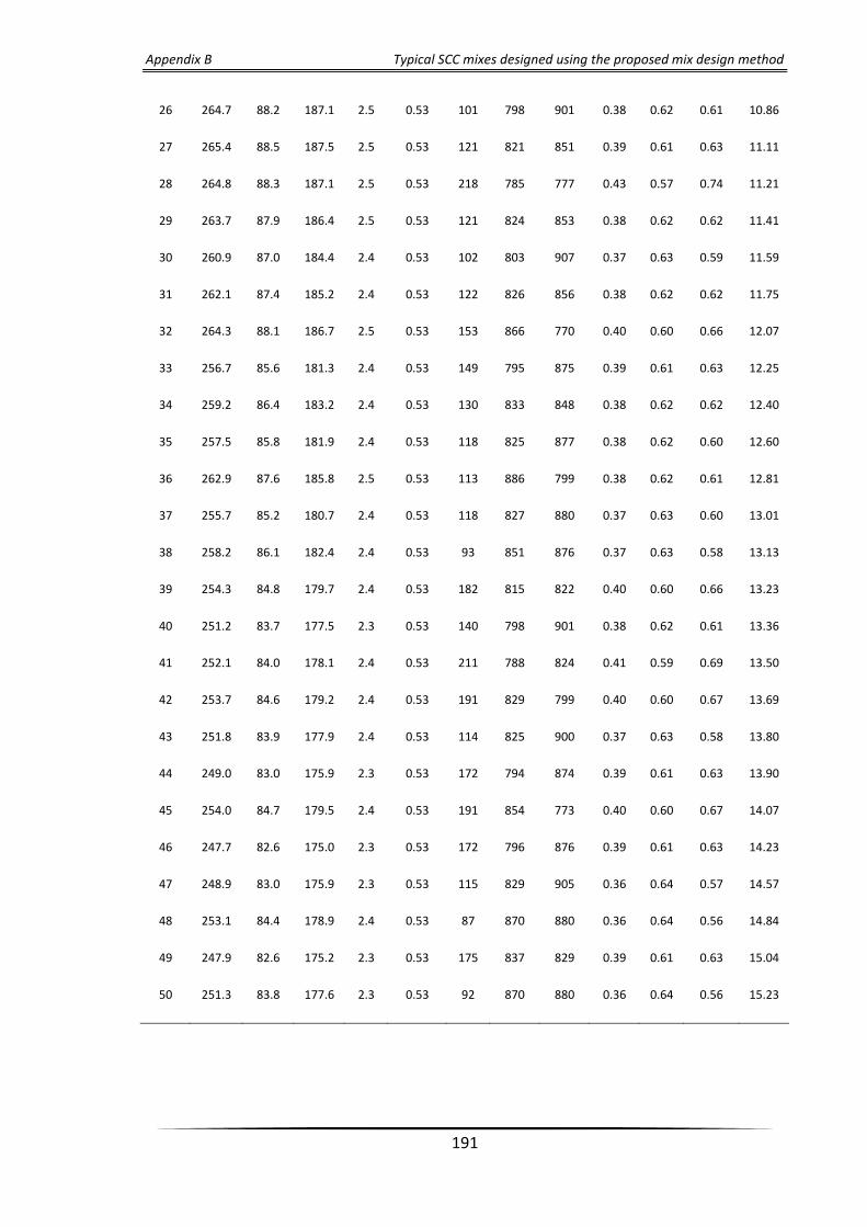
Appendix B Typical SCC mixes designed using the proposed mix design method
191
26 264.7 88.2 187.1 2.5 0.53 101 798 901 0.38 0.62 0.61 10.86
27 265.4 88.5 187.5 2.5 0.53 121 821 851 0.39 0.61 0.63 11.11
28 264.8 88.3 187.1 2.5 0.53 218 785 777 0.43 0.57 0.74 11.21
29 263.7 87.9 186.4 2.5 0.53 121 824 853 0.38 0.62 0.62 11.41
30 260.9 87.0 184.4 2.4 0.53 102 803 907 0.37 0.63 0.59 11.59
31 262.1 87.4 185.2 2.4 0.53 122 826 856 0.38 0.62 0.62 11.75
32 264.3 88.1 186.7 2.5 0.53 153 866 770 0.40 0.60 0.66 12.07
33 256.7 85.6 181.3 2.4 0.53 149 795 875 0.39 0.61 0.63 12.25
34 259.2 86.4 183.2 2.4 0.53 130 833 848 0.38 0.62 0.62 12.40
35 257.5 85.8 181.9 2.4 0.53 118 825 877 0.38 0.62 0.60 12.60
36 262.9 87.6 185.8 2.5 0.53 113 886 799 0.38 0.62 0.61 12.81
37 255.7 85.2 180.7 2.4 0.53 118 827 880 0.37 0.63 0.60 13.01
38 258.2 86.1 182.4 2.4 0.53 93 851 876 0.37 0.63 0.58 13.13
39 254.3 84.8 179.7 2.4 0.53 182 815 822 0.40 0.60 0.66 13.23
40 251.2 83.7 177.5 2.3 0.53 140 798 901 0.38 0.62 0.61 13.36
41 252.1 84.0 178.1 2.4 0.53 211 788 824 0.41 0.59 0.69 13.50
42 253.7 84.6 179.2 2.4 0.53 191 829 799 0.40 0.60 0.67 13.69
43 251.8 83.9 177.9 2.4 0.53 114 825 900 0.37 0.63 0.58 13.80
44 249.0 83.0 175.9 2.3 0.53 172 794 874 0.39 0.61 0.63 13.90
45 254.0 84.7 179.5 2.4 0.53 191 854 773 0.40 0.60 0.67 14.07
46 247.7 82.6 175.0 2.3 0.53 172 796 876 0.39 0.61 0.63 14.23
47 248.9 83.0 175.9 2.3 0.53 115 829 905 0.36 0.64 0.57 14.57
48 253.1 84.4 178.9 2.4 0.53 87 870 880 0.36 0.64 0.56 14.84
49 247.9 82.6 175.2 2.3 0.53 175 837 829 0.39 0.61 0.63 15.04
50 251.3 83.8 177.6 2.3 0.53 92 870 880 0.36 0.64 0.56 15.23

Appendix B Typical SCC mixes designed using the proposed mix design method
192
Table B.4: Mix constituents (kg/m3) for mixes grade 60
Mix No.
cm Water SP w/cm LP FA CA
Paste Vol.
Solid Vol.
p/s ratio
𝜂𝑚𝑖𝑥 Pa s Cem. ggbs
1 346.80 115.60 217.30 3.24 0.47 124 718 762 0.46 0.54 0.84 6.01
2 338.40 112.80 212.00 3.16 0.47 137 715 776 0.45 0.55 0.83 6.57
3 336.08 112.03 210.60 3.14 0.47 137 718 780 0.45 0.55 0.82 6.75
4 334.20 111.40 209.40 3.12 0.47 115 731 798 0.44 0.56 0.78 6.89
5 334.50 111.50 209.60 3.12 0.47 135 728 777 0.45 0.55 0.81 6.91
6 332.40 110.80 208.30 3.10 0.47 109 723 820 0.43 0.57 0.77 6.96
7 332.85 110.95 208.60 3.11 0.47 116 733 800 0.44 0.56 0.78 7.01
8 330.68 110.23 207.20 3.09 0.47 136 733 782 0.44 0.56 0.80 7.24
9 327.60 109.20 205.30 3.06 0.47 145 718 797 0.44 0.56 0.80 7.41
10 325.43 108.48 204.00 3.04 0.47 133 734 801 0.44 0.56 0.78 7.65
11 322.43 107.48 202.00 3.01 0.47 146 725 805 0.44 0.56 0.78 7.90
12 320.78 106.93 201.00 2.99 0.47 147 727 807 0.44 0.56 0.78 8.06
13 320.40 106.80 200.80 2.99 0.47 149 733 799 0.44 0.56 0.78 8.15
14 321.53 107.18 201.50 3.00 0.47 162 760 752 0.44 0.56 0.80 8.32
15 320.33 106.78 200.80 2.99 0.47 162 762 754 0.44 0.56 0.80 8.45
16 316.43 105.48 198.30 2.95 0.47 150 738 805 0.43 0.57 0.77 8.57
17 314.03 104.68 196.80 2.93 0.47 158 722 820 0.43 0.57 0.77 8.71
18 318.83 106.28 199.80 2.98 0.47 110 803 775 0.42 0.58 0.72 8.81
19 311.40 103.80 195.10 2.91 0.47 159 726 823 0.43 0.57 0.76 9.01
20 314.10 104.70 196.80 2.93 0.47 161 778 757 0.44 0.56 0.77 9.23
21 308.55 102.85 193.40 2.88 0.47 162 734 819 0.43 0.57 0.76 9.41
22 312.15 104.05 195.60 2.91 0.47 151 799 752 0.43 0.57 0.75 9.61
23 304.58 101.53 190.90 2.84 0.47 148 739 843 0.42 0.58 0.72 9.84
24 309.08 103.03 193.70 2.89 0.47 132 806 777 0.42 0.58 0.72 9.97

Appendix B Typical SCC mixes designed using the proposed mix design method
193
25 303.30 101.10 190.10 2.83 0.47 163 741 827 0.43 0.58 0.74 10.10
26 308.25 102.75 193.20 2.88 0.47 140 818 758 0.42 0.58 0.73 10.25
27 305.18 101.73 191.20 2.85 0.47 148 803 775 0.42 0.58 0.73 10.48
28 298.28 99.43 186.90 2.78 0.47 154 745 849 0.42 0.58 0.71 10.72
29 299.70 99.90 187.80 2.80 0.47 142 777 825 0.41 0.59 0.70 10.86
30 298.95 99.65 187.30 2.79 0.47 176 768 797 0.43 0.57 0.74 11.04
31 296.03 98.68 185.50 2.76 0.47 195 735 820 0.43 0.57 0.75 11.21
32 299.40 99.80 187.60 2.79 0.47 149 811 782 0.41 0.59 0.71 11.37
33 299.03 99.68 187.40 2.79 0.47 100 827 824 0.39 0.61 0.65 11.60
34 294.38 98.13 184.50 2.75 0.47 108 792 866 0.39 0.61 0.64 11.75
35 299.85 99.95 187.90 2.80 0.47 115 854 775 0.40 0.60 0.67 11.92
36 291.30 97.10 182.50 2.72 0.47 102 784 890 0.39 0.61 0.63 12.12
37 297.75 99.25 186.60 2.78 0.47 116 857 778 0.40 0.60 0.66 12.30
38 289.43 96.48 181.40 2.70 0.47 102 787 893 0.38 0.62 0.62 12.48
39 287.63 95.88 180.20 2.69 0.47 161 769 849 0.41 0.59 0.69 12.66
40 295.20 98.40 185.00 2.76 0.47 116 861 781 0.40 0.60 0.66 12.81
41 288.60 96.20 180.90 2.69 0.47 146 810 820 0.40 0.60 0.67 13.07
42 289.95 96.65 181.70 2.71 0.47 141 832 798 0.40 0.60 0.67 13.21
43 287.03 95.68 179.90 2.68 0.47 147 812 822 0.40 0.60 0.67 13.38
44 288.30 96.10 180.60 2.69 0.47 141 835 800 0.40 0.60 0.66 13.56
45 286.88 95.63 179.80 2.68 0.47 94 829 866 0.38 0.62 0.61 13.74
46 287.48 95.83 180.20 2.68 0.47 158 842 776 0.41 0.59 0.68 13.90
47 288.23 96.08 180.60 2.69 0.47 90 851 844 0.38 0.62 0.61 13.99
48 285.60 95.20 179.00 2.67 0.47 163 842 776 0.41 0.59 0.68 14.28
49 280.05 93.35 175.50 2.61 0.47 162 792 847 0.40 0.60 0.66 14.43
50 284.10 94.70 178.00 2.65 0.47 164 844 778 0.40 0.60 0.68 14.62

Appendix B Typical SCC mixes designed using the proposed mix design method
194
Table B.5: Mix constituents (kg/m3) for mixes grade 70
Mix No.
cm Water SP w/cm LP FA CA
Paste Vol.
Solid Vol.
p/s ratio
𝜂𝑚𝑖𝑥 Pa s Cem. ggbs
1 376.73 125.58 200.90 3.52 0.40 127 698 784 0.46 0.54 0.84 7.06
2 374.03 124.68 199.50 3.49 0.40 151 690 773 0.46 0.54 0.86 7.29
3 372.00 124.00 198.40 3.47 0.40 128 704 791 0.45 0.55 0.82 7.41
4 368.48 122.83 196.50 3.44 0.40 130 718 784 0.45 0.55 0.81 7.77
5 364.13 121.38 194.20 3.40 0.40 131 724 790 0.44 0.56 0.80 8.14
6 367.58 122.53 196.00 3.43 0.40 110 775 750 0.44 0.56 0.78 8.21
7 362.18 120.73 193.20 3.38 0.40 131 726 792 0.44 0.56 0.80 8.31
8 365.48 121.83 194.90 3.41 0.40 110 778 753 0.44 0.56 0.78 8.40
9 362.18 120.73 193.10 3.38 0.40 161 733 750 0.46 0.54 0.84 8.51
10 361.13 120.38 192.60 3.37 0.40 108 761 786 0.43 0.57 0.76 8.61
11 360.98 120.33 192.50 3.37 0.40 130 768 753 0.44 0.56 0.79 8.75
12 358.88 119.63 191.40 3.35 0.40 108 763 789 0.43 0.57 0.76 8.83
13 357.90 119.30 190.90 3.34 0.40 108 765 790 0.43 0.57 0.75 8.93
14 353.70 117.90 188.70 3.30 0.40 130 742 801 0.43 0.57 0.77 9.17
15 353.48 117.83 188.50 3.30 0.40 140 765 765 0.44 0.56 0.78 9.46
16 350.33 116.78 186.90 3.27 0.40 130 746 806 0.43 0.57 0.76 9.53
17 352.05 117.35 187.80 3.29 0.40 140 767 767 0.44 0.56 0.77 9.62
18 348.00 116.00 185.60 3.25 0.40 131 749 809 0.43 0.57 0.75 9.80
19 348.83 116.28 186.10 3.26 0.40 141 771 771 0.43 0.57 0.77 9.98
20 347.78 115.93 185.50 3.25 0.40 141 772 773 0.43 0.57 0.76 10.11
21 339.00 113.00 180.80 3.16 0.40 139 738 837 0.42 0.58 0.73 10.69
22 337.35 112.45 179.90 3.15 0.40 139 739 839 0.42 0.58 0.73 10.90
23 335.63 111.88 179.00 3.13 0.40 140 741 841 0.42 0.58 0.72 11.13
24 334.05 111.35 178.20 3.12 0.40 140 743 844 0.42 0.58 0.72 11.35

Appendix B Typical SCC mixes designed using the proposed mix design method
195
25 335.63 111.88 179.00 3.13 0.40 148 771 801 0.42 0.58 0.73 11.53
26 337.80 112.60 180.10 3.15 0.40 124 809 783 0.42 0.58 0.71 11.67
27 332.03 110.68 177.10 3.10 0.40 137 758 838 0.41 0.59 0.71 11.78
28 336.38 112.13 179.40 3.14 0.40 124 811 785 0.41 0.59 0.71 11.88
29 330.53 110.18 176.30 3.09 0.40 137 760 840 0.41 0.59 0.70 11.99
30 336.60 112.20 179.50 3.14 0.40 124 828 766 0.41 0.59 0.71 12.11
31 333.90 111.30 178.10 3.12 0.40 125 814 788 0.41 0.59 0.70 12.27
32 330.08 110.03 176.00 3.08 0.40 149 778 808 0.42 0.58 0.72 12.37
33 334.05 111.35 178.20 3.12 0.40 124 831 769 0.41 0.59 0.70 12.52
34 331.88 110.63 177.00 3.10 0.40 127 820 784 0.41 0.59 0.70 12.66
35 328.50 109.50 175.20 3.07 0.40 93 799 855 0.39 0.61 0.65 12.80
36 331.20 110.40 176.60 3.09 0.40 125 835 773 0.41 0.59 0.69 13.01
37 324.23 108.08 172.90 3.03 0.40 138 778 838 0.41 0.59 0.69 13.16
38 328.05 109.35 175.00 3.06 0.40 128 825 789 0.41 0.59 0.69 13.32
39 322.58 107.53 172.00 3.01 0.40 139 780 840 0.41 0.59 0.68 13.45
40 325.20 108.40 173.50 3.04 0.40 146 814 788 0.41 0.59 0.70 13.63
41 319.43 106.48 170.30 2.98 0.40 122 773 874 0.40 0.60 0.66 13.81
42 323.85 107.95 172.70 3.02 0.40 146 815 789 0.41 0.59 0.70 13.89
43 321.23 107.08 171.30 3.00 0.40 139 798 823 0.40 0.60 0.68 14.00
44 317.78 105.93 169.50 2.97 0.40 123 775 876 0.39 0.61 0.65 14.11
45 322.43 107.48 171.90 3.01 0.40 114 825 820 0.40 0.60 0.65 14.25
46 328.50 109.50 175.20 3.07 0.40 98 878 766 0.40 0.61 0.65 14.34
47 315.98 105.33 168.50 2.95 0.40 123 777 879 0.39 0.61 0.65 14.45
48 317.85 105.95 169.50 2.97 0.40 143 800 825 0.40 0.60 0.68 14.62
49 315.08 105.03 168.00 2.94 0.40 100 789 896 0.38 0.62 0.62 14.84
50 325.35 108.45 173.50 3.04 0.40 98 883 770 0.39 0.61 0.64 15.01

Appendix B Typical SCC mixes designed using the proposed mix design method
196
Table B.6: Mix constituents (kg/m3) for mixes grade 80
Mix No.
cm
Water SP w/cm LP FA CA Paste Vol.
Solid Vol.
p/s ratio
𝜂𝑚𝑖𝑥 Pa s
Cem. ggbs
1 396.83 132.28 185.20 3.70 0.35 116 689 824 0.45 0.55 0.80 8.01
2 398.63 132.88 186.00 3.72 0.35 116 720 786 0.45 0.55 0.81 8.10
3 400.13 133.38 186.70 3.74 0.35 114 749 755 0.45 0.55 0.81 8.20
4 394.43 131.48 184.10 3.68 0.35 117 725 791 0.44 0.56 0.80 8.45
5 389.48 129.83 181.70 3.63 0.35 114 692 842 0.44 0.56 0.78 8.57
6 391.65 130.55 182.80 3.66 0.35 104 734 804 0.44 0.56 0.77 8.69
7 386.55 128.85 180.40 3.61 0.35 115 696 846 0.44 0.56 0.77 8.82
8 384.83 128.28 179.60 3.59 0.35 112 693 857 0.43 0.57 0.76 8.93
9 387.68 129.23 180.90 3.62 0.35 105 739 809 0.43 0.57 0.76 9.06
10 382.43 127.48 178.50 3.57 0.35 112 696 860 0.43 0.57 0.76 9.15
11 388.95 129.65 181.50 3.63 0.35 113 767 767 0.44 0.56 0.78 9.23
12 378.90 126.30 176.80 3.54 0.35 115 687 875 0.43 0.57 0.75 9.39
13 386.25 128.75 180.30 3.61 0.35 114 770 770 0.43 0.57 0.77 9.49
14 376.65 125.55 175.80 3.52 0.35 116 689 878 0.43 0.57 0.74 9.61
15 383.03 127.68 178.70 3.58 0.35 107 771 785 0.43 0.57 0.75 9.78
16 374.55 124.85 174.80 3.50 0.35 114 697 876 0.42 0.58 0.74 9.87
17 373.35 124.45 174.20 3.48 0.35 115 699 878 0.42 0.58 0.73 10.00
18 377.63 125.88 176.20 3.53 0.35 101 757 822 0.42 0.58 0.73 10.13
19 378.08 126.03 176.40 3.53 0.35 108 776 791 0.42 0.58 0.74 10.32
20 374.78 124.93 174.90 3.51 0.35 101 760 825 0.42 0.58 0.72 10.45
21 373.28 124.43 174.20 3.45 0.35 105 760 825 0.42 0.58 0.72 10.61
22 376.35 125.45 175.60 3.48 0.35 114 797 766 0.43 0.57 0.74 10.76
23 369.38 123.13 172.40 3.49 0.35 103 742 857 0.41 0.59 0.71 10.81
24 374.40 124.80 174.70 3.43 0.35 115 799 769 0.42 0.58 0.74 11.00
25 367.20 122.40 171.40 3.42 0.35 98 752 857 0.41 0.59 0.69 11.16

Appendix B Typical SCC mixes designed using the proposed mix design method
197
26 366.23 122.08 170.90 3.40 0.35 111 758 838 0.41 0.59 0.71 11.37
27 364.65 121.55 170.20 3.43 0.35 98 755 861 0.41 0.59 0.69 11.49
28 368.03 122.68 171.70 3.38 0.35 113 802 786 0.42 0.58 0.71 11.75
29 361.73 120.58 168.80 3.40 0.35 99 759 864 0.41 0.60 0.68 11.89
30 364.20 121.40 170.00 3.33 0.35 97 796 821 0.41 0.59 0.69 12.11
31 357.30 119.10 166.70 3.39 0.35 95 747 892 0.40 0.60 0.66 12.27
32 363.23 121.08 169.50 3.32 0.35 102 806 806 0.41 0.59 0.69 12.40
33 355.28 118.43 165.80 3.37 0.35 95 749 895 0.40 0.60 0.66 12.57
34 361.20 120.40 168.50 3.34 0.35 103 809 808 0.41 0.59 0.68 12.71
35 357.53 119.18 166.80 3.29 0.35 104 788 838 0.40 0.60 0.68 12.87
36 352.35 117.45 164.40 3.32 0.35 96 753 899 0.39 0.61 0.65 13.02
37 355.58 118.53 165.90 3.35 0.35 104 790 841 0.40 0.60 0.67 13.18
38 359.18 119.73 167.60 3.33 0.35 109 830 784 0.41 0.59 0.69 13.34
39 357.30 119.10 166.70 3.23 0.35 104 823 802 0.40 0.60 0.68 13.49
40 345.98 115.33 161.50 3.27 0.35 101 734 930 0.39 0.61 0.64 13.64
41 350.48 116.83 163.60 3.21 0.35 108 783 858 0.40 0.60 0.66 13.79
42 344.18 114.73 160.60 3.30 0.35 102 736 932 0.39 0.61 0.64 13.94
43 353.63 117.88 165.00 3.27 0.35 105 827 806 0.40 0.60 0.67 14.13
44 350.48 116.83 163.60 3.32 0.35 98 810 840 0.39 0.61 0.65 14.29
45 355.80 118.60 166.00 3.18 0.35 100 862 769 0.40 0.60 0.67 14.48
46 340.95 113.65 159.10 3.25 0.35 97 747 934 0.38 0.62 0.62 14.64
47 347.70 115.90 162.30 3.31 0.35 99 813 844 0.39 0.61 0.64 14.81
48 354.30 118.10 165.30 3.21 0.35 95 872 769 0.40 0.60 0.66 14.96
49 343.80 114.60 160.50 3.18 0.35 93 797 878 0.39 0.61 0.63 15.13
50 340.88 113.63 159.10 3.11 0.35 91 777 910 0.38 0.62 0.62 15.24

Appendix C
Passing-ability test results of wide bar spacing
(10 bars) J-ring apparatus

Appendix C Passing-ability test results of wide bar spacing J-ring apparatus
199
Table C.1: t500J and difference between flow and J-ring spread diameter
Mix designation t500j, s D flow, mm D J-ring, mm D flow – D J-ring, mm
30A 0.60 685 665 20
40A 0.74 730 710 20
50A(50A) 1.40(1.31) 675(670) 660(650) 15(20)
60A 1.48 665 640 25
70A 1.79 700 700 0
80A 2.43 730 705 25
Figure C.1: Flow and passing ability of SCC mix: 30A (Left), 50A (Right)
Figure C.2: Flow and passing ability of SCC mix: 70A (Left), 80A (Right)

Appendix C Passing-ability test results of wide bar spacing J-ring apparatus
200
Figure C.3: Flow and passing ability of SCC mix (50A)
Figure C.4: t500J time versus plastic viscosity
y = 0.0394x2 - 0.2752x + 0.9946R² = 0.9653
0.0
0.5
1.0
1.5
2.0
2.5
3.0
4.0 5.0 6.0 7.0 8.0 9.0 10.0 11.0
t 50
0J,
s
Plastic viscosity, Pa s

Appendix C Passing-ability test results of wide bar spacing J-ring apparatus
201
Figure C.5: Plastic viscosity versus t500 and t500J
y = 0.028x2 - 0.1766x + 0.6953R² = 0.9633
y = 0.0394x2 - 0.2752x + 0.9946R² = 0.9653
0.0
0.5
1.0
1.5
2.0
2.5
3.0
4.0 5.0 6.0 7.0 8.0 9.0 10.0 11.0
Tim
e, s
Plastic viscosity, Pa s
t500
t500J-ring

Appendix D
Experimental load-deflection diagrams for
deep and shallow notched specimens of SCC
subjected to TPB test
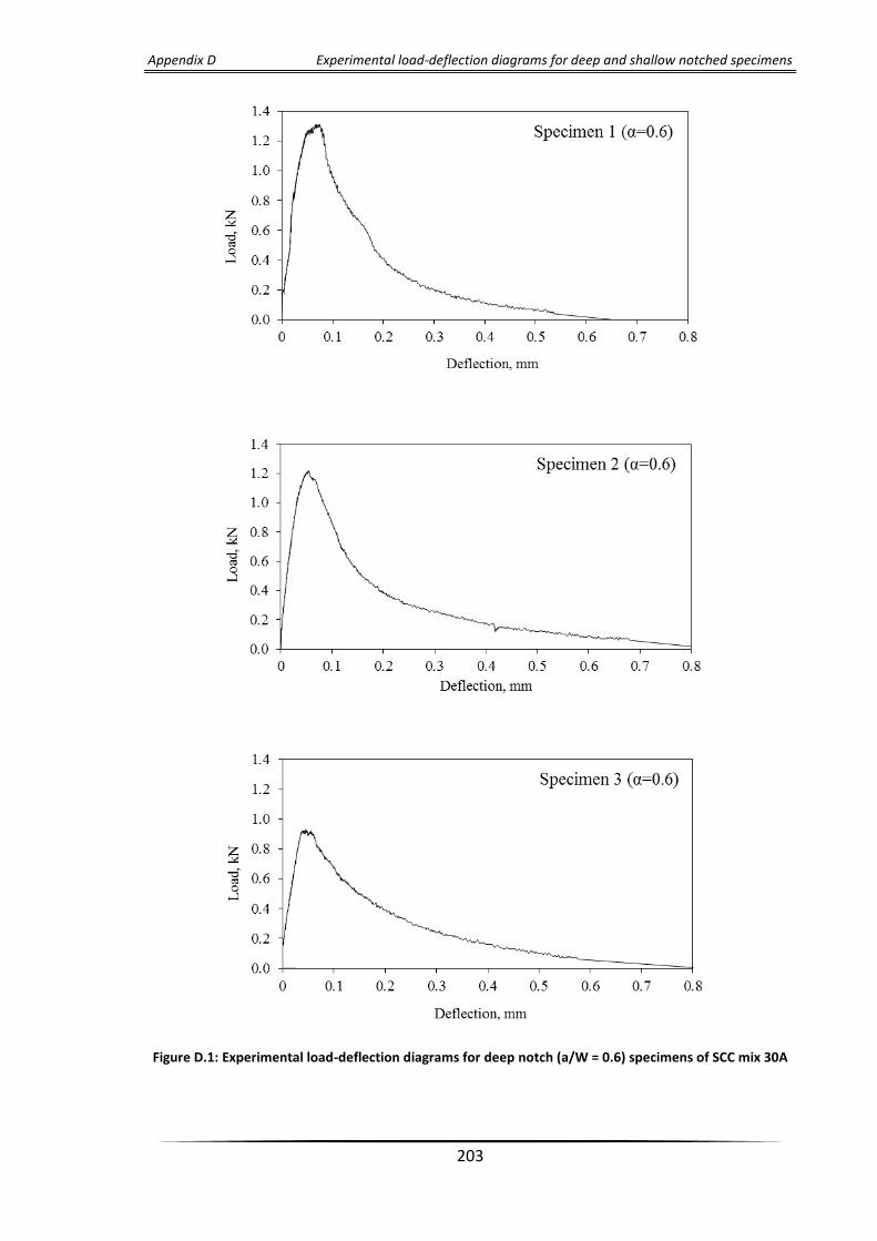
Appendix D Experimental load-deflection diagrams for deep and shallow notched specimens
203
Figure D.1: Experimental load-deflection diagrams for deep notch (a/W = 0.6) specimens of SCC mix 30A

Appendix D Experimental load-deflection diagrams for deep and shallow notched specimens
204
Figure D.2: Experimental load-deflection diagrams for shallow notch (a/W = 0.1) specimens of SCC mix
30A
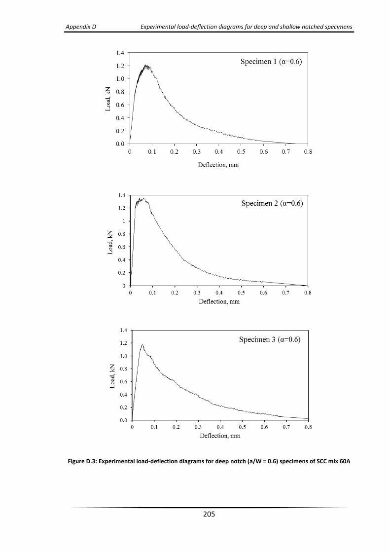
Appendix D Experimental load-deflection diagrams for deep and shallow notched specimens
205
Figure D.3: Experimental load-deflection diagrams for deep notch (a/W = 0.6) specimens of SCC mix 60A

Appendix D Experimental load-deflection diagrams for deep and shallow notched specimens
206
Figure D.4: Experimental load-deflection diagrams for shallow notch (a/W = 0.1) specimens of SCC mix
60A

Appendix D Experimental load-deflection diagrams for deep and shallow notched specimens
207
Figure D.5: Experimental load-deflection diagrams for deep notch (a/W = 0.6) specimens of SCC mix 80A
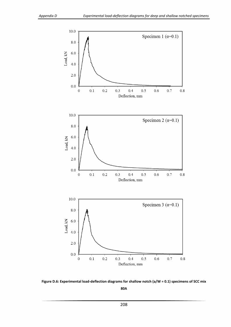
Appendix D Experimental load-deflection diagrams for deep and shallow notched specimens
208
Figure D.6: Experimental load-deflection diagrams for shallow notch (a/W = 0.1) specimens of SCC mix
80A

Appendix E
Experimental load-CMOD diagrams for deep
and shallow notched specimens of SCC
subjected to TPB test

Appendix E Experimental load-CMOD diagrams for deep and shallow notched specimens
210
Figure E.1: Experimental load-CMOD diagrams for deep notch (a/W = 0.6) specimens of SCC mix 30A

Appendix E Experimental load-CMOD diagrams for deep and shallow notched specimens
211
Figure E.2: Experimental load-CMOD diagrams for shallow notch (a/W = 0.1) specimens of SCC mix 30A

Appendix E Experimental load-CMOD diagrams for deep and shallow notched specimens
212
Figure E.3: Experimental load-CMOD diagrams for deep notch (a/W = 0.6) specimens of SCC mix 60A

Appendix E Experimental load-CMOD diagrams for deep and shallow notched specimens
213
Figure E.4: Experimental load-CMOD diagrams for shallow notch (a/W = 0.1) specimens of SCC mix 60A

Appendix E Experimental load-CMOD diagrams for deep and shallow notched specimens
214
Figure E.5: Experimental load-CMOD diagrams for deep notch (a/W = 0.6) specimens of SCC mix 80A

Appendix E Experimental load-CMOD diagrams for deep and shallow notched specimens
215
Figure E. 6: Experimental load-CMOD diagrams for shallow notch (a/W = 0.1) specimens of SCC mix 80A

Appendix F
A MATLAB program for determination of the
parameters of the bilinear tension softening
diagram (TSD)

Appendix F A MATLAB program for determination of the parameters of the bilinear TSD
217
%*******************************************************************
% CARDIFF UNIVERSITY
% SCHOOL OF ENGINEERING
% A MATLAB code for Determination of the static response of self-
% compacting concrete beams under three-point bending, using a
% bilinear tension-softening (stress-crack opening) relationship
% based on the fictitious crack model.
%*******************************************************************
% References
% 1. Hillerborg A. (1980). Analysis of fracture by means of the
% fictitious crack model, particularly for fibre-reinforced
% concrete, Int J Cement Composites, 2, 177-184.
% 2. Hillerborg A., Modeer M. and Petersson P. (1976). Analysis of
% crack formation and crack growth in concrete by means of
% fracture mechanics and finite elements, Cement Concrete
% Research, 6, 773-782.
% 3. Olesen J.F. (2001). Fictitious crack propagation in fibre-
% reinforced concrete beams, J Engineering Mechanics, 127, 272-80
%*******************************************************************
% List of variables
% Name Description
% ----- ------------
% alp0 Initial notch depth to beam depth ratio
% db beam depth, mm
% h Height of the hinge, mm
% L Span length of the TPB, mm
% t Thickness of the hinge, mm
% S Width of the hinge, mm
% al, a2, b1 & b2 Parameters for the bilinear relation
% a1 & a2 1/mm
% b1 & b2 Dimensionless
% E Young modulus, GPa
% ft Splitting tensile strength, GPa
% GF Specific size-independent fracture energy
%*******************************************************************
%*******************************************************************
% Part one for calculation the shallow notch parameters
%*******************************************************************
%*******************************************************************

Appendix F A MATLAB program for determination of the parameters of the bilinear TSD
218
clc
clear all
close all
polyfitOrder = 30;
% Enter the path of the experimental results Excel files of load-
% CMOD curves
v_matpath='C: \Users\Wajde1975\Desktop\ Fracture\80B';
% Enter the maximum displacement of the shallow and deep notches
MaxDisplacement01=0.42;
MaxDisplacement06=0.30;
% Enter the beam dimensions details
L=400;
t=100;
db=100;
a0shallow=10;
a0deep=60;
% Enter the rho value (use 0 for plain concrete or 0.045 for fibre
reinforced concrete)
rho=0;
% Enter the selected sheets numbers for shallow samples
SheetNo1 = [1 2 3 4 5];
% Enter the selected sheets numbers for deep samples
SheetNo6 = [7 8 9 10 11];
% Enter a proposed values of minimum and maximum theta
themin=0;
themax=200;
increment=themax/499;
incrementxq=MaxDisplacement01/499;
% xq is a constant increments in the x-direction of the average
experimental load-CMOD curves
xq = 0: incrementxq:MaxDisplacement01;
% Change the path to the file location
cd(v_matpath)
% Find the excel files in the folder
files = dir ('*.xlsx');
% [status, sheets] = xlsfinfo (filename)
filename = files(1).name;
[AA BB] = size(SheetNo1);
for n=1:BB
% Read Microsoft Excel spreadsheet file
clear subsetA

Appendix F A MATLAB program for determination of the parameters of the bilinear TSD
219
sheet = SheetNo1(1,n);
% Enter column range of the Excel sheets
xlRange = 'A:E';
subsetA = xlsread(filename,sheet,xlRange);
%*******************************************************************
% Fit curve or surface to data
%*******************************************************************
% Enter the column number of the x value (CMOD column in the excel sheet)
x = subsetA (:, 5);
% Enter the column number of the y value (load column in the excel sheet)
y = subsetA (:, 3);
hold on
plot(x,y);
p = polyfit(x,y, polyfitOrder);
f = polyval(p,x);
ff = polyval(p,xq);
% save all the results in one matrix (each column is a excel file)
Final_results(:,n)= ff(1,:);
hold on
end
% find the average of the final matrix
[m z] = size(Final_results);
for i = 1:m
C(i,1) = mean(Final_results(i,1:z));
end
plot(xq,C,':.');
hold on
plot(x,y,'o');
%*******************************************************************
%Except parameters that can be used later on
%*******************************************************************
clearvars -except xq C polyfitOrder a0shallow a0deep db L t rho SheetNo6
v_matpath MaxDisplacement06 themin increment themax
%*******************************************************************
a0=a0shallow;
alp0=a0/db;
h=(1-alp0)*db;
s=0.5*h;
%*******************************************************************
% Enter a1, a2, b2, ft, E limits values
%*******************************************************************

Appendix F A MATLAB program for determination of the parameters of the bilinear TSD
220
count = 1;
for a1=1:0.5:50
for a2=0.1:0.05:1.5
for b2=0.1:0.05:0.9
for ft=0.0018:0.0001:0.0048
for E=25:0.5:40
bet1=ft*a1*s/E;
bet2=ft*a2*s/E;
c =(1-b2)*(1-bet1)/(bet2-bet1);
rho=0;
the01=1-rho ;
the12=.5*(1-rho-c+((1-rho-c)^2+c^2/(bet1-1))^0.5);
the23=.5*(rho*(bet2-1)+b2/bet2+(rho^2*(bet2-1)^2+2*rho*(bet2-
1)*b2/bet2+(1-b2)^2/(bet1 -bet2)+b2^2/bet2)^.5);
k=0;
for the=themin :increment: themax
%*******************************************************************
% Alpha & Mu Calculation
%*******************************************************************
% For phase 0
if (0<=the & the<=the01)
alp = 0;
mu = the;
cod = 0;
% For phase I
elseif(the01<the & the<=the12)
bi= 1;
beti = bet1;
alp = 1-bet1-((1-bet1)*((1-rho)/the-bet1))^.5;
mu = 4*(1-3*alp+3*alp^2-alp^3/(1-bet1))*the+(6*alp-3)*(1-rho);
cod = s*ft/E*(1-bi+2*alp*the)/(1-beti);
% For phase II
elseif(the12<the & the<=the23)
bi = b2;
beti = bet2;
alp =1-bet2-(1-b2)/(2*the)-(( 1-bet2)*(( 1-b2)^2/(4*the^2)/(bet1 -bet2)-
bet2+(b2-rho)/the))^.5;
mu = 4*(1-3*alp+3*alp^2-alp^3/(1-bet2))*the+(6*alp-3)*(1-rho)-(((1-
b2)*(3*alp^2-(c/(2*the))^2))/(1-bet2));
cod = s*ft/E*(1-bi+2*alp*the)/(1-beti);
% For phase III

Appendix F A MATLAB program for determination of the parameters of the bilinear TSD
221
elseif(the23<the)
bi =0;
beti = 0;
alp = 1 -1 /(2*the)*(1+((1-b2)^2/(bet1-bet2)+b2^2/bet2-4*rho*the)^.5);
mu = 4*(1-3*alp+3*alp^2-alp^3)*the+(6*alp-3)*(1-rho)-
3*alp^2+1/(4*the^2)*(1-b2/bet2)*(1-b2/bet2+c)*(1+bet1*c/(1-
bet1))+(c/(2*the))^2;
cod = s*ft/E*(1-bi+2*alp*the)/(1-beti);
end
k=k+1;
pp(k) = 2/3*ft*h^2*t/L*mu;
m = pp(k)*L/4;
sigm = 6*m/(t*db^2);
cod0 = 4*sigm*a0/E*(0.76-2.28*alp0+3.87*alp0^2-2.04*alp0^3+0.66/(1-
alp0)^2);
CMOD(k) = cod + cod0;
end
AA = [CMOD;pp]';
x = AA(:,1); % the x value
y = AA(:,2); % the y value
% select either spline fit or polyfit (choose one option as shown here)
%*******************************************************************
% spline fit option
ff=interp1(x,y,xq,'spline');
%*******************************************************************
% poly fit option
% p = polyfit(x,y, polyfitOrder);
% f = polyval(p,x);
% ff = polyval(p,xq);
%*******************************************************************
%Check the maximum differences in theoretical and experimental %peak
%load
%*******************************************************************H1=ma
x(ff);
H2=max(C);
H3=(H2-H1)/H2*100;
if(-2<=H3 && H3<=2)

Appendix F A MATLAB program for determination of the parameters of the bilinear TSD
222
clear Error
[mm nn]= size(xq);
for ii = 1:nn
Error(ii,2) = (ff(1,ii)-C(ii,1))^2;
Error(ii,1) = xq(1,ii);
end
SumError (count,1) = sum (Error(:,2))/nn;
SumError (count,2) = a1;
SumError (count,3) = a2;
SumError (count,4) = b2;
SumError (count,5) = ft;
SumError (count,6) = E;
count = count +1;
end
end
end
end
end
end
EE=sortrows(SumError,[1 6]);
MinERR=EE(1,1);
a1=EE(1,2);
a2=EE(1,3);
b2=EE(1,4);
ft=EE(1,5);
E=EE(1,6);
w1=(1-b2)/(a1-a2);
w2=b2/a2;
sigmaft=a2*(w2-w1);
Gf01=0.5*ft*1000*(w1+sigmaft*w2);
D=[0 w1 w2];
EEE=[1 sigmaft 0];
KneeCoordinatesSHallow= [D; EEE]';
%*******************************************************************
%Except parameters that can be used later on
%*******************************************************************
clearvars -except sigmaft C xq alp0 E ft db h L t s rho a1 a2 b2 themin
increment themax KneeCoordinatesSHallow w1 w2 Gf01 MinERR SumError
polyfitOrder a0 a0deep SheetNo6 v_matpath MaxDisplacement06 B1
%*******************************************************************
bet1=ft*a1*s/E;

Appendix F A MATLAB program for determination of the parameters of the bilinear TSD
223
bet2=ft*a2*s/E;
c =(1-b2)*(1-bet1)/(bet2-bet1);
rho=0;
the01=1-rho ;
the12=0.5*(1-rho-c+((1-rho-c)^2+c^2/(bet1-1))^0.5);
the23=0.5*(rho*(bet2-1)+b2/bet2+(rho^2*(bet2-1)^2+2*rho*(bet2-
1)*b2/bet2+(1-b2)^2/(bet1 -bet2)+b2^2/bet2)^.5);
k=0;
%*******************************************************************
%*******************************************************************
% Alpha & MU Calculation
%*******************************************************************
%*******************************************************************
% input theta values
for the=themin :increment:themax
% For phase 0
if (0<=the & the<=the01)
alp = 0;
mu = the;
cod = 0;
% For phase I
elseif(the01<the & the<=the12)
bi= 1;
beti = bet1;
alp = 1-bet1-((1-bet1)*((1-rho)/the-bet1))^.5;
mu = 4*(1-3*alp+3*alp^2-alp^3/(1-bet1))*the+(6*alp-3)*(1-rho);
cod = s*ft/E*(1-bi+2*alp*the)/(1-beti);
% For phase II
elseif(the12<the & the<=the23)
bi = b2;
beti = bet2;
alp =1-bet2-(1-b2)/(2*the)-(( 1-bet2)*(( 1-b2)^2/(4*the^2)/(bet1 -bet2)-
bet2+(b2-rho)/the))^.5;
mu = 4*(1-3*alp+3*alp^2-alp^3/(1-bet2))*the+(6*alp-3)*(1-rho)-(((1-
b2)*(3*alp^2-(c/(2*the))^2))/(1-bet2));
cod = s*ft/E*(1-bi+2*alp*the)/(1-beti);
% For phase III
elseif(the23<the)
bi =0;
beti = 0;
alp = 1 -1 /(2*the)*(1+((1-b2)^2/(bet1-bet2)+b2^2/bet2-4*rho*the)^.5);

Appendix F A MATLAB program for determination of the parameters of the bilinear TSD
224
mu = 4*(1-3*alp+3*alp^2-alp^3)*the+(6*alp-3)*(1-rho)-
3*alp^2+1/(4*the^2)*(1-b2/bet2)*(1-b2/bet2+c)*(1+bet1*c/(1-
bet1))+(c/(2*the))^2;
cod = s*ft/E*(1-bi+2*alp*the)/(1-beti);
end
k=k+1;
pp(k) = 2/3*ft*h^2*t/L*mu;
m = pp(k)*L/4;
sigm = 6*m/(t*db^2);
cod0 = 4*sigm*a0/E*(0.76-2.28*alp0+3.87*alp0^2-2.04*alp0^3+0.66/(1-
alp0)^2);
CMOD(k) = cod + cod0;
end
AA = [CMOD;pp]';
x = AA(:,1); % the x value
y = AA(:,2); % the y value
% select either spline fit or polyfit (choose one option as shown here)
%*******************************************************************
% spline fit option
ff=interp1(x,y,xq,'spline');
%*******************************************************************
% poly fit option
% p = polyfit(x,y,polyfitOrder);
% f = polyval(p,x);
% ff = polyval(p,xq);
%*******************************************************************
W1(:,1)=xq;
W2(:,1)=C;
W3(:,1)=ff;
ModelCurve = [xq;ff]';
TestCurve=[W1,W2];
ModelTestCurveShallow = [W1';W2';W3']';
HeaderNames1='xq,PTest,PModel';
% Preferable output sheet name printed here
fileName1 = 'ModelTest01.csv';
outid = fopen(fileName1, 'w+');
fprintf(outid, '%s', HeaderNames1);
fclose(outid);
dlmwrite(fileName1,ModelTestCurveShallow,'roffset',1,'-append',
'precision', 4);
disp(strcat('Generated report ''',fileName1,''''))

Appendix F A MATLAB program for determination of the parameters of the bilinear TSD
225
% Preferable output sheet name printed here
filename = 'Parameters.xlsx';
% Desired parameters to be printed in the output sheet
A =
{'a1','a2','b2','w1','w2','Gf01','ft01','E','MinERR';a1,a2,b2,w1,w2,Gf01,
ft,E,MinERR};
B1=[a1,a2,b2,Gf01,ft,E,MinERR];
sheet = 1;
xlRange = 'A';
xlswrite(filename,A,sheet,xlRange)
filename = 'Parameters.xlsx';
A = {'Xknee','Yknee';0,1;w1,sigmaft;w2,0};
sheet = 1;
xlRange = 'J';
xlswrite(filename,A,sheet,xlRange)
%*******************************************************************
%*******************************************************************
%*******************************************************************
% Part two for calculation the deep notch parameters
%*******************************************************************
clearvars -except polyfitOrder MaxDisplacement06 SheetNo6 a0deep db L t s
rho themin increment themax KneeCoordinatesSHallow v_matpath B1
%*******************************************************************
incrementxq = MaxDisplacement06/499;
xq = 0:incrementxq:MaxDisplacement06;
% change the path to the file location automatically
cd(v_matpath)
% find the excel files in the folder
files = dir('*.xlsx');
filename = files(1).name;
[AA BB] = size(SheetNo6);
for n=1:BB
% Read Microsoft Excel spreadsheet file
clear subsetA
sheet = SheetNo6(1,n);
xlRange = 'A:E';
subsetA = xlsread(filename,sheet,xlRange);
%*******************************************************************
% Fit curve or surface to data

Appendix F A MATLAB program for determination of the parameters of the bilinear TSD
226
%*******************************************************************
% Enter the column number of the x value (CMOD column in the excel
% sheet)
x = subsetA(:,5);
% Enter the column number of the y value (load column in the excel
% sheet)
y = subsetA(:,3);
hold on
plot(x,y);
p = polyfit(x,y,polyfitOrder);
f = polyval(p,x);
ff = polyval(p,xq);
% save all the results in one matrix (each column is a excel file)
Final_results(:,n)= ff(1,:);
hold on
end
% find the average of the final matrix
[m z] = size(Final_results);
for i = 1:m
C(i,1) = mean(Final_results(i,1:z));
end
plot(xq,C,':.');
clearvars -except xq C polyfitOrder L t s rho db themin increment themax
KneeCoordinatesSHallow a0deep B1
%*******************************************************************
% Enter constant values
%*******************************************************************
a0=a0deep;
alp0=a0/db;
h=(1-alp0)*db;
% Enter a1, a2, b2, ft, E limits values
count = 1;
for a1=1:0.5:50
for a2=0.1:0.05:1.5
for b2=0.1:0.05:0.9
for ft=0.0018:0.0001:0.0048
for E=25:0.5:40
bet1=ft*a1*s/E;
bet2=ft*a2*s/E;
c =(1-b2)*(1-bet1)/(bet2-bet1);
rho=0;

Appendix F A MATLAB program for determination of the parameters of the bilinear TSD
227
the01=1-rho ;
the12=.5*(1-rho-c+((1-rho-c)^2+c^2/(bet1-1))^0.5);
the23=.5*(rho*(bet2-1)+b2/bet2+(rho^2*(bet2-1)^2+2*rho*(bet2-
1)*b2/bet2+(1-b2)^2/(bet1 -bet2)+b2^2/bet2)^.5);
k=0;
for the=themin :increment:themax
%*******************************************************************
% Alpha & Mu Calculation
%*******************************************************************
% For phase 0
if (0<=the & the<=the01)
alp = 0;
mu = the;
cod = 0;
% For phase I
elseif(the01<the & the<=the12)
bi= 1;
beti = bet1;
alp = 1-bet1-((1-bet1)*((1-rho)/the-bet1))^.5;
mu = 4*(1-3*alp+3*alp^2-alp^3/(1-bet1))*the+(6*alp-3)*(1-rho);
cod = s*ft/E*(1-bi+2*alp*the)/(1-beti);
% For phase II
elseif(the12<the & the<=the23)
bi = b2;
beti = bet2;
alp =1-bet2-(1-b2)/(2*the)-(( 1-bet2)*(( 1-b2)^2/(4*the^2)/(bet1 -bet2)-
bet2+(b2-rho)/the))^.5;
mu = 4*(1-3*alp+3*alp^2-alp^3/(1-bet2))*the+(6*alp-3)*(1-rho)-(((1-
b2)*(3*alp^2-(c/(2*the))^2))/(1-bet2));
cod = s*ft/E*(1-bi+2*alp*the)/(1-beti);
% For phase III
elseif(the23<the)
bi =0;
beti = 0;
alp = 1 -1 /(2*the)*(1+((1-b2)^2/(bet1-bet2)+b2^2/bet2-4*rho*the)^.5);
mu = 4*(1-3*alp+3*alp^2-alp^3)*the+(6*alp-3)*(1-rho)-
3*alp^2+1/(4*the^2)*(1-b2/bet2)*(1-b2/bet2+c)*(1+bet1*c/(1-
bet1))+(c/(2*the))^2;
cod = s*ft/E*(1-bi+2*alp*the)/(1-beti);

Appendix F A MATLAB program for determination of the parameters of the bilinear TSD
228
end
k=k+1;
pp(k) = 2/3*ft*h^2*t/L*mu;
m = pp(k)*L/4;
sigm = 6*m/(t*db^2);
cod0 = 4*sigm*a0/E*(0.76-2.28*alp0+3.87*alp0^2-2.04*alp0^3+0.66/(1-
alp0)^2);
CMOD(k) = cod + cod0;
end
AA = [CMOD;pp]';
x = AA(:,1); % the x value
y = AA(:,2); % the y value
% select either spline fit or polyfit (choose one option as shown)
%*******************************************************************
% spline fit option
ff=interp1(x,y,xq,'spline');
%*******************************************************************
% poly fit option
% p = polyfit(x,y,polyfitOrder);
% f = polyval(p,x);
% ff = polyval(p,xq);
%*******************************************************************
%Check the maximum differences in theoretical and experimental peak %load
%*******************************************************************H1=ma
x(ff);
H2=max(C);
H3=(H2-H1)/H2*100;
if(-2<=H3 && H3<=2)
clear Error
[mm nn]= size(xq);
for ii = 1:nn
Error(ii,2) = (ff(1,ii)-C(ii,1))^2;
Error(ii,1) = xq(1,ii);
end
SumError(count,1) = sum (Error(:,2))/nn;
SumError(count,2) = a1;
SumError(count,3) = a2;
SumError(count,4) = b2;
SumError(count,5) = ft;
SumError(count,6) = E;
count = count +1;

Appendix F A MATLAB program for determination of the parameters of the bilinear TSD
229
end
end
end
end
end
end
EE=sortrows(SumError,[1 6]);
MinERR=EE(1,1);
a1=EE(1,2);
a2=EE(1,3);
b2=EE(1,4);
ft=EE(1,5);
E=EE(1,6);
w1=(1-b2)/(a1-a2);
w2=b2/a2;
sigmaft=a2*(w2-w1);
Gf06=0.5*ft*1000*(w1+sigmaft*w2);
D=[0 w1 w2];
EEE=[1 sigmaft 0];
KneeCoordinatesSHallow=[D;EEE]';
%*******************************************************************
clearvars -except sigmaft C xq alp0 E ft db h L t s rho a1 a2 b2 themin
increment themax KneeCoordinatesDeep w1 w2 Gf01 Gf06 MinERR SumError
polyfitOrder a0deep KneeCoordinatesSHallow B1
%*******************************************************************
% input a1, a2, b2 values
a0=a0deep;
bet1=ft*a1*s/E;
bet2=ft*a2*s/E;
c =(1-b2)*(1-bet1)/(bet2-bet1);
rho=0;
the01=1-rho ;
the12=.5*(1-rho-c+((1-rho-c)^2+c^2/(bet1-1))^0.5);
the23=.5*(rho*(bet2-1)+b2/bet2+(rho^2*(bet2-1)^2+2*rho*(bet2-
1)*b2/bet2+(1-b2)^2/(bet1 -bet2)+b2^2/bet2)^.5);
k=0;
% input theta values
for the=themin :increment:themax
%*******************************************************************
% Alpha & Mu Calculation
%*******************************************************************

Appendix F A MATLAB program for determination of the parameters of the bilinear TSD
230
% For phase 0
if (0<=the & the<=the01)
alp = 0;
mu = the;
cod = 0;
% For phase I
elseif(the01<the & the<=the12)
bi= 1;
beti = bet1;
alp = 1-bet1-((1-bet1)*((1-rho)/the-bet1))^.5;
mu = 4*(1-3*alp+3*alp^2-alp^3/(1-bet1))*the+(6*alp-3)*(1-rho);
cod = s*ft/E*(1-bi+2*alp*the)/(1-beti);
% For phase II
elseif(the12<the & the<=the23)
bi = b2;
beti = bet2;
alp =1-bet2-(1-b2)/(2*the)-(( 1-bet2)*(( 1-b2)^2/(4*the^2)/(bet1 -bet2)-
bet2+(b2-rho)/the))^.5;
mu = 4*(1-3*alp+3*alp^2-alp^3/(1-bet2))*the+(6*alp-3)*(1-rho)-(((1-
b2)*(3*alp^2-(c/(2*the))^2))/(1-bet2));
cod = s*ft/E*(1-bi+2*alp*the)/(1-beti);
% For phase III
elseif(the23<the)
bi =0;
beti = 0;
alp = 1 -1 /(2*the)*(1+((1-b2)^2/(bet1-bet2)+b2^2/bet2-4*rho*the)^.5);
mu = 4*(1-3*alp+3*alp^2-alp^3)*the+(6*alp-3)*(1-rho)-
3*alp^2+1/(4*the^2)*(1-b2/bet2)*(1-b2/bet2+c)*(1+bet1*c/(1-
bet1))+(c/(2*the))^2;
cod = s*ft/E*(1-bi+2*alp*the)/(1-beti);
end
k=k+1;
pp(k) = 2/3*ft*h^2*t/L*mu;
m = pp(k)*L/4;
sigm = 6*m/(t*db^2);
cod0 = 4*sigm*a0/E*(0.76-2.28*alp0+3.87*alp0^2-2.04*alp0^3+0.66/(1-
alp0)^2);
CMOD(k) = cod + cod0;
end
AA = [CMOD;pp]';
x = AA(:,1); % the x value

Appendix F A MATLAB program for determination of the parameters of the bilinear TSD
231
y = AA(:,2); % the y value
% select either spline fit or polyfit (choose one option as shown)
%*******************************************************************
% spline fit option
ff=interp1(x,y,xq,'spline');
%************************************************************************
**
% poly fit option
% p = polyfit(x,y,polyfitOrder);
% f = polyval(p,x);
% ff = polyval(p,xq);
%*******************************************************************
W1(:,1)=xq;
W2(:,1)=C;
W3(:,1)=ff;
ModelCurve = [xq;ff]';
TestCurve=[W1,W2];
ModelTestCurveDeep = [W1';W2';W3']';
HeaderNames1='xq,PTest,PModel';
% Preferable output sheet name printed here
fileName1 = 'ModelTest06.csv';
outid = fopen(fileName1, 'w+');
fprintf(outid, '%s', HeaderNames1);
fclose(outid);
dlmwrite(fileName1,ModelTestCurveDeep,'roffset',1,'-append', 'precision',
4); % increased precision to allow all digits to be saved
disp(strcat('Generated report ''',fileName1,''''))
% Preferable output sheet name printed here
filename = 'Parameters.xlsx';
% Desired parameters to be printed in the output sheet
A
='a1','a2','b2','w1','w2','Gf06','ft06','E','MinERR';a1,a2,b2,w1,w2,Gf06,
ft,E,MinERR};
sheet = 1;
xlRange = 'L';
xlswrite(filename,A,sheet,xlRange)
filename = 'Parameters.xlsx';
A = {'Xknee','Yknee';0,1;w1,sigmaft;w2,0};
B2=[a1,a2,b2,Gf01,ft,E,MinERR];
parametersstar=(B1+B2)/2;
sheet = 1;

Appendix F A MATLAB program for determination of the parameters of the bilinear TSD
232
xlRange = 'U';
xlswrite(filename,A,sheet,xlRange)
%*******************************************************************
%*******************************************************************
%*******************************************************************
% This part is to find the unique parameters of hinge model
%*******************************************************************
% Enter constant values
%*******************************************************************
% Input the specific size-independent fracture energy, GF and
% splitting tensile strength, ft values
%*******************************************************************
%GF=0.1469; % Experimental simplified boundary effect method, N/m
%ft=3.12;% Experimental of splitting tensile strength, MPa
%*******************************************************************
a1star=parametersstar (1);
a2star=parametersstar (2);
b2star=parametersstar (3);
Gfstar=parametersstar (4);
ftstar=parametersstar(5)*1000;
w1star=(1-b2star)/(a1star-a2star)
w2star=b2star/a2star
w1=w1star*GF*ftstar/(Gfstar*ft);
sigmaftstar=(w2star-w1star)*a2star;
sigmaftstar2=1-a1star*w1star;
sigmastar=ftstar*sigmaftstar;
secondside=GF*sigmastar*w2star/(a2star*Gfstar*ft);
w2one=(w1+(w1^2+4*secondside)^0.5)/2
w2two=(w1-(w1^2+4*secondside)^0.5)/2
if(w2one>0)
w2=w2one
end
if(w2two>0)
w2=w2two
end
a2=a2star
sigmaft=(w2-w1)*a2;
a1=(1-sigmaft)/w1;
% Desired parameters to be printed in the output sheet
myMatrix=[a1star;a2star;ftstar;Gfstar;w1star;w2star;sigmaftstar;a1;a2;ft;
GF;w1;w2;sigmaft]';

Appendix F A MATLAB program for determination of the parameters of the bilinear TSD
233
% Preferable output sheet name printed here
fileName = 'Uniqueparameters.csv';
dlmwrite(fileName,myMatrix,'roffset',1,'-append', 'precision', 8);
disp(strcat('Generated report ''',fileName,''''))
%*******************************************************************
%*******************************************************************
%*******************************************************************

Appendix G
Simulation results of SCC mixes in 10 and 16-
bar J-ring tests

Appendix G Simulation results of SCC mixes in 10 and 16-bar J-ring test
235
Figure G.1: Flow pattern of SCC Mix30 just after passing through the gaps in 16-bar J-ring test (at 0.2 s)
Figure G.2: Flow pattern of SCC Mix30 at t500J in 16-bar J-ring test (at 0.7 s)
Figure G.3: Flow pattern of SCC Mix30 after it has stopped in 16-bar J-ring test (at 9.0 s)

Appendix G Simulation results of SCC mixes in 10 and 16-bar J-ring test
236
Figure G.4: Flow pattern of SCC Mix40 just after passing through the gaps in 16-bar J-ring test (at 0.3 s)
Figure G.5: Flow pattern of SCC Mix40 at t500J in 16-bar J-ring test (at 0.8 s)
Figure G.6: Flow pattern of SCC Mix40 after it has stopped in 16-bar J-ring test (at 12.0 s)

Appendix G Simulation results of SCC mixes in 10 and 16-bar J-ring test
237
Figure G.7: Flow pattern of SCC Mix50 just after passing through the gaps in 16-bar J-ring test (at 0.4 s)
Figure G.8: Flow pattern of SCC Mix50 at t500J in 16-bar J-ring test (at 1.4 s)
Figure G.9: Flow pattern of SCC Mix50 after it has stopped in 16-bar J-ring test (at 10.0 s)
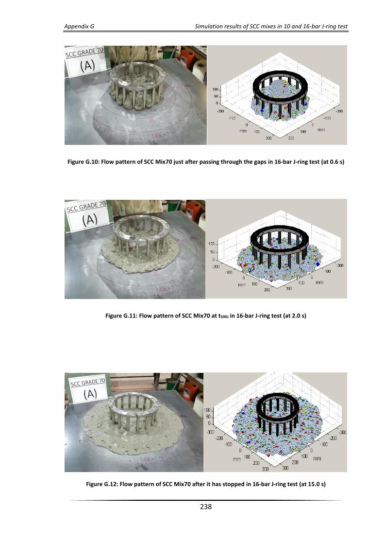
Appendix G Simulation results of SCC mixes in 10 and 16-bar J-ring test
238
Figure G.10: Flow pattern of SCC Mix70 just after passing through the gaps in 16-bar J-ring test (at 0.6 s)
Figure G.11: Flow pattern of SCC Mix70 at t500J in 16-bar J-ring test (at 2.0 s)
Figure G.12: Flow pattern of SCC Mix70 after it has stopped in 16-bar J-ring test (at 15.0 s)

Appendix G Simulation results of SCC mixes in 10 and 16-bar J-ring test
239
Figure G.13: Flow pattern of SCC Mix80 just after passing through the gaps in 16-bar J-ring test (at 0.8 s)
Figure G.14: Flow pattern of SCC Mix80 at t500J in 16-bar J-ring test (at 2.8 s)
Figure G.15: Flow pattern of SCC Mix80 after it has stopped in 16-bar J-ring test (at 16.0 s)

Appendix G Simulation results of SCC mixes in 10 and 16-bar J-ring test
240
Table G.1: Simulation and experimental results for SCC mixes of 10 bars J-ring
Mix
Designation
Plastic
viscosity, Pa
s
Yield
stress, Pa
t500J , s Spread diameter, mm
experimental simulated experimental simulated
30A 4.63 175 0.6 0.6 665 655
40A 6.84 175 0.7 0.7 710 690
50A 7.84 180 1.4 1.4 660 660
60A 8.18 175 1.5 1.4 640 645
70A 9.32 180 1.8 1.7 700 700
80A 10.47 190 2.4 2.3 705 710

Appendix G Simulation results of SCC mixes in 10 and 16-bar J-ring test
241
Figure G.16: Flow pattern of SCC Mix30 just after passing through the gaps in 10-bar J-ring test (at 0.2 s)
Figure G.17: Flow pattern of SCC Mix30 at t500J in 10-bar J-ring test (at 0.6 s)
Figure G.18: Flow pattern of SCC Mix30 after it has stopped in 10-bar J-ring test (at 10.0 s)

Appendix G Simulation results of SCC mixes in 10 and 16-bar J-ring test
242
Figure G.19: Flow pattern of SCC Mix40 just after passing through the gaps in 10-bar J-ring test (at 0.3 s)
Figure G.20: Flow pattern of SCC Mix40 at t500J in 10-bar J-ring test (at 0.7 s)
Figure G.21: Flow pattern of SCC Mix40 after it has stopped in 10-bar J-ring test (at 12.0 s)

Appendix G Simulation results of SCC mixes in 10 and 16-bar J-ring test
243
Figure G.22: Flow pattern of SCC Mix50 just after passing through the gaps in 10-bar J-ring test (at 0.4 s)
Figure G.23: Flow pattern of SCC Mix50 at t500J in 10-bar J-ring test (at 1.4 s)
Figure G.24: Flow pattern of SCC Mix50 after it has stopped in 10-bar J-ring test (at 11.0 s)

Appendix G Simulation results of SCC mixes in 10 and 16-bar J-ring test
244
Figure G.25: Flow pattern of SCC Mix60 just after passing through the gaps in 10-bar J-ring test (at 0.4 s)
Figure G.26: Flow pattern of SCC Mix60 at t500J in 10-bar J-ring test (at 1.5 s)
Figure G.27: Flow pattern of SCC Mix60 after it has stopped in 10-bar J-ring test (at 11.0 s)

Appendix G Simulation results of SCC mixes in 10 and 16-bar J-ring test
245
Figure G.28: Flow pattern of SCC Mix70 just after passing through the gaps in 10-bar J-ring test (at 0.6 s)
Figure G.29: Flow pattern of SCC Mix70 at t500J in 10-bar J-ring test (at 1.8 s)
Figure G.30: Flow pattern of SCC Mix70 after it has stopped in 10-bar J-ring test (at 16.0 s)

Appendix G Simulation results of SCC mixes in 10 and 16-bar J-ring test
246
Figure G.31: Flow pattern of SCC Mix80 just after passing through the gaps in 10-bar J-ring test (at 0.7 s)
Figure G.32: Flow pattern of SCC Mix80 at t500J in 10-bar J-ring test (at 2.4 s)
Figure G.33: Flow pattern of SCC Mix80 after it has stopped in 10-bar J-ring test (at 17.0 s)

Appendix G Simulation results of SCC mixes in 10 and 16-bar J-ring test
247
Figure G.34: The three concentric circular regions to evaluate the distribution of coarse aggregates in the
J-ring “pancake” of Mix70 in 10-bar J-ring test
Figure G.35: Coarse aggregate distributions in the three concentric circular regions in 10-bar J-ring test
0.0
0.2
0.4
0.6
0.8
1.0
(8-12) (12-16) (16-20) (>20)
CD
F
Coarse aggregate range size, mm
Region A Region B Region C

Appendix G Simulation results of SCC mixes in 10 and 16-bar J-ring test
248
Figure G.36: Four quadrants of Mix60 “pancake” to determine the aggregate distribution (10-bar J-ring
test)
Figure G.37: Coarse aggregate distributions in the four quadrants (10-bar J-ring test)
0.0
0.2
0.4
0.6
0.8
1.0
(8-12) (12-16) (16-20) (>20)
CD
F
Coarse aggregate range size, mm
Quadrant 1 Quadrant 2
Quadrant 3 Quadrant 4

Appendix G Simulation results of SCC mixes in 10 and 16-bar J-ring test
249
Figure G.38: Flow pattern of SCC (Mix40) showing the large aggregates in 10-bar J-ring test
Figure G.39: Coarse aggregate distributions along diametrical cross-sections (AA and BB) of Mix40
“pancake” in 10-bar J-ring test
AA
BB
AA
A
BB

Appendix G Simulation results of SCC mixes in 10 and 16-bar J-ring test
250
Figure G.40: Coarse aggregate distributions along the diametrical cross-sections (10-bar J-ring test)
0.0
0.2
0.4
0.6
0.8
1.0
(8-12) (12-16) (16-20) (>20)
CD
F
Coarse aggregate range size, mm
Section A-A Section B-B