design and simulation of an abs control scheme for a ... · the proposed scheme utilizes a cascade...
TRANSCRIPT

Design and Simulation of an ABS Control Schemefor a Formula Student Prototype
João Pedro Carrapiço Ferro
Thesis to obtain the Master of Science Degree in
Mechanical Engineering
Supervisor: Professor Paulo Jorge Coelho Ramalho
Co-supervisor: Professor João Miguel da Costa Sousa
Examination Committee
Chairperson:
Supervisor:
May 2014

2

Acknowledgments
The work developed in this thesis a continuance of the knowledge and innovative spirit acquired dur-
ing the three years spent in Projecto FST. For their unflagging help, suggestions and encouragement,
I would like to specially thank my team-mates, with whom I’ve designed, spent sleepless nights, dis-
cussed, learned, travelled, cheered, celebrated and shared the same passion for engineering and mo-
torsports.
To my thesis supervisor Professor Paulo Oliveira and co-supervisor Professor Joao Sousa, whose
insight, knowledge and advice were equally important on pursuing this ambitious but highly enlightening
challenge.
To my friends, for their motivation, everlasting friendship and comprehension when I just could not
be there.
To my family, for their inestimable support and incessant belief, not only during this work, but through-
out the entire degree. A special dedication to my grandfather, who provided me the inspiration and
engineering genes.
i

ii

Abstract
Anti-lock braking system (ABS) has the objective of controlling wheel slip so that maximum friction
force is attained while maintaining adequate steerability and stability during hard braking. Beyond the
inestimable contribution to road safety, ABS may also be used in racecars as a driving-aid system to
enhance braking performance.
This thesis addresses the design of an ABS seeking the implementation on a Formula Student racing
prototype. The proposed scheme utilizes a cascade control architecture: a PID-type fuzzy controller with
a Takagi-Sugeno-Kang fuzzy inference system is designed for wheel slip control on the outer loop, whilst
a brake pressure PD controller is adopted in the inner loop. Wheel slip estimation solution, resorted on
a complementary filter, is also developed.
The performance of the ABS is assessed with a full vehicle model, sustained by vehicle dynamic
principles. The model is integrated with brakeline dynamics and a tire friction model based on reliable
experimental data. Straight line brake simulations are performed and results are evaluated in terms of
braking efficiency and control robustness, under different and variable conditions. A complete lap within
a typical Formula Student circuit is also simulated, for the cases with and without ABS.
Keywords: anti-lock braking system (ABS), Formula Student, fuzzy controller, PID controller,
wheel slip estimation, vehicle model, tire model
iii

iv

Resumo
O sistema de travagem ABS (do ingles anti-lock braking system) tem o objetivo de controlar o escor-
regamento da roda de forma a atingir a maxima forca de atrito, mantendo dirigibilidade e estabilidade
suficientes durante uma travagem brusca. Para alem da inestimavel contribuicao para a seguranca
rodoviaria, o sistema ABS pode tambem ser usado em carros de competicao como sistema de as-
sistencia a conducao para melhorar o desempenho em travagem.
Esta tese trata do projeto de um sistema ABS para implementacao num prototipo de competicao
do tipo Formula Student. O esquema proposto utiliza uma arquitetura de controlo em cascata: um
controlador fuzzy do tipo PID com um sistema de inferencia fuzzy do genero Takagi-Sugeno-Kang e
projetado para o controlo do escorregamento da roda no anel exterior, enquanto para o anel interior e
adotado um controlador de pressao do tipo PD. Uma solucao de estimacao para o escorregamento da
roda, com recurso a uma solucao de filtro complementar, e tambem desenvolvida.
O desempenho do sistema ABS e avaliada com um modelo completo do veıculo, sustentado nos
princıpios da dinamica de veıculos. O modelo e integrado com a dinamica da linha de travagem e um
modelo de atrito do pneu baseado em dados experimentais fidedignos. Simulacoes de travagem em
linha reta sao executadas e os resultados examinados em termos de eficiencia de travagem e robustez
de controlo, sob condicoes diversas e variaveis. E tambem simulada uma volta completa a um circuito
de Formula Student tıpico, para os casos com e sem ABS.
Palavras-chave: sistema de travagem ABS, Formula Student, controlador fuzzy, controlador
PID, estimacao do escorregamento da roda, modelo de veıculo, modelo de pneu
v

vi
Contents
Acknowledgments . . . . . . . . . . . . . . . . . . . . . . . . . . . . . . . . . . . . . . . . . . . i
Abstract . . . . . . . . . . . . . . . . . . . . . . . . . . . . . . . . . . . . . . . . . . . . . . . . . iii
Resumo . . . . . . . . . . . . . . . . . . . . . . . . . . . . . . . . . . . . . . . . . . . . . . . . . v
List of Tables . . . . . . . . . . . . . . . . . . . . . . . . . . . . . . . . . . . . . . . . . . . . . . xi
List of Figures . . . . . . . . . . . . . . . . . . . . . . . . . . . . . . . . . . . . . . . . . . . . . xiv
List of Symbols . . . . . . . . . . . . . . . . . . . . . . . . . . . . . . . . . . . . . . . . . . . . . xvi
1 Introduction 1
1.1 Brief history of ABS . . . . . . . . . . . . . . . . . . . . . . . . . . . . . . . . . . . . . . . 1
1.2 Motivation (Formula Student) . . . . . . . . . . . . . . . . . . . . . . . . . . . . . . . . . . 2
1.3 Objective . . . . . . . . . . . . . . . . . . . . . . . . . . . . . . . . . . . . . . . . . . . . . 3
1.4 Work contributions . . . . . . . . . . . . . . . . . . . . . . . . . . . . . . . . . . . . . . . . 4
1.5 Outline . . . . . . . . . . . . . . . . . . . . . . . . . . . . . . . . . . . . . . . . . . . . . . . 5
2 Vehicle Dynamics 7
2.1 Global Overview . . . . . . . . . . . . . . . . . . . . . . . . . . . . . . . . . . . . . . . . . 7
2.2 Horizontal Dynamics . . . . . . . . . . . . . . . . . . . . . . . . . . . . . . . . . . . . . . . 8
2.3 Vertical Dynamics . . . . . . . . . . . . . . . . . . . . . . . . . . . . . . . . . . . . . . . . 11
2.3.1 Lagrange Method . . . . . . . . . . . . . . . . . . . . . . . . . . . . . . . . . . . . 11
2.3.2 Vehicle Loads . . . . . . . . . . . . . . . . . . . . . . . . . . . . . . . . . . . . . . . 15
2.3.3 Inverse Kinematics . . . . . . . . . . . . . . . . . . . . . . . . . . . . . . . . . . . . 18
2.3.4 Tire Vertical Load . . . . . . . . . . . . . . . . . . . . . . . . . . . . . . . . . . . . 19
2.4 Wheel Dynamics . . . . . . . . . . . . . . . . . . . . . . . . . . . . . . . . . . . . . . . . . 19
2.4.1 Free-body diagram . . . . . . . . . . . . . . . . . . . . . . . . . . . . . . . . . . . . 19
2.5 Brakeline Dynamics . . . . . . . . . . . . . . . . . . . . . . . . . . . . . . . . . . . . . . . 20
2.5.1 Steady-state equations . . . . . . . . . . . . . . . . . . . . . . . . . . . . . . . . . 21
2.5.2 Transient behaviour . . . . . . . . . . . . . . . . . . . . . . . . . . . . . . . . . . . 22
2.5.3 Hydraulic Modulator . . . . . . . . . . . . . . . . . . . . . . . . . . . . . . . . . . . 23
3 Tire Model 25
3.1 Types of models . . . . . . . . . . . . . . . . . . . . . . . . . . . . . . . . . . . . . . . . . 25
3.1.1 Pacejka Model . . . . . . . . . . . . . . . . . . . . . . . . . . . . . . . . . . . . . . 26
vii

3.1.2 Burkhardt Model . . . . . . . . . . . . . . . . . . . . . . . . . . . . . . . . . . . . . 28
3.1.3 Neural Network Model . . . . . . . . . . . . . . . . . . . . . . . . . . . . . . . . . . 28
3.2 Experimental Data . . . . . . . . . . . . . . . . . . . . . . . . . . . . . . . . . . . . . . . . 29
3.3 Data Fitting . . . . . . . . . . . . . . . . . . . . . . . . . . . . . . . . . . . . . . . . . . . . 31
3.3.1 Methodology for Pacejka and Burckhardt models . . . . . . . . . . . . . . . . . . . 31
3.3.2 Results . . . . . . . . . . . . . . . . . . . . . . . . . . . . . . . . . . . . . . . . . . 32
4 ABS Overview 35
4.1 Objectives of ABS . . . . . . . . . . . . . . . . . . . . . . . . . . . . . . . . . . . . . . . . 35
4.2 ABS Components . . . . . . . . . . . . . . . . . . . . . . . . . . . . . . . . . . . . . . . . 36
4.3 Wheel Slip Control . . . . . . . . . . . . . . . . . . . . . . . . . . . . . . . . . . . . . . . . 37
4.3.1 Longitudinal Slip Ratio . . . . . . . . . . . . . . . . . . . . . . . . . . . . . . . . . . 37
4.3.2 Control Problem Definition . . . . . . . . . . . . . . . . . . . . . . . . . . . . . . . . 38
4.3.3 Main difficulties . . . . . . . . . . . . . . . . . . . . . . . . . . . . . . . . . . . . . . 40
4.4 Control Methods . . . . . . . . . . . . . . . . . . . . . . . . . . . . . . . . . . . . . . . . . 41
4.4.1 Threshold Control . . . . . . . . . . . . . . . . . . . . . . . . . . . . . . . . . . . . 41
4.4.2 PID Control . . . . . . . . . . . . . . . . . . . . . . . . . . . . . . . . . . . . . . . . 41
4.4.3 Sliding-mode Control . . . . . . . . . . . . . . . . . . . . . . . . . . . . . . . . . . . 42
4.4.4 Intelligent Control . . . . . . . . . . . . . . . . . . . . . . . . . . . . . . . . . . . . . 43
5 Proposed Approach 45
5.1 Problem data and requirements . . . . . . . . . . . . . . . . . . . . . . . . . . . . . . . . . 45
5.1.1 FS Rules . . . . . . . . . . . . . . . . . . . . . . . . . . . . . . . . . . . . . . . . . 45
5.1.2 Competition characteristics . . . . . . . . . . . . . . . . . . . . . . . . . . . . . . . 46
5.1.3 FST 05e . . . . . . . . . . . . . . . . . . . . . . . . . . . . . . . . . . . . . . . . . . 46
5.2 Proposed Control Structure . . . . . . . . . . . . . . . . . . . . . . . . . . . . . . . . . . . 47
5.2.1 Inner Loop - Brake Pressure Controller . . . . . . . . . . . . . . . . . . . . . . . . 48
5.2.2 Outter Loop - Wheel Slip Controller . . . . . . . . . . . . . . . . . . . . . . . . . . . 49
5.3 Design Approach . . . . . . . . . . . . . . . . . . . . . . . . . . . . . . . . . . . . . . . . . 50
6 ABS Design 51
6.1 Brake Pressure Controller . . . . . . . . . . . . . . . . . . . . . . . . . . . . . . . . . . . . 51
6.1.1 PID Overview . . . . . . . . . . . . . . . . . . . . . . . . . . . . . . . . . . . . . . . 51
6.1.2 PWM Conversion . . . . . . . . . . . . . . . . . . . . . . . . . . . . . . . . . . . . . 52
6.1.3 Open/closed loop step response . . . . . . . . . . . . . . . . . . . . . . . . . . . . 53
6.1.4 PD Design . . . . . . . . . . . . . . . . . . . . . . . . . . . . . . . . . . . . . . . . 54
6.2 Wheel Slip Controller . . . . . . . . . . . . . . . . . . . . . . . . . . . . . . . . . . . . . . . 58
6.2.1 FIS Overview . . . . . . . . . . . . . . . . . . . . . . . . . . . . . . . . . . . . . . . 58
6.2.2 FIS Design . . . . . . . . . . . . . . . . . . . . . . . . . . . . . . . . . . . . . . . . 59
6.2.3 PID Gains Optimization . . . . . . . . . . . . . . . . . . . . . . . . . . . . . . . . . 62
viii

6.2.4 Reference Wheel Slip . . . . . . . . . . . . . . . . . . . . . . . . . . . . . . . . . . 62
6.3 Wheel Slip Estimator . . . . . . . . . . . . . . . . . . . . . . . . . . . . . . . . . . . . . . . 63
6.3.1 Complementary Filter . . . . . . . . . . . . . . . . . . . . . . . . . . . . . . . . . . 64
6.4 ABS Triggers . . . . . . . . . . . . . . . . . . . . . . . . . . . . . . . . . . . . . . . . . . . 65
6.4.1 Minimum brake pressure . . . . . . . . . . . . . . . . . . . . . . . . . . . . . . . . 65
6.4.2 Wheel slip and wheel slip rate trigger . . . . . . . . . . . . . . . . . . . . . . . . . 66
6.4.3 Low velocity trigger . . . . . . . . . . . . . . . . . . . . . . . . . . . . . . . . . . . . 66
7 Simulation Results and Analysis 67
7.1 Simulation Parameters . . . . . . . . . . . . . . . . . . . . . . . . . . . . . . . . . . . . . . 67
7.1.1 FST 05e Parameters . . . . . . . . . . . . . . . . . . . . . . . . . . . . . . . . . . . 67
7.2 Straight Line Hard Braking . . . . . . . . . . . . . . . . . . . . . . . . . . . . . . . . . . . . 67
7.2.1 Constant µ . . . . . . . . . . . . . . . . . . . . . . . . . . . . . . . . . . . . . . . . 69
7.2.2 Varying µ . . . . . . . . . . . . . . . . . . . . . . . . . . . . . . . . . . . . . . . . . 71
7.2.3 Without pressure controller . . . . . . . . . . . . . . . . . . . . . . . . . . . . . . . 72
7.3 Complete Lap . . . . . . . . . . . . . . . . . . . . . . . . . . . . . . . . . . . . . . . . . . . 72
8 Summary and Conclusions 77
8.1 Future work and research . . . . . . . . . . . . . . . . . . . . . . . . . . . . . . . . . . . . 79
Bibliography 83
A SAE Definitions 84
A.1 Axis Systems . . . . . . . . . . . . . . . . . . . . . . . . . . . . . . . . . . . . . . . . . . . 84
A.1.1 Earth-Fixed Axis System . . . . . . . . . . . . . . . . . . . . . . . . . . . . . . . . 84
A.1.2 Vehicle Axis System . . . . . . . . . . . . . . . . . . . . . . . . . . . . . . . . . . . 84
A.1.3 Intermediate Axis System . . . . . . . . . . . . . . . . . . . . . . . . . . . . . . . . 85
A.1.4 Tire Axis System . . . . . . . . . . . . . . . . . . . . . . . . . . . . . . . . . . . . . 85
A.2 Angles . . . . . . . . . . . . . . . . . . . . . . . . . . . . . . . . . . . . . . . . . . . . . . . 85
A.2.1 Vehicle Orientation . . . . . . . . . . . . . . . . . . . . . . . . . . . . . . . . . . . . 86
A.2.2 Tire Orientation . . . . . . . . . . . . . . . . . . . . . . . . . . . . . . . . . . . . . . 87
ix

x

List of Tables
2.1 Coordinates of tire i on the (X,Y ) axis system. . . . . . . . . . . . . . . . . . . . . . . . . 9
2.2 Hydraulic modulator solenoid valves. . . . . . . . . . . . . . . . . . . . . . . . . . . . . . . 23
3.1 Magic Formula coefficients . . . . . . . . . . . . . . . . . . . . . . . . . . . . . . . . . . . 26
3.2 MATLAB’s lsqcurvefit parameters [1]. . . . . . . . . . . . . . . . . . . . . . . . . . . . . 32
3.3 MSE fitting result for Pacejka, Burkhardt and Neural Network tire models. . . . . . . . . . 34
4.1 Closed-loop variables for wheel slip control. . . . . . . . . . . . . . . . . . . . . . . . . . . 40
5.1 Closed-loop variables for pressure control. . . . . . . . . . . . . . . . . . . . . . . . . . . . 48
6.1 Tuned PD gains for pressure controller. . . . . . . . . . . . . . . . . . . . . . . . . . . . . 57
6.2 Fuzzy sets and membership functions (MFs) parameters for inputs eSX and ∆eSX . . . . . 60
6.3 Takagi-Sugeno-Kang (TSK) consequent function parameters for output ∆prefb . . . . . . . 60
6.4 Fuzzy rules for wheel slip controller. . . . . . . . . . . . . . . . . . . . . . . . . . . . . . . 61
6.5 Tuned PID gains for fuzzy wheel slip controller. . . . . . . . . . . . . . . . . . . . . . . . . 62
7.1 FST 05e parameters. . . . . . . . . . . . . . . . . . . . . . . . . . . . . . . . . . . . . . . . 68
7.2 Other model and simulation parameters. . . . . . . . . . . . . . . . . . . . . . . . . . . . . 69
7.3 Braking distance and time results with and without ABS. . . . . . . . . . . . . . . . . . . . 70
7.4 Braking distance and time without PD pressure controller. . . . . . . . . . . . . . . . . . . 72
7.5 Lap time results with and without ABS for Autocross Event. . . . . . . . . . . . . . . . . . 74
8.1 Results summary with and without ABS. . . . . . . . . . . . . . . . . . . . . . . . . . . . . 79
xi

xii

List of Figures
1.1 ABS tests by Mercedes-Benz on S-Class passenger car, 1978. . . . . . . . . . . . . . . . 2
1.2 Team from Projecto FST and FST 05e prototype. . . . . . . . . . . . . . . . . . . . . . . . 3
2.1 Vehicle dynamics overview. . . . . . . . . . . . . . . . . . . . . . . . . . . . . . . . . . . . 8
2.2 Planar tire forces on vehicle’s corner i [2]. . . . . . . . . . . . . . . . . . . . . . . . . . . . 9
2.3 Planar vehicle dynamics [2]. . . . . . . . . . . . . . . . . . . . . . . . . . . . . . . . . . . . 10
2.4 7 DOFs vibrational model [2]. . . . . . . . . . . . . . . . . . . . . . . . . . . . . . . . . . . 11
2.5 Longitudinal load transfer. . . . . . . . . . . . . . . . . . . . . . . . . . . . . . . . . . . . . 16
2.6 Lateral load transfer. . . . . . . . . . . . . . . . . . . . . . . . . . . . . . . . . . . . . . . . 17
2.7 Aerodynamic load. . . . . . . . . . . . . . . . . . . . . . . . . . . . . . . . . . . . . . . . . 18
2.8 Freebody diagram of the wheel. . . . . . . . . . . . . . . . . . . . . . . . . . . . . . . . . . 20
2.9 Schematic of basic brakeline dynamics. . . . . . . . . . . . . . . . . . . . . . . . . . . . . 20
2.10 Step response of brakeline dynamics Tb(t) for τ = 0.1 s. . . . . . . . . . . . . . . . . . . . 22
2.11 Schematic of brakeline dynamics with hydraulic modulator. . . . . . . . . . . . . . . . . . 23
2.12 Schematic of a hydraulic modulator [3]. . . . . . . . . . . . . . . . . . . . . . . . . . . . . 23
2.13 Simulink implementation of the hydraulic modulator. . . . . . . . . . . . . . . . . . . . . . 24
3.1 Classification of tire models. . . . . . . . . . . . . . . . . . . . . . . . . . . . . . . . . . . . 25
3.2 Pacejka’s Magic Formula curve and geometric parameters. . . . . . . . . . . . . . . . . . 27
3.3 Artificial neural network (ANN) scheme. . . . . . . . . . . . . . . . . . . . . . . . . . . . . 28
3.4 Tire test at Tire Research Facility (TIRF) [4]. . . . . . . . . . . . . . . . . . . . . . . . . . 29
3.5 Data from a complete run. In red, data sample for FZT = {50, 150, 250, 350} lbs, α = γ =
0◦ and p = 69 kPa (10 psi). . . . . . . . . . . . . . . . . . . . . . . . . . . . . . . . . . . . 30
3.6 Plot of SX vs. FXT for four sweeps of different FZT . . . . . . . . . . . . . . . . . . . . . . 31
3.7 Pacejka Model vs. TTC Data for FZT = {150, 250, 350} lbs. . . . . . . . . . . . . . . . . . 33
3.8 Burkhardt Model vs TTC Data for different velocities. . . . . . . . . . . . . . . . . . . . . . 33
3.9 Neural Network Model vs. TTC Data for FZT = {150, 250, 350} lbs. . . . . . . . . . . . . . 34
4.1 Buildup of yaw moment induced by large differences in friction coefficients [5]. . . . . . . 36
4.2 Anti-lock braking system (ABS) components diagram. . . . . . . . . . . . . . . . . . . . . 36
4.3 ABS action zones. . . . . . . . . . . . . . . . . . . . . . . . . . . . . . . . . . . . . . . . . 39
xiii
4.4 ABS control loop components [5]: 1-Hydraulic Modulator, 2-Master Cylinder, 3-Wheel
caliper, 4-ECU. . . . . . . . . . . . . . . . . . . . . . . . . . . . . . . . . . . . . . . . . . . 39
4.5 ABS algorithm. . . . . . . . . . . . . . . . . . . . . . . . . . . . . . . . . . . . . . . . . . . 42
5.1 Formula Student Germany 2013 endurance event. . . . . . . . . . . . . . . . . . . . . . . 46
5.2 Proposed control structure. . . . . . . . . . . . . . . . . . . . . . . . . . . . . . . . . . . . 47
5.3 Schematic of brakeline dynamics and pressure controller. . . . . . . . . . . . . . . . . . . 48
5.4 Closed-loop schematic of wheel slip controller. . . . . . . . . . . . . . . . . . . . . . . . . 49
5.5 PID-type fuzzy controller scheme [6]. . . . . . . . . . . . . . . . . . . . . . . . . . . . . . . 49
6.1 PID controller scheme. . . . . . . . . . . . . . . . . . . . . . . . . . . . . . . . . . . . . . . 52
6.2 PWM conversion scheme [6]. . . . . . . . . . . . . . . . . . . . . . . . . . . . . . . . . . . 53
6.3 PWM implementation with fc = 50 Hz. . . . . . . . . . . . . . . . . . . . . . . . . . . . . . 53
6.4 Open-loop schematic for pressure control. . . . . . . . . . . . . . . . . . . . . . . . . . . . 54
6.5 Open-loop variable-step response. . . . . . . . . . . . . . . . . . . . . . . . . . . . . . . . 55
6.6 Closed-loop schematic for pressure control. . . . . . . . . . . . . . . . . . . . . . . . . . . 55
6.7 Closed-loop variable-step response. . . . . . . . . . . . . . . . . . . . . . . . . . . . . . . 56
6.8 Linearisable approximation of brakeline system (a = 400, b = 1.28, h = −0.22 and v = 100. 57
6.9 Step response of original and approximated system. . . . . . . . . . . . . . . . . . . . . . 57
6.10 Step response with PD controller for pcal. . . . . . . . . . . . . . . . . . . . . . . . . . . . 58
6.11 Fuzzy inference system diagram. . . . . . . . . . . . . . . . . . . . . . . . . . . . . . . . . 59
6.12 Membership functions of fuzzy inference system (FIS). . . . . . . . . . . . . . . . . . . . . 61
6.13 Output surfaces of FIS models for wheel slip controller. . . . . . . . . . . . . . . . . . . . . 62
6.14 Block diagram of vS estimation. . . . . . . . . . . . . . . . . . . . . . . . . . . . . . . . . . 63
6.15 Block diagram of complementary filter. . . . . . . . . . . . . . . . . . . . . . . . . . . . . . 64
6.16 Slip velocity vS estimation results with complementary filter. . . . . . . . . . . . . . . . . . 65
7.1 Comparative simulation results with (solid) and without (dashed) ABS. . . . . . . . . . . . 70
7.2 Simulation results with varying µ. . . . . . . . . . . . . . . . . . . . . . . . . . . . . . . . . 71
7.3 Control scheme without pressure inner loop. . . . . . . . . . . . . . . . . . . . . . . . . . . 72
7.4 Comparative simulation results with (solid) and without (dashed) pressure PID controller. 73
7.5 GG diagram of an Autocoross lap. . . . . . . . . . . . . . . . . . . . . . . . . . . . . . . . 74
7.6 Velocity plot over an Autocoross lap. . . . . . . . . . . . . . . . . . . . . . . . . . . . . . . 75
7.7 Brake plot over an Autocoross lap. . . . . . . . . . . . . . . . . . . . . . . . . . . . . . . . 76
A.1 Vehicle Axis System [7]. . . . . . . . . . . . . . . . . . . . . . . . . . . . . . . . . . . . . . 85
A.2 Tire and Wheel Axis System [7]. . . . . . . . . . . . . . . . . . . . . . . . . . . . . . . . . 86
A.3 Tire Force and Moment Nomenclature [7]. . . . . . . . . . . . . . . . . . . . . . . . . . . . 86
xiv
List of Symbols
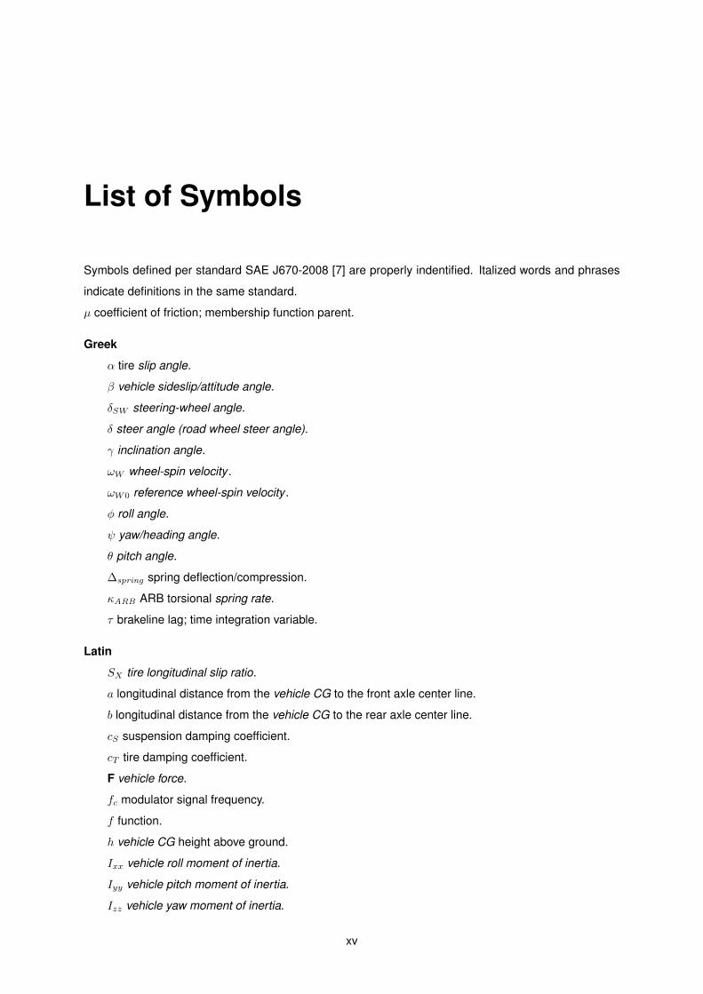
Symbols defined per standard SAE J670-2008 [7] are properly indentified. Italized words and phrases
indicate definitions in the same standard.
µ coefficient of friction; membership function parent.
Greek
α tire slip angle.
β vehicle sideslip/attitude angle.
δSW steering-wheel angle.
δ steer angle (road wheel steer angle).
γ inclination angle.
ωW wheel-spin velocity .
ωW0 reference wheel-spin velocity .
φ roll angle.
ψ yaw/heading angle.
θ pitch angle.
∆spring spring deflection/compression.
κARB ARB torsional spring rate.
τ brakeline lag; time integration variable.
Latin
SX tire longitudinal slip ratio.
a longitudinal distance from the vehicle CG to the front axle center line.
b longitudinal distance from the vehicle CG to the rear axle center line.
cS suspension damping coefficient.
cT tire damping coefficient.
F vehicle force.
fc modulator signal frequency.
f function.
h vehicle CG height above ground.
Ixx vehicle roll moment of inertia.
Iyy vehicle pitch moment of inertia.
Izz vehicle yaw moment of inertia.
xv

K gain.
kS suspension rate (wheel rate).
cdamper damping coefficient of suspension damper.
kspring spring rate of suspension spring.
kT tire normal stiffness (tire spring rate).
L wheelbase.
M vehicle moment .
m total vehicle total mass.
MR motion ratio.
ms sprung mass.
mu unsprung mass.
Re effective rolling radius.
RL tire loaded radius.
T track (track width, wheel track); time constant.
Ts sample time.
a vehicle acceleration.
v vehicle velocity .
xE , yE , zE earth-fixed coordinate system.
xV , yV , zV vehicle coordinate system.
X,Y, Z intermediate axis system.
z (w/ subscript) vertical displacement/travel (bounce/hop) in the direction of ZV .
Subscripts
bp brake pedal.
F front.
L left.
R rear; right.
r road/ground; DOF index.
s sprung mass.
T tire.
u unsprung mass/wheel.
X longitudinal/roll component.
Y lateral/pitch component.
Z vertical/yaw component.
xvi
Acronyms
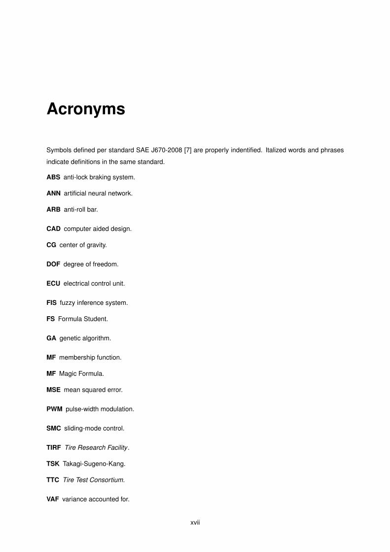
Symbols defined per standard SAE J670-2008 [7] are properly indentified. Italized words and phrases
indicate definitions in the same standard.
ABS anti-lock braking system.
ANN artificial neural network.
ARB anti-roll bar.
CAD computer aided design.
CG center of gravity.
DOF degree of freedom.
ECU electrical control unit.
FIS fuzzy inference system.
FS Formula Student.
GA genetic algorithm.
MF membership function.
MF Magic Formula.
MSE mean squared error.
PWM pulse-width modulation.
SMC sliding-mode control.
TIRF Tire Research Facility .
TSK Takagi-Sugeno-Kang.
TTC Tire Test Consortium.
VAF variance accounted for.
xvii

xviii

Chapter 1
Introduction
The ABS, also Antiblockier-Bremssystem in German, is an active safety system present in most of
passenger cars and trucks. Originally designed for aircrafts, it prevented the wheels from locking under
braking by regulating the brake line pressure independent of brake pedal force. Beyond simply avoiding
lock-up, modern ABSs manipulate wheel speed to achieve a desired slip level range where braking
distance is minimized while keeping steering stability.
Beyond the inestimable contribution to road safety, ABS may also be used in racecars as a driving-
aid device. By maximizing the braking force, the driver is able to brake later and while cornering, saving
precious time in every corner. Moreover, preventing the wheels from locking also considerably reduces
tire wear. Although forbidden in most high-end racing disciplines like Formula 1, driving-aids like ABS
are allowed in Formula Student (FS) and teams may benefit from its implementation.
1.1 Brief history of ABS
The first ABS dates back to 1929 and is credited to the french automobile and aircraft pioneer Gabriel
Voisin [8]. It was developed for aircraft use as threshold braking on airplanes is nearly impossible. Later
in 1945, the first set of mechanical ABS brakes were implemented on a Boeing B-47 to prevent spin outs
and tires from blowing [9]. In 1952, Dunlop’s Maxaret automatic and fully mechanical brake control was
one of the most important devices in the history of the aviation safety. Back then, considerably improved
braking efficiency and the elimination of the pilot’s fear of over-braking, which could result in skidding
and burst of tires, has resulted in a marked reduction in landing distances (up to 30%) [10]. ABS brakes
were commonly installed in airplanes thenceforth.
Though already acknowledged as a revolutionary system in the aviation scenery during the 1960s,
fully mechanical systems saw limited automobile use on high end automobiles only. In 1972, the british
Jensen lnterceptor automobile became the first production car to offer a Maxaret-based ABS. Low reli-
ability of system electronics and low public awareness, allied to the additional cost to the buyer, led to
their quiet withdrawal from the market in the middle 1970s [11].
1

The development of digital electronics changing from analog to integrated circuits and microproces-
sors resulted in a major automotive milestone with the introduction of the Bosch ABS systems on the
Mercedes-Benz S-Class passenger car in 1978 [11]. It was the first completely electronic four-wheel
multi-channel ABS system. BMW and others succeeded shortly. Japanese brake and vehicle manufac-
turers introduced ABS brakes based on the Bosch system as well as their own designs by the middle
1980s. The Bosch ABS system was used in 1986 Corvette and Cadillac Allante, followed by Ford in
1987. Since the late 1980s and early 1990s, ABS systems were found on nearly all top models of ev-
ery manufacturer. By the late 1990s, practically all passenger cars and light trucks were equipped with
four-wheel ABS systems, either as an option or standard equipment.
Figure 1.1: ABS tests by Mercedes-Benz on S-Class passenger car, 1978.
As more complete accident statistics became available over the years, the contribution of ABS to
road safety is now unquestionable and has already saved thousands of lives over the years. In the
European Union, all passenger cars require ABS as a standard equipment since 2007, as well as other
safety devices. This measure will be extended to motorcycles in 2016.
1.2 Motivation (Formula Student)
Formula Student is a motosport and engineering competition between university teams across the globe.
Students are challenged to design and build a single-seat racing car in order to compete in several events
worldwide. Teams are evaluated by experienced judges from professional motorsport and automotive
industry, not only according to the dynamic performance of the prototype but also regarding its design
and manufacturing features, cost analysis, and marketability.
At Instituto Superior Tecnico, the FS team was founded in 2001 under the name of Projecto FST
and has built its fifth and most innovative prototype in 2013: FST 05e. Featuring a complete carbon-fiber
monocoque, rims, suspension rods and aerodynamic package, two AC electric motors (55 kW in total)
are used to drive 230 kg from 0 to 100 km/h in less than 3 s.
2

Figure 1.2: Team from Projecto FST and FST 05e prototype.
Besides the great number of innovations presented in the FST 05e, an ABS system has never been
used by the team in any of their prototypes. Commercial ABS kits are very expensive and a self-made
design has been yet a very complex and time-consuming task. However, the constant seek for the best
performance possible allied with the experience attained by the the team and the availability of new
development tools (sensors on the car, computer car model) has cleared the path to the implementation
of this system for the first time.
1.3 Objective
The purpose of this work is thus to design and model an effective and reliable solution for the ABS control
problem that can also be simple and inexpensive to implement on a FS prototype. In other words, the
more favourable the following factors are, the better and more suitable the designed controller is:
Performance of the prototype in competition, measured in terms of lap times and/or overall score.
Implementation by Projecto FST team members on the upcoming prototypes, concerning required
knowledge, necessary components, assembling and maintenance.
Price of all components, excluding the ones already available on the prototype.
Although only computational design and simulation is performed here, it is also the intent of this
thesis to pave the way for further physical implementation of ABS on an upcoming prototype. It aims to
be both a learning tool and a design guide for actual and future team members of Projecto FST.
3
1.4 Work contributions
It is relevant to outline the following contributions present in this thesis:
• A self-developed vehicle model with 14 degrees of freedom (DOFs) was built for the design of the
ABS and subsequent simulation. The complete model, whose basis are described in Chapter 2,
includes the horizontal dynamics, relating tire longitudinal and lateral forces with the 3 DOFs for
vehicle position and orientation in the inertial reference plane; a 7-DOFs vibrational model of the
vehicle’s sprung and unsprung mass, integrated with load transfer and aerodynamic loads; a model
for the wheel dynamics, replicated for each corner, that outputs wheel angular velocity as a function
of the brake torque and tire longitudinal forces. Though the complete model is suitable for any four-
wheel vehicle, it is loaded with accurate parameters for the FST 05e prototype, measured either
experimentally or via CAD tools.
• Brakeline dynamics, relevant for ABS design, were modelled and integrated in the complete vehicle
model. It takes into account the hydraulic lag phenomenon and a pressure modulator model with
simple transient hydraulic equations.
• A tire model was designed and coupled with the full vehicle model using experimental tire data
outsourced from a renowned tire test facility. Three different fit models were used and compared,
including the well-known and widely used Pacejka’s Magic Formula (MF), the Burkhardt velocity-
dependant equation, and an self-developed new approach using artificial neural networks (ANNs).
• The proposed ABS control architecture resorts to a cascade structure with a brake pressure PD
controller in the inner loop and a self-developed PID-type fuzzy controller for wheel slip regulation
in the outer loop. Beyond clearly reducing the braking time and distance, results evidence the high
adaptability of a FIS to the nonlinear dynamics involved and robustness to model uncertainties and
external variances.
• A wheel slip estimator is designed using a complementary filter, i.e., a Wiener filter equivalent to
the stationary Kalman filter solution, which merges information provided by sensors (accelerometer
and wheel speed encoder) over distinct, yet complementary frequency regions. Moreover, this type
of filter ensures stability and a single design parameter representing a compromise responsiveness
and noise tolerance.
4
1.5 Outline
Chapter 2 presents the structure, concepts and mathematical basis that constitute the full vehicle model
and the integrated brakeline dynamics.
Chapter 3 describes the tire models tested in this work and the corresponding fitting to the experi-
mental tire data.
Chapter 4 introduces the main concepts and components of an ABS, and a problem definition from
the control theory point of view. The chapter ends with a literature review on the existing control methods.
Chapter 5 outlines the proposed control structure based on the available data and design require-
ments for the FST 05e prototype and the FS competition.
Chapter 6 describes the design of the ABS proposed in the previous chapter, including the pressure
controller, the wheel slip controller and the wheel slip estimator.
Chapter 7 presents the simulation results achieved with the ABS designed in Chapter 6. Different
and time-varying conditions are tested and the results are compared with the no-ABS situation.
Chapter 8 concludes this thesis by summarizing the main results and outlining further subjects to be
developed.
5

6

Chapter 2
Vehicle Dynamics
Vehicle dynamics is a very diverse and extensive topic. It refers to all the mechanical, physical or
aerodynamic principles governing the vehicle motion. For an ABS application, dynamics under braking
and tire-road interaction are the most important aspects to consider on a full vehicle model for further
controller design and simulation purposes. Hence, this chapter introduces the basic principles behind
the dynamics of the main sub-systems composing the aforementioned model.
After a global overview on the interdependencies between the subsystems (Section 2.1), the dy-
namics of each model are described in the following order: horizontal dynamics (Section 2.2); vertical
dynamics, including vibrational model, load transfer and aerodynamic (Section 2.3); wheel dynamics
(Section 2.4); brakeline dynamics with hydraulic modulator (Section 2.5).
2.1 Global Overview
The full vehicle model may be decomposed in five interconnected sub-models that are dependant on
each other, as depitected by the diagram in Fig. 2.1:
Horizontal dynamics is a 3-DOFs model for the kinematics of the vehicle’s center of gravity (CG) (ac-
celeration, velocity and position/heading) on an inertial reference plane, as a mass point subjected
to tire longitudinal and lateral forces from the Tire Model.
Vertical dynamics output the tire vertical load on each wheel, as a transient reaction force to the longi-
tudinal and lateral load transfers (due to acceleration) and the load due aerodynamics (dependent
on the velocity). Transient loads and displacements are measured by a 7-DOFs vibrational model
of the car’s suspension and tires.
Brakeline Dynamics model the hydraulic braking system, which for an ABS-equipped vehicle also in-
clude an hydraulic modulator. Given an external input of pedal brake force (also from the driver), it
outputs the brake torque that is sent to the Wheel Dynamics.
7
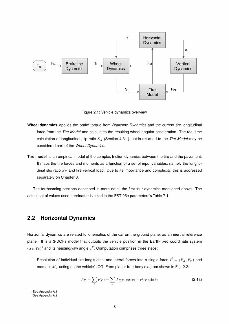
Figure 2.1: Vehicle dynamics overview.
Wheel dynamics applies the brake torque from Brakeline Dynamics and the current tire longitudinal
force from the Tire Model and calculates the resulting wheel angular acceleration. The real-time
calculation of longitudinal slip ratio SX (Section 4.3.1) that is returned to the Tire Model may be
considered part of the Wheel Dynamics.
Tire model is an empirical model of the complex friction dynamics between the tire and the pavement.
It maps the tire forces and moments as a function of a set of input variables, namely the longitu-
dinal slip ratio SX and tire vertical load. Due to its importance and complexity, this is addressed
separately on Chapter 3.
The forthcoming sections described in more detail the first four dynamics mentioned above. The
actual set of values used hereinafter is listed in the FST 05e parameters’s Table 7.1.
2.2 Horizontal Dynamics
Horizontal dynamics are related to kinematics of the car on the ground plane, as an inertial reference
plane. It is a 3-DOFs model that outputs the vehicle position in the Earth-fixed coordinate system
(XE ,YE)1 and its heading/yaw angle ψ2. Computation comprises three steps:
1. Resolution of individual tire longitudinal and lateral forces into a single force ~F = (FX , FY ) and
moment MZ acting on the vehicle’s CG. From planar free-body diagram shown in Fig. 2.2:
FX =∑i
FX,i =∑i
FXT,i cos δi − FY T,i sin δi (2.1a)
1See Appendix A.12See Appendix A.2
8

𝑌
𝐹𝑌𝑇,𝑖
𝐹𝑌,𝑖
𝑌𝑇
𝑋𝑇
𝐹𝑋𝑇,𝑖 𝐹𝑋,𝑖
𝑋 𝛿𝑖
𝑖
𝑀𝑍𝑇,𝑖
𝑍
Figure 2.2: Planar tire forces on vehicle’s corner i [2].
FY =∑i
FY,i =∑i
FY T,i sin δi + FY T,i cos δi (2.1b)
MZ =∑i
MZT,i −∑i
FX,i.yi +∑i
FY,i.xi (2.1c)
for i = FL, FR, RL, RR
where xi and yi designate the coordinates of tire i on the (X,Y ) axis system, as listed on Table 2.1.
i FL FR RL RR
xi a a −b −b
yiTF2 −TF2 TR
2 −TR2
Table 2.1: Coordinates of tire i on the (X,Y ) axis system.
2. Calculation of resulting forces FX and FY and moment MZ into linear and angular acceleration
and velocity of the vehicle axis system3. As explained in [2], Newton-Euler equations of planar
motion for a rigid body in a coordinate frame attached to CG are:
FX = m(aX − ψ vY
)(2.2a)
FY = m(aY + ψ vX
)(2.2b)
MZ = Izz ψ (2.2c)
where aX = vX and aY = vY represent the scalar value of the components of vehicle acceleration
3See Appendix A.1
9

𝑌𝐸
𝑋𝐸
𝑌
𝑋
𝐹𝑌
𝐹𝑋
𝑣𝑋
𝑣𝑌
𝒗
𝛽
𝜓
(𝑥𝐸 , 𝑦𝐸)
Figure 2.3: Planar vehicle dynamics [2].
vector ~a in the direction of the X and Y axis4, respectively.
3. Vehicle velocity and acceleration conversion from the vehicle axis system to the Earth-fixed axis
system. This is achieved through the use of a rotation matrix:
xE
yE
0
=
cosψ − sinψ 0
sinψ cosψ 0
0 0 1
vX
vY
0
(2.3)
4. Calculation of the vehicle’s path (position and yaw over time) by direct integration:
xE(t) = x0E +
∫ t
0
xE(τ) dτ (2.4a)
YE(t) = y0E +
∫ t
0
yE(τ) dτ (2.4b)
ψ(t) = ψ0 +
∫ t
0
ψ(τ) dτ (2.4c)
where x0E , y0
E and ψ0 refer to the the initial positions.
The vehicle sideslip angle5 is also computed in the Horizontal Dynamics model as follow:
β = arctanvYvX
(2.5)
4See Appendix A.15See Appendix A.2
10
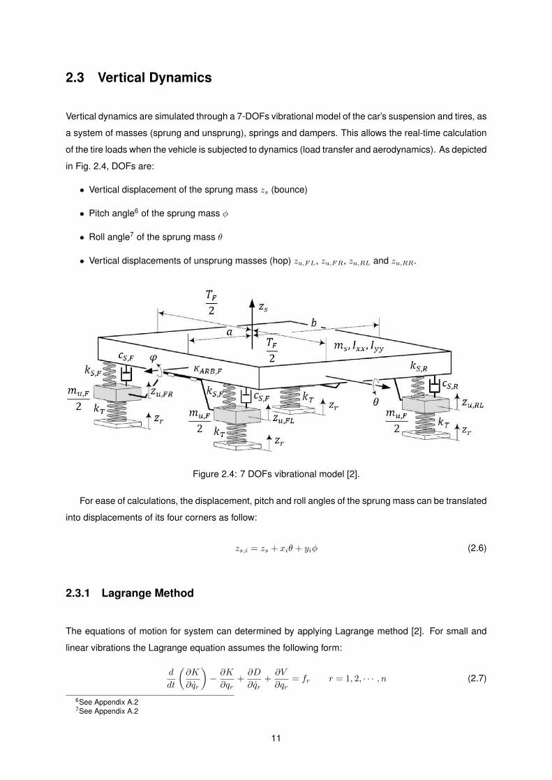
2.3 Vertical Dynamics
Vertical dynamics are simulated through a 7-DOFs vibrational model of the car’s suspension and tires, as
a system of masses (sprung and unsprung), springs and dampers. This allows the real-time calculation
of the tire loads when the vehicle is subjected to dynamics (load transfer and aerodynamics). As depicted
in Fig. 2.4, DOFs are:
• Vertical displacement of the sprung mass zs (bounce)
• Pitch angle6 of the sprung mass φ
• Roll angle7 of the sprung mass θ
• Vertical displacements of unsprung masses (hop) zu,FL, zu,FR, zu,RL and zu,RR.
Figure 2.4: 7 DOFs vibrational model [2].
For ease of calculations, the displacement, pitch and roll angles of the sprung mass can be translated
into displacements of its four corners as follow:
zs,i = zs + xiθ + yiφ (2.6)
2.3.1 Lagrange Method
The equations of motion for system can determined by applying Lagrange method [2]. For small and
linear vibrations the Lagrange equation assumes the following form:
d
dt
(∂K
∂qr
)− ∂K
∂qr+∂D
∂qr+∂V
∂qr= fr r = 1, 2, · · · , n (2.7)
6See Appendix A.27See Appendix A.2
11
where K, D and V are kinetic energy, dissipation function and potential energy, assuming the respective
forms
K =1
2mszs
2 +1
2Ixxφ
2 +1
2Iyy θ
2 +1
2
mu,F
2z2u,FL +
1
2
mu,F
2z2u,FR +
1
2
mu,R
2z2u,RL +
1
2
mu,R
2z2u,RR (2.8)
V =1
2kS,F
(zu,FL − zs + aθ +
TF2φ
)2
+1
2kS,F
(zu,FR − zs + aθ − TF
2φ
)2
+
1
2kS,R
(zu,RL − zs − bθ +
TR2φ
)2
+1
2kS,R
(zu,RR − zs − bθ −
TR2φ
)2
+
1
2kT (zr,FL − zu,FL)
2+
1
2kT (zr,FR − zu,FR)
2+
1
2kT (zr,RL − zu,RL)
2+
1
2kT (zr,RR − zu,RR)
2+
1
2κARB,F
(φ− zu,FL − zu,FR
TF
)2
+1
2κARB,R
(φ− zu,RL − zu,RR
TR
)2
(2.9)
D =1
2cS,F
(zu,FL − zs + aθ +
TF2φ
)2
+1
2cS,F
(zu,FR − zs + aθ − TF
2φ
)2
+
1
2cS,R
(zu,RL − zs − bθ +
TR2φ
)2
+1
2cS,R
(zu,RR − zs − bθ −
TR2φ
)2
+
1
2cT (zr,FL − zu,FL)
2+
1
2cT (zr,FR − zu,FR)
2+
1
2cT (zr,RL − zu,RL)
2+
1
2cT (zr,RR − zu,RR)
2 (2.10)
Since the suspension spring is not directly actuated, but through a series of suspension mechanisms
(tire to upright, pullrod/pushrod and bellcrank), an equivalent spring rate called suspension rate or wheel
rate, ks is used in the equations.
kS =kspringMR2
(2.11)
where MR stands for motion ratio, defined as
MR =zu − zs∆spring
(2.12)
The same rationale is applied to the damper, where cS is defined as
cS =cdamper
MR2(2.13)
Equation 2.7 is then evaluated for each one of the r = 1, . . . , 7 DOFs, from which a system of 7
independent differential equations is obtained. In the matrix form:
[M] {q}+ [C] {q}+ [K] {q} = {F} (2.14)
12

where [M], [C] and [K] are 7-by-7 matrices for the mass, damping and stiffness, respectively. The
vectors q, q and q represent the acceleration, velocity and position for each one of the 7 DOF’s.
[M] =
ms 0 0 0 0 0 0
0 Ixx 0 0 0 0 0
0 0 Iyy 0 0 0 0
0 0 0mu,F
2 0 0 0
0 0 0 0mu,F
2 0 0
0 0 0 0 0mu,R
2 0
0 0 0 0 0 0mu,R
2
(2.15)
[C] =
2 cS,F + 2 cS,R 0 #1 −cS,F −cS,F −cS,R −cS,R
0 #2 0 −cS,F TF2 cS,FTF2 −cS,R TR2 cS,R
TR2
#1 0 #3 a cS,F a cS,F −b cS,R −b cS,R
−cS,F −cS,F TF2 a cS,F cS,F + cT 0 0 0
−cS,F cS,FTF2 a cS,F 0 cS,F + cT 0 0
−cS,R −cS,R TR2 −b cS,R 0 0 cS,R + cT 0
−cS,R cS,RTR2 −b cS,R 0 0 0 cS,R + cT
(2.16)
#1 = 2 b cS,R − 2 a cS,F
#2 = cS,FTF
2
2+ cS,R
TR2
2
#3 = 2 cS,F a2 + 2 cS,R b
2
13

[K] =
2 kS,F + 2 kS,R 0 #1 −kS,F −kS,F −kS,R −kS,R
0 #2 0 −#4F #4F −#4R #4R
#1 0 #3 a kS,F a kS,F −b kS,R −b kS,R
−kS,F −#4F a kS,F #5F −κARB,F
TF 2 0 0
−kS,F #4F a kS,F −κARB,F
TF 2 #5F 0 0
−kS,R −#4R −b kS,R 0 0 #5R −κARB,R
TR2
−kS,R #4R −b kS,R 0 0 −κARB,R
TR2 #5R
(2.17)
#1 = 2 b kS,R − 2 a kS,F
#2 = kS,FTF
2
2+ kS,R
TR2
2+ κARB,F + κARB,R
#3 = 2 kS,F a2 + 2 kS,R b
2
#4i = kS,iTi2
+κARB,i
Ti
#5i = kS,i + kT +κARB,i
Ti2
The matrix of F is a 7-by-1 column matrix with the total forces on each DOF as a function of the
external forces Fs,i and Fu,i.
{F} =
−Fs,FL − Fs,FR − Fs,RL − Fs,RR
−Fs,FL TF2 + Fs,FRTF2 − Fs,RL TR2 + Fs,RR
TR2
Fs,FL a+ Fs,FR a− Fs,RL b− Fs,RR b−Mθ
cT zr,FL − Fu,FL + kT zr,FL
cT zr,FR − Fu,FR + kT zr,FR
cT zr,RL − Fu,RL + kT zr,RL
cT zr,RR − Fu,RR + kT zr,RR
(2.18)
14
2.3.2 Vehicle Loads
At any point in time, the vehicle’s sprung and unsprung masses are is subjected to the following types
of load:
• Static load
• Dynamic load
– Load Transfer
– Aerodynamics
Static Load
Static load corresponds to the load when the car is stationary and subjected to its own weight. Simple
free-body diagram calculations for the sprung and unsprung mass result in:
F sts,FL = F sts,FR =ms g
2
b
L(2.19a)
F sts,RL = F sts,RR =ms g
2
a
L(2.19b)
F stu,FL = F stu,FR =mu,F g
2(2.19c)
F stu,RL = F stu,RR =mu,R g
2(2.19d)
Weight Transfer Load
When the car accelerates, inertial forces are generated on the CG of the sprung and unsprung masses.
For a positive longitudinal accelerations (drive), this has the effect of transferring the load from the front
to the rear axle, whilst a positive lateral acceleration (left curve) transfers the load from the inner to the
outer tires.
With the help of the free-body diagram for longitudinal load transfer, shown in Fig. 2.5, the sum of the
longitudinal/lateral forces and moments results in:
∆Fwtxs = ms aXhsL
(2.20a)
∆F xwtu = (mu,F +mu,R) aXhuL
(2.20b)
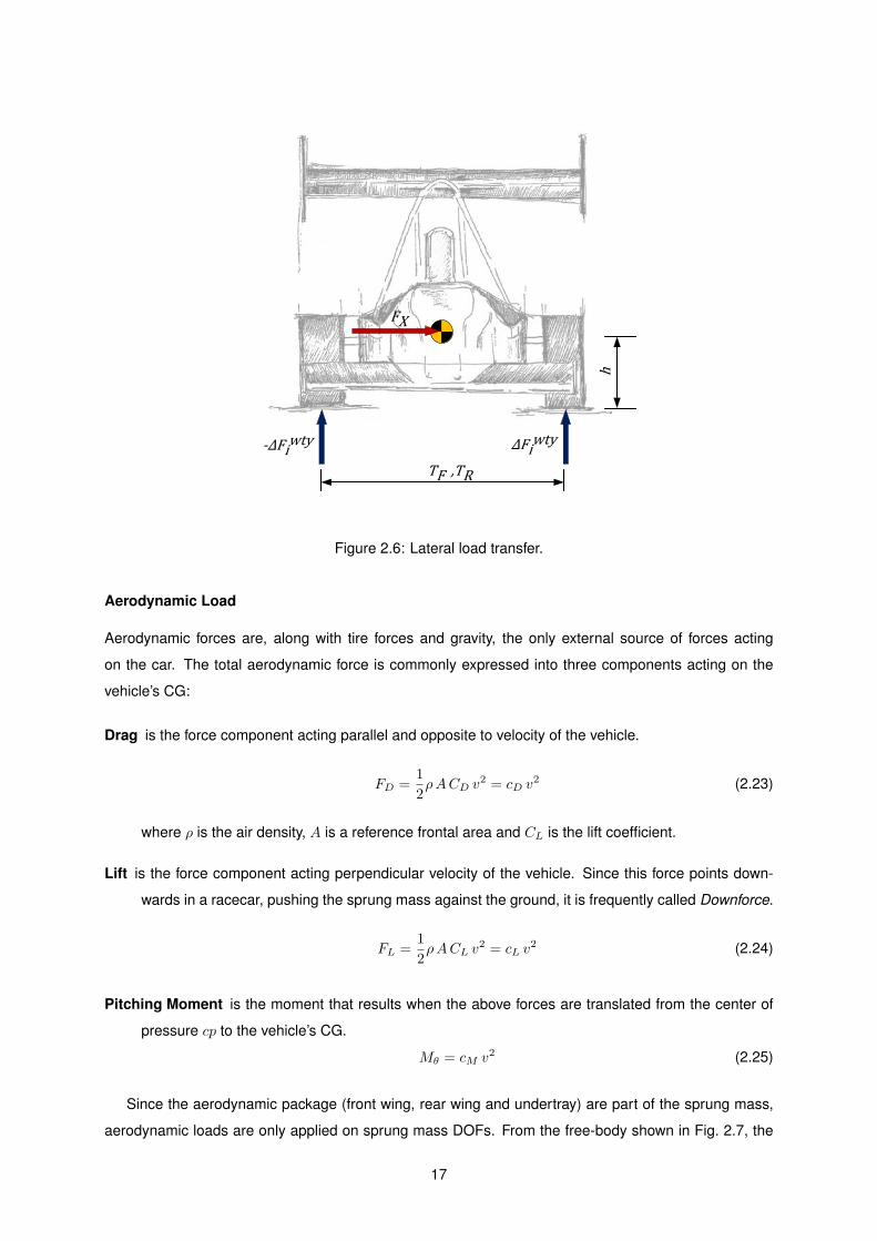
Lateral load transfer is similarly calculated from the free-body diagram in Fig. 2.6.
∆Fwtys,F = ms aYb
L
hsTF
(2.21a)
∆Fwtys,R = ms aYa
L
hsTR
(2.21b)
15

L
ba
FX
2ΔFF wtx -2ΔFR
wtx
h
Figure 2.5: Longitudinal load transfer.
∆Fwtyu,F = mu,F aYhuTF
(2.21c)
∆Fwtyu,R = mu,R aYhuTR
(2.21d)
The total load change due to weight transfer is, respectively, for each corner of the sprung and
unsprung masses:
∆Fwts,FL = −∆Fwtxs
2−∆Fwtys,F (2.22a)
∆Fwts,FR = −∆Fwtxs
2+ ∆Fwtys,F (2.22b)
∆Fwts,RL =∆Fwtxs
2−∆Fwtys,R (2.22c)
∆Fwts,RR =∆Fwtxs
2+ ∆Fwtys,R (2.22d)
∆Fwtu,FL = −∆Fwtxu
2−∆Fwtyu,F (2.22e)
∆Fwtu,FR = −∆Fwtxu
2+ ∆Fwtyu,F (2.22f)
∆Fwtu,RL =∆Fwtxu
2−∆Fwtyu,R (2.22g)
∆Fwtu,RR =∆Fwtxu
2+ ∆Fwtyu,R (2.22h)
16
TF ,TR
FX
-ΔFiwty ΔFi
wty
h
Figure 2.6: Lateral load transfer.
Aerodynamic Load
Aerodynamic forces are, along with tire forces and gravity, the only external source of forces acting
on the car. The total aerodynamic force is commonly expressed into three components acting on the
vehicle’s CG:
Drag is the force component acting parallel and opposite to velocity of the vehicle.
FD =1
2ρACD v
2 = cD v2 (2.23)
where ρ is the air density, A is a reference frontal area and CL is the lift coefficient.
Lift is the force component acting perpendicular velocity of the vehicle. Since this force points down-
wards in a racecar, pushing the sprung mass against the ground, it is frequently called Downforce.
FL =1
2ρACL v
2 = cL v2 (2.24)
Pitching Moment is the moment that results when the above forces are translated from the center of
pressure cp to the vehicle’s CG.
Mθ = cM v2 (2.25)
Since the aerodynamic package (front wing, rear wing and undertray) are part of the sprung mass,
aerodynamic loads are only applied on sprung mass DOFs. From the free-body shown in Fig. 2.7, the
17

load change due to aerodynamic forces is given by:
L
ba
FD
2ΔFF aero -2ΔFR
aero
h
FL
CP
MA
Figure 2.7: Aerodynamic load.
∆F aeros,FL = ∆F aeros,FR =−FD hs + FL b−Mθ
2L(2.26a)
∆F aeros,RL = ∆F aeros,RR =FD hs + FL a+Mθ
2L(2.26b)
2.3.3 Inverse Kinematics
Since the available parameter values are taken from the static deflection state, i.e., measured when the
car is stationary and loaded only with its own weight (static load), the vibrational model is excited solely
with dynamic loads, i.e., the external forces on vector {F} (Eq. 2.18) are given by:
Fs,i = ∆Fwts,i + ∆F aeros,i (2.27a)
Fu,i = ∆Fwtu,i (2.27b)
Equation 2.14 is numerically solved in order of q, using previous time-step values for q and q.
{q} = [M]−1(
[F ]− [C] {q} − [K] {q})
(2.28)
18

or, in the discrete difference form
qi((k + 1)Ts) = [M]−1(
[F(kTs)]− [C] qi(kTs)− [K] qi(kTs))
(2.29)
Velocity and position can then be calculated through integration over time.
q(t) =
∫q(τ)dτ (2.30a)
q(t) =
∫q(τ)dτ (2.30b)
2.3.4 Tire Vertical Load
Static load is then added to the transient load retrieved from the model to get the total tire load.
Total tire vertical load is the sum of the static loads and the transient load retrieved from the vibrational
model, as a reaction force on the road for zr,i = zr = 0:
FZT,i = F sts,i + F sts,i + cT .zu,i + kT .zu,i (2.31)
Therefore, vertical dynamics yield the tire vertical loads as a function of the vehicle acceleration and
velocity vectors.
FZT,i = f(Fs,i, Fu,i) = f(aX , aY , vX , vY ) (2.32)
2.4 Wheel Dynamics
The dynamics of the wheel under braking are one of the most important areas in Vehicle Dynamics when
developing an ABS controller. As described in the beginning of this chapter, Wheel Dynamics deal with
the sum of forces and moments acting on the wheel to calculate the angular velocity of the whell ωW .
With the knowledge of the vehicle velocity, Wheel Dynamics ultimately calculates and outputs the actual
longitudinal slip ratio SX , necessary for the Tire Model.
2.4.1 Free-body diagram
The free-body diagram shown in Fig. 2.8 yields the following equations:
m
4vX = FXT (2.33)
IW ωW = TW −RLFXT (2.34)
19

Figure 2.8: Freebody diagram of the wheel.
where the wheel torque TW can be positive or negative, either this comes from the motor or the brakes.
TW = Td, if TW > 0 (Driving Torque)
TW = Tb, if TW < 0 (Braking Torque)(2.35)
Longitudinal tire forces FXT , as described in the next chapter, depend on the longitudinal slip ratio
SX . Its calculation, though part of the Wheel Dynamics, is addressed later in Section 4.3.1.
2.5 Brakeline Dynamics
Brakeline refers to the mechanical and hydraulic systems that transform the force applied on the brake
pedal Fbp into a brake torque Tb exerted by the calipers on each wheel. These include the brake pedal,
master cylinders, brake lines, wheel calipers and rotors. In the absence of an ABS controller, brakeline
components can be divided as depicted in Fig. 2.9.
Figure 2.9: Schematic of basic brakeline dynamics.
20

2.5.1 Steady-state equations
Brake pedal acts as a lever that multiplies Fbp by a geometric constant designated as Pedal Ratio, PR.
The resultant force is distributed to the master cylinders responsible for the front and rear brake lines,
according to the brake bias BB (equations 2.36).
Fmc = Fbp ∗ PR (2.36a)
Fmc,F = Fmc ∗ BBF (2.36b)
Fmc,R = Fmc ∗ BBR (2.36c)
Assuming an incompressible a brake fluid and ideal efficiency for brakeline components, pressure is
kept constant:
pmc = pcal = p =FmcAmc
=FcalAcal
(2.37)
Thus, the relation between the force on the master cylinder piston and the force exerted on caliper
pistons is given by the squared inverse of the ratio between its diameters:
Fcal = FmcAcalAmc
= Fmc
(dcaldmc
)2
(2.38)
The hydraulic pressure translated into mechanical force by the caliper is then applied on a couple of
brake pads, one on each side of the rotor, so a clamping force is generated. With the knowledge of the
coefficient of friction between the brake pads and the rotor, µpads, brake torque is finally calculated.
Fpads = 2Fcal (2.39a)
Tb = FbRb = µpads FpadsRb (2.39b)
where Rb designates the effective brake radius, the distance between the rotor center and the center of
pressure of the caliper pistons.
Introducing equations 2.38 and 2.39 on Eq. 2.36a, brake torque becomes a linear function of the
brake pedal force:
Tb = f(Fbp) = 2µpads
[PR
(dcaldmc
)2]· Fbp ·Rb
= K · Fbp = 1.02 · Fbp
(2.40)
21
2.5.2 Transient behaviour
For most applications, the response characteristics of hydraulic brake systems are such that the time
lags between input and output variables are very small, typically less than 0.5 s [12]. However, when
it comes to ABS design, the dynamic response of an hydraulic brake system and its individual brake
components becomes important [11].
The main dynamic elements in a typical brake system are the brake lines. The flow of brake fluid
from the master cylinder to the wheel cylinder is a function of fluid viscosity, cross-sectional flow area,
and brake line length [11]. As fluid viscosity increases, the time interval between the application of force
to the brake pedal and operation of the wheel brake increases and may affect the performance of an
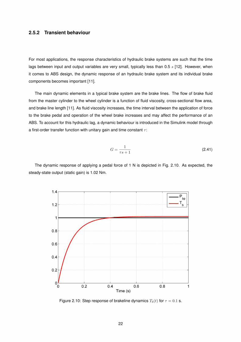
ABS. To account for this hydraulic lag, a dynamic behaviour is introduced in the Simulink model through
a first-order transfer function with unitary gain and time constant τ :
G =1
τs+ 1(2.41)
The dynamic response of applying a pedal force of 1 N is depicted in Fig. 2.10. As expected, the
steady-state output (static gain) is 1.02 Nm.
Figure 2.10: Step response of brakeline dynamics Tb(t) for τ = 0.1 s.
22

2.5.3 Hydraulic Modulator
A hydraulic pressure modulator is an electro-hydraulic device for reducing, holding, and restoring the
pressure within a hydraulic circuit. It forms the hydraulic link between the brake master cylinder and the
wheel-brake cylinders (see Figures 2.11 and 4.2) and is essential for any ABS application.
Figure 2.11: Schematic of brakeline dynamics with hydraulic modulator.
The pressure is regulated by an ECU that sends a control signal for energizing one or both inlet and
outlet solenoid valves, according to Table 2.2. The maximum pressure is determined by the pressure
on the master cylinder. Depending on the design, this device may also include a pump/motor assembly,
accumulator and reservoir, as depicted in Fig. 2.12.
Mode Inlet Valve (State) Outlet Valve (State)
Increase/Restore Open (0) Closed (0)
Hold Closed (1) Closed (0)
Decrease Closed (1) Open (1)
Table 2.2: Hydraulic modulator solenoid valves.
Figure 2.12: Schematic of a hydraulic modulator [3].
Hyraulic modulator valve positions work as described here:
Open When the valve is open, pressure from the master cylinder is free to pass through the brake
circuit. In this condition, the amount of brake pressure is directly controlled by the driver.
23
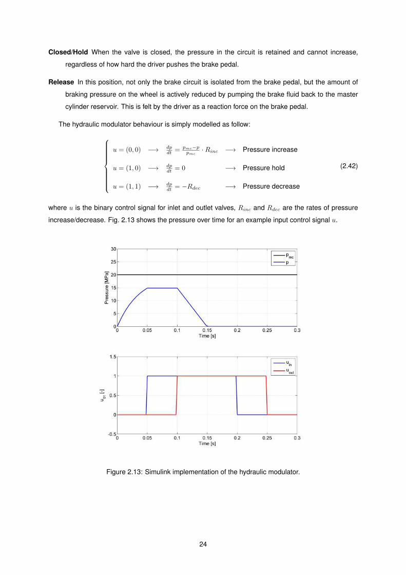
Closed/Hold When the valve is closed, the pressure in the circuit is retained and cannot increase,
regardless of how hard the driver pushes the brake pedal.
Release In this position, not only the brake circuit is isolated from the brake pedal, but the amount of
braking pressure on the wheel is actively reduced by pumping the brake fluid back to the master
cylinder reservoir. This is felt by the driver as a reaction force on the brake pedal.
The hydraulic modulator behaviour is simply modelled as follow:
u = (0, 0) −→ dpdt = pmc−p
pmc·Rinc −→ Pressure increase
u = (1, 0) −→ dpdt = 0 −→ Pressure hold
u = (1, 1) −→ dpdt = −Rdec −→ Pressure decrease
(2.42)
where u is the binary control signal for inlet and outlet valves, Rinc and Rdec are the rates of pressure
increase/decrease. Fig. 2.13 shows the pressure over time for an example input control signal u.
Figure 2.13: Simulink implementation of the hydraulic modulator.
24

Chapter 3
Tire Model
Tires are the primary source of the tractive, braking, and cornering forces/torques that provide the han-
dling and control of a car. For that reason, they are one of the most important components and its
understanding in respect of the magnitude, direction and limit of those forces/torques is essential for any
application in vehicle dynamics and/or vehicle control system. However, the complexity of tire behaviour
is not yet completely understood — even in professional motorsports they’re often known as ‘black magic’
— and the development of model for all driving conditions in real-time is still a very challenging task.
In this chapter, three tire models are described: two semi-empirical models, Pacejka (Section 3.1.1)
and Burkhardt (Section 3.1.2); and ANN-based model (Section 3.1.3. The models are then used to
fit the experimental data (illustrated in Section 3.2), whose methodology is described and results are
compared (Section 3.3).
3.1 Types of models
Several tire models can be found in the literature. Depending on how one approaches the problem,
models can be classified between theoretical and empirical (Fig. 3.1).
From experimental data only
Using similarity methods
Through simple physical model
Through complex physical model
Empirical Theoretical
Figure 3.1: Classification of tire models.
25

Nevertheless, the objective of every model is to output the tire horizontal forces and/or moments as
a function of one or more rolling conditions: tire vertical load, longitudinal slip ratio, slip angle, inclination
angle, temperature, pressure and so on.
[FXT , FY T ,MXT ,MY T ,MZT ] = f(FZT , SX , α, γ, T, p, . . .) (3.1)
3.1.1 Pacejka Model
Pacejka1 tire model [13] is the most widely used tire model to calculate steady-state tire force and
moment characteristics for use in vehicle dynamics. As a semi-empirical model, it is particulary useful
to represent the tire as a vehicle component in a vehicle simulation environment, as in this work. This
model is classified as ’semi-empirical’ because, despite being based on measured data, it contains
structures that find their origin in physical models like the brush model.
Pacejka tire model is given by the parametric equation, known as MF:
y = D sin [C arctan {Bx− E (Bx− arctanBx)}]
Y (X) = y(x) + SV
x = X + SH
(3.2)
where Y is the output variable FXT , FY T or MZT and x is the main x-axis input variable, namely tanα or
SX . The remaining parameters listed in Table 3.1 represent geometric characteristics of the MF curve,
as shown in Fig. 3.2.
B stiffness factor
C shape factor
D peak value
E peak value
SH horizontal shift
SV vertical shift
Table 3.1: Magic Formula coefficients
When multiple inputs are needed for the tire model (e.g., varying tire vertical load and road coefficient
of friction is important for this application), the aforementioned parameters are itself given by parametric
functions (of parameters pi, qi, ri or si) whose inputs are the supplementary input variables FZT , γ and
p. The actual expressions for these functions differ depending on the type of tire data to be fitted:
• Longitudinal Force for pure longitudinal slip, FXT = f(SX , α = 0◦)
• Lateral Force for pure side slip, FY T = f(SX = 0 , α)1Hans Bastiaan Pacejka (Rotterdam, 1934), Professor emeritus at Delft University of Technology in Delft, Netherlands, is an
expert in vehicle system dynamics and particularly in tire dynamics, fields in which his works are now standard references.
26
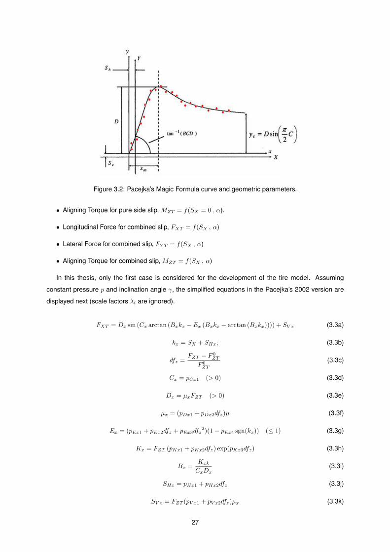
Figure 3.2: Pacejka’s Magic Formula curve and geometric parameters.
• Aligning Torque for pure side slip, MZT = f(SX = 0 , α).
• Longitudinal Force for combined slip, FXT = f(SX , α)
• Lateral Force for combined slip, FY T = f(SX , α)
• Aligning Torque for combined slip, MZT = f(SX , α)
In this thesis, only the first case is considered for the development of the tire model. Assuming
constant pressure p and inclination angle γ, the simplified equations in the Pacejka’s 2002 version are
displayed next (scale factors λi are ignored).
FXT = Dx sin (Cx arctan (Bxkx − Ex (Bxkx − arctan (Bxkx)))) + SV x (3.3a)
kx = SX + SHx; (3.3b)
dfz =FZT − F 0
ZT
F 0ZT
(3.3c)
Cx = pCx1 (> 0) (3.3d)
Dx = µxFZT (> 0) (3.3e)
µx = (pDx1 + pDx2dfz)µ (3.3f)
Ex = (pEx1 + pEx2dfz + pEx3dfz2)(1− pEx4 sgn(kx)) (≤ 1) (3.3g)
Kx = FZT (pKx1 + pKx2dfz) exp(pKx3dfz) (3.3h)
Bx =Kxk
CxDx(3.3i)
SHx = pHx1 + pHx2dfz (3.3j)
SV x = FZT (pV x1 + pV x2dfz)µx (3.3k)
27

3.1.2 Burkhardt Model
Burkhardt tire model [14] is a static parametric model given by the following velocity-dependent para-
metric expression:
F (x) =[A(1− e−Bx
)− Cx
]e−Dxv (3.4)
where (F, x) is any of the following combinations: (FXT , SX), (FY T , α) or (MZT , α).
Although this model takes into account the influence of the vehicle velocity v on the friction curve,
there is no dependency on the tire vertical load FZT or inclination angle γ. For that reason, a given set
of coefficients only applies for a given set of rolling conditions.
3.1.3 Neural Network Model
Inspired by biological nervous systems, artificial neural network (ANN) is a network structure consisting
of a number of parametric nodes connected through directional links defining a causal relationship them.
The outputs of each node, and thus the output of the network, on the adaptable values of the node’s
parameters. A learning rule specifies how these parameters should be updated to minimize a prescribed
error measure between the network’s actual output and a desired output [15].
Figure 3.3: Artificial neural network (ANN) scheme.
Trying to take advantage of the effectiveness of ANN for nonlinear curve fitting, a tire model has been
developed using this type of soft-computing algorithm. A model of this kind is not only relatively fast to
develop, it also allows the use of any mapping combination of variables as in the Pacejka tire model
(e.g., FXT = f(SX , FZT ), or {FXT , FY T } = f(SX , α, FZT )).
28
3.2 Experimental Data
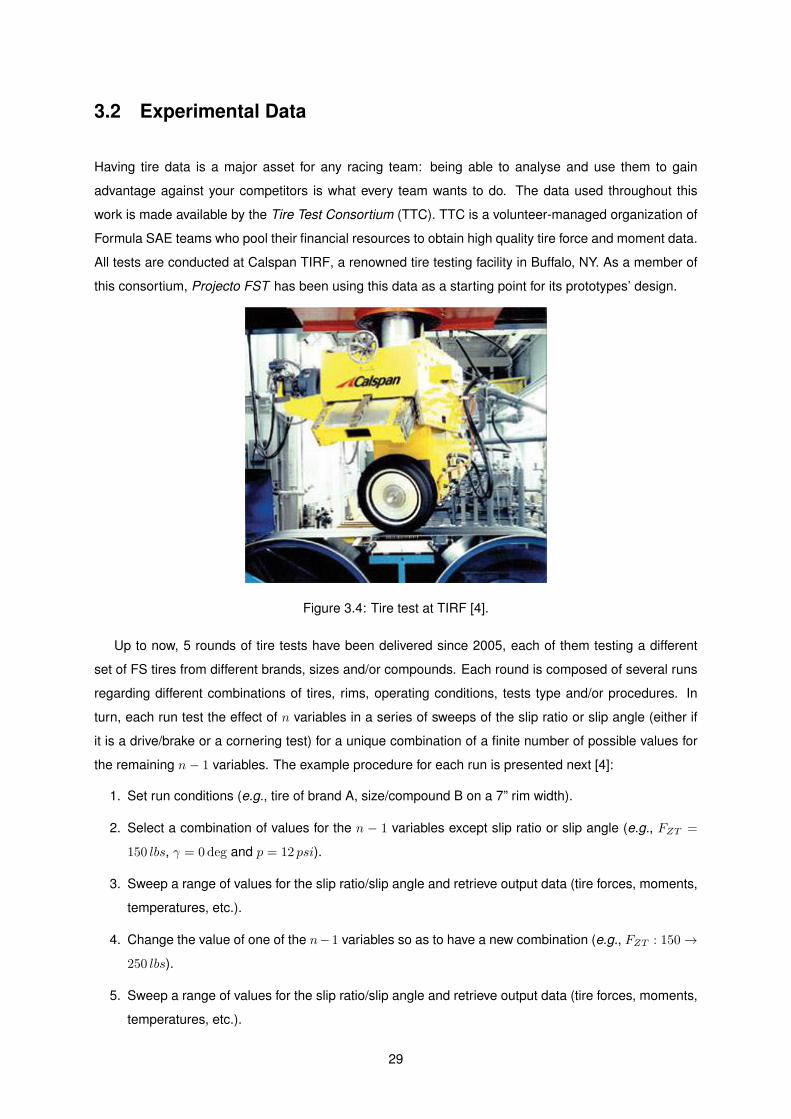
Having tire data is a major asset for any racing team: being able to analyse and use them to gain
advantage against your competitors is what every team wants to do. The data used throughout this
work is made available by the Tire Test Consortium (TTC). TTC is a volunteer-managed organization of
Formula SAE teams who pool their financial resources to obtain high quality tire force and moment data.
All tests are conducted at Calspan TIRF, a renowned tire testing facility in Buffalo, NY. As a member of
this consortium, Projecto FST has been using this data as a starting point for its prototypes’ design.
Figure 3.4: Tire test at TIRF [4].
Up to now, 5 rounds of tire tests have been delivered since 2005, each of them testing a different
set of FS tires from different brands, sizes and/or compounds. Each round is composed of several runs
regarding different combinations of tires, rims, operating conditions, tests type and/or procedures. In
turn, each run test the effect of n variables in a series of sweeps of the slip ratio or slip angle (either if
it is a drive/brake or a cornering test) for a unique combination of a finite number of possible values for
the remaining n− 1 variables. The example procedure for each run is presented next [4]:
1. Set run conditions (e.g., tire of brand A, size/compound B on a 7” rim width).
2. Select a combination of values for the n − 1 variables except slip ratio or slip angle (e.g., FZT =
150 lbs, γ = 0 deg and p = 12 psi).
3. Sweep a range of values for the slip ratio/slip angle and retrieve output data (tire forces, moments,
temperatures, etc.).
4. Change the value of one of the n−1 variables so as to have a new combination (e.g., FZT : 150→250 lbs).
5. Sweep a range of values for the slip ratio/slip angle and retrieve output data (tire forces, moments,
temperatures, etc.).
29

6. If all combinations have been tested, stop run. Else, return to step 4.
Figure 3.5 shows the value of 5 variables during a complete example drive/braking run. As described,
there is SX sweep for each one of the possible combinations of the other 4 variables, α, FZT , γ and p, as
a series of for -cycles. In red is highlighted a sample of data for FZT = {50, 150, 250, 350} lbs, α = γ = 0◦
and p = 69 kPa (10 psi). The output FXT of these data is plotted over SX in Fig. 3.6.
Figure 3.5: Data from a complete run. In red, data sample for FZT = {50, 150, 250, 350} lbs, α = γ = 0◦
and p = 69 kPa (10 psi).
30

Figure 3.6: Plot of SX vs. FXT for four sweeps of different FZT .
3.3 Data Fitting
Depending on the model, so depends methodology used for fitting the experimental data. Hence,
Pacejka and Burkhardt models make use an optimization technique that computes the model param-
eters that minimize the error to the real data.
Neural Network model fitting is achieved by network training using MATLAB’s Neural Network toolbox.
3.3.1 Methodology for Pacejka and Burckhardt models
The development of the empirical models described before is related with the estimation of the set of
coefficients pi for the Pacejka Model and the coefficients [A,B,C,D] that best fit the TTC data shown
in Section 3.2. It is therefore an optimization or nonlinear regression problem that is adressed using the
least squares method approach.
31

Least Squares Method
The best fit in the least squares sense is the column vector of parameters p = pi that minimizes the sum
of the squared residuals, i.e., the difference between an experimental value and the fitted value provided
by a model.
minp
∑i
r2i =
∑i
(F (p, xi)− yi)2 (3.5)
In MATLAB, this problem is solved using either the Curve Fitting Toolbox or the lsqcurvefit function
with the parameters listed in Table 3.2. To avoid the algorithm to get ‘stucked’ in local minima or take too
much iterations, a set of Pacejka and Burkhardt parameters is given by [13] and [16], respectively, and
used as starting point.
Algorithm Levenberg-Marquardt
TolFun 1× 10−6
TolX 1× 10−6
MaxIter 1× 10⁻⁶
Others default
Table 3.2: MATLAB’s lsqcurvefit parameters [1].
3.3.2 Results
Pacejka
Figure 3.7 plots the sample TTC data from Fig. 3.6 and the final optimized MF curve. As expected, a very
good fit is achieved for every FZT . Moreover, the structure of Eqs. 3.3 ensure that model extrapolation
beyond |SX | > 0.2, for which no experimental data is available, is relatively accurate, at least qualitatively
[13].
Burkhardt
Since the Burkhardt model does not allow a change in the rolling conditions, Eq. 3.4 can only fit a single
TTC sweep of SX . For FZT = 350 lbs, α = 0◦, γ = 0◦ and p = 14 psi, Fig. 3.8 shows the achieved fit. As
in the Pacejka model, the parametric expression defining the Burkhardt model (Eq. 3.4) is specific to tire
fitting, thus qualitatively correct. However, poor fitting on the limits of the experimental data suggest that
extrapolation is not advised in this case.
Nonetheless, using the same values for the coefficients [A,B,C,D], Burkhardt model is useful for
reproducing the influence of the velocity on the tire force. As expected from [17], Fig. 3.8 shows that the
peak value of FXT decreases for higher velocities.
32

−0.5 −0.4 −0.3 −0.2 −0.1 0 0.1 0.2 0.3 0.4 0.5−4,000
−3,000
−2,000
−1,000
0
1,000
2,000
3,000
4,000
SX
FX
T(N
)
FZT = 350 lbsFZT = 150 lbsFZT = 250 lbsFZT = 50 lbs
Figure 1.7: Pacejka Model vs. TTC Data for FZT = {50, 150, 250, 350} lbs.
9
Figure 3.7: Pacejka Model vs. TTC Data for FZT = {150, 250, 350} lbs.
Figure 3.8: Burkhardt Model vs TTC Data for different velocities.
33

Neural Network
After several iterations of different trained ANN, the network with the best fit was selected. Figure 3.9
shows the same experimental shown in Fig. 3.6 (also used for the Pacejka model fitting) and the fitted
Neural Network model. As in the Pacejka model, a very good fit is achieved for the experimental.
However, network outputs are not valid for SX values outside the experimental range.
Figure 3.9: Neural Network Model vs. TTC Data for FZT = {150, 250, 350} lbs.
Comparison
Considering the results achieved with the three tire models, a decision has been made on the Pacejka
model to be coupled with the full vehicle model for design and simulation of the ABS controller. In fact,
it is the only model that ensures accuracy within the complete range of possible SX values, with special
importance for the wheel-lock case SX = −1 (see Section 4.3.1). Mean squared error (MSE) results for
the three models are summarized in Table 3.3.
Model MSE
Pacejka 9594 N2
Burkhardt 26477 N2
NN (global) 8706 N2
Table 3.3: MSE fitting result for Pacejka, Burkhardt and Neural Network tire models.
34

Chapter 4
ABS Overview
This chapter gives a further overview of the ABS. It starts by outlining the ABS objectives (Section 4.1)
and describing its main components (Section 4.2). Afterwards, the problem of wheel slip control is
defined from the control theory point of view (Section 4.3), along with the definition of the longitudinal
slip ratio SX (Section 4.3.1). The chapter ends with a literature review on the more relevant control
methods (Section 4.4).
4.1 Objectives of ABS
Modern ABSs has three main goals that must be fulfilled, regardless of the application, system architec-
ture or the chosen control algorithm:
Stopping Distance By maximizing the longitudinal frictional force under braking the stopping distance
will be minimized, for the same vehicle mass m and initial velocity v0.
dbraking = − v2i
2 · aXwhere aX =
FX(µ)
m(4.1)
Stability Achieving the maximum friction level on all four wheels is not always desirable, specially for
sudden and uneven changes on the surface µ. Significant asymmetries between right and left side
braking forces result on a yaw moment and consequent vehicle instability, as depicted by Fig. 4.1.
Therefore, the ABS must keep balanced braking forces, even if total force is not maximized.
Steerability Available lateral friction force decays with wheel slip towards lock-up. To ensure steerability
during braking, the ABS should be able to maintain enough lateral friction force.
35

Figure 4.1: Buildup of yaw moment induced by large differences in friction coefficients [5].
4.2 ABS Components
A typical ABS comprises a series of subsystems interconnected in a control loop (figures 4.2 and 4.4).
The main components of an ABS are described next:
Figure 4.2: ABS components diagram.
Electrical control unit (ECU) Usually microprocessor-based, it is the core component that receives,
filters and amplifies the signal from the sensors and performs the necessary calculations for ve-
hicle velocity and wheel slip estimation. The ECU then sends a signal to the hydraulic modulator
according to the implemented control algorithm.
36

Hydraulic Modulator An electro-hydraulic device that, depending on the control signal from the ECU,
is able to increase, hold or decrease the brakeline pressure downstream to the wheel calipers, by
energizing a couple of solenoid valves. The hydraulic modulator is described in more detail and
modelled in Section 2.5.3 as part of the Brakeline Dynamics.
Sensors These are connected with the ECU an provide feedback measurements of the rotational veloc-
ity of all wheels (normally an inductive or Hall-effect encoder mounted on the hub), brake pressure
and acceleration (accelerometer on the CG).
4.3 Wheel Slip Control
From Section 4.1, all ABS objectives rely on keeping tire longitudinal and lateral friction forces, FXT and
FY T , at desired levels. As described earlier in Chapter 3, these forces depend, among other variables,
on the value of the wheel slip SX .
{FXT , FY T } = f(SX , . . .) (4.2)
Before any formalization of the control problem, the mathematical concept of wheel slip or longitudinal
slip ratio SX is formally introduced in the next section.
4.3.1 Longitudinal Slip Ratio
A loaded tire is considered to be rolling freely if neither a driving nor a braking torque is applied (assuming
a linear path, zero slip angle and zero inclination angle). In this condition, the tire longitudinal velocity
and the vehicle longitudinal velocity are equal. In this conditions, a reference wheel-spin velocity can
thus be defined as:
ωW0 =vXRe
(4.3)
where Re is the so-called effective rolling radius [13]. For simplification purposes, this will be considered
constant and equal to the tire loaded radius RL.
dRedt
= 0
Re(t) = RL
(4.4)
When a torque is applied about the wheel-spin axis, tire deformation is generated and causes a slip
to arise between the tire and the road [13]. This means that the actual wheel-spin velocity or wheel
37

angular velocity ωW is different from the reference wheel-spin velocity, i.e., the wheel and the vehicle
have different longitudinal velocities.
ωW 6= ωW0 ⇔ ωW .RL 6= vX (4.5)
The difference between these velocities is called the longitudinal slip velocity vs:
vs = ωW − ωW0 = ωW −vXRL
(4.6)
Finally, the ratio of longitudinal slip velocity to the reference wheel-spin velocity is formally defined
in [7] as the longitudinal slip ratio, or simply wheel slip SX :
SX =ωW − ωW0
ωW0=ωWRe − vX
vX(4.7)
According to Eq. 4.7, to following situations may occur:
ωW � ωW0 ⇔ SX →∞ −→ Wheel is ‘spinning’
ωW > ωW0 ⇔ SX > 0 −→ Tire driving force (FXT > 0)
ωW = ωW0 ⇔ SX = 0 −→ Free-rolling tire (FXT = 0)
ωW < ωW0 ⇔ SX < 0 −→ Tire braking force (FXT < 0)
ωW = 0 ⇔ SX = −1 −→ Wheel lock-up
(4.8)
When the car stops ωW = vX = 0, which leads to the mathematical indetermination 00 . To avoid the
consequent computacional error the denominator is replaced by max(vX , ε) in the Simulink R© environ-
ment, where ε ≡ eps = 2−52 (double-precision floating-point relative accuracy [1]).
4.3.2 Control Problem Definition
Recalling a typical tire friction curve from Chapter 3, fulfilling the ABS objectives means that the longitu-
dinal slip ratio SX should be kept within a range so that longitudinal and lateral friction are near its peak
values (Fig. 4.3). Hence, the ABS control problem is inherently related with the control of wheel slip. As
the optimum value of SX do not coincide for both FXT and FY T , a compromise is frequently necessary.
In practical terms, since vehicle speed vX cannot be directly controlled, wheel slip control is executed
by controlling wheel angular velocity ωW alone, which in turn is accomplished by manipulating the brake
pressure on the wheel caliper pcal. The complete set of closed-loop variables for wheel slip control is
listed in Table 4.1. Disturbances in the control loop may refer to, e.g. changes in the road conditions
(road profile zr, coefficient of friction µ), sensor noise w and others.
38

0− 0.04− 0.08− 0.12− 0.16− 0.20− 0.24− 0.28− 4,000
− 3,500
− 3,000
− 2,500
− 2,000
− 1,500
− 1,000
− 500
0
SX
FT
(N)
FXT(µ = 0.65, Pacejka)FXT(µ = 0.65, TTC)FXT(µ = 0.2, Pacejka)FYT(α = − 6o, TTC)
UnstableRegion
StableRegion
SXref
Region
Figure 4.3: ABS action zones.
Figure 4.4: ABS control loop components [5]: 1-Hydraulic Modulator, 2-Master Cylinder, 3-Wheel caliper,4-ECU.
39

Object variable SX Longitudinal slip ratio
Controlled variable ωW Wheel speed
Reference variable SrefX Reference longitudinal slip ratio
Manipulated variable pb Braking pressure
Disturbances zr, µ, w . . . Road conditions, sensor noise, etc.
Table 4.1: Closed-loop variables for wheel slip control.
4.3.3 Main difficulties
The main difficulties in the design of any ABS control arise the strong nonlinearity and uncertainty of the
system to be controlled, namely:
• The interaction between the tire and the road surface is a very complex and hardly understood
area of knowledge. Friction models like the ones described in Chapter 3 are experimental-based
approximations of highly nonlinear phenomena.
• The dynamics of the whole vehicle are nonlinear and may even vary over time. Additionally, mod-
els often have to deal with a certain amount of parametric or structural uncertainty (e.g. vehicle
parameters, differential exactitude, model simplifications, etc.).
• ABS control requires significant robustness to deal with the previous uncertainties and variations
that are likely to happen, e.g., changes of vehicle loading, unknown and changeable road condi-
tions, components wear, sensor noise.
• Vehicle velocity, essential for wheel slip calculation, and road coefficient of friction µ are hard
and expensive to measure directly. Reliable ABS performance depend on good estimates of this
variables.
• ABS actuators are discrete and control precision must be achieved with only three types of control
commands: build pressure, hold pressure or reduce pressure (see Section 4.2).
Another meaningful aspect is the fact that the system is unstable for wheel slip values beyond the
peak friction force seen in Fig. 4.3. Since longitudinal force diminishes from this point on, an increase in
wheel slip leads to a decrease in the reaction torque exerted by the road to counteract the brake torque,
thus continuously increasing wheel slip towards lock-up.
40

4.4 Control Methods
From the detailed issues discussed above, wheel slip control is, indeed, a very complex and challenging
problem. Several approaches and constant improvements are still being released in newer versions of
ABSs. The predominant control methods existing in the literature can be categorized in four different
areas:
• Threshold control
• PID control
• Sliding-mode control (SMC)
• Intelligent control
The most relevant applications of each control method are reviewed in the next subsections.
4.4.1 Threshold Control
Threshold control is a simple control method that has been widely applied in the early ABS versions.
Generic threshold algorithm usually uses wheel acceleration and/or wheel slip as controlled variables
and defines threshold values, above/below which the pressure should be increased, held or decreased.
A typical control cycle implemented by Bosch is described in [5] and uses three threshold values for
wheel acceleration (-a, +a and +A), as well as a slip-switching threshold (λ1) to manage pressure.
Control cycles with different threshold variables and criteria may also be used, with significant changes
on ABS performance, as tested and compared by Rangelov in [18].
Since the pressure is cyclically being increased, held and decreased based solely on binary states
of the input variables (Fig. 4.5), wheel speed oscillations over time are less controllable and ABS per-
formance is less effective than with other continuous control methods [19]. Nonetheless, as a simple
control algorithm, threshold control and its variants have been extensively applied in the literature over
the years. More recently, a four-wheel vehicle model with integrated vertical, horizontal, lateral and brak-
ing dynamics is used in [20] to evaluate the performance of a threshold ABS under various operating
conditions, with satisfactory results.
4.4.2 PID Control
Conventional PID is the most widely used control method in industry. Its simplicity makes it easy to
understand, design/tune and implement. It has been used for many years to successfully solve a diver-
sity of problems, from which ABS is no exception. Even for complex and changing surface types, good
results can be attained with conventional PID control algorithms [21].
41

Figure 4.5: ABS algorithm.
In the recent years, the well-known features of the conventional PID have been combined with the
robustness, self-tuning or adaptability to nonlinear models of other control methods, which highly en-
hanced ABS performance. A nonlinear PID control algorithm, similar to gain-scheduling algorithm, has
been applied in [22] to a class of truck ABS problems. Results show that ABS performance is increased
by adding robustness to the conventional PID. Lu et al designed a fuzzy PID controller combined with
a simple automatic optimization algorithm for PID parameters. This improved PID show better control
precision and robustness when compared with the conventional PID.
4.4.3 Sliding-mode Control
Sliding-mode control (SMC) is a form of robust control that provides an effective method to control
nonlinear plants. It consists of a sliding surface where a predefined function of error is zero, which
models the desired closed-loop performance; and a control law, such that the system state trajectories
are forced toward the sliding surface. Once the sliding surface is reached, the system state trajectories
should stay on it [23,24]. Due to the discontinuous switching of control force in the vicinity of the sliding
surface, SMC may, on the other hand, produce chattering effects which can cause system instability and
damage to both actuators and plants. In the development of SMC, the design of the sliding surface is of
significant importance, as it dictates the behaviour and performance of the overall control system [25].
A grey sliding-mode controller is designed by Kayacan et al [23] to maintain wheel slip at the desired
value. The proposed structure includes a grey predictor to anticipate the forthcoming velocity-dependent
values of wheel slip and the reference wheel slip. Simulation and experimental results that include sud-
den changes in road conditions indicate that the most attractive characteristic of a sliding-mode controller
is the robustness against the uncertainties in the system, such as noisy measurements or disturbances.
42

In [16], a sliding-mode controller is improved with integral switching surface to reduce chattering effects.
The robustness of the controller against nonlinearity and uncertainty is once again demonstrated by sim-
ulation results on a two-axle vehicle model. Patra et al proposes in [26] a recent sliding-mode controller
applied on a quarter car model with good slip tracking performance results. Yinggan Tang et al [27]
combine sliding mode controller with fractional order dynamics, in which fractional order proportional-
derivative (FOPD) sliding surface is adopted for faster track of the desired slip.
4.4.4 Intelligent Control
Intelligent control is an group of control techniques inspired on certain characteristics of intelligent bio-
logical systems. In fact, intelligent control frequently combines and extends theories and methods from
areas such as control, computer science, and operations research. It includes areas of knowledge like
artificial neural networks (ANNs), fuzzy logic, machine learning, evolutionary computation, or genetic
algorithms (GAs). Its resourcefulness allied to the continuous advances in computing technology allows
it to deal with increasingly broad and complex control problems.
On what concerns the ABS application, intelligent control has been an emerging and effective solu-
tion to deal with the nonlinear, uncertain and varying dynamics of braking process. An optimized fuzzy
controller is proposed by Mirzaei et al [3] to maintain the wheel slip on a desired level. Using genetic
algorithms and an error-based optimization approach for all parameters of a Takagi–Sugeno–Kang FIS,
very good performance and smoothness of the controller is achieved for a variety of road conditions. An
adaptive PID-type fuzzy control algorithm is designed in [6] for the ABS control. Experimental results
evidence that the performance of the ABS controller is increased by adding slip ratio estimation, optimal
slip ratio search and road condition identification mechanisms to the control scheme.
The integration of ANN on fuzzy controllers allows the inclusion of important adaptive and/or self-
tuning algorithms that may significantly increase ABS performance and robustness. A neuro-fuzzy
adaptive control approach for nonlinear dynamical systems is proposed by Topalov et al [28] and used
to design a wheel slip regulating controller. Raesian et al proposes in [29] an adaptive neuro-fuzzy
self-tuning PID control scheme to overcome the nonlinear dynamics. A hierarchical Takagi–Sugeno
fuzzy-neural model is used in [30] to develop a method for identification and robust adaptive control of
wheel slip integrated with an active suspension system.
Ultimately, GA provide a powerful optimization tool for the design of ABS controllers. As an exam-
ple, fuzzy and GAs are used in [31] to accomplish self-tuning on a PID control scheme and overcome
parameter variations and uncertainties and achieve the performance consistency.
43

44

Chapter 5
Proposed Approach
This chapter starts by outlining the available data and the design requirements (Section 5.1). A control
scheme is then proposed for the ABS (Section 5.2), including the selected control methods (Sections
5.2.1 and 5.2.2) based on the review included at the end of the previous chapter. Finally, the design
methodology for the following chapter is described (Section 5.3).
5.1 Problem data and requirements
Prior to any design decision, information regarding the prototype and the competition characteristics
should be taken into account and may affect the choice of the ABS control scheme. Moreover, there are
certain requirements with which the controller must comply, namely the competition rules.
5.1.1 FS Rules
Every FS competition must obey a set of rules defined by SAE International1. Beyond the main rules
whose purpose is to guarantee the safety of every member involved, including the pilot, team members,
organisational staff and public, the 2014 version of FSAE Rules 2 establishes a set of safety and technical
requirements that specifically concerns the brake system:
• The car must be equipped with a braking system that acts on all four wheels and is operated by a
single control.
• It must have two independent hydraulic circuits such that in the case of a leak or failure at any point
in the system, effective braking power is maintained on at least two wheels.
1Formerly the Society of Automotive Engineers, SAE International is a globally active professional association and standardsorganization for engineering professionals in various industries, namely automotive, aerospace and commercial-vehicle.
2Availabe at fsaeonline.com.
45
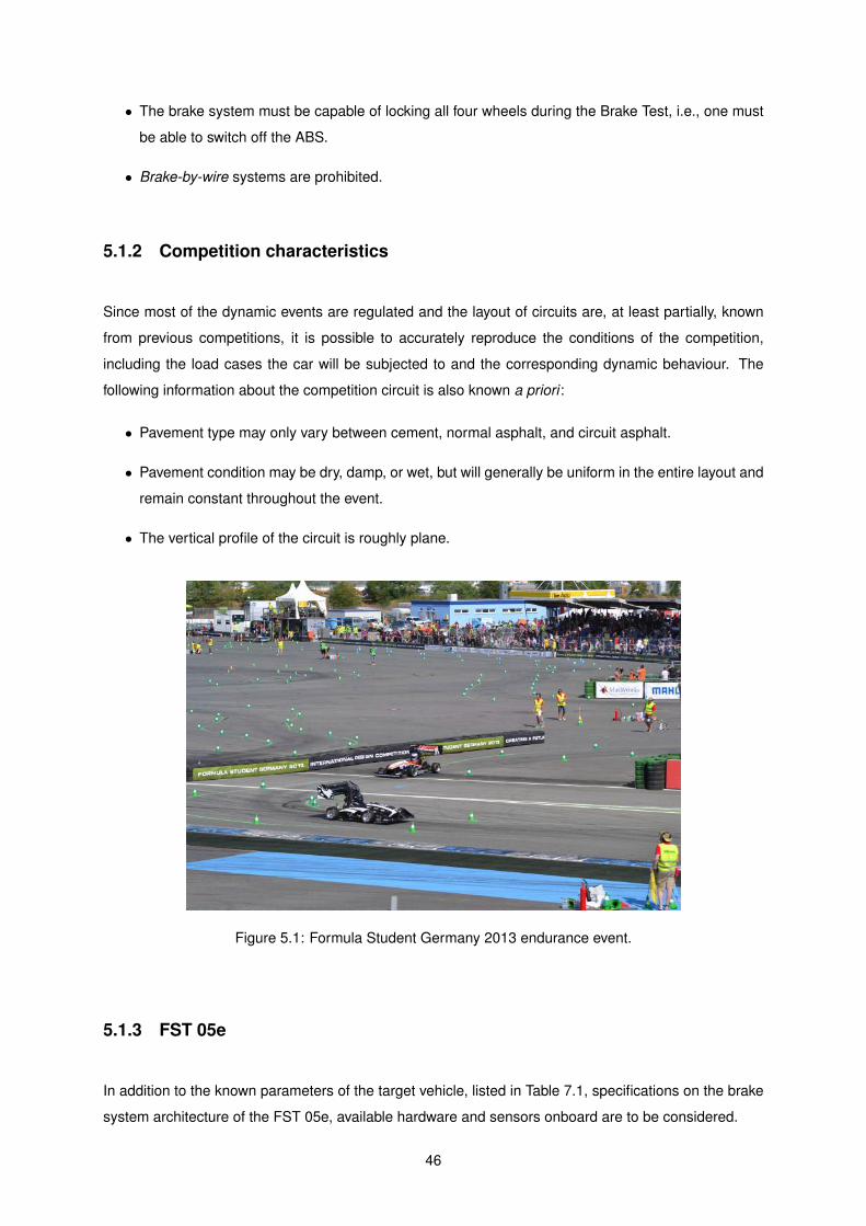
• The brake system must be capable of locking all four wheels during the Brake Test, i.e., one must
be able to switch off the ABS.
• Brake-by-wire systems are prohibited.
5.1.2 Competition characteristics
Since most of the dynamic events are regulated and the layout of circuits are, at least partially, known
from previous competitions, it is possible to accurately reproduce the conditions of the competition,
including the load cases the car will be subjected to and the corresponding dynamic behaviour. The
following information about the competition circuit is also known a priori :
• Pavement type may only vary between cement, normal asphalt, and circuit asphalt.
• Pavement condition may be dry, damp, or wet, but will generally be uniform in the entire layout and
remain constant throughout the event.
• The vertical profile of the circuit is roughly plane.
Figure 5.1: Formula Student Germany 2013 endurance event.
5.1.3 FST 05e
In addition to the known parameters of the target vehicle, listed in Table 7.1, specifications on the brake
system architecture of the FST 05e, available hardware and sensors onboard are to be considered.
46

Brake system architecture
The prototype has two independent hydraulic brake circuits for the front and rear wheels, respectively.
The brake pedal acts on the master cylinders, one for each circuit, and the hydraulic pressure is trans-
ferred through rigid brake lines to a floating caliper on each wheel. The calipers act on self-made brake
steel brake discs. Pressure distribution for the front and rear circuits (brake bias) is adjustable.
Available hardware and sensors
The following hardware and sensors are installed on the FST 05e prototype:
• Encoders for angular speed measurement in all 4 wheels;
• Three-dimensional accelerometer near the CG of the car;
• Pressure sensors for brakeline pressure, mounted on the wheel calipers;
• LVDT3 for linear travel measurement of the brake pedal.
5.2 Proposed Control Structure
For the ABS problem, a cascade control structure with two feedback loops is proposed and displayed
in Fig. 5.2. The main ABS controller, the wheel slip controller situated on the outer loop, compares the
actual wheel slip SX with a given reference and outputs a reference pressure prefb accordingly. This
reference pressure is then sent to a brake pressure controller, in the inner loop, which in turn sends a
command signal u to the hydraulic modulator (actuator) so the reference pressure is matched.
Additionally to the controllers, a wheel slip estimator is included in the outer loop. Having in mind the
physical implementation of the proposed structure, the estimator ensures an accurate estimation of the
wheel slip based on noisy measurements from the vehicle accelerometer and wheel speed encoders.
Figure 5.2: Proposed control structure.
Three types of blocks are depicted:
3Linear Variable Differential Transformer
47

Controller (red) Two controllers will be designed to track reference signals of brake pressure and wheel
slip. Further details on the chosen control methods are addressed in sections 6.1 and 6.2, respec-
tively.
Model (black) Contain the theoretical and experimental models built upon on the dynamic equations of
Chapter 2. Brake system is a representation of the brakeline dynamics alone (Section 2.5), whilst
the vehicle model includes the remaining horizontal, vertical and wheel dynamics, as well as the
tire model described in Chapter 3.
Estimator (blue) Include the aforementioned wheel slip estimator, described and designed in Sec-
tion 6.3.
This cascade arrangement means that the pressure controller deals only with the fast brakeline dy-
namics, allowing the wheel slip controller to exclusively deal with the slower remaining vehicle dynamics.
The combined effectiveness of the controllers is, thus, enhanced. Moreover, with this type of structure
the global ABS problem may be slip into several well-defined sub-problems, one for each loop, which
can be analysed and synthesized separately and systematically, as seen in Section 5.3.
5.2.1 Inner Loop - Brake Pressure Controller
The controller present in the inner loop should regulate the command signal ub sent to the hydraulic
modulator (Section 2.5.3) so that pressure on the caliper pcal matches the reference pressure prefb
determined by the slip controller in the outer control loop (Fig. 5.3).
Figure 5.3: Schematic of brakeline dynamics and pressure controller.
Object variable pcal Pressure on wheel caliper
Controlled variable pcal Pressure on wheel caliper
Reference variable pref Reference pressure
Manipulated variable p Brake line pressure
Disturbances wp, . . . Pressure sensor noise, etc.
Table 5.1: Closed-loop variables for pressure control.
The pressure controller has the following requirements:
48
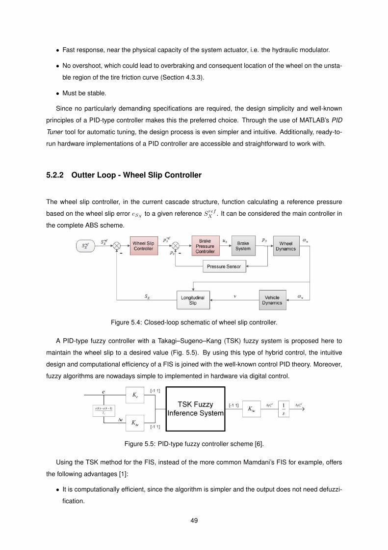
• Fast response, near the physical capacity of the system actuator, i.e. the hydraulic modulator.
• No overshoot, which could lead to overbraking and consequent location of the wheel on the unsta-
ble region of the tire friction curve (Section 4.3.3).
• Must be stable.
Since no particularly demanding specifications are required, the design simplicity and well-known
principles of a PID-type controller makes this the preferred choice. Through the use of MATLAB’s PID
Tuner tool for automatic tuning, the design process is even simpler and intuitive. Additionally, ready-to-
run hardware implementations of a PID controller are accessible and straightforward to work with.
5.2.2 Outter Loop - Wheel Slip Controller
The wheel slip controller, in the current cascade structure, function calculating a reference pressure
based on the wheel slip error eSX to a given reference SrefX . It can be considered the main controller in
the complete ABS scheme.
Figure 5.4: Closed-loop schematic of wheel slip controller.
A PID-type fuzzy controller with a Takagi–Sugeno–Kang (TSK) fuzzy system is proposed here to
maintain the wheel slip to a desired value (Fig. 5.5). By using this type of hybrid control, the intuitive
design and computational efficiency of a FIS is joined with the well-known control PID theory. Moreover,
fuzzy algorithms are nowadays simple to implemented in hardware via digital control.
Figure 5.5: PID-type fuzzy controller scheme [6].
Using the TSK method for the FIS, instead of the more common Mamdani’s FIS for example, offers
the following advantages [1]:
• It is computationally efficient, since the algorithm is simpler and the output does not need defuzzi-
fication.
49

• It works well when combined with linear techniques like the PID control proposed here.
• Its parameters are suitable for optimization and adaptive techniques.
• It guarantees smoothness of the output signal.
As depicted in Fig. 5.5, the input variables of the fuzzy controller (also the linguistic variables) are the
wheel slip error eSX = SrefX − SX and its variation ∆eSX within a time step T . The output variable is the
reference pressure variation ∆prefb . Choosing pressure variation instead of directly inferring reference
pressure is preferred, as its optimal value varies with vehicle speed. Moreover, the designed controller
will be more robust against parameter uncertainty and disturbances that, otherwise, would require an
adaptive controller.
The PID-type classification is related to the fact that, before entering the FIS, both input variables are
multiplied by the gains Ke and K∆e, which equivalent to the proportional and derivative gains of a PID
controller. On the other side, the output of the FIS is multiplied by the gain K∆p before integration.
5.3 Design Approach
Due to the nature of the proposed control scheme, the ABS design process may is streamlined into the
following steps [32]:
1. Brake system and tire/vehicle dynamics modelling and validation.
2. Brake pressure controller design, assuming an adequate reference pressure prefb signal. In be-
tween, a conversion mechanism is also needed to convert the analog command signal ub to the
open-close valve commands, as described later on Section 6.1.2. The controller design comprises
the PID tuning solely.
3. Wheel slip controller design, assuming that the actual wheel slip SX is directly known from the
vehicle model. The controller design comprises the FIS derivation and the tuning of the outside
gains.
4. Development of an algorithm for the wheel slip estimation.
5. Final validation and fine-tuning of model and controllers via simulation on the Simulink R© environ-
ment.
While the dynamic models, brake pressure controller and wheel velocity controller must be designed
in this order, vehicle speed estimator could be carried out separately or in parallel. Iterations of the
controller design, the simulation evaluation, the testing and the controller fine-tuning may be necessary.
50

Chapter 6
ABS Design
The current chapter describes the design process of the brake pressure PID controller (Section 6.1),
including the pulse-width modulation (PWM) mechanism (Section 6.1.2); the wheel slip PID-type fuzzy
controller (Section 6.2); and the wheel slip estimator (Section 6.3). Brief theoretical introductions are
given in each case. At the end of the chapter, some ABS trigger algorithms are outlined (Section 6.4).
6.1 Brake Pressure Controller
As described in Chapter 5, a PID controller is proposed for the control of the brake pressure pcal, given
a reference pressure prefb . The design process includes the modelling and validation of a PWM on-off
conversion mechanism. Afterwards, open and closed step responses of the inner loop are simulated for
the design of the PID gains.
6.1.1 PID Overview
A proportional-integral-derivative (PID) controller is a control loop feedback mechanism that outputs a
control signal u(t) as a function of a given error e = yref (t) − y(t), its time derivative e and integral ∫ ep(Fig. 6.1). In the ideal form:
u(t) = KP .e(t) +KI
∫ t
0
e(τ) dτ +KD e(t) (6.1)
or, after Laplace transform, written as a transfer function:
GPID(s) =U(s)
E(s)= KP +
KI
s+KD.s (6.2)
where KP , KI and KD designate the tuning parameters of proportional, integral and derivative gains,
respectively.
51

Figure 6.1: PID controller scheme.
The most common form seen in the industry (including MATLAB) and the one most relevant to tuning
algorithms is, however, the so-called standard form:
u(t) = KP
(ep(t) +
1
TI
∫ t
0
ep(τ) dτ + TD ep(t)
)(6.3)
with proportional gain KP applied also to the integral and derivative terms, and the parameters KI and
KD being replaced by the more meaningful time constants TI = KPKI
and TD = KDKP
.
6.1.2 PWM Conversion
Since the hydraulic modulator (actuator) only receives on-off signals for the inlet and outlet valves (Sec-
tion 2.5.3), the analog control signal u outputted by the pressure controller must be converted into two
binary signals u01 = [uin uout]. A technique known as pulse-width modulation (PWM) will be used for
the effect.
PWM is a method that converts an analog signal into a pulse signal with variable duty ratio, which
is the duration ratio of on-signal to off-signal. PWM scheme determines that an on-off switch occurs for
every intersection between the original analog signal and a high frequency periodic signal (modulator
signal), as depicted in Fig. 6.2.
A sawtooth wave with frequency fc is used here as modulator signal. Since there must be two on-
off signals retrieved from the PWM conversion, two modulator signals are used: a sawtooth ranging
between 0 and 1 for the inlet valve and a sawtooth ranging between -1 and 0 for the outlet valve. This
way, the inlet valve is energized (closed) according to the first modulator signal or whenever the analog
signal is negative, whilst the outlet valve is energized (open) according to the second modulator signal.
Figure 6.3 shows the Simulink implementation of a PWM conversion, using an example analog control
signal and a 50 Hz modulator signal.
52

Figure 6.2: PWM conversion scheme [6].
0 5 · 10−2 0.1 0.15 0.2 0.25 0.3 0.35 0.4 0.45 0.5−0.5
0
0.5
1
1.5
Time [s]
uin
0 5 · 10−2 0.1 0.15 0.2 0.25 0.3 0.35 0.4 0.45 0.5−1.5
−1
−0.5
0
0.5
1
1.5
Time [s]
u
Sawtooth [01]Sawtooth [− 10]
0 5 · 10−2 0.1 0.15 0.2 0.25 0.3 0.35 0.4 0.45 0.5−0.5
0
0.5
1
1.5
Time [s]
uout
Figure 1.3: PWM implementation with fc = 50 Hz.
4
Figure 6.3: PWM implementation with fc = 50 Hz.
6.1.3 Open/closed loop step response
Open loop
Prior to any design, it’s important to understand the dynamic behaviour of the brake system in an open-
loop architecture (Fig. 6.4).
Step response shown in Fig. 6.5 allows a few nonlinearities can be noticed. For a positive/negative
command signal u, outlet pressure p will increase/decrease according to Eq. 2.42. This also means that
53
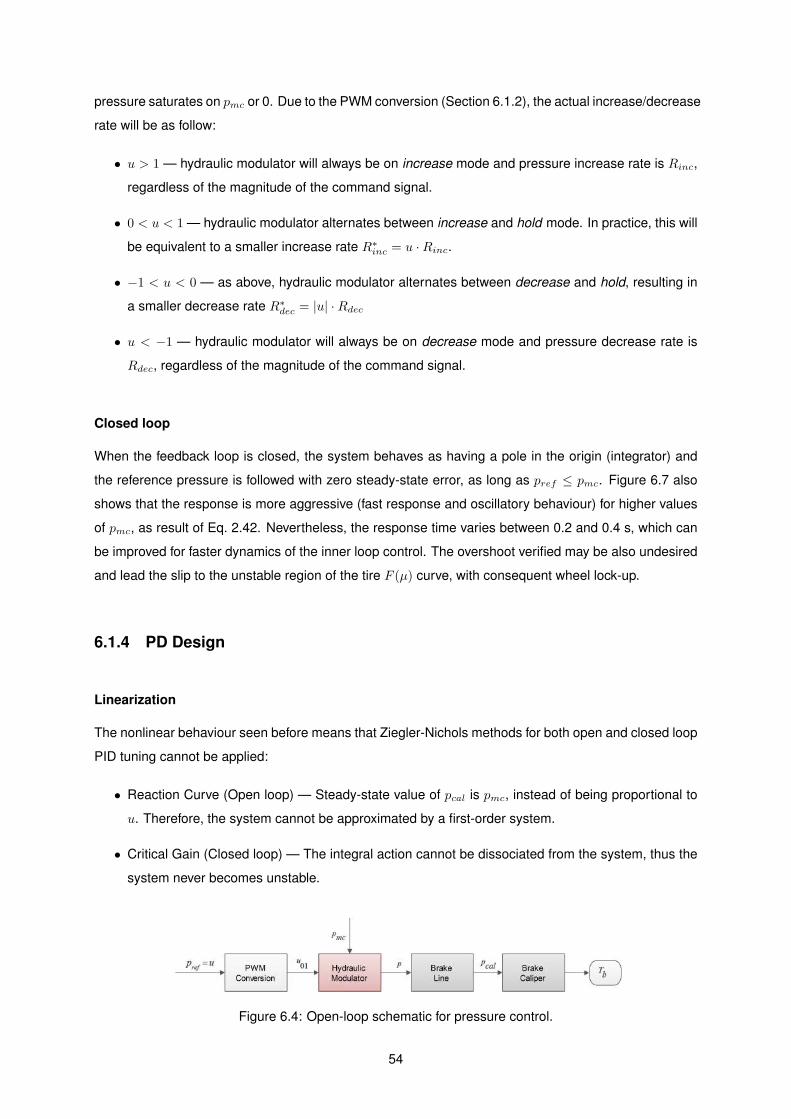
pressure saturates on pmc or 0. Due to the PWM conversion (Section 6.1.2), the actual increase/decrease
rate will be as follow:
• u > 1 — hydraulic modulator will always be on increase mode and pressure increase rate is Rinc,
regardless of the magnitude of the command signal.
• 0 < u < 1 — hydraulic modulator alternates between increase and hold mode. In practice, this will
be equivalent to a smaller increase rate R∗inc = u ·Rinc.
• −1 < u < 0 — as above, hydraulic modulator alternates between decrease and hold, resulting in
a smaller decrease rate R∗dec = |u| ·Rdec
• u < −1 — hydraulic modulator will always be on decrease mode and pressure decrease rate is
Rdec, regardless of the magnitude of the command signal.
Closed loop
When the feedback loop is closed, the system behaves as having a pole in the origin (integrator) and
the reference pressure is followed with zero steady-state error, as long as pref ≤ pmc. Figure 6.7 also
shows that the response is more aggressive (fast response and oscillatory behaviour) for higher values
of pmc, as result of Eq. 2.42. Nevertheless, the response time varies between 0.2 and 0.4 s, which can
be improved for faster dynamics of the inner loop control. The overshoot verified may be also undesired
and lead the slip to the unstable region of the tire F (µ) curve, with consequent wheel lock-up.
6.1.4 PD Design
Linearization
The nonlinear behaviour seen before means that Ziegler-Nichols methods for both open and closed loop
PID tuning cannot be applied:
• Reaction Curve (Open loop) — Steady-state value of pcal is pmc, instead of being proportional to
u. Therefore, the system cannot be approximated by a first-order system.
• Critical Gain (Closed loop) — The integral action cannot be dissociated from the system, thus the
system never becomes unstable.
Figure 6.4: Open-loop schematic for pressure control.
54

0 0.2 0.4 0.6 0.8 1 1.2 1.4 1.6 1.8 2 2.2 2.4−1
0
1
2
Time (s)
uin
0 0.2 0.4 0.6 0.8 1 1.2 1.4 1.6 1.8 2 2.2 2.4−5
0
5
10
Time (s)
Pre
ssur
e(M
Pa)
pref
pcal(pmc = 5)
pcal(pmc = 10)
0 0.2 0.4 0.6 0.8 1 1.2 1.4 1.6 1.8 2 2.2 2.4−1
0
1
2
Time (s)
uou
t
Figure 1.5: Open-loop variable-step response.
5
Figure 6.5: Open-loop variable-step response.
Figure 6.6: Closed-loop schematic for pressure control.
An alternative method is to approximate both PWM conversion and hydraulic modulator models by a
linearisable function that receives the command signal u and outputs the pressure p. Assuming pmc =
∞:
dpdt = Rinc for u ≥ 1
dpdt = u ·Rinc for 0 ≤ u < 1
dpdt = |u| ·Rdec for −1 < u < 0
dpdt = Rdec for u ≤ −1
' dp
dt= a · tanh(b · u+ h) + v (6.4)
55

0 0.2 0.4 0.6 0.8 1 1.2 1.4 1.6 1.8 2 2.2 2.4−1
0
1
2
Time (s)
uin
0 0.2 0.4 0.6 0.8 1 1.2 1.4 1.6 1.8 2 2.2 2.4
0
5
10
Time (s)
Pre
ssur
e(M
Pa)
pref
pcal(pmc = 5)
pcal(pmc = 10)
u (pmc = 5)
u (pmc = 10)
0 0.2 0.4 0.6 0.8 1 1.2 1.4 1.6 1.8 2 2.2 2.4−1
0
1
2
Time (s)
uou
t
Figure 1.7: Closed-loop variable-step response.
6
Figure 6.7: Closed-loop variable-step response.
The resulting linearisable function dpdt = f(u) is plotted in Fig. 6.8. The step response of the approx-
imated system (the transfer function on Eq. 2.41 is still used to model transient dynamics between p
and pcal) is depicted in Fig. 6.9. Although the approximation quality decays over time, it is qualitatively
accurate.
PD Tuning
Since the approximated system can now be linearised, Matlab’s PID Tuning tool can be used to automat-
ically calculate proportional and derivative gainsKP andKD, as well as the filter coefficientN , according
to the desired fastness and robustness of the step response (Eq. 6.5). Recalling the closed-loop step
response characteristics on Section 6.1.3 (no steady-state error), the integral gain is not included. After
calculating the values in Table 6.1 using the approximated system, the designed PID is used to control
the original system. Figure 6.10 displays the controlled step response of the original system and shows
that it was possible to eliminate the overshoot whilst maintaining a very fast response.
GPID = KP +KD ·N
1 +N 1s
(6.5)
56
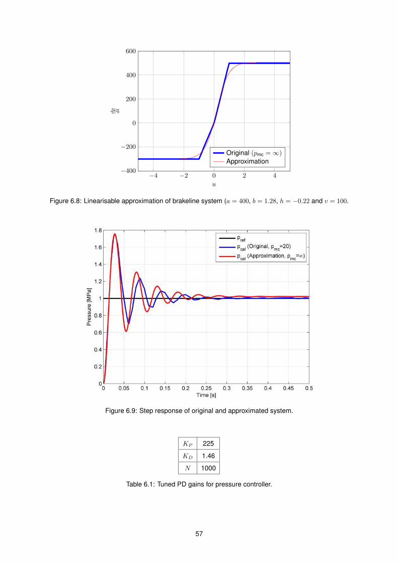
−4 −2 0 2 4−400
−200
0
200
400
600
u
dpdt
Original (pmc =∞)
Approximation
Figure 6.8: Linearisable approximation of brakeline system (a = 400, b = 1.28, h = −0.22 and v = 100.
Figure 6.9: Step response of original and approximated system.
KP 225
KD 1.46
N 1000
Table 6.1: Tuned PD gains for pressure controller.
57

0 5 · 10−2 0.1 0.15 0.2 0.25 0.3 0.35 0.4 0.45 0.50
0.2
0.4
0.6
0.8
1
1.2
1.4
1.6
1.8
2
Time (s)
Pre
ssur
e(M
Pa)
pref
pcal(Original)pcal(PID)
Figure 1.10: Step response with PD controller for pcal.
9
Figure 6.10: Step response with PD controller for pcal.
6.2 Wheel Slip Controller
Following the proposed approach in Chapter 5, the wheel slip controller is built upon a PID-type fuzzy
control structure, which combines the already introduced PID control principles with the fuzzy inference
system (FIS) theory.
For the wheel slip controller design, one will for now assume that the vehicle velocity v is directly
known from wheel and vehicle dynamic model.
6.2.1 FIS Overview
Fuzzy inference is the process of formulating the mapping from a given input to an output using fuzzy
logic. The basic structure of a fuzzy inference system consists of three conceptual components: a
rule base, which contains a selection of fuzzy if-then rules; a database, which defines the membership
functions used in the fuzzy rules; and a reasoning mechanism, which performs the inference procedure
upon the rules [15].
Takagi-Sugeno-Kang Fuzzy Inference System (FIS)
The proposed controller uses a Takagi-Sugeno-Kang (TSK) FIS is selected. The main difference be-
tween the more general Mamdani and TSK fuzzy models lie on the nature of the consequent, which are
respectively fuzzy set or a crisp value given by a constant or linear function of the inputs [33].
TSK fuzzy system rules r have the general form
58

Figure 6.11: Fuzzy inference system diagram.
Rr: If xi = Aj then yk = C0,k + C1,kx1 + . . .+ Cn,kxn
where xi is the input i = 1, . . . ,m, Aj is the fuzzy set j = 1, . . . , s, and yk is the output function k =
1, . . . , n, which a linear combination of the inputs.
The individual output yk of each rule is weighted by the firing strength wr of the rule, which is calcu-
lated using the min as the AND (T-norm operator):
Ruler : wr = mini{µi,Aj} for i = 1, . . . ,m and j = 1, . . . , s (6.6)
where µi,Aj is the fuzzy set Aj membership function value of input xi.
Hence, the procedures involved in the computation of the output signals are also distinct between
Mamdani and TSK fuzzy systems. In the former case the output is computed as a weighted average1 of
all rule outputs:
y =
∑ij wij .yij∑ij wij
(6.7)
6.2.2 FIS Design
Fuzzy sets
Has described in Section 5.2.2, the controller has two input variables eSX and ∆eSX . Three fuzzy sets
are defined for each input variable, according to Table 6.2. Similarly, five zero-order functions for the
output ∆prefb are defined, as listed in Table 6.3.
1The weighted sum (numerator of weighted average) is also an alternative method for output calculation with even more reducedcomputational effort
59

Fuzzy Set Classical Set c σ Description
A1 Negative eSX < 0 -1 0.425 SX is below reference slip, within thestable region of the tire friction curve(brake pressure too low)
A2 Zero eSX = 0 0 0.425 SX is equal to the desired referenceand FXT is maximum
A3 Positive eSX > 0 1 0.425 SX beyond reference slip, within theunstable region of the tire friction curve(brake pressure is too high)
B1 Decreasing ∆eSX < 0 -1 0.425 SX is increasing, thus evolving towardsor away from the reference value,whether SX is within the unstable orstable region, respectively
B2 Steady ∆eSX = 0 0 0.425 SX is not decreasing nor increasing
B3 Increasing ∆eSX > 0 1 0.425 SX is decreasing, thus evolving to-wards or away from the referencevalue, whether SX is within the stableor unstable region, respectively
Table 6.2: Fuzzy sets and MFs parameters for inputs eSX and ∆eSX .
yk Fuzzy Set Ck Description
1 Decrease-fast -1 Decrease reference pressure rapidly
2 Decrease-slow -0.5 Decrease reference pressure slowly
3 Hold 0 Hold reference pressure
4 Increase-slow 0.5 Increase reference pressure slowly
5 Increase-fast 1 Increase reference pressure rapidly
Table 6.3: TSK consequent function parameters for output ∆prefb .
Membership Functions
Membership functions (MFs) for the input variables are similar and defined by Gaussian curves (Eq. 6.8)
whose parameters are the variance σ and center of gravity c.
µi,Ai = µi,Bj = Gaussian(x; c, σ) = e−(x−c)2
2σ2 (6.8)
The choice of Gaussian curves over, e.g. triangular or trapezoidal MFs, ensures a smoother transition
between fuzzy sets, which translates into a continuous output signal. MFs for each fuzzy set, as depicted
by Fig. 6.12, are evenly distributed within the normalized interval [−1 1] (universe of discourse). Doing
so ensures that the controller dynamics are easily adjusted solely by tuning the PID gains outside the
FIS. The parameters for all input MFs are listed in Table 6.2.
Rule Set
For this specific problem, a set of rules is established as follow:
60

Figure 6.12: Membership functions of FIS.
Rr: If eSX is Ai and ∆eSX is Bj then ∆prefb is Ck
where the indexes i and j refer to a possible combination in Table 6.4.
HHHHHAi
Bj Decreasing Steady Increasing
Negative Increase-fast Increase-slow Hold
Zero Increase-slow Hold Decrease-slow
Positive Hold Decrease-slow Decrease-fast
Table 6.4: Fuzzy rules for wheel slip controller.
Output surface
The FIS output surface is displayed in Fig. 6.13. In general, the reference pressure variation ∆prefb is
more or less inversely proportional to the inputs, as in a PD controller. Slight variations of this linear
relation, shown by the humps and valleys on the surface plot, ensure the adaptation of the controller
on whether the system is evolving near/far from the reference slip or within/towards the stable/unstable
region of the friction curve.
61

Figure 6.13: Output surfaces of FIS models for wheel slip controller.
6.2.3 PID Gains Optimization
The input and output gains Ke, K∆e where firstly tuned so the signal values entering the FIS would
range within the normalized interval [−1 1]. As for the output gain K∆p, the value for the first iteration
was chosen according to the actuator limits of pressure increase/decrease rate (Table 7.2). The three
parameters where then optimized, as to minimize the MSE to the reference SrefX signal. Optimization is
performed using the Simulink Design Optimization tool, with the default method Gradient descent and
algorithm Sequential Quadratic Programming. The final values are listed in table Table 6.5
Ke 1.92
K∆e 0.08
K∆p 1159
Table 6.5: Tuned PID gains for fuzzy wheel slip controller.
6.2.4 Reference Wheel Slip
The reference wheel slip that is fed to the newly designed controller is the last decision variable. From
the tire friction model curves displayed in Chapter 3, tire braking force magnitude (FXT < 0 is maximized
near SX = −0.2. After some iterations during the simulation phase, the reference wheel slip SrefX is fixed
in
SrefX = −0.16 (6.9)
62
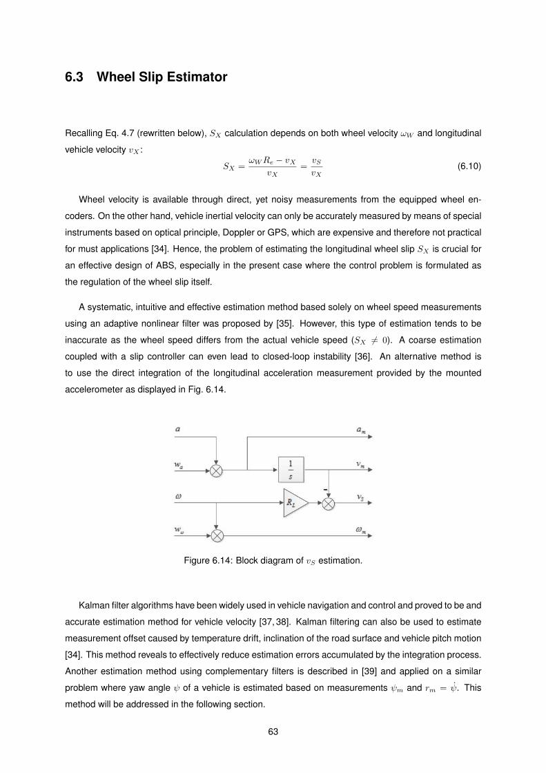
6.3 Wheel Slip Estimator
Recalling Eq. 4.7 (rewritten below), SX calculation depends on both wheel velocity ωW and longitudinal
vehicle velocity vX :
SX =ωWRe − vX
vX=vSvX
(6.10)
Wheel velocity is available through direct, yet noisy measurements from the equipped wheel en-
coders. On the other hand, vehicle inertial velocity can only be accurately measured by means of special
instruments based on optical principle, Doppler or GPS, which are expensive and therefore not practical
for must applications [34]. Hence, the problem of estimating the longitudinal wheel slip SX is crucial for
an effective design of ABS, especially in the present case where the control problem is formulated as
the regulation of the wheel slip itself.
A systematic, intuitive and effective estimation method based solely on wheel speed measurements
using an adaptive nonlinear filter was proposed by [35]. However, this type of estimation tends to be
inaccurate as the wheel speed differs from the actual vehicle speed (SX 6= 0). A coarse estimation
coupled with a slip controller can even lead to closed-loop instability [36]. An alternative method is
to use the direct integration of the longitudinal acceleration measurement provided by the mounted
accelerometer as displayed in Fig. 6.14.
Figure 6.14: Block diagram of vS estimation.
Kalman filter algorithms have been widely used in vehicle navigation and control and proved to be and
accurate estimation method for vehicle velocity [37, 38]. Kalman filtering can also be used to estimate
measurement offset caused by temperature drift, inclination of the road surface and vehicle pitch motion
[34]. This method reveals to effectively reduce estimation errors accumulated by the integration process.
Another estimation method using complementary filters is described in [39] and applied on a similar
problem where yaw angle ψ of a vehicle is estimated based on measurements ψm and rm = ψ. This
method will be addressed in the following section.
63

6.3.1 Complementary Filter
A complementary filter, i.e., a Wiener filter equivalent to the stationary Kalman filter solution, arise nat-
urally in the context of signal estimation based on measurements provided by sensors over distinct, yet
complementary regions of frequency. For the specific problem of slip velocity estimation, complemen-
tary filter combines low frequency information from accelerometer with high frequency measurements
from wheel speed encoders. The relative amount of information from each sensor is adjusted through
the Kalman gain K.
ˆvS = K (ωmRe − (vS + vm)) (6.11)
where
ωW,m ≡ ωm = ωW + wω (6.12)
vX,m ≡ vm = ∫(aX + wa) (6.13)
Figure 6.15: Block diagram of complementary filter.
The estimate longitudinal slip ratio is then calculated by dividing the newly estimated slip velocity vS
by the
SX =vS∫ am
(6.14)
64
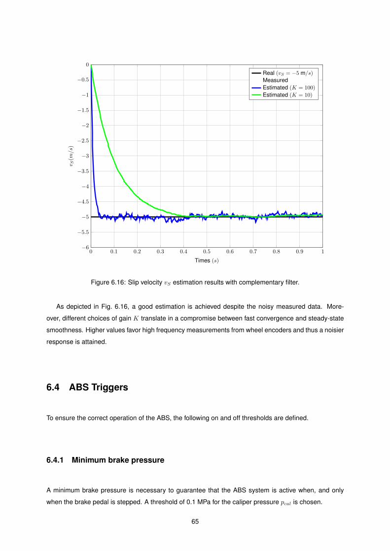
0 0.1 0.2 0.3 0.4 0.5 0.6 0.7 0.8 0.9 1−6
−5.5
−5
−4.5
−4
−3.5
−3
−2.5
−2
−1.5
−1
−0.5
0
Times (s)
v S(m/s
)Real (vS = −5 m/s)MeasuredEstimated (K = 100)
Estimated (K = 10)
Figure 1.16: Slip velocity vS estimation results with complementary filter.
16
Figure 6.16: Slip velocity vS estimation results with complementary filter.
As depicted in Fig. 6.16, a good estimation is achieved despite the noisy measured data. More-
over, different choices of gain K translate in a compromise between fast convergence and steady-state
smoothness. Higher values favor high frequency measurements from wheel encoders and thus a noisier
response is attained.
6.4 ABS Triggers
To ensure the correct operation of the ABS, the following on and off thresholds are defined.
6.4.1 Minimum brake pressure
A minimum brake pressure is necessary to guarantee that the ABS system is active when, and only
when the brake pedal is stepped. A threshold of 0.1 MPa for the caliper pressure pcal is chosen.
65

6.4.2 Wheel slip and wheel slip rate trigger
The combined information of wheel slip and wheel slip rate provide an indication on whether or not the
wheel may lock. If wheel slip is beyond reference slip (unstable region) or decreasing at a high rate
(towards lock-up), ABS should start its action. Recalling Table 6.4, these conditions correspond also to
the rules where the pressure should be decreased, initiating the control cycle. Trigger values are defined
as SX = −0.1 and ∆SX = −2.
6.4.3 Low velocity trigger
Rewriting Eq. 4.7 in the form
SX =ωW .RL − vX
vX⇔ ωW =
vX(1 + SX)
RL(6.15)
and assuming that a constant wheel slip, i.e. dSXdt = 0, as the vehicle tends to complete stoppage, both
vehicle velocity and wheel velocity tend, naturally, to zero.
limvX→0
ωW = 0 (6.16)
In practice, this means that the SX calculation/estimation will tend to a zero-by-zero division and may
become unstable.
limvX→0
SX =0− 0
0(6.17)
Since FS prototypes rarely run slow enough so this problem may occur, a vehicle velocity threshold of
20 km/h (5.6 m/s) was enforced, below which the ABS controller is turned off. Increasingly bigger os-
cillations around the reference wheel slip are thus avoided, which exceedingly degraded ABS efficiency
and could even drive the system towards instability.
66

Chapter 7
Simulation Results and Analysis
This chapter contains the final simulation results. Firstly, simulation parameters are listed (Section 7.1).
Then, a set of braking simulations are performed are compared between a vehicle with and without the
design controller, including the wheel slip estimation and sensor noise, for a constant µ (Section 7.2.1)
and real-time varying (Section 7.2.2) road type. The role of the inner brake pressure controller on the
ABS performance is also tested (Section 7.2.3). Finally, a complete lap around a typical Autocross circuit
provides the information on the real advantage of a ABS-equipped FS prototype (Section 7.3).
7.1 Simulation Parameters
7.1.1 FST 05e Parameters
The most relevant data needed for modelling and simulation purposes are available via CAD tools or
physical measurements. The complete set parameters’ values for the FST 05e is listed in Table 7.1.
Other model and simulation parameters are listed in Table 7.2.
7.2 Straight Line Hard Braking
The first set of simulations to be performed are simple hard braking manoeuvres: initially the vehicle
travels at constant velocity vX = v0; at t = 1 s, the driver steps hard on the pedal brake (so that
Tb � FXT .RL) and keeps it until the vehicle stops. The term acceleration refers to the magnitude of the
acceleration henceforth.
67
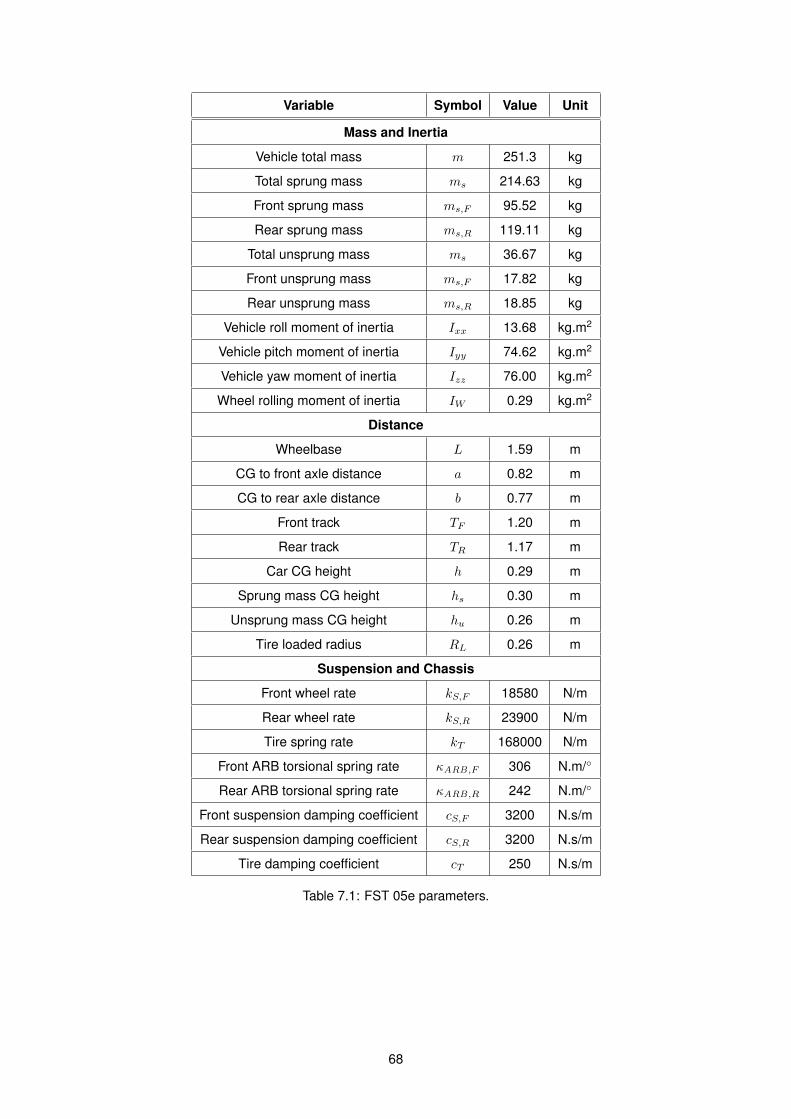
Variable Symbol Value Unit
Mass and Inertia
Vehicle total mass m 251.3 kg
Total sprung mass ms 214.63 kg
Front sprung mass ms,F 95.52 kg
Rear sprung mass ms,R 119.11 kg
Total unsprung mass ms 36.67 kg
Front unsprung mass ms,F 17.82 kg
Rear unsprung mass ms,R 18.85 kg
Vehicle roll moment of inertia Ixx 13.68 kg.m2
Vehicle pitch moment of inertia Iyy 74.62 kg.m2
Vehicle yaw moment of inertia Izz 76.00 kg.m2
Wheel rolling moment of inertia IW 0.29 kg.m2
Distance
Wheelbase L 1.59 m
CG to front axle distance a 0.82 m
CG to rear axle distance b 0.77 m
Front track TF 1.20 m
Rear track TR 1.17 m
Car CG height h 0.29 m
Sprung mass CG height hs 0.30 m
Unsprung mass CG height hu 0.26 m
Tire loaded radius RL 0.26 m
Suspension and Chassis
Front wheel rate kS,F 18580 N/m
Rear wheel rate kS,R 23900 N/m
Tire spring rate kT 168000 N/m
Front ARB torsional spring rate κARB,F 306 N.m/◦
Rear ARB torsional spring rate κARB,R 242 N.m/◦
Front suspension damping coefficient cS,F 3200 N.s/m
Rear suspension damping coefficient cS,R 3200 N.s/m
Tire damping coefficient cT 250 N.s/m
Table 7.1: FST 05e parameters.
68

Variable Symbol Value Unit
Initial vehicle velocity v0 100 km/h
Pedal force Fbp 600 N
PWM modulator signal frequency fc 100 Hz
Pressure increase rate Rinc 800 MPa/s
Pressure decrease rate Rdec 500 MPa/s
Hydraulic lag τ 0.02 s
Sample time Ts 0.002 s
Table 7.2: Other model and simulation parameters.
7.2.1 Constant µ
A constant value for the road coefficient of friction is firstly tested, with µ = 0.80 (dry road). Figure 7.1
plots over time the comparative simulation results with (solid line) and without (dashed line) the designed
ABS scheme. Plots depict, from top to bottom, vehicle position (xE), vehicle and wheel velocities (vX
and ωW ), followed by the vehicle longitudinal acceleration (aX ), the wheel slip (SX ) and its reference
value, and the pressures on the master cylinder (pmc), wheel caliper (pcal) and reference prefb . The
simulation case without ABS serves both as validation for the vehicle and tire dynamic models and a
term of comparison for further simulations with the designed ABS.
Up to t = 1 s, wheel tangential velocity ω.RL equals the vehicle velocity for both cases, i.e., wheel is
in free-rolling condition (SX = 0). When the driver starts braking without ABS, wheel rapidly decelerates,
until it locks-up. This is also shown by the value of SX heading towards -1. If the vehicle is equipped
with the ABS, wheel velocity decreases as fast, until the reference slip SrefX = −0.16 is matched and
efficiently tracked.
Regarding the aX plot, it is noticeable that, for both cases, a maximum acceleration of |aX | ' 30 m/s2
is soon reached. As expected, this occurs when SX = SrefX , i.e., when SX crosses the optimal value for
which peak longitudinal force is attained, as shown in Fig. 4.3 and described in Section 4.3.2. However,
the ABS is able to keep maximum acceleration thenceforth, thus resulting in a steeper velocity plot, and
a smaller braking time and distance. Final numeric results are listed on Table 7.3.
Observing the pressure plot for a braking without ABS, pressure on the caliper quickly matches
the pressure on the master cylinder (a certain dynamic can be noticed). On the other hand, the ABS
managed to initially increase pressure near the maximum rate allowed by the actuator, i.e., similar to the
case without ABS. The increase rate is then slowed to avoid overshot when the wheel slip approaches
the reference value.
69

0 0.2 0.4 0.6 0.8 1 1.2 1.4 1.6 1.8 2 2.2 2.40
10
20
30
Velo
city
(m/s) ω.RL
vX
0 0.2 0.4 0.6 0.8 1 1.2 1.4 1.6 1.8 2 2.2 2.40
10
20
30
40
xE
(m/s
)
0 0.2 0.4 0.6 0.8 1 1.2 1.4 1.6 1.8 2 2.2 2.4−40
−20
0
20
aX
(m2/s)
0 0.2 0.4 0.6 0.8 1 1.2 1.4 1.6 1.8 2 2.2 2.4−1
−0.8
−0.6
−0.4
−0.20
SX
SrefX
SX
0 0.2 0.4 0.6 0.8 1 1.2 1.4 1.6 1.8 2 2.2 2.40
5
10
15
20
Time (s)
pca
l(M
Pa) pref
pmcpcal
Figure 1.1: Comparative simulation results with (solid) and without (dashed) ABS.
4
Figure 7.1: Comparative simulation results with (solid) and without (dashed) ABS.
Without ABS With ABS ∆ %∆
Braking Distance (m) 21.87 15.21 -6.66 -30.5 %
Braking Time (s) 1.63 1.17 -0.46 -28.2 %
Table 7.3: Braking distance and time results with and without ABS.
70

7.2.2 Varying µ
0 0.2 0.4 0.6 0.8 1 1.2 1.4 1.6 1.8 2−40
−20
0
20
aX
(m2/s
)
0 0.2 0.4 0.6 0.8 1 1.2 1.4 1.6 1.8 20
10
20
30
Velo
city
(m/s)
ω.RLvX
0 0.2 0.4 0.6 0.8 1 1.2 1.4 1.6 1.8 2−1
−0.8
−0.6
−0.4
−0.2
0
SX
(−)
SrefX
SX
0 0.2 0.4 0.6 0.8 1 1.2 1.4 1.6 1.8 20
5
10
15
20
Time (s)
pca
l(M
Pa)
pref
pmcpcal
Figure 1.2: Simulation results with varying µ.
5
Figure 7.2: Simulation results with varying µ.
To test the adaptivity of the proposed ABS controller to real-time variations of the surface type, the
following values for the road coefficient of friction µ have been introduced as input parameter on the
Pacejka tire model (Section 3.1.1):
µ = 0.8 for t < 0.75s
µ = 0.5 for 0.75 ≤ t < 1.25s
µ = 0.8 for t ≥ 1.25s
(7.1)
The resulting plots on Fig. 7.2 evidence a fast adaptation of the controller with varying coefficient
of friction. At t = 0.75 s, µ suddenly decreases, which also decreases the available tire force that is
reacting the brake torque. Consequently, wheel slip enters the unstable region of tire friction curve and
71

decays abruptly towards lock-up. Since pressure must be released to counter-act this effect, the slip
controller immediately diminishes the reference pressure. After a brief undershot, reference pressure
stabilizes near 5 MPa in about 0.1 s and wheel slip is restored to the reference slip value. At t = 1.25
s, the opposite phenomenon occurs and brake pressure can again be increased to maximize tire force.
Since wheel slip is now within the stable region, the reference pressure is increased slower and tracked
without overshoot, with wheel slip settling in 0.2 s.
7.2.3 Without pressure controller
To simulate the ABS system without the inner loop, the reference pressure variance ∆prefb is directly feed
into the hydraulic modulator as the command signal u, as depicted in Fig. 7.3. Figure 7.4 evidences that
the pressure PID controller plays a major role on ABS performance. Even though wheel slip controller
gains are not optimized, since it cannot cope with the hydraulic lag dynamics simulation results show
continuous oscillation of the wheel slip around the reference value instead of settling.
Figure 7.3: Control scheme without pressure inner loop.
With PD Without PD ∆ %∆
Braking Distance (m) 15.21 16.14 +0.93 +6.11 %
Braking Time (s) 1.17 1.28 +0.11 +9.40 %
Table 7.4: Braking distance and time without PD pressure controller.
7.3 Complete Lap
The absolute advantage of the ABS on a FS prototype is more evident on a complete Autocross1 lap is
simulated with modified GG diagrams for the case with and without ABS. The GG diagram is a plot used
to describe the performance of a car, since it contains the envelope of the combinations of longitudinal
(driving and braking) and lateral accelerations attainable by the tires, in units of g = 9.8 m/s2. As
described in chapters 3 and 4, the absence of an ABS may lead to wheel lock, i.e. SX = −1, for which1The Autocross Event consists of a timed lap around a tight course to evaluate the car’s maneuverability and handling qualities,
combining the performance features of acceleration, braking, and cornering.
72
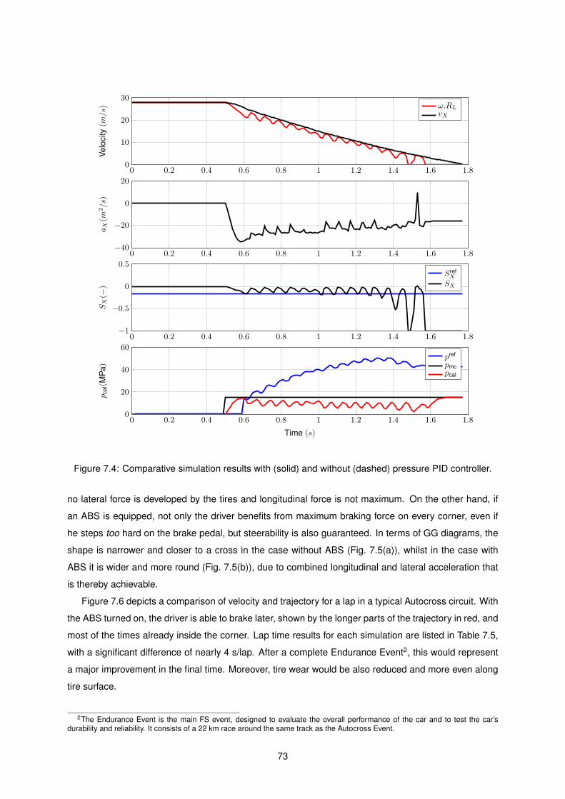
0 0.2 0.4 0.6 0.8 1 1.2 1.4 1.6 1.8−40
−20
0
20
aX
(m2/s)
0 0.2 0.4 0.6 0.8 1 1.2 1.4 1.6 1.80
10
20
30Ve
loci
ty(m/s)
ω.RLvX
0 0.2 0.4 0.6 0.8 1 1.2 1.4 1.6 1.8−1
−0.5
0
0.5
SX
(−)
SrefX
SX
0 0.2 0.4 0.6 0.8 1 1.2 1.4 1.6 1.80
20
40
60
Time (s)
pca
l(M
Pa)
pref
pmcpcal
Figure 1.4: Comparative simulation results with (solid) and without (dashed) pressure PID controller.
7
Figure 7.4: Comparative simulation results with (solid) and without (dashed) pressure PID controller.
no lateral force is developed by the tires and longitudinal force is not maximum. On the other hand, if
an ABS is equipped, not only the driver benefits from maximum braking force on every corner, even if
he steps too hard on the brake pedal, but steerability is also guaranteed. In terms of GG diagrams, the
shape is narrower and closer to a cross in the case without ABS (Fig. 7.5(a)), whilst in the case with
ABS it is wider and more round (Fig. 7.5(b)), due to combined longitudinal and lateral acceleration that
is thereby achievable.
Figure 7.6 depicts a comparison of velocity and trajectory for a lap in a typical Autocross circuit. With
the ABS turned on, the driver is able to brake later, shown by the longer parts of the trajectory in red, and
most of the times already inside the corner. Lap time results for each simulation are listed in Table 7.5,
with a significant difference of nearly 4 s/lap. After a complete Endurance Event2, this would represent
a major improvement in the final time. Moreover, tire wear would be also reduced and more even along
tire surface.
2The Endurance Event is the main FS event, designed to evaluate the overall performance of the car and to test the car’sdurability and reliability. It consists of a 22 km race around the same track as the Autocross Event.
73
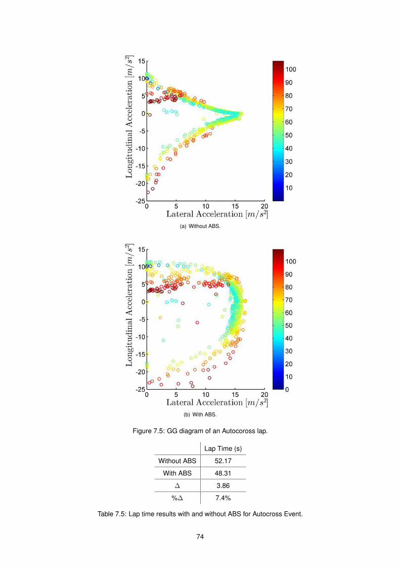
(a) Without ABS.
(b) With ABS.
Figure 7.5: GG diagram of an Autocoross lap.
Lap Time (s)
Without ABS 52.17
With ABS 48.31
∆ 3.86
%∆ 7.4%
Table 7.5: Lap time results with and without ABS for Autocross Event.
74
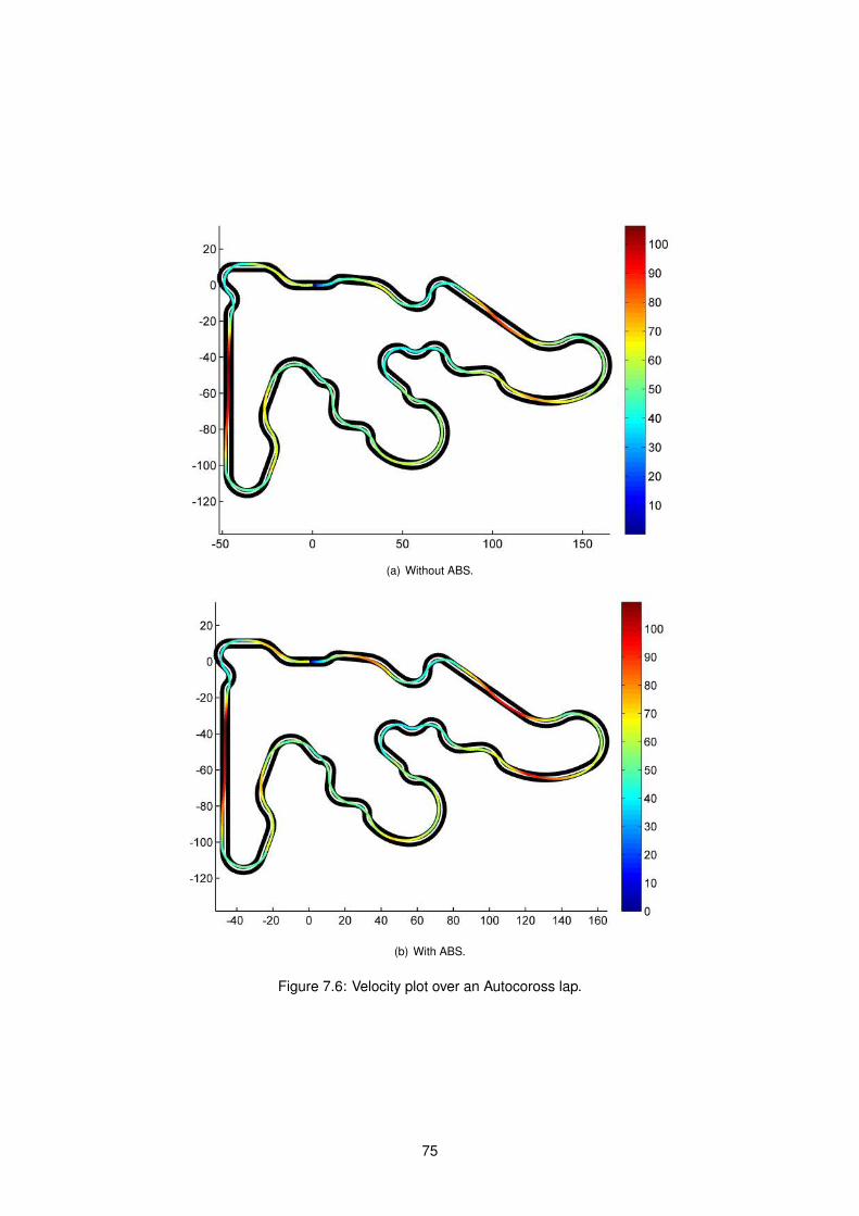
(a) Without ABS.
(b) With ABS.
Figure 7.6: Velocity plot over an Autocoross lap.
75
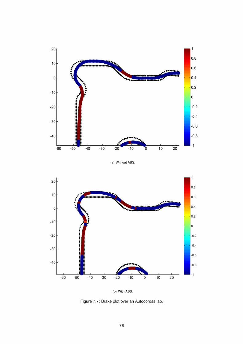
(a) Without ABS.
(b) With ABS.
Figure 7.7: Brake plot over an Autocoross lap.
76

Chapter 8
Summary and Conclusions
This thesis reported the design of an ABS application for a Formula Student (FS) prototype, with the
objectives of reducing braking distance while ensure steering stability. For this purpose, a cascade
control architecture containing two feedback loops was proposed for enhanced performance. The outer
loop and main controller makes use of a PID-type fuzzy system for wheel slip regulation, allying the well-
known control PID theory with the intuitive design and computational efficiency of a FIS, whilst the inner
loop resorted to a conventional and easily implementable PD controller for brake pressure reference
tracking.
For the ABS design process and further simulation, a self-developed vehicle model with 14 DOFs
was built upon the principles of vehicle dynamics, mainly under braking (Chapter 2). The full model was
divided into the following sub-models: horizontal model for the position (xE and yE) and orientation (yaw
angle ψ) of the vehicle’s CG in the inertial reference plane, as it is subjected to tire forces and moments;
a 7-DOFs vibrational model of the vehicles submitted to aerodynamic and load transfer loads, which
allowed the real-time computation of transient tire vertical loads, as well as the vertical displacements
of the sprung zs and unsprung masses zu,i), roll angle φ and pitch angle θ; wheel dynamics, for wheel
kinematics (ωWandωW ) as result of an applied brake torque and the tire longitudinal force; brakeline
dynamics, namely the hydraulic lag phenomenon and a transient model of the hydraulic modulator.
An accurate tire friction model is of absolute importance for ABS applications. With that in mind,
special attention has been given to this subject in Chapter 3. Taking advantage of reliable experimental
data from a renowned tire test facility, three types of tire models were designed and compared: the
well-known and widely used Pacejka’s Magic Formula (MF), the Burkhardt velocity-dependant model,
and an self-developed new approach using artificial neural network (ANN). Fitting results showed that
Pacejka was the most suitable tire model, providing accurate longitudinal tire force FXT mapping for
a wider range of possible SX , including the wheel lock-up case SX = −1. The accurateness of the
other two models was compromised for extrapolation beyond the limits of experimental data availability.
Later simulation results allowed the validation of the complete vehicle and tire model integration, namely
vehicle and wheel kinematics throughout braking.
The ABS problem was then introduced from the control theory point of view: the object variable SX ,
77

mathematically defined as the longitudinal (wheel) slip ratio should be kept within a range for which
longitudinal and lateral tire forces are near its peak values (Chapter 4). Some of the the most common
and relevant solutions were then reviewed, namely threshold control, PID control, sliding-mode control
(SMC) and the emerging new approaches on intelligent control. Threshold control applies a basic, yet
widely used control algorithm, mainly in the early versions of the ABS. Since the control algorithm is
solely based on binary relations between input variables and threshold values, this method is nowadays
a limited solution and lacks some of the controllability and efficiency of other control methods. PID
control is a very versatile and well-known control method for numerous applications. Its hybridization
with other control techniques provided the necessary robustness, self-tuning or adaptability features
for ABS employment, which naturally enhanced the already satisfactory controller performance. SMC
is a more complex but particularly effective method for ABS control, given the robustness properties
and applicability to nonlinear plants. Published results on this subject exhibit excellent performance
for a wide variety of conditions and reinforced the suitableness of SMC for wheel slip manipulation.
Finally, a research has been put through on the later intelligent control solutions for the ABS problem.
Though diversity of resources and applications is, in fact, very broad and arbitrary complex, a few notable
publications were considered and revised, namely on the areas of fuzzy or neuro-fuzzy theory and
genetic algorithm (GA) optimization.
Considering the characteristics of the reviewed methods, as well as the available information on the
ABS target vehicle and the FS competition requirements, the aforementioned proposal is introduced
(Chapter 5). Then, the ABS design was streamlined into the following components: brake pressure
controller, wheel slip controller, and wheel slip estimator (Chapter 6).
Due to the dynamic characteristics of the inner loop plant, i.e., brakeline and hydraulic modulator
system, the regular Ziegler–Nichols methods for open and closed loop could not be applied. Therefore,
a linearisable approximate model of the plant was arranged, so that Matlab’s PID Tuning tool could be
used. PD gains were tuned in order to achieve the desired fast dynamics, near the actuator limit, without
overshoot, which could let the wheel slip to the unstable region of the tire friction curve. As for the
PID-type fuzzy controller, a Takagi-Sugeno-Kang (TSK) fuzzy inference system (FIS) was selected and
modelled with two inputs variables for the slip error eSX and its time-step variance ∆eSX . A rule set for
the output reference pressure variance ∆prefb was selected based on conventional ABS increase-hold-
decrease cycles. The external PID gains were then iteratively tuned for optimal controller performance,
i.e., braking distance minimization with reduced tracking oscillations.
In what concerns wheel slip estimation, a solution using a complementary filter was implemented,
i.e., a Wiener filter equivalent to the stationary Kalman filter solution. Test results with noisy measure-
ments of the acceleration and wheel speed confirmed the efficiency of the filter on reducing signal noise
while ensuring good estimation accuracy. Moreover, this approach is simpler than the stochastic setting
proposed by Kalman, which requires a complete characterization of process and observation noises.
A set of hard braking simulations followed the design phase. Results shown in Chapter 7 and sum-
marized in Table 8.1 evidence a significant reduction of the braking time and distance. Furthermore,
the proposed controller exhibit a fast response and relatively smooth tracking of the reference wheel
78

slip. The robustness of the controller against sudden variations of the road coefficient of friction µ, both
high-to-low and low-to-high, was also successfully demonstrated. Further simulations without the in-
ner pressure manipulation testify the relevance of the PID controller on achieving the aforementioned
performance, namely by independently dealing with the hydraulic dynamics. A final simulation within a
complete lap around an typical Autocross circuit conclusively confirmed the competitive advantage of an
ABS-equipped FS prototype, by deducting nearly 4 seconds to the final lap.
8.1 Future work and research
As stated in the thesis’s objectives in Section 1.3, physical implementation of the proposed controller
was a concern. Having that mind during the modelling and design phases, special attention has already
been given to some important practical issues: sampling time, PWM conversion and noise filtering were
all considered. For that reason, hardware-in-the-loop validations and hardware implementations on a
real FS prototype are the natural steps to follow.
Besides that, further research on the following topics is recommended:
• Although the braking distance reduction and steerability objectives were already acomplished,
the stability of the vehicle on a asymmetric µ surface is not ensured (Section 4.1). A balancing
algorithm should then be implemented so that even tire forces on the right and left side of the car
are always a priority.
• As a electric vehicle, FST 05e makes use of an electric motor to drive each of the rear wheels,
which may introduce important inertial effects during braking that were not studied. Moreover, an
electric motor has the ease and flexibility to implement any control algorithm that may work closely
or instead the proposed ABS controller [40] and increase braking performance and/or stability.
• Oscillations around the reference wheel slip, mainly during the transient period, correspond to
oscillations in the acceleration of the car’s CG, which in turn are transmitted to the suspension
due to weight transfer. A comparative study between the frequency of these oscillations and the
natural frequency of the car’s suspension may be carried out using the vibrational model described
in Section 2.3. Results may be evaluated either in terms of the driver comfort or ABS enhancement
with an active suspension system, as proposed in [30].
Without ABS With ABS ∆ %∆
Braking Distance (m) 38.27 35.01 -3.26 -8.5 %
Braking Time (s) 3.52 3.25 -0.27 -7.7 %
Lap Time (s) 52.17 48.31 3.86 7.4%
Table 8.1: Results summary with and without ABS.
79

80

Bibliography
[1] MATLAB R2014a Documentation Center, MathWorks, 2014. [Online]. Available: http:
//www.mathworks.com/help/matlab/
[2] R. N. Jazar, Vehicle Dynamics: Theory and Application. Springer, 2008.
[3] A. Mirzaei, M. Moallem, B. Dehkordi, and B. Fahimi, “Design of an optimal fuzzy controller for
antilock braking systems,” IEEE Transactions on Vehicular Technology, vol. 55, no. 6, pp. 1725–
1730, Nov 2006.
[4] E. M. Kasprzak, “Capabilities report,” Calspan TIRF, Tech. Rep., 2012.
[5] Bosch Automotive Handbook, Electronic ed., Robert Bosch GmbH, 2002.
[6] C.-K. Chen and M.-C. Shih, “PID-Type Fuzzy Control for Anti-Lock Brake Systems with Parameter
Adaptation,” JSME International Journal Series C, vol. 47, pp. 675–685, 2004.
[7] “Vehicle dynamics terminology,” SAE Std. J670-2008, 2008.
[8] M. Brosnan, A. Sweat, J. Wood, and A. Radlbeck, “Anti-lock braking systems,” University of Con-
necticut, Tech. Rep., 2012.
[9] A. A. Aly, E.-S. Zeidan, A. Hamed, and F. Salem, “An antilock-braking systems (ABS) control: A
technical review,” Intelligent Control and Automation, no. 2, pp. 186–195, 2011.
[10] “Non-skid braking,” Flight Internacional, pp. 587–588, October 1953.
[11] R. Limpert, Brake Design and Safety, 2nd ed. SAE - Society of Automotive Engeneers, Inc., 1999.
[12] H. Raza, Z. Xu, B. Yang, and P. Ioannou, “Modeling and control design for a computer-controlled
brake system,” IEEE Transactions on Control Systems Technology, vol. 5, no. 3, pp. 279–296, May
1997.
[13] H. B. Pacejka, Tyre and Vehicle Dynamics, 3rd ed. Butterworth-Heinemann, 2012, ch. 4.
[14] C. C. de Wit, P. Tsiotras, E. Velenis, M. Basset, and G. Gissinger, “Dynamic friction models for
road/tire longitudinal interaction,” Vehicle System Dynamics, vol. 39, no. 3, pp. 189–226, 2003.
[15] J. S. R. Jang, C. T. Sun, and E. Mizutani, Neuro-Fuzzy and Soft Computing: A Computational
Approach to Learning and Machine lntelligence, 1st ed. Prentice-Hall, Inc., 1997, ch. 4.
81
[16] A. Harifi, A. Aghagolzadeh, G. Alizadeh, and M. Sadeghi, “Designing a sliding mode controller for
antilock brake system,” in The International Conference on Computer as a Tool (EUROCON), vol. 1,
Nov 2005, pp. 258–261.
[17] E. Velenis, P. Tsiotras, C. Canudas De Wit, and M. Sorine, “Dynamic Tire Friction Models for Com-
bined Longitudinal and Lateral Vehicle Motion,” Vehicle System Dynamics, vol. 43, no. 1, pp. 3–29,
2005.
[18] K. Z. Rangelov, “Simulink model of a quarter-vehicle with an anti-lock braking system,” Master’s
thesis, Eindhoven University of Technology, March 2004.
[19] C. Jun, “The study of ABS control system with different control methods,” in Proceedings of the 4th
International Symposium on Advanced Vehicle Control, 1998, pp. 623–628.
[20] T. K. Bera, K. Bhattacharya, and A. K. Samantaray, “Evaluation of antilock braking system with
an integrated model of full vehicle system dynamics,” Simulation Modelling Practice and Theory,
vol. 19, no. 10, pp. 2131–2150, November 2011.
[21] Q. Fu, L. Zhao, M. Cai, M. Cheng, and X. Sun, “Simulation research for quarter vehicle ABS on
complex surface based on PID control,” in 2nd International Conference on Consumer Electronics,
Communications and Networks (CECNet), April 2012, pp. 2072–2075.
[22] F. Jiang and Z. Gao, “An application of nonlinear PID control to a class of truck ABS problems,” in
Proceedings of the 40th IEEE Conference on Decision and Control, vol. 1, 2001, pp. 516–521 vol.1.
[23] E. Kayacan, Y. Oniz, and O. Kaynak, “A grey system modeling approach for sliding-mode control of
antilock braking system,” IEEE Transactions on Industrial Electronics, vol. 56, no. 8, pp. 3244–3252,
Aug 2009.
[24] J.-J. E. Slotine and W. Li, Applied Nonlinear Control. Prentice Hall, 1991, ch. 7.
[25] T. Shim, S. Chang, and S. Lee, “Investigation of sliding-surface design on the performance of sliding
mode controller in antilock braking systems,” IEEE Transactions on Vehicular Technology, vol. 57,
no. 2, pp. 747–759, March 2008.
[26] N. Patra and K. Datta, “Sliding mode controller for wheel-slip control of anti-lock braking system,” in
IEEE International Conference on Advanced Communication Control and Computing Technologies
(ICACCCT), Aug 2012, pp. 385–391.
[27] Y. Tang, X. Zhang, D. Zhang, G. Zhao, and X. Guan, “Fractional order sliding mode controller design
for antilock braking systems,” Neurocomputing, vol. 111, no. 0, pp. 122 – 130, 2013.
[28] A. V. Topalov, Y. Oniz, E. Kayacan, and O. Kaynak, “Neuro-fuzzy control of antilock braking system
using sliding mode incremental learning algorithm,” Neurocomputing, vol. 74, no. 11, pp. 1883 –
1893, 2011.
82
[29] N. Raesian, N. Khajehpour, and M. Yaghoobi, “A new approach in anti-lock braking system (ABS)
based on adaptive neuro-fuzzy self-tuning PID controller,” in 2nd International Conference on Con-
trol, Instrumentation and Automation (ICCIA), Dec 2011, pp. 530–535.
[30] W.-Y. Wang, M.-C. Chen, and S.-F. Su, “Hierarchical fuzzy-neural control of anti-lock braking system
and active suspension in a vehicle,” Automatica, vol. 48, no. 8, pp. 1698 – 1706, 2012.
[31] A. B. Sharkawy, “Genetic fuzzy self-tuning PID controllers for antilock braking systems,” Engineering
Applications of Artificial Intelligence, vol. 23, no. 7, pp. 1041 – 1052, 2010.
[32] F. Jiang, “A novel feedback control approach to a class of antilock brake problems,” Ph.D. disserta-
tion, Cleveland State University, May 2000.
[33] J. Sousa and U. Kaymak, Fuzzy Decision Making in Modeling and Control, ser. World Scientific
series in robotics and intelligent systems. World Scientific, 2002.
[34] L. jun Wu, “Experimental study on vehicle speed estimation using accelerometer and wheel speed
measurements,” in Second International Conference on Mechanic Automation and Control Engi-
neering (MACE),, 2011, pp. 294–297.
[35] F. Jiang and Z. Gao, “An adaptive nonlinear filter approach to the vehicle velocity estimation for
ABS,” in Proceedings of the 2000 IEEE International Conference on Control Applications, 2000, pp.
490–495.
[36] S. M. Savaresi and M. Tanelli, Active Braking Control Systems Design for Vehicles. Springer, 2010,
ch. 5.
[37] L. Chu, Y. Shi, Y. Zhang, Y. Ou, and M. Xu, “Vehicle velocity estimation based on adaptive kalman
filter,” in International Conference on Computer, Mechatronics, Control and Electronic Engineering
(CMCE), vol. 3, Aug 2010, pp. 492–495.
[38] M. Amiri and B. Moaveni, “Vehicle velocity estimation based on data fusion by kalman filtering for
ABS,” in 20th Iranian Conference on Electrical Engineering (ICEE), May 2012, pp. 1495–1500.
[39] P. Oliveira, “Periodic and non-linear estimators with applications to the navigation of ocean vehicles,”
Ph.D. dissertation, UTL-Instituto Superior Tecnico, July 2002.
[40] C. Mi, H. Lin, and Y. Zhang, “Iterative learning control of antilock braking of electric and hybrid
vehicles,” Vehicular Technology, IEEE Transactions on, vol. 54, no. 2, pp. 486–494, March 2005.
83

Appendix A
SAE Definitions
This chapter outlines the main definitions from standard SAE J670 (2008) [7] used throughout this work.
Definitions for terms in italic font can be found elsewhere either in this appendix or in the above docu-
ment.
A.1 Axis Systems
A.1.1 Earth-Fixed Axis System
This axis system is fixed in the inertial frame with zero linear and angular acceleration and zero angular
velocity.
Origin Fixed at arbitrary point on ground plane.
XE, YE Parallel to ground plane, arbitrary orientation.
ZE Up direction, aligned with gravitational vector.
A.1.2 Vehicle Axis System
This axis system is fixed in the reference frame of the vehicle sprung mass.
Origin At vehicle reference point.
XV Parallel to the vehicle plane of symmetry. Is substantially horizontal and points forward (with the
vehicle at rest).
YV Perpendicular to the vehicle plane of symmetry, pointing to the left.
ZV Parallel to the vehicle plane of symmetry, upward direction.
84

Figure A.1: Vehicle Axis System [7].
A.1.3 Intermediate Axis System
The intermediate axis system is used to facilitate angular rotations using the vehicle Euler angles and
the definition of angular orientation terms, the components of force and moment vectors, and the com-
ponents of translational and angular motion vectors.
Origin At vehicle reference point.
X Parallel to the ground plane, aligned with the vertical projection of XV axis onto the ground plane.
Y Parallel to the ground plane, orthogonal do X.
Z Parallel to the ZE, upward direction.
A.1.4 Tire Axis System
Origin At contact center.
XT Parallel to local road plane, defined by the intersection of the wheel plane and the road plane.
YT Parallel to local road plane, orthogonal do XT.
ZT Normal to local road plane, upward direction.
A.2 Angles
The sign of angles resulting from angular rotations is determined in accordance with the right-hand rule.
85

Figure A.2: Tire and Wheel Axis System [7].
Figure A.3: Tire Force and Moment Nomenclature [7].
A.2.1 Vehicle Orientation
Yaw Angle (Heading Angle), ψ The angle from the XE axis to the X axis, about the ZE axis.
Pitch Angle, θ The angle from the X axis to the XV axis, about the Y axis.
Note: The pitch angle is not measured relative to the road plane, thus a vehicle at rest on an
inclined planar road surface will have a non-zero pitch angle.
86

Roll Angle, φ The angle from the Y axis to the YV axis, about the XV axis.
Vehicle Sideslip Angle, β The angle from the X axis to the vertical projection of vehicle velocity onto
the ground plane, about the Z axis.
A.2.2 Tire Orientation
Wheel Plane Orientation The angular orientation of the wheel plane with respect to the road plane and
the tire trajectory velocity. It is expressed in terms of inclination angle and slip angle.
Slip Angle, α The angle from the XT axis to the normal projection of the tire trajectory velocity onto the
XT–YT plane.
Inclination Angle, γ (ε) The angle from the ZT axis to the ZW axis.
Camber Angle The angle between the ZV axis and the wheel plane, about the XV axis. It is considered
positive when the wheel leans outward at the top and negative when it leans inward.
87