design and simulation of axial turbine for ocean thermal
TRANSCRIPT
BACHELOR THESIS & COLLOQUIUM – ME 141502
Design and Simulation of Axial Turbine for Ocean Thermal
Energy Conversion (OTEC)
Desta Rifky Aldara
NRP 04211441000008
Supervisor I:
Irfan Syarif Arief, ST., MT.
NIP. 196912251997021001
Supervisor II:
Ir. Tony Bambang Musriyadi, PGD, MMT
NIP. 195904101987011001
DOUBLE DEGREE PROGRAM OF
MARINE ENGINEERING DEPARTMENT
Faculty of Marine Technology
Institut Teknologi Sepuluh Nopember
Surabaya
2018

ii
“This page is intentionally left blank”
iii
SKRIPSI – ME 141502
Desain dan Simulasi Turbin Aksial untuk Pembangkit Energi
Energi Panas Laut (OTEC)
Desta Rifky Aldara
NRP 04211441000008
Dosen Pembimbing I:
Irfan Syarif Arief, ST., MT.
NIP. 196912251997021001
Dosen Pembimbing II:
Ir. Tony Bambang Musriyadi, PGD, MMT
NIP. 195904101987011001
PROGRAM DOUBLE DEGREE
DEPARTEMEN TEKNIK SISTEM PERKAPALAN
Fakultas Teknologi Kelautan
Institut Teknologi Sepuluh Nopember
Surabaya
2018

iv
“This page is intentionally left blank”

v

vi
“This page is intentionally left blank”

vii

viii
“This page is intentionally left blank”
Design and Simulation of Axial Turbine for Ocean Thermal
Energy Conversion (OTEC)
Name: Desta Rifky Aldara
NRP: 04211441000008
Supervisor 1: Irfan Syarif Arief, ST., MT.
ix
Supervisor 2: Ir. Tony Bambang Musriyadi, PGD, MMT.
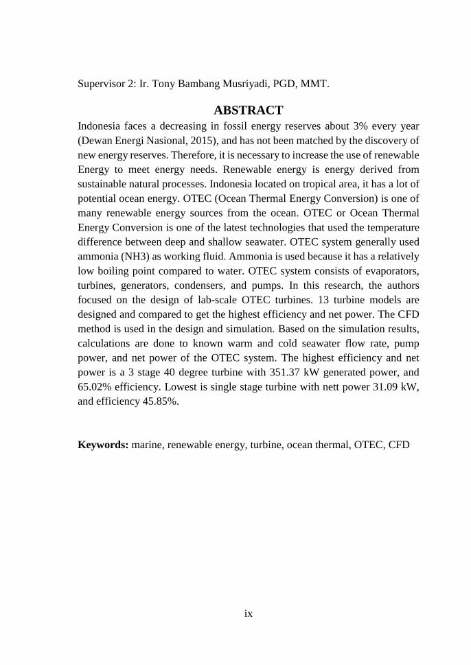
ABSTRACT
Indonesia faces a decreasing in fossil energy reserves about 3% every year
(Dewan Energi Nasional, 2015), and has not been matched by the discovery of
new energy reserves. Therefore, it is necessary to increase the use of renewable
Energy to meet energy needs. Renewable energy is energy derived from
sustainable natural processes. Indonesia located on tropical area, it has a lot of
potential ocean energy. OTEC (Ocean Thermal Energy Conversion) is one of
many renewable energy sources from the ocean. OTEC or Ocean Thermal
Energy Conversion is one of the latest technologies that used the temperature
difference between deep and shallow seawater. OTEC system generally used
ammonia (NH3) as working fluid. Ammonia is used because it has a relatively
low boiling point compared to water. OTEC system consists of evaporators,
turbines, generators, condensers, and pumps. In this research, the authors
focused on the design of lab-scale OTEC turbines. 13 turbine models are
designed and compared to get the highest efficiency and net power. The CFD
method is used in the design and simulation. Based on the simulation results,
calculations are done to known warm and cold seawater flow rate, pump
power, and net power of the OTEC system. The highest efficiency and net
power is a 3 stage 40 degree turbine with 351.37 kW generated power, and
65.02% efficiency. Lowest is single stage turbine with nett power 31.09 kW,
and efficiency 45.85%.
Keywords: marine, renewable energy, turbine, ocean thermal, OTEC, CFD

x
“This page is intentionally left blank”
Design and Simulation of Axial Turbine for Ocean Thermal
Energy Conversion (OTEC)
Name: Desta Rifky Aldara
NRP: 04211441000008
Supervisor 1: Irfan Syarif Arief, ST., MT.
Supervisor 2: Ir. Tony Bambang Musriyadi, PGD, MMT.

xi
ABSTRAK
Indonesia menghadapi penurunan cadangan energi fosil sekitar 3% setiap
tahun (Dewan Energi Nasional, 2015), dan belum diimbangi dengan penemuan
cadangan energi baru. Oleh karena itu, perlu untuk meningkatkan penggunaan
Energi terbarukan untuk memenuhi kebutuhan energi. Energi terbarukan
adalah energi yang berasal dari proses alam berkelanjutan. Indonesia terletak
di daerah tropis, memiliki banyak potensi energi laut. OTEC (Ocean Thermal
Energy Conversion) adalah salah satu dari banyak sumber energi terbarukan
dari lautan. OTEC atau Ocean Thermal Energy Conversion adalah salah satu
teknologi terbaru yang menggunakan perbedaan suhu antara air laut dalam dan
dangkal. Sistem OTEC umumnya menggunakan amonia (NH3) sebagai fluida
kerja. Amonia digunakan karena memiliki titik didih yang relatif rendah
dibandingkan dengan air. Sistem OTEC terdiri dari evaporator, turbin,
generator, kondensor, dan pompa. Dalam penelitian ini, penulis memfokuskan
pada desain turbin OTEC skala laboratorium. 13 model turbin dirancang dan
dibandingkan untuk mendapatkan efisiensi dan daya bersih tertinggi. Metode
CFD digunakan dalam desain dan simulasi. Berdasarkan hasil simulasi,
perhitungan dilakukan untuk mengetahui debit air laut hangat dan dingin, daya
pompa, dan daya bersih sistem OTEC. Efisiensi tertinggi dan daya bersih
adalah turbin 3 stage 40 derajat dengan 350,91 kW daya yang dihasilkan, dan
efisiensi 65,02%. Terendah adalah turbin satu tahap dengan daya nett 30,87
kW, dan efisiensi 45,85%.
Keywords: laut, energi terbarukan, turbin, panas laut, OTEC, CFD

xii
“This page is intentionally left blank”
PREFACE
Alhamdulillahirabbil ‘alamin, huge thanks to Allah SWT the God
Almighty for giving intelligent, strength, health and favours so the author can
finish this bachelor thesis.
This bachelor thesis aims to know how to design Otec turbine, and the
performance of its models. The author also would express his immeasureable
appreciation and deepest gratitudefor those who helpedin completing this
bachelor thesis:

xiii
1. The author’s parents Capt. Zaenal Mutaqin and Ibu Suwanti, author’s
siblings, and the whole family who always given motivation, support
and unceasingly prayer.
2. Dr. Eng . M. Badrus Zaman, S.T., M.T. as Head Department of Marine
Engineering.
3. Dr. Ing. Wolfgang Busse as Hochschule Wismar representative in
Indonesia.
4. Irfan Syarif Arief, ST., MT. and Ir. Tony Bambang Musriyadi, PGD,
MMT. as the author’s supervisor in this bachelor thesis who have
provided meaningful guidance, assistance, recommendation, and
motivation.
5. Ir. Aguk Zuhdi M.Fathallah., M.Eng., Ph.D as the author’s student
advisor who have provided meaningful guidance, assistance,
recommendation, and motivation.
6. Marine Manufacturing and Design laboratory staff who always
gossiping almost all people in the department.
7. Kaldam 75 squad who have rented Abah and Umi house for about 3
years.
8. The author’s beloved girl friends Dea Anggun Nabella Kimata who
always give support, motivation.
The author realizes that this thesis remains far away from perfect. Therefore,
every constructive suggestions and idea from all parties are highly expected by
the author to improve this bachelor thesis in future. Hopefully, this bachelor
thesis can be advantages for all of us, particularry the readers.
Surabaya, July 2018
Author

xiv
“This page is intentionally left blank”
Table of Contents
APPROVAL FORM ....................................... Error! Bookmark not defined.
APPROVAL FORM ....................................... Error! Bookmark not defined.
ABSTRACT ................................................................................................... ix

xv
ABSTRAK ..................................................................................................... xi
PREFACE ...................................................................................................... xii
Table of Contents ......................................................................................... xiv
List of Figure .............................................................................................. xviii
LIST OF TABLE .......................................................................................... xx
CHAPTER I INTRODUCTION .................................................................... 1
1.1 Background ....................................................................................... 1
1.2 Research Problem ............................................................................. 2
1.3 Research Limitation .......................................................................... 2
1.4 Research Objectives .......................................................................... 2
1.5 Research Benefit ............................................................................... 2
CHAPTER II LITERATURE STUDY ........................................................... 3
2.1 Preliminary ........................................................................................ 3
2.2 Ocean Thermal Energy Conversion (OTEC) .................................... 4
II.2.1. History of Ocean Thermal Energy Conversion (OTEC) ........... 4
II.2.2. Open Cycle OTEC ..................................................................... 6
II.2.3. Close Cycle OTEC .................................................................... 7
II.2.4. Hybrid Cycle OTEC .................................................................. 8
2.3 OTEC Structure ................................................................................ 9
2.4 Rankine Cycle ................................................................................... 9
2.5 Organic Rankine Cycle ................................................................... 12
2.6 Steam Turbine ................................................................................. 13
2.6.1 History of Steam Turbine ........................................................ 14
2.6.2 Classification of Steam Turbine .............................................. 16
2.6.3 Steps how to Design a Turbine ................................................ 18
2.6.4 Power Generated by Turbine ................................................... 18
2.6.5 Velocity Triangle of Turbine ................................................... 19
2.7 Heat Exchanger ............................................................................... 20

xvi
2.8 Pump ............................................................................................... 21
2.7.1 Pump Head .............................................................................. 21
2.7.2 Pump Power ............................................................................. 23
2.9 Computational Fluid Dynamics (CFD) ........................................... 24
CHAPTER III METHODOLOGY ................................................................ 25
3.1 Problem Identification ................................................................. 26
3.2 Literature Study ........................................................................... 26
3.3 Data Collecting and Planning ...................................................... 26
3.4 Design of Turbine in CFD Software ........................................... 26
3.5 Simulation ................................................................................... 29
3.6 Data Analysis .............................................................................. 29
3.7 Conclusion ................................................................................... 29
CHAPTER IV DATA ANALYSIS ............................................................... 31
4.1 Design and Drawing of OTEC’s Turbine ....................................... 31
4.1.1 Calculation of Working Fluid State ......................................... 31
4.1.2 Calculation of Blade’s Angle ................................................. 33
4.1.3 Drawing Process of OTEC's Turbine ...................................... 34
4.1.4 Mesh Generation ..................................................................... 39
4.1.1 Processing ................................................................................ 41
4.2 Performance of OTEC Turbine ....................................................... 44
4.2.1 Calculation of OTEC Turbine Power ...................................... 46
4.2.2 Calculation of Volume Flow Rate ........................................... 48
4.2.3 Calculation of Heat Exchanger ................................................ 51
4.2.4 Calculation of Pump ................................................................ 57
4.2.5 Calculation of Nett Power ....................................................... 69
CHAPTER V CONCLUSION ...................................................................... 73
5.1 Conclusion ...................................................................................... 73

xvii
5.2 Sugestion ......................................................................................... 73
REFERENCES .............................................................................................. 75
ATTACHMENT ............................................................................................ 77
Attachment 1. Table Properties of Ammonia ................................................ 79
Attachment 2. OTEC Turbine Models ......................................................... 83
Attachment 3. Simulation Parameter ............................................................. 93
Attachment 4. Convergence History ............................................................. 97

xviii
“This page is intentionally left blank”
List of Figure
Figure 1. Open Cycle OTEC ........................................................................... 7
Figure 2. Close Cycle OTEC ........................................................................... 8
Figure 3. Hybrid Cycle OTEC ......................................................................... 8
Figure 4. OTEC Shore & Off-Shore Base Structure ....................................... 9
Figure 5. Simple Rankine Plant ..................................................................... 10
Figure 6. T-S & P-V Diagram of Ideal Rankine Cycle ................................. 10
xix
Figure 7. Organic Rankine Cycle Components ............................................. 13
Figure 8. Steam Turbine ................................................................................ 13
Figure 9. Aeolopile ........................................................................................ 14
Figure 10. Branca’s Turbine .......................................................................... 15
Figure 11. De Laval Turbine ......................................................................... 15
Figure 12. Axial Steam Turbine .................................................................... 16
Figure 13. Radial Steam Turbine ................................................................... 16
Figure 14. Impulse and Reaction Turbine ..................................................... 17
Figure 15. Velocity Triangle ......................................................................... 19
Figure 16. Heat Echanger .............................................................................. 20
Figure 17. Pump ............................................................................................ 21
Figure 18. Methodology Chart ...................................................................... 25
Figure 19. Side View of Turbine models ...................................................... 27
Figure 20. Design of turbine single blade view ............................................. 28
Figure 21. Design of turbine full view .......................................................... 29
Figure 22. Close cycle OTEC System ........................................................... 31
Figure 23. Hub and Shroud Definition .......................................................... 35
Figure 24. Hub and Shroud value .................................................................. 35
Figure 25. Stream Surface Setup ................................................................... 36
Figure 26. Meridional view ........................................................................... 36
Figure 27. Parameter for stator ...................................................................... 37
Figure 28. Parameter for rotor ....................................................................... 37
Figure 29. Camber view of stator .................................................................. 37
Figure 30. Camber view of rotor ................................................................... 38
Figure 31. Single blade view ......................................................................... 38
Figure 32. Full blade view ............................................................................. 39
Figure 33. AutoGrid User Interface ............................................................... 40
Figure 34. Geometry Check........................................................................... 40
Figure 35. Blade row type for stator and rotor ............................................. 41
Figure 36. Mesh 3D Solid View .................................................................... 41
Figure 37. User Interface of NUMECA FINE Turbo .................................... 41
Figure 38. Boundary Condition Inlet ............................................................. 42
Figure 39. Boundary Condition Outlet .......................................................... 42
Figure 40. Mass Flow Graphic ...................................................................... 43
Figure 41. Efficiency Graphic ....................................................................... 43
Figure 42. Torque Graphic ............................................................................ 44

xx
Figure 43. Simulation Result ......................................................................... 44
Figure 44. Mass Flow Error ........................................................................... 45
Figure 45. Efficiency of OTEC’s Turbine ..................................................... 46
Figure 46. Efficiency of OTEC’s Turbine ..................................................... 47
Figure 47. Evaporator .................................................................................... 51
Figure 48. LMTD Correction Factor ............................................................. 52
Figure 49. Condenser ..................................................................................... 54
Figure 50. LMTD Correction Factor ............................................................. 55
Figure 51. Working Fluid Pipeline ................................................................ 57
Figure 52. Evaporator Pipeline ...................................................................... 61
Figure 53. Condenser Pipeline....................................................................... 65
Figure 54. Nett Power of OTEC’s Turbine ................................................... 70
LIST OF TABLE
Table 1. Ocean’s Renewable Energy Potential in Indonesia ........................... 3
Table 2. Carnot efficiency result ..................................................................... 4
Table 3. Achievment of OTEC ........................................................................ 5
Table 4. Number of Blades ............................................................................ 28
Table 5. Result of OTEC’s Turbine Simulation ............................................ 45
Table 6. Calculation of Turbine Power ......................................................... 46
Table 7. Result of Ammonia Volume Flow Rate Calculation ....................... 48

xxi
Table 8. Result of Warm Seawater Volume Flow Rate Calculation ............. 49
Table 9. Result of Cold Seawater Volume Flow Rate Calculation ............... 50
Table 10. Result of Evaporator Calculation .................................................. 53
Table 11. Result of Condenser Calculation ................................................... 56
Table 12. Calculation of Working Fluid Pump ............................................. 60
Table 13. Calculation of Evaporator Pump ................................................... 64
Table 14. Calculation of Condenser Pump .................................................... 68
Table 15. Power generated by generator ....................................................... 69
Table 16. Nett Power ..................................................................................... 69

xxii
“This page is intentionally left blank”

1
CHAPTER I
INTRODUCTION
1.1 Background
Energy has an important role in the achievement of social, economic and
environmental goals for sustainable development, and national economic
activities. Energy use in Indonesia is increasing rapidly in line with economic
growth and population growth. Dependence on fossil energy, especially
petroleum in the fulfilment of domestic consumption is still high, about 96%
(petroleum 48%, gas 18%, and coal 30%) of total national energy consumption
(National Energy Council, 2014). Indonesia faces a decreasing in fossil energy
reserves about 3% every year (Dewan Energi Nasional, 2015), and has not been
matched by the discovery of new energy reserves. Therefore, it is necessary to
increase the use of renewable Energy to meet energy needs. Renewable energy
is energy derived from sustainable natural processes.
Studies and projects on renewable energy sources have been actively
conducted around the world to solve the challenge of energy supply and
concomitant environmental issues. Among renewable energy sources, ocean
energy has been used in various approaches and is known as an eco-friendly
one. Indonesia located on tropical area, it has a lot of potency in ocean energy.
OTEC (Ocean Thermal Energy Conversion) is one of many renewable energy
sources from the ocean. As part of ocean energy development, OTEC (Ocean
Thermal Energy Conversion) system has been applied in the United States,
Europe, Japan, and other developed countries.
OTEC or Ocean Thermal Energy Conversion is one of the latest
technologies that used the temperature difference between deep and shallow
seawater that drive generators to produce electrical energy. The sunlight that
falls on the oceans is so strongly absorbed by the water that effectively all of
its energy is captured within a shallow "mixed layer" at the surface, 35 to 100
m thick, where wind and wave actions cause the temperature and salinity to be
nearly uniform. In the tropical oceans between approximately 15° north and
15° south latitude, the heat absorbed from the sun warms the water in the mixed
layer to a value near 28°C that is nearly constant day and night and from month
to month. The annual average temperature of the mixed layer throughout the
region varies from about 27°C to about 29°C. Beneath the mixed layer, the
water becomes colder as depth increases until at 800 to 1000 m (2500 to 3300
ft), a temperature of 4.4°C (Avery & Wu, 1995). This temperature does not
change dramatically throughout the year, with varying degrees due to weather
and seasonal changes, and the temperature difference between day and night
turns only has an effect of about 1°C (Soesilo, 2017).

2
Ocean Thermal Energy Conversion generating systems can be classified
into three categories: open cycles, closed cycles, and hybrid cycles. OTEC
closed cycle generally uses ammonia (NH3) as working fluid. Ammonia is
used because it has a relatively low boiling point compared to water. OTEC
system consists of evaporators, turbines, generators, condensers, and pumps.
In this research, the authors focused on the design of lab-scale OTEC turbines
to get the highest efficiency and net power.
1.2 Research Problem
Based on background mentioned above, it can be concluded some
problems of this final project are:
1. How to design a steam turbine for OTEC System?
2. How is the performance of the OTEC turbine that has been
simulated by CFD software?
1.3 Research Limitation
The limitations of the problems in this research are:
1. Focused only on design of OTEC turbine,
2. System are steady state,
3. Adiabatic,
4. RPM of turbine is 3000,
5. Radius of hub and shroud determined 0.06 m and 0.1 m,
6. This research used CFD software to simulated the turbine,
7. Does not include metallurgical analysis,
8. Does not include financial analysis.
1.4 Research Objectives
Based on problems mention above, the objectives of this research are:
1. To know how to design a steam turbine for OTEC System.
2. To know the performance of OTEC turbine that has been
simulated by CFD software
1.5 Research Benefit
This research is expected to give benefits to several parties. Benefits that
can be obtained from this research are:
1. Increase the knowledge of the author and readers about the
potential of the ocean as renewable energy source.
2. Provide Information to develop OTEC as a renewable, and
environmentally friendly power plant.
3
CHAPTER II
LITERATURE STUDY
2.1 Preliminary
Indonesia has a lot of energy resources, both in the fossil resources, and
renewable natural resources. In renewable natural resources, Indonesia has
excellent potential, one of them is maritime sector. Dewan Energi Nasional
(English: National Energy Council) has mapped the potential of ocean's
renewable energy as shown in Table 1.
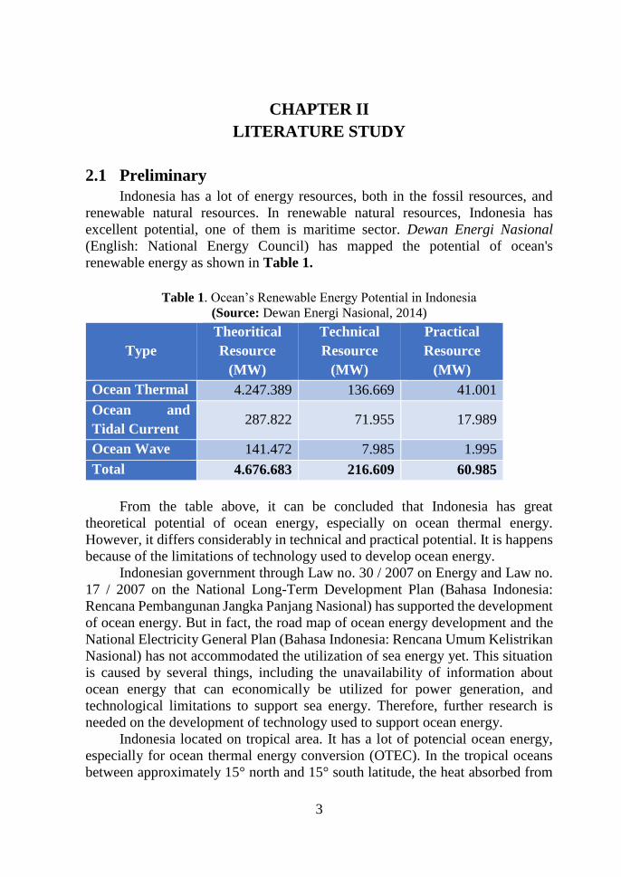
Table 1. Ocean’s Renewable Energy Potential in Indonesia
(Source: Dewan Energi Nasional, 2014)
Type
Theoritical
Resource
(MW)
Technical
Resource
(MW)
Practical
Resource
(MW)
Ocean Thermal 4.247.389 136.669 41.001
Ocean and
Tidal Current 287.822 71.955 17.989
Ocean Wave 141.472 7.985 1.995
Total 4.676.683 216.609 60.985
From the table above, it can be concluded that Indonesia has great
theoretical potential of ocean energy, especially on ocean thermal energy.
However, it differs considerably in technical and practical potential. It is happens
because of the limitations of technology used to develop ocean energy.
Indonesian government through Law no. 30 / 2007 on Energy and Law no.
17 / 2007 on the National Long-Term Development Plan (Bahasa Indonesia:
Rencana Pembangunan Jangka Panjang Nasional) has supported the development
of ocean energy. But in fact, the road map of ocean energy development and the
National Electricity General Plan (Bahasa Indonesia: Rencana Umum Kelistrikan
Nasional) has not accommodated the utilization of sea energy yet. This situation
is caused by several things, including the unavailability of information about
ocean energy that can economically be utilized for power generation, and
technological limitations to support sea energy. Therefore, further research is
needed on the development of technology used to support ocean energy.
Indonesia located on tropical area. It has a lot of potencial ocean energy,
especially for ocean thermal energy conversion (OTEC). In the tropical oceans
between approximately 15° north and 15° south latitude, the heat absorbed from

4
the sun warms the water. The annual average temperature of the surface layer
throughout the region varies from about 27°C to about 29°C.
Research conducted by Mega L. Syamsuddin (2014) on "OTEC Potential
in The Indonesian Seas" aims to identify and outline the potential and the position
of marine energy source that can be converted into electrical energy in Eastern
Indonesia by using and processing of secondary data obtained from satellites
(Syamsuddin et al., 2015). From the research get data as in Table 2.
Table 2. Carnot efficiency result
(Source: Mega L. Syamsuddin, 2014)
Location Tw
(°C)
Tc
(°C) ∆T Depth (m)
Carnot
Efficiency
South
Kalimantan
28.82 7.71 22.11 500 0.73
North
Sulawesi
29.22 7.44 21.78 500 0.74
Timur Strait 28.83 6.72 22.11 600 0.76
Makassar
Strait
28.83 6.72 22.11 600 0.76
South
Sulawesi
28.47 6.18 22.29 700 0.78
West Papua 28.16 6.76 21.4 600 0.75
Morotai Sea 28.47 6.82 21.65 600 0.76
From Table 2. can be concluded that potential OTEC in the Indonesian seas
is very large, based on some of the areas that have optimum temperature
conditions for ocean thermal energy conversion.
2.2 Ocean Thermal Energy Conversion (OTEC)
OTEC or Ocean Thermal Energy Conversion uses the temperature
difference between deep and shallow seawater that rotate generators to produce
electrical energy. OTEC power systems may be divided into three categories:
closed cycle, open cycle, and hybrid cycle. The three cycles are based on a
Rankine cycle of heat energy stored in the seawater into electrical energy (Avery
& Wu, 1995).
II.2.1. History of Ocean Thermal Energy Conversion (OTEC)
In 1870, the concept of ocean thermal energy conversion (OTEC), was
introduced by Jules Verne in Twenty Thousand Leagues Under the Sea.

5
Within a decade, American, French and Italian scientists are said to have been
working on the concept but the Frenchman, physicist Jacques-Arsene
d’Arsonval, is generally credited as the father of the concept for using ocean
temperature differences to create power. Table 3. provides a chronological
summary of important advances in OTEC technology.
Table 3. Achievment of OTEC
(Source: Kobayashi et al, )
Years Achievement
1881 Mr. J. D'Arsonval developed his idea of OTEC theory
1926 G.Claude (France) started experiments of OTEC
1933 Mr. G. Claude generated a net 12 kW output OTEC near
Cuba
1964 Anderson (USA) presented a proposal of Off-shore type
OTEC
1970 New Energy Research Committee researched OTEC
technology (JAPAN
1974 ERDA project started to research OTEC (USA)
1974 First OTEC conference was held (USA)
1977 Saga University succeeded with 1 kW experimental plant
1979 “Mini-OTEC” used cold-water pipe to produce 15kW power
(52kW gross)
1980 U.S. DOE built a test site for closed-cycle OTEC heat
exchangers, OTEC-1. Results showed that OTEC systems
can operate from floating platforms with little effect on the
marine environment. The same year 2 laws were enacted to
promote OTEC development: Ocean Thermal Energy
Conversion Act and Ocean Thermal Energy Conversion
Research, Development, and Demonstration Act.
1981 Tokyo Electric Co., and its subsidiary undertook successful
experiment of a 120 kW OTEC in Nauru. Used cold-water
pipe on the sea bed at 580m depth. Freon was the working
fluid. Produced 31.5 kW of net power.
1984 DOE developed a vertical-spout evaporator that converts
warm seawater to steam with efficiencies as high as 97%
1985 A 75 kW experimental OTEC plant was installed at Saga
University.
6
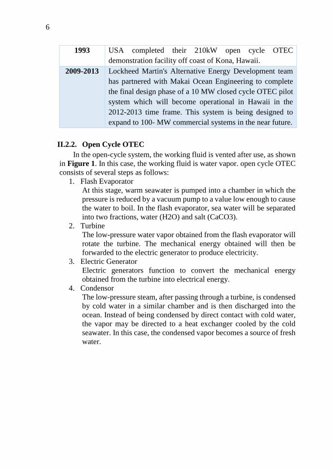
1993 USA completed their 210kW open cycle OTEC
demonstration facility off coast of Kona, Hawaii.
2009-2013 Lockheed Martin's Alternative Energy Development team
has partnered with Makai Ocean Engineering to complete
the final design phase of a 10 MW closed cycle OTEC pilot
system which will become operational in Hawaii in the
2012-2013 time frame. This system is being designed to
expand to 100- MW commercial systems in the near future.
II.2.2. Open Cycle OTEC
In the open-cycle system, the working fluid is vented after use, as shown
in Figure 1. In this case, the working fluid is water vapor. open cycle OTEC
consists of several steps as follows:
1. Flash Evaporator
At this stage, warm seawater is pumped into a chamber in which the
pressure is reduced by a vacuum pump to a value low enough to cause
the water to boil. In the flash evaporator, sea water will be separated
into two fractions, water (H2O) and salt (CaCO3).
2. Turbine
The low-pressure water vapor obtained from the flash evaporator will
rotate the turbine. The mechanical energy obtained will then be
forwarded to the electric generator to produce electricity.
3. Electric Generator
Electric generators function to convert the mechanical energy
obtained from the turbine into electrical energy.
4. Condensor
The low-pressure steam, after passing through a turbine, is condensed
by cold water in a similar chamber and is then discharged into the
ocean. Instead of being condensed by direct contact with cold water,
the vapor may be directed to a heat exchanger cooled by the cold
seawater. In this case, the condensed vapor becomes a source of fresh
water.

7
Figure 1. Open Cycle OTEC
(Source: http://www.zoombd24.com/ocean-thermal-energy-conversion-otec-system-
working-principles-and-efficiency/)
II.2.3. Close Cycle OTEC
In closed-cycle operation, the working fluid is conserved (i.e., pumped
back to the evaporator after condensation), as shown in Figure 2. Ammonia
is commonly used in this cycle because it has a relatively low boiling point
with seawater as a fluid to evaporate and condense. close cycle OTEC
consists of several steps as follows:
1. Evaporator
In the evaporator, seawater warm temperature about 26-30°C will
meet with ammonia or other working fluids. There is a heat transfer
between the two fluids that causes ammonia to evaporate into high-
pressure steam.
2. Turbine
The high pressure vapor ammonia will then through the turbine and
rotate the blades in the turbine.
3. Electric Generator
Electric generators function to convert the mechanical energy
obtained from the turbine into electrical energy.
4. Condensor
Ammonia vapor that passes through the turbine will get a decrease
in temperature and pressure which then continues into the
condenser. In the condenser there will be heat transfer between
ammonia vapor and cold seawater so that condensation occurs and
the ammonia phase changes become saturated liquid.

8
5. Working Fluid’s Pump
The ammonia passes through condenser will be pumped at a certain
pressure toward the evaporator.
Figure 2. Close Cycle OTEC
II.2.4. Hybrid Cycle OTEC
A hybrid cycle combines the features of the closed- and open-cycle
systems. In a hybrid, warm seawater enters a vacuum chamber and is flash-
evaporated, similar to the open-cycle evaporation process. The steam
vaporizes the ammonia working fluid of a closed-cycle loop on the other side
of an ammonia vaporizer. The vaporized fluid then drives a turbine to
produce electricity. The steam condenses within the heat exchanger and
provides desalinated water.
Figure 3. Hybrid Cycle OTEC
(Source: http://proyectos2.iingen.unam.mx/IIDEA/otec_plants.html)

9
2.3 OTEC Structure
Ocean Thermal Energy Conversion (OTEC) has 2 types of building
structures, which are shore-based and off-shore based. The shore-based structure
has three main advantages over those located in deep water. Plants constructed on
shore do not require sophisticated mooring, lengthy power cables, or the more
extensive maintenance associated with open-ocean environments. they can be
installed in a sheltered area and relatively save from heavy storm and wave. The
shore-based structure also can be integrated with cooling system around plants,
desalinated system, and mariculture. Off-shore based structures installed floating
in the sea. They have potentially optimal for large systems but has difficultness
such as on mooring system, and delivery power system.
Figure 4. OTEC Shore & Off-Shore Base Structure
(Source: http://www.makai.com/images/Offshore_OTEC_Diagram_900x489.png)
2.4 Rankine Cycle
The Rankine cycle closely describes the process by which steam-operated
heat engines commonly found in thermal power plants. This cycle used two
phases of working fluid, there are liquid and vapour. in a simple Rankine cycle
consists of 4 main components namely condenser, pump, boiler, and turbine as
shown in Figure 5. The difference of OTEC power plant and thermal power plant
is the boiler replaced by evaporator and the boiling point of OTEC cycle is lower
so that water is not suitable for working fluid.
10
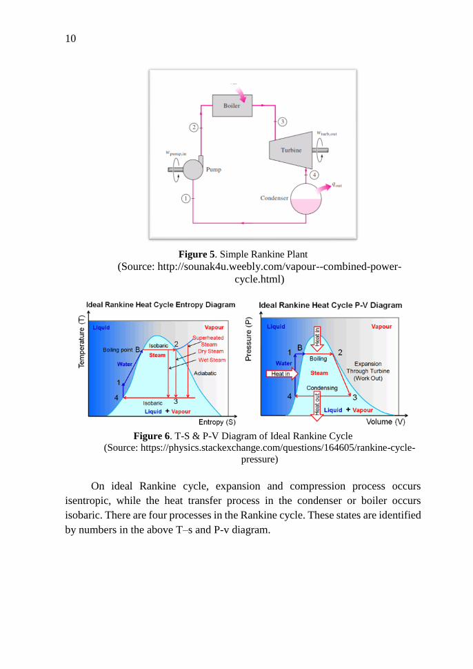
Figure 5. Simple Rankine Plant
(Source: http://sounak4u.weebly.com/vapour--combined-power-
cycle.html)
Figure 6. T-S & P-V Diagram of Ideal Rankine Cycle
(Source: https://physics.stackexchange.com/questions/164605/rankine-cycle-
pressure)
On ideal Rankine cycle, expansion and compression process occurs
isentropic, while the heat transfer process in the condenser or boiler occurs
isobaric. There are four processes in the Rankine cycle. These states are identified
by numbers in the above T–s and P-v diagram.

11
• 1-2: Heat transfer process to the working fluid from the boiler with
constant pressure (isobaric)
• 2-3: An isentropic expansion occurs on the fluid through the turbine
from the superheated state to the condenser pressure.
• 3-4: Heat transfer process of working fluid flowing with constant
pressure (isobaric) on condenser to saturated liquid in state 4
• 4-1: The isentropic compression process at the pump where from the
saturated liquid state to the compression liquid state.
In the design of the turbine states, if the working fluid conditions inlet (T1,
P1) and outlet (T2, P2) are known, then the inlet enthalpy and entropy can be found
by using the properties table. The ideal state (s2s = s1) of the system can be
calculated by using the equation (Reynolds & Perkins, 1989):
𝑠2𝑠 = 𝑠𝑓 + 𝑥2𝑠(𝑠𝑔−𝑠𝑓) .................................................... (2-1)
ℎ2𝑠 = ℎ𝑓 + 𝑥2𝑠. ℎ𝑓𝑔 ......................................................... (2-2)
𝑥2𝑠 =𝑠1−𝑠𝑓
𝑠𝑔−𝑠𝑓 ....................................................................... (2-3)
Where:
S2s = Entropi ideal state (kj/kg.K)
Sf = Entropi saturated liquid (kj/kg.K)
Sg = Entropi saturated gas (kj/kg.K)
h2s = Entalpi ideal state (kj/kg)
hf = Entalpi saturated liquid (kj/kg)
hg = Entalpi saturated gas (kj/kg)
x = Gas quality
The real states can be calculated by using the equation:

12
ℎ2 = ℎ1 − 𝜂𝑡(ℎ1 − ℎ2𝑠) (2-4)
𝑥2 =ℎ2−ℎ𝑓
ℎ𝑓𝑔 (2-5)
𝑠2 = 𝑠𝑓 + 𝑥(𝑠𝑔−𝑠𝑓) (2-6)
𝑊ℎ𝑒𝑟𝑒
S2 = Entropi real state (kj/kg.K)
Sf = Entropi saturated liquid (kj/kg.K)
Sg = Entropi saturated gas (kj/kg.K)
h2 = Entalpi real state (kj/kg)
hf = Entalpi saturated liquid (kj/kg)
hg = Entalpi saturated gas (kj/kg)
x = Gas quality
ηt = Isentropic efficiency
2.5 Organic Rankine Cycle
Organic Rankine Cycle is a modified energy conversion process from
Rankine Cycle. Rankine Cycle usually use pressurized and high-temperature
water as a working fluid. While in ORC, the boiling point of this cycle is lower
so that water is not suitable for working fluid. Therefore, hydrocarbons or
refrigerants are used which have low boiling point as working fluids. The main
component of the ORC are condenser, pump, evaporator, and turbine as shown in
Figure 7.

13
Figure 7. Organic Rankine Cycle Components
(Source: http://www.tocircle.com/applications/energy-efficiency/organic-
rankine-cycle/)
2.6 Steam Turbine
Figure 8. Steam Turbine
(Source: https://www.fujielectric.com/products/thermal_power_generation/)
Figure 8. shown the steam turbine. A turbine is a rotary mechanical device
that extracts energy from a fluid flow and converts it into useful work. The
rotating part is the rotor, while the non-rotating part is the stator or turbine
housing. A turbine is a turbomachine with at least one moving part called a rotor
assembly, which is a shaft or drum with blades attached. Moving fluid acts on the
blades so that they move and impart rotational energy to the rotor. The work
produced by a turbine can be used for rotating the load (i.e. electrical generator,
pump, compressor, propeller, etc.). The working fluid may be water, steam, or gas
(Arismunandar, 2004).

14
The closed OTEC cycle is basically the same as the conventional Rankine
cycle employed in steam engines, in which the steam is condensed and returned
to the boiler after driving a piston or steam turbine. OTEC differs by using a
different working fluid and lower pressures and temperatures(Avery & Wu,
1995).
Steam turbine is a driving force that converts steam potential energy into
kinetic energy and then converted into mechanical energy in the form of turbine
spinning. Turbine axle, directly or with reduction gear, connected with the
mechanism to be driven.
2.6.1 History of Steam Turbine
The idea of steam turbine was proposed by Hero of Alexandria, during the
1st century CE. Hero of Alexandria created the first prototypes of turbine
called aeolipile as shown in Figure 8 by the reaction principle. In this device,
steam was supplied through a hollow rotating shaft to a hollow rotating
sphere. It then emerged through two opposing curved tubes, just as water
issues from a rotating lawn sprinkler. The device was little more than a toy,
since no useful work was produced.
Another steam-driven machine, proposed by Giovanni Branca in 1629 in
Italy, was designed in such a way that a jet of steam impinged on blades
extending from a wheel and caused it to rotate by the impulse principle, as
shown in Figure 9. Patent by James Watt in 1784 starting the developer of
the steam engine, a number of reaction and impulse turbines were proposed,
all adaptations of similar devices that operated with water.
Figure 9. Aeolopile
(Source: http://c8.alamy.com/comp/BFB238/herons-aeolipile-BFB238.jpg)

15
Figure 10. Branca’s Turbine
(Source: http://c8.alamy.com/comp/BFB238/herons-aeolipile-BFB238.jpg)
Small reaction turbines that turned at about 40,000 RPM to drive cream
separators constructed by Carl G.P. de Laval of Sweden during 1880s. Their
high speed, however, made them unsuitable for other commercial
applications. From 1889 to 1897 de Laval built many turbines with capacities
from about 15 to hundred horsepower. His 15-horsepower turbines were the
first employed for marine propulsion (1892). in 1890s, C.E.A. Rateau of
France developed multistage impulse turbine. At about the same time, the
velocity-compounded impulse stage was developed by Charles G. Curtis of
the United States.
Figure 11. De Laval Turbine
(Source: https://www.britannica.com/technology/turbine/History-of-steam-
turbine-technology)
16
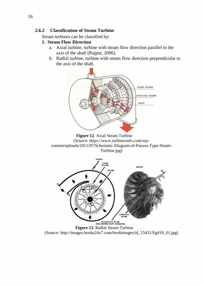
2.6.2 Classification of Steam Turbine
Steam turbines can be classified by:
1. Steam Flow Direction
a. Axial turbine, turbine with steam flow direction parallel to the
axis of the shaft (Rajput, 2006).
b. Radial turbine, turbine with steam flow direction perpendicular to
the axis of the shaft.
Figure 12. Axial Steam Turbine
(Source: https://www.turbinesinfo.com/wp-
content/uploads/2011/07/Schematic-Diagram-of-Parson-Type-Steam-
Turbine.jpg)
Figure 13. Radial Steam Turbine
(Source: http://images.books24x7.com/bookimages/id_15431/fig418_01.jpg)

17
2. The principle used to rotate the turbine wheel through the blade
a. Impulse Turbine
Impulse turbines change the direction of flow of a high-velocity
fluid or gas jet. The resulting impulse spins the turbine and leaves
the fluid flow with diminished kinetic energy. There is no pressure
change of the fluid or gas in the turbine blades (the moving blades),
all the pressure drop takes place in the stationary blades (the
nozzles). Impulse turbines are most efficient for use in cases where
the flow is low and the inlet pressure is high (Rubenstein, Yin, &
Frame, 2012).
b. Reaction Turbine
Reaction turbines develop torque by reacting to the gas or fluid's
pressure or mass. The pressure of the gas or fluid changes as it
passes through the turbine rotor blades. Reaction turbines are better
suited to higher flow velocities or applications where the fluid head
(upstream pressure) is low.
Figure 14. Impulse and Reaction Turbine
(Source: http://www.mech4study.com/2015/12/difference-between-impulse-
and-reaction-turbine.html)
3. Steam Pressure
a. Low pressure turbines, using steam at a pressure of 1.2 to 2 ata.
b. Medium pressure turbines, using steam at pressure up to 40 ata.
c. High pressure turbines, utilising steam at pressure above 40 ata.
18
d. Turbines of very high pressure, utilising steam at pressure of 170
ata and higher.
e. Turbines of supercritical pressure, using steam at pressure above
225 ata.
2.6.3 Steps how to Design a Turbine
To design a single stage turbine, it takes several steps (Shlyakhin, 1999),
including:
1. Determining the capacity/power
2. Determining rotation per minutes
3. Determining temperature and pressure inlet
4. Determining pressure outlet
2.6.4 Power Generated by Turbine
Steam turbine is designed by a certain power. The power generated by
the turbine is obtained from the difference in enthalpy and the steam capacity
entering the turbine, and losses inside the turbine due to energy
transformation. The power generated by the turbine can be determined by
using the formula (Dietzel & Sriyono, 1996):
𝑃 = ℎ. ṁ𝑠. 𝜂𝑖 . 𝜂𝑚 ........................................ (2-7)
Where:
P = Power (kW)
h = Difference of entalpi (KJ/Kg)
ṁs = Steam Capacity (Kg/s)
ηi = Internal efficiency of the turbine
ηm = Mechanical efficiency of the turbine (0,94-0,97)
If the torque and RPM of turbine are known, then turbine power can be
calculated using the equation:
𝑃 = 𝑇 × 2𝜋 × 𝑅𝑃𝑀/60000 ...................... (2-8)
Where:
P = Power (kW)
T = Torque (Nm)
RPM = Revolution per minutes

19
2.6.5 Velocity Triangle of Turbine
In the steam turbine, vapor is expanded in the nozzle so, obtained the
vapor velocity (c1) that will enter to the rotor on turbine. The rotor rotates
with the velocity u. It needs c1 and u ratio with a certain value so that the
steam flow out of the nozzle works optimally. Thus, can be obtained inlet and
outlet angle (Dietzel & Sriyono, 1996). Velocity triangle can be seen in
Figure 14.
Figure 15. Velocity Triangle
(Source: Dietzel, 1996)
Angle α1 and β1 shall be made in such a way, according to the vapor
velocity. Value of α1 is free to determined, but should be as small as possible.
The optimum value of α1 is between 14°-20° (Shlyakhin, 1999). From α1 can
be found:
𝑤1 = √𝐶12 + 𝑢2 − 2. 𝐶1. 𝑢. cos 𝛼1 ........................ (2-9)
𝛽1 =𝐶1
𝑤1× 𝛼1 .......................................................... (2-10)
𝛽2 = 𝛽1 − (3° − 5°) .............................................. (2-11)
𝑤2 = Ψ × 𝑤1 .......................................................... (2-12)
𝐶2 = √𝑤22 + 𝑢2 − 2. 𝑤2. 𝑢. cos 𝛽2 ........................ (2-13)
𝑆𝑖𝑛 𝛼2 =𝑤2
𝐶2 ............................................................ (2-14)
Where:
c1 and c2 : absolute velocity of steam inlet and outlet from the nozzle
w1 and w2 : relative velocity of steam inlet and outlet from the rotating blades
u : circumference velocity of the rotating blade
α1 and α2 : angle of the nozzle
β1 and β2 : angle of the rotating blades
Ψ : speed coefficient

20
2.7 Heat Exchanger
Figure 16. Heat Echanger
Heat exchanger used to transfer heat between two or more fluids. The fluids
separated by a solid wall to prevent mixing or they may be in direct contact. They
are usually used in space heating, refrigeration, air conditioning, power stations,
chemical plants, petrochemical plants, petroleum refineries, natural-gas
processing, and other. In OTEC system used heat exchanger that is evaporator
and condenser. evaporator replace the boiler function in the steam power plant.
An evaporator used to turn the liquid form of a chemical substance such as water
into its gaseous-form/vapor. A condenser used to condense a substance from its
gaseous to its liquid state, by cooling it. The design calculation for heat exchange
means is essentially determining the heat transfer coefficient and heat transfer
area (A) of the following equations (Holman, 2010):
𝐴 =𝑄
𝑈×𝐿𝑀𝑇𝐷×𝐹 ......................................................................... (2-15)
𝑄 = ṁ𝑊𝑎𝑟𝑚 × 𝐶𝑝𝑊𝑎𝑟𝑚 × ∆𝑇 ................................................. (2-16)
𝐿𝑀𝑇𝐷 =(𝑇ℎ,𝑖𝑛−𝑇𝑐,𝑜𝑢𝑡)−(𝑇ℎ,𝑜𝑢𝑡−𝑇𝑐,𝑖𝑛)
ln[ (𝑇ℎ,𝑖𝑛−𝑇𝑐,𝑜𝑢𝑡)
(𝑇ℎ,𝑜𝑢𝑡−𝑇𝑐,𝑖𝑛)]
......................................... (2-17)
Where:
A = Area (m2)
Q = Heat transfer rate (Watt)
U = The overall heat transfer coefficient (W/m2.oC)
LMTD = Logarithmic mean temperature difference (oC)
F = LMTD correction factor
21
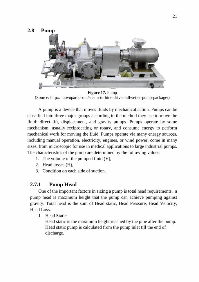
2.8 Pump
Figure 17. Pump
(Source: http://nuovoparts.com/steam-turbine-driven-allweiler-pump-package/)
A pump is a device that moves fluids by mechanical action. Pumps can be
classified into three major groups according to the method they use to move the
fluid: direct lift, displacement, and gravity pumps. Pumps operate by some
mechanism, usually reciprocating or rotary, and consume energy to perform
mechanical work for moving the fluid. Pumps operate via many energy sources,
including manual operation, electricity, engines, or wind power, come in many
sizes, from microscopic for use in medical applications to large industrial pumps.
The characteristics of the pump are determined by the following values:
1. The volume of the pumped fluid (V),
2. Head losses (H),
3. Condition on each side of suction.
2.7.1 Pump Head
One of the important factors in sizing a pump is total head requirements. a
pump head is maximum height that the pump can achieve pumping against
gravity. Total head is the sum of Head static, Head Pressure, Head Velocity,
Head Loss.
1. Head Static
Head static is the maximum height reached by the pipe after the pump.
Head static pump is calculated from the pump inlet till the end of
discharge.
22
2. Head Pressure
Head Pressure is the diference of pressure on the suction and
discharge.
3. Head Velocity
Head Velocity is difference velocity of fluid between in suction and
discharge of pump.
4. Head Loss
Head loss is energy loss per unit weight of the fluid in the drainage of
fluid in the piping system. Head Losses including head major and head
minor in suction and discharge.
• Head Major
Major losses are associated with frictional energy loss per length
of pipe depends on the flow velocity, pipe length, pipe diameter,
and a friction factor based on the roughness of the pipe, and
whether the flow is laminar or turbulent. Head Major can be
calculated with the equation:
𝑀𝑎𝑗𝑜𝑟 𝑙𝑜𝑠𝑠𝑒𝑠 =𝑓×𝐿×𝑣2
𝑑×2𝑔 ............................... (2-18)
Where:
f = the Darcy friction factor (unitless)
L = the pipe length (m)
d = the hydraulic diameter of the pipe D (m)
g = the gravitational constant (m/s2)
v = the mean flow velocity V (m/s)
The value of the Darcy friction factor is determined from the flow
type (ie laminar or turbulent), with the equation:
𝑓 = 0.02 + 0.0005/𝑑 (Turbulent Re>2300) ................ (2-19)
𝑓 =64
𝑅𝑒 (Laminar Re<2300) ........................................... (2-20)
𝑅𝑒 =𝑣×𝑑
𝜇 ....................................................................... (2-21)

23
Where:
Re = Reynold Number
v = flow velocity (m/s)
d = inner diameter of pipe (m)
μ = kinematis viscosity (m2/s)
• Head Minor
Minor loss is a pressure loss in components like valves, bends,
tees and similar. Head minor can be calculated with the equation:
𝑀𝑖𝑛𝑜𝑟 𝐿𝑜𝑠𝑠𝑒𝑠 =Ʃ𝑛𝑘×𝑣2
2𝑔 ............................... (2-22)
Where:
Ʃnk = Minor loss coefficient
2.7.2 Pump Power
As described in the previous section, the total head has an effect on the size
of the pump and the driving machine. The pump power is the power that can be
used to move the fluid and drive the driving machine. Pump power can be
calculated by using equation:
𝑃 = ρ × Q × g × H𝑡𝑜𝑡𝑎𝑙 ................................ (2-23)
Where:
P = Power (Watt)
ρ = Density (kg/m3)
Q = Volume flow rate (m3/s)
g = the gravitational constant (m/s2)
Htotal = Total head (m)

24
2.9 Computational Fluid Dynamics (CFD)
Computational fluid dynamics (CFD) is a branch of fluid mechanics that uses
numerical analysis and data structures to solve and analyze problems that involve
fluid flows. Computers are used to perform the calculations required to simulate
the interaction of liquids and gases with surfaces defined by boundary conditions
(CFD-Online, n.d.).
In the simulation process, there are three steps that must be done, there are
pre-processing, solving and post-processing.
1. Pre-Processor
Pre-processor is the initial stage in Computational Fluid Dynamic (CFD)
which is the stage of data input that includes the determination of domain
and boundary condition. At this stage, meshing is also done, where the
analyzed object is divided into the number of specific grids.
2. Processor
The next step is the processor stage. At this stage, is done the process of
calculating data that has been entered using iterative related equations until
the results obtained can reach the smallest error value.
3. Post Processor
The last step is the post processor stage, the results of the calculations at the
processor stage will be displayed in pictures, graphs and animations.

25
CHAPTER III
METHODOLOGY
Methodology represents the completion steps in this study. Problem solving
in this research used Computational Fluid Dynamics method. The steps of this
methodology are as follows as in Figure 18.
Figure 18. Methodology Chart

26
3.1 Problem Identification
The first step in this final project is identifying the problem. The selection of
the topic starts from Indonesia faces a decreasing in fossil energy reserves and
Indonesia's dependence on fossil energy which is not been matched by the
discovery of new energy reserves. Therefore, it is necessary to increase the use of
renewable Energy to meet energy needs. One of many renewable energies is
OTEC. The important component of the Ocean Thermal Energy Conversion
(OTEC) system is the turbine, therefore further research is needed on OTEC
turbine optimization.
3.2 Literature Study
Literature study aims to get a summary of the basics of existing theories,
references and various information that can be a supporter in this final project.
Literature study was conducted by collecting references to be studied as
supporting materials for research activities such as books, journals, papers or from
internet. In addition, it can also discussing with competent persons in this field.
The literature studied is closely related to: Ocean Thermal Energy Conversion
(OTEC), Steam Turbine, Heat Exchanger, Pump, and Computational Fluid
Dynamics (CFD).
3.3 Data Collecting and Planning
At this stage will be data collection and planning for Ocean Thermal Energy
Conversion (OTEC) turbine, the required data are shallow and deep water
temperature in order to know the potential of OTEC in Indonesia that will be used
as reference for turbine planning. Data obtained from research conducted by Mega
L. Syamsuddin (2014) on "OTEC Potential in The Indonesian Seas" the average
temperature of shallow and deep water temperature are 28.68°C and 6.9°C with
the difference reaching 21.78°C at a depth 500 – 700m. From the data assumed
the inlet and outlet of temperature and pressure of turbine are:
Tin : 24°C
Pin : 9.7274 bar
Tout : 10°C
Pout : 6.1529 bar
3.4 Design of Turbine in CFD Software
After the blade’s angle calculation, then the next step is to design turbine into
3D form by using the software. In this research, 13 variations of turbine model
will be made, that are: Single Stage, 2 Stage, 2 Stage 5 Degree, 2 Stage 10 Degree,
2 Stage 15 Degree, 2 Stage 20 Degree, 2 Stage 25 Degree, 2 Stage 30 Degree, 2
Stage 35 Degree, 2 Stage 40 Degree, 2 Stage 45 Degree, 2 Stage 50 Degree, 3

27
Stage 40 Degree. Figure 19. Is a side view of the turbine model. The number of
turbine blades can be seen on Table 4.
Figure 19. Side View of Turbine models

28
Table 4. Number of Blades
Name Row Number of Blades
Single Stage 1 10
2 15
2 Stage
1 10
2 15
3 15
4 20
3 Stage
1 10
2 15
3 15
4 20
5 20
6 25
In this study, the software used to design the turbine is Autoblade.Design of
turbine as shown in Figure 20. single blade view and Figure 21. Full blade view
for single stage turbine. The other OTEC turbine model, it can be seen in
Attachment 2.
Figure 20. Design of turbine single blade view
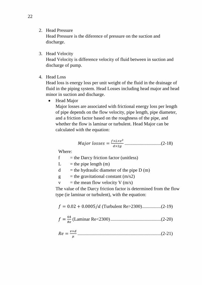
29
Figure 21. Design of turbine full view
3.5 Simulation
Simulation and modification of model is done by using Computational Fluid
Dynamics (CFD) software. In this research, the turbine model is simulated and
will be compared to get the highest efficiency and net power.
3.6 Data Analysis
The data has been obtained from the simulation process, then do the
calculation of heat exchanger, pump power, and net power, analyzed and
compared the efficiency.
3.7 Conclusion
The last step in this final project is making conclusion. The conclusion based
on the results of simulation and analysis. This conclusion is prepared to answer
the research problem.

30
“This page is intentionally left blank”

31
CHAPTER IV
DATA ANALYSIS
Figure 22. Close cycle OTEC System
OTEC system consists of turbines, generators, evaporators, condensers, and
pumps as shown on Figure 22. In this chapter will explain how to design Ocean
Thermal Energy Conversion (OTEC) turbine, simulation of turbine design, heat
exchanger calculation, pump calculation, and net power calculation to be
delivered to the consumer.
4.1 Design and Drawing of OTEC’s Turbine
In this sub-chapter will be explaining the design process using Autoblade
software and simulation process using NUMECA Fine Turbo software. The first
process is to determine the working fluid state at the inlet and outlet of OTEC's
turbine, then, determining the angle of the turbine blades, and the last is the
drawing of OTEC's turbines by using Autoblade software.
4.1.1 Calculation of Working Fluid State
Data obtained from research conducted by Mega L. Syamsuddin (2014)
on "OTEC Potential in The Indonesian Seas" the average temperature of

32
shallow and deep water temperature are 28.68°C and 6.9°C with the difference
reaching 21.78°C at a depth 500 – 700m. From the data assumed the inlet and
outlet of temperature and pressure of turbine are:
Tin : 24°C
Pin : 9.7274 bar
Tout : 10°C
Pout : 6.1529 bar
Then, State 1 is found after the working fluid exits the evaporator. From
the ammonia table properties Attachment 1 we get:
P1 : 9.7274 bar
T1 : 24°C
h1 : 1462.61 kJ/kg
s1 : 5.0394 kJ/kg.K
State 2 is found after the working fluid flow through the turbine can be
determined by equation 2.1-2.7 :
P2 : 6.1529 bar
T2 : 10°C
State s2s = s1
• 𝑠2𝑠 = 𝑠𝑓 + 𝑥(𝑠𝑔−𝑠𝑓) → 𝑥2𝑠 =𝑠1−𝑠𝑓
𝑠𝑔−𝑠𝑓
𝑥2𝑠 =5.0394 − 0.8769
5.2033 − 0.8769= 0.962116
𝑠2𝑠 = 0.8769 + 0.962116(5.2033 − 0.8769)
= 5.0394 kJ/kg. K
• ℎ2𝑠 = ℎ𝑓 + 𝑥. ℎ𝑓𝑔
ℎ2𝑠 = 226.75 + 0.962116 × 1225.03 = 1402.371kJ/kg
• 𝜂𝑡 =ℎ1−ℎ2
ℎ1−ℎ2𝑠= 50% (assumption)
Isentropic efficiency for turbine as low as 40% (Agency, 2015)
• ℎ2 = ℎ1 − 𝜂𝑡(ℎ1 − ℎ2𝑠)
ℎ2 = 1462.61 − 50% × (1462.61 − 1405.371)
ℎ2 = 1433.991 kJ/kg
• 𝑥2 =ℎ2−ℎ𝑓
ℎ𝑓𝑔
𝑥2 =1433.997 − 226.75
1225.03= 0.9855
• 𝑠2 = 𝑠𝑓 + 𝑥(𝑠𝑔−𝑠𝑓)
𝑠2 = 0.8769 + 0.9855(5.2033 − 0.8769) = 5.1404 kJ/kg. K

33
From the calculation above, can be found:
State 1 is found after the working fluid exits the evaporator:
P1 : 9.7274 bar
T1 : 24°C
h1 : 1462.61 kJ/kg
s1 : 5.0394 kJ/kg.K
State 2 is found after the working fluid flow through the turbine can be
determined:
P2 : 6.1529 bar
T2 : 10°C
h2 : 1433.997 kJ/kg
s2 : 5.1404 kJ/kg.K
4.1.2 Calculation of Blade’s Angle
The angle of the turbine blades is designed so as to produce optimum work
on the turbine. Value of α1 is free to determined, but should be as small as
possible. The optimum value of α1 is between 14°-20° (Shlyakhin, 1999). In
this research, the value of α1 = 15 °. Following is the calculation of blade’s
angle:
• 𝛼1 = 15°
• 𝐶1𝑡 = 44.72 × √∆ℎ
𝐶1𝑡 = 44.72 × √1462.61 − 1433.991 = 239.24 m/s
• 𝐶1 = 𝜑. 𝐶1𝑡
𝐶1 = 0.95 × 239.24 = 227.28 m/s
Range of 𝜑 is between 0.91-0.98 (usually use 0.95)
• 𝑢 = (𝑢
𝑐1) × 𝑐1
𝑢 = (0.4) × 227.28 = 90.91 𝑚/𝑠
Value of (𝑢
𝑐1) for single stage turbine is between 0.2-0.6, optimal
value is 0.4 (Shlyakhin, 1999).
• 𝑤1 = √𝐶12 + 𝑢2 − 2. 𝐶1. 𝑢. cos 𝛼1
𝑤1 = √227.282 + 90.912 − 2 × 227.28 × 90.91 × cos 15°
𝑤1 = 141.4 𝑚/𝑠

34
• 𝛽1 =𝐶1
𝑤1× 𝛼
𝛽1 =227.28
141.4× 15° = 24.1°
• 𝛽2 = 𝛽1 − (3° − 5°)
𝛽2 = 𝛽1 − (3°) = 21.1°
• 𝑤2 = Ψ × 𝑤1 (Ψ = 0.45) (Dietzel & Sriyono, 1996) page 94)
𝑤2 = 0.45 × 141.4
𝑤2 = 63.65 𝑚/𝑠
• 𝐶2 = √𝑤22 + 𝑢2 − 2. 𝑤2. 𝑢. cos 𝛽2
𝐶2 = √63.652 + 90.912 − 2 × 63.65 × 90.91 × cos 21.1
𝐶2 = 38.98 𝑚/𝑠
• sin α2=w2
C2×sin β2
• 𝑠𝑖𝑛 𝛼2 =63.65
38.98× 𝑠𝑖𝑛 24.1°
𝛼2 = 31.78°
From the calculation above, we can get the value:
𝛼1 = 15°
𝛼2 = 31.78°
𝛽1 = 24.1°
𝛽2 = 21.1°
4.1.3 Drawing Process of OTEC's Turbine
Model drawing process is done to ease the simulation process, it uses
Autoblade software. The components drawn are stator and rotor by using the
Autoblade software, the components are drawn one by one. In the process of
model depiction, performed in several steps: Hub and shroud endwalls
definition, stream surface definition, main blade and construction plane.
1. Hub and Shroud Endwalls Definition
Hub and shroud endwalls are assumed to be axisymmetric surfaces.
Corresponding surfaces defined by 2 curves (Z and R), where Z and R are
the coordinate point of axial and radial directions. Both hub and shroud
can be defined using different method. Figure 23. shown the hub and

35
shroud curve type of turbine design. The value of Z and R shown in Figure
24.
Figure 23. Hub and Shroud Definition
Figure 24. Hub and Shroud value
2. Stream Surface Definition
Second step menu defines the stream surface type, the rulings and the
spanwise location of their traces in the meridional plane. The primary
sections are defined on these stream surfaces, so, it defined before the

36
blade sections. In axial turbine use cylindrical for surface set up. The
radius of the hub and shroud are determined 0.06 m and 0.1 m. It is
intended that when the model is made, it becomes low cost for research.
Figure 25. shown the configuration of stream surface. Figure 26.
Meridional view shown the projection of a turbomachine onto the axial-
radial (Z,R) plane using a cylindrical frame of reference.
Figure 25. Stream Surface Setup
Figure 26. Meridional view
3. Main Blade Construction
Once stream surface setup, the primary blade sections can be
constructed and placed on the stream surfaces. In AutoBlade™, any blade
section is built from a camber curve in a prescribed 2D construction plane.
Figure 27. and Figure 28. shown the parameter of stator and rotor from
the calculation. The projection of the parameter value can be shown on

37
Camber View in Figure 29. and Figure 30. While, both Figure 31. and
Figure 32. are the design of OTEC’s turbine in 3D view.
Figure 27. Parameter for stator
Figure 28. Parameter for rotor
Figure 29. Camber view of stator

38
Figure 30. Camber view of rotor
Figure 31. Single blade view

39
Figure 32. Full blade view
After the drawing process of model to be tested is completed, the next step
is simulation and data collecting done with CFD approach using NUMECA
FINE Turbo software. However, before the simulation process, mesh
generation need to be done by using NUMECA Autogrid software.
4.1.4 Mesh Generation
The meshing process is done to ease the pre-processing process for
numerical computation. Pre-processing consists of defining the geometrical
description of the to-be-studied model and the discretization (mesh generation)
of the to-be-studied domain. In this process using NUMECA AutoGrid5TM .
AutoGrid5TM has a user interface that includes multiple windows showing the
model visualization as shown in Figure 33.

40
Figure 33. AutoGrid User Interface
The first process is to import stator and rotor files that have been created
by using AutoGrid5TM with ".geomturbo" extension and then define hub,
shroud, blade, leading edge, and trailing edge. When the definition provide is
correct as shown in the Figure 34, then, determination of blade row type,
number of grid, and rotational speed.
Figure 34. Geometry Check
In this research, row type is axial turbine, number of blades is 10 and 15
for stator and rotor, and rotation speed 3000 rpm for single stage turbine, as in
Figure 35. Result on mesh generation can be seen on Figure 36.
41
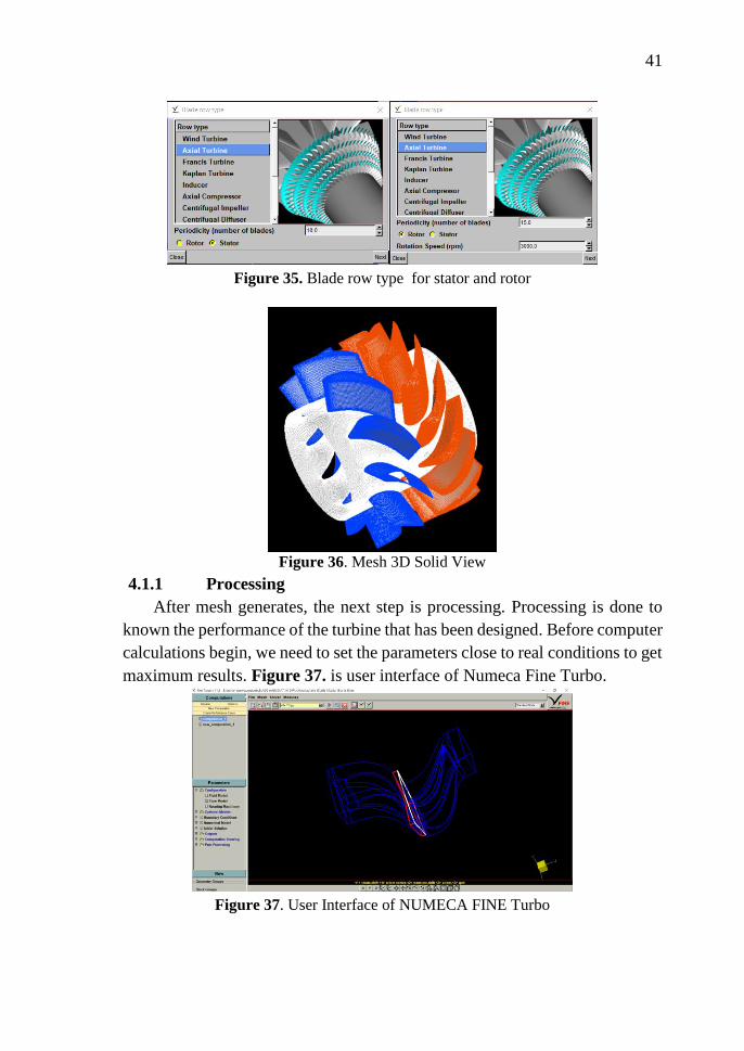
Figure 35. Blade row type for stator and rotor
Figure 36. Mesh 3D Solid View
4.1.1 Processing
After mesh generates, the next step is processing. Processing is done to
known the performance of the turbine that has been designed. Before computer
calculations begin, we need to set the parameters close to real conditions to get
maximum results. Figure 37. is user interface of Numeca Fine Turbo.
Figure 37. User Interface of NUMECA FINE Turbo

42
Figure After setting the parameters, then the calculation process by
computer based on the boundary condition, shown in Figure 38. Inlet, and
Figure 39. Outlet. All parameters can be seen on Attachment 3.
Figure 38. Boundary Condition Inlet
Figure 39. Boundary Condition Outlet
The iteration process is carried out until converge condition, mass flow
in and out are in balanced condition. Mass flow graphic can be seen on Figure
40. efficiency graphic can be seen on Figure 41. Torque graphic can be seen
on Figure 42. After reaching convergence conditions the results are
summarized on the convergence history tab which can be seen on the Figure
43. Torque used to calculate power generated by OTEC Turbine. Mass flow
used to calculate the warm and cold seawater requirement on evaporator and
condenser.

43
Figure 40. Mass Flow Graphic
Figure 41. Efficiency Graphic
44
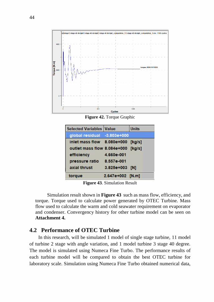
Figure 42. Torque Graphic
Figure 43. Simulation Result
Simulation result shown in Figure 43 such as mass flow, efficiency, and
torque. Torque used to calculate power generated by OTEC Turbine. Mass
flow used to calculate the warm and cold seawater requirement on evaporator
and condenser. Convergency history for other turbine model can be seen on
Attachment 4.
4.2 Performance of OTEC Turbine
In this research, will be simulated 1 model of single stage turbine, 11 model
of turbine 2 stage with angle variation, and 1 model turbine 3 stage 40 degree.
The model is simulated using Numeca Fine Turbo. The performance results of
each turbine model will be compared to obtain the best OTEC turbine for
laboratory scale. Simulation using Numeca Fine Turbo obtained numerical data,
45
such as mass flow balance (inlet and outlet), efficiency, and torque shown in
Table 5. Torque used to calculate power generated by OTEC Turbine. Mass flow
used to calculate the warm and cold seawater needs on evaporator and condenser.
Table 5. Result of OTEC’s Turbine Simulation
No. Name RPM Mass Flow
In (kg/s)
Mass
Flow Out
(kg/s)
Efficiency
(%) Torque
1 Single Stage 3000 8,291 8,294 45,85 288,8
2 2 Stage 0 Degree 3000 6,17 6,175 41,17 316,9
3 2 Stage 5 Degree 3000 8,21 8,19 42,3 500
4 2 Stage 10 Degree 3000 8,9 8,898 46,75 620,58
5 2 Stage 15 Degree 3000 12,37 12,38 45,33 958
6 2 Stage 20 Degree 3000 12,97 13,02 55,05 1177
7 2 Stage 25 Degree 3000 14,52 14,56 55,04 1396
8 2 Stage 30 Degree 3000 15,83 15,85 53,97 1584
9 2 Stage 35 Degree 3000 16,8 16,82 54,89 1744
10 2 Stage 40 Degree 3000 17,86 17,94 57,45 1943
11 2 Stage 45 Degree 3000 17,77 17,82 53,89 1852
12 2 Stage 50 Degree 3000 17,32 17,35 49,87 1632
13 3 Stage 40 Degree 3000 17,42 17,57 65,02 2084
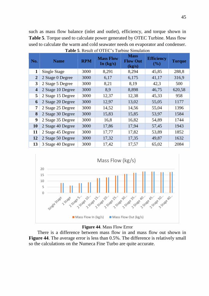
Figure 44. Mass Flow Error
There is a difference between mass flow in and mass flow out shown in
Figure 44. The average error is less than 0.5%. The difference is relatively small
so the calculations on the Numeca Fine Turbo are quite accurate.
0
5
10
15
20
Mass Flow (kg/s)
Mass Flow In (kg/s) Mass Flow Out (kg/s)

46
Figure 45. Efficiency of OTEC’s Turbine
Figure 45 shown the efficiency from each model that has been simulated
using Numeca Fine Turbo. Single stage turbine has an efficiency of 45.85%. For
2 stage turbine, the lowest efficiency is a straight turbine with the efficiency of
41.17%, and the highest efficiency is 2 stage turbine 40 degree with the efficiency
of 57.45%. The 3 stage turbine has an efficiency of 65.02%. The author made a 3
stage turbine 40 degrees model in order to increase efficiency and power
generated.
4.2.1 Calculation of OTEC Turbine Power
The results of the simulation using Numeca Fine Turbo is the torque that
used to calculate the power generated by the OTEC turbine. The results of the
simulation can be seen in Table 5. To known the power generated by the turbine
can be calculated using the formula:
𝑃 = 𝑇 × 2𝜋 × 𝑅𝑃𝑀/60000
Below is an example of turbine power calculation for a single stage turbine
based on Table. In the same way, the result of turbine power shown in Table 6.
𝑃 = 𝑇 × 2𝜋 × 𝑅𝑃𝑀/60000
𝑃 = 288.8 × 2 (22
7) ×
3000
60000
𝑃 = 90.77 𝑘𝑊
Table 6. Calculation of Turbine Power
010203040506070
Efficiency
Efficiency (%)

47
No. Name RPM Torque
(Nm)
Power
(kW)
1 Single Stage 3000 288,8 90,77
2 2 Stage 3000 316,9 99,60
3 2 Stage 5 Degree 3000 500 157,14
4 2 Stage 10 Degree 3000 620,58 195,04
5 2 Stage 15 Degree 3000 958 301,09
6 2 Stage 20 Degree 3000 1177 369,91
7 2 Stage 25 Degree 3000 1396 438,74
8 2 Stage 30 Degree 3000 1584 497,83
9 2 Stage 35 Degree 3000 1744 548,11
10 2 Stage 40 Degree 3000 1943 610,66
11 2 Stage 45 Degree 3000 1852 582,06
12 2 Stage 50 Degree 3000 1632 512,91
13 3 Stage 40 Degree 3000 2084 654,97
Figure 46. Efficiency of OTEC’s Turbine
From Figure 46 can be seen the power generated from each model that has
been simulated using Numeca Fine Turbo. The single stage turbine produces
90.77 kW. Meanwhile, for the 2 stage turbine, the lowest is a straight turbine
that produces 99.60 kW, and the highest is a turbine with 40 degree of slope that
produces 610.66 kW. The author made a 3 stage turbine 40 degrees model in
0
100
200
300
400
500
600
700
Power (kW)

48
order to increase efficiency and power generated which is have 65.02% of
efficiency, and produce 654.97 kW.
4.2.2 Calculation of Volume Flow Rate
In order for an Ocean Thermal Energy Conversion (OTEC) system to
work, it needs ammonia as a working fluid, warm seawater used to change the
ammonia phase from liquid to vapor, and cold seawater used to change the vapor
phase to liquid. In this section will explain how to calculate the volume flow rate
of ammonia, warm seawater, and cold seawater.
1. Calculation of Ammonia Volume Rate
In the Ocean Thermal Energy Conversion (OTEC) system, ammonia is
used as a working fluid that will rotate the turbine so that the turbine can
generate power. simulation results in Table 6 has been known mass flow
of ammonia. The following is an example of calculating of ammonia
volume flow rate needs on a single stage turbine:
𝑉𝑜𝑙𝑢𝑚𝑒 𝐹𝑙𝑜𝑤 𝑅𝑎𝑡𝑒 (𝑄) = ṁ × 𝑣
𝑉𝑜𝑙𝑢𝑚𝑒 𝐹𝑙𝑜𝑤 𝑅𝑎𝑡𝑒 (𝑄) = 8.297 𝑘𝑔/𝑠 × 1.6008 × 10⁻³𝑚3/𝑘𝑔
𝑉𝑜𝑙𝑢𝑚𝑒 𝐹𝑙𝑜𝑤 𝑅𝑎𝑡𝑒 (𝑄) = 0.0013 𝑚3/𝑠
𝑉𝑜𝑙𝑢𝑚𝑒 𝐹𝑙𝑜𝑤 𝑅𝑎𝑡𝑒 (𝑄) = 47.78 𝑚3/ℎ
By using the same step, the result of ammonia volume flow rate can be
seen in Table 7.
Table 7. Result of Ammonia Volume Flow Rate Calculation
No. Name
Mass
Flow In
(kg/s)
Volume Flow
Rate
m3/s (m3/h)
1 Single Stage 8,291 0,0133 47,78
2 2 Stage 6,17 0,0099 35,56
3 2 Stage 5 Degree 8,21 0,0131 47,31
4 2 Stage 10 Degree 8,9 0,0142 51,29
5 2 Stage 15 Degree 12,37 0,0198 71,29
6 2 Stage 20 Degree 12,97 0,0208 74,74
7 2 Stage 25 Degree 14,52 0,0232 83,68
8 2 Stage 30 Degree 15,83 0,0253 91,23
9 2 Stage 35 Degree 16,8 0,0269 96,82
10 2 Stage 40 Degree 17,86 0,0286 102,93
11 2 Stage 45 Degree 17,77 0,0284 102,41
49
12 2 Stage 50 Degree 17,32 0,0277 99,81
13 3 Stage 40 Degree 17,42 0,0279 100,39
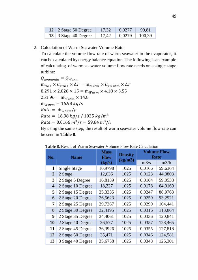
2. Calculation of Warm Seawater Volume Rate
To calculate the volume flow rate of warm seawater in the evaporator, it
can be calculated by energy balance equation. The following is an example
of calculating of warm seawater volume flow rate needs on a single stage
turbine:
𝑄𝑎𝑚𝑚𝑜𝑛𝑖𝑎 = 𝑄𝑊𝑎𝑟𝑚
ṁ𝑁𝐻3 × 𝐶𝑝𝑁𝐻3 × ∆𝑇 = ṁ𝑊𝑎𝑟𝑚 × 𝐶𝑝𝑊𝑎𝑟𝑚 × ∆𝑇
8.291 × 2.026 × 15 = ṁ𝑊𝑎𝑟𝑚 × 4.18 × 3.55
251.96 = ṁ𝑊𝑎𝑟𝑚 × 14.8
ṁ𝑊𝑎𝑟𝑚 = 16.98 𝑘𝑔/𝑠
𝑅𝑎𝑡𝑒 = ṁ𝑊𝑎𝑟𝑚/𝜌
𝑅𝑎𝑡𝑒 = 16.98 𝑘𝑔/𝑠 / 1025 𝑘𝑔/𝑚3
𝑅𝑎𝑡𝑒 = 0.0166 𝑚3/𝑠 = 59.64 𝑚3/ℎ
By using the same step, the result of warm seawater volume flow rate can
be seen in Table 8.
Table 8. Result of Warm Seawater Volume Flow Rate Calculation
No. Name
Mass
Flow
(kg/s)
Density
(kg/m3)
Volume Flow
Rate
m3/s m3/h
1 Single Stage 16,9798 1025 0,0166 59,6364
2 2 Stage 12,636 1025 0,0123 44,3803
3 2 Stage 5 Degree 16,8139 1025 0,0164 59,0538
4 2 Stage 10 Degree 18,227 1025 0,0178 64,0169
5 2 Stage 15 Degree 25,3335 1025 0,0247 88,9763
6 2 Stage 20 Degree 26,5623 1025 0,0259 93,2921
7 2 Stage 25 Degree 29,7367 1025 0,0290 104,441
8 2 Stage 30 Degree 32,4195 1025 0,0316 113,864
9 2 Stage 35 Degree 34,4061 1025 0,0336 120,841
10 2 Stage 40 Degree 36,577 1025 0,0357 128,465
11 2 Stage 45 Degree 36,3926 1025 0,0355 127,818
12 2 Stage 50 Degree 35,471 1025 0,0346 124,581
13 3 Stage 40 Degree 35,6758 1025 0,0348 125,301

50
3. Calculation of Cold Seawater Volume Rate
To calculate the volume flow rate of cold seawater in the condenser, it can
be calculated by energy balance equation. The following is an example of
calculating of cold seawater volume flow rate needs on a single stage
turbine:
𝑄𝑎𝑚𝑚𝑜𝑛𝑖𝑎 = 𝑄𝐶𝑜𝑙𝑑
ṁ𝑁𝐻3 × 𝐶𝑝𝑁𝐻3 × ∆𝑇 = ṁ𝐶𝑜𝑙𝑑 × 𝐶𝑝𝐶𝑜𝑙𝑑 × ∆𝑇
8.291 × 4.676 × 1 = ṁ𝐶𝑜𝑙𝑑 × 3.987 × 2
38.77 = ṁ𝐶𝑜𝑙𝑑 × 7.947
ṁ𝐶𝑜𝑙𝑑 = 4.86 𝑘𝑔/𝑠
𝑅𝑎𝑡𝑒 = ṁ𝑁𝐻3/𝜌
𝑅𝑎𝑡𝑒 = 4.86 𝑘𝑔/𝑠 / 1025 𝑘𝑔/𝑚3
𝑅𝑎𝑡𝑒 = 0.0047 𝑚3/𝑠 = 17.08 𝑚3/ℎ
By using the same step, the result of warm seawater volume flow rate can
be seen in Table 9.
Table 9. Result of Cold Seawater Volume Flow Rate Calculation
No. Name
Mass
Flow
(kg/s)
Density
(kg/m3)
Volume Flow
Rate
m3/s m3/h
1 Single Stage 4,86 1025 0,0047 17,08
2 2 Stage 3,62 1025 0,0035 12,71
3 2 Stage 5 Degree 4,81 1025 0,0047 16,91
4 2 Stage 10 Degree 5,22 1025 0,0051 18,33
5 2 Stage 15 Degree 7,25 1025 0,0071 25,48
6 2 Stage 20 Degree 7,61 1025 0,0074 26,71
7 2 Stage 25 Degree 8,51 1025 0,0083 29,90
8 2 Stage 30 Degree 9,28 1025 0,0091 32,60
9 2 Stage 35 Degree 9,85 1025 0,0096 34,60
10 2 Stage 40 Degree 10,47 1025 0,0102 36,78
11 2 Stage 45 Degree 10,42 1025 0,0102 36,60
12 2 Stage 50 Degree 10,16 1025 0,0099 35,67
13 3 Stage 40 Degree 10,22 1025 0,0100 35,84

51
4.2.3 Calculation of Heat Exchanger
The ocean thermal energy conversion (OTEC) system requires
evaporators and condenser. An evaporator used to turn the liquid form of a
chemical substance such as water into its gaseous-form/vapor. A condenser
used to condense a substance from its gaseous to its liquid state, by cooling
it. In this section will explain the calculation of the surface area and the
number of tubes required for the evaporator and condenser.
1. Evaporator
Figure 47. Evaporator
Figure 47 shown the Evaporator. In the evaporator, there is a
difference of sea water temperature at inlet = 28°C and outlet = 24.45°C.
In this research using tube and shell heat exchangers. Calculation using
LMTD method. Below is an example calculation for evaporator on single
stage turbine.
• Calculation of LMTD
𝐿𝑀𝑇𝐷 =(𝑇𝑤𝑎𝑟𝑚,𝑖𝑛 − 𝑇𝑁𝐻3,𝑜𝑢𝑡) − (𝑇𝑤𝑎𝑟𝑚,𝑜𝑢𝑡 − 𝑇𝑁𝐻3,𝑖𝑛)
ln [ (𝑇𝑤𝑎𝑟𝑚,𝑖𝑛 − 𝑇𝑁𝐻3,𝑜𝑢𝑡)(𝑇𝑤𝑎𝑟𝑚,𝑜𝑢𝑡 − 𝑇𝑁𝐻3,𝑖𝑛)
]
𝐿𝑀𝑇𝐷 =(28°𝐶 − 24°𝐶) − (24.5°𝐶 − 9°𝐶)
ln [ (28°𝐶 − 24°𝐶)(24.5°𝐶 − 9°𝐶)
]
𝐿𝑀𝑇𝐷 = 8.47
• LMTD Correction Factor (F)
For shell and tube heat exchange cross-flow that having more than
one or more multi flow passes, whether in shell or tube arrangement,
in this case the LMTD values obtained must be corrected by
correction factor (F). LMTD correction factor can be found by using
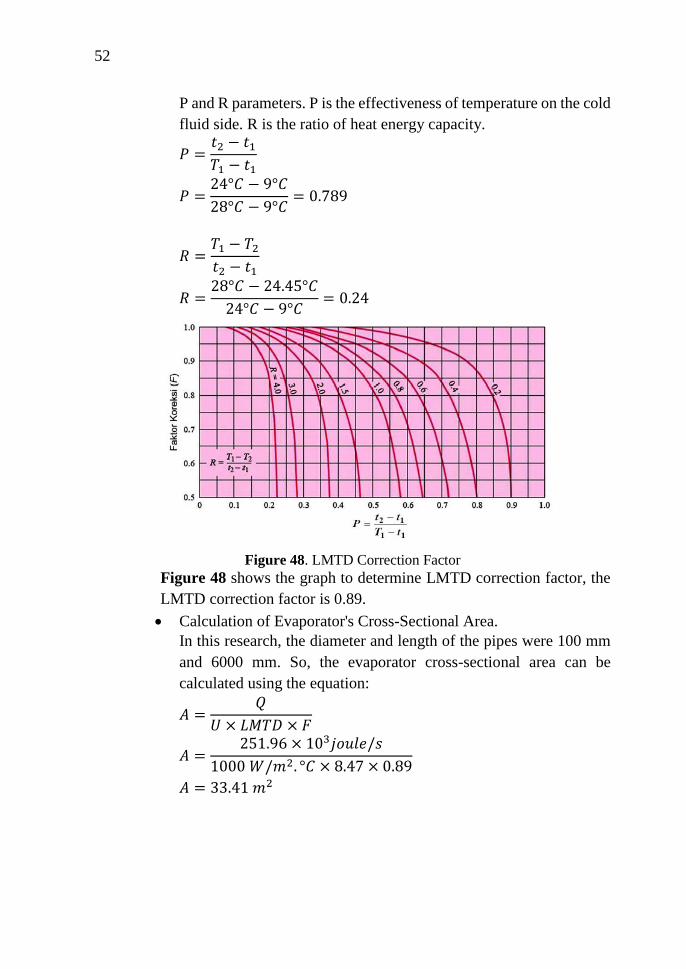
52
P and R parameters. P is the effectiveness of temperature on the cold
fluid side. R is the ratio of heat energy capacity.
𝑃 =𝑡2 − 𝑡1
𝑇1 − 𝑡1
𝑃 =24°𝐶 − 9°𝐶
28°𝐶 − 9°𝐶= 0.789
𝑅 =𝑇1 − 𝑇2
𝑡2 − 𝑡1
𝑅 =28°𝐶 − 24.45°𝐶
24°𝐶 − 9°𝐶= 0.24
Figure 48. LMTD Correction Factor
Figure 48 shows the graph to determine LMTD correction factor, the
LMTD correction factor is 0.89.
• Calculation of Evaporator's Cross-Sectional Area.
In this research, the diameter and length of the pipes were 100 mm
and 6000 mm. So, the evaporator cross-sectional area can be
calculated using the equation:
𝐴 =𝑄
𝑈 × 𝐿𝑀𝑇𝐷 × 𝐹
𝐴 =251.96 × 10³𝑗𝑜𝑢𝑙𝑒/𝑠
1000 𝑊/𝑚2. °𝐶 × 8.47 × 0.89
𝐴 = 33.41 𝑚2
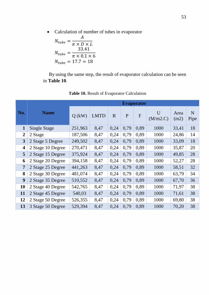
53
• Calculation of number of tubes in evaporator
𝑁𝑡𝑢𝑏𝑒 =𝐴
𝜋 × 𝐷 × 𝐿
𝑁𝑡𝑢𝑏𝑒 =33.41
𝜋 × 0.1 × 6
𝑁𝑡𝑢𝑏𝑒 = 17.7 = 18
By using the same step, the result of evaporator calculation can be seen
in Table 10.
Table 10. Result of Evaporator Calculation
No. Name
Evaporator
Q (kW) LMTD R P F U
(M/m2.C)
Area
(m2)
N
Pipe
1 Single Stage 251,963 8,47 0,24 0,79 0,89 1000 33,41 18
2 2 Stage 187,506 8,47 0,24 0,79 0,89 1000 24,86 14
3 2 Stage 5 Degree 249,502 8,47 0,24 0,79 0,89 1000 33,09 18
4 2 Stage 10 Degree 270,471 8,47 0,24 0,79 0,89 1000 35,87 20
5 2 Stage 15 Degree 375,924 8,47 0,24 0,79 0,89 1000 49,85 28
6 2 Stage 20 Degree 394,158 8,47 0,24 0,79 0,89 1000 52,27 28
7 2 Stage 25 Degree 441,263 8,47 0,24 0,79 0,89 1000 58,51 32
8 2 Stage 30 Degree 481,074 8,47 0,24 0,79 0,89 1000 63,79 34
9 2 Stage 35 Degree 510,552 8,47 0,24 0,79 0,89 1000 67,70 36
10 2 Stage 40 Degree 542,765 8,47 0,24 0,79 0,89 1000 71,97 38
11 2 Stage 45 Degree 540,03 8,47 0,24 0,79 0,89 1000 71,61 38
12 2 Stage 50 Degree 526,355 8,47 0,24 0,79 0,89 1000 69,80 38
13 3 Stage 50 Degree 529,394 8,47 0,24 0,79 0,89 1000 70,20 38

54
2. Condensor
Figure 49. Condenser
Figure 49 shown the Condenser. In the condenser, there is a
difference temperature of cold seawater temperature at inlet = 6°C and
outlet = 8°C. In this research using tube and shell heat exchangers.
Calculation using LMTD method. Below is an example calculation for
condes on single stage turbine.
• Calculation of LMTD
𝐿𝑀𝑇𝐷 =(𝑇𝑤𝑎𝑟𝑚,𝑖𝑛 − 𝑇𝑁𝐻3,𝑜𝑢𝑡) − (𝑇𝑤𝑎𝑟𝑚,𝑜𝑢𝑡 − 𝑇𝑁𝐻3,𝑖𝑛)
ln [ (𝑇𝑤𝑎𝑟𝑚,𝑖𝑛 − 𝑇𝑁𝐻3,𝑜𝑢𝑡)(𝑇𝑤𝑎𝑟𝑚,𝑜𝑢𝑡 − 𝑇𝑁𝐻3,𝑖𝑛)
]
𝐿𝑀𝑇𝐷 =(10°𝐶 − 8°𝐶) − (9°𝐶 − 6°𝐶)
ln [ (10°𝐶 − 8°𝐶)(9°𝐶 − 6°𝐶)
]
𝐿𝑀𝑇𝐷 = 2.47
• LMTD Correction Factor (F)
For shell and tube heat exchange cross-flow that having more than
one or more multi flow passes, whether in shell or tube arrangement,
in this case the LMTD values obtained must be corrected by
correction factor (F). LMTD correction factor can be found by using
P and R parameters. P is the effectiveness of temperature on the cold
fluid side. R is the ratio of heat energy capacity.
𝑃 =𝑡2 − 𝑡1
𝑇1 − 𝑡1
𝑃 =9°𝐶 − 10°𝐶
6°𝐶 − 10°𝐶= 0.25

55
𝑅 =𝑇1 − 𝑇2
𝑡2 − 𝑡1
𝑅 =6°𝐶 − 8°𝐶
9°𝐶 − 10°𝐶= 2
Figure 50. LMTD Correction Factor
Figure 50 shows the graph to determine LMTD correction factor,
the LMTD correction factor is 0.89.
• Calculation of Evaporator's Cross-Sectional Area.
In this research, the diameter and length of the pipes were 100 mm
and 6000 mm. So, the evaporator cross-sectional area can be
calculated using the equation:
𝐴 =𝑄
𝑈 × 𝐿𝑀𝑇𝐷 × 𝐹
𝐴 =38.77 × 10³𝑗𝑜𝑢𝑙𝑒/𝑠
1000 𝑊/𝑚2. °𝐶 × 2.47 × 0.89
𝐴 = 17.66 𝑚2
• Calculation of number of tube in evaporator
𝑁𝑡𝑢𝑏𝑒 =𝐴
𝜋 × 𝐷 × 𝐿
𝑁𝑡𝑢𝑏𝑒 =17.66
𝜋 × 0.1 × 6
𝑁𝑡𝑢𝑏𝑒 = 9.37 = 10

56
By using the same step, the result of evaporator calculation can be seen
in Table 11.
Table 11. Result of Condenser Calculation
No. Name
Condenser
Q
(kW) LMTD R P F
U
(M/m2.C)
Area
(m2)
N
Pipe
1 Single Stage 38,77 2,47 2,00 0,25 0,89 1000 17,66 10
2 2 Stage 28,85 2,47 2,00 0,25 0,89 1000 13,14 8
3 2 Stage 5 Degree 38,39 2,47 2,00 0,25 0,89 1000 17,49 10
4 2 Stage 10 Degree 41,62 2,47 2,00 0,25 0,89 1000 18,96 10
5 2 Stage 15 Degree 57,84 2,47 2,00 0,25 0,89 1000 26,35 14
6 2 Stage 20 Degree 60,65 2,47 2,00 0,25 0,89 1000 27,63 16
7 2 Stage 25 Degree 67,90 2,47 2,00 0,25 0,89 1000 30,93 18
8 2 Stage 30 Degree 74,02 2,47 2,00 0,25 0,89 1000 33,72 18
9 2 Stage 35 Degree 78,56 2,47 2,00 0,25 0,89 1000 35,79 20
10 2 Stage 40 Degree 83,51 2,47 2,00 0,25 0,89 1000 38,05 20
11 2 Stage 45 Degree 83,09 2,47 2,00 0,25 0,89 1000 37,86 20
12 2 Stage 50 Degree 80,99 2,47 2,00 0,25 0,89 1000 36,90 20
13 3 Stage 50 Degree 81,46 2,47 2,00 0,25 0,89 1000 37,11 20
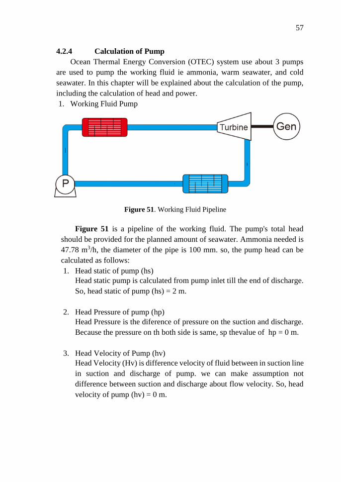
57
4.2.4 Calculation of Pump
Ocean Thermal Energy Conversion (OTEC) system use about 3 pumps
are used to pump the working fluid ie ammonia, warm seawater, and cold
seawater. In this chapter will be explained about the calculation of the pump,
including the calculation of head and power.
1. Working Fluid Pump
Figure 51. Working Fluid Pipeline
Figure 51 is a pipeline of the working fluid. The pump's total head
should be provided for the planned amount of seawater. Ammonia needed is
47.78 m3/h, the diameter of the pipe is 100 mm. so, the pump head can be
calculated as follows:
1. Head static of pump (hs)
Head static pump is calculated from pump inlet till the end of discharge.
So, head static of pump (hs) = 2 m.
2. Head Pressure of pump (hp)
Head Pressure is the diference of pressure on the suction and discharge.
Because the pressure on th both side is same, sp thevalue of hp = 0 m.
3. Head Velocity of Pump (hv)
Head Velocity (Hv) is difference velocity of fluid between in suction line
in suction and discharge of pump. we can make assumption not
difference between suction and discharge about flow velocity. So, head
velocity of pump (hv) = 0 m.

58
4. Head Loss
Head losses are the sum of head major and minor on both of suction and
discharge. Head Losses including head major and head minor in suction
and discharge. Below is calculation example of single stage turbine.
4.1. Calculation of Suction Head
• Major Head Losses
𝑅𝑒𝑦𝑛𝑜𝑙𝑑 𝑛𝑢𝑚𝑏𝑒𝑟 (𝑅𝑛) =𝑣 × 𝑑
𝜇
𝑅𝑒𝑦𝑛𝑜𝑙𝑑 𝑛𝑢𝑚𝑏𝑒𝑟 (𝑅𝑛) =0.024 × 0.1
0.00000098= 6925.7
Where: v = flow velocity ( 0.024 m/s)
d = inner diameter of pipe (0.1m)
μ = kinematis viscosity (9.8 x 10⁻⁷ m2/s)
If Re>2300 = Turbulen
If Re<2300 = Laminer
Because of turbulen flow, so the equation
𝑓 = 0.02 + 0.0005/𝑑
𝑓 = 0.025
𝑀𝑎𝑗𝑜𝑟 𝑙𝑜𝑠𝑠𝑒𝑠 =𝑓 × 𝐿 × 𝑣2
𝑑 × 2𝑔
Where:
L = Length of suction pipe = 60 m (estimation)
G = Gravitation = 9.8 m2/s
D = inner diameter of pipe = 100 mm = 0.1 m
So, 𝑀𝑎𝑗𝑜𝑟 𝑙𝑜𝑠𝑠𝑒𝑠 =0.025×60×0.0672
0.1×2(9.8)= 0.0035 𝑚
• Minor Head Loss
No Accessories n k n x k
1 Elbow 90o 2 0,8 1,6
2 Strainer 2 2,5 5
3 Gate Valve 2 0,2 0,4
Ʃ nk 7
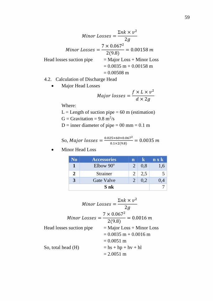
59
𝑀𝑖𝑛𝑜𝑟 𝐿𝑜𝑠𝑠𝑒𝑠 =Ʃ𝑛𝑘 × 𝑣2
2𝑔
𝑀𝑖𝑛𝑜𝑟 𝐿𝑜𝑠𝑠𝑒𝑠 =7 × 0.0672
2(9.8)= 0.00158 𝑚
Head losses suction pipe = Major Loss + Minor Loss
= 0.0035 m + 0.00158 m
= 0.00508 m
4.2. Calculation of Discharge Head
• Major Head Losses
𝑀𝑎𝑗𝑜𝑟 𝑙𝑜𝑠𝑠𝑒𝑠 =𝑓 × 𝐿 × 𝑣2
𝑑 × 2𝑔
Where:
L = Length of suction pipe = 60 m (estimation)
G = Gravitation = 9.8 m2/s
D = inner diameter of pipe = 00 mm = 0.1 m
So, 𝑀𝑎𝑗𝑜𝑟 𝑙𝑜𝑠𝑠𝑒𝑠 =0.025×60×0.0672
0.1×2(9.8)= 0.0035 𝑚
• Minor Head Loss
No Accessories n k n x k
1 Elbow 90o 2 0,8 1,6
2 Strainer 2 2,5 5
3 Gate Valve 2 0,2 0,4
S nk 7
𝑀𝑖𝑛𝑜𝑟 𝐿𝑜𝑠𝑠𝑒𝑠 =Ʃ𝑛𝑘 × 𝑣2
2𝑔
𝑀𝑖𝑛𝑜𝑟 𝐿𝑜𝑠𝑠𝑒𝑠 =7 × 0.0672
2(9.8)= 0.0016 𝑚
Head losses suction pipe = Major Loss + Minor Loss
= 0.0035 m + 0.0016 m
= 0.0051 m
So, total head (H) = hs + hp + hv + hl
= 2.0051 m
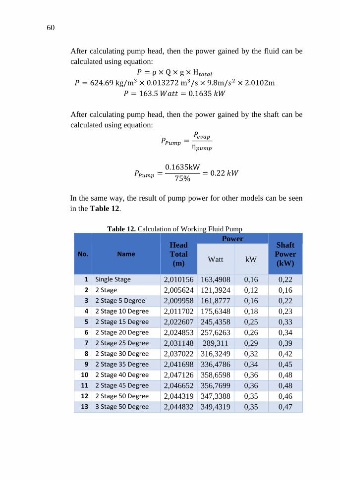
60
After calculating pump head, then the power gained by the fluid can be
calculated using equation:
𝑃 = ρ × Q × g × H𝑡𝑜𝑡𝑎𝑙
𝑃 = 624.69 kg/m3 × 0.013272 m3/s × 9.8m/𝑠2 × 2.0102m
𝑃 = 163.5 𝑊𝑎𝑡𝑡 = 0.1635 𝑘𝑊
After calculating pump head, then the power gained by the shaft can be
calculated using equation:
𝑃𝑃𝑢𝑚𝑝 =𝑃𝑒𝑣𝑎𝑝
η𝑝𝑢𝑚𝑝
𝑃𝑃𝑢𝑚𝑝 =0.1635kW
75%= 0.22 𝑘𝑊
In the same way, the result of pump power for other models can be seen
in the Table 12.
Table 12. Calculation of Working Fluid Pump
No. Name Head
Total
(m)
Power Shaft
Power
(kW) Watt kW
1 Single Stage 2,010156 163,4908 0,16 0,22
2 2 Stage 2,005624 121,3924 0,12 0,16
3 2 Stage 5 Degree 2,009958 161,8777 0,16 0,22
4 2 Stage 10 Degree 2,011702 175,6348 0,18 0,23
5 2 Stage 15 Degree 2,022607 245,4358 0,25 0,33
6 2 Stage 20 Degree 2,024853 257,6263 0,26 0,34
7 2 Stage 25 Degree 2,031148 289,311 0,29 0,39
8 2 Stage 30 Degree 2,037022 316,3249 0,32 0,42
9 2 Stage 35 Degree 2,041698 336,4786 0,34 0,45
10 2 Stage 40 Degree 2,047126 358,6598 0,36 0,48
11 2 Stage 45 Degree 2,046652 356,7699 0,36 0,48
12 2 Stage 50 Degree 2,044319 347,3388 0,35 0,46
13 3 Stage 50 Degree 2,044832 349,4319 0,35 0,47
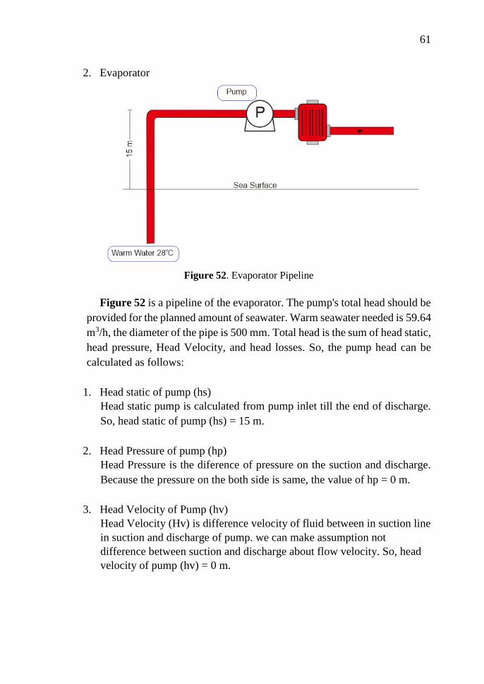
61
2. Evaporator
Figure 52. Evaporator Pipeline
Figure 52 is a pipeline of the evaporator. The pump's total head should be
provided for the planned amount of seawater. Warm seawater needed is 59.64
m3/h, the diameter of the pipe is 500 mm. Total head is the sum of head static,
head pressure, Head Velocity, and head losses. So, the pump head can be
calculated as follows:
1. Head static of pump (hs)
Head static pump is calculated from pump inlet till the end of discharge.
So, head static of pump (hs) = 15 m.
2. Head Pressure of pump (hp)
Head Pressure is the diference of pressure on the suction and discharge.
Because the pressure on the both side is same, the value of hp = 0 m.
3. Head Velocity of Pump (hv)
Head Velocity (Hv) is difference velocity of fluid between in suction line
in suction and discharge of pump. we can make assumption not
difference between suction and discharge about flow velocity. So, head
velocity of pump (hv) = 0 m.
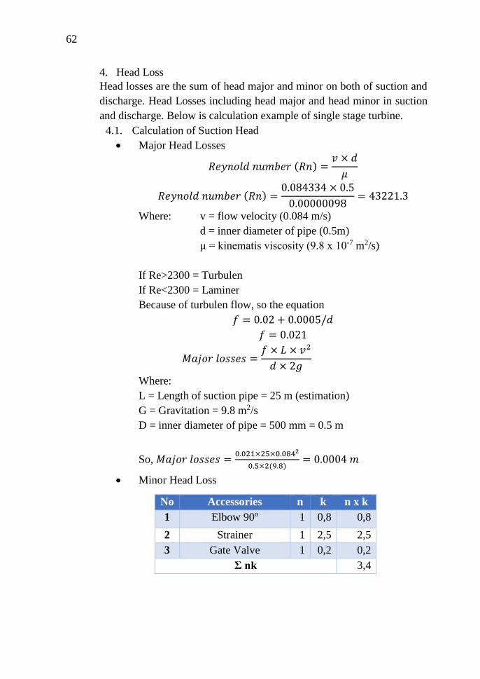
62
4. Head Loss
Head losses are the sum of head major and minor on both of suction and
discharge. Head Losses including head major and head minor in suction
and discharge. Below is calculation example of single stage turbine.
4.1. Calculation of Suction Head
• Major Head Losses
𝑅𝑒𝑦𝑛𝑜𝑙𝑑 𝑛𝑢𝑚𝑏𝑒𝑟 (𝑅𝑛) =𝑣 × 𝑑
𝜇
𝑅𝑒𝑦𝑛𝑜𝑙𝑑 𝑛𝑢𝑚𝑏𝑒𝑟 (𝑅𝑛) =0.084334 × 0.5
0.00000098= 43221.3
Where: v = flow velocity (0.084 m/s)
d = inner diameter of pipe (0.5m)
μ = kinematis viscosity (9.8 x 10⁻⁷ m2/s)
If Re>2300 = Turbulen
If Re<2300 = Laminer
Because of turbulen flow, so the equation
𝑓 = 0.02 + 0.0005/𝑑
𝑓 = 0.021
𝑀𝑎𝑗𝑜𝑟 𝑙𝑜𝑠𝑠𝑒𝑠 =𝑓 × 𝐿 × 𝑣2
𝑑 × 2𝑔
Where:
L = Length of suction pipe = 25 m (estimation)
G = Gravitation = 9.8 m2/s
D = inner diameter of pipe = 500 mm = 0.5 m
So, 𝑀𝑎𝑗𝑜𝑟 𝑙𝑜𝑠𝑠𝑒𝑠 =0.021×25×0.0842
0.5×2(9.8)= 0.0004 𝑚
• Minor Head Loss
No Accessories n k n x k
1 Elbow 90o 1 0,8 0,8
2 Strainer 1 2,5 2,5
3 Gate Valve 1 0,2 0,2
Ʃ nk 3,4

63
𝑀𝑖𝑛𝑜𝑟 𝐿𝑜𝑠𝑠𝑒𝑠 =Ʃ𝑛𝑘 × 𝑣2
2𝑔
𝑀𝑖𝑛𝑜𝑟 𝐿𝑜𝑠𝑠𝑒𝑠 =3.4 × 0.0842
2(9.8)= 0.0012 𝑚
Head losses suction pipe = Major Loss + Minor Loss
= 0.0004 m + 0.0012 m
= 0.00016 m
b. Calculation of Discharge Head
• Major Head Losses
𝑀𝑎𝑗𝑜𝑟 𝑙𝑜𝑠𝑠𝑒𝑠 =𝑓 × 𝐿 × 𝑣2
𝑑 × 2𝑔
Where:
L = Length of suction pipe = 15 m (estimation)
G = Gravitation = 9.8 m2/s
D = inner diameter of pipe = 500 mm = 0.5 m
So, 𝑀𝑎𝑗𝑜𝑟 𝑙𝑜𝑠𝑠𝑒𝑠 =0.021×15×0.0842
0.5×2(9.8)= 0.00023 𝑚
• Minor Head Loss
No Accessories n k n x k
1 Elbow 90o 1 0,8 0,8
2 Strainer 1 2,5 2,5
3 Gate Valve 1 0,2 0,2
S nk 3,4
𝑀𝑖𝑛𝑜𝑟 𝐿𝑜𝑠𝑠𝑒𝑠 =Ʃ𝑛𝑘 × 𝑣2
2𝑔
𝑀𝑖𝑛𝑜𝑟 𝐿𝑜𝑠𝑠𝑒𝑠 =3.4 × 0.0842
2(9.8)= 0.0012 𝑚
Head losses suction pipe = Major Loss + Minor Loss
= 0.00023 m + 0.00123 m
= 0.00146 m
So, total head (H) = hs + hp + hv + hl
= 15.0031 m
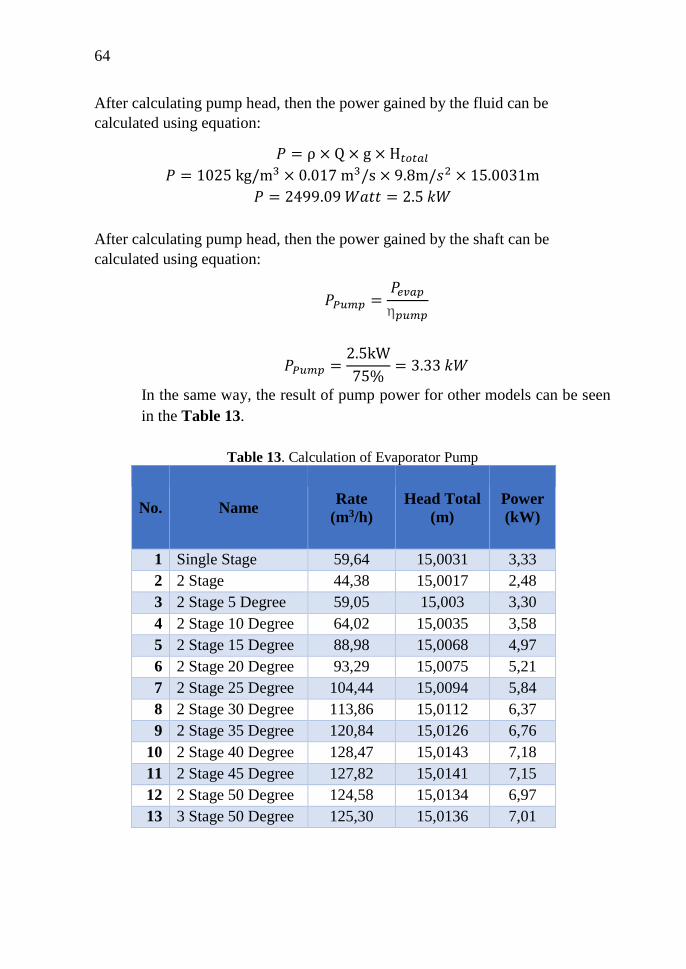
64
After calculating pump head, then the power gained by the fluid can be
calculated using equation:
𝑃 = ρ × Q × g × H𝑡𝑜𝑡𝑎𝑙
𝑃 = 1025 kg/m3 × 0.017 m3/s × 9.8m/𝑠2 × 15.0031m
𝑃 = 2499.09 𝑊𝑎𝑡𝑡 = 2.5 𝑘𝑊
After calculating pump head, then the power gained by the shaft can be
calculated using equation:
𝑃𝑃𝑢𝑚𝑝 =𝑃𝑒𝑣𝑎𝑝
η𝑝𝑢𝑚𝑝
𝑃𝑃𝑢𝑚𝑝 =2.5kW
75%= 3.33 𝑘𝑊
In the same way, the result of pump power for other models can be seen
in the Table 13.
Table 13. Calculation of Evaporator Pump
No. Name Rate
(m3/h)
Head Total
(m)
Power
(kW)
1 Single Stage 59,64 15,0031 3,33
2 2 Stage 44,38 15,0017 2,48
3 2 Stage 5 Degree 59,05 15,003 3,30
4 2 Stage 10 Degree 64,02 15,0035 3,58
5 2 Stage 15 Degree 88,98 15,0068 4,97
6 2 Stage 20 Degree 93,29 15,0075 5,21
7 2 Stage 25 Degree 104,44 15,0094 5,84
8 2 Stage 30 Degree 113,86 15,0112 6,37
9 2 Stage 35 Degree 120,84 15,0126 6,76
10 2 Stage 40 Degree 128,47 15,0143 7,18
11 2 Stage 45 Degree 127,82 15,0141 7,15
12 2 Stage 50 Degree 124,58 15,0134 6,97
13 3 Stage 50 Degree 125,30 15,0136 7,01

65
5. Condenser
Figure 53. Condenser Pipeline
Figure 53 is a pipeline of the condenser. The pump's total head should be
provided for the planned amount of seawater. Cold seawater needed is 17.08
m3/h, the diameter of the pipe is 500 mm. Total head is the sum of head static,
head pressure, Head Velocity, and head losses. So, the pump head can be
calculated as follows:
1. Head static of pump (hs)
Head static pump is calculated from pump inlet till the end of discharge.
So, head static of pump (hs) = 15 m.
2. Head Pressure of pump (hp)
Head Pressure is the diference of pressure on the suction and discharge.
Because the pressure on th both side is same, sp thevalue of hp = 0 m.
3. Head Velocity of Pump (hv)
Head Velocity (Hv) is difference velocity of fluid between in suction line
in suction and discharge of pump. we can make assumption not difference
between suction and discharge about flow velocity. So, head velocity of
pump (hv) = 0 m.

66
4. Head Losses
Head losses are the sum of head major and minor on both of suction and
discharge. Head Losses including head major and head minor in suction
and discharge. Below is calculation example of single stage turbine.
4.1. Calculation of Suction Head
• Major Head Losses
𝑅𝑒𝑦𝑛𝑜𝑙𝑑 𝑛𝑢𝑚𝑏𝑒𝑟 (𝑅𝑛) =𝑣 × 𝑑
𝜇
𝑅𝑒𝑦𝑛𝑜𝑙𝑑 𝑛𝑢𝑚𝑏𝑒𝑟 (𝑅𝑛) =0.024 × 0.5
0.00000098= 12375.7
Where: v = flow velocity (0.024 m/s)
d = inner diameter of pipe (0.5m)
μ = kinematis viscosity (9.8 x 10⁻⁷ m2/s)
If Re>2300 = Turbulen
If Re<2300 = Laminer
Because of turbulen flow, so the equation
𝑓 = 0.02 + 0.0005/𝑑
𝑓 = 0.021
𝑀𝑎𝑗𝑜𝑟 𝑙𝑜𝑠𝑠𝑒𝑠 =𝑓 × 𝐿 × 𝑣2
𝑑 × 2𝑔
Where:
L = Length of suction pipe = 650 m (estimation)
G = Gravitation = 9.8 m2/s
D = inner diameter of pipe = 500 mm = 0.5 m
So, 𝑀𝑎𝑗𝑜𝑟 𝑙𝑜𝑠𝑠𝑒𝑠 =0.021×650×0.0242
0.5×2(9.8)= 0.0007 𝑚
• Minor Head Loss
No Accessories n k n x k
1 Elbow 90o 1 0,8 0,8
2 Strainer 1 2,5 2,5
3 Gate Valve 1 0,2 0,2
Ʃ nk 3,4

67
𝑀𝑖𝑛𝑜𝑟 𝐿𝑜𝑠𝑠𝑒𝑠 =Ʃ𝑛𝑘 × 𝑣2
2𝑔
𝑀𝑖𝑛𝑜𝑟 𝐿𝑜𝑠𝑠𝑒𝑠 =3.4 × 0.0242
2(9.8)= 0.0001 𝑚
Head losses suction pipe = Major Loss + Minor Loss
= 0.0007 m + 0.0001 m
= 0.0008 m
4.2. Calculation of Discharge Head
• Major Head Losses
𝑀𝑎𝑗𝑜𝑟 𝑙𝑜𝑠𝑠𝑒𝑠 =𝑓 × 𝐿 × 𝑣2
𝑑 × 2𝑔
Where:
L = Length of suction pipe = 15 m (estimation)
G = Gravitation = 9.8 m2/s
D = inner diameter of pipe = 500 mm = 0.5 m
So, 𝑀𝑎𝑗𝑜𝑟 𝑙𝑜𝑠𝑠𝑒𝑠 =0.021×15×0.0242
0.5×2(9.8)= 0.00001 𝑚
• Minor Head Loss
No Accessories n k n x k
1 Elbow 90o 1 0,8 0,8
2 Strainer 1 2,5 2,5
3 Gate Valve 1 0,2 0,2
S nk 3,4
𝑀𝑖𝑛𝑜𝑟 𝐿𝑜𝑠𝑠𝑒𝑠 =Ʃ𝑛𝑘 × 𝑣2
2𝑔
𝑀𝑖𝑛𝑜𝑟 𝐿𝑜𝑠𝑠𝑒𝑠 =3.4 × 0.0242
2(9.8)= 0.0001 𝑚
Head losses suction pipe = Major Loss + Minor Loss
= 0.00001 m + 0.0001 m
= 0.00011 m
So, total head (H) = hs + hp + hv + hl
= 15.001 m
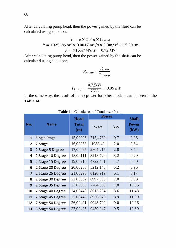
68
After calculating pump head, then the power gained by the fluid can be
calculated using equation:
𝑃 = ρ × Q × g × H𝑡𝑜𝑡𝑎𝑙
𝑃 = 1025 kg/m3 × 0.0047 m3/s × 9.8m/𝑠2 × 15.001m
𝑃 = 715.47 𝑊𝑎𝑡𝑡 = 0.72 𝑘𝑊
After calculating pump head, then the power gained by the shaft can be
calculated using equation:
𝑃𝑃𝑢𝑚𝑝 =𝑃𝑒𝑣𝑎𝑝
η𝑝𝑢𝑚𝑝
𝑃𝑃𝑢𝑚𝑝 =0.72kW
75%= 0.95 𝑘𝑊
In the same way, the result of pump power for other models can be seen in the
Table 14.
Table 14. Calculation of Condenser Pump
No. Name
Head
Total
(m)
Power Shaft
Power
(kW) Watt kW
1 Single Stage 15,00096 715,4732 0,7 0,95
2 2 Stage 16,00053 1983,42 2,0 2,64
3 2 Stage 5 Degree 17,00095 2804,215 2,8 3,74
4 2 Stage 10 Degree 18,00111 3218,729 3,2 4,29
5 2 Stage 15 Degree 19,00215 4722,451 4,7 6,30
6 2 Stage 20 Degree 20,00236 5212,143 5,2 6,95
7 2 Stage 25 Degree 21,00296 6126,919 6,1 8,17
8 2 Stage 30 Degree 22,00352 6997,905 7,0 9,33
9 2 Stage 35 Degree 23,00396 7764,383 7,8 10,35
10 2 Stage 40 Degree 24,00448 8613,284 8,6 11,48
11 2 Stage 45 Degree 25,00443 8926,875 8,9 11,90
12 2 Stage 50 Degree 26,00421 9048,709 9,0 12,06
13 3 Stage 50 Degree 27,00425 9450,947 9,5 12,60

69
4.2.5 Calculation of Nett Power
Nett power is the power that distributed to the consumer. Generator is
needed to generate power that will be distributed to the consumer. In this
research, generator efficiency is assumed to be 85%. Table 15. shown the power
generated by generator.
Table 15. Power generated by generator
No. Name Efficiency
(%)
Turbine Power
(kW) Generator (kW)
Simulation Nett Efficiency Power
1 Single Stage 45,85 90,77 41,62 85 35,37
2 2 Stage 41,17 99,60 41,00 85 34,85
3 2 Stage 5 Degree 42,3 157,14 66,47 85 56,50
4 2 Stage 10 Degree 46,75 195,04 91,18 85 77,50
5 2 Stage 15 Degree 45,33 301,09 136,48 85 116,01
6 2 Stage 20 Degree 55,05 369,91 203,64 85 173,09
7 2 Stage 25 Degree 55,04 438,74 241,48 85 205,26
8 2 Stage 30 Degree 53,97 497,83 268,68 85 228,38
9 2 Stage 35 Degree 54,89 548,11 300,86 85 255,73
10 2 Stage 40 Degree 57,45 610,66 350,82 85 298,20
11 2 Stage 45 Degree 53,89 582,06 313,67 85 266,62
12 2 Stage 50 Degree 49,87 512,91 255,79 85 217,42
13 3 Stage 40 Degree 65,02 654,97 425,86 85 361,98
After knowing the power generated by the generator, the pump calculation
needs to be done to know the nett power to be distributed to the consumer. Table
16. shown nett power to be delivered to the consumers.
Table 16. Nett Power
No. Name
Power by
Generator
(kW)
Pump Power (kW) Nett
Power
(kW) Evap Cond NH3
1 Single Stage 35,37 3,33 0,95 0,22 30,87
2 2 Stage 34,85 2,48 0,76 0,16 31,45
3 2 Stage 5 Degree 56,50 3,30 1,07 0,22 51,91
4 2 Stage 10 Degree 77,50 3,58 1,23 0,23 72,46
5 2 Stage 15 Degree 116,01 4,97 1,80 0,33 108,91
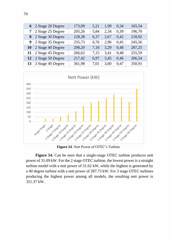
70
Figure 54. Nett Power of OTEC’s Turbine
Figure 54. Can be seen that a single-stage OTEC turbine produces nett
power of 31.09 kW. For the 2 stage OTEC turbine, the lowest power is a straight
turbine model with a nett power of 31.62 kW, while the highest is generated by
a 40 degree turbine with a nett power of 287.73 kW. For 3 stage OTEC turbines
producing the highest power among all models, the resulting nett power is
351.37 kW.
0
50
100
150
200
250
300
350
400
Nett Power (kW)
6 2 Stage 20 Degree 173,09 5,21 1,99 0,34 165,54
7 2 Stage 25 Degree 205,26 5,84 2,34 0,39 196,70
8 2 Stage 30 Degree 228,38 6,37 2,67 0,42 218,92
9 2 Stage 35 Degree 255,73 6,76 2,96 0,45 245,56
10 2 Stage 40 Degree 298,20 7,18 3,29 0,48 287,25
11 2 Stage 45 Degree 266,62 7,15 3,41 0,48 255,59
12 2 Stage 50 Degree 217,42 6,97 3,45 0,46 206,54
13 3 Stage 40 Degree 361,98 7,01 3,60 0,47 350,91
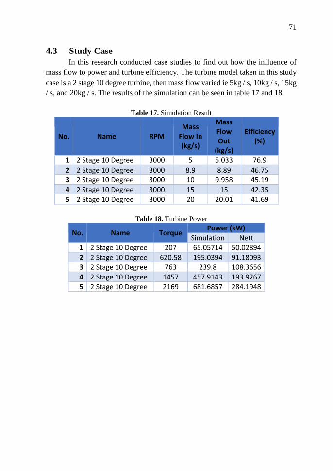
71
4.3 Study Case
In this research conducted case studies to find out how the influence of
mass flow to power and turbine efficiency. The turbine model taken in this study
case is a 2 stage 10 degree turbine, then mass flow varied ie 5kg / s, 10kg / s, 15kg
/ s, and 20kg / s. The results of the simulation can be seen in table 17 and 18.
Table 17. Simulation Result
No. Name RPM Mass
Flow In (kg/s)
Mass Flow Out
(kg/s)
Efficiency (%)
1 2 Stage 10 Degree 3000 5 5.033 76.9
2 2 Stage 10 Degree 3000 8.9 8.89 46.75
3 2 Stage 10 Degree 3000 10 9.958 45.19
4 2 Stage 10 Degree 3000 15 15 42.35
5 2 Stage 10 Degree 3000 20 20.01 41.69
Table 18. Turbine Power
No. Name Torque Power (kW)
Simulation Nett
1 2 Stage 10 Degree 207 65.05714 50.02894
2 2 Stage 10 Degree 620.58 195.0394 91.18093
3 2 Stage 10 Degree 763 239.8 108.3656
4 2 Stage 10 Degree 1457 457.9143 193.9267
5 2 Stage 10 Degree 2169 681.6857 284.1948

72
Figure 55. Mass Flow Vs Efficiency
From the graph in Figure 55 can be seen that 5kg / s mass flow has the highest
efficiency of 76.9%, while the lowest efficiency is mass flow 20 kg/s with the
efficiency of 41.69%.
Figure 56. Mass Flow Vs Torque
From the graph in Figure 55 can be seen that 5kg / s mass flow has the lowest
torque of 207 Nm, while the highest is mass flow 20 kg/s with the torque of 2169
Nm.
0
20
40
60
80
100
0 5 10 15 20 25
Per
cen
tage
(%
)
Mass Flow Rates
Mass Flow Vs Efficiency
0
500
1000
1500
2000
2500
0 5 10 15 20 25
Torq
ue
Mass Flow
Mass Flow Vs Torque

73
CHAPTER V
CONCLUSION
5.1 Conclusion
Based on the results of design and simulation that has been done, it can be
concluded as follows:
1. Design of the OTEC turbine conducted based on thermodynamic
conditions on a region. Turbine with Tin = 24 ° C, Pin = 9.7274 bar, and
Tout = 10 ° C, Pout = 6,1529 bar, have an enthalpy difference of 28.6 kJ /
kg using ammonia as working fluid. Result of calclation turbine blades
angle with α1 = 15° are: α2 = 31.78°, β1 = 24.1°, β2 = 21.1°.
2. The highest efficiency and net power is a 3 stage 40 degree turbine with
351.37 kW generated power, and 65.02% efficiency. Lowest is single
stage turbine with nett power 31.09 kW, and efficiency 45.85%.
5.2 Sugestion
1. Data collection in the field need to be done to get the result of research
approaching with real situation.
2. Further researches should be conducted about factors that affect the
performance of the OTEC turbine.
3. An experiment is needed to know the performance of OTEC turbines in
real terms.

74
“This page is intentionally left blank”

75
REFERENCES
Agency, E. P. (2015). Catalogue of CHP Technologies.
Arismunandar, W. (2004). Penggerak Mula Turbin. Penerbit ITB.
Avery, W. H., & Wu, C. (1995). Renewable Energy from the Ocean: A Guide
to OTEC. Ocean Engineering. https://doi.org/10.1016/0029-
8018(95)90035-7
CFD-Online. (n.d.). General CFD FAQ. Retrieved from https://www.cfd-
online.com/Wiki/General_CFD_FAQ
Dewan Energi Nasional. (2015). Outlook Energy Indonesia 2015.
Dietzel, F., & Sriyono, D. (1996). Turbin Pompa dan Kompresor. Penerbit
Erlangga.
Holman, J. (2010). Heat Transfer. New York: The McGraw-Hill Companies,
Inc.
Rajput, R. K. (2006). Power system engineering. LAXMI PUBLICATIONS.
Reynolds, W. C., & Perkins, H. C. (1989). Termodinamika Teknik. Surabaya:
Penerbit Erlangga.
Rubenstein, D. A., Yin, W., & Frame, M. D. (2012). Fundamentals of Fluid
Mechanics. Biofluid Mechanics. https://doi.org/10.1016/B978-0-12-
381383-1.00002-3
Shlyakhin, P. (1999). Turbin Uap (Steam Turbines): Teori dan Rancangan.
Penerbit Erlangga.
Soesilo, K. K. (2017). SIMULASI SISTEM PEMBANGKIT OTEC SIKLUS
TERTUTUP DENGAN VARIASI FLUIDA KERJA AMMONIA (NH3)
DAN REFRIGERANT (R-12, R-22, R-23, R-32, R134a)
MENGGUNAKAN CYCLE TEMPO.
Syamsuddin, M. L., Attamimi, A., Nugraha, A. P., Gibran, S., Afifah, A. Q.,
& Oriana, N. (2015). OTEC Potential in the Indonesian Seas. Energy
Procedia, 65, 215–222. https://doi.org/10.1016/j.egypro.2015.01.028

76
“This page is intentionally left blank”

77
ATTACHMENT

78
“This page is intentionally left blank”

79
Attachment 1.
Table Properties of Ammonia

80
“This page is intentionally left blank”

81
Table Properties of Ammonia
Figure 1. Table Properties of Ammonia

82
“This page is intentionally left blank”

83
Attachment 2.
OTEC Turbine Models

84
“This page is intentionally left blank”

85
OTEC Turbine Models
Figure Single Stage Turbine
Figure 2 Stage Turbine

86
Figure 3. 2 Stage 5 Degree Turbine
Figure 4. 2 Stage 10 Degree Turbine
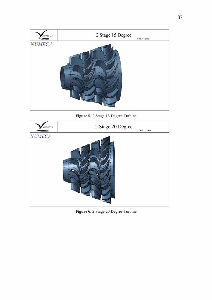
87
Figure 5. 2 Stage 15 Degree Turbine
Figure 6. 2 Stage 20 Degree Turbine
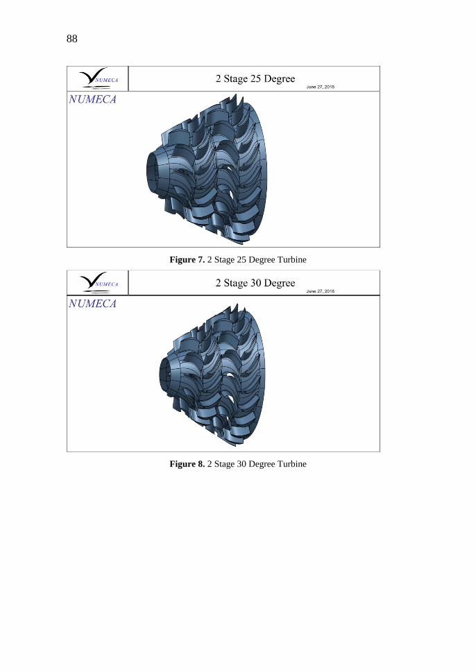
88
Figure 7. 2 Stage 25 Degree Turbine
Figure 8. 2 Stage 30 Degree Turbine

89
Figure 9. 2 Stage 35 Degree Turbine
Figure 10. 2 Stage 40 Degree Turbine

90
Figure 11. 2 Stage 45 Degree Turbine
Figure 12. 2 Stage 50 Degree Turbine
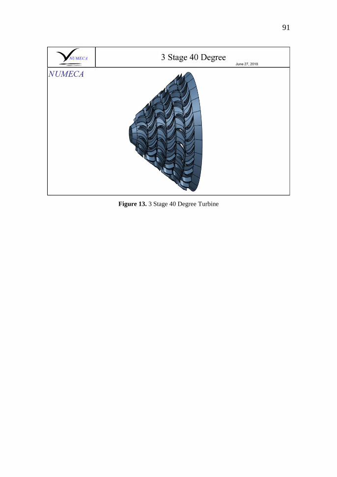
91
Figure 13. 3 Stage 40 Degree Turbine

92
“This page is intentionally left blank”

93
Attachment 3.
Simulation Parameter

94
“This page is intentionally left blank”

95
Simulation Parameter
No. Flow Parameters Option Value
1 Fluid Model Ammonia -
2 Flow Model Steady -
Mathematical model Turbulent Navier
Stokes
Modelling of Turbulence Spalart Allmaras
Reference Temperature 297 K
Refetence Pressure 972740 Pa
3 Boundary
Condition
Inlet:
Total Quantities Imposed
• Angle from Axial
Direction (Vx
extrapolated)
Absolut Total Pressure 972740 Pa
Absolute Total Temperature 297 K
4 Outlet:
Pressure Imposed
• Averaged Static
Pressure
615290 Pa
5 Numerical Model Current grid level 1 1 1
6 Control Variables Maximum Number of
Iterations
2000
Save Solution Every 100

96
“This page is intentionally left blank”

97
Attachment 4.
Convergence History

98
“This page is intentionally left blank”

99
Convergence History Of Mass Flow Rate
Figure 1. Single Stage
Figure 2 Stage

100
Figure 3. 2 Stage 5 Degree
Figure 4. 2 Stage 10 Degree

101
Figure 5. 2 Stage 15 Degree
Figure 6. 2 Stage 20 Degree

102
Figure 7. 2 Stage 25 Degree
Figure 8. 2 Stage 30 Degree

103
Figure 9. 2 Stage 35 Degree
Figure 10. 2 Stage 40 Degree

104
Figure 11. 2 Stage 45 Degree
Figure 12. 2 Stage 50 Degree

105
Figure 13. 3 Stage 40 Degree
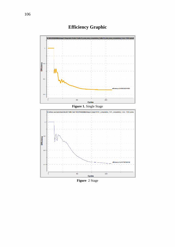
106
Efficiency Graphic
Figure 1. Single Stage
Figure 2 Stage
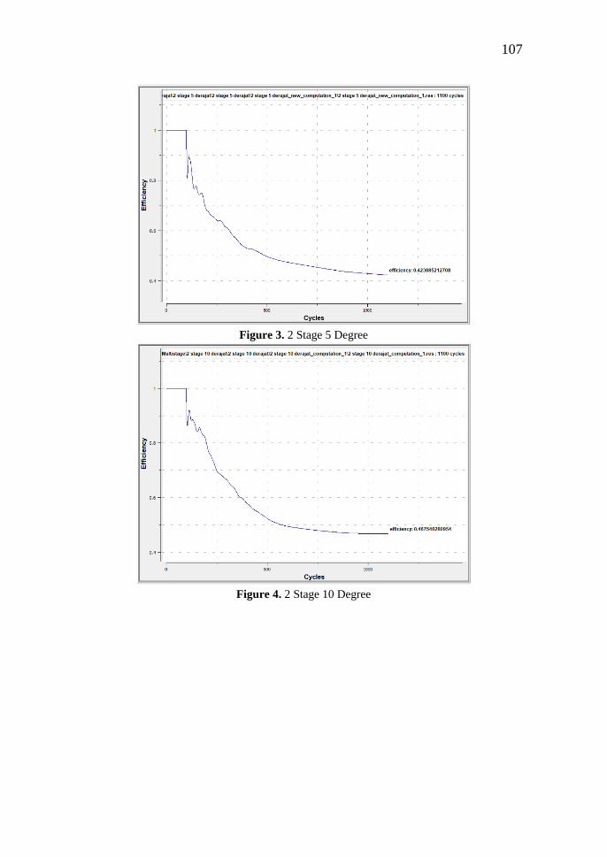
107
Figure 3. 2 Stage 5 Degree
Figure 4. 2 Stage 10 Degree
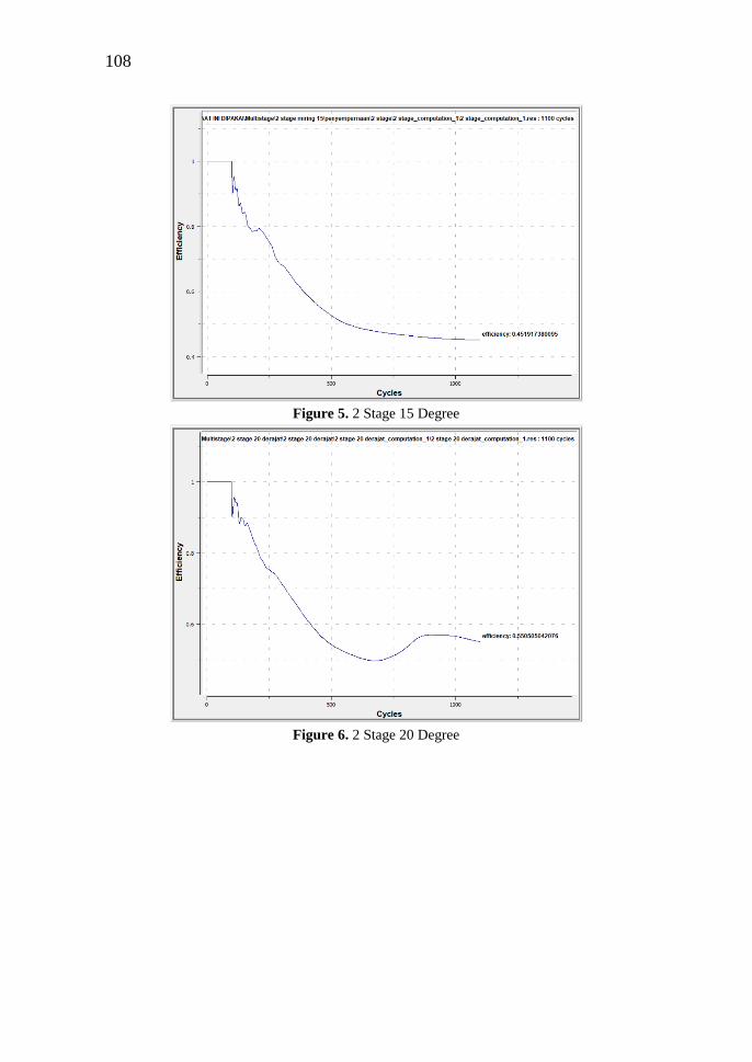
108
Figure 5. 2 Stage 15 Degree
Figure 6. 2 Stage 20 Degree
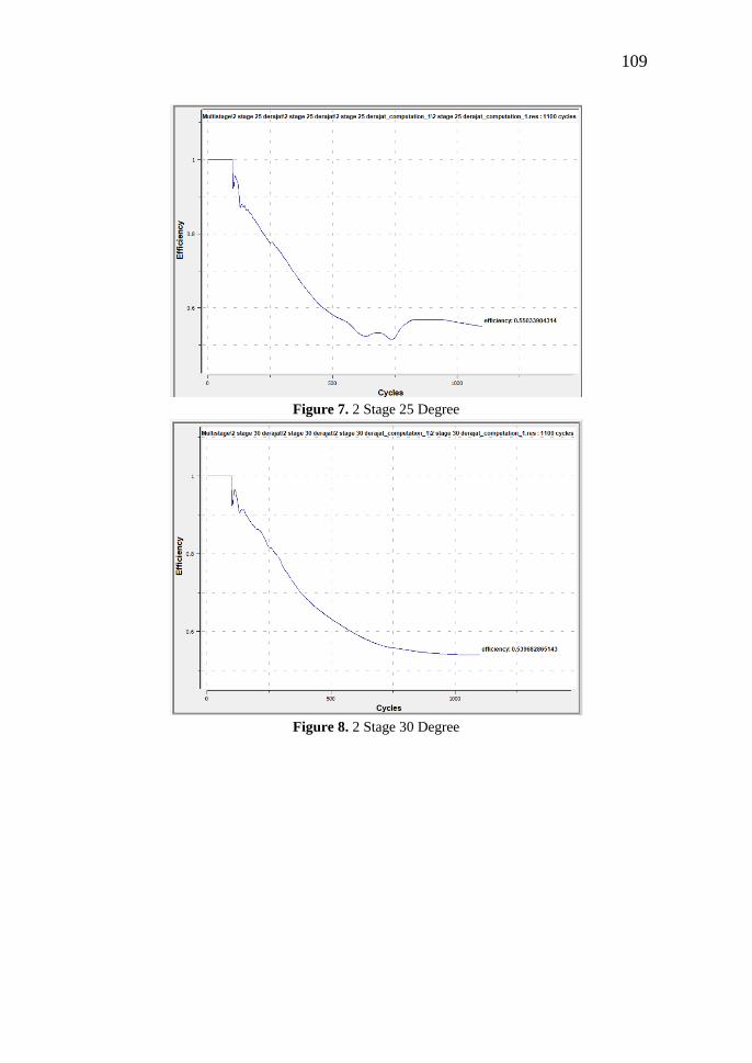
109
Figure 7. 2 Stage 25 Degree
Figure 8. 2 Stage 30 Degree

110
Figure 9. 2 Stage 35 Degree
Figure 10. 2 Stage 40 Degree

111
Figure 11. 2 Stage 45 Degree
Figure 12. 2 Stage 50 Degree
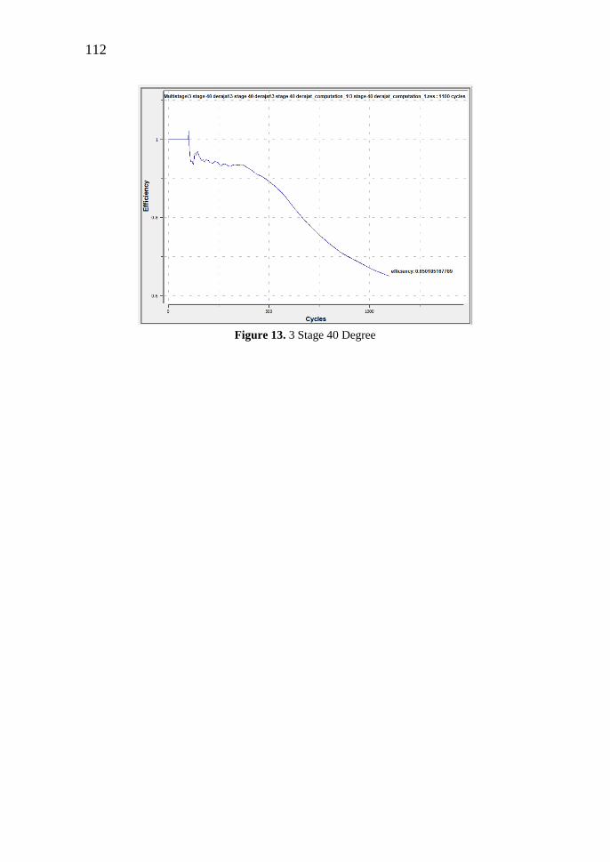
112
Figure 13. 3 Stage 40 Degree

113
Torque Graphic
Figure 1. Single Stage
Figure 2 Stage
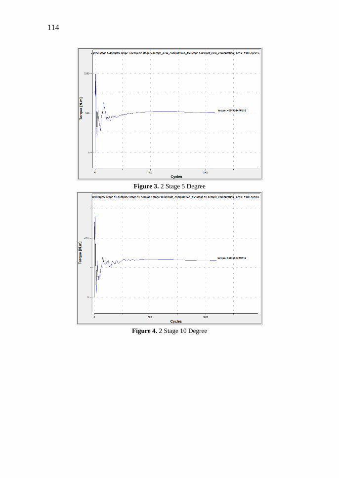
114
Figure 3. 2 Stage 5 Degree
Figure 4. 2 Stage 10 Degree
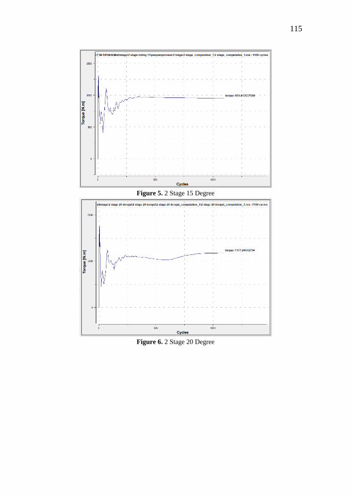
115
Figure 5. 2 Stage 15 Degree
Figure 6. 2 Stage 20 Degree
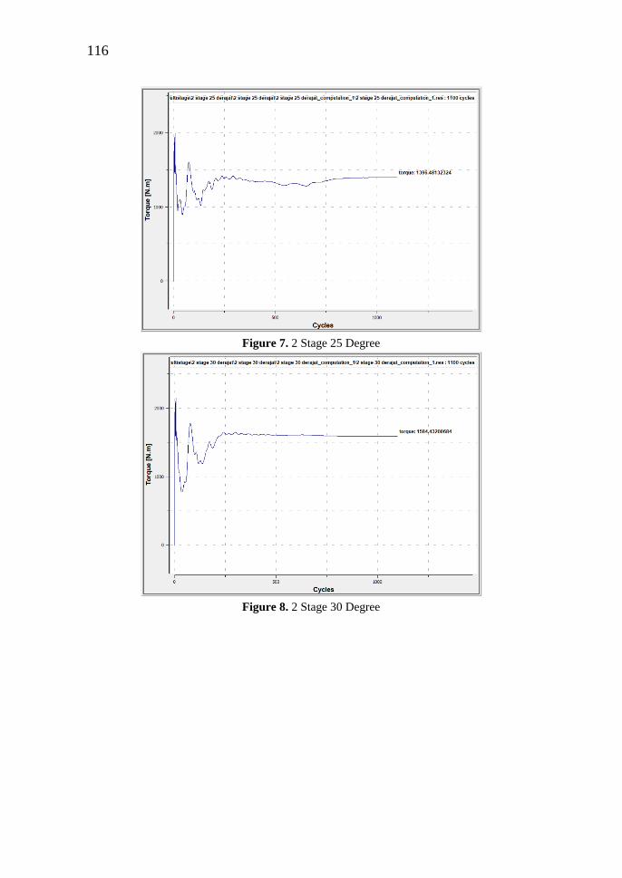
116
Figure 7. 2 Stage 25 Degree
Figure 8. 2 Stage 30 Degree

117
Figure 9. 2 Stage 35 Degree
Figure 10. 2 Stage 40 Degree

118
Figure 11. 2 Stage 45 Degree
Figure 12. 2 Stage 50 Degree

119
Figure 13. 3 Stage 40 Degree

BIOGRAPHY
The author’s name is Desta Rifky Aldara, handsome boy
that was born on December 24th, 1995 in Kudus, Central
Java. Born to be the first son derived from a couple with
father named Zaenal Mutaqin, and mother named
Suwanti. The author had completed the formal studies at
SDN 1 Barongan (2002-2008) for elementary school,
SMPN 2 Kudus (2008-2011) for junior high school, and
SMAN 1 Kudus (2011-2014) for senior high school.
Author proceed to pursue bachelor degree at Department
of Marine Engineering (Double Degree Program with Hochschule Wismar),
Faculty of Marine Technology Institut Teknologi Sepuluh Nopember
Surabaya specializes in marine manufacturing and design. During the study
period, the author active in several campus activities such as: entrepreneurship
staff on HIMASISKAL, staff of PSDM on BEM FTK, Trainer for new student
at Marine Manufacturing and Design Laboratory. For further discussion and
suggestion regarding to this research, the author can be reached through email
stated as below.
Desta Rifky Aldara
+6285774244888
Motto: Make everything simple