Construction and Building Materials 23 (2009) 1487–1494

Contents lists available at ScienceDirect

Construction and Building Materials

journal homepage: www.elsevier .com/locate /conbui ldmat

Design by testing: A procedure for the statistical determination of capacity models

Giorgio Monti a,*, Silvia Alessandri a, Silvia Santini b

a Department of Structural Engineering and Geotechnics, Sapienza University of Rome, Via Antonio Gramsci, 53 – 00197 Rome, Italyb Department of Structures, University of Roma Tre, Via Corrado Segre, 2/6 – 00146 Rome, Italy

a r t i c l e i n f o a b s t r a c t

Article history:Available online 18 September 2008

Keywords:Design assisted by testingCapacity modelsCalibrationFRP debonding strengthExperimental tests

0950-0618/$ - see front matter � 2008 Elsevier Ltd. Adoi:10.1016/j.conbuildmat.2008.07.016

* Corresponding author. Tel.: +39 06 49919197; faxE-mail address: giorgio.monti@uniroma1.it (G. Mo

Worldwide research has now reached a level of integration where an effort towards the harmonization ofprocedures is absolutely needed. Such harmonization may regard, for example, the various steps that leadto the definition of capacity models to be included in design codes, specifically: definition of the testsetup, quantities to be measured, identification of the basic variables influencing the phenomenon, dis-tinction between average values and other fractiles, disaggregation of the model in different partsaccounting for mechanics, fine-tuning and randomnesses, and, finally, assessment of the model againstthe experimental results. Test results and ensuing model developed according to this procedure wouldnaturally lend themselves to be easily shared among the scientific community and would facilitate thetask of calibrating the partial coefficients, with the ambitious aim of attaining a uniform reliability levelamong all capacity equations.

� 2008 Elsevier Ltd. All rights reserved.

1. Introduction

This paper represents a first attempt towards the harmonisationof procedures for the development of capacity design equations tobe included in codes, with the ambitious aim of attaining a uniformreliability level among all of them. The proposed procedure, thoughstill at a preliminary stage of development, will eventually allowresearchers to easily exchange and compare experimental dataand results, to consistently compare accuracy and robustness oftheir respective equations, and to better identify possible sourcesof error in their formulations. It will also allow an easier calibrationof partial coefficients in design codes.

Among the preliminary considerations to facilitate this task, it isnecessary to underline some fundamental issues related to thedevelopment of capacity models.

In our view, the development of capacity models should alwaysbe carried out by looking at the physics of the phenomenon and bytrying to describe the mechanical aspects through an analyticalformulation. In this view, all models should be developed a priori,that is, before any experiment is carried out. Or, at least, the initialpurpose of the experiments is that of giving indications to – and ofconfirming certain intuitions of – the modeller about the observedphenomena; once the model is developed with a clear analyticaldescription of the underlying mechanisms, then (and only then)should numerical comparison with the experimental results becarried out to assess both meaningfulness and accuracy.

ll rights reserved.

: +39 06 49919192.nti).

Unfortunately, too often are regression-based models proposedin the literature. These models are clearly based on a totally differ-ent philosophy, in the sense that they are developed a posteriori,that is, after experiments are performed. The usual procedure isthat of running a large number of tests where all sorts of inputand output variables are measured. Then, a functional form is at-tempted with some coefficient that are calibrated through regres-sion, trying to minimizing the difference with the experimentsoutput. It is now customary to have such models with coefficientsgiven to the highest possible accuracy (up to seven decimal dig-its!), as if the modeller’s ability was only of a numerical nature,rather than related to his/her capability of interpreting, under-standing and representing the mechanical phenomenon. This givesrise to the self-consolatory illusion, among those who follow thisprocess, that they do understand a phenomenon by simply mea-suring ‘how much’ without really having to worry about ‘why’.

As a further fallout of this trend, it should also be underlinedthat professionals, who generally have a practical understandingof resisting mechanisms, hardly find a ‘physical meaning behind’regression-based equations (there actually isn’t). This fosters thetendency to use those equations with no critical sense, especiallyamong younger professionals.

In addition to what commented so far, there are other issuesworth considering.

Ideally, a predictive model should capture the mean behaviour of aphenomenon, that is, it should predict its capacity in an average sense.It would be desirable that all capacity models be given so that theirpredictive line lies at the centre of the experiments’ ‘cloud of points’.In addition to that, the authors should always give the relative errorthat the model yields, for example, in terms of dispersion around

1488 G. Monti et al. / Construction and Building Materials 23 (2009) 1487–1494

the mean. Unfortunately, it is quite customary to develop modelswhose predictive line lies below the experimental cloud, with the jus-tification that, by doing so, the model is ‘safer’, because ‘a large part ofthe experimental points lies above and this provides the model withan inherent safety’. This way of reasoning brings a certain confusion inthose who are using the formulation, because modelling concepts aremixed up with reliability concepts, whereas these two aspects shouldbe treated at different and subsequent stages.

A similar typical mistake that is usually made is the following: amodel is developed and a functional form is found where thecapacity is shown to depend on some basic variables. Then, com-parison to experimental results is usually carried out by introduc-ing the mean values of the basic variables into the formula. Afterhaving checked that the formula correctly predicts the phenome-non on the average, the next (wrong) step is that of replacing inthe formula the mean values of the basic variables with eithercharacteristic or design values, thus thinking that the outcome ofthe formula automatically will predict either the characteristic Xk

or the design value Xd of the capacity. While this is true for linearformulas, it certainly does not apply to non linear equations. Thatis to say that, if a predictive functional form of a capacity rt hasbeen developed as rt ¼ gtðXÞ, where X is the basic variables vector,in general we have that: rtk–gtðXkÞ and rtd–gtðXdÞ.

Thus, it would be desirable that a capacity equation be devel-oped with the following features:

– It should predict the phenomenon on the average (i.e., it shouldpass through the centre of the experimental ‘cloud of points’). Nosafety-related issues should be introduced at this stage.

– The dispersion of the theoretical predictions with respect to theexperiments should always be given (the relative error of themodel), e.g., in terms of coefficient of variation. This will servefor a subsequent calibration of the equation’s reliability. – The transformation of the predictive model into a design modelshould be carried out in a rigorous way, with due consideration ofthe probability distribution of the capacity model, in order to cor-rectly attain the desired fractile.

By following these steps, the scientific community could benefitfrom a common procedure to produce capacity equations to beeasily and consistently compared. In particular, the main advan-tage could be that all design equations will finally attain a uniformreliability level.

The proposed process also has the noticeable advantage of sep-arating the various responsibilities and roles in the development ofa design equation: in the first instance, there is the theoreticaldevelopment, which should only look at the physics/mechanicsof the problem and provide an accurate analytical interpretation;then, the experimental part is carried out to prove that the inter-pretation given predicts the real phenomenon with a certain accu-racy; then, there is a step of clear statistical nature, where theprobability aspects of the formulation (dispersion, errors, fractiles,etc.) are evaluated and, possibly, a further fine-tuning of the equa-tions may be performed; finally, there is the step where the formu-lation is endowed with reliability-based features, with thedefinition of the appropriate partial coefficients.

In the following, all the above concepts, with the only exceptionof the last step, are described in detail and subsequently applied toa capacity equation as an applicative example.

2. Assumptions

In the following sections the steps to be undertaken for a properand consistent development of a capacity model, in the sense trea-

ted above, are presented in detail. Inspiration for the procedurecame from [1]. The following assumptions are made:

(1) A ‘‘sufficient” number of test results is available (this pointwill be better clarified in the next section).

(2) All main geometrical and mechanical quantities are mea-sured in the experimental tests carried out to validate the analyt-ical model.

(3) All random variables are normally distributed.

3. Description of the procedure

Step 1. Development of a theoretical strength modelGiven a capacity mechanism, an analytical model can be devel-

oped based on the a priori understanding of the underlying physicsof the problem (as opposed to a posteriori regression-based models,which are instead based on the outcomes of purposely carried outexperimental tests). The model can be given as

rt ¼ b� gtðXÞ ð1Þ

where gtðXÞ is the capacity model, as function of all basic variables Xthought to be affecting the phenomenon to be modelled, and b is aleast-squares fine-tuning parameter accounting for all other vari-ables (or, secondary phenomena) not included in the theoreticalmechanical model (e.g., either because they are deemed irrelevant,or because their effect is not perfectly understood, or because theydo not fit into the formulation, or because the model is intentionallykept simple).

Step 2. Measurement of the basic variables in testsAfter having defined a theoretical model, and only at this stage,

should it be validated against some experimental results. In thetests, all (geometrical and mechanical) basic variables should bemeasured for each specimen and should be available for the mod-el’s validation.

Geometrical quantities are usually easily measured. For as re-gards mechanical quantities (e.g., material properties), measuresshould be taken according to one of the following methods:

(1) Extracting a sample from each specimen before testing.(2) Cutting one or more portions of each specimen.(3) Non-destructive testing, after calibration on other similar

specimens.

If it is not possible to measure all basic variables of each speci-men, destructive tests shall be carried out on purposely preparedsets of material specimens (e.g., concrete cubes). Here, mean valuesof the variables are obtained, as opposed to the previous threeitems, where point values of the variables are obtained.

In order to be considered as ‘‘sufficient”, the number of tests tocarry out should be as follows:

(1) If point values of the basic variables are available for eachtested specimen, a single test should be carried out for each basicvariables set Xi; when validating the model results rt against theexperimental results re (see Step 3), comparisons should be madein terms of point values (i.e., test by test, as explained at the nextstep).

(2) If mean values of the basic variables are available for eachgroup of tested specimens, a minimum number of 5 tests (a testset) should be carried out for each basic variables set Xi, withi = 1. . .5, in order to get a reasonable estimate Xkm of the mean val-ues of the basic variables set in the kth test set; when validatingthe model results rt against the experimental results re (see Step3), comparisons should be made in terms of mean values (i.e., testset by test set, as explained at the next step).

G. Monti et al. / Construction and Building Materials 23 (2009) 1487–1494 1489

Step 3. Model-experimental results comparison and fine-tuningHere, the parameter b is used to fine-tune the prediction capa-

bility of the theoretical model. One should proceed as follows:

(1) The (mean or point) values of the measured properties areplaced in the capacity function gtðXÞ to obtain the (mean or point)theoretical capacity value rt to be compared with the (mean orpoint) experimental value re.

(2) The correction coefficient b is computed by the least-squaremethod to minimize the difference between theoretical rt andexperimental re values:

minX

i

ðrti � reiÞ2" #

or minX

k

ðrtkm � rekmÞ2" #

ð2Þ

where: rti is the theoretical capacity computed by plugging thepoint values Xi of the basic variables used in test i into the functiongtðXÞ and rei is the experimental capacity obtained from the i-thtest; rtkm is the theoretical capacity computed by plugging the meanvalues Xkm of the basic variables used in test set k into the functiongtðXÞ and rekm is the experimental capacity obtained as the meanfrom the kth test set.

At this stage, the correspondence of the test results with the ini-tial model hypotheses should be checked. Particularly, in order toverify the model significance, if the difference between theoreticalrt and experimental re values is unacceptably large (say, more than40% in terms of normalised values), one should try and reduce it byeither:

(1) reformulating the theoretical model with a better interpre-tation of the underlying physical phenomena, or

(2) enhancing the theoretical model to include previouslyneglected variables, or

(3) increasing the number of (sets of) experiments in order tofine-tune the correction coefficient b.

Step 4. Definition of a probabilistic capacity modelA probabilistic capacity model r should be now defined to in-

clude the inevitable model error (that is, the error remaining evenafter the least-square fine-tuning):

r ¼ rt � d ¼ b� gtðXÞ � d ð3Þ

where d is the model error, represented by a random variable withNormal distribution with mean value dm = 1 and standard deviationrd .

For the estimation of the latter, two different cases might occur:

(1) The values Xi of the basic variables X are available as pointvalues for each test i:

a. The error is evaluated for each test as

di ¼rei

rti¼ rei

b� gtðXiÞð4Þ

where rei and rti are the point values of the experimental capacityand of the theoretical capacity, respectively, for the i-th test.

b. The standard deviation of the error is estimated throughthe sample standard deviation (here, it is considered thatdm = 1):

r̂d ¼

ffiffiffiffiffiffiffiffiffiffiffiffiffiffiffiffiffiffiffiffiffiffiffiffiffiffiffiPni¼1ðdi � 1Þ

n� 1

s; n ¼ number of tests ð5Þ

(2) The values Xkm of the basic variables X are available as meanvalues for each set of k tests:

a. The error is evaluated for each tests set as

dk ¼rekm

rtkm

¼ rekm

b� gtðXkmÞð6Þ

where rekmand rtkm

are the mean values of the experimental capacityand of the theoretical capacity, respectively, for the kth test set.

b. The standard deviation of the error is estimated through thesample standard deviation (here, it is considered thatdm = 1):

r̂d ¼

ffiffiffiffiffiffiffiffiffiffiffiffiffiffiffiffiffiffiffiffiffiffiffiffiffiffiffiffiPmk¼1ðdk � 1Þ

m� 1

s; m ¼ number of test sets ð7Þ

For what concerns the basic variables variation, if the test pop-ulation is fully representative of the population, the coefficients ofvariation VXi

of the basic variables can be directly determined fromthe test data. In most cases, the coefficients of variation are deter-mined based on a priori knowledge.

Step 5. Estimation of mean and variance of the capacity modelThe characteristic value of the capacity model should be sought

starting from its statistics, under the normality assumption. For theabove-defined probabilistic function r = r � d = b � gt(X) � d, thefirst-order approximation of the mean is (since dm = 1):

rm ¼ EðrÞ� b� gtðXmÞ ð8Þ

The first-order approximation of the variance is

VarðrÞ ¼X

i

c2i � VarðXiÞ

� �þ c2

d � VarðdÞ

þX

i

Xn

j–i

ci � cj � CovðXiXjÞ� �

ð9Þ

where ci ¼ oroXi

���Xm ;dm

and cd ¼ orod

��Xm ;dm

are the values of the partial

derivatives of the function r with respect to the basic variables Xi

and to the error d, respectively, computed at the mean values ofXi and d, and where the covariance Cov(Xi Xj) is given by

CovðXiXjÞ ¼ E½ðXi � XimÞðXj � XjmÞ� ¼ EðXiXjÞ � EðXiÞEðXjÞ

¼ 1n

Xn

l¼1

ðXil � XimlÞðXjl � XjmlÞ ð10Þ

If the basic variables are considered as statistically independent,the last term in Eq. (9) is zero.

Step 6. Estimation of the characteristic value of the capacity modelHaving computed the statistics of the capacity model, the

expression correctly representing its characteristic value rk is final-ly found as

rk ¼ rm � 1:64� ½VarðrÞ�1=2 ð11Þ

Step 7. Check of the error propertiesTo check if the residuals (model errors) satisfy the initial

hypothesis, some tests must be performed:

(1) Check of the normality hypothesis of error (normality ofresiduals): an assumed probability distribution can be verified by:

a. Construction of the probability graph:The assumed distribution model can be checked by visually com-paring the frequency diagram with the density function.To thisaim, the observations x1, x2,...,xn must be arranged in increasingorder and each value must be plotted at the cumulative probabilitym/(n + 1), where m is the number of the single observation in theobservation order and n is the total number of observations [2].If the resulting graph of data points shows a linear or approxi-mately linear trend that fits the straight line passing through the

1490 G. Monti et al. / Construction and Building Materials 23 (2009) 1487–1494

points (0.5, xm) and (0.84, x.84), where xm is the mean value of thevariate X and x.84 is the value with probability p = 0.84, the normaldistribution is applicable to the model error.

b. Execution of a ‘‘goodness-of-fit” test as the Kolmogorov–Smirnov test (K-S) or the chi-square (v2) test.

(2) Check of the hypothesis of omoschedasticity of error:Thetest for the omoschedasticity of the error allows to verify if the var-iance of the residuals does not vary with respect to the indepen-dent variate; the error variability must be plotted vs. the capacityvariability; if the residuals are regularly arranged, the model is wellspecified.

4. Application

For the sake of exemplification, the procedure explained aboveis here applied for developing a consistent formula for the charac-teristic debonding strength of an FRP strengthening. Of course, theprocedure may be applied to any capacity formula.

Step 1. Development of a theoretical strength modelSeveral formulations have been developed for the debonding

strength of FRP fabrics externally bonded to concrete. A possibleone, which is here studied for demonstration purposes, is the onegiven in the Italian CNR Guidelines [3]. There, the debondingstrength is expressed as a certain function of some basic variables(here, only the functional form is retained, with no consideration ofcharacteristic/design values for the basic variables):

ffd ¼

ffiffiffiffiffiffiffiffiffiffiffiffiffiffiffiffiffiffiffiffiffiffiffiffiffiffiffiffiffiffiffiffiffiffiffiffiffiffiffiffiffi2kGkb � Ef

ffiffiffiffiffiffiffiffiffiffiffiffiffiffifc � fct

ptf

sð12Þ

where kG is a least-square fine-tuning parameter (what above wascalled b); kb is a geometric model parameter depending on thewidth of both the strengthened beam and the FRP system; Ef, fc

and fct are, respectively, the Young’s modulus of FRP strengthening,the concrete compression strength, and the concrete tensilestrength, respectively; tf is the FRP strengthening thickness. Hereonly the mechanical parameters (Ef, fc, fct) have been assumed as ba-sic variables; the geometrical parameters kb, tf are considered asdeterministic, owing to their negligible variance.

Step 2. Measurement of the basic variables in testsThe procedure is here applied using experimental test results

from the literature (Table 1) [4–8]; it should be noted that in allcollected cases the basic variables Ef, fc and fct are given in termsof mean values obtained from tests on samples extracted fromthe specimens before testing.

Step 3. Model-experimental results comparison and fine-tuningThe model is fine-tuned by calibration of the coefficient kG,

which should be carried out by comparing the theoretical valuesof the debonding strength with the experimental ones. Throughthe least-squares method, the value of kG is determined so to min-imize the difference between the experimental value of the maxi-mum debonding force, Fmax,e, and the theoretical one, given by:

Fmax;t ¼ bf � tf � ffd ¼ bf

ffiffiffiffiffiffiffiffiffiffiffiffiffiffiffiffiffiffiffiffiffiffiffiffiffiffiffiffiffiffiffiffiffiffiffiffiffiffiffiffiffiffiffiffiffiffiffiffiffiffi2kGkb � tf � Ef

ffiffiffiffiffiffiffiffiffiffiffiffiffiffifc � fct

pqð13Þ

where bf is the width of the FRP.Because in the available test results in Table 1 the basic vari-

ables Ef, fc and fct are given as mean values, fine-tuning of the coef-ficient kG has been carried out by comparing, for each test set, theexperimental mean values Fmax;em to the mean theoretical valuesFmax;tm , given by

Fmax;tm ¼ bf � tf � ffdm ¼ bf

ffiffiffiffiffiffiffiffiffiffiffiffiffiffiffiffiffiffiffiffiffiffiffiffiffiffiffiffiffiffiffiffiffiffiffiffiffiffiffiffiffiffiffiffiffiffiffiffiffiffiffiffiffiffiffiffiffiffiffi2kGkb � tf � Efm

ffiffiffiffiffiffiffiffiffiffiffiffiffiffiffiffiffiffiffiffifcm � fctm

pqð14Þ

The value of the so-obtained least-square fine-tuning parameter iskG = 0.107. A comparison between theoretical and experimental re-sults is given in Fig. 1. The available experimental tests are groupedaccording both geometrical and mechanical properties.

Step 4. Definition of the probabilistic capacity modelThe assumed probabilistic model of the capacity is

ffd ¼

ffiffiffiffiffiffiffiffiffiffiffiffiffiffiffiffiffiffiffiffiffiffiffiffiffiffiffiffiffiffiffiffiffiffiffiffiffiffiffiffiffi2kGkb � Ef

ffiffiffiffiffiffiffiffiffiffiffiffiffiffifc � fct

ptf

s� d ð15Þ

where d is a random variable with unit mean and standard devia-tion rd.The error d in the equation of ffd is evaluated as the ratio be-tween theoretical and experimental values of the maximum forceFmax; using the tests results in Table 1, it is possible to calculatethe mean value, assumed as unit value, and the variance, given by:

VarðdÞ ¼ VarFmax;e

Fmax;t

� �¼ 0:12 ð16Þ

The basic random variables Ef, fc and fct are considered as statis-tically independent among them. As for the coefficients of varia-tion, for fc and fct a value of Vfc ¼ Vfct ¼ 0:2 has been assumed,while for Ef a value of VEf

¼ 0:0 has been taken.Step 5. Estimation of mean and variance of the capacity modelAccording to Eq. (8), the mean value of the debonding strength

is

ffdm ¼

ffiffiffiffiffiffiffiffiffiffiffiffiffiffiffiffiffiffiffiffiffiffiffiffiffiffiffiffiffiffiffiffiffiffiffiffiffiffiffiffiffiffiffiffiffiffiffiffiffiffi2kGkb � Efm

ffiffiffiffiffiffiffiffiffiffiffiffiffiffiffiffiffiffiffiffifcm � fctm

ptf

sð17Þ

The variance of a random variable y =Q

ix � d is given by:

VarðyÞ ¼X

i

c2i � VarðxiÞ

� �þ c2

d � VarðdÞ ð18Þ

where the coefficients ci are the values of the partial derivatives ofthe function y with respect to the basic variables xi, calculated at themean values of the basic variables and cd is the values of the partialderivatives of the function y with respect to the error variable d. Thepartial derivatives of the ffd function, with respect to the basic vari-ables are

offd

oEf

� ¼ 1

2k1 � E�1=2

fm � ðfcm � fctmÞ1=4 ð19Þ

offd

ofc

� ¼ 1

4k1 � E1=2

fm � f�3=4cm � f 1=4

ctm ð20Þ

offd

ofct

� ¼ 1

4k1 � E1=2

fm � f 1=4cm � f�3=4

ctm ð21Þ

offd

od

� ¼ k1 � E1=2

fm � f 1=4cm � f 1=4

ctm ð22Þ

where

k1 ¼

ffiffiffiffiffiffiffiffiffiffiffiffiffi2kGkb

tf

sð23Þ

Therefore the variance of ffd is given by

VarðffdÞ ¼12

k1 � E�1=2fm � ðfcm � fctmÞ1=4

� �2

� VarðEfÞ

þ 14

k1 � E1=2fm � f�3=4

cm � f 1=4ctm

� �2

� VarðfcÞ

þ 14

k1 � E1=2fm � f 1=4

cm � f�3=4ctm

� �2

� VarðfctÞ

þ k1 � E1=2fm � f 1=4

cm � f 1=4ctm

h i2� VarðdÞ ð24Þ

Which can be simplified as

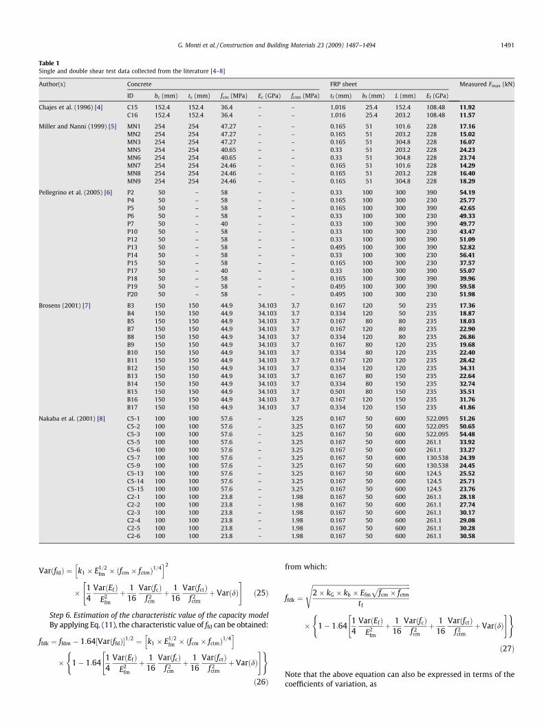
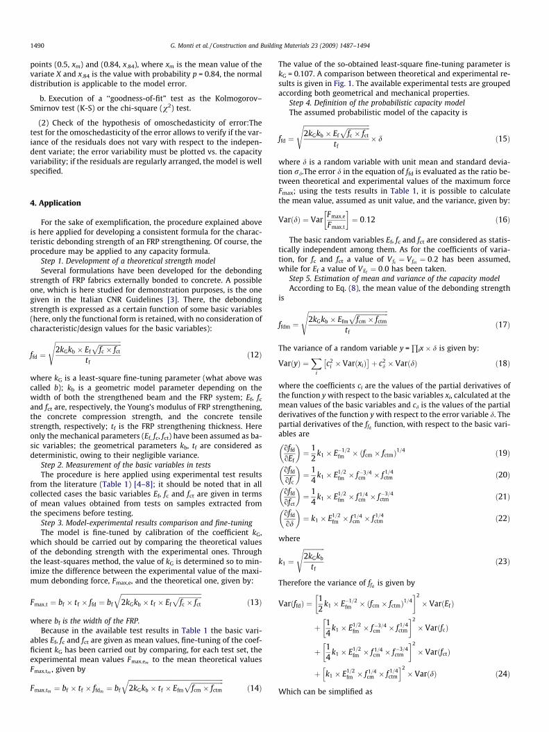
Table 1Single and double shear test data collected from the literature [4–8]

Author(s) Concrete FRP sheet Measured Fmax (kN)

ID bc (mm) tc (mm) fcm (MPa) Ec (GPa) fctm (MPa) tf (mm) bf (mm) L (mm) Ef (GPa)

Chajes et al. (1996) [4] C15 152.4 152.4 36.4 – – 1.016 25.4 152.4 108.48 11.92C16 152.4 152.4 36.4 – – 1.016 25.4 203.2 108.48 11.57

Miller and Nanni (1999) [5] MN1 254 254 47.27 – – 0.165 51 101.6 228 17.16MN2 254 254 47.27 – – 0.165 51 203.2 228 15.02MN3 254 254 47.27 – – 0.165 51 304.8 228 16.07MN5 254 254 40.65 – – 0.33 51 203.2 228 24.23MN6 254 254 40.65 – – 0.33 51 304.8 228 23.74MN7 254 254 24.46 – – 0.165 51 101.6 228 14.29MN8 254 254 24.46 – – 0.165 51 203.2 228 16.40MN9 254 254 24.46 – – 0.165 51 304.8 228 18.29

Pellegrino et al. (2005) [6] P2 50 – 58 – – 0.33 100 300 390 54.19P4 50 – 58 – – 0.165 100 300 230 25.77P5 50 – 58 – – 0.165 100 300 390 42.65P6 50 – 58 – – 0.33 100 300 230 49.33P7 50 – 40 – – 0.33 100 300 390 49.77P10 50 – 58 – – 0.33 100 300 230 43.47P12 50 – 58 – – 0.33 100 300 390 51.09P13 50 – 58 – – 0.495 100 300 390 52.82P14 50 – 58 – – 0.33 100 300 230 56.41P15 50 – 58 – – 0.165 100 300 230 37.57P17 50 – 40 – – 0.33 100 300 390 55.07P18 50 – 58 – – 0.165 100 300 390 39.96P19 50 – 58 – – 0.495 100 300 390 59.58P20 50 – 58 – – 0.495 100 300 230 51.98

Brosens (2001) [7] B3 150 150 44.9 34.103 3.7 0.167 120 50 235 17.36B4 150 150 44.9 34.103 3.7 0.334 120 50 235 18.87B5 150 150 44.9 34.103 3.7 0.167 80 80 235 18.03B7 150 150 44.9 34.103 3.7 0.167 120 80 235 22.90B8 150 150 44.9 34.103 3.7 0.334 120 80 235 26.86B9 150 150 44.9 34.103 3.7 0.167 80 120 235 19.68B10 150 150 44.9 34.103 3.7 0.334 80 120 235 22.40B11 150 150 44.9 34.103 3.7 0.167 120 120 235 28.42B12 150 150 44.9 34.103 3.7 0.334 120 120 235 34.31B13 150 150 44.9 34.103 3.7 0.167 80 150 235 22.64B14 150 150 44.9 34.103 3.7 0.334 80 150 235 32.74B15 150 150 44.9 34.103 3.7 0.501 80 150 235 35.51B16 150 150 44.9 34.103 3.7 0.167 120 150 235 31.76B17 150 150 44.9 34.103 3.7 0.334 120 150 235 41.86

Nakaba et al. (2001) [8] C5-1 100 100 57.6 – 3.25 0.167 50 600 522.095 51.26C5-2 100 100 57.6 – 3.25 0.167 50 600 522.095 50.65C5-3 100 100 57.6 – 3.25 0.167 50 600 522.095 54.48C5-5 100 100 57.6 – 3.25 0.167 50 600 261.1 33.92C5-6 100 100 57.6 – 3.25 0.167 50 600 261.1 33.27C5-7 100 100 57.6 – 3.25 0.167 50 600 130.538 24.39C5-9 100 100 57.6 – 3.25 0.167 50 600 130.538 24.45C5-13 100 100 57.6 – 3.25 0.167 50 600 124.5 25.52C5-14 100 100 57.6 – 3.25 0.167 50 600 124.5 25.71C5-15 100 100 57.6 – 3.25 0.167 50 600 124.5 23.76C2-1 100 100 23.8 – 1.98 0.167 50 600 261.1 28.18C2-2 100 100 23.8 – 1.98 0.167 50 600 261.1 27.74C2-3 100 100 23.8 – 1.98 0.167 50 600 261.1 30.17C2-4 100 100 23.8 – 1.98 0.167 50 600 261.1 29.08C2-5 100 100 23.8 – 1.98 0.167 50 600 261.1 30.28C2-6 100 100 23.8 – 1.98 0.167 50 600 261.1 30.58

G. Monti et al. / Construction and Building Materials 23 (2009) 1487–1494 1491

VarðffdÞ ¼ k1 � E1=2fm � ðfcm � fctmÞ1=4

h i2

� 14

VarðEfÞE2

fm

þ 116

VarðfcÞf 2cm

þ 116

VarðfctÞf 2ctm

þ VarðdÞ" #

ð25Þ

Step 6. Estimation of the characteristic value of the capacity modelBy applying Eq. (11), the characteristic value of ffd can be obtained:

ffdk ¼ ffdm � 1:64½VarðffdÞ�1=2 ¼ k1 � E1=2fm � ðfcm � fctmÞ1=4

h i

� 1� 1:6414

VarðEf ÞE2

fm

þ 116

VarðfcÞf 2cm

þ 116

VarðfctÞf 2ctm

þ VarðdÞ" #( )

ð26Þ

from which:

ffdk ¼

ffiffiffiffiffiffiffiffiffiffiffiffiffiffiffiffiffiffiffiffiffiffiffiffiffiffiffiffiffiffiffiffiffiffiffiffiffiffiffiffiffiffiffiffiffiffiffiffiffiffiffiffiffiffiffiffiffiffiffiffiffi2� kG � kb � Efm

ffiffiffiffiffiffiffiffiffiffiffiffiffiffiffiffiffiffiffiffifcm � fctm

ptf

s

� 1� 1:6414

VarðEfÞE2

fm

þ 116

VarðfcÞf 2cm

þ 116

VarðfctÞf 2ctm

þ VarðdÞ" #( )

ð27Þ

Note that the above equation can also be expressed in terms of thecoefficients of variation, as

0

10

20

30

40

50

60

70

80

0 10 20 30 40 50 60 70

Fm

ax,t

Fmax ,e

Experimental  tests:

08

Cahajies et al. (1996)

Miller and Nanni (1999)

Pellegrino et al. (2005)

Brosens (2001)

Nakaba et al. (2001)

Fig. 1. Comparison between theoretical and experimental results.

Table 2Model error d

m d (m/n + 1)

1 0.45 0.0452 0.47 0.0913 0.52 0.1364 0.56 0.1825 0.57 0.2276 0.57 0.2737 0.83 0.3188 0.97 0.3649 0.99 0.40910 1.02 0.45511 1.07 0.50012 1.07 0.54513 1.11 0.59114 1.18 0.63615 1.19 0.68216 1.30 0.72717 1.33 0.77318 1.35 0.81819 1.40 0.86420 1.47 0.90921 1.57 0.955

1492 G. Monti et al. / Construction and Building Materials 23 (2009) 1487–1494

ffdk ¼

ffiffiffiffiffiffiffiffiffiffiffiffiffiffiffiffiffiffiffiffiffiffiffiffiffiffiffiffiffiffiffiffiffiffiffiffiffiffiffiffiffiffiffiffiffiffiffiffiffiffiffiffiffiffiffiffiffiffiffiffiffi2� kG � kb � Efm

ffiffiffiffiffiffiffiffiffiffiffiffiffiffiffiffiffiffiffiffifcm � fctm

ptf

s

� 1� 1:6414

V2Efþ 1

16V2

fcþ 1

16V2

fctþ VarðdÞ

� � �ð28Þ

0

0.2

0.4

0.6

0.8

1

1.2

1.4

1.6

1.8

0 10 20 30 40 5

Mod

el e

rror

,δ

Cumulative pro

Fig. 2. Model error plotted

which, with the assumptions made above on the coefficients of var-iation and the value computed in Eq. (16), becomes:

ffdk ¼ 0:4

ffiffiffiffiffiffiffiffiffiffiffiffiffiffiffiffiffiffiffiffiffiffiffiffiffiffiffiffiffiffiffiffiffiffiffiffiffiffiffiffiffiffiffiffiffiffiffiffiffiffiffiffiffiffiffiffiffiffiffiffi2� kG � kb � Efm

ffiffiffiffiffiffiffiffiffiffiffiffiffiffiffiffiffiffiffifcm � f9m

ptf

sð29Þ

Note that: (a) the equation yielding the ‘true’ characteristic value ofthe capacity is now expressed in terms of the mean values of the ba-sic variables, (b) their variability is contained within the externalcoefficient (0.4), which also includes the model error and (c) thecoefficient kG has the meaning of a fine-tuning coefficient.

Step 7. Check of the error properties

(1) Check of the normality hypothesis of error (normality ofresiduals):

a. Construction of the normal probability graph: The data forthe model error d obtained from the tests listed in Table 1, as pre-viously described, are arranged in increasing order and are plottedat the cumulative probability m/(n + 1) (Table 2).The resultinggraph of data points (Fig. 2) shows a linear trend that fit thestraight line passing through the points (0.5, dm = 1) and (0.84,d.84 = 1.346), where dm is the mean value of the model error d,and d.84 = dm + rd = 1.346 is the value with probability p = 0.84;the normal distribution is therefore applicable to the model error.

b. Kolmogorov–Smirnov test for the normality of residuals: Thevalidity of the assumed Normal distribution is validated also by theKolmogorov–Smirnov ‘‘goodness-of-fit test”:

1. For a sample of dimension n where data are in ascendingorder, the cumulative distribution function is defined as

0 60 70 80 90 100

bability = m/(N+1)

Normal (1,0.35)

data

on a probability paper.

Table 3Critical values of Da

n in the Kolmogorov–Smirnov test [2]

Dan 0.2 0.1 0.05 0.01

5 0.45 0.51 0.56 0.6710 0.32 0.37 0.41 0.4915 0.27 0.30 0.34 0.4020 0.23 0.26 0.29 0.3625 0.21 0.24 0.27 0.3230 0.19 0.22 0.24 0.2935 0.18 0.20 0.23 0.2740 0.17 0.19 0.21 0.2545 0.16 0.18 0.20 0.2450 0.15 0.17 0.19 0.23

>50 1:07=ffiffiffinp

1:22=ffiffiffinp

1:36=ffiffiffinp

1:63=ffiffiffinp

G. Monti et al. / Construction and Building Materials 23 (2009) 1487–1494 1493

SnðdÞ ¼0 d < d1hn dh � d < dn

1 d � dn

8><>: ð30Þ

2. The maximum difference is computed between Sn(d) andthe theoretical cumulative distribution function (CDF)F(d) = N(dm,rd)

Dn ¼maxdjFðdÞ � SnðdÞj ¼ 0:177 ð31Þ

0

0.1

0.2

0.3

0.4

0.5

0.6

0.7

0.8

0.9

1

0 0.2 0 .4 0.6 0.8

Cum

ulat

ive

dist

ribut

ion

func

tion,

CD

F

Dn

Mode

Fig. 3. Cumulative distributi

0

0.2

0.4

0.6

0.8

1

1.2

1.4

1.6

1.8

0 10 20 30Fm

Mod

el e

rror

,δ

Fig. 4. Check of the hypothesis of om

3. The observed value Dn is compared to the critical value Dan ,

which is that value by which:

PðDn � DanÞ ¼ 1� a ð32Þ

The test is here performed at the 5% significance level (a = 0.05).The critical value of Da

n ¼ 0:286 is evaluated by numerical interpo-lation from Table 3; since it is verified that the maximum discrep-ancy is less than Da

n ¼ 0:286, the Normal distribution hypothesisis verified at the 5% significance level (see Fig. 3).

(2) Check of the hypothesis of omoschedasticity of error: Toverify the hypothesis of omoschedasticity of error, the residualsare plotted vs. the theoretical maximum force Fmax,t (Fig. 4); thepoints on the graph cover an homogeneous area around the hori-zontal line at dm = 1; this means that the variance of the residualsdoes not vary with respect to the independent variate and thusthe model is well specified.

4.1. Comparison with the capacity model in [3]

In the capacity model of the debonding strength ffd described in[3], the parameter kG is calibrated on the basis of experimental testsin order to obtain the characteristic value of ffd. The statistical anal-ysis of tests results had provided an mean value kGm ¼ 0:064 and astandard deviation rkG ¼ 0:023; the 5th percentile of the statistical

1 1.2 1.4 1.6 1.8

Sn(d)

CDF

Sn( )

l error,δ

on of the model error d.

40 50 60 70 80

ax ,t

Experimental tests:Cahajies et al. (1996)

Miller and Nanni (1999)

Pellegrino et al. (2005)

Brosens (2001)

Nakaba et al. (2001)

oschedasticity of the residuals.

1494 G. Monti et al. / Construction and Building Materials 23 (2009) 1487–1494

distribution had been found as kGk¼ 0:026. The characteristic value

of the debonding strength was then obtained by plugging in theequation the characteristic values of both the concrete compressionstrength, fck, and the parameter kG (therein rounded to 0.03), whilethe other variables were given as mean values:

ffdk ;CNR ¼

ffiffiffiffiffiffiffiffiffiffiffiffiffiffiffiffiffiffiffiffiffiffiffiffiffiffiffiffiffiffiffiffiffiffiffiffiffiffiffiffiffiffi2Ef kGkkb

ffiffiffiffiffiffiffiffiffiffiffiffiffiffiffiffiffiffiffifck � fctm

ptf

sð33Þ

The comparison between this formula and that (29) obtained withthe proposed procedure shows that:

ffdk

ffdk;CNR

¼ 0:84 ð34Þ

that is, the equation obtained with proposed rigorous procedureyields capacity values that are approximately 15% lower than thoseobtained with the formula appearing in [3], thus showing that thereare cases where the approximations introduced as highlighted inthe introduction to this paper in some formulations, often lead tonon-conservative estimates of the design values.

5. Conclusions

It has been proposed a procedure to develop, in a consistentmanner, design equations that allow to compute the capacity ofresisting mechanisms with controlled reliability. Also, the proce-dure shows how experimental tests should be treated for fine-tun-ing the model and for arriving at the ‘true’ characteristic value ofthe analytical capacity models.

The paper deals, in methodological terms, with how theoreticalmodels should be developed, with how experimental tests shouldbe performed, especially regarding the parameters to measure,and with how to include the values of the basic variables in theequation of the theoretical model.

Ideally, any capacity model should be developed on the basis oftheoretical considerations and subsequently fine-tuned through aregression analysis based on tests results. The validity of the modelshould then be checked by means of a statistical interpretation ofall available test data. The formulation here proposed then includesin the theoretical model a new variable that represents the model

error. This variable is assumed to be normally distributed whit unitmean and standard deviation to be evaluated from comparisonwith experimental results.

Once the statistical parameters of the model error are known, itis possible to define the statistical parameters of the capacity mod-el and to evaluate its characteristic value, which is the aim forapplication in design.

The proposed procedure is applied to the development of acapacity formula for the debonding strength of FRP, starting froma formulation proposed in the Italian CNR Guidelines. The compar-ison with the latter for the evaluation of the characteristic value ofthe debonding strength shows that a non-rigorous procedure canyield non-conservative values of the capacity.

The proposed procedure is currently being applied to a largeseries of capacity equations, in order to check for their consistencyand reliability.

Acknowledgement

This work has been carried out under the program ‘‘Dipartimen-to di Protezione Civile – Consorzio RELUIS”, signed on 2005-07-11(no. 540), Research Line 2 and 8, whose financial support wasgreatly appreciated.

References

[1] EN-1990, EC0 (Eurocode 0) – Basis of structural design; 1990.[2] Ang AHS, Tang WH. Probability concepts in engineering planning and decision.

Basic principles, vol. 1. New York: John Wiley and Sons; 1975.[3] CNR DT-200/2004. Guide for the Design and Construction of Externally Bonded

FRP Systems for Strengthening Existing Structures, CNR Rome; 2004. <http://www.cnr.it>.

[4] Chajes MJ, Finch Jr WW, Januska TF, Thomson Jr TA. Bond and force transfer ofcomposite material plates bonded to concrete. ACI Struct J 1996;93:208–17.

[5] Miller B, Nanni A. Bond between CFRP sheets and concrete. In: Cincinnati OH,Bank LC, editors. Proceedings of ASCE 5th materials congress; 1999. p. 240–7.

[6] Pellegrino C, Boschetto G, Tinazzi D, Modena C. Progress on understanding bondbehaviour in RC elements strengthened with FRP. In: Proceedings of theinternational symposium on bond behaviour of FRP in structures; 2005.

[7] Brosens K. Anchorage of externally bonded steel plates and CFRP laminates forstrengthening concrete element. Doctoral thesis, Katholieke Universiteit,Leuven; 2001.

[8] Nakaba K, Kanakubo T, Furuta T, Yoshizawa H. Bond behavior between fiber-reinforced polymer laminates and concrete. ACI Struct J 2001;98(3).