Design of a Lithium-ion Battery Pack for PHEV Using a HybridOptimization Method

Nansi Xue1,∗, Wenbo Du1, Thomas A. Greszler3, Wei Shyy2, Joaquim R. R. A. Martins1

Ann Arbor, Michigan, USA

Abstract

This paper outlines a method for optimizing the design of a lithium-ion battery pack for hy-brid vehicle applications using a hybrid numerical optimization method that combines multipleindividual optimizers. A gradient-free optimizer (ALPSO) is coupled with a gradient-based op-timizer (SNOPT) to solve a mixed-integer nonlinear battery pack design problem. This methodenables maximizing the properties of a battery pack subjected to multiple safety and perfor-mance constraints. The optimization framework is applied to minimize the mass, volume andmaterial costs. The optimized pack design satisfies the energy and power constraints exactlyand shows 13.9 – 18% improvement in battery pack properties over initial designs. The optimalpack designs also performed better in driving cycle tests, resulting in 23.1 – 32.8% increase indistance covered per unit of battery performance metric, where the metric is either mass, volumeor material cost.

Keywords: Lithium-ion, Optimization, Hybrid vehicle, Battery pack design

Contents

1 Introduction 1

2 Methodology 32.1 Optimization technique . . . . . . . . . . . . . . . . . . . . . . . . . . . . . . . 32.2 Cell model . . . . . . . . . . . . . . . . . . . . . . . . . . . . . . . . . . . . . . 52.3 Battery model . . . . . . . . . . . . . . . . . . . . . . . . . . . . . . . . . . . . 6

3 Problem formulation 6

4 Results and discussion 84.1 Discharge profile . . . . . . . . . . . . . . . . . . . . . . . . . . . . . . . . . . 84.2 Optimization results . . . . . . . . . . . . . . . . . . . . . . . . . . . . . . . . . 94.3 Driving cycle test . . . . . . . . . . . . . . . . . . . . . . . . . . . . . . . . . . 14

∗Corresponding author: courtrun@umich.edu1Department of Aerospace Engineering, University of Michigan2Department of Mechanical Engineering, Hong Kong University of Science and Technology3Saft America Inc., Cockeysville, MD

Preprint submitted to Applied Energy October 30, 2013

5 Conclusions 17

1. Introduction

Hybrid vehicles are becoming increasingly common as automakers make use of alternativeenergy storage systems to improve vehicle performance and efficiency [1, 2], and to reduce theirenvironmental impact [3]. Among the alternative energy storage systems, lithium-ion batteriesare a popular choice due to their high energy densities and cycling durability [4]. Plug-in hybridelectric vehicles (PHEV) incorporate these batteries to provide all-electric driving range for dailycommuting. The main problem with lithium-ion batteries is that their energy density is orders ofmagnitude lower than that of gasoline. As such, the lithium-ion battery packs on PHEVs tend tobe heavy, bulky and expensive. This limits the all-electric driving range the PHEV can sustain,and hence reduces the advantages of the hybrid drivetrain. Therefore, an optimally designedbattery system is essential to maximize the potential benefits of PHEV.

Lithium-ion electrochemical modeling has been well studied in the past 20 years, with modelsof varying degrees of fidelity being introduced. Doyle and Newman [5] introduced a continuumformulation to model the ion transport and kinetics within an electrochemical cell. Equivalentcircuit models simplify cell mechanisms and reduce a battery to a few parameters identified bysimplified circuits [6, 7]. These models have been subsequently applied to analyze battery per-formance in electric vehicle operations [8, 9]. Ramadesigan et al. [10] provided a comprehensiveoverview of various model and simulation techniques of lithium-ion batteries from a system en-gineering perspective. A number of authors have examined the development and modeling ofelectrochemical energy storage systems for vehicle applications as well. Cooper [11] has exam-ined the use of lead-acid battery for hybrid electric vehicles. Liaw and Dubarry [12] proposeda methodology to understand battery performance and life cycle through driving cycle and dutycycle analyses. This enables transfer between the laboratory and real-life battery testing by pro-viding a realistic model to simulate battery performance using real-life test data [13].

While numerical models provide an understanding of the physics of battery operation, op-timization algorithms provide the means to maximize the battery properties and performancein hybrid vehicle operations. Shahi et al. [14] applied a multi-objective optimization approachfor the hybridization of a PHEV subject to Urban Dynamometer Driving Schedule (UDDS) andWinnipeg Weekday Duty Cycle (WWDC) drive cycle requirements. Wu et al. [15] described amethodology to minimize the drivetrain cost of a parallel PHEV by optimizing its componentsizes. Hung and Wu [16] developed an integrated optimization strategy in which both the com-ponent sizing and control strategies are taken into consideration to maximize the energy capacitystored while minimizing the energy consumed for a given driving cycle. Optimization of com-bined component sizing and control strategies have been explored by Zou et al. [17] to study thehybridization of a tracked vehicle, and by Kim and Peng [18] for the design of fuel cell/batteryhybrid vehicles. Darcovich et al. [19] extended lithium ion battery use to improve residentialenergy storage with micro-cogeneration by examining high-capacity cathode materials.

While power management, control strategies and component sizing all play key roles inachieving greater overall vehicle efficiency, a detailed optimization of PHEV battery packs hasnot been considered. Most of the earlier battery optimization works have focused on single-celloptimization, where the battery is optimized for maximum energy density [20, 21, 22, 23, 24].More recent efforts have optimized the energy capacity of battery cells with respect to differentpower capacities by varying the applied current [25, 26]. Most optimization studies, however,have ignored the multitude of requirements due to hybrid vehicle operations. Specifically, the

2

battery pack has to satisfy: 1) voltage and current constraints for both safety reasons and to min-imize power electronic cost, and 2) energy and power requirements for performance. To addressthese issues, we present a numerical framework to optimize the mass, volume and material costsof the battery pack, while satisfying all relevant requirements. By combining efficient numer-ical methods with existing battery models, waste attributed to sub-optimal pack design can bereduced. This type of analysis is especially important as electric vehicles become more main-stream and higher volume where small variation from the optimal solution, which may only re-sult in slight overdesign (in terms of cost or volume), results in large penalties when compoundedover a large quantity of vehicles. This type of analysis also provides a quick, cost effective designtool in the early phases of vehicle development - giving realistic guidelines on what is possiblein terms of cost, size, and weight for a given battery chemistry.

In the following sections we explain the details of the numerical framework followed by theoptimization results for a representative PHEV battery pack design. Using the optimization re-sults we aim to demonstrate that the resulting battery pack is able to fulfill the various PHEVoperation requirements most efficiently, hence maximizing the potential gains of PHEV opera-tion. Finally, three federal test drive cycles are used to evaluate the performance of the batterydesigns by comparing the all-electric driving ranges.

2. Methodology

This section presents an overview of the optimization framework and the details of the indi-vidual components. An optimization problem has the general form:

minimize f (x), f : Rn → R

subject to

xmin ≤ x ≤ xmax

c j(x) ≤ 0 j = 1, ...,mck(x) = 0, k = 1, ..., m

(1)

where f (x) is the objective function to be optimized with respect to the bounded variables x, andsubject to inequality constraints c(x) and equality constraints c(x).

The optimization process is an iterative one that repeatedly samples the design space to locatethe optimal design point, as shown in Figure 1. Both gradient-free and gradient-based optimizerscan be employed to solve the battery pack optimization problem. There are two main componentsto this numerical framework: 1) the numerical optimizers that determine the search directionand convergence criteria of the numerical processes, and 2) the objective function or batterymodel. The battery model can be further divided into cell model and pack model. The followingsubsections will explain each of these components in detail.

2.1. Optimization techniqueThe performance and properties of a single electrochemical cell is determined by morpho-

logical parameters such as the electrode porosity and thickness. Physically, the output of thecell should vary smoothly with these continuous variables, though the effects can be nonlinear.Gradient-based optimization methods are most apt at handling problems that have smooth designspace and are convex near the optima. While the design at the cell level involves continuous vari-ables, the battery layout (number of cells in series and parallel) at the pack level requires integervalues, thus making the battery pack design a mixed-integer optimization problem. Gradient-free optimization methods do not require design space to be continuous or smooth, thus enabling

3

easier coupling with mixed-integer problems. However, the lack of gradient information tendsto make gradient-free method less efficient than gradient-based method, and there is less confi-dence in the obtained results due to lack of mathematical optimality conditions. For the batterydesign problem specified here, we propose a hybrid optimization scheme that takes advantageof the the independence between the cell design and the pack design. The top half of Figure 1shows the initial design phase during which a rudimentary optimization using a gradient-free op-timizer is carried out to determine the optimal integer variables. Results from the gradient-freeoptimization are used as the starting point of the gradient-based optimization to obtain a refinedcell design with respect to the continuous variables, as shown in the bottom half of Figure 1. Thegradient-free optimizer minimizes the chance of finding a local minimum in the nonlinear designspace and the gradient-based optimizer pinpoints the exactly location of the optimum. The hy-brid optimization process takes advantage of the different niches of the two classes of optimizersto facilitate an efficient optimization process. The current optimization approach takes about aweek of computational time to reach convergence, with the bulk of time spent in the gradient-freeoptimization. However, it should be noted that the gradient-free optimization can be parallelizedand thus significantly shorten the computational time.

x(0)R , x

(0)N

x∗N, x

∗′R

0, 3→1:Gradient-freeOptimization

1: xR 2: xN

Gradient-based

Optimization

y∗′ 1: Cell

model2: y

3: f, c2: Battery

packanalysis

x(0)R , x

(0)N

x∗N

3:Gradient-freeOptimization

4: x∗N, x

∗′R 6: x∗

N

x∗R

4, 7 → 5 :Gradient-based

Optimization

5 : xR

y∗ 5: Cellmodel

6: y

7 : f, c, J6: Battery

packanalysis

Figure 1: Extended design structure matrix for the optimization process [27]. Top: gradient-free optimization is used todetermine value of integer variables and provide starting points for the gradient-based optimizations. Bottom: gradient-based optimization (shown in the red box) is used to fine-tune the continuous variables at the optimum

4

The overall battery pack problem is a nonlinear mixed-integer problem with constraints.The optimizer has to traverse a discontinuous constrained design space and handle nonlinearproblems efficiently. For this reason we choose the augmented Lagrangian particle swarm op-timization (ALPSO) method implemented within the pyOpt framework [28, 29]. The ALPSOalgorithm is a stochastic, population-based method that employs a group of candidate solutions–known as particles–to identify the optimum [28]. These particles move about in the design spaceby updating their positions and velocities according to the following equations:

xik+1 = xi

k + Vik+1∆t

Vik+1 = w0Vi

k + w1r1

(pi

k − xik

)+ w2r2

(pg

k − xik

) (2)

where xik is the position of the ith particle at iteration k, Vi

k is its velocity vector, ∆t is the timestep size, pi

k is the position with the best objective function for particle i (particle best), and pgk

is the global position with the best objective function for all the particles up to the kth iteration(global best). The movements of the particles are hence governed by their own movement historyas well as the collective influence of the entire swarm. The weights, w0, w1 and w2 are assignedto each component of the velocity update. They are bound by the following relations to ensurestability and to guarantee convergence [28]:

0 < w1 + w2 < 4w1+w2

2 − 1 < w0 < 1 (3)

The constraints are included by introducing explicit Lagrangian multiplier estimates for eachconstraint into the objective function. This approach transforms the constrained problem intoan unconstrained one, while preserving the feasibility of the solution, as detailed by Jansen andPerez [28].

The gradient-based optimization method used here is the sequential quadratic problem (SQP)method. The SQP method assumes the design space near the optimum to be convex and approx-imates the nonlinear problem as a quadratic subproblem at each iteration. The optimum corre-sponding to each quadratic subproblem is then used as the starting point for the next iteration.From the many different SQP implementations available, we select the SNOPT package [30].The SQP method solves the following subproblem:

minimize 12 sT Wk s + gT

k ssubject to AT s + ck = 0 (4)

where s is the step size from the current iteration point that minimizes the quadratic subproblem,gk is the gradient vector of the objective function with respect to the design variables, Wk is theestimate of the second-order derivatives using the Broyden-Fletcher-Goldfarb-Shanno (BFGS)method [31], which is a quasi-Newton method to solve unconstrained nonlinear optimizationproblems. The matrix AT is Jacobian of the constraints with respect to the design variables.At each iteration, the solution to the quadratic subproblem is obtained using a quasi-Newtonapproach.

One of the keys to take full advantage of gradient-based optimization is efficient and ac-curate computation of derivatives. Given that the battery pack design problem has a relativelysmall number of variables, the complex-step approximation method [32] is used to obtain thederivatives. The complex-step method is similar to the finite-difference approach of derivativeestimation but it has the added advantage of retaining machine precision for arbitrarily small stepsizes. The implementation of complex step to obtain derivatives in battery problem is explainedin our earlier effort [25].

5

Cu

rre

nt

colle

cto

r (-

) Negative electrode

Sep

arat

or

Positive electrode

Cu

rre

nt

colle

cto

r (+

)

Electrolyte

Solid materials

Figure 2: Schematic diagram of a lithium-ion insertion cell

2.2. Cell model

Battery analysis starts with a physics-based cell model, and for the work described in thispaper, we use a pseudo 2-dimensional cell model that incorporates homogenous electrode for-mulation with concentrated solution theory [5, 33, 34]. A full sandwich lithium-ion cell (Fig. 2)consisting of porous materials for both the positive and negative electrodes are considered. Theporous electrodes, which are comprised of solid active materials and liquid electrolyte, are mod-eled as a continuum medium [5]. Microstructural effects in the electrodes are ignored and theinfluence of porosity is instead accounted for using Bruggeman’s relation for spherical parti-cles [35]. The model takes into account the key transport processes in both solid and liquidphases and the interfacial reaction rate is modeled using the Butler-Volmer equation. The gov-erning equations for the cell model are listed in Table 1. The state variables solved in the modelare the ion concentration in electrolyte, c, and in the solid matrix, cs, the interfacial current den-sity at the solid matrix surface, in, and the potentials in electrolyte and solid matrix, Φ2 and Φ1.These state variables in turn provide cell properties that are required in the battery pack model.

State variable Governing equation

c ε ∂c∂t = ∇ · εD

(1 − dlnco

dlnc

)∇c +

to−∇·i2+i2·∇to

−

z+ν+F − ∇ · vo + a j−

cs∂cs∂t = ∇ · Ds

(1 − dlnco

dlncs∇cs

)+

i1·∇to−

z+ν+F − ∇ · csvo

in in = io[exp

(αaF(φ1−φ2−U)

RT

)− exp

(−αcF(φ1−φ2−U)

RT

)]φ2 ∇φ2 = − i2

κ+ 2RT

F(1 − to

+

) (1 − dln f±

dlnc

)∇lnc

φ1 I − i2 = −σ∇φ1

Table 1: Governing equations for a cell model using homogenous electrode formulation and concentrated solution theory.

6

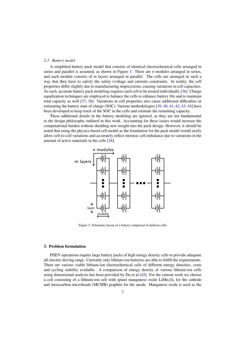
2.3. Battery model

A simplified battery pack model that consists of identical electrochemical cells arranged inseries and parallel is assumed, as shown in Figure 3. There are n modules arranged in series,and each module consists of m layers arranged in parallel. The cells are arranged in such away that they have to satisfy the safety (voltage and current) constraints. In reality, the cellproperties differ slightly due to manufacturing imprecisions, causing variations in cell capacities.As such, accurate battery pack modeling requires each cell to be treated individually [36]. Chargeequalization techniques are employed to balance the cells to enhance battery life and to maintaintotal capacity as well [37, 38]. Variations in cell properties also cause additional difficulties inestimating the battery state of charge (SOC). Various methodologies [39, 40, 41, 42, 43, 44] havebeen developed to keep track of the SOC in the cells and estimate the remaining capacity.

These additional details in the battery modeling are ignored, as they are not fundamentalto the design philosophy outlined in this work. Accounting for these issues would increase thecomputational burden without shedding new insight into the pack design. However, it should benoted that using the physics-based cell model as the foundation for the pack model would easilyallow cell-to-cell variations and accurately reflect intrinsic cell imbalance due to variations in theamount of active materials in the cells [36].

m layers

n modules

layer

module

Figure 3: Schematic layout of a battery comprised of uniform cells

3. Problem formulation

PHEV operations require large battery packs of high energy density cells to provide adequateall-electric driving range. Currently only lithium-ion batteries are able to fulfill the requirements.There are various viable lithium-ion electrochemical cells of different energy densities, costsand cycling stability available. A comparison of energy density of various lithium-ion cellsusing dimensional analysis has been provided by Du et al [45]. For the current work we choosea cell consisting of a lithium-ion cell with spinel manganese oxide LiMn2O4 for the cathodeand mesocarbon microbeads (MCMB) graphite for the anode. Manganese oxide is used as the

7

cathode material, since it is relatively inexpensive, easily disposable, and exhibits good cyclingresistance. The validation of lithium-ion cell with spinel manganese cathode and graphite anodeusing the cell model outlined in Section 2.2 has been provided by Doyle et al [46]. The fixedproperties of the cell are listed in Table 2.

Parameters Valuecathode material Spinel Mn2O4cathode initial stoichiometric parameter (y in LiyMn2O4) 0.2coulombic capacity of cathode material 148 mAh/gdensity of cathode material 4280 kg/m3

volume fraction of inert filler in cathode 0.1bulk diffusivity 10−13m2/ssolid particle radius 2 µmanode material MCMB 2528 graphiteanode initial stoichiometric parameter (x in LixC6) 0.9coulombic capacity of anode 372 mAh/gdensity of anode material 2260 kg/m3

volume fraction of inert material in anode 0.05bulk diffusivity 10−13m2/ssolid particle radius 5 µmelectrolyte material LiPF6 in EC:DMCinitial salt concentration 1000 mol/m3

inert filler material PVDFambient temperature 298 Kcycling rate 1.0 CP-to-N ratio 1.0

Table 2: List of Li-ion cell material properties and fixed parameters [47]

In addition to the fixed variables, six free variables (Table 3) are selected to determine theoptimal cell design and pack configuration that best fulfills the pack requirements. These sixvariables are chosen as they represent design parameters that can be readily manipulated by thebattery manufacturer to determine the battery pack properties. There are other parameters suchas diffusivity and conductivity as well as electrode particle sizes that affect the performance ofthe cell. Our earlier work [25] has shown that in the absence of degradation mechanisms andside reactions, these other variables invariably go to the bounds at optimal cell designs. Theirrelative effects on energy density of the cell have been shown to be less than the morphologicalparameters chosen for this study [22]. Therefore, they are neglected in this study. Among thesix variables, the electrode thicknesses and porosities are morphological parameters that balancethe amount of energy content in the cell with the ion transport requirement. A thicker electrodecontains more active material for the intercalation process, and hence higher energy capacity. Amore porous electrode allows higher rate of ion transport by increasing the effective transport co-efficient. However, it reduces the fraction of charge-storing active materials and overall capacityof the cell. The competing effects of higher energy and higher power results in an optimal celldesign that must reach a compromise between energy and power. The cutoff voltage determinesthe lowest SOC in the cell that can still fulfill the power requirement. The peak power available

8

is dependent on the capacity remaining in the battery and must be accurately determined to avoidover-discharging the battery. While the SOC and cell voltage required to calculate peak powercan be conveniently extracted from the cell model in our framework, a more practical approachwill involve a multi-parameter, model-based method [48] to estimate the peak power. The lastvariable is the number of cells connected in parallel within each module, which also determinesthe maximum current of the pack. The number of modules connected in series is fixed by themaximum voltage of the battery pack, which will be explained in greater detail at the end of thissection.

Parameters Lower bound Upper boundcathode thickness (µm) 40.0 250.0anode thickness (µm) 40.0 250.0cathode porosity (µm) 0.1 0.6anode porosity (µm) 0.1 0.6cut-off voltage (V) 2.6 3.6no. of layers 1 30

Table 3: List of design variables and their ranges

Three key properties of the battery pack are identified as the objective functions to be min-imized, which are the mass, volume and material costs. Each objective can be given as linearfunctions of the design variables:

Mass = nmA∑

j

∑iεi jρil j

Volume = nmA∑

jl j

Cost = nmA∑

j

∑i

biεi jρil j

(5)

where n,m are the number of modules and layers in the battery pack, A is the cross-section ofeach cell, ε, ρ and b are the volume fraction, the mass density and the unit cost [49] of thematerial respectively, and l is the thickness of the cell component. The index j cycles over thecell components, namely the positive electrode, separator, negative electrode, and the currentcollectors, while i cycles over the cell materials. Note that if the materials with higher densityhave higher unit price, then the cost becomes directly correlated with the mass. Reducing thebattery pack mass will invariably reduce the cost as well.

Equations (5) show that the objective functions are linear with respect to the design variables.Minimization of the objective functions without proper consideration of constraints simply re-sults in the trivial solution of all design variables at their lower bounds. Therefore, a usefulbattery pack design requires satisfying appropriate design constraints. These safety and perfor-mance requirements impose limits on how close to the lower bounds the design variables can go.The constraints for our problem are listed in Table 4.

The energy of the battery pack is computed by galvanostatic discharge of the cells at 1Ccycling rate, while the maximum power is the average power available during a 10-second max-imum current pulse at the end of the 1C discharge. The maximum power is computed at thelowest SOC, as this is the point where cell voltage is the lowest. If the battery can meet thepower requirement at the end of discharge, it can meet the power requirement throughout its

9

Pack Cell

Voltage Vpack ≤ 400V

=⇒

n · Vcell,init ≤ 400VVpack ≥ 280V n · Vcell,end ≥ 280V

Current Ipack ≤ 420A m · Icell ≤ 420AEnergy Epack ≥ 12kWh nm · Ecell ≥ 12kWhPower Ppack ≥ 120kW nm · Pcell ≥ 120kWCharge balance Q+ = Q−

Table 4: Conversion of pack-level requirements to cell-level constraints

operation. The 10-second current pulse requirement provides a good estimate of the maximumpower required for vehicle operation, as it mimics the power demand required for acceleratingonto the highway. Based on the constraints outlined in Table 4, the maximum voltage limits thenumber of battery modules connected in series. The maximum voltage in a cell is the open-circuitvoltage at the fully charged state, and the maximum pack voltage divided by this value providesthe number of modules allowed in the battery pack. In this study the number of cells connectedin series is fixed at 99. The minimum voltage is computed at the end of the 10-second maximumcurrent pulse and it sets the limit on the depth of discharge of the cells. Hence, the optimizationproblem can be simplified by replacing the voltage constraints with the fixed number of modulesin the pack and the minimum cell voltage to terminate discharge.

4. Results and discussion

4.1. Discharge profile

A typical discharge profile obtained from the cell-model simulation is shown in Figure 4,which shows both the cell voltage and the current density profiles. The small insert in Figure 4shows the voltage and current profile at the transition between the galvanostatic discharge andpeak power current pulse. The sudden jump in the cell current creates a discontinuity in thevoltage profile. The cell voltage decreases rapidly as the amount of charge is depleted at agreater rate.

The secant method is used to obtain the maximum current during the 10-second pulse. Themaximum current is defined as the largest current required for maintaining the minimum voltageat the end of the pulse. The iterative process for the maximum current computation is shown inFigure 5. The final cell voltage decreases monotonically as the pulse current is increased, andthe negative correlation between the maximum current and the final cell voltage is shown in theinsert.

4.2. Optimization results

As mentioned previously, three different optimization problems are solved using the opti-mization framework to design the PHEV battery pack: 1) to minimize battery mass, 2) to mini-mize battery volume, and 3) to minimize battery material cost. The six design variables are listedin Table 3 and the four constraints are presented in Table 4. To compare the performance ofthe optimized cell designs, three simple initial pack designs are selected. The first two designsfollow the general ‘ad-hoc’ guidelines for cell electrode design; the first one is a power cell withthin electrode and high porosity, and the other is an energy cell with thick electrode and low

10

0 10 20 30 40 50time, min

2.8

3.0

3.2

3.4

3.6

3.8

4.0

cell

pote

ntia

l, V

voltage profile

current profile60

70

80

90

100

110

120

130

curr

ent

dens

ity,

A/m

2

52.5 52.7 52.92.8

3.0

3.2

3.4 Last 20s of discharge

60

80

100

120

Figure 4: Discharge profile for a lithium-ion cell undergoing 1C constant current discharge (main) followed by a 10-second peak power pulse at the end of the discharge (insert)

porosity. The third one is based on the earlier work of cell optimization subjected to a powerconstraint [25]. The optimized cell selected for comparison is designed at the same power-to-energy ratio as specified in the problem definition for the PHEV battery pack. The differencebetween the single cell and pack design philosophy is that single cell optimization is performedat one discharge rate, while the power and energy requirement for the pack design are performedat different discharge rates, resulting in additional constraints in the design problem. The spec-ifications for the three initial designs and their properties are listed in Table 5. All three initialdesigns satisfy the capacity balance requirement imposed on the problem.

Analyses of initial pack designs show that the optimized single cell and power cell designshave similar properties, with the power cell exhibiting slightly better performance. The energycell design is the worst among the three, as its thick electrodes and low porosity result in anexpensive and bulky cell without providing any energy density improvement over the other two.All three initial pack designs require 13 layers of cells in parallel to satisfy the pack constraints.This results in the energy cell designs being the heaviest, most voluminous, and most expensive.

Given that the three separate objective functions are not linear combinations of one another,the optimal design for one objective should not be the optimum for another. Table 5 shows thatthe power cell design performs the best for all three objectives, it is thus not expected to be thetrue optimal design. In addition, while the power requirement of the pack is exceeded, the energycapacity requirement is not fully satisfied by any of the three initial designs. Therefore, furtherimprovement is possible and can be achieved using numerical optimization.

The gradient-free optimization is first carried out to obtain an approximate estimate of the op-timal design and to determine the integer value of cell layers. A representative iteration history ofcost optimization is shown in Figure 6. Note that the ALPSO is a population-based optimizationmethod such that at each iteration, there are multiple design points existing simultaneously. Theplots shown here contain only the design point that best satisfies the design problem criteria ateach iteration, evaluated by the Lagrange function for each particle [28].

Subplots a, b and c in Figure 6 show how the six design variables change during the iteration

11

3160 3162 3164 3166 3168 3170time, sec

2.8

2.9

3.0

3.1

3.2

cell

pote

ntia

l, V

1st iteration

2nd iteration

final iteration

min. voltage

Vmin

potential vs. current

Figure 5: Discharge profiles of the 10-second peak current phase. The secant method is used to determine the maximumcurrent such that the cell potential is exactly at the minimum voltage at the end of the discharge (insert)

while subplot 6d shows the evolution of the objective function (solid line) and the normalizedconstraint values (dashed lines) during the optimization process. The normalized constraint valueis given as a percentage, with 100% and above indicating that the constraint is satisfied. Thecharge balance constraint is an equality constraint that has to be satisfied exactly at all timesand hence is not plotted. The optimization history shown in Figure 6 can be broken down intothree phases. The initial design has high number of layers and this resulted in a high batterycost and extremely high current. The first six iterations reduced the number of layers and hencelowered the current to below the maximum allowed value, however this results in energy andpower requirements being not satisfied. Further adjustment of the design variables in the nextfive iterations converged close to the final cell design, which shows that the energy and powerconstraints are fulfilled exactly, while the maximum current is well above the maximum allowedlevel. Given the competing effects of energy and power in the battery cell, this result is expected,as the optimal cell design would be one that satisfies but does not exceed both requirements.

ALPSO is a stochastic optimization method, hence multiple optimizations runs were per-formed for each optimization problem. The best results are listed in Table 6. Optimizing formass and material costs results in very similar optimal cell designs. In fact, the optimal designobtained for cost minimization has the lowest battery pack mass as well. Given that reductionin battery mass naturally leads to less materials and hence lower cost, this result is not surpris-ing. While the difference between the minimal-mass weight and minimal-cost weight is withinthe convergence tolerance of the optimizer, it also indicates the ALPSO is unable to locate thetrue optima in this situation, such that the final result found for mass minimization problem issub-optimal.

A comparison between Tables 5 and 6 shows decreases of 13.4%, 18.1%, and 17.9% in mass,volume and cost respectively from initial to optimal designs. Compared with the best initial celldesigns, all three optimal designs have thicker electrodes and lower porosities. Therefore eachcell has higher energy density, while still satisfying the power requirement. The energy and

12

power cell energy cell optimized single cellcathode thickness (µm) 129.9 189.8 141.7anode thickness (µm) 80.0 120.0 70.0cathode porosity 0.4 0.2 0.442anode porosity 0.4 0.2 0.322cutoff voltage (V) 3.53 3.63 3.53no of layers 13 13 13mass (kg) 86.89 126.00 87.14volume (dm3) 29.34 39.62 29.52cost ($) 1398 1862 1401energy capacity [≥ 12kWh] 11.9 11.8 11.9maximum current [≤ 420A] 388.0 385.2 389.3peak power [≥ 120kW] 121.5 123.3 121.7

Table 5: Battery cell properties of initial designs

power requirements are satisfied with far fewer cells (9 or 10 layers vs. 13), and hence betteroverall pack properties.

There are some differences between the three optimized designs. The mass and cost mini-mization problems produce optimal cell designs that have thick electrodes, such that the cell hasas much active material for lithium ion intercalation as possible. This is to maximize the energydensity of the cell and to reduce the total amount of materials needed. While cost minimiza-tion problem results in a battery pack lighter than the one obtained from the mass minimizationproblem, the difference is within the convergence tolerance of ALPSO. Volume minimization,on the other hand, produces an optimal cell design that has thinner electrodes with lower porosi-ties. This results in a cell design that has lower gravimetric energy density, but higher volumetricenergy density compared to the designs for the other two problems.

The optimal cell designs are further improved by using SNOPT to refine the continuouscell variables. The gradient-based optimization is initiated at the optimal designs obtained fromALPSO. The number of layers in each module, which is a discrete variable, is fixed at the valuesaround the optimal number of layers obtained via ALPSO, while the gradient-based optimizerfine-tunes the continuous variables. The results obtained using SNOPT are listed in Table 7.Again we notice the similarity between the mass minimization and cost minimization solutions.The two optimal designs are almost identical, and the material cost difference between the two isless than one dollar. The volume minimization problem produces a battery pack with much thin-ner electrodes and lower porosities. Comparing the SNOPT and ALPSO volume minimizationresults, the cathode and anode thicknesses are 21.3% and 25.6% thinner respectively while theporosities are 19.1% and 40.5% less. The number of cells required increases by 20%. The lowelectrode porosity means the cell design is less adequate to handle high discharge rate, howeverthis is alleviated by having a larger number of cells connected in parallel and hence a smallercurrent density through each cell. The SNOPT optimal design has higher mass and material costbut lower volume. While utilizing larger number of cells with lower energy density may seemcounter-intuitive, it demonstrates the ability of the optimizer to drive the design to achieve theobjective, which in this particular instance is to minimize the volume of the pack.

Results in Table 7 show that improvements from gradient-free optmization to gradient-based

13

0 10 20 30 40 50iteration no.

6080

100120140160180200

thic

knes

s (µ

m)

(a)

cathodeanode

0 10 20 30 40 50iteration no.

0.20

0.25

0.30

0.35

0.40

poro

sity

cathodeanode

0 10 20 30 40 50iteration no.

3.35

3.40

3.45

3.50

3.55

3.60

3.65

3.70

cuto

ff v

olt.

(V) cutoff voltage

78910111213141516

no. o

f lay

ers

no. layers(b)

(c)0 10 20 30 40 50

iteration no.900

100011001200130014001500160017001800

cost

(U

S$)

cost

5060708090100110120130140

feas

ibili

ty, %

(d)

peak powermax currentenergy

Figure 6: Iteration history of an optimization to minimize battery cost showing the evolution of: a) electrode thicknesses,b) cutoff-voltage and no of layers, c) electrode porosities, and d) cost and normalized inequality constraint values

optimization results are less than 1% for all three optimization problems. This is mainly due tothe flatness of the design space near the optimum, and there is little gain in pinpointing the exactlocation of the optimal designs, as evidenced by the 8% difference in negative electrode porositybetween ALPSO and SNOPT results. Such differences, however, may become more importantas more details about cell modeling are included. For instance, manganese dissolution rate hasbeen shown to correlate to the interfacial surface area in the porous electrode [50]. Increase incathode porosity will increase interfacial surface area and could potentially cause accelerated celldegradation. Inclusion of additional degradation mechanisms will likely add nonlinearity to thedesign space and further restricts the feasible design regions.

One common problem with gradient-based optimization is that it often converges to localoptimum solutions instead of global best ones. To show that the solutions are indeed globaloptimal and that the design space near the solutions are not dominated by local optima, weobtain the contour plots of the objective functions on the plane that passes through the threeoptimal design points of mass, volume and cost respectively. The plane is obtained by projectingthe design space onto the plane spanned by the coordinates of the three optimal design points.The three optimal points are transformed into the non-dimensional coordinates (0, 0), (1, 0), (0, 1)respectively on the plane. The shaded area on Figure 7 indicates the region where the energy,power, voltage and current requirements are all concurrently satisfied. The blue curve indicates

14

Properties Objective functionMass Volume Cost

mass (kg) 74.97 75.67 74.90volume (dm3) 24.91 24.02 24.48cost ($) 1153 1169 1147cathode thickness (µm) 169.8 141.9 168.8anode thickness (µm) 104.7 86.4 99.8cathode porosity 0.321 0.272 0.305anode porosity 0.314 0.252 0.269cutoff voltage (V) 3.52 3.53 3.53no of layers 9 10 9energy capacity [≥ 12kWh] 12.0 12.0 12.0maximum current [≤ 420A] 398.4 395.0 396.6peak power [≥ 120kW] 120.1 119.9 120.1

Table 6: Preliminary designs after gradient-free optimization. Results shown are the ’best-available’ ones due to stochas-tic nature of ALPSO algorithms.

the narrow band that fulfills the charge balance requirement, while the black lines show thedesign space that satisfies the integer requirement imposed on the number of layers.

In the plots shown in Figure 7, we can see that the objective functions vary smoothly in thefeasible design space. The mass and cost contours vary monotonically in the feasible designspace, while there is a local volume maximum for the volume contour plot. All three opti-mal design points are located on the boundary of the feasible space, again confirming that theconstraints are active in this design problem. The location of the optimal designs are furtherrestricted by the charge capacity equality constraints and the integer requirement on the numberof cell layers. Based on the information available in Figure 7, it is clear that the optimal designsare indeed the best possible designs in the slice of plane shown here. Such information, togetherwith the smoothness of the objective functions, gives us confidence about the global optimalityof the results. The similarity between mass and cost optimal designs can also be explained fromthe contour plots in Figure 7. Comparison of the mass and cost contours reveal that the two ob-jectives are very similar to one another in the given plane. The gradients for both objectives pointin the same x-direction, and in both cases the best objective functions are on the left boundaryof the feasible space. The similarities of the objectives result in mass and cost optimal designsbeing very close to each other in the actual design space.

The optimal cell design for mass minimization problem is compared with the optimal single-cell design from our previous work [25], in which the optimal cell has the maximum energydensity at constrained discharge rates. Comparison to the optimal cell at 1C discharge rate showsthe PHEV pack cell design has thinner electrodes and higher porosities. This is due to the ad-ditional peak power requirement at the end of discharge, which imposes a higher ion transportrequirement. The resulting cell design, while not optimal in term of energy density, is able tomeet both the energy and power requirements simultaneously, which is more important given thevariations in power demand under normal driving conditions.

15

Properties Objective functionMass Volume Cost

mass (kg) 74.77 79.53 75.06volume (dm3) 24.49 23.85 24.37cost ($) 1146 1241 1146cathode thickness (µm) 169.2 111.7 169.4anode thickness (µm) 99.4 64.3 97.5cathode porosity 0.310 0.220 0.300anode porosity 0.270 0.150 0.245cutoff voltage (V) 3.53 3.55 3.54no of layers 9 12 9energy capacity [≥ 12kWh] 12.0 12.0 12.0maximum current [≤ 420A] 395.9 392.5 394.4peak power [≥ 120kW] 119.9 120.1 119.8

Table 7: Refined optimal designs obtained using gradient-based optimizations

Properties Valuesvehicle mass (kg) 1500passenger mass (kg) 150rolling resistance coeff. 0.01drag coefficient 0.30frontal area (m2) 2.0motor efficiency 0.85drivetrain efficiency 0.8generator efficiency 0.85regenerative braking factor 0.1

Table 8: Properties of the vehicle used to complete the driving cycle

4.3. Driving cycle test

While the optimal designs obtained using the aforementioned optimization framework showbetter overall properties than the initial design, it is important to show that they translate to actualperformance advantage in the PHEV operations. We next compare the performance of the batterypacks by simulating discharge using standard federal testing driving cycles. A standard sedanwith the properties listed in Table 8 is used to compute the battery power required to completethe driving cycles. The power needed to follow the driving cycle at any particular time instanceis given as:

Ptot = Pacc + Pdrag + Proll + Pmis (6)

where the total power required is the sum of the power required to overcome aerodynamic forces(Pdrag), rolling resistance(Proll), power miscellaneous systems (Pmis) and to achieve the requiredacceleration (Pacc) of the driving cycle. The miscellaneous power refers to the power requiredfor various auxiliary systems not related to drivetrain and it is given the constant value of 1.0 kW.Using Equation 6, the power required for any driving cycle can be computed.

16

0.2 0.0 0.2 0.4 0.6 0.8 1.0 1.2x-axis

0.2

0.0

0.2

0.4

0.6

0.8

1.0

1.2

y-ax

is charge balance

continuous feasible region

continuous feasible region

integer requirement

73.0

74.0

75.0

76.0

77.0

78.0

79.0 79.0

79.8

mass optcost optvol opt

(a)

0.2 0.0 0.2 0.4 0.6 0.8 1.0 1.2x-axis

0.2

0.0

0.2

0.4

0.6

0.8

1.0

1.2

y-ax

is

charge balance

continuous feasible region

continuous feasible region

integer requirement

23.123.4

23.7

24.0

24.0

24.3 24.324.6

24.6

mass optcost optvol opt

(b)

0.2 0.0 0.2 0.4 0.6 0.8 1.0 1.2x-axis

0.2

0.0

0.2

0.4

0.6

0.8

1.0

1.2

y-ax

is

charge balance

continuous feasible region

continuous feasible region

integer requirement

1120

1140

1160

1180 1200

1220

1240

mass optcost optvol opt

(c)

Grey area represents the feasible design space that satisfies the en-ergy, power and current constraints. The black lines represent in-teger constraint on the number of layers and blue curves representthe part of the design space satisfying charge capacity balance. Thebackgrounds are overlay with the contour plots of a) mass in kg, b)volume in liters, and c) cost in US$.

Figure 7: Contour plots of objective functions on the plane spanning the three optimal design points

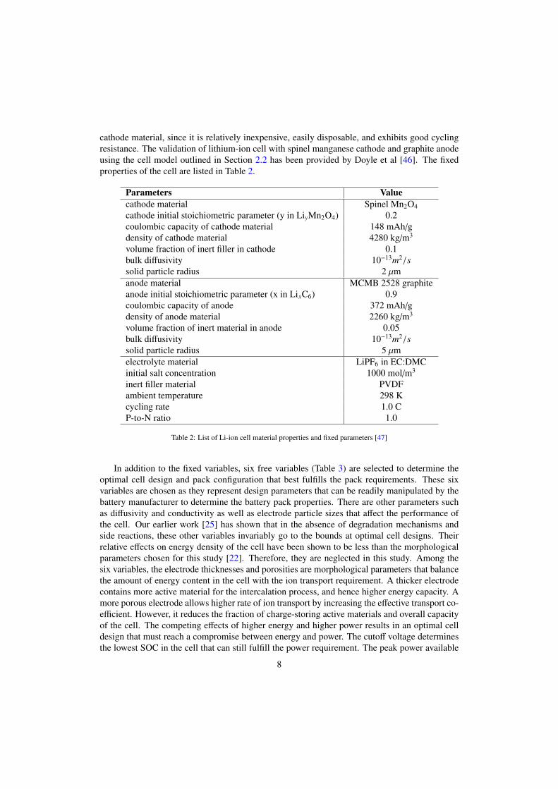
The battery packs are discharged through the three standard federal driving cycles: UDDS,SC03 and US06, with their speed and corresponding power profiles shown in Figure 8. TheUDDS and SC03 cycles both mimic city driving conditions, with SC03 being slightly moreaggressive. US06 simulates highway driving condition. The highway acceleration requirementsimpose higher power demands on the battery, with power demands peaking at 100 kW. Thebattery is discharged from an initial SOC of approximately 0.8 until the minimum voltage of280V is reached and the total distance covered for each of the driving cycle is calculated.

Both the initial design and optimal battery packs are discharged through the simulated drivingcycles. The voltage and SOC profiles of the mimimum mass optimal battery pack and the initialdesign discharged through the simulated US06 driving cycle are shown in Figure 9. The open-curcuit voltage (OCV) curve is plotted on the same figure for comparison. The SOC profileshows that the optimal battery pack lasts longer than the initial design battery pack, resulting in3.5% longer electric range. The initial battery design contains more cells in parallel compared tothe optimal battery pack, therefore each cell is subjected to a smaller current density. This resultsin higher battery pack voltage in the initial design, and less energy lost per cell due to internalresistance. However, the higher energy density of the optimal battery pack cells still result inoverall better performance.

17

0 5 10 15 2005

1015202530

spee

d, m

/s UDDS

010203040

Pow

er, k

W

(a)

0 2 4 6 8 1005

10152025

spee

d, m

/s SC03

01020304050

Pow

er, k

W

(b)

0 2 4 6 8 10time, min

05

10152025303540

spee

d, m

/s US06

020406080100

Pow

er, k

W

(c)

Figure 8: Federal driving cycle speed profiles and the corresponding battery power requirement

Battery designDrive cycle Initial Min. mass Min. volume Min. costUDDS 53.7 km 57.2 km 58.1 km 58.1 kmSC03 48.6 km 52.5 km 53.4 km 53.4 kmUS06 39.7 km 41.1 km 42.1 km 41.8 km

Table 9: All electric driving range for various battery designs

The all electric ranges for various battery pack designs subject to the three driving cycles arelisted in Table 9. For all three driving cycles, the optimal battery pack designs outperform theinitial battery pack designs in terms of all-electric range. The most improvement is in SC03 cycledischarge, with the electric ranges of minimum-volume and minimum-cost battery packs almost10% better than that of the initial design.

While the electric driving range of the optimal battery pack designs show significant improve-ment over the initial design, a better measure of the battery performance would be to measure thedistance travelled per unit of battery performance metric, where the metric is either mass, vol-ume or material cost. Figure 10 compares the performance of the optimal battery designs with thebest initial design. While the initial and optimal designs have similar all-electrice drive range, theoptimal designs clearly have better performance per unit of battery performance metric. On av-erage, the optimal battery packs show 23.1% improvement in distance per unit of battery mass,32.8% improvement in distance per unit volume and 31.4% improvement in distance per unitcost.

Results in Table 9 also shows that the minimum-volume battery pack has the longest elec-tric ranges among the optimal battery pack designs. The disparity between the electric drivingranges of the various optimal battery packs demonstrates that while the battery packs satisfysimiliar energy and power requirements, the performance is dependent on the driving cycle, orcontrol variables governing the discharge of the battery. This points to the possible advantages of

18

0 5 10 15 20 25 30time, min

0.0

0.1

0.2

0.3

0.4

0.5

0.6

0.7

0.8SO

C

SOC

optimalinitial

260

280

300

320

340

360

380

400

volt

age,

Vvoltage

OCV

init. range: 39.7 kmopt. range: 41.1 km

Figure 9: Comparison of the voltage and SOC profiles of the initial design and minimum-mass optimal battery packdischarged through the simulated US06 driving cycle

UDDS SC03 US060.20.30.40.50.60.70.8

km/k

g

(a)

mass optinit

UDDS SC03 US060.5

1.0

1.5

2.0

2.5

km/l

(b)

vol optinit

UDDS SC03 US060.000.010.020.030.040.050.06

km/$

(c)

cost optinit

Figure 10: Comparison of battery performance between initial and optimal designs using driving cycle data

19

performing a design-control coupled optimization. In addition, we only consider the all-electricoperating mode of the PHEV drive and not the overall performance of the PHEV. The problemdefinition is limited to minimizing the properties of the battery pack, and this allows decouplingof the battery from other drivetrain components. To truly optimize the operation of the PHEV,the hybrid mode, during which both engine and electric power are in use, needs to be consideredas well. The degree of hybridization in the PHEV, which is the ratio of electric motor power tothe total drivetrain power, is shown to affect the optimality of the drivetrain components perfor-mance [51]. Therefore, the overall hybridization scheme of a PHEV is defined by the battery,electric motor and internal combustion engine collectively [14]. Inclusion of various componentsalso necessitates the coupling of power control strategies with design parameters to determine theoptimal performance. Kim and Peng [18] has shown that the ”power management and design”optimization showed a 17% improvement in fuel economy over ”power management only” re-sults. Consideration of the engine and electric motor sizes could allow for battery design that bestmeets the peak power demand during climbing and acceleration, and keeps the engine operationat maximum efficiency.

5. Conclusions

This work outlines a methodology to perform battery design optimization by coupling anumerical optimization framework with a physics-based electrochemical cell model. Given thenonlinear and mixed-integer nature of the optimization problem, a hybrid optimization approachwas developed. A gradient-free optimizer is first used to obtain an approximate estimate of theoptimal design and to obtain the optimal integer design variables. The design is then furtherrefined using the gradient-based optimization. Such a framework is very useful to obtain thebest possible initial designs, from which further refinement can be carried out by accounting foradditional details such as degradation mechanisms and manufacturing constraints. Comparisonsbetween the initial and optimal designs show overall improvements of 13.9%, 18.7% and 18.0%in battery mass, volume and cost, respectively. The optimal designs also perform better in realdrive cycle simulations. The improvements in battery pack properties can be translated to 23.1%increase in distance traveled per unit mass, 32.8% increase in distance per unit volume, and31.4% increase in distance per unit cost. The electrochemical cell in this case is assumed to beideal and additional capacity fade mechanisms should be considered in the future.

Acknowledgements

The present efforts were supported by the General Motors and University of Michigan Ad-vanced Battery Coalition for Drivetrains (ABCD). All computations were performed on theFLUX high-performance computing network, sponsored by the College of Engineering, Uni-versity of Michigan.

List of Symbols

Electrochemistry variablesa interfacial surface areaA cross-section area of an electrochemical cell

20

b material unit costc salt concentration in electrolytecs salt concentration in solid matrixD diffusion coefficient of electrolyteDs diffusion coefficient of solid matrixf ± mean molar activity coefficient of electrolyteF Faraday’s constantin transfer current density at the surface of active materialio exchange current densityi2 current density in electrolytel thicknessm number of electrochemical cell in paralleln number of electrochemical cell in seriesQ charge capacityR universal gas constantT temperatureU surface overpotentialαa, αc anodic and cathodic transfer quotientε volume fractionκ ionic conductivity in electrolyteσ ionic conductivity in solid matrixΦ1 potential in solid matrixΦ2 potential in electrolyteρ material densitySubscriptso initial state values value in solid matrix+ positive electrode− negative electrodeOptimization variablesA Jacobian of constraints w.r.t. design variablesc j inequality constraintsck equality constraintsg gradient vector of objective w.r.t. design variablespi best position of the ith particlepg global best positionr1, r2 random numbers between 0 and 1s solution to the quadratic subproblem in SQPV velocity of particle in design spacew0 inertia weight in ALPSOw1, w2 confidence parameters in ALPSOW estimate of second-order derivatives in SQPx position of particle in design space∆t time step value in ALPSO, normally taken to be 1

21

References

[1] M. Ehsani, Y. Gao, J. M. Miller, Hybrid electric vehicles: architecture and motor drives, Proceedings of the IEEE95 (4) (2007) 719–728.

[2] B. Scrosati, J. Garche, Lithium batteries: status, prospects and future, J Power Sources 195 (9) (2010) 2419–2430.[3] C. Sandy Thomas, Transportation options in a carbon-constrained world: Hybrids, plug-in hybrids, biofuels, fuel

cell electric vehicles, and battery electric vehicles, Int J Hydrogen Energ 34 (23) (2009) 9279–9296.[4] M. Alamgir, A. M. Sastry, Efficient batteries for transportation applications, SAE Paper (2008) 21–0017.[5] M. Doyle, T. F. Fuller, J. Newman, Modeling of galvanostatic charge and discharge of the lithium/polymer/insertion

cell, J Electrochem Soc 140 (6) (1993) 1526–1533.[6] M. Valvo, F. E. Wicks, D. Robertson, S. Rudin, Development and application of an improved equivalent circuit

model of a lead acid battery, in: Energy Conversion Engineering Conference, 1996. IECEC 96., Proceedings of the31st Intersociety, Vol. 2, IEEE, 1996, pp. 1159–1163.

[7] B. Yann Liaw, G. Nagasubramanian, R. G. Jungst, D. H. Doughty, Modeling of lithium ion cells - a simpleequivalent-circuit model approach, Solid State Ionics 175 (1) (2004) 835–839.

[8] W. Gu, C. Wang, B. Liaw, The use of computer simulation in the evaluation of electric vehicle batteries, J PowerSources 75 (1) (1998) 151–161.

[9] M. W. Verbrugge, R. S. Conell, Electrochemical and thermal characterization of battery modules commensuratewith electric vehicle integration, J Electrochem Soc 149 (1) (2002) A45–A53.

[10] V. Ramadesigan, P. W. Northrop, S. De, S. Santhanagopalan, R. D. Braatz, V. R. Subramanian, Modeling andsimulation of lithium-ion batteries from a systems engineering perspective, J Electrochem Soc 159 (3) (2012)R31–R45.

[11] A. Cooper, Development of a lead-acid battery for a hybrid electric vehicle, J Power Sources 133 (1) (2004) 116–125.

[12] B. Y. Liaw, M. Dubarry, From driving cycle analysis to understanding battery performance in real-life electrichybrid vehicle operation, J Power Sources 174 (1) (2007) 76–88.

[13] M. Dubarry, V. Svoboda, R. Hwu, B. Y. Liaw, A roadmap to understand battery performance in electric and hybridvehicle operation, J Power Sources 174 (2) (2007) 366–372.

[14] S. K. Shahi, G. G. Wang, L. An, E. Bibeau, Z. Pirmoradi, Using the pareto set pursuing multiobjective optimizationapproach for hybridization of a plug-in hybrid electric vehicle, J Mech Design 134 (2012) 094503–1–6.

[15] X. Wu, B. Cao, X. Li, J. Xu, X. Ren, Component sizing optimization of plug-in hybrid electric vehicles, ApplEnerg 88 (3) (2011) 799–804.

[16] Y.-H. Hung, C.-H. Wu, An integrated optimization approach for a hybrid energy system in electric vehicles, ApplEnerg 98 (2012) 479–490.

[17] Y. Zou, F. Sun, X. Hu, L. Guzzella, H. Peng, Combined optimal sizing and control for a hybrid tracked vehicle,Energies 5 (11) (2012) 4697–4710.

[18] M.-J. Kim, H. Peng, Power management and design optimization of fuel cell/battery hybrid vehicles, J PowerSources 165 (2) (2007) 819–832.

[19] K. Darcovich, E. Henquin, B. Kenney, I. Davidson, N. Saldanha, I. Beausoleil-Morrison, Higher-capacity lithiumion battery chemistries for improved residential energy storage with micro-cogeneration, Appl Energ 111 (0) (2013)853 – 861. doi:http://dx.doi.org/10.1016/j.apenergy.2013.03.088.

[20] J. Newman, Optimization of porosity and thickness of a battery electrode by means of a reaction-zone model, JElectrochem Soc 142 (1) (1995) 97–101.

[21] C. Fellner, J. Newman, High-power batteries for use in hybrid vehicles, J Power Sources 85 (2) (2000) 229–236.[22] W. Du, A. Gupta, X. Zhang, A. M. Sastry, W. Shyy, Effect of cycling rate, particle size and transport properties on

lithium-ion cathode performance, Int J Heat Mass Trans 53 (17) (2010) 3552–3561.[23] V. Ramadesigan, R. N. Methekar, F. Latinwo, R. D. Braatz, V. R. Subramanian, Optimal porosity distribution for

minimized ohmic drop across a porous electrode, J Electrochem Soc 157 (12) (2010) A1328–A1334.[24] S. Golmon, K. Maute, M. L. Dunn, Multiscale design optimization of lithium ion batteries using adjoint sensitivity

analysis, Int J Numer Methods Eng 92 (5) (2012) 475–494.[25] N. Xue, W. Du, A. Gupta, W. Shyy, A. M. Sastry, J. R. R. A. Martins, Optimization of a single lithium-ion battery

cell with a gradient-based algorithm, J Electrochem Soc 160 (8) (2013) A1071–A1078.[26] D. Sumitava, P. W. Northrop, V. Ramadesigan, V. R. Subramanian, Model-based simultaneous optimization of

multiple design parameters for lithium-ion batteries for maximization of energy density, J Power Sources 227(2013) 161–170.

[27] A. B. Lambe, J. R. R. A. Martins, Extensions to the design structure matrix for the description of multidisci-plinary design, analysis, and optimization processes, Struct Multidiscip O 46 (2012) 273–284. doi:10.1007/

s00158-012-0763-y.[28] P. W. Jansen, R. E. Perez, Constrained structural design optimization via a parallel augmented Lagrangian particle

22

swarm optimization approach, Comput Struct 89 (2011) 1352–1366. doi:10.1016/j.compstruc.2011.03.

011.[29] R. E. Perez, P. W. Jansen, J. R. R. A. Martins, pyOpt: a Python-based object-oriented framework for nonlinear

constrained optimization, Struct Multidiscip O 45 (1) (2012) 101–118. doi:10.1007/s00158-011-0666-3.[30] P. Gill, W. Murray, M. Saunders, SNOPT: An SQP algorithm for large-scale constraint optimization, SIAM J

Optimiz 12 (4) (2002) 979–1006.[31] J. Nocedal, S. J. Wright, Numerical Optimization, 2nd Edition, Springer, 2006.[32] J. R. R. A. Martins, P. Sturdza, J. J. Alonso, The complex-step derivative approximation, ACM T Math Software

29 (3) (2003) 245–262. doi:10.1145/838250.838251.[33] K. Thomas, J. Newman, R. Darling, Mathematical modeling of lithium batteries, Advances in Lithium-ion Batteries

(2002) 345–392.[34] J. Newman, K. E. Thomas-Alyea, Electrochemical Systems, Wiley-Interscience, 2004.[35] V. D. Bruggeman, Berechnung verschiedener physikalischer konstanten von heterogenen substanzen. i. dielek-

trizitatskonstanten und leitfahigkeiten der mischkorper aus isotropen substanzen, Annalen der Physik 416 (7)(1935) 636–664.

[36] M. Dubarry, N. Vuillaume, B. Y. Liaw, From single cell model to battery pack simulation for Li-ion batteries, JPower Sources 186 (2) (2009) 500–507.

[37] Y.-S. Lee, M.-W. Cheng, Intelligent control battery equalization for series connected lithium-ion battery strings,Industrial Electronics, IEEE Transactions on 52 (5) (2005) 1297–1307.

[38] S. W. Moore, P. J. Schneider, A review of cell equalization methods for lithium ion and lithium polymer batterysystems, SAE Publication (2001) 01–0959.

[39] C. Hu, B. D. Youn, J. Chung, A multiscale framework with extended Kalman filter for lithium-ion battery SOC andcapacity estimation, Appl Energ 92 (0) (2012) 694 – 704. doi:http://dx.doi.org/10.1016/j.apenergy.

2011.08.002.[40] H. Dai, X. Wei, Z. Sun, J. Wang, W. Gu, Online cell SOC estimation of Li-ion battery packs using a dual time-scale

Kalman filtering for EV applications, Appl Energ 95 (0) (2012) 227 – 237. doi:http://dx.doi.org/10.1016/j.apenergy.2012.02.044.

[41] L. Zhong, C. Zhang, Y. He, Z. Chen, A method for the estimation of the battery pack state of charge based onin-pack cells uniformity analysis, Appl Energ 113 (0) (2014) 558 – 564. doi:http://dx.doi.org/10.1016/

j.apenergy.2013.08.008.[42] R. Xiong, F. Sun, Z. Chen, H. He, A data-driven multi-scale extended kalman filtering based parameter and state

estimation approach of lithium-ion olymer battery in electric vehicles, Appl Energ 113 (0) (2014) 463 – 476.doi:http://dx.doi.org/10.1016/j.apenergy.2013.07.061.

[43] Y. Xing, W. He, M. Pecht, K. L. Tsui, State of charge estimation of lithium-ion batteries using the open-circuitvoltage at various ambient temperatures, Appl Energ 113 (0) (2014) 106 – 115. doi:http://dx.doi.org/10.1016/j.apenergy.2013.07.008.

[44] Y. Zheng, M. Ouyang, L. Lu, J. Li, X. Han, L. Xu, H. Ma, T. A. Dollmeyer, V. Freyermuth, Cell state-of-chargeinconsistency estimation for LiFePO4 battery pack in hybrid electric vehicles using mean-difference model, ApplEnerg 111 (0) (2013) 571 – 580. doi:http://dx.doi.org/10.1016/j.apenergy.2013.05.048.

[45] W. Du, N. Xue, A. M. Sastry, J. R. Martins, W. Shyy, Energy density comparison of Li-ion cathode materials usingdimensional analysis, J Electrochem Soc 160 (8) (2013) A1187–A1193.

[46] M. Doyle, J. Newman, A. S. Gozdz, C. N. Schmutz, J.-M. Tarascon, Comparison of modeling predictions withexperimental data from plastic lithium ion cells, J Electrochem Soc 143 (6) (1996) 1890–1903.

[47] M. Park, X. Zhang, M. Chung, G. B. Less, A. M. Sastry, A review of conduction phenomena in Li-ion batteries, JPower Sources 195 (24) (2010) 7904–7929.

[48] F. Sun, R. Xiong, H. He, W. Li, J. E. E. Aussems, Model-based dynamic multi-parameter method for peak powerestimation of lithiumion batteries, Appl Energ 96 (0) (2012) 378 – 386. doi:http://dx.doi.org/10.1016/j.apenergy.2012.02.061.

[49] K. G. Gallagher, D. Dees, P. Nelson, Phev battery cost assessment (2011).[50] D. H. Jang, Y. J. Shin, S. M. Oh, Dissolution of spinel oxides and capacity losses in 4 V Li/LixMn2O4 cells, J

Electrochem Soc 143 (7) (1996) 2204–2211.[51] J. Larminie, J. Lowry, Electric vehicle technology explained, Wiley Online Library, 2012.

23