Progress In Electromagnetics Research M, Vol. 31, 103–116, 2013

DESIGN OF A LOW SIDELOBE 4D PLANAR ARRAYINCLUDING MUTUAL COUPLING

Quanjiang Zhu, Shiwen Yang*, Ruilin Yao, and Zaiping Nie

School of Electronic Engineering, University of Electronic Science andTechnology of China (UESTC), Chengdu 611731, China

Abstract—An efficient approach is presented for the design of alow sidelobe four-dimensional (4D) planar antenna array, taking intoaccount mutual coupling and platform effect. The approach is basedon the combination of the active element patterns and the differentialevolution (DE) algorithm. Different from linear and circular arrays, themutual coupling compensation in a planar array is more complicatedsince it requires numerous data of the active element patterns indifferent azimuth planes. In order to solve this problem, a usefulinterface program is developed to get these data from commercialsoftware HFSS automatically. Also different from conventional lowsidelobe arrays with tapered amplitude excitations, the low sidelobein the 4D array is realized using time-modulation technique underuniform static amplitude and phase conditions. The DE algorithmis used to optimize the time sequences which are equivalent to thecomplex excitations in conventional arrays. Both computed resultsand simulated results in HFSS show that a −30 dB sidelobe patterncan be synthesized in a 76-element planar array with an octagonalground plane and a radome, thus verifying the proposed approach.

1. INTRODUCTION

Four-dimensional (4D) antenna arrays, which are also termed as timemodulated arrays in literature [1–8], are formed by introducing afourth dimension, time, into conventional antenna arrays operatingin the 3-dimensional space. As compared to conventional arrays,the 4D arrays have much more flexibility in pattern synthesis, dueto the additional degree of design freedom, time. For example,low sidelobe level (SLL) patterns can be synthesized in 4D arrays

Received 22 February 2013, Accepted 27 May 2013, Scheduled 30 May 2013* Corresponding author: Shiwen Yang (swnyang@uestc.edu.cn).

104 Zhu et al.

with uniform static amplitude and phase excitations. In the pastdecade, many studies have been carried out to synthesize desiredpatterns and suppress the sideband level (SBL) in 4D linear andplanar arrays using various optimization algorithms [3–11]. Recently,some studies show that 4D arrays have promising potentials forsome practical applications, such as harmonic beamforming withoutphase shifting [12, 13], direction finding [14, 15], monopulse radardesign [16, 17], adaptive nulling [18, 19], and directional modulationfor secure communication [20]. All these distinct advantages in 4Darrays are based on the exploitation and utilization of the sidebandsignals caused by time modulation.

This paper focuses on the pattern synthesis of 4D planar arrays,taking into account the mutual coupling and platform effect. Althoughthe pattern synthesis of 4D planar arrays has been reported in [9–11] where isotropic elements are used, the mutual coupling effect hasnot been addressed. Mutual coupling among antenna elements inantenna arrays can strongly affect the radiation pattern, especiallyin small- and medium-sized arrays [21]. Many efforts have been madeto compensate for the mutual coupling effect through the couplingimpendence matrix combining numerical computation technique (e.g.,method of moments) [22–24]. They are very efficient descriptions ofthe coupling effect for linear and circular arrays with simple elements.However, the approach is no longer adequate for a planar array withtens of complex elements and a platform, as the computation of thecoupling matrix is a very heavy burden.

The active element pattern method is a very simple but powerfultool to account for the mutual coupling and platform effect [25–29].The active element pattern of an array is defined as the radiationpattern of the array when a single radiating element is driven andall the other elements are terminated with matched loads. The activeelement patterns have a specific relationship with mutual impedancematrices in array antennas. The later can be determined fromthe former [30, 31]. The radiation pattern of a fully excited arraycan be expressed as the sum of the active element patterns scaledcorresponding complex excitations, without taking into account thearray factor. Since the active element patterns are produced inthe presence of the mutual coupling and platform effects, the arrayresponse includes mutual coupling and platform effects. The activeelement pattern can be obtained by either measurement or full-wavesimulation of the array. Of course, the latter is more preferable formost antenna engineers nowadays, as this task can be fulfilled easilyby several commercial simulation solvers, such as HFSS and CST. Afterthe data of active element patterns are obtained and stored, the pattern

Progress In Electromagnetics Research M, Vol. 31, 2013 105

synthesis can be performed using global optimization algorithms (e.g.,differential evolution [3, 32–34]).

The paper is organized as follows. In Section 2, a 76-elementprinted dipole planar array is presented. Simulated results show thatthe array elements can operate from 2.0 GHz to 4.0 GHz, with an activeVSWR of less than 1.5. In Section 3, some mathematical formulationsof 4D arrays are presented, and field computation disciplines indifferent coordinate systems are explained. Then an effective procedureis introduced to automatically acquire the data of active elementpatterns of individual elements in different azimuth planes. Combiningthe stored active element pattern data, the DE algorithm is used tooptimize the time sequences for synthesizing a low sidelobe pattern.In Section 5, some numerical results are reported to demonstrate theeffectiveness of the proposed pattern synthesis approach, includingcomputed patterns and simulated patterns by HFSS. Finally, someconclusions are drawn.

2. DESIGN OF THE PLANAR ARRAY

The main difference between 4D arrays and conventional arrays lies inthe feeding network. Different from conventional low SLL array withtapered amplitude excitations, the 4D planar array presented in thispaper is time-modulated to achieve equivalent amplitude weighting atthe center frequency and both amplitude and phase weighting at thesideband frequencies. In this paper, commercial software HFSS is usedto design and simulate the 4D planar arrays [35].

Figure 1 shows a 4D planar array consisting of 76 printed dipoles.

Printed dipole

Figure 1. Geometry of the 76-element planar array with an octagonalground plane.

106 Zhu et al.

For simplicity, the feeding network including the RF switches is notsimulated in HFSS, since it does not affect of the radiation pattern ofthe 4D array. The elements are uniformly laid out in a rectangularlattice in the XY plane, with an inter-element separation of halfwavelength at 2.5 GHz. The planar array is covered by a radome andbacked on an octagonal ground plane.

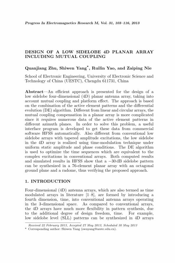
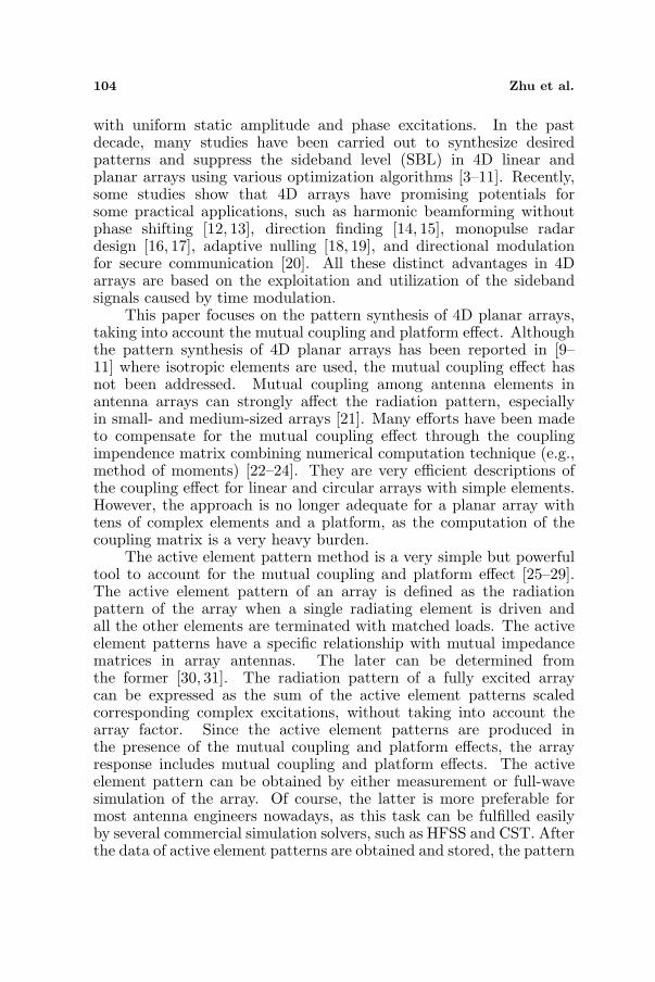
Figure 2 illustrates the simulated active VSWR of an antennaelement in an infinite array where master and slave boundaries areused. Figure 3 shows the simulated active VSWRs of different elementsin the 76-element array (the No. of antenna elements is referred toFigure 6). As can be seen, the array elements can be used to operatefrom 2.0 GHz to 4.0GHz (VSWR < 1.5). The VSWRs of the elementsnear the center of the array (e.g., No. 1, 2 and 6) are almost thesame as that of a single element in an infinite array. This is due tothat mutual coupling effect is most significant between neighboringelements, and the center elements experience approximately the sameelectromagnetic environment as an element in an infinite array. Theactive VSWRs of the elements near the edges of the array (e.g., No. 4and 5) deteriorate, since they experience a different electromagneticcoupling environment as the elements near the center. The goodimpendence matching performance is necessary to ensure that thearray has a higher realized gain, whose definition includes the effectof reflected power [25].

1.5 2.0 2.5 3.0 3.5 4.0 4.51

2

3

4

5

Frequency(GHz)

Act

ive V

SW

R

Figure 2. The active VSWR ofan element in an infinite array.

1.5 2.0 2.5 3.0 3.5 4.0 4.51

2

3

4

Act

ive V

SW

R

Frequency(GHz)

Element No.1

Element No.2

Element No.3

Element No.4

Element No.5

Element No.6

Figure 3. The active VSWRsof different elements in the 76-element planar array when allelements are uniformly excited.

As the geometry of the 76-element array is almost symmetricalwith respect to the XZ and Y Z planes, both the two planes areset as symmetry boundaries. The 76-element array is reduced intoa 19-element subarray, as shown in Figure 4. Assigning symmetry

Progress In Electromagnetics Research M, Vol. 31, 2013 107

Figure 4. Geometry of the19-element subarray obtained bysplitting the 76-element arrayfrom the XZ and Y Z plane.

-180 -120 -60 0 60 120 180-60

-50

-40

-30

-20

-10

0

N

orm

aliz

ed pow

er pattern

(dB

)

θ (degree)

76-element array19-element subarray

Figure 5. Comparison of theradiation patterns of the 76-element array and the 19-elementsubarray in ϕ = 10◦ plane.

boundaries will reduce the computation burden significantly for thepattern synthesis in the following parts. To validate the model, theradiation patterns of the full array shown in Figure 1 and the subarrayshown in Figure 4 are compared. Figure 5 illustrates the comparisonof the radiation patterns of the 76-element array and the 19-elementsubarray in ϕ = 10◦ plane. The pattern of the subarray with symmetryboundaries matches well with the pattern of the full array.

3. PATTERN SYNTHESIS APPROACH

3.1. Mathematical Formulation of 4D Arrays

In this paper, the 4D planar array is supposed to operate at the centerfrequency f0 = 2.5GHz, with uniform static amplitude and phaseexcitations. In order to synthesize a low SLL pattern, the array is time-modulated by RF switches and its time sequences will be optimized inthe subsequent part. The time modulation period is set as Tp, with atime modulation frequency fp = 1/Tp (fp ¿ f0, the radiation patternis independent of fp). For simplicity, the time modulation scheme ofpulse shifting proposed by Poli and Rocca is adopted [36], which isan appropriate trade-off between the flexibility and complexity of thetime sequences. The periodic switch on-off time function Ui(t) for theith element can be given by

Ui(t) ={

1 ti ≤ t ≤ ti + τi

0 others (1)

where 0 ≤ ti ≤ 1 and 0 ≤ τi ≤ 1. ti and τi denote the switch-on timeand on-off time interval for the ith element, respectively. Both of them

108 Zhu et al.

are normalized values.The time modulation in 4D arrays can bring on equivalent

amplitude excitations at the center frequency, and both amplitudeand phase excitations at the sideband frequencies in a time-averagesense. Using Fourier series decomposition approach [2], the equivalentcomplex excitations for the ith element at the center frequency f0 andthe first order sideband frequency f0 + fp are expressed as

w0(i) = τi

w1(i) = τi sin c(πτi) · e−jπ(2ti+τi)(2)

where w0(i) and w1(i) denote the complex excitations at f0 and f0+fp,respectively. Since the higher order sideband levels of 4D antennaarrays with pulse shifting are usually much lower than that of thefirst sideband, only the equivalent complex excitations at the centerfrequency and the first sideband are considered in this paper.

3.2. Coordinate System in HFSS

By the principle of superposition, the radiation vector field of thefully excited array can be expressed as the superposition of the activeelement patterns scaled by corresponding complex excitations, givenby

Emθ (θ, ϕ) =

N∑

i=1

wm(i) ·Eθ(i, θ, ϕ),

Emϕ (θ, ϕ) =

N∑

i=1

wm(i) ·Eϕ(i, θ, ϕ)

(3)

y

x

z

1 2 3 4 5 y

x

z

θ

ϕ6 7 8 9 10

11 12 13 14

15

19

1716

18

ϕ

( , , ) E iθ θ ϕ

( , , ) E i θ ϕ

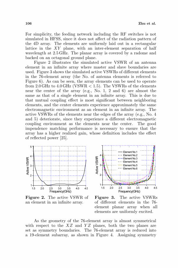
Figure 6. The coordinate system for the 19-element subarray.

Progress In Electromagnetics Research M, Vol. 31, 2013 109

where Emθ (θ, ϕ) and Em

ϕ (θ, ϕ) are the θ- and ϕ-components ofthe total vector field in the mth sideband frequency (m = 0 or 1,corresponding to f0 and f0 + fp). N = 19 is the number of elements inthe subarray. Eθ(i, θ, ϕ) and Eϕ(i, θ, ϕ) are the θ- and ϕ-componentsof the active element pattern produced by the ith element. wm(i) isthe equivalent excitation of the ith element, which is calculated by (2).Quantities in boldface type are vectors, and the active element patternscontain both magnitude and phase data. As the active element patternrepresents the pattern radiated by the entire array when only oneelement is directly excited and the other elements are parasiticallyexcited by the active element, it includes the effects of mutual couplingand the platform.

The total field pattern radiated by the fully excited array can beaccurately expressed combining the two parts, E θ and Eϕ, given by

|Emtotal(θ, ϕ)| =

√∣∣Emθ (θ, ϕ)

∣∣2 +∣∣Em

ϕ (θ, ϕ)∣∣2 (4)

In general, the co-polarization and cross-polarization patterns arepaid more attention to, which can be expressed as

Eco-pol =Eθ cos(ϕ)−Eϕ sin(ϕ), Ecross-pol =Eθ sin(ϕ)+Eϕ cos(ϕ) (5)

Based on the simulation of the array in HFSS, the cross-polarizationcomponent level is −40 dB lower than the co-polarization componentlevel, which implies that the co-polarization field pattern can beexpressed approximately with the total field pattern. In the following,all the radiation patterns refer to the total field patterns.

3.3. Acquisition of Active Element Patterns

The key problem of the active element pattern method is how to acquirethe active pattern data in an easy way. For the aforementioned arraywith 19 elements, even if the array response is computed at the azimuthplanes from ϕ = 0◦ to 90◦ at a step of 10◦, there are still 19 × 10sets of data recording the amplitude and phase of both the Eθ and Eϕ

components. Obviously, it is a rather cumbersome task to obtain thesedata after changing the port excitations in HFSS manually.

In order to solve this problem, an effective procedure has beendeveloped to acquire the active element pattern data, as shown inFigure 7, with the help of the .vbs interface program readable by HFSS.With the procedure the 19 elements are excited individually in turnwith unity terminal voltage and zero phase while the other elements areunder matched load conditions. The .vbs file can be used to controlthe HFSS, change the port excitations and export the pattern dataautomatically. In order to reduce the numerical computation burden,

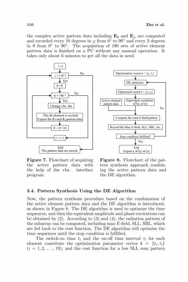
110 Zhu et al.

the complex active pattern data including Eθ and Eϕ are computedand recorded every 10 degrees in ϕ from 0◦ to 90◦ and every 2 degreesin θ from 0◦ to 90◦. The acquisition of 190 sets of active elementpattern data is finished on a PC without any manual operation. Ittakes only about 6 minutes to get all the data in need.

Change vbs. file

The i th element is excited. Export the E and E pattern data

i =1

i <=19 ?

=0

Yes

No

<=90 ?

Yes

= +10

i= i+1

No

End The pattern data are stored.

ϕ

ϕ

ϕ θ

ϕ ϕ

Figure 7. Flowchart of acquiringthe active pattern data withthe help of the vbs. interfaceprogram.

Active element pattern data

Compute the total E-field pattern

DE optimizer

Record the Max E-field, SLL, SBL, etc.

Stop condition fulfilled?

Optimization vector t = {ti, i}

Optimized vector t = {ti, i}

Equivalent excitation w0(i), w

1(i)

End Export t, w

0(i), w

1(i)

No

Yes

τ

τ

Figure 8. Flowchart of the pat-tern synthesis approach combin-ing the active pattern data andthe DE algorithm.

3.4. Pattern Synthesis Using the DE Algorithm

Now, the pattern synthesis procedure based on the combination ofthe active element pattern data and the DE algorithm is introduced,as shown in Figure 8. The DE algorithm is used to optimize the timesequences, and then the equivalent amplitude and phase excitations canbe obtained by (2). According to (3) and (4), the radiation pattern ofthe subarray can be computed, including max E-field, SLL, SBL, whichare fed back to the cost function. The DE algorithm will optimize thetime sequences until the stop condition is fulfilled.

The switch-on time ti and the on-off time interval τi for eachelement constitute the optimization parameter vector t = {ti, τi}(i = 1, 2, . . . , 19), and the cost function for a low SLL sum pattern

Progress In Electromagnetics Research M, Vol. 31, 2013 111

is constructed and given by

f(t)=α1 ·max(Etotal(t)) |f0+α2 · SLL(t) |f0+α3 · SBL(t)∣∣f0+fp (6)

where max(Etotal) is the maximum amplitude of the total E-field at f0,which is related to the gain of the array. SLL is the computed sidelobelevel at f0, and SBL is the computed sideband level at f0 + fp. α1, α2,and α3 are corresponding weighting factors for each term.

Although the pattern synthesis approach is presented for 4Darrays, it can be slightly modified and applied to conventional arraysby ignoring the sideband radiation pattern (the term of SBL).

4. NUMERICAL RESULTS

The optimization target is to synthesize a −30 dB SLL pattern at thecenter frequency f0, while suppressing the SBL to be as low as possible.The search ranges for the switch-on time ti (i = 1, 2, . . . , 19) and on-off time interval τi are chosen as [0, 1.0] and [0.1, 1.0], respectively.

Figure 9 shows the normalized far field patterns in differentazimuth planes at f0. Due to the additional degree of design freedomin 4D arrays, the optimized SLL can be lowered to −30.0 dB. It isknown that the SLL of a conventional uniformly excited planar arraywithout time modulation is about −16 dB. Thus, the time modulationin 4D arrays achieves a SLL reduction of about −14 dB. Figure 10illustrates the pattern of the first sideband signal. It is seen that theSBL is suppressed to −28.5 dB. The corresponding pulse shifting timesequences are plotted in Figure 11 where the gray part means that theswitches are ON.

0 10 20 30 40 50 60 70 80 90-50

-40

-30

-20

-10

0= 50°

= 60°

= 70°

= 80°

= 90°

Norm

aliz

ed pow

er pattern

(dB

)

θ (degree)

, ϕ = 0 °

=10 °

= 20 °

= 30 °

= 40 °

0

, ϕ

0, ϕ

0

, ϕ0

, ϕ0

f

f

f

f

f

, ϕ0

, ϕ

0, ϕ

0

, ϕ0

, ϕ0

f

f

f

f

f

Figure 9. Computed radiationpattern at the center frequencyfor the 19-element subarray withtime-modulation.

0 10 20 30 40 50 60 70 80 90-50

-40

-30

-20

-10

0

= 50°

= 60°

= 70 °

= 80°

= 90°

Norm

aliz

ed pow

er pattern

(dB

)

θ (degree)

0°

= 10°

= 20°

= 30°

= 40°

f + f = 0 p, ϕ

0f + f p, ϕ

0f + f p, ϕ

0f + f p, ϕ

0f + f p, ϕ

0f + f p, ϕ

0f + f p, ϕ

0f + f p, ϕ

0f + f p, ϕ

0f + f p, ϕ

Figure 10. Computed radiationpattern at the first sideband fre-quency for the 19-element subar-ray with time-modulation.

112 Zhu et al.

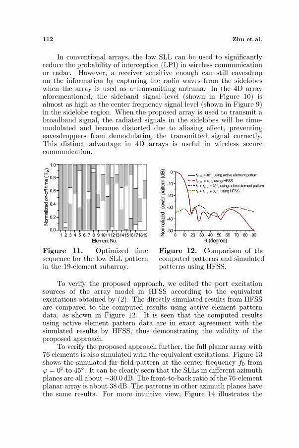
In conventional arrays, the low SLL can be used to significantlyreduce the probability of interception (LPI) in wireless communicationor radar. However, a receiver sensitive enough can still eavesdropon the information by capturing the radio waves from the sidelobeswhen the array is used as a transmitting antenna. In the 4D arrayaforementioned, the sideband signal level (shown in Figure 10) isalmost as high as the center frequency signal level (shown in Figure 9)in the sidelobe region. When the proposed array is used to transmit abroadband signal, the radiated signals in the sidelobes will be time-modulated and become distorted due to aliasing effect, preventingeavesdroppers from demodulating the transmitted signal correctly.This distinct advantage in 4D arrays is useful in wireless securecommunication.

1 2 3 4 5 6 7 8 9 101112131415161718190.0

0.2

0.4

0.6

0.8

1.0

Norm

aliz

ed o

n-o

ff tim

e (

Tp)

Element No.

Figure 11. Optimized timesequence for the low SLL patternin the 19-element subarray.

0 10 20 30 40 50 60 70 80 90-50

-40

-30

-20

-10

0

θ (degree)

Norm

aliz

ed pow

er pattern

(dB

)

= 40° , using active element pattern

= 40°, using HFSS

= 30°, using active element pattern

0 = 30 , using HFSS

f

f

f

f

0

0, ϕ

0, ϕ

p, ϕ+ f

p, ϕ+ f°

Figure 12. Comparison of thecomputed patterns and simulatedpatterns using HFSS.

To verify the proposed approach, we edited the port excitationsources of the array model in HFSS according to the equivalentexcitations obtained by (2). The directly simulated results from HFSSare compared to the computed results using active element patterndata, as shown in Figure 12. It is seen that the computed resultsusing active element pattern data are in exact agreement with thesimulated results by HFSS, thus demonstrating the validity of theproposed approach.

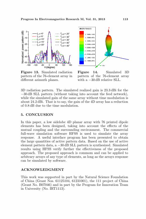
To verify the proposed approach further, the full planar array with76 elements is also simulated with the equivalent excitations. Figure 13shows the simulated far field pattern at the center frequency f0 fromϕ = 0◦ to 45◦. It can be clearly seen that the SLLs in different azimuthplanes are all about−30.0 dB. The front-to-back ratio of the 76-elementplanar array is about 38 dB. The patterns in other azimuth planes havethe same results. For more intuitive view, Figure 14 illustrates the

Progress In Electromagnetics Research M, Vol. 31, 2013 113

-180 -120 -60 0 60 120 180

-40

-30

-20

-10

0 f0, ϕ = 25°

f0, ϕ = 30°

f0, ϕ = 35°

f0, ϕ = 40°

f0, ϕ = 45°

Norm

aliz

ed pow

er pattern

(dB

)

θ (degree)

f0, ϕ =0°

f0, ϕ =5°

f0, ϕ =10°

f0, ϕ =15°

f0, ϕ =20°

-50

Figure 13. Simulated radiationpattern of the 76-element array indifferent azimuth planes.

Figure 14. Simulated 3Dpattern of the 76-element arraywith a −30 dB relative SLL.

3D radiation pattern. The simulated realized gain is 23.3 dBi for the−30 dB SLL pattern (without taking into account the feed network),while the simulated gain of the same array without time modulation isabout 24.2 dBi. That is to say, the gain of the 4D array has a reductionof 0.8 dB due to the time modulation.

5. CONCLUSION

In this paper, a low sidelobe 4D planar array with 76 printed dipoleelements has been designed, taking into account the effects of themutual coupling and the surrounding environment. The commercialfull-wave simulation software HFSS is used to simulate the arrayresponse. A useful interface program has been presented to obtainthe large quantities of active pattern data. Based on the use of activeelement pattern data, a −30 dB SLL pattern is synthesized. Simulatedresults using HFSS verify further the effectiveness of the proposedapproach. The proposed approach is commom and can be applied toarbitrary arrays of any type of elements, as long as the arrays responsecan be simulated by software.

ACKNOWLEDGMENT

This work was supported in part by the Natural Science Foundationof China (Grant Nos. 61125104, 61231001), the 111 project of China(Grant No. B07046) and in part by the Program for Innovation Teamin University (No. IRT1113).

114 Zhu et al.

REFERENCES

1. Shanks, H. E. and R. W. Bickmore, “Four-dimensionalelectromagnetic radiators,” Can. J. Phys., Vol. 37, 263–275,Mar. 1959.

2. Kummer, W. H., A. T. Villeneuve, T. S. Fong, and F. G. Terrio,“Ultra-low sidelobes from time-modulated arrays,” IEEE Trans.Antennas Propag., Vol. 11, 633–639, Nov. 1963.

3. Yang, S., Y. B. Gan, and A. Qing, “Sideband suppression in time-modulated linear arrays by the differential evolution algorithm,”IEEE Antennas Wireless Propag. Lett., Vol. 1, 173–175, Dec. 2002.

4. Yang, S., Y. B. Gan, and P. K. Tan, “Comparative study oflow sidelobe time modulated linear arrays with different timeschemes,” Journal of Electromagnetic Waves and Application,Vol. 18, No. 11, 1443–1458, 2004.

5. Yang, S., Y. Chen, and Z. Nie, “Simulation of time modulatedlinear antenna arrays using the FDTD method,” Progress InElectromagnetics Research, Vol. 98, 175–190, 2009.

6. Pal, S., S. Das, and A. Basak, “Design of time-modulated lineararrays with a multi-objective optimization approach,” Progress InElectromagnetics Research B, Vol. 23, 83–107, 2010.

7. Rocca, P., L. Poli, G. Oliveri, and A. Massa, “A multi-stageapproach for the synthesis of sub-arrayed time modulated lineararrays,” IEEE Trans. Antennas Propag., Vol. 59, 3246–3254, 2011.

8. Zhu, Q., S. Yang, L. Zheng, and Z. Nie, “A patternsynthesis approach in four dimensional antenna arrays withpractical element models,” Journal of Electromagnetic Waves andApplications, Vol. 25, No. 16, 2274–2286, 2011.

9. Chen, Y., S. Yang, and Z. Nie, “Synthesis of satellite footprintpatterns from time-modulated planar arrays with very lowdynamic range ratios,” Int. J. Numer. Model, Vol. 21, 493–506,2008.

10. Poli, L., P. Rocca, L. Manica, and A. Massa, “Timemodulated planar arrays analysis and optimization of the sidebandradiations,” IET Microw. Antennas Propag., Vol. 4, No. 9, 1165–1171, 2010.

11. Rocca, P., L. Poli, G. Oliveri, and A. Massa, “Synthesis of time-modulated planar arrays with controlled harmonic radiations,”Journal of Electromagnetic Waves and Applications, Vol. 24,Nos. 5–6, 827–838, 2010.

12. Li, G., S. Yang, Y. Chen, and Z. Nie, “A novel electronic beamsteering technique in time modulated antenna arrays,” Progress

Progress In Electromagnetics Research M, Vol. 31, 2013 115

In Electromagnetics Research, Vol. 97, 391–405, 2009.13. Poli, L., P. Rocca, G. Oliveri, and A. Massa, “Harmonic

beamforming in time-modulated linear arrays,” IEEE Trans.Antennas Propag., Vol. 59, 2538–2545, 2011.

14. Tennant, A., “Experimental two-element time-modulated direc-tion finding array,” IEEE Trans. Antennas Propag., Vol. 58, No. 3,986–988, Mar. 2010.

15. Hong, T., M. Song, and Y. Liu, “RF directional modulationtechnique using a switched antenna array for communicationand direction-finding applications,” Progress In ElectromagneticsResearch, Vol. 120, 195–213, 2011.

16. Rocca, P., L. Manica, L. Poli, and A. Massa, “Synthesis ofcompromise sum-difference arrays through time-modulation,” IETRadar Sonar Navig., Vol. 3, 630–637, 2009.

17. Rocca, P., L. Poli, L. Manica, and A. Massa, “Synthesis ofmonopulse time-modulated planar arrays with controlled sidebandradiation,” IET Radar Sonar Navig., Vol. 6, 432–442, 2012.

18. Poli, L., P. Rocca, G. Oliveri, and A. Massa, “Adaptive nulling intime-modulated linear arrays with minimum power losses,” IETMicrow. Antennas Propag., Vol. 5, 157–166, 2011.

19. Rocca, P., L. Poli, G. Oliveri, and A. Massa, “Adaptive nullingin time-varying scenarios through time-modulated linear arrays,”IEEE Antennas Wireless Propag. Lett., Vol. 11, 101–104, 2012.

20. Hong, T., M. Song, and Y. Liu, “RF directional modulationtechnique using a switched antenna array for physical layersecure communication applications,” Progress In ElectromagneticsResearch, Vol. 116, 363–379, 2011.

21. Kelley, D. F. and W. L. Stutzman, “Array antenna patternmodeling methods that include mutual coupling effects,” IEEETrans. Antennas Propag., Vol. 41, No. 12, 1625–1632, Dec. 1993.

22. Oliveri, G., L. Manica, and A. Massa, “On the impact of mutualcoupling effects on the PSL performances of ADS thinned arrays,”Progress In Electromagnetics Research B, Vol. 17, 293–308, 2009

23. Darwood, P., P. N. Fletcher, and G. S. Hilton, “Mutual couplingcompensation in small planar array antennas,” IEE Proc. —Microw. Antennas Propag., Vol. 145, No. 1, 1–6, Feb. 1998.

24. Yuan, T., L. Li, M. Leong, J. Li, and N. Yuan, “Efficient analysisand design of finite phased arrays of printed dipoles using fastalgorithm: Some case studies,” Journal of Electromagnetic Wavesand Applications, Vol. 21, No. 6, 737–754, 2007.

25. Pozar, D. M., “The active element pattern,” IEEE Trans.

116 Zhu et al.

Antennas Propag., Vol. 42, No. 8, 1176–1178, Aug. 1994.26. Yang, S. and Z. Nie, “Mutual coupling compensation in

time modulated linear antenna arrays,” IEEE Trans. AntennasPropag., Vol. 53, No. 12, 4182–4185, Dec. 2005.

27. Bernardi, G., M. Felaco, and M. D’Urso, “A simple strategyto tackle mutual coupling and platform effects in surveillancesystems,” Progress In Electromagnetics Research C, Vol. 20, 1–15, 2011.

28. He, Q. and B. Wang, “Design of microstrip array antenna by usingactive element pattern technique combining with Taylor synthesismethod,” Progress In Electromagnetics Research, Vol. 80, 63–76,2008.

29. He, Q., B. Wang, and W. Shao, “Radiation pattern calculationfor arbitrary conformal arrays that include mutual-couplingeffects,” IEEE Antennas Propag. Magazine, Vol. 52, No. 2, 57–63, Apr. 2010.

30. Pozar, D. M., “A relation between the active input impedanceand the active element pattern of a phased array,” IEEE Trans.Antennas Propag., Vol. 51, No. 9, 2486–2489, Sep. 2003.

31. Kelley, D. F., “Relationships between active element patternsand mutual impedance matrices in phased array antennas,” Proc.IEEE Antennas Propag. Symp., 524–527, 2002.

32. Pal, S., B.-Y. Qu, S. Das, and P. N. Suganthan, “Optimalsynthesis of linear antenna arrays with multi-objective differentialevolution,” Progress In Electromagnetics Research B, Vol. 21, 87–111, 2010.

33. Li, R., L. Xu, X.-W. Shi, N. Zhang, and Z.-Q. Lv, “Improveddifferential evolution strategy for antenna array pattern synthesisproblems,” Progress In Electromagnetics Research, Vol. 113, 429–441, 2011.

34. Rocca, P., G. Oliveri, and A. Massa, “Differential evolution asapplied to electromagnetics,” IEEE Antennas Propag. Magazine,Vol. 53, 38–49, 2011.

35. Zhu, X., S. Yang, and Z. Nie, “Full-wave simulation of timemodulated linear antenna arrays in frequency domain,” IEEETrans. Antennas Propag., Vol. 56, No. 5, 1479–1482, 2008.

36. Poli, L., P. Rocca, L. Manica, and A. Massa, “Pattern synthesisin time-modulated linear arrays through pulse shifting,” IETMicrow. Antennas Propag., Vol. 4, No. 9, 1157–1164, 2010.