design of a simplified test track for automated...
TRANSCRIPT

DESIGN OF A SIMPLIFIED TEST TRACK FOR AUTOMATED TRANSIT
NETWORK DEVELOPMENT
A Thesis
Presented to
The Faculty of the Department of Mechanical Engineering
San José State University
In Partial Fulfillment
of the Requirements for the Degree
Master of Science
by
Adam L. Krueger
May 2014

© 2014
Adam L. Krueger
ALL RIGHTS RESERVED

The Designated Thesis Committee Approves the Thesis Titled
DESIGN OF A SIMPLIFIED TEST TRACK FOR AUTOMATED TRANSIT
NETWORK DEVELOPMENT
by
Adam L. Krueger
APPROVED FOR THE DEPARTMENT OF MECHANICAL ENGINEERING
SAN JOSÉ STATE UNIVERSITY
May 2014
Dr. Burford Furman Department of Mechanical Engineering
Dr. Neyram Hemati Department of Mechanical Engineering
Dr. Ping Hsu Department of Electrical Engineering
ABSTRACT
DESIGN OF A SIMPLIFIED TEST TRACK FOR AUTOMATED TRANSIT
NETWORK DEVELOPMENT
by Adam L. Krueger
A scaled test platform has been developed for the purpose of testing, validating,
and demonstrating key concepts of Automated Transit Networks (ATN). The test
platform is relatively low cost, easily expandable, and it will allow future research and
development to be done on control systems for ATN.
The test platform and reference vehicle were designed to adhere to a requirements
document that was constructed to specify the necessary features of a fully functioning
design. The work described in this thesis adheres to the phase one implementation of the
requirements document. The vehicle and track were designed using commercially
available computer aided design software. The prototype track was then assembled, and
the vehicles were manufactured using a finite deposition three-dimensional printer. A
control system was designed to control the velocity and position of the vehicle. This was
accomplished using the feedback of a linear encoder that was designed and laid along the
length of the track.
The vehicle functioned successfully according to the design requirements
document. Testing showed that the vehicle is able to move to a specified position at a
predetermined speed. Additionally, testing showed that a vehicle can maintain a
specified following distance behind another vehicle within twenty millimeters. The
vehicle and track can be used in the future to evaluate and validate specific questions
regarding the implementation of an ATN system.

v
ACKNOWLEDGEMENTS
This thesis is the result of the work of many individuals. I would first like to
thank my committee Chair, Dr. Burford Furman, for his extensive support throughout the
project. I would also like to thank my committee members, Dr. Neyram Hemati and Dr.
Ping Hsu, for their input on this thesis. Jeff Davis from Lea+Elliott also provided a
significant amount of support with the design requirements document, while gently
guiding me in the correct direction, and pointing out roadblocks ahead. Lastly, I would
like to dedicate this thesis to my family and friends for supporting me with in all of my
pursuits.

vi
TABLE OF CONTENTS
Chapter 1 Introduction ........................................................................................................ 1
Objective ....................................................................................................................... 2
Literature Review.......................................................................................................... 4
Introduction ............................................................................................................. 4
Motivations and concerns. ...................................................................................... 5
Features of ATN systems available ........................................................................ 8
Brief history of ATN ............................................................................................. 11
Development work on ATN.................................................................................. 14
ULTra .............................................................................................................. 14
2getthere .......................................................................................................... 15
Vectus ............................................................................................................. 16
MagneMotion .................................................................................................. 18
Taxi 2000 ........................................................................................................ 21
Aerospace Corporation ................................................................................... 23
Conclusions and implications for this study ......................................................... 25
Chapter 2 Methodology .................................................................................................... 27
Chapter 3 Results and Discussion ..................................................................................... 28
Design ......................................................................................................................... 28
Track design. ......................................................................................................... 29
Vehicle design ....................................................................................................... 31
Linear encoder ...................................................................................................... 37

vii
Communication system. ........................................................................................ 41
System Identification .................................................................................................. 42
System Controller ....................................................................................................... 52
Position controller ................................................................................................. 54
Cascaded position velocity controller ................................................................... 57
Multiple Vehicle System............................................................................................. 66
Chapter 4 Conclusions and Recommendations for Future Work ..................................... 69
References. ........................................................................................................................ 72
Appendix A System Design Requirements ....................................................................... 75
Appendix B Bill of Materials of the Track Assembly ...................................................... 81
Appendix C Bill of Materials for the Vehicle Assembly .................................................. 82
Appendix D Drawings of Custom Parts............................................................................ 83
Appendix E Matlab Proportional Controller Code ........................................................... 97
Appendix F Matlab Cascaded Controller Code ................................................................ 98
Appendix G Microcontroller Code for the Vehicle .......................................................... 99

viii
LIST OF FIGURES
Figure 1. Cabintaxi full-scale prototype system .............................................................. 13
Figure 2. ULTra commercial system ............................................................................... 15
Figure 3. 2getthere commercial system ........................................................................... 16
Figure 4. Vectus commercial system. .............................................................................. 17
Figure 5. MagneMotion scale prototype .......................................................................... 19
Figure 6. Taxi 2000’s scale prototype.............................................................................. 22
Figure 7. Aerospace Corporation’s scale prototype ......................................................... 24
Figure 8. Isometric view of track section. ........................................................................ 29
Figure 9. Top view of prototype guideway ...................................................................... 30
Figure 10. Isometric view of prototype guideway ........................................................... 31
Figure 11. Multiple loop track. ........................................................................................ 31
Figure 12. Bottom view of ATN vehicle ......................................................................... 33
Figure 13. Isometric view of ATN vehicle ...................................................................... 34
Figure 14. Isometric view of vehicle and track................................................................ 35
Figure 15. Finite element analysis of flexure ................................................................... 36
Figure 16. Section of linear encoder ................................................................................ 37
Figure 17. Line sensor signal response ............................................................................ 38
Figure 18. Linear encoder spacing ................................................................................... 39
Figure 19. Quadrature encoder signal .............................................................................. 41
Figure 20. Free body diagram of vehicle ......................................................................... 43
Figure 21. Free body diagram of the motor ..................................................................... 44

ix
Figure 22. Electrical diagram of the motor. ..................................................................... 44
Figure 23. Motor characterization of ke ........................................................................... 50
Figure 24. System plant identification ............................................................................. 51
Figure 25. Block diagram of a system with a proportional gain controller ..................... 52
Figure 26. Root locus of the open loop transfer function ................................................ 53
Figure 27. Step response of the vehicle with a proportional gain controller. .................. 54
Figure 28. Block diagram of the system with a PID controller ....................................... 55
Figure 29. Zeigler-Nichols criterion data for position control. ........................................ 56
Figure 30. Position with PID controller. .......................................................................... 57
Figure 31. Velocity with a step voltage input .................................................................. 58
Figure 32. Block diagram of cascaded controller. ........................................................... 59
Figure 33. Zeigler-Nichols criterion data for velocity control. ........................................ 60
Figure 34. Root locus of cascaded controller................................................................... 62
Figure 35. Closed loop pole and zero map of the cascaded controller. ........................... 63
Figure 36. Theoretical step response of the cascaded controller. .................................... 64
Figure 37. Position with cascaded position velocity controller. ...................................... 64
Figure 38. Velocity with cascaded position velocity controller. ..................................... 65
Figure 39. Velocity of two moving vehicles .................................................................... 67
Figure 40. Position with two vehicles with cascaded controller ...................................... 67
Figure 41. Difference in vehicle position ........................................................................ 68

1
Chapter 1 Introduction
Transportation systems in use today are unsustainable. Most people drive
automobiles as their current mode of transportation. There are inherent problems with
using the automobile as a primary means of transportation in urban areas, which include
limited fossil fuels, declining petroleum reserves, rising commute times, and growing
pollution. Cities have tried to provide public transportation systems as alternative forms
of transportation; however, the systems have not been widely adopted due to high costs,
inconvenient schedules and coverage areas, and long commute times. Researchers at San
José State University and in Sweden are working on solar-powered, Automated Transit
Networks (ATN) as a potential solution to the problems with current transportation just
described.
An ATN is a networked system of vehicles that operate autonomously on a
dedicated guideway, which uses offline stations to carry passengers on demand from their
origin to a specified destination. The concept has also been called Personal Rapid
Transit (PRT) or pod cars. The system differs from conventional public transportation
systems, such as light and heavy rail, because vehicles pick passengers up when they are
requested, similar to a taxi, rather than on a set schedule as with conventional transit.
On-demand travel allows the system to adapt to the passenger rather than the passenger
adapting to the system. Additionally, the system transports passengers from their origin
to their destination with no intermediate stops. An ATN is able to achieve this due to off-
line stations which allow mainline traffic to continue unimpeded. Additionally, vehicles
in an ATN are designed to hold individuals or small groups of passengers who may wish

2
to travel together rather than with strangers. This is not only an attractive way to travel
for passengers, but it also allows for smaller, lighter vehicles that potentially could be
powered electrically through solar photovoltaic panels mounted to the guideways and at
stations. A system configured in this way would have the potential to capture enough
energy to power the network within its footprint in an urban setting. Finally, most
experts in the ATN field agree that the system should have a dedicated, elevated
guideway used only for ATN vehicles. An elevated guideway provides several important
benefits.
Machines and humans are separated, which results in improved safety.
Construction is less expensive compared to tunneling underground.
Guideways can be placed in existing rights-of-way, such as roadways, to
reach populated areas that have already been developed.
Objective
This thesis achieved the following objectives. First, simplified vehicles made of
relatively inexpensive components were developed. In parallel, a test track was
developed, which the vehicles travel on. The test track has four offline stations to
demonstrate vehicle switching on diverging sections of track. These offline stations
simulate passenger loading zones.
The system developed will continue to be used as an early stage prototype that
can be used to test, validate, and demonstrate concepts used in ATN. As an example, the
system can be used to validate various passenger loading scenarios, the effect of headway

3
on capacity, and passenger wait time. The results of these studies will allow ATN to be
better understood and will advance the state-of-the-art of ATN as a whole.
Important features of the system designed were that it was low cost, portable, easy
to expand, and easy to assemble. It was necessary for the system to be low cost so that an
expanded network could be built with modest funding. In this way, the network aspect of
ATN with multiple vehicles and multiple stations could be investigated. An expanded
network of guideways will enable investigation of system capacity, vehicle routing,
empty vehicle management, and passenger surge loading before having to invest in a
city-wide full-scale implementation.
The system should be portable so that it can be demonstrated to the public at
places such as a city government center or library. This will facilitate educating the
public about ATN and its benefits by showing how a model ATN system will look and
how it will function.
The outcomes of the objectives described advance the state of the ATN by
providing a platform where specific ATN concepts can be constructed, tested, and
demonstrated. Currently, there are few small scale systems where ATN systems can be
tested. There are many simulations of ATN systems, but there is little experimental data
available. Additionally, most prototype systems are not small or accessible enough to be
demonstrated to the public. The system described herein allowed experimental data to be
collected and also allowed an ATN system to be demonstrated.

4
Literature Review
Introduction. The idea for Automated Transit Networks has been around since
at least 1953 (McDonald, 2013). Since then, many ATN systems have been conceived
and designed including Cabintaxi, Vectus, Beamways, Ultra, H-bahn, and Skytran
(McDonald, 2013). Of the many that have been designed, there are only a few that have
been built and are functioning, which are Vectus, 2getthere, and ULTra. There are many
reasons that ATN systems have taken this long to develop. This thesis will describe the
state of development of ATN by first explaining the motivations and concerns related to
ATN, detailing the important features of an ATN system, and providing the history of
ATN. This background will give insight into the currently available ATN systems.
Next, the currently available scale prototype ATN systems will be discussed.
Large scale commercial systems have still yet to be implemented even though ATN has
come a long way with fully functioning systems. This is largely due to skepticism about
the cost, return on investment, and functionality of a large capacity ATN system
(Aerospace Corporation, 2012). Skepticism continues, even though there has been a
substantial amount of theoretical and empirical work that demonstrates the functionality
of ATN systems, as well as computer simulations that show the effectiveness of ATN
systems. One way to overcome the skepticism is to install more ATN systems in order to
validate the claims of ATN proponents. The advantage of model systems is that they
demonstrate the effectiveness of an operational system without the need for as many
simplifications needed for theoretical of simulation analyses. Prototype and model

5
systems that have been developed will be described in detail so that future models can
benefit from the triumphs and challenges of past work.
Motivations and concerns. ATN systems are often controversial and have
become a topic of debate. A great deal of research has been conducted on the feasibility
of the ATN systems, most of which has theoretically proven both the efficacy of the
systems and its positive impact at alleviating congestion in highly populated areas. This
research has recently led to the startup of many companies designing ATN systems and
cities conducting studies on the feasibility of ATN systems including New Jersey
(Carnegie & Voorhees, 2007), Fresno, CA (Kimberly Horn and Associates, Inc., 2010),
and San José, CA (Aerospace Corporation, 2012). Still, critics of ATN systems claim
that ATN systems are unproven, costly, and too risky. Even the studies that have been
performed for specific cities suggest that more research needs to be done of the topic
before cities are willing to invest any money. As an example, San José paid for a
feasibility study by Aerospace Corporation with the objective of performing a “rigorous,
comprehensive analysis of the technology before determining whether to consider
building a system” (Aerospace Corporation, 2012, p. 3). The results of the study stated
that building an ATN system at the current time, in 2012, would be risky for the city
because of the number of unanswered questions such as network capacity, power
requirements, regulatory issues, and estimated cost. Similar results were found in studies
performed in New Jersey stating that “PRT technology has not yet advanced to a state of
commercial readiness” (Carnegie & Voorhees, 2007, p. 5). As a direct result of these
claims, more research and development is needed to address the unanswered questions.

6
Specifically, research needs to be performed in the areas that these studies deem
inadequate to reduce the risk associated with ATN systems.
If ATN can overcome the obstacles that are outlined in these studies, it has the
potential to revolutionize transportation much in the same way the automobile did. John
Anderson (2000), an expert in the field of ATN, provided a comprehensive list of the
benefits of an ATN system in his review of ATN systems. Austin (2001) also described
how ATN has the potential to revolutionize transportation in her description of idealistic
transportation. A subset of the benefits is listed here.
Fast, safe, private, secure, and all-weather transportation
Reduction of roadway congestion
Reduction accidents while travelling
Reduction of air and noise pollution
Reduction of energy usage
Low street repair costs
Improved mobility
In order for ATN to become a largely commercially based system, some
skepticism with ATN systems needs to be overcome. The previous section alluded to
some of the concerns with ATN. The concerns that were discovered by cities looking to
implement ATN will be described below because these organizations are the ones that are
looking seriously into building an ATN system.
Average travel speed and overall trip times. Although there are many
studies and simulations that have tried to describe the overall trip times,

7
there are still questions about how this will work in practice. The major
concern is that all of the studies that have been performed are conceptual
(Carnegie & Voorhees, 2007).
System and station capacity. Capacity of stations and the total system
continues to be a concern, even though theoretical capacities of 10,000
people per hour per direction can be achieved (Carnegie & Voorhees,
2007). The main concern is how the system will respond in times of peak
usage. Large wait times would minimize the effectiveness of the systems
(Aerospace Corporation, 2012).
Capital costs. The overall cost of the system is always a concern,
especially when there is a large upfront cost that needs to be assumed by
the public. There are preliminary estimates that predict ATN could cost
approximately $25 million per mile of guideway (Carnegie & Voorhees,
2007).
Operating and maintenance costs. There is a sizable risk in operating
and maintenance costs required for an ATN system largely because these
costs are contingent on a specific ATN design (Carnegie & Voorhees,
2007). Additionally, costs associated with system outages are difficult to
define.
Energy use and environmental impact. The energy use of the system is
contingent on the size of the system that will be implemented. This is
largely affected by vehicle and guideway design that each individual

8
system will use. Aerospace Corporation (2012) found that heating and
ventilation concerns will be a large part of the power consumed.
Each of these concerns will need to be addressed in more detail for ATN to be
more widely accepted. However, it seems that the major concerns with ATN are not that
the system will not conceptually work. There are many papers that prove otherwise. The
major concern is that there are few fully operational ATN systems available and the
success of an ATN system is highly contingent on its final design. Therefore, many cities
are hesitant to invest a large amount of capital with little knowledge of the final designs.
More prototype systems, both small and full-scale, are needed in order to gain confidence
in the concept of ATN as a whole.
Features of ATN systems available. The design of an ATN system is of the
utmost concern when determining its effectiveness in a desired location. As a result,
there are many important features that need to be incorporated into an ATN system for it
to operate effectively and efficiently. These include capacity, switching, suspended
versus supported vehicles, vehicle design, guideway design, reliability, safety, and energy
considerations (Anderson, 2000).
Capacity is the single most important characteristic of ATN systems aside from
safety for an effective ATN system. Capacity of the system directly affects the number
of people the system can handle, wait times for passengers, and in turn, acceptance of the
system. Capacity also has a large impact on the entire cost of the system. Larger
vehicles can handle more passengers, which increases capacity; however, larger vehicles
also require larger guideways to support the larger weight. Anderson (2005) describes

9
how a system of many small vehicles versus a system with fewer larger vehicles with
equivalent capacity will have a guideway weight and cost reduced by a factor of at least
20. Construction of guideways is the most expensive part of an ATN system (Anderson,
2000). Therefore, it is worth considering the possibility of using smaller vehicles.
Smaller vehicles cannot carry as many people, so inherently the number of vehicles in
operation would need to be greater. As a result, capacity and vehicle sizing are not
trivial problems. Anderson (1984) has provided a detailed analysis of the capacity, cost,
and size of traditional train systems versus an ATN system. He finds that it is cost
effective to construct a properly designed ATN over a traditional bus transportation
system. Still, the carrying capacity of each vehicle as well as the carry capacity of the
system needs to be carefully considered for a system to be an effective transport method.
Vehicle design is the second most important consideration of an ATN system.
The vehicle design will dictate the capacity, the cost of the vehicle, as well as the cost of
a guideway for it to run on. Furthermore, it has a large effect on the safety of the system
and passenger comfort/acceptance. The ideal vehicle for a system will be relatively low
capacity, low weight, and low cost. Approximately 90% of vehicles on the road during
peak hours contain 1.2 persons (Anderson, 2000). Therefore, an ideal ATN vehicle
would carry roughly the same amount of people. Additionally, research showed that the
operation and maintenance costs are reduced if the smallest vehicles are used. As a
result, special consideration should be given to the vehicle design to minimize size,
weight, and cost.

10
A switching mechanism is needed on the vehicle so that the vehicle can travel on
a guideway that splits. Track splits are necessary so a vehicle can diverge off the
guideway into a station or so that tracks that service different areas. The mechanism for
which switching occurs has a great impact on the safety, reliability, and the capacity of
the system. The switching mechanism that is used should be safe and repeatable. One of
the considerations for a safe system is to have a locking system to ensure that the system
cannot impale itself on a diverging section of track.
Combustion of hydrocarbon fuels is an increasing concern as global warming
increases. For this reason, ATN should strive to minimize use of fossil fuels. Although
the energy that is required for an ATN system is based on many factors, including vehicle
design, propulsion system, guideway design and passenger loading, steps can be taken to
minimize the energy consumption used in any system. The control system will have a
large impact on the overall consumption of energy. For example, minimizing
intermediate stops will greatly increase the overall efficiency of the system (Anderson,
2000). Regenerative braking can capture some of the energy normally lost during
intermediate stops, but this is just a percentage of the energy needed to accelerate to
operating speed. Additionally, the maximum acceleration needed in each vehicle will
dictate the amount of energy the system consumes. “The maximum power
requirement…can be cut almost in half with little penalty by gradually reducing
acceleration above about half line speed” (Anderson, 2000, p. 15). As a result, special
attention should be taken to evaluate the control systems that dictate intermediate stops,
deceleration, and overall acceleration to minimize the energy usage of the system.

11
Brief history of ATN. Numerous papers have been written examining the history
of ATN, so that information from the past can be used to aid future development.
McDonald’s review gave a comprehensive review of ATN, including its origins.
McDonald (2013) stated that the idea of ATN was conceived in 1953 independently by
Donn Fichter and Ed Haltom. This information was supported by Anderson (2000) in
his independent review of ATN. However, even though the idea of ATN was discovered
in the early 1950s, research on the topic was largely un-collaborative until the US
government endorsed the idea by passing the Urban Mass Transportation Act in 1964
(United States, 1964). Once the act was passed, there were many funded programs that
sprung up leading to many research papers and company startups including Aerospace
Corporation. Also, as a direct result of the federal funding surrounding ATN, the
Morgantown ATN system was built (McDonald, 2013).
The Morgantown ATN system was funded and built because West Virginia
University had limited space for the campus to grow while an increased number of
students wanted to attend in the late 1960s. The solution was to build a separate campus
1.5 miles away. This split an already-separated campus into three campus locations.
Congestion in the city quickly became a problem because of the increase traffic between
campus locations. During this time, ATN was being worked on extensively, and it was
considered as a concept to mollify the congestion problems. University officials
proposed running a feasibility study on the concept of ATN in Morgantown. The
feasibility study was conducted in 1970, which led to a federal grant for the construction
of the system (Sproule & Neumann, 1991). The system became operational carrying

12
passengers on October 3, 1975. This system was plagued with problems during the initial
months of operation including vehicle malfunctions, sticking turnstiles, weather related
problems, and exceeding the budget by a factor of four. Despite its initial setbacks, the
system is still running today with an “operating reliability of over 99%” (Sproule &
Neumann, 1991, p. 276).
The Aerospace Corporation (2014) had a large hand in getting the technology to a
point that the Morgantown system could be built. It was set up after the Urban Mass
Transportation Act of 1964 was passed as a non-profit entity and was funded by the
government to develop technology of public importance. Jack Irving (1978) led the
efforts of the company in developing the concept of an ATN system. They spent a large
amount of time performing paper studies along with experimental design. The
culminating project of the company was to develop a functioning prototype ATN system.
After the company developed this, they published a book called Fundamentals of
Personal Rapid Transit where they disclosed the lion share of work that the company had
done with regard to ATN to spur public interest and share their knowledge with potential
companies who would take the concept to a commercial state (Irving, 1978).
The surge of funding in ATN in the United States also spurred interest in other
countries including Great Britain, Japan, Germany, France, Sweden, and Canada. Many
companies spun out of the research performed in these countries with some large scale
prototypes being constructed in countries such as Japan (McDonald, 2013).
The Cabintaxi program sprung out of international funding in Germany in 1969.
The original development of the Cabintaxi system was started by two separate firms

13
Messerschmitt-Bolkow-Blohm (MBB) and Demag. Then, in 1972, the German
government facilitated combining the companies and funding the ATN project. The
Cabintaxi system was developed as a result. The Cabintaxi system consisted of a two-
way elevated track where one direction of the traffic moved above the guideway while
the other traveled below the guideway. A full-scale test track was operational in 1976
with 24 vehicles and a 1.1 mile test track (Carnegie & Voorhees, 2007). A picture of this
is shown in Figure 1.
Figure 1. Cabintaxi full-scale prototype system (Carnegie & Voorhees, 2007). Two-way
traffic is achieved by having one traffic direction above the guideway and the opposite
direction traffic below the guideway. Reprinted with permission from Cabintaxi.
Extensive testing was performed on this track, and it was studied expansively by
outside firms interested in ATN, including many United States companies. There was a
plan for a large scale system to be built in Hamburg, Germany, but lack of government
funding led to the end of the program in 1980. A United States firm absorbed the
technology, but the company is currently looking for funding to perform additional
research and implement the technology at a commercial site.

14
Over the next 50 years there have been many attempts at constructing a working
ATN system. Today, there are several working ATN systems, although none of them are
yet working under ideal conditions to realize the full benefits of ATN. The original
concepts of ATN were ambitious and before their time. The technology needed to
implement ATN was not available in the 1970s, making it expensive and difficult to
design and construct a working system (Lowson, 2011). Still, the potential benefits of
ATN have kept interest high in the technology. This can be seen in the large amount of
funding for research that has cropped up over the years.
Development work on ATN. Research continues today on the concepts of ATN
by both academia and private industries. There are many companies that have
developed ATN systems that are waiting for potential sites to adopt them. These
companies include MagneMotion Maglev, Vectus, Beamways, Ultra, H-bahn, 2getthere,
and Skytran. ULTra, 2getthere, and Vectus have developed commercial systems and
have implemented or are implementing them at specific sites.
ULTra. The ULTra system is operational in London, United Kingdom at the
Heathrow airport. It began operation in 2010 with 2.4 miles of guideway, three stations,
and 21 vehicles. The vehicles operate at a four second headway. This gives a one way
capacity of 3600 seats per hour (Lowson, 2011). The guideway costs $15 million/mile of
one-way guideway (Helmer, 2009). This is less than the cost of developing a footbridge
for walking pedestrians. The weight loading factor needed for pedestrians is 5000 N/m2
whereas the loading factor needed for the ULTra systems is 2000 N/m2 (Lowson, 2011).
The system’s vehicles are not track guided, but instead have a steering mechanism and

15
four rubber tires. The system steers itself by using dead reckoning and sensors that relay
to the control system the distance from the walls on the vehicle sides. The vehicle design
is shown in Figure 2.
Figure 2. ULTra commercial system (Lowson, 2011). The system operates on an
exclusive roadway with no rails. Reprinted with permission from ULTra.
2getthere. The 2getthere system is located in Masdar City, Abu Dhabi. It began
operation in 2012 with 1.1 miles of guideway, five stations, and thirteen vehicles
(2getthere, 2012). The current system is the link for the Masdar Institute of Science and
Technology (MIST) (Muller, 2010). This is part of an initiative to make Masdar City the
most sustainable city in the world. The city plans to not use any fossil fuel powered
vehicles in the city. The plan is to eventually grow the ATN system to 3000 vehicles and
85 stations (2getthere, 2012). An example of a typical loading station is shown in Figure
3.

16
Figure 3. 2getthere commercial system (2getthere, 2012). Vehicle stations are shown
where passengers can embark and disembark the vehicle. Reprinted with permission
from 2getthere.
Vectus. Vectus is currently implementing a system in Suncheon Bay, South
Korea. This system was expected to open in 2013 with 6 miles of guideway and 40
vehicles (Pemberton, 2013), but it is still undergoing system testing. The guideway is
double tracked allowing two-way travel of vehicles along the guideway. A picture of the
system is shown in Figure 4.

17
Figure 4. Vectus commercial system. The picture shows the double-tracked Vectus
system in Suncheon Bay, South Korea. (Vectus Ltd., 2012). Reprinted with permission
from Vectus.
The guideway being built has large pilings buried approximately 30 meters into
the terrain due to the earthquake activity in the region. The system will start operation
with two stations with the possibility of expansion. It is expected that the system will
have 5000 passengers per day (Muller, 2010). The guideway is comprised of simple steel
tubing. The mechanical switching mechanism is mounted in the vehicle, and is comprised
of a wheel that moves to the outside of the diverging track, which guides the vehicle
along the correct track (Muller, 2010).
The current systems that are available have limitations because they cannot scale
to the capacity levels that the original promoters of ATN anticipated. Additionally,
research is needed to prove that the capacities envisioned can be achieved. As a result,
there is a need for robust scale models to further develop the technology.

18
Prototype systems provide many benefits to learning about ATN systems.
Simulations can provide intuitive information about how the systems will react. There
are many simulations that are currently available that show how the control systems will
work; however, simulations rarely provide a complete picture of the system. Instead,
simulations use assumptions to simplify the system to make it easier to model.
Assumptions still need to be made when assembling a prototype, but even a scale
prototype will encounter similar disturbances that will be encountered in a full-scale
system. As a result, a realistic system can be developed and tested for minimal costs
compared to a full-scale system.
Many ATN developers have realized the benefits of developing prototype
systems. The systems vary in size and scale. Companies such as MagneMotion, Vectus,
Beamways, Ultra, Cabintaxi, Cabinlift, and Skytran have all built full size prototypes of
their systems. There are also some ATN developers that realized the benefits of
developing a scale system including MagneMotion, Taxi 2000, and Aerospace Corp. As
described above, these small-scale systems are used to show operational systems, while
not making unrealistic assumptions, for a fraction of the cost of a full-scale system or
large-scale prototype. For this reason, the following section will describe each scale
prototype system in detail, describe its advantages, and describe its disadvantages.
MagneMotion. MagneMotion developed a small test track system to showcase
the development of their ATN concepts (Magnovate Technologies, 2013). The test track
was mainly built to feature the effectiveness of their magnetic levitation system. The
system used a Stabilized Permanent Magnet (SPM) suspension to levitate the

19
MagneMotion vehicle. An additional highlight of the system is the track switching
mechanism that MagneMotion uses. MagneMotion claims that this system is passive
because there aren’t mechanical or electrical components (Magnovate Technologies,
2013). In their prototype, the track switching is accomplished by manipulating the track
stabilization fields at the diverging section of track. The field is manipulated to force the
vehicle in the desired direction (Magnovate Technologies, 2013). The merging of the
vehicle onto two converging tracks is handled automatically.
The system has one vehicle that moves on a test track with two switches via a
linear synchronous motor (LSM). The system is shown in Figure 5.
Figure 5. MagneMotion scale prototype. The system has a magnetic levitation ATN
system with one vehicle (Magnovate Technologies, 2013). Reprinted with permission
from Magnovate.
The vehicle shown has onboard radio control. It was designed to handle 20 to 40
passengers. MagneMotion expects that the vehicles could operate in platoons as well as
individually.

20
One of the main advantages of this system is that it effectively demonstrates the
technology used behind both its drive mechanism and switching mechanism from track to
track. A simulation would not intuitively explain the working mechanisms behind these
systems. Furthermore, the system gives an effective representation of how the system
will look because both the vehicle and the track were designed to look realistic from the
outside. This is an important attribute because it shows the aesthetics of the system.
Potential customers can easily get a feel for the aesthetic appeal of the system.
Although this prototype system is effective at showing the effectiveness of the
magnetic levitation system, it lacks the capability to show how the system would react in
many of the operating scenarios including multiple vehicle headways, fast track
switching, multiple vehicle merges, and station overload.
One of the main attributes that people research in ATN is safe vehicle headway.
Vehicle headway is a measurement of distance between two vehicles travelling at a
velocity. Headway is measured by using the time it takes a trailing vehicle to be in the
same position as the leading vehicle. A one vehicle system does not have the ability to
show safe following distances can be achieved. If there were at least a two vehicle
system, safe following distance could be experimentally measured. Additionally, tests
could be conducted to determine how fast a vehicle could stop in an emergency.
Vehicles on ATN systems need to have a fast switching mechanism to quickly
merge or diverge from tracks. For example, if vehicles were following in close proximity
with a low headway, the system should be able to react fast enough so that vehicles do
not miss diverging to a station or another guideway segment. The MagneMotion system
21
does not have the ability to show the speed at which the track can switch to divert
vehicles down multiple paths in real time. In theory, track switching such as this could
be operated almost instantaneously; therefore, the system should not have any problem
switching (Magnovate Technologies, 2013). However, it would be beneficial if this
system had multiple vehicles so that it can show this.
Another main concern with regard to ATN is the ability to make safe merges on
converging tracks. The MagneMotion system does not have the ability to show how
multiple vehicle merges are performed. As a result, it cannot show how the control
system will resolve potential merge conflicts when multiple vehicles want to merge at the
same time. This could be improved by upgrading the prototype to have multiple vehicles.
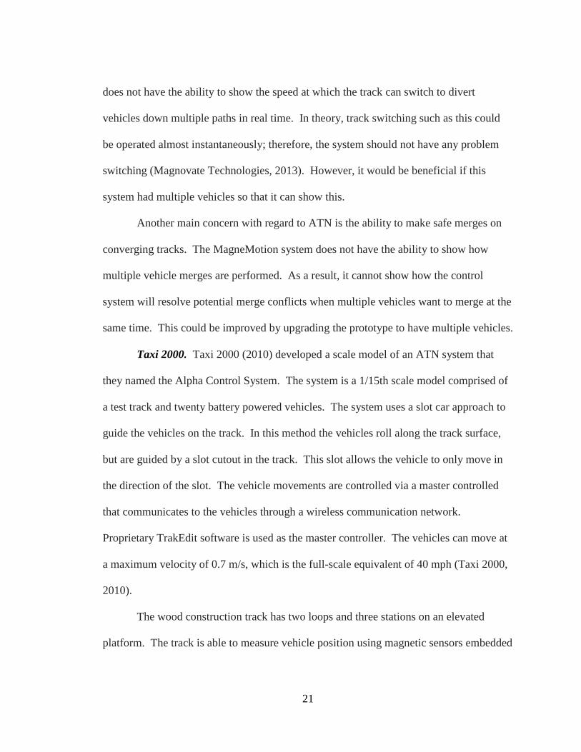
Taxi 2000. Taxi 2000 (2010) developed a scale model of an ATN system that
they named the Alpha Control System. The system is a 1/15th scale model comprised of
a test track and twenty battery powered vehicles. The system uses a slot car approach to
guide the vehicles on the track. In this method the vehicles roll along the track surface,
but are guided by a slot cutout in the track. This slot allows the vehicle to only move in
the direction of the slot. The vehicle movements are controlled via a master controlled
that communicates to the vehicles through a wireless communication network.
Proprietary TrakEdit software is used as the master controller. The vehicles can move at
a maximum velocity of 0.7 m/s, which is the full-scale equivalent of 40 mph (Taxi 2000,
2010).
The wood construction track has two loops and three stations on an elevated
platform. The track is able to measure vehicle position using magnetic sensors embedded
22
in the track to determine the absolute position of the vehicle. A picture of the system is
shown in Figure 6.
Figure 6. Taxi 2000’s scale prototype. The company calls the prototype the Alpha
Control System. It is a 1/15th scale personal rapid transit system (Taxi 2000, 2013).
Reprinted with permission from Taxi 2000.
Some of the advantages of the system are that it can demonstrate multiple vehicle
control with a specific headway, merging and diverging operations, and demonstrate
system loading levels. These are all possible because the system has multiple vehicles
and it has multiple stations for the vehicles to merge and diverge. In fact, this system was
built to specifically test and validate some of the software schemes in the TrakEdit
software (Taxi 2000, 2010). Validating the software was only possible by using multiple
vehicles to demonstrate the various control schemas.

23
The Alpha Control System had a few disadvantages, including lack of passenger
information, lack of a realistic guide way, and overall cost. The system does not have the
ability to display passenger information at the stations. Since passenger movement is at
the heart of ATN, it would be beneficial to show the movement of passenger from
stations to vehicles, and then to destination stations. Passenger indicators would make it
easier to visualize the movement of passengers. Additionally, the system could be used
to demonstrate the movement of empty vehicles to fill current demand at stations as well
as movement of vehicles to fulfill predicted future demand.
Second, the system is costly. The system is extensive, with twenty vehicles, and
each of these vehicles costs money. Additionally, the track is costly to assemble because
there is a significant amount of time invested in cutting the track pieces and assembling
them.
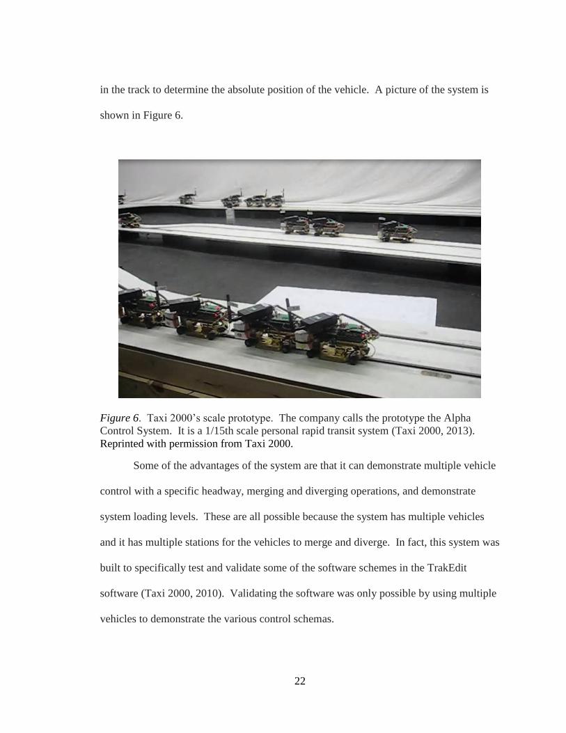
Aerospace Corporation. The Aerospace system was designed and built in 1971.
It was one of the first scale models built to show the concept of ATN. The concept was a
1/10th
scale model consisting of a 45 x 14 foot oval track and three vehicles (Irving,
1978). The vehicles operated using linear electric motors that were onboard each of the
vehicles. The nominal vehicle velocity was 3 ft/s which corresponded to a full-scale
velocity of 20.5 mph. All the propulsion systems in the model were scaled directly to
1/10th
tenth the size of a full-scale system. Also, the dimensions of the motors and track
and the motor power were scaled exactly to 1/10th
of a full-scale system. The mass of the
system was scaled appropriately to account for the inertia of the system when
24
accelerating. In this way, the propulsion system was designed so that it would mimic a
full size model accurately. A picture of the prototype system is shown in Figure 7.
Figure 7. Aerospace Corporation’s scale prototype (Irving, 1978). This is a 1/10th
scale
prototype with three vehicles. Reprinted with permission from Aerospace Corporation.
The main advantage of this system was the effort that was put into sizing the
system appropriately in all facets including size, weight, and propulsion. This accurate
sizing of the system allowed each subsystem to be tested effectively without making
large assumptions. Additionally, the vehicles were designed to look similar to a final
concept. As described above, this showcases the aesthetic appearance of the vehicles.
The outdoor nature of this system also allowed it to be tested against the elements
in a similar situation to how a commercial system would have to perform. Again, this
allowed for thorough testing to be conducted on the prototype in many different types of
conditions.

25
One of the main disadvantages of this system is its size. The 1/10th
scale model
would require ample installation space as well as a large amount of money to fully
implement. Interestingly, Aerospace Corp. selected the scale based on the technology
that was available at the time. Aerospace Corp. did not think that they could effectively
house all the electronics in the vehicles at a smaller scale. Electronics have decreased
orders of magnitude in size since the 1970s. Therefore, a smaller scale would not be a
problem for scale models built today.
Another disadvantage of the system is that it only has one station on the guideway
and only three vehicles. A multiple station prototype has the ability to show how the
vehicles could be used to transport passengers throughout the system without excessive
delays. Demonstration on the movement of empty vehicles is also necessary to show
how the vehicle will respond to unbalanced demand. This would be difficult to do with
only three vehicles and one station.
Conclusions and statement of problem. ATNs have many benefits that can be
realized with a properly developed system. Urban traffic congestion, dependence on
fossil fuel, and reduced emissions are a few of the direct benefits that can be realized
from ATN in addition to many of the indirect benefits that can provide value to a city.
With all these benefits, only a few cities have adopted ATN systems and most of them
have happened only recently. Feasibility studies have shown that most cities have not
adopted ATN systems because they will be assuming too much risk. The studies claim
that the technology is still too immature to risk the capital necessary to implement them.
The current system implementations will help other cities adopt ATN systems as they

26
observe the effectiveness of the ATN implementations. In addition, more research needs
to be performed on key areas of ATN to minimize the risk that interested cities will have
to assume.
Theoretical research as well as conceptual research needs to be performed.
Unfortunately, there are few good physical models of systems that have been
implemented. Implementation of a physical model is important because it can
demonstrate the important features of ATN with a low up front cost. It also provides an
avenue for interested parties to experiment and develop ATN technology further. With
an effective model, many of the benefits of ATN can be discovered, and many of the
problems will be exposed, allowing the world to come closer to an environmentally
responsible, economical solution to transportation that passengers will appreciate.
Even though there are a limited number of scale models, the few shown here offer
insight into the important elements of a scale model. The scale vehicle needs to be small,
easy to manufacture, and minimal cost. These attributes are essential because a scale
system needs to have at least three vehicles to accurately model an ATN system. A
system with fewer vehicles makes it difficult to simulate ATN systems. The Taxi 2000
model shows the benefits of having a complex system.
Additionally, the track needs to be minimal cost, easy to manufacture, and easy to
assemble in custom configurations. An important feature of a scale ATN track is that it
can be configured similar to a full-scale system. As a result, it is important that the track
can be easily constructed to mimic full-scale implementations. Also, the ability to
quickly expand the track and vehicle system will allow more complex systems to be

27
tested. Therefore, special care needs to be taken to quickly and easily expand the track
and size of the vehicle fleet.
Chapter 2 Methodology
Prototype systems are necessary to show the development of the design concept.
There are many steps in the design process that are listed below.
1. Concept
2. Design requirements and design specifications
3. Scale model (functional)
4. Full-scale mock-up (non-functional)
5. Full-scale engineering development prototype
6. Final design
There are few ATN prototype systems that are currently available in the
functional scale model step. One of the reasons for this is that there has been funding
available for the development of full-scale prototype systems in the past. However, scale
models are more effective at building confidence to get additional funding when working
with a limited budget (Transport Innovators, 2013). Still, experts studying ATN have
noted that there is a lack of acceptable scale ATN models. Therefore, a low cost system
that can be used to successfully test, validate, and demonstrate various ATN control
concepts was developed.
In order to design a system that meets all the requirements needed for an effective
ATN model, a design requirements document was developed and it is attached to the end
28
of this document in Appendix A. This document outlines the necessary requirements for
the system to work properly. These requirements were necessary because they helped to
determine what features were needed in the design. This guided the design to ensure the
final system functioned as it was intended. Once this document was complete the design
of the system commenced.
One of the requirements of the system was for it to be track guided and not
independently steered. The reason for this was that it was important for the system to be
similar to a track guided system that has track switching control. As one might expect,
track switching controls could not be developed without a track guided system.
Another requirement was to design a system that approximates a currently
available system. This allows testing and validation of controls schemes on a model
level. The system design was chosen to approximate the Vectus system and other real
systems. Therefore, required features of the design were that the vehicle is supported
underneath, it has guide wheels along the track, and it has a mechanically operated
switching mechanism to guide the vehicle along a diverging section of track.
Chapter 3 Results and Discussion
Design
In the following section, the design of the prototype ATN system is described in
detail. Additionally, a supplementary video of the system was made so that the dynamics
of the system could be better understood. This video was then posted to the internet and
can be viewed by referring to the web site titled “Automated Transit Network (ATN)

29
prototype” posted in the references of this document (Krueger, 2014). Also, drawings of
the custom parts are included in Appendix D for reference.
Track design. Many ideas were developed in the process of designing an
economical, easy to assemble track. The most economical system was constructed of
bent sheet metal strips mounted to a plywood board with screws. This design is shown in
Figure 8.
(a) (b)
Figure 8. Isometric view of track section. The sheet metal part shown forms a vertical
section of track that the vehicle can ride along. The 16 in long part is bolted to plywood
with two tabs that have a hole punched in them.
The overall cost of the track is shown in the bill of materials for the track in
Appendix B. The track guideway has four stations designed to fit in an 8 x 8 foot area.
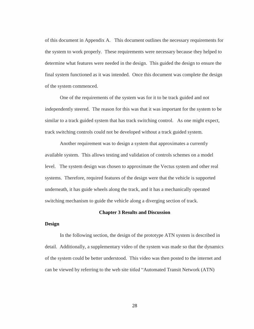
The station locations are shown in Figure 9.
30
Figure 9. Top view of prototype guideway. The guideway is mounted on two plywood
sheets with four stations with one at each of the four corners.
Four stations were incorporated into the track to allow each vehicle to have three
alternate stations where it could travel. A four station system is sufficiently complex so
that the routing algorithms used by each car are not trivial. The final guideway is shown
in Figure 10.
Stations Stations

31
(a) (b)
Figure 10. Isometric view of prototype guideway. The guideway consists of vertical
sheet metal strips that are mounted to plywood by bent tabs.
The track system can be expanded quickly and inexpensively by creating a
diverging section of track that moves to a new area. One example of this is shown in
Figure 11, where an addition loop is added to the existing track.
Figure 11. Multiple loop track. The picture shows an alternate setup of the track where
an additional diverging section of track can be added to expand the track system.
Vehicle design. The vehicle was designed to be able to traverse the guideway
smoothly while having adequate sensors incorporated to control the vehicles.
32
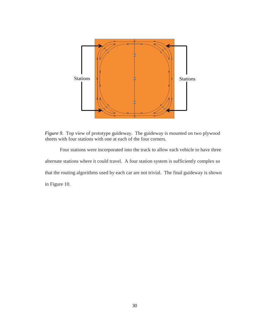
Additionally, the chassis was designed to be inexpensive to minimize costs if the system
is expanded. In order to minimize cost, the chassis was designed around 1/32 scale slot
car parts because these parts are readily available and inexpensive. In order to quickly
fabricate the vehicle, a Stratasys uPrint SE Finite Deposition Model three-dimensional
printer was used. The material used was white acrylonitrile butadiene styrene (ABS)
plastic. The overall size of the vehicle is 94 x 140 x 50 mm and the overall cost of the
vehicle is approximately $157 and the cost breakdown is shown in Appendix C.
The vehicle is powered by three 3.7 volt lithium ion batteries. These batteries are
connected in series to provide power at 11.1 volts to both an Arduino Uno R3
microcontroller and an SN754410 half H-bridge driver. The system is propelled by a
Scalextric C8146 12 V direct current (DC) motor. The drive motor is connected to the
rear axle by a 3:1 gear ratio. This is shown in Figure 12.

33
(a) (b)
Figure 12. Bottom view of ATN vehicle. The drive mechanism of the vehicle is
mounted to the bottom of the vehicle. Wheels mounted on flexures provide vehicle
guidance within the track. Hard stops are behind each flexure to limit their deflection.
The sensors to control the vehicle are three QRE1113 infrared reflectance line
sensors mounted on the bottom of the vehicle (Fairchield Semiconductor, 2009). The
location of the sensors is shown in Figure 12. The line sensors count lines on a linear
encoder mounted on the track. It does this by using the fact that a white surface has a
different reflectivity from a black surface. To take advantage of this principle, the line
sensor shines an infrared beam down and it reflects back onto a detector. The detector
output is a different voltage based on the reflectivity of the material below it. This can be
used to count lines on a linear encoder which allows the position of the vehicle to be
known.
Error
Correction
Sensor
Linear Encoder
Sensors
Flexures
Drive
Motor
Hard Stops

34
The switching mechanism is operated by one 12 V DC motor from a Scalextric
slot car kit. This motor drives a worm gear mechanism which then drives the switching
mechanism up and down. Figure 13 (a) shows the switching mechanism in one position
and Figure 13 (b) shows the switching mechanism in the other position. The worm gear
was chosen to be self-locking so that the switch will stay in position even if a high force
is imposed upon the switch from the track.
(a) (b)
Figure 13. Isometric view of ATN vehicle. The vehicle switching mechanism is
operated by the motor and worm gear mounted to the top of the vehicle. The batteries are
directly behind the motor and the microcontroller is beside the batteries. (a) The
rendered picture shows the left switch activated. (b) The actual prototype shows the right
switch activated.
When the vehicle approaches a diverging track and the destination is to the left,
the left switch is driven down to the outside of the track. The right switching mechanism
is automatically driven to the up position as shown in Figure 13. This was an intentional
safety feature implemented so that it was impossible for both switches to be engaged
simultaneously on a diverging track. The left switching mechanism then slides on the
outside of the left track, guiding the vehicle to the left. If the desired destination is to the
Batteries Arduino and
XBee Motor for
switching
Worm
gear

35
right, the right switching mechanism is driven to the down position. An example of the
vehicle moving right on a diverging section of track is shown in Figure 14.
(a)
(b)
Figure 14. Isometric view of vehicle and track. The right side switching mechanism is
engaged so that the vehicle will follow the outside track. (a) The prototype vehicle is
moving along the track with the linear encoder. (b) The picture shows a rendering of the
vehicle moving along the track.
Guide wheels were designed into the vehicle to guide the vehicle along the track
and they were placed at the four corners of the vehicle. The wheel axles were mounted
on flexures to allow compliance in the roller mechanism. This allows the rollers to take
up error if the track is not perfectly constructed. The flexures can be seen at the four
corners in Figure 12.
Direction of travel
Direction of travel

36
The flexures were designed using the Solidworks finite element package. The
desired deflection of each flexure was 3 mm. This gave 6 mm of total tolerance in the
width of the track. The finite element package was used to measure the stress on the
flexure when loaded to achieve a 3 mm deflection. The length, width, and height of the
flexure were varied to minimize the stress on the flexure. The results with 1 N of force
applied are shown in Figure 15.
(a) (b)
Figure 15. Finite element analysis of flexure. The flexure deflects 3 mm when a force of
1 N is applied, and at this deflection the von Mises stress is below the yield strength, so
the flexure will not permanently deform.
The results show that the flexure deflects 3.003 mm and has a maximum von
Mises stress of 18.31 MPa. This is more than three times the yield strength of the ABS
plastic. Therefore, the flexure will have an infinite endurance limit and will not fail
under fatigue. In order to ensure that the flexure was not damaged by overstressing the
material, hard stops were incorporated into the design to prevent the flexure from
deflecting more than 3 mm.
Rotation
Direction Rotation
Direction

37
Linear encoder. A linear encoder was incorporated into the design so that the
position and velocity of the vehicle could be determined at any location along the track.
The linear encoder was designed to maximize the resolution of position detection while
keeping in mind the hardware limits including microcontroller speed and the line sensor
resolution. After testing many materials, it was found that white paper gave a low signal
response while black ink on white paper gave a very high signal response. These
materials maximized the range of the sensor. A section of the encoder design is shown in
Figure 16.
Figure 16. Section of linear encoder. The linear encoder design contains equally spaced
white and black lines.
A test was conducted to determine the line spacing the line sensor could detect.
Black rectangles that were 30 mm long were equally spaced on white paper to get equal
amounts of white and black lines. The widths of the rectangles were varied from 2 mm to
6 mm. The line sensor was then passed over the light and dark lines and the signal
response was measured. The results are shown in Figure 17.
Line spacing

38
Figure 17. Line sensor signal response. The line sensor signal strength decreases as the
spacing decreases because the line sensor averages the black and white lines together.
The data showed that the maximum signal difference between light and dark lines
occurs when the spacing is 6 mm. However, at 3 mm the signal difference was still
greater than 3 V. Once the spacing decreased to 2 mm, there was a significant decrease
in signal resolution. This made sense because the line sensor is 2.9 mm wide; therefore,
if the resolution of the line encoder is below 2.9 mm the sensor would read an average of
the two lines. A comparison of the linear encoder width and the infrared sensor width is
shown in Figure 18.
0.0
0.5
1.0
1.5
2.0
2.5
3.0
3.5
4.0
4.5
5.0
0 500 1000 1500
Vo
ltag
e (
V)
Time (milliseconds)
2mm Spacing
3mm Spacing
6mm Spacing

39
Figure 18. Linear encoder spacing. The picture shows that the black square QRE1113
sensor is just smaller in size than the 3 mm linear encoder.
The spacing of the line encoder was set to 3 mm to maximize resolution while
maximizing the signal range of the line sensor.
Another important consideration with the linear encoder was to ensure that the
microcontroller could sample the line sensor data fast enough when the vehicle was at
maximum speed. The maximum speed of the vehicle was selected to be 800 mm/s or 3.6
km/hr. This corresponds to a full-scale speed of 57 miles per hour since this is a 1/32
scale prototype. This is more than adequate for most ATN systems because the national
average travel speed is 14 mph and heavy rail average travel speed is 20 mph (Carnegie
& Voorhees, 2007). Additionally, the maximum speed of current commercially available
ATN systems including Ultra, Vectus, and Cabintaxi is less than 40 mph (Carnegie &
Voorhees, 2007).
If the vehicle is travelling at 800 mm/s and the linear encoder has a spacing of 3
mm, then the line sensor signal has a period of 7.5 milliseconds. The Nyquist sampling

40
theorem states that the sampling rate of signal needs to be at minimum twice the
maximum frequency of the signal. If the sampling frequency is less than this, the signal
will be aliased. An aliased signal is a lower frequency signal than the original that
produces the same set of sampled data. Therefore, with a 3 mm encoder and a vehicle
travelling at maximum speed the sampling rate needed to have a maximum period of 3.75
milliseconds. The sampling rate was set to 1 millisecond to improve upon the integrity of
the signal received. The microcontroller code is in Appendix G and the sampling rate
was set on line 296.
Once the encoder was built on the track, it was tested to determine its robustness.
In order to do this, code was written for the Arduino that counts a line every time the
infrared line sensor voltage increased or decreased below a threshold corresponding to
light and dark lines. After this code was written, the vehicle was deployed on the track.
On average, at speeds varying from 100 mm/s to 800 mm/s, the vehicle missed two lines
every five laps. This corresponds to a position error of 6 mm. In order to correct for
this error, four rectangular black strips were placed at the four opposite sides of the track.
An additional line sensor was placed on the bottom of the vehicle to read the four black
strips. This is the sensor on the left in Figure 12. When the vehicle travels over a black
square the vehicle location is reset to the location corresponding to the square. As a
result, the location error will not accumulate.
The next step with the linear encoder was to determine the direction of travel of
the vehicle. In order to decelerate quickly, the motor is driven in reverse, even while the
vehicle is moving forward. Therefore, the voltage of the motor cannot be used to

41
determine direction of travel. An additional line sensor was placed at the bottom of the
vehicle to read the 3 mm encoder. The two sensors used to read the 3 mm encoder are
shown in Figure 12. The sensors have a separation distance of 10.5 mm; therefore, the
voltage signals are 270 degrees out of phase with each other. The signal response of the
two sensors while the vehicle is moving forward is shown in Figure 19.
Figure 19. Quadrature encoder signal. Two line sensors are used to read the same set of
encoder lines with a phase offset of 270 degrees. This allows the direction of travel to be
determined.
The graph shows that the first line sensor signal peaks just after the second line
sensor signal as the vehicle is moving forward. If the vehicle travels in reverse, then the
first line sensor signal peaks just before the second line sensor. This information was
used to write the microcontroller code on line 318 in Appendix G to determine direction
based on if the first or second line sensor is leading.
Communication system. The communication system uses 2.4 GHz XBee Series 2
wireless sensors to send information between the master controller and each vehicle
0
0.5
1
1.5
2
2.5
3
3.5
4
200 220 240 260 280 300
Vo
ltag
e (
V)
Time (milliseconds)
Line Sensor 1
Line Sensor 2
42
(Digi, 2014). Each sensor is a transceiver so that it can send and receive information
from each vehicle. XBee Series 2 sensors were selected over XBee Series 1 sensors
because XBee Series 2 allows for mesh networking. This is beneficial for complex
systems with many nodes because nodes will pass on information to other nodes when
there is a lot of network traffic or there is a large distance between nodes.
Each vehicle has a XBee on board. It is connected to the Arduino microcontroller
though a XBee shield that connects the RX and TX pins. This is shown in Figure 13.
The Arduino sends out commands via the serial port to the XBee. The XBee then sends
an RF signal out wirelessly, which other XBee nodes can pick up. The Arduino Serial
port was set to a baud rate of 115,200. This is the maximum data transfer rate to a XBee.
This is important because the Arduino cannot perform any other tasks while sending data;
therefore, it is important to send information quickly so that the microcontroller can
perform other tasks.
Each XBee has a specific address, and information is sent to and from its address.
Therefore, when sending data the address of the receiving node is specified.
Additionally, once data is received, the address of the XBee that sent that data can be
retrieved. In the scale system, the XBees on the vehicles report their location and
velocity to the master controller every 50 milliseconds.
System Identification
The first step in the system identification process was to develop a model of the
vehicle. In order to develop the vehicle model, a free body diagram was constructed for
the vehicle. The free body diagram was constructed with the vehicle accelerating in the

43
positive x direction; therefore, if the vehicle is decelerating or not accelerating at all, the
equations are still valid by applying a negative or zero acceleration, respectively. The free
body diagram of the chassis and axles are shown in Figure 20. In the following free body
diagrams and equations, F is the symbol for force (N) and T is the symbol for torque
(N·m).
Figure 20. Free body diagram of vehicle. The free body diagram is shown for the
vehicle accelerating in the positive x direction and F is used as the symbol for force.
Next, the free body diagram of the motor was developed, and it is shown in
Figure 21. In this free body diagram, B is the coefficient of friction (N·m·s/rad) and ω is
the angular velocity of the motor (rad/s).
Taxle
Fstatic
Fchassis
Ffrict,roll
Fnormal
Fgravity/2
F
gravity/2
Fchassis
F
drag
Fgravity/2
Fgravity/2
Fgravity
Fnormal
Direction of travel
y
x

44
Figure 21. Free body diagram of the motor. The moments in the free body diagram are
taken about the motor shaft axis where T is used for torque (N·m), B is the friction
coefficient (N·m·s/rad), and ω is the rotational velocity (rad/s).
Next, the electrical model of the motor was developed and it is shown in Figure
22.
Figure 22. Electrical diagram of the motor. The simplified electrical model of the motor
where V is input voltage (V), R is resistance (Ω), L is inductance (H), ke is the motor
velocity constant (V·s), and ω is the rotational velocity of the motor (rad/s).
The most interesting direction in the free body diagram of the chassis is the x direction.
The equation of motion is written out below for this direction in equations 1 and 2 where
F is force (N), m is mass (kg) and a is acceleration (m/s2).
∑ (1)
(2)
Tmotor
Tgear
Bω

45
The vehicle drag can be calculated using equation 3 where Fd is drag force (N), Cd is the
coefficient of drag (dimensionless), ρ is the density of the fluid (kg/m3), v is the relative
velocity of the object the fluid (m/s), and A is the frontal area of the object (m2) (The
Engineering ToolBox, 2014).
(3)
The coefficient of drag for a flat plate is 1.98 (The Engineering ToolBox, 2014). This is
the worst case scenario so it will give a conservative estimate for drag force. The drag
force was then calculated using the properties of air and the dimensions of the vehicle.
(
)
(4)
The drag force is near zero, and therefore, it was neglected, which left the equation 5.
(5)
The equation of motion for the drive wheel in the x direction is shown in equations 6 and
7.
∑ (6)
(7)
The value of Fchassis is known from equation 5.
(8)
(9)
(10)

46
Next, the moment equation of motion was taken around the center of the rear drive
wheel where T is torque (N·m), I is moment of inertia (kg·m2), α is angular acceleration
(rad/s2), and r is radius (m).
∑ (11)
(12)
(13)
(14)
(15)
( ) (16)
The torque on the axle and the torque on the motor are related by the gear ratio between
the gear on the motor and the gear on the shaft. The gears have a 3:1 gear ratio and it
reverses the direction of motion. The moment equation of motion around the motor shaft
is derived starting with equation 17 where θ is angular position (rad).
∑ (17)
(18)
(19)
(
)
(20)
(21)
(
)
(22)
(
)
(23)

47
(
) (24)
(
) (25)
The electrical model of the motor is described with the following equations where V is
voltage (V), R is resistance (Ω), I is current (A), L is inductance (H), ke is the motor
velocity constant (N·m·s/rad), ω is the angular velocity (rad/s), and θ is angular position
(rad).
(26)
(27)
(28)
The motor torque is related to the current by the following equation where ki is the motor
size constant (N·m/A).
(29)
The torque constant ki is equal to the voltage constant ke when using International System
of Units (SI) so the constant k will be used to represent both numeric values in equations
that follow. Using Laplace transforms, the transfer function of the electrical equations
were combined with the mechanical equations of motion to determine the overall system
equation.
(
) (30)
(31)
( )
( )
( ) (32)

48
( )
( )
( )
(33)
Next, the transfer function between the motor shaft angle and the velocity was derived.
( ) ( ) ( ) ( ) (34)
( ) ( ) (
)
( ) ( ) (35)
( )
( ) ( )
( )
(36)
( )
( )
( ) ( )
(37)
( )
( )
( ) ( )
(38)
( )
( )
( ) ( )
(39)
Equation 39 gives the position of the rotor when a given voltage is applied.
Equation 39 can be greatly simplified because the moment of inertia of the wheels and
motor is negligible compared to the mass of the vehicle. Additionally, the inductance of
the motor is negligible. This is shown later when the motor parameters are determined.
The simplified equation is shown in equation 40.
( )
( )
(40)
The equivalent transfer function for velocity of the vehicle is shown in equation 41.
( )
( )
(41)
The next step in the system identification process was to characterize the Mabuchi
C8146 motor used in the system. The motor constants were determined by running a
series of tests.

49
First, the motor resistance was determined by applying a voltage to the motor
while stalling the rotor and measuring the current that the motor produced. The
measurement was taken after five seconds to ensure that the voltage drop due to the
inductance of the motor was zero. This was then repeated for several voltages and
several positions of the armature to ensure that there were no variations due to the
locations of the brushes within the motor. The resistance of the motor was found by
dividing the voltage by the current, and then all resistances were averaged to get a value
of 7.74 ohms. This method applies because the voltage drop due to the inductor is 0 V
since the current is not changing and the back electromotive force is 0 V since the rotor is
not rotating.
Next an inductance capacitance resistance (LCR) meter was used to measure the
inductance of the motor. The meter had an average reading of 1.5 mH. This value of
inductance is small. This is typical for a small DC motor. The electrical time constant of
the motor was calculated using the following equation where R is resistance (Ω) and L is
inductance (H) (Movellan, 2013).
(42)
The electrical time constant is 1.94 x 10⁻⁴
s. It can be considered negligible in the system
transfer function because it is significantly smaller than the mechanical time constant.
The motor voltage constant was determined by applying varying voltages to the
motor and measuring the resulting speed with no load on the motor shaft. This voltage
was changed in 0.25 V increments from 0 V to 12 V and measurements were taken at
each step. The angular velocity was measured using a Cole Parmer Model 8211 Digital

50
Phototach. Using the electrical model of the motor shown above, the inductance can be
eliminated because the current is operating at steady state when the measurement is
made. Therefore, the equation 28 reduces to equation 43.
(43)
At this point everything is known except the voltage constant so the voltage constant can
be determined from equation 44.
(44)
Figure 23 shows equation 44 in graphical form. The slope of the graph is the voltage
constant. The value of ke is 0.005 Volt*seconds.
Figure 23. Motor characterization of ke. The slope of the plotted data is the voltage
constant of the motor.
The next step was to determine the vehicle’s physical parameters. The vehicle’s
mass is 260.5 grams and the wheel radius is 11.5 mm.
A 2.7 V step was applied to the vehicle and the speed response was measured
using the 3 mm linear encoder. The response was then imported into Matlab 2013b and
the software was used to curve fit the response. The results are shown in Figure 24.
y = 0.0049x + 0.3721 R² = 0.9986
0
2
4
6
8
10
12
0 500 1000 1500 2000 2500
V-R
I (
V)
ω (rad/s)

51
Figure 24. System plant identification. This graph compares experimental data with a
transfer function model generated in Matlab.
The function determining the plant transfer function is shown in equation 45.
( )
( )
(45)
The corresponding transfer function with position as the output is shown in equation 46.
( )
( )
(46)
The transfer function in equation 46 was used to determine the appropriate controller for
the system.
The time constant for the first order electromechanical system is 0.6186 s. This is
significantly greater than the electrical time constant of 1.94 x 10⁻⁴
s calculated earlier.
Therefore, the mechanical dynamics of the system will dominate the system response
which means that the first order mechanical approximation of the system is valid.
0
100
200
300
400
500
600
700
0 2000 4000 6000 8000 10000
Ve
loci
ty (
mm
/s)
Time (milliseconds)
Raw data
Matlab curve fit
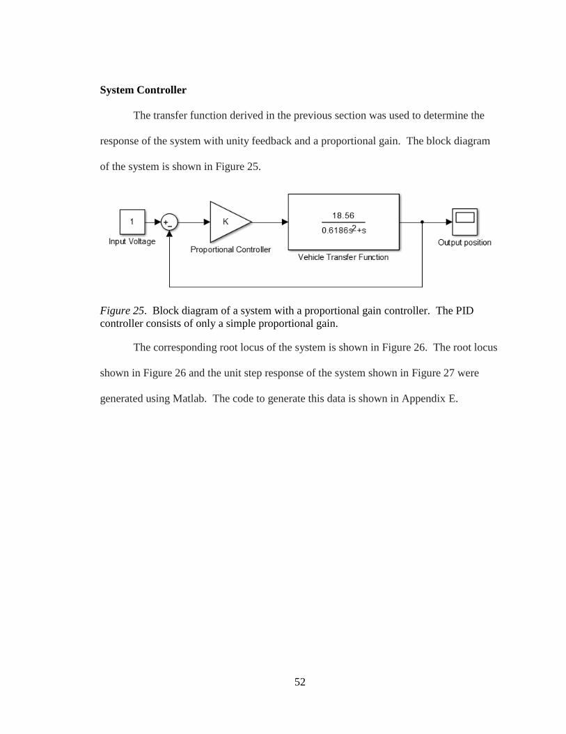
52
System Controller
The transfer function derived in the previous section was used to determine the
response of the system with unity feedback and a proportional gain. The block diagram
of the system is shown in Figure 25.
Figure 25. Block diagram of a system with a proportional gain controller. The PID
controller consists of only a simple proportional gain.
The corresponding root locus of the system is shown in Figure 26. The root locus
shown in Figure 26 and the unit step response of the system shown in Figure 27 were
generated using Matlab. The code to generate this data is shown in Appendix E.

53
Figure 26. Root locus of the open loop transfer function. The fastest response time of
the closed loop system with a proportional gain has a proportional gain equal to 0.0218.
The system open loop transfer function is simply the vehicle transfer function
since there is only a proportional controller. Based on the root locus, the rise time that
can be achieved is 4.15 seconds at a gain of 0.0218 if there is no overshoot. This is
determined by finding the maximum gain where the poles are still on the real axis.
Overshoot is not desired because in a real life system it would be undesirable to
overshoot the platform when pulling into a station. The system response at a gain of
0.0218 is shown in Figure 27.
Root Locus
Real Axis (seconds-1)
Imagin
ary
Axis
(seconds-1
)
-1.8 -1.6 -1.4 -1.2 -1 -0.8 -0.6 -0.4 -0.2 0 0.2-0.5
-0.4
-0.3
-0.2
-0.1
0
0.1
0.2
0.3
0.4
0.5
System: sys1
Gain: 0.0218
Pole: -0.808 - 8.42e-06i
Damping: 1
Overshoot (%): 0
Frequency (rad/s): 0.808

54
Figure 27. Step response of the vehicle with a proportional gain controller. The step
response of the best possible rise time with no overshoot has a gain equal to 0.0218.
Position controller. It was desired that the steady state error in the system be
driven to zero. This is the case with position control since there is an integrator in the
denominator of the plant transfer function. This is shown in equation 46. However, it
was still desirable to achieve improved response times with the system while adjusting
the integral control to overcome friction in the system. Therefore, a proportional integral
derivative (PID) controller was developed to improve the response times. The block
diagram of the controller and overall system is shown in Figure 28.

55
Figure 28. Block diagram of the system with a PID controller. The PID controller was
implemented to improve rise time and minimize steady state error.
To initially tune the parameters in the controller the Ziegler-Nichols (1993)
method was used. In this method, the integral and derivative terms in the controller are
initially set to zero. Then the proportional gain (Kp) is incrementally increased until the
system undergoes sustained oscillations when a step response is input into the system.
Sustained oscillations occur when the proportional gain is set too high and the system
response does not decay to a steady state value.
The system response to a step voltage input was measured by loading the
proportional gain on the microcontroller, setting the vehicle up to wirelessly transmit
position and time values to the master controller, and then applying the step voltage
change to the vehicle. The proportional gain was increased on the vehicle control system
incrementally until is underwent sustained oscillations. The recorded response is shown
in Figure 29 for an ultimate proportional gain (Ku) of 3.
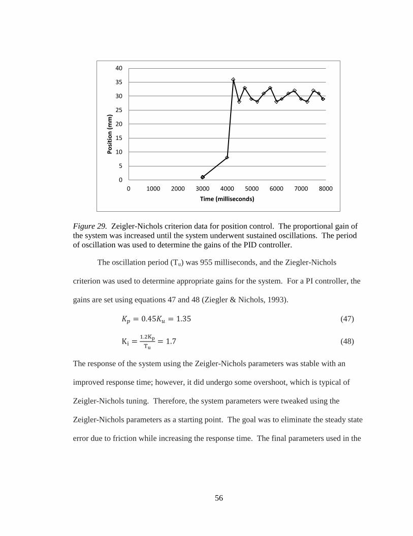
56
Figure 29. Zeigler-Nichols criterion data for position control. The proportional gain of
the system was increased until the system underwent sustained oscillations. The period
of oscillation was used to determine the gains of the PID controller.
The oscillation period (Tu) was 955 milliseconds, and the Ziegler-Nichols
criterion was used to determine appropriate gains for the system. For a PI controller, the
gains are set using equations 47 and 48 (Ziegler & Nichols, 1993).
(47)
(48)
The response of the system using the Zeigler-Nichols parameters was stable with an
improved response time; however, it did undergo some overshoot, which is typical of
Zeigler-Nichols tuning. Therefore, the system parameters were tweaked using the
Zeigler-Nichols parameters as a starting point. The goal was to eliminate the steady state
error due to friction while increasing the response time. The final parameters used in the
0
5
10
15
20
25
30
35
40
0 1000 2000 3000 4000 5000 6000 7000 8000
Po
siti
on
(m
m)
Time (milliseconds)

57
system were Kp=1.5 and Ki=0.03. The system response with these parameters is shown
in Figure 30.
Figure 30. Position with PID controller. The vehicle position is compared to the
position set point.
Figure 30 shows a move from zero to 300 mm with a constantly ramping set
point. The response time of the system is 2.91 seconds. The position follows the set
point well, but at the end of the move the position falls away from the set point. This is
because of increased friction that occurred when the vehicle entered a corner. However,
the integral term increased and moved the vehicle to the appropriate set point
eliminating the steady state error.
Cascaded position velocity controller. The next step in the system was to
develop a velocity controller to control the speed of the vehicle while it is travelling
around the track. This is necessary to allow greater position control and to help ensure
velocity stability when there is a position error. In Figure 31, the velocity of the vehicle
-50
0
50
100
150
200
250
300
350
0 2000 4000 6000 8000
Po
sito
n (
mm
)
Time (milliseconds)
Position
Set Point

58
was measured when a constant input voltage was applied to the dc motor controlling the
vehicle.
Figure 31. Velocity with a step voltage input. The graph shows the velocity of the
vehicle as it travels around the track once.
Figure 31 shows that the velocity of the vehicle is highly dependent on the
position of the vehicle on the track. The dips in velocity occur as the vehicle enters
corners on the track where there is a higher friction. A cascaded position velocity
controller is needed to allow the vehicle to travel at a constant speed when it is travelling
around the track. A cascaded position velocity controller does this by forcing the
position and the velocity to converge to predefined set points for position and velocity,
respectively. Without the cascaded controller, the position controller would force the
position to converge to the set point without regard for the velocity of the vehicle. The
block diagram of the system setup is shown in Figure 32.
0
20
40
60
80
100
120
0 1000 2000 3000 4000 5000 6000 7000
Ve
loci
ty (
mm
/s)
Location (mm)

59
Figure 32. Block diagram of cascaded controller. The cascaded controller consists of an
inside velocity control loop and an outside control loop. A velocity feed-forward loop is
also implemented to improve the velocity response time.
An additional feature that was added in the controller was a velocity feed-forward
loop. This loop approximates what the voltage input should be to the system based on
the velocity set point. This value is then fed forward into the summation calculating the
velocity error. This allows the system to anticipate how it needs to react based on
upcoming circumstances. The values that were needed were approximated by measuring
steady state speed at voltage set points throughout the velocity range of the vehicle.
The velocity of the cascaded controller was tuned by increasing the value of the
proportional gain until the velocity started to oscillate. The gain that it started to oscillate
was 0.8 and the system oscillated with a period of 0.4 seconds. This system response at
this gain is shown in Figure 33.
Position
Controller
∫
Position
Set Point
+ -
Velocity
Controller
Vehicle
Plant
Vehicle
Velocity
+ +
-
Velocity
Set Point
+
+
Disturbance Velocity Feed-forward

60
Figure 33. Zeigler-Nichols criterion data for velocity control. The velocity proportional
gain of the system was increased until the system underwent sustained oscillations. The
period of oscillation was used to determine the gains of the PID controller.
The Zeigler-Nichols criterion was then used to determine initial values to be used
for the gains. The equations to determine the gains are shown in equations 49 through 51
(Ziegler & Nichols, 1993).
(49)
(50)
(51)
These values were used initially with the cascaded controller, but there was still a
significant amount of overshoot with velocity as it hunted for the correct speed. The
gains were tuned to decrease the overshoot and smooth the response. The optimal
coefficients for the real world prototype were Kp=0.3, Ki=0.01, and Kd=0. Additionally,
the position controller coefficients were adjusted to Kp=1.592, Ki=0.01, and Kd=0. These
0
10
20
30
40
50
60
70
80
90
100
0 1000 2000 3000 4000 5000 6000 7000
Ve
loci
ty (
mm
/s)
Time (milliseconds)

61
results were determined by looking at the root locus of the closed loop system and testing
the results on the prototype vehicle.
The first step in determining the optimum coefficients from the root locus was to
minimize the integral gain while ensuring acceptable rise time for the system. This
allowed the system to have low steady state error with a good rise time. The next step
was to increase the derivative gains to improve rise time and setting time. However, after
implementing the derivative control in the system, the derivative control increased the
noise in the system and it sacrificed system robustness. Therefore, the derivative term
was eliminated from the controller. The next step was to look at the root locus and adjust
the proportional gains until just before the poles on the root locus diverged from the real
axis.
The resulting transfer function of the position controller is shown in equation 52
where E is error. The output of the transfer function is a new velocity set point.
( )
( )
(52)
The transfer function for the velocity controller is shown in equation 53.
( )
( )
(53)
The resulting system transfer function is shown in equation 54.
( )
( )
(54)
The root locus, pole zero map, and step response of the system were generated using
Matlab and the code is shown in Appendix F. The root locus is shown in Figure 34.

62
Figure 34. Root locus of cascaded controller. The root locus shows the location of the
closed loop poles as the gain of the controller is increased from zero to infinity. The
proportional gains were increased until just before the poles diverged from the real axis.
The root locus plot shows that there are two poles and two zeros very near the real
axis. This was intentional because the pole placement near the real axis allows the steady
state error to go to zero. The pole was placed near the real axis for both the velocity and
position feedback loops. However, any pole near the real axis slows the response of the
system. In order to counteract this effect, a zero was placed near each pole to cancel out
the slowing effect of the pole. These results are shown in the closed loop pole and zero
map in Figure 35.
-12 -10 -8 -6 -4 -2 0 2-3
-2
-1
0
1
2
3
Root Locus
Real Axis (seconds-1)
Imagin
ary
Axis
(seconds
-1)

63
Figure 35. Closed loop pole and zero map of the cascaded controller. The poles of the
system are indicated by crosses and the poles are indicated by circles.
The pole and zero map shows that there are poles near the real axis to eliminate
steady state error, and there is a zero near each pole to cancel the slowing effect of the
poles near the real axis. Additionally, the two other poles in the system were driven as
far to the left as possible on the real axis by adjusting the gains of the controller. If the
overall gain was adjusted any higher, the poles would leave the real axis, which would
cause undesirable overshoot in the system. The theoretical step response of the closed
loop system based on the model in equation 54 was created in Matlab. The response is
shown in Figure 36. It shows that the response of the system is critically damped which
gives optimum rise time with no overshoot.
-6 -5 -4 -3 -2 -1 0-1
-0.8
-0.6
-0.4
-0.2
0
0.2
0.4
0.6
0.8
1
Pole-Zero Map
Real Axis (seconds-1)
Imagin
ary
Axis
(seconds
-1)

64
Figure 36. Theoretical step response of the cascaded controller. The graph shows the
theoretical step response to a one volt input.
The vehicle position as it travels around the track is shown in Figure 37.
Figure 37. Position with cascaded position velocity controller. The graph shows the
comparison of position set point verses actual position though one lap around the track.
The velocity of the vehicle as it traveled around the track is shown in Figure 38.
0
1000
2000
3000
4000
5000
6000
7000
8000
0 2000 4000 6000 8000 10000 12000 14000
Po
siti
on
(m
m)
Time (milliseconds)
Position Set Point
Position

65
Figure 38. Velocity with cascaded position velocity controller. The graph shows the
comparison of velocity set point verses actual position though one lap around the track.
The previous figures show the position tracks the correct set point within 40 mm.
The velocity also tracks the set point very well; however, the velocity is noisier than the
position data. The velocity resolution can be calculated using equation 55 where v is
actual velocity (mm/s), is estimated velocity (mm/s), R is encoder resolution (mm), and
jT is the time between velocity estimates (ms) (Liu, 2002).
| |
(55)
| |
(56)
| | /s (57)
Equation 57 shows the possible velocity error in the track system. The noise in
the velocity data can be accounted for since the velocity error could be as high as 120
mm/s.
0
100
200
300
400
500
600
700
800
900
0 2000 4000 6000 8000 10000 12000 14000
Ve
loci
ty (
mm
/s)
Time (milliseconds)
Velocity SetPoint
Velocity Car2

66
Additionally, friction is changing constantly as the vehicle travels around the
track. The friction acts as a disturbance to the system and the control system is
constantly reacting to it. The disturbance enters the system as an additional torque that
the motor needs to overcome. This can be described by splitting the vehicle transfer
function into an electrical transfer function and mechanical transfer function and adding
the disturbance torque into the torque needed for the mechanical system. Alternatively,
the disturbance can be converted into a voltage increase needed to produce the additional
torque. The latter approach is shown in the block diagram in Figure 32.
Multiple Vehicle System
The overall system with multiple cars using the cascaded control system was
characterized by putting two vehicles on the track. Both vehicles were programmed to
accelerate to a maximum speed of 700 mm/s and then decelerate to 0 mm/s. The position
set point dictated that the vehicles stop when they completed exactly one lap. The
vehicles’ velocities are shown in Figure 39.

67
Figure 39. Velocity of two moving vehicles. The graph shows a comparison of the
velocity of two moving vehicles that are controlled with position velocity cascaded
controllers.
This figure shows that the velocity of the vehicles is changing relative to each
other but they are both tracking the velocity set point. The positions track the set point
position with 42 mm at all positions around the track and this can be seen in Figure 40.
Figure 40. Position with two vehicles with cascaded controller. The graph shows a
position comparison of two vehicles travelling with a cascaded controller.
0
100
200
300
400
500
600
700
800
900
0 2000 4000 6000 8000 10000 12000 14000
Ve
loci
ty (
mm
/s)
Time (milliseconds)
VelocitySet Point
VelocityCar 2
VelocityCar 1
0
1000
2000
3000
4000
5000
6000
7000
8000
0 5000 10000 15000
Po
siti
on
(m
m)
Time (milliseconds)
Position Car 1
Position Car 2

68
The relative vehicle position is also important because the vehicles cannot crash
into one another. The difference between vehicle positions is shown in Figure 41. The
vehicles started 100 mm apart. The data was normalized to 0 mm by subtracting 100 mm
from the difference in position between the vehicles.
Figure 41. Difference in vehicle position. The graph shows the difference in position
between two vehicles as they travel around the track. The data is normalized to 0 mm.
Figure 41 shows that the position difference between the vehicle can vary as
much as plus or minus 33 mm with an average difference of plus or minus 20 mm. This
corresponds to a full-scale difference in position of 0.96 meters. One method to decrease
this error would be to fully characterize the friction on all tracks the vehicle could run on.
The friction is consistent from vehicle to vehicle as it travels in different locations along
the track. This is because the major source of friction is between the vehicle and the
track. This friction data could then be used to feed-forward a voltage increase at the
corresponding track position.
-40
-30
-20
-10
0
10
20
30
40
0 2000 4000 6000 8000 10000 12000 14000
Po
siti
on
dif
fere
nce
(m
m)
Time (milliseconds)

69
Chapter 4 Conclusions and Recommendations for Future Work
The vehicle and track designed met the objective of the study. The design is a
low cost, easily expandable system so that future development work can be done on the
control systems governing ATN.
Special concern was taken in selecting parts that both met the objective of this
study while minimizing cost. It is imperative that the cost of the platform is low so that
track infrastructure as well as vehicle fleet size can be expanded. This allows a variety of
potential ATN concepts to be tested in real time. The vehicle was designed to be
manufactured with a three-dimensional printer. This was a low-cost solution because of
the availability of the printer. However, the vehicle design could easily be altered so that
it can be manufactured on a milling machine. Alternatively, the design could be adjusted
so that the parts could be cheaply molded if volume requirements are high enough.
Either of these options could be an area for future work if three-dimensional printing is
not an option for manufacturing.
It is also recommended that in future work a printed circuit board assembly
(PCBA) is designed and manufactured for this vehicle. A printed circuit board would
save size, cost, and improve robustness. The microcontroller, XBEE shield, and motor
driver could all be incorporated into a single PCBA. The components of the PCBA
would be significantly less than the cost of buying each component individually. It is
estimated that the cost could be reduced by approximately $50 by implementing a PCBA.
Overall the track assembly was low cost, easy to assemble, and easy to
manufacture. Its performance could be improved by ensuring that each track section is

70
supported at least every 400 mm. After assembling the track, it was determined that the
track is flexible if it is supported less than 400 mm. Alternatively, the thickness of the
sheet metal could be increased to increase its stiffness. However, the material and
manufacturing cost would need to be taken into account before increasing the thickness.
The cascaded control scheme used in this implementation balances the need for
accurate position with maintaining velocity control. This could be improved by
improving the resolution of the velocity estimation. One way to do this would be to
increase the resolution of the linear encoder. Additionally, the control system could be
improved by reducing the friction between the track and the vehicle. A simple upgrade to
decrease friction would be to include a roller in the switching mechanism.
The design of the cascaded controller allows a master controller to be
implemented right on top of the cascaded controller. In fact, the system was designed so
that future work on the master controller would be easy to implement. This architecture
allows the ability to test many master control systems while not having to design the
individual control system for each vehicle.
In future work, the master controller could be updated to include a controller
based on vehicle separation. The current master controller uses set points to tell vehicles
where to go in the system. However, there is no feedback system preventing accidents if
the master controller makes an error or a vehicle breaks down in the guideway.
Therefore, it is recommended that the next steps on this project are to implement a master
controller that takes into account separation distances between vehicles. For example,
the controller would start if the separation distance between vehicles went below a

71
specified threshold. The controller would use the vehicle position to calculate vehicle
separation distance and use this as a feedback mechanism. A master controller such as
this would be more robust and safe because the vehicles would react if a vehicle broke
down in the track guideway to avoid a collision.
Since the beginning of ATN, there has been a substantial amount of theoretical
research and full-scale testing, but there are few scaled physical models that have been
developed to test ATN concepts. The system described here will allow researchers to
further develop control systems and study system operation in order to evaluate and
validate specific questions regarding the implementation of an ATN system. The
modeling approach shown has potential to allow benefits of ATN to be realized and
concerns to be addressed allowing the world to come closer to an environmentally
responsible, economical solution to transportation that passengers will appreciate.

72
References
2getthere. (2012, July). Masdar PRT Application. Retrieved October 24, 2013, from
Sustainable Mobility Solutions: http://www.2getthere.eu/?page_id=10
Aerospace Corporation. (2012). Automated Transit Network Feasibility Evaluation San
José Mineta International Airport San José, CA. El Segundo: Aerospace
Corporation.
Aerospace Corporation. (2014). Aerospace. Retrieved April 26, 2014, from
https://www.aerospace.org/
Anderson, J. (1984). Optimization of Transit-System Characteristics. Journal of
Advanced Transportation, 18(1), 77-111.
Anderson, J. (2000). A Review of the State of the Art of Personal Rapid Transit. Journal
of Advanced Transportation, 34(1), 3-29.
Anderson, J. (2005). The future of high-capacity personal rapid transit. Presentation at
the Advanced Automated Transit Systems Conference. Bologna, Italy.
Austin, M. B. (2001). Building a case for a new transportation system. Retrieved from
http://escholarship.org/uc/item/3fn7j6d2
Carnegie, J., & Voorhees, A. (2007). Viability of Personal Rapid Transit in New Jersey.
New Jersey Department of Transportation.
Digi. (2014, March 10). XBee RF Modules. Retrieved March 27, 2014, from Digi:
http://www.digi.com/products/wireless-wired-embedded-solutions/zigbee-rf-
modules/zigbee-mesh-module/
Fairchield Semiconductor. (2009, September). QRE1113 − Reflective Object Sensor.
Retrieved October 20, 2013, from Fairchild: www.fairchildsemi.com
Helmer, J. R. (2009, March 27). Airport Area Automated Transit Network. San Jose,
California: Santa Clara Transportation Authority.
Irving, J. H. (1978). Fundamentals of Personal Rapid Transit. Lexington, MA: D.C.
Heath and Company.
Kimberly Horn and Associates, Inc. (2010). Assessment of New Tecchnologies: Personal
Rapid Transit. Fresno: Fresno Council of Governments.

73
Krueger, A. (2014, March 28). Automated Transit Network (ATN) prototype [Video file].
Retrieved March 28, 2014, from YouTube: http://youtu.be/K-feorJYHNI
Liu, G. (2002). On velocity Estimation Using Position Measurements. American Control
Conference, (pp. 1115-1120). Anchorage, AK.
Lowson, M. V. (2011). Sustainable Personal Transportation. Forum on Integrated and
Sustainable Transportation Systems (pp. 261-267). Vienna, Austria: IEEE.
Magnovate Technologies. (2013). Magnovate Technologies Realizing the Promise of
Future Transportation Systems. Edmonton, Alberta, Canada.
McDonald, S. S. (2013). Personal Rapid Transit and Its Development. Transportation
Technologies for Sustainability, 831-850.
Movellan, J. (2013, October 15). DC Motors. Retrieved March 20, 2014, from Machine
Perception Laboratory: http://mplab.ucsd.edu/tutorials/DC.pdf
Muller, P. J. (2010). PRT Vendor Updates. PRT News and Views.
Pemberton, M. (2013). The Track to Suncheon: Making APMs Intelligent. Automated
People Movers and Transit Systems, 236-275.
Schneider, J. (2012, September 20). Cabintaxi PRT System. Retrieved January 20, 2014,
from Innovative Transportation Technologies:
https://faculty.washington.edu/jbs/itrans/cabin.htm
Sproule, William J., & Edward S. Neumann. (1991). The Morgantown PRT: It Is Still
Running at West Virginia University. Journal of Advanced Transportation, 269-
279.
Taxi 2000. (2010). Skyweb Express transportation for the 21st Century. Retrieved
October 1, 2013, from
http://faculty.washington.edu/jbs/itrans/SWE%20marketing%20intro.pdf
Taxi 2000. (2013). Skyweb Express. Retrieved November 1, 2013, from Skyweb Express
Technology: http://www.taxi2000.com/technology.html
The Engineering ToolBox. (2014, March 27). Drag Coefficient. Retrieved March 29,
2014, from The Engineering ToolBox: http://www.engineeringtoolbox.com/drag-
coefficient-d_627.html

74
Transport Innovators. (2013, August 1). Why no decent scale models of PRT using off the
shelf robots? (Izmir Institute of Technology PRT Demostration project). Retrieved
August 30, 2013, from Transport Innovators Forum:
https://groups.google.com/forum/#!topic/transport-
innovators/ikdYsIDWCTc%5B1-25-false%5D
Ultra Global. (2013, November 28). ultra pods. Retrieved November 20, 2013, from
Ultra Global PRT: http://www.ultraglobalprt.com/how-it-works/ultra-vehicle/
United States. (1964). Urban Mass Transportation Act of 1964, Pub. L. No. 88-365 § 78,
100 Stat. 302.
Vectus. (2013). Vectus Intelligent Transport. Retrieved November 10, 2013, from
Vectus: http://www.vectus.com
Vectus Ltd. (2012). Media Gallery. Retrieved November 20, 2013, from Vectus
Intelligent Transport: http://www.vectusprt.com/EN/media/images/
Ziegler, & Nichols. (1993). Optimum Settings for Automatic Controllers. Journal of
Dynamic Systems, Measurement, and Control, 759-768.

75
Appendix A
System Design Requirements
1. General
Develop a low-cost, easily portable, simplified, small scale Automated Transportation
Network (ATN) to be used for the demonstration of some of the basic concepts of ATN
transportation systems. This project will also be used for transportation network and
vehicle control development. The ATN shall demonstrate the following:
a. Origin to destination service such that simulated trip requests at a station will
initiate a vehicle traveling from the trip request station to the selected destination
station. If a vehicle is not present at the origin station, an 'empty' vehicle will be
sent to that station.
b. Non-stop vehicle service. Vehicles will not stop at intermediate stations between
the origin station and a destination station.
c. Offline stations allowing vehicles to pass as passengers embark and disembark.
The ATN will not have offline parking of vehicles. However, the system will be
designed to allow for this in a future expansion if desired.
d. Data will be collected on trip requests per unit time (minute), time between trip
request and vehicle departure, and time between vehicle departure and vehicle
arrival. The goal will be to minimize the time between trip requests and vehicle
departure.
e. System capacity by continually adding vehicles until performance starts to
degrade, i.e. vehicle movements begin to interfere with each other.

76
f. Comparison of results to theoretical models and simulations.
2. ATN Controller
The ATN will have a master controller that will do the following:
a. Control routing and movements of all vehicles.
b. Maintain location information on all vehicles.
c. Display vehicle location information in a graphical user interface display. This
will include a layout of the system and location of the vehicles in it.
d. Allow users to set up and design different scenarios of trip generation, including
symmetrical, asymmetrical, random, and manual trip requests.
e. Display number of passengers at stations who have requested vehicles.
f. Allow capability to alter the headway criteria used by the ATN to show how this
affects system capacity as well as safety concerns in case of rapid deceleration.
g. Display a layout of the demonstration track and all conflict points such as
diverges, merges, and station stops.
h. Allow operators to ‘initialize’ vehicles as they are introduced onto the track such
that it enters the location of new vehicles into its inventory.
3. Stations
The stations will have the following characteristics:
a. The stations will be offline with diverges and merges to allow vehicles to exit and
enter the mainline. Vehicles stopped in stations will not impede mainline traffic
flow when they stop to allow passengers to embark and disembark the vehicle.

77
b. Stations will have adequate length ramps to allow vehicles to stop at berthing
position(s).
c. Stations will have adequate length ramps to allow vehicles to accelerate to merge
with mainline traffic.
d. Vehicles will not be able to leave the track at any point through the stations.
e. The stations will have visual displays to indicate the passenger queue count.
f. The stations will have a physical means to allow users to generate a trip request
from that station to any one of the other stations.
4. Vehicles
a. Vehicles will be autonomous with an onboard controller such that they will be
capable of making the trip without input from an outside controller, i.e. store track
layout and routing information.
b. Vehicles will maintain onboard current location in relation to the overall track.
c. Vehicles will have the capability to periodically read a track mounted landmark
and update its current position information accordingly.
d. Vehicles will follow a preset track guide way from one destination to another.
e. Vehicles will maintain a following distance from a vehicle in front to avoid
vehicle collisions.
f. Vehicles will maintain a preset velocity.
g. Vehicles will switch tracks as appropriate to reach the final destination.
h. Vehicles will display total passengers occupying the vehicle.

78
i. Vehicles will be battery powered and maintain a charge for at least five minutes
of continuous use.
5. Track Layout
a. The track will be an oval shape with at least four offline stations.
b. The track will not exceed an 8ft x 8ft footprint and be constructed so as to be
easily assembled and disassembled.
c. The track will not have in track switching.
d. The track will provide guidance for the vehicles so that vehicles will easily stay
within the track.
e. The track will have a vehicle initialization area where vehicles will be introduced
into the ATN.
6. Communications Network
The communications network will provide communications between the vehicles and
ATN controller.
a. The communications network will be robust enough to communicate with at least
10 vehicles.
b. The communication network will reliably transfer route requests to vehicles.
c. The communication network will allow the vehicles to send location information
to the ATN controller and be used by the ATN to communicate the location of
conflict or stopping locations to each vehicle.
d. The communication network will relay quantity of passenger information to the
vehicle.

79
e. The communication network will relay passenger queue information to each
station.
7. Overall hardware and software design requirements
a. The vehicles and track they run on are to be designed from scratch using
commercial off-the-shelf hardware components as well as custom manufactured
pieces. Custom pieces will be manufactured using a three-dimensional printer.
b. The ATN controller will be a commercially available computer.
c. The onboard vehicle controller will be a commercially available microcontroller
for robotic applications.
d. The software language will be C for the onboard vehicle controllers.
8. System Implementation
Due to the large nature of this project, the system will be implemented in stages
with subgroups each tackling specific tasks. There will be meetings as necessary to
coordinate the activities of each sub-group. All work and designs will be documented
and be reviewed within the group at a minimum. The design documentation will provide
information on design philosophies as well as detailed information, i.e. why certain
design approaches were taken, what those approaches were, and how they were
implemented.
Phase 1: A test track and three vehicles will be developed for feasibility testing
of the system. This will include development of both computer aided drafting (CAD)
files and a working prototype that can be tested. The prototype will contain adequate
sensors to control the vehicle by specific position, velocity, and acceleration profiles.

80
Additionally, the prototype will have the ability to maintain specific headways.
Preliminary results will be adequately documented to show the performance of the
system and the ability to expand.
Phase 2: A master controller will be fully developed to perform coordinated
movements of the vehicles which conform to an overall master system approach. The
master controller will have functionality to control the system with multiple simulated
passenger demand scenarios, including symmetric, asymmetric, and random. The system
will have a meaningful graphical user interface that shows the operation of the system
and has data export capability for further analysis. The communication protocol will be
improved so that the system can be expanded until system degrades. Communication
protocol should not be the weakest link. The test track will be improved to contain a
visual display that shows the number of people waiting in the queue at each station.
Phase 3: Expand the project to test system degradation. Maximum capacity is
determined by the maximum number of vehicles that can operate on the system without
interfering with each other, vehicle transit times, and passenger wait times. Multiple
control algorithms should be designed and implemented at this phase to show how the
system reacts under different control algorithms in different loading scenarios.
Additionally, mixed mode operation with different size vehicles can be used to show the
effect of mixed mode operation.

81
Appendix B
Bill of Materials of the Track Assembly
Item
Number Description Quantity
Unit
Cost
Total
Cost
Source
(Part Number)
1 #8 x 0.5in Zinc-
Plated Screws 64
$0.08 $5.12
Lowes
(59177)
2
3/4 x 48 x 96 in
Industrial
Particleboard
2
$20.42 $40.84 Lowes
(12260)
3 Gatehouse 4-in
Door Hinge 3
$0.30 $0.90 Lowes
(308921)
4 Track corner2
out 8
$3.32 $26.56 Solidworks Module
5 Track corner1
in 8
$7.55 $60.40 Solidworks Module
6 Track corner1
out 4
$7.63 $30.52 Solidworks Module
7 Track mirror 4 $8.20 $32.80 Solidworks Module
8 Track straight
long 4
$3.05 $12.20 Solidworks Module
9 Track straight
out 4
$3.00 $12.00 Solidworks Module
10 Tracksplit 4 $8.20 $32.80 Solidworks Module
Total $254.14
Total/foot
of track
$7.70
The cost of custom parts was estimated using the Solidworks Costing Module. The
program has a costing module that will estimate the cost of a custom part based on
machining time and material cost.

82
Appendix C
Bill of Materials for the Vehicle Assembly
Item
Number Description Quantity
Unit
Cost
Total Cost Source
(Part Number)
1 Chassis 1 $20.02 $20.02 Solidworks Module
2 Switch 2 $1.55 $3.10 Solidworks Module
3 Flexure 4 $0.96 $3.84 Solidworks Module
4 Motor Mount 1 $4.50 $4.50 Solidworks Module
5 Wheel 8 $0.50 $4.00 Solidworks Module
6 Shaft 3mm 1 $2.75 $2.75 Mcmaster-Carr
(8920K14)
7 Shaft 1/8 in 1 $1.75 $1.75 Mcmaster-Carr
(8279T16)
8 Worm Gear 1 $2.50 $2.50 Gizmozone
(gw0.5-01014)
9 Worm 1 $2.20 $2.20 Gizmozone
(gwg0.5-26-31)
10 Arduino Uno
R3 1
$29.95 $29.95 Sparkfun
(DEV-11021)
11 XBEE Shield 1 $24.95 $24.95 Sparkfun
(WRL-10854)
12 XBEE Series 2 1 $20.95 $20.95 Sparkfun
(WRL-10414)
13 11.1 V Lithium
Ion Battery 1
$19.55 $19.55 Hobby Partz
(32P-1500mAh-
3S1P-111-20C)
14 QRE1113 Line
Sensor 3
$2.95 $8.85 Sparkfun
(ROB-09454)
15 SN754410
Half-H Driver 1
$2.35 $2.35 Sparkfun
(COM-00315)
16 Scalextric Kit 3 $2.06 $6.18 Scalextric (C8523)
Total $157.44
The cost of custom parts was estimated using the Solidworks Costing Module. The
program has a costing module that will estimate the cost of a custom part based on
machining time and material cost.

83
Appendix D
Drawings of Custom Parts

84
85

86

87
88

89

90

91

92

93

94

95

96

97
Appendix E
Matlab Proportional Controller Code
%% Initialize variables
clc
close all
% Import Data
filename = 'D:\Thesis\Matlab\matlab_system_identification4.txt';
delimiter = '\t';
formatSpec = '%f%f%[^\n\r]';
%% Open the text file.
fileID = fopen(filename,'r');
dataArray = textscan(fileID, formatSpec, 'Delimiter', delimiter, 'ReturnOnError', false);
fclose(fileID);
x = dataArray{:, 1};
x=x/1000;
y = dataArray{:, 2};
%%Import constants
k=0.005;
J=0.0015;
c=.0022 + 9*k^2;
sys=tf(9*k/c,[J/c 1 0]);
%% Proportional Gain
sys1=tf(9*k/c,[J/c 1 0])
[ym,xm]=step(2.7*11.5*sys1);
%step(2.7*11.5*sys1)
xlim([0 10])
figure(1)
rlocus(sys1);
K=0.0218;
H = feedback(K*sys1,1)
figure(2)
step(H)
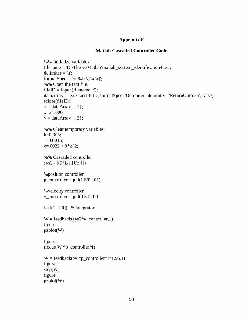
98
Appendix F
Matlab Cascaded Controller Code
%% Initialize variables.
filename = 'D:\Thesis\Matlab\matlab_system_identification4.txt';
delimiter = '\t';
formatSpec = '%f%f%[^\n\r]';
%% Open the text file.
fileID = fopen(filename,'r');
dataArray = textscan(fileID, formatSpec, 'Delimiter', delimiter, 'ReturnOnError', false);
fclose(fileID);
x = dataArray{:, 1};
x=x/1000;
y = dataArray{:, 2};
%% Clear temporary variables
k=0.005;
J=0.0015;
c=.0022 + 9*k^2;
%% Cascaded controller
sys2=tf(9*k/c,[J/c 1])
%position controller
p_controller = pid(1.592,.01)
%velocity controller
v_controller = pid(0.3,0.01)
I=tf(1,[1,0]); %Integrator
W = feedback(sys2*v_controller,1)
figure
pzplot(W)
figure
rlocus(W *p_controller*I)
W = feedback(W *p_controller*I*1.96,1)
figure
step(W)
figure
pzplot(W)

99
Appendix G
Microcontroller Code for the Vehicle
1 #include <XBee.h>
2
3 //Include XBee libraries and set up constants
4 extern volatile unsigned long timer0_millis;
5 //XBee xbee = XBee();
6 //ZBRxResponse ZBRx16 = ZBRxResponse();
7 #define MAX_FRAME_DATA_SIZE 110
8
9 //LED in case of errors
10 #define Err_LED 13
11
12 //QRE1113 variables
13 #define Opto_out A2 //Sensor. High when not on Reflector.
14 #define Opto_in A3 //Sensor. High when not on Reflector.
15 #define Opto_dir A1 //Sensor. High when not on Reflector.
16
17 //Driving Motor Variables
18 #define EN 4
19 #define IN1 5
20 #define IN2 6
21 #define forwardDuty 100
22 #define reverseDuty 30
23 #define FWD 0 //Forward
24 #define REV 1 //Reverse
25
26 //Switch Mechanism Variables
27 #define SWITCH_TIME 800 //900 ms for switch operation
28 #define SWITCH_REST_TIME 2000 // 2000 ms for switch in a position
29 #define SWITCH_RETURN_TIME 2800
30 #define switch_upDuty 50
31
32 //right-hand side motor-controlled switch
33 #define EN_RSwitch 12
34 #define IN1_RSwitch 7
35 #define IN2_RSwitch 11
36 //left-hand side motor-controlled switch
37 #define EN_LSwitch 12
38 #define IN1_LSwitch 3
39 #define IN2_LSwitch 11
40

100
41 //PID variables
42 #define kp 0.3
43 #define ki 0.01
44 #define kv 1.592
45 #define kvd 0
46 #define kvi 0.01
47
48 //time-counter variables
49 long unsigned time_check;
50
51 //DEFINE MORE VARIABLES
52 int o_sensor_in =0;
53 int o_sensor_out=0;
54 int o_sensor_dir=0;
55 long unsigned time_now=0;
56 long unsigned time_last=0;
57 long unsigned time_last_line=0;
58 long unsigned time_line=0;
59 long unsigned switch_start=0;
60 long unsigned time_dir=0;
61 int change=0;
62 int count_sensor=0;
63 long location=-180;
64 byte checkpoint=0;
65 long velocity=0;
66 long vel=0;
67 long vel2=0;
68 long vel3=0;
69 int proximity =0;
70 int count=1;
71 int count_pos=1;
72 int count_vel = 1;
73 int white =0;
74 int white_dir =0;
75 int spillover =0;
76 boolean rest =0;
77 int pause = 0;
78 int pos_check=0;
79 int stoptime =130*2;
80 boolean switch_finished_left=0;
81 boolean switch_finished_right=0;
82 int pos_error =0;
83 int vel_error=0;
84 int last_pos_location=0;

101
85 int last_vel_location=0;
86 int vel_time = 1;
87 long travel_distance= 2452;
88 long max_vel = 700;
89 int vel_feedforward=max_vel/10;
90 int drive =0;
91 int pos_drive = 0;
92 int vel_drive=0;
93 int integral = 0;
94 int vel_integral = 0;
95 int forward=1;
96 boolean got_time =0;
97 float kd= 0;
98 unsigned long pos_setpt = 0;
99 int vel_setpt = 0;
100 int wait=3000;
101 long accel_time=900;
102 long decel_time=1000;
103 long travel_time=(travel_distance-(accel_time*accel_time*max_vel/6000000) -
(max_vel*decel_time/3000)+(decel_time*decel_time*max_vel/6000000))*3000/
max_vel;
104 int accel = wait + accel_time;
105 int travel = wait + accel_time + travel_time;
106 int decel = wait + accel_time+ travel_time + decel_time;
107 int travel_pos =
(accel_time*accel_time*max_vel/6000000)+(travel_time*max_vel/3000);
108 int stop_pos = travel_distance;
109
110 void setup() {
111 pinMode(EN, OUTPUT);
112 pinMode(IN1, OUTPUT);
113 pinMode(IN2, OUTPUT);
114 digitalWrite(EN, LOW); //Prevents motor from spinning at the setup
115 digitalWrite(IN1, HIGH);
116 digitalWrite(IN2, HIGH);
117 pinMode(Err_LED, OUTPUT);
118 pinMode(EN_RSwitch, OUTPUT);
119 pinMode(IN1_RSwitch, OUTPUT);
120 pinMode(IN2_RSwitch, OUTPUT);
121 pinMode(EN_LSwitch, OUTPUT);
122 pinMode(IN1_LSwitch, OUTPUT);
123 pinMode(IN2_LSwitch, OUTPUT);
124 pinMode(Opto_out, INPUT);
125 pinMode(Opto_in, INPUT);
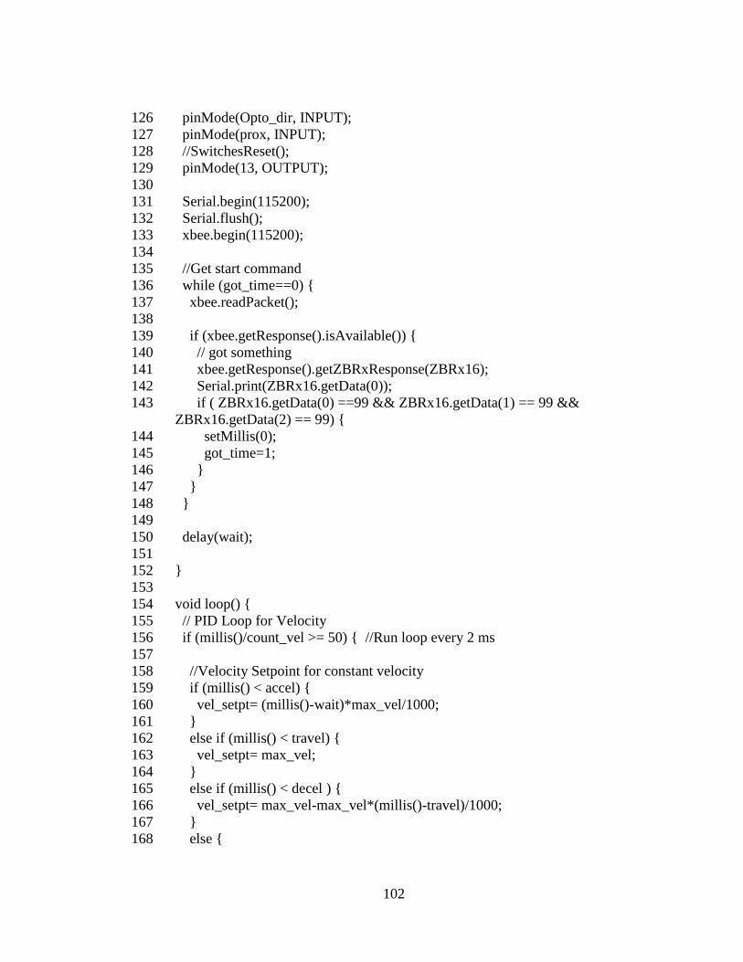
102
126 pinMode(Opto_dir, INPUT);
127 pinMode(prox, INPUT);
128 //SwitchesReset();
129 pinMode(13, OUTPUT);
130
131 Serial.begin(115200);
132 Serial.flush();
133 xbee.begin(115200);
134
135 //Get start command
136 while (got_time==0) {
137 xbee.readPacket();
138
139 if (xbee.getResponse().isAvailable()) {
140 // got something
141 xbee.getResponse().getZBRxResponse(ZBRx16);
142 Serial.print(ZBRx16.getData(0));
143 if ( ZBRx16.getData(0) ==99 && ZBRx16.getData(1) == 99 &&
ZBRx16.getData(2) == 99) {
144 setMillis(0);
145 got_time=1;
146 }
147 }
148 }
149
150 delay(wait);
151
152 }
153
154 void loop() {
155 // PID Loop for Velocity
156 if (millis()/count_vel >= 50) { //Run loop every 2 ms
157
158 //Velocity Setpoint for constant velocity
159 if (millis() < accel) {
160 vel_setpt= (millis()-wait)*max_vel/1000;
161 }
162 else if (millis() < travel) {
163 vel_setpt= max_vel;
164 }
165 else if (millis() < decel ) {
166 vel_setpt= max_vel-max_vel*(millis()-travel)/1000;
167 }
168 else {

103
169 vel_setpt=0;
170 }
171
172
173 if (millis()/vel_time >= 5) { //Update Velocity loop every 5 ms
174 velocity=(location-vel3)*20; //mm/s
175
176 //Update count of velocity
177 vel3=vel2;
178 vel2=last_vel_location;
179 last_vel_location=location;
180 vel_time = vel_time +1;
181 }
182
183 //Find velocity error
184 vel_error=vel_setpt-velocity;
185
186 //Integral for velocity
187 if (abs(vel_error) <= 3) {
188 vel_integral=0;
189 }
190 else if (abs(vel_integral) > 255/kvi) {
191 vel_integral=255/kvi;
192 }
193 //Integral threshold anti-windup
194 else if (abs(vel_error) < 100) {
195 vel_integral=vel_integral + 0.1*vel_error;
196 }
197 else {
198 vel_integral =0;
199 }
200
201 //Controller
202 vel_drive = kv*vel_error + kvi*vel_integral + kvd*(vel3-location);
203
204
205
206 //Update the velocity loop count
207 count_vel = count_vel + 1;
208 }
209
210
211 //*************PID CONTROLLER position****************
212 if ((millis())/count_pos >= 10) { //Run loop every 10 ms

104
213 //Position setpoint for constant velocity
214 if (millis() < accel ) {
215 pos_setpt=((millis()-wait))*((millis()-wait))*max_vel/2000000/3;
216 }
217 else if ( millis() < travel) {
218 pos_setpt=accel_time*accel_time*max_vel/6000000+(millis()-
accel)*max_vel/3000;
219 }
220 else if (millis() < decel) {
221 pos_setpt=travel_pos +(millis()-travel)*max_vel/3000-(millis()-
travel)*(millis()-travel)*max_vel/6000000;
222 }
223 else if (millis() >= decel) {
224 pos_setpt=stop_pos;
225 }
226
227
228 //Position error
229 pos_error= pos_setpt-location;
230 if (abs(pos_error) <= 1) {
231 integral=0;
232 }
233 else if (abs(integral) > 255/ki) {
234 integral=255/ki;
235 }
236 //Integral threshold anti-windup
237 else if (abs(pos_error) < 50) {
238 integral=integral + pos_error;
239 }
240 else {
241 integral =0;
242 }
243
244 //Controller
245 pos_drive = kp*pos_error + ki*integral + kd*(last_pos_location-location);
246 last_pos_location= location;
247 count_pos = count_pos + 1;
248
249 }
250 // vel_feedforward=0;
251 if (millis() < accel) {
252 vel_feedforward=max_vel/11 + 0;
253 }
254 else if ((location) > 180 && (location) < 610) {

105
255 vel_feedforward=max_vel/10 +50;
256 }
257 else if ((location) > 650 && (location) < 700) {
258 vel_feedforward=max_vel/10 -10;
259 }
260 else if ((location) > 800 && (location) < 1150) {
261 vel_feedforward=max_vel/10 +60;
262 }
263 else if ((location) > 1400 && (location) < 1706) {
264 vel_feedforward=max_vel/10 +50;
265 }
266 else if ((location) > 2000 && (location) < 2169) {
267 vel_feedforward=max_vel/10 +50;
268 }
269 else {
270 vel_feedforward=max_vel/10 + 5;
271 }
272
273 //Update the voltage delivered to motor
274 if (abs(stop_pos-location) < 2) {
275 drive =0;
276 }
277 else {
278 drive = pos_drive + vel_drive + vel_feedforward;
279 }
280
281 Motor(drive);
282
283 if (checkpoint==0 || ((checkpoint%10)*100+location) > stoptime ) {
284 //Turn on second sensor
285 o_sensor_in =analogRead(3);
286
287 if( o_sensor_in > 600 && (millis()-pause) >1000) {
288
289 checkpoint=10-checkpoint%10+checkpoint;
290 pos_check=location;
291 //location=0;
292 pause=millis();
293 }
294 }
295
296 if ((millis())/count_sensor >= 1) { //Read optical sensor
297 o_sensor_out =analogRead(2);
298 o_sensor_dir =analogRead(1);

106
299
300
301 if( o_sensor_out > 470 && white ==1) {
302 time_last = time_now;
303 time_now=millis();
304 //Update Velocity
305 vel = 3000/(time_now-time_last); //Velocity: 1000000*mm/us = mm/s
306 white =0;
307
308 //Only use quadrature encoder if the vehicle is moving slow
309 if (vel > 300) {
310 forward =1;
311 }
312 else
313 {
314 //Check time_dir to ensure it is a valid number
315 if (vel ==0) {
316 forward = drive/abs(drive); //if velocity is zero then direction equals drive
direction
317 }
318 else if (time_dir > time_last) { //Don't change direction if time_dir is not valid
319 if ((time_dir-time_last) < (time_now-time_dir)) {
320 forward =1; //Motor is going forward
321 }
322 else if ((time_dir-time_last) > (time_now-time_dir)) {
323 forward=-1;
324 }
325 }
326 }
327
328 //Check if the location is going to roll over
329 if (location==255 && forward ==1){
330 checkpoint=checkpoint +1;
331 }
332 else if (location==0 && forward == -1){
333 checkpoint=checkpoint -1;
334 }
335 //Update location and velocity
336 location=location + forward;
337 }
338 else if (white ==0 && o_sensor_out < 450){
339 time_last = time_now;
340 time_now=millis();
341 //Update Velocity

107
342 vel = 3000/(time_now-time_last); //Velocity: mm/s
343
344 white = 1;
345
346 if (vel > 300) {
347 forward =1;
348 }
349 else {
350 //Check time_dir to ensure it is a valid number
351 if (vel ==0) {
352 forward = drive/abs(drive); //if velocity is 0,direction equals drive direction
353 }
354 else if (time_dir > time_last) { //Don't change direction if time_dir is not valid,
355 if ((time_dir-time_last) < (time_now-time_dir)) {
356 forward =1; //Motor is going forward
357 }
358 else if ((time_dir-time_last) > (time_now-time_dir)) {
359 forward=-1;
360 }
361 }
362 }
363
364 //Check if the location is going to roll over
365 if (location==255 && forward ==1){
366 checkpoint=checkpoint +1;
367 }
368 else if (location==0 && forward == -1){
369 checkpoint=checkpoint -1;
370 }
371 //Update location and velocity
372 location=location + forward;
373 }
374
375 //Quadrature Sensor data
376 if( o_sensor_dir > 230 && white_dir ==1) {
377 time_dir=micros()+0000;
378 white_dir= 0;
379 }
380 else if( o_sensor_dir < 220 && white_dir ==0) {
381 time_dir=micros()+4000; //Constant to shift the waveform
382 white_dir= 1;
383 }
384 }
385 //Stop Commands
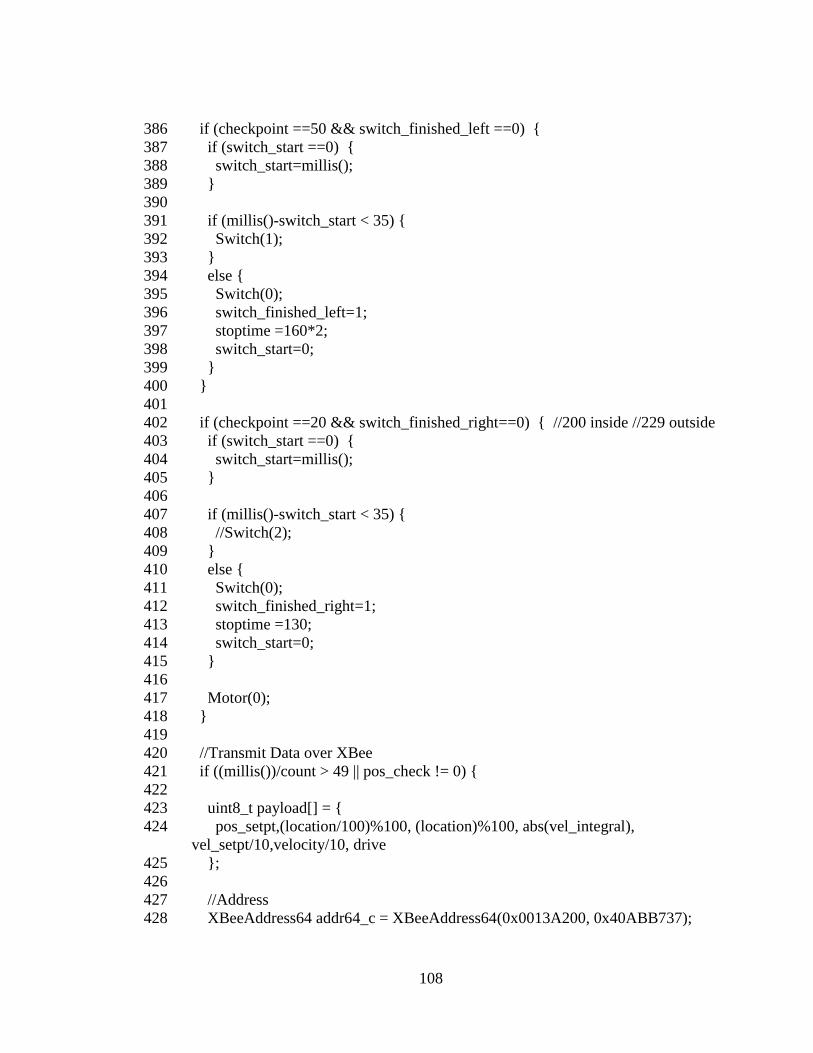
108
386 if (checkpoint ==50 && switch_finished_left ==0) {
387 if (switch_start ==0) {
388 switch_start=millis();
389 }
390
391 if (millis()-switch_start < 35) {
392 Switch(1);
393 }
394 else {
395 Switch(0);
396 switch_finished_left=1;
397 stoptime =160*2;
398 switch_start=0;
399 }
400 }
401
402 if (checkpoint ==20 && switch_finished_right==0) { //200 inside //229 outside
403 if (switch_start ==0) {
404 switch_start=millis();
405 }
406
407 if (millis()-switch_start < 35) {
408 //Switch(2);
409 }
410 else {
411 Switch(0);
412 switch_finished_right=1;
413 stoptime =130;
414 switch_start=0;
415 }
416
417 Motor(0);
418 }
419
420 //Transmit Data over XBee
421 if ((millis())/count > 49 || pos_check != 0) {
422
423 uint8_t payload[] = {
424 pos_setpt,(location/100)%100, (location)%100, abs(vel_integral),
vel_setpt/10,velocity/10, drive
425 };
426
427 //Address
428 XBeeAddress64 addr64_c = XBeeAddress64(0x0013A200, 0x40ABB737);
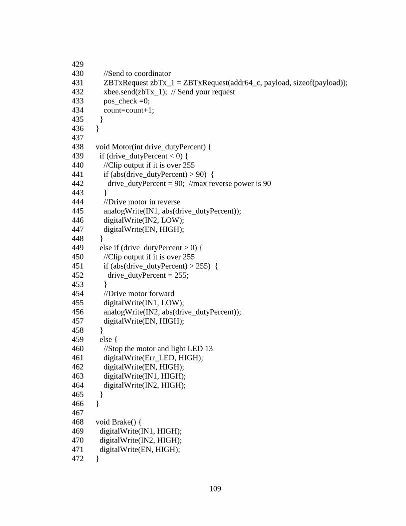
109
429
430 //Send to coordinator
431 ZBTxRequest zbTx_1 = ZBTxRequest(addr64_c, payload, sizeof(payload));
432 xbee.send(zbTx_1); // Send your request
433 pos_check =0;
434 count=count+1;
435 }
436 }
437
438 void Motor(int drive_dutyPercent) {
439 if (drive_dutyPercent < 0) {
440 //Clip output if it is over 255
441 if (abs(drive_dutyPercent) > 90) {
442 drive_dutyPercent = 90; //max reverse power is 90
443 }
444 //Drive motor in reverse
445 analogWrite(IN1, abs(drive_dutyPercent));
446 digitalWrite(IN2, LOW);
447 digitalWrite(EN, HIGH);
448 }
449 else if (drive_dutyPercent > 0) {
450 //Clip output if it is over 255
451 if (abs(drive_dutyPercent) > 255) {
452 drive_dutyPercent = 255;
453 }
454 //Drive motor forward
455 digitalWrite(IN1, LOW);
456 analogWrite(IN2, abs(drive_dutyPercent));
457 digitalWrite(EN, HIGH);
458 }
459 else {
460 //Stop the motor and light LED 13
461 digitalWrite(Err_LED, HIGH);
462 digitalWrite(EN, HIGH);
463 digitalWrite(IN1, HIGH);
464 digitalWrite(IN2, HIGH);
465 }
466 }
467
468 void Brake() {
469 digitalWrite(IN1, HIGH);
470 digitalWrite(IN2, HIGH);
471 digitalWrite(EN, HIGH);
472 }

110
473
474 void Switch(int switch_direction) {
475 if (switch_direction == 1) { // left switch down
476 analogWrite(IN1_RSwitch, 235);
477 digitalWrite(IN2_RSwitch, LOW);
478 digitalWrite(EN_RSwitch, HIGH);
479 }
480 if (switch_direction == 2) { //right switch down
481 analogWrite(IN2_RSwitch, 235);
482 digitalWrite(IN1_RSwitch, LOW);
483 digitalWrite(EN_RSwitch, HIGH);
484 }
485 if (switch_direction == 0) { //Stops the switch
486 digitalWrite(IN1_RSwitch, HIGH);
487 digitalWrite(IN2_RSwitch, HIGH);
488 digitalWrite(EN_RSwitch, HIGH);
489 }
490 }
491
492 void setMillis(unsigned long new_millis){
493 uint8_t oldSREG = SREG;
494 cli();
495 timer0_millis = new_millis;
496 SREG = oldSREG;
497 }